TUTORIAL FOR IMPORTING OTTAWA FIRE HYDRANT

PARKING VIOLATION DATA INTO MYSQL

We have spent the first part of the course learning Excel:

importing files, cleaning, sorting, filtering, pivot tables and

exporting filtered datasets into new files.

Now it’s time to graduate to MySQL, which has the advantage

of being able to work with multiple tables with millions of

records.

We have already successfully downloaded MySQL onto your

computers by either using the tutorial for Windows or Macs, or

MAMP pro for Windows.

Now, we will import the dataset that contains the 2008

violations for parking too close to fire hydrants that formed the

basis of Steve Rennie’s story.

So let’s get started.

1. Download the city of Ottawa’s 2008 by clicking here.

2. Save the file to a folder set up for this exercise.

3. Make a copy and work from the backup.

4. You’ll notice that this is ONLY violations from 2008. We

will be adding subsequent years to this dataset, using

“UNION ALL” query. This 2008 dataset represents a

starting point to creating a master file covering the years

2008 to the first several months of 2014.

5. Make sure that the backup version for this tutorial is on

your C-drive if you have a PC or your desktop if you have a

Mac.

6. Open the file. You’ll notice that the dates in the date

columns are ordered year, month, day. This is the order

the dates must be in. Otherwise, MySQL will import the

dates as zeros.

7. Open MySQL Workbench.

8. We must create a “SCHEMA”.

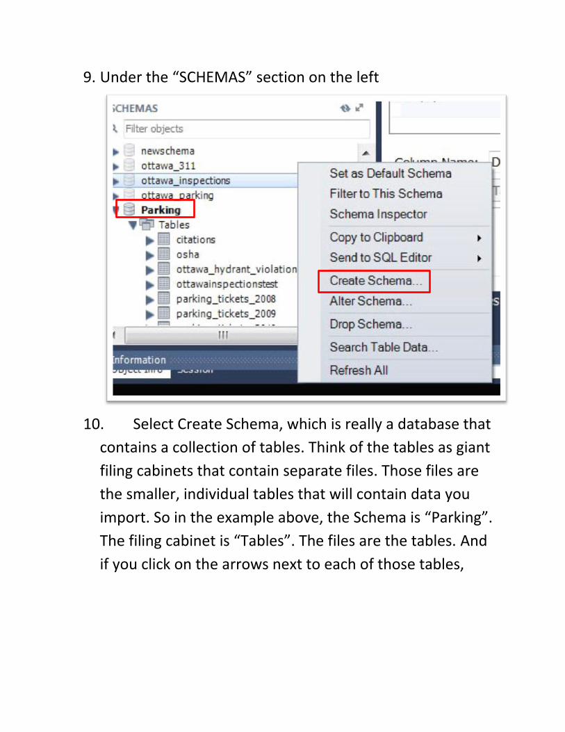
9. Under the “SCHEMAS” section on the left

10. Select Create Schema, which is really a database that

contains a collection of tables. Think of the tables as giant

filing cabinets that contain separate files. Those files are

the smaller, individual tables that will contain data you

import. So in the example above, the Schema is “Parking”.

The filing cabinet is “Tables”. The files are the tables. And

if you click on the arrows next to each of those tables,

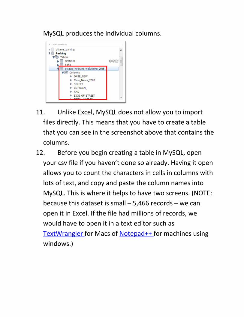
MySQL produces the individual columns.

11. Unlike Excel, MySQL does not allow you to import

files directly. This means that you have to create a table

that you can see in the screenshot above that contains the

columns.

12. Before you begin creating a table in MySQL, open

your csv file if you haven’t done so already. Having it open

allows you to count the characters in cells in columns with

lots of text, and copy and paste the column names into

MySQL. This is where it helps to have two screens. (NOTE:

because this dataset is small – 5,466 records – we can

open it in Excel. If the file had millions of records, we

would have to open it in a text editor such as

TextWrangler for Macs of Notepad++ for machines using

windows.)

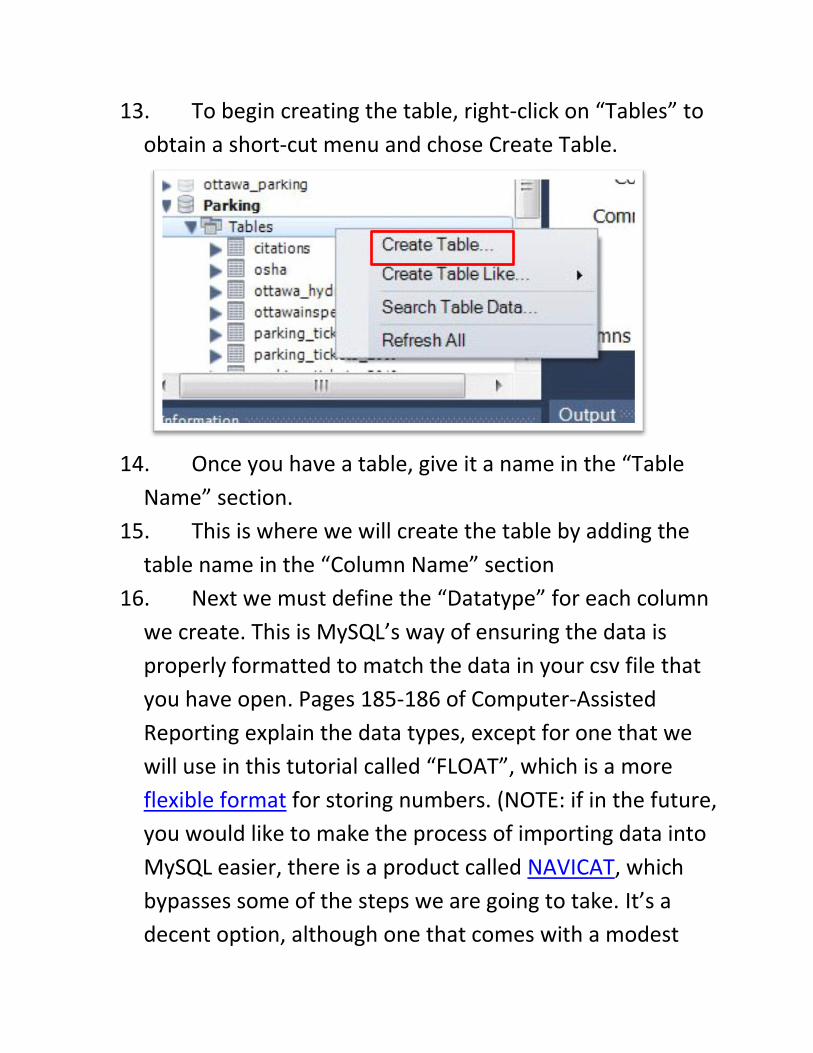
13. To begin creating the table, right-click on “Tables” to

obtain a short-cut menu and chose Create Table.

14. Once you have a table, give it a name in the “Table

Name” section.

15. This is where we will create the table by adding the

table name in the “Column Name” section

16. Next we must define the “Datatype” for each column

we create. This is MySQL’s way of ensuring the data is

properly formatted to match the data in your csv file that

you have open. Pages 185-186 of Computer-Assisted

Reporting explain the data types, except for one that we

will use in this tutorial called “FLOAT”, which is a more

flexible format for storing numbers. (NOTE: if in the future,

you would like to make the process of importing data into

MySQL easier, there is a product called NAVICAT, which

bypasses some of the steps we are going to take. It’s a

decent option, although one that comes with a modest

price tag. However, there is a lot to be said for learning

how to do things manually, which leads to a better

understanding of importing data into MySQL. Such an

improved understanding also makes it easier to

troubleshoot, which is always the frustrating part of

working with data.)

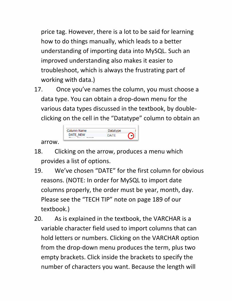
17. Once you’ve names the column, you must choose a

data type. You can obtain a drop-down menu for the

various data types discussed in the textbook, by double-

clicking on the cell in the “Datatype” column to obtain an

arrow.

18. Clicking on the arrow, produces a menu which

provides a list of options.

19. We’ve chosen “DATE” for the first column for obvious

reasons. (NOTE: In order for MySQL to import date

columns properly, the order must be year, month, day.

Please see the “TECH TIP” note on page 189 of our

textbook.)

20. As is explained in the textbook, the VARCHAR is a

variable character field used to import columns that can

hold letters or numbers. Clicking on the VARCHAR option

from the drop-down menu produces the term, plus two

empty brackets. Click inside the brackets to specify the

number of characters you want. Because the length will

vary, you must choose the maximum length. So say the

number of characters varied from 10 to 60. You would

choose a VARCHAR of 60, or 65 just be on the safe side.

This involves counting the number of characters in the

column that contains the greatest numbers, which is easy

because you have the csv file open!! This means doing a

manual count. (NOTE: if the column has long text strings

that make counting tricky, you could automate the process

by creating a new column in Excel and using the LEN

function (“=LEN(cell reference”) which produces the

character length for that cell, You could then copy the

formula, sort in descending order to easily obtain the

maximum and minimum values in the range. Once you

have the range of character lengths, just delete the

column.)

21. For the columns that contain the fine amounts, we

will use the “FLOAT” option, which is a bit more flexible

than double, a format that allows decimal places.

22. And you will also have to add an extra column at the

end that will cut down on the “truncation” errors that

occur. I’ve called that column “Empty”. However, the exact

name doesn’t matter.

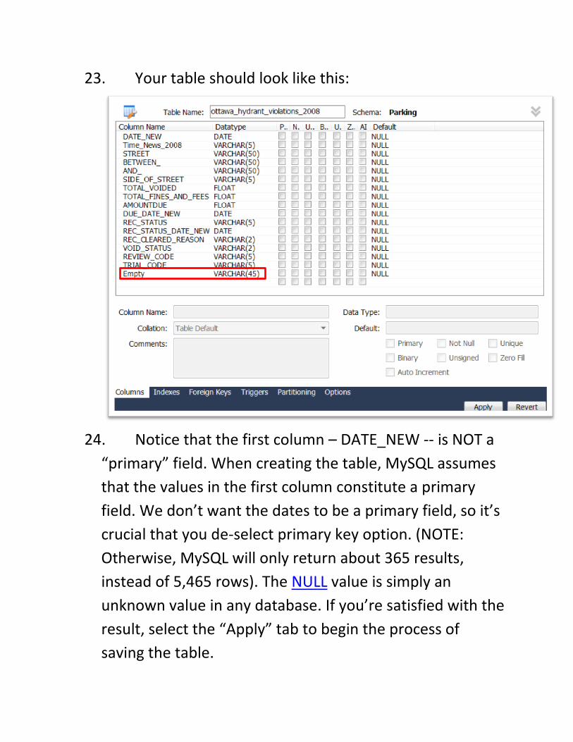
23. Your table should look like this:

24. Notice that the first column – DATE_NEW -- is NOT a

“primary” field. When creating the table, MySQL assumes

that the values in the first column constitute a primary

field. We don’t want the dates to be a primary field, so it’s

crucial that you de-select primary key option. (NOTE:

Otherwise, MySQL will only return about 365 results,

instead of 5,465 rows). The NULL value is simply an

unknown value in any database. If you’re satisfied with the

result, select the “Apply” tab to begin the process of

saving the table.

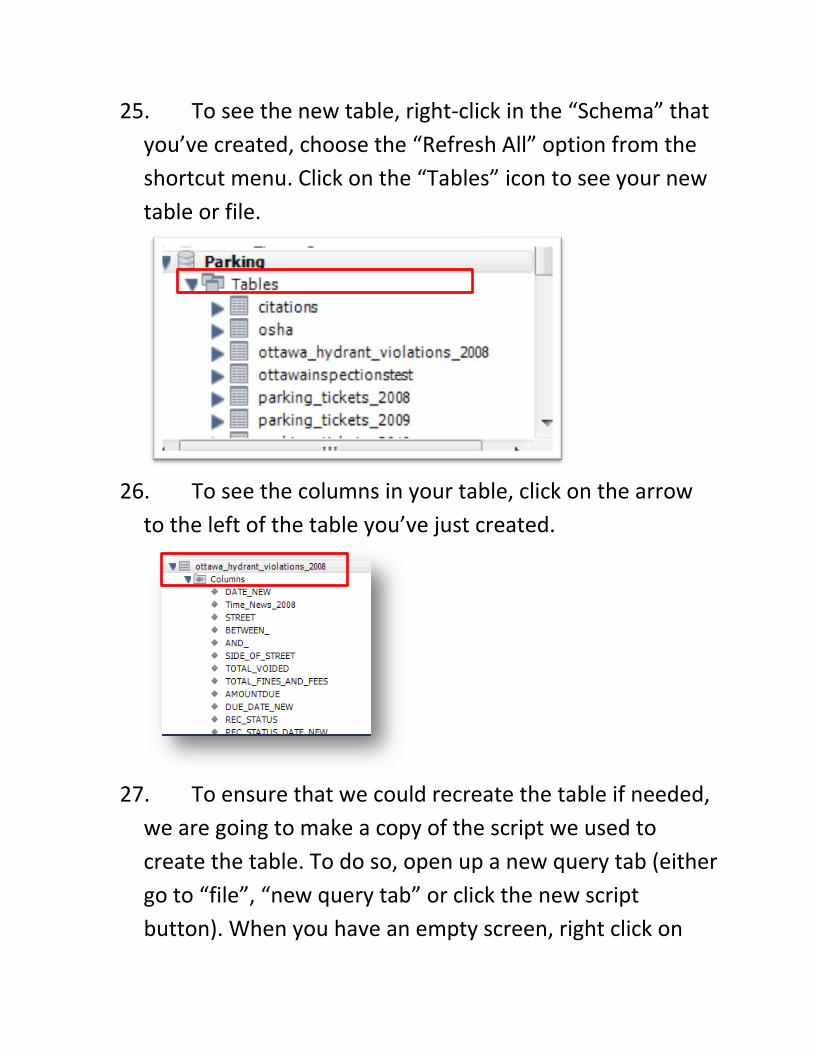
25. To see the new table, right-click in the “Schema” that

you’ve created, choose the “Refresh All” option from the

shortcut menu. Click on the “Tables” icon to see your new

table or file.

26. To see the columns in your table, click on the arrow

to the left of the table you’ve just created.

27. To ensure that we could recreate the table if needed,

we are going to make a copy of the script we used to

create the table. To do so, open up a new query tab (either

go to “file”, “new query tab” or click the new script

button). When you have an empty screen, right click on

the table you created along the left hand side, go down to

“send to SQL editor” and select “Create Statement”. This

will copy the script used to create your table into your

editor. Save this file into a spot you can find, so that we

can use it later for future years.

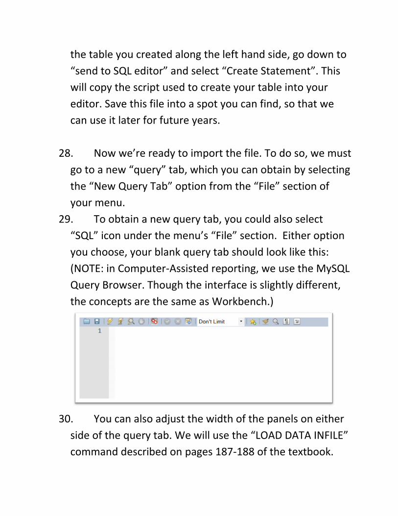
28. Now we’re ready to import the file. To do so, we must

go to a new “query” tab, which you can obtain by selecting

the “New Query Tab” option from the “File” section of

your menu.

29. To obtain a new query tab, you could also select

“SQL” icon under the menu’s “File” section. Either option

you choose, your blank query tab should look like this:

(NOTE: in Computer-Assisted reporting, we use the MySQL

Query Browser. Though the interface is slightly different,

the concepts are the same as Workbench.)

30. You can also adjust the width of the panels on either

side of the query tab. We will use the “LOAD DATA INFILE”

command described on pages 187-188 of the textbook.

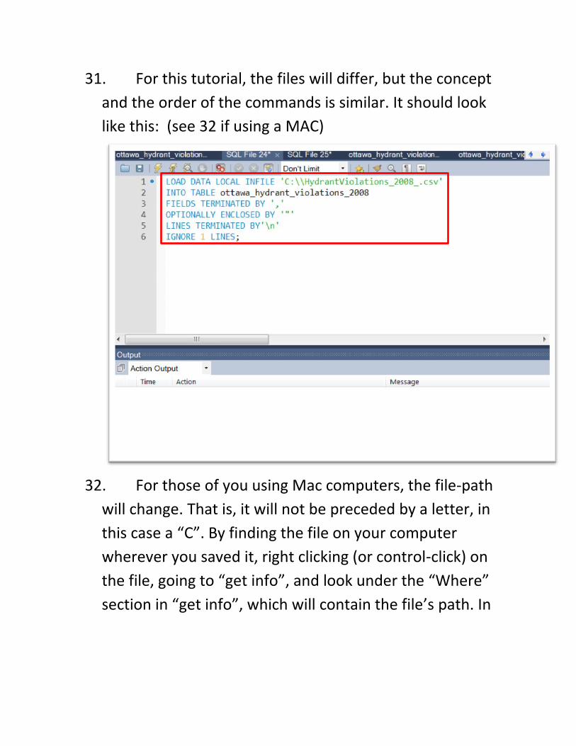
31. For this tutorial, the files will differ, but the concept

and the order of the commands is similar. It should look

like this: (see 32 if using a MAC)

32. For those of you using Mac computers, the file-path

will change. That is, it will not be preceded by a letter, in

this case a “C”. By finding the file on your computer

wherever you saved it, right clicking (or control-click) on

the file, going to “get info”, and look under the “Where”

section in “get info”, which will contain the file’s path. In

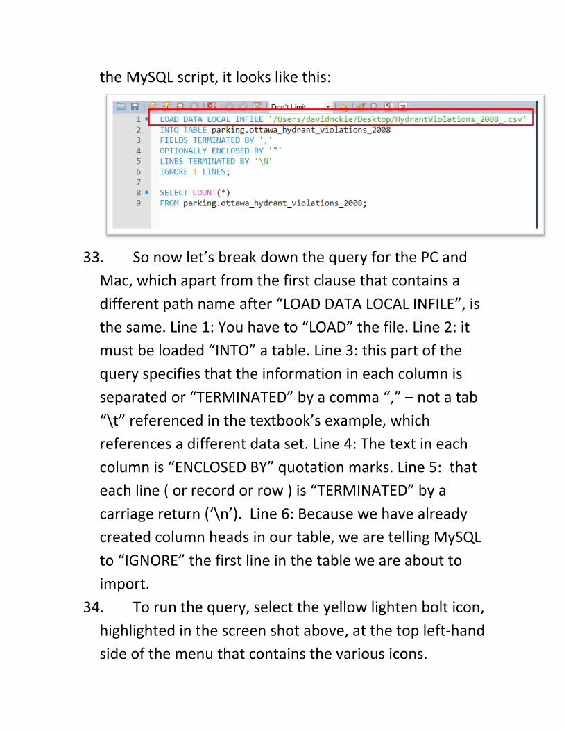
the MySQL script, it looks like this:

33. So now let’s break down the query for the PC and

Mac, which apart from the first clause that contains a

different path name after “LOAD DATA LOCAL INFILE”, is

the same. Line 1: You have to “LOAD” the file. Line 2: it

must be loaded “INTO” a table. Line 3: this part of the

query specifies that the information in each column is

separated or “TERMINATED” by a comma “,” – not a tab

“\t” referenced in the textbook’s example, which

references a different data set. Line 4: The text in each

column is “ENCLOSED BY” quotation marks. Line 5: that

each line ( or record or row ) is “TERMINATED” by a

carriage return (‘\n’). Line 6: Because we have already

created column heads in our table, we are telling MySQL

to “IGNORE” the first line in the table we are about to

import.

34. To run the query, select the yellow lighten bolt icon,

highlighted in the screen shot above, at the top left-hand

side of the menu that contains the various icons.

35. You will get some “truncation” errors. Please ignore

them for now, as they will not affect the data you are

about to import.

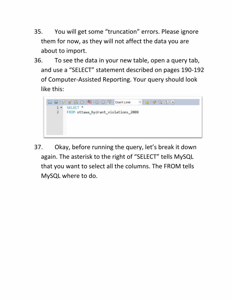
36. To see the data in your new table, open a query tab,

and use a “SELECT” statement described on pages 190-192

of Computer-Assisted Reporting. Your query should look

like this:

37. Okay, before running the query, let’s break it down

again. The asterisk to the right of “SELECT” tells MySQL

that you want to select all the columns. The FROM tells

MySQL where to do.

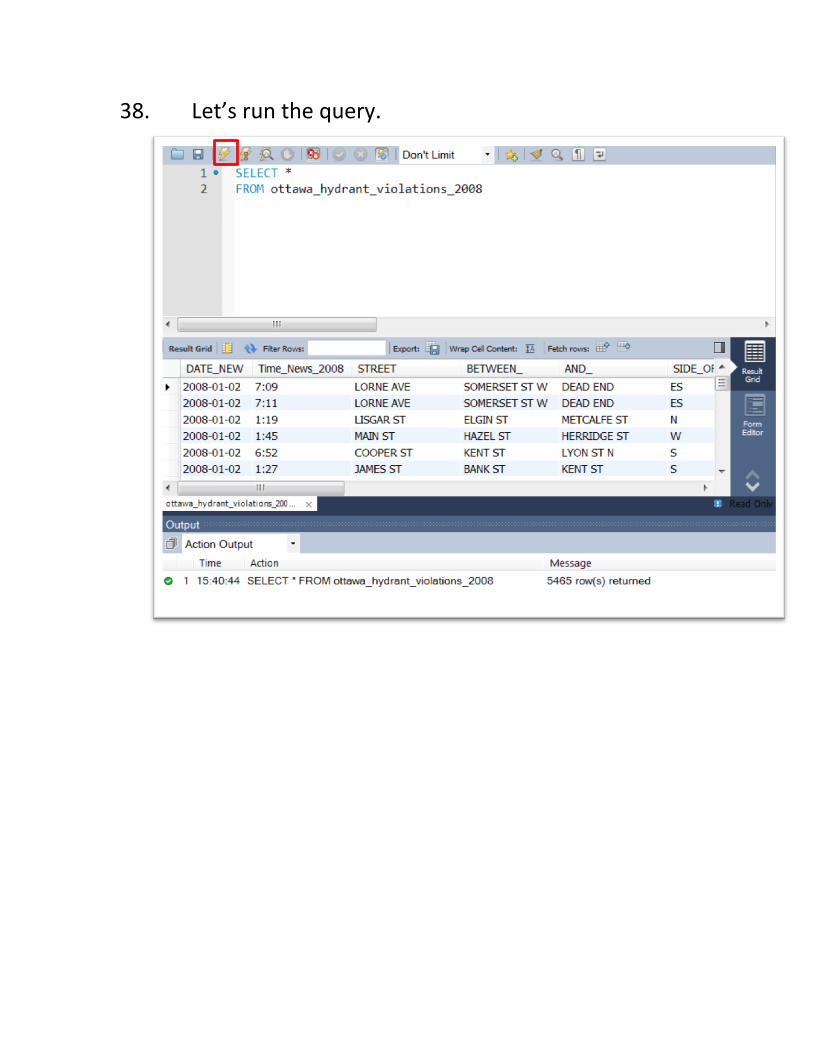
38. Let’s run the query.

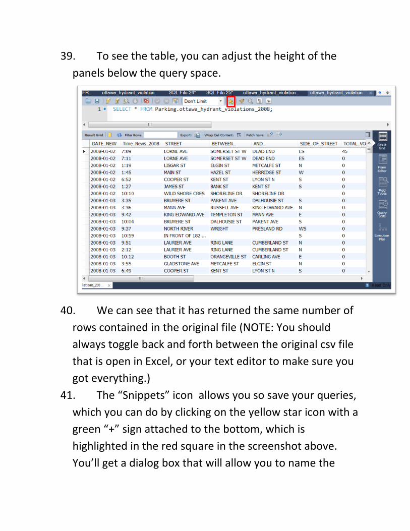
39. To see the table, you can adjust the height of the

panels below the query space.

40. We can see that it has returned the same number of

rows contained in the original file (NOTE: You should

always toggle back and forth between the original csv file

that is open in Excel, or your text editor to make sure you

got everything.)

41. The “Snippets” icon allows you so save your queries,

which you can do by clicking on the yellow star icon with a

green “+” sign attached to the bottom, which is

highlighted in the red square in the screenshot above.

You’ll get a dialog box that will allow you to name the

query, which will then be deposited to the right of the

table. You can also save the query by clicking on the “Save

Script” option in the “File” portion of the menu above. Be

sure to designate the area on your hard drive where you

want to save the script.

42. As one additional final step, you can output the data

in your MYSQL table through a simple query.

SELECT * FROM Ottawa_hydrant_violations_2008 INTO

OUTFILE “filepath.csv” FIELDS TERMINATED BY “,”

ENCLOSED BY “””” LINES TERMINATED BY “/n”;

Ensure that the file-path is ended by “.csv” to create a csv

file.

This will create a new file, which can be manipulated in

Excel or MYSQL, same as the files you’ve been

downloading from the internet.

43. Now that you’ve downloaded a file, you can

experiment with some of the queries described in our

textbook.

44. We will be continuing this exercise in class with

subsequent years. So it’s important that you accomplish

the tasks set out in this tutorial.

45. For more detailed information about MySQL, you can

visit:

http://dev.mysql.com/doc/refman/5.5/en/index.html