tutorial for the nag fortran 90 library · 2019-02-07 · introduction tutorial tutorial for the...
TRANSCRIPT
Introduction Tutorial
Tutorial for the NAG Fortran 90 Library
Contents
0 How to Use this Tutorial 0.2.2
1 Example 1: Displaying Information About the Library 0.2.21.1 Accessing the Library . . . . . . . . . . . . . . . . . . . . . . . . . . . . . . . . . . . . . . . . . . . 0.2.21.2 Finding the Documentation You Need . . . . . . . . . . . . . . . . . . . . . . . . . . . 0.2.21.3 A First Program . . . . . . . . . . . . . . . . . . . . . . . . . . . . . . . . . . . . . . . . . . . . . . . . 0.2.31.4 Remarks on Programming Style and Conventions . . . . . . . . . . . . . . . . 0.2.31.5 USE Statements and Compile-time Errors . . . . . . . . . . . . . . . . . . . . . . . . 0.2.4
2 Example 2: Evaluating a Special Function 0.2.42.1 Arguments of Real Type . . . . . . . . . . . . . . . . . . . . . . . . . . . . . . . . . . . . . . . . 0.2.42.2 Precision and Kind Values . . . . . . . . . . . . . . . . . . . . . . . . . . . . . . . . . . . . . . . 0.2.62.3 Portable Programming for Real Data . . . . . . . . . . . . . . . . . . . . . . . . . . . . 0.2.62.4 Arguments of intent(in) and Passing Constants as Arguments . . . . 0.2.72.5 A First Look at Run-time Errors . . . . . . . . . . . . . . . . . . . . . . . . . . . . . . . . 0.2.8
3 Example 3: Summary Statistics of Univariate Data 0.2.93.1 A First Look at Array Arguments . . . . . . . . . . . . . . . . . . . . . . . . . . . . . . . 0.2.93.2 Passing Array Sections as Arguments . . . . . . . . . . . . . . . . . . . . . . . . . . . . 0.2.103.3 Using Allocatable Arrays . . . . . . . . . . . . . . . . . . . . . . . . . . . . . . . . . . . . . . . . 0.2.103.4 Optional Arguments and Argument Keywords . . . . . . . . . . . . . . . . . . . 0.2.11
4 Example 4: Eigenvalues and Eigenvectors 0.2.134.1 Generic Procedures for Different Data Types . . . . . . . . . . . . . . . . . . . . 0.2.134.2 Reading and Writing Two-dimensional Arrays . . . . . . . . . . . . . . . . . . . 0.2.15
5 Example 5: Solving Systems of Linear Equations 0.2.165.1 More on Genericity . . . . . . . . . . . . . . . . . . . . . . . . . . . . . . . . . . . . . . . . . . . . . . 0.2.165.2 Arguments of intent(inout) . . . . . . . . . . . . . . . . . . . . . . . . . . . . . . . . . . . . . . 0.2.185.3 Sensitivity of Numerical Results . . . . . . . . . . . . . . . . . . . . . . . . . . . . . . . . . 0.2.195.4 Handling Warning Exits from the Library . . . . . . . . . . . . . . . . . . . . . . . 0.2.21
6 Example 6: Finding a Solution of a Single Nonlinear Equation 0.2.236.1 A First Look at Procedure Arguments . . . . . . . . . . . . . . . . . . . . . . . . . . . 0.2.236.2 Embedding User-supplied Procedures in Modules . . . . . . . . . . . . . . . . 0.2.246.3 Using Modules to Share Data . . . . . . . . . . . . . . . . . . . . . . . . . . . . . . . . . . . 0.2.25
7 Example 7: One-dimensional Quadrature 0.2.267.1 An Array-valued User-supplied Function . . . . . . . . . . . . . . . . . . . . . . . . . 0.2.267.2 Handling Failure Exits from the Library . . . . . . . . . . . . . . . . . . . . . . . . . 0.2.287.3 An Argument Which is an Array Pointer . . . . . . . . . . . . . . . . . . . . . . . . 0.2.29
8 Example 8: Interpolation 0.2.308.1 Using a Structure to Communicate Between Procedures . . . . . . . . . 0.2.308.2 Derived Types and Precision . . . . . . . . . . . . . . . . . . . . . . . . . . . . . . . . . . . . 0.2.32
9 Example 9: Nonlinear Least-squares 0.2.349.1 A Procedure Argument with an Optional Argument . . . . . . . . . . . . . 0.2.349.2 Using a Structure for Option Setting . . . . . . . . . . . . . . . . . . . . . . . . . . . . 0.2.41
10 Concluding Remarks 0.2.42
[NP3506/4] 0.2.1

Tutorial Introduction
0 How to Use this Tutorial
This tutorial describes those aspects of the Fortran 90 language that are important when calling NAGfl90 procedures. It also explains any relevant conventions that have been adopted in the design anddocumentation of the Library.
It is not a self-contained introduction to Fortran 90; it assumes that you already have some generalknowledge of the language.
The tutorial presents a series of simple example programs, illustrating the use of NAG fl90. The numericalor statistical problems which have been chosen for the examples should be simple to understand. Theyhave been selected to highlight certain features of the Fortran 90 language or of NAG fl90. This tutorialdoes not aim to instruct you in the numerical or statistical background of the chosen problems.
The examples are intended to be followed in order, one after another. If you are tempted to skip ahead,in order to learn about a particular feature, be prepared to backtrack.
You will need to refer to the documentation of the procedures which are used in the examples.
If you run the example programs on your own compiler and machine, you should not expect to getexactly the same results as those which are reproduced in this document, especially when numericalvalues are printed to high precision.
There are several references in this Tutorial to the behaviour of the NAGWare f90 compiler, and examplesof its error messages; other compilers may behave differently, and will issue different messages.
All the information presented in this Tutorial is also presented in a more condensed form in the EssentialIntroduction. That document is designed as a reference document for programmers who are reasonablyfamiliar with Fortran 90. You are definitely not expected to read the Essential Introduction beforereading this Tutorial. But after working through the Tutorial, you should find the Essential Introductionhelpful for checking up on specific points.
1 Example 1: Displaying Information About the Library
1.1 Accessing the Library
In order to use NAG fl90, you will need to know how to compile a Fortran 90 program, link it to NAGfl90 and execute it. The details may vary from one computing system to another, and in some respectsfrom one installation to another. You must refer to local information provided by your installation.
Assume that you have this information, and want to check whether you can indeed execute a programwhich calls NAG fl90 procedures.
The simplest task that you can ask the Library to do is to display information about the Library as itis installed on your system (for example, the type of machine, the compiler, the precision, the release).This task is performed by the procedure nag lib ident, and it is in the module nag lib support (1.1),which provides general support facilities for the Library. The term procedure is used to refer to bothsubroutines and functions.
At this stage, as far as the modules in NAG fl90 are concerned, you can think of them as ‘packages’which bundle together small groups of related procedures, and in some cases definitions of derived typesor named constants as well.
1.2 Finding the Documentation You Need
Each module in the Library is documented in a separate module document . A module document is thebasic unit of documentation for NAG fl90: it contains sections which describe the individual proceduresin the module.
Therefore, in order to use the procedure nag lib ident, you must refer to the module document for themodule nag lib support (1.1), which is the first module document in Chapter 1.
0.2.2 [NP3506/4]
Introduction Tutorial
1.3 A First Program
The procedure nag lib ident is trivial: it is a subroutine with no arguments which writes informationto the standard output unit. Section 2 of the procedure specification is headed Usage and summariseshow to call the procedure. It reads:
USE nag_lib_support
CALL nag_lib_ident
This is intended to remind you that the USE statement is essential ; it names the module in which theprocedure is to be found. You must always include the correct USE statement in any program unit whichcalls a NAG fl90 procedure. USE statements must precede all other statements in a program unit, apartfrom the initial PROGRAM, SUBROUTINE, FUNCTION or MODULE statement.
Here is a complete program to call the procedure nag lib ident:
PROGRAM tutorial_ex1a
USE nag_lib_support, ONLY : nag_lib_ident
IMPLICIT NONE
CALL nag_lib_ident
END PROGRAM tutorial_ex1a
If you try it, you should see something like this appear on the standard output unit (normally the screen):
*** Start of NAG Fortran 90 Library implementation details ***
Implementation title: Generalised Base Version
Product Code: FNBAS04D9
Release: 4
Precision: double (KIND= 2)
*** End of NAG Fortran 90 Library implementation details ***
You will probably not see exactly the same text, but that is as it should be: the precise details dependon the system on which your program is running. It is enough for now to have verified that you havecorrectly called a NAG fl90 procedure.
1.4 Remarks on Programming Style and Conventions
The program could be stripped down to its bare bones thus:
USE nag_lib_support
CALL nag_lib_ident
END
However, we have adopted a few simple elements of programming style for all the example programsin this Tutorial, in order to show how Fortran 90 can assist what we believe to be good programmingpractice, as the following remarks explain.
• The PROGRAM statement is not essential, but is included in order to identify the program by name.It is a useful practice to include the name of each program unit in its END statement also — itprovides extra signposts if you have a large program containing several program units.
• The ONLY qualifier in the USE statement has the effect of documenting which entities are intendedto be accessed from the module — again a useful practice which is helpful in a more complexprogram unit, especially if it accesses more than one module.
• The IMPLICIT NONE statement ensures that all variables must have their types explicitly declared.It is unnecessary here because the program does not use any variables, but in less trivial programsit is a useful protection against unexpected consequences of the implicit typing rules of Fortran 90(the same as in Fortran 77) — for example, a supposed integer p, which would be taken as realunless explicitly declared to be integer.
• Fortran 90 statement keywords (like CALL) appear in upper case, as do the names of intrinsicprocedures; other names (of variables, procedures and so on) appear in lower case. This convention(along with other details of layout) has been enforced with the aid of the NAGWare f90 toolnag polish90.
[NP3506/4] 0.2.3
Tutorial Introduction
These elements of style will be adopted in all the example programs in this Tutorial. Similar stylisticpractices are adopted in the example programs in the module documents.
1.5 USE Statements and Compile-time Errors
The most important thing to note about the program tutorial ex1a is the USE statement. The USEstatement accesses the module nag lib support, which contains information about the interfaces tothe procedures in it. The compiler can use this information to check calls to NAG fl90 procedures atcompile-time. This is a valuable aid: a great many programming mistakes in procedure-calls, such as anincorrect number of arguments, or arguments of the wrong type, which in Fortran 77 often resulted inobscure or unpredictable behaviour at run-time, can now be detected by the compiler.
For example, suppose you mistakenly thought that the procedure had an argument (say, the unit numberon which the output was to appear), and wrote the program like this:
PROGRAM tutorial_ex1c !erroneous: mismatched argument
USE nag_lib_support
IMPLICIT NONE
CALL nag_lib_ident(6)
END PROGRAM tutorial_ex1c
Then from the NAGWare f90 compiler you would get the error message:
Error: No specific match for reference to generic NAG_LIB_IDENT at line 4
[f90 error termination]
Essentially the compiler is complaining about a mismatch between the actual arguments in the callingprogram and the dummy arguments in the procedure in the Library. (The occurrence of the word ‘generic’in this message may be a little puzzling or surprising; the reason is that all NAG fl90 procedures areaccessed through a ‘generic interface’.)
Another common mistake is to omit the USE statement, so that the program becomes:
PROGRAM tutorial_ex1d !erroneous: no USE statement
IMPLICIT NONE
CALL nag_lib_ident
END PROGRAM tutorial_ex1d
This program is compiled without error, but it cannot be linked correctly to the Library. On a typicalUNIX system you would get an error message like this:
Error: Undefined:
nag_lib_ident_
(The reason for this is that there is no external reference nag lib ident in the compiled Library; themodule nag lib support must be accessed by the compiler in order to map the name nag lib ident
onto the correct external reference.)
2 Example 2: Evaluating a Special Function
2.1 Arguments of Real Type
For our next example, we take another simple task, but one that does involve some numericalcomputation, namely to evaluate the function arcsinhx or arccoshx for given values of x. We considerarcsinhx first.
As ‘arcsinh’ is a special function, you can see from the List of Contents that Chapter 3 is the one thatdeals with the special functions. You will then find that ‘arcsinh’ is a procedure within the modulenag inv hyp fun (3.1).
The list of contents on the front page of the module document shows that there is a procedurenag arcsinh for evaluating arcsinhx. The specification for that procedure states that it is a functionwith a single argument. The Usage section reads:
0.2.4 [NP3506/4]
Introduction Tutorial
USE nag inv hyp fun
[value =] nag arcsinh(x)
and states that ‘the function result is a scalar, of type real(kind=wp)’. The Arguments section givesthe specification of the argument x:
x — real(kind=wp), intent(in)
Input: the argument x of the function.
Before going any further, we need to explain the type specification ‘real(kind=wp)’. For the time being,most readers can take it as equivalent to ‘DOUBLE PRECISION’. If you are running on a Cray, or perhapson one or two other systems, you can take it as equivalent to REAL (that is, single precision). It dependson the precision of the implementation of the Library which you are using.
The information displayed by nag lib ident states the precision or precisions in which the Libraryis implemented. On many systems, only one precision is likely to be available — normally that whichcorresponds to 64-bit floating-point data — but the design of the Library allows for two or more precisionsto be available in a single compiled library.
If you have used the NAG Fortran 77 Library, you may remember the use of the bold italicised term
‘real’ in the documentation to denote either DOUBLE PRECISION or REAL according to the precisionof the implementation of the Library. In NAG fl90 documentation, ‘real(kind=wp)’ serves the samepurpose.
Interpreting ‘real(kind=wp)’ as ‘DOUBLE PRECISION’, you could compile and run the following programto evaluate arcsinhx:
PROGRAM tutorial_ex2a
USE nag_inv_hyp_fun, ONLY : nag_arcsinh
IMPLICIT NONE
DOUBLE PRECISION :: x, y
DO
WRITE (*,*) ’Enter x’
READ (*,*,end=10) x
y = nag_arcsinh(x)
WRITE (*,*) ’arcsinh(x) = ’, y
END DO
10 CONTINUE
END PROGRAM tutorial_ex2a
If you are interpreting ‘real(kind=wp)’ as ‘REAL’, you need only to replace DOUBLE PRECISION by REAL inthe declaration of x and y. Note that there is no type declaration for nag arcsinh in the main program:that information is obtained from the module nag inv hyp fun.
If you use a precision which does not match the precision of the Library, you should get an error messageat compile time — for example, from the NAGWare f90 compiler:
Error: No specific match for reference to generic NAG_ARCSINH at line ...
The program asks for a value of x to be entered, and displays the value of arcsinhx; it repeats this in aloop which it exits only when end-of-file is detected by the READ statement. If you run the program andenter some values for x, you should see something like this on your screen:
Enter x
2.0
arcsinh(x) = 1.4436354751788103
Enter x
-5.0
arcsinh(x) = -2.3124383412727525
Enter x
The computed values which you obtain for arcsinhx may not be identical to those printed here becausethe program prints them out to their full precision; they may therefore be affected by differences innumerical behaviour between one system and another.
[NP3506/4] 0.2.5

Tutorial Introduction
2.2 Precision and Kind Values
Now we will explain ‘real(kind=wp)’ properly.
Fortran 90 has inherited the traditional Fortran 77 concepts of single and double precision for realdata, but has introduced a more powerful and flexible concept of a parameterized real data type. Theparameter is called a kind value, and each kind value corresponds to a different ‘kind’ of real data.The traditional single precision real is one kind (the default), and the traditional double precision isanother kind. The language allows for the possibility of other kinds (which might correspond to tripleor quadruple precision, say), but compilers are not obliged to support them.
This feature of the language makes it much easier in principle to convert a program from one ‘kind’ ofreal data type to another: or in traditional language, from single to double precision, or conversely.
The actual kind values are not specified by the language and may vary from one compiler to another:for example, one compiler may use 1 for single precision and 2 for double; another compiler may use 4for single (4-byte words) and 8 for double (8-byte words).
The type definition ‘real(kind=wp)’ that is used in NAG fl90 documentation conforms to the syntaxof the language. The kind value is given symbolically as wp (standing for working precision or, if youprefer, whatever precision); wp is set in a different typeface to remind you that the actual kind valuemay vary from one implementation of the Library to another.
It is a sensible practice not to ‘hard-wire’ numeric kind values into your program, otherwise you mayfind you have to make a lot of changes to your program, either when converting from one precision toanother, or when switching between different compilers or machines. Suitable programming practicesare recommended in the next section.
All that has been said about the precision of real data applies also to the precision of complex data;complex data will be introduced in Section 4.1.
2.3 Portable Programming for Real Data
In order to make our programs easy to port from one system, compiler or precision to another, we willcode everything to do with real data in terms of a kind value given by a named constant wp. (Of courseyou can choose any name you like for your kind value, but it is advisable not to make it much longerbecause it will appear very often.) Thus:
• all declarations of real variables or arrays will use the form REAL(wp), which is a shortened formof REAL(KIND=wp);
• all real constants will have the suffix wp appended to them, which is how the kind value of a realconstant is defined — for example, 1.0 wp;
• the intrinsic function REAL will always be called with the optional argument kind present — forexample, REAL(i,kind=wp)
In addition, the value of wp must be defined, preferably in one place only, so that it can easily be changed.
For the remaining programs in this Tutorial, we will assume that wp is defined in a separate moduletutorial kind. Here is one way to code the module:
MODULE tutorial_kind ! double precision version for NAGWare f90 compiler
INTEGER, PARAMETER :: wp = 2
END MODULE tutorial_kind
Alternatively, you can write wp = KIND(0.0D0), which sets wp to the kind value of the double precisionconstant 0.0D0; that is, it sets wp to the kind value for double precision, be it 2, 8 or whatever.
Yet again, you can write wp = SELECTED REAL KIND(10), which sets wp to the kind value which givesthe equivalent of at least 10 decimal digits of precision; in practice this means double precision on mostmodern machines, but single precision on a Cray and one or two others.
Each program in this Tutorial will include a USE statement to access the value of wp from the moduletutorial kind:
0.2.6 [NP3506/4]
Introduction Tutorial
USE tutorial_kind, ONLY : wp
The module tutorial kind will not be reproduced at the start of each program. Fortran 90 compilingsystems should make it easy for programs to access pre-compiled modules. Therefore the recommendedprocedure for using the module tutorial kind is to set the value of wp in this module to the correctvalue for your implementation of the Library, to compile the module on its own, and then to make surethat the compiler can access this module when compiling any other programs from this Tutorial.
Here is program tutorial ex2a rewritten in this style.
PROGRAM tutorial_ex2b
USE nag_inv_hyp_fun, ONLY : nag_arcsinh
USE tutorial_kind, ONLY : wp
IMPLICIT NONE
REAL (wp) :: x, y
DO
WRITE (*,*) ’Enter x’
READ (*,*,end=10) x
y = nag_arcsinh(x)
WRITE (*,*) ’arcsinh(x) = ’, y
END DO
10 CONTINUE
END PROGRAM tutorial_ex2b
2.4 Arguments of intent(in) and Passing Constants as Arguments
The specification of the argument x of nag arcsinh begins:
x — real(kind=wp), intent(in)
We have explained the type specification ‘real(kind=wp)’; now we consider the intent specification‘intent(in)’. It means that the argument does not get redefined during the execution of the procedure(nor does it become undefined); in other words, its status on return from the procedure is exactly thesame as it was immediately before the procedure call.
All arguments to NAG fl90 procedures (except for a few which are pointers) have a specified intent; itmay be ‘intent(in)’, ‘intent(inout)’ or ‘intent(out)’. Here we discuss ‘intent(in)’.
If an argument has intent(in), it is legitimate to supply a constant as the actual argument, but not ifthe argument has intent(out) or intent(inout).
Note that a constant must have the correct type and kind value to match the dummy argument; it iseasy to make a mistake. For example, suppose you want to compute arcsinh 2:
nag arcsinh(2) would be wrong , because the supplied argument is an integer, instead of real;
nag arcsinh(2.0) would be wrong unless you were using a single precision implementationof the Library, because 2.0 has the default single precision real type; for a double precisionimplementation, you must supply a double precision constant;
nag arcsinh(2.0 wp) is the correct way to program the expression in the portable style ofSection 2.3.
In the first two cases, the error would be detected at compile time. The NAGWare f90 compiler wouldgive the same message as we have seen before:
Error: No specific match for reference to generic NAG_ARCSINH at line ...
It is also legitimate to supply an expression as the actual argument if the dummy argument has intent(in),but not if it has intent(inout) or intent(out). So, for example, you can write nag arcsinh(SINH(x))
and see how close the result is to x.
Arguments of intent(inout) are discussed in Section 5.2.
[NP3506/4] 0.2.7
Tutorial Introduction
2.5 A First Look at Run-time Errors
The procedure nag arcsinh is unusual in that it has no error exits: any real value of x that can berepresented internally in the computer can be supplied as an argument, and the procedure will return agood approximation to the exact result.
But suppose we want a program to compute arccoshx, rather than arcsinhx. By similar steps, we mightarrive at the following very similar program:
PROGRAM tutorial_ex2c
USE nag_inv_hyp_fun, ONLY : nag_arccosh
USE tutorial_kind, ONLY : wp
IMPLICIT NONE
REAL (wp) :: x, y
DO
WRITE (*,*) ’Enter x’
READ (*,*,end=10) x
y = nag_arccosh(x)
WRITE (*,*) ’arccosh(x) = ’, y
END DO
10 CONTINUE
END PROGRAM tutorial_ex2c
If you run this program, entering the same values of x as in Section 2.1, you should see something likethis:
Enter x
2
arccosh(x) = 1.3169578969248166
Enter x
-5
**************** Fatal error reported by NAG Fortran 90 Library ***************
Procedure nag_arccosh Level = 3 Code = 301
An input argument has an invalid value.
x = -5.000000000000000E+000
x must be >= 1.0.
***************************** Execution halted ********************************
The function arccoshx is not defined when x < 1, so −5 is an invalid value of its argument. In thedocumentation of nag arccosh, the specification of x contains the text:
Constraints: x ≥ 1.0.
Furthermore, the Error Codes section lists a ‘Fatal error’ with code 301 and description ‘An inputargument has an invalid value’. This is indeed the case. The input value of x violated the statedconstraint; the procedure detected this, output an informative error message, and halted the program.
This is a cue to start explaining how run-time errors are handled by the Library.
They are classified into three levels of increasing severity.
Level 1 (Warning): a warning that, although the computation has been completed, the resultsmay not be completely satisfactory;
Level 2 (Failure): a numerical failure during computation (for example, failure of an iterativealgorithm to converge);
Level 3 (Fatal): a fatal error which prevents the procedure from attempting any computation(for example, invalid arguments, or failure to allocate enough memory).
You may have noticed in the documentation of nag arccosh that it has an optional argument error. Ifan argument is optional, you do not need to supply a corresponding actual argument in the procedurecall; the documentation specifies what happens if the argument is not supplied. The specification oferror is standard text which appears in the documentation of almost every NAG fl90 procedure. Itreads:
0.2.8 [NP3506/4]
Introduction Tutorial
error — type(nag error), intent(inout), optional
The NAG fl90 error-handling argument. See the Essential Introduction, or the moduledocument nag error handling (1.2). You are recommended to omit this argument ifyou are unsure how to use it. If this argument is supplied ...
We shall leave it until Sections 5.4 and 7.2 to explain what happens if you do supply the argument error.Until then it will be omitted, as it was in the reference to nag arccosh in the program tutorial ex2c.The procedure then behaves according to the following rules:
• if it detects an error of level 1 (warning), it writes an error message to the standard output unitand returns control to your calling program;
• if it detects an error of level 2 or 3 (failure in computation or fatal error), it writes an error messageto the standard error-message unit and halts execution of the program.
The error in nag arccosh is classified as a fatal error (as was stated in the documentation), so theprocedure did indeed output an error message and halt the program.
If you wish to allow your program to cope with arbitrary values of x, you are recommended to insert atest before nag arccosh is called. This is simpler than modifying the error-handling mechanism so thatthe program does not halt after a fatal error. For example:
READ (*,*,end=10) x
IF (x<1.0_wp) THEN
WRITE (*,*) ’arccosh(x) is undefined’
ELSE
y = nag_arccosh(x)
WRITE (*,*) ’arccosh(x) = ’, y
END IF
3 Example 3: Summary Statistics of Univariate Data
3.1 A First Look at Array Arguments
The problem to be tackled in this example is to compute basic descriptive statistics (mean, standarddeviation, skewness and so on) for a sample of observations of a single variable. The appropriate NAGfl90 procedure is called nag summary stats 1v and it is in the module nag basic stats (22.1).
The procedure has only one mandatory (that is, non-optional) argument x, and several optionalarguments. The specification of x reads:
x(m) — real(kind=wp), intent(in)
Input: the data values, xi, i = 1, . . . ,m.
The notation x(m) is a convention used in the argument specifications in NAG fl90 documentation todenote that x is an array which must have exactly m elements. Here m is the number of values of x inthe sample.
All array arguments to NAG fl90 procedures are assumed-shape arrays. This technical term means thatthe procedure does not require a separate argument m, say, to specify how many elements in x containthe data to be analysed; but it does require that the actual array supplied in the procedure call musthave exactly m elements: the procedure then determines the value of m from the ‘assumed shape’ of x.There is a statement to this effect at the start of the Arguments section of the documentation for theprocedure:
This procedure derives the value of the following problem parameter from the shape of thesupplied arrays.
m > 1 — the number of data points.
[NP3506/4] 0.2.9
Tutorial Introduction
You might think that the requirement to pass an array argument with exactly the right number ofelements would be unduly restrictive. If you knew in advance that you wanted to deal with severalsamples of data, all of the same size (100, say), then you could declare an array of this size, and passthe name of the array as the first argument to nag summary stats 1v:
REAL (wp) :: x(100)
. . .
CALL nag_summary_stats_1v(x,...)
However, usually we want programs to be more flexible and to handle samples of data of any size. Wewill show two ways in which this can be done, using a very simple call of nag summary stats 1v, whichjust computes the mean of the sample, namely:
CALL nag_summary_stats_1v(x,mean=xbar)
(We will explain ‘mean=xbar’ in Section 3.4.)
We will assume that the data is read from a file, in which the first record contains the value of m (thenumber of x-values in the sample), and the remaining records contain the x-values themselves. To runthe programs we will use this data file:
24
193 215 112 161 92 140 38 33 279 249 67 61
473 339 60 130 20 50 257 284 447 52 150 220
3.2 Passing Array Sections as Arguments
Here is the first program:
PROGRAM tutorial_ex3a
USE nag_basic_stats, ONLY : nag_summary_stats_1v
USE tutorial_kind, ONLY : wp
IMPLICIT NONE
INTEGER, PARAMETER :: m_max = 100
INTEGER :: m
REAL (wp) :: xbar
REAL (wp) :: x(m_max)
OPEN (4,file=’tutorial_ex3a.dat’)
READ (4,*) m ! read number of x-values
IF (m>m_max) THEN ! check it
WRITE (*,*) ’too many x-values’
ELSE
READ (4,*) x(1:m) ! read x-values
CALL nag_summary_stats_1v(x(1:m),mean=xbar) ! compute mean
WRITE (*,’(1x,a,f10.2)’) ’mean =’, xbar ! print mean
END IF
END PROGRAM tutorial_ex3a
This program declares the array x with a fixed size which is hopefully larger than any expected sample.It then uses a section of this array, x(1:m), to store the x-values that are read in, and passes the samesection x(1:m) as the actual argument to nag summary stats 1v.
3.3 Using Allocatable Arrays
Here is the second program:
PROGRAM tutorial_ex3b
USE nag_basic_stats, ONLY : nag_summary_stats_1v
USE tutorial_kind, ONLY : wp
IMPLICIT NONE
INTEGER :: m
REAL (wp), ALLOCATABLE :: x(:)
REAL (wp) :: xbar
OPEN (4,file=’tutorial_ex3a.dat’)
READ (4,*) m ! read number of x-values
0.2.10 [NP3506/4]
Introduction Tutorial
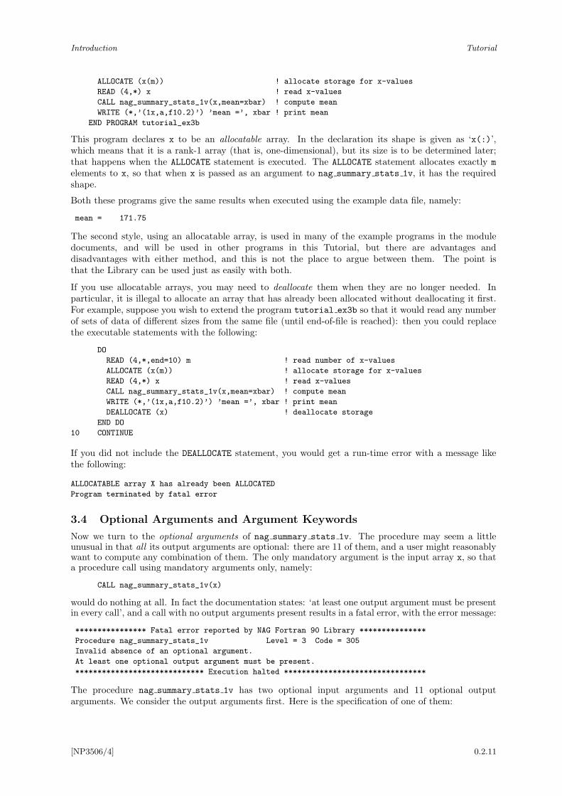
ALLOCATE (x(m)) ! allocate storage for x-values
READ (4,*) x ! read x-values
CALL nag_summary_stats_1v(x,mean=xbar) ! compute mean
WRITE (*,’(1x,a,f10.2)’) ’mean =’, xbar ! print mean
END PROGRAM tutorial_ex3b
This program declares x to be an allocatable array. In the declaration its shape is given as ‘x(:)’,which means that it is a rank-1 array (that is, one-dimensional), but its size is to be determined later;that happens when the ALLOCATE statement is executed. The ALLOCATE statement allocates exactly m
elements to x, so that when x is passed as an argument to nag summary stats 1v, it has the requiredshape.
Both these programs give the same results when executed using the example data file, namely:
mean = 171.75
The second style, using an allocatable array, is used in many of the example programs in the moduledocuments, and will be used in other programs in this Tutorial, but there are advantages anddisadvantages with either method, and this is not the place to argue between them. The point isthat the Library can be used just as easily with both.
If you use allocatable arrays, you may need to deallocate them when they are no longer needed. Inparticular, it is illegal to allocate an array that has already been allocated without deallocating it first.For example, suppose you wish to extend the program tutorial ex3b so that it would read any numberof sets of data of different sizes from the same file (until end-of-file is reached): then you could replacethe executable statements with the following:
DO
READ (4,*,end=10) m ! read number of x-values
ALLOCATE (x(m)) ! allocate storage for x-values
READ (4,*) x ! read x-values
CALL nag_summary_stats_1v(x,mean=xbar) ! compute mean
WRITE (*,’(1x,a,f10.2)’) ’mean =’, xbar ! print mean
DEALLOCATE (x) ! deallocate storage
END DO
10 CONTINUE
If you did not include the DEALLOCATE statement, you would get a run-time error with a message likethe following:
ALLOCATABLE array X has already been ALLOCATED
Program terminated by fatal error
3.4 Optional Arguments and Argument Keywords
Now we turn to the optional arguments of nag summary stats 1v. The procedure may seem a littleunusual in that all its output arguments are optional: there are 11 of them, and a user might reasonablywant to compute any combination of them. The only mandatory argument is the input array x, so thata procedure call using mandatory arguments only, namely:
CALL nag_summary_stats_1v(x)
would do nothing at all. In fact the documentation states: ‘at least one output argument must be presentin every call’, and a call with no output arguments present results in a fatal error, with the error message:
**************** Fatal error reported by NAG Fortran 90 Library ***************
Procedure nag_summary_stats_1v Level = 3 Code = 305
Invalid absence of an optional argument.
At least one optional output argument must be present.
***************************** Execution halted ********************************
The procedure nag summary stats 1v has two optional input arguments and 11 optional outputarguments. We consider the output arguments first. Here is the specification of one of them:
[NP3506/4] 0.2.11
Tutorial Introduction
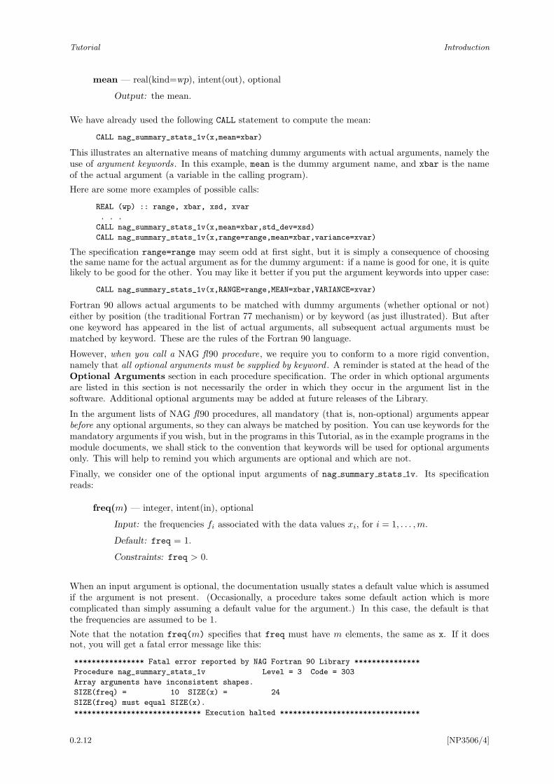
mean — real(kind=wp), intent(out), optional
Output: the mean.
We have already used the following CALL statement to compute the mean:
CALL nag_summary_stats_1v(x,mean=xbar)
This illustrates an alternative means of matching dummy arguments with actual arguments, namely theuse of argument keywords. In this example, mean is the dummy argument name, and xbar is the nameof the actual argument (a variable in the calling program).
Here are some more examples of possible calls:
REAL (wp) :: range, xbar, xsd, xvar
. . .
CALL nag_summary_stats_1v(x,mean=xbar,std_dev=xsd)
CALL nag_summary_stats_1v(x,range=range,mean=xbar,variance=xvar)
The specification range=range may seem odd at first sight, but it is simply a consequence of choosingthe same name for the actual argument as for the dummy argument: if a name is good for one, it is quitelikely to be good for the other. You may like it better if you put the argument keywords into upper case:
CALL nag_summary_stats_1v(x,RANGE=range,MEAN=xbar,VARIANCE=xvar)
Fortran 90 allows actual arguments to be matched with dummy arguments (whether optional or not)either by position (the traditional Fortran 77 mechanism) or by keyword (as just illustrated). But afterone keyword has appeared in the list of actual arguments, all subsequent actual arguments must bematched by keyword. These are the rules of the Fortran 90 language.
However, when you call a NAG fl90 procedure, we require you to conform to a more rigid convention,namely that all optional arguments must be supplied by keyword . A reminder is stated at the head of theOptional Arguments section in each procedure specification. The order in which optional argumentsare listed in this section is not necessarily the order in which they occur in the argument list in thesoftware. Additional optional arguments may be added at future releases of the Library.
In the argument lists of NAG fl90 procedures, all mandatory (that is, non-optional) arguments appearbefore any optional arguments, so they can always be matched by position. You can use keywords for themandatory arguments if you wish, but in the programs in this Tutorial, as in the example programs in themodule documents, we shall stick to the convention that keywords will be used for optional argumentsonly. This will help to remind you which arguments are optional and which are not.
Finally, we consider one of the optional input arguments of nag summary stats 1v. Its specificationreads:
freq(m) — integer, intent(in), optional
Input: the frequencies fi associated with the data values xi, for i = 1, . . . ,m.
Default: freq = 1.
Constraints: freq > 0.
When an input argument is optional, the documentation usually states a default value which is assumedif the argument is not present. (Occasionally, a procedure takes some default action which is morecomplicated than simply assuming a default value for the argument.) In this case, the default is thatthe frequencies are assumed to be 1.
Note that the notation freq(m) specifies that freq must have m elements, the same as x. If it doesnot, you will get a fatal error message like this:
**************** Fatal error reported by NAG Fortran 90 Library ***************
Procedure nag_summary_stats_1v Level = 3 Code = 303
Array arguments have inconsistent shapes.
SIZE(freq) = 10 SIZE(x) = 24
SIZE(freq) must equal SIZE(x).
***************************** Execution halted ********************************
0.2.12 [NP3506/4]
Introduction Tutorial
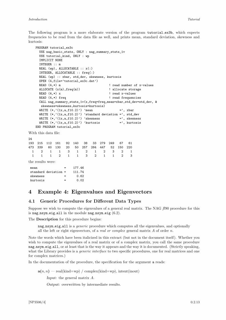
The following program is a more elaborate version of the program tutorial ex3b, which expectsfrequencies to be read from the data file as well, and prints mean, standard deviation, skewness andkurtosis:
PROGRAM tutorial_ex3c
USE nag_basic_stats, ONLY : nag_summary_stats_1v
USE tutorial_kind, ONLY : wp
IMPLICIT NONE
INTEGER :: m
REAL (wp), ALLOCATABLE :: x(:)
INTEGER, ALLOCATABLE :: freq(:)
REAL (wp) :: xbar, std_dev, skewness, kurtosis
OPEN (4,file=’tutorial_ex3c.dat’)
READ (4,*) m ! read number of x-values
ALLOCATE (x(m),freq(m)) ! allocate storage
READ (4,*) x ! read x-values
READ (4,*) freq ! read frequencies
CALL nag_summary_stats_1v(x,freq=freq,mean=xbar,std_dev=std_dev, &
skewness=skewness,kurtosis=kurtosis)
WRITE (*,’(1x,a,f10.2)’) ’mean =’, xbar
WRITE (*,’(1x,a,f10.2)’) ’standard deviation =’, std_dev
WRITE (*,’(1x,a,f10.2)’) ’skewness =’, skewness
WRITE (*,’(1x,a,f10.2)’) ’kurtosis =’, kurtosis
END PROGRAM tutorial_ex3c
With this data file:
24
193 215 112 161 92 140 38 33 279 249 67 61
473 339 60 130 20 50 257 284 447 52 150 220
1 2 1 1 3 1 2 1 2 3 2 1
1 1 1 2 1 1 3 2 1 1 2 3
the results were:
mean = 177.46
standard deviation = 111.74
skewness = 0.62
kurtosis = 0.02
4 Example 4: Eigenvalues and Eigenvectors
4.1 Generic Procedures for Different Data Types
Suppose we wish to compute the eigenvalues of a general real matrix. The NAG fl90 procedure for thisis nag nsym eig all in the module nag nsym eig (6.2).
The Description for this procedure begins:
nag nsym eig all is a generic procedure which computes all the eigenvalues, and optionallyall the left or right eigenvectors, of a real or complex general matrix A of order n.
Note the words which have been italicized in this extract (but not in the document itself). Whether youwish to compute the eigenvalues of a real matrix or of a complex matrix, you call the same procedurenag nsym eig all, or at least that is the way it appears and the way it is documented. (Strictly speaking,what the Library provides is a generic interface to two specific procedures, one for real matrices and onefor complex matrices.)
In the documentation of the procedure, the specification for the argument a reads:
a(n, n) — real(kind=wp) / complex(kind=wp), intent(inout)
Input: the general matrix A.
Output: overwritten by intermediate results.
[NP3506/4] 0.2.13
Tutorial Introduction
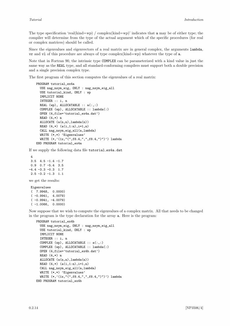
The type specification ‘real(kind=wp) / complex(kind=wp)’ indicates that a may be of either type; thecompiler will determine from the type of the actual argument which of the specific procedures (for realor complex matrices) should be called.
Since the eigenvalues and eigenvectors of a real matrix are in general complex, the arguments lambda,vr and vl of this procedure are always of type complex(kind=wp) whatever the type of a.
Note that in Fortran 90, the intrinsic type COMPLEX can be parameterized with a kind value in just thesame way as the REAL type, and all standard-conforming compilers must support both a double precisionand a single precision complex type.
The first program of this section computes the eigenvalues of a real matrix:
PROGRAM tutorial_ex4a
USE nag_nsym_eig, ONLY : nag_nsym_eig_all
USE tutorial_kind, ONLY : wp
IMPLICIT NONE
INTEGER :: i, n
REAL (wp), ALLOCATABLE :: a(:,:)
COMPLEX (wp), ALLOCATABLE :: lambda(:)
OPEN (4,file=’tutorial_ex4a.dat’)
READ (4,*) n
ALLOCATE (a(n,n),lambda(n))
READ (4,*) (a(i,1:n),i=1,n)
CALL nag_nsym_eig_all(a,lambda)
WRITE (*,*) ’Eigenvalues’
WRITE (*,’(1x,"(",f8.4,",",f8.4,")")’) lambda
END PROGRAM tutorial_ex4a
If we supply the following data file tutorial ex4a.dat
4
3.5 4.5 -1.4 -1.7
0.9 0.7 -5.4 3.5
-4.4 -3.3 -0.3 1.7
2.5 -3.2 -1.3 1.1
we get the results:
Eigenvalues
( 7.9948, 0.0000)
( -0.9941, 4.0079)
( -0.9941, -4.0079)
( -1.0066, 0.0000)
Now suppose that we wish to compute the eigenvalues of a complex matrix. All that needs to be changedin the program is the type declaration for the array a. Here is the program:
PROGRAM tutorial_ex4b
USE nag_nsym_eig, ONLY : nag_nsym_eig_all
USE tutorial_kind, ONLY : wp
IMPLICIT NONE
INTEGER :: i, n
COMPLEX (wp), ALLOCATABLE :: a(:,:)
COMPLEX (wp), ALLOCATABLE :: lambda(:)
OPEN (4,file=’tutorial_ex4b.dat’)
READ (4,*) n
ALLOCATE (a(n,n),lambda(n))
READ (4,*) (a(i,1:n),i=1,n)
CALL nag_nsym_eig_all(a,lambda)
WRITE (*,*) ’Eigenvalues’
WRITE (*,’(1x,"(",f8.4,",",f8.4,")")’) lambda
END PROGRAM tutorial_ex4b
0.2.14 [NP3506/4]
Introduction Tutorial
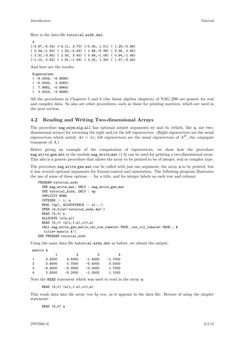
Here is the data file tutorial ex4b.dat:
4
(-3.97,-5.04) (-4.11, 3.70) (-0.34, 1.01) ( 1.29,-0.86)
( 0.34,-1.50) ( 1.52,-0.43) ( 1.88,-5.38) ( 3.36, 0.65)
( 3.31,-3.85) ( 2.50, 3.45) ( 0.88,-1.08) ( 0.64,-1.48)
(-1.10, 0.82) ( 1.81,-1.59) ( 3.25, 1.33) ( 1.57,-3.44)
And here are the results:
Eigenvalues
( -6.0004, -6.9998)
( -5.0000, 2.0060)
( 7.9982, -0.9964)
( 3.0023, -3.9998)
All the procedures in Chapters 5 and 6 (the linear algebra chapters) of NAG fl90 are generic for realand complex data. So also are other procedures, such as those for printing matrices, which are used inthe next section.
4.2 Reading and Writing Two-dimensional Arrays
The procedure nag nsym eig all has optional output arguments vr and vl (which, like a, are two-dimensional arrays) for returning the right and/or the left eigenvectors. (Right eigenvectors are the usualeigenvectors which satisfy Ax = λx; left eigenvectors are the usual eigenvectors of AH , the conjugatetranspose of A.)
Before giving an example of the computation of eigenvectors, we show how the procedurenag write gen mat in the module nag write mat (1.3) can be used for printing a two-dimensional array.This also is a generic procedure that allows the array to be printed to be of integer, real or complex type.
The procedure nag write gen mat can be called with just one argument, the array a to be printed, butit has several optional arguments for format-control and annotation. The following program illustratesthe use of some of these options — for a title, and for integer labels on each row and column:
PROGRAM tutorial_ex4c
USE nag_write_mat, ONLY : nag_write_gen_mat
USE tutorial_kind, ONLY : wp
IMPLICIT NONE
INTEGER :: i, n
REAL (wp), ALLOCATABLE :: a(:,:)
OPEN (4,file=’tutorial_ex4a.dat’)
READ (4,*) n
ALLOCATE (a(n,n))
READ (4,*) (a(i,1:n),i=1,n)
CALL nag_write_gen_mat(a,int_row_labels=.TRUE.,int_col_labels=.TRUE., &
title=’matrix A’)
END PROGRAM tutorial_ex4c
Using the same data file tutorial ex4a.dat as before, we obtain the output:
matrix A
1 2 3 4
1 3.5000 4.5000 -1.4000 -1.7000
2 0.9000 0.7000 -5.4000 3.5000
3 -4.4000 -3.3000 -0.3000 1.7000
4 2.5000 -3.2000 -1.3000 1.1000
Note the READ statement which was used to read in the array a:
READ (4,*) (a(i,1:n),i=1,n)
This reads data into the array row by row , as it appears in the data file. Beware of using the simplerstatement:
READ (4,*) a
[NP3506/4] 0.2.15
Tutorial Introduction
This would read data into the array column by column, so the first record of the data file (the first row ofthe matrix) would be read into the first column of the array, and so on: the effect would be to transposethe array.
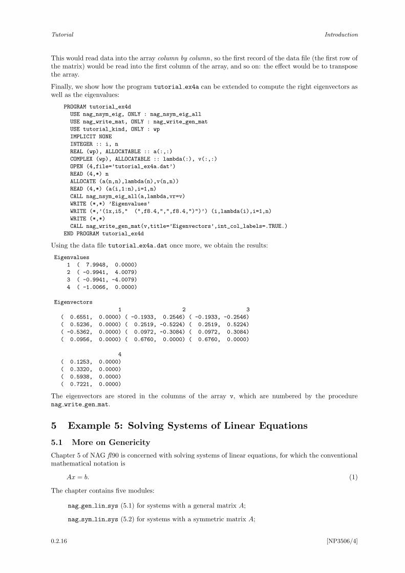
Finally, we show how the program tutorial ex4a can be extended to compute the right eigenvectors aswell as the eigenvalues:
PROGRAM tutorial_ex4d
USE nag_nsym_eig, ONLY : nag_nsym_eig_all
USE nag_write_mat, ONLY : nag_write_gen_mat
USE tutorial_kind, ONLY : wp
IMPLICIT NONE
INTEGER :: i, n
REAL (wp), ALLOCATABLE :: a(:,:)
COMPLEX (wp), ALLOCATABLE :: lambda(:), v(:,:)
OPEN (4,file=’tutorial_ex4a.dat’)
READ (4,*) n
ALLOCATE (a(n,n),lambda(n),v(n,n))
READ (4,*) (a(i,1:n),i=1,n)
CALL nag_nsym_eig_all(a,lambda,vr=v)
WRITE (*,*) ’Eigenvalues’
WRITE (*,’(1x,i5," (",f8.4,",",f8.4,")")’) (i,lambda(i),i=1,n)
WRITE (*,*)
CALL nag_write_gen_mat(v,title=’Eigenvectors’,int_col_labels=.TRUE.)
END PROGRAM tutorial_ex4d
Using the data file tutorial ex4a.dat once more, we obtain the results:
Eigenvalues
1 ( 7.9948, 0.0000)
2 ( -0.9941, 4.0079)
3 ( -0.9941, -4.0079)
4 ( -1.0066, 0.0000)
Eigenvectors
1 2 3
( 0.6551, 0.0000) ( -0.1933, 0.2546) ( -0.1933, -0.2546)
( 0.5236, 0.0000) ( 0.2519, -0.5224) ( 0.2519, 0.5224)
( -0.5362, 0.0000) ( 0.0972, -0.3084) ( 0.0972, 0.3084)
( 0.0956, 0.0000) ( 0.6760, 0.0000) ( 0.6760, 0.0000)
4
( 0.1253, 0.0000)
( 0.3320, 0.0000)
( 0.5938, 0.0000)
( 0.7221, 0.0000)
The eigenvectors are stored in the columns of the array v, which are numbered by the procedurenag write gen mat.
5 Example 5: Solving Systems of Linear Equations
5.1 More on Genericity
Chapter 5 of NAG fl90 is concerned with solving systems of linear equations, for which the conventionalmathematical notation is
Ax = b. (1)
The chapter contains five modules:
nag gen lin sys (5.1) for systems with a general matrix A;
nag sym lin sys (5.2) for systems with a symmetric matrix A;
0.2.16 [NP3506/4]
Introduction Tutorial
nag tri lin sys (5.3) for systems with a triangular matrix A.
nag gen bnd lin sys (5.4) for systems with a general banded matrix A;
nag sym bnd lin sys (5.5) for systems with a symmetric banded matrix A;
In this Tutorial we will illustrate the use of the procedure nag gen lin sol from the modulenag gen lin sys, but if you have a system with a symmetric, triangular or banded matrix, it is preferableto use a procedure from one of the other modules, which will be more efficient and possibly more reliable.
The procedure nag gen lin sol is a generic procedure which can handle either real or complex systems,like the procedure nag nsym eig all which was discussed in Section 4. It is also generic in anotherrespect.
Users often wish to solve several systems with the same matrix A, but with different right-hand sides bi
and different solutions xi:
Axi = bi for i = 1, . . . , r,
which can be rewritten in matrix notation
AX = B, (2)
the columns of B being the right-hand side vectors bi, and the columns of X being the solution vectorsxi.
For solving systems of the form (1), it is convenient to store the right-hand side vector b in a one-dimensional array (an array of rank 1 in Fortran 90 terminology); for solving systems of the form (2),it is convenient to store the matrix B in a two-dimensional array (an array of rank 2). The procedurenag gen lin sol allows for both these possibilities through its generic interface.
Note that if a dummy argument is an assumed-shape array, the actual argument which matches it musthave the same rank: an array of rank 1 — declared, for example, as x(n)— is not equivalent to an arrayof rank 2 with one of its dimensions equal to 1 — declared as x(1,n) or x(n,1). However, NAG fl90avoids any inconvenience which this rule of the language might cause, by providing a generic interfaceand thus allowing either a rank-1 or a rank-2 array to be supplied as the actual argument.
For procedures with a considerable degree of genericity, the Usage section of the proceduredocumentation contains a section on Interfaces, which for nag gen lin sol reads as follows.
Distinct interfaces are provided for each of the four combinations of the following cases:
Real / complex data
Real data: a and b are of type real(kind=wp).
Complex data: a and b are of type complex(kind=wp).
One / many right-hand sidesOne r.h.s.: b is a rank-1 array, and the optional arguments bwd err and fwd err are
scalars.Many r.h.s.: b is a rank-2 array, and the optional arguments bwd err and fwd err are
rank-1 arrays.
Thus the generic interface for nag gen lin sol provides access to four specific procedures, all coveredby a single procedure specification.
The specification of the argument b takes the form:
[NP3506/4] 0.2.17
Tutorial Introduction
b(n) / b(n, r) — real(kind=wp) / complex(kind=wp), intent(inout)
Input: the right-hand side vector b or matrix B.
Output: overwritten on exit by the solution vector x or matrix X.
Constraints: b must be of the same type as a.
Note: if optional error bounds are requested then the solution returned is that computedby iterative refinement.
Note that the stated constraint forbids arbitrary combinations of arguments: you cannot call theprocedure with real a and complex b. If you try to, you will get an error message at compile time;from the NAGWare f90 compiler it will be:
Error: No specific match for reference to generic NAG_GEN_LIN_SOL at line ...
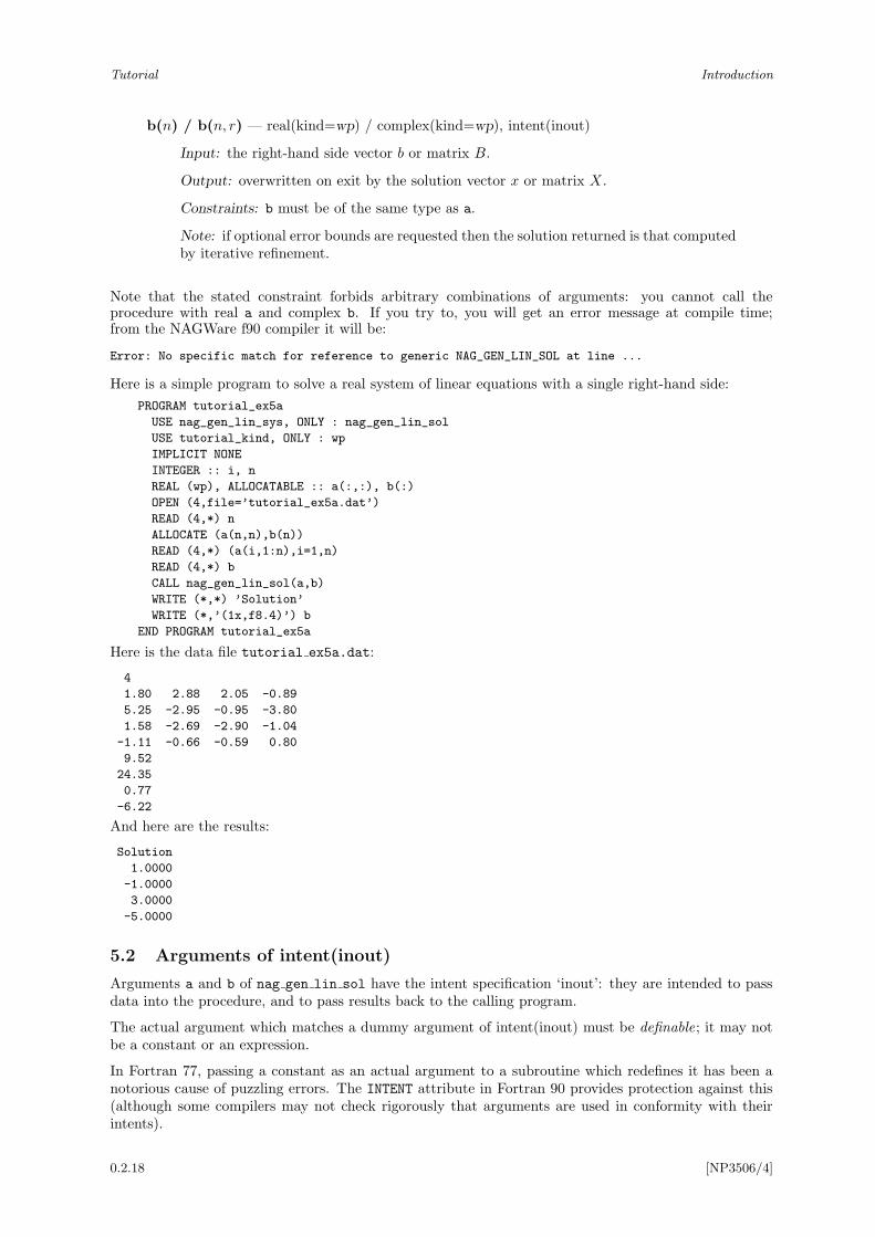
Here is a simple program to solve a real system of linear equations with a single right-hand side:
PROGRAM tutorial_ex5a
USE nag_gen_lin_sys, ONLY : nag_gen_lin_sol
USE tutorial_kind, ONLY : wp
IMPLICIT NONE
INTEGER :: i, n
REAL (wp), ALLOCATABLE :: a(:,:), b(:)
OPEN (4,file=’tutorial_ex5a.dat’)
READ (4,*) n
ALLOCATE (a(n,n),b(n))
READ (4,*) (a(i,1:n),i=1,n)
READ (4,*) b
CALL nag_gen_lin_sol(a,b)
WRITE (*,*) ’Solution’
WRITE (*,’(1x,f8.4)’) b
END PROGRAM tutorial_ex5a
Here is the data file tutorial ex5a.dat:
4
1.80 2.88 2.05 -0.89
5.25 -2.95 -0.95 -3.80
1.58 -2.69 -2.90 -1.04
-1.11 -0.66 -0.59 0.80
9.52
24.35
0.77
-6.22
And here are the results:
Solution
1.0000
-1.0000
3.0000
-5.0000
5.2 Arguments of intent(inout)
Arguments a and b of nag gen lin sol have the intent specification ‘inout’: they are intended to passdata into the procedure, and to pass results back to the calling program.
The actual argument which matches a dummy argument of intent(inout) must be definable; it may notbe a constant or an expression.
In Fortran 77, passing a constant as an actual argument to a subroutine which redefines it has been anotorious cause of puzzling errors. The INTENT attribute in Fortran 90 provides protection against this(although some compilers may not check rigorously that arguments are used in conformity with theirintents).
0.2.18 [NP3506/4]
Introduction Tutorial
In NAG fl90, arguments of intent(inout) are either arrays or structures, which to some extent reduces therisk of supplying a constant or expression. But Fortran 90 allows array constants or array expressions.
Suppose, for example, that you wish to solve the system of equations
|A|x = b,
where |A| denotes the matrix with elements |aij |. You might be tempted to replace the call tonag gen lin sol by
CALL nag_gen_lin_sol(ABS(a),b)
The NAGWare compiler detects this as an error at compile time, giving the message:
Error: No specific match for reference to generic NAG_GEN_LIN_SOL at line 12
because the actual argument ABS(a) cannot be matched with the dummy argument a that hasintent(inout).
Instead, you must assign ABS(a) to another array of the same shape, and then pass this as the argument:
aa = ABS(a)
CALL nag_gen_lin_sol(aa,b)
5.3 Sensitivity of Numerical Results
Although the main purpose of this Tutorial is to teach readers about aspects of the Fortran 90 language,a few remarks will be made here about the sensitivity of numerical results.
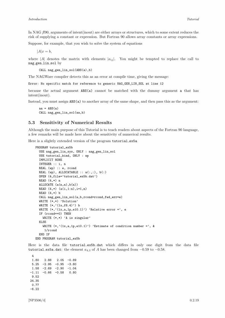
Here is a slightly extended version of the program tutorial ex5a
PROGRAM tutorial_ex5b
USE nag_gen_lin_sys, ONLY : nag_gen_lin_sol
USE tutorial_kind, ONLY : wp
IMPLICIT NONE
INTEGER :: i, n
REAL (wp) :: e, rcond
REAL (wp), ALLOCATABLE :: a(:,:), b(:)
OPEN (4,file=’tutorial_ex5b.dat’)
READ (4,*) n
ALLOCATE (a(n,n),b(n))
READ (4,*) (a(i,1:n),i=1,n)
READ (4,*) b
CALL nag_gen_lin_sol(a,b,rcond=rcond,fwd_err=e)
WRITE (*,*) ’Solution’
WRITE (*,’(1x,f8.4)’) b
WRITE (*,’(1x,a,1p,e10.1)’) ’Relative error =’, e
IF (rcond==0) THEN
WRITE (*,*) ’A is singular’
ELSE
WRITE (*,’(1x,a,1p,e10.1)’) ’Estimate of condition number =’, &
1/rcond
END IF
END PROGRAM tutorial_ex5b
Here is the data file tutorial ex5b.dat which differs in only one digit from the data filetutorial ex5a.dat: the element a4,3 of A has been changed from −0.59 to −0.58.
4
1.80 2.88 2.05 -0.89
5.25 -2.95 -0.95 -3.80
1.58 -2.69 -2.90 -1.04
-1.11 -0.66 -0.58 0.80
9.52
24.35
0.77
-6.22
[NP3506/4] 0.2.19
Tutorial Introduction
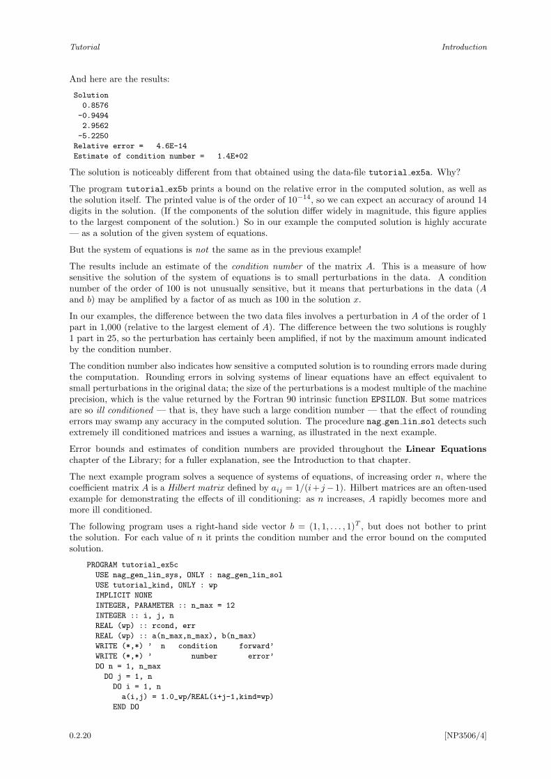
And here are the results:
Solution
0.8576
-0.9494
2.9562
-5.2250
Relative error = 4.6E-14
Estimate of condition number = 1.4E+02
The solution is noticeably different from that obtained using the data-file tutorial ex5a. Why?
The program tutorial ex5b prints a bound on the relative error in the computed solution, as well asthe solution itself. The printed value is of the order of 10−14, so we can expect an accuracy of around 14digits in the solution. (If the components of the solution differ widely in magnitude, this figure appliesto the largest component of the solution.) So in our example the computed solution is highly accurate— as a solution of the given system of equations.
But the system of equations is not the same as in the previous example!
The results include an estimate of the condition number of the matrix A. This is a measure of howsensitive the solution of the system of equations is to small perturbations in the data. A conditionnumber of the order of 100 is not unusually sensitive, but it means that perturbations in the data (Aand b) may be amplified by a factor of as much as 100 in the solution x.
In our examples, the difference between the two data files involves a perturbation in A of the order of 1part in 1,000 (relative to the largest element of A). The difference between the two solutions is roughly1 part in 25, so the perturbation has certainly been amplified, if not by the maximum amount indicatedby the condition number.
The condition number also indicates how sensitive a computed solution is to rounding errors made duringthe computation. Rounding errors in solving systems of linear equations have an effect equivalent tosmall perturbations in the original data; the size of the perturbations is a modest multiple of the machineprecision, which is the value returned by the Fortran 90 intrinsic function EPSILON. But some matricesare so ill conditioned — that is, they have such a large condition number — that the effect of roundingerrors may swamp any accuracy in the computed solution. The procedure nag gen lin sol detects suchextremely ill conditioned matrices and issues a warning, as illustrated in the next example.
Error bounds and estimates of condition numbers are provided throughout the Linear Equationschapter of the Library; for a fuller explanation, see the Introduction to that chapter.
The next example program solves a sequence of systems of equations, of increasing order n, where thecoefficient matrix A is a Hilbert matrix defined by aij = 1/(i+ j−1). Hilbert matrices are an often-usedexample for demonstrating the effects of ill conditioning: as n increases, A rapidly becomes more andmore ill conditioned.
The following program uses a right-hand side vector b = (1, 1, . . . , 1)T , but does not bother to printthe solution. For each value of n it prints the condition number and the error bound on the computedsolution.
PROGRAM tutorial_ex5c
USE nag_gen_lin_sys, ONLY : nag_gen_lin_sol
USE tutorial_kind, ONLY : wp
IMPLICIT NONE
INTEGER, PARAMETER :: n_max = 12
INTEGER :: i, j, n
REAL (wp) :: rcond, err
REAL (wp) :: a(n_max,n_max), b(n_max)
WRITE (*,*) ’ n condition forward’
WRITE (*,*) ’ number error’
DO n = 1, n_max
DO j = 1, n
DO i = 1, n
a(i,j) = 1.0_wp/REAL(i+j-1,kind=wp)
END DO
0.2.20 [NP3506/4]
Introduction Tutorial
END DO
b(1:n) = 1.0_wp
CALL nag_gen_lin_sol(a(1:n,1:n),b(1:n),rcond=rcond,fwd_err=err)
WRITE (*,’(1x,i3,1p,3e12.1)’) n, 1.0_wp/rcond, err
END DO
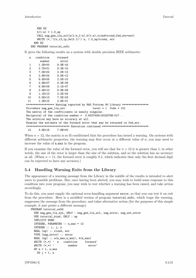
END PROGRAM tutorial_ex5c
It gives the following results on a system with double precision IEEE arithmetic:
n condition forward
number error
1 1.0E+00 8.9E-16
2 2.7E+01 9.3E-15
3 7.5E+02 2.0E-13
4 2.8E+04 6.6E-12
5 9.4E+05 2.0E-10
6 2.9E+07 6.0E-09
7 9.9E+08 2.1E-07
8 3.4E+10 6.9E-06
9 1.1E+12 2.2E-04
10 3.5E+13 7.5E-03
11 1.2E+15 2.6E-01
****************** Warning reported by NAG Fortran 90 Library *****************
Procedure nag_gen_lin_sol Level = 1 Code = 101
The matrix of the coefficients is nearly singular.
Reciprocal of the condition number = 2.632742811818276E-017 .
The solution may have no accuracy at all.
Examine the estimate of the forward error that may be returned in fwd_err.
**************************** Execution continued ******************************
12 3.8E+16 7.8E+00
When n = 12, the matrix is so ill conditioned that the procedure has issued a warning. On systems withdifferent arithmetic properties, the warning may first occur at a different value of n; you may need toincrease the value of n max in the program.
If you examine the value of the forward error, you will see that for n = 12 it is greater than 1; in otherwords, the size of the error is larger than the size of the solution, and so the solution has no accuracyat all. (When n = 11, the forward error is roughly 0.1, which indicates that only the first decimal digitcan be expected to have any accuracy.)
5.4 Handling Warning Exits from the Library
The appearance of a warning message from the Library in the middle of the results is intended to alertusers to possible problems. But, once having been alerted, you may wish to build some response to thiscondition into your program; you may wish to test whether a warning has been raised, and take actionaccordingly.
To do this, you must supply the optional error-handling argument error, so that you can test it on exitfrom the procedure. Here is a modified version of program tutorial ex5c, which traps the warning,suppresses the message from the procedure, and takes alternative action (for the purposes of this simpleexample, it just prints a different message).
PROGRAM tutorial_ex5d
USE nag_gen_lin_sys, ONLY : nag_gen_lin_sol, nag_error, nag_set_error
USE tutorial_kind, ONLY : wp
IMPLICIT NONE
INTEGER, PARAMETER :: n_max = 12
INTEGER :: i, j, n
REAL (wp) :: rcond, err
TYPE (nag_error) :: error
REAL (wp) :: a(n_max,n_max), b(n_max)
WRITE (*,*) ’ n condition forward’
WRITE (*,*) ’ number error’
DO n = 1, n_max
DO j = 1, n
[NP3506/4] 0.2.21
Tutorial Introduction
DO i = 1, n
a(i,j) = 1.0_wp/REAL(i+j-1,kind=wp)
END DO
END DO
b(1:n) = 1.0_wp
CALL nag_set_error(error,print_level=2)
CALL nag_gen_lin_sol(a(1:n,1:n),b(1:n),rcond=rcond,fwd_err=err, &
error=error)
SELECT CASE (error%level)
CASE DEFAULT
WRITE (*,’(1x,i3,1p,3e12.1)’) n, 1.0_wp/rcond, err
CASE (1)
WRITE (*,’(1x,i3,a)’) n, ’ singular to working precision’
CASE (2:)
WRITE (*,’(1x,a)’) ’ Other errors’
END SELECT
END DO
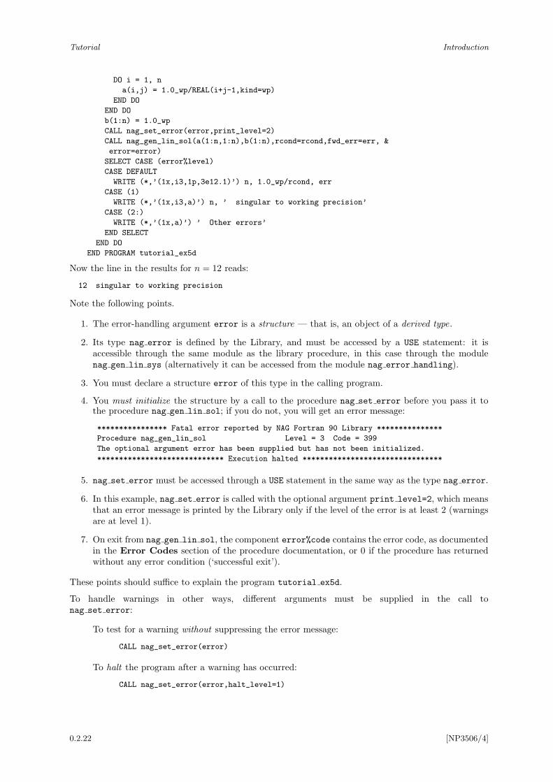
END PROGRAM tutorial_ex5d
Now the line in the results for n = 12 reads:
12 singular to working precision
Note the following points.
1. The error-handling argument error is a structure — that is, an object of a derived type.
2. Its type nag error is defined by the Library, and must be accessed by a USE statement: it isaccessible through the same module as the library procedure, in this case through the modulenag gen lin sys (alternatively it can be accessed from the module nag error handling).
3. You must declare a structure error of this type in the calling program.
4. You must initialize the structure by a call to the procedure nag set error before you pass it tothe procedure nag gen lin sol; if you do not, you will get an error message:
**************** Fatal error reported by NAG Fortran 90 Library ***************
Procedure nag_gen_lin_sol Level = 3 Code = 399
The optional argument error has been supplied but has not been initialized.
***************************** Execution halted ********************************
5. nag set error must be accessed through a USE statement in the same way as the type nag error.
6. In this example, nag set error is called with the optional argument print level=2, which meansthat an error message is printed by the Library only if the level of the error is at least 2 (warningsare at level 1).
7. On exit from nag gen lin sol, the component error%code contains the error code, as documentedin the Error Codes section of the procedure documentation, or 0 if the procedure has returnedwithout any error condition (‘successful exit’).
These points should suffice to explain the program tutorial ex5d.
To handle warnings in other ways, different arguments must be supplied in the call tonag set error:
To test for a warning without suppressing the error message:
CALL nag_set_error(error)
To halt the program after a warning has occurred:
CALL nag_set_error(error,halt_level=1)
0.2.22 [NP3506/4]
Introduction Tutorial
The values of halt level and print level which are supplied as optional arguments to nag set error
are stored as components of the structure error; if they are not present, the default values are halt level
= 2 and print level = 1.
Each error detected by a NAG fl90 procedure has a designated level, stated in the documentation, andequal to the first digit of its error code. If an error is detected, the procedure prints an error message ifthe error has a level ≥ print level, and then halts the program if it has a level ≥ halt level.
On return from the procedure, the error code and the level are stored in the components code and levelof the structure error, and may be tested, as shown in program tutorial ex5d.
6 Example 6: Finding a Solution of a Single NonlinearEquation
6.1 A First Look at Procedure Arguments
The module nag nlin eqn (10.2) contains a single procedure nag nlin eqn sol, which finds a solutionof an equation of the following form:
f(x) = 0 where x ∈ [a, b].
The function f(x) may be any continuous function which is defined on the interval [a, b] and which hasopposite signs at the end-points a and b; this guarantees that the function has at least one zero in theinterval.
In order to use nag nlin eqn sol to find a solution of such an equation, the function f(x) must bedefined by a function subprogram, which you (the user) must supply. This function is passed as anargument to nag nlin eqn sol.
For our example, we will solve the equation
ex = 3x2 where x ∈ [0, 3],
which must be expressed as:
f(x) ≡ ex − 3x2 = 0. (3)
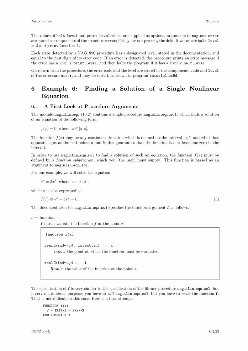
The documentation for nag nlin eqn sol specifies the function argument f as follows:
f — function
f must evaluate the function f at the point x.
function f(x)
real(kind=wp), intent(in) :: x
Input: the point at which the function must be evaluated.
real(kind=wp) :: f
Result: the value of the function at the point x.
The specification of f is very similar to the specification of the library procedure nag nlin eqn sol, butit serves a different purpose: you have to call nag nlin eqn sol, but you have to write the function f.That is not difficult in this case. Here is a first attempt:
FUNCTION f(x)
f = EXP(x) - 3*x**2
END FUNCTION f
[NP3506/4] 0.2.23
Tutorial Introduction
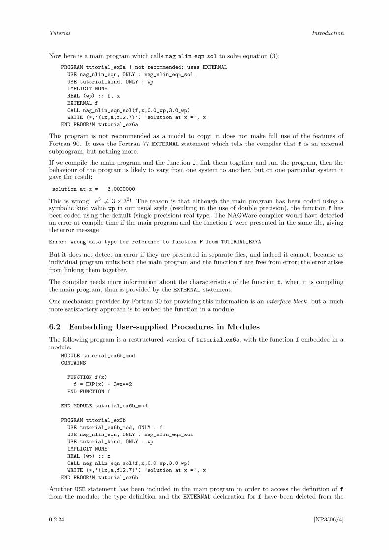
Now here is a main program which calls nag nlin eqn sol to solve equation (3):
PROGRAM tutorial_ex6a ! not recommended: uses EXTERNAL
USE nag_nlin_eqn, ONLY : nag_nlin_eqn_sol
USE tutorial_kind, ONLY : wp
IMPLICIT NONE
REAL (wp) :: f, x
EXTERNAL f
CALL nag_nlin_eqn_sol(f,x,0.0_wp,3.0_wp)
WRITE (*,’(1x,a,f12.7)’) ’solution at x =’, x
END PROGRAM tutorial_ex6a
This program is not recommended as a model to copy; it does not make full use of the features ofFortran 90. It uses the Fortran 77 EXTERNAL statement which tells the compiler that f is an externalsubprogram, but nothing more.
If we compile the main program and the function f, link them together and run the program, then thebehaviour of the program is likely to vary from one system to another, but on one particular system itgave the result:
solution at x = 3.0000000
This is wrong! e3 6= 3 × 32! The reason is that although the main program has been coded using asymbolic kind value wp in our usual style (resulting in the use of double precision), the function f hasbeen coded using the default (single precision) real type. The NAGWare compiler would have detectedan error at compile time if the main program and the function f were presented in the same file, givingthe error message
Error: Wrong data type for reference to function F from TUTORIAL_EX7A
But it does not detect an error if they are presented in separate files, and indeed it cannot, because asindividual program units both the main program and the function f are free from error; the error arisesfrom linking them together.
The compiler needs more information about the characteristics of the function f, when it is compilingthe main program, than is provided by the EXTERNAL statement.
One mechanism provided by Fortran 90 for providing this information is an interface block , but a muchmore satisfactory approach is to embed the function in a module.
6.2 Embedding User-supplied Procedures in Modules
The following program is a restructured version of tutorial ex6a, with the function f embedded in amodule:
MODULE tutorial_ex6b_mod
CONTAINS
FUNCTION f(x)
f = EXP(x) - 3*x**2
END FUNCTION f
END MODULE tutorial_ex6b_mod
PROGRAM tutorial_ex6b
USE tutorial_ex6b_mod, ONLY : f
USE nag_nlin_eqn, ONLY : nag_nlin_eqn_sol
USE tutorial_kind, ONLY : wp
IMPLICIT NONE
REAL (wp) :: x
CALL nag_nlin_eqn_sol(f,x,0.0_wp,3.0_wp)
WRITE (*,’(1x,a,f12.7)’) ’solution at x =’, x
END PROGRAM tutorial_ex6b
Another USE statement has been included in the main program in order to access the definition of ffrom the module; the type definition and the EXTERNAL declaration for f have been deleted from the
0.2.24 [NP3506/4]
Introduction Tutorial
main program. (In technical terms, the function f has been converted from an external procedure into amodule procedure.)
The program tutorial ex6b will still not be correct for use with a double precision implementation ofthe Library, but now the error can be detected at compile-time. The NAGWare f90 compiler gives thefamiliar message:
Error: No specific match for reference to generic NAG_NLIN_EQN_SOL at line 16
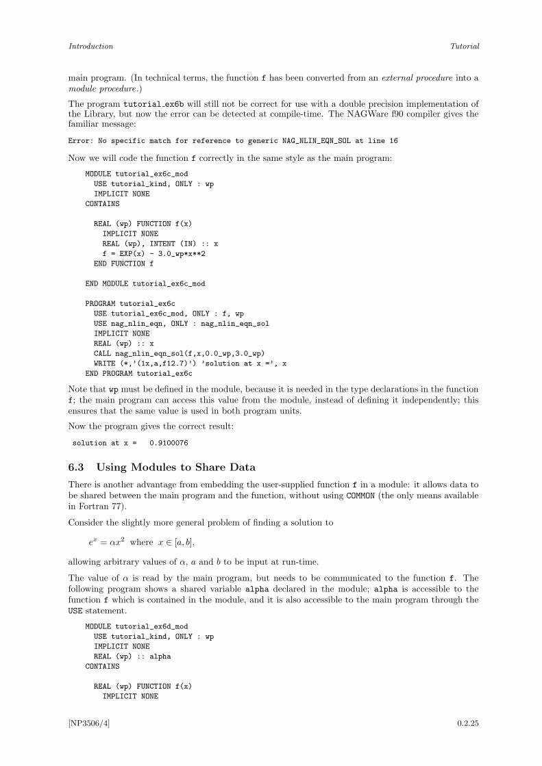
Now we will code the function f correctly in the same style as the main program:
MODULE tutorial_ex6c_mod
USE tutorial_kind, ONLY : wp
IMPLICIT NONE
CONTAINS
REAL (wp) FUNCTION f(x)
IMPLICIT NONE
REAL (wp), INTENT (IN) :: x
f = EXP(x) - 3.0_wp*x**2
END FUNCTION f
END MODULE tutorial_ex6c_mod
PROGRAM tutorial_ex6c
USE tutorial_ex6c_mod, ONLY : f, wp
USE nag_nlin_eqn, ONLY : nag_nlin_eqn_sol
IMPLICIT NONE
REAL (wp) :: x
CALL nag_nlin_eqn_sol(f,x,0.0_wp,3.0_wp)
WRITE (*,’(1x,a,f12.7)’) ’solution at x =’, x
END PROGRAM tutorial_ex6c
Note that wp must be defined in the module, because it is needed in the type declarations in the functionf; the main program can access this value from the module, instead of defining it independently; thisensures that the same value is used in both program units.
Now the program gives the correct result:
solution at x = 0.9100076
6.3 Using Modules to Share Data
There is another advantage from embedding the user-supplied function f in a module: it allows data tobe shared between the main program and the function, without using COMMON (the only means availablein Fortran 77).
Consider the slightly more general problem of finding a solution to
ex = αx2 where x ∈ [a, b],
allowing arbitrary values of α, a and b to be input at run-time.
The value of α is read by the main program, but needs to be communicated to the function f. Thefollowing program shows a shared variable alpha declared in the module; alpha is accessible to thefunction f which is contained in the module, and it is also accessible to the main program through theUSE statement.
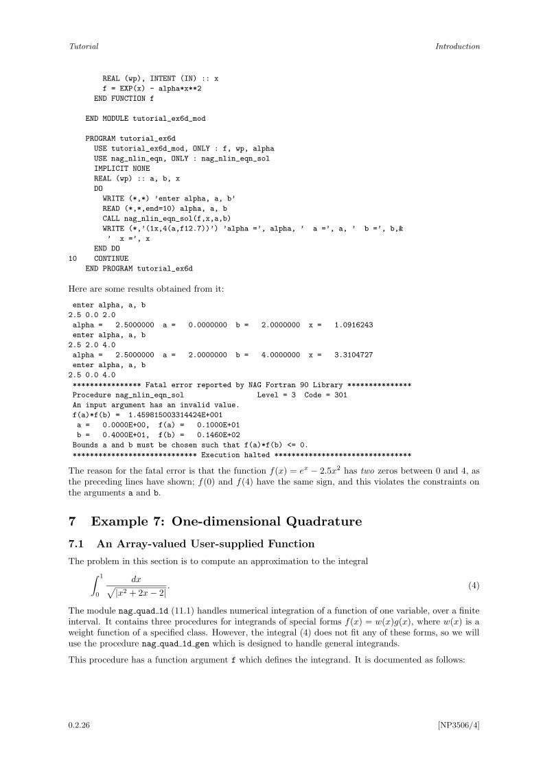
MODULE tutorial_ex6d_mod
USE tutorial_kind, ONLY : wp
IMPLICIT NONE
REAL (wp) :: alpha
CONTAINS
REAL (wp) FUNCTION f(x)
IMPLICIT NONE
[NP3506/4] 0.2.25
Tutorial Introduction
REAL (wp), INTENT (IN) :: x
f = EXP(x) - alpha*x**2
END FUNCTION f
END MODULE tutorial_ex6d_mod
PROGRAM tutorial_ex6d
USE tutorial_ex6d_mod, ONLY : f, wp, alpha
USE nag_nlin_eqn, ONLY : nag_nlin_eqn_sol
IMPLICIT NONE
REAL (wp) :: a, b, x
DO
WRITE (*,*) ’enter alpha, a, b’
READ (*,*,end=10) alpha, a, b
CALL nag_nlin_eqn_sol(f,x,a,b)
WRITE (*,’(1x,4(a,f12.7))’) ’alpha =’, alpha, ’ a =’, a, ’ b =’, b,&
’ x =’, x
END DO
10 CONTINUE
END PROGRAM tutorial_ex6d
Here are some results obtained from it:
enter alpha, a, b
2.5 0.0 2.0
alpha = 2.5000000 a = 0.0000000 b = 2.0000000 x = 1.0916243
enter alpha, a, b
2.5 2.0 4.0
alpha = 2.5000000 a = 2.0000000 b = 4.0000000 x = 3.3104727
enter alpha, a, b
2.5 0.0 4.0
**************** Fatal error reported by NAG Fortran 90 Library ***************
Procedure nag_nlin_eqn_sol Level = 3 Code = 301
An input argument has an invalid value.
f(a)*f(b) = 1.459815003314424E+001
a = 0.0000E+00, f(a) = 0.1000E+01
b = 0.4000E+01, f(b) = 0.1460E+02
Bounds a and b must be chosen such that f(a)*f(b) <= 0.
***************************** Execution halted ********************************
The reason for the fatal error is that the function f(x) = ex − 2.5x2 has two zeros between 0 and 4, asthe preceding lines have shown; f(0) and f(4) have the same sign, and this violates the constraints onthe arguments a and b.
7 Example 7: One-dimensional Quadrature
7.1 An Array-valued User-supplied Function
The problem in this section is to compute an approximation to the integral
∫ 1
0
dx√
|x2 + 2x− 2|. (4)
The module nag quad 1d (11.1) handles numerical integration of a function of one variable, over a finiteinterval. It contains three procedures for integrands of special forms f(x) = w(x)g(x), where w(x) is aweight function of a specified class. However, the integral (4) does not fit any of these forms, so we willuse the procedure nag quad 1d gen which is designed to handle general integrands.
This procedure has a function argument f which defines the integrand. It is documented as follows:
0.2.26 [NP3506/4]
Introduction Tutorial
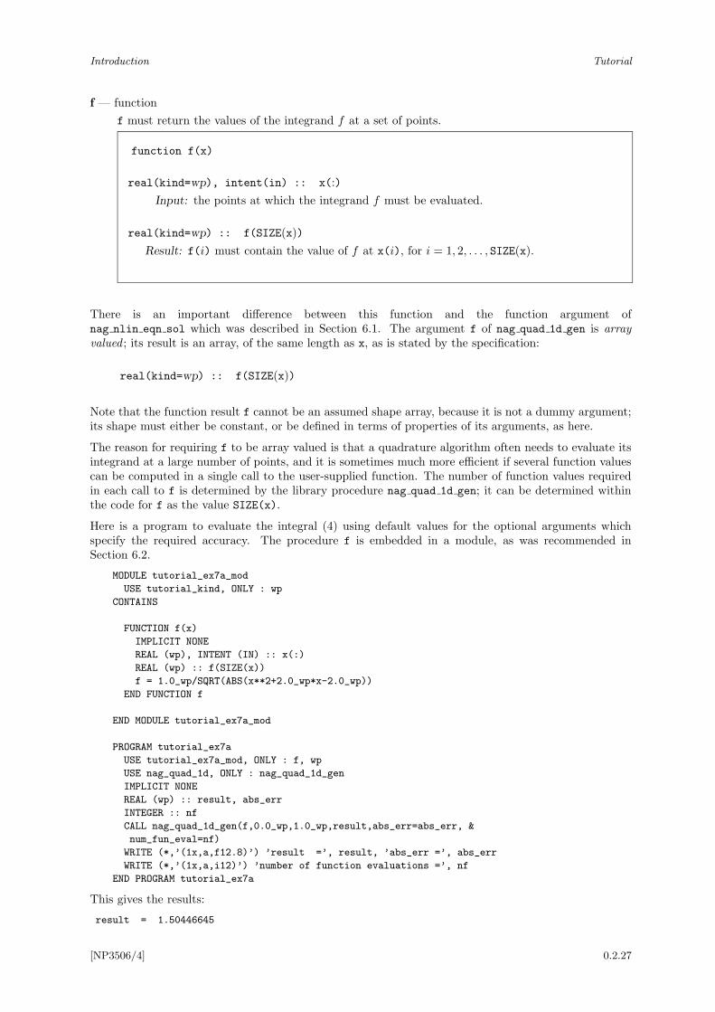
f — function
f must return the values of the integrand f at a set of points.
function f(x)
real(kind=wp), intent(in) :: x(:)
Input: the points at which the integrand f must be evaluated.
real(kind=wp) :: f(SIZE(x))
Result: f(i) must contain the value of f at x(i), for i = 1, 2, . . . , SIZE(x).
There is an important difference between this function and the function argument ofnag nlin eqn sol which was described in Section 6.1. The argument f of nag quad 1d gen is arrayvalued ; its result is an array, of the same length as x, as is stated by the specification:
real(kind=wp) :: f(SIZE(x))
Note that the function result f cannot be an assumed shape array, because it is not a dummy argument;its shape must either be constant, or be defined in terms of properties of its arguments, as here.
The reason for requiring f to be array valued is that a quadrature algorithm often needs to evaluate itsintegrand at a large number of points, and it is sometimes much more efficient if several function valuescan be computed in a single call to the user-supplied function. The number of function values requiredin each call to f is determined by the library procedure nag quad 1d gen; it can be determined withinthe code for f as the value SIZE(x).
Here is a program to evaluate the integral (4) using default values for the optional arguments whichspecify the required accuracy. The procedure f is embedded in a module, as was recommended inSection 6.2.
MODULE tutorial_ex7a_mod
USE tutorial_kind, ONLY : wp
CONTAINS
FUNCTION f(x)
IMPLICIT NONE
REAL (wp), INTENT (IN) :: x(:)
REAL (wp) :: f(SIZE(x))
f = 1.0_wp/SQRT(ABS(x**2+2.0_wp*x-2.0_wp))
END FUNCTION f
END MODULE tutorial_ex7a_mod
PROGRAM tutorial_ex7a
USE tutorial_ex7a_mod, ONLY : f, wp
USE nag_quad_1d, ONLY : nag_quad_1d_gen
IMPLICIT NONE
REAL (wp) :: result, abs_err
INTEGER :: nf
CALL nag_quad_1d_gen(f,0.0_wp,1.0_wp,result,abs_err=abs_err, &
num_fun_eval=nf)
WRITE (*,’(1x,a,f12.8)’) ’result =’, result, ’abs_err =’, abs_err
WRITE (*,’(1x,a,i12)’) ’number of function evaluations =’, nf
END PROGRAM tutorial_ex7a
This gives the results:
result = 1.50446645
[NP3506/4] 0.2.27

Tutorial Introduction
abs_err = 0.00008186
number of function evaluations = 903
The code for the function f does not look at first sight as if it is array valued. The statement
f = 1.0_wp/SQRT(ABS(x**2+2.0_wp*x-2.0_wp))
is identical to the statement that you would write for a scalar-valued function with a scalar argument.But on the right-hand side of the assignment, x is an array, so the arithmetic expressions are array valued,and the intrinsic functions SQRT and ABS are elemental , which means that they return an array-valuedresult if their arguments are arrays. And finally f on the left-hand side of the assignment is an array, sothe statement as a whole is an array assignment. It is equivalent to:
DO i = 1, SIZE(x)
f(i) = 1.0_wp/SQRT(ABS(x(i)**2+2.0_wp*x(i)-2.0_wp))
END DO
A DO-loop would be essential if the expression for f(x) involved other functions that are not array valued.
7.2 Handling Failure Exits from the Library
Now suppose that we wish to investigate the effect of specifying different values for the requested accuracy.Since the value of the integral is close to 1, absolute and relative accuracy have roughly the same meaning.We will set the relative accuracy rel acc to zero, which means that only absolute accuracy is operative.
The following program requests a progressively more accurate result, setting abs acc to 10−3, 10−4, . . . :
MODULE tutorial_ex7b_mod
USE tutorial_kind, ONLY : wp
CONTAINS
FUNCTION f(x)
IMPLICIT NONE
REAL (wp), INTENT (IN) :: x(:)
REAL (wp) :: f(SIZE(x))
f = 1.0_wp/SQRT(ABS(x**2+2.0_wp*x-2.0_wp))
END FUNCTION f
END MODULE tutorial_ex7b_mod
PROGRAM tutorial_ex7b
USE tutorial_ex7b_mod, ONLY : f, wp
USE nag_quad_1d, ONLY : nag_quad_1d_gen
IMPLICIT NONE
INTEGER :: i, nf
REAL (wp) :: result, abs_err, abs_acc
WRITE (6,*) ’ requested result estimated number of’
WRITE (6,*) ’ accuracy accuracy evaluations’
DO i = 3, 10
abs_acc = 10.0_wp**(-i)
CALL nag_quad_1d_gen(f,0.0_wp,1.0_wp,result,abs_acc=abs_acc, &
rel_acc=0.0_wp,abs_err=abs_err,num_fun_eval=nf)
WRITE (*,’(1x,3f12.8,i12)’) abs_acc, result, abs_err, nf
END DO
END PROGRAM tutorial_ex7b
The results are:
requested result estimated number of
accuracy accuracy evaluations
0.00100000 1.50439172 0.00075447 819
0.00010000 1.50446645 0.00008186 903
0.00001000 1.50460652 0.00000114 1197
0.00000100 1.50462235 0.00000005 1743
0.00000010 1.50462235 0.00000005 1827
****************** Failure reported by NAG Fortran 90 Library *****************
0.2.28 [NP3506/4]
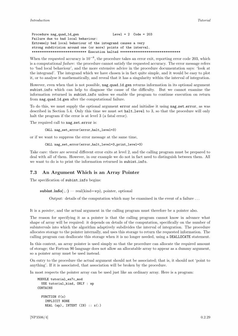
Introduction Tutorial
Procedure nag_quad_1d_gen Level = 2 Code = 203
Failure due to bad local behaviour:
Extremely bad local behaviour of the integrand causes a very
strong subdivision around one (or more) points of the interval.
***************************** Execution halted ********************************
When the requested accuracy is 10−8, the procedure takes an error exit, reporting error code 203, whichis a computational failure: the procedure cannot satisfy the requested accuracy. The error message refersto ‘bad local behaviour’, and the more extensive advice in the procedure documentation says: ‘look atthe integrand’. The integrand which we have chosen is in fact quite simple, and it would be easy to plotit, or to analyse it mathematically, and reveal that it has a singularity within the interval of integration.
However, even when that is not possible, nag quad 1d gen returns information in its optional argumentsubint info which can help to diagnose the cause of the difficulty. But we cannot examine theinformation returned in subint info unless we enable the program to continue execution on returnfrom nag quad 1d gen after the computational failure.
To do this, we must supply the optional argument error and initialise it using nag set error, as wasdescribed in Section 5.4. Only this time we must set halt level to 3, so that the procedure will onlyhalt the program if the error is at level 3 (a fatal error).
The required call to nag set error is:
CALL nag_set_error(error,halt_level=3)
or if we want to suppress the error message at the same time,
CALL nag_set_error(error,halt_level=3,print_level=3)
Take care: there are several different error exits at level 2, and the calling program must be prepared todeal with all of them. However, in our example we do not in fact need to distinguish between them. Allwe want to do is to print the information returned in subint info.
7.3 An Argument Which is an Array Pointer
The specification of subint info begins:
subint info(:, :) — real(kind=wp), pointer, optional
Output: details of the computation which may be examined in the event of a failure . . .
It is a pointer , and the actual argument in the calling program must therefore be a pointer also.
The reason for specifying it as a pointer is that the calling program cannot know in advance whatshape of array will be required: it depends on details of the computation, specifically on the number ofsubintervals into which the algorithm adaptively subdivides the interval of integration. The procedureallocates storage to the pointer internally, and uses this storage to return the requested information. Thecalling program can deallocate this storage when it is no longer needed, using a DEALLOCATE statement.
In this context, an array pointer is used simply so that the procedure can allocate the required amountof storage; the Fortran 90 language does not allow an allocatable array to appear as a dummy argument,so a pointer array must be used instead.
On entry to the procedure the actual argument should not be associated; that is, it should not ‘point toanything’. If it is associated, that association will be broken by the procedure.
In most respects the pointer array can be used just like an ordinary array. Here is a program:
MODULE tutorial_ex7c_mod
USE tutorial_kind, ONLY : wp
CONTAINS
FUNCTION f(x)
IMPLICIT NONE
REAL (wp), INTENT (IN) :: x(:)
[NP3506/4] 0.2.29
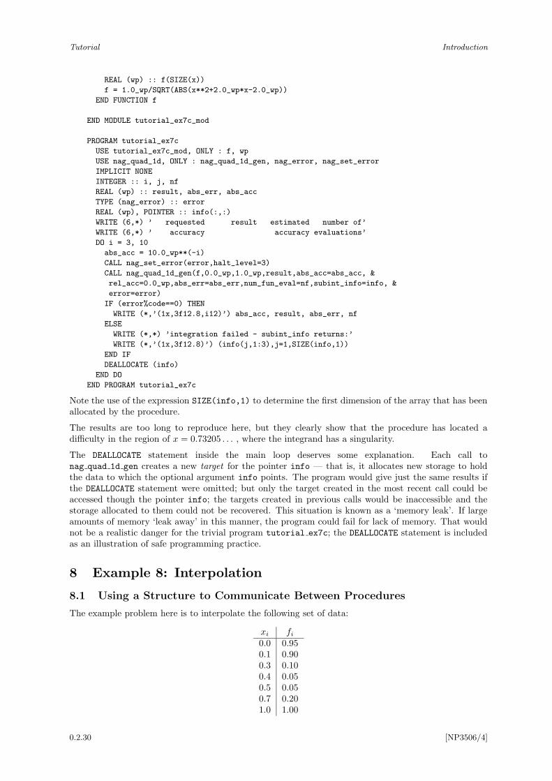
Tutorial Introduction
REAL (wp) :: f(SIZE(x))
f = 1.0_wp/SQRT(ABS(x**2+2.0_wp*x-2.0_wp))
END FUNCTION f
END MODULE tutorial_ex7c_mod
PROGRAM tutorial_ex7c
USE tutorial_ex7c_mod, ONLY : f, wp
USE nag_quad_1d, ONLY : nag_quad_1d_gen, nag_error, nag_set_error
IMPLICIT NONE
INTEGER :: i, j, nf
REAL (wp) :: result, abs_err, abs_acc
TYPE (nag_error) :: error
REAL (wp), POINTER :: info(:,:)
WRITE (6,*) ’ requested result estimated number of’
WRITE (6,*) ’ accuracy accuracy evaluations’
DO i = 3, 10
abs_acc = 10.0_wp**(-i)
CALL nag_set_error(error,halt_level=3)
CALL nag_quad_1d_gen(f,0.0_wp,1.0_wp,result,abs_acc=abs_acc, &
rel_acc=0.0_wp,abs_err=abs_err,num_fun_eval=nf,subint_info=info, &
error=error)
IF (error%code==0) THEN
WRITE (*,’(1x,3f12.8,i12)’) abs_acc, result, abs_err, nf
ELSE
WRITE (*,*) ’integration failed - subint_info returns:’
WRITE (*,’(1x,3f12.8)’) (info(j,1:3),j=1,SIZE(info,1))
END IF
DEALLOCATE (info)
END DO
END PROGRAM tutorial_ex7c
Note the use of the expression SIZE(info,1) to determine the first dimension of the array that has beenallocated by the procedure.
The results are too long to reproduce here, but they clearly show that the procedure has located adifficulty in the region of x = 0.73205 . . . , where the integrand has a singularity.
The DEALLOCATE statement inside the main loop deserves some explanation. Each call tonag quad 1d gen creates a new target for the pointer info — that is, it allocates new storage to holdthe data to which the optional argument info points. The program would give just the same results ifthe DEALLOCATE statement were omitted; but only the target created in the most recent call could beaccessed though the pointer info; the targets created in previous calls would be inaccessible and thestorage allocated to them could not be recovered. This situation is known as a ‘memory leak’. If largeamounts of memory ‘leak away’ in this manner, the program could fail for lack of memory. That wouldnot be a realistic danger for the trivial program tutorial ex7c; the DEALLOCATE statement is includedas an illustration of safe programming practice.
8 Example 8: Interpolation
8.1 Using a Structure to Communicate Between Procedures
The example problem here is to interpolate the following set of data:
xi fi
0.0 0.950.1 0.900.3 0.100.4 0.050.5 0.050.7 0.201.0 1.00
0.2.30 [NP3506/4]
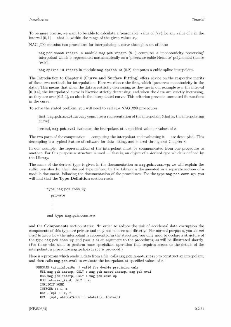
Introduction Tutorial
To be more precise, we want to be able to calculate a ‘reasonable’ value of f(x) for any value of x in theinterval [0, 1] — that is, within the range of the given values xi.
NAG fl90 contains two procedures for interpolating a curve through a set of data:
nag pch monot interp in module nag pch interp (8.1) computes a ‘monotonicity preserving’interpolant which is represented mathematically as a ‘piecewise cubic Hermite’ polynomial (hence‘pch’);
nag spline 1d interp in module nag spline 1d (8.2) computes a cubic spline interpolant.
The Introduction to Chapter 8 (Curve and Surface Fitting) offers advice on the respective meritsof these two methods for interpolation. Here we choose the first, which ‘preserves monotonicity in thedata’. This means that when the data are strictly decreasing, as they are in our example over the interval[0, 0.4], the interpolated curve is likewise strictly decreasing; and when the data are strictly increasing,as they are over [0.5, 1], so also is the interpolated curve. This criterion prevents unwanted fluctuationsin the curve.
To solve the stated problem, you will need to call two NAG fl90 procedures:
first, nag pch monot interp computes a representation of the interpolant (that is, the interpolatingcurve);
second, nag pch eval evaluates the interpolant at a specified value or values of x.
The two parts of the computation — computing the interpolant and evaluating it — are decoupled. Thisdecoupling is a typical feature of software for data fitting, and is used throughout Chapter 8.
In our example, the representation of the interpolant must be communicated from one procedure toanother. For this purpose a structure is used — that is, an object of a derived type which is defined bythe Library.
The name of the derived type is given in the documentation as nag pch comm wp; we will explain thesuffix wp shortly. Each derived type defined by the Library is documented in a separate section of amodule document, following the documentation of the procedures. For the type nag pch comm wp, youwill find that the Type Definition section reads
type nag pch comm wp
private
.
.
.
end type nag pch comm wp
and the Components section states: ‘In order to reduce the risk of accidental data corruption thecomponents of this type are private and may not be accessed directly.’ For normal purposes, you do not
need to know how the interpolant is represented in the structure; you only need to declare a structure ofthe type nag pch comm wp and pass it as an argument to the procedures, as will be illustrated shortly.(For those who want to perform some specialized operation that requires access to the details of theinterpolant, a procedure nag pch extract is provided.)
Here is a program which reads in data from a file, calls nag pch monot interp to construct an interpolant,and then calls nag pch eval to evaluate the interpolant at specified values of x.
PROGRAM tutorial_ex8a ! valid for double precision only
USE nag_pch_interp, ONLY : nag_pch_monot_interp, nag_pch_eval
USE nag_pch_interp, ONLY : nag_pch_comm_dp
USE tutorial_kind, ONLY : wp
IMPLICIT NONE
INTEGER :: i, m
REAL (wp) :: x, f
REAL (wp), ALLOCATABLE :: xdata(:), fdata(:)
[NP3506/4] 0.2.31
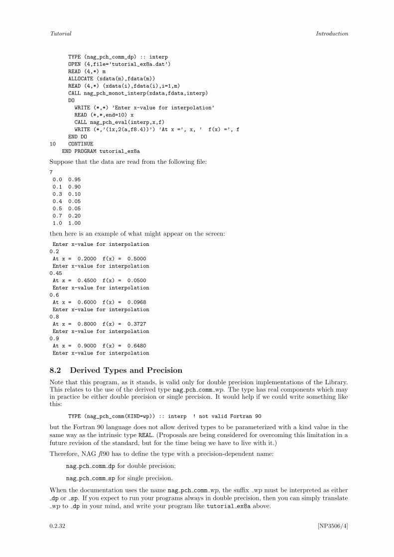
Tutorial Introduction
TYPE (nag_pch_comm_dp) :: interp
OPEN (4,file=’tutorial_ex8a.dat’)
READ (4,*) m
ALLOCATE (xdata(m),fdata(m))
READ (4,*) (xdata(i),fdata(i),i=1,m)
CALL nag_pch_monot_interp(xdata,fdata,interp)
DO
WRITE (*,*) ’Enter x-value for interpolation’
READ (*,*,end=10) x
CALL nag_pch_eval(interp,x,f)
WRITE (*,’(1x,2(a,f8.4))’) ’At x =’, x, ’ f(x) =’, f
END DO
10 CONTINUE
END PROGRAM tutorial_ex8a
Suppose that the data are read from the following file:
7
0.0 0.95
0.1 0.90
0.3 0.10
0.4 0.05
0.5 0.05
0.7 0.20
1.0 1.00
then here is an example of what might appear on the screen:
Enter x-value for interpolation
0.2
At x = 0.2000 f(x) = 0.5000
Enter x-value for interpolation
0.45
At x = 0.4500 f(x) = 0.0500
Enter x-value for interpolation
0.6
At x = 0.6000 f(x) = 0.0968
Enter x-value for interpolation
0.8
At x = 0.8000 f(x) = 0.3727
Enter x-value for interpolation
0.9
At x = 0.9000 f(x) = 0.6480
Enter x-value for interpolation
8.2 Derived Types and Precision
Note that this program, as it stands, is valid only for double precision implementations of the Library.This relates to the use of the derived type nag pch comm wp. The type has real components which mayin practice be either double precision or single precision. It would help if we could write something likethis:
TYPE (nag_pch_comm(KIND=wp)) :: interp ! not valid Fortran 90
but the Fortran 90 language does not allow derived types to be parameterized with a kind value in thesame way as the intrinsic type REAL. (Proposals are being considered for overcoming this limitation in afuture revision of the standard, but for the time being we have to live with it.)
Therefore, NAG fl90 has to define the type with a precision-dependent name:
nag pch comm dp for double precision;
nag pch comm sp for single precision.
When the documentation uses the name nag pch comm wp, the suffix wp must be interpreted as eitherdp or sp. If you expect to run your programs always in double precision, then you can simply translatewp to dp in your mind, and write your program like tutorial ex8a above.
0.2.32 [NP3506/4]
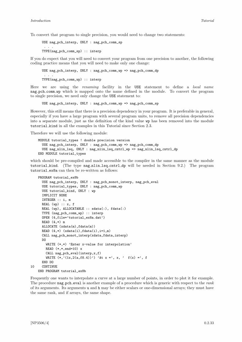
Introduction Tutorial
To convert that program to single precision, you would need to change two statements:
USE nag_pch_interp, ONLY : nag_pch_comm_sp
. . .
TYPE(nag_pch_comm_sp) :: interp
If you do expect that you will need to convert your program from one precision to another, the followingcoding practice means that you will need to make only one change:
USE nag_pch_interp, ONLY : nag_pch_comm_wp => nag_pch_comm_dp
. . .
TYPE(nag_pch_comm_wp) :: interp
Here we are using the renaming facility in the USE statement to define a local namenag pch comm wp which is mapped onto the name defined in the module. To convert the programto single precision, we need only change the USE statement to:
USE nag_pch_interp, ONLY : nag_pch_comm_wp => nag_pch_comm_sp
However, this still means that there is a precision dependency in your program. It is preferable in general,especially if you have a large program with several program units, to remove all precision dependenciesinto a separate module, just as the definition of the kind value wp has been removed into the moduletutorial kind in all the examples in this Tutorial since Section 2.3.
Therefore we will use the following module:
MODULE tutorial_types ! double precision version
USE nag_pch_interp, ONLY : nag_pch_comm_wp => nag_pch_comm_dp
USE nag_nlin_lsq, ONLY : nag_nlin_lsq_cntrl_wp => nag_nlin_lsq_cntrl_dp
END MODULE tutorial_types
which should be pre-compiled and made accessible to the compiler in the same manner as the moduletutorial kind. (The type nag nlin lsq cntrl dp will be needed in Section 9.2.) The programtutorial ex8a can then be re-written as follows:
PROGRAM tutorial_ex8b
USE nag_pch_interp, ONLY : nag_pch_monot_interp, nag_pch_eval
USE tutorial_types, ONLY : nag_pch_comm_wp
USE tutorial_kind, ONLY : wp
IMPLICIT NONE
INTEGER :: i, m
REAL (wp) :: x, f
REAL (wp), ALLOCATABLE :: xdata(:), fdata(:)
TYPE (nag_pch_comm_wp) :: interp
OPEN (4,file=’tutorial_ex8a.dat’)
READ (4,*) m
ALLOCATE (xdata(m),fdata(m))
READ (4,*) (xdata(i),fdata(i),i=1,m)
CALL nag_pch_monot_interp(xdata,fdata,interp)
DO
WRITE (*,*) ’Enter x-value for interpolation’
READ (*,*,end=10) x
CALL nag_pch_eval(interp,x,f)
WRITE (*,’(1x,2(a,f8.4))’) ’At x =’, x, ’ f(x) =’, f
END DO
10 CONTINUE
END PROGRAM tutorial_ex8b
Frequently one wants to interpolate a curve at a large number of points, in order to plot it for example.The procedure nag pch eval is another example of a procedure which is generic with respect to the rankof its arguments. Its arguments u and h may be either scalars or one-dimensional arrays; they must havethe same rank, and if arrays, the same shape.
[NP3506/4] 0.2.33
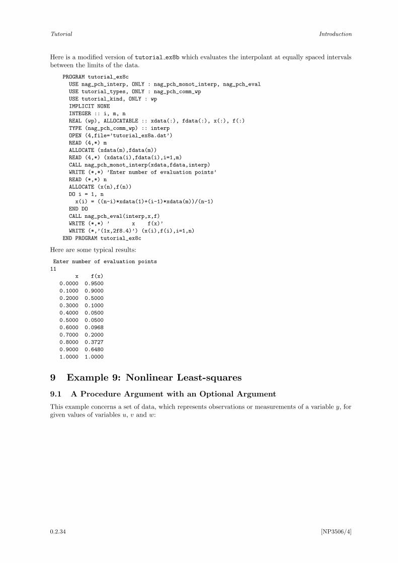
Tutorial Introduction
Here is a modified version of tutorial ex8b which evaluates the interpolant at equally spaced intervalsbetween the limits of the data.
PROGRAM tutorial_ex8c
USE nag_pch_interp, ONLY : nag_pch_monot_interp, nag_pch_eval
USE tutorial_types, ONLY : nag_pch_comm_wp
USE tutorial_kind, ONLY : wp
IMPLICIT NONE
INTEGER :: i, m, n
REAL (wp), ALLOCATABLE :: xdata(:), fdata(:), x(:), f(:)
TYPE (nag_pch_comm_wp) :: interp
OPEN (4,file=’tutorial_ex8a.dat’)
READ (4,*) m
ALLOCATE (xdata(m),fdata(m))
READ (4,*) (xdata(i),fdata(i),i=1,m)
CALL nag_pch_monot_interp(xdata,fdata,interp)
WRITE (*,*) ’Enter number of evaluation points’
READ (*,*) n
ALLOCATE (x(n),f(n))
DO i = 1, n
x(i) = ((n-i)*xdata(1)+(i-1)*xdata(m))/(n-1)
END DO
CALL nag_pch_eval(interp,x,f)
WRITE (*,*) ’ x f(x)’
WRITE (*,’(1x,2f8.4)’) (x(i),f(i),i=1,n)
END PROGRAM tutorial_ex8c
Here are some typical results:
Enter number of evaluation points
11
x f(x)
0.0000 0.9500
0.1000 0.9000
0.2000 0.5000
0.3000 0.1000
0.4000 0.0500
0.5000 0.0500
0.6000 0.0968
0.7000 0.2000
0.8000 0.3727
0.9000 0.6480
1.0000 1.0000
9 Example 9: Nonlinear Least-squares
9.1 A Procedure Argument with an Optional Argument
This example concerns a set of data, which represents observations or measurements of a variable y, forgiven values of variables u, v and w:
0.2.34 [NP3506/4]
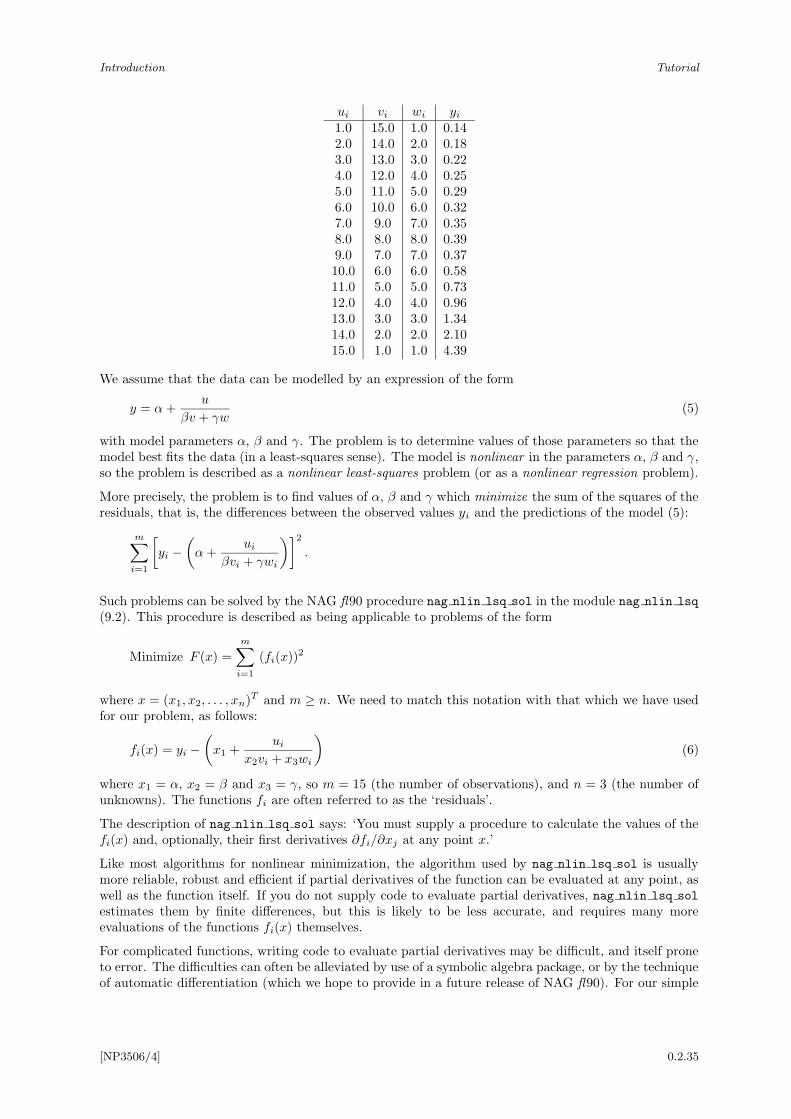
Introduction Tutorial
ui vi wi yi
1.0 15.0 1.0 0.142.0 14.0 2.0 0.183.0 13.0 3.0 0.224.0 12.0 4.0 0.255.0 11.0 5.0 0.296.0 10.0 6.0 0.327.0 9.0 7.0 0.358.0 8.0 8.0 0.399.0 7.0 7.0 0.3710.0 6.0 6.0 0.5811.0 5.0 5.0 0.7312.0 4.0 4.0 0.9613.0 3.0 3.0 1.3414.0 2.0 2.0 2.1015.0 1.0 1.0 4.39
We assume that the data can be modelled by an expression of the form
y = α+u
βv + γw(5)
with model parameters α, β and γ. The problem is to determine values of those parameters so that themodel best fits the data (in a least-squares sense). The model is nonlinear in the parameters α, β and γ,so the problem is described as a nonlinear least-squares problem (or as a nonlinear regression problem).
More precisely, the problem is to find values of α, β and γ which minimize the sum of the squares of theresiduals, that is, the differences between the observed values yi and the predictions of the model (5):
m∑
i=1
[
yi −
(
α+ui
βvi + γwi
)]2
.
Such problems can be solved by the NAG fl90 procedure nag nlin lsq sol in the module nag nlin lsq
(9.2). This procedure is described as being applicable to problems of the form
Minimize F (x) =
m∑
i=1
(fi(x))2
where x = (x1, x2, . . . , xn)T and m ≥ n. We need to match this notation with that which we have used
for our problem, as follows:
fi(x) = yi −
(
x1 +ui
x2vi + x3wi
)
(6)
where x1 = α, x2 = β and x3 = γ, so m = 15 (the number of observations), and n = 3 (the number ofunknowns). The functions fi are often referred to as the ‘residuals’.
The description of nag nlin lsq sol says: ‘You must supply a procedure to calculate the values of thefi(x) and, optionally, their first derivatives ∂fi/∂xj at any point x.’
Like most algorithms for nonlinear minimization, the algorithm used by nag nlin lsq sol is usuallymore reliable, robust and efficient if partial derivatives of the function can be evaluated at any point, aswell as the function itself. If you do not supply code to evaluate partial derivatives, nag nlin lsq sol
estimates them by finite differences, but this is likely to be less accurate, and requires many moreevaluations of the functions fi(x) themselves.
For complicated functions, writing code to evaluate partial derivatives may be difficult, and itself proneto error. The difficulties can often be alleviated by use of a symbolic algebra package, or by the techniqueof automatic differentiation (which we hope to provide in a future release of NAG fl90). For our simple
[NP3506/4] 0.2.35
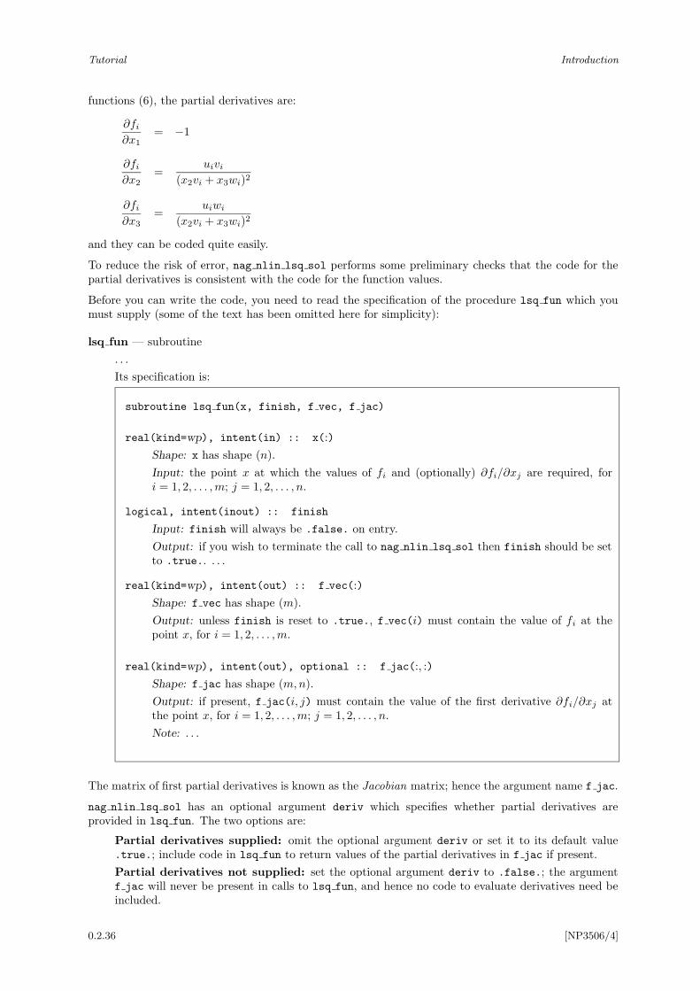
Tutorial Introduction
functions (6), the partial derivatives are:
∂fi
∂x1
= −1
∂fi
∂x2
=uivi
(x2vi + x3wi)2
∂fi
∂x3
=uiwi
(x2vi + x3wi)2
and they can be coded quite easily.
To reduce the risk of error, nag nlin lsq sol performs some preliminary checks that the code for thepartial derivatives is consistent with the code for the function values.
Before you can write the code, you need to read the specification of the procedure lsq fun which youmust supply (some of the text has been omitted here for simplicity):
lsq fun — subroutine
. . .
Its specification is:
subroutine lsq fun(x, finish, f vec, f jac)
real(kind=wp), intent(in) :: x(:)
Shape: x has shape (n).
Input: the point x at which the values of fi and (optionally) ∂fi/∂xj are required, fori = 1, 2, . . . ,m; j = 1, 2, . . . , n.
logical, intent(inout) :: finish
Input: finish will always be .false. on entry.
Output: if you wish to terminate the call to nag nlin lsq sol then finish should be setto .true.. . . .
real(kind=wp), intent(out) :: f vec(:)
Shape: f vec has shape (m).
Output: unless finish is reset to .true., f vec(i) must contain the value of fi at thepoint x, for i = 1, 2, . . . ,m.
real(kind=wp), intent(out), optional :: f jac(:, :)
Shape: f jac has shape (m,n).
Output: if present, f jac(i, j) must contain the value of the first derivative ∂fi/∂xj atthe point x, for i = 1, 2, . . . ,m; j = 1, 2, . . . , n.
Note: . . .
The matrix of first partial derivatives is known as the Jacobian matrix; hence the argument name f jac.
nag nlin lsq sol has an optional argument deriv which specifies whether partial derivatives areprovided in lsq fun. The two options are:
Partial derivatives supplied: omit the optional argument deriv or set it to its default value.true.; include code in lsq fun to return values of the partial derivatives in f jac if present.
Partial derivatives not supplied: set the optional argument deriv to .false.; the argumentf jac will never be present in calls to lsq fun, and hence no code to evaluate derivatives need beincluded.
0.2.36 [NP3506/4]
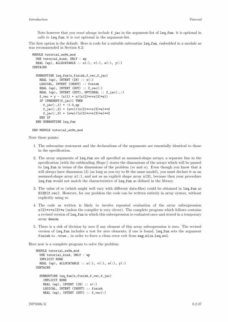
Introduction Tutorial
Note however that you must always include f jac in the argument-list of lsq fun: it is optional incalls to lsq fun; it is not optional in the argument-list.
The first option is the default. Here is code for a suitable subroutine lsq fun, embedded in a module aswas recommended in Section 6.2:
MODULE tutorial_ex9x_mod
USE tutorial_kind, ONLY : wp
REAL (wp), ALLOCATABLE :: u(:), v(:), w(:), y(:)
CONTAINS
SUBROUTINE lsq_fun(x,finish,f_vec,f_jac)
REAL (wp), INTENT (IN) :: x(:)
LOGICAL, INTENT (INOUT) :: finish
REAL (wp), INTENT (OUT) :: f_vec(:)
REAL (wp), INTENT (OUT), OPTIONAL :: f_jac(:,:)
f_vec = y - (x(1) + u/(x(2)*v+x(3)*w))
IF (PRESENT(f_jac)) THEN
f_jac(:,1) = -1.0_wp
f_jac(:,2) = (u*v)/(x(2)*v+x(3)*w)**2
f_jac(:,3) = (u*w)/(x(2)*v+x(3)*w)**2
END IF
END SUBROUTINE lsq_fun
END MODULE tutorial_ex9x_mod
Note these points:
1. The subroutine statement and the declarations of the arguments are essentially identical to thosein the specification.
2. The array arguments of lsq fun are all specified as assumed-shape arrays; a separate line in thespecification (with the subheading Shape:) states the dimensions of the arrays which will be passedto lsq fun in terms of the dimensions of the problem (m and n). Even though you know that xwill always have dimension (3) (as long as you try to fit the same model), you must declare it as anassumed-shape array x(:), and not as an explicit shape array x(3), because then your procedurelsq fun would not match the characteristics of lsq fun as defined in the library.
3. The value of m (which might well vary with different data-files) could be obtained in lsq fun asSIZE(f vec). However, for our problem the code can be written entirely in array syntax, withoutexplicitly using m.
4. The code as written is likely to involve repeated evaluation of the array subexpressionx(2)*v+x(3)*w (unless the compiler is very clever). The complete program which follows containsa revised version of lsq fun in which this subexpression is evaluated once and stored in a temporaryarray denom.
5. There is a risk of division by zero if any element of this array subexpression is zero. The revisedversion of lsq fun includes a test for zero elements; if one is found, lsq fun sets the argumentfinish to .true., in order to force a clean error exit from nag nlin lsq sol.
Here now is a complete program to solve the problem:
MODULE tutorial_ex9a_mod
USE tutorial_kind, ONLY : wp
IMPLICIT NONE
REAL (wp), ALLOCATABLE :: u(:), v(:), w(:), y(:)
CONTAINS
SUBROUTINE lsq_fun(x,finish,f_vec,f_jac)
IMPLICIT NONE
REAL (wp), INTENT (IN) :: x(:)
LOGICAL, INTENT (INOUT) :: finish
REAL (wp), INTENT (OUT) :: f_vec(:)
[NP3506/4] 0.2.37
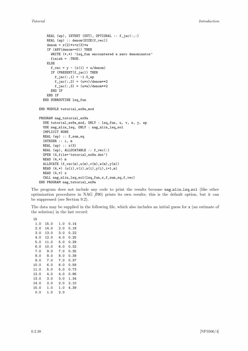
Tutorial Introduction
REAL (wp), INTENT (OUT), OPTIONAL :: f_jac(:,:)
REAL (wp) :: denom(SIZE(f_vec))
denom = x(2)*v+x(3)*w
IF (ANY(denom==0)) THEN
WRITE (*,*) ’lsq_fun encountered a zero denominator’
finish = .TRUE.
ELSE
f_vec = y - (x(1) + u/denom)
IF (PRESENT(f_jac)) THEN
f_jac(:,1) = -1.0_wp
f_jac(:,2) = (u*v)/denom**2
f_jac(:,3) = (u*w)/denom**2
END IF
END IF
END SUBROUTINE lsq_fun
END MODULE tutorial_ex9a_mod
PROGRAM nag_tutorial_ex9a
USE tutorial_ex9a_mod, ONLY : lsq_fun, u, v, w, y, wp
USE nag_nlin_lsq, ONLY : nag_nlin_lsq_sol
IMPLICIT NONE
REAL (wp) :: f_sum_sq
INTEGER :: i, m
REAL (wp) :: x(3)
REAL (wp), ALLOCATABLE :: f_vec(:)
OPEN (4,file=’tutorial_ex9a.dat’)
READ (4,*) m
ALLOCATE (f_vec(m),u(m),v(m),w(m),y(m))
READ (4,*) (u(i),v(i),w(i),y(i),i=1,m)
READ (4,*) x
CALL nag_nlin_lsq_sol(lsq_fun,x,f_sum_sq,f_vec)
END PROGRAM nag_tutorial_ex9a
The program does not include any code to print the results because nag nlin lsq sol (like otheroptimization procedures in NAG fl90) prints its own results; this is the default option, but it canbe suppressed (see Section 9.2).
The data may be supplied in the following file, which also includes an initial guess for x (an estimate ofthe solution) in the last record:
15
1.0 15.0 1.0 0.14
2.0 14.0 2.0 0.18
3.0 13.0 3.0 0.22
4.0 12.0 4.0 0.25
5.0 11.0 5.0 0.29
6.0 10.0 6.0 0.32
7.0 9.0 7.0 0.35
8.0 8.0 8.0 0.39
9.0 7.0 7.0 0.37
10.0 6.0 6.0 0.58
11.0 5.0 5.0 0.73
12.0 4.0 4.0 0.96
13.0 3.0 3.0 1.34
14.0 2.0 2.0 2.10
15.0 1.0 1.0 4.39
0.0 1.0 2.0
0.2.38 [NP3506/4]
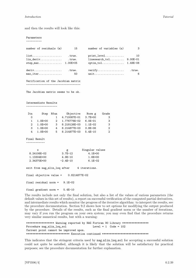
Introduction Tutorial
and then the results will look like this:
Parameters
----------
number of residuals (m) 15 number of variables (n) 3
list................... .true. print_level............ 10
lin_deriv.............. .true. linesearch_tol......... 9.00E-01
step_max............... 1.00E+05 optim_tol.............. 1.49E-08
deriv.................. .true. verify................. .true.
max_iter............... 50 unit................... 6
Verification of the Jacobian matrix
-----------------------------------
The Jacobian matrix seems to be ok.
Intermediate Results
--------------------
Itn Step Nfun Objective Norm g Grade
0 1 4.710087E-01 3.7E+00 3
1 1.0E+00 2 1.776776E-02 6.0E-01 3
2 1.0E+00 3 8.218126E-03 1.1E-02 3
3 1.0E+00 4 8.214877E-03 3.8E-06 2
4 1.0E+00 5 8.214877E-03 5.4E-10 2
Final Result
------------
x g Singular values
8.24106E-02 3.7E-12 4.1E+00
1.13304E+00 4.9E-10 1.6E+00
2.34370E+00 -2.4E-10 6.1E-02
exit from nag_nlin_lsq after 4 iterations.
final objective value = 0.8214877E-02
final residual norm = 9.1E-02
final gradient norm = 5.4E-10
The results include not only the final solution, but also a list of the values of various parameters (thedefault values in this set of results), a report on successful verification of the computed partial derivatives,and intermediate results which monitor the progress of the iterative algorithm: to interpret the results, seethe procedure documentation. Section 9.2 shows how to set options for modifying the output producedby the procedure. Details of the results, such as the final gradient norm or the number of iterations,may vary if you run the program on your own system; you may even find that the procedure returnsvery similar numerical results, but with a warning:
****************** Warning reported by NAG Fortran 90 Library *****************
Procedure nag_nlin_lsq_sol Level = 1 Code = 102
Current point cannot be improved upon.
**************************** Execution continued ******************************
This indicates that the stringent criteria used by nag nlin lsq sol for accepting a successful solutioncould not quite be satisfied, although it is likely that the solution will be satisfactory for practicalpurposes; see the procedure documentation for further explanation.
[NP3506/4] 0.2.39
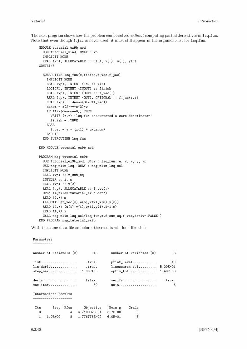
Tutorial Introduction
The next program shows how the problem can be solved without computing partial derivatives in lsq fun.Note that even though f jac is never used, it must still appear in the argument-list for lsq fun.
MODULE tutorial_ex9b_mod
USE tutorial_kind, ONLY : wp
IMPLICIT NONE
REAL (wp), ALLOCATABLE :: u(:), v(:), w(:), y(:)
CONTAINS
SUBROUTINE lsq_fun(x,finish,f_vec,f_jac)
IMPLICIT NONE
REAL (wp), INTENT (IN) :: x(:)
LOGICAL, INTENT (INOUT) :: finish
REAL (wp), INTENT (OUT) :: f_vec(:)
REAL (wp), INTENT (OUT), OPTIONAL :: f_jac(:,:)
REAL (wp) :: denom(SIZE(f_vec))
denom = x(2)*v+x(3)*w
IF (ANY(denom==0)) THEN
WRITE (*,*) ’lsq_fun encountered a zero denominator’
finish = .TRUE.
ELSE
f_vec = y - (x(1) + u/denom)
END IF
END SUBROUTINE lsq_fun
END MODULE tutorial_ex9b_mod
PROGRAM nag_tutorial_ex9b
USE tutorial_ex9b_mod, ONLY : lsq_fun, u, v, w, y, wp
USE nag_nlin_lsq, ONLY : nag_nlin_lsq_sol
IMPLICIT NONE
REAL (wp) :: f_sum_sq
INTEGER :: i, m
REAL (wp) :: x(3)
REAL (wp), ALLOCATABLE :: f_vec(:)
OPEN (4,file=’tutorial_ex9a.dat’)
READ (4,*) m
ALLOCATE (f_vec(m),u(m),v(m),w(m),y(m))
READ (4,*) (u(i),v(i),w(i),y(i),i=1,m)
READ (4,*) x
CALL nag_nlin_lsq_sol(lsq_fun,x,f_sum_sq,f_vec,deriv=.FALSE.)
END PROGRAM nag_tutorial_ex9b
With the same data file as before, the results will look like this:
Parameters
----------
number of residuals (m) 15 number of variables (n) 3
list................... .true. print_level............ 10
lin_deriv.............. .true. linesearch_tol......... 5.00E-01
step_max............... 1.00E+05 optim_tol.............. 1.49E-08
deriv.................. .false. verify................. .true.
max_iter............... 50 unit................... 6
Intermediate Results
--------------------
Itn Step Nfun Objective Norm g Grade
0 4 4.710087E-01 3.7E+00 3
1 1.0E+00 8 1.776776E-02 6.0E-01 3
0.2.40 [NP3506/4]
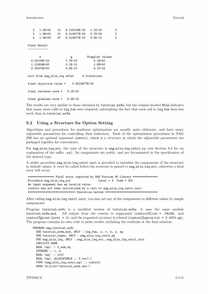
Introduction Tutorial
2 1.0E+00 12 8.218126E-03 1.1E-02 3
3 1.0E+00 21 8.214877E-03 3.7E-06 2
4 1.0E+00 27 8.214877E-03 9.5E-10 2
Final Result
------------
x g Singular values
8.24106E-02 7.7E-10 4.1E+00
1.13304E+00 3.1E-10 1.6E+00
2.34370E+00 4.6E-10 6.1E-02
exit from nag_nlin_lsq after 4 iterations.
final objective value = 0.8214877E-02
final residual norm = 9.1E-02
final gradient norm = 9.5E-10
The results are very similar to those obtained by tutorial ex9a, but the column headed Nfun indicatesthat many more calls to lsq fun were required, outweighing the fact that each call to lsq fun does lesswork than in tutorial ex9a.
9.2 Using a Structure for Option Setting
Algorithms and procedures for nonlinear optimization are usually quite elaborate, and have manyadjustable parameters for controlling their behaviour. Each of the optimization procedures in NAGfl90 has an optional argument control, which is a structure in which the adjustable parameters arepackaged together for convenience.
For nag nlin lsq sol, the type of the structure is nag nlin lsq cntrl wp (see Section 8.2 for anexplanation of the suffix wp). Its components are public, and are documented in the specification ofthe derived type.
A utility procedure nag nlin lsq cntrl init is provided to initialize the components of the structureto default values: it must be called before the structure is passed to nag nlin lsq sol, otherwise a fatalerror will occur:
**************** Fatal error reported by NAG Fortran 90 Library ***************
Procedure nag_nlin_lsq_sol Level = 3 Code = 301
An input argument has an invalid value.
control has not been initialized by a call to nag_nlin_lsq_cntrl_init.
***************************** Execution halted ********************************
After calling nag nlin lsq cntrl init, you may set any of the components to different values by simpleassignments.
Program tutorial ex9c is a modified version of tutorial ex9a; it uses the same moduletutorial ex9a mod. All output from the routine is suppressed (control%list = .FALSE. andcontrol%print level = 0); and the requested accuracy is relaxed (control%optim tol = 0.0001 wp).The program contains its own code to print results, including the residuals at the final solution.
PROGRAM nag_tutorial_ex9c
USE tutorial_ex9a_mod, ONLY : lsq_fun, u, v, w, y, wp
USE tutorial_types, ONLY : nag_nlin_lsq_cntrl_wp
USE nag_nlin_lsq, ONLY : nag_nlin_lsq_sol, nag_nlin_lsq_cntrl_init
IMPLICIT NONE
REAL (wp) :: f_sum_sq
INTEGER :: i, m
REAL (wp) :: x(3)
REAL (wp), ALLOCATABLE :: f_vec(:)
TYPE (nag_nlin_lsq_cntrl_wp) :: control
OPEN (4,file=’tutorial_ex9a.dat’)
[NP3506/4] 0.2.41
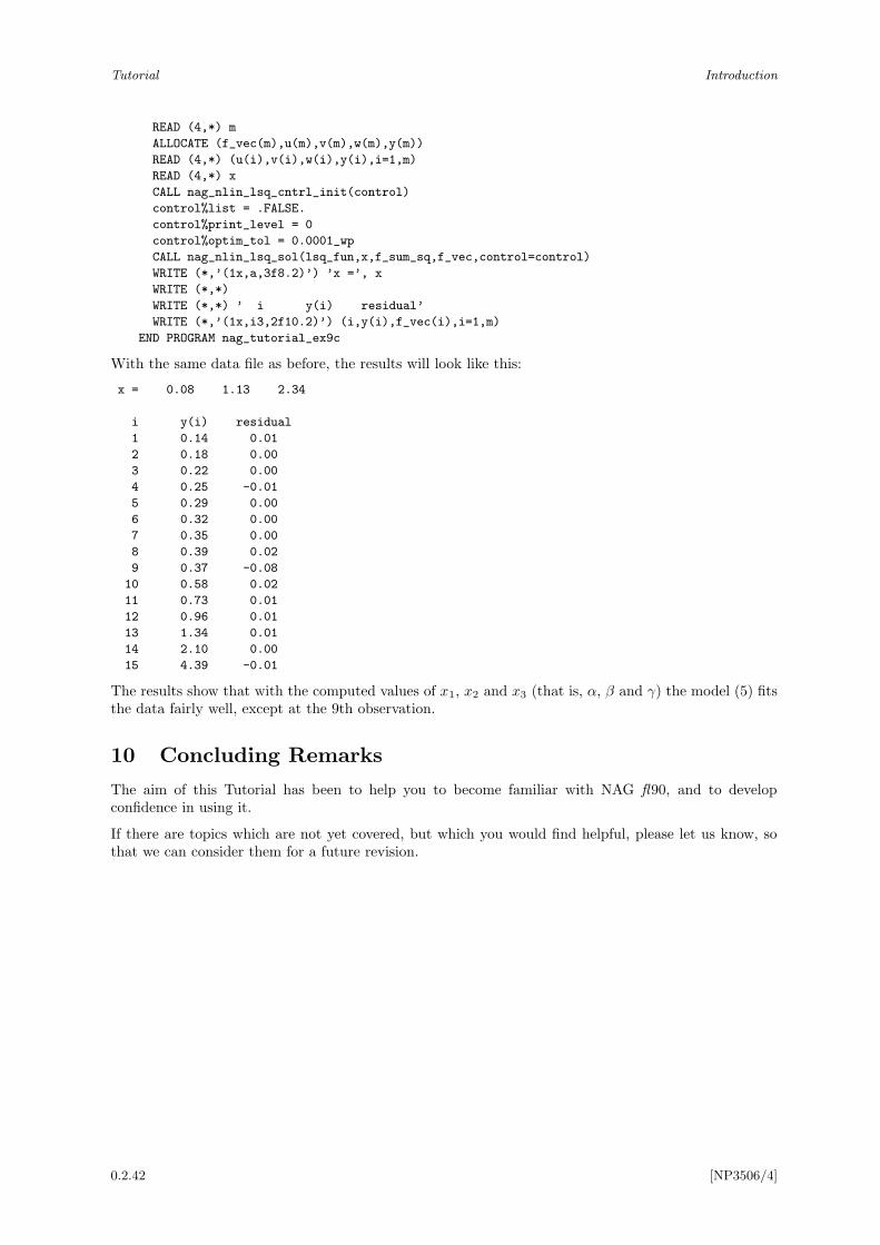
Tutorial Introduction
READ (4,*) m
ALLOCATE (f_vec(m),u(m),v(m),w(m),y(m))
READ (4,*) (u(i),v(i),w(i),y(i),i=1,m)
READ (4,*) x
CALL nag_nlin_lsq_cntrl_init(control)
control%list = .FALSE.
control%print_level = 0
control%optim_tol = 0.0001_wp
CALL nag_nlin_lsq_sol(lsq_fun,x,f_sum_sq,f_vec,control=control)
WRITE (*,’(1x,a,3f8.2)’) ’x =’, x
WRITE (*,*)
WRITE (*,*) ’ i y(i) residual’
WRITE (*,’(1x,i3,2f10.2)’) (i,y(i),f_vec(i),i=1,m)
END PROGRAM nag_tutorial_ex9c
With the same data file as before, the results will look like this:
x = 0.08 1.13 2.34
i y(i) residual
1 0.14 0.01
2 0.18 0.00
3 0.22 0.00
4 0.25 -0.01
5 0.29 0.00
6 0.32 0.00
7 0.35 0.00
8 0.39 0.02
9 0.37 -0.08
10 0.58 0.02
11 0.73 0.01
12 0.96 0.01
13 1.34 0.01
14 2.10 0.00
15 4.39 -0.01
The results show that with the computed values of x1, x2 and x3 (that is, α, β and γ) the model (5) fitsthe data fairly well, except at the 9th observation.
10 Concluding Remarks
The aim of this Tutorial has been to help you to become familiar with NAG fl90, and to developconfidence in using it.
If there are topics which are not yet covered, but which you would find helpful, please let us know, sothat we can consider them for a future revision.
0.2.42 [NP3506/4]