Tutorial: Methods for Reproducible Research

Roger D. Peng

Department BiostatisticsJohns Hopkins Bloomberg School of Public Health

ENAR 2009

Replication

The ultimate standard for strengthening scientific evidence isreplication of findings and studies with independent

I multiple investigators

I data

I analytical methods

I laboratories

I instruments

Replication is particularly important in studies that can impactbroad policy or regulatory decisions.

Reproducible Research

Why do we need reproducible research?I Many studies cannot be replicated

I No timeI No moneyI Unique

I New technologies increasing data collection throughput; dataare more complex and extremely high dimensional

I Existing databases can be merged into new “megadatabases”

I Computing power is greatly increased, allowing moresophisticated analyses

I For every field “X” there is a field “Computational X”(de Leeuw’s Law)

Reproducible Research

Today, scientific papers published in journals represent theadvertising of the research (Claerbout)

Research Pipeline: Model for Reproducible Research

ComputationalResults

MeasuredData Data

AnalyticTables

Figures

Presentation code

Analytic codeProcessing code

Article

TextNumericalResults

Reproducible Research

What is this reproducible research?

I Analytic data are available

I Analytic code are available

I Documentation of code and data

I Standard means of distribution

Who are the Players?

Authors

I Want to make their research reproducible

I Want tools for RR to make their lives easier (or at least notmuch harder)

Readers

I Want to reproduce (and perhaps expand upon) interestingfindings

I Want tools for RR to make their lives easier

Theory...

...Methods?

Authors

I Just put stuff on the web

I Journal supplementary materials

I There are some central databases for various fields (e.g.biology, ICPSR)

Readers

I Just download the data and figure it out

I Get the software and run it

Problems

Even in the best of cases

I Authors must undertake considerable effort to put data/resultson the web (may not have resource like a webserver)

I Readers must download data/results individually and piecetogether which data go with which code sections, etc.

I Authors/readers must manually interact with websites

I There is no single document to integrate data analysis withtextual representations; i.e. data, code, and text are not linked

Literate Programming

The idea of a literate program comes from Don Knuth:

I An article is a stream of text and code

I Analysis code is divided into text and code “chunks”

I Each code chunk loads data and computes results

I Presentation code formats results (tables, figures, etc.)

I Article text explains what is going on

I Literate programs can be weaved to produce human-readabledocuments and tangled to produce machine-readabledocuments

Literate Programming

Literate programming is a general concept. We need

1. A documentation language (human readable)

2. A programming language (machine readable)

We will be using LATEX and R as our documentation andprogramming languages.

I The system implementing the necessary machinery is calledSweave, developed by Friedrich Leisch (member of the RCore)

I Main web site: http://www.statistik.lmu.de/˜leisch/Sweave/

Alternatives to LATEX/R exist, suchas HTML/R (packageR2HTML) and ODF/R (package odfWeave).

Example of Literate Programming

I want to calculate the current time in R.

> time <- format(Sys.time(), "%a %b %d %X %Y")

The current time is Sun Mar 15 23:37:49 2009. The text and Rcode are interwoven:

The time is Sun Mar 15 23:37:49 2009

Papers, dissertations, and presentations can be written usingliterate programming.

Example of Literate ProgrammingEven books can be written!

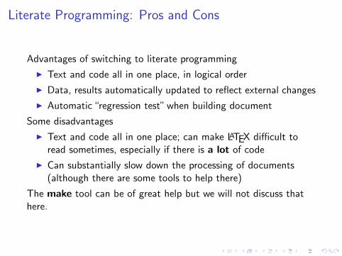
Literate Programming: Pros and Cons

Advantages of switching to literate programming

I Text and code all in one place, in logical order

I Data, results automatically updated to reflect external changes

I Automatic “regression test” when building document

Some disadvantages

I Text and code all in one place; can make LATEX difficult toread sometimes, especially if there is a lot of code

I Can substantially slow down the processing of documents(although there are some tools to help there)

The make tool can be of great help but we will not discuss thathere.

Sweave

What is Sweave?

I Sweave is a function and also a command-line script thatcomes with R (it is part of the utils package)

I The function can be invoked as Sweave()

I The command-line script is in the form R CMD Sweave

There is also Stangle

I Stangle()

I R CMD Stangle

But one thing at a time....

Basic Sweave Document: example.Rnw

\documentclass[11pt]{article}\title{My First Sweave Document}\begin{document}\maketitle

This is some text (i.e. a ``text chunk'').

Here is a code chunk<<>>=set.seed(1)x <- rnorm(100)mean(x)@\end{document}

Processing a Sweave Document

## create 'example.tex'## In Rlibrary(utils)Sweave("example.Rnw")

## On the command lineR CMD Sweave example.Rnw

## Usual LaTeX processing## One of the following will worktexi2dvi example.tex ## Create DVI filelatex example.textexi2dvi --pdf example.tex ## Create PDF filepdflatex example.tex

What R CMD Sweave Produces: example.tex

\documentclass[11pt]{article}\title{My First Sweave Document}\usepackage{Sweave}\begin{document}\maketitleThis is some text (i.e. a ``text chunk'').Here is a code chunk\begin{Schunk}\begin{Sinput}> set.seed(1)> x <- rnorm(100)> mean(x)\end{Sinput}\begin{Soutput}[1] 0.1088874\end{Soutput}\end{Schunk}\end{document}

The Resulting PDF Document

A Few Good Notes

Code chunks begin with

<<>>=

and end with

@

All R code goes in between.

Code chunks can have names, which is useful when we startmaking graphics (more later).

<<loaddata>>=## R code goes here@

By default, the code in a code chunk will be echoed, as will theresults of the computation (if there is something to print).

Note on Processing Sweave Documents

It’s important to remember that the order is

1. example.Rnw

2. example.tex

3. example.pdf

The .tex file is not something that we care about and should notedit (always edit the .Rnw file). It is merely an intermediarybetween the Sweave document and the PDF.

Basic Sweave Document: example2.Rnw

\documentclass[11pt]{article}\title{My First Sweave Document}\author{Roger D. Peng}\begin{document}\maketitle\section{Introduction}This is some text (i.e. a ``text chunk'').Here is a code chunk<<simulation,echo=false>>=set.seed(1)x <- rnorm(100)mean(x)@\end{document}

Result

Basic Sweave Document: example3.Rnw

\documentclass[11pt]{article}\title{My First Sweave Document}\begin{document}\maketitle

\section{Introduction}This is some text (i.e. a ``text chunk'').Here is a code chunk but it doesn't print anything!<<simulation,echo=false,results=hide>>=x <- rnorm(100); y <- x + rnorm(100, sd = 0.5)mean(x)@\end{document}

Result

Inline Text: example4.Rnw

\documentclass[11pt]{article}\begin{document}\section{Introduction}

<<computetime,echo=false>>=time <- format(Sys.time(), "%a %b %d %X %Y")rand <- rnorm(1)@The current time is \Sexpr{time}. My favorite randomnumber is \Sexpr{rand}.\end{document}

Inline Text

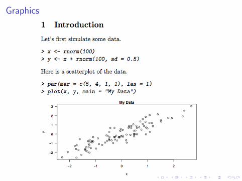
Graphics: example5.Rnw

\documentclass[11pt]{article}\begin{document}\section{Introduction}Let's first simulate some data.<<computetime,echo=true>>=x <- rnorm(100); y <- x + rnorm(100, sd = 0.5)@Here is a scatterplot of the data.<<scatterplot,fig=true,width=8,height=4>>=par(mar = c(5, 4, 1, 1), las = 1)plot(x, y, main = "My Data")@\end{document}

What Sweave Produces

\documentclass[11pt]{article}\usepackage{Sweave}

\begin{document}

\section{Introduction}Let's first simulate some data.\begin{Schunk}\begin{Sinput}> x <- rnorm(100)> y <- x + rnorm(100, sd = 0.5)\end{Sinput}\end{Schunk}

What Sweave Produces (cont’d)

Here is a scatterplot of the data.\begin{Schunk}\begin{Sinput}> par(mar = c(5, 4, 1, 1), las = 1)> plot(x, y, main = "My Data")\end{Sinput}\end{Schunk}

\includegraphics{example5-scatterplot}

\end{document}

Graphics

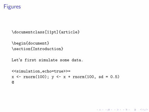
Figures

\documentclass[11pt]{article}

\begin{document}\section{Introduction}

Let's first simulate some data.

<<simulation,echo=true>>=x <- rnorm(100); y <- x + rnorm(100, sd = 0.5)@

Figures (cont’d)

Figure~\ref{plot} shows a scatterplot of the data.

\begin{figure}<<scatterplot,fig=true,width=8,height=4>>=par(mar = c(5, 4, 1, 1), las = 1)plot(x, y, main = "My Data")@\caption{Scatterplot}\label{plot}\end{figure}

\end{document}

Getting the Code Out

Sometimes it is easier to have all the R code in a separate file byitself, without all of the LATEX markup. We can use Stangle to dothat.

## In R> Stangle("example5.Rnw")Writing to file example5.R

## On the command lineamelia:> R CMD Stangle example5.RnwWriting to file example5.R

Then we can call source("example5.R") to run all the code inthe file.

Tangled Output

###################################################### chunk number 1: computetime###################################################x <- rnorm(100); y <- x + rnorm(100, sd = 0.5)

###################################################### chunk number 2: scatterplot###################################################par(mar = c(5, 4, 1, 1), las = 1)plot(x, y, main = "My Data")

Setting Global Options: example6.Rnw

Sometimes, we want to set options for every code chunk that arenon-default values. We can use \SweaveOpts to do that.

\SweaveOpts{option1=value1,option2=value2,...}

For example, we may want to suppress all code echoing and resultsoutput

\SweaveOpts{echo=false,results=hide}

The call to \SweaveOpts goes in the preamble.

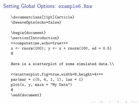
Setting Global Options: example6.Rnw

\documentclass[11pt]{article}\SweaveOpts{echo=false}

\begin{document}\section{Introduction}<<computetime,echo=true>>=x <- rnorm(100); y <- x + rnorm(100, sd = 0.5)@

Here is a scatterplot of some simulated data.\\

<<scatterplot,fig=true,width=8,height=4>>=par(mar = c(5, 4, 1, 1), las = 1)plot(x, y, main = "My Data")@\end{document}

Setting Global Options

Making Tables with xtable: example7.Rnw

\documentclass[11pt]{article}\begin{document}\section{Introduction}<<fitmodel>>=library(datasets)data(airquality)fit <- lm(Ozone ~ Wind + Temp + Solar.R, data = airquality)@

Here is a table of regression coefficients.\\

<<xtable,results=tex>>=library(xtable)xt <- xtable(summary(fit))print(xt)@\end{document}

Tables

Summary of Options

Output

I results: verbatim (default), tex, hide

I echo: true (default), false

I eval: true (default), false

Figures

I fig: true, false (default)

I width: width of plot (passed to plot device)

I height: height of plot (passed to plot device)

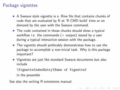
Package vignettes

I A Sweave style vignette is a .Rnw file that contains chunks ofcode that are evaluated by R at ’R CMD build’ time or ondemand by the user with the Sweave command.

I The code contained in those chunks should show a typicalworkflow i.e. the commands (+ output) issued by a userduring a typical interactive session with the package.

I The vignette should preferably demonstrates how to use thepackage to accomplish a non-trivial task. Why is this packageimportant?

I Vignettes are just like standard Sweave documents but alsoinclude

\VignetteIndexEntry{Name of Vignette}

in the preamble

See also the writing R extensions manual.

Package Directory Structure

Vignettes go in the inst/doc directory of the package

amelia:> ls./ .git/ NAMESPACE inst/ src/../ DESCRIPTION R/ man/ tests/amelia:> ls inst/doc./ Sweave.sty combined.bib filehash.pdf../ asa.bst filehash.Rnw

R CMD build will automatically try to build the vignette for you.

Finding Vignettes in R

> vignette()

Vignettes in package 'Matrix':

Comparisons Comparisons of Least Squares calculation speeds(source, pdf)

Design-issues Design Issues in Matrix package Development(source, pdf)

Intro2Matrix 2nd Introduction to the Matrix Package (source,pdf)

Introduction Introduction to the Matrix Package (source,pdf)

sparseModels Sparse Model Matrices (source, pdf)

Viewing Vignettes in R

## Launch vignette in (default) PDF viewervignette("filehash")

## Look at code in default text editorv <- vignette("filehash")edit(v)

Caching Computations

The cacheSweave package (on CRAN) can be used to cachelong-running computations when developing a Sweave document

<<longcomputation,cache=true>>==## Run MCMC samplerresult <- runmcmc(N = 10000)@

<<traceplot,fig=true>>=## Make trace plot of the parameter valuesplot(result)@

Processing Documents with cacheSweave

## In Rlibrary(cacheSweave)

## Set cache directory (default is ".")setCacheDir("cache")

## Process documentSweave("mydocument.Rnw", driver = cacheSweaveDriver)

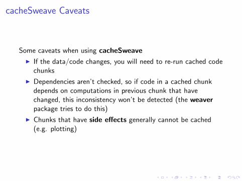
cacheSweave Caveats

Some caveats when using cacheSweave

I If the data/code changes, you will need to re-run cached codechunks

I Dependencies aren’t checked, so if code in a cached chunkdepends on computations in previous chunk that havechanged, this inconsistency won’t be detected (the weaverpackage tries to do this)

I Chunks that have side effects generally cannot be cached(e.g. plotting)

Reproducible Research Pipeline (Modified)

ComputationalResults

MeasuredData

AnalyticTables

Figures

Presentation code

Analytic codeProcessing code

Article

TextNumericalResults

Data

Reader

Author

Database