tutorial: topology optimization and result comparison

1

Tutorial: Topology Optimization and Result Comparison

(Made with Altair Inspire)

(Updated by Nimisha Srivastava)

2

SolidThinking Inspire Basics

The steps for running any optimization run in Altair Inspire are as follows:

1. Draw/Import Geometry:

The first step to start an optimization run is to draw or import the geometry which needs

to be optimized to obtain the final design.

• Drawing the geometry:

On clicking the geometry tab, a ribbon with various tool icons which can be used for creating

and editing the basic geometry within the tool.

Figure 1 Geometry Tools

• Importing the geometry:

If the basic geometry to be optimized and redesigned is already available, then it can be

imported into the tool directly using the File > Import option.

Altair Inspire supports most commercially available CAD formats.

Figure 2 Importing a File

3

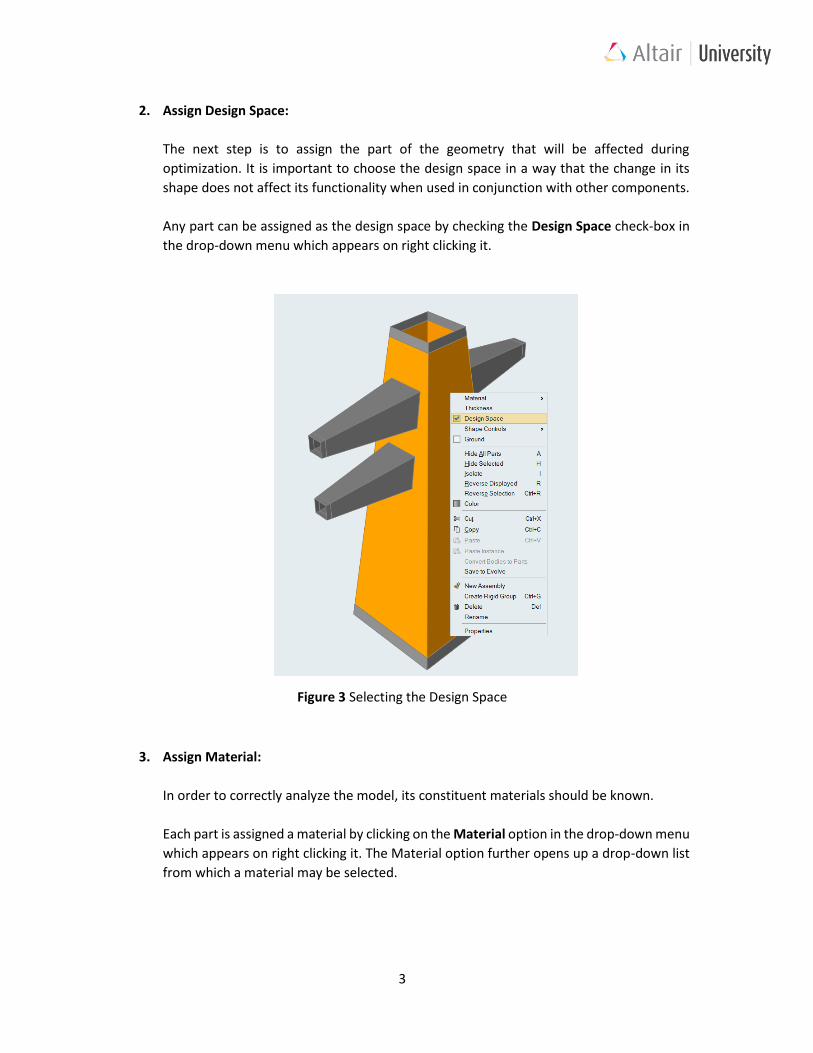
2. Assign Design Space:

The next step is to assign the part of the geometry that will be affected during

optimization. It is important to choose the design space in a way that the change in its

shape does not affect its functionality when used in conjunction with other components.

Any part can be assigned as the design space by checking the Design Space check-box in

the drop-down menu which appears on right clicking it.

Figure 3 Selecting the Design Space

3. Assign Material:

In order to correctly analyze the model, its constituent materials should be known.

Each part is assigned a material by clicking on the Material option in the drop-down menu

which appears on right clicking it. The Material option further opens up a drop-down list

from which a material may be selected.

4

Figure 4 Assigning Material

4. Defining the problem:

The physical problem may be defined by applying forces and fixing supports in accordance

to the given conditions using the Structure tab. Again, a ribbon with various tools which

may be used for setting up the physical problem appears.

Figure 5 Problem Set-up Tools

5. Run Optimization:

Click on the play button to run the optimization.

Figure 6 Run Optimization

Multi-sensitive icon for assigning supports and loads

5

Let’s try it! Tutorial: Topography Optimization

1. Opening the model:

• First, ensure that the MKS (m kg N s) unit system is activated by entering the File >

Preferences > Units to ‘m Kg N s’.

Figure 7 Setting the unit System

• Alternatively, use the dialogue at the bottom right hand corner

Figure 8 Tab for Changing Units

Tab for changing units

6

• Download the .stmod file provided with the tutorial and then open

topography_11_18.stmod it using the File> Open option.

Figure 9 Opening the .stmod file

• Once the file is opened, the interface should look something like this:

Figure 10 Interface after opening the file

7

2. Assigning the design space:

• Next, the design space is assigned. Right click on each of the parts and check the

Design Space check box.

Figure 11 Assigning the Design Space

• Alternatively, you may use the Model Browser and right click on the names of the

parts to be assigned as the design space and check the corresponding box in the drop-

down menu which appears.

Figure 12 Assigning the Design Space using Model Browser

8

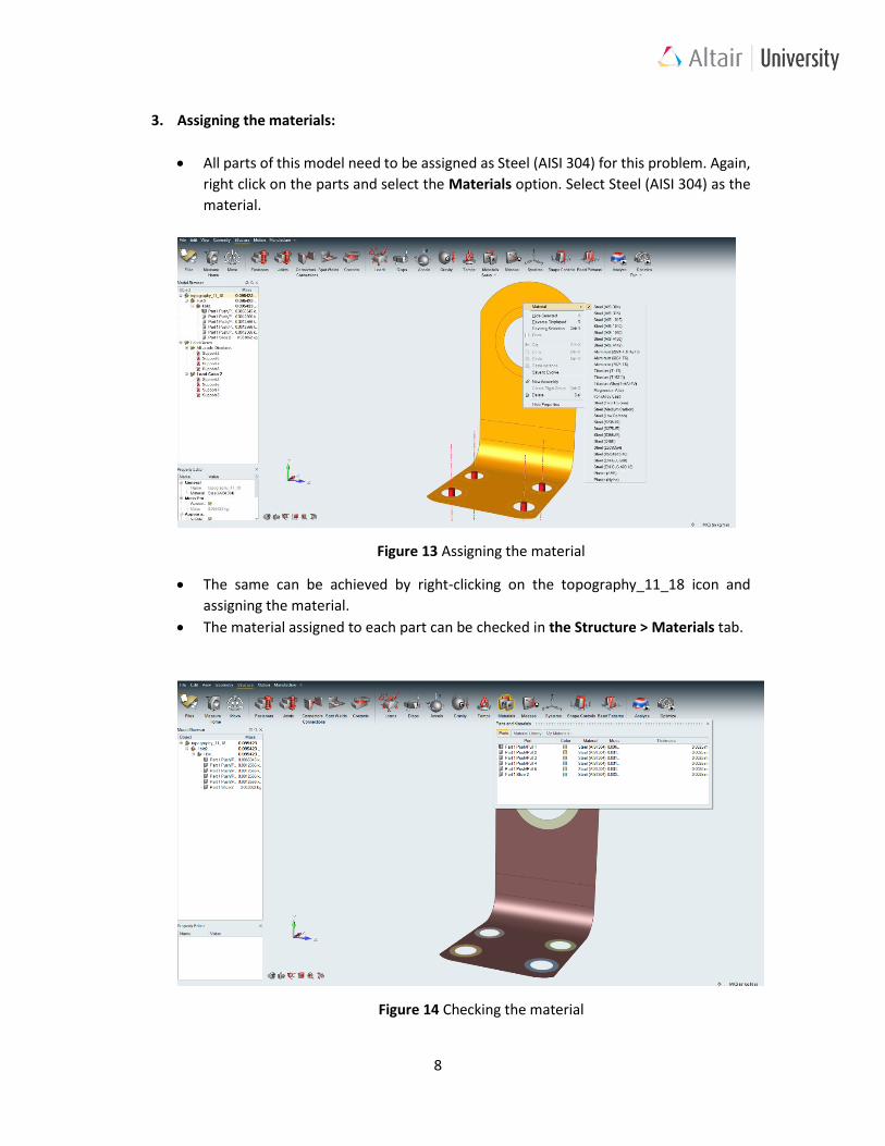
3. Assigning the materials:

• All parts of this model need to be assigned as Steel (AISI 304) for this problem. Again,

right click on the parts and select the Materials option. Select Steel (AISI 304) as the

material.

Figure 13 Assigning the material

• The same can be achieved by right-clicking on the topography_11_18 icon and

assigning the material.

• The material assigned to each part can be checked in the Structure > Materials tab.

Figure 14 Checking the material

9

4. Defining the Problem:

• First, select the parts from the Model Browser Review the thickness assigned to it. The

thickness of each part should be 2.5mm

• Next, we apply the constraints by using supports. Go to Structure > Loads and click on the

red cones on the multi sensitive icon to select apply supports.

Figure 15 Selecting apply supports in the Loads icon

• Click on one of the holes at the flat surface of the model. An orange support appears.

Repeat the process for all four holes. These supports will ensure that the bracket

remains grounded and that no lateral motion is allowed.

Figure 16 Supports at the bottom end

• Next, we will apply the loads by applying force on the connections created earlier. Go to

Structure > Loads and click on the red arrow to create a directional force.

10

Figure 17 Selecting apply force using the Loads icon

• Click on the Part 1 Push/Pull 1, as shown in the figure and apply a force of 50 N in the +x

direction.

Figure 18 Applying force

• Select Masses located in the Ribbon in Structure Tab and click on the center of the big

circular hole to place a concentrated mass.

Figure 19 Concentrated Masses Icon

• Enter 0.5 kg as the mass value.

11

• Click on the connect concentrated mass

Figure 20 Micro-dialog for a Concentrated Mass Created

• And select the inner edges of the circular hole displayed

Figure 21 Connecting the Concentrated Mass

• Since our objective is to obtain a symmetric design for the tower post optimization, we

will also add some shape control constraints by clicking on Structure > Shape Controls >

Symmetric.

• On selecting each of the designated Design Space, three dividing planes will appear in red.

The user can deactivate the undesired plane of symmetry by simply clicking on it.

• Deactivate the XZ and XY planes of symmetry, so that there’s only a symmetry along the

X axis. Now, optimization can be run.

12

Figure 22 The active planes of symmetry

13

5. Run Optimization

• After the set-up is complete, click on the play button on the Optimization icon.

• Select Topography as a Run Type

• Set the Minimum width to 15mm and let the Draw angle to 75 deg and maximum depth

to 5mm.

• Select Maximize frequencies and verify Load Case 2 is selected.

• Rename the run to topography_11_18_15mm.

• Click on Run

Figure 23 Run Settings for 15mm bead

• Repeat the runs for minimum width 10mm and 5mm as well, rename each run to reflect

the minimum bead width for clarity.

14

.

Figure 24 Optimized Models

Original Design Minimum bead width 15 mm

Minimum bead width 10 mm


15

6. Analysis

a. Analyzing the original design

• Click on the play button on the analyze icon.

Figure 25 The Analyze Icon

• Let the element size be 1 mm.

• Expand the normal Modes and select 10.

• Select Load Case 2 for the Use of supports from Load case.

• Select Faster for Speed/Accuracy.

• Select Sliding Only for the Contacts.

• Click run.

Figure 26 Settings for the Analysis

16

b. Analyzing the optimized designs

• Once an optimization is completed, the user can access each optimized model by

clicking on the optimize icon.

• A dialog box appears upon clicking the optimize icon, a dialog appears summarizing each

of the optimized models.

• Analysis can be conducted for each model by clicking on the Analyze button.

• Analyze each of the three models.

Figure 27 Shape Explorer

• Once the analysis runs are complete, each of them can be accessed by clicking on the

analyze button.

Figure 28 Click here for the analysis results

17

7. Results

• First view the results for each of the runs, view the displacement results and compare

them for each of the cases.

Figure 29 Displacement Contours for all Models




Original Design

18

• Although the contour graphs for each of the models are pretty similar, owing the similar

problem set-up, the values of the maximum displacement are widely removed from each

other.

As the minimum bead width decreases, the value of the maximum displacement drops

considerably as indicated by the following table.

Model Maximum Displacement (mm)

Original Design 0.6389

Minimum bead width - 15 mm 0.4825

Minimum bead width - 10 mm 0.3424

Minimum bead width - 5mm 0.1595

• Access this information from the compare button on the lower right corner on the dialog

which appears upon clicking the Analyze button.

Figure 30 Compare Results Button

• Toggle between the various result types to compare different quantities such as Von-

Mises Stress.

Compare Results Button

19

Figure 31 Von Mises Stress Distribution

• The values for the maximum and minimum values of Von Mises stress can again be

accessed by using the Compare Results button.




Original Design

20

Model Maximum Von Mises Stress

Original Design 10.840 × 107 Pa

Minimum bead width - 15 mm 9.235 × 107 Pa



• Finally, the frequencies of the normal modes for each of the models can be accessed by

looking at the Normal Modes load case.

Figure 32 Viewing Modal Frequencies

• The frequency of the first mode has been summarized for each of the models below.

Model First Mode Frequency

Original Design 2.927 × 102

Minimum bead width - 15 mm 3.368 × 102



Select Normal Modes for

viewing the mode

frequencies

tutorial: topology optimization and result comparison

Documents