tutorial - using arcgis 3d analyst
TRANSCRIPT
ArcGIS®
9Using ArcGIS® 3D Analyst™
Copyright © 2000–2004 ESRIAll rights reserved.Printed in the United States of America.
The information contained in this document is the exclusive property of ESRI. This work is protected under United States copyright law and otherinternational copyright treaties and conventions. No part of this work may be reproduced or transmitted in any form or by any means, electronic ormechanical, including photocopying and recording, or by any information storage or retrieval system, except as expressly permitted in writing by ESRI. Allrequests should be sent to Attention: Contracts Manager, ESRI, 380 New York Street, Redlands, CA 92373-8100, USA.
The information contained in this document is subject to change without notice.
DATA CREDITSExercise 1: Death Valley image data courtesy of National Aeronautics and Space Administration (NASA)/Jet Propulsion Laboratory (JPL)/Caltech.
Exercise 2: San Gabriel Basin data courtesy of the San Gabriel Basin Water Quality Authority.
Exercise 3: Belarus CS137 soil contamination and thyroid cancer data courtesy of the International Sakharov Environmental University.
Exercise 4: Hidden River Cave data courtesy of the American Cave Conservation Association.
Exercise 5: Elevation and image data courtesy of MassGIS, Commonwealth of Massachusetts Executive Office of Environmental Affairs.Exercise 6: Las Vegas Millennium Mosaic (Year 2000 Landsat) and QuickBird images data courtesy of DigitalGlobe.Exercise 7: Ozone concentration raster derived from data courtesy of the California Air Resources Board, Southern California Millennium Mosaic (Year2000 Landsat) image courtesy of DigitalGlobe, Angelus Oaks imagery courtesy of AirPhoto USA, Southwestern U.S. elevation data derived from U.S.
National Elevation Data courtesy of the U.S. Geological Survey.
CONTRIBUTING WRITERSSteve Bratt, Bob Booth
U.S. GOVERNMENT RESTRICTED/LIMITED RIGHTSAny software, documentation, and/or data delivered hereunder is subject to the terms of the License Agreement. In no event shall the U.S. Government
acquire greater than RESTRICTED/LIMITED RIGHTS. At a minimum, use, duplication, or disclosure by the U.S. Government is subject to restrictions as
set forth in FAR §52.227-14 Alternates I, II, and III (JUN 1987); FAR §52.227-19 (JUN 1987) and/or FAR §12.211/12.212 (Commercial Technical Data/
Computer Software); and DFARS §252.227-7015 (NOV 1995) (Technical Data) and/or DFARS §227.7202 (Computer Software), as applicable. Contractor/
Manufacturer is ESRI, 380 New York Street, Redlands, CA 92373-8100, USA.
ESRI, the ESRI globe logo, 3D Analyst, ArcInfo, ArcCatalog, ArcMap, ArcScene, ArcGIS, GIS by ESRI, ArcGlobe, ArcEditor, ArcView, the ArcGIS logo, and
www.esri.com are trademarks, registered trademarks, or service marks of ESRI in the United States, the European Community, or certain other
jurisdictions.
Portions of this software are under license from GeoFusion, Inc. Copyright © 2002, GeoFusion, Inc. All rights reserved.
Other companies and products mentioned herein are trademarks or registered trademarks of their respective trademark owners.
IN THIS CHAPTER
9
Quick-start tutorial 2• Copying the tutorial data
• Exercise 1: Draping an image overa terrain surface
• Exercise 2: Visualizingcontamination in an aquifer
• Exercise 3: Visualizing soilcontamination and thyroid cancerrates
• Exercise 4: Building a TIN torepresent terrain
• Exercise 5: Working withanimations in ArcScene
• Exercise 6: ArcGlobe basics
• Exercise 7: ArcGlobe layer classification
The best way to learn 3D Analyst is to use it. In the exercises in thistutorial, you will:
• Use ArcCatalog to find and preview 3D data.
• Add data to ArcScene.
• Set 3D properties for viewing data.
• Create new 3D feature data from 2D features and surfaces.
• Create new raster surface data from point data.
• Build a TIN surface from existing feature data.
• Make animations.
• Learn how to use ArcGlobe and manage its data content.
In order to use this tutorial, you need to have the 3D Analyst extensionand ArcGIS installed and have the tutorial data installed on a local orshared network drive on your system. Ask your system administrator forthe correct path to the tutorial data if you do not find it at the defaultinstallation path specified in the tutorial.
10 USING ARCGIS 3D ANALYST
Copying the tutorial data
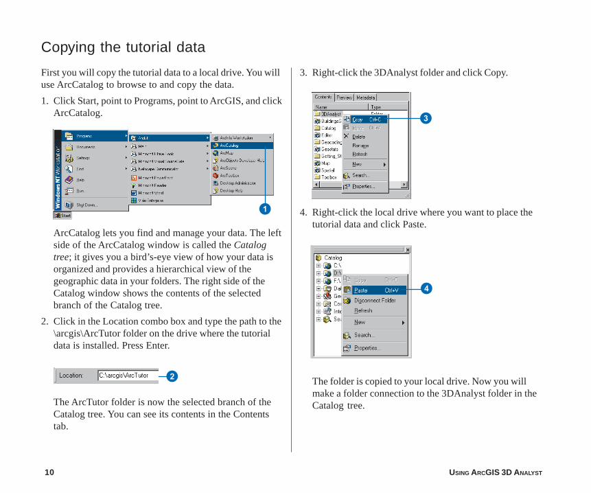
First you will copy the tutorial data to a local drive. You willuse ArcCatalog to browse to and copy the data.
1. Click Start, point to Programs, point to ArcGIS, and clickArcCatalog.
3. Right-click the 3DAnalyst folder and click Copy.
1
ArcCatalog lets you find and manage your data. The leftside of the ArcCatalog window is called the Catalogtree; it gives you a bird’s-eye view of how your data isorganized and provides a hierarchical view of thegeographic data in your folders. The right side of theCatalog window shows the contents of the selectedbranch of the Catalog tree.
2. Click in the Location combo box and type the path to the\arcgis\ArcTutor folder on the drive where the tutorialdata is installed. Press Enter.
The ArcTutor folder is now the selected branch of theCatalog tree. You can see its contents in the Contentstab.
4. Right-click the local drive where you want to place thetutorial data and click Paste.
The folder is copied to your local drive. Now you willmake a folder connection to the 3DAnalyst folder in theCatalog tree.
4
2
3
QUICK-START TUTORIAL 11
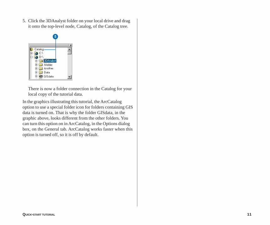
5. Click the 3DAnalyst folder on your local drive and dragit onto the top-level node, Catalog, of the Catalog tree.
There is now a folder connection in the Catalog for yourlocal copy of the tutorial data.
In the graphics illustrating this tutorial, the ArcCatalogoption to use a special folder icon for folders containing GISdata is turned on. That is why the folder GISdata, in thegraphic above, looks different from the other folders. Youcan turn this option on in ArcCatalog, in the Options dialogbox, on the General tab. ArcCatalog works faster when thisoption is turned off, so it is off by default.
5
12 USING ARCGIS 3D ANALYST
Viewing a remotely sensed image draped over a terrainsurface can often lead to greater understanding of thepatterns in the image and how they relate to the shape ofthe earth’s surface.
Imagine that you’re a geologist studying Death Valley,California. You have collected a TIN that shows the terrainand a satellite radar image that shows the roughness of theland surface. The image is highly informative, but you canadd a dimension to your understanding by draping the imageover the terrain surface. Death Valley image data wassupplied courtesy of NASA/JPL/Caltech.
Turning on the 3D Analyst extension
You will need to enable the 3D Analyst extension.
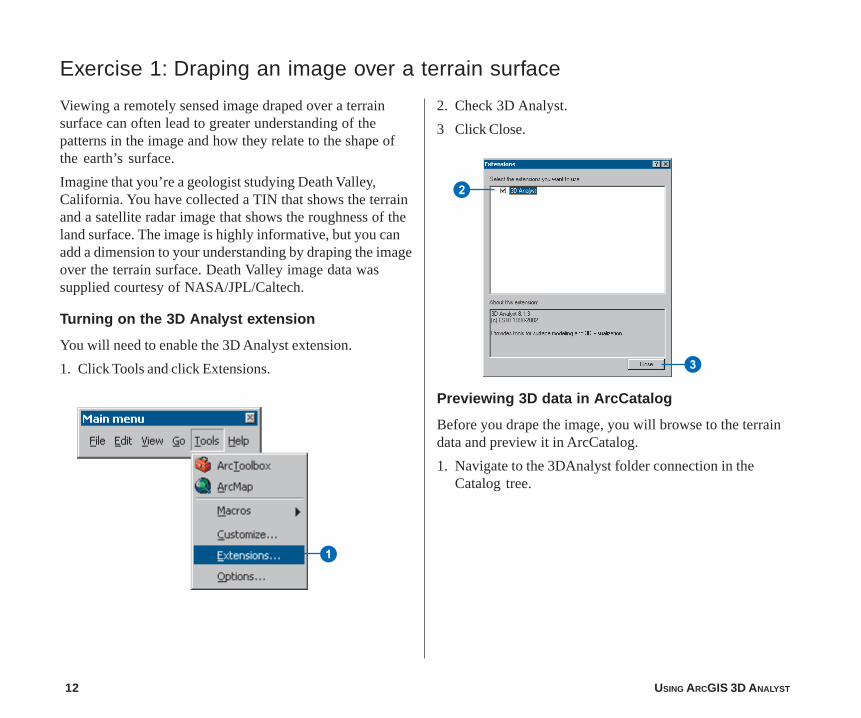
1. Click Tools and click Extensions.
Exercise 1: Draping an image over a terrain surface
2. Check 3D Analyst.
3 Click Close.
Previewing 3D data in ArcCatalog
Before you drape the image, you will browse to the terraindata and preview it in ArcCatalog.
1. Navigate to the 3DAnalyst folder connection in theCatalog tree.
1
2
3
QUICK-START TUTORIAL 13
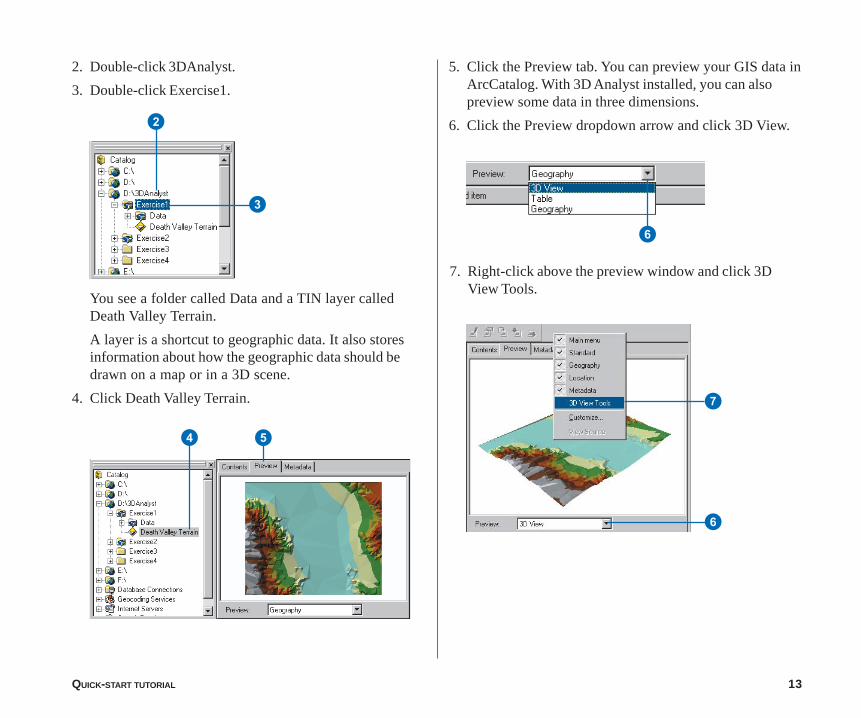
2. Double-click 3DAnalyst.
3. Double-click Exercise1.
5. Click the Preview tab. You can preview your GIS data inArcCatalog. With 3D Analyst installed, you can alsopreview some data in three dimensions.
6. Click the Preview dropdown arrow and click 3D View.
You see a folder called Data and a TIN layer calledDeath Valley Terrain.
A layer is a shortcut to geographic data. It also storesinformation about how the geographic data should bedrawn on a map or in a 3D scene.
4. Click Death Valley Terrain.
4 5
7. Right-click above the preview window and click 3DView Tools.
7
6
2
3
6
14 USING ARCGIS 3D ANALYST
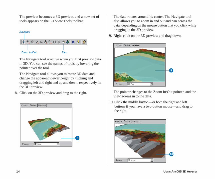
The preview becomes a 3D preview, and a new set oftools appears on the 3D View Tools toolbar.
The data rotates around its center. The Navigate toolalso allows you to zoom in and out and pan across thedata, depending on the mouse button that you click whiledragging in the 3D preview.
9. Right-click on the 3D preview and drag down.
8
The Navigate tool is active when you first preview datain 3D. You can see the names of tools by hovering thepointer over the tool.
The Navigate tool allows you to rotate 3D data andchange the apparent viewer height by clicking anddragging left and right and up and down, respectively, inthe 3D preview.
8. Click on the 3D preview and drag to the right. The pointer changes to the Zoom In/Out pointer, and theview zooms in to the data.
10. Click the middle button—or both the right and leftbuttons if you have a two-button mouse—and drag tothe right.
Q
9
Navigate
Zoom In/Out Pan

QUICK-START TUTORIAL 15
The pointer changes to the Pan pointer, and the viewpans across the data.
11. Click the Identify button and click on the TIN.
The view returns to the full extent of the data.
The Identify Results window shows you the elevation,slope, and aspect of the surface at the point you clicked.
12. Close the Identify Results window.
13. Click the Full Extent button.
Now you’ve examined the surface data and begun to learnhow to navigate in 3D. The next step is to start ArcSceneand add your radar image to a new scene.
Starting ArcScene and adding data
ArcScene is the 3D viewer for 3D Analyst. Although youcan preview 3D data in ArcCatalog, ArcScene allows youto build up complex scenes with multiple sources of data.
1. Click the ArcScene button on the 3D View Tools toolbar.R
E
Identify
ArcScene
16 USING ARCGIS 3D ANALYST
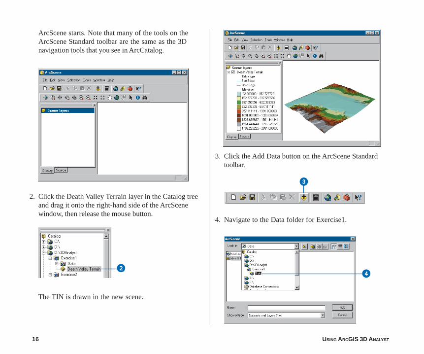
ArcScene starts. Note that many of the tools on theArcScene Standard toolbar are the same as the 3Dnavigation tools that you see in ArcCatalog.
3. Click the Add Data button on the ArcScene Standardtoolbar.
3
4. Navigate to the Data folder for Exercise1.
2. Click the Death Valley Terrain layer in the Catalog treeand drag it onto the right-hand side of the ArcScenewindow, then release the mouse button.
The TIN is drawn in the new scene.
42

QUICK-START TUTORIAL 17
5. Click dvim3.TIF.
6. Click Add.
7. Uncheck the Death Valley Terrain layer.
7
The image is added to the scene.
The image is drawn on a plane, with a base elevationvalue of zero. You can see it above the Death Valleyterrain surface where the terrain is below 0 meterselevation (sea level); it is hidden by the terrain surfaceeverywhere else.
Now you can see the whole image. The black areas areparts of the image that contain no data and are a resultof previous processing to fit the image to the terrain.
You have added the image to the scene. Now you willchange the properties of the image layer so that the imagewill be draped over the terrain surface.
Draping the image
While the surface texture information shown in the image isa great source of information about the terrain, somerelationships between the surface texture and the shape ofthe terrain will be apparent when you drape the image overthe terrain surface. In ArcScene, you can drape a layer—containing a grid, image, or 2D features—over a surface (agrid or TIN) by assigning the base heights of the layer fromthe surface.
5
6
18 USING ARCGIS 3D ANALYST
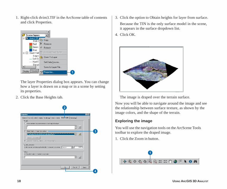
1. Right-click dvim3.TIF in the ArcScene table of contentsand click Properties.
3. Click the option to Obtain heights for layer from surface.
Because the TIN is the only surface model in the scene,it appears in the surface dropdown list.
4. Click OK.
1
1
The layer Properties dialog box appears. You can changehow a layer is drawn on a map or in a scene by settingits properties.
2. Click the Base Heights tab. The image is draped over the terrain surface.
Now you will be able to navigate around the image and seethe relationship between surface texture, as shown by theimage colors, and the shape of the terrain.
Exploring the image
You will use the navigation tools on the ArcScene Toolstoolbar to explore the draped image.
1. Click the Zoom in button.
2
3
4
QUICK-START TUTORIAL 19
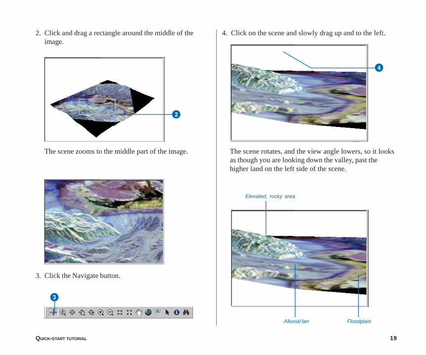
2. Click and drag a rectangle around the middle of theimage.
4. Click on the scene and slowly drag up and to the left.
2
3
4
The scene zooms to the middle part of the image.
3. Click the Navigate button.
The scene rotates, and the view angle lowers, so it looksas though you are looking down the valley, past thehigher land on the left side of the scene.
Elevated, rocky area
FloodplainAlluvial fan
20 USING ARCGIS 3D ANALYST
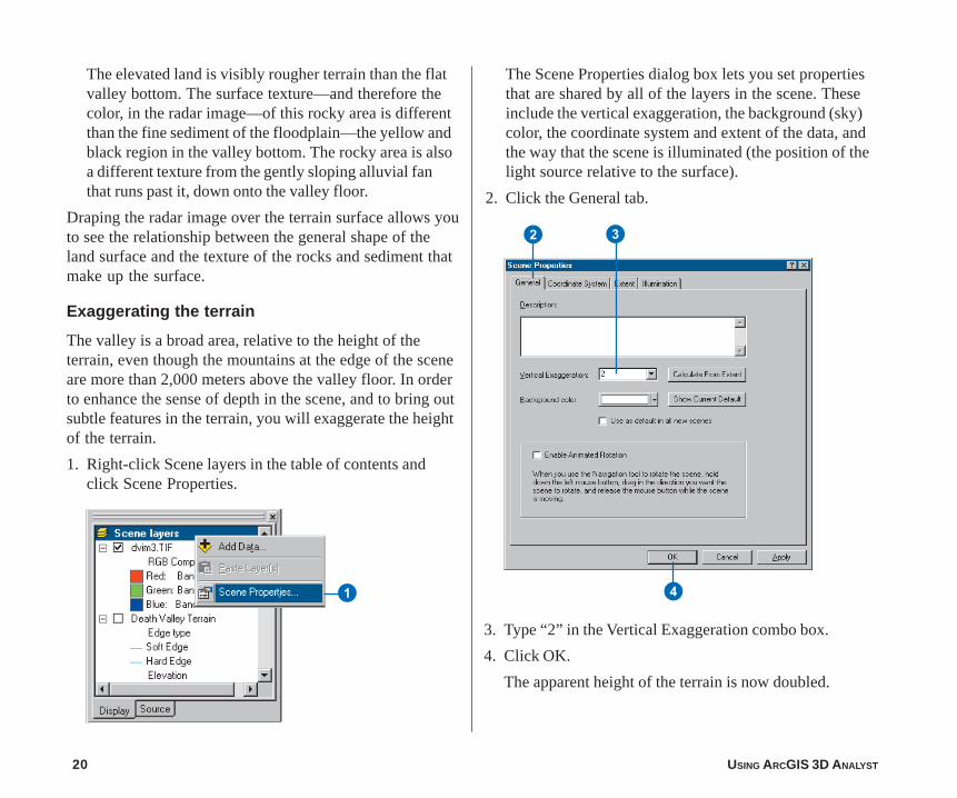
The Scene Properties dialog box lets you set propertiesthat are shared by all of the layers in the scene. Theseinclude the vertical exaggeration, the background (sky)color, the coordinate system and extent of the data, andthe way that the scene is illuminated (the position of thelight source relative to the surface).
2. Click the General tab.
2 3
4
3. Type “2” in the Vertical Exaggeration combo box.
4. Click OK.
The apparent height of the terrain is now doubled.
The elevated land is visibly rougher terrain than the flatvalley bottom. The surface texture—and therefore thecolor, in the radar image—of this rocky area is differentthan the fine sediment of the floodplain—the yellow andblack region in the valley bottom. The rocky area is alsoa different texture from the gently sloping alluvial fanthat runs past it, down onto the valley floor.
Draping the radar image over the terrain surface allows youto see the relationship between the general shape of theland surface and the texture of the rocks and sediment thatmake up the surface.
Exaggerating the terrain
The valley is a broad area, relative to the height of theterrain, even though the mountains at the edge of the sceneare more than 2,000 meters above the valley floor. In orderto enhance the sense of depth in the scene, and to bring outsubtle features in the terrain, you will exaggerate the heightof the terrain.
1. Right-click Scene layers in the table of contents andclick Scene Properties.
1
QUICK-START TUTORIAL 21
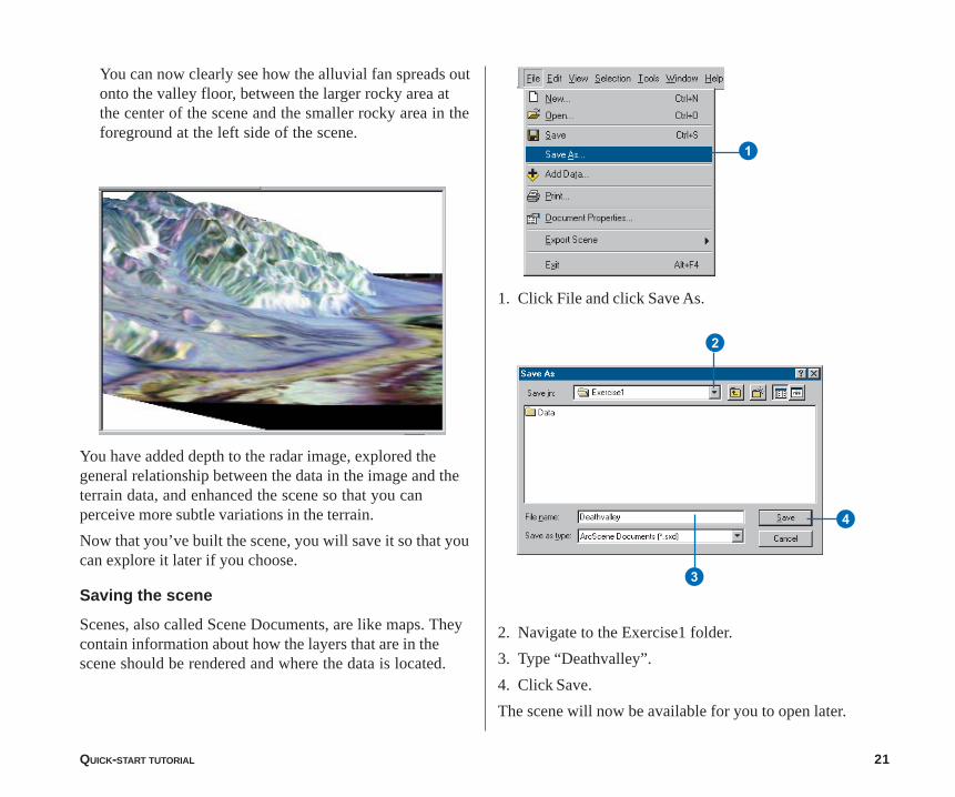
You can now clearly see how the alluvial fan spreads outonto the valley floor, between the larger rocky area atthe center of the scene and the smaller rocky area in theforeground at the left side of the scene.
1
1. Click File and click Save As.
You have added depth to the radar image, explored thegeneral relationship between the data in the image and theterrain data, and enhanced the scene so that you canperceive more subtle variations in the terrain.
Now that you’ve built the scene, you will save it so that youcan explore it later if you choose.
Saving the scene
Scenes, also called Scene Documents, are like maps. Theycontain information about how the layers that are in thescene should be rendered and where the data is located.
2. Navigate to the Exercise1 folder.
3. Type “Deathvalley”.
4. Click Save.
The scene will now be available for you to open later.
2
3
4

22 USING ARCGIS 3D ANALYST
Exercise 2: Visualizing contamination in an aquifer
Imagine that you work for a water district. The district isaware of some areas where volatile organic compounds(VOCs) have leaked over the years. Scientists from yourdepartment have mapped some plumes of VOCs in theaquifer, and you want to create a 3D scene to help officialsand the public visualize the extent of the problem.
Some of the data for the scene has already been assembledin the Groundwater scene. You will modify the scene tobetter communicate the problem.
VOC data was supplied courtesy of the San Gabriel BasinWater Quality Authority.
Opening the Groundwater scene document
This scene document contains a TIN that shows the shapeof the contaminant plume, a raster that shows theconcentration of the contaminant, and two shapefiles thatshow the locations of parcels and wells. You will drape theconcentration raster over the plume TIN, extrude thebuilding features and change their color, and extrude thewell features so that the wells that are most endangered bythe contamination may be more easily recognized.
1. In ArcScene, click File, then click Open.
3. Click Groundwater.sxd.
2. Navigate to the Exercise2 folder.
4. Click Open.
The Groundwater scene opens. You can see the fourlayers in the table of contents.
Showing the volume and intensity ofcontamination
You’ll drape the raster of VOC concentration over the TINof the contaminant plume surface to show the volume andintensity of contamination in the aquifer.
1. Right-click congrd and click Properties.
1
4
3
1
QUICK-START TUTORIAL 23
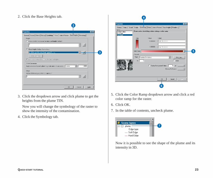
2. Click the Base Heights tab.
5. Click the Color Ramp dropdown arrow and click a redcolor ramp for the raster.
6. Click OK.
7. In the table of contents, uncheck plume.
2
3
4
5
6
3. Click the dropdown arrow and click plume to get theheights from the plume TIN.
Now you will change the symbology of the raster toshow the intensity of the contamination.
4. Click the Symbology tab.
Now it is possible to see the shape of the plume and itsintensity in 3D.
7
24 USING ARCGIS 3D ANALYST
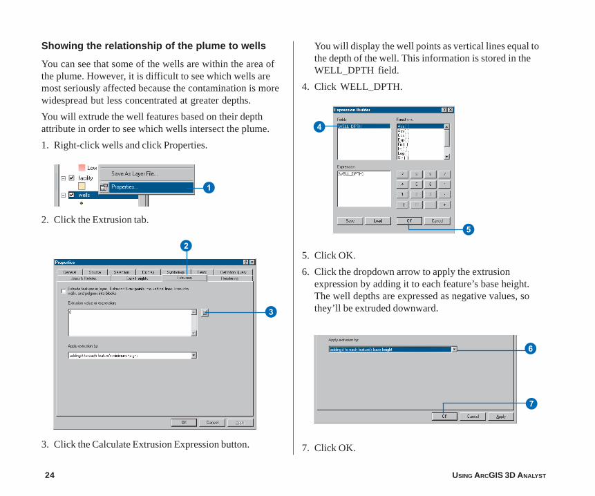
Showing the relationship of the plume to wells
You can see that some of the wells are within the area ofthe plume. However, it is difficult to see which wells aremost seriously affected because the contamination is morewidespread but less concentrated at greater depths.
You will extrude the well features based on their depthattribute in order to see which wells intersect the plume.
1. Right-click wells and click Properties.
You will display the well points as vertical lines equal tothe depth of the well. This information is stored in theWELL_DPTH field.
4. Click WELL_DPTH.
2. Click the Extrusion tab.
3. Click the Calculate Extrusion Expression button.
5. Click OK.
6. Click the dropdown arrow to apply the extrusionexpression by adding it to each feature’s base height.The well depths are expressed as negative values, sothey’ll be extruded downward.
7. Click OK.
1
3
2
4
5
6
7

QUICK-START TUTORIAL 25
You can see the places where the wells intersect, or areclose to, the plume. Now you will modify the scene to showthe priority of various facilities that have been targeted forcleanup.
Showing the facilities with a high cleanup priority
Analysts in your department have ranked the facilitiesaccording to the urgency of a cleanup at each location.You’ll extrude the facilities into 3D columns and color codethem to emphasize those with a higher priority for cleanup.
1. Right-click facility and click Properties.
2. Click the Extrusion tab.
5. Type “* 100”.
3. Click the Calculate Extrusion Expression button.
4. Click PRIORITY1.
6. Click OK.
The expression you created appears in the Extrusionvalue or expression box.
3
2
4
6
26 USING ARCGIS 3D ANALYST
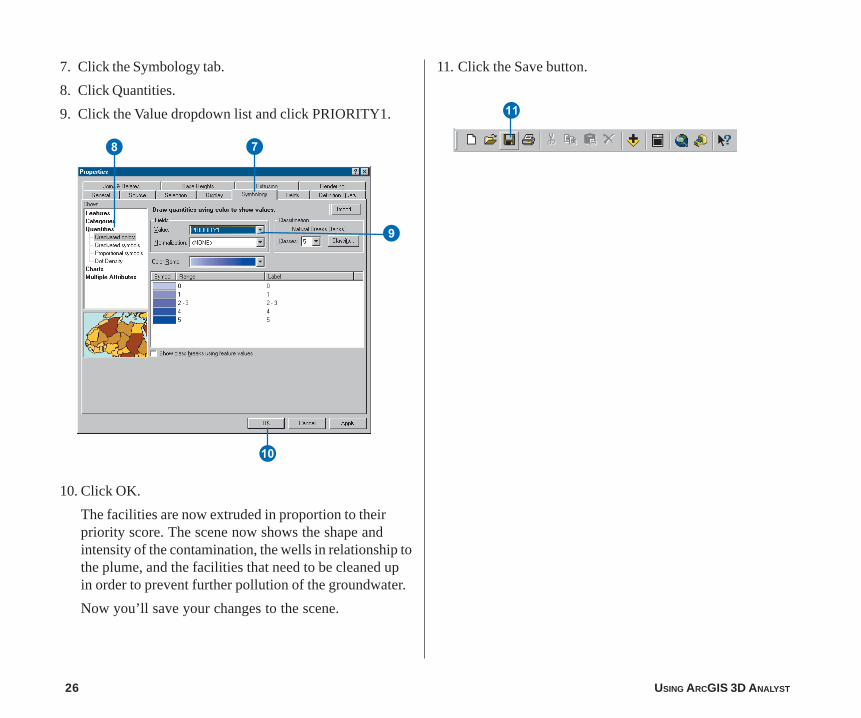
7. Click the Symbology tab.
8. Click Quantities.
9. Click the Value dropdown list and click PRIORITY1.
78
9
Q
11. Click the Save button.
10. Click OK.
The facilities are now extruded in proportion to theirpriority score. The scene now shows the shape andintensity of the contamination, the wells in relationship tothe plume, and the facilities that need to be cleaned upin order to prevent further pollution of the groundwater.
Now you’ll save your changes to the scene.
W
QUICK-START TUTORIAL 27
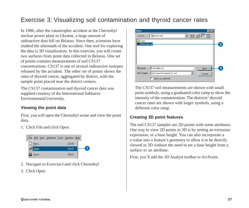
Exercise 3: Visualizing soil contamination and thyroid cancer rates
In 1986, after the catastrophic accident at the Chernobylnuclear power plant in Ukraine, a large amount ofradioactive dust fell on Belarus. Since then, scientists havestudied the aftermath of the accident. One tool for exploringthe data is 3D visualization. In this exercise, you will createtwo surfaces from point data collected in Belarus. One setof points contains measurements of soil CS137concentrations. CS137 is one of several radioactive isotopesreleased by the accident. The other set of points shows therates of thyroid cancer, aggregated by district, with thesample point placed near the district centers.
The CS137 contamination and thyroid cancer data wassupplied courtesy of the International SakharovEnvironmental University.
Viewing the point data
First, you will open the Chernobyl scene and view the pointdata.
1. Click File and click Open.
The CS137 soil measurements are shown with smallpoint symbols, using a graduated color ramp to show theintensity of the contamination. The districts’ thyroidcancer rates are shown with larger symbols, using adifferent color ramp.
Creating 3D point features
The soil CS137 samples are 2D points with some attributes.One way to view 2D points in 3D is by setting an extrusionexpression, or a base height. You can also incorporate az-value into a feature’s geometry to allow it to be directlyviewed in 3D without the need to set a base height from asurface or an attribute.
First, you’ll add the 3D Analyst toolbar to ArcScene.
2. Navigate to Exercise3 and click Chernobyl.
3. Click Open.
1
2
3
28 USING ARCGIS 3D ANALYST
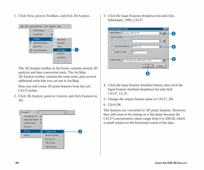
1. Click View, point to Toolbars, and click 3D Analyst. 3. Click the Input Features dropdown list and clickSubsample_1994_CS137.
The 3D Analyst toolbar in ArcScene contains several 3Danalysis and data conversion tools. The ArcMap3D Analyst toolbar contains the same tools, plus severaladditional tools that you can use in ArcMap.
Now you will create 3D point features from the soilCS137 points.
2. Click 3D Analyst, point to Convert, and click Features to3D.
4. Click the Input Feature Attribute button, then click theInput Feature Attribute dropdown list and clickCS137_CI_K.
5. Change the output feature name to CS137_3D.
6. Click OK.
The features are converted to 3D point features. However,they still seem to be resting on a flat plane because theCS137 concentration values range from 0 to 208.68, whichis small relative to the horizontal extent of the data.
1
2
3
4
5
6
QUICK-START TUTORIAL 29
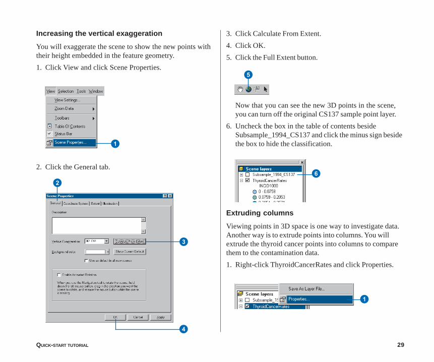
Increasing the vertical exaggeration
You will exaggerate the scene to show the new points withtheir height embedded in the feature geometry.
1. Click View and click Scene Properties.
3. Click Calculate From Extent.
4. Click OK.
5. Click the Full Extent button.
5
2. Click the General tab.
Now that you can see the new 3D points in the scene,you can turn off the original CS137 sample point layer.
6. Uncheck the box in the table of contents besideSubsample_1994_CS137 and click the minus sign besidethe box to hide the classification.
Extruding columns
Viewing points in 3D space is one way to investigate data.Another way is to extrude points into columns. You willextrude the thyroid cancer points into columns to comparethem to the contamination data.
1. Right-click ThyroidCancerRates and click Properties.
1
2
3
4
6
1
30 USING ARCGIS 3D ANALYST
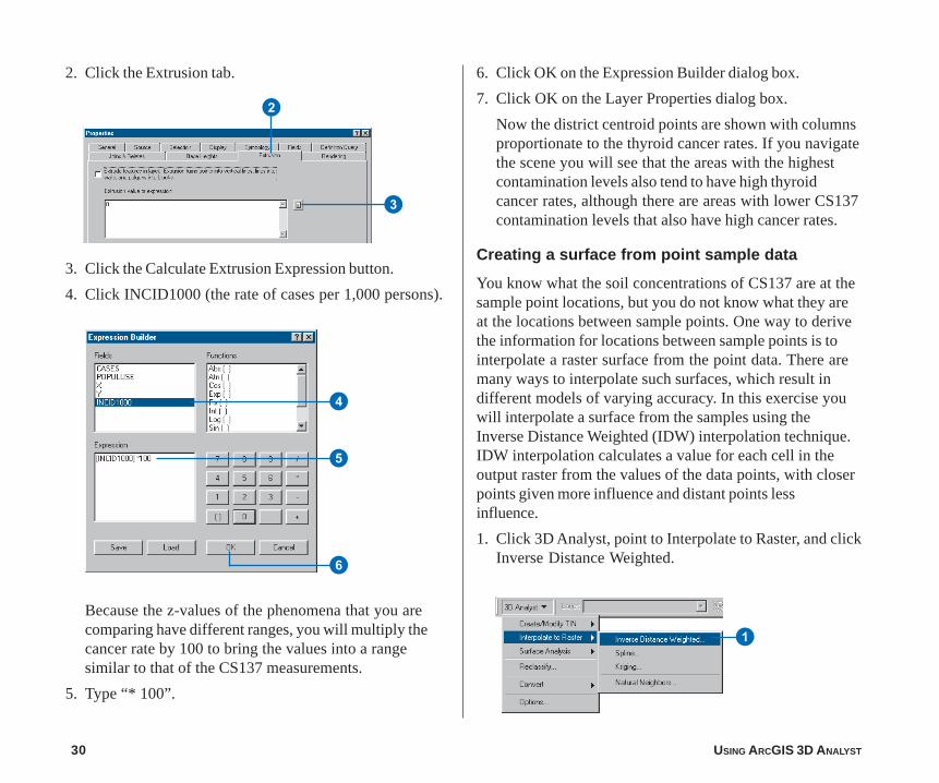
2. Click the Extrusion tab. 6. Click OK on the Expression Builder dialog box.
7. Click OK on the Layer Properties dialog box.
Now the district centroid points are shown with columnsproportionate to the thyroid cancer rates. If you navigatethe scene you will see that the areas with the highestcontamination levels also tend to have high thyroidcancer rates, although there are areas with lower CS137contamination levels that also have high cancer rates.
Creating a surface from point sample data
You know what the soil concentrations of CS137 are at thesample point locations, but you do not know what they areat the locations between sample points. One way to derivethe information for locations between sample points is tointerpolate a raster surface from the point data. There aremany ways to interpolate such surfaces, which result indifferent models of varying accuracy. In this exercise youwill interpolate a surface from the samples using theInverse Distance Weighted (IDW) interpolation technique.IDW interpolation calculates a value for each cell in theoutput raster from the values of the data points, with closerpoints given more influence and distant points lessinfluence.
1. Click 3D Analyst, point to Interpolate to Raster, and clickInverse Distance Weighted.
3. Click the Calculate Extrusion Expression button.
4. Click INCID1000 (the rate of cases per 1,000 persons).
Because the z-values of the phenomena that you arecomparing have different ranges, you will multiply thecancer rate by 100 to bring the values into a rangesimilar to that of the CS137 measurements.
5. Type “* 100”.
1
4
6
5
2
3

QUICK-START TUTORIAL 31
2. Click the Input points dropdown list and clickSubsample_1994_CS137.
6. Click Save.
7. Click OK.
3. Click the Z value field dropdown list and clickCS137_CI_K.
4. Click the Browse button.
5. Navigate to the Exercise3 folder and type“CS137_IDW” in the Name field.
ArcScene interpolates the surface and adds it to the scene.
2
3
4
5
6
7
32 USING ARCGIS 3D ANALYST
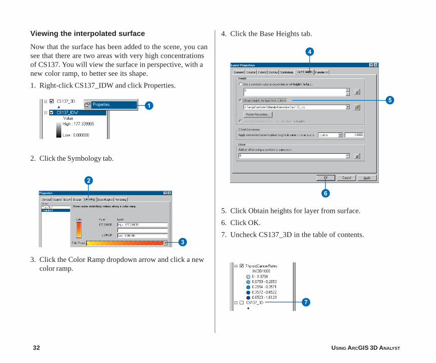
Viewing the interpolated surface
Now that the surface has been added to the scene, you cansee that there are two areas with very high concentrationsof CS137. You will view the surface in perspective, with anew color ramp, to better see its shape.
1. Right-click CS137_IDW and click Properties.
4. Click the Base Heights tab.
1
2. Click the Symbology tab.
3. Click the Color Ramp dropdown arrow and click a newcolor ramp.
5. Click Obtain heights for layer from surface.
6. Click OK.
7. Uncheck CS137_3D in the table of contents.
2
3
7
4
5
6

QUICK-START TUTORIAL 33
Now you can see the interpolated surface of CS137contamination, along with the thyroid cancer rate data.
3. Double-click INCID1000 in the Fields list.
Next, you will select the province centers with thehighest rates of thyroid cancer.
Selecting features by an attribute
Sometimes it is important to focus on a specific set of dataor specific features. You can select features in a scene bytheir location, by their attributes, or by clicking them withthe Select Features tool. You will select the provincecenters by attribute to find the locations with the highestrates.
1. Click Selection and click Select By Attributes.
2. Click the Layer dropdown arrow and clickThyroidCancerRates.
1
2
3
34 USING ARCGIS 3D ANALYST
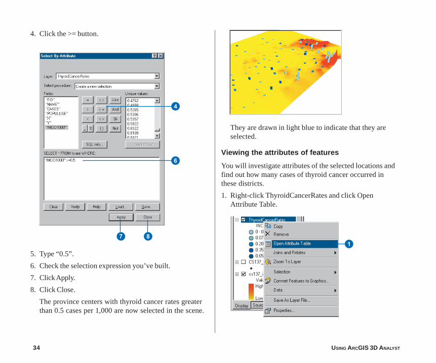
4. Click the >= button.
They are drawn in light blue to indicate that they areselected.
Viewing the attributes of features
You will investigate attributes of the selected locations andfind out how many cases of thyroid cancer occurred inthese districts.
1. Right-click ThyroidCancerRates and click OpenAttribute Table.
5. Type “0.5”.
6. Check the selection expression you’ve built.
7. Click Apply.
8. Click Close.
The province centers with thyroid cancer rates greaterthan 0.5 cases per 1,000 are now selected in the scene.
4
6
7 81
QUICK-START TUTORIAL 35
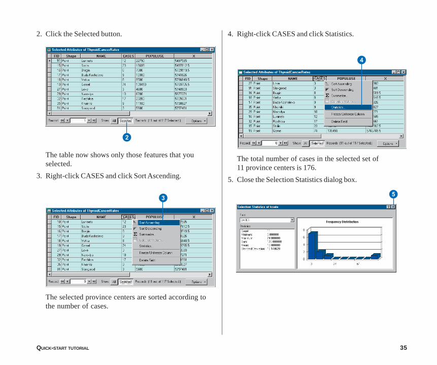
2. Click the Selected button. 4. Right-click CASES and click Statistics.
4
The table now shows only those features that youselected.
3. Right-click CASES and click Sort Ascending.
The selected province centers are sorted according tothe number of cases.
2
3 5
The total number of cases in the selected set of11 province centers is 176.
5. Close the Selection Statistics dialog box.
36 USING ARCGIS 3D ANALYST
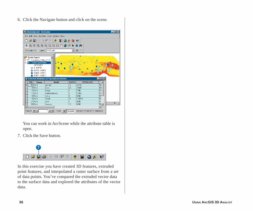
6. Click the Navigate button and click on the scene.
You can work in ArcScene while the attribute table isopen.
7. Click the Save button.
7
In this exercise you have created 3D features, extrudedpoint features, and interpolated a raster surface from a setof data points. You’ve compared the extruded vector datato the surface data and explored the attributes of the vectordata.
QUICK-START TUTORIAL 37
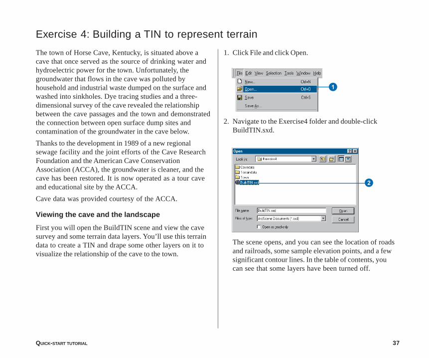
Exercise 4: Building a TIN to represent terrain
The town of Horse Cave, Kentucky, is situated above acave that once served as the source of drinking water andhydroelectric power for the town. Unfortunately, thegroundwater that flows in the cave was polluted byhousehold and industrial waste dumped on the surface andwashed into sinkholes. Dye tracing studies and a three-dimensional survey of the cave revealed the relationshipbetween the cave passages and the town and demonstratedthe connection between open surface dump sites andcontamination of the groundwater in the cave below.
Thanks to the development in 1989 of a new regionalsewage facility and the joint efforts of the Cave ResearchFoundation and the American Cave ConservationAssociation (ACCA), the groundwater is cleaner, and thecave has been restored. It is now operated as a tour caveand educational site by the ACCA.
Cave data was provided courtesy of the ACCA.
Viewing the cave and the landscape
First you will open the BuildTIN scene and view the cavesurvey and some terrain data layers. You’ll use this terraindata to create a TIN and drape some other layers on it tovisualize the relationship of the cave to the town.
1. Click File and click Open.
2. Navigate to the Exercise4 folder and double-clickBuildTIN.sxd.
The scene opens, and you can see the location of roadsand railroads, some sample elevation points, and a fewsignificant contour lines. In the table of contents, youcan see that some layers have been turned off.
1
2
38 USING ARCGIS 3D ANALYST
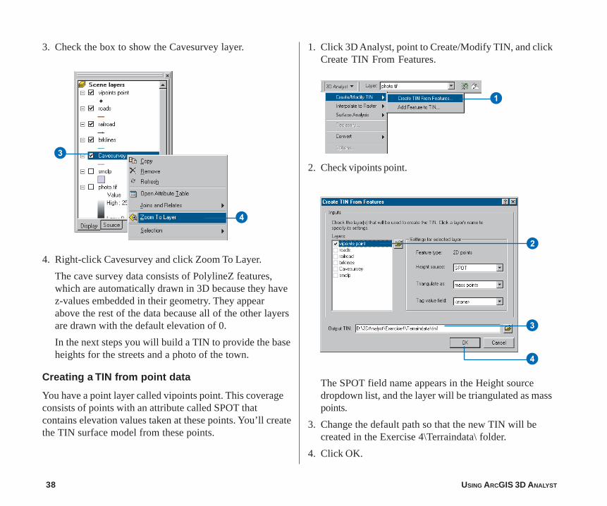
3. Check the box to show the Cavesurvey layer. 1. Click 3D Analyst, point to Create/Modify TIN, and clickCreate TIN From Features.
4. Right-click Cavesurvey and click Zoom To Layer.
The cave survey data consists of PolylineZ features,which are automatically drawn in 3D because they havez-values embedded in their geometry. They appearabove the rest of the data because all of the other layersare drawn with the default elevation of 0.
In the next steps you will build a TIN to provide the baseheights for the streets and a photo of the town.
Creating a TIN from point data
You have a point layer called vipoints point. This coverageconsists of points with an attribute called SPOT thatcontains elevation values taken at these points. You’ll createthe TIN surface model from these points.
2. Check vipoints point.
The SPOT field name appears in the Height sourcedropdown list, and the layer will be triangulated as masspoints.
3. Change the default path so that the new TIN will becreated in the Exercise 4\Terraindata\ folder.
4. Click OK.
3
4
1
2
4
3
QUICK-START TUTORIAL 39
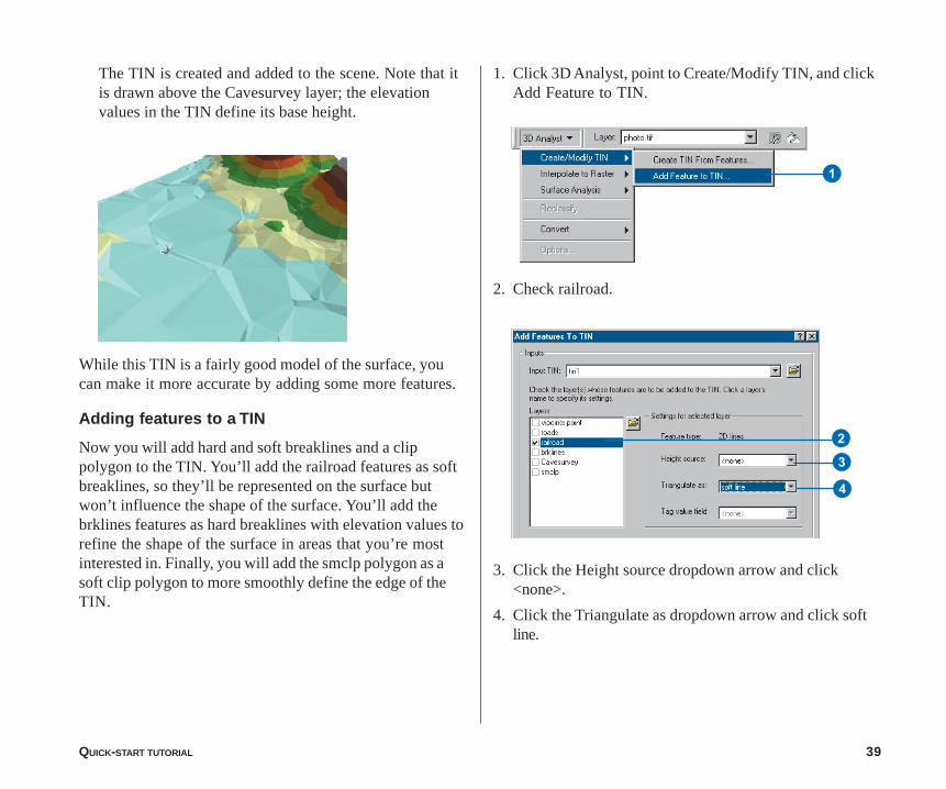
The TIN is created and added to the scene. Note that itis drawn above the Cavesurvey layer; the elevationvalues in the TIN define its base height.
1. Click 3D Analyst, point to Create/Modify TIN, and clickAdd Feature to TIN.
While this TIN is a fairly good model of the surface, youcan make it more accurate by adding some more features.
Adding features to a TIN
Now you will add hard and soft breaklines and a clippolygon to the TIN. You’ll add the railroad features as softbreaklines, so they’ll be represented on the surface butwon’t influence the shape of the surface. You’ll add thebrklines features as hard breaklines with elevation values torefine the shape of the surface in areas that you’re mostinterested in. Finally, you will add the smclp polygon as asoft clip polygon to more smoothly define the edge of theTIN.
2. Check railroad.
3. Click the Height source dropdown arrow and click<none>.
4. Click the Triangulate as dropdown arrow and click softline.
1
2
3
4

40 USING ARCGIS 3D ANALYST
5. Check brklines. 7. Click the Height source dropdown arrow and click<none>.
8. Click the Tag value field dropdown arrow and click<none>.
You have defined the feature layers that you want to addto your TIN and specified how they should be integratedinto the triangulation.
The Add Features To TIN tool detects that there is anELEVATION field and uses it for the height source. Youwill accept the default and triangulate them as hardbreaklines.
6. Check smclp.
9. Click OK.
9
7
8
6
5
QUICK-START TUTORIAL 41
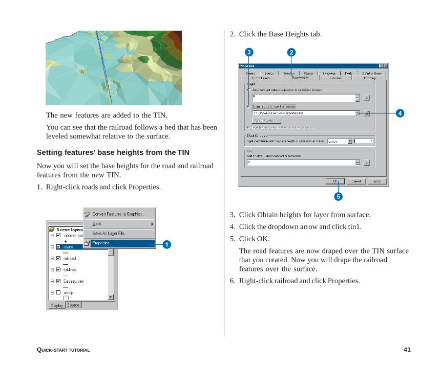
The new features are added to the TIN.
You can see that the railroad follows a bed that has beenleveled somewhat relative to the surface.
Setting features’ base heights from the TIN
Now you will set the base heights for the road and railroadfeatures from the new TIN.
1. Right-click roads and click Properties.
2. Click the Base Heights tab.
3. Click Obtain heights for layer from surface.
4. Click the dropdown arrow and click tin1.
5. Click OK.
The road features are now draped over the TIN surfacethat you created. Now you will drape the railroadfeatures over the surface.
6. Right-click railroad and click Properties.
1
23
5
4

42 USING ARCGIS 3D ANALYST
7. Click Obtain heights for layer from surface. The railroad features are now draped over the TINsurface that you created. Next you’ll drape the aerialphoto over the TIN.
Setting raster base heights from the TIN
Including the aerial photo of the town in the scene makesthe relationship between the cave and the town much moreevident. You’ll drape the raster over the TIN and make itpartly transparent so that you’ll be able to see the cavebeneath the surface.
1. Right-click photo.tif and click Properties.
8. Click OK.
6
7
8
1
QUICK-START TUTORIAL 43
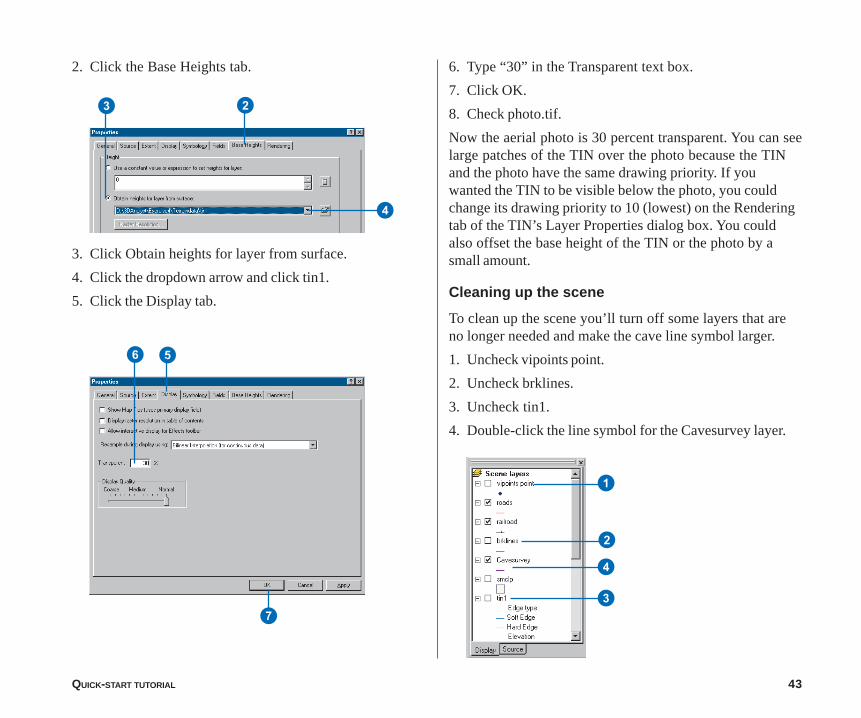
2. Click the Base Heights tab. 6. Type “30” in the Transparent text box.
7. Click OK.
8. Check photo.tif.
Now the aerial photo is 30 percent transparent. You can seelarge patches of the TIN over the photo because the TINand the photo have the same drawing priority. If youwanted the TIN to be visible below the photo, you couldchange its drawing priority to 10 (lowest) on the Renderingtab of the TIN’s Layer Properties dialog box. You couldalso offset the base height of the TIN or the photo by asmall amount.
Cleaning up the scene
To clean up the scene you’ll turn off some layers that areno longer needed and make the cave line symbol larger.
1. Uncheck vipoints point.
2. Uncheck brklines.
3. Uncheck tin1.
4. Double-click the line symbol for the Cavesurvey layer.
3. Click Obtain heights for layer from surface.
4. Click the dropdown arrow and click tin1.
5. Click the Display tab.
23
4
56
7
1
2
3
4

44 USING ARCGIS 3D ANALYST
5. Type “5” in the Width box. 1. Click the Launch ArcMap button.
6. Click OK.
Now you can see the three-dimensional passages of thecave, symbolized by thick lines. The surface featuresand the aerial photo provide context, so you can easilysee the relationship of the cave to the town.
Creating a profile of the terrain
The cave follows the valley floor orientation. To get anunderstanding of the shape of the valley, you will create aprofile across the TIN. In order to create a profile, youmust first have a 3D line (feature or graphic). You will startArcMap, copy the TIN to the map, and digitize a line tomake your profile.
ArcMap starts.
2. Click OK.
Now you will add the 3D Analyst toolbar to ArcMap. TheArcMap 3D Analyst toolbar contains a few tools that do notappear on the ArcScene 3D Analyst toolbar. Two of theseare the Interpolate Line tool and the Create Profile Graphtool, which you will use to create your profile of thesurface.
5
6
1
2
QUICK-START TUTORIAL 45
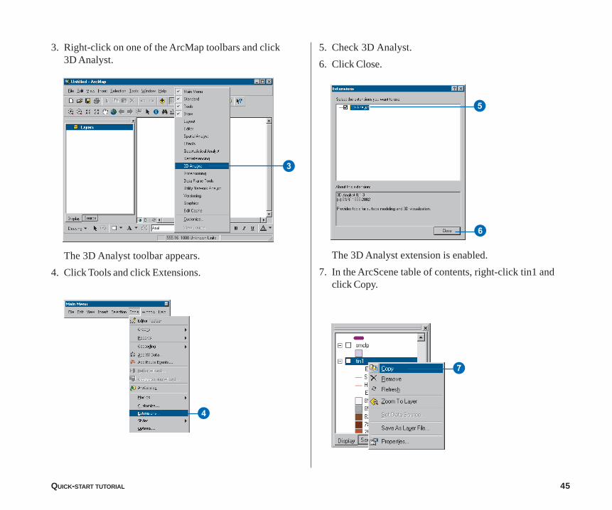
3. Right-click on one of the ArcMap toolbars and click3D Analyst.
5. Check 3D Analyst.
6. Click Close.
The 3D Analyst toolbar appears.
4. Click Tools and click Extensions.
The 3D Analyst extension is enabled.
7. In the ArcScene table of contents, right-click tin1 andclick Copy.
3
4
5
6
7
46 USING ARCGIS 3D ANALYST
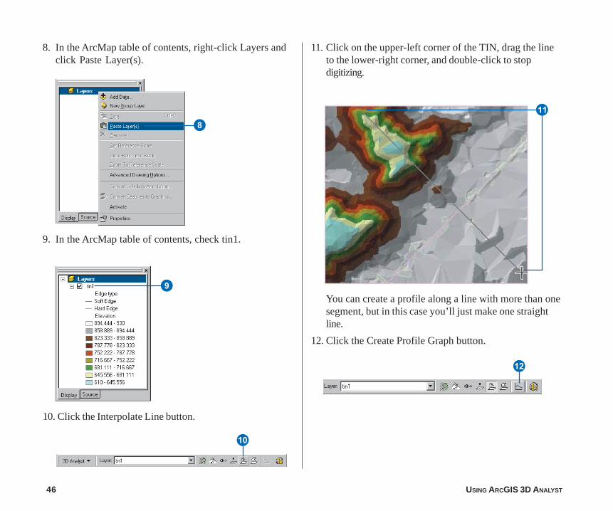
8. In the ArcMap table of contents, right-click Layers andclick Paste Layer(s).
11. Click on the upper-left corner of the TIN, drag the lineto the lower-right corner, and double-click to stopdigitizing.
Q
E
9. In the ArcMap table of contents, check tin1.
You can create a profile along a line with more than onesegment, but in this case you’ll just make one straightline.
12. Click the Create Profile Graph button.
8
9
10. Click the Interpolate Line button.
W
QUICK-START TUTORIAL 47
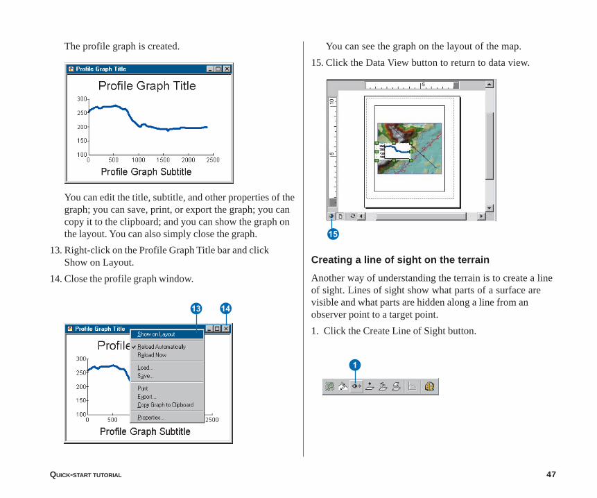
The profile graph is created. You can see the graph on the layout of the map.
15. Click the Data View button to return to data view.
1
You can edit the title, subtitle, and other properties of thegraph; you can save, print, or export the graph; you cancopy it to the clipboard; and you can show the graph onthe layout. You can also simply close the graph.
13. Right-click on the Profile Graph Title bar and clickShow on Layout.
14. Close the profile graph window.
Creating a line of sight on the terrain
Another way of understanding the terrain is to create a lineof sight. Lines of sight show what parts of a surface arevisible and what parts are hidden along a line from anobserver point to a target point.
1. Click the Create Line of Sight button.
R T
Y
48 USING ARCGIS 3D ANALYST
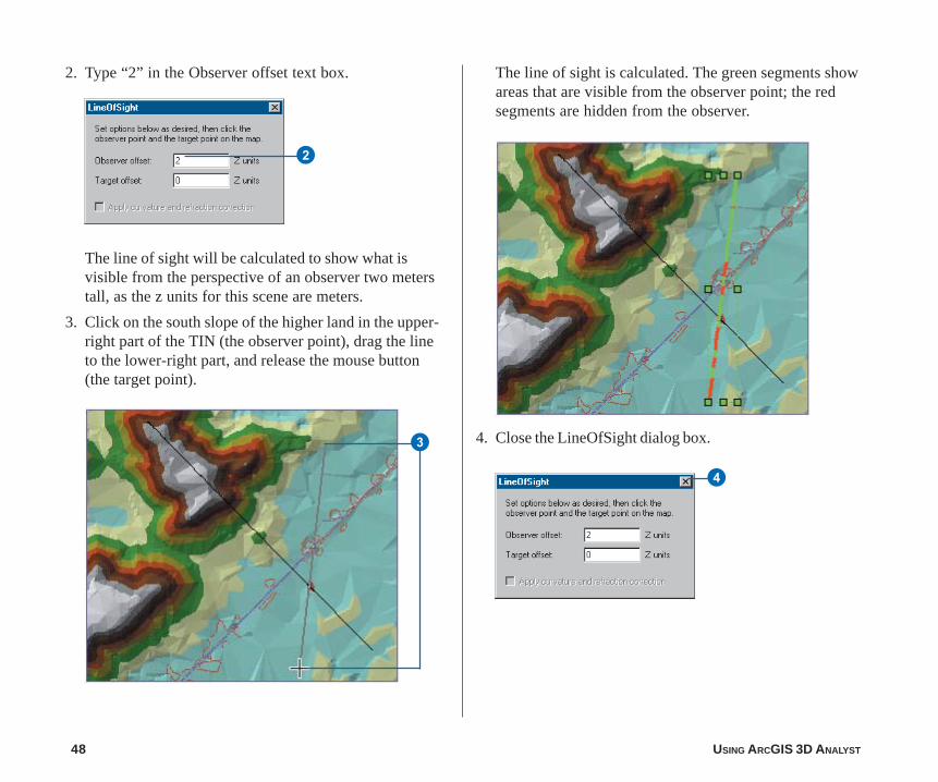
2. Type “2” in the Observer offset text box. The line of sight is calculated. The green segments showareas that are visible from the observer point; the redsegments are hidden from the observer.
The line of sight will be calculated to show what isvisible from the perspective of an observer two meterstall, as the z units for this scene are meters.
3. Click on the south slope of the higher land in the upper-right part of the TIN (the observer point), drag the lineto the lower-right part, and release the mouse button(the target point).
4. Close the LineOfSight dialog box.
2
4
3
QUICK-START TUTORIAL 49
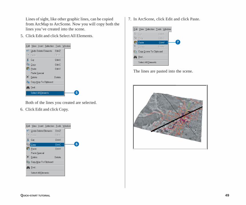
Lines of sight, like other graphic lines, can be copiedfrom ArcMap to ArcScene. Now you will copy both thelines you’ve created into the scene.
5. Click Edit and click Select All Elements.
7. In ArcScene, click Edit and click Paste.
Both of the lines you created are selected.
6. Click Edit and click Copy.
The lines are pasted into the scene.
5
6
7

50 USING ARCGIS 3D ANALYST
8. In ArcScene, click the Save button.
8
9. In ArcMap, click File and click Exit.
10. Click No.
9
Q
QUICK-START TUTORIAL 51
Exercise 5: Working with animations in ArcScene
Imagine that you wish to create an animated sequenceshowing the flight of an object over a landscape. You’vecreated a TIN and have draped images over it to show thearea. You also have some data pertaining to a strangephenomenon that has been occurring in the region. You areinterested in displaying all the data in a dynamic way,making an animation to tour points of interest, and showinghow you made the surface. You would also like to modelthe phenomenon by moving a layer in the scene.
The tutorial data has already been assembled in the scenedocument named Animation.sxd. You will use ArcSceneanimation tools to effectively convey the points you want toshow.
Data was supplied courtesy of MassGIS, Commonwealth ofMassachusetts Executive Office of Environmental Affairs.
In this exercise, you will play an existing animation in thescene document, Final Animation_A.sxd, and perform thetasks typically used to create the animation.
Opening the Final Animation_A scene document
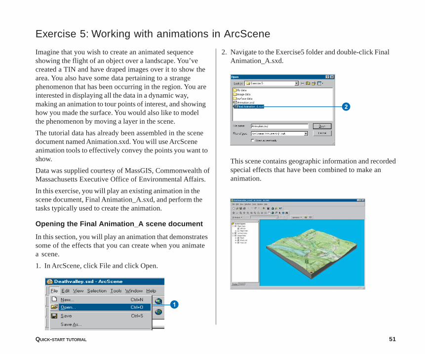
In this section, you will play an animation that demonstratessome of the effects that you can create when you animatea scene.
1. In ArcScene, click File and click Open.
2. Navigate to the Exercise5 folder and double-click FinalAnimation_A.sxd.
2
This scene contains geographic information and recordedspecial effects that have been combined to make ananimation.
1

52 USING ARCGIS 3D ANALYST
This animation shows the flight of a hypotheticalunidentified flying object (UFO) over the terrain.
3. Click the Play button.
Playing the scene’s animation
In order to view a scene’s animation, you need to turn onthe Animation toolbar.
1. Click View, point to Toolbars, and click Animation.
The Animation toolbar appears. Now you’ll play theanimation.
2. Click the Open Animation Controls button.
The animation plays, illustrating some of the effects youcan use in an animated scene.
In the next section you will work through the steps usedto make animations like this one.
3
2
1
QUICK-START TUTORIAL 53
Opening the Animation scene document
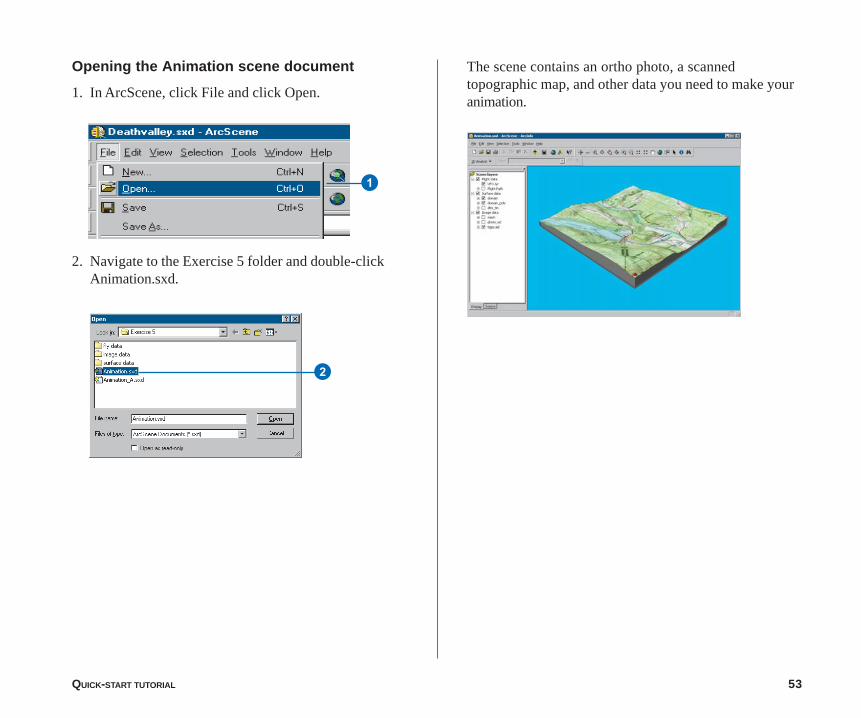
1. In ArcScene, click File and click Open.
The scene contains an ortho photo, a scannedtopographic map, and other data you need to make youranimation.
2. Navigate to the Exercise 5 folder and double-clickAnimation.sxd.
1
2
54 USING ARCGIS 3D ANALYST
For a camera keyframe, the object is the virtual camerathrough which you view the scene. Navigating the scenechanges camera properties that determine its position.
ArcScene interpolates a camera path betweenkeyframes, so you’ll need to capture more views tomake a track that shows animation.
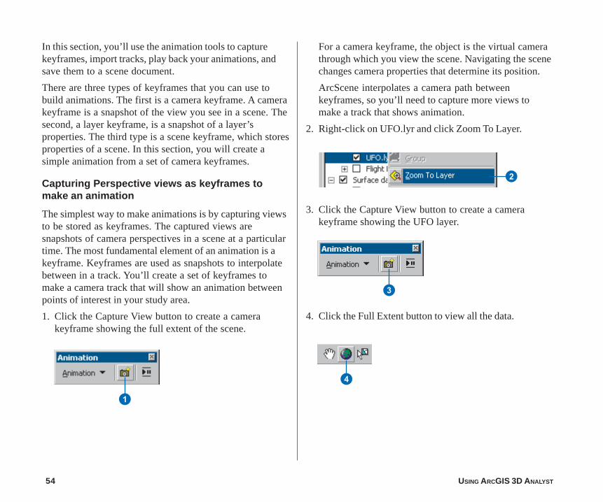
2. Right-click on UFO.lyr and click Zoom To Layer.
In this section, you’ll use the animation tools to capturekeyframes, import tracks, play back your animations, andsave them to a scene document.
There are three types of keyframes that you can use tobuild animations. The first is a camera keyframe. A camerakeyframe is a snapshot of the view you see in a scene. Thesecond, a layer keyframe, is a snapshot of a layer’sproperties. The third type is a scene keyframe, which storesproperties of a scene. In this section, you will create asimple animation from a set of camera keyframes.
Capturing Perspective views as keyframes tomake an animation
The simplest way to make animations is by capturing viewsto be stored as keyframes. The captured views aresnapshots of camera perspectives in a scene at a particulartime. The most fundamental element of an animation is akeyframe. Keyframes are used as snapshots to interpolatebetween in a track. You’ll create a set of keyframes tomake a camera track that will show an animation betweenpoints of interest in your study area.
1. Click the Capture View button to create a camerakeyframe showing the full extent of the scene.
1
3
4
3. Click the Capture View button to create a camerakeyframe showing the UFO layer.
4. Click the Full Extent button to view all the data.
2
QUICK-START TUTORIAL 55
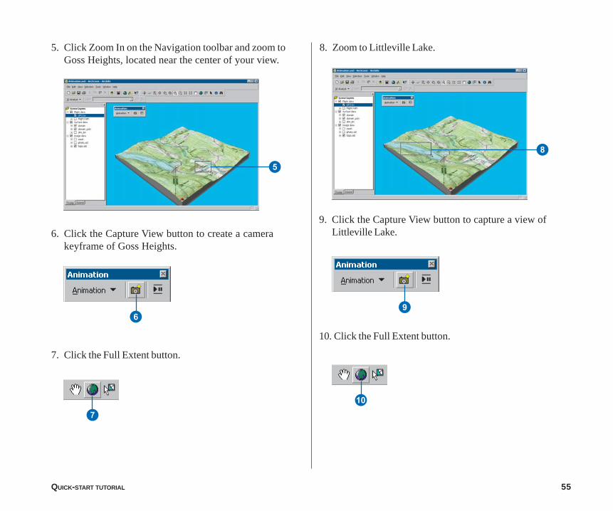
8. Zoom to Littleville Lake.5. Click Zoom In on the Navigation toolbar and zoom toGoss Heights, located near the center of your view.
5
6
7
8
9
Q
6. Click the Capture View button to create a camerakeyframe of Goss Heights.
7. Click the Full Extent button.
9. Click the Capture View button to capture a view ofLittleville Lake.
10. Click the Full Extent button.
56 USING ARCGIS 3D ANALYST
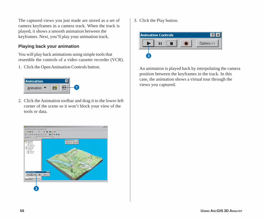
The captured views you just made are stored as a set ofcamera keyframes in a camera track. When the track isplayed, it shows a smooth animation between thekeyframes. Next, you’ll play your animation track.
Playing back your animation
You will play back animations using simple tools thatresemble the controls of a video cassette recorder (VCR).
1. Click the Open Animation Controls button.
1
3. Click the Play button.
3
2. Click the Animation toolbar and drag it to the lower-leftcorner of the scene so it won’t block your view of thetools or data.
An animation is played back by interpolating the cameraposition between the keyframes in the track. In thiscase, the animation shows a virtual tour through theviews you captured.
2
QUICK-START TUTORIAL 57
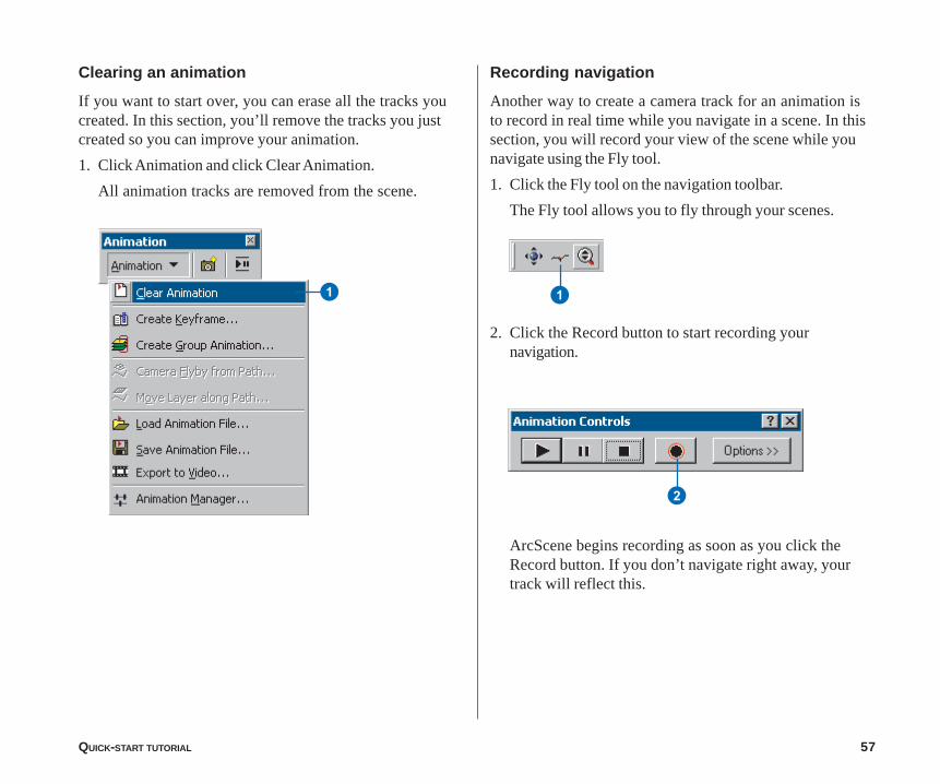
Clearing an animation
If you want to start over, you can erase all the tracks youcreated. In this section, you’ll remove the tracks you justcreated so you can improve your animation.
1. Click Animation and click Clear Animation.
All animation tracks are removed from the scene.
Recording navigation
Another way to create a camera track for an animation isto record in real time while you navigate in a scene. In thissection, you will record your view of the scene while younavigate using the Fly tool.
1. Click the Fly tool on the navigation toolbar.
The Fly tool allows you to fly through your scenes.
1
2
2. Click the Record button to start recording yournavigation.
ArcScene begins recording as soon as you click theRecord button. If you don’t navigate right away, yourtrack will reflect this.
1
58 USING ARCGIS 3D ANALYST
Exercise 6: ArcGlobe basics
Learning how to navigate in ArcGlobe helps you understandhow you can explore your data and teaches you how toaccomplish fundamental tasks that you will use as yourArcGlobe experience grows.
In this exercise you’ll learn how to use the ArcGlobenavigation tools and how to set properties that enhance yourviewing experience. This exercise assumes that you areusing ESRI-supplied default layers.
Examining the default layers in ArcGlobe
First, you’ll open ArcGlobe and learn what kind of data isincluded with ArcGlobe by default.
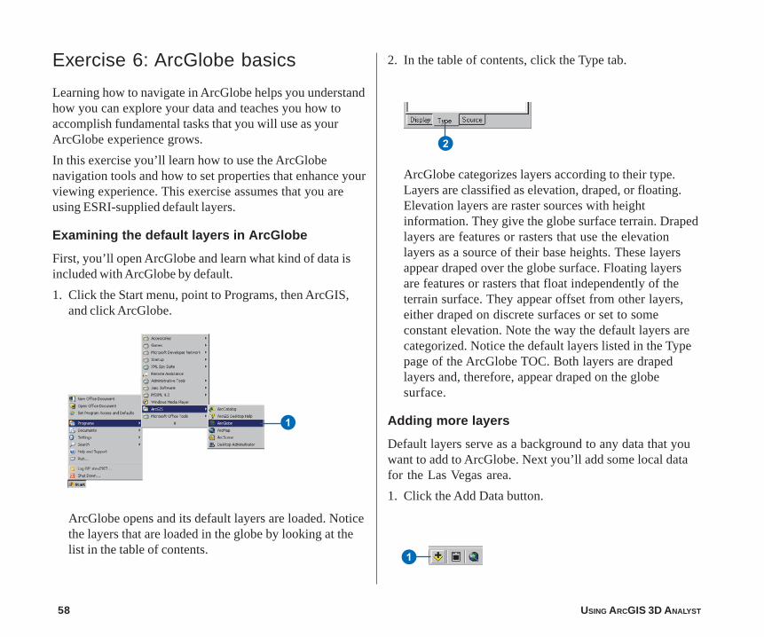
1. Click the Start menu, point to Programs, then ArcGIS,and click ArcGlobe.
ArcGlobe opens and its default layers are loaded. Noticethe layers that are loaded in the globe by looking at thelist in the table of contents.
2. In the table of contents, click the Type tab.
ArcGlobe categorizes layers according to their type.Layers are classified as elevation, draped, or floating.Elevation layers are raster sources with heightinformation. They give the globe surface terrain. Drapedlayers are features or rasters that use the elevationlayers as a source of their base heights. These layersappear draped over the globe surface. Floating layersare features or rasters that float independently of theterrain surface. They appear offset from other layers,either draped on discrete surfaces or set to someconstant elevation. Note the way the default layers arecategorized. Notice the default layers listed in the Typepage of the ArcGlobe TOC. Both layers are drapedlayers and, therefore, appear draped on the globesurface.
Adding more layers
Default layers serve as a background to any data that youwant to add to ArcGlobe. Next you’ll add some local datafor the Las Vegas area.
1. Click the Add Data button.
1
1
2
QUICK-START TUTORIAL 59
2. Navigate to the location of the Exercise 6 tutorial datafolder.
3. Click las_vegas_area.img, press Shift, and clicklas_vegas_strip.img.
The layers are multiply selected.
4. Click Add.
The image layers are added to ArcGlobe as drapedlayers. You’ll explore them later in the exercise.
Changing a layer’s drawing priority in the table ofcontents
Draped layers that have overlapping extents need to have adrawing priority set so one layer gets drawn on top of theother. ArcGlobe makes some guesses to accomplish this,using criteria such as the cell size of a raster layer.Occasionally, you’ll need to override the ArcGlobe defaultdrawing priorities. One way to do this is to change the orderof draped layers as they appear in the Type page of thetable of contents.
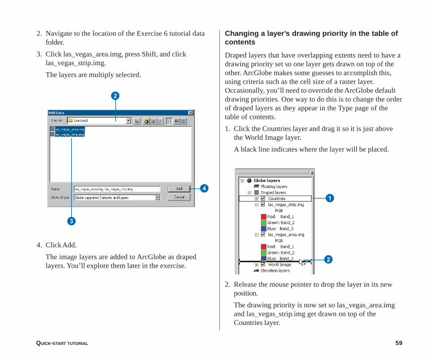
1. Click the Countries layer and drag it so it is just abovethe World Image layer.
A black line indicates where the layer will be placed.
2. Release the mouse pointer to drop the layer in its newposition.
The drawing priority is now set so las_vegas_area.imgand las_vegas_strip.img get drawn on top of theCountries layer.
1
2
2
3
4
60 USING ARCGIS 3D ANALYST
Navigate
Zoom In/Out
1
2
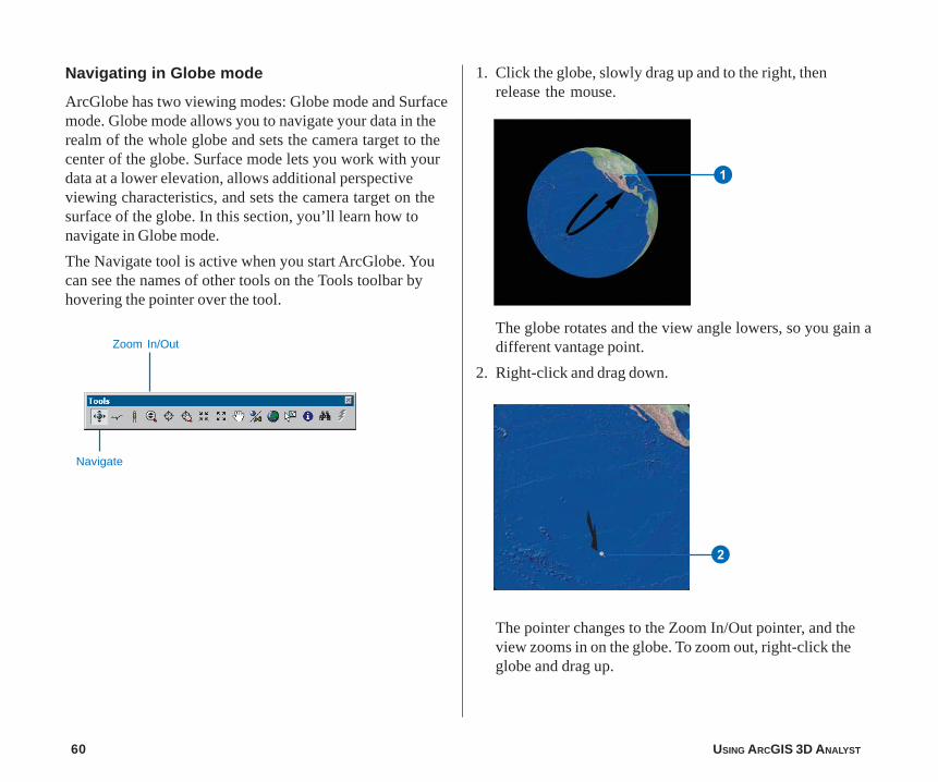
1. Click the globe, slowly drag up and to the right, thenrelease the mouse.
The globe rotates and the view angle lowers, so you gain adifferent vantage point.
2. Right-click and drag down.
The pointer changes to the Zoom In/Out pointer, and theview zooms in on the globe. To zoom out, right-click theglobe and drag up.
Navigating in Globe mode
ArcGlobe has two viewing modes: Globe mode and Surfacemode. Globe mode allows you to navigate your data in therealm of the whole globe and sets the camera target to thecenter of the globe. Surface mode lets you work with yourdata at a lower elevation, allows additional perspectiveviewing characteristics, and sets the camera target on thesurface of the globe. In this section, you’ll learn how tonavigate in Globe mode.
The Navigate tool is active when you start ArcGlobe. Youcan see the names of other tools on the Tools toolbar byhovering the pointer over the tool.
QUICK-START TUTORIAL 61
1
3
3. Click Full Extent.
The globe displays at full extent.
Turning on the Spin toolbar
You can use the Spin toolbar to automatically spin the globeclockwise or counterclockwise at any speed you wish.
1. Right-click in the menu area and click Spin.
The Spin toolbar appears as an undocked toolbar.
2
3
Using the Spin tools
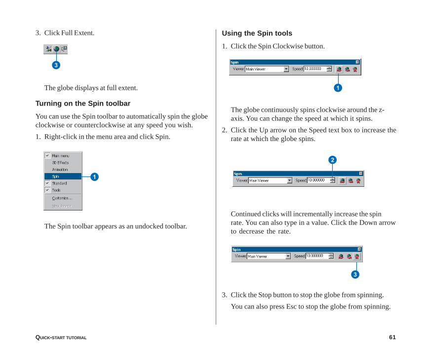
1. Click the Spin Clockwise button.
The globe continuously spins clockwise around the z-axis. You can change the speed at which it spins.
2. Click the Up arrow on the Speed text box to increase therate at which the globe spins.
Continued clicks will incrementally increase the spinrate. You can also type in a value. Click the Down arrowto decrease the rate.
3. Click the Stop button to stop the globe from spinning.
You can also press Esc to stop the globe from spinning.
1
62 USING ARCGIS 3D ANALYST
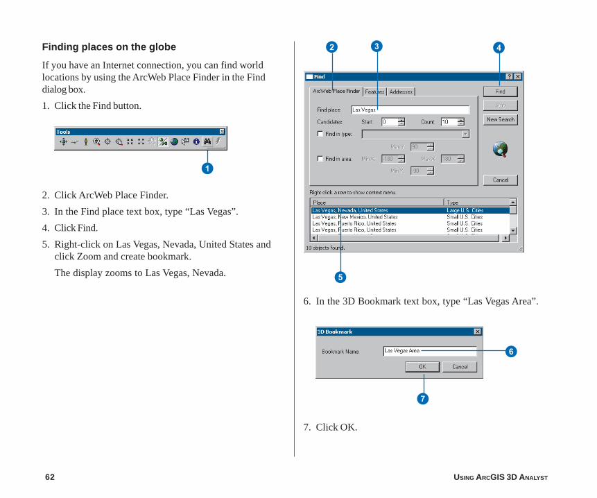
Finding places on the globe
If you have an Internet connection, you can find worldlocations by using the ArcWeb Place Finder in the Finddialog box.
1. Click the Find button.
2. Click ArcWeb Place Finder.
3. In the Find place text box, type “Las Vegas”.
4. Click Find.
5. Right-click on Las Vegas, Nevada, United States andclick Zoom and create bookmark.
The display zooms to Las Vegas, Nevada.
6. In the 3D Bookmark text box, type “Las Vegas Area”.
7. Click OK.
1
2 3 4
5
6
7
QUICK-START TUTORIAL 63
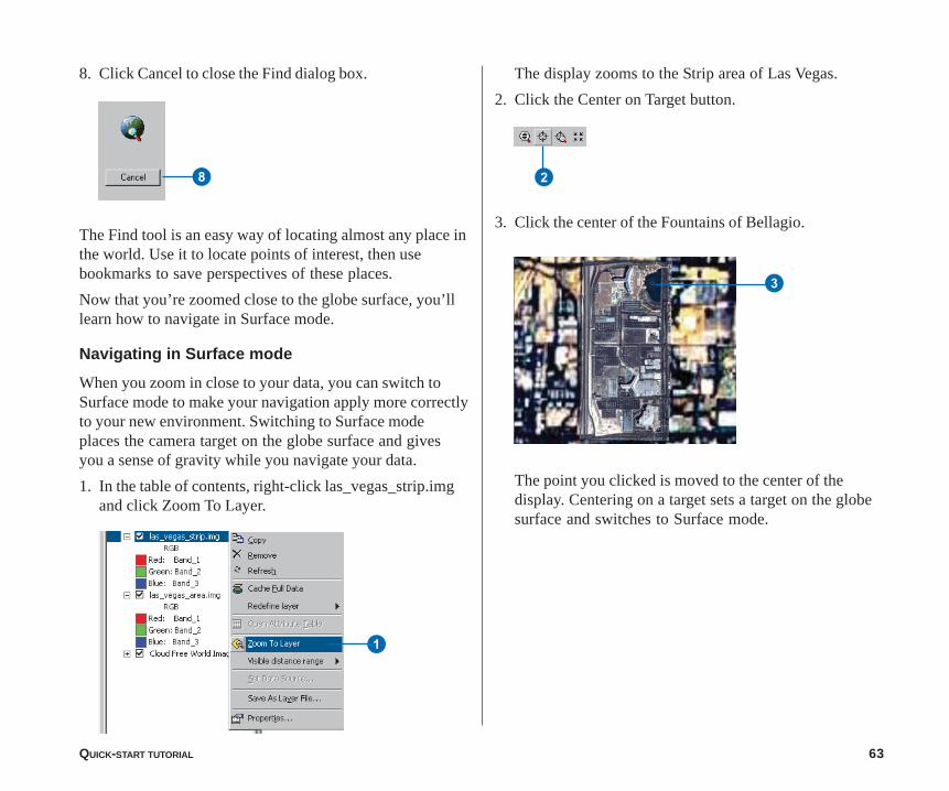
8. Click Cancel to close the Find dialog box.
The Find tool is an easy way of locating almost any place inthe world. Use it to locate points of interest, then usebookmarks to save perspectives of these places.
Now that you’re zoomed close to the globe surface, you’lllearn how to navigate in Surface mode.
Navigating in Surface mode
When you zoom in close to your data, you can switch toSurface mode to make your navigation apply more correctlyto your new environment. Switching to Surface modeplaces the camera target on the globe surface and givesyou a sense of gravity while you navigate your data.
1. In the table of contents, right-click las_vegas_strip.imgand click Zoom To Layer.
8
The display zooms to the Strip area of Las Vegas.
2. Click the Center on Target button.
3. Click the center of the Fountains of Bellagio.
The point you clicked is moved to the center of thedisplay. Centering on a target sets a target on the globesurface and switches to Surface mode.
1
2
3
64 USING ARCGIS 3D ANALYST
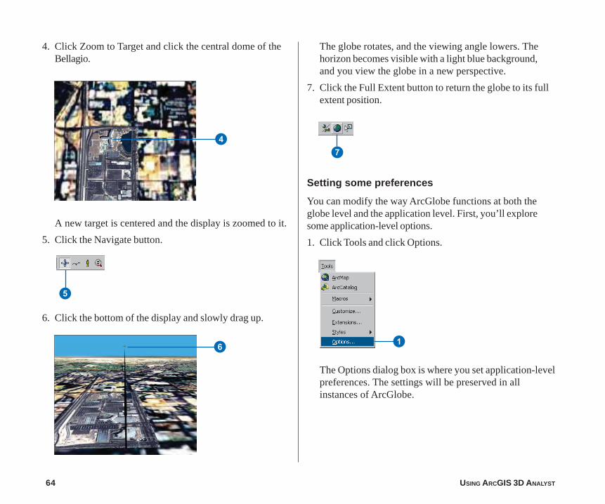
4. Click Zoom to Target and click the central dome of theBellagio.
A new target is centered and the display is zoomed to it.
5. Click the Navigate button.
6. Click the bottom of the display and slowly drag up.
The globe rotates, and the viewing angle lowers. Thehorizon becomes visible with a light blue background,and you view the globe in a new perspective.
7. Click the Full Extent button to return the globe to its fullextent position.
Setting some preferences
You can modify the way ArcGlobe functions at both theglobe level and the application level. First, you’ll exploresome application-level options.
1. Click Tools and click Options.
The Options dialog box is where you set application-levelpreferences. The settings will be preserved in allinstances of ArcGlobe.
7
1
4
6
5
QUICK-START TUTORIAL 65
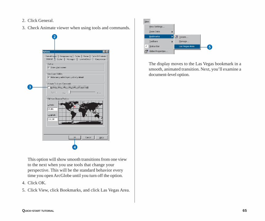
2. Click General.
3. Check Animate viewer when using tools and commands.
This option will show smooth transitions from one viewto the next when you use tools that change yourperspective. This will be the standard behavior everytime you open ArcGlobe until you turn off the option.
4. Click OK.
5. Click View, click Bookmarks, and click Las Vegas Area.
5
3
4
2
The display moves to the Las Vegas bookmark in asmooth, animated transition. Next, you’ll examine adocument-level option.
66 USING ARCGIS 3D ANALYST
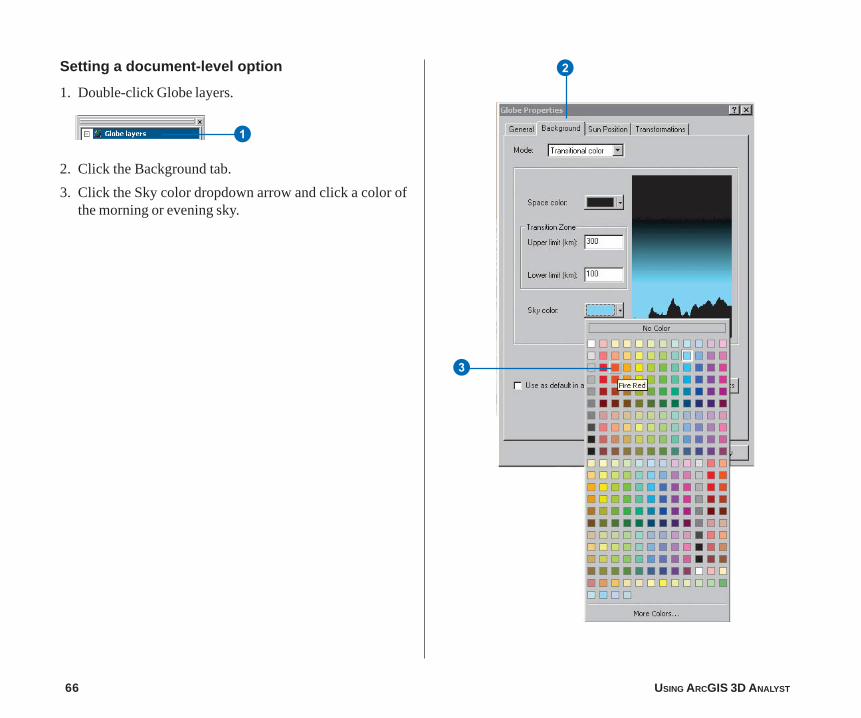
Setting a document-level option
1. Double-click Globe layers.
2. Click the Background tab.
3. Click the Sky color dropdown arrow and click a color ofthe morning or evening sky.
1
2
3

QUICK-START TUTORIAL 67
Sky color is the color of the background when you zoomin close to your globe as defined by the lower limit of thetransition zone.
4. Click OK.
If you switch to Surface mode and lower the viewingangle, you’ll notice the background color changing to thecolor you indicated. Use different background colors toconvey different moods.
In this exercise you’ve learned how to differentiatebetween ArcGlobe layer types, navigate in Surface andGlobe modes, find places, and set some application andglobe properties. Now that you’ve learned somefundamentals, you can begin to explore other areas ofArcGlobe. In the next exercise, you’ll learn how to use dataas different layer categories.
4
68 USING ARCGIS 3D ANALYST
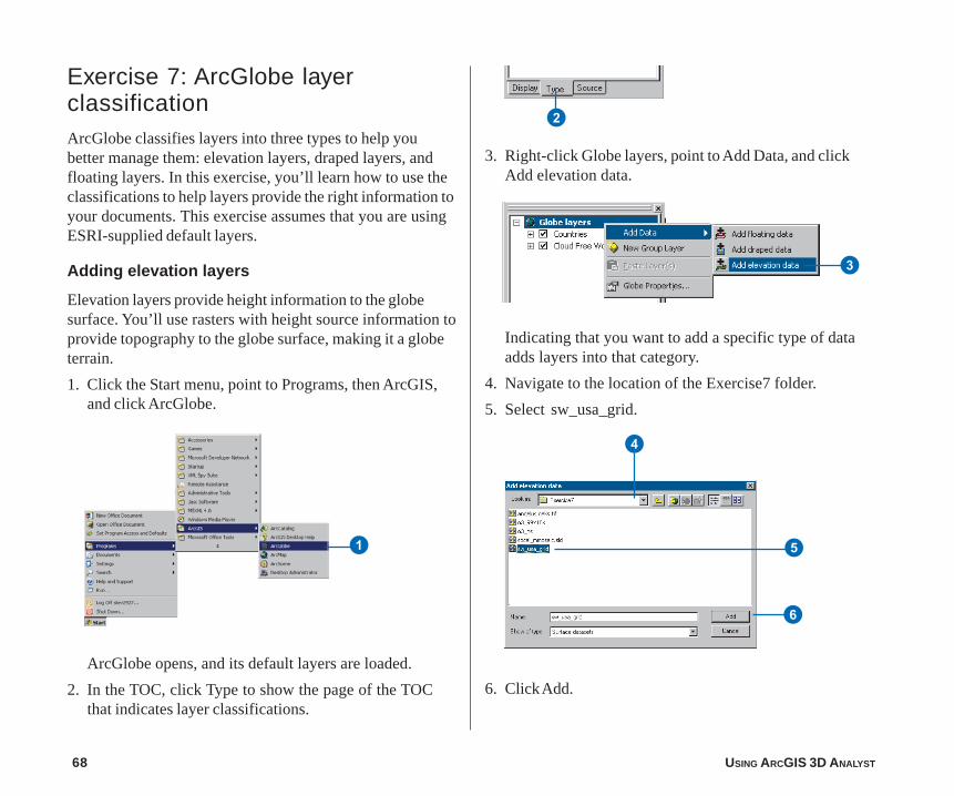
Exercise 7: ArcGlobe layerclassificationArcGlobe classifies layers into three types to help youbetter manage them: elevation layers, draped layers, andfloating layers. In this exercise, you’ll learn how to use theclassifications to help layers provide the right information toyour documents. This exercise assumes that you are usingESRI-supplied default layers.
Adding elevation layers
Elevation layers provide height information to the globesurface. You’ll use rasters with height source information toprovide topography to the globe surface, making it a globeterrain.
1. Click the Start menu, point to Programs, then ArcGIS,and click ArcGlobe.
ArcGlobe opens, and its default layers are loaded.
2. In the TOC, click Type to show the page of the TOCthat indicates layer classifications.
1
2
3. Right-click Globe layers, point to Add Data, and clickAdd elevation data.
Indicating that you want to add a specific type of dataadds layers into that category.
4. Navigate to the location of the Exercise7 folder.
5. Select sw_usa_grid.
6. Click Add.
3
4
5
6
QUICK-START TUTORIAL 69
The raster is added to the Elevation category and will beused as a source of elevation for the globe surface.
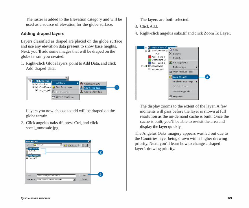
Adding draped layers
Layers classified as draped are placed on the globe surfaceand use any elevation data present to show base heights.Next, you’ll add some images that will be draped on theglobe terrain you created.
1. Right-click Globe layers, point to Add Data, and clickAdd draped data.
Layers you now choose to add will be draped on theglobe terrain.
2. Click angelus oaks.tif, press Ctrl, and clicksocal_mmosaic.jpg.
The layers are both selected.
3. Click Add.
4. Right-click angelus oaks.tif and click Zoom To Layer.
The display zooms to the extent of the layer. A fewmoments will pass before the layer is shown at fullresolution as the on-demand cache is built. Once thecache is built, you’ll be able to revisit the area anddisplay the layer quickly.
The Angelus Oaks imagery appears washed out due tothe Countries layer being drawn with a higher drawingpriority. Next, you’ll learn how to change a drapedlayer’s drawing priority.
1
4
2
3

70 USING ARCGIS 3D ANALYST
Changing a layer’s drawing priority in the table ofcontents
Draped layers that have overlapping extents need to have adrawing priority set so one layer gets drawn on top of theother. ArcGlobe makes some guesses to accomplish this,using criteria such as the cell size of a raster layer.Occasionally, you’ll need to override the ArcGlobe defaultdrawing priorities. One way to do this is to change the orderof draped layers as they appear in the Type page of thetable of contents.
1. Click the Countries layer and drag it so it is just abovethe World Image layer.
A black line indicates where the layer will be placed.
2. Release the mouse pointer to drop the layer in its newposition.
The drawing priority is now set so angelus oaks.tif andsocal_mmosaic.sid get drawn on top of the Countrieslayer.
1
2
Setting a target to initiate Surface mode
1. Press Ctrl and click in the middle of the display.
You’ve initiated Surface mode and set a target at thelocation on the globe surface where you clicked.
1
QUICK-START TUTORIAL 71
2
3
1
2
3
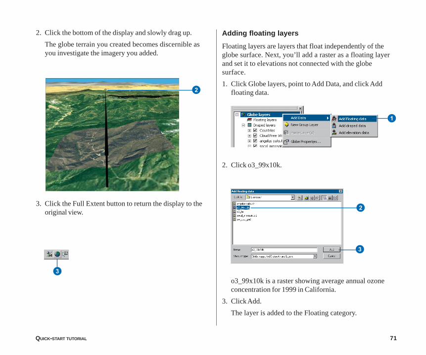
Adding floating layers
Floating layers are layers that float independently of theglobe surface. Next, you’ll add a raster as a floating layerand set it to elevations not connected with the globesurface.
1. Click Globe layers, point to Add Data, and click Addfloating data.
2. Click o3_99x10k.
o3_99x10k is a raster showing average annual ozoneconcentration for 1999 in California.
3. Click Add.
The layer is added to the Floating category.
2. Click the bottom of the display and slowly drag up.
The globe terrain you created becomes discernible asyou investigate the imagery you added.
3. Click the Full Extent button to return the display to theoriginal view.
72 USING ARCGIS 3D ANALYST
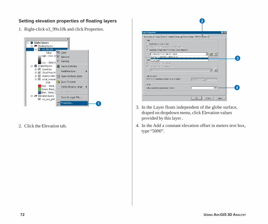
Setting elevation properties of floating layers
1. Right-click o3_99x10k and click Properties.
2. Click the Elevation tab.
1 3. In the Layer floats independent of the globe surface,draped on dropdown menu, click Elevation valuesprovided by this layer .
4. In the Add a constant elevation offset in meters text box,type “5000”.
2
3
4
QUICK-START TUTORIAL 73
1
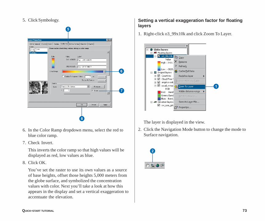
5. Click Symbology.
6. In the Color Ramp dropdown menu, select the red toblue color ramp.
7. Check Invert.
This inverts the color ramp so that high values will bedisplayed as red, low values as blue.
8. Click OK.
You’ve set the raster to use its own values as a sourceof base heights, offset those heights 5,000 meters fromthe globe surface, and symbolized the concentrationvalues with color. Next you’ll take a look at how thisappears in the display and set a vertical exaggeration toaccentuate the elevation.
5
6
7
8
2
Setting a vertical exaggeration factor for floatinglayers
1. Right-click o3_99x10k and click Zoom To Layer.
The layer is displayed in the view.
2. Click the Navigation Mode button to change the mode toSurface navigation.
74 USING ARCGIS 3D ANALYST
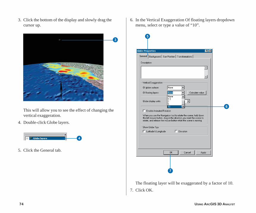
3. Click the bottom of the display and slowly drag thecursor up.
This will allow you to see the effect of changing thevertical exaggeration.
4. Double-click Globe layers.
5. Click the General tab.
3
4
6. In the Vertical Exaggeration Of floating layers dropdownmenu, select or type a value of “10”.
The floating layer will be exaggerated by a factor of 10.
7. Click OK.
5
6
7

QUICK-START TUTORIAL 75
Examine the floating layer you’ve created. You’ll see a3D raster showing average ozone concentrations inCalifornia in 1999. The layer floats above the state ofCalifornia and is a surface that is different from theterrain below.
In this exercise, you learned how to differentiate layer typesin ArcGlobe, saw the effect they have on the globe, and setproperties to improve their display. Explore Exercise7.3ddglobe document in the Exercise7 folder to discoveradditional ways to enhance your globe documents. Thedocument contains layers saved with custom settings,bookmarks, globe lighting, and animation tracks.
