tutorials for the hydrus wetland module - pc-progress · tutorials for the hydrus wetland module...

Computer Session

of 44

TUTORIALS FOR THE HYDRUS WETLAND MODULE

These tutorials show the use of the HYDRUS Wetland Module (Langergraber and Šimůnek, 2006, 2011) for simulating vertical flow (VF) and horizontal flow (HF) wetlands. The following tutorials are provided in this section.

1) Water Flow in a Vertical Flow Wetland.

2) Reactive Transport in a Vertical Flow Wetland (HYDRUS Wetland Module, CW2D Biokinetic Model).

3) Water Flow and Reactive Transport in a Horizontal Flow Wetland (HYDRUS Wetland Module, CWM1 Biokinetic Model).

Computer Session

of 44

References:

Langergraber, G. and J. Šimůnek, Modeling variably-saturated water flow and multi-component reactive transport in constructed wetlands, Vadose Zone Journal 4, 924-938, 2005.

Langergraber, G., and J. Šimůnek, The multi-component reactive transport module CW2D for constructed wetlands for the HYDRUS Software Package. Hydrus Software Series 2, Department of Environmental Sciences, University of California Riverside, Riverside, California, USA, 72p., 2006.

Langergraber, G., D. Rousseau, J. García, and J. Mena, CWM1 - A general model to describe biokinetic processes in subsurface flow constructed wetlands. Water Sci Technol 59(9), 1687-1697, 2009.

Langergraber, G., and J. Šimůnek, HYDRUS Wetland Module, Version 2. Hydrus Software Series 4, Department of Environmental Sciences, University of California Riverside, Riverside, California, USA, 56p., 2011.

Langergraber, G., Šimůnek, J. (2012): Reactive Transport Modeling of Subsurface Flow Constructed Wetlands Using the HYDRUS Wetland Module. Vadoze Zone Journal 11(2) Special Issue "Reactive Transport Modeling", doi:10.2136/vzj2011.0104.

Computer Session

of 44

1 Water Flow in a Vertical Flow Wetland

This example shows the set-up of flow simulations in a VF wetland and the calibration of the flow model using measurements of the volumetric effluent flow rate. The example is based on the one provided in Langergraber and Šimůnek (2006).

The example consists of the five following steps:

1. Project set up, a 24-h long simulation with 4 loadings of 3-min duration. 2. Simulation is repeated (with the initial conditions obtained in the previous step) to

reach pseudo steady-state conditions for water flow. 3. Calibration of soil hydraulic parameters against measured outflow data. 4. Simulation is re-run with the new (calibrated) soil hydraulic parameters. 5. Simulation is repeated (with the initial conditions obtained in the previous step and

new soil hydraulic parameters) to reach pseudo steady-state conditions.

1.1 System Description

The VF wetland has a surface area of 1 m² (1x1 m²), a height of the main layer of the filter bed is 50 cm. The main layer consists of sand (gravel size 0.06-4 mm). An intermediate layer of 10 cm thickness with a gravel size of 4-8 mm prevents fine particles to be washed out into the drainage layer (15 cm thick; gravel 16-32 cm) where the effluent is collected by means of tile drains.

The sandy material used for the main layer has a porosity of 0.30 and the saturated hydraulic conductivity, Ks, of 117 cm/h. Table 1 shows the measured cumulated effluent flow for one loading interval of 6 hours and a single hydraulic loading of 10 L. The duration of a single loading is 3 minutes.

Table 1. Measured cumulated volumetric effluent flow

Time [min] 20 40 60 80 100 120 140 160 180 200 240 Cum. effluent [L] 0.31 0.64 0.99 1.49 2.36 3.14 3.95 4.75 5.47 6.14 7.31 Time [min] 270 300 330 360 Cum. effluent [L] 8.08 8.78 9.43 9.99

Only the 50 cm main layer of the VF bed shall be considered in the simulation.

Computer Session

of 44

1.2 The HYDRUS Project Setup

Simulation 1 - Set-up:

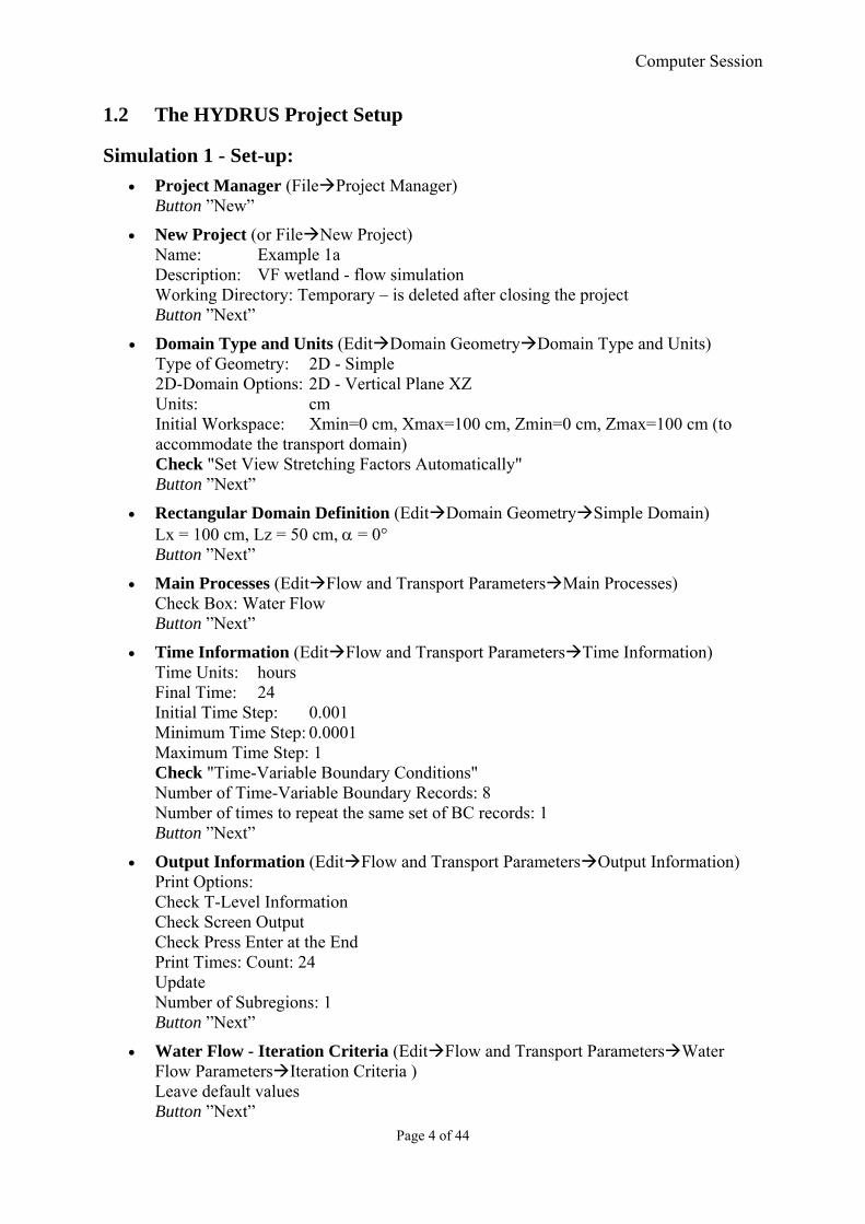
Project Manager (FileProject Manager) Button ”New”

New Project (or FileNew Project) Name: Example 1a Description: VF wetland - flow simulation Working Directory: Temporary – is deleted after closing the project Button ”Next”

Domain Type and Units (EditDomain GeometryDomain Type and Units) Type of Geometry: 2D - Simple 2D-Domain Options: 2D - Vertical Plane XZ Units: cm Initial Workspace: Xmin=0 cm, Xmax=100 cm, Zmin=0 cm, Zmax=100 cm (to accommodate the transport domain) Check "Set View Stretching Factors Automatically" Button ”Next”

Rectangular Domain Definition (EditDomain GeometrySimple Domain) Lx = 100 cm, Lz = 50 cm, = 0° Button ”Next”

Main Processes (EditFlow and Transport ParametersMain Processes) Check Box: Water Flow Button ”Next”

Time Information (EditFlow and Transport ParametersTime Information) Time Units: hours Final Time: 24 Initial Time Step: 0.001 Minimum Time Step: 0.0001 Maximum Time Step: 1 Check "Time-Variable Boundary Conditions" Number of Time-Variable Boundary Records: 8 Number of times to repeat the same set of BC records: 1 Button ”Next”

Output Information (EditFlow and Transport ParametersOutput Information) Print Options: Check T-Level Information Check Screen Output Check Press Enter at the End Print Times: Count: 24 Update Number of Subregions: 1 Button ”Next”

Water Flow - Iteration Criteria (EditFlow and Transport ParametersWater Flow ParametersIteration Criteria ) Leave default values Button ”Next”

Computer Session

of 44

Water Flow – Soil-Hydraulic Model (EditFlow and Transport ParametersWater Flow ParametersHydraulic Properties Model) Radio button - van Genuchten-Mualem Radio button - No hysteresis Button ”Next”

Water Flow - Soil-Hydraulic Params (EditFlow and Transport ParametersWater Flow ParametersSoil Hydraulic Parameters) Select "Sand" from Soil Catalog Enter measured values for Qs = 0.30 and Ks = 117 cm/h Button ”Next”

Time-Variable Boundary Conditions (EditFlow and Transport ParametersVariably Boundary Conditions) Calculations: duration of a single loading: 3 minutes = 0.05 hours amount of a single loading: 10 L/m² = 10 mm = 1 cm actual loading rate: 1 cm / 0.05 h = 20 cm/h Time-Variable Boundary Conditions:

Time Precip. Evap. Transp. hCritA [hours] [cm/h] [cm/h] [cm/h] [cm] 1 0.05 20 0 0 10000 Remaining columns = 0 2 6 0 0 0 10000 3 6.05 20 0 0 10000 4 12 0 0 0 10000 5 12.05 20 0 0 10000 6 18 0 0 0 10000 7 18.05 20 0 0 10000 8 24 0 0 0 10000

Button ”Next”

FE-Mesh - FE-Mesh Parameters (EditFE-MeshFE-Mesh Parameters) horizontal Discretization in X: Count = 11 Button "Update" horizontal Discretization in Z: Count = 21 Button "Update" Generate Z-Coordinates: RS2 = 4 Button "Generate" Button ”OK”

Water Flow Initial Conditions: Click on the Initial Conditions Tab under the View Window. Or on the Navigator Bar click on Initial Conditions – Pressure Head (or InsertInitial ConditionsPressure Head) Select the entire transport domain and click on the Set Pressure Head IC command at the Edit Bar, check Hydrostatic equilibrium from the lowest located nodal point, check that Bottom Pressure Head Value is set equal to -2 cm. Button ”OK”

Computer Session

of 44

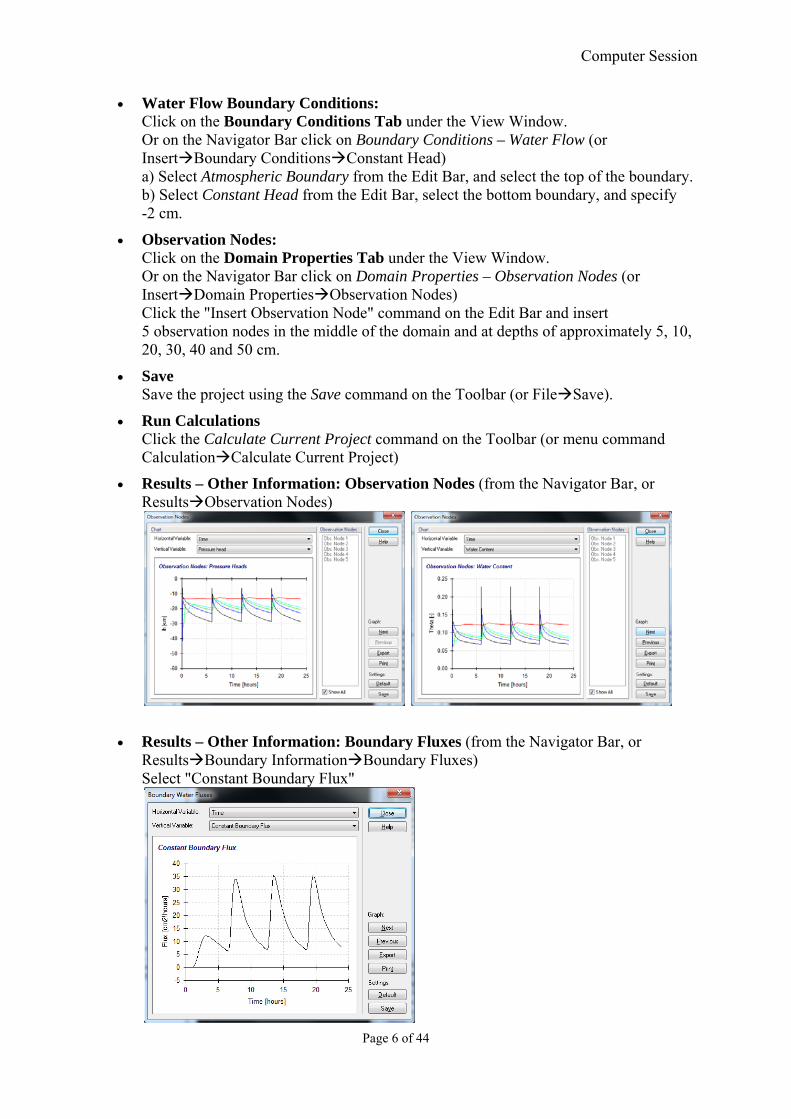
Water Flow Boundary Conditions: Click on the Boundary Conditions Tab under the View Window. Or on the Navigator Bar click on Boundary Conditions – Water Flow (or InsertBoundary ConditionsConstant Head) a) Select Atmospheric Boundary from the Edit Bar, and select the top of the boundary. b) Select Constant Head from the Edit Bar, select the bottom boundary, and specify -2 cm.

Observation Nodes: Click on the Domain Properties Tab under the View Window. Or on the Navigator Bar click on Domain Properties – Observation Nodes (or InsertDomain PropertiesObservation Nodes) Click the "Insert Observation Node" command on the Edit Bar and insert 5 observation nodes in the middle of the domain and at depths of approximately 5, 10, 20, 30, 40 and 50 cm.

Save Save the project using the Save command on the Toolbar (or FileSave).

Run Calculations Click the Calculate Current Project command on the Toolbar (or menu command CalculationCalculate Current Project)

Results – Other Information: Observation Nodes (from the Navigator Bar, or ResultsObservation Nodes)

Results – Other Information: Boundary Fluxes (from the Navigator Bar, or ResultsBoundary InformationBoundary Fluxes) Select "Constant Boundary Flux"

Computer Session

of 44

Note that we have obtain pseudo-steady-state behaviour for water flux after four loadings. Button ”Close”

Save Results Save the project using the Save command on the Toolbar (or FileSave).

Simulation 2 - Pseudo Steady-State:

Project Manager (FileProject Manager) Select "Example 1a" Button ”Copy” Enter New Name: Example 1b Description: VF wetland - flow simulation - pseudo steady-state Button ”OK” Button ”Open” Example 1b

Update of Water Flow Initial Conditions with previous simulation results: InsertInitial ConditImport Select file "Example 1a.h3d2" Button ”Open” Select "Pressure Head" Select "The Last (Final) Time Layer" Button ”OK” This action requires deleting results. Do you want to continue? Button ”Yes”

Save New Initial Conditions Save the project using the Save command on the Toolbar (or FileSave).

Re-Run Calculations Click the Calculate Current Project command on the Toolbar (or CalculationCalculate Current Project)

View results for "Constant Boundary Flux"

Computer Session

of 44

Steady-state behaviour for water flux is OK Button ”Close”

Comparison with measured data


0

5

10

15

20

25

30

35

40

18 19 20 21 22 23 24

Boundary flux [cm²/h]

Time (hours)

measured

Simulated (Example 1b)

Computer Session

of 44

Simulation 3 - Inverse Simulation:

Project Manager (FileProject Manager) Select "Example 1b" Button ”Copy” Enter New Name: Example 1c Description: VF wetland - flow simulation - inverse simulation Button ”OK” Button ”Open” Example 1c

Main Processes (EditFlow and Transport ParametersMain Processes) Check Box: Water Flow Check Box: Inverse Solution ? Button ”Next” Delete results

Inverse Solution (EditFlow and Transport ParametersInverse Solution) Check Box: Soil Hydraulic Parameters Other Parameters: Max Number of Iterations: 10 Number of Data Points in the Objective Function: 15 (i.e. number of measured data, see Table 1) Button ”OK”

Output Information (EditFlow and Transport ParametersOutput Information) Print Options: Un-Check Screen Output Button ”OK”

Water Flow – Soil-Hydraulic Params (EditFlow and Transport ParametersWater Flow ParametersSoil Hydraulic Parameters) Check parameters Qr, Alpha, n and l to be fitted Button ”OK”

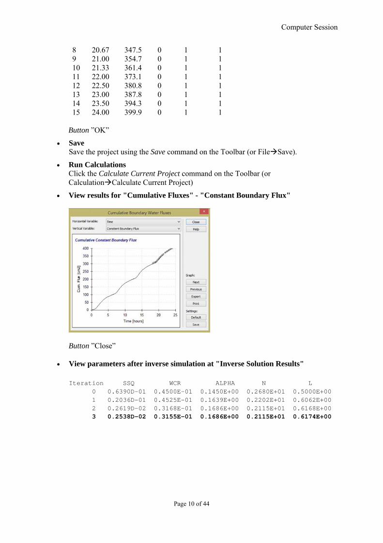
Inverse Solution Data (EditFlow and Transport ParametersData for Inverse Solution) Assumption: 4th loading will be used for comparing simulation results with measured data i.e. Inverse Solution Data table (Table 1): X-column: time + 18 hours, Y-column: + 300 cm² (1 single loading: 100 cm²) one single loading = 10 mm = 10 L/m² = 10 * 1000 cm³ / 100 cm = 100 cm² Inverse Solution Data table:

X Y Type Position Weight 1 18.33 303.1 0 1 1 2 18.67 306.4 0 1 1 3 19.00 309.9 0 1 1 4 19.33 314.9 0 1 1 5 19.67 323.6 0 1 1 6 20.00 331.4 0 1 1 7 20.33 339.5 0 1 1

Computer Session

of 44

8 20.67 347.5 0 1 1 9 21.00 354.7 0 1 1 10 21.33 361.4 0 1 1 11 22.00 373.1 0 1 1 12 22.50 380.8 0 1 1 13 23.00 387.8 0 1 1 14 23.50 394.3 0 1 1 15 24.00 399.9 0 1 1

Button ”OK”


Run Calculations Click the Calculate Current Project command on the Toolbar (or CalculationCalculate Current Project)

View results for "Cumulative Fluxes" - "Constant Boundary Flux"

Button ”Close”

View parameters after inverse simulation at "Inverse Solution Results" Iteration SSQ WCR ALPHA N L 0 0.6390D-01 0.4500E-01 0.1450E+00 0.2680E+01 0.5000E+00 1 0.2036D-01 0.4525E-01 0.1639E+00 0.2202E+01 0.6062E+00 2 0.2619D-02 0.3168E-01 0.1686E+00 0.2115E+01 0.6168E+00 3 0.2538D-02 0.3155E-01 0.1686E+00 0.2115E+01 0.6174E+00

Computer Session

of 44

Simulation 4 - Update Steady-State Water Flow Results 1:

Project Manager (FileProject Manager) Select "Example 1b" Button ”Copy” Enter New Name: Example 1d Description: VF wetland - flow simulation - update steady-state flow Button ”OK” Button ”Open” Example 1d

Water Flow - Soil-Hydraulic Params (EditFlow and Transport ParametersWater Flow ParametersSoil Hydraulic Parameters) Change parameters to estimated values, i.e. Qr = 0.032, Alpha = 0.169, n = 2.11 and l = 0.617 Button ”OK”



Results – Other Information: Boundary Fluxes (from the Navigator Bar, or ResultsBoundary InformationBoundary Fluxes) Select "Constant Boundary Flux" - notice that initially there was not steady state Button ”Close”


Computer Session

of 44

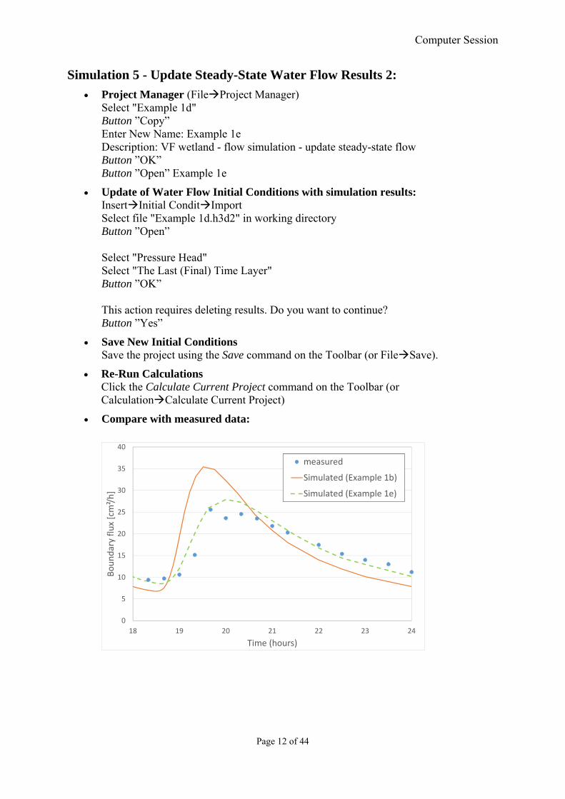
Simulation 5 - Update Steady-State Water Flow Results 2:

Project Manager (FileProject Manager) Select "Example 1d" Button ”Copy” Enter New Name: Example 1e Description: VF wetland - flow simulation - update steady-state flow Button ”OK” Button ”Open” Example 1e

Update of Water Flow Initial Conditions with simulation results: InsertInitial ConditImport Select file "Example 1d.h3d2" in working directory Button ”Open” Select "Pressure Head" Select "The Last (Final) Time Layer" Button ”OK” This action requires deleting results. Do you want to continue? Button ”Yes”

Save New Initial Conditions Save the project using the Save command on the Toolbar (or FileSave).

Re-Run Calculations Click the Calculate Current Project command on the Toolbar (or CalculationCalculate Current Project)

Compare with measured data:

0

5

10

15

20

25

30

35

40

18 19 20 21 22 23 24

Boundary flux [cm²/h]

Time (hours)

measured

Simulated (Example 1b)

Simulated (Example 1e)

Computer Session

of 44

2 Reactive Transport in a Vertical Flow Wetland (CW2D Biokinetic Model)

This example demonstrate the set-up of a project with reactive transport in a vertical flow wetland (VF wetland) using the CW2D biokinetic model.


The VF wetland is the same as in Example 1. The calibrated flow model will be used to set-up a reactive transport simulation using the CW2D biokinetic model. Table 2 shows the CW2D influent concentrations.

Table 2. CW2D influent concentrations (as used in "Wetland 1", Langergraber and Šimůnek, 2006)

Component SO CR CS CI XH XANs XANb NH4N NO2N NO3N N2 PO4PConcentration 1 160 120 20 0 0 0 60 0.1 0.1 0 10



Project Manager (FileProject Manager) Select: Example 1e Button ”Copy” Name: Example 2a Description: VF wetland - reactive transport simulation (CW2D) Button ”OK”

Open project "Example 2a" Select: Example 2a Button ”Open”

Main Processes (EditFlow and Transport ParametersMain Processes) Check Box: Water Flow Check Box: Solute Transport Check the Radio Button: Wetland (the CW2D module should be selected by default) Button ”Next” Delete Results: "OK"

Time Information (EditFlow and Transport ParametersTime Information) Final Time: 48 (simulation over 2 days) Maximum Time Step: 1 Number of times to repeat the same set of BC records: 2 Button ”OK”

Output Information (EditFlow and Transport ParametersOutput Information) Print Options: Check T-Level Information Every n time step: 1 Print Times: Button ”Default” Button ”OK”

Computer Session

of 44

Solute Transport – General Info (EditFlow and Transport ParametersSolute Transport ParametersGeneral Information ) Set "Mass units" = µg Button ”Next”

Solute Transport – Transport Parameters (EditFlow and Transport ParametersSolute Transport Parameters Solute Transport Parameters) Soil specific parameters Set parameter "Fract." = 0 (mandatory for the Wetland module) Solute specific parameters (in cm²/h):

Sol Diffus.W. Diffus.G.1 0.072 769 2 0.0456 0 3 0.0456 0 4 0.0456 0 5 0 0 6 0 0 7 0 0 8 0.0801 0 9 0.0801 0 10 0.0801 0 11 0.0801 0 12 0.0801 0 13 0. 0

Button ”OK”

Solute Transport – Reaction Parameters (EditFlow and Transport ParametersSolute Transport Parameters Solute Reaction Parameters) Leave default parameters and browse through all these windows Button ”Next”

Solute Transport – Constructed Wetland Model (CW2D) Parameters I (EditFlow and Transport ParametersSolute Transport Parameters Constructed Wetland Parameters I) Explore and leave default parameters Button ”Next”

Solute Transport – Constructed Wetland Model (CW2D) Parameters II (EditFlow and Transport ParametersSolute Transport Parameters Constructed Wetland Parameters II) Explore and leave default parameters Button ”Next”

Time-Variable Boundary Conditions (EditFlow and Transport ParametersVariably Boundary Conditions) add influent concentrations: cVal1-1 = 1 cVal1-2 = 160 cVal1-3 = 120

Computer Session

of 44

cVal1-4 = 20 cVal1-8 = 60 cVal1-9 = 0.1 cVal1-10 = 0.1 cVal1-12 = 10 Copy values to all lines

Solute Transport Initial Conditions: Navigator Bar click on Initial Conditions – L1 – Dissolved Oxygen Select the entire transport domain and click on the Set L1 - IC Dissolved Oxygen command at the Edit Bar, check Use top value for entire selected region, check that Top value is set equal 1. Button ”OK” Repeat for L2, L3, L4, L8, L9, L10, L12, S5, S6, S7 Note: it is assumed that a clean sand is used and that the filter has not been loaded previously. Steady-state conditions for reactive transport are reached once the biomass has reached constant concentrations, which can be expected after longer simulation time (e.g. ,100 days).

Solute Transport Boundary Conditions: Navigator Bar click on Boundary Conditions – Solute Transport Select Third-type Boundary from the Edit Bar, and select the top of the boundary. Pointer to the vector of the boundary Conditions = 1 Button ”OK”

Domain Properties - Observation Nodes: Insert Observation Nodes

Computer Session

of 44



Results – Other Information: Observation Points (from the Navigator Bar) Select "Observation Points " View results, 1st: check oxygen concentrations Vertical Variable: select "L1 – Dissolved Oxygen

Note that L1 (Dissolved Oxygen) concentrations at the upper Observation Nodes (Nos.1-4) show numerical oscillations. The reason is that, oxygen consumption is by far the fastest process among all the reactions considered. Too avoid these numerical oscillations the maximum time step needs to be reduced.

Advice: L1 (Dissolved Oxygen) concentrations should always be checked prior to other concentrations to avoid numerical instabilities.

Computer Session

of 44


Project Manager (FileProject Manager) Select: Example 2a Button ”Copy” Name: Example 2b Description: VF wetland - reactive transport simulation (CW2D) – reduced dt Button ”OK”

Open project "Example 2b" Select: Example 2b Button ”Open”

Time Information (EditFlow and Transport ParametersTime Information) Maximum Time Step: 0.02 Button ”OK”



Results – Other Information: Observation Points (from the Navigator Bar) Select " Observation Points " View results, 1st: check oxygen concentrations Vertical Variable: select "L1 – Dissolved Oxygen

Note that L1 (Dissolved Oxygen) concentrations do not show numerical oscillations anymore the maximum time step used is OK.

Computer Session

of 44

Check the other results: e.g. Growth of heterotrophic bacteria Vertical Variable: select "S5 – Heterotr. Micro."

e.g. Growth of ammonia oxidisers Vertical Variable: select "S6 – Autotr. Micro - NS"

Button ”Close”


Computer Session

of 44

3 Water Flow and Reactive Transport in a Horizontal Flow Wetland (CWM1 Biokinetic Model)

This example demonstrates the set-up of a water flow and reactive transport simulation in a horizontal flow (HF) wetland using the CWM1 biokinetic model.

The example consists of the following three steps:

1. Project set up, a 24-h long simulation to reach steady-state conditions for water flow. 2. Simulation of a tracer experiment.

a. Set-up of tracer simulation b. Inverse simulation to match measured data c. Updated tracer simulation

3. Simulation of reactive transport (CWM1 biokinetic model). 4. Simulation of reactive transport (CWM1 biokinetic model) and effects of wetland

plants.


The HF bed as described by Langergraber and Šimůnek (2012) is used in this example. The HF bed has a length of 10.3 m, a depth of 0.55 m and a width of 5.3 m. The water level in the bed is 0.5 m. The gravel of the main layer has d60 of 10 mm and porosity of 41 %.

The first 0.3 m of the bed, the mixing zone, is filled with course gravel (porosity 45 %). The HYDRUS implementation considers the mixing zone (a red circle in Figure 1, that also shows a typical flow path in a HF bed).

Figure 1: Implementation of the HF bed.

In the HYDRUS implementation, the vertical domain of 10.3 m and 0.6 m was discretized into 33 columns and 23 rows, resulting in a two-dimensional finite element mesh consisting of 805 nodes and 1496 triangular finite elements. An atmospheric boundary condition was applied at the top of the mixing zone, whereas the effluent boundary was represented using a constant head boundary condition (0.5 m) at the bottom of the right end of the bed

The HF bed was loaded with wastewater with a hydraulic loading rate of 36 mm.d-1.

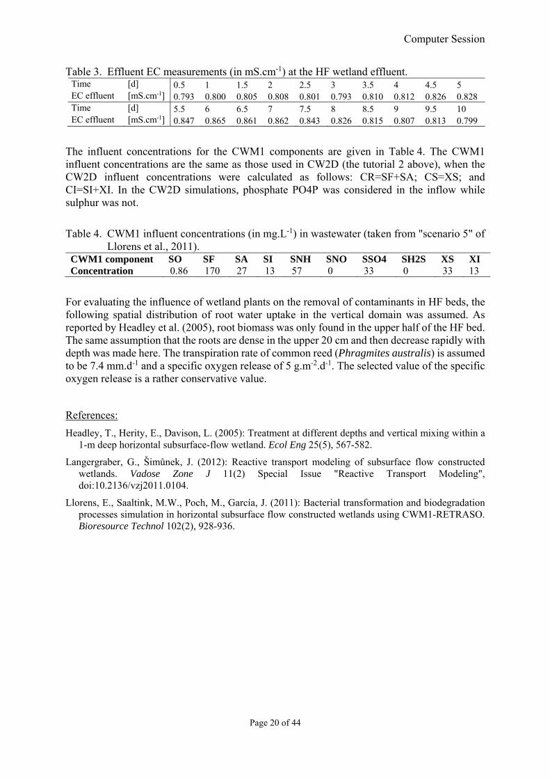
To characterize the hydraulic behavior, a tracer experiment with KCl was carried out. The tracer concentration was measured by measuring the electrical conductivity (EC) in the influent and effluent of the HF wetland. A KCl solution with EC of 30 mS.cm-1 was added for a duration of 10 minutes and then the tracer breakthrough curve was measured at the effluent of the HF wetland. During the tracer experiment the background EC was 0.8 mS.cm-1. Table 3 shows measured effluent EC during a period of 10 days.

Computer Session

of 44

Table 3. Effluent EC measurements (in mS.cm-1) at the HF wetland effluent. Time [d] 0.5 1 1.5 2 2.5 3 3.5 4 4.5 5 EC effluent [mS.cm-1] 0.793 0.800 0.805 0.808 0.801 0.793 0.810 0.812 0.826 0.828 Time [d] 5.5 6 6.5 7 7.5 8 8.5 9 9.5 10 EC effluent [mS.cm-1] 0.847 0.865 0.861 0.862 0.843 0.826 0.815 0.807 0.813 0.799

The influent concentrations for the CWM1 components are given in Table 4. The CWM1 influent concentrations are the same as those used in CW2D (the tutorial 2 above), when the CW2D influent concentrations were calculated as follows: CR=SF+SA; CS=XS; and CI=SI+XI. In the CW2D simulations, phosphate PO4P was considered in the inflow while sulphur was not.

Table 4. CWM1 influent concentrations (in mg.L-1) in wastewater (taken from "scenario 5" of

Llorens et al., 2011). CWM1 component SO SF SA SI SNH SNO SSO4 SH2S XS XIConcentration 0.86 170 27 13 57 0 33 0 33 13

For evaluating the influence of wetland plants on the removal of contaminants in HF beds, the following spatial distribution of root water uptake in the vertical domain was assumed. As reported by Headley et al. (2005), root biomass was only found in the upper half of the HF bed. The same assumption that the roots are dense in the upper 20 cm and then decrease rapidly with depth was made here. The transpiration rate of common reed (Phragmites australis) is assumed to be 7.4 mm.d-1 and a specific oxygen release of 5 g.m-2.d-1. The selected value of the specific oxygen release is a rather conservative value.

References:

Headley, T., Herity, E., Davison, L. (2005): Treatment at different depths and vertical mixing within a 1-m deep horizontal subsurface-flow wetland. Ecol Eng 25(5), 567-582.

Langergraber, G., Šimůnek, J. (2012): Reactive transport modeling of subsurface flow constructed wetlands. Vadose Zone J 11(2) Special Issue "Reactive Transport Modeling", doi:10.2136/vzj2011.0104.

Llorens, E., Saaltink, M.W., Poch, M., García, J. (2011): Bacterial transformation and biodegradation processes simulation in horizontal subsurface flow constructed wetlands using CWM1-RETRASO. Bioresource Technol 102(2), 928-936.

Computer Session

of 44



Project Manager (FileProject Manager) Button ”New”

New Project (or FileNew Project) Name: Example 3a Description: HF wetland - flow simulation Working Directory: Temporary – is deleted after closing the project Button ”Next”

Domain Type and Units (EditDomain GeometryDomain Type and Units) Type of Geometry: 2D - Simple 2D-Domain Options: 2D - Vertical Plane XZ Units: m Initial Workspace: Xmin=0 m, Xmax=12 m, Zmin=0 m, Zmax=2 m Check "Set View Stretching Factors Automatically" Button ”Next”

Rectangular Domain Definition (EditDomain GeometrySimple Domain) Lx = 10.3 m, Lz = 0.55 m, = 0° Button ”Next”

Main Processes (EditFlow and Transport ParametersMain Processes) Check Box: Water Flow Button ”Next”

Time Information (EditFlow and Transport ParametersTime Information) Time Units: hours Final Time: 24 Initial Time Step: 0.001 Minimum Time Step: 0.0001 Maximum Time Step: 1 Check "Time-Variable Boundary Conditions" Number of Time-Variable Boundary Records: 1 Number of times to repeat the same set of BC records: 1 Button ”Next”

Output Information (EditFlow and Transport ParametersOutput Information) Print Options: Check T-Level Information Check Screen Output Check Press Enter at the End Print Times: Count: 12 Update Number of Subregions: 1 Button ”Next”

Water Flow - Iteration Criteria (EditFlow and Transport ParametersWater Flow ParametersIteration Criteria ) Leave default values Button ”Next”

Computer Session

of 44

Water Flow – Soil-Hydraulic Model (EditFlow and Transport ParametersWater Flow ParametersHydraulic Properties Model) Radio button - van Genuchten-Mualem Radio button - No hysteresis Button ”Next”

Water Flow - Soil-Hydraulic Params (EditFlow and Transport ParametersWater Flow ParametersSoil Hydraulic Parameters) Number of Materials: 2 Button "Update" Material 1 (gravel of main layer): Select "Sand" from Soil Catalog Enter values for Qs = 0.41; n = 4 and Ks = 10 m/h Name: Gravel (Main Layer) Material 2 (course gravel in mixing zone): Select "Sand" from Soil Catalogue Enter values for Qs = 0.45; n = 4 and Ks = 50 m/h Name: Gravel (Mixing Zone) Button ”Next”

Time-Variable Boundary Conditions (EditFlow and Transport ParametersVariably Boundary Conditions) Calculations: hydraulic loading rate = 36 mm.d-1 = 1.5 mm.h-1 = 1.5 L.m-2.h-1 surface area of whole HF bed: 10.3 m x 5.3 m = 54.6 m² hydraulic loading (whole bed) = 1.5 L.m-2.h-1 x 54.6 m² = 81.9 L.h-1 = 0.0819 m³.h-1 surface area of mixing zone = 0.3 m x 5.3 m = 1.6 m² hydraulic loading rate (mixing zone) = 0.082 m³.h-1 / 1.6 m² = 0.051 m.h-1 Time-Variable Boundary Conditions: Time Precip. Evap. Transp. hCritA

[hours] [m/h] [m/h] [m/h] [m]

1 24 0.051 0 0 100 Remaining columns = 0

Button ”Next”

Computer Session

of 44

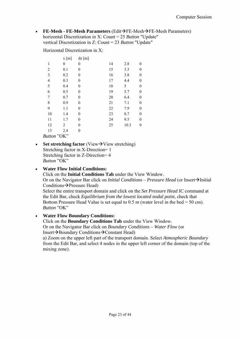
FE-Mesh - FE-Mesh Parameters (EditFE-MeshFE-Mesh Parameters) horizontal Discretization in X: Count = 25 Button "Update" vertical Discretization in Z: Count = 23 Button "Update"

Horizontal Discretization in X:

x [m] dz [m] 1 0 0 14 2.8 0 2 0.1 0 15 3.3 0 3 0.2 0 16 3.8 0 4 0.3 0 17 4.4 0 5 0.4 0 18 5 0 6 0.5 0 19 5.7 0 7 0.7 0 20 6.4 0 8 0.9 0 21 7.1 0 9 1.1 0 22 7.9 0 10 1.4 0 23 8.7 0 11 1.7 0 24 9.5 0 12 2 0 25 10.3 0 13 2.4 0

Button ”OK”

Set stretching factor (ViewView stretching) Stretching factor in X-Direction= 1 Stretching factor in Z-Direction= 4 Button ”OK”

Water Flow Initial Conditions: Click on the Initial Conditions Tab under the View Window. Or on the Navigator Bar click on Initial Conditions – Pressure Head (or InsertInitial ConditionsPressure Head) Select the entire transport domain and click on the Set Pressure Head IC command at the Edit Bar, check Equilibrium from the lowest located nodal point, check that Bottom Pressure Head Value is set equal to 0.5 m (water level in the bed = 50 cm). Button ”OK”

Water Flow Boundary Conditions: Click on the Boundary Conditions Tab under the View Window. Or on the Navigator Bar click on Boundary Conditions – Water Flow (or InsertBoundary ConditionsConstant Head) a) Zoom on the upper left part of the transport domain. Select Atmospheric Boundary from the Edit Bar, and select 4 nodes in the upper left corner of the domain (top of the mixing zone).

Computer Session

of 44

b) Zoom on the lower right part of the transport domain. Select Constant Head from the Edit Bar, select 1 node at the lower right boundary (outlet of the HF bed)

Specify Constant Pressure Head Value: 0.475 m

Computer Session

of 44

Material Distribution: Click on the Domain Properties Tab under the View Window. Or on the Navigator Bar click on Domain Properties – Material Distribution (or InsertDomain Properties Material Distribution) Zoom on the left part of the transport domain. Click the "Gravel (Mixing Zone)" and select the first 3 columns on left side to assign the mixing zone.

Observation Nodes: Click on the Domain Properties Tab under the View Window. Or on the Navigator Bar click on Domain Properties – Observation Nodes (or InsertDomain PropertiesObservation Nodes) Click the "Insert Observation Node" command on the Edit Bar and insert 6 observation nodes along the flow path. 1 observation node should be located at the effluent node.

Computer Session

of 44



Results – Graphical Display: Pressure Head (from the Navigator Bar, or ResultsDisplay Quantity Pressure Head) View results at end of simulation time, i.e. 24 hours

Computer Session

of 44

View also results for velocity vectors.


Update of Water Flow Initial Conditions with simulation results from before: InsertInitial ConditImport Select file "Example 3a.h3d2" in the project directory Button ”Open” Select "Pressure Head" Select "The Last (Final) Time Layer" Button ”OK” Warning: This action requires deleting results. Do you want to continue? Button ”Yes”




Computer Session

of 44

Simulation 2a – Set-up Tracer Simulation

Project Manager (FileProject Manager) Select "Example 3a" Button ”Copy” Enter New Name: Example 3b1 Description: HF wetland – tracer simulation Button ”OK” Button ”Open” Example 3b1

Main Processes (EditFlow and Transport ParametersMain Processes) Check Box: Water Flow Check Box: Solute Transport Check Radio Button "Standard Solute Transport" Button ”Next”

Time Information (EditFlow and Transport ParametersTime Information) Time Units: Check Radio Button ”Days” Final Time: 10 Boundary Conditions: Number of Time-Variably Boundary Conditions: 2 Button ”Next”

Output Information (EditFlow and Transport ParametersOutput Information) Print Times: Count: 40 (output every 6 hours = 0.25 days) Button ”Update” Button ”Default” Button ”OK”

Solute Transport – General Info (EditFlow and Transport ParametersSolute Transport ParametersGeneral Information…) Set "Mass units" = g Button ”Next”

Solute Transport – Transport Parameters (EditFlow and Transport ParametersSolute Transport Parameters Solute Transport Parameters…) Leave default values. Button ”OK”

Time-Variable Boundary Conditions (EditFlow and Transport ParametersVariably Boundary Conditions)

Time Precip. Evap. … cValue 1 cValue 2 cValue 3 [days] [m/day] [m/day] g/L^3 g/L^3 g/L^3 0.00694 1.224 0 … 30 0 0 10 1.2246 0 … 0.8 0 0

KCl solution with EC 30 mS/cm-1 is added for 10 min (= 0.00694 days), afterward influent concentration is background EC of 0.8 mS/cm-1.

Button ”OK”

Computer Session

of 44

Solute Transport Initial Conditions: Navigator Bar click on Initial Conditions – Concentration Select the entire transport domain and click on the Set Concentration IC command at the Edit Bar, check Use top value for entire selected region, check that Top value is set equal 0.8. Button ”OK”

Solute Transport Boundary Conditions: Select Third-type Boundary from the Edit Bar, and nodes from mixing zone selected as Atmospheric BC. Pointer to the vector of the boundary Conditions = 1 (note that this was already the default value). Button ”OK”



Results – Other Information – Observation points – Concentration

Computer Session

of 44

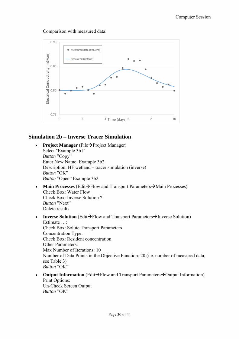
Comparison with measured data:

Simulation 2b – Inverse Tracer Simulation

Project Manager (FileProject Manager) Select "Example 3b1" Button ”Copy” Enter New Name: Example 3b2 Description: HF wetland – tracer simulation (inverse) Button ”OK” Button ”Open” Example 3b2

Main Processes (EditFlow and Transport ParametersMain Processes) Check Box: Water Flow Check Box: Inverse Solution ? Button ”Next” Delete results

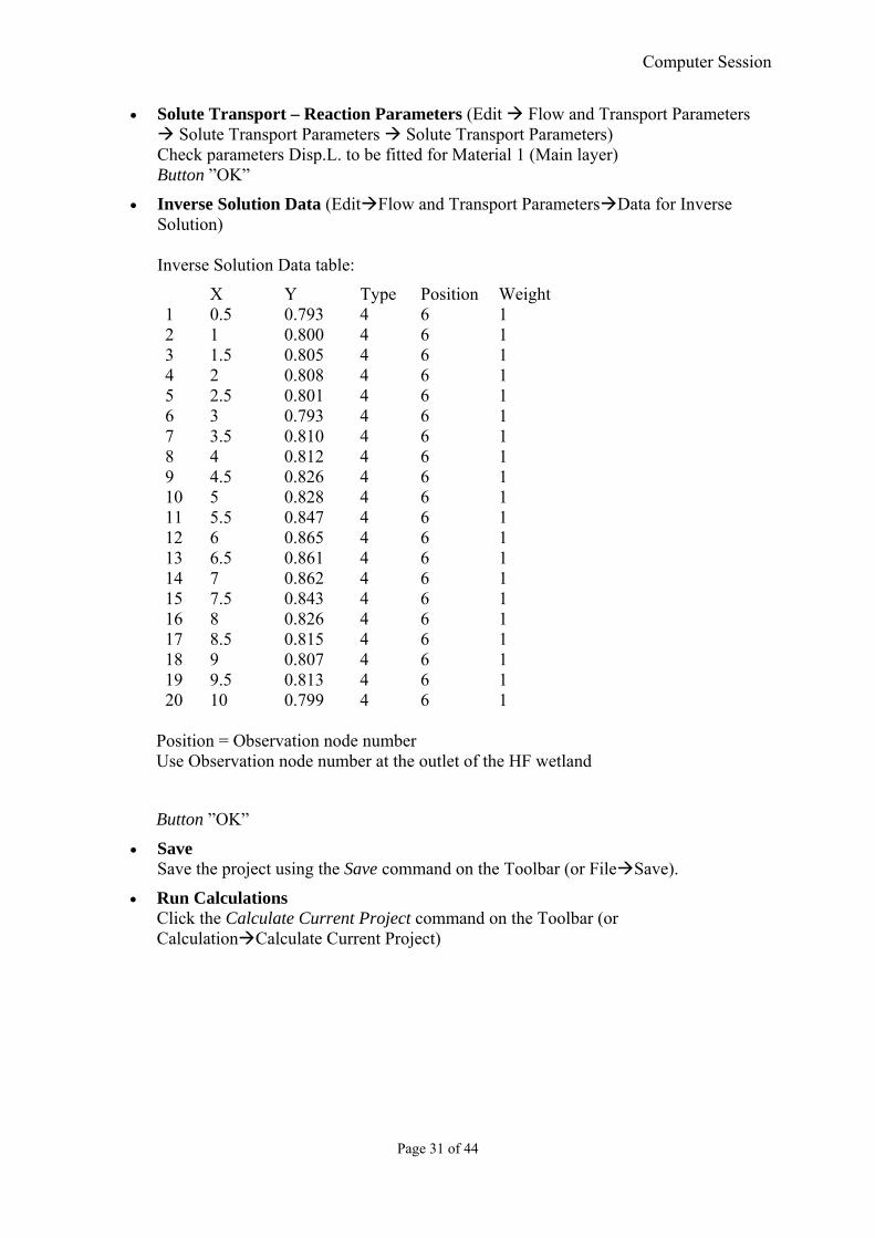
Inverse Solution (EditFlow and Transport ParametersInverse Solution) Estimate …: Check Box: Solute Transport Parameters Concentration Type: Check Box: Resident concentration Other Parameters: Max Number of Iterations: 10 Number of Data Points in the Objective Function: 20 (i.e. number of measured data, see Table 3) Button ”OK”

Output Information (EditFlow and Transport ParametersOutput Information) Print Options: Un-Check Screen Output Button ”OK”

0.75

0.80

0.85

0.90

0 2 4 6 8 10

Electrical Conductivity [m

S/cm

]

Time (days)

Measured data (effluent)

Simulated (default)

Computer Session

of 44

Solute Transport – Reaction Parameters (Edit Flow and Transport Parameters Solute Transport Parameters Solute Transport Parameters) Check parameters Disp.L. to be fitted for Material 1 (Main layer) Button ”OK”

Inverse Solution Data (EditFlow and Transport ParametersData for Inverse Solution) Inverse Solution Data table:

X Y Type Position Weight 1 0.5 0.793 4 6 1 2 1 0.800 4 6 1 3 1.5 0.805 4 6 1 4 2 0.808 4 6 1 5 2.5 0.801 4 6 1 6 3 0.793 4 6 1 7 3.5 0.810 4 6 1 8 4 0.812 4 6 1 9 4.5 0.826 4 6 1 10 5 0.828 4 6 1 11 5.5 0.847 4 6 1 12 6 0.865 4 6 1 13 6.5 0.861 4 6 1 14 7 0.862 4 6 1 15 7.5 0.843 4 6 1 16 8 0.826 4 6 1 17 8.5 0.815 4 6 1 18 9 0.807 4 6 1 19 9.5 0.813 4 6 1 20 10 0.799 4 6 1

Position = Observation node number Use Observation node number at the outlet of the HF wetland

Button ”OK”



Computer Session

of 44

Results – Other Information – Observation points – Concentration

Button ”Close”

View parameters after inverse simulation at "Inverse Solution Results" Iteration SSQ DISPL 0 0.2382D+00 0.5000E+00 1 0.8620D-01 0.2765E+00 2 0.5771D-01 0.1789E+00 3 0.5659D-01 0.1912E+00 4 0.5658D-01 0.1917E+00

Computer Session

of 44

Simulation 2c – Updated Tracer Simulation

Project Manager (FileProject Manager) Select "Example 3b1" Button ”Copy” Enter New Name: Example 3b3 Description: HF wetland – tracer simulation (updated) Button ”OK” Button ”Open” Example 3b3

Solute Transport – Transport Parameters (EditFlow and Transport ParametersSolute Transport Parameters Solute Transport Parameters…) Material 1: Disp.L. = 0.192 m Button ”OK”



Results Comparison with measured data:

0.75

0.80

0.85

0.90

0 2 4 6 8 10

Electrical Conductivity [m

S/cm

]

Time (days)

Measured data (effluent)

Simulated (default)

Simulated (fitted)

Computer Session

of 44

Simulation 3 – Set-up Reactive Transport Simulations

Project Manager (FileProject Manager) Select "Example 3a" Button ”Copy” Enter New Name: Example 3c Description: HF wetland – reactive transport simulation (CWM1) Button ”OK” Button ”Open” Example 3c

Main Processes (EditFlow and Transport ParametersMain Processes) Check Box: Water Flow Check Box: Solute Transport Check Radio Buttons "Wetland module" and "CWM1" Button ”Next”

Time Information (EditFlow and Transport ParametersTime Information) Final Time: 48 (simulation over 2 days) Maximum Time Step: 0.01 (has to be reduced due to fast oxygen consumption) Button ” Next”

Output Information (EditFlow and Transport ParametersOutput Information) Print Options: Check T-Level information; Every n time step: 10 Print Times: Count: 24 Button ”Update” Button ”Default” Button ”OK”

Solute Transport – General Info (EditFlow and Transport ParametersSolute Transport ParametersGeneral Information ) Set "Mass units" = g Button ”Next”

Solute Transport – Transport Parameters (EditFlow and Transport ParametersSolute Transport Parameters Solute Transport Parameters) Soil specific parameters Set parameter "Fract." = 0 for both materials

Computer Session

of 44

Solute specific parameters (in m²/h): Sol Diffus.W. Diffus.G.1 7.21e-6 0.0769 2 4.56e-6 0 3 4.56e-6 0 4 4.56e-6 0 5 8.01e-6 0 6 8.01e-6 0 7 8.01e-6 0 8 8.01e-6 0 9 4.56e-6 0 10 4.56e-6 0 11 0 0 12 0 0 13 0 0 14 0 0 15 0 0 16 0 0 17 0 0

Button ”Next”

Solute Transport – Reaction Parameters (EditFlow and Transport ParametersSolute Transport Parameters Solute Reaction Parameters) Leave default parameters and browse through all these windows Button ”Next”

Solute Transport – Constructed Wetland Model (CWM1) Parameters I (EditFlow and Transport ParametersSolute Transport Parameters Constructed Wetland Parameters I) Explore and leave default parameters Button ”Next”

Solute Transport – Constructed Wetland Model (CWM1) Parameters II (EditFlow and Transport ParametersSolute Transport Parameters Constructed Wetland Parameters II) Explore and leave default parameters Button ”Next”

Time-Variable Boundary Conditions (EditFlow and Transport ParametersVariably Boundary Conditions) Change Time to 48 hours add influent concentrations: cVal1-1 = 0.86 cVal1-2 = 170 cVal1-3 = 27 cVal1-4 = 13 cVal1-5 = 57 cVal1-7 = 33 cVal1-9 = 33 cVal1-10 = 13

Computer Session

of 44

Button ”OK”

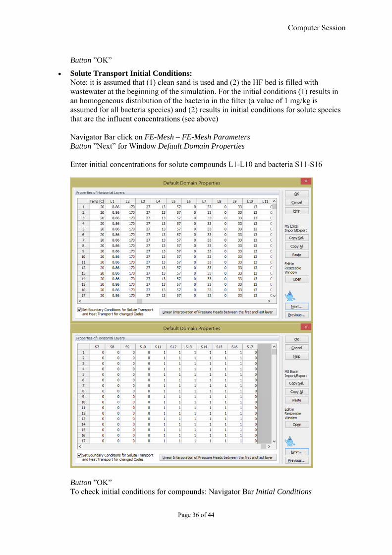
Solute Transport Initial Conditions: Note: it is assumed that (1) clean sand is used and (2) the HF bed is filled with wastewater at the beginning of the simulation. For the initial conditions (1) results in an homogeneous distribution of the bacteria in the filter (a value of 1 mg/kg is assumed for all bacteria species) and (2) results in initial conditions for solute species that are the influent concentrations (see above) Navigator Bar click on FE-Mesh – FE-Mesh Parameters Button ”Next” for Window Default Domain Properties Enter initial concentrations for solute compounds L1-L10 and bacteria S11-S16

Button ”OK” To check initial conditions for compounds: Navigator Bar Initial Conditions

Computer Session

of 44

Solute Transport Boundary Conditions: Navigator Bar click on Boundary Conditions – Solute Transport Select Third-type Boundary from the Edit Bar, and nodes from mixing zone selected as Atmospheric BC. Pointer to the vector of the boundary Conditions = 1 (note that this was already the default value). Button ”OK”



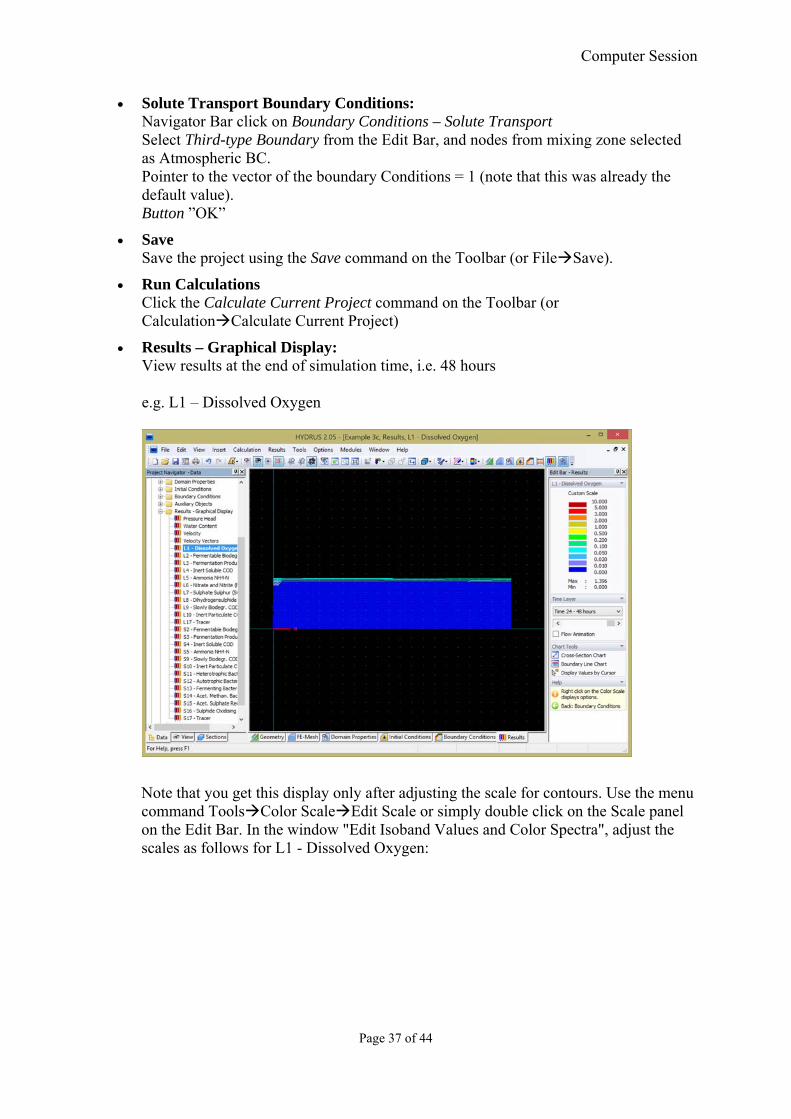
Results – Graphical Display: View results at the end of simulation time, i.e. 48 hours e.g. L1 – Dissolved Oxygen

Note that you get this display only after adjusting the scale for contours. Use the menu command ToolsColor ScaleEdit Scale or simply double click on the Scale panel on the Edit Bar. In the window "Edit Isoband Values and Color Spectra", adjust the scales as follows for L1 - Dissolved Oxygen:

Computer Session

of 44

and for S11 – Heterotrophic Bacteria

The definition of the scale can be saved for future use using the command "Copy..". The scale can be saved under various names, such as "Dissolved Oxygen" or "Heterotrophic Bacteria".

Computer Session

of 44

Results – Other Information: Observation Points (from the Navigator Bar) check simulation results at observation points, e.g., select L2 and L3

Button ”Close”


Note: Usually simulations need to be run until steady-state is reached, i.e. the patterns of the bacteria concentrations obtained do not change anymore.

Computer Session

of 44

Simulation 4 – Set-up Simulation that Considers Wetland Plants

Project Manager (FileProject Manager) Select "Example 3c" Button ”Copy” Enter New Name: Example 3d Description: HF wetland – reactive transport simulation (CWM1) + plants Button ”OK” Button ”Open” Example 3d

Update of Water Flow Initial Conditions with simulation results from before: InsertInitial ConditionImport Select file "Example 3b.h3d2" in working directory Button ”Open” Button "Select All" Select "The Last (Final) Time Layer" Button ”OK” Warning: This action requires deleting results. Do you want to continue? Button ”Yes”


Main Processes (EditFlow and Transport ParametersMain Processes) Check Box: Water Flow Check Box: Solute Transport Check Box: Root Water Uptake Button ”OK”

Root Water and Solute Uptake: Models (EditFlow and Transport Parameters Root Water and Solute Uptake Root Water/Solute Uptake Models) Water Uptake Reduction Model: S-Shaped Solute Stress Model: No Solute Stress Button ”Next”

Root Water and Solute Uptake: Root Water Uptake Parameters (EditFlow and Transport Parameters Root Water and Solute Uptake Pressure Head Reduction) P50 [m] = -1; P3 [-] = 3; PW [m] = -100; Button ”OK”

Solute Transport – Reaction Parameters (EditFlow and Transport ParametersSolute Transport Parameters Solute Reaction Parameters) L1 (Dissolved Oxygen): cRoot = -675 L5 (Ammonia NH4): cRoot = 50 L6 (Nitrate NO3): cRoot = 50 Button ”OK”

Time-Variable Boundary Conditions (EditFlow and Transport ParametersVariably Boundary Conditions) Calculation: Transpiration = 7.4 L.m-2.d-1 = 7.4 mm.d-1 = 0.0074 m.d-1 = 0.00031 m.h-1

Computer Session

of 44

"Length of soil surface associated with transpiration" = 10 m. Button ”OK”

Root Distribution: Click on the Domain Properties Tab under the View Window. Or on the Navigator Bar click on Domain Properties – Root Water Uptake (or InsertDomain PropertiesRoot Distribution) (1) Click on "Properties in Table" on the Edit bar Enter the Root distribution as follows:

Note that this table displayes values that are constant for the entire horizontal layer (for all nodes on one horizontal line). It hides values that are different along the line. Button ”OK” (2) Zoon on the upper left part of the transport domain. Select the first 4 columns on the left side of the transport domain (mixing zone) Click on the "Set Root Water Uptake" on the Edit Bar: Top Value 0 Same value for all nodes "OK"

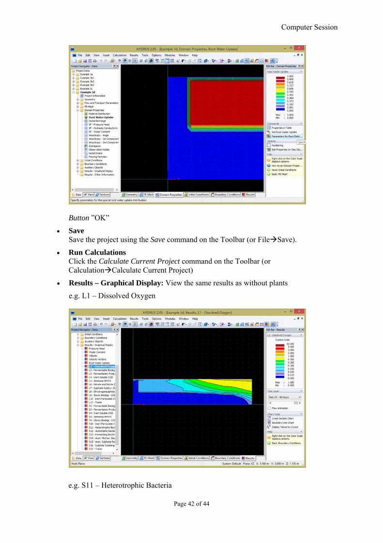
Computer Session

of 44

Button ”OK”



Results – Graphical Display: View the same results as without plants

e.g. L1 – Dissolved Oxygen

e.g. S11 – Heterotrophic Bacteria

Computer Session

of 44

Results – Other Information – Cumulative Fluxes: Select "Cumulative Actual Root Water Uptake"

Calculations:

Cumulative Root Water Uptake (in 2D) = 0.15 m* (in 48 hours)

Transpiration

… for the entire wetland surface: 0.15 m² x 5.3 m / 48h = 16.56 L.h-1

… for unit surface area: 16.56 L.h-1 x 24 h/d /(5.3*10 m²) = 7.5 L.m-2.d-1

Computer Session

of 44

Results – Other Information – Solute Fluxes: Select "Concentration number 1 (Dissolved Oxygen) Select "Cumulative Root Solute Uptake" Note: the minus sign denotes oxygen release

Calculations:

Oxygen Release = -100 g/m (in 48 hours)

… for the entire wetland surface: 100 g/m x 5.3 m(width) / 48h = -11.04 g.h-1

… for unit surface area: 11.04 g.h-1 x 24 h/d /(5.3*10 m²) = -5 g.m-2.d-1

Same calculations for:

L5 (Ammonium N): Root uptake = 7.43 g/m (in 48 hours) 0.37 g.m-2.d-1 L6 (Nitrate N): Root uptake = 0.0105 g/m (in 48 hours) 0.0005 g.m-2.d-1


tutorials for the hydrus wetland module - pc-progress · tutorials for the hydrus wetland module...

Documents