tvem (time‐varying effect modeling) sas macro users’ guide · pdf file%tvem sas macro...

TVEM (Time‐Varying Effect Modeling) SAS Macro Users’ Guide Version 3.1.0

Runze Li Penn State John J. Dziak Penn State Xianming Tan University of North Carolina Liying Huang Penn State Aaron T. Wagner Penn State Jingyun Yang Rush University Medical Center

Copyright 2015, Penn State. All rights reserved.

Please send questions and comments to [email protected].

The suggested citation for this users' guide is Li, R., Dziak, J. D., Tan, X., Huang, L. Wagner, A. T., & Yang, J. (2015). TVEM (time-varying effect modeling) SAS macro users’ guide (Version 3.1.0). University Park: The Methodology Center, Penn State. Retrieved from http://methodology.psu.edu The development of the SAS %TVEM macro was supported by National Institute on Drug Abuse Grant P50 DA039838. The content is solely the responsibility of the authors and does not necessarily represent the official views of NIDA or the National Institutes of Health. The authors of this document would like to thank Deborah Kloska for her contributions and Stephanie Lanza, Sara Vasilenko, and Amanda Applegate for their helpful comments.

%TVEM SAS Macro Users’ Guide 2

TABLE OF CONTENTS

OVERVIEW OF THE %TVEM MACRO ........................................................................................... 3 Users’ guide overview ............................................................................................................................... 3 TVEM macro features ............................................................................................................................... 3

SYSTEM REQUIREMENTS ........................................................................................................... 5

TIME-VARYING EFFECT MODELS ................................................................................................ 6

USING THE %TVEM MACRO ...................................................................................................... 8 Preparation ................................................................................................................................................ 8 Syntax changes in version 3.x................................................................................................................... 8 Running the %TVEM macro and syntax definitions .................................................................................. 9 About spline basis: Should I use B-spline or P-spline? ........................................................................... 13 Selecting the proper number of knots ..................................................................................................... 13 Choosing how to model within-subject correlation .................................................................................. 14

OUTPUT ................................................................................................................................. 16 Text output............................................................................................................................................... 16 Plots ......................................................................................................................................................... 16 SAS datasets ........................................................................................................................................... 17 External file (optional) .............................................................................................................................. 20

DATA ANALYSIS EXAMPLES ...................................................................................................... 21 Data preparation: Adding an intercept, recoding, and adding a title ....................................................... 21 Example with a normal distribution ......................................................................................................... 22 Example with normal distribution using B-spline ..................................................................................... 23 Example with a time-varying covariate .................................................................................................... 24 Example with a logistic distribution ......................................................................................................... 25 Example with logistic outcome using B-spline ........................................................................................ 27

TECHNICAL DETAILS ON SPLINE BASES ..................................................................................... 28 B-spline basis .......................................................................................................................................... 28 Truncated power basis ............................................................................................................................ 30 Technical differences between using B-spline and P-spline ................................................................... 31 Technical details about random effects ................................................................................................... 31


Overview of the %TVEM Macro

Users’ guide overview

This users’ guide describes how to use the %TVEM macro. This SAS macro can be used to estimate

time-varying coefficient functions in time-varying effect modeling for intensive longitudinal data when

the outcome has a normal distribution, logistic distribution, or Poisson distribution. Intensive longitudinal

data refers to longitudinal data with more frequent measurements than traditional longitudinal data, in

which there are typically only a few widely spaced waves of data for each individual. Traditional analytic

methods assume that covariates have constant (i.e., non-time-varying) effects on a time-varying

outcome. These macros estimate the time-varying effects of the covariates.

This guide assumes you have a working knowledge of time-varying effect modeling (TVEM). Tan,

Shiyko, Li, Li, & Dierker (2012) provide an introduction to TVEM for audiences in psychological science.

TVEM macro features

The previous version of the Methodology Center’s TVEM software was a suite of multiple SAS files,

one for each kind of distribution that could be modeled. The new version is a single self-contained SAS

file that handles normal, logistic, or Poisson outcomes.

Key features of the previous and current macros:

Option to include multiple non-time-varying covariates

Option to include multiple time-varying covariates

Accommodation of different distributions (normal, logistic, or Poisson) measured over time

Option to employ a penalized truncated power spline basis instead of a B-spline basis function

(Spline bases are discussed in Section 4.4 and Chapter 7)

The zero-inflated Poisson (ZIP) outcome distribution has not been implemented in version 3.0, but it is

planned future development. To access version 2.1.1 of the %TVEM macro for ZIP outcomes, visit the

%TVEM macro download page.

Important changes from version 2.1.1

Ability to model within-subject correlation using random effects or a robust sandwich variance

estimator


Consolidation into a single macro for usability

Enhanced screen output for improved interpretability

Option to generate new output datasets

Improved plotting ability (Workaround for any SAS-Java-Windows compatibility issues)

Enhanced code readability. (See Section 4.2.)


System Requirements

The %TVEM macro requires

SAS version 9.2 or above

SAS/IML (to generate B-spline or truncated power spline basis functions)

SAS/STAT (to estimate linear mixed effects models using PROC GLIMMIX)

Note: SAS/IML and SAS/STAT are sold separately from the base SAS package, but most university

licenses include them.

The macro has not been extensively tested on versions of SAS for operating systems other than

Microsoft Windows, but may function there. One of the plotting options offered by the %TVEM macro

requires Java and the SAS SGRENDER procedure, but a simpler plotting option that requires only the

usual SAS GPLOT procedure is available.


Time‐Varying Effect Models

TVEMs are a natural extension of linear regression models. The fundamental difference is this: in linear

regression models, a single estimate of each covariate’s effect is provided, but in TVEMs the

coefficients can vary over time (Hastie & Tibshirani, 1993). Intensive longitudinal data are generally

collected to capture temporal changes in a process, so it is natural to expect that both the outcome and

the relationships between the covariates and the outcome might change over time. TVEMs are

designed to evaluate whether and how the effects of covariates change over time.

Suppose we observe intensive longitudinal data {( , , ), 1,2, … , , 1,2, … , , where is

individual ′s response variable measured at time , and =( , , … , )′ is a corresponding -

dimensional covariate vector. Traditional linear models are

(1)

where we can set in order to include an intercept, and is a random error term.

A TVEM is defined as

, (2)

where are unknown coefficient functions that are assumed to be smooth over time t.

TVEM thus allows the effects to change over time, which may be particularly useful in the analysis of

longitudinal data.

The generalized time-varying effect model

Traditional generalized linear model theory (McCullagh & Nelder, 1989) assumes that

, ⋯ ,, (3)

where , , … , ′, is called a linear predictor, and the function ∙ is called the link function,

which may vary from case to case. For example, we can let for continuous responses, let

log / 1 if the outcome is binary, and let log if we assume follows a

Poisson distribution. In Equation 1, all coefficients in are assumed to be constant over time. This

1 1= ,ij ij p ijp ijy x x

1 1ijx ij

1 1( ) ( )ij ij ij p ij ijp ijy t x t x

1( ), , ( )pt t

( )g a a


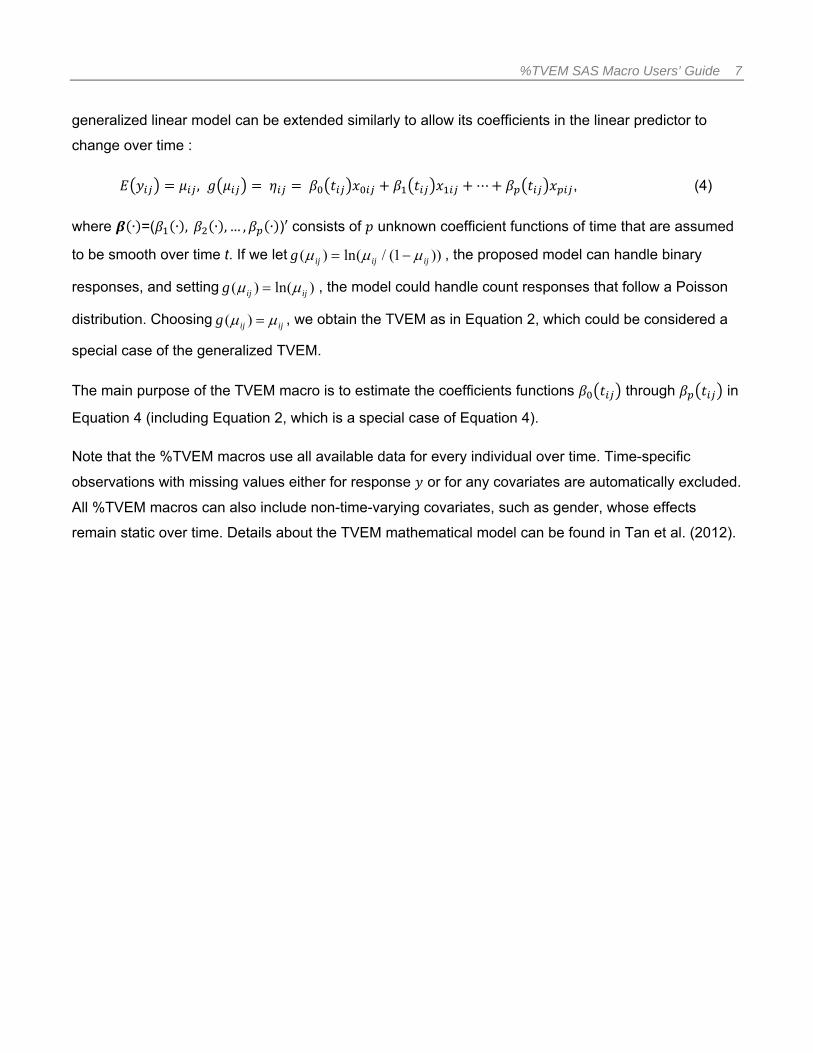
generalized linear model can be extended similarly to allow its coefficients in the linear predictor to

change over time :

, ⋯ , (4)

where ∙ =( ∙ , ∙ , … , ∙ )′ consists of unknown coefficient functions of time that are assumed

to be smooth over time t. If we let , the proposed model can handle binary

responses, and setting , the model could handle count responses that follow a Poisson

distribution. Choosing , we obtain the TVEM as in Equation 2, which could be considered a

special case of the generalized TVEM.

The main purpose of the TVEM macro is to estimate the coefficients functions through in

Equation 4 (including Equation 2, which is a special case of Equation 4).

Note that the %TVEM macros use all available data for every individual over time. Time-specific

observations with missing values either for response or for any covariates are automatically excluded.

All %TVEM macros can also include non-time-varying covariates, such as gender, whose effects

remain static over time. Details about the TVEM mathematical model can be found in Tan et al. (2012).

( ) ln( )/ (1 )ij ij ijg

( ) ln( )ij ijg

( )ij ijg


Using the %TVEM Macro

Preparation

A SAS macro is a special block of SAS commands. First the block is defined, and then it is called when

needed.

Three steps need to be completed before running one of the %TVEM macros:

If you haven’t already done so, download and save the macro to the designated path, (e.g.,

S:\myfolder\).

Direct SAS to read the macro code from the path, using a SAS %INCLUDE statement, such as

%INCLUDE ‘S:\myfolder\TVEM_v310.sas’;

Note: we suppose that the SAS macro file exists in the folder S:\myfolder\. This path

represents any user-specified folder. This convention will be followed in the examples and the

appendices.

Use a libname statement to direct SAS to the data file. The statement should give the

libname command, name the library, and then identify the path to the data. For example,

libname sasf ‘s:\myfolder\’;

Syntax changes in version 3.x

Many arguments were renamed in version 3.1.0 of %TVEM.1 Below is a basic example analysis in code

from version 2.1.1 and version 3.1.0.

1 When updating software, we typically keep the code identical to previous versions to eliminate the learning curve for previous users. For %TVEM, however, there are enough changes that we decided to rename many arguments for the sake of comprehension.


Running the %TVEM macro and syntax definitions

Call the macro using a percent sign, its name, and user-defined arguments in parentheses. The macro

parameters, which we will refer to as “arguments,” are shown below. Arguments in bold text are

mandatory.

%TVEM(data = dataset name, id = variable, time = variable, dv = variable, tvary_effect = variables, knots = numbers, dist = distribution name, method = name, degree = number, evenly = number, invar_effect = variables, output_prefix = prefix, outfilename = file path and name,

Table 1 Syntax Changes for the %TVEM Macro v. 3.1.0

v. 2.1.1 argument v. 3.1.0 argument Notes

%TVEM_normal ( %TVEM ( The distribution of the outcome variable was previously identified in the macro call, but now is the argument dist because the macros have been consolidated.

**N/A** dist = normal, new argument

mydata = exampledata,

data = exampledata,

Changed

id = SubjectID, id = SubjectID,

time = Time, time = Time,

dep = Urge, dv = Urge, Changed

tcov = intercept,

tvary_effect =intercept,

Changed

method = P-spline,

method = P-spline,

Previously optional, now mandatory. See Section 4.4.

cov_knots = 10, knots = 10, Changed

cov = Loc1 Loc2,);

invar_effect =Loc1 Loc2,);

Changed


plot = option, plot_scale = number, random = option, stderr = option );

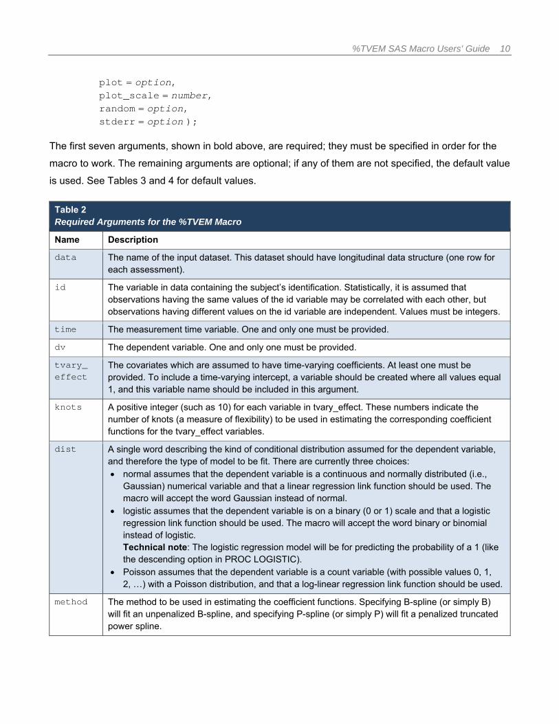
The first seven arguments, shown in bold above, are required; they must be specified in order for the

macro to work. The remaining arguments are optional; if any of them are not specified, the default value

is used. See Tables 3 and 4 for default values.

Table 2 Required Arguments for the %TVEM Macro

Name Description

data The name of the input dataset. This dataset should have longitudinal data structure (one row for each assessment).

id The variable in data containing the subject’s identification. Statistically, it is assumed that observations having the same values of the id variable may be correlated with each other, but observations having different values on the id variable are independent. Values must be integers.

time The measurement time variable. One and only one must be provided.

dv The dependent variable. One and only one must be provided.

tvary_ effect

The covariates which are assumed to have time-varying coefficients. At least one must be provided. To include a time-varying intercept, a variable should be created where all values equal 1, and this variable name should be included in this argument.

knots A positive integer (such as 10) for each variable in tvary_effect. These numbers indicate the number of knots (a measure of flexibility) to be used in estimating the corresponding coefficient functions for the tvary_effect variables.

dist A single word describing the kind of conditional distribution assumed for the dependent variable, and therefore the type of model to be fit. There are currently three choices: normal assumes that the dependent variable is a continuous and normally distributed (i.e.,

Gaussian) numerical variable and that a linear regression link function should be used. The macro will accept the word Gaussian instead of normal.

logistic assumes that the dependent variable is on a binary (0 or 1) scale and that a logistic regression link function should be used. The macro will accept the word binary or binomial instead of logistic. Technical note: The logistic regression model will be for predicting the probability of a 1 (like the descending option in PROC LOGISTIC).

Poisson assumes that the dependent variable is a count variable (with possible values 0, 1, 2, …) with a Poisson distribution, and that a log-linear regression link function should be used.

method The method to be used in estimating the coefficient functions. Specifying B-spline (or simply B) will fit an unpenalized B-spline, and specifying P-spline (or simply P) will fit a penalized truncated power spline.


Table 3 Important Optional Arguments for the %TVEM Macro

Name Description Default

invar_effect The covariates, if any, which are assumed to have a non-time-varying effect. Variables listed here must not be listed in tvary_effect.

If omitted, there will be no non-time-varying-effects variables in the model.

plot The technical mechanism used to plot the coefficient functions. Specify full to generate polished-looking plots; however, some users’ SAS or Java installations may not work with this option. Specify simple to generate a less polished-looking plot that is likely to work in more systems. Specify none to suppress plotting; this would mainly be used in loops or simulations in which the macro is being called many times.

full -Try simple if this does not work.

random The method to be used in estimating within-subject correlation. Specify none to estimate no within-subjects variability; this is not recommended unless there is only one observation per subject. Specify intercept to estimate a

random intercept for each subject. Specify slope to estimate both a random intercept and a random slope for each subject.2

slope -Try intercept if this does not work.

Last, there are arguments that most users will not have to change. Only users who are very familiar

with TVEM or who have specialized needs will wish to use them.

2 The random option is currently relevant only if the B-spline method is being used; it is ignored if the P-spline method is being used, because within-subject correlation is accounted for differently in that case.


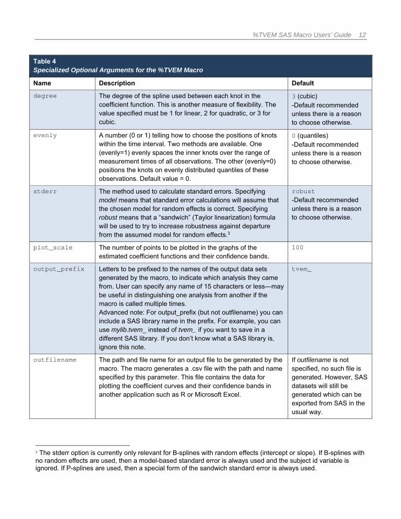
Table 4 Specialized Optional Arguments for the %TVEM Macro

Name Description Default

degree The degree of the spline used between each knot in the coefficient function. This is another measure of flexibility. The value specified must be 1 for linear, 2 for quadratic, or 3 for cubic.

3 (cubic) -Default recommended unless there is a reason to choose otherwise.

evenly A number (0 or 1) telling how to choose the positions of knots within the time interval. Two methods are available. One (evenly=1) evenly spaces the inner knots over the range of measurement times of all observations. The other (evenly=0) positions the knots on evenly distributed quantiles of these observations. Default value = 0.

0 (quantiles) -Default recommended unless there is a reason to choose otherwise.

stderr The method used to calculate standard errors. Specifying model means that standard error calculations will assume that the chosen model for random effects is correct. Specifying robust means that a “sandwich” (Taylor linearization) formula will be used to try to increase robustness against departure from the assumed model for random effects.3

robust -Default recommended unless there is a reason to choose otherwise.

plot_scale The number of points to be plotted in the graphs of the estimated coefficient functions and their confidence bands.

100

output_prefix Letters to be prefixed to the names of the output data sets generated by the macro, to indicate which analysis they came from. User can specify any name of 15 characters or less—may be useful in distinguishing one analysis from another if the macro is called multiple times. Advanced note: For output_prefix (but not outfilename) you can include a SAS library name in the prefix. For example, you can use mylib.tvem_ instead of tvem_ if you want to save in a different SAS library. If you don’t know what a SAS library is, ignore this note.

tvem_

outfilename The path and file name for an output file to be generated by the macro. The macro generates a .csv file with the path and name specified by this parameter. This file contains the data for plotting the coefficient curves and their confidence bands in another application such as R or Microsoft Excel.

If outfilename is not specified, no such file is generated. However, SAS datasets will still be generated which can be exported from SAS in the usual way.

3 The stderr option is currently only relevant for B-splines with random effects (intercept or slope). If B-splines with no random effects are used, then a model-based standard error is always used and the subject id variable is ignored. If P-splines are used, then a special form of the sandwich standard error is always used.


About spline basis: Should I use B‐spline or P‐spline?

Summary recommendation. Use P-spline for a quick understanding of your data. Then, select the

proper number of knots using B-spline to see the proper level of detail in the association you are

modeling.

Details. A spline is a shape composed of linear or quadratic segments. The so-called “knots” are the

places where these segments join together. Splines are useful because they allow great flexibility when

estimating the shape of a nonlinear function. There are various mathematical ways to represent a

spline. In particular, when writing code to run the %TVEM macro, you will need to select either a P-

spline or a B-spline. If you do not understand the difference, follow this procedure:

We recommend users start with a P-spline and a large number of knots (10 or more). The macro will

use the P-spline penalty to automatically select a good amount of smoothness (read more in Section

4.5) and will use sandwich standard errors that do not require further adjusting. P-spline, then, gives

you an immediate picture of the relationship you are modeling.

Once you have the big picture, you can optionally fine-tune the analysis using B-spline. When you use

B-spline, you must run the model multiple times, incrementally increasing or decreasing the number of

knots each time, in order to select the ideal model. This method is more sensitive than P-spline and can

reveal more detail. B-spline also allows users to specify random effects using the random argument.

For more details, see the examples in Sections 6.3 and 6.6.

Selecting the proper number of knots

When using P-spline, the correct number of knots will be selected by the macro if you select an

adequate number of knots; we recommend 10. The number selected must be entered for each variable

listed in the tvary_effect argument.

When using B-spline, select a low starting value and increment the number of knots. For example,

change the value in the knots argument from knots = 2 to knots = 3, to knots = 4, etc., running

your model each time. Then, select the correct number of knots by comparing the fit statistics in the

output. You can also choose the optional deg argument in this way, although it is also okay to leave

deg at its default value. However, it may be easier try to change only one aspect of the code (such as

the number of knots) at a time to avoid confusion when comparing many sets of output. Also, for

reasons described below, the random effects structure cannot be chosen using fit statistics in the same

way.


Specifically, when fitting a non-normal model with random effects, we use a pseudolikelihood method

within PROC GLIMMIX. That means that GLIMMIX estimates the coefficients by repeatedly

approximating the binary or Poisson model with better- and better-fitting weighted normal models,

which makes the computation much easier. However, this means that the log-likelihood, AIC, and BIC

fit statistics are based on a different distribution, known as the “pseudolikelihood” because it is the

approximating distribution, rather than an actual binary distribution. This means that the likelihood, AIC,

and BIC statistics cannot be compared between models with and without random effects in this macro.

However, they can be used to select the number of knots in the usual way within a choice of random

effects or no random effects.

Choosing how to model within‐subject correlation

When multiple observations are taken from each individual in a sample, it is well known that

observations within an individual are likely to be correlated with each other, and that some adjustment

should be made to account for the lack of independence. There are several ways to do this. Two of the

most commonly used are a (a) “robust” or “sandwich” standard errors and (b) random effects (also

known as mixed or multilevel modeling). The first method calculates the estimates as though the

observations were independent and then adjusts the standard errors to account for the fact that they

are not. The second method includes special terms in the model to account for the different

characteristics of each individual. For reasons described in the technical details section, we use the first

method with P-splines and the second method with B-splines. No action is required from the user for

the first method; the adjustment is done automatically. However, the user does have to make choices in

the second method.

Specifically, with B-splines you may use either (a) no random effect, (b) a random intercept only, or (c)

a random intercept and random slope. In general, random quadratic or higher-level effects are not

supported by the current version of the macro. Including no random effects treats all observations as

independent. Including only random intercepts treats all observations within the same person as equally

correlated. Including random intercept and random slope assumes that within the same person,

observations closer in time are more highly correlated than those further away. Including both a random

intercept and random slope is the richest and most realistic of these three choices. However, having

additional random effects can make a model too complicated to fit easily on a given data set. The

model might fail to converge if there is not sufficient information in the data set to estimate both the

regression model and also the random effects. For this reason, it might be wise to try the random slope


and random intercept first, and then try a simpler model, with random intercept only, if the richer model

fails.

For reasons described above, in the context of this macro, it isn't valid to use AIC or BIC to choose the

random effects structure. You could, however, get at least a rough idea of whether a particular kind of

random effect (slope or intercept) is accounting for a statistically significant amount of variability by

comparing the size of the estimated variance component to its standard error (both are shown in the

output). The ratio of the estimated variance component to its standard error is not exactly a valid test

statistic in the usual way (as though it were a z score), but it could be helpful as a heuristic. Another

approach is to include both a random slope and intercept if this model converges, but try a simpler

model if it does not.


Output The TVEM macro produces three different kinds of output, and optionally a fourth. Each is described

below.

Text output

Some summary output is provided on the screen (Results window) or listing (if in batch mode). If the B-

spline method is being used, this summary output includes the log-likelihood and information criteria

which can be useful for model selection. If the P-spline method is being used, these criteria are

currently not shown, because a penalty function is being applied to select the degree of model

complexity, and this indirectly creates certain complications for interpreting information criteria. If there

are any non-time-varying-covariates, then their estimates, standard errors, and p-values are shown.

Plots

For each time-varying coefficient, a plot is drawn to show how its relationship with the dependent

variable, as expressed by its estimated coefficient function , changes over time. Pointwise

confidence bands created to have 95% confidence using standard techniques are also shown. These

are pointwise confidence bands and do not imply joint confidence over all points together.

( )j ijt

Figure 1. Example Text Output

Intercept Only Model TVEM Macro Output Summary

=========================================================== Time-Varying Effects Modeling (TVEM) Macro Output =========================================================== Dataset: exampledata Time variable: Time Response variable: Urge Response distribution: Normal (Gaussian) Non-time-varying effects: Location1 Location2 Male Time-varying effects: Intercept Knots for splines: 10 Degree for splines: 3 Number of observations used: 5308 Internal computations in PROC GLIMMIX converged successfully. =========================================================== The estimated coefficient functions are stored in the dataset tvem_plot_data. ===========================================================


For logistic regression, in addition to the

coefficient function, the odds ratio function

(found by exponentiating ) is also

plotted separately. In a previous version

of the TVEM, this had to be specifically

requested using an option; it is now

provided automatically.

Plots are available in two formats, the

full version, which is generated by

default, and the simple version, which is

generated when you argument specify

plot = simple in your syntax. The

simple version is available for users whose machines fail to generate the full plots.

SAS datasets

Several SAS datasets are automatically produced by the macro. They have specific names describing

their contents, but you can optionally add a common prefix to all of their names as a way of marking

which analysis they came from, if you wish to run the TVEM macro more than once and compare the

results. The default prefix is just “Tvem_” if no other is specified.

Note: These datasets can be found in

the SAS Work directory. That is, you

can use them during the SAS session

but they disappear when you close

SAS. A LIBNAME and data step are

needed to save the files to permanent

SAS datasets on your hard drive or

network.

Not all of these datasets are produced

by all analyses (it depends on which

options are chosen), and not all of

these datasets will be meaningful for all

( )j ijt

Figure 2. Full Plot

Figure 3. Simple Plot


users. In fact, most users will not need the datasets, except perhaps for plot_data and/or plot_data_OR.

The other datasets are either duplicates of material shown in the screen output (e.g., fit statistics) or

else are very technical and of interest only for specialized situations (e.g., estimates and covariance

matrix of the coefficients for the individual basis functions, which would be interesting mainly to a

methodological researcher studying the performance of different spline methods). These files and their

contents are described in Table 4.


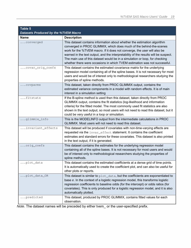
Table 5 Datasets Produced by the %TVEM Macro

Name Description

...converged This dataset contains information about whether the estimation algorithm converged in PROC GLIMMIX, which does much of the behind-the-scenes work for the %TVEM macro. If it does not converge, the user will also be warned in the text output, and the interpretability of the results will be suspect. The main use of this dataset would be in a simulation or loop, for checking whether there were occasions in which TVEM estimation was not successful.

...covar_orig_coefs This dataset contains the estimated covariance matrix for the underlying regression model containing all of the spline bases. It is not necessary for most users and would be of interest only to methodological researchers studying the properties of spline methods.

...covparms This dataset, taken directly from PROC GLIMMIX output, contains the estimated variance components in a model with random effects. It is of main interest in a simulation setting

...fitstats If the B-spline method is used then this dataset, taken directly from PROC GLIMMIX output, contains the fit statistics (log-likelihood and information criteria) for the fitted model. The most commonly used fit statistics are also shown in the text output, so most users will not need to read this dataset, but it could be very useful in a loop or simulation.

...glimmix_info This is the MODELINFO output from the intermediate calculations in PROC GLIMMIX. Most users will not need to read this dataset.

...invariant_effects This dataset will be produced if covariates with non-time-varying effects are requested via the invar_effect statement. It contains the coefficient estimates and standard errors for these covariates. This dataset is also printed in the text output, if it is generated.

...orig_coefs This dataset contains the estimates for the underlying regression model containing all of the spline bases. It is not necessary for most users and would be of interest only to methodological researchers studying the properties of spline methods.

...plot_data This dataset contains the estimated coefficients at a dense grid of time points. It is automatically used to create the coefficient plot, and can also be useful for other plots or reports.

...plot_data_OR This dataset is similar to plot_data, but the coefficients are exponentiated to base e. In the context of a logistic regression model, this transforms logistic regression coefficients to baseline odds (for the intercept) or odds ratios (for covariates). This is only produced for a logistic regression model, and it is also automatically plotted.

...predicted This dataset, produced by PROC GLIMMIX, contains fitted values for each observation.

Note. The dataset names will be preceded by either tvem_ or the user-specified prefix.


External file (optional)

If a valid Windows path and file name are provided for the outfilename argument in the macro, then the

contents of the plot_data dataset will be automatically exported to a comma-separated (.csv) text file,

which can be read in R or Microsoft Excel in order to create customized plots based on the estimated

coefficient functions. You can also export the dataset by using the SAS top menu, right-clicking the

dataset name, or calling PROC EXPORT.


Data Analysis Examples

Included with the macro is a simulated dataset based very loosely on intensive longitudinal studies of

smoking cessation such as the one described in Shiffman et al. (2002).

In the very simplified scenario used in the dataset, 200 individuals who want to stop smoking are

followed for 7 days after their quit attempt begins. At up to 30 random occasions during the week, they

are randomly prompted by an electronic device to describe their feelings. Their levels of negative affect

(distress, anxiety and sadness) and their levels of urge to smoke are recorded on a 0 to 10 scale. They

are asked to answer yes or no to a question that asks whether they currently think their quit attempt will

be successful. They also tell their location: whether they are at work, at home, or in a social or fun

setting.

Data preparation: Adding an intercept, recoding, and adding a title

Before running the TVEM analysis, we have to use the INCLUDE function to get SAS to read the macro

file.

%INCLUDE "C:\Users\MeMyself\Documents\Sims-Tvem\Tvem_v310.sas";

The data may need to be altered at this point using a data step. Below we create an intercept column

and dummy code a three-level variable to create two separate two-level variables. The data preparation

needed will be specific to each analysis.

/* Simulate data */ DATA exampledata;

SET here.exampledata; * Create an intercept column:;

Intercept = 1; * Dummy-code the three-level location variable:; Location1 = 0; IF Location=1 THEN Location1 = 1; Location2 = 0; IF Location=2 THEN Location2 = 1; RUN;

If you plan to run the macro several times (for example, if you select different numbers of knots), you

can add a title to each macro run in the output. This can be done by preceding your macro syntax with

a SAS command title like


Title "The first one";

The title will now appear as part of your macro output. To stop adding this title, just use the title command

again either to specify a new title, or to specify no title at all. In the latter case you simply type

Title;

Example with a normal distribution

Now we can use TVEM. We could start by studying how urge to smoke changes, on average, over time, adjusting for subject’s sex (coded as a dummy variable with 1=male, 0=female) and location (coded as above). We could start with an intercept-only TVEM, which reduces to simply a smoothed nonparametric regression of the dependent variable on time.

%TVEM(dist=normal, data = exampledata, id = SubjectID, time = Time, dv = Urge, tvary_effect = Intercept, method = P-spline, knots = 10, invar_effect = Location1 Location2 Male);

The output for fixed effects covariates

suggests that participants had lower urge

to smoke while at work. The effect of male

gender seems significant using the model-

based standard errors under the

assumption of independent observations,

but not significant using a robust standard

error. However, the effect of location 1

remains very strongly significant.

The plot suggests that average urge to

smoke increased and then decreased as

the week went on. Note that this is the

“full” version of the plot because the plot

argument was not specified.

Figure 4. Example 6.2: Plot


Table 6 Example 6.2: Fixed Effects Covariates Output

Obs Effect Estimate StdErr RobustStdErr ModelBasedZ RobustZ ModelBasedP RobustP

1 Location1 -0.07503 0.03516 0.03165 -2.13415 -2.37090 0.032831 0.01774

2 Location2 0.06805 0.03747 0.03680 1.81587 1.84935 0.069390 0.06441

3 Male 0.09339 0.02988 0.11023 3.12498 0.84717 0.001778 0.39690

Example with normal distribution using B‐spline

We can include random effects as follows.

%TVEM( dist=normal, data = exampledata, id = SubjectID, time = Time, dv = Urge, tvary_effect = Intercept, method = B-spline, knots = 2, random = slope, invar_effect = Location1 Location2 Male);

In practice we should try different values of knots to try to get a good AIC or BIC. To do this, we would

use the same code, but use knots = 3, then knots = 4, etc. We would select the correct number of

knots by the fit statistics in the output. (NOTE: Here we should keep the other aspects of our code the

same while incrementing the number of knots, so that the comparison of fit statistics will apply directly

to the question of the selection of knots.)

The resulting plot is rather similar (not shown), but we now see some new output (Tables 7 and 8).

It appears that there is both a random intercept and a random slope over time, although the random

intercept seems to be more important.


Example with a time‐varying covariate

Now let us include a covariate, namely NegAffect, which may have a time-varying effect. We might

run the following code:

%TVEM(dist=normal, data = exampledata, id = SubjectID, time = Time, dv = Urge, tvary_effect = Intercept NegAffect, method = P-spline, knots = 10 10, invar_effect = Location1 Location2 Male);

which will produce the plots in Figure 5.

It appears that the effect of negative affect on urge to smoke in this dataset is always significant and

positive, and tends to increase over time.

Table 7 Example 6.3: Fixed Effects Covariates Output

Obs Effect Estimate StdErr DF tValue

1 Location1 -0.1098 0.02529 6644 -4.34

2 Location2 0.04233 0.03020 6644 1.40

3 Male 0.1091 0.1038 6644 1.05

Table 8 Example 6.3: Covariance Parameters

Obs CovParm Subject Estimate StdErr

1 Intercept SubjectID 0.4330 0.05062

2 Time SubjectID 0.007879 0.001328

3 Residual 0.9196 0.01592


Example with a logistic distribution

In the same dataset, we also have simulated binary data: the participant’s prediction as to whether he

or she will be able to quit in the long-term. Let’s try fitting a TVEM to predict the success expectancy

from urge.

%TVEM(dist = logistic, data = exampledata, id = SubjectID, time = Time, dv = ExpectedSuccess, tvary_effect = Intercept Urge, method = P-spline, knots = 10 10 , invar_effect = Location1 Location2 Male);

In Figure 6, It appears from the plot on the left that confidence declines over time after adjusting for

urge. It appears from the plot on the right that urge has a generally negative relationship with

confidence, more so as time goes on.

Figure 5. Example 6.4: Plots


Exponentiated versions of these curves are also generated, showing the time-specific odds of

expecting success, and the odds ratio of expecting success between people differing by one unit of

urge (See Figure 7).

We do not see any effect of location on confidence in one’s quitting ability, unlike when we were

predicting urge (Table 9).

Figure 7. Example 6.5: Quadratic Plots

Figure 6. Example 6.5: Linear Plots


Example with logistic outcome using B‐spline

We can also include random effects in this analysis. We try the following code:

%TVEM(dist=logistic, data = exampledata,

id = SubjectID, time = Time, dv= ExpectedSuccess, tvary_effect = Intercept Urge, method = B-spline,

knots = 2 2 , random = slope,

invar_effect= Location1 Location2 Male);

In the output (Table 10), we see a noticeable random intercept but not much of a random slope.

Table 10 Example 6.6: Covariance Parameters

Obs CovParm Subject Estimate StdErr

1 Intercept SubjectID 0.2150 0.04569

2 Time SubjectID 0.003040 0.003052

Table 9 Example 6.5: Fixed Effects Covariates

Obs Effect Estimate StdErr RobustStdErr ModelBasedZ RobustZ ModelBasedP RobustP

1 Location1 0.001619 0.07020 0.068221 0.02306 0.02373 0.98160 0.98107

2 Location2 0.01957 0.07495 0.073885 0.26105 0.26480 0.79406 0.79116

3 Male 0.1265 0.06000 0.089297 2.10898 1.41694 0.03495 0.15650


Technical Details on Spline Bases

Without loss of generality, we consider the following generalized time-varying coefficient model

(Equation 4), which we show here again for convenience:

, ⋯ .

B‐spline basis

The process of estimating the unknown coefficient function ∙ involves approximating this function

with certain combinations of B-spline basis functions that are determined by knots and degree. Given

m+1 knots, say, ⋯ , the m-d basis B-splines of degree d can be defined using the Cox-

de Boor recursion formula (de Boor, 1972) with

and

.

In addition, knots ⋯ are called internal knots (or inner knots). In the %TVEM

macro, the knots , ⋯, and , ⋯, are determined by the minimal ( ) and the maximal

( ) observation time in the input data set as follows:

1 , 0, 1, 2,⋯ ,, ,

where is a small positive number that is set at in this macro. In addition, we employ cubic splines

( 3) in this macro, as many applications do.

Given the number of inner knots, the inner knots are equally distributed over the range of the study

period or uniformly distributed on quantiles of measurement times (depending on the designation in the

evenly parameter). For example, suppose that the study period is from year 0 to year 1. If we use four

knots and distribute them equally over the study period, the inner knots will be at year 0.2, 0.4, 0.6, and

1

,01

1, t{ }

0, <t or

j j

jj t

bt t

tt

t t

1, , 1 1, 1

1 1

( ) ( ) ( ), for 0,1, , 1j j dj d j d j d

j d j j d j

t t t tb b

t tb t t t j K

t td

1210


0.8. Or, if we distribute the 4 inner knots uniformly on the quantiles of measurement times, they will be

at the 20%, 40%, 60% and 80% quantiles of the pooled measurement times.

Hence, when we input the number of inner knots = k (using the knots parameter), and we define the

method to posit these inner knots (using the evenly parameter), the %TVEM macro will calculate the

inner knots, and then all the 2 1 knots, and then 1 B-spline basis functions by using

the Cox-de Boor recursion formula. For example, if = 4, then there are 8(=4+3+1) cubic B-spline

basis functions.

To estimate the coefficients in Equation 4, we approximate ∙ by k +3+1 cubic B-spline basis

functions:

(5)

where , ∙ , j= 0, 1, ⋯, k+3, are cubic B-spline basis as defined by the Cox-de Boor recursion formula,

and , j= 0, 1, ⋯, k+3, are unknown parameters. In this way, we transfer the problem of estimating the

function ∙ into a problem of estimating , 0, 1,⋯ , 3. Combining Equations 4 and 5, we get

the following regression model:

, , .

The estimate of , 0, 1,⋯ , 3, can be obtained using available software, such as the PROC

GENMOD or the GLM package in R. The number of inner knots determines the number of basis

functions used to approximate ∙ . Intuitively, the larger the number of inner knots, the better the

approximation. However, using too many basis functions could cause over-fitting, which can cause near

interpolation of the data and undesirable “wiggly” curves. So, we need to select the ideal number of

inner knots to ensure good approximation and avoid over-fitting. This can be done by using different

numbers of inner knots and running the model repeatedly. Then, we select the optimal number based

on the model fit statistics (AIC and/or BIC) provided in the output.

3

0 ,30

( ) ( )K

j jk

tt a b


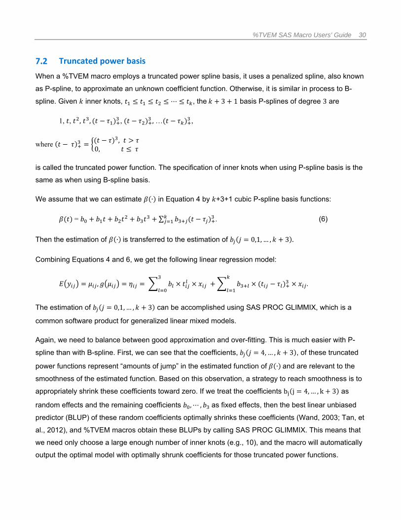
Truncated power basis

When a %TVEM macro employs a truncated power spline basis, it uses a penalized spline, also known

as P-spline, to approximate an unknown coefficient function. Otherwise, it is similar in process to B-

spline. Given inner knots, ⋯ , the 3 1 basis P-splines of degree 3 are

1, , , , , , … ,

where ,0,

is called the truncated power function. The specification of inner knots when using P-spline basis is the

same as when using B-spline basis.

We assume that we can estimate ∙ in Equation 4 by +3+1 cubic P-spline basis functions:

= ∑ . (6)

Then the estimation of ∙ is transferred to the estimation of 0,1, … , 3 .

Combining Equations 4 and 6, we get the following linear regression model:

, .

The estimation of 0,1, … , 3 can be accomplished using SAS PROC GLIMMIX, which is a

common software product for generalized linear mixed models.

Again, we need to balance between good approximation and over-fitting. This is much easier with P-

spline than with B-spline. First, we can see that the coefficients, 4,… , 3 , of these truncated

power functions represent “amounts of jump” in the estimated function of ∙ and are relevant to the

smoothness of the estimated function. Based on this observation, a strategy to reach smoothness is to

appropriately shrink these coefficients toward zero. If we treat the coefficients b j 4, … , k 3 as

random effects and the remaining coefficients , ⋯ , as fixed effects, then the best linear unbiased

predictor (BLUP) of these random coefficients optimally shrinks these coefficients (Wand, 2003; Tan, et

al., 2012), and %TVEM macros obtain these BLUPs by calling SAS PROC GLIMMIX. This means that

we need only choose a large enough number of inner knots (e.g., 10), and the macro will automatically

output the optimal model with optimally shrunk coefficients for those truncated power functions.


Technical differences between using B‐spline and P‐spline

In summary, there are two main differences between using B-spline and using P-spline: (a) to

approximate unknown coefficient functions, B-spline uses a B-spline basis, and P-spline uses a

truncated power basis; and (b) to automatically counter over-fitting due to the large number of inner

knots, P-spline uses a penalty (through the use of a mixed-effect model), but in B-spline this is done

manually by comparing model fit statistics of different models using different numbers of knots. Note

that the syntax B-spline refers to using a B-spline basis with a spline that is not penalized and the

syntax P-spline refers to using penalized spline with a truncated power basis.

In general, P-spline will produce smoother estimates of coefficient functions than B-spline. Using P-

spline frees the user from needing to try multiple models with different numbers of knots. However,

truncated power basis functions can be highly correlated (i.e., multicollinear), which may cause

numerical instability in computation. B-spline basis functions, on the contrary, are locally independent

and hence are numerically stable in computation.

It would be reasonable to ask why random effects are not available for P-splines. The reason is that the

usual method for determining the optimal penalty strength in P-splines is computationally nontrivial. It is

not very difficult in itself, but when combined with also estimating random effects it could cause

convergence difficulties in estimation.Therefore, we chose to limit P-splines to the simpler approach of

robust standard errors without random effects.

Technical details about random effects

When random effects are used, Equation 4 for the expected value of observation j on subject i is

replaced by

, ⋯ , (7)

where ai and bi are the random intercept and slope for the ith person. The ai and bi are assumed

independent normal with mean zero and with variances and . If only a random intercept and not a

random slope are used, then the term is omitted in Equation 7 (essentially assuming 0 so

that everyone has a bi of zero).

Equation 7 has an unexpected but important consequence regarding the measurement of time. Usually,

for TVEM, the scale on which time is measured does not matter very much; it simply changes the

labeling of the x-axis of the coefficient plot. That is, for Equation 4 it doesn’t matter much whether is


counted from 0 to 1, -1 to 1, 1 to 10, or 1950 to 2050. However, for Equation 7 the scaling of time

matters much more, because the slope bi is a contrast of the current time with time zero. In other

words, the variance of the random effects at time t, from Equation 7, is

Var( , (8)

and time zero now has a special meaning as the point at which this function reaches its minimum. To

see why this matters, consider a practical example.

Suppose that a researcher is studying the change in alcohol use in a sample of young people, starting

in the calendar year 2005 (when they were all 13 years old) and ending in the calendar year 2015

(when they were all 23 years old). Should the first year of the study be coded as 0 (because it is the

beginning of the study), as 13 (because the participants were thirteen years old), or 2005 (because that

was the calendar year)? Ordinarily, the %TVEM macro can handle any of these three possibilities, and

the researcher can use whatever metric is convenient. However, if a random slope is being used then

the meaning of the coefficients in the model changes drastically. If the subject’s age is used, then the

random effects are estimated by extrapolating back to the subject’s birth, years before the study began.

This is unfortunate, but maybe not disastrous. However, if the calendar year is used, then the random

effects are estimated by extrapolating back to the calendar year zero, many centuries before the

participants were born. In this extreme case, the estimation algorithm probably would not converge, and

even if it did converge the estimates would not have any interpretable meaning. Thus, in order to use a

random slope the investigator will have to define the time variable as time from some event which is

meaningful to the study (such as the start of the study, onset of adolescence, beginning of treatment, or

whatever is deemed appropriate). This caveat is not specific to random effects TVEM, but arises in

multilevel modeling in general, whenever a random slope is being used.

Even after deciding about the beginning point of measurement, the investigator might still have a

question about the units or scale of measurement. Should the time variable be defined as weeks,

months, years, or decades since the start of the study? Any of these could be meaningful, and none of

them are wrong. However, they will lead to different estimates of the variance . This is because, if t is

12 times larger (a number of months instead of years), then must be 144 times smaller in order to

provide the same in Equation 8. This is not inherently a problem. However, it does mean that a

seemingly very small number for the random slope variance (maybe .001) might still represent an

important variance component. That is because the absolute size of the number could be smaller or

larger if the units of time were different. Fortunately, in the macro output, the estimated variance


components are provided side by side with standard errors for these estimates. The standard error is

scaled appropriately for the variance component, and when thinking about the significance of the

variance component it would be more reasonable in this case to compare it to its standard error than to

look at its absolute size.


References

Buu A., Johnson, J. J., Li, R., & Tan, X. (2010). New variable selection methods for zero-inflated count

data with applications to the substance abuse field. Statistics in Medicine, 30(18), 2326-2340.

de Boor, C. (1972). On calculating with B-splines. Journal of Approximation Theory, 6, 50–62.

Erdman, D., Jackson, L., & Sinko A. (2008). Zero-inflated Poisson and zero-inflated negative Binomial

models using the COUNTREG procedure. SAS Global Forum 2008, paper 322.

Hastie, T. J., & Tibshirani, R. J. (1993). Varying-coefficient models (with discussion). Journal of the

Royal Statistical Society B, 55, 757-796.

McCullagh, P., & Nelder, J. (1989). Generalized linear models (2nd ed.). Boca Raton, FL: Chapman and

Hall/CRC.

Shiffman, S., Gwaltney, C. J., Balabanis, M. H., Liu, K. S., Paty, J. A., Kassel, J. D., Hickcox, M., &

Gnys, M. (2002). Immediate antecedents of cigarette smoking: an analysis from ecological

momentary assessment. Journal of Abnormal Psychology, 111(4), 531-545.

Shiyko, M. P., Lanza, S. T., Tan, X., Li, R., & Shiffman, S. (2012). Using the time-varying effect model

(TVEM) to examine dynamic associations between negative affect and self-confidence on

smoking urges: differences between successful quitters and relapsers. Prevention Science.

Advance online publication. doi: 10.1007/s11121-011-0264-z

Tan, X., Shiyko, M. P., Li, R., Li, Y., & Dierker, L. (2012). A time-varying effect model for intensive

longitudinal data. Psychological Methods, 17, 61 77.

Tiffany, S. T., Agnew, C. R., Maylath, N. K., Dierker, L., Flaherty, B., Richardson, E., ..., Tobacco

Etiology Research Network (TERN). (2007). Smoking and college freshmen: University project of

the Tobacco Etiology Research Network (UpTERN). Nicotine & Tobacco Research, 9(S4), S611-

S625.

Wand, M. P. (2003). Smoothing and mixed models. Computational Statistics, 18, 223-249.