two essays on the role of nonbank financial …
TRANSCRIPT

TWO ESSAYS ON THE ROLE OF NONBANK FINANCIAL
INSTITUTIONS AND FIRMS IN THE MONETARY
TRANSMISSION MECHANISMS
by
Sung-Eun Yu
A dissertation submitted to the faculty of The University of Utah
in partial fulfillment of the requirements for the degree of
Doctor of Philosophy
Department of Economics
The University of Utah
August 2015

Copyright © Sung-Eun Yu 2015
All Rights Reserved

The University of Utah Graduate School
STATEMENT OF DISSERTATION APPROVAL
The following faculty members served as the supervisory committee chair and
members for the dissertation of____________________________________________.
Dates at right indicate the members’ approval of the dissertation.
_________________________________________, Chair ________________ Date Approved ________________________________________, Member ________________ Date Approved ________________________________________, Member ________________ Date Approved ________________________________________, Member ________________ Date Approved ________________________________________, Member ________________ Date Approved The dissertation has also been approved by__________________________________
Chair of the Department/School/College of____________________________________
and by Charles A. Wight, Dean of The Graduate School.
Sung-Eun Yu
Lance Girton
Stephen Reynolds
James Gander
David Kiefer
Rungrudee Suetorsak
Thomas Maloney
Economics
1/14/2015
6/9/2015
2/23/2015
1/22/2015
3/5/2015

ABSTRACT
In my first essay, I theoretically and quantitatively examine the role of nonbank
financial institutions in the monetary transmission mechanisms. First, in accordance
with Bernanke’s proposal (2007), I theoretically explain the effect of restrictive
monetary policy on the behavior of both banks and nonbank financial intermediaries
through their balance sheet conditions, which is a medium for the two kinds of lenders
to shrink their loan supply. Second, if this theoretical explanation is correct, empirically
we should expect the net worth and the intermediated loans of both kinds of lending
institutions to fall in response to a tight monetary shock. Employing the traditional OLS
and the VAR methodology, I find that nonbank financial institutions respond by
shrinking their net worth, and they subsequently reduce their loans in the same ways
banks do. This evidence suggests that nonbank financial institutions may play an
important role in amplifying the effect of monetary policy on output, providing some
explanation of the existing puzzles.
In my second essay, I provide more evidence on the behavior of small and large
firms, employing the Flow of Funds data, the QFR data and other sources. The
empirical test to examine behavior of small and large firms is conducted in two ways:
(1) by different episodes, tight monetary policy episodes and business cycles episodes
and (2) by different time periods, Pre-1990 periods and Post-1990 periods.

iv
First, I find that a monetary shock and an NBER recession shock differently affect
firms’ short-term financing behavior. During recent periods, after a contractionary
monetary shock, large firms increase their short-term debt more than small firms,
whereas after an NBER recession shock, large firms decrease most balance sheet
variables (including short-term debt) more than small firms. These findings suggest that
small firms are more credit-constrained after a monetary policy shock, whereas large
firms are more credit-constrained after an NBER recession shock. Second, I find that,
after a contractionary monetary shock, during earlier periods, large firms decrease their
short-term debt less than small firms, whereas during recent periods, large firms
increase more than small firms. Although these findings appear to be contradictory,
they are consistent in that small firms have continued to be more credit-constrained than
large firms after contractionary monetary policy―at the time when demand for loans
increases.

For my beloved parents and sisters

TABLE OF CONTENTS
ABSTRACT……………………………………………………………………….……iii
LIST OF FIGURES……………………………………………………………….……ix
LIST OF TABLES………………………………………………………………………x
Chapters
1. INTRODUCTION …………………………………………………………………1 1.1 References…………………………………………………………………..8
2. THE ROLE OF NONBANK FINANCIAL INSTITUTIONS IN THE MONETARY
TRANSMISSION MECHANISM: THEORY AND EVIDENCE ………………10 2.1 Introduction ………………………………………………………………10 2.2 An Overview of Nonbank Financial Institutions…………………………15
2.2.1 Changes in the Structure of the U.S. Financial System …………...16 2.2.2 The Growth of NBFIs ……………………………………………..23 2.2.3 Market Share of Credit ………………………………………….....26
2.3 A Theoretical Explanation ……………………………………….……….30 2.3.1 The External Finance Premium of Financial Intermediaries…….....30 2.3.1.1 The Impact of Monetary Policy on All Financial Intermediaries …………..…………………………….…….31 2.3.1.2 Specialness of Intermediated Loans in General………….…37 2.3.1.3 Expansion of the Bank Lending Channel …………………..40
2.4 Data Description and Methodology ………………………………………41 2.4.1 Data Description………………………………………….………...41 2.4.2 Methodology…………………………………………………….....42 2.4.2.1 A KSW-Style Approach…………………………………….43 2.4.2.2 A VAR Approach…………………………………………...47
2.5 Empirical Results………………………………………………………….50 2.5.1 The Impact of Monetary Policy on the Net Worth of Financial Intermediaries………………………………………………….…..51 2.5.2 The Impact of Monetary Policy on the Loans of Financial Intermediaries……………………………………………………...56

vii
2.6 Some Supplementary Tests for Loans for NBFIs………………………….63 2.6.1 A New Measure of Monetary Policy Shocks……………………….64 2.6.1.1 A Problem with the Conventional Measure ………………...64 2.6.1.2 The Derivation of a New Measure of Monetary Shocks…….65 2.6.1.3 Empirical Results …………………………………………...67 2.6.2 The Bank Lending Standards ………………………………………82
2.7 Conclusion ………………………………………………………………...89 2.8 Appendices ………………………………………………………………..92 2.8.1 A. Determination in the Number of Lags (VAR) …………………..92 2.8.2 B. Determination in the Number of Lags for Net Worth (OLS)……93 2.8.3 C. Responses of Net Worth (8 Lags)………………………………..93 2.8.4 D. Determination in the Number of Lags for Loans (OLS)………...94 2.8.5 E. Responses of Loans (2 Lags and 6 Lags)………………………...95 2.9 References ……………………………………………………………..….97
3. THE BEHAVIOR OF SMALL AND LARGE FIRMS DURING BUSINESS
CYCLE EPISODES AND DURING MONETARY POLICY EPISODES: A COMPARISON OF EARLIER AND RECENT PERIODS……………………..101
3.1 Introduction…………………………………………………….……........101 3.2 Data Description and Some Key Dates of Analysis……………………....108
3.2.1 Data Description……………………………………………….…..108 3.2.1.1 The Flow of Funds Data…………………………………....108 3.2.1.2 The Quarterly Finance Report Data………………………...109 3.2.1.3 The Senior Loan Officer Opinion Survey ……………….....110 3.2.1.4 The Business Employment Dynamics Data………………...111 3.2.2. Some Key Dates of Analysis…………………………………..….112 3.2.2.1 Dates of Business Cycle Peaks……………………………..113 3.2.2.2 Dates of Monetary Policy Shocks…………………………..114
3.3 Applying the Method of Previous Researchers to the Recent Data of the QFR……………………………………………….…………………..116 3.4 Empirical Results……………………………………………….………...122
3.4.1 The Responses of Small Versus Large Firms to the NBER Recessions………………………………………………………….122 3.4.1.1 The Flow of Funds Data and the QFR Data………………..123 3.4.1.2 The Senior Loan Officer Opinion Survey Data…………….131 3.4.1.3 The Business Employment Dynamics Data………………...135 3.4.2 The Responses of Small Versus Large Firms to Monetary Policy……………………………………………………………....147 3.4.2.1 The Flow of Funds Data and the QFR Data………………..147 3.4.3 Is a Monetary Policy Shock Different from an NBER Recession Shock? …………………………….…………….……..155 3.4.3.1 Lines of Credit……………………………………………...160 3.4.3.2 A Monetary Shock and the Availability of Credit Lines………………………………………………..162
viii
3.4.3.3 An NBER Recession Shock and the Availability of Credit Lines……………………………………………….165
3.4.3.4. Summary…………………………………………………..168 3.5 Why Do Large Firms Show Much More Sensitive Behavior of Short- term Debt in Response to an Adverse Shock?……………………………169 3.5.1 Financial Conditions of Borrowers………………………………...170 3.5.2 Benefits of Lending Relationships………………………………....175 3.5.3 Summary…………………………………………………………...182
3.6 Conclusion……………………………………………….………………..183 3.7 Appendices……………………………………………….…………….....187 3.7.1 A. Creating Time Series for the Small and Large Group…………..187 3.7.2 B. Cumulative Growth Rates of Sales after HP Filtering (15th Percentile Capital-based Division and Nominal Cut-off Division)…189 3.7.3 C. Average Changes in Inventories, Total Short-term Debt, Components of Aggregate Debt and Trade Debt Around Romer Dates………………………………………….……………………..190 3.7.4 D. The Behavior of Net Worth Between Small and Large Firms Measured by Using the QFR Data…………………………………….191
3.8 References……………………………………………….………………..192 4. CONCLUSION………………………………………………………………….....196 4.1 References……………………………………………….………………..201

LIST OF TABLES
2.1 Outstanding Assets Held by Financial Sector……………………………………24 2.2 Holding of Corporate Equity……………………………………………………..25 2.3 Responses of Net Worth………………………………….………………………52 2.4 Bivariate Model………………………………….……………………………….57 2.5 Multivariate Model……………………………………………………………….57 2.6 The Impact of New Monetary Policy Shocks on Total Loans …………………..72 2.7 The Impact of New Monetary Policy Shocks on Components of Loans (Banks) …………………………………………………………………………..73 2.8 The Impact of New Monetary Policy Shocks on Components of Loans (NBFIs) …………………………………………………………………………..74 2.9 The Impact of Conventional Funds Rate Shocks on Total Loans………………...79 2.10 The Impact of Conventional Funds Rate Shocks on Components of Loans (Banks) …………………………………………………………………………...80 2.11 The Impact of Conventional Funds Rate Shocks on Components of Loans (NBFIs) …………………………………………………………………………...81 3.1 Average Quarterly Level, Share, and Growth Rate of Gross Job Gains and Gross Job Losses by Firm Size (Seasonally Adjusted, 1992 Q3 to 2011 Q4)……………….138

LIST OF FIGURES
2.1 Distribution of Total Credit by Credit Type……………………………………..27 2.2 Total Credit………………………………………………………………………28 2.3 Commercial and Industrial Loans………………………………………………..28 2.4 Mortgages………………………………………………………………………..28 2.5 Consumer Loans…………………………………………………………………29 2.6 Responses of Net Worth…………………………………………………………55 2.7 Responses of Total Loans, C&I Loans, Mortgages, and Consumer Loans……...60 2.8 Responses of Total Loans, C&I Loans, Mortgages, and Consumer Credit to a One S.D. a New Measure Innovation…………………………………………....68 2.9 The Responses of Total Loans and Components of Loans to a Federal Funds Rate Shock and a New Measure Shock…………………………………………..76 2.10 Changes in C&I Loan Standards and Federal Funds Rate……………………….84 2.11 Responses of C&I Loans, GDP, Federal Funds Rate, Standards to One S.D. Standard Shock …………………………………………………………………..86 3.1 Log Deviation of U.S. GDP from HP Trend……………………………………113 3.2 Effective Federal Funds Rate…………………………………………………...115 3.3 Growth Rates of Sales…………………………………………………………..117 3.4 Cumulative Growth Rates of Sales……………………………………………...118 3.5 Cumulative Growth Rates of Sales After HP Filtering…………………………119 3.6 Sales of Small and Large Firms After an NBER Recession Shock…………….120

xi
3.7 Sales of Small and Large Firms After a Monetary Policy Shock……………….121 3.8 Average Sales of Small and Large Firms After Either an NBER Recession Shock or a Monetary Policy Shock………………………………….121 3.9 Average Changes in Sales and Some Balance Sheet Variables After an NBER Recession Shock ………………………………………………………………..124 3.10 Net Percentage of Domestic Respondents Tightening Standards for C&I Loans…………………………………………………………………………...132 3.11 Net Percentage of Domestic Respondents Increasing Spreads of Loan Rates over Banks’ Cost of Funds……………………………………………………...133 3.12 Net Percentage of Domestic Respondents Reporting Stronger Demand for C&I Loans………………………………………………………………………135 3.13 Gross Job Gain Rates and Gross Job Loss Rates……………………………….142 3.14 Net Job Creation and Net Job Creation Rates Between Small and Larger Firms, 1992 Q3 to 2011 Q4 …………………………………………………….143 3.15 Cumulative Employment Changes Since the Start of the 2001 and 2007-2009 Recessions ………………………………………………………….146 3.16 Average Changes in Sales and Some Balance Sheet Variables After a Monetary Policy Shock …………………………………………………………………....148 3.17 Average Changes in Total Short-term Debt and Short-term Bank Debt Around Beginning Dates of NBER Recessions ………………………………..156 3.18 Average Changes in Total Short-term Debt and Short-term Bank Debt Around Monetary Policy Shock ………………………………………………..157 3.19 Timing of a Monetary Policy Shock and an NBER Recession Shock …………163

CHAPTER 1
INTRODUCTION
Most economists would agree that monetary policy influences the real economy in
the short run. Yet, they would disagree on precisely how monetary policy influences the
real economy (see Bernanke & Blinder 1992; Christiano, Eichenbaum, & Evans 1996a,
1996b; Romer & Romer, 1989, for empirical evidence). Such different ways of how
monetary policy influences aggregate demand and output is referred to as monetary
transmission mechanisms. According to the conventional interest rate channel, the
actions of monetary authority influence consumption and investment spending through
changes in interest rates, therefore ultimately affecting the real economic activity. In
this interest rate channel, the effectiveness of monetary policy depends on interest-rate-
sensitive components of aggregate expenditure. However, empirical studies have faced
enormous difficulty in identifying the quantitatively strong effect of interest rates on
real variables, such as aggregate output and employment, in terms of purportedly
interest-rate-sensitive components of aggregate expenditure 1 (see Friedman, 1990;
Shapiro, Blanchard, & Lovell, 1986, for such difficulty in empirical studies).
The shortcomings of the conventional approach led a number of economists to
search for other complementary explanations, one of which is known as the credit
1 In other words, the estimated macroeconomic responses to policy induced interest rate changes are
substantially larger than those inferred by conventional estimates of the interest rate sensitivity of consumption and investment.

2
channel of monetary policy. It puts emphasis on the role of credit market imperfections.
In a situation where borrowers have more information about the quality of their projects
than do lenders, such asymmetric information can trigger a premium in the cost of all
forms of external finance over the cost of internal funds. This premium, known as an
external finance premium, compensates lenders for the costs of mitigating the problems
of moral hazard and adverse selection―e.g., the costs incurred in monitoring borrowers
and a lemon premium that results from asymmetric information problems. According to
the credit channel thesis, the impact of monetary policy on interest rates is magnified by
endogenous changes in the external finance premium. The external finance premium to
borrowers depends inversely on their financial conditions, measured in terms of
indicators such as net worth and liquidity. For example, a borrower who has a stronger
financial condition faces a lower external finance premium because the stronger
financial condition mitigates the borrower’s potential conflict of interest with a lender.
As a result, endogenous changes in borrowers’ financial conditions may increase the
persistence and amplitude of business cycles and make stronger the influence of
monetary policy. The credit channel therefore suggests that monetary policy can
influence the cost and availability of credit by more than implied by the conventional
movement in the interest rate channel alone.2
How do monetary policy actions affect the external finance premium in the credit
channel? Bernanke and Gertler (1995) explain two possible effects: the balance sheet
channel and the bank lending channel. First, according to the balance sheet channel,
monetary policy can influence the external finance premium of borrowers (especially
2 The credit channel of monetary policy is a magnification effect that works in tandem with the
interest rate channel―rather than a distinctive and independent alternative to the interest rate channel.

3
small firms) by changing their balance sheet conditions (Bernanke & Gertler 1995;
Gertler & Gilchrist 1991, 1993, 1994). For example, contractionary monetary policy
that increases interest rates deteriorates borrowers’ balance sheet conditions because an
increase in interest rates raises their debt services and drops the value of their
collateralizable assets. The weakening of borrowers’ financial conditions increases the
external finance premium, thereby reducing borrowers’ ability to access credit. Second,
according to the bank lending channel, monetary policy can influence the external
finance premium of borrowers (especially small firms) by shifting the supply of bank
loans away from small firms. For example, contractionary monetary policy that drains
reserve-backed deposits makes some banks unable to raise nondeposit source of funds
to continue their lending. If small firms are shut off from bank loans and are forced to
find a new lender, they must incur some costs (i.e., an increase in the external finance
premium) in establishing new credit relationships (Bernanke & Gertler, 1995). 3
Through either channel, contractionary monetary policy increases the external finance
premium of small firms who are subject to capital market imperfections. The effect of
the monetary policy action is amplified by endogenous changes in the external finance
premium.
3 The example shown here illustrates one way of operating the bank lending channel; tight monetary
policy influences the supply of bank loans by changing the external finance premium of nonfinancial firms. However, tight monetary policy can also influence the supply of bank loans by weakening the balance sheet conditions of financial firms―and thus by changing the external finance premium of financial firms. Such a way of operating the bank lending channel is shared by many other papers. Because banks must borrow uninsured funds in order to lend, they must pay the external finance premium just as ordinary firms do.
As banks’ balance sheet conditions become weak after contractionary monetary policy, banks must pay the higher external finance premium to continue lending, thus being forced to reduce their loan supply. In this case, the bank lending channel is the balance sheet channel as applied to the operations of banks. The bank lending channel essentially operates through banks’ balance sheet quality that results from either changes in bank reserves or changes in bank equity after monetary tightening (See Bernanke & Blinder 1988; Kashyap & Stein, 1995, 2000; Stein, 1998, for bank reserves and see Kishan & Opiela, 2000, 2006; Meh & Moran, 2004; Van den Heuvel, 2002, 2007, for bank equity)

4
My research is motivated by the unsatisfactory explanation of the conventional view
of monetary transmission mechanisms. In my dissertation, I therefore examine the
behaviors of lenders and the behaviors of borrowers more closely to find possible
explanations for the empirical difficulty we have faced. On the lenders’ side, I consider
the behavior of nonbank financial institutions―which previous studies fail to take into
account in the mechanism of monetary policy―as one possible contributing factor to
the sharp decline in output following tight monetary policy. Nonbank financial
institutions (NBFIs hereafter), which also provide credit to borrowers in credit markets,
may cut back on their credit to borrowers in a similar manner to banks if tight monetary
policy affects the behavior of both kinds of lending institutions in a similar way.
Chapter 2, entitled “The Role of Nonbank Financial Institutions in the Monetary
Transmission Mechanism: Theory and Evidence,” theoretically and quantitatively
examines the role of NBFIs in the transmission of monetary policy. First, as suggested
by Bernanke (2007), I theoretically explain how contractionary monetary policy affects
the quantity of loans of banks and NBFIs through changes in their balance sheet
conditions, particularly net worth. Second, I empirically test whether the net worth and
the intermediated loans of banks and NBFIs fall in response to a contractionary
monetary policy shock. Employing the OLS and the VAR methodology, I find that
NBFIs respond by shrinking their net worth, and they subsequently reduce their loans in
the same way as banks. This evidence suggests that the presence of nonbank lending
effect may make the existing lending channel stronger. It thus may provide a possible
explanation about the empirical difficulty that we have encountered in the monetary
transmission mechanism.

5
I also consider the behavior of borrowers―which the earlier studies do take into
account in the monetary transmission mechanism―as a contributing factor that leads to
the substantial reduction of production because borrowers are likely to face higher
external finance premium after tightening monetary policy. An interesting question is
which firm group (small or large firms) is more adversely affected when credit becomes
less available and more expensive. Earlier research finds that small firms are more
adversely affected than large firms after contractionary monetary policy because small
firms are subject to credit market imperfections. In recent studies, however, new evidence
has shown that, in contrast to the earlier findings, large firms are more adversely
affected than small firms in relation to employment, sales, and short-term debt during
recent recessions of the 1990, 2001, and 2007. So far, economic scholars have found
mixed empirical results, depending on their different dataset and different types of
episodes. The questions arise from such mixed results: Why do earlier findings show
different results from recent findings? Do such different results arise from the fact that
different scholars use different episodes in their historical event study? (i.e., tight
monetary policy episodes versus business cycles episodes) Do such different results
arise from the fact that different scholars use different time periods in their dataset? (i.e.,
Pre-1990 periods versus Post-1990 periods)
Chapter 3, entitled “The Behavior of Small and Large Firms During Business Cycle
Episodes and During Monetary Policy Episodes: A Comparison of Earlier and Recent
Periods,” sheds light on the three questions raised above. I provide more evidence on
the behavior of small and large firms, employing the Flow of Fund data, the QFR data
and other sources. I conduct the empirical tests in two ways: (1) different episodes, tight

6
monetary policy episodes and business cycles episodes, and (2) different time periods,
Pre-1990 periods and Post-1990 periods. First, examining the behavior of small and
large firms by different episodes, I find that a monetary policy shock and an NBER
recession shock differently affect firms’ short-term financing behavior. After a
contractionary monetary policy shock, large firms increase their short-term debt
substantially more than small firms, whereas after an NBER recession shock, large
firms decrease most of balance sheet variables (including short-term debt) significantly
more than small firms―especially during recent periods. These findings suggest that
small firms are more credit-constrained after a monetary policy shock, whereas large
firms are more credit-constrained after an NBER recession shock. Second, examining
the behavior of small and large firms by different periods, I find that, after a
contractionary monetary shock, during earlier periods, large firms decrease their short-
term debt less than small firms, whereas during recent periods, large firms increase
more than small firms. Although these findings seem to be contradictory, they are
consistent in that small firms have continued to be more credit-constrained than large
firms after contractionary monetary policy―at the time when demand for loans
increases.
Taken as a whole, my dissertation provides some possible answers for the puzzles
existing in the effect of the monetary policy; it also sheds light on the transmission
mechanisms between monetary policy shocks and NBER recession shocks. In my first
essay, the main finding is that NBFIs shrink the quantity of loans in a way similar to
banks after contractionary monetary policy. The evidence suggests that NBFIs play a
key role in increasing the strength of the lending channel when we consider NBFIs as

7
well as banks in the monetary transmission mechanism. Incorporating NBFIs into the
framework of monetary policy may provide a reasonable explanation for the current
empirical problem. In my second essay, the important finding is that a monetary policy
shock affects the short-term debt of (small and large) firms differently than an NBER
recession shock. The evidence suggests that, after an NBER recession shock, the
financial accelerator mechanism may operate through large firms, which are more
financially constrained due to their higher leverage ratio at a cyclical peak―particularly
during recent periods. Moreover, consistent with the previous studies, after a monetary
policy shock, the accelerator mechanism may continuously operate through small firms,
which face greater financial constraints due to the lack of access to credit lines and
relatively less strong financial conditions at a time of a monetary policy shock.

8
1.1 References
Bernanke, B. S. (2007). The financial accelerator and the credit channel: A Speech at a Conference on the Credit Channel of Monetary Policy in the Twenty-first Century. Atlanta, GA: Federal Reserve Bank of Atlanta.
Bernanke, B. S., & Blinder, A. S. (1988). Credit, money, and aggregate demand. The
American Economic Review, 78(2), 435-439. doi: 10.2307/1818164 Bernanke, B. S., & Blinder, A. S. (1992). The federal funds rate and the channels of
monetary transmission. The American Economic Review, 82(4), 901-921. doi: 10.2307/2117350
Bernanke, B. S., & Gertler, M. (1995). Inside the black box: The credit channel of
monetary policy transmission. The Journal of Economic Perspectives, 9(4), 27-48. doi: 10.2307/2138389
Christiano, L. J., Eichenbaum, M., & Evans, C. (1996a). The effects of monetary policy
shocks: Evidence from the flow of funds. The Review of Economics and Statistics, 78(1), 16-34. doi: 10.2307/2109845
Christiano, L. J., Eichenbaum, M., & Evans, C. (1996b). Identification and the effects
of monetary policy shocks. In M. I. Blejer, Zvi Eckstein, Zvi Hercowitz & L. Leiderman (Eds.), Financial factors in economic stabilization and growth (pp. 36-74). NY: Cambridge University Press.
Friedman, B. M. (1990). Changing effects of monetary policy on real economic activity.
National Bureau of Economic Research Working Paper Series, No. 3278. Gertler, M., & Gilchrist, S. (1991). Monetary policy, business cycles and the behavior
of small manufacturing firms. National Bureau of Economic Research Working Paper Series, No. 3892.
Gertler, M., & Gilchrist, S. (1993). The role of credit market imperfections in the
monetary transmission mechanism: Arguments and evidence. The Scandinavian Journal of Economics, 95(1), 43-64. doi: 10.2307/3440134
Gertler, M., & Gilchrist, S. (1994). Monetary policy, business cycles, and the behavior
of small manufacturing firms. The Quarterly Journal of Economics, 109(2), 309-340. doi: 10.2307/2118465
Kashyap, A. K., & Stein, J. C. (1995). The impact of monetary policy on bank balance
sheets. Carnegie-Rochester Conference Series on Public Policy, 42, 151-195. doi: http://dx.doi.org/10.1016/0167-2231(95)00032-U

9
Kashyap, A. K., & Stein, J. C. (2000). What do a million observations on banks say about the transmission of monetary policy? The American Economic Review, 90(3), 407-428. doi: 10.2307/117336
Kishan, R. P., & Opiela, T. P. (2000). Bank size, bank capital, and the bank lending
channel. Journal of Money, Credit and Banking, 32(1), 121-141. doi: 10.2307/2601095
Kishan, R. P., & Opiela, T. P. (2006). Bank capital and loan asymmetry in the
transmission of monetary policy. Journal of Banking & Finance, 30(1), 259-285. doi: http://dx.doi.org/10.1016/j.jbankfin.2005.05.002
Meh, C. A., & Moran, K. (2004). Bank capital, agency costs, and monetary policy.
Bank of Cananda Working Paper, 2003-6. Romer, C. D., & Romer, D. H. (1989). Does monetary policy matter? A new test in the
spirit of Friedman and Schwartz. In O. J. Blanchard & S. Fischer (Eds.), NBER macroeconomics annual (Vol. 4, pp. 121-170). Cambridge, MA: MIT Press.
Shapiro, M. D., Blanchard, O. J., & Lovell, M. C. (1986). Investment, output, and the
cost of capital. Brookings Papers on Economic Activity, 1986(1), 111-164. doi: 10.2307/2534415
Stein, J. C. (1998). An adverse-selection model of bank asset and liability management
with implications for the transmission of monetary policy. The RAND Journal of Economics, 29(3), 466-486. doi: 10.2307/2556100
Van den Heuvel, S. J. (2002). Does bank capital matter for monetary transmission?
Economic Policy Review, 8(1), 259-265. Van den Heuvel, S. J. (2007). The bank capital channel of monetary policy: A Paper
Presented at the The Credit Channel of Monetary Policy in the 21st Century, Atlanta, GA.

CHAPTER 2
THE ROLE OF NONBANK FINANCIAL INSTITUTIONS IN
THE MONETARY TRANSMISSION MECHANSIM:
THEORY AND EVIDENCE
2.1 Introduction
Over 50 years from 1959 to 2009, the market share of assets held by banks had
significantly fallen from 55 to 27%, whereas the market share of assets held by nonbank
financial institutions (hereafter, NBFIs) had dramatically increased from 45 to 73%.1, 2
In spite of the increased important role of NBFIs, NBFIs have received little emphasis
and are not treated at all in the transmission mechanism of monetary policy. The main
reason for such omission is that only banks, which are subject to reserve requirements
and thus are under the direct control of monetary policy, have been in the center of
debates about whether they are special types of intermediaries, as a theory of the bank
lending channel would assert. According to the bank lending channel, banks are special
because they are well-suited to deal with some classes of borrowers (especially small
businesses) who pose severe asymmetric information problems in credit markets (see
1 The U.S. banking industry has declined and has lost its market share to NBFIs. See, for example,
Edwards (1993), Edwards and Mishkin (1995), and Cole, Wolken, and Woodburn (1996). 2 In this paper, a “bank” is defined as a depository institution such as a commercial bank, a credit
union, or a saving institution. Also, a “nonbank financial institution” is defined as a nondepository institution such as an insurance company, a finance company, a mortgage company, a brokerage company, or a leasing company.

11
Bernanke & Blinder, 1988; Kashyap & Stein, 1994; Kashyap, Stein, & Wilcox, 1993,
for the bank lending channel).
However, a number of researches suggest that, just like banks, NBFIs are also a
special type of financial intermediaries. As financial intermediaries, they are also well-
suited to handle some types of borrowers who can pose severe asymmetric information
problems.3 If different credit suppliers are specialized to different classes of borrowers
in overcoming information problems, the natural reasoning is that financial
intermediaries in general, not banks in particular, are special with respect to
information. Like banks, for example, NBFIs overcome information problems by
gathering private information about borrowers’ credit quality―through evaluating the
riskiness of their proposed projects, screening of their projects, and monitoring their
postloan behavior. Furthermore, not only banks but also NBFIs can produce their
private information by making an ongoing customer relationship with borrowers.
Through the information production, NBFIs may develop their own specialties and
accumulate their own “information capital.” Because of their specialties in formation
production, financial intermediaries as a whole are likely to have a comparative
advantage over open-markets lenders who do not have such specialties.
Numerous empirical studies support the reasoning suggested above. Carey, Post,
and Sharpe (1998) find that finance companies are skilled at serving relatively riskier
borrowers who have a high probability of default by originating asset-based
3 Just as banks, for example, are well-suited for making short-term business loans to information-
problematic borrowers (especially small firms), finance companies are well-positioned for making collateralized loans to information-problematic borrowers (especially riskier firms), and insurance companies are well trained for making long-term loans to information-problematic borrowers (especially midsize firms), and so on.

12
lending―which is tied to borrowers’ assets such as inventories, accounts receivable,
and equipment. Carey, Prowse, Rea, and Udell (1993) and Prowse (1997) find that
insurance companies are proficient at dealing with medium and large firms who pose
somewhat “moderate” information problems by providing long-term bond-type
loans―which are known as private placements.4, 5 Such long-term loans are made at
fixed rates because insurance companies can easily match this debt with their long term,
fixed rate liabilities. Preece and Mullineaux (1994) and Billett, Flannery, and Jon (1995)
find that, just as capital markets react positively to the announcement of “bank-loan
agreements,” the markets also respond positively to the announcement of “NBFI-loan
agreements”―in particular, the announcement with debt-financing agreements with
nonbank subsidiaries of bank holding companies or with nonbanking financial firms,
such as finance companies and insurance companies. Similarly, employing a sample of
293 private placements of public utility debt, Szewczyk and Varma (1991) find that
larger sales of public utilities’ private placements have more favorable effects on their
stock prices than smaller sales.
We have seen that different financial intermediaries may specialize in supplying
loans to different classes of borrowers. The next question is how monetary policy
influences the loan supply of all financial intermediaries, banks and NBFIs. There is no
4 The private placement is a security issued by a firm. The private placement must be sold to a
limited number of institutional investors such as insurance companies and finance companies. It is exempted from registration with the SEC, and its initial offering and secondary transaction is not allowed in the markets.
5 According to Prowse (1997), “the private placement market is an information-intensive market that
shares much with the more familiar bank loan market: borrowers and lenders typically negotiate lending terms, lenders evaluate and monitor borrowers’ credit risk, covenants are used to control risk and borrowers generally lack access to public debt market because they are too information-problematic for public market investors to evaluate” (p.12).

13
reason why monetary policy should selectively affect the loan supply of just banks. If
instead monetary policy affected the loan supply of both banks and NBFIs in some
general ways, then the loan status of all intermediaries may have influence on
investment spending through intermediary-dependent borrowers. The linkage between
monetary policy and the loan supply of banks and NBFIs can be justified by the
following two procedures. First, according to the bank capital channel thesis (Van den
Heuvel, 2002, 2007), monetary policy can influence the balance sheets, especially net
worth, of these two kinds of lending institutions by way of a maturity mismatch of
intermediaries’ assets and liabilities. For example, as interest rates sharply rise after
tightening monetary policy, most intermediaries whose assets have a longer maturity
than their liabilities will suffer a decrease in their profits. This is because intermediaries
must pay higher interest rates to renew their short-term borrowings before they have an
opportunity to supplant the fixed-interest income from their long-term assets. The
discrepancy between their interest expense and income squeezes intermediaries’ profits,
thus reducing their equity capital or net worth.
Second, subsequent to monetary policy impact on intermediaries’ net worth, the
ability of banks and NBFIs to raise uninsured external funds will be constrained
because adverse selection becomes an issue in using uninsured sources of finance (Stein,
1998). For example, after the reduction of intermediaries’ net worth, intermediaries
must constantly make use of uninsured external funds to continue lending. In this
situation, the lenders of uninsured funds would charge a higher lemon premium because
an adverse selection problem would arise as a result of intermediaries’ shrunken net
worth. The line of reasoning I have suggested so far is as follows. Tight monetary

14
policy deteriorates the financial conditions of all financial intermediaries by decreasing
their net worth. Because the fall of intermediaries’ net worth makes their borrowing
become less available and more expensive at the wholesale market, intermediaries may
be forced to reduce the supply of loans to their own borrowers. If this reasoning is
accurate, a fundamental tenet of the bank lending channel―which implies that banks
play a unique role in the transmission mechanism of monetary policy―can and should
be expanded to all private suppliers of credit.
This research paper attempts to examine the role of NBFIs in the transmission
mechanism of monetary policy, both theoretically and empirically. First, drawing from
Bernanke’s (2007) general idea, I theoretically explain how contractionary monetary
policy affects the quantity of loans of banks and NBFIs through changes in their balance
sheet conditions, particularly net worth. If this theoretical explanation is correct, we
should expect the net worth and the intermediated loans of both kinds of lending
institutions to fall in response to a contractionary monetary policy shock. Second,
therefore, I empirically test whether the net worth and the intermediated loans of banks
and NBFIs decrease following tight monetary policy.
Employing the traditional Ordinary Least Squares (OLS) methodology and the
Vector Autoregression (VAR) methodology, I find that NBFIs respond by shrinking
their net worth, and then they presumably reduce the loans they extend to their clients in
the same ways banks do. The reduction in the net worth of both banks and NBFIs is
statistically significant in the traditional OLS model; nonetheless, the loan reduction
made by NBFIs is not statistically significant, even though the signs of coefficients are
in the expected negative directions. This evidence suggests that monetary policy, as the

15
theoretical explanation suggests, is likely to affect the loan supply of both bank and
NBFIs through changes in their net worth; that is, NBFIs might be also influenced by
monetary policy in the same manner as banks. More specifically, I then examine the
behavior of aggregate loans and the behavior of components of loans―i.e., commercial
and industrial (C&I) loans, mortgages, and consumer loans―following monetary
tightening. I find that mortgages and consumer loans sharply decrease in response to a
monetary policy shock, while C&I loans increase, which is consistent with the previous
findings.
The remainder of this paper is organized in the following way: Section 2 presents an
overview of NBFIs in the United Sates; Section 3 describes two theoretical explanation
which posit that monetary policy actions can affect both banks and NBFIs; Section 4
describes the data and methodology employed in the study; Section 5 reports the
empirical results of the study; and Section 6 summarizes and concludes the work.
2.2 An Overview of Nonbank Financial Institutions
Banks were the dominant financial institutions in the U.S. financial system. The
majority of household savings were channeled into the traditional banks in the form of
deposits. Yet, competition from NBFIs increased through financial innovation in the
1960s, 1970s, and early 1980s. As a result of competition, banks lost advantages of their
traditional lines of businesses―i.e., making longer-term loans and funding them by
issuing short-term deposits. As the profitability of such line of businesses was
considerably diminished, banks were compelled to seek the new lines of business that
produce a higher rate of return. On the other hand, as NBFIs fitted themselves rapidly

16
into the new environments by creating new financial instruments, they gradually
increased their market shares.
2.2.1 Changes in the Structure of the U.S. Financial System
Prior to the Great Depression, many financial service operations―such as
commercial banking operation, investment banking operation, insurance services
operation, and so on―were generally performed within one organization, particularly
commercial banks. During the Great Depression years 1930−1933, however, the United
States experienced an unprecedented number of bank failures (in all 9,000 failures),
which caused serious problems in the stability of the economy (Mishkin & Eakins,
2006).
The occurrence of the Great Depression provided a compelling reason for reform of
the banking and financial system. Policymakers divided organizations performing
several financial service operations into numerous organizations. In an attempt to
prevent the reoccurrence of the Wall Street Crash of 1929, the operations of various
financial services were legally broken up after the Great Depression. This is because
policymakers considered an “inappropriate” activity of commercial banks―specifically,
the participation of commercial banks in the stock market―as a main cause of financial
crises. As an important first step, the Banking Act of 1933 (the Glass-Steagall Act)
separated a commercial bank activity and an investment bank activity.6 Later on, the
Bank Holding Company Act of 1956 prohibited bank holding companies from
6 The Banking Act of 1933 prohibited banks from being involved in investment bank activities such
as underwriting of new corporate stock and bond issues and limited banks from obtaining risky securities; likewise, it prohibited investment banks from engaging in bank activities such as accepting deposits or making loans (Mishkin, 2012). See also Mishkin (2012) for the major financial legislations in the United States.

17
participating in most nonbanking activities and separated further commercial bank
activity and insurance activity. The bank regulations, in this manner, built up many
barriers in the financial system and created many NBFIs that perform a narrow range of
functions in the segmented market. The financial system of the early 1950s, therefore,
was highly specialized. Commercial banks focused on the short-term business lending;
thrift institutions such as savings and loan associations, mutual savings banks, and
credit unions specialized in long-term, fixed rate home mortgages; life insurance
companies channeled most of their funds into the long-term corporate bonds; and
investment banks handled the underwriting of new corporate stock and bond issues and
the distribution of these securities to households (Sellon, 1992).
Not only were commercial banks restricted to the scope of their activities, but they
were also restricted to competition among banks to protect their profitability―either by
establishing entry barriers or by restraining price competition (Edwards 1993).
Specifically, the McFadden Act of 1927 prohibited banks from branching across state
lines, only permitting national banks to branch within the state of their location. Such
branching restrictions shielded banks to operate in competitively-insulated markets. In
addition, the Banking Act of 1933 and 1935 (Regulation Q) forbade the payment of
interest on demand deposits and authorized the Federal Reserve to set interest rate
ceilings on time and savings deposits. By Regulation Q, banks were protected against
losing their competitiveness because they were able to tap into a cheap source of funds
from households. Up until the low inflation periods of the mid-1960s, such restrictions
functioned smoothly for the benefit of banks.
Yet, those benefits did not last. As an economic condition changed to the high

18
inflation periods of the late 1970s, bank regulations, which were designed to keep the
banking system safe by limiting their competition, became more burdensome to banks.
During these periods, unregulated NBFIs identified a great chance to serve a group of
savers and borrowers. Ironically, such a new environment opened up an opportunity for
NBFIs to invent new means of attracting household savings and thus accelerated the
progress of financial innovations.
More specifically, in early 1978, the economic environment changed rapidly as
inflation rose and market interest rates started to soar over 10%. At this time, the
maximum interest rates payable on savings account and time deposits under Regulation
Q were 5.5% (Mishkin, 2012). When the market interest rates, therefore, rose above the
interest rate ceiling, households were strongly incentivized to withdraw their savings
from banks and put these funds into higher-yielding securities through NBFIs. In
particular, such transfer of household savings was feasible by the invention of money
market mutual funds (MMMF) in 1971. This particular type of financial innovation
allowed depositors, whose bank deposits were paying below-market interest rates due to
Regulation Q, to enjoy higher market rates.
In company with the rapid expansion of money market mutual funds, pension funds
also grew explosively after World War II. At the end of World War II, there were a
small number of pension plans. During the 1950s and the1960s, the majority of increase
in pension fund assets was caused by the creation of new pension plans, as retirement
benefits became an essential part of collective bargaining and other wage negotiations.
Starting in 1970, the expansion of new pension plans began to slow down. During the
1980s, the growth in pension assets was caused by an increased value of contributions,

19
or savings, rather than by growth of new plans (Sellon, 1992). Favorable tax treatment
was also a main factor behind the rapid growth of pension funds. By Federal tax law,
employers were able to receive the tax deduction from their pension contributions.
Employees were currently exempted either from the taxes on their contributions or from
interest on pension assets, and taxes were deterred until employees’ retirement.
Employers, thus, were significantly incentivized to pay benefits in the forms of pension
contributions, and individuals were also encouraged to save through pension plans
rather than through a taxable form of other savings (Sellon, 1992).
Over the postwar period, as household savings shifted from traditional depository
institutions (banks, thrifts, and credit unions) and direct holding of securities (stocks and
bonds) to NBFIs―especially mutual and pension funds―these institutions became an
important part of U.S. financial system.7 Such a shift of household savings led to the
rapid growth of NBFIs. The significant expansion of NBFIs had profound effects on the
U.S. financial system. Such expansion has essentially changed the intermediation
process in the direction of the market-based intermediation8 and thus changed the role
of the traditional banking industry.
NBFIs have influenced the intermediation process toward the market-based
intermediation by supporting the expansion of the “financial market.” For example,
since the 1970s, money market mutual funds played a key role in boosting the growth of
7 According to Sellon (1992), “[i]n 1952, households held only 6 percent of their financial assets in
pension funds and less than 1 percent in mutual funds. By 1991, however, households placed 27 percent of their financial assets in pension funds and nearly 10 percent in mutual funds.…Thus, direct holdings of stock fell from 32 percent of household financial assets in 1952 to 18.5 percent in 1991” (p.56). Households also reduced direct holdings of bonds by somewhat smaller amounts.
8 Market-based intermediation is defined here as the intermediation associated with the financial
market and with the securitization process, rather than the intermediation associated with the traditional banking industry.

20
the commercial paper (CP) market―by purchasing CP issued by finance companies.
Prior to the 1970s, finance companies used bank loans more than CP as a source of their
lending. However, since the 1970s, they have increasingly used CP much more, mainly
due to the emergence of money market mutual funds as a main credit supplier of the CP
market.9
The change in finance companies’ main source from bank to CP market was
associated with the large shift of household savings that resulted in the rapid growth of
money market mutual funds. “Since the late 1970s and early 1980s, much of large
inflow of household savings into money market funds has been channeled into the
purchase of commercial paper” (Sellon, 1992, p. 65). In addition to purchasing CP,
NBFIs have increasingly bought a large amount of stocks and bonds in the financial
market. During the last several decades, while direct holdings of stocks and bonds by
households have sharply diminished, indirect holdings of these securities by mutual and
pension funds have significantly increased (see Sellon, 1992; Edward 1993).10
NBFIs have also influenced the intermediation process toward the market-based
intermediation by supporting the expansion of the “securitized loan market.” Similar to
what happened to the CP market, since the 1970s, most of household savings that had
been put into mutual and pension funds have been channeled into the purchases of the
mortgage-backed securities. With the innovation of securitization, previously illiquid
9 In particular, the CP market actually exploded, growing from $121.6 billion in 1980 to $528 billion
in 1991 (Post, Schoenbeck, & Payne, 1992). Edwards (1993) also notes that during this period, “finance companies alone accounted for almost two-thirds (or $322.8 billion) of the newly issued commercial paper in 1991” (p.26).
10 “Households have been net sellers of stock in every year but one since 1958. In 1952 households
held 91 percent of all corporate stock outstanding; in 1991 they held only 53 percent. During this period the share of total outstanding stock held by pension and mutual funds rose from 3 percent to 34 percent” (Edwards, 1993, p. 49).

21
mortgages loans held by banks can be transformed into marketable securities. These
securities, in turn, can be freely sold to investors―without transfer of title of individual
mortgages that was required previously (Allen & Santomero, 1997).11 In particular,
institutional investors such as mutual funds, pension funds, and insurance companies
purchased these mortgage-backed securities, meeting vigorously growing demand for
such securities. The success of the mortgage-backed securities resulted in other types of
securitization such as consumer loans, bank loans, automobile loans and credit card
receivables during the 1980s. By purchasing a large amount of mortgage-backed
securities and asset-back securities, mutual and pension funds have encouraged market-
based intermediation as well.
While supporting the growth of the market-based intermediation, mutual and
pension funds also changed the role of the traditional banking industry in the U.S.
financial system. They undermined the profitability of banks’ traditional lines of
business―i.e., making loans and funding them by issuing deposits. As noted earlier, the
profitability of banks has been squeezed by direct competition with money market
mutual funds, mainly due to the increase in banks’ cost of funding. In addition, mutual
and pension funds supported the growth of the financial markets such as CP and bond
markets, eroding the market share of the traditional bank lending business. For example,
as the CP market grew rapidly due to the participation of money market mutual funds in
the CP market, large firms were able to obtain short-term funds in the CP market more
frequently instead of running to banks. Small firms also can borrow from finance
11 Specifically, the introduction of “pass-through” securities by Government National Mortgage
Association (Ginnie Mae) played a key role in popularizing the securitization of mortgages in terms of the volume of transactions in 1970.

22
companies, which obtain much of their short-term finance in the CP market, as an
alternative to bank lending.
Banks’ lower profitability and loss of market share have been recuperated in the
following two procedures. First, bank regulations have been gradually reduced since
1980.12 Banks, thus, were able to compete more efficiently with NBFIs. To compete
with money market mutual funds, banks were legitimately allowed to provide new
financial instruments such as negotiable order of withdrawal (NOW) accounts and
money market deposit accounts (MMDAs).13 Second, banks were forced to search for
nontraditional financial activities―e.g., off-balance sheet activities―as a way of
maintaining their profits. In particular, such activities were the expanding role of banks
as dealers in derivatives products and as originators of securitization and thus were
risker than traditional banking activities. Although banks were able to create more
income with these nontraditional activities, they were exposed to substantial risk by
carrying out these activities. In any case, these two procedures described above
improved banks’ profits and helped to make banks more competitive in the chase of
funds.
12 Interest rate ceilings under Regulation Q were phased out and eventually eliminated for all deposits
except demand deposits in March 1986. The Riegle-Neal Interstate Banking and Branching Efficiency Act of 1994 repealed the McFadden Act and permitted banks to establish branches nationwide by eliminating barriers to interstate banking at the state level. The Gramm-Leach-Bliley Act of 1999 repealed the Glass-Steagall Act and allowed commercial banks, investment banks, and insurance companies to offer each other’s products for the first time since the Great Depression (Mishkin, 2012).
13 NOW accounts are deposit accounts that pay interest; MMDAs are savings accounts that pay interest based on the current interest rates, similarly to money market mutual funds.

23
2.2.2 The Growth of NBFIs
As NBFIs increased their profits in competition with banks, they also have
substantially increased the market share of their businesses in the U.S. financial system
since 1980. Table 2.1 shows this situation from 1959 to 2009. Over 50 years from 1959
to 2009, the assets of banks had significantly dropped from 55.1 to 26.9% of financial
sector assets. In contrast, during this period, the assets of institutional investors ―i.e.,
the sum of assets between mutual funds and pension funds―had considerably increased
from 14.9 to 32.8% of financial sector assets; the assets of government sponsored
enterprises (GSEs) and Federally Related Mortgage Pools had grown explosively from
1.8 to 13.8% of financial sector assets. These figures clearly indicate that the assets of
the traditional banking industry had sharply shrunk, whereas the assets of NBFIs had
substantially grown.
As noted in the previous subsection, this remarkable growth of NBFIs was
associated with household savings that shifted away from the traditional banking
industry to NBFIs, such as mutual and pension funds and other institutional investment
pools. In competition with banks for attraction of household savings, mutual and
pension funds became the biggest winners. Different factors contributed to each
institution’s growth. The rapid growth of pension funds resulted mainly from changes in
tax laws for pension funds, which provide some tax advantages for both employers and
employees to their contributions or savings. On the other hand, the remarkable growth
of mutual funds resulted from the new economic environment such as high inflation and
bank regulations in the United Sates. To survive in such new economic environment,
NBFIs created new financial instruments and were successfully able to attract

24
Table 2.1 Outstanding Assets Held by Financial Sectors (billions of dollars and percent)
A. Amount Outstanding ( billions of dollar, at year end)
1959 1969 1979 1989 1999 2009
Banks1 327.3 721.5 2150.6 4946.6 7563.2 16299.4
Insurance Companies 2 135.1 237.5 581 1748.5 3937.8 6208.9
Pension Funds 3 67.3 192.3 649.1 2634.1 7693.6 9481.2
Mutual Funds 4 21.3 56.2 104.9 1066.8 6270.2 10454.1 GSE& Federally Related Mortgage Pools 5 10.6 39.5 260.4 1323.7 4016.7 8390.2
Issuers of Asset-backed Securities 0 0 0 209.8 1320.5 3376.1
Finance companies 25.6 67.1 200.5 568.6 1016.7 1662.5
Security Brokers and Dealers 6.2 15.4 32.7 236.6 1001 2084.2
Others 6 0.2 3.6 6.3 249.3 1134.8 2695.5
B. Percentage of Total Financial Sector Assets Banks 55.1 54.1 54 38.1 22.3 26.9
Insurance Companies 22.8 17.8 14.6 13.5 11.6 10.2
Pension Funds 11.3 14.4 16.3 20.3 22.7 15.6
Mutual Funds 3.6 4.2 2.6 8.2 18.5 17.2 GSE& Federally Related Mortgage Pools 1.8 3 6.5 10.2 11.8 13.8
Issuers of Asset-backed Securities 0 0 0 1.6 3.9 5.6
Finance companies 4.3 5 5 4.4 3 2.7
Security Brokers and Dealers 0 0.3 0.2 1.9 3.3 4.4
Others 0 0.3 0.2 1.9 3.3 4.4 Source: Federal Reserve System, Flow of Funds Accounts of the United States. 1. Includes commercial banks, saving institutions, and credit unions. 2. Includes life insurance companies, and property-casualty insurance companies. 3. Includes private pension funds, state and local government employee retirement funds, and federal government retirement funds. 4. Includes money market mutual funds, mutual funds, and close-end and exchange-traded funds. 5. GSE stands for government sponsored enterprises. 6. Includes real estate investment trusts, and funding corporations.

25
household savings.
The expansion of NBFIs is even more pronounced when viewed in term of
holdingsof outstanding corporate equity. Table 2.2 shows the outstanding corporate
equity owned by households, NBFIs, and others from 1959 to 2009. Over 50 years
from 1959 to 2009, while households had substantially decreased the direct holdings of
corporate equity from 86.3 to 36.2% of financial sector assets, NBFIs had dramatically
increased the holding of corporate equity from 11 to 50.1% of financial sector assets. In
particular, during the same period, the assets of two major institutional investors,
Table 2.2 Holdings of Corporate Equity
(in billions of dollars and percent; amounts outstanding at the end of each year)
1959 1969 1979 1989 1999 2009 A. Households
Amounts $357,289 $667,356 $768,059 $2,147,477 $9,769,854 $7,247,382 Percent 86.4 79.4 66.9 56.3 50.4 36.2 B. NBFIs*
Amounts $45,604 $143,920 $319,101 $1,370,815 $8,063,790 $10,020,423 Percent 11 17.1 27.8 40 41.6 50.1 Pension Funds & Mutual Funds Amounts $33,273 $115,593 $252,843 $1,180,978 $6,848,853 $7,750,265 Percent 8 13.8 22 31 35.3 38.8 C. Others
Amounts $566 $1,870 $2,566 $14,078 $66,885 $124,151 Percent 2.6 3.5 5.2 7.7 8.1 13.7
* Note: NBFIs include pension funds, mutual funds, insurance companies, closed-end funds, exchange-traded funds, and brokers and dealers. Others include state and local governments, federal government, rest of the world, commercial banking, and savings institutions.
Source: Federal Reserve System, Flow of Funds Accounts of the United States

26
mutual funds and pension funds, have exponentially grown from 8 to 38.8% of financial
sector assets.
Taken as a whole, the evidence presented here indicates that, as households shift
their savings away from traditional banking industry to two major institutional investors
(Table 2.1), households have sharply increased indirect holdings of stocks through these
institutional investors, while they have sharply decreased direct holdings of stocks
(Table 2.2). Consequently, we can see that the role of NBFIs in the financial
intermediation significantly increased over the 50-year period.
2.2.3 Market Share of Credit
Employing the flow of funds data, I examine the market share between banks and
NBFIs in the U.S. credit market.14 Before we examine the market share between these
two kinds of institutions, Figure 2.1 exhibits the distribution of total credit (i.e., all
financial institutions’ credit) by four different credit types from 1959 to 2009―bank
loans, mortgages, consumer loans, and other loans and advances.15
Of different types of credit, mortgages are the largest part of total credit provided to
households and businesses, accounting for about 50 to 70% of total credit. The market
share of mortgages continued to increase over 50 years at the loss of market share of
bank loans and consumer loans. In 1959, for example, mortgages’ market share was
52%, but it had substantially increased to 72% by 2009. Bank loans were the second
14 Credit here is defined as loans supplied to households and businesses excluding trade credit. 15 “Other loans and advances" are loans of various types that do not fit into the categories of bank
loans mortgages and consumer credit. They, for example, include credit supplied by financial institutions such as customers’ liability on acceptance outstanding, bank holding company loans, policy loans, government sponsored- enterprise loans, securitized loans issued by ABS issuers, finance company loans to business, and loans to nonfinancial corporate business (Federal Reserve, 2000).

27
largest part of total credit supplied to businesses in 1959, accounting for 24% of total
credit. By 2009, however, the market share of bank loans had significantly dropped to
9%, which is a smaller than the market share of consumer loans. The market share of
consumer loans had declined from 19% in 1959 to 12% in 2009, but the decline of
consumer loans’ share is somewhat slower than that of bank loans. Other loans and
advances, which are the smallest chunk of total credit, had slightly increased from 5%
in 1959 to 6% in 2009. Overall, mortgages have become a larger share of total credit,
while bank loans and consumer loans have become a smaller share of total credit
between 1959 and 2009.
Figures 2.2 to 2.5 exhibit the market shares between banks and NBFIs in total credit
and components of loans. As shown in Figure 2.2, NBFIs had substantially increased
the market share of total credit over 30 years. In the 1950s, they played a small role in
the credit market. In 1959, for example, NBFIs provided only 17% of total credit with
the U.S. economy. By 2009, however, they accounted for 59% of total credit supplied.
0
10
20
30
40
50
60
70
80
1959Q4 1969Q4 1979Q4 1989Q4 1999Q4 2009Q4
Figure 2.1 Distribution of Total Credit by Credit Type
Consumer Loans Mortgages Other Loans and Advances Bank Loans

28
0
20
40
60
80
100
1959
Q4
1961
Q4
1963
Q4
1965
Q4
1967
Q4
1969
Q4
1971
Q4
1973
Q4
1975
Q4
1977
Q4
1979
Q4
1981
Q4
1983
Q4
1985
Q4
1987
Q4
1989
Q4
1991
Q4
1993
Q4
1995
Q4
1997
Q4
1999
Q4
2001
Q4
2003
Q4
2005
Q4
2007
Q4
2009
Q4
Figure 2.2 Total Credit
Banks Nonbank Financial Institutions
0
20
40
60
80
100
1959
Q4
1961
Q4
1963
Q4
1965
Q4
1967
Q4
1969
Q4
1971
Q4
1973
Q4
1975
Q4
1977
Q4
1979
Q4
1981
Q4
1983
Q4
1985
Q4
1987
Q4
1989
Q4
1991
Q4
1993
Q4
1995
Q4
1997
Q4
1999
Q4
2001
Q4
2003
Q4
2005
Q4
2007
Q4
2009
Q4
Figure 2.3 Commercial and Industrial Loans
Banks Nonbank Financial Institutions
0
20
40
60
80
100
1959
Q4
1961
Q4
1963
Q4
1965
Q4
1967
Q4
1969
Q4
1971
Q4
1973
Q4
1975
Q4
1977
Q4
1979
Q4
1981
Q4
1983
Q4
1985
Q4
1987
Q4
1989
Q4
1991
Q4
1993
Q4
1995
Q4
1997
Q4
1999
Q4
2001
Q4
2003
Q4
2005
Q4
2007
Q4
2009
Q4
Figure 2.4 Mortgages
Banks Nonbank Financial Institutions

29
In particular, notice that the market share of NBFIs overturned that of banks in 1998.
Figure 2.3 shows the market share between these two kinds of institutions in
commercial and industrial loans (C&I loans). C&I loans are calculated as the sum of
“bank loans” and “other loans and advances” at nonfarm nonfinancial corporations and
nonfarm noncorporate businesses, as defined by the Federal Reserve Board’s flow of
funds accounts.16 NBFIs had gradually increased the market share of C&I loans over 50
years, eroding the corresponding market share of banks. In 1959, NBFIs accounted for
16% of C&I loans; by 2009, they increased their share by 37%. As shown in Figure 2.4,
the change of mortgage market is much more dramatic than that of the C&I loan market.
During the same period, NBFIs have considerably increased the market share of
mortgages. In 1959, NBFIs accounted for only 11% of mortgages. By 2009, however,
they sharply increased to 65%. As shown in Figure 2.5, NBFIs lost market share of
16 For commercial banks, the data of C&I loans are collected in the form of “bank loans” in balance
sheets of commercial banks. Yet, for NBFIs, the same data are gathered in the form of “other loans and advances” in the balance sheets of nonbanks financial institutions. This is because nonbanks’ business loans are classified in “other loans and advances.” Also, savings institutions and credit unions, which are categorized into banks in this study, have their C&I loans in the “other loans and advances” item in their balance sheets.
0
20
40
60
80
100
1959
Q4
1961
Q4
1963
Q4
1965
Q4
1967
Q4
1969
Q4
1971
Q4
1973
Q4
1975
Q4
1977
Q4
1979
Q4
1981
Q4
1983
Q4
1985
Q4
1987
Q4
1989
Q4
1991
Q4
1993
Q4
1995
Q4
1997
Q4
1999
Q4
2001
Q4
2003
Q4
2005
Q4
2007
Q4
2009
Q4
Figure 2.5 Consumer Loans
Banks Nonbank Financial Institutions

30
consumer loans to banks by the mid-1970s, indicating from 34% in 1959 to 20% in
1977. Then, they continued to increase to about 52% until the early 2000s.
2.3 A Theoretical Explanation
2.3.1 The External Finance Premium of Financial Intermediaries
This section presents a justification of how monetary policy influences the financial
condition of banks and NBFIs, which in turn reduces the loan supply to intermediary-
dependent borrowers. One explanation is the external finance premium of financial
intermediaries suggested by Bernanke (2007). To describe the main theme of the
external finance premium, consider this situation: All intermediaries, which retain a
deficient internal source of funds (funds controlled by insiders), must turn to external
sources of finance (funds from outsiders) to maintain their lending businesses. Under
this situation, if a monetary tightening substantially reduces the intermediaries’ net
worth, such a reduction makes them less creditworthy in the lenders’ eyes. As the
lenders of external sources of finance see the intermediaries’ credit risk increase, the
lenders’ concerns about intermediaries’ credit quality create an external finance
premium or a lemon premium, which will be explained shortly. This premium makes
external sources of funds more expensive and less available in the wholesale market.
Therefore, all intermediaries that are constrained to raise funds must curtail their supply
of loans to businesses, which can be thought of as intermediary-dependent borrowers.
Essentially, the explanation presented above is based on a theory of the bank
lending channel, which holds that the monetary policy influences, in part, the
willingness of banks to lend. The bank lending channel is extended to nonbank lenders,
who similarly provide credit to businesses, by introducing a concept of the external

31
financial premium. According to Bernanke (2007), “the idea underlying the bank-
lending channel might reasonably extend to all private providers of credit [lenders of
NBFIs]” (Bernanke, 2007, n.p.).
2.3.1.1 The Impact of Monetary Policy on All Financial Intermediaries
If the idea of the bank-lending channel can be broadened to all suppliers of credit, as
suggested by Bernanke (2007), questions naturally arise: How does monetary policy
influence NBFIs compared to banks? What is a rationale behind his argument?
According to Bernanke’s argument, monetary policy may be able to influence both
banks and NBFIs when we pay attention to the financial condition of intermediary
borrowers17 and its relationship with the cost of funds in the wholesale market. Such a
main argument can be understood more clearly in the two sequential procedures: (1)
Monetary policy actions must be able to shift the financial conditions of both banks and
NBFIs; subsequently, (2) such a change in intermediaries’ financial condition should
influence the cost of funds available to intermediary borrowers in the wholesale market.
In the first procedure, monetary policy actions must be able to shift not only the
financial condition of banks but also that of NBFIs. We may think that this procedure is
initially problematic. The reason is that monetary policy, according to the conventional
bank lending channel, affects the supply of loans from only depository institutions
through changes in bank reserves. Hence, NBFIs that are not subject to reserve
requirements cannot be influenced by monetary policy. To address this issue, we can
introduce the idea of the bank capital channel (Van den Heuvel, 2002, 2007), which
17 The financial condition of borrowers can be “measured in term of factors such as [borrowers’] net worth, liquidity, leverage, and current and future expected cash flows” (Bernanke 2007, n.p.).

32
maintains that monetary policy affects the supply of bank loans, in part, through direct
changes in bank’s equity capital (also called net worth). Since NBFIs must retain equity
capital on their balance sheet, the bank capital channel thesis can be reasonably applied
to NBFIs. Monetary policy, then, can influence all intermediaries’ balance sheet
through its direct impact on their equity capital.18
Van den Heuvel (2002, 2007) asserts that monetary policy can have a direct impact
on intermediaries’ equity capital through changes in their profits. In banking theory, an
important function of banks is maturity transformation, which can be described as “the
transformation of securities with short maturities, offered to depositors, into securities
with long maturities that borrowers desire” (Freixas & Rochet, 2008, p. 4). The same
maturity transformation function is performed by NBFIs, such as financial companies,
funding companies, and issuers of asset-backed securities (ABS). Although these
institutions lack access to insured deposits, they can raise funds by issuing short-term
debt in money market and make loans with longer maturities. So, we can reasonably say
that financial intermediaries in general perform a maturity transformation function―i.e.,
borrowing short and lending long.
As a result of the maturity transformation, intermediaries are exposed to interest rate
18 The level of equity capital can be directly influenced by monetary policy in two ways: (1) through changes in intermediaries’ profits and (2) through changes in their stock prices. Although Van den Heuvvel (2002, 2007), as will be described shortly in this section, argues that monetary policy has an impact on intermediaries’ equity capital through changes in profits, I also suggest that monetary policy may be able to directly influence their equity capital through changes in their stock prices. A sharply rising interest rate (induced by tight monetary policy) is directly able to reduce the stock prices of intermediaries, according to the following two explanations: the severely discounted value of future stocks’ dividends and the increased expected returns on other financial assets (Bernanke, 2003). A larger number of scholars empirically find that unexpected tighter or easier monetary policy is associated with an increase or decrease, respectively, in the overall U.S. stock prices (Bernanke, 2003; Bernanke & Kuttner, 2005; Rigobon & Sack, 2004; Thorbecke, 1997) In particular, English, Van den Heuvel, and Zakrajsek (2012) find that unanticipated changes in interest rate induced by FOMC announcement have large negative effects on bank stock prices.
33
risk.19 Changes in market interest rates induced by monetary policy actions can cause
intermediary profits to fluctuate. For example, as market interest rates sharply rise after
tightening monetary policy, the “interest expense” from short-term debts grows more
rapidly than the “interest income” from long-term assets. The discrepancy between the
interest income and expense squeezes intermediaries’ profits, therefore reducing their
equity capital. Such a reduction of net worth is more serious for financial intermediaries
because they are highly leveraged institutions compared to nonfinancial firms. A small
change in their profits may lead to a large fluctuation in their net worth.
In particular, the thesis of the bank capital channel is empirically supported by the
findings of Adrian, Estrella, and Shin (2010). According to the reasoning of Adrian et al.
(2010), monetary policy affects the intermediaries’ equity capital through changes in the
term spread and net interest margin (NIM). The term spread is the difference between
the yields long-term and short-term Treasury securities. Under an assumption that the
short-term interest rates accumulated and expected determines the term spread, Adrian
et al. find that there is a negative relationship between changes in the Fed Funds target
and changes in the term spread. Furthermore, they examine net interest margin, which is
the difference between the interest income generated by intermediaries and the interest
expense paid out to their lenders. 20 Exploring a hypothesis that the term spread
influences the intermediaries’ net interest margin, Adrian et al. also find that a decrease
in the term spread reduces net interest margin of large commercial banks from their Y-
19 Interest rate risk is “the risk that the value of financial assets and liabilities will fluctuate in
response to changes in market interest rates” (Hubbard, 2005, p. glossary A-7). 20 The term spread exhibits the profitability of marginal loans that is increased to intermediaries’
balance sheets, whereas net interest margin (NIM) is a concept of averages about total assets and total liabilities. In other words, NIM is associated with the interest earned on loans and other assets on the asset side and the interest paid on borrowed funds on the liability side in a time period.

34
9C filings. Therefore, the evidence suggests that an increase in the short-term interest
rate (caused by a monetary tightening) reduces the term spread of intermediaries, which
in turn decreases their net interest margin, thereby squeezing the intermediaries’ equity
capital.
In the second procedure, subsequent to monetary policy impact on intermediaries’
financial condition, a change in intermediaries’ financial health should influence the
cost of funds available to borrowers in the wholesale market.21 Why is the cost of funds
closely associated with the financial health of borrowers? To shed light on this
relationship, presenting a concept of an “external finance premium” is helpful. The
external finance premium is defined as the difference between the cost of external funds
(funds raised from outsiders) and opportunity cost of internal funds (the firm’s cash
flows or funds controlled by insiders) (see Bernanke, 1993). In fact, external funds are
always more expensive to the firm than internal funds because outside lenders cannot
perfectly observe and control the risk associated with their lending to firms due to
asymmetric information problems and thus must bear the cost of evaluating firms’
prospects and monitoring firms’ actions.
Although such a concept is defined in terms of firms and is used in the firms’
balance sheet channel literature, the same concept can be applied to financial
intermediaries as well. Just like nonfinancial firms, the information about intermediaries’
activities may be difficult for outside lenders to observe, which, in turn, can create for
21 Of course, for the second procedure to operate, both banks and NBFIs must resort to nondeposit
sources of funding in the wholesale market. In particular, NBFIs that lack access to insured deposits must depend on nondeposit funds as a main source for their lending. Banks also have increasingly used the same nondeposit funds to supplement a traditional source of deposits (Feldman & Schmidt, 2001)―as a consequence of high competition for household savings from institutional investors. Thus, these two lending institutions have become increasingly dependent on nondeposit funds.

35
asymmetric information problems for intermediaries themselves when they must raise
external funds. The idea of the balance sheet channel for intermediaries, which is that
intermediaries may be subject to financial frictions in a similar way to nonfinancial
firms, was suggested by many researchers such as Kashyap and Stein (1995) and Stein
(1998).22
In particular, of those researchers, Stein’s (1998) adverse selection model gives us
some insight into how banks and NBFIs can be subject to the same financial frictions
when using uninsured external funds. According to Stein’s model, if banks that mainly
use insured deposits in their lending businesses are someway forced to tap into
uninsured external funds, then their ability to raise these funds will be constrained. This
is because the banks’ private information about the value of their loans creates an
adverse selection problem, which makes the employment of uninsured external funds
costly. On the other hand, insured deposits are an exceptional source of finance for
banks, allowing them to avoid such problems. In this respect, similar to what happens to
nonfinancial firms, insured deposits can be thought of as a form of internal funds, like
cash flows, because there is no adverse selection problem between banks and depositors
in the presence of deposit insurance (Jayaratne & Morgan, 2000). Yet, uninsured
nondeposit funds can be thought of as a form of external funds because there is an
adverse selection problem between banks and lenders to uninsured nondeposit funds.
Because of such a problem posed by banks in uninsured external funds, uninsured funds
are intrinsically more costly to banks than insured deposits. Likewise, since NBFIs pose
the same adverse selection problem when using uninsured external funds, these
22 See, for example, Kashyap and Stein (1995), Houston, James, and Marcus (1997), Stein (1998), and Jayaratne and Morgan (2000).
36
uninsured funds are more expensive to them than cash flows. Therefore, NBFIs as well
as banks, which pose the information problems to lenders of uninsured external funds,
can fall into the adverse selection model.
Importantly, the cost of uninsured external funds depends on the financial health of
intermediaries, the creditworthiness of intermediaries to lenders. In the market for
uninsured nondeposit funds, adverse selection becomes an important issue because
intermediaries have more information about their loan quality than the lenders of
nondeposit funds. Thus, uneasiness of lenders of nondeposit funds about the
intermediary loan qualities creates an external finance premium, or a lemon premium,
for intermediaries. The external finance premium is created by intermediaries in the
same way as it is created by nonfinancial firms in the balance sheet channel. Essentially,
the theory predicts that the external finance premium a borrower must pay should rely
on the strength of the borrowers’ financial condition―the larger the borrowers’ net
worth is, the smaller the external finance premium should be.23 So, intermediaries’ net
worth affects their external finance premium and thus their cost of uninsured external
funds.
For example, if contractionary monetary policy reduces intermediaries’ net worth
substantially and if intermediaries must turn to nondeposit external finance to maintain
lending, then, the cost of nondeposit funds will significantly increase. The external-
financial premium paid by financial intermediaries, in turn, will be passed in the cost of
funds to intermediary-dependent borrowers. That is, financial intermediaries, who must
23 “Intuitively, a stronger financial position (greater net worth) enable a borrower to reduce her
potential conflict of interest with the lender, either by self-financing a greater share of her investment her project or purchase or by offering more collateral to guarantee the liability she does issue” (Bernanke, 1995, p. 35).
37
pay the higher external-financial premium, will respond by reducing the loan supply
directly or by increasing the loan rate they offer customers at the retail market.
2.3.1.2 Specialness of Intermediated Loans in General
The argument for “specialness of intermediated loans in general” is essentially
based on a theory of the bank lending channel. According to the bank lending channel,
the shift of monetary policy influences the loan supply from banks through changes in
bank reserves, ultimately affecting investment opportunities available to bank-
dependent borrowers. More detailed description is as follows: An open market sale
conducted by a central bank reduces bank reserves in the banking system. Then, banks,
which undergo a resulting reduction in reserve-backed deposits, must raise substitutable
nondeposit funds to make up for these reduced reserve-backed deposits. When banks
tap into nondeposit sources of funding to continue lending, (because nondeposit funds
are more expensive than deposits), banks are forced to reduce the loan supply to bank-
dependent borrowers.24 Subsequently, the contraction of loan supply from banks may
have different effects on different-size firms. While large firms can obtain funds
directly from the public markets without going through banks, small firms cannot obtain
substitutable funds and thus must reduce their investments. In aggregation, after all, this
process leads to the reduction of investment in the economy.
In this bank lending channel theme, banks are special because they are well-
positioned to deal with some classes of borrowers, who pose severe information
problems in the credit market. There is “asymmetric information” between lenders and
24 There are two conditions for the bank-lending channel to exist: (1) monetary policy must be able to shift the supply of bank loans, and (2) there must “exist” bank-dependent borrowers, who may not be able to obtain credit elsewhere (see Bernanke & Blinder, 1988; Kashyap & Stein 1994 ).

38
borrowers to the extent that borrowers have more information about the credit quality
than lenders. Such borrowers―particularly households, farmers, and small firms―may
be unable to obtain credit elsewhere owing to the information problems to lenders. In
this situation, banks play a unique role in overcoming the information problems in the
credit markets. They specialize in gathering information about borrowers’ prospects and
in monitoring their postlending performance. The banks’ in-depth knowledge about
borrowers allows information-problematic borrowers to obtain credit. Therefore, in the
bank lending channel, only banks are a special type of financial intermediary that
provide loans to these information problematic borrowers.
A large number of economists, however, suggest that NBFIs, just like banks, are
unique in the credit markets because they are also well-adapted to handle different types
of borrowers. In that regard, it appears that other financial intermediaries are also
specialized to different types of borrowers. Carey et al. (1998) suggest that finance
companies specialize in the asset-based loans―loans based on borrowers’ accounts
receivable, inventories, and equipment―because they deal with very risky borrowers.
Carey et al. (1993) and Prowse (1997) suggest that insurance companies specialize in
the long-term loans to the “medium to large borrowers,” who pose somewhat moderate
information problems to lenders. Thrift institutions and mortgage companies may
specialize in home mortgage lending to households. In contrast to credit supplying
intermediaries, some financial intermediaries do not provide credit directly to
businesses and households, but they may indirectly influence the credit supplied in the
economy. For example, the fund managers of pension or mutual funds, who may have
superior knowledge of future prospects for firms, may be good at picking up more

39
profitable securities such as stocks and bonds. So, they may indirectly influence the
credit supply through changes in the prices of securities.25 Investment banks also play a
somewhat different role in the intermediation process. Rather than attracting household
savings and investing in different sectors of the economy, investment banks deal with
the underwriting of new firm stock and bond issues as well as the distribution of such
securities to individuals.
Accordingly, our reasonable thought is that financial intermediaries in general
specialize in overcoming information problems of different types of borrowers. By
developing expertise in gathering material information, as well as by maintaining
continuous relationships with customers, each financial intermediary may accumulate
their own “informational capital.” This information capital allows intermediaries to
address information problems about some classes of borrowers more easily than the
financers of public debt market. For this reason, all financial intermediaries have a
comparative advantage over the financers of public debt markets.26 In support of this
view, a large number of researchers find that intermediated loans in general play a
unique role in the credit markets, rather than that only bank loans do, as the theory of
the bank lending channel would argue (see Szewczyk & Varma, 1991; Carey et al. 1993,
1998; Preece & Mullineaux, 1994; Billett, Flannery & John, 1995).
25 For instance, if a firm’s profit is expected to increase in the future, fund managers will purchase
the firm’s stocks or bonds and increase the price of these securities. Then, the higher prices in stocks or the lower interest rate in bonds makes the firm easier to finance, which in turn increases the credit supplied in the economy.
26 Although financial intermediary loans in general are special to intermediary-dependent borrowers,
bank loans, insurance company loans, and finance company loans are not likely to be identical. Each has its own specialty to different information-problematic borrowers.

40
2.3.1.3 Expansion of the Bank Lending Channel
So far, the discussion about the NBFIs―the impact of monetary policy on all
intermediaries and the specialties of intermediated loans in general―provides a
reasonable explanation of how a monetary policy action can influence the loans
supplied by intermediaries in general through changes in their net worth. To reiterate,
tight monetary policy can deteriorate the financial condition of all intermediaries
through the reduction of their net worth. (This mechanism operates through the bank
capital channel.) Subsequently, when intermediaries must turn to uninsured nondeposit
funds (in the wholesale market), the reduction of their net worth makes intermediaries
less creditworthy. As the lenders of the uninsured nondeposit funds see the
intermediaries’ credit risk increase, the lenders increase the external finance premium,
or a lemon premium, to the borrowers. (This situation is justified by the adverse
selection model). After all, intermediaries that are constrained to raise nondeposit funds
should respond by reducing the loan supply to intermediary-dependent borrowers.
Such an explanation can be thought of as a broad view of the bank lending channel
because the bank capital channel―which is in the same line with the bank lending
channel in that monetary policy can influence the willingness of the loan supply through
changes in the quality of banks’ balance sheets―is applicable to NBFIs as well as
banks. After tightening monetary policy, NBFIs, which undergo the shrinkage of their
net worth, face the higher external finance premium in using nondeposit funds in the
same way as banks. NBFIs, in turn, must reduce the supply of loans to borrowers just
like banks. Because of the similarity between banks and NBFIs in the credit markets,
the idea of the bank lending channel―the fundamental idea that banks play a special

41
role in the transmission of monetary policy―can be reasonably expanded to NBFIs.
Bernanke (2007) describes the central idea of this mechanism in the following manner.
Like banks, nonbank lenders have to raise funds in order to lend, and the cost at which they raise those funds will depend on their financial condition--their net worth, their leverage, and their liquidity, for example. Thus, nonbank lenders also face an external finance premium that presumably can be influenced by economic developments or monetary policy. The level of the premium they pay will in turn affect the rates that they can offer borrowers. Thus, the ideas underlying the bank-lending channel might reasonably extend to all private providers of credit (Bernanke, 2007, n. p.).
2.4 Data Description and Methodology
2.4.1 Data Description
The balance-sheet data of financial intermediaries are available from various issues
of the Flow of Funds Accounts of the United States, hereinafter called the Flow of
Funds Accounts or the FFA. The publication is issued quarterly by the Federal Reserve
System.27 The data sets for the empirical test utilized in this study are collected from
1954 Q3 to 2010 Q2. Because our purpose is to examine the question of whether or not
NBFIs behave in the same way as banks do after a monetary tightening, the basic setup
for handling the data should facilitate a comparison and contrast of banks and NBFIs.
In the FFA, financial intermediaries are divided into 14 groups: Commercial
Banking, Savings Institutions, Credit Unions, Property-Casualty Insurance Companies,
Life Insurance Companies, Private Pension Funds, State and Local Government
Retirement Funds, Government-Sponsored Enterprises, Agency- and GSE-backed
Mortgage Pools, Issuers of Asset-Backed Securities (ABS), Finance Companies, Real
27 Data are available at http://www.federalreserve.gov/releases/z1/Current/data.htm. Also, all FFA
data are available via Data Download Program (DDP) at the Federal Reserve System.

42
Estate Investment Trusts (REITs), Security Brokers and Dealers, and Funding
Corporations. To facilitate my analysis, I have organized those 14 financial
intermediaries into two groups: banks and NBFIs. The category of banks includes
depository institutions, which are the first three intermediaries (i.e., commercial banking,
savings institutions, and credit unions), while the category of NBFIs incorporates
nondepository institutions, which are the remaining 11 financial intermediaries.
I have also created three categories of loans―C&I loans, mortgages, and consumer
loans―across banks and NBFIs. Because the FFA provides the balance-sheet data for
each of the 14 financial intermediaries, we can identify those three types of loans across
these two groups by examining the items on the asset side of each of the 14 balance
sheets. For example, to measure the total quantity of consumer loans for banks, I added
up all consumer loans on the asset side of the balance sheets for commercial banks,
savings institutions, and credit unions. Similarly, to measure the total quantity of
consumer loans for NBFIs, I aggregated all consumer loans on the asset side of them for
other remaining financial intermediaries. C&I loans and mortgages were aggregated in a
similar manner across banks and NBFIs.
2.4.2 Methodology
This study has employed two approaches to measuring the impact of monetary
policy on the aggregate loan, the components of loans, and net worth. The first
methodology that I have used is a traditional Ordinary Least Squares (OLS) regression
model, following the analysis of Kashyap, Stein, and Willcox (1993)―hereafter
identified as KSW. Following the analysis of Bernanke and Blinder (1992), I have
utilized a vector autoregression (VAR) model as my second methodology.

43
2.4.2.1 A KSW-Style Approach
To examine the relationship between money and real economic activity, Sims (1972)
introduced the concept of Granger causality into the debate over the real effects of
money in the economy. One variable X is said to Granger-cause Y if and only if the past
values of X provide relevant and valuable information sufficient to predict the values of
Y. KSW (1993) use this “Granger causality test” to examine the relationship between
monetary policy and financial variables―i.e., to see if the past values of monetary
policy provide important information to predict the values of financial variables. In
other words, the Granger causality test is used to determine whether movements in
monetary policy help forecast movements in financial variables.
Following the analysis of KSW (1993), I employ the Granger-causality tests in two
basic ways: a bivariate model and a multivariate model. In the bivariate specification of
equation (2.1), I regress the change in intermediated loans (L) on eight quarterly lags of
itself, eight lags of a monetary policy indicator (MP), and a constant. In the multivariate
specification of equation (2.2), I add eight lags of the growth of real GDP to equation
(2.1) because, according to KSW, the growth of real GDP should be added to the
equation “in an effort to control for cyclical factors other than monetary policy which
might conceivably affect the financial variables” (1993, p. 86). Specifically, I run the
following regression:
)2.2(8
1
8
1
8
1⋅⋅⋅⋅⋅⋅⋅⋅⋅⋅⋅⋅⋅⋅⋅⋅⋅+∆+∆+∆+=∆ −
=−
=−
=∑∑∑ titi
iiti
iiti
it uGDPMPLcL γβα

44
These regressions test whether monetary policy Granger-causes financial variables.
Such tests equate in fact to determining whether the βi coefficients equal zero in a
regression. For example, in equation (2.1), we want to test whether the past values of
monetary policy are useful in forecasting the quantity of loans. If these past values
significantly improve the prediction of the loan quantity, we can say that monetary
policy Granger-causes the loan quantity. To be precise, in order for monetary policy to
Granger-cause the loan quantity, (1) the coefficients on the lags of monetary policy
must be statistically different from zero “as a group”―i.e., β1 + β2 + β3 + β4 + β5 + β6
+ β7 + β8 ≠ 0―or (2) the significance of the βi coefficients on the lags of monetary
policy must be statistically different from zero “jointly”―i.e., β1 = β2 = β3 = β4 = β5 =
β6 = β7 = β8 ≠ 0. Therefore, when either of these conditions holds, we can conclude
that changes in the stance of monetary policy have some impact on the quantity of loans
available in the financial system.
More specifically, I used two null hypotheses to test Granger causality between a
monetary-policy variable and the quantity of loans. The first null hypothesis is that the
sum of the coefficients on the eight lags of monetary policy is zero: β1 + β2 + β3 + β4 +
β5 + β6 + β7 + β8 = 0. In this case, a t test can be used to test the null hypothesis because
we have a simple hypothesis, for which a “t test” approach is appropriate. To test, then,
whether the sum of coefficients is zero, we can estimate equation (2.1) or (2.2) in the
usual manner with an unrestricted regression. Once the values β1, β2, β3, β4, β5, β6, β7, and
β8 are estimated by OLS, a test of the restriction, or the null hypothesis, can be

45
conducted by the t test in the formula.28
The second null hypothesis is that the coefficients of the eight lags of monetary
policy are conjointly zero: β1 = β2 = β3 = β4 = β5 = β6 = β7 = β8 = 0. In this case, we
can use an “F test” to test the null hypothesis because now we have a joint hypothesis,
for which an F test approach is appropriate. To test whether the coefficients on eight
lags are conjointly zero, a test of the null hypothesis can be conducted by the F test of
the formula in the usual way: all lags of the monetary-policy variable are
simultaneously excluded from the unrestricted OLS equation (2.1) or (2.2) predicting
the quantity of loans.
If this null hypothesis―that is, monetary policy does not help forecast the financial
variables―is rejected in the significant level with the calculated t statistic or F statistic,
monetary policy Granger-causes the loan quantity. All empirical results in this study are
reported in these two ways―a simple hypothesis and joint hypothesis. In addition to
these two ways, a traditional OLS regression with each financial variable is estimated in
either a bivariate model or a multivariate model, as shown in equation (2.1) and (2.2).
The financial variables applied in this analysis are these: net worth, total intermediary
loans, and the components of intermediary loans (i.e., commercial and industry (C&I)
loans, mortgages, and consumer loans). In particular, to measure the effect of monetary
28 In the simplest case, for example, we can consider two lags rather than 8 lags. Then, we can say
that the sum of the two coefficients is zero. That is, the restriction is β1+β2=0 instead of β1+β2+β3+β4+β5+β6+β7+β8 = 0. A test of restriction can be conducted as follows:
)cov(2)var()var(
0)(
)(
)()(
2121
21
21
2121∧∧∧∧
∧∧
∧∧
∧∧
++
−+=
+
+−+=
ββββ
ββ
ββ
ββββ
set
where β1+β2= 0 under the null hypothesis and where the denominator is the standard error of )( 21
∧∧
+ ββ . If the calculated t value exceeds the critical t value at the significant level, the null hypothesis, which proposes that monetary policy does not Ganger-cause the quantity of loans, can be rejected. Also, this t test formula can be expanded to the sum of eight coefficients in this analysis.

46
policy on the components of loans, I estimate equation (2.1) or (2.2), replacing the
intermediary-loan variable with the mortgage variable.
In this analysis, the Federal funds rate is used as an indicator of monetary policy.29
Bernanke and Blinder (1992) assert persuasively that changes in the Federal funds rate
are a good indicator of monetary policy. According to their argument, changes in the
Federal funds rate measure policy-induced shocks to reserve supply. However, “the
funds rate would not be a good measure of monetary actions if its information content
stemmed from shocks to reserve demand―arising from changes in the
economy―rather than from shocks to reserve supply” (Bernanke et al. 1992, p. 914).30
All variables except the Federal funds rate take the logged form. All variables,
including the Federal funds rate, have been tested for stationarity with the Augmented
Dickey Fuller test (ADF), and those variables turned out to have a unit root. Following
the KSW, therefore, I determined that all variables are first-differenced in order to be
transformed into stationary variables, and that 8 lags are applied to the regression.31
29 Also, Romer’s dummy variables have been frequently used as an indicator of monetary policy in
the literature. Romer and Romer (1989) read the minutes of the FOMC and select some dates as markers of the beginning of an anti-inflationary tightening of monetary policy, or exogenous shocks. However, since “Romer dates” are not available after 1988, “Romer dates” are not applicable to the data from 1989 to 2010. Therefore, I have employed only changes in the Federal funds rate as an indicator of the stance of monetary policy in this study.
30 “For the funds rate to be a good measure of monetary-policy actions, it must be essentially
unresponsive to changes in reserve demand within a given month” (Bernanke et al. 1992, p. 914). This means that the supply curve of nonborrowed reserves is extremely elastic at the target federal funds rate. Using both monthly and weekly data, Bernanke et al. (1992) find little effect of reserve demand shocks on the funds rate, which supports the idea that the funds rate is mostly driven by policy decisions.
31 When 2 lags, 4 lags, and 6 lags are applied to the regression, the result of analysis is not materially different from 8 lags.

47
2.4.2.2 A VAR Approach
A KSW-Style approach, which was employed in the previous section of this study,
has been criticized because it does not distinguish between endogenous and exogenous
monetary-policy actions. Endogenous policy actions are the actions of a monetary
authority responding systemically to the developments of the economy, while
exogenous policy actions consist of all other actions of the monetary authority. In order
to focus on the independent effect of monetary policy, we need to identify the
exogenous monetary-policy shocks.
To identify such exogenous shocks of monetary policy, Bernanke and Blinder (1992)
found a variable, the Federal funds rate, whose innovations to the Federal-fund-rate
equation can be interpreted as the exogenous shocks in a VAR. Specifically, rather than
assuming the entire structure of the economy in detail as in a structural VAR, they
employed a recursive VAR to identify the dynamic effects of the exogenous-policy
shocks on various macroeconomic variables. 32 As a result, these researchers can
measure the true structural response of the economy to exogenous monetary-policy
shocks, a response that more accurately reflects the dynamic response of the economy
to changes in the Federal fund rate. Examining the responses to a Federal-funds rate
shock across financial variables and target macroeconomic variables allows us to “see”
the monetary-transmission mechanism open up. Following their analysis, I have
employed this recursive VAR model to measure the impact of monetary policy on
financial variables.
32 In the recursive VAR, it is sufficient to identify one of the following assumptions; (1) there is no
feedback from the economy to policy actions within the period, but policy actions affect the macroeconomic variable within the period―according to this assumption, the Federal funds rate is placed first―or (2) policy actions affect the macroeconomic variables with “only lags”―according to this assumption, the Federal funds rate is placed last.

48
To demonstrate the identification made by VAR, consider the following as the
structure of the economy:
)3.2(6
1
6
1⋅⋅⋅⋅⋅⋅⋅⋅⋅⋅⋅⋅⋅⋅⋅⋅⋅⋅⋅⋅++= ∑∑
=−
=− t
iiti
iitit uPCYBY
)4.2(6
1
6
0⋅⋅⋅⋅⋅⋅⋅⋅⋅⋅⋅⋅⋅⋅⋅⋅⋅⋅⋅⋅⋅++= ∑∑
=−
=− t
iiti
iitit vPGYDP
Y is a vector of nonpolicy variables that capture economic conditions; it includes
macroeconomic variables such as real GDP growth, consumer-price index, and other
real financial variables. P is a vector of policy variables; it includes only the Federal
funds rate. The symbols u and v are orthogonal disturbances, which mean that u and v
represent mutually uncorrelated white-noise disturbance in the structure of the economy.
The assumption embodied in equations (2.3) and (2.4) is that the current P does not
enter the equation (2.3)―that is, that C0=0―so that the Federal funds rate affects the
other macroeconomic variables with only lags, but macroeconomic variables affect the
Federal funds rate within the period.
This identification assumption is consistent with an ordering in the VARs that the
Federal funds rate is placed last―especially in a Choleski decomposition of the
variance-covariance matrix of the residuals. In particular, depending on the unit of data
employed in our analysis, an identification assumption can be appropriately chosen. For
example, if we use the annual data the assumption that monetary policy affects other
macroeconomic variables within periods is more plausible. So, we place the policy
variable “first.” On the other hand, if we use the monthly data, or quarterly data, the
assumption that the actions of monetary authority affect macroeconomic variables with

49
only lags is more reasonable. So, we place the policy variable “last” (see Walsh 2003).
However, regardless of the order of the Federal funds rate, if the residuals correlations
turn out low, the impulse-response functions are not sensitive to the ordering of
variables (see Enders, 2004).
The VARs are estimated using the quarterly data from these sources: (1) the log of
real GDP (RGDP), (2) the log of the consumer-price index (CPI), (3) the log of
produce-price index (PPI), (4) the log of real financial variables, and (5) the Federal
funds rate (FFR). Financial variables (4) are represented as net worth (NW),
intermediary loans (L), commercial and industrial loans (CI), mortgages (M), and
consumer loans (CL). I have included the Producer Price Index (PPI) in the VAR in
order to resolve the existing “price puzzle” in the literature.
The “price puzzle” refers to an unexpected finding that traditional economic theory
would not lead us to expect; a tight monetary shock is followed by a rise, rather than a
fall, in the price level. Although that effect is small and temporary, the phenomenon
seems puzzling. The most common explanation for it is that the variables captured in a
simple VAR do not spread out to the full information set in the real world; that is, the
Federal Reserve has better information than the information captured in the VAR.
Economists believe that the “price puzzle” arises from imperfect control of Federal-
Reserve-held information about future inflation. For this reason, inclusion of
commodity or other asset prices in the VAR as an indicator of an expected inflation
represents a solution to that problem. To mitigate the “price puzzle,” commodity or
other asset prices are used in this study as a proxy for the unavailable additional
information held by the Federal Reserve.

50
In the VAR I use in this study, each of the real financial variables―NW, L, CI, M,
and CL―is entered into the model. For example, in order to assess the response of net
worth to monetary policy, I place the variables in the system in this way: RGDP, CPI,
PPI, NW, and FFR. Although this four-variable VAR provides a very simple
description of the economy, it has advantages of retaining the minimum set of variables
necessary for the study without loss of the available data set, and it produces reasonable
impulse-response functions.
After all variables―except the Federal funds rate―are seasonally adjusted and are
logged, all variables are tested for stationarity for the Augmented Dickey Fuller (ADF)
test. All variables are found to be I (1); that is, they all contain a unit root. However,
Sims (1980) argued that we should not difference the time series data to transform
nonstationary variables into stationary variables. The reason is that differencing the data
in such a way drops valuable information about the long-term relationship between
variables in the system out of the equations. Therefore, in the procedures undertaken in
this study, all variables are not differenced. In addition, the lag length in the VAR is
determined by two factors: the Alkaike information criterion (AIC) and the final-
prediction error (FPE), whose determination was that 6 lags are optimal.33
2.5 Empirical Results
This section examines the behavior of banks and NBFIs separately following the
shifts of monetary policy because an important question is whether NBFIs behave in the
33 In EViews, Schwarz Information Criterion (SIC) selects 2 lags, Hannan-Quinn information
criterion (HQ) selects 3 lags, and both Alkaike Information Criterion (AIC) and Final Prediction Error (FPE) select 6 lags (see Appendix A). Since 6 lags are mostly selected among different criteria, 6 lags are used in the VAR and reported in this paper. However, the results of the VAR in 2 lags or 3 lags generally demonstrate a result similar to those with 6 lags.

51
same way as banks do in these kinds of circumstances. As discussed in Section 1.3, the
theoretical justification for how monetary policy influences behavior of banks is as
follows: A monetary tightening reduces the net worth of banks and NBFIs; the fall of
their net worth, in turn, causes the cost of wholesale funds to rise, thus reducing the
supply of intermediated loans. So in this empirical test, I first examine the response of
the net worth of intermediaries to a monetary policy shock; then I investigate the
response of the intermediated loans to a monetary policy shock.
2.5.1 The Impact of Monetary Policy on the Net Worth of
Financial Intermediaries
To test whether monetary policy has a significant impact on the net worth of
financial intermediaries, I use the KSW-style methodology described in Section 2.4.
From the equations (2.1) or (2.2), I replace an intermediary loan variable (L) with net
worth (NW). Specifically, I run this regression:34 35
34 All variables, like the net worth and real GDP growth, have been transformed into the log form;
only the variable that is used as an indicator of monetary-policy remains unchanged. Although we do not difference all of the variables in the VAR model, variables in this OLS model have been differenced so they enter the regressions in stationary form. These variables are log net-worth, the Federal funds rate, log real-GDP growth.
35 To determine the length of lags, I have looked at three different kinds of the lag tests: Akaike
Information Criterion (AIC), Schwarz Information Criterion (SIC), and Hannan-Quinn criterion (HQ) (see Appendix B). In net worth, I report the results produced with 6 lags, which are shown as a baseline specification here. However, I report the results of 8 lags as well, which are chosen in testing the intermediated loans. (Refer to Appendix C for the result of 8 lags). Basically, the results of 8 lags are not materially different from the results produced with 6 lags.
)5.2(6
1
6
1⋅⋅⋅⋅⋅⋅⋅⋅⋅⋅⋅⋅⋅⋅⋅⋅⋅⋅⋅⋅⋅⋅⋅⋅⋅⋅⋅⋅+∆+∆+=∆ −
=−
=∑∑ titi
iiti
it uMPNWcNW βα
)6.2(6
1
6
1
6
1⋅⋅⋅⋅⋅⋅⋅⋅⋅⋅+∆+∆+∆+=∆ −
=−
=−
=∑∑∑ titi
iiti
iiti
it uGDPMPNWcNW γβα

52
The net worth of financial intermediaries―total financial institutions, banks, and
NBFIs, respectively―is entered into equations (2.5) and (2.6). If monetary policy
Granger-causes the quantity of net worth, we can infer that monetary policy has some
impact on the net worth of each group.
Table 2.3 reports the results of equations (2.5) and (2.6), which represent bivariate
model and multivariate models individually across groups. In the t test approach, entries
in the βi sum report the sum of the βi coefficients from each regression, and the
parenthesis shows the t statistic for the test of the sum. In this case, a large t value, one
exceeding the critical t value, indicates that the sum of the βi coefficients is more
reliable, and that the monetary-policy variable is important for predicting the behavior
of net worth. In the F test approach, the entries in the exclusion report the marginal
significance levels, or p value, from the hypothesis that all eight lags of the monetary-
policy variable can be excluded from the equation predicting the net worth of
intermediaries. In this instance, a small p value indicates that movements in monetary
Table 2.3 Responses of Net Worth
Total Financial Institutions
Banks
NBIFs
β i sum Exclusion β i sum Exclusion β i sum Exclusion
Net Worth −0.026*** 0.0009*** −0.030*** 0.0071*** −0.027*** 0.0048*** (bivariate) (4.12)
(2.60)
(3.39)
Net Worth −0.035*** 0.0000*** −0.044*** 0.0087*** −0.031*** 0.0004*** (multivariate) (4.95)
(3.20)
(3.51)
Notes: In the bivariate model, the net worth of financial intermediaries―total financial institutions, banks, and NBFIs, respectively―is regressed against a constant, 8 lags of itself, and 8 lags of a monetary policy indicator (MP). In the multivariate model, 8 lags of GDP are added to the regression. All variables except MP take the logged form, and all variables including MP were differenced to the stationary form. Entries in the “β i sum” columns show the sum of coefficients on the lags of monetary policy indicator with the t statistics in parentheses. Entries in “exclusion” columns show the marginal significant level for the test that MP does not help forecast the net worth. *, **, and *** denote significance at 10%, 5 %, and 1%, respectively.

53
policy help forecast movements in net worth.
Under the theoretical justifications provided in Section 1.3, we would expect the net
worth of financial intermediaries to decrease in response to a monetary tightening. The
results are strongly consistent with such a theoretical explanation. As shown in Table
2.3, βi sum entries indicate that the net worth of total financial institutions―banks and
NBFIs―decreases after a positive shock in the Federal funds rate in either the bivariate
or multivariate model. After 1% increase in the Federal funds rate, banks decrease their
net worth by 3% and NBFIs decrease by 2.7% in the bivariate model. Note that tight
monetary policy has a somewhat stronger impact on the net worth of banks than on that
of NBFIs: the βi sum for banks is −0.030 in the bivariate model and −0.044 in the
multivariate model; for NBFIs the βi sum is −0.027 in the bivariate model, and −0.031
for the multivariate model. The t values for those βi sums are statistically significant at
the 2% level. All of these results are consistent with the theoretical explanation in
Section 2.3.
In addition, the exclusion entries show the joint significance of the βi coefficients
for the null hypothesis that all lags of monetary policy do not have a predictive power
for the variable of net worth. Surprisingly, all the null hypotheses are rejected as
statistically significant at the 2% level. In general, an F value approach shows results
similar to those of a t value approach at the statistically significant 2% level.
As we would expect, the behavior of aggregate data from total financial institutions
is not much different from the behaviors of disaggregate data from banks or NBFIs.
That is, for total financial institutions, the behavior of net worth declines following a
monetary tightening at the statistically significant 2% level: the βi sum is −0.026 for the

54
bivariate model, and −0.035 for the multivariate model. Interestingly, the aggregate data
show statistically higher t values than do disaggregate data. For total financial
institutions, the t vales are 4.12 for the bivariate model and 4.95 for the multivariate
model. For bank, the t values are 2.60 for the bivariate model and 3.20 for the
multivariate model. For NBFIs, the t values are 3.39 for the bivariate model and 3.51 for
the multivariate model. All these results are consistent with the theoretical prediction
made in Section 2.3 that monetary policy affects the net worth of banks and NBFIs both.
Alternately, I used the VAR methodology for this test. Figure 2.6 shows the
behavior of net worth―total financial institutions, banks, and NBFIs, respectively―in
response to a one-standard deviation shock to the Federal funds rate. The VAR
methodology produces very similar results to those of the KSW-Style methodology:
The net worth of each group reduces significantly after a monetary contraction.
Consistent with the previous results, tight monetary policy impacts the net worth of
banks more strongly than that of NBFIs. The impact of a monetary-policy shock reaches
its lowest level after approximately 12 quarters: −0.023 for total financial institutions,
−0.043 for banks, and −0.014 for NBFIs. Although a monetary policy shock influences
banks and NBFIs in the same direction, as shown in Figure 2.6, the strength of impact
shows that the trough of net worth is three times as deep for banks as it is for NBFIs.

55
T
otal
Fin
anci
al In
stitu
tions
B
anks
N
BFI
s
Figu
re 2
.6 R
espo
nses
of N
et W
orth

56
2.5.2 The Impact of Monetary Policy on the Loans of
Financial Intermediaries
In this subsection, equations (2.1) and (2.2) from Section 2.4 are employed to test
the theoretical arguments that all financial intermediaries reduce their supply of
available loans after a monetary tightening.36, 37
The loans of total financial institutions, banks, and NBFIs, respectively, are entered
in each of the equations (2.1) and (2.2). In this case, not only aggregated loans but also
components of loans―i.e., commercial and industrial (C&I) loans, mortgages, and
consumer loans―are regressed in the equations to examine the behavior of different
components of loans. By using both the bivariate and the multivariate models, equation
results are produced and are then reported in Table 2.4 and 2.5. Those results are
reported in terms of different types of groups (in columns) and different types of loans
(in rows). As in Table 2.4, the βi sum entries indicate the sum of coefficients within
eight lags of each monetary-policy indicator, as well as the associated t statistic, and the
exclusion entries indicate the result of the exclusion test.
According to the theoretical justifications presented in Section 2.3, we would expect
the supply of intermediated loans to decline in response to a monetary shock. We can
examine the response of intermediated loans in two ways: the behavior of groups and
36 All variables are logged, excluding the variable used as an indicator of monetary policy. In the
same way as in the equations (5) and (6), all variables ―such as log loans, the Federal funds rate, and log-real GDP―have been differenced so they enter the regressions in the stationary form.
37 In the same way as before, I examine three kinds of the lag tests: AIC, SIC, and HQ (see Appendix
D). Although all three criteria have chosen 2 lags as an optimum number of lags, it might be difficult for 2 quarters to capture the dynamic effects of monetary policy shocks to the quantity of loans. In the literature, the previous researchers―Kashyap et al. (1993) and Onliner & Rudebusch (1995, 1996)―have typically employed 8 lags in their empirical studies. Also, as we see Appendix D, all three kinds of tests show a noticeable tendency to decrease at 8 lags. Thus the previous researchers chose 8 lags instead of 2 lags. In this subsection, I report the results of 8 lags. However, the results of 2 lags and 6 lags are also reported in the Appendix E to make comparisons among them (see Appendix E).

57
Table 2.4 Bivariate Model
Total Financial Institutions
Banks
NBFIs
β i sum Exclusion β i sum Exclusion β i sum Exclusion
Total Loans −0.006*** 0.0773* −0.009*** 0.0113*** −0.001 0.6753
(3.27)
(3.91)
(0.82)
C & I Loans −0.001 0.6376 −0.001 0.2317 −0.001 0.884
(0.47)
(0.30)
(0.14)
Mortgages −0.004*** 0.0002*** −0.007*** 0.0002*** −0.001 0.3198
(2.93)
(3.76)
(0.55)
Consumer Loans −0.005** 0.0644* −0.019*** 0.0062*** 0.009 0.3837
(2.21)
(4.28)
(1.36)
Notes: In the bivariate model, aggregate loans (or components of loans) of financial intermediaries―total financial institutions, banks, and NBFIs, respectively―are regressed against a constant, 8 lags of itself, and 8 lags of a monetary policy indicator (MP). All variables except MP take the logged form, and all variables including MP were differenced to the stationary form. Entries in the “β i sum” columns show the sum of coefficients on the lags of monetary policy indicator with the t statistics in parentheses. Entries in “exclusion” columns show the marginal significant level for the test that MP does not help forecast the net worth. *, **, and *** denote significance at 10%, 5%, and 1%, respectively.
Table 2.5 Multivariate Model
Total Financial Institutions
Banks
NBFIs
β i sum Exclusion β i sum Exclusion β i sum Exclusion
Total Loans −0.005*** 0.0302** −0.007*** 0.0181*** −0.002 0.5351
(2.86)
(3.16)
(1.00)
C & I Loans 0.002 0.1648 0.004 0.03** 0.005 0.6843
(0.66)
(0.08)
(1.10)
Mortgages −0.004*** 0.0012*** −0.007*** 0.0014*** −0.002 0.1722
(2.69)
(3.25)
(1.21)
Consumer Loans −0.005** 0.1361 −0.012*** 0.2193 0.005 0.1219
(2.00)
(2.39)
(0.73)
Notes: In the multivariate model, aggregate loans (or components of loans) of financial intermediaries―total financial institutions, banks, and NBFIs, respectively―are regressed against a constant, 8 lags of itself, 8 lags of a monetary policy indicator (MP), and 8 lags of GDP. All variables except MP take the logged form, and all variables including MP were differenced to the stationary form. Entries in the “β i sum” columns show the sum of coefficients on the lags of monetary policy indicator with the t statistics in parentheses. Entries in “exclusion” columns show the marginal significant level for the test that MP does not help forecast the net worth. *, **, and *** denote significance at 10%, 5%, and 1%, respectively.

58
the behavior of loan components. First, we can consider the behavior of each
group―total financial institutions, banks, and NBFIs. As indicated in the first row of
Tables 2.4 and 2.5, both banks and NBFIs reduce the supply of total available loans
after a monetary tightening. Notice that banks reduce this quantity significantly more
than NBFIs do in response to a monetary tightening, though the reduction is not
statistically significant for NBFIs. So the βi sum for banks is −0.009 according to the
bivariate model and −0.007 according to the multivariate model; and the βi sum for
NBFIs is −0.001 according to the bivariate model and −0.002 according to the
multivariate model. The t values for banks are statistically significant at the 2% level,
whereas the t values for NBFIs are statistically insignificant.
Additionally, the exclusion entries show results similar to the βi sum entries. As
already indicated, the marginal-significance levels of banks are statistically significant
at the 2% level, while those of NBFIs are statistically insignificant. Notice that a
decrease in the supply of loans of total financial institutions is statistically significant at
the 2% level. Specifically, for total financial institutions, the βi sum is −0.006 in the
bivariate model and −0.005 in the multivariate model at the 2% significant level of t
values. The marginal significance level of exclusion entries is statistically significant at
the 10% and 5% level for the bivariate and the multivariate model, respectively.
Second, together with the behavior of each group, I examine the behaviors of the
components of the loans―i.e., C&I loans, real-estate loans, and consumer loans. As
shown in Table 2.4 and 2.5, rows 2-4, the loan-component behaviors are somewhat less
uniform, even though the behavior of total loans is always consistent in the predicted
direction at the statistically significant level. For banks and total financial institutions,

59
the response of total loans, mortgages, and consumer loans displays significant declines
at the statistically significant level―in both the bivariate and the multivariate model.
However, the responses of C&I loans decrease in the bivariate model, but they increase
in the multivariate model in a statistically insignificant way.38 In addition, although the
responses of the aggregate-loan behaviors are overall significant, some responses of the
component-loan behaviors are statistically insignificant. However, these results may
reflect the fact that each financial institution manages its total quantity of loans more
intensively, rather than individual component loans, in response to the monetary policy
shocks. For NBFIs, the responses of the loan components are mixed in a statistically
insignificant way: They are positive or negative depending on the models we select.
Nonetheless, the response of total loans for those NBFIs is always the same, with
negative reactions. In general, the t values, or marginal-significance levels, are
statistically significant for banks, whereas they are statistically insignificant for NBFIs
overall.
In the similar way as I did in the net worth, I used the VAR methodology for these
empirical tests. Figure 2.7 shows the behavior of total loans and the behavior of the loan
components―total financial institutions, banks, and NBFIs, respectively―in response
to one standard-deviation shock to the Federal funds rate.
The VAR methodology, in general, produces similar results to those produced by
the KSW-style methodology. Following monetary tightening, the quantity of total loans
and the components of loans declines significantly, except for C&I loans; in fact, C&I
38 The increase of C&I loans in the multivariate model is consistent with the empirical studies of
previous researchers―such as Bernanke and Gertler (1995) and den Haan, Sumner, and Yamashiro (2007)―as well as the VAR in the following section.

60
* T
otal
Loa
ns
To
tal F
inan
cial
Inst
itutio
ns
B
anks
N
BFI
s
* C
&I L
oans
Tota
l Fin
anci
al In
stitu
tions
Ban
ks
NB
FIs
Figu
re 2
.7 R
espo
nses
of T
otal
Loa
ns, C
&I L
oans
, Mor
tgag
es, a
nd C
onsu
mer
Loa
ns

61
* M
ortg
ages
Tota
l Fin
anci
al In
stitu
tions
Ban
ks
NB
FIs
* C
onsu
mer
Loa
ns
To
tal F
inan
cial
Inst
itutio
ns
B
anks
N
BFI
s
Figu
re 2
.7 C
ontin
ued

62
loans increase in the opposite direction from the one taken by other components.39
Furthermore, we observe that, consistent with the previous OLS regressions, the impact
of monetary policy on total loans is stronger on banks than on NBFIs. More specifically,
the impulse-response functions show that the quantity of total loans bottoms out after 12
or 13 quarters―that point being –0.13 for total financial institutions, −0.17 for banks,
and −0.08 for NBFIs. That quantity returns to its original level 24, 30 or 18 quarters
after the initial shock.
We can observe other interesting facts from a careful reading of Figure 2.7. First,
the behavior of C& I loans is similar to the results we obtained with the multivariate
model rather than with the bivariate model. The aggregated C&I loans undergo a long-
range increase in response to the shock of monetary tightening: the C&I loans of banks
immediately increase, reaching a peak 15 quarters after the initial shock; the C&I loans
of NBFIs decrease, initially, but then increase and continue to increase up to 11
quarters after the original shock.
Second, the behavior of mortgages the VAR provides is consistent with the behavior
of mortgages in the previous two OLS models. A monetary shock impacted these kinds
of loans much more strongly for banks than it impacted them for NBFIs―the trough for
banks is four times deeper than the trough for NBFIs.
Third, the VAR-revealed behavior of the consumer loans of banks is consistent with
39 The increase of C&I loans is parallel to Bernanke and Gertler (1995) and Den Haan, Sumner, and
Yamashiro (2007). Bernanke and Gertler (1995) mention that the “perverse” increase of C&I loans might be explained by the buildup of firms’ inventories to finance the cost of inventories during the period of tight money, which is an explanation of demand side. But, Den Haan, Sumner, and Yamashiro (2007) could not find the evidence to support Bernanke and Gertler’s explanation. Alternatively, Den Haan et al. (2007) suggested that banks may change their portfolio of loans to manage their risk. In other words, to the extent that banks consider the long-term mortgages to be riskier than the short-term C&I loans, banks might substitute their portfolios from the long-term mortgages into the short-term C&I loans after a monetary tightening, which is an explanation of supply side.

63
the consumer-loan behavior of banks we saw in the previous two OLS models, but
compared with those models, the consumer-loan behavior of NBFIs provided us by the
VAR is somewhat ambiguous. In both the OLS and the VAR methodology, as to banks,
the consumer loans decrease subsequent to a monetary policy shock. On the other hand,
as to NBFIs, the previous two OLS models show that the consumer loans increase, but
the VAR indicates that the consumer loans does not show a clear pattern―that is , they
undergo a slight increase, decrease slightly in an S-shape, then increase and continue
increasing for the next 6 quarters.
Overall, we see that the behavior of banks, or total financial institutions, is
consistent with what we saw in the previous two models, whereas the VAR-indicated
behavior of NBFIs is somewhat less consistent with the same behavior revealed in the
previous two models.
2.6 Some Supplementary Tests for Loans for NBFIs
In the previous subsection, NBFIs’ net worth declines at the statistically significant
level in response to contractionary monetary policy; however, NBFIs reduce their
aggregate debt and components of debt at the statistically insignificant level even
though they generally move in the same direction with banks. To address this issue, I
conduct some supplementary tests to examine the responses of NBFIs to two different
shocks: (1) a new measure of monetary shocks and (2) shocks to bank lending standards.
Romer and Romer (2004) introduced a new measure of monetary policy shocks that is
exempt from endogenous and anticipatory movements to large extent, compared to
conventional measures. Lown, Morgan, and Rohatgi (2000) and Lown and Morgan
(2002, 2006) used a measure of bank lending standards that are gathered by the Federal

64
Reserve when they forecast loan growth and output.
2.6.1 A New Measure of Monetary Policy Shocks
In the previous section, we have used the nominal federal funds rate as an indicator
of monetary policy. The federal funds rate has become the standard indicator of
monetary policy in the literature. However, although the federal funds rate is generally a
good measure of exogenous policy shocks, it is still subject to the problem of
endogeneity. According to Romer and Romer (2004), changes in the federal funds rate
are still contaminated by its endogenous movements to economic condition and its
anticipatory movements by the Fed―i.e., the Fed’s reactions to the state of the
economy.40
2.6.1.1 A Problem with the Conventional Measure
First, the federal funds rate that is conventionally used is contaminated by its
endogenous movements to economic conditions. For example, the funds rate rise during
an expansion when demand for credit increases, as the Fed accommodates to the
increased demand for credit. Similarly, the funds rate falls during a contraction when
demand for credit decreases, the Fed adjusts to the decreased demand of credit. Since
such endogenous movements generate a positive relationship between the funds rate
and the amount of credit, they may lead scholars to underestimate the negative
relationship between monetary policy actions and real economic variables. Particularly,
during an era in the late 1970s when the Fed did not target the funds rate, endogenous
problems were likely to be more pronounced than the Greenspan and Bernanke eras
40 In a broad sense, the problems of both endogenous movements and anticipatory movements can be
classified into the problem of endogeneity.

65
when the Fed targeted the funds rate.
Second, the federal funds rate is also contaminated by its anticipatory movements
engineered by the Fed. The Fed devotes a great deal of resources to the forecasts of the
possible performance of output, prices, and unemployment. By using these forecasts,
the Fed frequently influences the funds rate in anticipation of the future economic
conditions. As a result, movements in the funds rate are frequently reactions to
information about future economic conditions, exhibiting the Fed’s endogenous
movements. For example, the Fed is likely to cut the funds rate when it perceives a sign
of a recession in the economy. In this situation, although the Fed reduces the funds rate
substantially, credit is not likely to increase at this time. Nonetheless, such an action
may mitigate the severity of the recession; otherwise, we would have had a worse
recession. If such anticipatory countercyclical actions are regular, a regression may fail
to find a negative relationship between increases in the funds rate and loan growth even
if such a relationship in fact exists (Romer & Romer, 2004).
2.6.1.2 The Derivation of a New Measure of Monetary Shocks
To address the problems, Romer and Romer (2004) derived a new measure of
monetary policy shocks that are free of the problems of endogenous and anticipated
movement. Such a new measure is obtained in the following procedures. The first
procedure is to derive a series on intended funds rate changes around the time of the
meetings of the Federal Open Market Committee (FOMC). For the sample period of
1966 Q1 to 1996 Q4, Romer and Romer (2004) read both quantitative records, which
are Weekly Report of the Manager of Open Market Operations, and narrative accounts
of each FOMC meeting, which is the Record of Policy Actions of the Federal Open

66
Market Committee. 41 By using the information about the quantitative and narrative
records, they were able to keep track of changes in the Fed’s intended-funds rate. The
resulting series on intended-funds-rate changes eliminates some short-term endogenous
movements between the funds rate and the economic conditions and short-term
noises―i.e., fluctuations of the funds rate from day to day.
Although the first procedure circumvents endogenous movements and noises to
some extent, the series (on intended-funds-rate changes) is still subject to the problems
of the Fed’s anticipatory movements―i.e., the Fed’s reaction to the state of the
economy. The Fed frequently changes the target funds rate in expectation of future
economic development. In particular, the Fed makes use of internal forecasts of
inflation and economic activity around each FOMC meeting and responds to
information about future economic developments.
The second procedure, therefore, is to eliminate the Fed’s anticipatory movements
from the intended funds rate changes around the time of the meetings of the FOMC. For
the FOMC decisions, the Fed makes use of internal forecasts, which are referred to as
the Greenbook forecasts that are prepared by the staff of the Fed before each meeting of
the FOMC. Romer and Romer (2004) used the Greenbook forecasts as a proxy for
policymakers’ information about future economic developments―i.e., what will happen
to prices, output, and unemployment. They take the regression of the intended funds
rate changes around the time of the meetings of the FOMC on the Greenbook
41 Record of Policy Actions of the Federal Open Market Committee provides summaries of FOMC
discussions. More detailed accounts are contained in the Minutes of Federal Open Market Committee and later renamed the Transcripts of Federal Open Market Committee in 1993.

67
forecasts.42 “The residuals from this regression show changes in the intended funds rate
not taken in response to information about future economic developments. The resulting
series for monetary shocks should be relatively free of both endogenous and
anticipatory actions.”(Romer and Romer, 2004, p. 1056)
2.6.1.3 Empirical Results
For the sample periods from 1966 Q1 to 1996 Q4, I reestimate equations (2.3) and
(2.4) using a new measure series in place of the nominal federal funds rate. These
sample periods are employed because a new measure of monetary policy shocks is
available only for such sample periods. For the same sample periods, I also reestimate
the same regression using the nominal federal funds rate. The comparisons of the new
measure and the conventional measure can show whether the new measure produces
results that differ in important ways from those based on the conventional measure.
Figure 2.8 shows the response of total loans and components of loans (i.e., C&I
loans, mortgages, and consumer credit) to one standard deviation innovation in the
Romers’ shocks. The total loans of banks fall sharply through quarter 9 by 2.3% and
then reach their initial level at quarter 23. However, the total loans of NBFIs decline
42 In the second procedure, the specific equation that Romer and Romer (2004) estimate is:
Δ𝑓𝑓𝑚 = 𝛼 + 𝛽𝑓𝑓𝛽𝑚 + � 𝛾𝑖
2
𝑖=−1
Δ𝑦�𝑚𝑖 + � 𝜆𝑖�Δ𝑦�𝑚𝑖 − 𝑦�𝑚𝑖−1, 𝑖�2
𝑖=−1
+ � 𝜑𝑖𝜋�𝑚𝑖
2
𝑖=−1
+ � 𝜃𝑖�Δ𝜋�𝑚𝑖 − Δ𝜋�𝑚𝑖−1, 𝑖� + 𝜌𝑢�𝑚𝑚 + 𝜀𝑚.2
𝑖=−1
“Δffm is the change in the intended funds rate around FOMC meeting m. ffbm is the level of the intended funds rate before any changes associated with meeting m. It is included to capture any tendency toward mean reversion in FOMC behavior. 𝜋� ,Δ𝑦�, and 𝑢� refer to the forecasts of inflation, real output growth, and the unemployment rate. Both the forecasts for the contemporaneous meeting and the change in the forecast since the previous meeting are included because it is plausible that both the levels and the changes in the forecasts are important determinants of Federal Reserve behavior. The i subscripts refer to the horizon of the forecast: –1 is the previous quarter; 0 is the current quarter; and 1 and 2 are one and two quarters ahead, respectively” (Romer and Romer, 2004, p. 1061).

68
* To
tal L
oans
Tota
l Fin
anci
al In
stitu
tions
Ban
ks
N
BFI
s
*
C&
I Loa
ns
To
tal F
inan
cial
Inst
itutio
ns
B
anks
NB
FIs
Figu
re 2
.8 R
espo
nses
of T
otal
Loa
ns, C
&I L
oans
, Mor
tgag
es, a
nd C
onsu
mer
Cre
dit t
o a
One
S.D
. a N
ew M
easu
re
Inno
vatio
n Sa
mpl
e Pe
riods
: 196
6 Q
1 ─
199
6 Q
4

69
* M
ortg
ages
Tota
l Fin
anci
al In
stitu
tions
Ban
ks
N
BFI
s
*
Con
sum
er C
redi
t
Tota
l Fin
anci
al In
stitu
tions
Ban
ks
N
BFI
s
Figu
re 2
.8 C
ontin
ued

70
* R
omer
s’ S
hock
Tota
l Fin
anci
al In
stitu
tions
Ban
ks
N
BFI
s
Figu
re 2
.8 C
ontin
ued

71
sluggishly through quarter 8 by 0.3% and then continuously increase through quarter 22;
after that, they finally decline. The t values of total loans are over 2 between quarters 2
and 14 and between quarters 18 and 25 for banks and NBFIs, respectively (see Table
2.6).
The C&I loans show a similar pattern between banks and NBFIs. The C&I loans of
banks and NBFIs fall sharply and reach their trough around quarter 10 and then recover.
The t value of C&I loans are over 2 between quarter 4 and 14 and between quarters 7
and 16 for banks and NBFIs, respectively (see Table 2.7 and 2.8).
Unlike C&I loans, mortgages and consumer credit exhibit somewhat different
pattern between banks and NBFIs. Banks sharply decrease both mortgages and
consumer credit by around quarter 10 and then increase them. The t values of mortgages
and consumer credit are over 2 between quarter 2 and 12 both of loans for banks (see
Table 2.7). In contrast to banks’ responses to mortgages and consumer loans, NBFIs
increase these loans. NBFIs initially slowly decrease mortgages and then increase for
quite a while, which shows a very similar pattern with their total loans. Interestingly,
NBFIs steadily increase consumer credit through the quarter 20 by reaching its peak and
then start to fall gradually. The t values of mortgages and consumer credit are over 2
between quarter 16 and 25 and quarter 15 and 25, respectively (see Table 2.8).
In general, the results of estimates have shown that the responses of both banks and
NBFIs are statistically significant at some time periods. The responses of banks are
statistically significant over the first half periods (i.e., periods between quarter 2 and 14),
while the responses of NBFIs are statistically significant over the middle and later
periods (i.e., periods between quarter 7 and 25). Such different patterns of the t values

72
Table 2.6 The Impact of New Monetary Policy Shocks on Total Loans
Banks
NBFIs
Period Point
prediction Standard error t value
Period
Point prediction
Standard error t value
1 0 0
1 0 0 2 -0.0024 0.0007 -3.72
2 0.0005 0.0006 0.85
3 -0.0056 0.0010 -5.36
3 0.0006 0.0010 0.54 4 -0.0098 0.0015 -6.36
4 -0.0001 0.0014 -0.07
5 -0.0129 0.0021 -6.09
5 -0.0006 0.0017 -0.38 6 -0.0167 0.0027 -6.10
6 -0.0015 0.0020 -0.76
7 -0.0197 0.0034 -5.80
7 -0.0023 0.0023 -1.02 8 -0.0216 0.0041 -5.29
8 -0.0028 0.0025 -1.10
9 -0.0232 0.0048 -4.85
9 -0.0025 0.0028 -0.90 10 -0.0231 0.0055 -4.24
10 -0.0027 0.0030 -0.88
11 -0.0224 0.0060 -3.72
11 -0.0024 0.0032 -0.75 12 -0.0210 0.0065 -3.22
12 -0.0013 0.0033 -0.39
13 -0.0188 0.0069 -2.72
13 -0.0001 0.0034 -0.04 14 -0.0166 0.0073 -2.29
14 0.0017 0.0034 0.48
15 -0.0140 0.0075 -1.87
15 0.0036 0.0035 1.04 16 -0.0114 0.0077 -1.48
16 0.0052 0.0035 1.49
17 -0.0090 0.0078 -1.15
17 0.0068 0.0035 1.93 18 -0.0067 0.0079 -0.85
18 0.0083 0.0036 2.31
19 -0.0048 0.0080 -0.60
19 0.0095 0.0037 2.54 20 -0.0032 0.0080 -0.40
20 0.0103 0.0039 2.66
21 -0.0019 0.0080 -0.24
21 0.0108 0.0041 2.66 22 -0.0009 0.0080 -0.12
22 0.0109 0.0043 2.55
23 -0.0002 0.0079 -0.03
23 0.0106 0.0044 2.39 24 0.0003 0.0079 0.04
24 0.0101 0.0046 2.21
25 0.0007 0.0078 0.09
25 0.0094 0.0047 2.00 26 0.0009 0.0077 0.12
26 0.0086 0.0048 1.78
27 0.0011 0.0076 0.14
27 0.0076 0.0049 1.56 28 0.0011 0.0075 0.15
28 0.0065 0.0049 1.34
29 0.0011 0.0074 0.15
29 0.0055 0.0049 1.13 30 0.0010 0.0074 0.14
30 0.0045 0.0049 0.92
Notes: The (adjusted) sample period is 1967 Q3– 1996 Q4. In each period, the t value is calculated by dividing the point prediction by the standard error.

73
Table 2.7 The Impact of New Monetary Policy Shocks on Components of Loans (Banks)
Banks
C&I Loans
Mortgages
Consumer Credit
Period Point
prediction t value
Point prediction t value
Point prediction t value
1 0
0
0 2 -0.0016 -1.08
-0.0030 -4.52
-0.0032 -3.72
3 -0.0040 -1.83
-0.0064 -5.27
-0.0064 -4.22 4 -0.0093 -3.13
-0.0099 -5.49
-0.0116 -5.33
5 -0.0132 -3.53
-0.0124 -5.00
-0.0161 -5.41 6 -0.0185 -4.10
-0.0150 -4.74
-0.0197 -5.21
7 -0.0219 -4.15
-0.0170 -4.39
-0.0226 -4.94 8 -0.0236 -3.94
-0.0184 -4.00
-0.0245 -4.54
9 -0.0263 -3.89
-0.0190 -3.58
-0.0254 -4.12 10 -0.0266 -3.57
-0.0183 -3.07
-0.0248 -3.63
11 -0.0265 -3.29
-0.0171 -2.63
-0.0228 -3.06 12 -0.0249 -2.91
-0.0156 -2.22
-0.0197 -2.49
13 -0.0221 -2.48
-0.0138 -1.87
-0.0161 -1.95 14 -0.0197 -2.14
-0.0120 -1.56
-0.0122 -1.43
15 -0.0165 -1.78
-0.0102 -1.28
-0.0082 -0.94 16 -0.0134 -1.44
-0.0084 -1.03
-0.0042 -0.48
17 -0.0103 -1.11
-0.0068 -0.82
-0.0006 -0.06 18 -0.0074 -0.81
-0.0055 -0.66
0.0025 0.29
19 -0.0052 -0.57
-0.0045 -0.52
0.0049 0.57 20 -0.0033 -0.37
-0.0036 -0.42
0.0067 0.77
21 -0.0020 -0.23
-0.0029 -0.34
0.0078 0.91 22 -0.0010 -0.13
-0.0024 -0.28
0.0084 0.98
23 -0.0006 -0.08
-0.0020 -0.23
0.0084 0.99 24 -0.0006 -0.08
-0.0017 -0.20
0.0080 0.95
25 -0.0008 -0.10
-0.0015 -0.18
0.0073 0.87 26 -0.0012 -0.16
-0.0014 -0.17
0.0063 0.76
27 -0.0017 -0.23
-0.0013 -0.16
0.0052 0.63 28 -0.0023 -0.31
-0.0014 -0.17
0.0040 0.49
29 -0.0029 -0.39
-0.0015 -0.19
0.0028 0.33 30 -0.0033 -0.45
-0.0018 -0.22
0.0015 0.18
Notes: The (adjusted) sample period is 1967 Q3– 1996 Q4. In each period, the t value is calculated by dividing the point prediction by the standard error.

74
Table 2.8 The Impact of New Monetary Policy Shocks on Components of Loans (NBFIs)
NBFIs
C&I Loans
Mortgages
Consumer Credit
Period Point
prediction t value
Point prediction t value
Point prediction t value
1 0
0
0 2 0.0009 0.60
-0.0010 -1.43
0.0032 1.65
3 0.0009 0.36
-0.0017 -1.28
0.0055 1.79 4 -0.0020 -0.58
-0.0021 -1.10
0.0079 1.97
5 -0.0062 -1.50
-0.0017 -0.68
0.0079 1.62 6 -0.0090 -1.89
-0.0018 -0.59
0.0063 1.11
7 -0.0124 -2.43
-0.0017 -0.50
0.0080 1.28 8 -0.0163 -2.99
-0.0007 -0.17
0.0085 1.26
9 -0.0189 -3.21
0.0004 0.09
0.0090 1.27 10 -0.0218 -3.46
0.0013 0.30
0.0101 1.38
11 -0.0229 -3.42
0.0024 0.52
0.0094 1.26 12 -0.0223 -3.18
0.0038 0.80
0.0102 1.39
13 -0.0217 -2.98
0.0055 1.13
0.0122 1.69 14 -0.0201 -2.67
0.0074 1.50
0.0136 1.93
15 -0.0178 -2.33
0.0091 1.82
0.0152 2.19 16 -0.0156 -2.02
0.0106 2.09
0.0166 2.40
17 -0.0129 -1.67
0.0121 2.32
0.0172 2.49 18 -0.0103 -1.34
0.0133 2.48
0.0181 2.59
19 -0.0081 -1.07
0.0142 -2.58
0.0187 2.64 20 -0.0064 -0.85
0.0148 2.60
0.0188 2.61
21 -0.0052 -0.71
0.0150 2.56
0.0187 2.55 22 -0.0046 -0.64
0.0149 2.46
0.0182 2.44
23 -0.0043 -0.61
0.0146 2.34
0.0175 2.31 24 -0.0046 -0.66
0.0139 2.19
0.0169 2.19
25 -0.0052 -0.76
0.0131 2.02
0.0162 2.08 26 -0.0061 -0.91
0.0121 1.85
0.0154 1.94
27 -0.0072 -1.09
0.0110 1.67
0.0147 1.81 28 -0.0084 -1.27
0.0099 1.49
0.0139 1.67
29 -0.0094 -1.44
0.0088 1.31
0.0131 1.54 30 -0.0105 -1.61
0.0076 1.14
0.0124 1.41
Notes: The (adjusted) sample period is 1967 Q3– 1996 Q4. In each period, the t value is calculated by dividing the point prediction by the standard error.

75
may reflect the different movements of the impulse response functions of each lending
institution. That is, banks substantially reduce their components of loans in the
beginning; on the other hand, NBFIs slightly reduce or increase their components of
loans (except C&I loans) in the beginning, but they somewhat significantly reduce or
increase them in the middle and later periods. To the extent that the moment of
substantial loan movements is different between banks and NBFIs, the t value may
reflect such different movements.
Figure 2.9 exhibits the responses of total loans and components of loans (i.e., C&I
loans, mortgages, and consumer credit) to either a federal funds rate shock or a new
measure shock―for banks and NBFIs, respectively. The comparisons of the new
measure and the conventional measure reveal that the VAR results using new measure
(the right columns) shows somewhat stronger impact on total loans and components of
loans than those using the conventional measure (the left columns). Overall, the
estimated impact of the new measure is somewhat larger, faster, and substantially more
significant than the impact of the conventional measure. (For the significant levels of
banks and NBFIs in response to the conventional funds shocks, see Table 2.9, 2.10, and
2.11).
For both banks and NBFIs, although the responses of mortgages display very
similar patterns to either the new measure shocks or the conventional funds rates shocks,
the responses of C&I loans show that the impact of new measure is substantially
stronger, quicker, and more statistically significant than that of the conventional
measure for both banks and NBFIs. (For the statistically significant levels, see Table
2.10 and 2.11). Consumer loans respond somewhat more sensitively to new measure

76
Federal Funds Rate Shocks New Measure Shocks * Total Loans (Banks)
* Total Loans (NBFIs)
* C&I Loans (Banks)
* C&I Loans (NBFIs)
Figure 2.9 The Responses of Total Loans and Components of Loans to a Federal Funds Rate Shock and a New Measure Shock
-.04
-.03
-.02
-.01
.00
.01
.02
.03
.04
2 4 6 8 10 12 14 16 18 20 22 24 26 28 30
Response of Total Loans to CholeskyOne S.D. Innovation in the Federal Funds Rate
-.04
-.03
-.02
-.01
.00
.01
.02
.03
.04
2 4 6 8 10 12 14 16 18 20 22 24 26 28 30
Response of Total Loans to CholeskyOne S.D. Innovation in the Romers' Shock
-.04
-.03
-.02
-.01
.00
.01
.02
.03
.04
2 4 6 8 10 12 14 16 18 20 22 24 26 28 30
Response of C&I Loans to CholeskyOne S.D. Innovation in the Federal Funds Rate
-.04
-.03
-.02
-.01
.00
.01
.02
.03
.04
2 4 6 8 10 12 14 16 18 20 22 24 26 28 30
Response of C&I Loans to CholeskyOne S.D. Innovation in the Romers' Shock
-.04
-.03
-.02
-.01
.00
.01
.02
.03
.04
2 4 6 8 10 12 14 16 18 20 22 24 26 28 30
Response of C&I Loans to CholeskyOne S.D. Innovation in the Federal Funds Rate
-.04
-.03
-.02
-.01
.00
.01
.02
.03
.04
2 4 6 8 10 12 14 16 18 20 22 24 26 28 30
Response of C&I Loans to CholeskyOne S.D. Innovation in the Romers' Shock

77
Federal Funds Rate Shocks New Measure Shocks * Mortgages (Banks)
* Mortgages (NBFIs)
* Consumer Credit (Banks)
* Consumer Credit (NBFIs)
Figure 2.9 Continued
-.04
-.03
-.02
-.01
.00
.01
.02
.03
.04
2 4 6 8 10 12 14 16 18 20 22 24 26 28 30
Response of Mortgages to CholeskyOne S.D. Innovation in the Federal Funds Rate
-.04
-.03
-.02
-.01
.00
.01
.02
.03
.04
2 4 6 8 10 12 14 16 18 20 22 24 26 28 30
Response of Mortgages to CholeskyOne S.D. Innovation in the Romers' Shock
-.04
-.03
-.02
-.01
.00
.01
.02
.03
.04
2 4 6 8 10 12 14 16 18 20 22 24 26 28 30
Response of Consumer Credit to CholeskyOne S.D. Innovation in the Federal Funds Rate
-.04
-.03
-.02
-.01
.00
.01
.02
.03
.04
2 4 6 8 10 12 14 16 18 20 22 24 26 28 30
Response of Consumer Credit to CholeskyOne S.D. Innovation in the Romers' Shock
-.04
-.03
-.02
-.01
.00
.01
.02
.03
.04
2 4 6 8 10 12 14 16 18 20 22 24 26 28 30
Response of Consumer Credit to CholeskyOne S.D. Innovation in the Federal Funds Rate
-.04
-.03
-.02
-.01
.00
.01
.02
.03
.04
2 4 6 8 10 12 14 16 18 20 22 24 26 28 30
Response of Consumer Credit to CholeskyOne S.D. Innovation in the Romers' Shock

78
Federal Funds Rate Shocks New Measure Shocks
* Monetary Policy Shocks
Figure 2.9 Continued
-1.00
-0.75
-0.50
-0.25
0.00
0.25
0.50
0.75
1.00
2 4 6 8 10 12 14 16 18 20 22 24 26 28 30
Response of FFR to CholeskyOne S.D. FFR Innovation
-1.00
-0.75
-0.50
-0.25
0.00
0.25
0.50
0.75
1.00
2 4 6 8 10 12 14 16 18 20 22 24 26 28 30
Response of the Romers' Shock to CholeskyOne S.D. Innovation in the Romers' Shock

79
Table 2.9 The Impact of Conventional Funds Rate Shocks on Total Loans
Banks
NBFIs Perio
d Point
prediction Standard
error t value
Period
Point prediction
Standard error t value
1 0 0
1 0 0 2 -0.0020 0.0007 -2.84
2 0 0.0006 0.02
3 -0.0047 0.0012 -3.92
3 -0.0006 0.0010 -0.60 4 -0.0063 0.0018 -3.53
4 -0.0006 0.0013 -0.48
5 -0.0085 0.0024 -3.52
5 -0.0004 0.0016 -0.27 6 -0.0122 0.0031 -3.99
6 -0.0008 0.0019 -0.44
7 -0.0149 0.0037 -3.98
7 -0.0011 0.0022 -0.49 8 -0.0170 0.0044 -3.86
8 -0.0010 0.0024 -0.42
9 -0.0184 0.0051 -3.62
9 -0.0011 0.0026 -0.41 10 -0.0189 0.0057 -3.32
10 -0.0014 0.0028 -0.49
11 -0.0194 0.0063 -3.10
11 -0.0013 0.0029 -0.43 12 -0.0189 0.0067 -2.82
12 -0.0012 0.0031 -0.38
13 -0.0179 0.0071 -2.51
13 -0.0007 0.0032 -0.23 14 -0.0166 0.0075 -2.23
14 0.0002 0.0032 0.05
15 -0.0151 0.0077 -1.96
15 0.0008 0.0033 0.25 16 -0.0137 0.0079 -1.72
16 0.0016 0.0033 0.47
17 -0.0120 0.0081 -1.49
17 0.0026 0.0033 0.79 18 -0.0104 0.0082 -1.27
18 0.0036 0.0033 1.07
19 -0.0090 0.0082 -1.09
19 0.0044 0.0034 1.32 20 -0.0076 0.0082 -0.93
20 0.0052 0.0034 1.55
21 -0.0064 0.0082 -0.78
21 0.0058 0.0034 1.71 22 -0.0055 0.0082 -0.67
22 0.0061 0.0034 1.79
23 -0.0046 0.0081 -0.57
23 0.0062 0.0034 1.82 24 -0.0040 0.0080 -0.49
24 0.0061 0.0035 1.77
25 -0.0035 0.0079 -0.44
25 0.0058 0.0035 1.65 26 -0.0031 0.0078 -0.40
26 0.0053 0.0036 1.49
27 -0.0029 0.0076 -0.38
27 0.0046 0.0036 1.29 28 -0.0028 0.0075 -0.38
28 0.0038 0.0036 1.05
29 -0.0028 0.0074 -0.38
29 0.0029 0.0036 0.79 30 -0.0029 0.0073 -0.40
30 0.0019 0.0036 0.53
Notes: The (adjusted) sample period is 1967 Q3– 1996 Q4. In each period, the t value is calculated by dividing the point prediction by the standard error.

80
Table 2.10 The Impact of Conventional Funds Rate Shocks on Components of Loans (Banks)
Banks
C&I Loans
Mortgages
Consumer Credit
Period Prediction
point t value
Point prediction t value
Point prediction t value
1 0
0
0 2 0.0010 0.66
-0.0027 -4.56
-0.0027 -3.13
3 0.0008 0.33
-0.0056 -5.07
-0.0061 -3.84 4 0.0009 0.25
-0.0075 -4.55
-0.0085 -3.74
5 0.0010 0.22
-0.0094 -4.24
-0.0118 -3.85 6 -0.0022 -0.41
-0.0125 -4.45
-0.0153 -4.05
7 -0.0030 -0.50
-0.0150 -4.32
-0.0180 -4.00 8 -0.0038 -0.58
-0.0168 -4.01
-0.0204 -3.89
9 -0.0049 -0.70
-0.0179 -3.65
-0.0217 -3.66 10 -0.0054 -0.74
-0.0180 -3.27
-0.0221 -3.39
11 -0.0063 -0.85
-0.0181 -3.00
-0.0217 -3.09 12 -0.0059 -0.79
-0.0177 -2.74
-0.0204 -2.74
13 -0.0054 -0.72
-0.0167 -2.44
-0.0186 -2.39 14 -0.0049 -0.65
-0.0153 -2.16
-0.0162 -2.04
15 -0.0039 -0.52
-0.0139 -1.91
-0.0135 -1.68 16 -0.0033 -0.45
-0.0124 -1.67
-0.0107 -1.32
17 -0.0023 -0.31
-0.0108 -1.44
-0.0077 -0.96 18 -0.0014 -0.19
-0.0093 -1.23
-0.0050 -0.63
19 -0.0009 -0.12
-0.0079 -1.03
-0.0026 -0.32 20 -0.0003 -0.05
-0.0065 -0.85
-0.0003 -0.04
21 0.0001 0.01
-0.0053 -0.70
0.0016 0.20 22 0.0003 0.04
-0.0043 -0.57
0.0031 0.40
23 0.0004 0.06
-0.0034 -0.46
0.0042 0.55 24 0.0004 0.06
-0.0027 -0.37
0.0049 0.65
25 0.0003 0.04
-0.0022 -0.29
0.0053 0.71 26 0.0002 0.02
-0.0017 -0.24
0.0053 0.72
27 0.0000 -0.01
-0.0015 -0.20
0.0050 0.69 28 -0.0003 -0.05
-0.0013 -0.18
0.0045 0.62
29 -0.0006 -0.10
-0.0012 -0.17
0.0037 0.52 30 -0.0009 -0.15
-0.0012 -0.17
0.0028 0.39
Notes: The (adjusted) sample period is 1967 Q3– 1996 Q4. In each period, the t value is calculated by dividing the point prediction by the standard error.

81
Table 2.11 The Impact of Conventional Funds Rate Shocks on Components of Loans (NBFIs)
NBFIs
C&I Loans
Mortgages
Consumer Credit
Period Prediction
point t value
Point prediction t value
Point prediction t value
1 0
0
0 2 0.0007 0.46
-0.0013 -2.21
0.0029 1.65
3 -0.0006 -0.20
-0.0019 -1.68
0.0044 1.58 4 -0.0025 -0.66
-0.0015 -0.94
0.0062 1.73
5 -0.0024 -0.49
-0.0010 -0.51
0.0054 1.27 6 -0.0028 -0.50
-0.0012 -0.48
0.0043 0.89
7 -0.0043 -0.69
-0.0007 -0.24
0.0045 0.86 8 -0.0057 -0.87
0.0004 0.11
0.0031 0.56
9 -0.0083 -1.20
0.0013 0.35
0.0022 0.37 10 -0.0106 -1.50
0.0021 0.54
0.0008 0.12
11 -0.0119 -1.65
0.0029 0.72
-0.0007 -0.10 12 -0.0133 -1.83
0.0036 0.87
-0.0012 -0.18
13 -0.0146 -1.98
0.0048 1.12
-0.0015 -0.22 14 -0.0152 -2.04
0.0061 1.40
-0.0015 -0.21
15 -0.0155 -2.04
0.0070 1.58
-0.0012 -0.16 16 -0.0156 -2.03
0.0080 1.78
-0.0009 -0.12
17 -0.0154 -1.98
0.0091 2.00
-0.0001 -0.01 18 -0.0149 -1.92
0.0100 2.16
0.0009 0.11
19 -0.0144 -1.85
0.0107 2.29
0.0017 0.22 20 -0.0138 -1.77
0.0113 2.38
0.0027 0.35
21 -0.0130 -1.68
0.0116 2.40
0.0036 0.46 22 -0.0124 -1.60
0.0117 2.37
0.0044 0.56
23 -0.0118 -1.54
0.0116 2.31
0.0051 0.65 24 -0.0112 -1.46
0.0112 2.19
0.0057 0.72
25 -0.0108 -1.41
0.0107 2.03
0.0060 0.76 26 -0.0104 -1.37
0.0100 1.86
0.0061 0.77
27 -0.0100 -1.33
0.0091 1.67
0.0060 0.76 28 -0.0098 -1.31
0.0081 1.47
0.0056 0.72
29 -0.0096 -1.29
0.0071 1.26
0.0051 0.66 30 -0.0094 -1.27
0.0060 1.06
0.0044 0.58
Notes: The (adjusted) sample period is 1967 Q3– 1996 Q4. In each period, the t value is calculated by dividing the point prediction by the standard error.

82
than to the conventional measure. All of these results are consistent with results
produced from Romer and Romer (2004), who examine the relationship between their
new measure or conventional measure and the real economy. Remember that one
obtains the new measure by filtering the endogenous movements of the funds rate and
anticipatory movements of the Fed from the nominal funds rate. Therefore, “[this result]
suggests that the endogenous behavior of the funds rate and the anticipatory component
of Federal Reserve actions may be substantial in [C&I loans], and may obscure some of
the true relationship between monetary policy and [the loan growth]” (Romer & Romer,
2004, p. 1056).
2.6.2 Bank Lending Standards
In addition to the employment of a new measure of monetary policy, I employ bank
lending standards to examine the behavior of banks and NBFIs. 43 Lown and Morgan
(2002, 2006) find that changes in lending standards are important in explaining
variation in business loans and output; monetary policy (measured by the funds rate)
decreases its impact on output when standards are taken into account; and monetary
policy has little effect on lending standards.
Lown and Morgan rationalize that the strong impact of standards may reflect the
policymakers’ use of moral suasion to limit the volume of credit during periods of tight
monetary policy. This is so because moral suasion was prevalent until the early 1980s.
However, although policymakers do not employ such suasion in recent years, Lown and
43 Lown and Morgan (2006) define standards as follows: “We use “standards” to refer to any of the
various nonprice lending terms specified in the typical bank business loan or line of credit: collateral, covenants, loan limits, etc. One goal here is to show that the standards series in this paper makes a reasonable index for the full vector of nonprice lending terms. Our concept of standards is closely tied to the informational frictions that occupy so much of the modern literature on credit markets” (p. 1577).

83
Morgan (2002) find that standards still have a powerful impact on loans and output
during the post-1990 subsample. They suggest that bank lending standard may be a
proxy for credit market imperfections; because of credit market imperfections, banks
may tighten standards in response to exacerbation in their own or firms’ balance sheets
that may be caused by tight monetary policy.
If bank lending standards are a proxy for credit market imperfections―especially
the availability of loans in credit markets―NBFI lending standards may be also a proxy
for credit market imperfections. This is because NBFIs also deal with information
problematic borrowers (especially small firms) who are subject to credit market
imperfections. However, because the data of NBFI lending standards are not available,
one can assume that NBFIs change their standards in a similar way as banks. Such an
assumption is reasonable because both banks and NBFIs are likely to tighten their credit
if an adverse shock hits the economy and thus worsens their own or firms’ balance
sheets. Under this assumption, I use the bank lending standards as a substitute for
nonbank lending standards.
The Federal Reserve conducts a survey on the lending conditions of businesses over
the past 3 months, pursuing qualitative information about changes in the bank lending
practices in the U.S. credit markets. Loan officers at large U.S. banks in a sample has
been asked the following question: “Over the past three months, how have your bank’s
credit standards for approving for loan application for―excluding those to finance
mergers and acquisitions―C&I loans or credit lines changed?” Respondents (i.e.,
senior loan offices at banks) can answer the questions with one of the five given choices:
(1) Tightened considerably, (2) tightened somewhat, (3) remained basically unchanged,

84
(4) eased somewhat, and (5) eased considerably.
Figure 2.10 exhibits lenders’ responses to the question on standards―the net
percent reporting tightening standards―and federal funds rate. Notice that, since the
question was dropped from the survey between 1984 Q1 and 1990 Q1, these periods are
excluded in the analysis. Since 1992 Q2, lenders have been asked to report standards for
small firms and standards for larger firms separately. Following Lown and Morgan
(2006), I use standards for larger firms as a proxy for standard for all firms because
larger firms account for large portion of total loans. Nonetheless, the correlation
between these two kinds of firms (0.95) shows that the choice is not so important. As
shown in Figure 2.10, tighter standards appear to be positively correlated to tighter
monetary policy. Although standards and monetary policy generally move in the same
-40%
-20%
0%
20%
40%
60%
80%
100%
0%
4%
8%
12%
16%
20%
24%
28%
1970 1975 1980 1985 1990 1995 2000 2005 2010
Net Percentage Reporting Tightening Standards (Left)Federal Funds Rate (Right)
Figure 2.10 Changes in C&I Loan Standards and Federal Funds Rate
Shaded areas indicate the NBER recessions
85
directions, there are two stark exceptions: 1980 to 1981 and 2007 to 2008.44 In addition,
notice that tighter lending standards and tighter monetary policy normally occur before
recessions.
Following the analysis of Lown and Morgan (2006), I employ the VARs that
comprise of the following six variables: the log of real GDP (Y), the log of Consumer
Price Index (CPI), the log of Producer Price Index (PPI), Federal Funds Rate (FFR), the
log of real C&I loans (CI), and net percentage standards (STND).45 The VARs are made
up of a potentially complete macro economy and credit markets, which are represented
by the first four variables and last two variables, respectively. As in Section 1.5.2, six
lags of each variable are used and all variables are seasonally adjusted. I estimate the
VAR over the disjoint periods where the data on standards are available for the
following periods: 1967 Q1 to 1983 Q4 and 1990 Q2 to 2010 Q2.
Figure 2.11 plots selected impulse response functions from the VAR where
variables are ordered in the following way: Yt, CPIt, PPIt, FFRt, CIt, and STNDt. The
C&I loans of financial intermediaries―total financial institutions, banks, and NBFIs,
respectively―are entered into the VAR. After one-standard-deviation credit standard
shock, banks and NBFIs show very similar responses of C&I loans, GDP, the federal
funds rate, and their own standards. The standard shock, shown in the last row and all
44 Over 1981 and 1982, while bankers report easing standards, the federal funds rate sharply rose.
According to Lown and Morgan (2002), “[t]he consumer credit controls imposed between March and July 1980 may have prompted easier commercial standards to replace lost business on the consumer side” (p. 233). On the other hand, over 2007 and 2008, while bankers report tightening standard, the funds rate falls. This seems to me that since the early 2000s, changes in standards are followed by the federal funds rate after about a year, rather than coinciding with the funds rate.
45 Rather Romer’s new measure of monetary policy, the federal funds rate is used as an indicator of
monetary policy because we lose a great deal of sample periods from the availability of Romer’s measure (1967 Q3–1996 Q4) and the availability of standards (1967 Q1–1983 Q4 and 1990 Q2–2010 Q2).

86
* C
&I L
oans
Tota
l Fin
anci
al In
stitu
tions
Ban
ks
N
BFI
s
* G
DP
To
tal F
inan
cial
Inst
itutio
ns
B
anks
NB
FIs
Figu
re 2
.11
Res
pons
es o
f C&
I Loa
ns, G
DP,
Fed
eral
Fun
ds R
ate,
Sta
ndar
ds to
One
S.D
. Sta
ndar
d Sh
ock
VA
R O
rder
ing:
Y, C
PI, P
PI, F
FR, C
I, ST
ND

87
* Fe
dera
l Fun
ds R
ates
Tota
l Fin
anci
al In
stitu
tions
Ban
ks
N
BFI
s
*
Stan
dard
s
Tota
l Fin
anci
al In
stitu
tions
Ban
ks
N
BFI
s
Figu
re 2
.11
Con
tinue
d

88
three columns, initially appears as a sharp, significant rise of approximately 10% on net.
Remember that standards are measured by changes in percentage and other variables
are measured by the level. Tightening standards accumulates for 6 quarters. Then, from
about 7 to 21 quarters, lenders continue to ease standards in order to cancel out the
cumulative tight standards occurred in quarters 1 through 6.
The responses of C&I loans and GDP, and the federal funds rate are striking. All of
these variables decline immediately and substantially in response to the standard
shock―for both banks and NBFIs. C&I loans decline around −2.2% at its trough for
total financial institutions: −2.6% for banks and −1.8% for NBIFs. GDP falls around
−0.44% at its trough for total financial institutions: −0.51% for banks and −0.4% for
NBFIs. These figures indicate that, after a standard shock, C&I loans decrease much
more than GDP. Similarly, after tightening in standards, the federal funds rate
immediately falls about a year and then drops a little more with a seesaw motion about
another year; the lowest points are −0.44, −0.45, and −0.27% for total financial
institutions, banks, and NBFIs, respectively. The reduction of the federal funds rate
suggests that the Fed tries to mitigate the tight credit conditions (or tight standards) by
decreasing the federal funds rate. Lown and Morgan (2006) describe such behavior of
the Fed in the subsequent way: “monetary policymakers follow a “lean-against-lenders”
strategy” (p. 1596). In addition, overall, standards have stronger impact on banks than
on NBFIs for all of the variables (i.e., C&I loans, GDP, and the federal funds rate).
As mentioned earlier, under the assumption that NBFIs can change their standards
in a similar manner to banks, I have employed bank lending standards as a proxy for
NBFI lending standards. Under this assumption, I find that, in response to a standard

89
shock, the C&I loans, GDP, and federal funds rate of NBFIs move very similarly to
those of banks. Such evidence suggests that, if NBFIs shift their lending standards in a
similar manner to banks, and if NBFIs reduce their C&I loans just like banks, tight
lending standards made by NBFIs are likely to decrease output―just as tight standards
made by banks decrease output.
2.7 Conclusion
Despite a substantially growing importance of NBFIs in the financial system, the
role of NBFIs in the monetary transmission mechanism has received much less attention.
This research paper addresses this issue by examining how a monetary policy shock
influences both banks and NBFIs in the monetary transmission mechanism, both
theoretically and empirically.
Theoretically, I provide an explanation of how monetary policy affects the financial
condition of banks and NBFIs and then the supply of loans to intermediary-dependent
borrowers. Tight monetary policy deteriorates the financial conditions of all
intermediaries through the fall of their net worth (i.e., the bank capital channel). When
all intermediaries, in turn, must turn to uninsured nondeposit funds, they will face the
higher cost of funds because uninsured nondeposit funds reflect the credit risks, or a
lemon premium, associated with the uninsured lending (i.e., the adverse selection
model). Ultimately, intermediaries, which undergo a higher cost of external finance,
respond by reducing the supply of loans to their borrowers. This explanation suggests
that monetary policy may exert significant influence on the supply of intermediated
loans through the medium of net worth of all participating financial intermediaries.

90
Empirically, I provide some evidence for this explanation, employing two different
methods: the traditional OLS methodology and the VAR methodology. The evidence is
largely consistent with the study’s theoretical predictions and suggests that NBFIs
respond to a monetary policy shock in the same way as banks do; a tight monetary
policy leads not only to a reduction in their net worth, but also to a shrinkage in the
intermediated loans of all financial participants. Specifically, this empirical study
strongly supports the first part of the theory, which is that NBFIs reduce their net worth
after tightening monetary policy, presenting consistent results with two different
methodologies – particularly the statistically significant results with 2% for the OLS
model. On the other hand, it weakly supports the second part of the theory, which is that
NBFIs decrease their loans in response to a monetary policy shock. That is, although
NBFIs respond to reduce their loans in the either methodology―reporting the results by
the negative signs of the coefficient of loans in the OLS and by negative reaction of
impulse response function in the VAR―the results of the OLS are not statistically
significant. In particular, this study has also investigated not only the response of
aggregate loans, but also the response of components of loans, after a monetary
tightening. The results show that real estate loans and consumer loans significantly
decrease, as the theory would predict, whereas C&I loans increase. These results are
consistent with the results produced by the previous researchers.
A number of economists maintain that some NBFIs, particularly investment banks,
played a major role in causing the Great Recession of the 2007, while highlighting their
significant growth in the financial system. Subsequent to financial crisis in 2008, the
activities of NBFIs came under increasing scrutiny and regulations and NBFIs are

91
required to meet tougher standard than before. Although such strict oversight may help
to regulate the risky behavior of NBFIs, it has nothing to do with the monetary policy
that we have discussed here. According to the theoretical explanation offered and some
evidence presented here, I suggest that monetary policy may be able to influence the
behavior of both banks and NBFIs. If so, monetary policy may have an additional
impact on the loans provided by NBFIs in the monetary transmission mechanism. In
particular, this study suggests a clue for the puzzle of the existing empirical findings. In
the traditional view, “interest sensitive” components of aggregate spending encountered
great difficulty in identifying quantitatively significant effect of traditional interest rate
channel. By including these NBFIs within the boundaries of monetary policy,
policymakers may be able to better understand the monetary transmission mechanism
and, thereby, can more accurately assess the timing and effects of monetary policy on
the economy.

92
2.8 Appendices
2.8.1 Appendix A: Determination in the Number of Lags (VAR)
VAR Lag Order Selection Criteria Endogenous variables: LNRGDP LNCPI LNRIM_SA FFR Exogenous variables: C Date: 04/14/11 Time: 17:08 Sample: 1954Q3 2010Q2 Included observations: 212
Lag LogL LR FPE AIC SC HQ 0 -312.6660 NA 0.000233 2.987415 3.050747 3.013012
1 1957.030 4432.330 1.36e-13 -18.27386 -17.95720 -18.14588 2 2127.217 325.9259 3.18e-14 -19.72847 -19.15848* -19.49809 3 2169.831 80.00009 2.47e-14 -19.97953 -19.15622 -19.64677* 4 2187.306 32.14743 2.44e-14 -19.99345 -18.91681 -19.55830 5 2198.508 20.18529 2.56e-14 -19.94819 -18.61822 -19.41065 6 2230.411 56.28188 2.21e-14* -20.09822* -18.51492 -19.45829 7 2240.968 18.22662 2.33e-14 -20.04687 -18.21025 -19.30455 8 2251.937 18.52168 2.45e-14 -19.99940 -17.90945 -19.15469 9 2268.180 26.81755 2.45e-14 -20.00170 -17.65842 -19.05460 10 2280.168 19.33886 2.56e-14 -19.96385 -17.36725 -18.91436 11 2303.958 37.48073* 2.40e-14 -20.03734 -17.18741 -18.88547 12 2314.667 16.46639 2.54e-14 -19.98742 -16.88416 -18.73316
* indicates lag order selected by the criterion LR: sequential modified LR test statistic (each test at 5% level) FPE: Final prediction error AIC: Akaike information criterion SC: Schwarz information criterion HQ: Hannan-Quinn information criterion

93
2.8.2 Appendix B: Determination in the Number of Lags for Net Worth (OLS)46
Sample: 1954 Q3 ─ 2010 Q2
Notes: AIC (Akaike information criterion), SIC (Schwarz information criterion), HQ (Hannan-Quinn information criterion)
2.8.3 Appendix C: Responses of Net Worth (8 Lags)
Total Financial Institutions
Banks
NBIFs
β i sum Exclusion β i sum Exclusion β i sum Exclusion
Net Worth −0.033*** 0.0012*** −0.042*** 0.0136*** −0.031*** 0.026** (bivariate) (4.03)
(2.74)
(2.75)
Net Worth −0.042*** 0.0001*** −0.048*** 0.0253** −0.041*** 0.0032*** (multivariate) (4.48)
(2.72)
(3.26)
Notes: In the bivariate model, the net worth of financial intermediaries―total financial institutions, banks, and NBFIs, respectively―is regressed against a constant, 8 lags of itself, and 8 lags of a monetary policy indicator (MP). In the multivariate model, 8 lags of GDP are added to the regression. All variables except MP take the logged form, and all variables including MP were differenced to the stationary form. Entries in the “β i sum” columns show the sum of coefficients on the lags of monetary policy indicator with the t statistics in parentheses. Entries in “exclusion” columns show the marginal significant level for the test that MP does not help forecast the net worth. *, **, and *** denote significance at 10%, 5 %, and 1%, respectively.
46 AIC have chosen lag 6 as an optimum number of lag, whereas SIC and HQ have determined lag 1
as an optimum. However, as you see the graph above, HQ shows a strong tendency to decline at lag 6 as well. Therefore, the results of lag 6 in net worth are reported as a benchmark. In addition, to make a comparison with the number of lags in loans, the results of lag 8 are also reported in Appendix C.
-3.7
-3.5
-3.3
-3.1
-2.9
-2.7
-2.51 2 3 4 5 6 7 8 9 10 11 12
AIC
SIC
HQ

94
2.8.4 Appendix D: Determination in the Number of Lags for Loans (OLS)
Sample: 1954Q3 2010Q2
Notes: AIC (Akaike information criterion), SIC (Schwarz information criterion), HQ (Hannan-Quinn information criterion)
-7.2
-7
-6.8
-6.6
-6.4
-6.2
-6
-5.81 2 3 4 5 6 7 8 9 10 11 12
AIC
SIC
HQ

95
2.8.5 Appendix E: Responses of Loans (2 Lags and 6 Lags)
A. Responses of Loans (2 Lags)
Bivariate Model
Total Financial Institutions
Banks
NBFIs
β i sum Exclusion β i sum Exclusion β i sum Exclusion
Total Loans −0.0020*** 0.0094*** −0.0022*** 0.0585* −0.0003 0.7914
(2.74)
(2.26)
(0.26)
C & I Loans 0.0005 0.9511 0.0007 0.8641 0.0028 0.2239
(0.32)
(0.39)
(1.42)
Mortgages −0.0023*** 0.0001*** −0.0029*** 0.0026*** −0.0006 0.0055***
(3.87)
(3.43)
(0.84)
Consumer Loans −0.0017* 0.1332 −0.0036* 0.2142 0.0028 0.4452
(1.79)
(1.75)
(0.94)
Notes: In the bivariate model, aggregate loans (or components of loans) of financial intermediaries―total financial institutions, banks, and NBFIs, respectively―are regressed against a constant, 8 lags of itself, and 8 lags of a monetary policy indicator (MP). All variables except MP take the logged form, and all variables including MP were differenced to the stationary form. Entries in the “β i sum” columns show the sum of coefficients on the lags of monetary policy indicator with the t statistics in parentheses. Entries in “exclusion” columns show the marginal significant level for the test that MP does not help forecast the net worth. *, **, and *** denote significance at 10%, 5%, and 1%, respectively.
Multivariate Model
Total Financial Institutions
Banks
NBFIs
β i sum Exclusion β i sum Exclusion β i sum Exclusion
Total Loans −0.0033*** 0.0000*** −0.0038*** 0.0000*** −0.0017** 0.0791*
(4.45)
(3.78)
(2.05)
C & I Loans −0.0020 0.4214 −0.0022 0.3790 –0.0001 0.8695
(1.25)
(1.18)
(0.06)
Mortgages −0.0033*** 0.0000*** −0.0040*** 0.0001*** −0.0014* 0.0019***
(4.45)
(4.43)
(1.75)
Consumer Loans −0.0038*** 0.0004*** −0.0064*** 0.0094*** −0.0004 0.8025
(3.84)
(3.01)
(0.13)
Notes: In the multivariate model, aggregate loans (or components of loans) of financial intermediaries―total financial institutions, banks, and NBFIs, respectively―are regressed against a constant, 8 lags of itself, 8 lags of a monetary policy indicator (MP), and 8 lags of GDP. All variables except MP take the logged form, and all variables including MP were differenced to the stationary form. Entries in the “β i sum” columns show the sum of coefficients on the lags of monetary policy indicator with the t statistics in parentheses. Entries in “exclusion” columns show the marginal significant level for the test that MP does not help forecast the net worth. *, **, and *** denote significance at 10%, 5%, and 1%, respectively.

96
B. Responses of Loans (6 Lags)
Bivariate Model
Total Financial Institutions
Banks
NBFIs
β i sum Exclusion β i sum Exclusion β i sum Exclusion
Total Loans −0.0039*** 0.0235** −0.0058*** 0.0043*** −0.0011 0.8782
(3.21)
(3.57)
(0.87)
C & I Loans 0.0018 0.5356 0.0029 0.1527 −0.0004 0.4705
(0.66)
(0.96)
(0.10)
Mortgages −0.0044*** 0.0003*** −0.0077*** 0.0001*** −0.0011 0.2755
(4.21)
(5.16)
(0.94)
Consumer Loans −0.0047** 0.0453** −0.0119*** 0.0051** −0.0024 0.7092
(3.04)
(3.63)
(0.48)
Notes: In the bivariate model, aggregate loans (or components of loans) of financial intermediaries―total financial institutions, banks, and NBFIs, respectively―are regressed against a constant, 8 lags of itself, and 8 lags of a monetary policy indicator (MP). All variables except MP take the logged form, and all variables including MP were differenced to the stationary form. Entries in the “β i sum” columns show the sum of coefficients on the lags of monetary policy indicator with the t statistics in parentheses. Entries in “exclusion” columns show the marginal significant level for the test that MP does not help forecast the net worth. *, **, and *** denote significance at 10%, 5%, and 1%, respectively.
Multivariate Model
Total Financial Institutions
Banks
NBFIs
β i sum Exclusion β i sum Exclusion β i sum Exclusion
Total Loans −0.0040*** 0.0031*** −0.0053*** 0.0049*** −0.0026** 0.4015
(3.07)
(3.11)
(1.78)
C & I Loans 0.0034 0.0459** 0.0038 0.0267** 0.0005 0.883
(1.23)
(1.25)
(0.10)
Mortgages −0.0048*** 0.0005*** −0.0076*** 0.0003*** −0.0029** 0.1131
(3.94)
(4.55)
(2.03)
Consumer Loans −0.0054*** 0.0074*** −0.0075** 0.1068 −0.0051 0.7443
(3.02)
(2.01)
(0.87)
Notes: In the multivariate model, aggregate loans (or components of loans) of financial intermediaries―total financial institutions, banks, and NBFIs, respectively―are regressed against a constant, 8 lags of itself, 8 lags of a monetary policy indicator (MP), and 8 lags of GDP. All variables except MP take the logged form, and all variables including MP were differenced to the stationary form. Entries in the “β i sum” columns show the sum of coefficients on the lags of monetary policy indicator with the t statistics in parentheses. Entries in “exclusion” columns show the marginal significant level for the test that MP does not help forecast the net worth. *, **, and *** denote significance at 10%, 5%, and 1%, respectively.

97
2.9 References
Adrian, T., Estrella, A., & Shin, H. S. (2010). Monetary cycles, financial cycles, and the business cycle: FRB of New York Staff Report 421. New York, NY: Federal Reserve Bank of New York.
Allen, F., & Santomero, A. M. (1997). The theory of financial intermediation. Journal
of Banking & Finance, 21(11–12), 1461-1485. doi: http://dx.doi.org/10.1016/S0378-4266(97)00032-0 Bernanke, B. S. (1993). Credit in the macroeconomy. Quarterly Review-Federal
Reserve Bank of New York, 18, 50-70. Bernanke, B. S. (2003). Monetary policy and the stock market: Some empirical results:
Banking and Finance Lecture: Widener University. Bernanke, B. S. (2007). The financial accelerator and the credit channel: A speech at a
Conference on The Credit Channel of Monetary Policy in the Twenty-first Century. Atlanta, GA: Federal Reserve Bank of Atlanta.
Bernanke, B. S., & Blinder, A. S. (1988). Credit, money, and aggregate demand. The
American Economic Review, 78(2), 435-439. doi: 10.2307/1818164 Bernanke, B. S., & Blinder, A. S. (1992). The federal funds rate and the channels of
monetary transmission. The American Economic Review, 82(4), 901-921. doi: 10.2307/2117350
Bernanke, B. S., & Gertler, M. (1995). Inside the black box: The credit channel of
monetary policy transmission. The Journal of Economic Perspectives, 9(4), 27-48. doi: 10.2307/2138389
Bernanke, B. S., & Kuttner, K. N. (2005). What explains the stock market's reaction to
federal reserve policy? The Journal of Finance, 60(3), 1221-1257. Billett, M. T., Flannery, M. J., & Jon, A. G. (1995). The effect of lender identity on a
borrowing firm's equity return. The Journal of Finance, 50(2), 699-718. doi: 10.2307/2329425
Carey, M., Post, M., & Sharpe, S. A. (1998). Does corporate lending by banks and
finance companies differ? Evidence on specialization in private debt contracting. The Journal of Finance, 53(3), 845-878. doi: 10.1111/0022-1082.00037
Carey, M., Prowse, S., Rea, J., & Udell, G. (1993). The economics of the private
placement market. Board of Governors of the Federal Reserve System.

98
Cole, R. A., Wolken, J. D., & Woodburn, R. L. (1996). Bank and nonbank competition for small business credit: Evidence from the 1987 and 1993 national surveys of small business finances. Federal Reserve Bulletin, 82, 983-995.
den Haan, W. J., Sumner, S. W., & Yamashiro, G. M. (2007). Bank loan portfolios and
the monetary transmission mechanism. Journal of Monetary Economics, 54(3), 904-924. doi: http://dx.doi.org/10.1016/j.jmoneco.2006.01.008
Edwards, F. R. (1993). Financial markets in transition; or, the decline of commercial
banking: Economic Policy Symposium, Kansas City, MO. Edwards, F. R., & Mishkin, F. S. (1995). The decline of traditional banking:
Implications for financial stabilityand regulatory policy. National Bureau of Economic Research Working Paper Series, No. 4993.
Enders, W. (2004). Applied econometric time series (2nd ed.). Boboken, NJ: J. Wiley. English, W. B., Van den Heuvel, S. J., & Zakrajsek, E. (2012). Interest rate risk and
bank equity valuations. Finance and Economics Discussion Series, 2012(26), 1-45.
Federal Reserve. (2000). Guide to the flow of funds accounts. Washington, DC: Board
of Governors of the Federal Reserve System. Feldman, R., & Schmidt, J. (2001, March 1). Increased use of uninsured deposits:
Implications for market discipline. Retrieved from https://www.mpls.frb.org/publications/fedgazette/increased-use-of-uninsured-
deposits Freixas, X., & Rochet, J. C. (2008). Microeconomics of banking. Cambridge, MA, USA:
MIT Press. Houston, J., James, C., & Marcus, D. (1997). Capital market frictions and the role of
internal capital markets in banking. Journal of Financial Economics, 46(2), 135-164. doi: http://dx.doi.org/10.1016/S0304-405X(97)81511-5
Hubbard, R. G. (2005). Money, the financial system, and the economy (5th ed.). Boston,
MA: Addison-Wesley. Jayaratne, J., & Morgan, D. P. (2000). Capital market frictions and deposit constraints
at banks. Journal of Money, Credit and Banking, 32(1), 74-92. doi: 10.2307/2601093
Kashyap, A. K., & Stein, J. C. (1994). Monetary policy and bank lending. In N. G.
Mankiew (Ed.), Monetary policy (pp. 221-261). Chicago, IL: The University of Chicago Press.

99
Kashyap, A. K., & Stein, J. C. (1995). The impact of monetary policy on bank balance sheets. Carnegie-Rochester Conference Series on Public Policy, 42, 151-195. doi: http://dx.doi.org/10.1016/0167-2231(95)00032-U
Kashyap, A. K., Stein, J. C., & Wilcox, D. W. (1993). Monetary policy and credit
conditions: Evidence from the composition of external finance. The American Economic Review, 83(1), 78-98. doi: 10.2307/2117497
Lown, C., Morgan, D., & Rohatgi, S. (2000). Listening to loan officers: The impact of
commercial credit standards on lending and output. Federal Reserve Bank of New York Economic Policy Review, 6(2), 1-16.
Lown, C., & Morgan, D. P. (2006). The credit cycle and the business cycle: New
findings using the loan officer opinion survey. Journal of Money, Credit and Banking, 38(6), 1575-1597. doi: 10.2307/3839114
Lown, C. S., & Morgan, D. P. (2002). Credit effects in the monetary mechanism.
Federal Reserve Bank of New York Economic Policy Review, 8(1), 217-235. Mishkin, F. S. (2012). The economics of money, banking, and financial markets (10th
ed.). Boston, MA: Pearson. Mishkin, F. S., & Eakins, S. G. (2006). Financial markets and institutions (2nd ed.).
Reading, MA: Addison-Wesley. Post, M. A. (1992). The evolution of the US commercial paper market since 1980.
Federal Reserve Bulletin, 78, 879-891. Preece, D., & Mullineaux, D. (1994). Monitoring by financial intermediaries: Banks vs.
nonbanks. Journal of Financial Services Research, 8(3), 193-202. doi: 10.1007/BF01057736
Prowse, S. D. (1997). The economics of private placements: Middle-market corporate
finance, life insurance companies, and a credit crunch. Economic and Financial Policy Review, 12-24.
Rigobon, R., & Sack, B. (2004). The impact of monetary policy on asset prices. Journal
of Monetary Economics, 51(8), 1553-1575. doi: http://dx.doi.org/10.1016/j.jmoneco.2004.02.004 Romer, C. D., & Romer, D. H. (1989). Does monetary policy matter? A new test in the
spirit of Friedman and Schwartz. In O. J. Blanchard & S. Fischer (Eds.), NBER Macroeconomics Annual (Vol. 4, pp. 121-170). Cambridge, MA: MIT Press.

100
Romer, C. D., & Romer, D. H. (2004). A new measure of monetary shocks: Derivation and implications. The American Economic Review, 94(4), 1055-1084. doi: 10.2307/3592805
Sellon, G. H. (1992). Changes in financial intermediation: The role of pension and
mutual funds. Economic Review, 77(3), 53-70. Sims, C. A. (1972). Money, income, and causality. The American Economic Review,
62(4), 540-552. doi: 10.2307/1806097 Stein, J. C. (1998). An adverse-selection model of bank asset and liability management
with implications for the transmission of monetary policy. The RAND Journal of Economics, 29(3), 466-486. doi: 10.2307/2556100
Szewczyk, S. H., & Varma, R. (1991). Raising capital with private placements of debt.
Journal of Financial Research, 14(1), 1-13. doi: 10.1111/j.1475-6803.1991.tb00640.x
Thorbecke, W. (1997). On stock market returns and monetary policy. The Journal of
Finance, 52(2), 635-654. doi: 10.1111/j.1540-6261.1997.tb04816.x Van den Heuvel, S. J. (2002). Does bank capital matter for monetary transmission?
Economic Policy Review, 8(1), 259-265. Van den Heuvel, S. J. (2007). The bank capital channel of monetary policy: A Paper
Presented at the The Credit Channel of Monetary Policy in the 21st Century, Atlanta, GA.
Walsh, C. E. (2003). Monetary theory and policy (2nd ed.). Cambridge, MA: MIT press.

CHAPTER 3
THE BEHAVIOR OF SMALL AND LARGE FIRMS DURING BUSINESS
CYCLE EPISODES AND DURING MONETARY POLICY EPISODES:
A COMPARISON OF EARLIER AND RECENT PERIODS
3.1 Introduction
When it comes to the topic of the business cycle, economists puzzle over how a
small adverse shock―either a real shock or a monetary shock―can produce large
fluctuations in an economy. One of the explanations proposed by a number of
economists is a “financial accelerator” mechanism. An adverse shock to the economy
may be enhanced by worsening credit-market conditions while it produces interactions
between credit-market conditions (i.e., financial factors) and real economic activities
(i.e., real factors). Continuous changes in credit market conditions play a critical role in
business cycle fluctuations by amplifying and propagating the effect of the initial shock
(Bernanke & Gertler, 1989; Bernanke, Gertler, & Gilchrist, 1996; Gertler & Gilchrist,
1993, 1994). In a standard macroeconomic theory, such changes in credit-market
conditions play no role in business cycle fluctuations because the standard theory
simply assumes perfect capital markets, separating financial factors from real factors.
However, according to the financial accelerator mechanism, changes in credit-market
conditions are essential to the propagation of business cycle because financial factors,
which continuously interact with real factors, act as a catalyst in amplifying the effect of

102
the initial shock.
In previous research, economists found some evidence of this mechanism, putting a
special emphasis on small firms (see Bernanke & Gertler, 1989; Bernanke et al., 1996;
Gertler & Gilchrist, 1993, 1994). An adverse monetary shock is found to have a
stronger negative impact on small firms than on large firms because small firms are
more credit-constrained than large firms after a restrictive monetary shock. For
example, following an adverse monetary shock, small firms, which undergo more
severe exacerbation of balance sheet conditions, are likely to encounter higher costs of
external finances than large firms in credit markets. Moreover, since small firms may
not be able to obtain credit elsewhere―because they do not have access to public
markets―if they are discriminated against by banks when seeking credit, they should
cut back on their short-term debt more than large firms. Accordingly, small firms
should also curtail their business operations more quickly and significantly than large
firms in the economy.
Specifically, employing Quarterly Finance Report (QFR) data and “Romer dates” as
an indicator of tight monetary policy, Gertler and Gilchrist (1994) examine the behavior
of small and large firms after tight monetary policy. They find that tight monetary
policy differently affects the behavior of small and large firms; the “inventories” and
“short-term debt” of small firms drop substantially more than those of large firms. In
particular, after a monetary policy shock, although large firms initially increase
inventories and short-term debt much more than small firms, after a brief period, small
firms decrease sharply more than large firms. They interpret this result as the supporting
idea that large firms, which experience easier access to credit, may be able to finance

103
inventories with short-term debt after tightening monetary policy; thus, large firms
initially increase short-term debt more than small firms. In contrast, small firms, which
experience difficulty accessing credit, are unable to borrow to carry inventories.
Likewise, employing the Dun & Bradstreet Corporation data, Birch (1979) finds that
small establishments with 100 or fewer employees accounted for 81.5% of all new jobs
created in the U.S. during 1960-1976; large establishments with 100 or more employees
accounted for only 18.5% of all new jobs created (Birch, 1979, Table 4-2). Employing
the Business Employment Dynamic (BED) data, Sahin, Kitao, Cororaton, and Laiu
(2011) find that small firms shed more jobs than large firms during the 2007-2009
downturn.
Recently, however, new research findings raise questions about the role of small and
large firms during periods of tight credit conditions.1 New evidence has shown that an
adverse macroeconomic shock (i.e., a business cycle shock) is found to have more
serious negative effects on large firms than on small firms during period of recession.
Large firms curtail their business operations such as employment, short-term debt, sales,
and inventories substantially more than small firms (see Chari, Christiano, & Kehoe,
2007; Kudlyak, Price, & Sánchez, 2010; Moscarini & Postel-Vinay, 2008, 2009, 2012).
Particularly, Chari et al. (2007) investigate the behavior of small and large firms after a
business cycle shock, rather than a monetary policy shock that previous research
focused on.2 Their research is somewhat different from previous studies because other
1 Such tight credit conditions can originate from a monetary policy shock or from other shocks that
make credit more expensive and less available. 2 In earlier work, Gertler and Gilchrist (1994) examine the behavior of small and large firms after a
tight monetary shock (i.e., a Romer date), focusing recessions caused by a macroeconomic monetary policy shock. Recently, researchers have investigated the behavior of small and large firms after an

104
macroeconomic shocks, not including monetary shocks, also perform an essential role
in causing recessions―that is, recessions are created by not only monetary policy
shocks but also “other shocks” in the economy.3 Recent research, therefore, has focused
on business cycle episodes rather than monetary policy episodes in examining the
behavior of small and large firms.
In particular, Chari et al. (2007) employ the same QFR data set as Gertler and
Gilchrist (1994) and incorporate more business cycle episodes into their analysis. After
including more episodes, they find that the sales of small and large firms respond
roughly the same to a business cycle shock, a different result from Gertler and Gilchrist
(1994). Furthermore, some other recent studies observe the opposite of past results.
Using both Census Bureau’s Business Dynamic Statistics (BDS) and the BED data,
Moscarini and Postel-Vinay (2008, 2009, 2012) find that the employment of large firms
is more sensitive to the business cycle conditions than that of small firms. Along the
same lines, employing the same QFR data set and methodology as Gertler and Gilchrist
(1994), Kudlyak et al. (2010) find that the sales and inventories of large firms decreased
more than those of small firms during the recent 2007-2009 recession.
Synthesizing empirical evidence presented so far, scholars have found different
empirical results, depending on their data sets and methodologies. Such mixed results
have motivated me to examine further the behavior of small and large firms. Three
natural questions arise from these mixed results: Why do earlier findings show different
adverse shock (i.e., the date for peak of the business cycle), concentrating recessions brought about by a shock other than a monetary policy shock.
3 For example, “other shocks” may occur when the price of commodities or natural resources
increases sharply, when cataclysmic natural disasters or wars occur, and when dot-com or housing bubbles burst.

105
results from recent findings? Do such different results arise from the fact that different
scholars use different episodes, tight policy episodes versus business cycles episodes, in
their analysis? Do such different results arise from the fact that different scholars use
different time periods, earlier periods versus recent periods, in their datasets?
In my research, the empirical tests to examine the behavior of small and large firms
are performed in two ways: (1) by different episodes, monetary policy episodes and
business cycles episodes, and (2) by different time periods, earlier periods and recent
periods. First, I examine the behavior of small and large firms by comparing “monetary
policy episodes” to “business cycle episodes.” In this analysis, we presume that
“monetary policy episodes” arise from monetary policy shocks, which are produced by
the Federal Reserve to fight against inflation. On the other hand, “business cycle
episodes” originate from shocks that occur outside of monetary policy and that are
naturally produced in the economy. For our purposes, we call these other shocks
“NBER recession shocks.” Although previous studies employ “Romer dates” as a
measure of monetary policy shocks, this research paper uses “Adrian dates” as a
measure of those shocks because “Romer dates” have not been updated since 1988. As
will be explained in Section 2, Adrian and Estrella (2008) identify the “end dates for
monetary tightening cycle” as a measure of a (tight) monetary policy shock. 4
Additionally, this research paper uses the “dates for peaks of business cycles” as an
indicator of business cycle shocks, following Chari et al. (2007) and Kudlyak et al.
(2010).
4 Although this study employs “Adrian dates” rather than “Romer dates” in the analysis, it finds that the results of “Adrian dates” are not materially different from those of “Romer dates” in earlier-period episodes.

106
Second, I examine the behavior of small and large firms by comparing “earlier
periods” to “recent periods.” The data of earlier periods extend from 1960 Q1 to 1989
Q4, 5 and the data of recent periods range from 1990 Q1 to 2011 Q2. To make use of all
available data to date, this research paper has employed four different data sources: (1)
the Flow of Funds, (2) the Quarterly Finance Report, (3) the Senior Loan Officer
Opinion Survey, and (4) the Business Employment Dynamics. In particular, among
these four data sets, only the flow of funds data are available for both earlier periods
and recent periods, whereas the other three data sets are on hand only in recent periods.6
Because of the limited availability of the other three data sets, a comparison between
earlier periods and recent periods is made by the flow of fund data.7
By analyzing different “episodes” and different “time periods,” this research paper
adds some more evidence to the existing literature about the role of small and large
firms. During earlier periods, similar to what the earlier researchers found, I find that,
after a monetary policy shock, small firms decrease their inventories, total short-term
debt, and bank debt more than large firms, using the flow of funds data. During recent
periods, on the other hand, I find some interesting results that support recent research by
using the flow of funds and the QFR data. First, the behavior of large firms is, in
general, more sensitive than that of small firms―to either a monetary policy shock or
5 I divide earlier periods and recent periods by 1990 because previous researchers conducted their studies before 1990 and recent scholars have done them after 1990.
6 For the QFR data, although the data of earlier periods are available by purchasing them from the
private institutions, the data of recent periods are available to the public without any cost. Thus, recent periods of the QFR data are used in this analysis.
7 Furthermore, it is worthwhile to carefully examine the flow of funds data and the SLOOS data in
our study since previous research does not take into account these data. Although the QFR and the BED data are used in previous research, more recent data are incorporated in this analysis.

107
an NBER recession shock. In particular, after an NBER recession shock, large firms
sharply decrease most of their balance sheet variables―sales, total short-term debt,
short-term bank debt, mortgages, other debt, and trade debt―more than small firms.
However, after a restrictive monetary shock, although large firms decrease some of
their balance sheet variables―sales, inventories, mortgages, and trade debt―more than
small firms, they increase their short-term debt, such as total short-term debt and short-
term bank debt, more than small firms. Second, it appears that a monetary policy shock
influences the short-term debt of firms differently than an NBER recession shock does.
All firms increase their short-term debt after a restrictive monetary shock, whereas they
decrease after an NBER recession shock. Furthermore, large firms increase short-term
debt more than small firms after a monetary policy shock, and they also decrease more
than small firms after an NBER recession shock.
For these empirical results, some questions arise. Why does the short-term debt of
firms increase after a tight monetary shock but decrease after an NBER recession
shock? Why is the short-term debt of large firms more sensitive to both a monetary
shock and an NBER recession shock than that of small firms? Some plausible
explanations to these questions are also suggested in this paper.
The remainder of this paper is organized as follows: Section 2 describes four
different data sources and the key dates of analysis employed in this study; Section 3
applies the method of previous researchers to the recent data set of the QFR. Section 4
reports the empirical results of the study; Section 5 discusses two explanations as to
why the short-term debt of large firms shows more sensitive behavior than that of small
firms after an adverse shock; Section 6 summarizes and concludes the work.

108
3.2 Data Description and Some Key Dates of Analysis
3.2.1 Data Description
3.2.1.1 The Flow of Funds Data
The Federal Reserve has released the quarterly data of the flow of funds accounts of
the United States since 1952. The flow of funds accounts are a set of financial accounts
used to measure sources and uses of funds for the economy as a whole and by sector.
They contain the aggregate balance sheets of each sector of the economy―i.e., a
household sector, a nonfinancial business sector, a financial business sector, a
government sector, and the rest of the world. “The nonfinancial business sector”
comprises three subsectors: nonfarm nonfinancial corporate business, nonfarm
noncorporate business, and farm business.
In this nonfinancial business sector, “nonfarm nonfinancial corporate business” can
be thought of as large firms because it involves all large private businesses that exclude
farm business and financial institutions, S-corporations, and so on. On the other hand,
“nonfarm noncorporate business” can be thought of as small firms because it includes
somewhat small firms such as partnerships, limited liability companies, and sole
proprietorships―which do not have access to capital markets and thus mainly make use
of intermediated loans. Nonetheless, some of the partnerships included in “nonfarm
noncorporate business” (i.e., small firms) are in fact large corporations. This is because
the distinction between “nonfarm nonfinancial corporation business” and “nonfarm
noncorporate business” is made simply on the basis of tax-paying method rather than
according to the firm sizes. For this reason, small firms in the flow of funds data (i.e.,
nonfarm noncorporate business) are considered somewhat larger than small firms in the

109
QFR data (i.e., below the 30th percentile in sales distribution) as described below. 3.2.1.2 The Quarterly Finance Report Data
The U.S. Census Bureau has released the quarterly data on the Quarterly Finance
Report for Manufacturing, Mining, Trade, and Selected Service Industries (QFR) since
1982. Prior to 1982, the QFR was published by the Federal Trade Commission (FTC)
and Security and Exchange Commission (SEC). Based on a sample survey, the QFR
publication presents the statistical data on a quarterly balance sheet and income
statement for manufacturing, mining, trade, and selected service industries. 8, 9
Specifically, the QFR includes estimated statements of income, retained earnings,
balance sheets, and related financial and operating ratios for manufacturing corporations
with the assets of $250,000 and over. The data of manufacturing corporations are
classified by eight asset sizes. The reported size classes are made up of corporations:
those with assets of (1) less than $5 million, (2) $5 to $10 million, (3) $10 to $25
million, (4) $25 to 50 million, (5) $50 to $100 million, (6) $100 to $250 million, (7)
$250 million to $1 billion, and (8) more than $1 billion. The merit of the QFR data is
that they include relatively small firms compared to the Compustat data. While
Compustat data cover the relatively large firms whose equities are traded in the public
market, the QFR data covers both the publicly traded large firms and the privately held
small firms.
8 While historical data from before 1987 Q4 are available from the private institutions by purchase,
the data of recent periods are available to us without any cost at the U.S. Census Bureau’ internet Website. http://www.census.gov/econ/qfr/historic.html In this study, because of limited availability of the QFR data, I have only used the data set, which covers the periods from 1987 Q4 to 2011 Q3.
9 The data of manufacturing industry contains information about firm sizes, while the data of mining,
trade, and selected service industries do not include such information. Thus, only the data of the manufacturing industry are used to examine the behavior of small and large firms.

110
Following Gertler and Gilchrist (1993, 1994), in this research, I define small firms
as those at or below the 30th percentile in total sales distribution and large firms as
above the 30th percentile. According to Gertler and Gilchrist (1993, 1994), the firm size
categories of the QFR data that are constructed in nominal terms are not a desirable
measure of firm sizes. This is because firms can drift between categories over the
sample periods due to inflation. For more detailed explanation about the 30th percentile
method, refer to Appendix A.10
3.2.1.3 The Senior Loan Officer Opinion Survey
The Federal Reserve has released the quarterly data on the Senior Loan Officer
Opinion Survey on Lending Practice (SLOOS) since 1964. It conducts a survey on the
lending conditions of businesses and households over the past 3 months, pursuing
qualitative information about changes in the bank lending practices in the U.S. credit
markets. The respondents to the survey consist of up to approximately 60 large
domestically chartered banks and up to 24 U.S. branches and agencies of foreign banks.
The senior loan officers at respondent banks are asked about changes in terms and
standards of banks’ lending and about the position of business and household demand
for loans. Usually, they are also questioned about other issues of current interest.
In particular, three questions in the survey pay special attention to the role of small
firms and large medium-size firms in regard to commercial and industrial loans (C&I
loans). In this research, small firms are defined as firms with annual sales of less than
10 The simplest way to divide the data set into two size classes is to eliminate group 5 and group 6
that may be situated in a transition area between small and large groups. Then, we can refer to groups 1, 2, 3, and 4 as small firms and groups 7 and 8 as large firms. On the other hand, following Oliner and Rudebusch (1996), another way to divide the data set into two is by using the 15th percentile in capital stocks distribution instead of the 30th percentile of sales distribution.

111
$50 million, and large and medium-size firms are defined as those with annual sales of
$50 million or more. The questions are as follows: (1) “Over the past 3 months, how
have your bank’s credit standards for approving for C&I loans or credit lines to large
and medium-size firms and small firms changed?”; (2) “For applications for C&I loans
from large and medium-size firms and small firms that your bank currently is willing to
approve, how have the terms of those loans―with respect to spread between loan rates
and banks’ costs of funds―changed over the past 3 months?”; (3) “Apart from normal
seasonal variation, how has demand for C&I from large and medium-size firms and
small firms changed over the past 3 months?”11
3.2.1.4 The Business Employment Dynamics Data
The Bureau of Labor Statistics (BLS) has released the quarterly data on Business
Employment Dynamics (BED) since 1992. The BED keeps track of components of the
quarterly net employment change (job flows) such as gross job gains and gross jog
losses in the private sector of the U.S economy. Such components of the net
employment change help us to understand the underlying dynamics of the U.S. job
market. The data to construct the statistics of gross job gains and losses are obtained
from the Quarterly Census of Employment and Wages (QCEW). The QCEW extracts
data from unemployment insurance (UI) records in 98% of nonfarm payroll business,
where all employers who are subject to State unemployment insurance (UI) laws are
required to submit quarterly reports about their employment and wages.
11 The data for first two questions have been available since 1990 Q2 and the data for third question
have been available since 1991 Q4. The data release can be downloaded today at the Federal Reserve’s internet website. http://www.federalreserve.gov/datadownload/Choose.aspx?rel=SLOOS

112
Gross job gains and gross job losses data are also available for 9 firm sizes. These
firm sizes are classified according to the number of employees: size class 1 (1 to 4
employees), size class 2 (5 to 9 employees), size class 3 (10 to 19 employees), size class
4 (20 to 49 employees), size class 5 (50 to 99 employees), size class 6 (100 to 249
employees), size class 7 (250 to 499 employees), size class 8 (500 to 999 employees),
and size class 9 (1000 or more employees). Because dividing the data set into small and
large firms can be an issue that may affect empirical results, I aggregate those
categories into small firms versus larger firms in three different ways: (1) 1 to 49
employees and 50 and more employees, (2) 1 to 99 employees and 100 or more
employees, and (3) 1 to 499 employees and 500 or more employees.
3.2.2 Some Key Dates of Analysis
A monetary policy shock is an important source of disturbance that influences
aggregate demand, and it can trigger recessions. However, not only a monetary policy
shock but also “other shocks”―what we call business cycle shocks or NBER recession
shocks―are disturbances that influence aggregate demand, and they can contribute to
recessions as well.
To examine the behaviors of small and large firms by different episodes, our first
step is to identify monetary policy shocks and business cycle shocks. Following Chari et
al. (2007), I have used the “dates of business cycle peaks” as an indicator of business
cycle shocks. The dates of business cycle peaks can be easily identified because the
beginning dates of the recessions, which are announced by the National Bureau of
Economic Research (NBER), are widely accepted and used. However, identifying the
dates of the (exogenous) monetary policy shocks is somewhat controversial among

113
economists. Following Romer and Romer (1989), previous research frequently had used
“Romer dates” as an indicator of monetary policy shocks. Yet, Romer dates are not
updated since 1988. Recently, however, Adrian and Estrella (2008) have provided the
“end dates for monetary tightening cycles,” which can be used as a measure of
monetary policy. In this analysis, therefore, I have employed Adrian dates as an
indicator of monetary policy shocks.
3.2.2.1 Dates of Business Cycle Peaks
Figure 3.1 reports the result of de-trended U.S. GDP over 5 decades. The log of
seasonally adjusted U.S. GDP is filtered by using the Hodrick-Prescott (HP) method to
remove the trend, following Chari et al. (2007). The shaded areas are NBER recessions
and indicate the starting dates (i.e., peaks of business cycles) and end dates (i.e., troughs
of business cycles) of NBER recessions.
-.05
-.04
-.03
-.02
-.01
.00
.01
.02
.03
.04
60 65 70 75 80 85 90 95 00 05 10
Figure 3.1 Log Deviation of U.S. GDP from HP Trend
Shaded areas indicate the NBER recessions

114
In this empirical analysis, I have used the starting dates of NBER recessions as a
measure of business cycle shocks in causing recessions. As shown in Figure 3.1, the
starting dates of NBER recessions are 1960 Q2, 1969 Q4, 1973 Q4, 1980 Q1, 1980 Q1,
1981 Q3, 1990 Q3, 2001 Q1, and 2007 Q4. The starting dates of NBER recessions are
usually observed a few quarters after “CCK dates” of business cycle peaks, which are
named after Chari, Christiano, and Kehoe (2007). CCK dates of business cycle peaks
are 1960 Q1, 1966 Q1, 1969 Q1, 1973 Q2, 1978 Q4, 1981 Q1, 1990 Q1, 2000 Q2, and
2000 Q4. Chari et. al (2007) used these CCK dates as a measure of business cycle
shocks in their analysis. In this study, only the results of NBER dates are reported
because the results produced from “CCK dates of business cycle peaks” are not
materially different from results from NBER dates.
3.2.2.2 Dates of Monetary Policy Shocks
Figure 3.2 shows two different types of monetary policy shocks: Romer dates and
Adrian dates. Romer and Romer (1989) carefully read the past minutes of the Federal
Open Market Committees (FOMC) and picked out the beginning dates of restrictive
monetary policy that were considered (exogenous) monetary policy shocks to fight
against inflation. These “Romer dates” are the vertical dotted lines in Figure 3.2: 1968
Q4, 1974 Q2, 1978 Q3, 1979 Q4, and 1988 Q4.
“Adrian dates” are also used to identify monetary policy shocks. These “Adrian
dates” are the vertical solid lines in Figure 3.2: 1966 Q4, 1969 Q3, 1971 Q3, 1973 Q3,
1974 Q3, 1980 Q2, 1981 Q2, 1984 Q3, 1989 Q1, 1995 Q3, 2000 Q3, and 2006 Q3.
Because “Romer dates” have not existed since 1990, “Adrian dates” are employed for
the long historical data of my analysis. Adrian and Estrella (2009) provide the “end

115
dates of monetary tightening cycles” from 1955 to 2007. They defined the “end dates of
monetary tightening cycles” in the following manner:
We consider tightening cycles since 1955 and assume a cycle ends when either one of these criteria is met: (1) the federal funds rate is higher than at any time from 12 months before to 9 months after and is at least 50 basis points higher than at the beginning of this period, or (2) the federal funds rate is higher than at any time from 6 months before to 6 months after and is 150 basis points higher than the average at these endpoints. (Adrian & Estrella, 2009, p. 1) There is a difference between “Romer dates” and “Adrian dates” when we consider
the timing of monetary policy shocks. As shown in Figure 3.2, “Romer dates” are
identified when the federal funds rate was increasing over the course of the upturn of
the federal funds rate cycles, whereas “Adrian dates” are identified when the federal
funds rate has reached its highest point, i.e., peaks of the federal funds rate. “Romer
dates” can be considered the beginning dates of restrictive monetary policy because the
Federal Reserve determined to increase the interest rate to slow inflation at the expense
0
4
8
12
16
20
60 65 70 75 80 85 90 95 00 05 10
Figure 3.2 Effective Federal Funds Rate
Vertical dotted lines indicate Romer Dates; Vertical solid lines indicate Adrian Dates;Shaded areas indicate the NBER recessions.

116
of unemployment. “Adrian dates” can be considered the end dates of restrictive
monetary policy because the Federal Reserve terminated its restrictive monetary policy
by reducing the interest rate shortly. From 1960 Q1 to 1980 Q4, Adrian and Estrell
(2009) tend to identify more occurrence of restrictive monetary policy than Romer and
Romer (1989). Nonetheless, the beginning dates of restrictive monetary policy (i.e.,
Romer dates) overall agree with the chronology of the end dates of restrictive monetary
policy (i.e., Adrian dates). In Figure 3.2, we can see that “Romer dates” are directly
followed by “Adrian dates,” with an exception that two consecutive Romer dates (i.e.,
1978 Q3 and 1979 Q4) are matched with one Adrian date (i.e., 1980 Q2).
3.3 Applying the Method of Previous Researchers to the
Recent Data of the QFR
This section describes the procedure of data transformation to reproduce the results
of previous research. In this explanation of the data, I focus on the QFR data rather than
the flow of funds data. This is because, while the flow of funds data provide two
separate variables for small and large firms (i.e., nonfarm nonfinancial corporate
business and nonfarm noncorporate business) without requiring us to construct two
variables, the QFR data require us to construct the data to produce the variables for
small versus large firms.
Following the method of Gertlter and Gilchrist (1994), as discussed in Section 3, I
construct each variable of small and large firms that are based on the 30th percentile of
total sales distribution. Then, I deseasonalize the data. Figure 3.3 shows the growth
rates of sales for small versus large firms. Since the data take the log-differenced form
to create the growth rates of each firm, the 0.1 fluctuation can be interpreted as 10%

117
growth rate of sales. In this graph, we notice that the sales growth rates of large firms
fluctuate apparently more than those of small firms―especially in the neighborhood of
1998 and 2007.
By accumulating the growth rates in Figure 3.3 of small and large firms, we arrive
at the results in Figure 3.4. After setting the initial condition to zero, Figure 3.4 shows
the cumulative growth rates of small and large firm sales. While large firms show the
upward trend of 2 decades―increasing by 80% from the initial point to the end point
―small firms show the somewhat downward trend, decreasing by 40% from the initial
point to the end point. 12
12 It is somewhat surprising that small firms show a declining pattern of behavior over time. One
possible explanation is related to the characteristics of a manufacturing industry in the QFR data. Neumark, Wall, and Zhang (2008) suggest that there are different growth industrial structures and growth patterns between new and mature industries. A new industry grows fast and comprises a large share of employment growth because many new (and thus small) firms enter and exist in the industry. Conversely, a mature industry grows slowly and constitutes a small share of job growth because many small firms go
-.20
-.15
-.10
-.05
.00
.05
.10
88 90 92 94 96 98 00 02 04 06 08 10
Small firms Large firms
Figure 3.3 Growth Rates of Sales
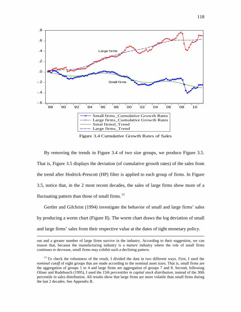
118
By removing the trends in Figure 3.4 of two size groups, we produce Figure 3.5.
That is, Figure 3.5 displays the deviation (of cumulative growth rates) of the sales from
the trend after Hodrick-Prescott (HP) filter is applied to each group of firms. In Figure
3.5, notice that, in the 2 most recent decades, the sales of large firms show more of a
fluctuating pattern than those of small firms.13
Gertler and Gilchrist (1994) investigate the behavior of small and large firms’ sales
by producing a worm chart (Figure II). The worm chart draws the log deviation of small
and large firms’ sales from their respective value at the dates of tight monetary policy. out and a greater number of large firms survive in the industry. According to their suggestion, we can reason that, because the manufacturing industry is a mature industry where the role of small firms continues to decrease, small firms may exhibit such a declining pattern.
13 To check the robustness of the result, I divided the data in two different ways. First, I used the nominal cutoff of eight groups that are made according to the nominal asset sizes. That is, small firms are the aggregation of groups 1 to 4 and large firms are aggregation of groups 7 and 8. Second, following Oliner and Rudebusch (1995), I used the 15th percentiles in capital stock distribution, instead of the 30th percentile in sales distribution. All results show that large firms are more volatile than small firms during the last 2 decades. See Appendix B.
-.6
-.4
-.2
.0
.2
.4
.6
.8
88 90 92 94 96 98 00 02 04 06 08 10
Small firms_Cumulative Growth RatesLarge firms_Cumulative Growth RatesSmal firmsl_TrendLarge firms_Trend
Figure 3.4 Cumulative Growth Rates of Sales
Small firms
Large firms

119
Chari, Christiano, and Kehoe (2007) reproduce Gertler and Gilchrist’s (1994) worm
chart, employing a business cycle shock instead of a monetary policy shock. Following
the method of Gertler and Gilchrist (1994) and Chari, Christiano, and Kehoe (2007), I
investigate the sales of small and large firms after either a business cycle shock or a
monetary policy shock. Therefore, the cumulative growth rates of small and large firms’
sales in Figure 3.5 are normalized by zero at the date of a monetary policy shock or at
the date of a business cycle peak. Then, we can produce a worm chart in the same
manner as previous research.
Figure 3.6 shows the sales of small and large firms after NBER recession shocks of
recent periods: 1990 Q3, 2001 Q1, and 2007 Q4. The vertical axis indicates the
cumulative growth rates of sales, and the horizontal axis indicates the time periods.
After an NBER recession shock, on average, the sales of large firms reduce
substantially more
-.20
-.16
-.12
-.08
-.04
.00
.04
.08
.12
.16
88 90 92 94 96 98 00 02 04 06 08 10
Small firms Large firms
Figure 3.5 Cumulative Growth Rates of Sales after HP Filtering
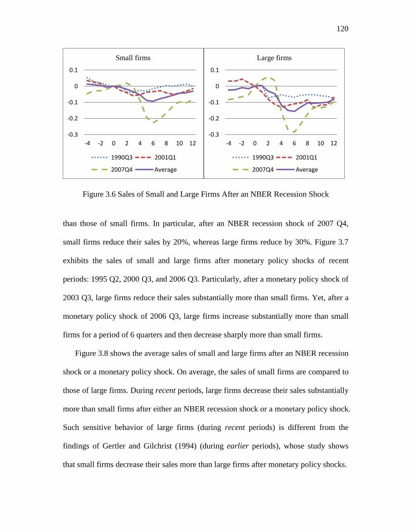
120
Figure 3.6 Sales of Small and Large Firms After an NBER Recession Shock
than those of small firms. In particular, after an NBER recession shock of 2007 Q4,
small firms reduce their sales by 20%, whereas large firms reduce by 30%. Figure 3.7
exhibits the sales of small and large firms after monetary policy shocks of recent
periods: 1995 Q2, 2000 Q3, and 2006 Q3. Particularly, after a monetary policy shock of
2003 Q3, large firms reduce their sales substantially more than small firms. Yet, after a
monetary policy shock of 2006 Q3, large firms increase substantially more than small
firms for a period of 6 quarters and then decrease sharply more than small firms.
Figure 3.8 shows the average sales of small and large firms after an NBER recession
shock or a monetary policy shock. On average, the sales of small firms are compared to
those of large firms. During recent periods, large firms decrease their sales substantially
more than small firms after either an NBER recession shock or a monetary policy shock.
Such sensitive behavior of large firms (during recent periods) is different from the
findings of Gertler and Gilchrist (1994) (during earlier periods), whose study shows
that small firms decrease their sales more than large firms after monetary policy shocks.
-0.3
-0.2
-0.1
0
0.1
-4 -2 0 2 4 6 8 10 12
Small firms
1990Q3 2001Q1
2007Q4 Average
-0.3
-0.2
-0.1
0
0.1
-4 -2 0 2 4 6 8 10 12
Large firms
1990Q3 2001Q1
2007Q4 Average

121
Figure 3.7 Sales of Small and Large Firms After a Monetary Policy Shock (Adrian Dates)
Figure 3.8 Average Sales of Small and Large Firms After Either an NBER Recession Shock or a Monetary Policy Shock
-0.3
-0.2
-0.1
0
0.1
-4 -2 0 2 4 6 8 10 12
Small firms
1995Q2 2000Q3
2006Q3 Average
-0.3
-0.2
-0.1
0
0.1
-4 -2 0 2 4 6 8 10 12
Large firms
1995Q2 2000Q3
2006Q3 Average
-0.2
-0.1
0
0.1
-4 -2 0 2 4 6 8 10 12
After NBER Recession Shocks
Small Large
-0.2
-0.1
0
0.1
-4 -2 0 2 4 6 8 10 12
After Monetary Policy Shocks
Small Large

122
3.4 Empirical Results
This section examines the behavior of the aggregate data in some balance sheet
variables (sales, inventories, trade debt, and total short-term debt) and the behavior of
the components of aggregate debt (bank debt, mortgages, commercial papers and other
debt). 14, 15 By using these variables, the behavior of small and large firms is explored by
different episodes, business cycle episodes and monetary policy episodes, and by
different periods, earlier periods and recent periods.
I report empirical results by different episodes. Empirical results of each episode
cover the comparison of small and large firms’ behavior between earlier periods (1960
Q1─1989 Q4) and recent periods (1990 Q1─2011 Q3).16 In particular, the comparison
of these two periods is made based on the flow of funds data because only the flow of
funds data are available for this long historical time period (1960 Q1─2011 Q3) among
four data sets described in Section 2―the flow of funds data, the QFR data, the SLOOS
data, and BED data.
3.4.1 The Responses of Small Versus Large Firms to the NBER Recessions
I examine the behavior of small and large firms during business cycle episodes by
using four different sources of data: the flow of funds data, the Quarterly Finance
14 Total short-term debt includes short-term bank debt, commercial papers, and short-term other debt
excluding trade debt. 15 The QFR data provide the components of short-term debt (i.e., short-term bank debt, commercial
paper, and short-term other debt) and component of long-term debt (i.e., long-term bank debt and long-term other debt), while the flow of funds data provide only components of aggregate debt without the distinction between short-term and long-term debt (i.e., bank debt, mortgages, commercial papers and other debt).
16 Earlier periods start in 1960 Q1 because the data for total short-term debt are only available from
1960 Q1.

123
Report (QFR) data, the Senior Loan Officer Opinion Survey (SLOOS) data, and the
Business Employment Dynamics (BED) data. The results are reported in the order of
data sets.
3.4.1.1 The Flow of Funds Data and the QFR Data
Employing the flow of funds data and the QFR data, Figure 3.9 shows the average
changes in some balance sheet variables and in components of aggregate debt after an
NBER recession shock. In particular, Figure 3.9 exhibits the outcome of the same
exercise of the previous Figure 3.6 and 3.7 in terms of some balance sheet variables and
the components of aggregate debt. For parsimony, I report only the average behavior of
small and large firms after an NBER recession shock, as in Figure 3.8.
Employing the flow of funds data, the first two columns in Figure 3.9 show the
average behavior of small and large firms during earlier periods (pre-1990 periods) and
recent periods (post-1990 periods). Employing the QFR data, the third column shows
the average behavior of small and large firms during recent periods (post-1990 periods).
I report partly the results of “sales,” “short-term bank debt,” and “mortgages” because
these variable are available only either for the flow of fund data or for the QFR data.
During recent periods in the QFR data (the third column), the sales of large firms
decrease drastically more than those of small firms after an NBER recession shock. For
a period of 6 quarters after an NBER recession shock, the sales of large firms decline by
roughly 15%, but small firms decline by roughly 10%. During earlier periods in the
flow of funds data (the first column), the inventories of small and large firms show
somewhat different responses after an NBER recession shock. Large firms tend to
decrease their inventories more slowly than small firms after an NBER recession shock.

124
F
low
of F
unds
Dat
a
Flow
of F
unds
Dat
a
Q
FR D
ata
(
Earli
er p
erio
ds: 1
960Q
1−19
89Q
4)
(Rec
ent P
erio
ds: 1
990Q
1−20
11Q
3)
(R
ecen
t Per
iods
: 199
0Q1−
2011
Q3)
Figu
re 3
.9 A
vera
ge C
hang
es in
Sal
es a
nd S
ome
Bal
ance
She
et V
aria
bles
Afte
r an
NB
ER R
eces
sion
Sho
ck

125
Fl
ow o
f Fun
ds D
ata
Fl
ow o
f Fun
ds D
ata
QFR
Dat
a
(Ear
lier p
erio
ds: 1
960Q
1−19
89Q
4)
(Rec
ent P
erio
ds: 1
990Q
1−20
11Q
3)
(R
ecen
t Per
iods
: 199
0Q1−
2011
Q3)
Fi
gure
3.9
Con
tinue
d

126
Flo
w o
f Fun
ds D
ata
Fl
ow o
f Fun
ds D
ata
QFR
Dat
a
(Ear
lier p
erio
ds: 1
960Q
1−19
89Q
4)
(Rec
ent P
erio
ds: 1
990Q
1−20
11Q
3)
(R
ecen
t Per
iods
: 199
0Q1−
2011
Q3)
Figu
re 3
.9 C
ontin
ued

127
Flo
w o
f Fun
ds D
ata
Fl
ow o
f Fun
ds D
ata
QFR
Dat
a
(Ear
lier p
erio
ds: 1
960Q
1−19
89Q
4)
(Rec
ent P
erio
ds: 1
990Q
1−20
11Q
3)
(R
ecen
t Per
iods
: 199
0Q1−
2011
Q3)
Figu
re 3
.9 C
ontin
ued

128
a similar way by less than 10 percent. Yet, during recent periods in the flow of fun
Flo
w o
f Fun
ds D
ata
Fl
ow o
f Fun
ds D
ata
QFR
Dat
a
(Ear
lier p
erio
ds: 1
960Q
1−19
89Q
4)
(Rec
ent P
erio
ds: 1
990Q
1−20
11Q
3)
(R
ecen
t Per
iods
: 199
0Q1−
2011
Q3)
Figu
re 3
.9 C
ontin
ued

129
However, during recent periods in the flow of funds and the QFR data (second and third
columns), the inventories of small and large firms show almost the same responses after
an NBER recession shock. For a period of 6 quarters after an NBER recession shock,
both small and large firms decrease their inventories by roughly 10%.
During earlier periods in the flow of funds data (the first column), the total short-
term debt of small and large firms exhibits somewhat similar responses after an NBER
recession shock. Both small and large firms slowly decrease their total short-term debt
in a similar way by less than 10%. Yet, during recent periods in the flow of funds and
the QFR data (the second and third columns), the total short-term debt of large firms
drops substantially more than that of small firms. In particular, in the flow of funds data,
large firms reduce their total short-term debt by roughly 18% for a period of 10 quarters
after an NBER recession, but small firms reduce it by 10%. Such substantial reduction
of short-term debt in large firms is more pronounced in the QFR data than in the flow of
funds data. In the QFR data, large firms decline their total short-term debt by roughly
25% for a period of 10 quarters after an NBER recession shock, but small firms reduce
it by roughly 5%.17
The components of aggregate debt exhibit a similar pattern to total short-term debt,
depending on different time periods. During earlier periods, both small and large firms
reduce total short-term debt comparably, whereas during recent periods, large firms
reduce total short-term debt substantially more than small firms. Likewise, during
earlier periods, both small and large firms, in general, similarly reduce the components
17 During recent periods, such substantial reduction of large firms is more clearly shown in short-
term bank debt of the QFR data. Large firms decrease short-term bank debt by about 45%, but small firms decrease by about 10%.

130
of aggregate debt, while during recent periods, large firms reduce the components of
aggregate debt substantially more than small firms.
During earlier periods in the flow of funds data (the first column), the components
of aggregate debt show somewhat similar responses after an NBER recession shock.
The bank debt of small firms decreases slightly more than that of large firms; the
mortgages and other debt of small firms decrease slightly less than those of large firms.
However, during recent periods in the flow of funds data and the QFR data (the second
and third column), the components of short-term debt shows that the bank loans,
mortgages and other debt of large firms―except the other debt of the QFR
data―decrease substantially more than those of small firms after an NBER recession.
When the components of aggregate debt during earlier periods are compared to
those during recent periods in the flow of funds data (the first and second columns), the
bank loan, mortgages, commercial papers, and other debt of large firms during recent
periods (the second column) decrease substantially more than those of large firms
during earlier periods (the first column). In particular, the commercial papers of large
firms decrease during recent periods considerably more than during earlier periods. For
a period of 8 quarters after an NBER recession shock, large firms reduce the
commercial papers by around 5% during earlier periods, but reduce them by around 35%
during recent periods.
During recent periods (the second and third columns), when the flow of funds data
are compared to the QFR data for all applicable variables, all variables except other
debt (i.e., inventories, total short-term debt, bank debt, commercial and trade debt)
display similar results. Generally, large firms reduce these variables significantly more

131
than small firms. The other debt of small firms shows somewhat different behavior
between the flow of funds and the QFR data.18 The trade debt of large firms decreases
more than that of small firms in all datasets and in all different periods (the first, second,
and third columns).
The main finding is that during recent periods, in general, some balance sheet
variables and components of aggregate debt in large firms decrease substantially more
than those of small firms after an NBER recession shock. In particular, total short-term
debt reflects this phenomenon very well. The declining pattern of total short-term debt
in large firms is more pronounced in the QFR data than in the flow of funds data.
3.4.1.2 The Senior Loan Officer Opinion Survey Data
The Senior Loan Officer Opinion Survey (SLOOS) data are other sources of data
we can use to examine the behavior of small and large firms. As stated in Section 2, the
Federal Reserve conducts surveys to find out how the senior loan officers (at each
respondent banks) feel about their lending practices―such as changes in the standards
and terms of bank loans―in the credit market over the past 3 months. For the questions
that examine banks’ lending standards and banks’ lending terms,19 respondents (i.e.,
18 The different behavior of other debt in small firms―between the flow of funds and the QFR data
during recent periods―may result from the somewhat different characteristics of other debt in each set of the flow of funds and the QFR data. Other debt is defined as the residual of total debt after subtracting the components of debt from the total debt in each set of data. Because the components of debt in the flow of fund data are different from those in the QFR, other debt in the flow of funds data is different from that in the QFR data. In the flow of funds, other debt includes foreign debt, debt from saving institutions and credit unions, finance companies and so on (Federal Reserve, 2000). However, short-term other debt in the QFR data includes mortgages, nonbank financial institutions’ debt, and so forth. Notice that mortgages are categorized as other debt in the QFR, whereas they are not categorized as other debt in the flow of funds data.
19 To reiterate, the question about banks’ lending standards is “How have your credit standards for
C&I loans to small firms and large and medium-size firms changed over the past 3 months?” The question about banks’ lending terms is “How have the terms of C&I loans to small firms and large and

132
senior loan officers at banks) can answer the questions with one of the five given
choices: (1) Tightened considerably, (2) tightened somewhat, (3) remained basically
unchanged, (4) eased somewhat, and (5) eased considerably. Also, for the question
about the state of business demand for loans,20 respondents can answer the questions
with one of the five given options: (1) Substantially stronger, (2) moderately stronger,
(3) about the same, (4) moderately weaker, and (5) substantially weaker.
Figure 3.10 shows the net percentage of domestic respondents that report a
tightening of loan standards for commercial and industrial (C&I) loans. The net
percentage tightening here is defined as the number of loan officers reporting tightening
standards (“tightened considerably” or “tightened somewhat”) minus the number
medium-sized firms―with respect to spread of loan rates over banks’ costs of funds―changed over the past 3 months?”
20 The question about the state of business demand for loans is “Apart from normal seasonal
variation, how has demand for C&I loans from large and medium-size firms and small firms changed over the past 3 months?”
-40
-20
0
20
40
60
80
100
90 92 94 96 98 00 02 04 06 08 10 12
Small firmsLarge and medium-size firms
Figure 3.10 Net Percentage of Domestic RespondentsTightening Standards for C&I Loans
Shaded areas indicate the NBER recessions

133
reporting easing (“eased considerably” or “eased somewhat”) divided by the total
number reporting. Although a tightening of loan standards in “small firms” and “large
and medium-size firms” tends to rise and fall in a similar way over the sample periods,
senior loan officers report that they increase their loan standards to large and medium-
size firms more than to small firms during all three NBER recessions. In particular,
during the 2001 recession, banks increased their standards to large and medium-size
firms substantially more than to small firms. Yet, during the recessions of 1990 to 1991
and of 2007 to 2009, they increased to large and medium-size firms slightly more than
to small firms.
Figure 3.11 shows the net percentage of domestic respondents that report an
increase in loan spreads between loan rates and banks’ cost of funds for C&I loans. A
wider spread of loan rates over cost of funds indicates that a bank tightens its lending
practices, and a narrower spread indicates that a bank eases its lending practices.
-80
-40
0
40
80
120
90 92 94 96 98 00 02 04 06 08 10 12
Small firmsLarge and medium-size firms
Figure 3.11 Net Percentage of Domestic Respondents IncreasingSpreads of Loan Rates over Banks' Cost of Funds
Shaded areas indicate the NBER recessions

134
Similarly, the net percentage spreads are defined as the number of loan officers
reporting an increase in loan spreads (“tightened considerably” or “tightened
somewhat”) minus the number reporting an decrease in loan spreads (“eased
considerably” or “eased somewhat”) divided by the total number reporting. Increases or
decreases in loan spreads to large and medium-size firms are noticeably more volatile
than the correspondence to small firms over the business cycles. Such different
fluctuations suggest that during a contraction, banks increase their loan spreads to large
and medium-size firms substantially more than to small firms; during an expansion,
they also decrease to large and medium-size firms significantly more than to small
firms. While banks increased very similarly their loan spreads between these two kinds
of firms during the recession of 2007 to 2009, they nevertheless increased their loan
spreads to large and medium-size firms considerably more than to small firms during
the recession of 1990 to 1991 and the 2001 recession.
Figure 3.12 shows the net percentage of domestic respondents that report a stronger
demand of businesses for C&I loans. Likewise, the net percentage demand is defined as
the number of loan officers reporting a stronger demand of business (“substantially
stronger” or “moderately stronger”) minus the number reporting a weaker demand of
business (“substantially weaker” or “moderately weaker”) divided by the total number
reporting. We can observe a similar pattern in loan demand of businesses from what
happen to the banks’ lending standards and terms. A stronger loan demand to large and
medium-size firms tends to fluctuate more than the equivalence to small firms over the
sample periods. Such variations suggest that during a contraction, large and medium-
size firms increase their demand for credit more than small firms; during an expansion,

135
they decrease their demand for credit more than small firms. In particular, banks
perceive that “small firms” and “large and medium-size firms” decrease very
comparably their demand during the recession of 2007 to 2009, but banks perceive that
large and medium-size firms decrease their demand significantly more than small firms
during the 2001 recession―the data of the 1990 recession are not available in this net
percentage demand.
3.2.1.3 The Business Employment Dynamics Data
The BED data also can be used to examine the behavior of small and large firms in
terms of employment. Although Birch (1979) finds that small businesses account for a
particularly large share of new jobs created in the U.S economy (reporting that
establishments with 100 or fewer employees create 81.5% of net new jobs between
1960 and 1976), a number of researchers cast doubt on his finding. They suggest that
-80
-60
-40
-20
0
20
40
60
90 92 94 96 98 00 02 04 06 08 10 12
Small firmsLarge and medium-size firms
Figure 3.12 Net Percentage of Domestic RespondentsReporting Stronger Demand for C&I Loans
Shaded areas indicate the NBER recessions

136
his finding is somewhat overestimated for the role of small firms in job creation.
Armington and Odle (1982) find that, when they classify business sizes by the number
of employees working for firms (i.e., a firm basis) rather than the number of employees
working at each location (i.e., an establishment basis), 21 firms with 100 or fewer
employees generate only 39% of net jobs between 1978 and 1980. Brown, Hamilton,
and Medoff (1990) find that 40% of jobs possessed by small businesses in 1980 had
disappeared after 6 years, which implies that small businesses tend to produce short-
lived jobs. They claim that small businesses are not responsible for such a large share of
jobs when we pay attention to jobs that are not short-lived. Furthermore, Davis,
Haltiwanger, and Schuh (1998) criticize Birch’s methodology of classifying businesses
into size categories because Birch’s approach produces an upward bias in the
contribution of small firms to job growth. They point out that, when Birch uses base-
year employment in the denominator in the calculation of job growth rate, the base-year
employment leads to a statistical pitfall, which indicates that employment growth is
stemming from small firms. This is known as the “regression fallacy” or “regression-to-
the-mean” bias.
To deal with some of the problems described above, the BED begins providing the
data of business size categories in a different way. Business sizes are classified by the
firm level (instead of the establishment level), and an alternative method, known as “a
dynamic-sizing method,” is used (instead of the base-year method) when the BED
classifies businesses into size classes. In addition to providing more accurate data, the
21 “An establishment is typically defined as an economic unit, such as a factory or store, which
produces goods and provides services. An establishment is a physical location and is engaged in one, or predominantly one, type of economic activity. In contrast, a firm is defined as an aggregation of establishment under common ownership by a corporation parent” (Okolie, 2004, p. 4).
137
BED also provides the decomposition data of net employment growth, which allow us
to understand the dynamics of the job market in more depth. In the quarterly BED data
series, the net employment change is decomposed mainly into “gross job gains” and
“gross job losses.” Gross job gains are divided furthermore into business openings and
expansions. Gross job losses are divided additionally into business closings and
contractions.
Based on the BED data from 1992 Q2 to 2011 Q4, Table 3.1 displays the quarterly
average of gross job gains, gross job losses, and net changes by firm sizes. The job
gains, job losses, and net changes are reported basically in three different ways: level
(panel A), share (panel B), and growth rate (panel C). As shown in panel A, the
employment level data show that the economy, on average, created a total of 251,000
jobs each quarter over the sample periods. Such employment increase is the net result of
two factors: the jobs created by business openings and expansions and the jobs lost by
business closings and contractions. Opening and expanding businesses created an
average of 6.3 million jobs each quarter, whereas closing and contracting businesses
lost an average of 6.1 million jobs. Each of these figures is much large than the net
employment figures, 251,000. These statistics indicate the substantial number of job
churning that happens in the U.S economy every quarter.
More specifically, as to gross job gains, employment expanding businesses
increased by an average of 5.3 million jobs per quarter, and employment opening
businesses increased by an average of 1 million jobs. Expanding businesses,
consequently, account for about 84% of gross job gains each quarter (5.3 million
jobs/6.3 million jobs), and opening businesses account for remaining about 16% (1

138
Table 3.1 Average Quarterly Level, Share, and Growth Rate of Gross Job Gains and Gross Job Losses by Firm Size (seasonally adjusted, 1992 Q3 to 2011 Q4) Size Classes (Number of Employees)
Categories
(1) 1 to 4
(2) 5 to 9
(3) 10 to 19
(4) 20 to 49
(5) 50 to 99
(6) 100 to 249
(7) 250 to 499
(8) 500 to 999
(9) 1000 or more
(10) Total
(11) Aver -age
A. Level (in Thousand)
Gross Job Gains 944 739 761 904 572 612 369 302 1,130 6,333 ―
Expansions 379 573 643 809 533 586 359 296 1,122 5,301 ―
Openings. 565 166 117 95 39 26 10 6 8 1,032 ―
Gross Job Losses 925 727 743 874 547 578 347 285 1,058 6,082 ―
Contractions 389 569 630 779 505 546 333 276 1,049 5,075 ―
Closings 536 158 113 95 42 32 14 8 10 1,007 ―
Net Change 19 13 18 30 25 34 22 17 72 251 ―
B. Share (Percent of the Categories) 1
Gross Job Gains 15 12 12 14 9 10 6 5 18 100 ―
Expansions 7 11 12 15 10 11 7 6 21 100 ―
Openings 55 16 11 9 4 3 1 1 1 100 ―
Gross Job Losses 15 12 12 14 9 9 6 5 17 100 ―
Contractions 8 11 12 15 10 11 7 5 21 100 ―
Closings 53 16 11 9 4 3 1 1 1 100 ―
Net Change 8 5 7 12 10 14 9 7 29 100 ― Cumulative Share of Net Change 8 13 20 32 42 56 64 71 100 ― ―
C. Growth Rate (Percent of Total Employment) 2
Gross Job Gains 17.3 11.3 9.4 7.7 6.5 5.5 4.8 4.2 2.9 ― 7.7
Expansions 6.9 8.8 7.9 6.9 6 5.3 4.7 4.1 2.9 ― 5.9
Openings 10.3 2.5 1.4 0.8 0.4 0.2 0.1 0.1 0 ― 1.8
Gross Job Losses 16.8 11.1 9.1 7.4 6.1 5.1 4.5 3.9 2.7 ― 7.4
Contractions 7.1 8.7 7.7 6.6 5.7 4.9 4.3 3.8 2.6 ― 5.7
Closings 9.8 2.4 1.4 0.8 0.5 0.3 0.2 0.1 0 ― 1.7
Net Change 0.4 0.2 0.3 0.3 0.3 0.4 0.3 0.3 0.2 ― 0.3
1 Share measures the percent of the categories―i.e., gross job gains, expansions, contractions etc.― represented by each firm class. 2 Growth rate measures the gross job gains, gross job losses, expansions, openings, contractions and openings as a percentage of average of the previous and current total employment. †Source: An author' calculations based on Bureau of Labor Statistics' Business Employment Dynamics dataset. Some percentages do not total 100 due to rounding.

139
million jobs/6.3 million jobs)―on average over the sample period. On the other hand,
regarding gross job losses, employment contracting businesses decreased by an average
of 5.1 million jobs, and employment closing businesses decreased by an average of 1
million jobs. Contracting businesses, hence, account for about 84% of gross job losses,
and closing businesses account for the residual about 16%―on average over the sample
period. These statistics indicate that it is expanding and contracting businesses that
constitute a majority of gross job gains and losses in the labor market, not opening and
closing businesses.
As previously reported, the economy has experienced gross job gains, averaging a
gain of 6.3 million jobs each quarter. A natural question arises: “Which firm size group
accounts for the most job gains?” Panel B answers this question. Firms with fewer than
50 employees contributed an average of 53% of gross job gains (15+12+12+14), and
firms with fewer than 100 employees contributed 62% (53+9). On the other hand, the
economy has experienced gross job losses, averaging a loss of 6.1 million jobs each
quarter. Firms with fewer than 50 employees had a 53% share of gross job losses
(15+12+12+14), and firms with fewer than 100 employees had a 62% share of gross job
losses (53+9). Subtracting gross job losses from gross job gains produces an average net
gain of 251,000 jobs. Firms with fewer than 50 employees contributed about 32% of
average net job change, and firms with fewer than 100 employees contributed 42%. To
understand whether small firms create more jobs than large firms, it is required to
compare the share of small firms in total job creation to the share of their total
employment. The comparison of these two shares reveals that the share of these firms in
total job creation is greater than the share of their total employment. Firms with fewer

140
than 50 employees made up 30% of total employment (but contributed 32% of net job
creation), and firms with fewer than 100 employees made up 37% (but contributed
42%)―the share of total employment is not shown in Table 3.1. 22 These statistics
suggest that small firms contributed a larger share of new jobs over the past 2
decades23―nonetheless, a larger share of their new jobs is still open to question over
the phase of the business cycle, especially during a recession.
The very large firms, those with 1000 or more employees, made up 18% of gross
job gains, the highest share among the nine size firms. The next largest share appears
with the size class 1 to 4 employees, with 15% of gross job gains. These two size
groups also had the largest quarterly share of gross job losses, 17% and 15%,
respectively. The business openings and closings took place mostly in smaller size
groups. In the size class of 1 to 4 employees, the average share of gross job gains was
55% each quarter, and the average share of gross job losses was 53%. Notice that this
share decreases as firm size increases.
As shown in panel C, the growth rates show that the economy has experienced
about 7.7% of average gross job gain rate and about 7.4% of average gross job loss rate
over the sample periods. These figures mean that the jobs created by opening and
expanding businesses account for average 7.7% of the total number of jobs during a
quarter; similarly, the job lost by closing and contracting businesses comprise average
22 The share of total employment (not shown in Table 3.1) is based on the establishment level, not the
firm level, from the data of Business Dynamic Statistics (BDS). 23 Brown et al. (1990) suggest that we should not conclude from this result―the larger contribution
of small firms to new jobs―that small firms grow faster than larger ones. Indeed, the mortality rate for small firms is much higher than that of large firms. Such high mortality rate influences the faster growth rates of small firms among survivors. “If calculation [of growth rate] is extended to include all firms existing in the initial year, and not just those that survived, small businesses declined faster than large ones” (p. 24).

141
7.4% of total number of jobs. The difference of 3% between these two statistics is an
average of net employment growth rate during a quarter. In this analysis, we will pay
special attention to the net employment growth measured as a rate, rather than an
employment level, because using an employment growth rate permits us to compare
changes in the behavior of small and large firms more reasonably. To understand better
the underlying dynamics of the net employment growth rate, we need to turn to the
components of the net employment growth measured as rates―a gross job gains rate
and a gross job losses rate.
Figure 3.13 shows gross job gain (job creation) rates and gross job loss (job
destruction) rates between small and larger firms. In this graph, small firms are defined
as firms with 1 to 49 employees, and large firms are defined as those with 50 or
more.24, 25 Over the past 2 decades, we can see a striking difference of job creation rates
and destruction rates between small and large firms. Both the job creation rates and job
destruction rates of small firms are very high, ranging from 9 to 13%. In contrast, these
two statistics of large firms are somewhat low, ranging from 3 to 6%. Such a different
tendency suggests that small firms create and also destruct jobs at a fast rate, while large
firms create and also destruct jobs at a slow rate.26 Because an important statistic we
24 I report only the results produced by this definition of small and large firms because other two definitions―which indicate small firms as those with 1 to 99 employees and those with 1 to 499 employees―produce similar results.
25 Job gain rates are measured by averaging the job gain rates of each size classes of small and large
firms according to the definition of each group of firms. For example, when small firms are defined firms with 1 to 49, I first calculate the job gain rates of each of the first four size classes. Then, I divide the sum of the job gain rates of these four size classes by 4, i.e., (the rate of size class 1 + of size class 2 + of size class 3 + of size class 4)/4.
26 Although I did not report expansion rates, contraction rates, opening rates, and closing rates, the behavior of these components reflects a pattern of job creation rates and job destruction rates between small and large firms. That is, existing small firms tend to expand and contract jobs at the higher rate than

142
must focus on is the difference between job creation rates and destruction rates, this
leads us to investigate net job creation rates, a more accurate measure of job creation in
the economy.
Figure 3.14 shows the behavior of both the net job creation (levels) and the net job
creation rate between small and large firms from 1992 Q3 to 2011 Q4. To examine the
behavior of small and large firms more thoroughly in terms of net job creation, small
and larger firms are defined in three different ways, as stated in Section 2: (1) small
firms are a group that hires 1 to 49 employees, and larger firms are a group that hires 50
or more employees; (2) small firms are a group that hires 1 to 99 employees, and larger
firms are a group that hires 100 or more employees; and (3) small firms are a group that
hires 1 to 499 employees, and larger firms are a group that hires 500 or more employees.
existing large firms do; small firms tend to open and close their businesses at a greater rate than large firms do.
2
4
6
8
10
12
14
1992 1994 1996 1998 2000 2002 2004 2006 2008 2010
1 to 49: Gross Job Gain Rate1 to 49: Gross Job Loss Rate50 or more: Gross Job Gain Rate50 or more: Gross Job Loss Rate
Figure 3.13 Gross Job Gain Rates and Gross Job Loss Rates
Shaded areas indicates the NBER recessions.

143
Pane
l A: N
et Jo
b Cr
eatio
n (in
Tho
usan
d)
Pane
l B: N
et Jo
b Cr
eatio
n R
ates
afte
r HP
Filte
ring
from
Cum
ulat
ive
Gro
wth
Rat
e (P
erce
nt)
Figu
re 3
.14
Net
Job
Cre
atio
n an
d N
et Jo
b C
reat
ion
Rat
es B
etw
een
Smal
l and
Lar
ger F
irms,
1992
Q3
to 2
011
Q4

144
Panel A in Figure 3.14 displays the “net job creation” measured as an employment
level. In the first two definitions of small and large firms (the first two columns), the net
job creation of larger firms is more volatile than that of small firms during 2001
recession and the 2007-2009 recession. Yet, in the third definition (the third column),
the situation is reversed; the net job creation of small firms is more variable than that of
large firms, particularly when we look at the 2007-2009 recession. This is partly
because, I believe, when the net job creation is measured by the employment level, the
fluctuations of small firms tend to change depending on how we classify small firms.
For example, if small firms are defined to include more firm size classes, they are likely
to show more net change in employment levels due to an increase in their population.
To address this issue, panel B in Figure 3.14 displays net job creation rates, rather
than the employment level. Net job creation rates compare the contribution of job
creation between small and large firms more accurately because they show a portion of
the total number of jobs. As in Section 2, the growth rates of net job creation are
reported hereafter I remove a trend from cumulative growth rates by using Hodric-
Prescott (HP) filter. Notice that, when net job creation rates are used in panel B, the
difference of the behavior between small and large firms is less dramatic than when the
net job creation (levels) are used in panel A. During the 2001 recession, the net job
creation rates of larger firms are somewhat more volatile than those of small firms in all
three definitions of small and large firms. Yet, during the 2007-2009 recession, the net
job creation rates of small firms are slightly more variable than those of larger firms in
all three definitions. To examine the behavior of small and large firm between the 2001

145
and the 2007-2008 recessions more closely, the cumulative growth rates of net job
creation are normalized by zero at the start date of the NBER recession, as in Section 2.
Figure 3.15 shows that, during the 2001 recession, the net job creation of large firms
decreased substantially more than that of small firms in all three definitions (the left
three columns). These results are consistent with the results produced from the SLOOS
data set. Remember that senior loan officers report that, during the 2001 recession, they
increased their loan standards and loan spreads to large and medium-size firms
substantially more than to small firms (Figure 3.10 and 3.11) and that they also
perceived large and medium-size firms increase their loan demand significantly more
than small firms (Figure 3.12). On the other hand, during the 2007 to 2009 recession,
the net job creation of small firms declines almost to the same extent as that of large
firms (the first two columns in the right) or decrease slightly more than that of large
firms (the bottom right column). These outcomes are also generally consistent with the
outcomes produced from the SLOOS data. Recall that senior loan officers report that,
during the 2007-2009 recession, they increased their loan standards and loan spreads to
a very similar degree between small and large and medium-size firms or increased these
two elements to large and medium-size firms slightly more than small firms (Figure
3.10 and 3.11), and that they see these two kinds of firms decrease their loan demand to
almost the same extent (Figure 3.12).

146
The 2001 Recession The Recession of 2007 to 2009
Figure 3.15 Cumulative Employment Changes Since the Start of the 2001 and
2007-2009 Recessions
-5-4-3-2-1012
2000Q1
2001Q1
2002Q1
2003Q1
2004Q1
1 to 49 50 or more
-5-4-3-2-1012
2006Q4
2007Q4
2008Q4
2009Q4
2010Q4
1 to 49 50 or more
-5-4-3-2-1012
2000Q1
2001Q1
2002Q1
2003Q1
2004Q1
1 to 99 100 or more
-5
-4
-3
-2
-1
0
1
2
2006Q4
2007Q4
2008Q4
2009Q4
2010Q4
1 to 99 100 or more
-5-4-3-2-1012
2000Q1
2001Q1
2002Q1
2003Q1
2004Q1
1 to 499 500 0or more
-5-4-3-2-1012
2006Q4
2007Q4
2008Q4
2009Q4
2010Q4
1 to 499 500 or more

147
3.4.2 The Responses of Small Versus Large Firms to Monetary Policy
3.4.2.1 The Flow of Funds Data and the QFR Data
I examine the behavior of small and large firms during monetary policy episodes by
using two different sources of data: the flow of funds data and the Quarterly Finance
Report (QFR) data. In this analysis, two types of monetary policy shocks―“Romer
dates” and “Adrian dates”―are used. As mentioned in Section 2, “Romer dates” are
available only for earlier periods (pre-1990 periods) while “Adrian dates” are available
for long historical sample periods (1960 Q1 – 2011 Q3). Although I have employed two
types of monetary policy shocks, only the results produced by using “Adrian dates” are
reported in this subsection. This is because “Adrian dates” allow us to make a
comparison between earlier periods and recent periods. Nonetheless, the results
produced by using “Romer dates” are also reported in Appendix C.
Employing the flow of funds data and the QFR data, Figure 3.16 shows the average
changes in some balance sheet variables (sales, inventories, trade debt and total short-
term debt) and in components of aggregate debt (bank debt, mortgages, commercial
papers, and other debt) after a tight monetary policy shock. I also report only the
average behavior of small and large firms after a tight monetary shock. Employing the
flow of funds data, the first two columns show the average behavior of small and large
firms during earlier periods (pre-1990 periods) and recent periods (post-1990 periods).
Employing the QFR data, the third column shows the average behavior of small and
large firms during recent periods (post-1990 periods). In addition, I report partly the
results of “sales,” “short-term bank debt,” and “mortgages” for either the flow of funds
data or the QFR data because these variables are available only for one of the two data

148
F
low
of F
unds
Dat
a
Flow
of F
unds
Dat
a
Q
FR D
ata
(E
arlie
r per
iods
: 196
0Q1−
1989
Q4)
(R
ecen
t Per
iods
: 199
0Q1−
2011
Q3)
(
Rec
ent P
erio
ds: 1
990Q
1−20
11Q
3)
Fi
gure
3.1
6 A
vera
ge C
hang
es in
Sal
es a
nd S
ome
Bal
ance
She
et V
aria
bles
Afte
r a M
onet
ary
Polic
y Sh
ock
(Adr
ian
Dat
e)

149
F
low
of F
unds
Dat
a
Flow
of F
unds
Dat
a
Q
FR D
ata
(E
arlie
r per
iods
: 196
0Q1−
1989
Q4)
(R
ecen
t Per
iods
: 199
0Q1−
2011
Q3)
(
Rec
ent P
erio
ds: 1
990Q
1−20
11Q
3)
Fi
gure
3.1
6 C
ontin
ued

150
F
low
of F
unds
Dat
a
Flow
of F
unds
Dat
a
Q
FR D
ata
(E
arlie
r per
iods
: 196
0Q1−
1989
Q4)
(R
ecen
t Per
iods
: 199
0Q1−
2011
Q3)
(
Rec
ent P
erio
ds: 1
990Q
1−20
11Q
3)
Fi
gure
3.1
6 C
ontin
ued

151
F
low
of F
unds
Dat
a
Flow
of F
unds
Dat
a
Q
FR D
ata
(E
arlie
r per
iods
: 196
0Q1−
1989
Q4)
(R
ecen
t Per
iods
: 199
0Q1−
2011
Q3)
(
Rec
ent P
erio
ds: 1
990Q
1−20
11Q
3)
Fi
gure
3.1
6 C
ontin
ued

152
F
low
of F
unds
Dat
a
Flow
of F
unds
Dat
a
Q
FR D
ata
(E
arlie
r per
iods
: 196
0Q1−
1989
Q4)
(R
ecen
t Per
iods
: 199
0Q1−
2011
Q3)
(
Rec
ent P
erio
ds: 1
990Q
1−20
11Q
3)
Figu
re 3
.16
Con
tinue
d

153
sets.
During recent periods in the QFR data (the third column), the sales of small firms
hover around zero up to 8 quarters after a monetary policy shock and afterward start to
decline; the sales of large firms begin to decline slightly after a monetary policy shock
and then recover until 8 quarters have passed. Finally, they decline sharply. In
particular, the sales of small and large firms in Figure 3.16 exhibit a very similar pattern
to the sales of small and large firms in Figure 3.9, which are produced after an NBER
recession shock. Just as large firms decrease sales substantially more than small firms
after an NBER recession shock, their sales decrease significantly more than small firms
after a monetary policy shock. However, a monetary policy shock has a weaker impact
on the sales of small and larger firms than an NBER recession shock. During earlier
periods in the flow of funds data (the first column), the inventories of small firms drop
slightly more than those of large firms. Yet, during recent periods in the flow of funds
and the QFR data (second and third columns), this pattern tends to change; large firms
decrease their inventories more than small firms.
During earlier periods in the flow of funds data (the first column), the total short-
term debt of small and large firms behaves similarly after a monetary policy shock,
showing virtually flat-shaped responses. Yet, during recent periods in the flow of funds
and the QFR data (the second and third column), both small and large firms tend to
increase their total short-term debt after a monetary policy shock. The total short-term
debt of small and large firms shows a rising-and-falling pattern (an inverse U shape)
during periods of tight monetary policy. This result is consistent with the results

154
produced from past research.27 In particular, recent periods of those two data sets reveal
that, after a monetary policy shock, large firms increase their total short-term debt
somewhat more than small firms. Such behavior of large firms is more pronounced in
the QFR data than in the flow of funds data.
The components of aggregate debt do not show a consistent pattern after a monetary
policy shock. During recent periods, bank debt and other debt of small and large firms
display a rising-and-falling pattern in the flow of fund data (the second column), but
they show an ambiguous behavior in the QFR data (the third column). Similarly, it is
very difficult to find a consistent pattern in the other components of aggregate debt.
During earlier periods in the flow of funds data (the first column), the trade debt of
large firms tends to decrease slightly more than that of small firms. During recent
periods in the flow of funds data (the second column), large firms decrease their trade
debt immediately after a monetary policy shock, but small firms are initially unaffected
and start to increase slightly after 5 quarters. During recent periods in the QFR data (the
27 Employing the QFR data, Gertler and Gilchrist (1994) find that after tightening monetary policy,
the behavior of total short-term debt mirrors the behavior of inventories for small and large firms. Following tight monetary policy, large firms tend to increase both inventories and total short-term debt, whereas small firms tend to decrease both inventories and total short-term debt. Gertler and Gilchrist interpreted these results as support for the notion that large firms may borrow total short-term debt more than small firms to smooth the impact of a recession―at the time that the need for external finances rises to carry inventory accumulations. Gertler and Gilchrist’s interpretation works well during earlier periods. In other words, the inventories and bank debt of large firms increase more than those of small firms during earlier periods in the flow of funds data (the first column).
Although Gertler and Gilchrist’s interpretation works well in the earlier-period flow of funds data, it
does not fit into the recent-period flow of funds and QFR data. During recent periods, I find that the short-term debt of large firms increases more than that of small firms, consistent with Gertler and Gilchrist’ (1994) findings. However, the inventories of large firms tend to decrease, not increase, whereas the inventories of small firms sharply increase or are unaffected for some periods. The question is “Why do large firms still increase total short-term debt in spite of a decrease in their inventories?” One possible explanation is that, since large firms experience the decline in sales (the first row) and thus a decline in cash flow, they may still need to borrow more short-term debt to finance operating costs rather than inventory costs.

155
third column), small and large firms show a similar response; they hover around zero
until 6 quarters and afterward begin to decline.
The main finding is that, during recent periods, the total short-term debt of small
and large firms tends to increase after a monetary policy shock. In particular, large firms
increase their total short-term debt more than small firms. Such behavior of large firms
is shown more clearly in the short-term bank debt of the QFR data. Moreover, during
recent periods, some balance sheet variables and components of debt of larger firms
generally show more sensitive behavior than those of small firms following a monetary
policy shock.
When the NBER recession episodes (in Figure 3.9) are compared to the tight
monetary episodes (in Figure 3.16), an NBER recession shock shows a substantially
stronger impact on the behavior of firms than a monetary policy shock. During the
NBER recession episodes, the behavior of firms is usually captured in the vertical axis
that ranges from 1 to –2. During tight monetary episodes, the behavior of firms is
typically captured in the vertical axis that ranges from 1 to –1. In addition, during recent
periods, when the flow of funds data are compared to the QFR data for the total short-
term debt and (short-term) bank debt, large firms show much more sensitive behavior
than small firms, as shown in Figure 3.9 and 3.16.
3.4.3 Is a Monetary Policy Shock Different from an NBER
Recession Shock?
Figure 3.17 and 3.18―which are extracted from Figure 3.9 and Figure 3.16,
respectively―show the average changes in “total short-term debt” and “short-term bank
debt” after either an NBER recession shock or a monetary policy shock. The

156
Flo
w o
f Fun
ds D
ata
Flo
w o
f Fun
ds D
ata
QFR
Dat
a
(E
arlie
r per
iods
: 196
0Q1−
1989
Q4)
(R
ecen
t Per
iods
: 199
0Q1−
2011
Q3)
(R
ecen
t Per
iods
: 199
0Q1−
2011
Q3)
Fi
gure
3.1
7 A
vera
ge C
hang
es in
Tot
al S
hort-
term
Deb
t and
Sho
rt-te
rm B
ank
Deb
t Aro
und
Beg
inni
ng D
ates
of
NB
ER R
eces
sion
s

157
Flo
w o
f Fun
ds D
ata
Fl
ow o
f Fun
ds D
ata
QFR
Dat
a
(Ear
lier p
erio
ds: 1
960Q
1−19
89Q
4)
(Rec
ent P
erio
ds: 1
990Q
1−20
11Q
3)
(R
ecen
t Per
iods
: 199
0Q1−
2011
Q3)
Fi
gure
3.1
8 A
vera
ge C
hang
es in
Tot
al S
hort-
term
Deb
t and
Sho
rt-te
rm B
ank
Deb
t Aro
und
Mon
etar
y Po
licy
Shoc
k
(Adr
ian
Dat
es)

158
comparison of these results suggests that a monetary policy shock is somewhat different
from an NBER recession shock in that it affects a short-term financing pattern of firms
differently in recent periods. As shown in Figure 3.17 and 3.18, in recent periods (the
second and the third column), both small and large firms tend to decrease total short-
term debt and short-term bank debt after an NBER recession shock, while they tend to
increase these debts after a monetary policy shock.28 In particular, it is important to
notice that large firms show much more sensitive behavior than small firms―after
either an NBER recession shock or a monetary policy shock. Large firms decrease
short-term bank debt substantially more than small firms after an NBER recession
shock; likewise, they increase short-term bank debt significantly more than small firms
after a monetary policy shock.
More specifically, by comparing the behavior of “the QFR data” to the behavior of
the “Flow of Funds data” (the second versus the third column), we can observe that the
excess sensitivity of large firms is more pronounced in the QFR data than in the flow of
funds data―after either an NBER recession shock or a monetary policy shock.
Furthermore, examining only the QFR (the third column) allows us to compare the
behavior of “total short-term debt” and the behavior of “short-term bank debt” after
each kind of shock―i.e., the comparison of the first and the second row in the third
column. It is interesting to note that such excess sensitivity of large firms is even more
pronounced in short-term bank debt than in total short-term debt. That is, after an
NBER recession shock, a comparison between the total short-term debt and the short-
term bank debt (in the third column of Figure 3.17) shows that, for large firms, the
28 In the earlier periods, on the other hand, either small or large firms are practically unaffected or
slightly decline total short-term debt and short-term bank debt after the two kinds of shocks.

159
trough of short-term bank debt is two times as deep as the trough of total short-term
debt: −0.45 in short-term bank debt and −0.27 in total short-term debt. On the other
hand, after a monetary policy shock, a comparison between total short-term debt and
short-term bank debt (in the third column of Figure 3.18) shows that, for large firms, the
peak of short term bank debt is four times as tall as the peak of total short-term debt:
0.27 for short-term bank debt and 0.07 for total short-term debt. From these empirical
results, several critical questions arise:
• Why do small and large firms tend to decrease total short-term debt and short-
term bank debt after an NBER recession shock?
• Why do small and large firms tend to increase total short-term debt and short-
term bank debt after a monetary policy shock?
• Furthermore, why do large firms show more sensitive responses (than small
firms) to either an NBER recession shock or a monetary policy shock in recent
periods?
This research paper provides some responses to these three questions. The first and
second questions will be answered by examining the aggregate behavior of small and
large firms.29 The third question will be answered by accounting for the disaggregate
behavior of firms. For the first and second questions, a plausible explanation will be
illustrated in this section. For the third question, a more detailed explanation will be
further illustrated in the subsequent section.
For these first two questions, the use and the availability of “bank lines of credit,”
which has been more commonly used in recent years, provides one possible explanation
29 In this case, the explanation focuses on the aggregate behavior of firms because both kinds of firms
respond in the same direction to either a monetary policy shock or an NBER recession shock.

160
for the responses of firms’ short-term financing to be different between a monetary
policy shock and an NBER recession shock. Because lines of credit can be used as a
source of liquidity to some borrowers in times of financial difficulties, a different short-
term financing pattern of borrowers may reflect the different ability of borrowers to
draw down their credit lines. The borrowers’ ability to draw down their lines, in turn,
depends on the financial conditions of borrowers at a time when either an NBER
recession shock or a monetary policy shock arises.
The basic idea suggested in this paper is that, after an NBER recession shock, if
borrowers experience a severe deterioration of their financial conditions (over a
downturn), they may not be able to draw on their credit lines; such limitation of credit
lines may generate a decreasing pattern of short-term finances. However, after a
monetary policy shock, if borrowers undergo a somewhat weak exacerbation of their
financial conditions (over an upturn) and still maintain strong financial condition,30 they
may be able to draw down their credit lines; such drawdown of credit lines may create
an increasing pattern of short-term finance. More detailed explanations concerning this
basic idea will be demonstrated in the following subsections.
3.4.3.1 Lines of Credit
In credit line contracts, lenders promise that they will lend up to a certain amount of
money within a certain period of time at a predetermined variable rate, the overall
interest rate on credit lines. It is known that the predetermined rate consists mainly of a
borrower-specific risk premium―usually called a fixed markup―and a floating market
30 Tight monetary policy is likely to arise when the economy is strong over an upturn of the business
cycle.

161
interest rate, such as a prime rate and LIBOR (Melnik & Plaut, 1986; Shockley &
Thakor, 1997). For example, suppose that a lender allows a borrower to take down its
balances at a 1% fixed markup (i.e., a risk premium) over a floating prime rate (i.e., a
market rate)―i.e., prime plus 1%. In this contract, although the overall interest rate on
the credit line is variable over time, it is important to note that a borrower-specific risk
premium is fixed during a period of the contract. Such a fixed risk premium shelters
borrowers from increases in interest rates, which might be triggered either by the
deterioration of a borrower’s credit quality or by an increase in spread in market-wide
risk. In particular, say a borrower is locked into a fixed borrower-specific risk premium
in credit lines (e.g., prime plus 1%), and a lender is obligated to lend someday at that
rate. In this situation, let’s consider what happens if the borrower’s own spot market
risk premium increases (e.g., prime plus 2%) due to the financial crisis of 2008, for
example. Typical borrowers, in such a situation, would be expected to draw down their
credit line if they needed some external finance, because the interest rate on their credit
line is lower than what would be available in the spot credit market.
Although lines of credit are the prearranged loans settled between lenders and
borrowers, credit-line contracts usually contain “financial covenants” and “contingency
clauses” that limit the ability of borrowers to draw down their lines. In financial
covenants, borrowing under lines of credit is required to maintain financial ratios, such
as cash flow, coverage, liquidity, and other covenants that are all specified in the initial
credit contracts (Sufi, 2009). The violations of financial covenants allow lenders to
withhold the prearranged credit lines from borrowers or to renegotiate the credit lines
on stricter loan terms. In addition to financial covenants, most credit lines usually

162
contain a Material Adverse Change (MAC) clause, even if they are infrequently
invoked. If the credit quality of borrowers deteriorates significantly for some reason,
such contingent clause allows lenders to restrict an amount of borrowing under lines of
credit (Shockley & Thakor, 1997).
3.4.3.2 A Monetary Shock and the Availability of Credit Lines
As discussed above, the ability of borrowers to draw down their lines is conditional
on the obedience of financial covenants and contingency clauses, which in turn are
directly linked into the financial conditions of borrowers. As a result, it is reasonable to
claim that the use and the availability of credit lines will be determined by the
borrowers’ financial conditions. Most importantly, the financial conditions of the
borrowers may differ (1) at a time when an NBER recession shock occurs and (2) at a
time when a monetary policy shock occurs.
The financial conditions of borrowers are likely to be somewhat strong at a time
when a monetary policy shock arises. This is because borrowers may be able to create
enough cash flow from their operations in order to cover debt services during the late
expansion―especially at the somewhat early stage of the late expansion, as shown in
Figure 3.19.31, 32 More specifically, in the expansion phase of the business cycle, a
positive productivity shock to the economy propagates the business cycle when it has
31 According to Sinai (1978), the financial cycle can be categorized into phases analogous to the business cycle of Recovery, Peak, Slump or Recession, and Trough. The financial cycle has showed stages termed Accumulation, developing financial instability or the Precrunch period, Crunch, and Reliqefication. The stage of the financial cycle and the business cycle resemble each other as follows: Recovery (Reliqefication and Accumulation), Boom (Accumulation and Precrunch period), Peak (Crunch), and Recession (Reliqefication), trough (Reliqefication).

163
Figure 3.19 Timing of a Monetary Policy Shock and an NBER Recession Shock
been amplified by the continuous improvement of the borrowers’ financial conditions.
According to Bernanke and Gertler (1989), an increase in productivity (i.e., a small
shock) enhances the cash flow and balance sheet positions of borrowers in current
periods. In turn, an improvement of borrowers’ financial positions can contribute to a
lower cost of external finances in subsequent periods. Such lower cost in the following
periods extends the expansions, as borrowers are motivated to invest continuously (even
after an initial productivity shock has disappeared).33 The underlying idea that a small
shock can be amplified by influencing the credit-market conditions is called the
“financial accelerator” theory. This theory can be applied to any positive shock that
32 In Sinai’s nomenclature, the “Precrunch period” in the financial cycle―an ongoing tight monetary
policy falls into this Precrunch period―occurs between “Recovery” and “Peak” in the real business cycle, more specifically at the “late expansion” and “boom.”
33 An increase in productivity is likely to be accomplished by events “such as new inventions, new industries, development of new sources, and opening of new land or new market” (Fisher, 1933, p. 348). Fisher (1933) suggests that such events may create new investment opportunities for a greater prospective profit (in addition to an increase in productivity), so that they play an important role as a starter of the over-indebtedness in his debt-deflation theory.

164
improves borrowers’ cash flows or balance sheet conditions. In particular, the financial
accelerator theory helps to explain how borrowers’ financial conditions (initiated by
such a positive shock) become stronger and healthier as the business cycle
expands―especially through the feedback effects on financial conditions, the cost of
external finance, and investment spending. It is likely that borrowers face a virtuous
circle of improving financial conditions, falling costs of external finance, and rising
investment spending in the early and middle expansion, as shown in Figure 3.19.34
However, as the economy becomes overheated during the late expansion, demand
for credits may outstrip the ability of lenders to supply credit at moderate rates; what is
more, demand for credit may further increase with accelerating inflation (Eckstein &
Sinai, 1986). Accordingly, when the liquidity squeeze takes place, borrowers may find
that external finances become less obtainable and available but at higher rates. Although
interest rates rise continuously during the late expansion, these rising rates may not fully
discourage demand for credit. During the upturn of the business cycle, firms may still
expect continuous future profits because of a strong aggregate demand, or they may
need more credits because of accelerating inflation. At some point in time, the Fed is
likely to adopt a restrictive monetary policy when it has been highly disturbed by
noticeable signs of a boom―particularly when the Fed identifies the economy to grow
substantially beyond its trend and such economic growth may extraordinarily push up
inflation. Because an important objective of monetary policy is to maintain price
stability, the Fed may decide to slow down accelerating inflation by raising interest
rates. This response is most likely to happen at the somewhat early stage of the late
34 At the same time, the optimism and overconfidence of borrowers about good business prospects
may increase investment spending or production, boosting the aggregate demand.

165
expansion, as shown in Figure 3.19, when the financial conditions of borrowers are still
robust to some extent.
Although a restrictive monetary policy affects borrowers’ financial conditions
unfavorably to some degree, most borrowers, who may still maintain strong financial
conditions, are likely to remain compliant with financial covenants and contingency
clauses. Such compliance of financial contracts allows borrowers to draw down their
credit lines when loan demands increase. More specifically, suppose that the Fed
decides to sharply increase the interest rate. After tightening monetary policy, when the
borrowers’ financial positions become deteriorated to some extent, borrowers may
observe that their risk premiums in spot markets increase sharply, but their prearranged
risk premiums in credit lines do not change. In other words, they know that their risk
premiums in spot markets would be higher than their prearranged risk premiums in
credit lines. In this situation, borrowers are likely to make use of their credit lines after a
tight monetary policy because their credit lines are available on more pleasing terms
than spot market loans. 35
3.4.3.3 An NBER Recession Shock and the Availability of Credit Lines
The financial conditions of borrowers are likely to be vulnerable at a time when an
NBER recession shock arises. This is because borrowers may not be able to create
enough cash flow from their operations to cover full-blown debt services in the late
expansion―especially at the very end of the late expansion, the peak of the business
35 Particularly, it is important to note that after tightening monetary policy, although borrowers’ net
cash flows from their operations become decreased, their cash flow receipts from operations may still exceed their cash flow payments due to debts.

166
cycle, as shown in Figure 3.19. 36 More specifically, during the early and middle
expansion, continuing enhancement in borrowers’ financial conditions may allow
borrowers to build their indebtedness constantly; during the late expansion, the
continually rising demand for credit (as a result of accelerating inflation during a boom)
increases the intensity of borrowers’ indebtedness more severely. 37 In the situation
where debtors become intensely indebted, at some point in time, the Fed (identifying
the economy as overheated) may start to raise interest rates. A continuous and gradually
tighter monetary policy is likely to exacerbate borrowers’ financial conditions more and
more to some extent, reducing borrowers’ net cash flow. In particular, as interest rates
sharply rise over time, the financial conditions of borrowers―which were somewhat
robust at a time when tight monetary policy began―become increasingly weakened. At
the same time, the cash flow payments due to swelling debts may catch up with the cash
flow receipts from their operations. As borrowers’ net cash flows become reduced,
more debtors are continuously forced to issue new debts or to sell their financial assets
to raise funds that should be used to pay off their maturing debts―i.e., refinancing their
positions. In this situation, it is important to notice that, because some borrowers can
still increase their indebtedness by drawing down their credit lines even after an
ongoing tight monetary policy, their financial positions become increasingly more
strained than others’ financial positions. Consequently, as the volume of indebtedness
increases and net cash flow decreases rapidly at the very end of the late expansion, the
financial conditions of borrowers may become extremely vulnerable to small
36 In the nomenclature of Sinai (1978), “Crunch” in the financial cycle corresponds to the “Peak” and
“very early stage of downturn” in the real business cycle. 37 Simultaneously, interest rates may start to rise naturally in the late expansion before the Fed’s
action of a tight monetary policy, as the liquidity dries up by the overheating of the economy.

167
disruptions in the economy.
As suggested by Eckstein and Sinai (1986) and Bernanke et al. (1996), borrowers
tend to be financially overreached and hence “vulnerable” at the cyclical peaks. When
the business cycle approaches the upper turning point, borrowers are likely to be very
susceptible to the disruptions of either financial or real markets―i.e., at the cyclical
peaks.38 Such disruptions to the economy may come from either “external shocks” or
“endogenous developments” in the business cycle. For example, external shocks are a
variety of events, such as the swing to a federal budget in 1960, the auto strike of 1970,
the oil price hike of 1973-74, the collapse of the dot-com bubble in 2001, the collapse of
the housing bubble in 2008, etc. Endogenous developments arise when debtors cannot
refinance their maturing debts at some point (because of lenders’ concerns about
borrowers’ over-indebtedness) or when an economic expansion naturally ends in the
process of a business cycle.
When the financial structure becomes enormously fragile at the very late stage of
the expansion, a small disruption of the market (i.e., an NBER recession shock) may
lead to a severe recession in conjunction with the outbreaks of other ensuing full-grown
events―such as collapses of financial institutions or widely increasing defaults and
failures of businesses, sharply falling asset prices, severe cutbacks in spending (due to
increasing pessimism), increasingly prevalent credit rationing, and an inapt continuous
monetary tightening.39, 40 Such multiple and simultaneous, or a series of, bad events are
38 When borrowers’ over-indebtedness has substantially increased at the very late stage of the
expansion (close to a cyclical peak), lenders of credit may have full-blown pessimism and skepticism about borrowers’ “solvency” or “creditworthiness,” and thereby may stand ready to withdraw their credits supplied in the event of disruptions.

168
likely to deteriorate borrowers’ financial conditions to a large extent, reducing
borrowers’ net cash flow substantially.41 At this moment, the cash flow outlays from
debts may exceed the cash flow receipts from operations by a significant amount. At the
onset of a recession, therefore, as many borrowers’ net cash flow suddenly changes
from a positive to negative number, borrowers may not be able to issue new debt―by
using credit lines or other financial methods―at a time when the need for new debt is
most acute. At this time, borrowers may not be able to draw down their credit lines
because they may violate financial covenants and contingent clauses due to their weaker
financial conditions. Likewise, in other financial instruments, borrowers may not be
able to renew their existing loans, such as commercial papers or bank loans, with the
same reason.
3.4.3.4 Summary
To sum up, a monetary shock may deteriorate borrowers’ financial conditions to a
lesser extent, reducing their cash flow slightly, when an economy experiences the
upturn of the business cycle. In this circumstance, because borrowers with somewhat
strong financial conditions do not violate financial covenants and contingency clauses,
39 Credit crunches or financial crises have been considered and examined by Fisher (1933), Minsky
(1975, 1977), Wojnilower (1980), Sinai (1976, 1978) and Eckstein and Sinai (1986). Fisher, Minsky, and Sinai consider such eruptions of events endogenous processes normally produced in the economy―a derivative of the real cycle that arises concurrently.
40 Eckstein and Sinai (1986) introduce the business cycle with five stages that consider the coincident
and interdependent behavior of real and financial markets: (1) recovery/expansion; (2) boom; (3) precrunch period/crunch; (4) recession/decline; and (5) reliquefication. They include a “credit crunch”―which is usually triggered by a tight monetary policy of a central bank―in the standard stages of the business cycle because every recession since the mid-1950s was preceded and caused by a credit crunch.
41 Such multiple and simultaneous, or a series of, events may create a massive ripple effect
throughout the entire economy, when changes in borrowers’ financial conditions amplify and propagate the effects of initial real (or financial) disruptions―the “financial accelerator.”

169
they may be able to draw down their lines. On the other hand, an NBER recession shock
may exacerbate a firm’s financial condition to a great extent, reducing its cash flow
substantially, when the financial structure is extremely fragile at the cyclical peak
(owing to borrowers’ over-indebtedness). In this situation, because borrowers with very
weak financial conditions violate financial covenants and contingency clauses, they
may not able to draw down their lines. The next section will provide some plausible
explanations for the third question described above.
3.5 Why Do Large Firms Show Much More Sensitive Behavior of
Short-Term Debt in Response to an Adverse Shock?
In the previous section, the empirical results of post-1990 periods indicate that, after
a monetary policy shock, large firms increase short-term debt substantially more than
small firms; however, after an NBER recession shock, they decrease short-term debt
significantly more than small firms. Such excessively sensitive behavior of large firms
suggests that firms may have been affected by new or different economic forces during
post-1990 periods. If so, what are the explanations for such findings? This section will
discuss two possible explanations (of why large firms respond more sensitively to an
adverse shock): (1) the financial conditions of borrowers, and (2) the benefits of lending
relationships. I suggest that the former mainly justifies the excessively sensitive
behavior of large firms in response to a monetary policy shock, whereas the latter
mainly rationalizes such behavior of large firms in response to an NBER recession
shock. However, the former can be applicable to the sensitive behavior of large firms in
response to either a monetary policy shock or an NBER recession shock.

170
3.5.1 Financial Conditions of Borrowers
One possible explanation is related to the financial conditions of borrowers. The
financial conditions of large firms may be different from those of small firms over the
business cycle―especially at a time when a monetary policy shock or an NBER
recession shock arises. In other words, large firms are likely to have stronger balance
sheet conditions than small firms at a time when a monetary policy shock occurs; in
contrast, they are likely to have weaker balance sheet conditions than small firms at a
time when an NBER recession shock occurs. Such stronger or weaker financial
conditions of large firms may play an important role in determining the availability of
their short-term debts―either after a monetary policy shock or an NBER recession
shock.
According to this explanation, the financial conditions of borrowers can be
measured in terms of the collateralizable net worth of borrowers. Borrowers’
collateralizable net worth includes net financial assets, tangible physical assets, and
current and future expected cash flows that may be pledged as collateral (Gertler &
Gilchrist, 1993). A number of researchers propose that borrowers’ collateralizable net
worth plays a critical role in lowering the cost of external finance (Bernanke & Gertler,
1989; Gertler & Gilchrist, 1993; Gertler & Hubbard, 1989). The greater the level of
borrowers’ collateralizable net worth, the smaller the potential conflict of interest with
lenders. This is because borrowers can offer more collateral to lenders, making the
expected cost of external finance low. In fact, it should be noted that firms’ net worth
tends to be procyclical, and the cost of external finance is inversely related to firms’ net
worth. During an expansion, where firms’ net worth tends to rise, their rising net worth

171
decreases the cost of external finance, and it becomes easier to borrow. However,
during a contraction, where firms’ net worth tends to fall, their falling net worth
increases the cost of external finance, and it becomes more difficult to borrow.
Furthermore, a number of empirical findings suggest that the financial conditions of
large firms are more procyclical than those of small firms over the business cycle.
Specifically, the sales and employment of large firms are more sensitive to the business
cycle than those of small firms during recent periods of data set (see Chari et al., 2007;
Kudlyak et al., 2010, for sales and see Moscarini & Postel-Vinay, 2008, 2009, 2012;
Kliesen & Maués, 2011, for employment). These findings suggest that the net worth of
large firms may swell during an expansion or shrink during a contraction at a faster rate
than that of small firms.42 For example, if large firms increase their employment and
sales more than small firms over the course of an expansion, they may be able to
generate more profits, thereby adding the profits to their net worth in subsequent
periods. The opposite is true during a contraction. Therefore, over the course of an
expansion, the net worth of large firms may rise at a faster rate than the net worth of
small firms, making the financial conditions of large firms stronger. By contrast, over
the course of a contraction, large firms’ net worth may fall at a faster rate than small
firms’ net worth, making the financial conditions of large firms weaker.
Shifting from the financial conditions of firms over the business cycle to a moment
of “shock,” let’s consider the short-term debt of small and large firms after a tight
42 Using the QFR data, I have also examined the net worth and sales of small and large firm.
Interestingly, the net worth and sales of large firms are more volatile than those of small firms, as shown the graphs in Appendix D. Unlike other available data sets such as Compustat, the flow of funds data, according to Gertler and Gilchrist (1994), the QFR includes a great deal of nontraded companies. “Nontraded firms dominate the lower tier of the size distribution in our sample. Thus, we believe that the vast majority of companies in our small firm sample would be considered likely to be constrained, using one of the conventional financial indicators” (p. 317).

172
monetary policy shock. At a time when a monetary policy shock arises, we would
expect that, to the extent that net worth is more procyclical for large firms, the financial
conditions of large firms are substantially stronger than those of small firms. In this
situation, a sharp rise in an interest rate (as a result of a tight monetary policy shock) is
likely to affect the financial conditions of small firms more adversely than those of large
firms. This is so because a financial accelerator, which operates through the fluctuation
of borrowers’ net worth, is more applicable to small firms that have weaker financial
conditions. 43 In particular, following a tight monetary policy shock, most small firms,
which undergo the severe exacerbation of their financial conditions and do not maintain
robust financial conditions, may be unable to make use of short-term debt from
banks―especially bank lines of credit. In contrast, most large firms, which experience
the moderate deterioration of their financial conditions and thus maintain still strong
financial conditions, may be able to make use of short-term debt from banks and
financial markets. More specifically, we should put an emphasis on the availability of
credit lines after a monetary policy shock because credit lines are considered a major
source of short-term finance.44 After a monetary policy shock, most small firms may be
unable to draw down their credit lines because they have violated cash flow-based
financial covenants due to low cash flows.45 Yet, after a monetary policy shock, most
43 In a financial accelerator effect, a monetary policy shock may worsen the financial conditions of small firms―those who have weaker financial conditions―more strongly than others. Therefore, since small firms (with lower net worth) must face a higher external finance premium, lower credit availability, and lesser investment, they contribute to the macroeconomic downturn more significantly.
44 According to Melnik and Plaut (1986), credit lines (or loan commitments) account for 70% of commercial and industrial loans in the United States. The share of credit lines in commercial and industrial loans is likely to rise because credit lines have become more prevalently used in recent years.

173
large firms may be able to draw down their credit lines because they have complied
with cash flow-based financial covenants due to still sustained cash flows.
As discussed earlier, the Fed is likely to adopt a restrictive monetary policy when an
economy grows too rapidly. During such periods, the economy pushes beyond its trend,
which causes inflation rates to increase to uncomfortable levels. At a particular point in
time, a sustained and increasingly tighter monetary policy may reverse the relative
financial conditions between small and large firms. Namely, the financial conditions of
large firms―which were previously stronger than those of small firms at the time of a
monetary policy shock―are now weaker than those of small firms at the time of an
NBER recession shock. Why does this happen? Such a reversal of financial conditions
may result from an environment of continuously and gradually rising interest rates. A
sustained and gradually tighter monetary policy may influence a “burden of debt
services” between two types of firms to a different degree. Because large firms are
usually more highly indebted than small firms during an expansion, the burden of debt
service is likely to be considerably greater for large firms over time.46 For example, the
lower cost of debt (resulting from the procyclicality of borrowers’ net worth) may allow
borrowers to build up a large amount of debt during an expansion. Such a buildup of
debt may not be considered a serious problem to borrowers until a certain point is
reached. As the Fed starts to increase interest rates continuously and gradually, such
45 Also, many small firms cannot consider credit lines as a source of a short-term finance because
they do not own the credit-line contracts with banks. Morgan (1990) finds that the share of loans made under credit lines tends to increase from about 33%, 56%, 70%, and 80%, as the size of loans increases―ranging from under $100,0000; $100,000 to $500,000; $500,000 to $1 million; and $l million to more. If small firms are correlated with the smaller size of loans, this evidence supports that small firms are less likely to own credit-line contracts with banks.
46 According to the manufacturing firm data in QFR from 1987 Q4 to 2011 Q3, large firms’ leverage
ratio (2.6)―which is defined as the ratio of debt to equity―is higher than small firms’ (2.2) on average.

174
large amounts of debt may serve to increase the burden of debt services, which is
particularly a big concern to large firms.47 Since the burden of debt services grows at a
faster pace for large firms, this may make the financial conditions of large firms much
more fragile over time―especially when a greater portion of cash flows or profits are
used to service their existing debt.
Additionally, let’s consider the short-term debt of small and large firms after an
NBER recession shock. At a time when an NBER recession shock arises, we would
expect that, to the extent that a burden of debt service swells more quickly for large
firms after a continuing tighter policy, the financial conditions of large firms are more
vulnerable than those of small firms. In this condition, an NBER recession shock is
likely to affect the financial conditions of large firms more harmfully than those of
small firms. This is so because the financial accelerator effect is more likely to operate
through large firms that have more fragile financial conditions. 48 , 49 In particular,
following an NEBR recession shock, most large firms, which undergo substantially
severe deterioration of financial conditions and do not have a close relationship with
financial intermediaries, may be forced to cut back short-term debt from banks and the
47 As has been stated, even after a tight monetary policy shock, large firms (with still robust financial
conditions) may continue to surge amounts of debts―either by utilizing their credit lines from banks or by issuing commercial papers from the financial markets. This may contribute to increase the burden of debt service more rapidly.
48 Similarly, in a financial accelerator, an NBER recession shock may exacerbate the financial
conditions of large firms that have weaker financial conditions―rather than small firms―more strongly. Here, the logic is the same as a monetary policy shock.
49 Here, “financial factors” (credit constraint) explain the different behavior of small and large firms.
However, “nonfinancial factors” can also explain the different behavior of the two kinds of firms after an NBER recession shock. One possibility is that large firms are concentrated on more greatly in cyclical industries. Another is that large firms may face lower demand for credit than small firms in some way―because large firms are related to more cyclical industries, for example.

175
financial markets sharply. 50 Notably, the sharply declining short-term debt of large
firms may be closely associated with the characteristic of large firms that depend
greatly on short-term debt (such as commercial papers) in the financial markets.
Because borrowers’ balance sheet conditions are readily available at any time to the
public, lenders in the financial markets may be able to withdraw their short-term loans
immediately―after they obtain bad news, for example. In any case, most small firms,
which experience less severe exacerbation of financial conditions but do have a close
relationship with financial intermediaries, may be compelled to diminish short-term
debts from banks to a lesser extent. In regard to the availability of credit lines, both
small and large firms may be unable to make use of credit lines after an NBER
recession shock. This is because continuously and gradually increasing interest rates
may change an overall financial structure from robust to fragile borrowing conditions,
when it comes to the neighborhood of an upper turning point. Accordingly, both small
and large firms that breach a cash flow-based financial covenant may not be able to
draw down their lines.
3.5.2 Benefits of Lending Relationships
The other possible explanation―of why large firms respond more sensitively to an
adverse shock to their short-term debts―is related to the benefits of lending
relationships, close ties between firms and financial intermediaries. A number of
empirical studies find that small firms with longer banking relationships are likely to
have greater availability of credit, and pay a lower cost of credit, and are less likely to
pledge collateral (see Petersen & Rajan, 1994, 1995, for the availability of credit and
50 In the next section, the benefits of lending relationships will be discussed in more details.

176
see Berger & Udell, 1995, for the price of credit and collateral requirements). This
evidence suggests that, during periods of tight credit, small firms with close ties to
financial intermediaries are much more likely to obtain credit compared to large firms
without such ties. During periods of financial difficulty, most small firms, which benefit
from close relationships, may experience sluggish debt reduction, whereas most large
firms, which do not derive benefit from relationships, may suffer from severe debt
reduction.
On one hand, small firms may want to maintain a close relationship with financial
intermediaries because maintaining a relationship is beneficial to them―especially in a
situation when they cannot directly borrow from financial markets (due to the
asymmetric information problems between borrowers and lenders). Lenders in public
markets may be unwilling to provide credit to small firms because they have much more
information about the prospects of their projects than lenders. Since small firms, in this
way, pose severe asymmetric information problems in credit markets, financial
intermediaries play an important role in overcoming information problems. In other
words, financial intermediaries gather information about borrowers’ ability to meet their
financial obligations through a continuous interaction―for example, by way of
monitoring borrowers and offering financial services to them.
Over the course of lending relationships, financial intermediaries may be able to
develop their own expertise in understanding borrowers’ financial needs and problems.
By maintaining such relationships, as will be explained later, small firms may be able to
build up “good reputation.” The reputation may be used to help small firms smoothly
enter public markets and obtain credits at lower interest rates. Furthermore,

177
encountering financial difficulty during periods of tight credit, small firms may have a
greater likelihood that they can obtain new loans or renew their existing loans rather
than be cut off from financial intermediaries. Most small firms, which do not have many
alternative sources of funds and will hopefully be continuously financed in times of
financial difficulty, are more cooperative at building up a relationship with financial
intermediaries. For example, they are willing to pay for premiums or service fees of
screening, monitoring, and financial services to intermediaries.
On the other hand, financial intermediaries may want to maintain a close
relationship with small firms because such a relationship is beneficial to them as well.
Financial intermediaries, according to Greenbaum, Kanatas, and Venezia (1989),
Petersen and Rajan (1995), Rajan (1992), and Sharpe (1990), can benefit from
monopoly power over years of lending because of the private information 51 they
generate and because of the search costs borrowers incur. If the information that is
produced by the relationships is durable and is not transferable to other lenders (private
information), and if borrowers incur costs while searching for more favorable loan
terms (search costs), financial intermediaries can exert monopoly power over the
borrowers. According to this view, at an initial stage, monopolistic lenders charge
51 Financial intermediaries may have an incentive to produce private information on small firms,
which is called “soft” information. This private information is valuable to financial intermediaries because they can extract profits from such information in future transactions with small firms. In contrast, financial intermediaries may have little incentive to produce private information on large firms because this information is relatively less valuable to financial intermediaries due to the publicly available information about large firms. More specifically, there is very little likelihood that financial intermediaries will be able to extract profits from such private information in their transactions with large firms. Large firms, which generally borrow not only from financial intermediaries but also from the open markets directly, are obligated to disclose information about their management of firms (such as accounting information and credit ratings) to the public. This information is called “hard” information, and it is verifiable or is based on relatively objective criteria such as financial ratios, collateral ratios, and credit scores. Since financial intermediaries know that the “hard” information of large firms is always available at a low cost, they may have little incentive to produce costly private information (see Petersen, 2004; Berger & Udell, 2002, for soft information and hard information).

178
lower-than-competitive rates to lure clients and to establish a relationship while only
incurring current short-term losses. However, at a later stage, they charge higher-than-
competitive rates to recover the previous short-term losses and thus reap future
monopolistic profits52―especially when some mechanism locks clients into the current
relationship.53 The relationship has been built on the belief that the short-term losses
generated initially (by lenders) are offset by the expected profits extracted later over the
life of lending.
This type of relationship is beneficial to monopolistic lenders for the following
reasons. First, at the initial stage, monopolistic lenders have the chance to open up new
relationships with small firms, while they are offering lower interest rates than
competitive lenders would offer. These lower interest rates also may mitigate the
adverse selection and the moral hazard problem of firms because higher interest rates
are likely to drive away safer firms (the adverse selection problem) or persuade them to
choose risky projects (the moral hazard problem). Second, at the later stage,
monopolistic lenders can produce much higher profits when they charge higher-than-
competitive rates. This is so because monopolistic lenders, who have accumulated
private information through the relationships with borrowers, can reduce loan rates by
52 It is important to note that, although monopolistic lenders charge higher-than competitive rates,
they may reduce interest rates over time. Monopolistic lenders reduce interest rates more slowly than lenders in competitive markets. Therefore, we would expect interest rates of monopolistic markets to fall more slowly than those of competitive markets.
53 Such a “holdup” problem of a relationship occurs because the borrowers’ search costs for finding
other lenders, who have ability to handle their needs, are likely to be high―especially when the market has few lenders. This holdup problem does not last forever. In Greenbaum, Kanatas, and Venezia’s (1989) model, the longevity of the relationship increases the likelihood that the borrower will switch to other lenders and consequently reduces the remaining expected length of the relationship. That is, they show that “the expected remaining duration of a lender-client relationship is decreasing in the existing length of the relationship. Thus, clients that have been with a particular lender longer will be more likely to leave and establish a relationship with another lender” (Greenbaum et al., 1989, p. 221).

179
less than the true decline in loan rates that competitive lenders would charge at the later
stage.
Since maintaining a close relationship is beneficial to both small firms and financial
intermediaries, as described in the previous two paragraphs, financial intermediaries are
more willing to help small firms than large firms during recessions. For this reason,
small firms may experience a more sluggish decrease of loans than large firms when the
economy goes into recessions. In particular, financial intermediaries may want to lend a
hand to small firms during recessions because of the sunk costs they have previously
incurred and because of the monopolistic profits they will enjoy in the future.
First, financial intermediaries may have already incurred sunk costs to overcome
asymmetric information problems, while committing a great deal of resources to
understand the small firms’ businesses. At the outset of the relationship, intermediaries
have previously made payments for the high costs of screening and monitoring small
firms. Over the long-term relationship, they develop the best knowledge of the ins and
outs of firms’ financial conditions through good and bad times. If they reject small
firms during a recession, they know that they will lose the customers they have invested
in up front. Second, as discussed earlier, since financial intermediaries have monopoly
power over small firms (owing to their private information and the firms’ search costs),
they may think that, if they help small firms in times of financial difficulty today, they
can extract monopoly profits tomorrow from the investment (Greenbaum et al., 1989;
Petersen & Rajan, 1995; Rajan, 1992; Sharpe, 1990). For this reason, during periods of
recessions, financial intermediaries are more willing to extend loans to small firms,
allowing small firms to weather recessions with minimum losses. In contrast to what

180
happens to small firms, large firms may experience a more rapid decline of loans than
small firms during recessions because of a loose relationship with financial
intermediaries. If financial intermediaries overcome information problems and ease
credit constraint during firms’ financial difficulty, why do large firms choose to weaken
a relationship with financial intermediaries? The answer should be that there are
compensating benefits when large firms borrow directly from public markets or there
are costs when they maintain the relationship with financial intermediaries. Switching
from financial intermediaries to public markets, large firms may be able to sidestep two
problems associated with financial intermediaries: the intermediaries’ monitoring costs
and their monopoly power.
First, large firms may want to avoid the monitoring costs of financial intermediaries.
Small firms, which pose severe moral hazard problems, may be willing to pay the
monitoring costs of financial intermediaries because intermediated loans are the only
source of credit they can rely on in that financial intermediaries alone are well suited to
deal with their moral hazard problems. However, large firms, which pose mild moral
hazard problems, may feel the monitoring costs of financial intermediaries
unnecessary― particularly when they can resort to an alternative source of credits in
public markets.
Diamond (1991) suggests a “life cycle” of a firm’s borrowing in the following way.
A new firm that poses severe moral hazard problems may initially borrow from
financial intermediaries because its moral hazard problem can be mitigated by the
monitoring of financial intermediaries. Yet, the same firm that has obtained good
reputation (i.e., reputation capital) through the monitoring of financial intermediaries

181
over time may later borrow directly from public markets because reputation alone can
take care of moral hazard problems and consequently eliminate the need for
monitoring.54 According to Diamond (1991), during the life cycle of a firm’ borrowing,
large firms are likely to be the firms that may have accumulated “reputation capital”
through a long-term relationship with financial intermediaries. Since such large firms
have more reputation capital to lose when they take a risky action (i.e., less moral
hazard problems), they may not need to incur the costs of monitoring associated with
intermediated loans.55
Second, in addition to elusion from monitoring costs, large firms may also want to
avoid the monopoly power of financial intermediaries. As discussed earlier, in a
situation where financial intermediaries have the monopoly power, they may be able to
extract big monopoly profits later by demanding higher interest rates than the
competitive rates. To reduce such monopoly power, large firms may want to diversify
their sources of funds. One way is that large firms borrow directly from public markets
when they are large enough to bear the costs of issuing the public debt. By using public
markets, they would acquire not only more discretion over investment decisions and
production but also more bargaining power in negotiation with financial intermediaries.
In any case, since maintaining a relationship with financial intermediaries would be
costly for large firms owing to the intermediaries’ monitoring costs and monopoly
power, large firms may choose to weaken their relationship with financial
54 That is, a firm’s reputation capital obtained through intermediaries’ monitoring will serve to
predict the behavior of the firm in public markets in the absence of monitoring. 55 By contrast, since small firms have not yet established enough reputation through intermediaries’
monitoring, they have less “reputation capital” to lose when they take a risk action (i.e., severe moral hazard problem). Accordingly, small firms, who have a lack of access to public markets due to moral hazard problems, may need to incur the costs of monitoring to obtain loans from financial intermediaries.

182
intermediaries by borrowing directly from financial markets. When this relationship is
loose, they may have more difficulty acquiring credits during periods of recessions and
they experience more rapid reduction of loans than small firms.
3.5.3 Summary
This section provides why large firms show more sensitive behavior of short-term
debt either after a monetary policy shock or after an NBER recession shock. The main
theme is as follows. After a monetary policy shock, small firms may be more credit
constrained than large firms because small firms undergo more severe exacerbation of
their balance sheet conditions than large firms.56 Small firms, who experience more
serious deterioration of financial conditions, may be prohibited from drawing down
banks’ lines of credit―which become increasingly important as a source of liquidity. In
contrast, large firms, who experience the weak exacerbation of financial conditions,
may still be allowed to use their credit lines, expanding more short-term debt―at the
time demand for loans increases. Therefore, the availability of credit lines explains why
large firms increase short-term debt more than small firms following a monetary
tightening.
On the other hand, after an NBER recession shock, large firms may be more credit
constrained than small firms because they have more vulnerable financial conditions
than small firms―at a time when NBER recession shock arises. Although large firms
had stronger financial conditions than small firms at the time of a monetary shock, large
56 Some evidence suggests that the financial conditions of large firms are more procyclical than that
of small firms (see Chari et al., 2007, for sales and see Moscarini & Postel-Vinay, 2008, 2009, 2012, for employment). If so, the financial conditions of large firms are stronger than those of small firms when tight monetary policy arises. Because a monetary tightening is likely to occur when the economy is strong, the loan demand for small and large firms may still increase when interest rates are rising.

183
firms may have weaker financial conditions at the time of an NBER recession shock.
Because large firms tend to be more highly leveraged than small firms during an
expansion, a sustained and increasingly tighter monetary policy may deteriorate the
financial conditions of large firms more rapidly than that of small firms. For this reason,
after an NBER recession shock, most large firms, who undergo more severe
deterioration of financial conditions, find it hard to obtain credit more than small firms.
In addition to their weaker financial conditions, large firms may face more difficulty in
obtaining credit because they have looser relationships with intermediaries than small
firms. After an NBER recession shock, small firms with a close tie with financial
intermediaries may benefit from the relationship lending at the time of financial
difficulty, whereas large firms without such close ties may suffer from the decline of
loans more harshly. Therefore, the borrowers’ financial conditions and lending
relationship with lenders help us understand why large firms decrease short-term debt
more than small firms.
3.6 Conclusion
Previous research, particularly the credit channel of monetary policy, finds that
small firms are more credit-constrained than large firms after a tight monetary shock.
Small firms, according to this channel, play a special role in the monetary transmission
mechanism. Recently, however, a large number of researchers find that large firms are
more sensitive to a business cycle shock than small firms in terms of sales, inventories,
short-term debt, and employment. Why does the recent research find somewhat
different results from the previous ones? Do large firms, rather than small firms, play a
unique role after business cycle shock―particularly in recent periods? To address these

184
issues, I examine the behavior of small and large firms in two ways: (1) by different
episodes, a monetary policy shock and an NBER recession shock and (2) by different
periods, earlier periods and recent periods.
First, by examining the behavior of small and larger firms by different episodes, I
find that a monetary policy and an NBER recession shock differently affect firms’ short-
term financing behavior. During recent periods, while firms increase their short-term
debt after a tight monetary policy shock, they decrease after an NBER recession shock.
What is more, large firms exhibit much more sensitive behavior in their short-term debt
than small firms to the two kinds of shocks. That is, after a contractionary monetary
policy shock, large firms increase their short-term debt more than small firms; however,
after an NBER recession shock, large firms decrease more than small firms.
These findings suggest that small firms are likely to be more credit-constrained after
a monetary policy shock, whereas large firms are likely to be more credit-constrained
after an NBER recession shock. If so, as in the balance sheet channel theme, a financial
accelerator mechanism may operate through small firms that are financially more
constrained after a contractionary monetary shock. On the other hand, the financial
accelerator mechanism may operate through large firms that are financially more credit-
constrained after an NBER recession shock. In both ways, a small adverse shock may
be amplified through each credit-constrained firms, ultimately diminishing output in the
economy.
Second, by examining the behavior of small and large firms by different periods, I
find some empirical results that are consistent with previous research (earlier periods)
and recent research (recent periods). During earlier periods, I find that small firms are

185
more sensitive in some of balance sheet variables to either a monetary policy shock or
an NBER recession shock, which is in line with previous studies. In particular, small
firms diminish their inventories, total short-term debt, and bank debt more than large
firms to these two kinds of shocks. This finding suggests that small firms are more
credit-constrained than large firms.57 During recent periods, however, large firms are
more sensitive in most balance sheet variables to either a monetary policy shock or an
NBER recession shock, which support recent research. In particular, large firms are
more responsive than small firms to both kinds of shocks in their sales, total short-term
debt, short-term bank debt, mortgages, other debt, and trade debt.58 After an NBER
recession shock, large firms substantially decrease more than small firms in all of those
variables. Yet, after a monetary policy shock, large firms show somewhat similar
behavior with small firms in some variables such as bank debt and mortgages even if
they are generally more sensitive than small firms.
One interesting result is that, after a monetary policy shock, all firms decrease their
short-term debt during earlier periods, but they increase during recent periods. The
evidence suggests that, after a monetary policy shock, firms’ ability to raise short-term
debt appears to have increased in recent periods. Furthermore, following a
contractionary monetary policy shock, small firms decrease their short-term debt more
than large firms during earlier periods; in contrast, large firms increase more than small
firms during recent periods. Although those results seem to be contradictory, they are
57 However, for other variables such as mortgages, other debt, and trade debt, large firms decline
more than small firms after either a monetary shock or an NBER recession shock. 58 For bank loans, large firms are more sensitive to an NBER recession shock, whereas they exhibit
very similar behavior with small firms to a monetary shock. For inventories, larger firms show very similar response with small firms to an NBER recession shock, but the sensitivity of firms is indistinguishable to a monetary shock.

186
consistent in that small firms continue to be more credit-constrained than large
firms―at the time when demand for loans increases. For example, during earlier
periods, small firms, which are credit-constrained more than large firm, experience
more severe decline of short-term debt. Similarly, during recent periods, small firms
financially constrained more may be able to obtain less short-term debt.
For the evidence described above, I propose some explanation of why large firms
are more sensitive in their short-term borrowing either to monetary policy or an NBER
recession shock. A monetary shock differently affects firms’ short-term debt than an
NBER recession shock does, depending on the firms’ financial conditions which change
over the business cycle. First, firms’ financial conditions may be somewhat strong at a
time when a tight monetary shock arises. This is because a monetary tightening usually
occurs when the economy is strong. Thus, firms’ demand for loans still increases when
interest rates rise. During an expansion, if large firms have a stronger financial
condition than small firms, large firms may be able to easily finance short-term debt
more than small firms. Second, firms’ financial conditions may be very weak at a time
when an NBER recession shock arises. This is because, to the extent that firms tend to
increase their leverage during an expansion, a gradually and increasingly tighter
monetary policy adversely affects firms’ financial conditions. If large firms are more
leveraged than small firms―in fact, they are according to the QFR data―their financial
condition might be more fragile than those of small firms to an adverse shock in the
economy. After an NBER recession shock, large firms may experience more severe
reduction of loans than small firms do due to their weaker financial conditions.

187
3.7 Appendices
3.7.1 Appendix A: Creating Time Series for the Small Firm Group59
The QFR provides the financial data on eight asset sizes, grouped by assets sizes:
the asset of 1) less than $5 million, 2) $5 to $10 million, 3) $10 to $25 million, 4) $25 to
50 million, 5) $50 to $100 million, 6) $100 to $250 million, 7) $250 million to $1
billion, and 8) more than $1 billion. One difficulty in using the QFR data is that the size
categories are constructed in nominal terms. Therefore, inflation causes firms to drift
between categories. To control for the inflation drift, following Gertler and Gilchrist
(1994), I define small firms as those at or below the 30th percentile in sale distribution
and large firms as above the 30th percentile. The specific procedure I used is as follows.
1. Identify the “marginal size class” with respect to sales. When we are adding up
the class sizes by starting with the smallest firm class, marginal size class is the final
one that contains the 30th percentile of nominal sales for that period. I cumulate each
increasingly larger firm class until I reach 30% of total sales. After that, I define the
upper bound of small firms as the cumulated aggregation that includes the marginal size
class, which is denoted by CU(γ)―i.e., γ = 30%. CU(γ) includes γ+ωU percent of total
sales―i.e., γ (30%) plus ωU (the amount exceeding upper 30%) where ωU > 0.
2. At the same time, I define the lower bound of small firms as the cumulated
aggregation that excludes the marginal size class, which is denoted by CL(γ). CL(γ)
includes γ−ωL percent of total sales―i.e., γ (30%) minus ωL (the amount that falls short
of 30%) where ωL > 0.
59 In this Appendix A, I only explain the procedures to create time series for small firms. To create
time series for the large firms, a parallel approach is used to large firms.

188
3. Now, I identify the sale-based weight to separate small firms from the dataset.
The weight in upper bound, CU(γ), is ωL/ (ωU +ωL) and the weight in lower bound,
CL(γ), is ωU/( ωU +ωL). For example, let γ =30, and assume that CU(γ) includes 31% of
total sales and CL(γ) includes 27% of total sales; in this illustration, ωU =1 and ωL =3 60
so that a weight of CU(γ) is 3/4 and a weight of CL(γ) is 1/4. By using this weighted
average, we can assign the bigger weight to CU(γ) because it approaches to the 30% of
total sales more closely than CL(γ) does.
4. Such sale-based weight can be applied to the growth rate of other series we
examine―for example, inventories and short-term debts. In other words, we compute
the growth rates of other series (i.e., inventories and short-term debts) in small firms as
a weighted average of other series growth in CU(γ) and CL(γ). For instance, in the
previous example, the growth rate of inventories for small firms is 3/4 * g + 1/4 * s,
where g is the growth rate associated with CU(γ) of inventories and s is the growth rate
associated with CL(γ) of inventories. Here, the basic idea is that we apply the sale-based
weight to the other series in order to find the growth of other series in small firms.
5. We can get the initial value for small firms. The initial level for other series was
taken to be a weighted average of their value in CU(γ) and CL(γ), where the weights are
the same as those defined above.
6. Cumulate up to achieve the level series.
60 The amount exceeding 30% in the upper bound is equal to 1, ωU =1 because CU(γ) = γ+ωU (i.e.,
31=30+ωU); similarly, the amount falling short of 30% in the lower bound is equal to 3, ωL =3, because CL(γ) = γ−ωL (i.e., 27=30−ωL).

189
3.7.2 Appendix B: Cumulative Growth Rates of Sales after HP Filtering (15th Percentile Capital-based Division and Nominal Cut-off Division)
Data Source: The Quarterly Finance Report
-.20
-.15
-.10
-.05
.00
.05
.10
.15
88 90 92 94 96 98 00 02 04 06 08 10
Small firms (Below 15 percentile of capital stocks distribution)Large firms (Above 15 percentile of capital stocks distribution)
Cumulative Growth Rates of Sales After HP Filtering(15th Percentile Capital-based Division)
-.20
-.15
-.10
-.05
.00
.05
.10
.15
88 90 92 94 96 98 00 02 04 06 08 10
Small firms (Group 1 to 4)Large firms (Group 7 to 8)
Cumulative Growth Rates of Sales After HP Filtering(Nominal-cutoff Division)

190
3.7.3 Appendix C: Average Changes in Inventories, Total Short-term Debt, Components of Aggregate Debt and Trade Debt Around Romer Dates
Flow of Fund Data (Earlier periods: 1960Q1−1989Q4)
-0.1
0
0.1
-4 -2 0 2 4 6 8 10 12
Inventories
Small Large
-0.1
0
0.1
-4 -2 0 2 4 6 8 10 12
Total Short-term Debt
Small Large
-0.1
0
0.1
-4 -2 0 2 4 6 8 10 12
Bank Debt
Small Large
-0.1
0
0.1
-4 -2 0 2 4 6 8 10 12
Mortgages
Small Large
-0.2
-0.1
0
0.1
-4 -2 0 2 4 6 8 10 12
Commercail Papers
Large
-0.1
0
0.1
-4 -2 0 2 4 6 8 10 12
Other Debt
Small Large

191
Data Source: The Flow of Funds data
3.7.5 Appendix D: The Behavior of Net Worth Between Small and Large Firms Measured by Using the QFR Data
Data Source: The Quarterly Finance Report
-0.1
0
0.1
-4 -2 0 2 4 6 8 10 12
Trade Debt
Small Large
-.06
-.04
-.02
.00
.02
.04
.06
.08
88 90 92 94 96 98 00 02 04 06 08 10
Small firms Large firms
Cumulative Growth Rates of Net Worth after HP Filtering

192
3.8 References
Adrian, T., & Estrella, A. (2008). Monetary tightening cycles and the predictability of economic activity. Economics Letters, 99(2), 260-264. doi: http://dx.doi.org/10.1016/j.econlet.2007.07.007
Armington, C., & Odle, M. (1982). Small business: How many jobs? The Brookings
Review, 1(2), 14-17. doi: 10.2307/20079774 Berger, A. N., & Udell, G. F. (1995). Relationship lending and lines of credit in small
firm finance. The Journal of Business, 68(3), 351-381. doi: 10.2307/2353332 Berger, A. N., & Udell, G. F. (2002). Small business credit availability and relationship
lending: The importance of bank organisational structure. The Economic Journal, 112(477), F32-F53. doi: 10.2307/798490
Bernanke, B. S., & Gertler, M. (1989). Agency costs, net worth, and business
fluctuations. The American Economic Review, 79(1), 14-31. doi: 10.2307/1804770
Bernanke, B. S., Gertler, M., & Gilchrist, S. (1996). The financial accelerator and the
flight to quality. The Review of Economics and Statistics, 78(1), 1-15. doi: 10.2307/2109844
Birch, D. L. (1979). The job generation process. Cambridge, MA: MIT Program on
Neighourhood and Regional Change. Brown, C., Hamilton, J., & Medoff, J. L. (1990). Employers large and small.
Cambridge, MA: Harvard University Press. Chari, V., Christiano, L., & Kehoe, P. (2007). The Gertler-Gilchrist evidence on small
and Large Firm Sales. Manuscript. Davis, S. J., Haltiwanger, J. C., & Schuh, S. (1998). Job creation and destruction (Vol.
1). Cambridge, MA: MIT Press Books. Diamond, D. W. (1991). Monitoring and reputation: The choice between bank loans and
directly placed debt. Journal of Political Economy, 99(4), 689-721. doi: 10.2307/2937777
Eckstein, O., & Sinai, A. (1986). The mechanisms of the business cycle in the postwar
era. In R. J. Gordon (Ed.), The American business cycle: Continuity and change (pp. 39-122): University of Chicago Press.
Fisher, I. (1933). The debt-deflation theory of Great Depressions. Econometrica, 1(4),
337-357. doi: 10.2307/1907327

193
Gertler, M., & Gilchrist, S. (1993). The role of credit market imperfections in the monetary transmission mechanism: Arguments and evidence. The Scandinavian Journal of Economics, 95(1), 43-64. doi: 10.2307/3440134
Gertler, M., & Gilchrist, S. (1994). Monetary policy, business cycles, and the behavior
of small manufacturing firms. The Quarterly Journal of Economics, 109(2), 309-340. doi: 10.2307/2118465
Gertler, M., & Hubbard, R. G. (1989). Financial factors in business fluctuations.
National Bureau of Economic Research Working Paper Series, No. 2758. Greenbaum, S. I., Kanatas, G., & Venezia, I. (1989). Equilibrium loan pricing under the
bank-client relationship. Journal of Banking & Finance, 13(2), 221-235. doi: http://dx.doi.org/10.1016/0378-4266(89)90061-7
Kliesen, K. L., & Maués, J. S. (2011). Are small businesses the biggest producers of
jobs? The Regional Economist (Apr), 8-9. Kudlyak, M., Price, D. A., & Sánchez, J. M. (2010). The responses of small and large
firms to tight credit shocks: The case of 2008 through the lens of Gertler and Gilchrist (1994). Richmond Fed Economic Brief (Oct), 1-3.
Melnik, A., & Plaut, S. (1986). Loan commitment contracts, terms of lending, and
credit allocation. The Journal of Finance, 41(2), 425-435. doi: 10.2307/2328445 Minsky, H. P. (1975). Financial resources in a fragile financial environment. Challenge,
18(3), 6-13. doi: 10.2307/40719297 Minsky, H. P. (1977). A theory of systemic financial instability. In E. I. Altman and A.
W. Sametz (Ed.), Financial crises: Institutions and markets in a fragile environment (pp. 138-152). New York, NY: Wiley.
Morgan, D. P. (1990). Bank credit commitments: Protection from a credit crunch?
Economic Review, 51-59. Moscarini, G., & Postel-Vinay, F. (2008). The timing of labor market expansions: New
facts and a new hypothesis. In D. Acemoglu, K. Rogoff & M. Woodford (Eds.), NBER Macroeconomics Annual 2008 (Vol. 23, pp. 1-51). Chicago, IL: University of Chicago Press.
Moscarini, G., & Postel-Vinay, F. (2009). Large employers are more cyclically
sensitive. National Bureau of Economic Research Working Paper Series, No. 14740.

194
Moscarini, G., & Postel-Vinay, F. (2012). The contribution of large and small employers to job creation in times of high and low unemployment. The American Economic Review, 102(6), 2509-2539. doi: 10.2307/41724663
Neumark, D., Wall, B., & Zhang, J. (2008). Do small businesses create more jobs? New
evidence from the national establishment time series. National Bureau of Economic Research Working Paper Series, No. 13818.
Okolie, C. (2004) Why size class methodology matters in analyses of net and gross job
flows. Monthly Labor Review (Vol. July, pp. 3-10): Bureau of Labor Statistics. Petersen, M. A. (2004). Information: hard and soft. Manuscript. Petersen, M. A., & Rajan, R. G. (1994). The benefits of lending relationships: Evidence
from small business data. The Journal of Finance, 49(1), 3-37. doi: 10.2307/2329133
Petersen, M. A., & Rajan, R. G. (1995). The effect of credit market competition on
lending relationships. The Quarterly Journal of Economics, 110(2), 407-443. doi: 10.2307/2118445
Rajan, R. G. (1992). Insiders and outsiders: The choice between informed and arm's-
length debt. The Journal of Finance, 47(4), 1367-1400. doi: 10.1111/j.1540-6261.1992.tb04662.x
Romer, C. D., & Romer, D. H. (1989). Does monetary policy matter? A new test in the
spirit of Friedman and Schwartz. In O. J. Blanchard & S. Fischer (Eds.), NBER macroeconomics annual (Vol. 4, pp. 121-170). Cambridge, MA: MIT Press.
Sahin, A., Kitao, S., Cororaton, A., & Laiu, S. (2011) Why small businesses were hit
harder by the recent recession: Current Issues in Economics and Finance (Vol. 17, pp. 1-7).
Sharpe, S. A. (1990). Asymmetric information, bank lending and implicit contracts: A
stylized model of customer relationships. The Journal of Finance, 45(4), 1069-1087. doi: 10.2307/2328715
Shockley, R. L., & Thakor, A. V. (1997). Bank loan commitment contracts: Data,
theory, and tests. Journal of Money, Credit and Banking, 29(4), 517-534. doi: 10.2307/2953711
Sinai, A. (1976). Credit crunches: An analysis of the postwar experience. In O. Eckstein
(Ed.), Parameters and Policies in the US Economy Amsterdam, Netherlands North-Holland Publishing Co.

195
Sinai, A. (1978). Credit crunch possibilities and the crunch barometer. Data Resources Review, 9-18.
Sufi, A. (2009). Bank lines of credit in corporate finance: An empirical analysis. Review
of Financial Studies, 22(3), 1057-1088. doi: 10.1093/revfin/hhm007 Wojnilower, A. M. (1980). The central role of credit crunches in recent financial
history. Brookings Papers on Economic Activity, 1980(2), 277-339. doi: 10.2307/2534325

CHAPTER 4
CONCLUSION
What are the mechanisms through which monetary policy influences the economy?
How can the open market operations of only a few billion dollars have such large and
persistent effects on aggregate spending? Can a small change in the federal funds rate
make such a large difference for investment and consumption in interest sensitive
sectors? The conventional interest-rate story had faced great difficulty in answering
these questions because estimating the interest-rate effect alone was too moderate to
explain such large impacts of monetary policy. Although a number of economists have
searched for other possible explanations in part by considering the credit effects of
monetary policy, they neglect the role of NBFIs in the credit-market analysis.
Furthermore, in contrast to the view of the credit channel, which asserts that small firms
are more adversely affected after tightening monetary policy (see Gertler & Gilchrist,
1991, 1993, 1994), recent research finds that large firms are more adversely affected
after business cycle shocks in terms of employment, sales, and short-term debt. (see
Moscarini & Postel-Vinay, 2008, 2009, 2012, for employment; see also Chari,
Christiano & Kehoe, 2007; Kudlyak, Price & Sánchez, 2010, for sales and short-term
debt) Such new findings raise questions about the roles of small and large firms during
periods of tight credit.
My research addresses these issues by examining the behavior of lenders (i.e.,

197
financial firms) and borrowers (i.e., nonfinancial firms). Chapter 2 examined the lenders’
side, the behavior of NBFIs, to answer the question of whether NBFIs behave in a
similar way as banks after monetary tightening. Despite a substantially growing
importance of NBFIs in the financial system, NBFIs are not treated in the monetary
transmission mechanism because they are not subject to reserve requirement. However,
to the extent that, like banks, NBFIs are well suited to deal with information
problematic borrowers and provide credit to such borrowers, the credit effects asserted
by the credit channel theory may extend to NBFIs. That is, tight monetary policy may
reduce the willingness of the loan supply of NBFIs in the same way as banks if tight
monetary policy worsens NBFIs’ balance sheet conditions, which in turn constrain
NBFIs’ ability to raise funds. These possibilities are theoretically justified by the bank
capital channel theme (Van den Heuvel, 2002, 2007) and adverse selection model (Stein,
1998). Under this reasoning, I empirically find that the net worth of banks and NBFIs
declined in response to tight monetary policy; on top of that, banks and NBFIs all
reduce the loan supply as well. These results suggest that the credit channel theme can
reasonably extend to NBFIs; consequently, just like banks, NBFIs may contribute to the
reduction of output in response to monetary tightening.
Chapter 3 examined the borrowers’ side, especially the behavior of small and large
firms to answer the question of whether a monetary policy shock is different from a
business cycle shock. Does each different shock affect the behavior of small and large
firms differently? Employing the post-1990 subsample data, the comparison of small
and large firms’ behaviors reveals the following two pieces of evidence: (1) following a
tight monetary shock, the short-term debt of large firms increases more than that of

198
small firms; (2) following a business cycle shock, on the other hand, the short-term debt
of large firms decreases more than that of small firms. Why do large firms show more
sensitive behavior than small firms to each different shock? One possible explanation is
linked to the borrowers’ financial conditions over business cycles―particularly at a
time when each different shock arises. If large firms have stronger financial conditions
than small firms at a time when a tight monetary shock arises1―and there is good
evidence to suggest that they do―the large firms’ ability to obtain credit is greater than
that of small firms. So, large firms may be able to increase short-term debt more than
small firms. Therefore, the first evidence suggests that small firms are more credit
constrained after a monetary policy shock. Likewise, if large firms have weaker
financial conditions than small firms at a time when a business cycle shock arises, the
large firms’ ability to acquire credit is less than that of small firms. Therefore, the
second bit of evidence suggests that large firms are more credit constrained after a
business cycle shock. Taken together, the evidence presented here implies that
following a monetary policy shock, small firms may play a special role in credit
markets during tight credit conditions, whereas following a business cycle shock, large
firms may play a unique role in credit markets during recessions.
My research contributes to the literature of monetary transmission mechanism
mainly in the subsequent manner. First, just like banks, NBFIs reduce the net worth and
the loan supply in response to contractionary monetary policy. This evidence suggests
that NBFIs are one possible factor that leads to the substantial decline of output and that
NBFIs provide a possible explanation for existing puzzles. Second, during the pre-1990
1 Because the Fed is likely to conduct tight monetary policy when the economy grows too fast, the
firms’ demand for credit may still increase during expansion.

199
periods, following tight monetary policy, small firms decrease bank debt more than
large firms, which is consistent with previous research. I confirm in part that during
earlier periods, small firms are more credit constrained than large firms when the
Federal Reserve policy tightens. During the post-1990s periods, however, following
tight monetary policy, large firms increase short-term debt more than small firms,
particularly when need for external funds may be increasing. This evidence suggests
that small firms continue to be credit-constrained more than large firms; small firms
keep bearing the brunt of credit crunches caused by tight monetary policy.2
In spite of my research contribution to the existing literature, my research does not
resolve an identification problem―i.e., the issue of deciding whether the volume of
credit reduction arises from the supply side or from the demand side. In other words, I
interpret the results of this research in terms of the credit channel theory that stresses the
supply-driven mechanism. In particular, I assume that tight monetary policy influences
the willingness of loan supply of other private lenders as well as banks; the fall of the
loan supply, in turn, reduces output through intermediary dependent borrowers
(especially small firms). However, the same results can be interpreted by the
conventional demand-driven mechanism. The observed fall of loans may reflect a
decline of demand for credit rather than a decline of supply of credit. Disentangling the
identification problem by incorporating NBFIs into the general framework would be an
interesting area in future research.
In addition to disentanglement of the identification problem, there are some fruitful
2 A business cycle shock is different from a tight monetary shock in that a business cycle shock
influences the behavior of large firms more adversely than small firms during the recession. As mentioned previously, in the post-1990 subsample, after a business cycle shock, large firms decrease their short-term debt more than small firms during recessions.

200
areas for future research. One promising research area is related to lines of credit, which
have become more widely used as a source of firms’ credit. It would be interesting to
evaluate whether the small firm effect is closely tied to differential access to the lines of
credit. As shown in Chapter 3, large firms increase their short-term debt more than
small firms in response to contractionary monetary policy. Such sensitive behavior of
large firms might be associated with the use and availability of credit lines. Another
promising research area is associated with behavior of fund managers (such as mutual
funds, pension funds, and hedge funds) in the monetary transmission mechanism. It also
would be interesting to assess how monetary policy influences the behavior of funds
managers and how their behavior influences ultimate output. As discussed in Chapter 2,
over the postwar period, the assets of mutual funds and pension funds have grown very
rapidly. There is a possible link between monetary policy and output through changes in
the behavior of fund managers, if monetary policy can influence the behavior of fund
managers. Although fund managers do not directly provide credit to firms, they can
indirectly influence firms’ investment decisions through changes in financial asset
prices. Further researches in these areas may allow us to better understand monetary
transmission mechanisms. They thereby inform us as to what policymakers should do to
reduce large fluctuations of aggregate output and inflation.

201
4.1 References Chari, V., Christiano, L., & Kehoe, P. (2007). The Gertler-Gilchrist evidence on small
and large firm sales. Manuscript. Gertler, M., & Gilchrist, S. (1991). Monetary policy, business cycles and the behavior
of small manufacturing firms. National Bureau of Economic Research Working Paper Series, No. 3892.
Gertler, M., & Gilchrist, S. (1993). The role of credit market imperfections in the
monetary transmission mechanism: Arguments and evidence. The Scandinavian Journal of Economics, 95(1), 43-64. doi: 10.2307/3440134
Gertler, M., & Gilchrist, S. (1994). Monetary policy, business cycles, and the behavior
of small manufacturing firms. The Quarterly Journal of Economics, 109(2), 309-340. doi: 10.2307/2118465
Kudlyak, M., Price, D. A., & Sánchez, J. M. (2010). The responses of small and large
firms to tight credit shocks: The case of 2008 through the lens of Gertler and Gilchrist (1994). Richmond Fed Economic Brief (Oct), 1-3.
Moscarini, G., & Postel-Vinay, F. (2008). The timing of labor market expansions: New
facts and a new hypothesis. NBER macroeconomics annual 2008 (Vol. 23, pp. 1-51). Chicago, IL: University of Chicago Press.
Moscarini, G., & Postel-Vinay, F. (2009). Large employers are more cyclically
sensitive. National Bureau of Economic Research Working Paper Series, No. 14740.
Moscarini, G., & Postel-Vinay, F. (2012). The contribution of large and small
employers to job creation in times of high and low unemployment. The American Economic Review, 102(6), 2509-2539. doi: 10.2307/41724663
Stein, J. C. (1998). An adverse-selection model of bank asset and liability management
with implications for the transmission of monetary policy. The RAND Journal of Economics, 29(3), 466-486. doi: 10.2307/2556100
Van den Heuvel, S. J. (2002). Does bank capital matter for monetary transmission?
Economic Policy Review, 8(1), 259-265. Van den Heuvel, S. J. (2007). The bank capital channel of monetary Policy: A Paper
Presented at the The Credit Channel of Monetary Policy in the 21st Century, Atlanta, GA.