two financial friction models - northwestern...

Two Financial Friction Models

Lawrence J. Christiano

Motivation• Beginning in 2007 and then accelerating in 2008:– Asset values (particularly for banks) collapsed.– Intermediation slowed and investment/output fell.

– Interest rates spreads over what the US Treasury and highly safe private firms had to pay, jumped.

– US central bank initiated unconventional measures (loans to financial and non‐financial firms, very low interest rates for banks, etc.)

• In 2009 – the worst parts of 2007‐2008 began to turn around.

Collapse in Asset Values and Investment

1995 2000 2005 20100

0.1

0.2

0.3

0.4

0.5

0.6

0.7

0.8

0.9

1

month

log

Log, real Stock Market Index, real Housing Prices and real Investment

March, 2006October, 2007

June, 2009

March, 2009

September, 2008

S&P/Case-Shiller 10-city Home Price IndexS&P 500 IndexGross Private Domestic Investment

Spreads for ‘Risky’ Firms Shot Up in Late 2008

1990 1992 1994 1996 1998 2000 2002 2004 2006 2008 2010

5

10

15

20

25

mean, junk rated bonds = 5.75

mean, B rated bonds = 2.71

mean, BB rated bonds = 1.75

Interest Rate Spread on Corporate Bonds of Various Ratings Over Rate on AAA Corporate Bonds

BBBCCC and worse

2008Q3

Must Go Back to Great Depression to See Spreads as Large as the Recent Ones

1920 1930 1940 1950 1960 1970 1980 1990 2000 2010

1

2

3

4

5

Spread, BAA versus AAA bonds

October, 2007 August, 2008

March, 2009

Economic Activity Shows (tentative) Signs of Recovery June, 2009

2000 2002 2004 2006 2008 20104

5

6

7

8

9

10

Unemployment rate

Perc

ent o

f Lab

or F

orce

MonthSeptember, 2008

2000 2002 2004 2006 2008 2010

1

1.05

1.1

1.15

Month

Log

Log, Industrial Production Index

Banks’ Cost of Funds Low

2000 2002 2004 2006 2008 2010

1

2

3

4

5

6

Federal Funds Rate

Month

Annu

al, P

erce

nt R

ate

September, 2008

Characterization of Crisis to be Explored Here

• Bank Asset Values Fell.• Banking System Became ‘Dysfunctional’

– Interest rate spreads rose.– Intermediation and economy slowed.

• Monetary authority:– Transferred funds on various terms to private companies and to banks.

– Sharply reduced cost of funds to banks.• Economy in (tentative) recovery.• Seek to construct models that links these observations together.

Objective• Keep analysis simple and on point by:

– Two periods– Minimize complications from agent heterogeneity.– Leave out endogeneity of employment.– Leave out nominal variables: just look ‘behind the veil of monetary economics’

• Two models:– Moral hazard I: Gertler‐Kiyotaki/Gertler‐Karadi– Moral hazard II: hidden effort by bankers.

Two‐period Version of GK Model• Many identical households, each with a unit measure of

members:– Some members are ‘bankers’– Some members are ‘workers’– Perfect insurance inside households…everyone consumes same

amount.• Period 1

– Workers endowed with y goods, household makes deposits, d, in a bank

– Bankers endowed with N goods, take deposits and purchase securities, d, from a firm.

– Firm issues securities, s, to produce sRk in period 2. • Period 2

– Household consumes earnings from deposits plus profits, π, from banker.

– Goods consumed are produced by the firm.

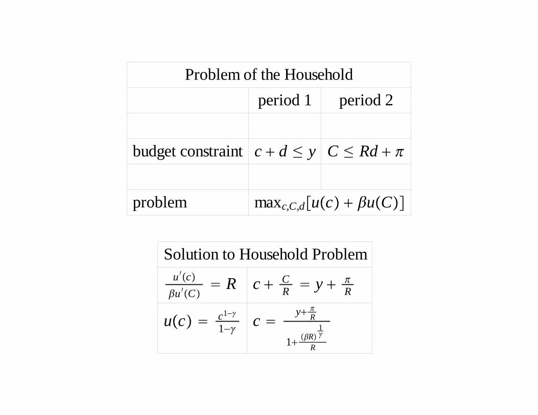
Solution to Household Problemu ′cu ′C

Rd c CRd ≤ y

Rd

uc c1−

1− c y

Rd

1Rd

1

Rd


Rd c CRd y

Rd

uc c1−

1− c y

Rd

1Rd

1

Rd

Problem of the Householdperiod 1 period 2

budget constraint c d ≤ y C ≤ Rdd

problem maxc,C,duc uC


Rd c CRd ≤ y

Rd

uc c1−

1− c y

Rd

1Rd

1

Rd


Rd c CRd y

Rd

uc c1−

1− c y

Rd

1Rd

1

Rd

Household budget constraint when gov’t buysprivate assets using tax receipts, T, and gov’tgets the same rate of return, Rd, as households:

c CRd y − T TRd

Rd y Rd

No change!(Ricardian‐WallaceIrrelevance)


Rd c CRd ≤ y

Rd

uc c1−

1− c y

Rd

1Rd

1

Rd


Rd c CRd y

Rd

uc c1−

1− c y

Rd

1Rd

1

Rd


budget constraint c d ≤ y C ≤ Rdd


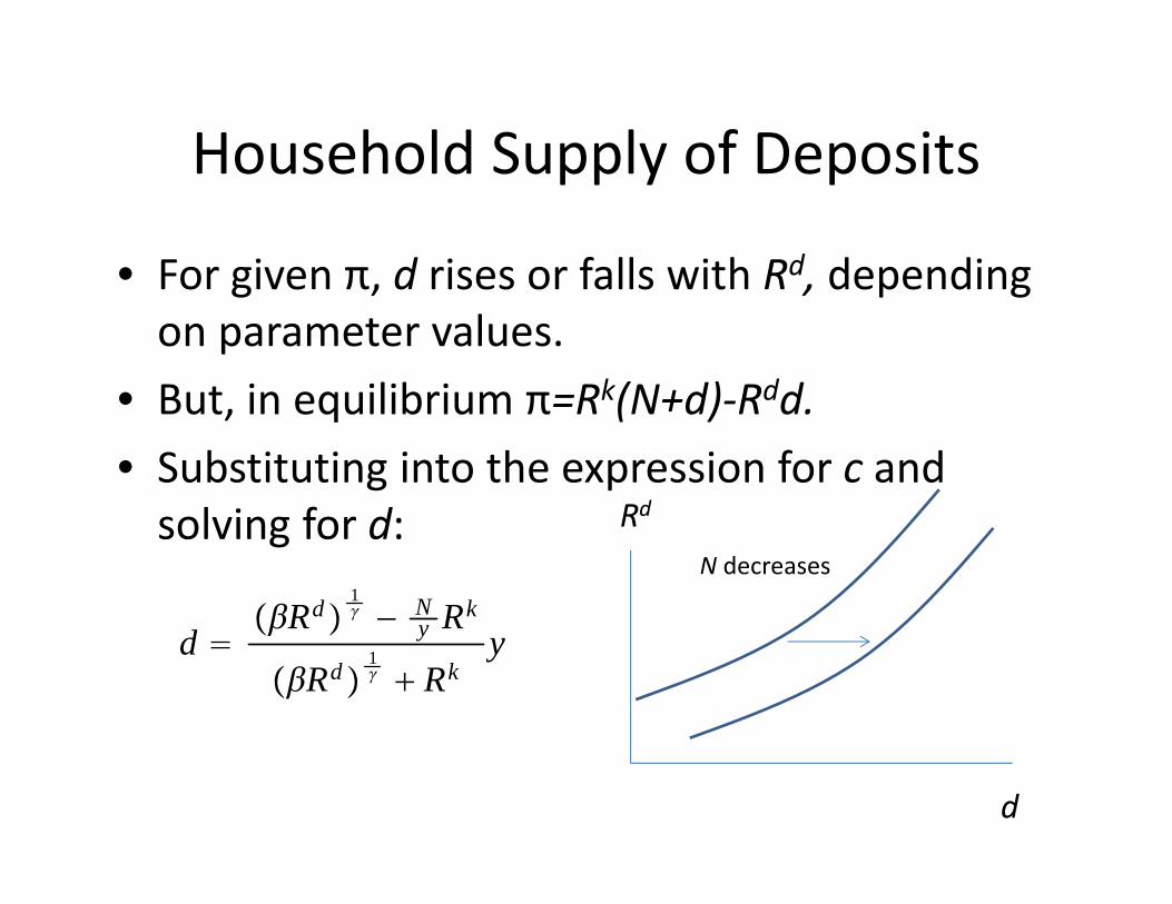
Household Supply of Deposits

• For given π, d rises or falls with Rd, depending on parameter values.

• But, in equilibrium π=Rk(N+d)‐Rdd. • Substituting into the expression for c and solving for d:

d Rd

1 − N

y Rk

Rd 1 Rk

y

d

Rd

Upward‐sloping deposit supply

Household Supply of Deposits

• For given π, d rises or falls with Rd, depending on parameter values.

• But, in equilibrium π=Rk(N+d)‐Rdd. • Substituting into the expression for c and solving for d:

d Rd

1 − N

y Rk

Rd 1 Rk

y

d

Rd

N decreases

Properties of Equilibrium Household Supply of Deposits

• Deposits increasing in Rd.

• Shifts right with decrease in N because of wealth effect operating via bank profits, π.– rise in deposit supply smaller than decrease in N.

∂d∂N −

0, 1

Rk

Rd 1 Rk

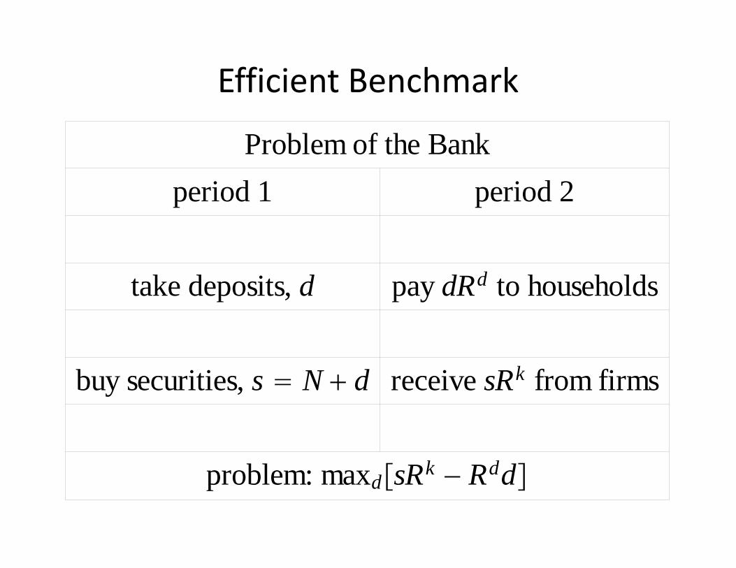
Efficient Benchmark

Problem of the Bankperiod 1 period 2

take deposits, d pay dRd to households

buy securities, s N d receive sRk from firms

problem: maxdsRk − Rdd

Bank demand for d

d

Rd

Demand for d by banks

Supply of d by households

Equilibrium d

Rk

Equilibrium in Absence of Frictions

• Properties:– Household faces true social rate of return on saving:

– Equilibrium is ‘first best’, i.e., solvesRk Rd

maxc,C,k, uc uCc k ≤ y N, C ≤ kRk

Interior Equilibrium: Rd,,d,c,C(i) c,d,C 0(ii) household problem is solved(iii) bank problem is solved(iv) goods and financial markets clear

Friction• bank combines deposits, d, with net worth, N, to purchase N+d securities from firms.

• bank has two options:– (‘no‐default’) wait until next period when arrives and pay off depositors, , for profit:

– (‘default’) take securities, refuse to pay depositors and wait until next period when securities pay off:

– Bank must announce what value of d it will choose at the beginning of a period.

N dRk

RddN dRk − Rdd

N d

N dRk

Incentive Constraint

• Recall, banks maximize profits

• Choose ‘no default’ iff

• Next: derive banking system’s demand for deposits in presence of financial frictions.

no default

N dRk − Rdd ≥

default

N dRk

Result for a no‐default equilibrium:• Consider an individual bank that contemplates deviating.

• It sets a d that implies default, , , or

• A deviating bank will in fact receive no deposits.• An optimizing bank would never default

– Can verify this is so if Rd > Rk, Rd = Rk, Rd < Rk.– Assume that in the case of indifference, they do not default.

what the household gets in the other banksRd

what the household gets in the defaulting bank

1 − Rkd Nd

RkN d − Rdd Rkd N

Problem of the bank in no‐default, interior equilibrium

• Maximize, by choice of d,

• subject to:

• or,

• Note that 0 < d < ∞ requires

RkN d − Rdd

RkN d − Rdd − RkN d ≥ 0,

1 − RkN − Rd − 1 − Rk d ≥ 0.

1 − Rkif not, then d Rd

if not, then d0≤ Rk.

Problem of the bank in no‐default, interior equilibrium, cnt’d

• For Rd = Rk

– a bank makes no profits on d so – absent default considerations ‐ it is indifferent over all values of 0≤d

– Taking into account default, a bank is indifferent over 0 ≤ d ≤ N(1‐θ)/θ

• For (1‐θ)Rk < Rd < Rk

– Bank wants d as large as possible, subject to incentive constraint.

– So, d = RkN(1‐θ)/(R‐(1‐θ)Rk)

Bank demand for dRd

d

Rk

(1‐θ)Rk

Bank demand for d

1− N

N1−1−1−Rk /Rd

Rk

Rd

Interior, no default equilibriumRd

d

Rk

Bank demand

Household supply

In this equilibrium, Rd = Rk and first‐best allocations occur. Banking system is highly effective in allocating resources efficiently.

Collapse in Bank Net Worth• Suppose that the economy is represented by a sequence of repeated versions of the above model.

• In the periods before the 2007‐2008 crisis, net worth was high and the equilibrium was like it is on the previous slide: efficient, with zero interest rate spreads.– In practice, spreads are always positive, but that reflects various banking costs that are left out of this model.

• With the crisis, N dropped a lot, shifting demand and supply to the left.– But, supply shifts more than demand, according to the model.

Effect of Substantial Drop in Bank Net WorthRd

d

Rk

Bank demand

Household supply

Equilibrium after N drops is inefficient because Rd < Rk.

Initial, efficient equilibrium

Government Intervention• Equity injection.

– Government raises T in period 1, provides proceeds to banks and demands RkT in return at start of period 2.

– Rebates earnings to households in 2.

• Has no impact on demand for deposits by banks (no impact on default incentive or profits).

• Reduces supply of deposits by households.

• Direct, tax‐financed government loans to firms work in the same way.

• An interest rate subsidy to banks will shift their demand for deposits to the right….it will also shift supply to the left.

Equity Injection and Drop in NRd

d

Rk

Bank demand

Household supply

Tax‐financed injection of equity into banks or direct loans to non‐financial firms shift householdsupply left.

Recap• Basic idea:

– Bankers can run away with a fraction of bank assets.

– If banker net worth is high relative to deposits, friction not a factor and banking system efficient.

– If banker net worth falls below a certain cutoff, then banker must restrict the deposits.

• Otherwise, depositors to lose confidence and take their business to another bank.

– Reduced supply of deposits:• makes deposit interest rates fall and so spreads rise.• Reduced intermediation means investment drops, output drops.

Next: another moral hazard model

• Previous model: bankers can run away with a fraction of bank assets.

• Now: bankers must make an unobserved and costly effort to identify good projects that make a high return for their depositors.– Bankers must have the right incentive to make that effort.

• Otherwise, model similar to previous one.

Model Has a Similar Diagnosis of the Financial Crisis as Moral Hazard I

• Both models articulate the idea:

• “…a fall in housing prices and other assets caused a fall in bank net worth and initiated a crisis. The banking system became dysfunctional as interest rate spreads increased and intermediation and economic activity was reduced. Various government policies can correct the situation’’

Two‐period Hidden Effort Model• Many identical households, each with a unit measure of

members:– Some members are ‘bankers’– Some members are ‘workers’– Perfect insurance inside households…everyone consumes same

amount.• Period 1

– Workers endowed with y goods, household makes deposits in a bank

– Bankers endowed with N goods, take deposits and make hidden efforts to identify a firm with a good investment project.

– Firm issues securities to finance capital used in production in period 2.

• Period 2– Household consumes earnings from deposits plus profits from

banker.– Goods consumed are produced by the firm.


Rd c CRd ≤ y

Rd

uc c1−

1− c y

Rd

1Rd

1

Rd


budget constraint c d ≤ y C ≤ Rd


Household problem in hidden banker effort model is same as in moral hazard I

slight changein notation.


Rd c CRd ≤ y

Rd

uc c1−

1− c y

Rd

1Rd

1

Rd


budget constraint c d ≤ y C ≤ Rd



R c CR y

R

uc c1−

1− c y

R

1 R1

R

Banker Problem• Bankers combine their net worth, N, and deposits, d, to acquire the securities of a single firm.– Bankers not diversified.

• Firms:– Good firms: investment project with return, – Bad firms: an investment project with return,

• Banker makes a costly, unobserved effort, e, to locate a good firm, and finds one with probability, p(e).– p(e) increasing in e.

Rg

Rb

Banker Problem, cnt’d• Mean and variance on banker’s asset:

• Note: – Mean increases in e– For p(e)>1/2,

• Variance of the portfolio decreases with increase in e

mean: peRg 1 − peRb

variance: pe1 − peRg − Rb 2

derivative of variance w.r.t. e:

1 − 2peRg − Rb 2p′e,

Funding for Bankers

• Representative household deposits money into a representative mutual fund.– Household receives a certain return, R.

• Representative mutual fund acquires deposit, d, in each of a diversified set of banks.– Mutual fund receives from p(e) banks with a good investment.

– Mutual fund receives from 1‐p(e) banks with a bad investment.

dRgd

dRbd

Risky Bankers Funded By Mutual Funds

Diversified,competitivemutual funds

Household

banker

banker

banker

banker

Household

Household

Arrangement Between Banks and Mutual Funds

• Contract traded in competitive market:

Deposit amount effort

d,e,Rgd,Rb

d

Interest rate in good state

Interest rate in bad state

Two Versions of Model• No financial frictions: mutual fund observes banker effort.– This is the benchmark version.

• Financial frictions: mutual fund does not observe banker effort.– This is the interesting version. – Use it to think about crisis in 2008‐2009, and unconventional monetary policy.

Equilibrium Contract When Effort is Observable

• Competition and free entry among mutual funds:

• Zero profit condition represents a menu of contracts available to banks.

money owed to households by mutual fundsRd

fraction of banks with good investmentspe Rg

dd

fraction of banks with bad investments

1 − pe Rbdd

Contract Selected by Banks in Observable Effort Equilibrium

Marginal value assigned by household to bank profits

maxe,d,Rg

d,Rbd

expected bank profits

peRgN d − Rgdd 1 − peRbN d − Rb

dd

−

utility cost of effort suffered by banker12 e2

subject to:

zero profit condition of mutual funds

Rd peRgdd 1 − peRb

dd,

cash flow constraint on banks

RbN d ≥ Rbdd

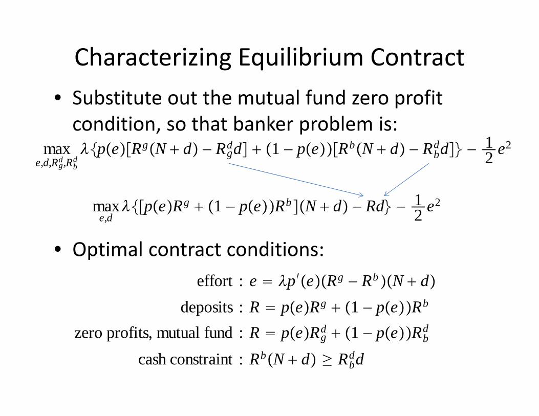
Characterizing Equilibrium Contract • Substitute out the mutual fund zero profit condition, so that banker problem is:

• Optimal contract conditions:

maxe,d,Rg

d,RbdpeRgN d − Rg

dd 1 − peRbN d − Rbdd − 1

2 e2

maxe,d

peRg 1 − peRb N d − Rd − 12 e2

effort : e p′eRg − RbN ddeposits : R peRg 1 − peRb

zero profits, mutual fund : R peRgd 1 − peRb

d

cash constraint : RbN d ≥ Rbdd

Properties of Contract• Banker treats d and N symmetrically

• Other equations:

• Algorithm:– Fix R, get c, C, d from household problem– Compute e from effort equation (use )– Adjust R until deposits equation is satisfied.

• Returns on deposits not uniquely pinned down. Cash constraint not binding.– N large enough relative to d, can choose

effort : e p′eRg − Rb N ddeposits : R peRg 1 − peRb


d


Rgd Rb

d R

pe a be, b 0.

Observable Effort Equilibrium

Observable Effort Equilibrium: c, C, e, d, R, , Rgd, Rb

d such that(i) the household maximization problem is solved(ii) mutual funds earn zero profits(iii) the banker problem with e observable, is solved(iv) markets clear(v) c,C,d,e 0

Unobservable Effort• Suppose that the banker has obtained a contract, , from the mutual fund.

• The mutual fund can observe so that the banker no longer has any choice about these.

• The mutual fund does not observe e, and so the bank can still choose e freely after the contract has been selected.

• The banker solves

d,e,Rgd,Rb

d

d,Rgd,Rb

d

maxepeRgN d − Rg


2 e2

Incentive Constraint• Banker choice of e after the deposit contract has been selected:

• First order condition:

– Note: if then the banker exerts less effort than in the observable effort equilibrium.

– Reason is that the banker does not receive the full return on its effort if

maxepeRgN d − Rg


2 e2

e p′eRg − Rb N d − Rgd − Rb

d d

Rgd Rb

d

Rgd Rb

d

Unobservable Effort Equilibrium• Mutual funds are only willing to consider contracts, , that satisfy the following restrictions:

• There is no point for the mutual fund to consider a contract in which e does not satisfy the last condition, since bankers will set eaccording to the last condition in any case.


d


incentive compatibility: e p′eRg − Rb N d − Rgd − Rb

dd

d,e,Rgd,Rb

d

Contract Selected by Banks in Unobservable Effort Equilibrium

• Solve

• Subject to

maxe,d,Rg

d,RbdpeRgN d − Rg

dd 1 − peRbN d − Rbdd

− 12 e2


d


incentive compatibility: e p′eRg − RbN d − Rgd − Rb

dd

Two Unobservable Effort Equilibria• Case 1: Banker net worth, N, is high enough

– Recall the two conditions on deposit returns:

– Suppose that N is large enough so that given d from the observable effort equilibrium, cash constraint is satisfied with

– Then, observable effort equilibrium is also an unobservable effort equilibrium.

• With N large enough, unobservable effort equilibrium is efficient.


d


Rgd Rb

d R

Risk Premium• R is the risk free rate in the model (i.e., the sure return received by the household).

• Let denote the ‘bank interest rate on deposits’. – This is what the bank pays in the event that its portfolio is ‘good’.

• Risk premium:

• Result: when N is high enough, equilibrium level of intermediation is efficient and risk premium is zero.

Rgd

Rgd − R

Case 2: Banker net worth, N, is low• Recall the two conditions on deposit returns:

– Suppose that N is small, so that given d from the observable effort equilibrium, cash constraint is not satisfied with

– Then, observable effort equilibrium is not an unobservable effort equilibrium.

• With N small enough, unobservable effort equilibrium is not efficient.


d


Rgd Rb

d R

Unobserved Effort Equilibrium, low N Case• The two conditions on deposit returns:

• Suppose, with efficient d and e, cash constraint is not satisfied for . Then

– Set – Risk premium positive – Incentive constraint implies inefficiently low e.– Low e implies low R, which implies low d.

• Banking system ‘dysfunctional’.– Mean of bank return goes down, and variance up.


d


Rbd R

Rbd R, Rg

d R (still have R peRg 1 − peRb)

Scenario Rationalized by Model• Before 2007, when N was high, the banking system

supported the efficient allocations and the interest spread was zero.

• The fall in bank net worth after 2007, caused a jump in the risk premium, and a slowdown in intermediation and investment.

• Banking system became dysfunctional because banks did not have enough net worth to cover possible losses.– This meant depositors had to take losses in case of a bad

investment outcome in banks. – Depositors require a high return in good states as

compensation: risk premium.– Bankers lose incentive to exert high effort. More bad projects

are funded, reducing the overall return on saving.– Saving falls below its efficient level.

How to Fix the Problem• One solution: tax the workers and transfer the proceeds to bankers

so they have more net worth.– In the model, this is a good idea because income distribution issues

have been set aside.– In practice, income distribution problems could be a serious concern

and this policy may therefore not be feasible

• Subsidize the interest rate costs of banks. – This increases the chance that bank net worth is sufficient to cover

losses, reduces the risk premium and gives bankers an incentive to increase effort.

– Increased effort increases the return on banker portfolios and reduces their variance.

• Equity injections and loans to banks have zero impact in the model, when it is in a bad equilibrium. – Ricardian irrelevance not overturned.– the sources of moral hazard matter for whether a particular asset

purchase programs is effective!

Conclusion• Have described two models of moral hazard, that can rationalize the view:– Bank net worth fell, causing interest rate spreads to jump and intermediation to slow down. The banking system is dysfunctional.

• Net worth transfers and interest rate subsidies can revive a dysfunctional banking system in both models.

• However, the models differ in terms of the detailed economic story, as well as in terms of their implications for asset purchases.

two financial friction models - northwestern...

Documents