two improved gauss-seidel projection methods for landau ... · two improved gauss-seidel projection...

Two improved Gauss-Seidel projection methods forLandau-Lifshitz-Gilbert equation

Panchi Lia, Changjian Xiea, Rui Dua,b,∗, Jingrun Chena,b,∗, Xiao-Ping Wangc,∗

aSchool of Mathematical Sciences, Soochow University, Suzhou, 215006, China.bMathematical Center for Interdisciplinary Research, Soochow University, Suzhou, 215006, China.cDepartment of Mathematics, The Hong Kong University of Science and Technology, Clear Water Bay,Kowloon, Hong Kong, China

A B S T R A C T

Micromagnetic simulation is an important tool to study various dynamic behaviors ofmagnetic order in ferromagnetic materials. The underlying model is the Landau-Lifshitz-Gilbert equation, where the magnetization dynamics is driven by the gyromagnetic torqueterm and the Gilbert damping term. Numerically, considerable progress has been made inthe past decades. One of the most popular methods is the Gauss-Seidel projection methoddeveloped by Xiao-Ping Wang, Carlos Garcıa-Cervera, and Weinan E in 2001. It first solvesa set of heat equations with constant coefficients and updates the gyromagnetic term in theGauss-Seidel manner, and then solves another set of heat equations with constant coefficientsfor the damping term. Afterwards, a projection step is applied to preserve the length con-straint in the pointwise sense. This method has been verified to be unconditionally stablenumerically and successfully applied to study magnetization dynamics under various controls.

In this paper, we present two improved Gauss-Seidel projection methods with uncondi-tional stability. The first method updates the gyromagnetic term and the damping termsimultaneously and follows by a projection step. The second method introduces two sets ofapproximate solutions, where we update the gyromagnetic term and the damping term simul-taneously for one set of approximate solutions and apply the projection step to the other setof approximate solutions in an alternating manner. Compared to the original Gauss-Seidelprojection method which has to solve heat equations 7 times at each time step, the improvedmethods solve heat equations 5 times and 3 times, respectively. First-order accuracy in timeand second-order accuracy in space are verified by examples in both 1D and 3D. In addi-tion, unconditional stability with respect to both the grid size and the damping parameter isconfirmed numerically. Application of both methods to a realistic material is also presentedwith hysteresis loops and magnetization profiles. Compared with the original method, therecorded running times suggest that savings of both methods are about 2/7 and 4/7 for thesame accuracy requirement, respectively.

Keywords: Landau-Lifshitz-Gilbert equation, Gauss-Seidel projection method, unconditionalstability, micromagnetic simulation2000 MSC: 35Q99, 65Z05, 65M06

1. Introduction

In ferromagnetic materials, the intrinsic magnetic order, known as magnetization M =

(M1,M2,M3)T , is modeled by the following Landau-Lifshitz-Gilbert (LLG) equation [1, 2, 3]

∂M

∂t= −γM×H− γα

MsM× (M×H) (1)

∗Corresponding authorse-mail: [email protected] (Panchi Li), [email protected] (Changjian Xie),

[email protected] (Rui Du), [email protected] (Jingrun Chen), [email protected] (Xiao-Ping Wang)

1

arX

iv:1

907.

1185

3v1

[m

ath.

NA

] 2

7 Ju

l 201

9

with γ the gyromagnetic ratio and |M| = Ms the saturation magnetization. On the right-

hand side of (1), the first term is the gyromagnetic term and the second term is the Gilbert

damping term with α the dimensionless damping coefficient [2]. Note that the gyromagnetic

term is a conservative term, whereas the damping term is a dissipative term. The local field

H = − δFδM is computed from the Landau-Lifshitz energy functional

F [M] =1

2

∫Ω

A

M2s

|∇M|2 + Φ

(M

Ms

)− 2µ0He ·M

dx+

µ0

2

∫R3

|∇U |2dx, (2)

where A is the exchange constant, AM2

s|∇M| is the exchange interaction energy; Φ

(MMs

)is the anisotropy energy, and for simplicity the material is assumed to be uniaxial with

Φ(

MMs

)= Ku

M2s

(M22 + M2

3 ) with Ku the anisotropy constant; −2µ0He ·M is the Zeeman

energy due to the external field with µ0 the permeability of vacuum. Ω is the volume occupied

by the material. The last term in (2) is the energy resulting from the field induced by the

magnetization distribution inside the material. This stray field Hs = −∇U where U(x)

satisfies

U(x) =

∫Ω

∇N(x− y) ·M(y)dy, (3)

where N(x− y) = − 14π

1|x−y| is the Newtonian potential.

For convenience, we rescale the original LLG equation (1) by changes of variables t →

(µ0γMs)−1t and x→ Lx with L the diameter of Ω. Define m = M/Ms and h = MsH. The

dimensionless LLG equation reads as

∂m

∂t= −m× h− αm× (m× h), (4)

where

h = −Q(m2e2 +m3e3) + ε∆m + he + hs (5)

with dimensionless parameters Q = Ku/(µ0M2s ) and ε = A/(µ0M

2sL

2). Here e2 = (0, 1, 0),

e3 = (0, 0, 1). Neumann boundary condition is used

∂m

∂ν |∂Ω= 0, (6)

where ν is the outward unit normal vector on ∂Ω.

The LLG equation is a weakly nonlinear equation. In the absence of Gilbert damping,

α = 0, equation (4) is a degenerate equation of parabolic type and is related to the sympletic

flow of harmonic maps [4]. In the large damping limit, α → ∞, equation (4) is related to

the heat flow for harmonic maps [5]. It is easy to check that |m| = 1 in the pointwise sense

in the evolution. All these properties possesses interesting challenges for designing numerical

methods to solve the LLG equation. Meanwhile, micromagnetic simulation is an important

tool to study magnetization dynamics of magnetic materials [3, 6]. Over the past decades,

there has been increasing progress on numerical methods for the LLG equation; see [7, 8, 9]

2

for reviews and references therein. Finite difference method and finite element method have

been used for the spatial discretization.

For the temporal discretization, there are explicit schemes such as Runge-Kutta methods

[10, 11]. Their stepsizes are subject to strong stability constraint. Another issue is that the

length of magnetization cannot be preserved and thus a projection step is needed. Implicit

schemes [12, 13, 14] are unconditionally stable and usually can preserve the length of magne-

tization automatically. The difficulty of implicit schemes is how to solve a nonlinear system

of equations at each step. Therefore, semi-implicit methods [15, 16, 17, 18, 19] provide a com-

promise between stability and the difficult for solving the equation at each step. A projection

step is also needed to preserve the length of magnetization.

Among the semi-implicit schemes, the most popular one is the Gauss-Seidel projection

method (GSPM) proposed by Wang, Garcıa-Cervera, and E [15, 18]. GSPM first solves a

set of heat equations with constant coefficients and updates the gyromagnetic term in the

Gauss-Seidel manner, and then solves another set of heat equations with constant coefficients

for the damping term. Afterwards, a projection step is applied to preserve the length of mag-

netization. GSPM is first-order accurate in time and has been verified to be unconditionally

stable numerically.

In this paper, we present two improved Gauss-Seidel projection methods with uncondi-

tional stability. The first method updates the gyromagnetic term and the damping term

simultaneously and follows by a projection step. The second method introduces two sets of

approximate solutions, where we update the gyromagnetic term and the damping term simul-

taneously for one set of approximate solutions and apply the projection step to the other set

of approximate solutions in an alternating manner. Compared to the original Gauss-Seidel

projection method, which solves heat equations 7 times at each time step, the improved

methods solve heat equations 5 times and 3 times, respectively. First-order accuracy in time

and second-order accuracy in space are verified by examples in both 1D and 3D. In addi-

tion, unconditional stability with respect to both the grid size and the damping parameter is

confirmed numerically. Application of both methods to a realistic material is also presented

with hysteresis loops and magnetization profiles. Compared with the original method, the

recorded running times suggest that savings of both methods are about 2/7 and 4/7 for the

same accuracy requirement, respectively.

The rest of the paper is organized as follows. For completeness and comparison, we first

introduce GSPM in Section 2. Two improved GSPMs are presented in Section 3. Detailed

numerical tests are given in Section 4, including accuracy check and efficiency check in both

1D and 3D, unconditional stability with respect to both the grid size and the damping

parameter, hysteresis loops, and magnetization profiles. Conclusions are drawn in Section 5.

3

2. Gauss-Seidel projection method for Landau-Lifshitz-Gilbert equation

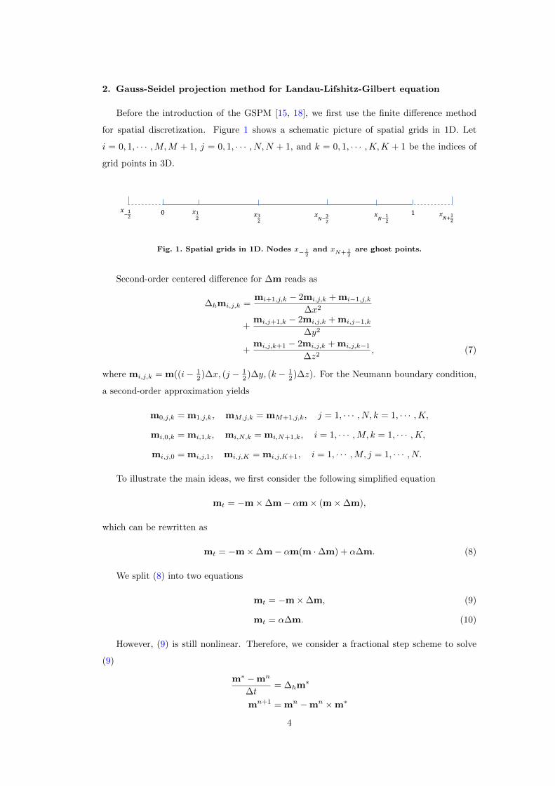
Before the introduction of the GSPM [15, 18], we first use the finite difference method

for spatial discretization. Figure 1 shows a schematic picture of spatial grids in 1D. Let

i = 0, 1, · · · ,M,M + 1, j = 0, 1, · · · , N,N + 1, and k = 0, 1, · · · ,K,K + 1 be the indices of

grid points in 3D.

0 1𝑥−12

𝑥12

𝑥𝑁−

12

𝑥𝑁+

12

𝑥32

𝑥𝑁−

32

Fig. 1. Spatial grids in 1D. Nodes x− 12

and xN+ 12

are ghost points.

Second-order centered difference for ∆m reads as

∆hmi,j,k =mi+1,j,k − 2mi,j,k + mi−1,j,k

∆x2

+mi,j+1,k − 2mi,j,k + mi,j−1,k

∆y2

+mi,j,k+1 − 2mi,j,k + mi,j,k−1

∆z2, (7)

where mi,j,k = m((i− 12 )∆x, (j − 1

2 )∆y, (k − 12 )∆z). For the Neumann boundary condition,

a second-order approximation yields

m0,j,k = m1,j,k, mM,j,k = mM+1,j,k, j = 1, · · · , N, k = 1, · · · ,K,

mi,0,k = mi,1,k, mi,N,k = mi,N+1,k, i = 1, · · · ,M, k = 1, · · · ,K,

mi,j,0 = mi,j,1, mi,j,K = mi,j,K+1, i = 1, · · · ,M, j = 1, · · · , N.

To illustrate the main ideas, we first consider the following simplified equation

mt = −m×∆m− αm× (m×∆m),

which can be rewritten as

mt = −m×∆m− αm(m ·∆m) + α∆m. (8)

We split (8) into two equations

mt = −m×∆m, (9)

mt = α∆m. (10)

However, (9) is still nonlinear. Therefore, we consider a fractional step scheme to solve

(9)

m∗ −mn

∆t= ∆hm

∗

mn+1 = mn −mn ×m∗

4

or

mn+1 = mn −mn × (I −∆t∆h)−1mn,

where I is the identity matrix. This scheme is subject to strong stability constraint, and thus

the implicit Gauss-Seidel scheme is introduced to overcome this issue. Let

gni = (I −∆t∆h)−1mni , i = 1, 2, 3. (11)

We then have mn+11

mn+12

mn+13

=

mn1 + (gn2m

n3 − gn3mn

2 )mn

2 + (gn3mn+11 − gn+1

1 mn3 )

mn3 + (gn+1

1 mn+12 − gn+1

2 mn+11 )

. (12)

This scheme solve (9) with unconditional stability. (10) is linear heat equation which can be

solved easily. However, the splitting scheme (9) - (10) cannot preserve |m| = 1, and thus a

projection step needs to be added.

For the full LLG equation (4), the GSPM works as follows. Define

h = ε∆m + f , (13)

where f = −Q(m2e2 +m3e3) + he + hs.

The original GSPM [15] solves the equation (4) in three steps:

• Implicit Gauss-Seidel

gni = (I −∆tε∆h)−1(mni + ∆tfni ), i = 2, 3,

g∗i = (I −∆tε∆h)−1(m∗i + ∆tfni ), i = 1, 2, (14)m∗1m∗2m∗3

=

mn1 + (gn2m

n3 − gn3mn

2 )mn

2 + (gn3m∗1 − g∗1mn

3 )mn

3 + (g∗1m∗2 − g∗2m∗1)

. (15)

• Heat flow without constraints

f∗ = −Q(m∗2e2 +m∗3e3) + he + hns , (16)

m∗∗1m∗∗2m∗∗3

=

m∗1 + α∆t(ε∆hm∗∗1 + f∗1 )

m∗2 + α∆t(ε∆hm∗∗2 + f∗2 )

m∗3 + α∆t(ε∆hm∗∗3 + f∗3 )

. (17)

• Projection onto S2 mn+11

mn+12

mn+13

=1

|m∗∗|

m∗∗1m∗∗2m∗∗3

. (18)

Here the numerical stability of the original GSPM [15] was founded to be independent of

gridsizes but depend on the damping parameter α. This issue was solved in [18] by replacing

(14) and (16) with

g∗i = (I −∆tε∆h)−1(m∗i + ∆tf∗i ), i = 1, 2,

5

and

f∗ = −Q(m∗2e2 +m∗3e3) + he + h∗s,

respectively. Update of the stray field is done using fast Fourier transform [15]. It is easy

to see that the GSPM solves 7 linear systems of equations with constant coefficients and

updates the stray field using FFT 6 times at each step.

3. Two improved Gauss-Seidel projection methods for Landau-Lifshitz-Gilbertequation

Based on the description of the original GSPM in Section 2, we introduce two improved

GSPMs for LLG equation. The first improvement updates both the gyromagnetic term and

the damping term simultaneously, termed as Scheme A. The second improvement introduces

two sets of approximate solution with one set for implicit Gauss-Seidel step and the other set

for projection in an alternating manner, termed as Scheme B. Details are given in below.

3.1. Scheme A

The main improvement of Scheme A over the original GSPM is the combination of (13)

- (17), or (9) - (10).

• Implicit-Gauss-Seidel

gni = (I −∆tε∆h)−1(mni + ∆tfni ), i = 1, 2, 3,

g∗i = (I −∆tε∆h)−1(m∗i + ∆tf∗i ), i = 1, 2, (19)m∗1m∗2m∗3

=

mn1 − (mn

2 gn3 −mn

3 gn2 )− α(mn

1 gn1 +mn

2 gn2 +mn

3 gn3 )mn

1 + αgn1mn

2 − (mn3 g∗1 −m∗1gn3 )− α(m∗1g

∗1 +mn

2 gn2 +mn

3 gn3 )mn

2 + αgn2mn

3 − (m∗1g∗2 −m∗2g∗1)− α(m∗1g

∗1 +m∗2g

∗2 +mn

3 gn3 )mn

3 + αgn3

. (20)


mn+12

mn+13

=1

|m∗|

m∗1m∗2m∗3

. (21)

It is easy to see that Scheme A solves 5 linear systems of equations with constant coefficients

and uses FFT 5 times at each step.

3.2. Scheme B

The main improvement of Scheme B over Scheme A is the introduction of two sets of

approximate solutions, one for (19) - (20) and the other for (21) and the update of these two

sets of solutions in an alternating manner.

Given the initialized g0

g0i = (I −∆tε∆h)−1(m0

i + ∆tf0i ), i = 1, 2, 3, (22)

Scheme B works as follows

6

• Implicit Gauss-Seidel

gn+1i = (I −∆tε∆h)−1(m∗i + ∆tf∗i ), i = 1, 2, 3 (23)

m∗1 = mn1 − (mn

2 gn3 −mn

3 gn2 )− α(mn

1 gn1 +mn

2 gn2 +mn

3 gn3 )mn

1 +

α((mn1 )2 + (mn

2 )2 + (mn3 )2)gn1

m∗2 = mn2 − (mn

3 gn+11 −m∗1gn3 )− α(m∗1g

n+11 +mn

2 gn2 +mn

3 gn3 )mn

2 +

α((m∗1)2 + (mn2 )2 + (mn

3 )2)gn2

m∗3 = mn3 − (m∗1g

n+12 −m∗2gn+1

1 )− α(m∗1gn+11 +m∗2g

n+12 +mn

3 gn3 )mn

3 +

α((m∗1)2 + (m∗2)2 + (mn3 )2)gn3 (24)


mn+12

mn+13

=1

|m∗|

m∗1m∗2m∗3

. (25)

Here one set of approximate solution m∗ is updated in the implicit Gauss-Seidel step and

the other set of approximate solution mn+1 is updated in the projection step. Note that

(23) is defined only for m∗ which can be used in two successive temporal steps, and thus

only 3 linear systems of equations with constant coefficients are solved at each step and 3

FFT executions are used for the stray field. The length of magnetization can be preserved

in the time evolution.

The computational cost of GSPM and its improvements comes from solving the linear

systems of equations with constant coefficients. To summarize, we list the number of linear

systems of equations to be solved and the number of FFT executions to be used at each step

for the original GSPM [18], Scheme A, and Scheme B in Table 1. The savings represent the

ratio between costs of two improved schemes over that of the original GSPM.

GSPM Scheme Number of linear systems Saving Execution of FFT SavingOriginal 7 0 4 0

Scheme A 5 2/7 3 1/4Scheme B 3 4/7 3 1/4

Table 1. The number of linear systems of equations to be solved and the number of FFTexecutions to be used at each step for the original GSPM [18], Scheme A, and Scheme B. Thesavings represent the ratio between costs of two improved schemes over that of the originalGSPM.

4. Numerical Experiments

In this section, we compare the original GSPM [15, 18], Scheme A, and Scheme B via a

series of examples in both 1D and 3D, including accuracy check and efficiency check, uncon-

ditional stability with respect to both the grid size and the damping parameter, hysteresis

7

loops, and magnetization profiles. For convenience, we define

ratio− i =Time(GSPM)− Time(Scheme i)

Time(GSPM),

for i = A and B, which quantifies the improved efficiency of Scheme A and Scheme B over

the original GSPM [15, 18].

4.1. Accuracy Test

Example 4.1 (1D case). In 1D, we choose the exact solution over the unit interval Ω =

[0, 1]

me = (cos(x) sin(t), sin(x) sin(t), cos(t)),

which satisfies

mt = −m×mxx − αm× (m×mxx) + f

with x = x2(1 − x)2, and f = met + me ×mexx + αme × (me ×mexx). Parameters are

α = 0.00001 and T = 5.0e− 2.

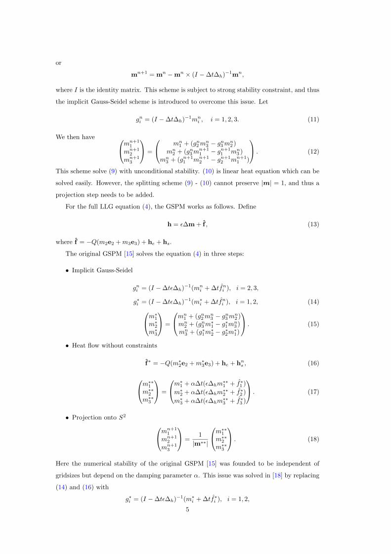
We first show the error ‖me −mh‖∞ with mh being the numerical solution with respect

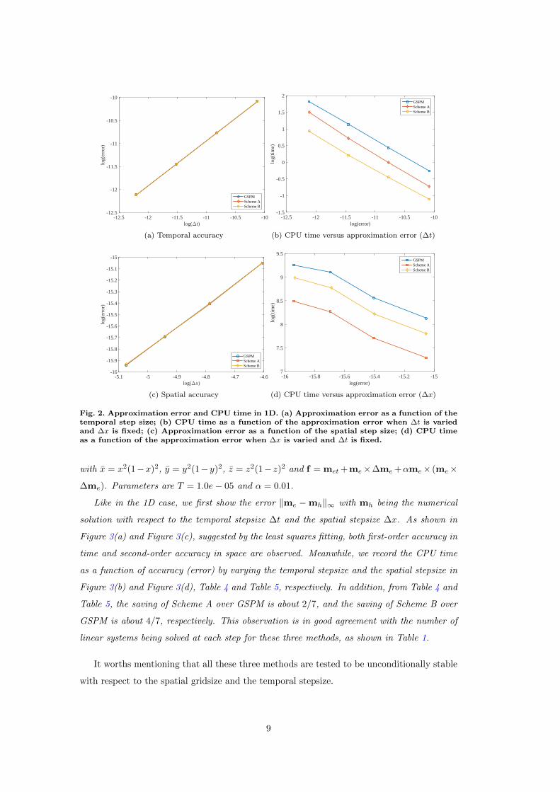
to the temporal stepsize ∆t and the spatial stepsize ∆x. As shown in Figure 2(a) and Fig-

ure 2(c), suggested by the least squares fitting, both first-order accuracy in time and second-

order accuracy in space are observed. Meanwhile, we record the CPU time as a function

of accuracy (error) by varying the temporal stepsize and the spatial stepsize in Figure 2(b)

and Figure 2(d), Table 2 and Table 3, respectively. In addition, from Table 2 and Table 3,

the saving of Scheme A over GSPM is about 2/7, which equals 1 − 5/7, and the saving of

Scheme B over GSPM is about 4/7, respectively. This observation is in good agreement with

the number of linear systems being solved at each step for these three methods, as shown in

Table 1.

XXXXXXXXXXCPU time∆t

T/1250 T/2500 T/5000 T/10000 Reference

GSPM 7.7882e-01 1.5445e+00 3.1041e+00 6.2196e+00 -Scheme A 4.8340e-01 9.9000e-01 2.0527e+00 4.4917e+00 -Scheme B 3.3010e-01 6.3969e-01 1.2281e+00 2.5510e+00 -ratio-A 0.38 0.36 0.34 0.28 0.29(2/7)ratio-B 0.58 0.59 0.60 0.59 0.57(4/7)

Table 2. Recorded CPU time in 1D with respect to the approximation error when only ∆t isvaried and ∆x = 1/100.

Example 4.2 (3D case). In 3D, we choose the exact solution over Ω = [0, 2]×[0, 1]×[0, 0.2]

me = (cos(xyz) sin(t), sin(xyz) sin(t), cos(t)),

which satisfies

mt = −m×∆m− αm× (m×∆m) + f

8

log(∆t)-12.5 -12 -11.5 -11 -10.5 -10

log(

erro

r)

-12.5

-12

-11.5

-11

-10.5

-10

GSPMScheme AScheme B

(a) Temporal accuracy

log(error)-12.5 -12 -11.5 -11 -10.5 -10

log(

time)

-1.5

-1

-0.5

0

0.5

1

1.5

2GSPMScheme AScheme B

(b) CPU time versus approximation error (∆t)

log(∆x)-5.1 -5 -4.9 -4.8 -4.7 -4.6

log(

erro

r)

-16

-15.9

-15.8

-15.7

-15.6

-15.5

-15.4

-15.3

-15.2

-15.1

-15


(c) Spatial accuracy

log(error)-16 -15.8 -15.6 -15.4 -15.2 -15

log(

time)

7

7.5

8

8.5

9

9.5GSPMScheme AScheme B

(d) CPU time versus approximation error (∆x)

Fig. 2. Approximation error and CPU time in 1D. (a) Approximation error as a function of thetemporal step size; (b) CPU time as a function of the approximation error when ∆t is variedand ∆x is fixed; (c) Approximation error as a function of the spatial step size; (d) CPU timeas a function of the approximation error when ∆x is varied and ∆t is fixed.

with x = x2(1−x)2, y = y2(1−y)2, z = z2(1− z)2 and f = met+me×∆me+αme× (me×

∆me). Parameters are T = 1.0e− 05 and α = 0.01.

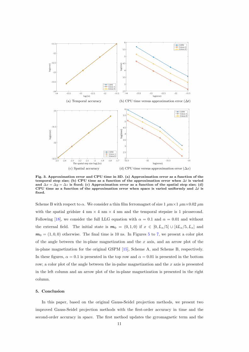
Like in the 1D case, we first show the error ‖me −mh‖∞ with mh being the numerical

solution with respect to the temporal stepsize ∆t and the spatial stepsize ∆x. As shown in

Figure 3(a) and Figure 3(c), suggested by the least squares fitting, both first-order accuracy in

time and second-order accuracy in space are observed. Meanwhile, we record the CPU time

as a function of accuracy (error) by varying the temporal stepsize and the spatial stepsize in

Figure 3(b) and Figure 3(d), Table 4 and Table 5, respectively. In addition, from Table 4 and

Table 5, the saving of Scheme A over GSPM is about 2/7, and the saving of Scheme B over

GSPM is about 4/7, respectively. This observation is in good agreement with the number of

linear systems being solved at each step for these three methods, as shown in Table 1.

It worths mentioning that all these three methods are tested to be unconditionally stable

with respect to the spatial gridsize and the temporal stepsize.

9

XXXXXXXXXXCPU time∆x

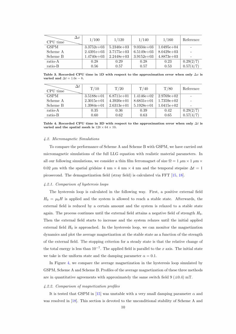
1/100 1/120 1/140 1/160 Reference

GSPM 3.3752e+03 5.2340e+03 9.0334e+03 1.0495e+04 -Scheme A 2.4391e+03 3.7175e+03 6.5149e+03 8.0429e+03 -Scheme B 1.4740e+03 2.2448e+03 3.9152e+03 4.8873e+03 -ratio-A 0.28 0.29 0.28 0.23 0.29(2/7)ratio-B 0.56 0.57 0.57 0.53 0.57(4/7)

Table 3. Recorded CPU time in 1D with respect to the approximation error when only ∆x isvaried and ∆t = 1.0e− 8.

XXXXXXXXXXCPU time∆t

T/10 T/20 T/40 T/80 Reference


Table 4. Recorded CPU time in 3D with respect to the approximation error when only ∆t isvaried and the spatial mesh is 128 × 64 × 10.

4.2. Micromagnetic Simulations

To compare the performance of Scheme A and Scheme B with GSPM, we have carried out

micromagnetic simulations of the full LLG equation with realistic material parameters. In

all our following simulations, we consider a thin film ferromagnet of size Ω = 1 µm× 1 µm×

0.02 µm with the spatial gridsize 4 nm × 4 nm × 4 nm and the temporal stepsize ∆t = 1

picosecond. The demagnetization field (stray field) is calculated via FFT [15, 18].

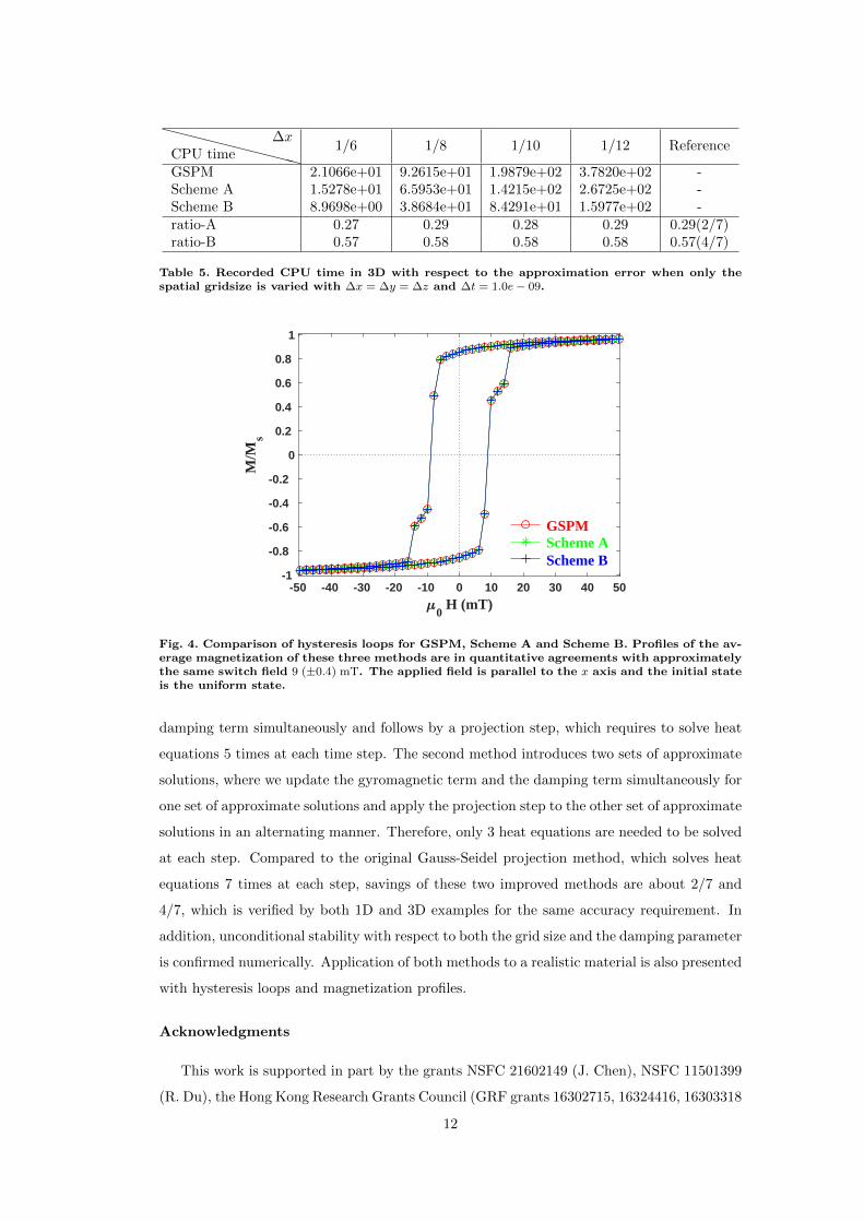
4.2.1. Comparison of hysteresis loops

The hysteresis loop is calculated in the following way. First, a positive external field

H0 = µ0H is applied and the system is allowed to reach a stable state. Afterwards, the

external field is reduced by a certain amount and the system is relaxed to a stable state

again. The process continues until the external field attains a negative field of strength H0.

Then the external field starts to increase and the system relaxes until the initial applied

external field H0 is approached. In the hysteresis loop, we can monitor the magnetization

dynamics and plot the average magnetization at the stable state as a function of the strength

of the external field. The stopping criterion for a steady state is that the relative change of

the total energy is less than 10−7. The applied field is parallel to the x axis. The initial state

we take is the uniform state and the damping parameter α = 0.1.

In Figure 4, we compare the average magnetization in the hysteresis loop simulated by

GSPM, Scheme A and Scheme B. Profiles of the average magnetization of these three methods

are in quantitative agreements with approximately the same switch field 9 (±0.4) mT.

4.2.2. Comparison of magnetization profiles

It is tested that GSPM in [15] was unstable with a very small damping parameter α and

was resolved in [18]. This section is devoted to the unconditional stability of Scheme A and

10

log(∆t)-14 -13.5 -13 -12.5 -12 -11.5

log(

erro

r)

-14

-13.5

-13

-12.5

-12

-11.5


(a) Temporal accuracy

log(error)-14 -13.5 -13 -12.5 -12 -11.5

log(

time)

2.5

3

3.5

4

4.5

5

5.5


(b) CPU time versus approximation error (∆t)

The spatial step size log(∆x)-2.5 -2.4 -2.3 -2.2 -2.1 -2 -1.9 -1.8 -1.7

log(

erro

r)

-32.5

-32

-31.5

-31


(c) Spatial accuracy

log(error)-32.5 -32 -31.5 -31

log(

time)

2

2.5

3

3.5

4

4.5

5

5.5


(d) CPU time versus approximation error (∆x)

Fig. 3. Approximation error and CPU time in 3D. (a) Approximation error as a function of thetemporal step size; (b) CPU time as a function of the approximation error when ∆t is variedand ∆x = ∆y = ∆z is fixed; (c) Approximation error as a function of the spatial step size; (d)CPU time as a function of the approximation error when space is varied uniformly and ∆t isfixed.

Scheme B with respect to α. We consider a thin film ferromagnet of size 1 µm×1 µm×0.02 µm

with the spatial gridsize 4 nm × 4 nm × 4 nm and the temporal stepsize is 1 picosecond.

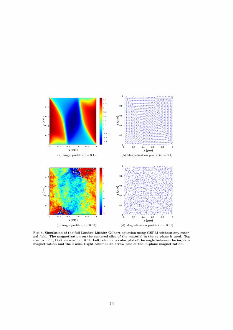
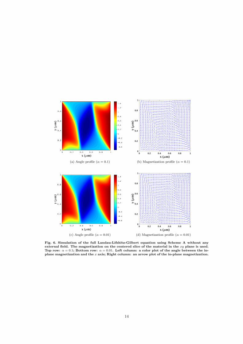
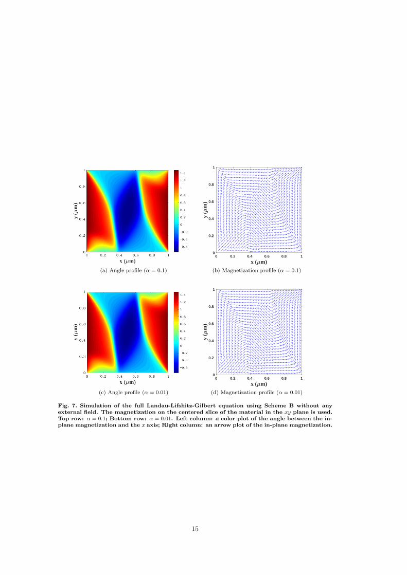
Following [18], we consider the full LLG equation with α = 0.1 and α = 0.01 and without

the external field. The initial state is m0 = (0, 1, 0) if x ∈ [0, Lx/5] ∪ [4Lx/5, Lx] and

m0 = (1, 0, 0) otherwise. The final time is 10 ns. In Figures 5 to 7, we present a color plot

of the angle between the in-plane magnetization and the x axis, and an arrow plot of the

in-plane magnetization for the original GSPM [15], Scheme A, and Scheme B, respectively.

In these figures, α = 0.1 is presented in the top row and α = 0.01 is presented in the bottom

row; a color plot of the angle between the in-palne magnetization and the x axis is presented

in the left column and an arrow plot of the in-plane magnetization is presented in the right

column.

5. Conclusion

In this paper, based on the original Gauss-Seidel projection methods, we present two

improved Gauss-Seidel projection methods with the first-order accuracy in time and the

second-order accuracy in space. The first method updates the gyromagnetic term and the

11

XXXXXXXXXXCPU time∆x

1/6 1/8 1/10 1/12 Reference


Table 5. Recorded CPU time in 3D with respect to the approximation error when only thespatial gridsize is varied with ∆x = ∆y = ∆z and ∆t = 1.0e− 09.

-50 -40 -30 -20 -10 0 10 20 30 40 50

0 H (mT)

-1

-0.8

-0.6

-0.4

-0.2

0

0.2

0.4

0.6

0.8

1

M/M

s

GSPM Scheme A Scheme B

Fig. 4. Comparison of hysteresis loops for GSPM, Scheme A and Scheme B. Profiles of the av-erage magnetization of these three methods are in quantitative agreements with approximatelythe same switch field 9 (±0.4) mT. The applied field is parallel to the x axis and the initial stateis the uniform state.

damping term simultaneously and follows by a projection step, which requires to solve heat

equations 5 times at each time step. The second method introduces two sets of approximate

solutions, where we update the gyromagnetic term and the damping term simultaneously for

one set of approximate solutions and apply the projection step to the other set of approximate

solutions in an alternating manner. Therefore, only 3 heat equations are needed to be solved

at each step. Compared to the original Gauss-Seidel projection method, which solves heat

equations 7 times at each step, savings of these two improved methods are about 2/7 and

4/7, which is verified by both 1D and 3D examples for the same accuracy requirement. In

addition, unconditional stability with respect to both the grid size and the damping parameter

is confirmed numerically. Application of both methods to a realistic material is also presented

with hysteresis loops and magnetization profiles.

Acknowledgments

This work is supported in part by the grants NSFC 21602149 (J. Chen), NSFC 11501399

(R. Du), the Hong Kong Research Grants Council (GRF grants 16302715, 16324416, 16303318

12

(a) Angle profile (α = 0.1)

0 0.2 0.4 0.6 0.8 1

x ( m)

0

0.2

0.4

0.6

0.8

1

y (

m)

(b) Magnetization profile (α = 0.1)

(c) Angle profile (α = 0.01)

0 0.2 0.4 0.6 0.8 1

x ( m)

0

0.2

0.4

0.6

0.8

1

y (

m)

(d) Magnetization profile (α = 0.01)

Fig. 5. Simulation of the full Landau-Lifshitz-Gilbert equation using GSPM without any exter-nal field. The magnetization on the centered slice of the material in the xy plane is used. Toprow: α = 0.1; Bottom row: α = 0.01. Left column: a color plot of the angle between the in-planemagnetization and the x axis; Right column: an arrow plot of the in-plane magnetization.

13


0 0.2 0.4 0.6 0.8 1

x ( m)

0

0.2

0.4

0.6

0.8

1

y (

m)



0 0.2 0.4 0.6 0.8 1

x ( m)

0

0.2

0.4

0.6

0.8

1

y (

m)


Fig. 6. Simulation of the full Landau-Lifshitz-Gilbert equation using Scheme A without anyexternal field. The magnetization on the centered slice of the material in the xy plane is used.Top row: α = 0.1; Bottom row: α = 0.01. Left column: a color plot of the angle between the in-plane magnetization and the x axis; Right column: an arrow plot of the in-plane magnetization.

14


0 0.2 0.4 0.6 0.8 1

x ( m)

0

0.2

0.4

0.6

0.8

1

y (

m)



0 0.2 0.4 0.6 0.8 1

x ( m)

0

0.2

0.4

0.6

0.8

1

y (

m)


Fig. 7. Simulation of the full Landau-Lifshitz-Gilbert equation using Scheme B without anyexternal field. The magnetization on the centered slice of the material in the xy plane is used.Top row: α = 0.1; Bottom row: α = 0.01. Left column: a color plot of the angle between the in-plane magnetization and the x axis; Right column: an arrow plot of the in-plane magnetization.

15

and NSFC-RGC joint research grant N-HKUST620/15) (X.-P. Wang), and the Innovation

Program for postgraduates in Jiangsu province via grant KYCX19 1947 (C. Xie).

References

[1] L. Landau, E. Lifshitz, On the theory of the dispersion of magetic permeability in ferromagnetic bodies,Phys. Z. Sowjetunion 8 (1935) 153–169.

[2] T. Gilbert, A lagrangian formulation of gyromagnetic equation of the magnetization field, Phys. Rev.100 (1955) 1243–1255.

[3] W. F. B. Jr., Micromagnetics, Interscience Tracts on Physics and Astronomy, 1963.[4] P. Sulem, C. Sulem, C. Bardos, On the continuous limit limit for a system of classical spins, Comm.

Math. Phys. 107 (1986) 431–454.[5] M. Struwe, On the evolution of harmonic maps in higher dimensions, J. Differential Geom. 28 (1988)

485–502.[6] I. Zutic, J. Fabian, S. Das Sarma, Spintronics: Fundamentals and applications, Rev. Mod. Phys. 76

(2004) 323–410.[7] M. Kruzik, A. Prohl, Recent developments in the modeling, analysis, and numerics of ferromagnetism,

SIAM Rev. 48 (2006) 439–483.[8] I. Cimrak, A survey on the numerics and computations for the Landau-Lifshitz equation of micromag-

netism, Arch. Comput. Methods Eng. 15 (2008) 277–309.[9] C. J. Garcıa-Cervera, Numerical micromagnetics: a review, Bol. Soc. Esp. Mat. Apl. 39 (2007) 103–135.

[10] A. Francois, J. Pascal, Convergence of a finite element discretization for the Landau-Lifshitz equationsin micromagnetism, Math. Models Methods Appl. Sci. 16 (2006) 299–316.

[11] A. Romeo, G. Finocchio, M. Carpentieri, L. Torres, G. Consolo, B. Azzerboni, A numerical solution ofthe magnetization reversal modeling in a permalloy thin film using fifth order runge-kutta method withadaptive step size control, Physica B. 403 (2008) 1163–1194.

[12] Y. H, H. N, Implicit solution of the Landau-Lifshitz-Gilbert equation by the Crank-Nicolson method,J. Magn. Soc. Japan 28 (2004) 924–931.

[13] S. Bartels, P. Andreas, Convergence of an implicit finite element method for the Landau-Lifshitz-Gilbertequation, SIAM J. Numer. Anal. 44 (2006) 1405–1419.

[14] A. Fuwa, T. Ishiwata, M. Tsutsumi, Finite difference scheme for the Landau-Lifshitz equation, JapanJ. Indust. Appl. Math. 29 (2012) 83–110.

[15] X. Wang, C. J. Garcıa-Cervera, W. E, A gauss-seidel projection method for micromagnetics simulations,J. Comput. Phys. 171 (2001) 357–372.

[16] W. E, X. Wang, Numerical methods for the Landau-Lisfshitz equation, SIAM J. Numer. Anal. 38 (2000)1647–1665.

[17] J. Chen, C. Wang, C. Xie, Convergence analysis of a second-order semi-implicit projection method forLandau-Lifshitz equation, arXiv 1902.09740 (2019).

[18] C. J. Garcıa-Cervera, W. E, Improved gauss-seidel projection method for micromagnetics simulations,IEEE Trans. Magn. 39 (2003) 1766–1770.

[19] I. Cimrak, Error estimates for a semi-implicit numerical scheme solving the Landau-Lifshitz equationwith an exchange field, IMA J. Numer. Anal. (2005) 611–634.

16

two improved gauss-seidel projection methods for landau ... · two improved gauss-seidel projection...

Documents