Mathematical Social Sciences 71 (2014) 12–19

Contents lists available at ScienceDirect

Mathematical Social Sciences

journal homepage: www.elsevier.com/locate/econbase

Two kinds of Pareto improvements of the economic system: Aninput–output analysis using the nonnegative matrices theoryLisheng ZengInstitute of Quantitative and Technical Economics, Chinese Academy of Social Sciences, 5 Jianguomennei Street, Beijing 100732, People’s Republic of China

h i g h l i g h t s

• Define the Pareto improvement of final output rate and input multiplier.• Define the Pareto improvement of value-added rate and output multiplier.• Give a sufficient condition for Pareto improvement of final output rate and input multiplier.• Give a sufficient condition for Pareto improvement of value-added rate and output multiplier.• Define the partitional row and column indicator sets for a reducible nonnegative matrix.

a r t i c l e i n f o

Article history:Received 20 February 2013Received in revised form28 September 2013Accepted 7 April 2014Available online 18 April 2014

a b s t r a c t

This paper clearly reveals the economic meanings of final output rate, input multiplier, value-added rate,and output multiplier. Applying the output adjustment model and the price adjustment model as well asnonnegativematrices theorywe find that if thematrix of intermediate output (or input) coefficients has atleast one non-final (or non-initial) class then (i) an adjustment of output system enables the final outputrates of whole or part sectors corresponding to the non-final classes to rise, the inputmultipliers of wholeor part sectors corresponding to the non-final classes to decrease, and all other sectoral final output ratesand input multipliers to be fixed, which is one kind of Pareto improvement of the economic system; (ii)the adaptation of price system enables the value-added rates of whole or part sectors corresponding tothe non-initial classes to rise, the output multipliers of whole or part sectors corresponding to the non-initial classes to decrease, and all other sectoral value-added rates and outputmultipliers to be unchanged,which is another kind of Pareto improvement of the economic system. We respectively give a sufficientcondition for the two kinds of Pareto improvements. A numerical example verifies these results.

© 2014 Elsevier B.V. All rights reserved.

1. Introduction

Brown et al. (1973) and Brown and Licari (1977) introducedthe ‘‘price adjustment model’’ in order to research the socialistprice mechanism. Dietzenbacher (1997) analyzed the relationshipbetween Ghosh’s ‘‘supply-driven’’ input–output model and Leon-tief’s traditional ‘‘demand-driven’’ input–output model, where theprice adjustmentmodel (seeDietzenbacher, 1997, formula (9)) andthe output adjustment model in value terms (see Dietzenbacher,1997, formula (12)) were included, though he did not use suchterminologies. Zeng (2008) established the physical output adjust-mentmodel, discussed output adjustmentmodel and price adjust-ment model as well as their basic natures, and revealed the effectsof changes in outputs on final output rates and input multipliers

E-mail address: zengls@cass.org.cn.

http://dx.doi.org/10.1016/j.mathsocsci.2014.04.0010165-4896/© 2014 Elsevier B.V. All rights reserved.

and the effects of changes in prices on value-added rates and out-put multipliers. Zeng (2010) discovered the equivalent conditionsthat all sectoral final output rates equal their respective sectoralvalue-added rates and that all sectoral inputmultipliers equal theirrespective sectoral output multipliers.

From Zeng (2008, 2010), the accommodation of output systemcan alter twokinds of indicators: final output rates and inputmulti-pliers; also the adaptation of price system can alter two kinds of in-dicators: value-added rates and outputmultipliers. However, whatare the comprehensive economic meanings of the four kinds of in-dicators? Only the input multiplier and the output multiplier arepartly explained via Miller and Blair (1985, Chapter 9), the value-added rate is preliminarily interpreted by Zeng (2008), and yet thefinal output rate is not clarified.

Via Zeng (2008, 2010), an adjustment of output system enablessome sectoral final output rates to rise and all others to be constant,and/or some sectoral input multipliers to decrease and all others

L. Zeng / Mathematical Social Sciences 71 (2014) 12–19 13

to be fixed. Nevertheless, how is the output system adjusted? Zeng(2008, 2010) does not present the corresponding method thoughthe proof of Zeng (2008, Theorem 1) gives us an inkling. Besides,which sectoral final output rates can be risen? Which sectoralinput multipliers can be decreased? Zeng (2008, 2010) does notdiscuss these problems. Similarly, the adaptation of price systemenables some sectoral value-added rates to rise and all others tobe unchanged, and/or some sectoral outputmultipliers to decreaseand all others to be constant. However, Zeng (2008, 2010) does notoffer thematchingmethod of adapting the price system.Moreover,which sectoral value-added rates can be risen? Which sectoraloutput multipliers can be decreased? Zeng (2008, 2010) does notexpound these problems.

Based on Zeng (2008, 2010) this paper will solve the aforesaidproblems, which will be very useful to improve the four kinds ofindicators of the economic system and to develop the close rela-tionship between input–output economic theory and nonnegativematrices theory, which are just the main purposes of this paper.

First we shall completely give the economic meanings of thefour kinds of indicators. Also we shall definitely indicate that byadjusting the output system some sectoral final output rates arerisen and all others are fixed, and some sectoral input multipli-ers are decreased and all others are unchanged, this is one kind ofPareto improvement of the economic system, which can be calledthe Pareto improvement of final output rate and input multiplier, andthat by adapting the price system some sectoral value-added ratesare risen and all others are constant, and some sectoral outputmultipliers are decreased and all others are fixed, this is anotherkind of Pareto improvement of the economic system, which can becalled the Pareto improvement of value-added rate and output mul-tiplier. The two kinds of Pareto improvements are dual. Next weshall present the concrete method of adjusting the output system,which is really a sufficient condition for the Pareto improvementof final output rate and input multiplier. At the same time, the sec-toral types of final output rates to be risen and of input multipli-ers to be decreased are roughly divided by the non-final class(es)of the matrix of intermediate output coefficients. Dually, we shalloffer the concrete method of adapting the price system, which isactually a sufficient condition for the Pareto improvement of value-added rate and output multiplier. At the same time, the sectoraltypes of value-added rates to be risen and of output multipliers tobe decreased are roughly divided by the non-initial class(es) of thematrix of intermediate input coefficients. Finallywe shall verify theabove theory and approaches via a numerical example.

The paper is organized as follows.In Section 2, the economic meanings of the four kinds of indi-

cators are revealed. It is indicated that the higher the final outputrate is, the smaller the input multiplier is, which is more benefi-cial to the economic system, and that the higher the value-addedrate is, the smaller the output multiplier is, which is more prof-itable to the economic system. By Definition 1 we establish fournew concepts of the partitional row (or column) indicator sets cor-responding to non-final (or non-initial) class(es) and to final (orinitial) class(es) for a Frobenius normal form of a reducible non-negative matrix. Definition 1 and Theorem 1 are the indispensablemathematical foundations of this paper.

In Section 3, a new concept of the Pareto improvement of finaloutput rate and input multiplier is founded. Dually, a new conceptof the Pareto improvement of value-added rate and output multi-plier is presented.

In Section 4, the concrete approach to the Pareto improvementof final output rate and input multiplier is expounded. Dually, theconcrete approach to the Pareto improvement of value-added rateand outputmultiplier is elucidated. Theorems 2 and 3 are the cores.

In Section 5, a numerical example illustrates and verifies themain results, where the two kinds of Pareto improvements of theeconomic system are simulated.

2. Preliminary analysis and concepts

2.1. Notations and terminologies

For the general notations and terminologies, let logical nota-tions ∃, ∀, ∧, ∨, and ⇔ represent existence, arbitrariness, con-junction, disjunction, and equivalence, respectively. Via Γ ⇒ Ω ,we denote that Γ implies Ω . The set notations ∈, ∪, and ∩ standfor belong, union of sets, and intersection of sets, respectively. Theempty set is indicated by φ. Let 0 be zero, a zero vector or zero ma-trix. A vector or matrix M > 0 means that M is semipositive, i.e.every entry of M is nonnegative, and M = 0. A vector or matrixM ≫ 0 implies that M is positive, viz. every element of M is posi-tive. A vector ormatrixM is called strictly semipositive, ifM > 0 andat least one entry is zero. Evidently,M is semipositive if and only ifM is positive or strictly semipositive. By M t we indicate the trans-pose of vector or matrixM . Let ρ(M) represent the spectral radiusof amatrixM . Let H = diag(H) = diag(h1, h2, . . . , hn) be the diag-onal matrix with h1, h2, . . . , hn as its main diagonal entries, whereH is a column or row vector. The unit matrix is represented via I .The unit column vector E = (1, 1, . . . , 1)t .

Furthermore, let q ≫ 0 be a column vector of physical grossoutputs; p ≫ 0, a row vector of prices; X = pq ≫ 0, a column vec-tor of gross output values, and thus X t

≫ 0, a row vector of grossinput values; x = EtX = X tE > 0, the sumof all sectoral gross out-put values or gross input values; F = (fi)n×1 > 0, a column vectorofmonetary final demands (or final output values); Y = X−1F > 0,a column vector of final output rates; V = (vj)1×n > 0, a row vec-tor of values-added (or primary input values); R = V X−1 > 0, arow vector of value-added rates; Z > 0, a monetary transactionmatrix for the intermediate products; ZE > 0, a column vectorof intermediate output values; EtZ > 0, a row vector of interme-diate input values; w = EtZE > 0, the sum of all sectoral in-termediate output values or intermediate input values; A > 0, amatrix of physical intermediate input coefficients; A = X−1Z =

(aij)n×n > 0, a matrix of intermediate output coefficients; AE > 0,a column vector of intermediate output rates; B = (I − A)−1

=

(bij)n×n > 0, a Ghosh inverse matrix; G = BE = (gi)n×1 ≫ 0,a column vector of input multipliers; A = ZX−1

= (aij)n×n > 0,a matrix of monetary intermediate input coefficients; EtA > 0, arow vector of intermediate input rates; B = (I−A)−1

= (bij)n×n >0, a monetary Leontief inverse matrix; D = EtB = (dj)1×n ≫ 0, arow vector of output multipliers; where ρ(A) = ρ(A) = ρ(A) <

1, A = q−1Aq = X−1AX, B = X−1BX , and A = pAp−1 (see alsoMiller and Blair, 1985, Chapter 9). Let Q ≫ 0 be a column vectorof output adjustment coefficients; P ≫ 0, a row vector of price ad-justment coefficients; the superscript # correspond to the newout-put system; the superscript * correspond to the new price system;where A#

= Q−1AQ , B#= Q−1BQ , A∗

= PAP−1, and B∗= PBP−1

(see Zeng, 2008).

2.2. Meanings of final output rate and input multiplier

It is known that the intermediate output rate plus the final out-put rate equals 1, namely, AE+Y = E. The intermediate output is tobe expended for producing the final output. As compared with theintermediate output, the final output is the only product that canbe of material benefit to the people. Also, the final purpose of pro-duction is exactly to satisfy the people’s final material demand, i.e.to gain the final output. Thus the higher the final output rate is (viz.the lower the intermediate output rate is), the more beneficial theachievement of the ultimate goal of production is. From this view-point, therefore, a sectoral final output rate represents this sectoraleconomic efficiency about final output, and the column vector of

14 L. Zeng / Mathematical Social Sciences 71 (2014) 12–19

final output rates stands for the economic systemic integrative pro-duction efficiency about the final output.

It is also known that a sectoral input multiplier measures therate of change of the sum of all sectoral gross input values ofthe economy with respect to this sectoral primary input value (orvalue-added), namely, gi =

nk=1 bik = ∂x/∂vi (i = 1, 2, . . . , n).

From this formula and x = X tE = (EtZ + V )E = EtZE + VE =

w +n

k=1 vk, we can obtain

gi = (∂w/∂vi) + 1 (i = 1, 2, . . . , n), (1)

i.e. a sectoral input multiplier equals the rate of change of thesum of all sectoral intermediate input values of the economy withrespect to this sectoral primary input value plus 1.

Since 1 is a constant, via (1), a sectoral input multiplier reflectsmainly the rate of change of the sum of all sectoral intermediateinput values of the economy with respect to this sectoral primaryinput value. Because every sectoral intermediate input value isthe raw material cost spent by this sector, the sum of all sectoralintermediate input values equals the total raw material costconsumed by the economic system. Accordingly a sectoral inputmultiplier reveals chiefly the economic systemic total cost relativeto this sectoral primary input value, and the column vector of inputmultipliers shows mainly the economic systemic integrative totalcost relative to primary input. Besides, every element in B = (I −

A)−1 is a function of n × n elements in A. Similarly to Zeng (2001,formula (3)), we have (∂ bkr/∂ aij) ≥ 0 (i, j, k, r = 1, 2, . . . , n).This means that the change directions of elements in B and ofelements in A are the same. Hence the following five statementsare apparently equivalent:

(i) the final output rate is higher;(ii) the intermediate output rate is lower;(iii) the elements in thematrix of intermediate output coefficients

are smaller;(iv) the elements in the Ghosh inverse matrix are smaller;(v) the components in the column vector of input multipliers are

smaller.

From the above paragraphs, the input multiplier is smaller, whichmeans that the economic systemic total cost relative to primaryinput is lower,which alsomeans that the final output rate is higher,namely, the economic efficiency about final output is higher,whichis more advantageous to the achievement of the final aim ofproduction.

2.3. Meanings of value-added rate and output multiplier

It is known that the intermediate input rate plus the value-added rate equals 1, namely, EtA+ R = Et . The intermediate inputvalue is the rawmaterial cost expended. The value-added containsmainly wage and profit. As compared with the intermediate inputvalue, the value-added is only new creative value. For every sector,only if it creates the value-added can it gain economic returnsand develop production. Hence the higher the value-added rateis (i.e. the lower the intermediate input rate is), the higher therelative return is, and themore profitable the normal developmentof production is. From this viewpoint, therefore, a sectoral value-added rate reflects approximately this sectoral economic returnrate, and the row vector of value-added rates nearly displays theeconomic systemic integrative return rate.

It is also known that a sectoral output multiplier appraises therate of change of the sum of all sectoral gross output values ofthe economy with respect to this sectoral final output value, i.e.dj =

nk=1 bkj = ∂x/∂ fj (j = 1, 2, . . . , n). Dually to (1), via the

same principle we can prove

dj = (∂w/∂ fj) + 1 (j = 1, 2, . . . , n), (2)

viz. a sectoral output multiplier equals the rate of change of thesumof all sectoral intermediate output values of the economywithrespect to this sectoral final output value plus 1.

From (2), a sectoral output multiplier reflects chiefly the rateof change of the sum of all sectoral intermediate output valuesof the economy with respect to this sectoral final output value.Because the sum of all sectoral intermediate output values equalsthe sum of all sectoral intermediate input values, which is equal tothe total rawmaterial cost spent by the economic system, a sectoraloutput multiplier shows mainly the economic systemic total costrelative to this sectoral final output, and the row vector of outputmultipliers reveals chiefly the economic systemic integrative totalcost relative to final output. Moreover, dually to Section 2.2 thefollowing five statements are also equivalent:

(i) the value-added rate is higher;(ii) the intermediate input rate is lower;(iii) the elements in the matrix of monetary intermediate input

coefficients are smaller;(iv) the elements in the monetary Leontief inverse matrix are

smaller;(v) the components in the row vector of output multipliers are

smaller.

By the above contents, the output multiplier is smaller, whichmeans that the economic systemic total cost relative to final out-put is lower, which also means that the value-added rate is higher,namely, the economic return rate is higher, which is more prof-itable to the economic development.

2.4. Necessary mathematical definition and theorem

For an arbitrary nonnegative n × n matrix T , we can alwaysexpress it by a normal form. Assumewithout loss of generality thatT itself is a lower triangular Frobenius normal form, i.e.

T =

T11 0...

. . .

Tr1 · · · Trr

, (3)

where 1 ≤ r ≤ n. When T is reducible (viz. r ≥ 2) we give thefollowing definition.

Definition 1. Corresponding to (3), let the sets D+ = d | Tde > 0,∃ e < d,D0 = d | Tde = 0, ∀e < d , E+ = e | Tde > 0, ∃ d > e ,and E0 = e | Tde = 0, ∀d > e . Then D+ and D0 ∪ 1 are respec-tively called the partitional row indicator set corresponding to thenon-final class(es) for T and the partitional row indicator set corre-sponding to the final class(es) for T ; E+ and E0 ∪ r are respectivelycalled the partitional column indicator set corresponding to the non-initial class(es) for T and the partitional column indicator set corre-sponding to the initial class(es) for T .

From Definition 1, we can clearly obtain D+ ∪ D0 = 2, . . . ,r, E+ ∪ E0 = 1, . . . , r − 1, and D+ ∩ D0 = φ = E+ ∩ E0.

Theorem 1. Let T be a nonnegative matrix of order n, µ > ρ(T ),and L = (µI − T )−1. Then

(i) (3) is a lower triangular Frobenius normal form of T if and onlyif

L =

L11 0...

. . .

Lr1 · · · Lrr

L. Zeng / Mathematical Social Sciences 71 (2014) 12–19 15

is a lower triangular Frobenius normal form of L, where

Lii = (µIi − Tii)−1≫ 0 (i = 1, . . . , r), (4)

Li+1i = (µIi+1 − Ti+1i+1)−1Ti+1i(µIi − Tii)−1

(i = 1, . . . , r − 1), (5)

Lji = (µIj − Tjj)−1Nji(µIi − Tii)−1

(j = 3, . . . , r, i = 1, . . . , j − 2), (6)

Nji = Tji +j−1−ik=1

j−k

b1=i+1

· · ·

j−1bk=bk−1+1

Tjbk

×

1m=k

LbmbmTbmbm−1

, b0 = i < j − 1, (7)

Ii is the appropriate identity matrix for i = 1, . . . , r;(ii) in (5), Li+1i = 0 ⇔ Ti+1i = 0; Li+1i ≫ 0 ⇔ Ti+1i > 0;(iii) in (6) and (7),

Tji Tji+1 · · · Tjj−1

= 0 ∨

Ti+1i

...Tj−1iTji

= 0

⇒ Nji = 0 ⇔ Lji = 0 ⇒ Tji = 0;

Tji > 0 ⇒ Lji ≫ 0 ⇔ Nji > 0

⇒

Tji Tji+1 · · · Tjj−1

> 0 ∧

Ti+1i

...Tj−1iTji

> 0

;

(iv) the partitional row indicator sets corresponding to non-finalclass(es) and final class(es) for T are respectively equal to thepartitional row indicator sets corresponding to non-final class(es)and final class(es) for L; the partitional column indicator setscorresponding to non-initial class(es) and initial class(es) for Tare respectively equal to the partitional column indicator setscorresponding to non-initial class(es) and initial class(es) for L.

The proof of Theorem 1 is delegated to Appendix.

Remark 1. Conclusion (iv) in Theorem 1 shows that (i) if T hasthe non-final or non-initial class(es) then L has also the same non-final or non-initial class(es), and vice versa, namely, the non-finalclasses of T and L are one-to-one, and the non-initial classes of Tand L are also one-to-one; (ii) the final classes of T and L are one-to-one, and the initial classes of T and L are also one-to-one. Obviously,Theorem 1 develops or improves Zeng (2008, Theorem A2).

3. Two kinds of Pareto improvements

3.1. Pareto improvement of final output rate and input multiplier

Since A = q−1Aq, the matrix A alters if and only if q changeswhen A is constant. Therefore, Y = (I−A)E orG = (I−A)−1E altersif and only if q changes when we assume that A is fixed. That is, wecan alter every sectoral final output rate (i.e. the economic systemicintegrative production efficiency about final output) or everysectoral input multiplier (viz. the economic systemic integrativetotal cost relative to primary input) by adjusting the output system.

Based on part (i) in Zeng (2008, Proposition 3), parts (a) and(c) in Zeng (2008, Theorem 1), and conclusions (i) and (ii) in Zeng(2008, Corollary 3), we shall reveal that if the matrix of intermedi-ate output coefficients has at least one non-final class then an ad-justment of output system enables the final output rates of wholeor part sectors corresponding to the non-final classes to rise, the in-put multipliers of whole or part sectors corresponding to the non-

final classes to decrease, and all other sectoral final output ratesand input multipliers to be fixed. Under this condition, therefore,ifwe adjust the output system then the economic systemic integra-tive production efficiency about final output is certainly risen andthe economic systemic integrative total cost relative to primary in-put is surely decreased, because at least one sectoral final outputrate is risen, at least one sectoral inputmultiplier is decreased; andat least one sectoral final output rate is constant, at least one sec-toral input multiplier is fixed; and there is no sector whose finaloutput rate is fallen or input multiplier is increased. This is just thePareto improvement of final output rate and input multiplier.

3.2. Pareto improvement of value-added rate and output multiplier

Since A = pAp−1, the matrix A alters if and only if p changeswhen A is unchanged. Hence,R = Et(I−A) orD = Et(I−A)−1 altersif and only if p changes when we assume that A is fixed. Namely,we can alter every sectoral value-added rate (i.e. the economic sys-temic integrative return rate) or every sectoral output multiplier(viz. the economic systemic integrative total cost relative to finaloutput) via adapting the price system.

Based on part (ii) in Zeng (2008, Proposition 3), parts (b) and(c) in Zeng (2008, Theorem 1), and conclusions (iii) and (iv) in Zeng(2008, Corollary 3),we shall show that if thematrix of intermediateinput coefficients has at least one non-initial class then the accom-modation of price system enables the value-added rates of wholeor part sectors corresponding to the non-initial classes to rise, theoutput multipliers of whole or part sectors corresponding to thenon-initial classes to decrease, and all other sectoral value-addedrates and output multipliers to be constant. Under this condition,therefore, if we accommodate the price system then the economicsystemic integrative return rate is certainly risen and the economicsystemic integrative total cost relative to final output is surely de-creased, because at least one sectoral value-added rate is risen, atleast one sectoral output multiplier is decreased; and at least onesectoral value-added rate is unchanged, at least one sectoral out-put multiplier is fixed; and there is no sector whose value-addedrate is fallen or output multiplier is increased. This is exactly thePareto improvement of value-added rate and output multiplier.

4. Approaches to two kinds of Pareto improvements

Suppose that an economic system comprises n sectors, whosematrix of intermediate output coefficients, A, has at least onenon-final class, viz. whose matrix of monetary intermediate inputcoefficients,A, has at least onenon-initial class. Thenwe can alwayspermute the two matrices into the lower triangular Frobeniusnormal forms by a permutationmatrix. Accordinglywe can assumewithout loss of generality that A and A themselves are the lowertriangular Frobenius normal forms. Namely

A =

A11 0A21 A22...

.... . .

Ar1 Ar2 · · · Arr

,

A = X AX−1=

A11 0A21 A22...

.... . .

Ar1 Ar2 · · · Arr

,

(8)

where 2 ≤ r ≤ n, and the submatrices obviously satisfy Ade > 0 ⇔

Ade > 0, d = 1, 2, . . . , r, e = 1, . . . , d; Ade = 0 ⇔ Ade = 0, d =

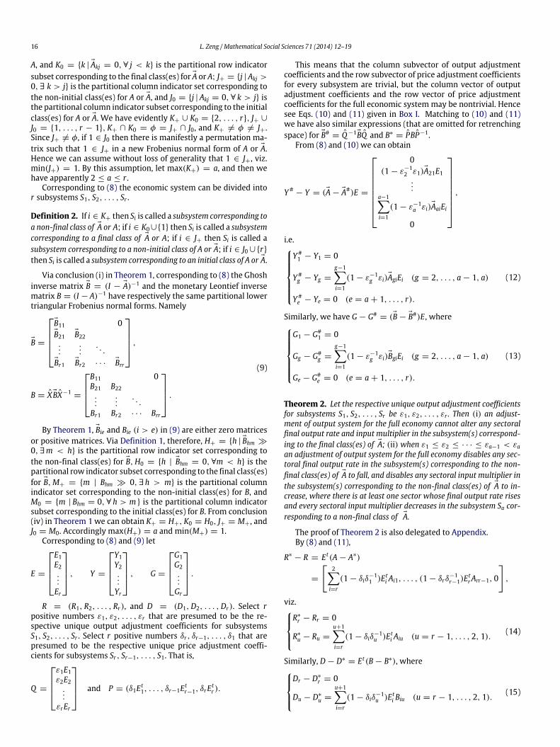
2, . . . , r, e = 1, . . . , d − 1.Via Definition 1, K+ = k | Akj > 0, ∃ j < k is the partitional

row indicator set corresponding to the non-final class(es) for A or

16 L. Zeng / Mathematical Social Sciences 71 (2014) 12–19

A, and K0 = k | Akj = 0, ∀ j < k is the partitional row indicatorsubset corresponding to the final class(es) for A or A; J+ = j | Akj >0, ∃ k > j is the partitional column indicator set corresponding tothe non-initial class(es) for A or A, and J0 = j | Akj = 0, ∀ k > j isthe partitional column indicator subset corresponding to the initialclass(es) for A or A. We have evidently K+ ∪ K0 = 2, . . . , r, J+ ∪

J0 = 1, . . . , r − 1, K+ ∩ K0 = φ = J+ ∩ J0, and K+ = φ = J+.Since J+ = φ, if 1 ∈ J0 then there is manifestly a permutation ma-trix such that 1 ∈ J+ in a new Frobenius normal form of A or A.Hence we can assume without loss of generality that 1 ∈ J+, viz.min(J+) = 1. By this assumption, let max(K+) = a, and then wehave apparently 2 ≤ a ≤ r .

Corresponding to (8) the economic system can be divided intor subsystems S1, S2, . . . , Sr .

Definition 2. If i ∈ K+ then Si is called a subsystem corresponding toa non-final class of A or A; if i ∈ K0∪1 then Si is called a subsystemcorresponding to a final class of A or A; if i ∈ J+ then Si is called asubsystem corresponding to a non-initial class of A or A; if i ∈ J0 ∪rthen Si is called a subsystem corresponding to an initial class of A or A.

Via conclusion (i) in Theorem 1, corresponding to (8) the Ghoshinverse matrix B = (I − A)−1 and the monetary Leontief inversematrix B = (I − A)−1 have respectively the same partitional lowertriangular Frobenius normal forms. Namely

B =

B11 0B21 B22...

.... . .

Br1 Br2 · · · Brr

,

B = X BX−1=

B11 0B21 B22...

.... . .

Br1 Br2 · · · Brr

.

(9)

By Theorem 1, Bie and Bie (i > e) in (9) are either zero matricesor positive matrices. Via Definition 1, therefore, H+ = h | Bhm ≫

0, ∃m < h is the partitional row indicator set corresponding tothe non-final class(es) for B,H0 = h | Bhm = 0, ∀m < h is thepartitional row indicator subset corresponding to the final class(es)for B,M+ = m | Bhm ≫ 0, ∃ h > m is the partitional columnindicator set corresponding to the non-initial class(es) for B, andM0 = m | Bhm = 0, ∀ h > m is the partitional column indicatorsubset corresponding to the initial class(es) for B. From conclusion(iv) in Theorem 1 we can obtain K+ = H+, K0 = H0, J+ = M+, andJ0 = M0. Accordingly max(H+) = a and min(M+) = 1.

Corresponding to (8) and (9) let

E =

E1E2...Er

, Y =

Y1Y2...Yr

, G =

G1G2...Gr

.

R = (R1, R2, . . . , Rr), and D = (D1,D2, . . . ,Dr). Select rpositive numbers ε1, ε2, . . . , εr that are presumed to be the re-spective unique output adjustment coefficients for subsystemsS1, S2, . . . , Sr . Select r positive numbers δr , δr−1, . . . , δ1 that arepresumed to be the respective unique price adjustment coeffi-cients for subsystems Sr , Sr−1, . . . , S1. That is,

Q =

ε1E1ε2E2

...εrEr

and P = (δ1Et1, . . . , δr−1Et

r−1, δrEtr ).

This means that the column subvector of output adjustmentcoefficients and the row subvector of price adjustment coefficientsfor every subsystem are trivial, but the column vector of outputadjustment coefficients and the row vector of price adjustmentcoefficients for the full economic system may be nontrivial. Hencesee Eqs. (10) and (11) given in Box I. Matching to (10) and (11)we have also similar expressions (that are omitted for retrenchingspace) for B#

= Q−1BQ and B∗= PBP−1.

From (8) and (10) we can obtain

Y#− Y = (A − A#)E =

0(1 − ε−1

2 ε1)A21E1...

a−1i=1

(1 − ε−1a εi)AaiEi

0

,

i.e.Y#1 − Y1 = 0

Y#g − Yg =

g−1i=1

(1 − ε−1g εi)AgiEi (g = 2, . . . , a − 1, a)

Y#e − Ye = 0 (e = a + 1, . . . , r).

(12)

Similarly, we have G − G#= (B − B#)E, where

G1 − G#1 = 0

Gg − G#g =

g−1i=1

(1 − ε−1g εi)BgiEi (g = 2, . . . , a − 1, a)

Ge − G#e = 0 (e = a + 1, . . . , r).

(13)

Theorem 2. Let the respective unique output adjustment coefficientsfor subsystems S1, S2, . . . , Sr be ε1, ε2, . . . , εr . Then (i) an adjust-ment of output system for the full economy cannot alter any sectoralfinal output rate and input multiplier in the subsystem(s) correspond-ing to the final class(es) of A; (ii) when ε1 ≤ ε2 ≤ · · · ≤ εa−1 < εaan adjustment of output system for the full economy disables any sec-toral final output rate in the subsystem(s) corresponding to the non-final class(es) of A to fall, and disables any sectoral input multiplier inthe subsystem(s) corresponding to the non-final class(es) of A to in-crease, where there is at least one sector whose final output rate risesand every sectoral input multiplier decreases in the subsystem Sa cor-responding to a non-final class of A.

The proof of Theorem 2 is also delegated to Appendix.By (8) and (11),

R∗− R = Et(A − A∗)

=

2

i=r

(1 − δiδ−11 )Et

i Ai1, . . . , (1 − δrδ−1r−1)E

trArr−1, 0

,

viz.R∗

r − Rr = 0

R∗

u − Ru =

u+1i=r

(1 − δiδ−1u )Et

i Aiu (u = r − 1, . . . , 2, 1). (14)

Similarly, D − D∗= Et(B − B∗), where

Dr − D∗

r = 0

Du − D∗

u =

u+1i=r

(1 − δiδ−1u )Et

i Biu (u = r − 1, . . . , 2, 1). (15)

L. Zeng / Mathematical Social Sciences 71 (2014) 12–19 17

0)

1)

A#= Q−1AQ =

A11 0ε−12 ε1A21 A22

......

. . . 0ε−1a−1ε1Aa−11 ε−1

a−1ε2Aa−12 · · · Aa−1a−1

ε−1a ε1Aa1 ε−1

a ε2Aa2 · · · ε−1a εa−1Aaa−1 Aaa

Aa+1a+1 0

0. . .

0 Arr

, (1

A∗= PAP−1

=

A11 0

δ2δ−11 A21 A22...

.... . .

δr−1δ−11 Ar−11 δr−1δ

−12 Ar−12 · · · Ar−1r−1

δrδ−11 Ar1 δrδ

−12 Ar2 · · · δrδ

−1r−1Arr−1 Arr

. (1

Box I.

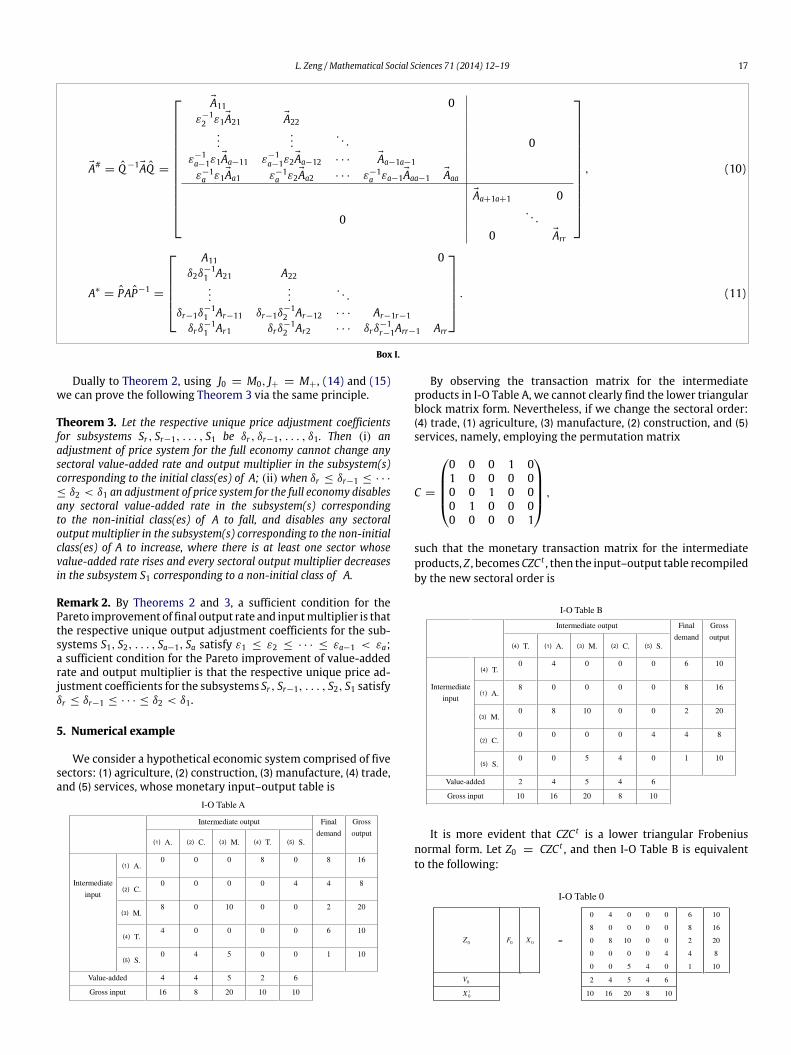
Dually to Theorem 2, using J0 = M0, J+ = M+, (14) and (15)we can prove the following Theorem 3 via the same principle.

Theorem 3. Let the respective unique price adjustment coefficientsfor subsystems Sr , Sr−1, . . . , S1 be δr , δr−1, . . . , δ1. Then (i) anadjustment of price system for the full economy cannot change anysectoral value-added rate and output multiplier in the subsystem(s)corresponding to the initial class(es) of A; (ii) when δr ≤ δr−1 ≤ · · ·

≤ δ2 < δ1 an adjustment of price system for the full economy disablesany sectoral value-added rate in the subsystem(s) correspondingto the non-initial class(es) of A to fall, and disables any sectoraloutput multiplier in the subsystem(s) corresponding to the non-initialclass(es) of A to increase, where there is at least one sector whosevalue-added rate rises and every sectoral output multiplier decreasesin the subsystem S1 corresponding to a non-initial class of A.

Remark 2. By Theorems 2 and 3, a sufficient condition for thePareto improvement of final output rate and inputmultiplier is thatthe respective unique output adjustment coefficients for the sub-systems S1, S2, . . . , Sa−1, Sa satisfy ε1 ≤ ε2 ≤ · · · ≤ εa−1 < εa;a sufficient condition for the Pareto improvement of value-addedrate and output multiplier is that the respective unique price ad-justment coefficients for the subsystems Sr , Sr−1, . . . , S2, S1 satisfyδr ≤ δr−1 ≤ · · · ≤ δ2 < δ1.

5. Numerical example

We consider a hypothetical economic system comprised of fivesectors: (1) agriculture, (2) construction, (3)manufacture, (4) trade,and (5) services, whose monetary input–output table is

By observing the transaction matrix for the intermediateproducts in I-O Table A, we cannot clearly find the lower triangularblock matrix form. Nevertheless, if we change the sectoral order:(4) trade, (1) agriculture, (3) manufacture, (2) construction, and (5)services, namely, employing the permutation matrix

C =

0 0 0 1 01 0 0 0 00 0 1 0 00 1 0 0 00 0 0 0 1

,

such that the monetary transaction matrix for the intermediateproducts, Z , becomesCZC t , then the input–output table recompiledby the new sectoral order is

It is more evident that CZC t is a lower triangular Frobeniusnormal form. Let Z0 = CZC t , and then I-O Table B is equivalentto the following:

18 L. Zeng / Mathematical Social Sciences 71 (2014) 12–19

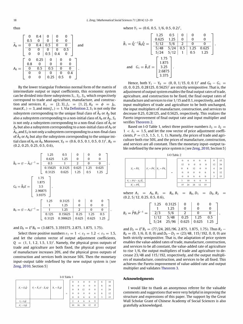
thus

A0 =

0 0.4 0 0 00.5 0 0 0 00 0.4 0.5 0 00 0 0 0 0.50 0 0.5 0.4 0

and

A0 =

0 0.25 0 0 00.8 0 0 0 00 0.5 0.5 0 00 0 0 0 0.40 0 0.25 0.5 0

.

By the lower triangular Frobenius normal form of the matrix ofintermediate output or input coefficients, this economic systemcan be divided into three subsystems S1, S2, S3, which respectivelycorrespond to trade and agriculture, manufacture, and construc-tion and services. K+ = 2, 3, J+ = 1, 2, K0 = φ = J0,max(K+) = 3, and min(J+) = 1. Via Definition 2, S1 is not only thesubsystem corresponding to the unique final class of A0 or A0 butalso a subsystem corresponding to a non-initial class of A0 or A0, S2is not only a subsystem corresponding to a non-final class of A0 orA0 but also a subsystem corresponding to a non-initial class of A0 orA0, and S3 is not only a subsystemcorresponding to a non-final classof A0 or A0 but also the subsystem corresponding to the unique ini-tial class of A0 or A0. Moreover, Y0 = (0.6, 0.5, 0.1, 0.5, 0.1)t , R0 =

(0.2, 0.25, 0.25, 0.5, 0.6),

B0 = (I − A0)−1

=

1.25 0.5 0 0 00.625 1.25 0 0 00.5 1 2 0 0

0.15625 0.3125 0.625 1.25 0.6250.3125 0.625 1.25 0.5 1.25

,

G0 = B0E =

1.751.8753.5

2.968753.9375

,

B0 = (I − A0)−1

=

1.25 0.3125 0 0 01 1.25 0 0 01 1.25 2 0 0

0.125 0.15625 0.25 1.25 0.50.3125 0.390625 0.625 0.625 1.25

,

and D0 = EtB0 = (3.6875, 3.359375, 2.875, 1.875, 1.75).Select three positive numbers ε1 = 1 < ε2 = 1.2 < ε3 = 1.5,

and let the column vector of output adjustment coefficients,Q = (1, 1, 1.2, 1.5, 1.5)t . Namely, the physical gross outputs oftrade and agriculture are both fixed, the physical gross outputof manufacture increases 20%, and the physical gross outputs ofconstruction and services both increase 50%. Then the monetaryinput–output table redefined by the new output system is (seeZeng, 2010, Section 5)

where Y1 = (0.6, 0.5, 1/6, 0.5, 0.2)t ,

B1 = Q−1B0Q =

1.25 0.5 0 0 00.625 1.25 0 0 05/12 5/6 2 0 05/48 5/24 0.5 1.25 0.6255/24 5/12 1 0.5 1.25

,

and G1 = B1E =

1.751.8753.25

2.68753.375

.

Hence, both Y1 − Y0 = (0, 0, 1/15, 0, 0.1)t and G0 − G1 =

(0, 0, 0.25, 0.28125, 0.5625)t are strictly semipositive. That is, theadjustment of output systemenables the final output rates of trade,agriculture, and construction to be fixed, the final output rates ofmanufacture and services to rise 1/15 and0.1, respectively, and theinput multipliers of trade and agriculture to be both unchanged,the input multipliers of manufacture, construction, and services todecrease 0.25, 0.28125, and 0.5625, respectively. This realizes thePareto improvement of final output rate and input multiplier andverifies Theorem 2.

Based on I-O Table 1, select three positive numbers δ3 = δ2 =

1 < δ1 = 1.5, and let the row vector of price adjustment coeffi-cients, P = (1.5, 1.5, 1, 1, 1). Namely, the prices of trade and agri-culture both rise 50%, and the prices of manufacture, construction,and services are all constant. Then the monetary input–output ta-ble redefined by the newprice system is (see Zeng, 2010, Section 5)

where A1 = A0, R1 = R0, B1 = B0,D1 = D0, R2 =

(0.2, 5/12, 0.25, 0.5, 0.6),

B2 = PB1P−1=

1.25 0.3125 0 0 01 1.25 0 0 0

2/3 5/6 2 0 01/12 5/48 0.25 1.25 0.55/24 25/96 0.625 0.625 1.25

,

and D2 = EtB2 = (77/24, 265/96, 2.875, 1.875, 1.75). Thus R2 −

R0 = (0, 1/6, 0, 0, 0) andD0−D2 = (23/48, 115/192, 0, 0, 0) areboth strictly semipositive. That is, the adaptation of price systemenables the value-added rates of trade, manufacture, construction,and services to be all constant, the value-added rate of agricultureto rise 1/6, the output multipliers of trade and agriculture to de-crease 23/48 and 115/192, respectively, and the output multipli-ers of manufacture, construction, and services to be all fixed. Thisachieves the Pareto improvement of value-added rate and outputmultiplier and validates Theorem 3.

Acknowledgments

I would like to thank an anonymous referee for the valuablecomments and suggestions thatwere very helpful in improving thestructure and expressions of this paper. The support by the GreatWall Scholar Grant of Chinese Academy of Social Sciences is alsogratefully acknowledged.

L. Zeng / Mathematical Social Sciences 71 (2014) 12–19 19

Appendix

Proof of Theorem 1. Conclusion (i) in this theorem is just con-clusion (i) in Zeng (2008, Theorem A2). By (4) and (5), conclu-sion (ii) is plain. Conclusion (iii) comes from (4), (6) and (7). Nextwe prove conclusion (iv). Via conclusions (ii) and (iii), Lji (j > i)is either zero matrix or positive matrix. By conclusion (i) andDefinition 1, therefore, H+ = h | Lhm ≫ 0, ∃m < his the partitional row indicator set corresponding to the non-final class(es) for L,H0 = h | Lhm = 0, ∀m <h is the partitional row indicator subsetcorresponding to the final class(es) for L,M+ = m | Lhm ≫ 0,∃ h > m is the partitional column indicator set corresponding tothe non-initial class(es) for L, and M0 = m | Lhm = 0, ∀ h > m isthe partitional column indicator subset corresponding to the ini-tial class(es) for L. We only require proving that D+ = H+,D0 =

H0, E+ = M+, and E0 = M0. If D+ = φ then D0 = 2, . . . , r, viz. Tis a quasi-diagonal matrix, so H0 = 2, . . . , r is evident. Accord-ingly H+ = φ. Hence D+ = H+. Suppose that D+ = φ. For ∀d ∈

D+, ∃ e < d such that Tde > 0. Therefore Lde ≫ 0 via conclusions(ii) and (iii), so d ∈ H+. Reversely, for ∀ h ∈ H+, ∃m < h such thatLhm ≫ 0. Thus

Thm Thm+1 · · · Thh−1

> 0 by conclusions (ii)

and (iii), so h ∈ D+. Hence we have always D+ = H+. AccordinglyD0 = 2, . . . , r −D+ = 2, . . . , r −H+ = H0, i.e. D0 = H0. Fromthe dual principle we can also prove E+ = M+ and E0 = M0.

Proof of Theorem 2. First we prove conclusion (i). For the sub-systems S1 and Se (e = a + 1, . . . , r) corresponding to the finalclasses of A, conclusion (i) obviously holds by (12) and (13). If ∃ d ∈

2, . . . , a − 1 ∩ K0 then Sd is a subsystem corresponding to a finalclass of A. Thus Adi = 0 (i = 1, . . . , d−1). Therefore we have Bdi =

0 (i = 1, . . . , d − 1) via K0 = H0. Hence Y#d − Yd = 0 = Gd − G#

dby (12) and (13). Namely, for the subsystem Sdcorresponding to a

final class of A, conclusion (i) also holds. Next we prove conclusion(ii). If ∃ b ∈ 2, . . . , a − 1∩K+ then Sb is a subsystem correspond-ing to a non-final class of A, so

Ab1 Ab2 · · · Abb−1

> 0. Thus

Bb1 Bb2 · · · Bbb−1

> 0 via K+ = H+. From (12) and (13),therefore, Y#

b − Yb and Gb − G#b are both nonnegative when ε1 ≤

ε2 ≤ · · · ≤ εa−1. Since a ∈ K+, by the above uniform principle,Ga − G#

a is not only nonnegative but also positive when ε1 ≤ ε2 ≤

· · · ≤ εa−1 < εa. Nextwe only require proving that Y#a −Ya is semi-

positive. Via (12), ① if there is a full zero row in the semipositivesubmatrix

Aa1 Aa2 · · · Aaa−1

then thematching rowcompo-

nent of Y#a −Ya is zero and the other component(s) is (are) positive;

② if there is no full zero row in the semipositive submatrix thenY#a −Ya is positive. Combining①with②, Y#

a −Ya is semipositive.

References

Brown, A.A., Hall, O.P., Licari, J.A., 1973. Price adjustment models for socialisteconomies: theory and an empirical technique. In: Studies in East Europeanand Soviet Planning, Development, and Trade, vol. 18. Indiana UniversityInternational Development Research Center, Bloomington.

Brown, A.A., Licari, J.A., 1977. Price formation models and economic efficiency.In: Abouchar, A. (Ed.), The Socialist Price Mechanism. Duke University Press,North Carolina.

Dietzenbacher, E., 1997. In vindication of the Ghosh model: a reinterpretation as aprice model. J. Reg. Sci. 37, 629–651.

Miller, R.E., Blair, P.D., 1985. Input–Output Analysis: Foundations and Extensions.Prentice-Hall, New Jersey.

Zeng, L., 2001. A property of the Leontief inverse and its applications to comparativestatic analysis. Econ. Syst. Res. 13, 299–315.

Zeng, L., 2008. Effects of changes in outputs and in prices on the economic system:an input–output analysis using the spectral theory of nonnegative matrices.Economic Theory 34, 441–471.

Zeng, L., 2010. Conditions for some balances of economic system: An input–outputanalysis using the spectral theory of nonnegative matrices. Math. Social Sci. 59,330–342.