Two-Stage Path Planning Approach for SolvingMultiple Spacecraft Reconfiguration Maneuvers

Georges S. Aoude, Jonathan P. How and Ian M. Garcia

Abstract

The paper presents a two-stage approach for designing optimal reconfiguration maneuvers formultiple spacecraft in close proximity. These maneuvers involve well-coordinated and highly-coupledmotions of the entire fleet of spacecraft while satisfying an arbitrary number of constraints. Thisproblem is complicated by the nonlinearity of the attitude dynamics, the non-convexity of some of theconstraints, and the coupling that exists in some of the constraints between the positions and attitudesof all spacecraft. While there has been significant research to solve for the translation and/or rotationtrajectories for the multiple spacecraft reconfiguration problem, the approach presented in this paper ismore general and on a larger scale than the problems considered previously. The essential feature ofthe solution approach is the separation into two stages, the first using a simplified planning approachto obtain a feasible solution, which is then significantly improved using a smoothing stage. The firststage is solved using a bi-directional Rapidly-exploring Random Tree (RRT) planner. Then the secondstep optimizes the trajectories by solving an optimal control problem using the Gauss pseudospectralmethod (GPM). Several examples are presented to demonstrate the effectiveness of the approach fordesigning spacecraft reconfiguration maneuvers.

INTRODUCTION

Formation flying has been extensively investigated as a means to expand the capabilities ofspace missions focused on obtaining magnetosphere and radiation measurements, gravity fieldmeasurements, and 3-D mapping for planetary explorers (to name a few) [1–4]. The use of fleetsof small satellites, instead of a single monolithic satellite, would enable longer-baseline/higher-resolution imagery and interferometry and yield robust and redundant fault-tolerant spacecraftsystem architectures, which should improve the science data return [5, 6]. Achieving thesebenefits will put tight requirements on the high-level mission management and coordinationbetween spacecraft, including the communication, path planning algorithms, and autonomousfault detection and recovery [7–9].

There are several types of trajectory design problems for formation flying spacecraft andtwo key ones include: 1) reconfiguration, which consists of maneuvering a fleet of spacecraftfrom one formation to another, and 2) station-keeping, which consists of keeping a cluster

Presented as paper NASA/CP-2007-214158 15-5 at the 20th International Symposium on Space Flight Dynamics in Annapolis,MD, USA, 2007

G. S. Aoude, Ph. D. Candidate, Dept. of Aeronautics and Astronautics, MIT, Cambridge, MA 02139, USA,gaoude@mit.edu

J. P. How, Professor, Dept. of Aeronautics and Astronautics, MIT, Cambridge, MA 02139, USA, jhow@mit.eduI. G. Garcia, GN&C engineer, Masten Space Systems, Mojave, CA 93502, USA, igarcia@masten-space.com

Fig. 1: The formation reconfiguration problem [11]

of fleet of spacecraft in a specific formation for a determined part of the trajectory. Bothtypes of formation flying maneuvers must be addressed for deep-space missions where therelative spacecraft dynamics can typically be reduced to rigid body motion, or planetary orbitalenvironment flying missions where spacecraft are subjected to significant orbital dynamics andenvironmental disturbances [10].

This paper focuses on the trajectory design of reconfiguration maneuvers of multiple spacecraftin a deep space environment. They consist of moving and rotating a group of N spacecraftfrom an initial configuration to a desired final configuration, while satisfying different types ofconstraints (see Figure 1). For vehicles operating in close proximity, these constraints may consistof collision avoidance, restrictions on the region of the sky where certain spacecraft instrumentscan point (e.g., a sensitive instrument that cannot point at the Sun), or restrictions on pointingtowards other spacecraft (e.g., requirements on maintaining inter-spacecraft communication linksand having cold science instruments avoid high temperature components on other vehicles). Itis also desirable to optimize some performance index (fuel, energy, maneuver time, etc.) [10].This problem is particularly difficult because of the nonlinearity of the attitude dynamics, thenon-convexity of some of the constraints, and the coupling that exists in some of the constraintsbetween the positions and attitudes of all spacecraft. This coupling requires that the optimaltranslation and attitude planning problems be solved simultaneously as a single 6N DOF problem.This is clearly challenging given that the planning algorithms should eventually be fast enoughfor an online implementation.

SURVEY OF PREVIOUS WORK

The design of constrained and unconstrained translation and attitude spacecraft maneuvershas been the subject of extensive research, but most of this work considers the two problemsseparately. Refs. [12, 13] proposed the use of Mixed Integer Linear Programming (MILP) orMixed Integer Linear Matrix Inequalities (MI/LMI) techniques to solve the trajectory designproblem. These methods require several simplifications to formulate the problem, such as the useof linearized systems dynamics and constraints in the MILP form [12], and are computationallyinfeasible for large problems [13]. Potential functions have been widely used [14, 15], butcomputing a potential function that is free of local minima is computationally very hard for anynon-trivial set of constraints [16]. Furthermore, this approach cannot guarantee that the resultingtrajectories are collision free, which is critical in spacecraft formation flying missions.

Another popular approach that has been investigated recently with great success in motionplanning research is the use of randomized motion planning algorithms such as the probabilisticroadmap (PRM) planners [17, 18], and their incremental counterparts the Rapidly-exploringRandom Trees (RRT) algorithms. But the application of RRTs on spacecraft reconfigurationproblems was limited to 1) a problem involving a single spacecraft with no pointing constraints[19], 2) a problem considering the attitude maneuver of one spacecraft [16], and 3) a multi-spacecraft reconfiguration problem that solves for only the translation trajectory [20]. It is onlyvery recently that the more general case of combined translation and attitude reconfiguration ofmultiple spacecraft problems has been addressed using RRTs [21, 22]. This approach consists ofa two-stage planning algorithm, similar to the one developed in this research. However, its secondstage, also called the “smoothing” step, is based on linearizing a nonlinear optimization problemaround the feasible solution generated by the first stage. This induces linearization errors in thesolution of the problem, which can make the results infeasible. This paper extends the approachdeveloped in Ref. [21, 22] by efficiently solving the nonlinear problem instead of linearizing it.

Several researchers have recently explored using pseudospectral methods for nonlinear tra-jectory optimization problems related to aerospace applications [23–25]. Ref. [26] showed thegeneral applicability of pseudospectral methods to the problem of optimal spacecraft formationflying trajectory design. But to bring pseudospectral methods closer to real-time applications,current research is focusing on reducing their computational burden [27]. Providing an initialfeasible solution to the nonlinear optimization solver can significantly decreases the computationtimes of the pseudospectral methods. The reason is that complex trajectory optimization problems(e.g., multi-spacecraft reconfiguration maneuvers) typically have non-convex feasible regions.These regions increase the difficulty of nonlinear solvers to converge especially if initializedwith an arbitrary, and possibly infeasible, initial guess [27]. But ensuring the feasibility of theinitial guess for a trajectory optimization problem is complex itself since it requires solving

a path planning problem with general constraints, which is NP-hard [28]. Ref. [25] suggests a“warm start”, which uses the solution of a previous optimization as an initial guess to the currentproblem, to reduce the overall computation times. This idea is similar to the mesh refinementtechnique introduced in Ref. [29], which starts with a coarse grid (i.e. low number of discretiza-tion nodes), and if necessary, refines the discretization, and then repeats the optimization. Toapply such approaches to online path planning, they should be chosen with care to minimizethe inefficiency that they can introduce. The technique presented in this paper is a warm startapproach that is obtained by quickly solving a simplified version of a trajectory optimizationproblem using an improved version of bidirectional RRTs [22]. This technique significantlyimproves the performance of the pseudospectral method used in solving the multi-spacecraftreconfiguration problem.

SOLUTION CONCEPTS

This section briefly describes the concepts used in the solution process of the two-stagepath planning algorithm. The first stage is based on the concept of Rapidly-exploring RandomTrees, a randomized sampling-based planning technique [30, 31]. Then the second stage usespseudospectral methods as a technique for solving an optimal control problem. This two-stagetechnique extends the original ideas in Ref. [11] to improve the second step by using a specificpseudospectral method, called the Gauss pseudospectral method (GPM) [32]1.

Two-Stage Path Planning

The constraints encountered in spacecraft reconfiguration maneuver problems fall into twomain categories, (a) kinematic and (b) dynamic. Kinematic constraints address the motion ofthe spacecraft under consideration, but ignore the forces behind the motion, which are capturedin the dynamic constraints. Path planning for reconfiguration maneuvers is a challenging taskeven when considering each set of constraints individually [21]. When addressing these twotypes of constraints simultaneously, the problem is known as kinodynamic motion planning[33], which has been traditionally implemented using two common approaches: “two-stage”planning and “state-space” formulation [33, 34]. Unlike the state-space approach, where thedynamic constraints are taken into account from the start of the algorithm [35, 36], the two-stage formulation consists of first finding a feasible path that satisfies the kinematic constraints,and then optimizing this path to include the dynamic constraints [21, 37]. This paper develops atwo-stage approach for solving reconfiguration maneuvers of multiple spacecraft. Examples ofcomplex maneuvers including up to five spacecraft illustrate this approach.

1GPM is just one of several options that exist. It was primarily chosen because the GPOCS software was readily available.

Rapidly Exploring Random Trees

The first stage of the two-stage algorithm developed in this paper concentrates on findingany feasible trajectory for the problem, postponing the “smoothing” or cost improvement tothe second stage. However, finding a feasible path with guarantees is by itself very difficultbecause the path planning problem becomes intractable for high dimensional problems likethe multiple spacecraft reconfiguration maneuver problem. But it has been shown that if theguaranteed completion is relaxed, larger problems can be solved using randomized path planningalgorithms, such as the Probabilistic Roadmaps (PRMs) [17]. Rapidly exploring Random Trees(RRTs), a recent variant of PRMs introduced in Refs. [30, 31], was developed for planning underdifferential constraints, but it has been applied mostly in ordinary motion planning. The RRTalgorithm efficiently explores high-dimensional spaces, therefore it can quickly find a feasiblesolution even in highly constrained environments.

RRTs have several nice properties [30]. We emphasize two of them: 1) their expansion isheavily biased towards unexplored areas of the configuration space and 2) the RRT algorithm isprobabilistically complete i.e., the probability of finding a feasible path approaches one as thenumber of iterations increases. RRTs and their variants have been applied successfully in severalapplications in different areas of research including robotics and graphics [38]. This paper usesan improved version of the well known bidirectional RRTs, a technique that has been introducedand shown to be a very fast planner for path planning problems when differential constraintsare ignored [22].

Pseudospectral Methods

The second stage of the planning algorithm developed in this paper is formulated as an optimalcontrol problem with path constraints. Numerical methods for solving this type of problems fallinto two general categories: direct methods and indirect methods [39].

In an indirect method, the optimal solution is found by solving a Hamiltonian boundary-valueproblem derived from the first-order necessary conditions for optimality. The primary advantagesof indirect methods are that they exhibit a high accuracy in their solution and that they guaranteethat the solution satisfies the first-order optimality conditions [32]. However, indirect methodshave several disadvantages including possible difficulties in deriving the Hamiltonian boundary-value problem, small radii of convergence, and the requirement of a good initial guess for boththe states and costates [39].

In a direct method, the continuous-time optimal control problem is transcribed to a nonlinearprogramming problem (NLP). Well developed algorithms and softwares are then used to solvenumerically the resulting NLP. One of the main advantages of direct methods is that the optimalityconditions of the optimal control problem do not need to be derived. Their disadvantage is that,

depending on the type of direct method, their solution may not contain any costate informationor may result in an inaccurate costate [32].

As the number of spacecraft in the reconfiguration problem increases, solving the Hamiltonianboundary value problem becomes increasingly difficult, if not impossible. Moreover, advancesin direct methods, such as the pseudospectral methods [23, 40–42], have improved the accuracyof the costate information compared to earlier direct methods.

The states and controls in pseudospectral methods are parameterized using a basis of globalpolynomials which are derived from an appropriate set of discretization points[40, 42]. The useof global orthogonality makes it simple to transform the original problem into a set of algebraicequations. The discretized optimal control problem is then transcribed to a nonlinear programwhich can then be solved using an off-the-shelf nonlinear solver. This paper uses the Gausspseudospectral method (GPM), one of the newest numerical approaches in the literature today,that has shown promise both in the solution and in the post-analysis optimality [32].

PROBLEM FORMULATION

The general reconfiguration problem resides in finding a trajectory of N spacecraft from time0 to time T . Let pi(t) be a point of the trajectory of a single spacecraft at time t. This pointconsists of

pi(t) = [xTi (t), uT

i (t)]T , (1)

where xi(t) and ui(t) represent the state and control inputs at each time t, respectively,

xi(t) = [rTi (t), rT

i (t), σTi (t), wT

i (t)], (2)

ui(t) = [fTi (t), τ T

i (t)], (3)

and where i ∈ 1 . . . N indicates the spacecraft. ri(t) ∈ R3 is the position of its center, ri(t) ∈R3 is its velocity, wi(t) ∈ R3 its angular velocity, and σi(t) ∈ SO3 is its attitude representationin modified Rodrigues parameters (MRP) [43]. The benefits of the choice of MRP over otherattitude representations for this spacecraft reconfiguration maneuver problem is explained inRef. [44]. All these variables are measured with respect to a local inertially fixed frame. f i(t)∈ R3 represents the control input force, and τ i(t) ∈ R3 the control input torque. Therefore,

p(t) = [. . . , pTi (t), . . .]T , (4)

represents a point in the composite trajectories of all the spacecraft at time t. Since the interestof this research is in deep space missions, the translation dynamics are approximated with a

simple double integrator [45][ri(t)

ri(t)

]=

[03×3 I3×3

03×3 03×3

] [ri(t)

ri(t)

]+

[03×3I3×3

M

]f i(t) (5)

where M ∈ R is the mass, assumed to be the same for all spacecraft for simplicity. I3×3 is the3 × 3 identity matrix, and 03×3 is the 3 × 3 zero matrix. But the approach developed in thispaper can also be applied to other types of missions (e.g., low Earth orbit) with more complexrelative dynamics.

The attitude dynamics in MRP notation of the spacecraft considered as a rigid body are

σi(t) = R(σi(t))wi(t) (6)

Jwi(t) = −wi(t)× Jwi(t) + τ i(t)

= −S(wi(t))Jwi(t) + τ i(t) (7)

where J ∈ R3 is the spacecraft constant inertia matrix, considered to be the same for all spacecraftfor simplicity. S ∈ R3×3 is the skew-symmetric matrix representing the cross product operation

S(a) , [a×] =

0 −a3 a2

a3 0 −a1

−a2 a1 0

, ∀a ∈ R3 (8)

The Jacobian matrix R ∈ R3×3 for MRP attitude representation is given by [43]

R(σi) =1

4

[(1− σT

i σi)I3×3 + 2S(σi) + 2σiσTi

](9)

The path constraints can be divided into two categories: 1) collision avoidance constraints, and2) pointing restriction constraints. The collision avoidance category contains the inter-spacecraftcollision avoidance constraints, which ensure safe separation between every pair of spacecraft,and are written as

‖ri(t)− rj(t)‖ ≥ Rij (10)

for i, j ∈ 1. . . N , i 6= j, and Rij is the minimum distance allowed between the centers ofspacecraft i and j. Collision avoidance also contains the obstacle avoidance constraints, whichensure safe maneuvering of every spacecraft among all obstacles, and are written as

‖ri(t)− lo(t)‖ ≥ Rio (11)

for every obstacle o, and for i ∈ 1. . . N . lo is the position of the center of obstacle o, and Rio

is the minimum distance allowed between the centers of spacecraft i and obstacle o.

The pointing restriction category contains four types of constraints: 1) absolute stay outsideconstraints, 2) absolute stay inside constraints, 3) relative stay outside constraints, and 4) relativestay inside constraints. The absolute stay outside constraints can be written as

zTk yki(t) ≤ cos θki (12)

for every inertial vector zk and every spacecraft i. These constraints ensure that the vectors yki ofspacecraft i remain at an angle greater than θki ∈ [0, π] from their corresponding inertial vectorzk. The vector yki of spacecraft i represents the body vector ykiB in the inertial coordinateframe. The transformation of coordinates is given by

yk(t) = Rot−1(σ(t))ykB (13)

where Rot(σ(t)) is the rotation matrix representation of the MRP attitude vector σ(t), whichcan be written as [43]

Rot(σ) = I +4(1− σT σ)

(1 + σT σ)2S(σ) +

8

(1 + σT σ)2S(σ)2 (14)

where S is the matrix defined in (8). It is assumed that ykB and zk are fixed vectors i.e., inde-pendent of time t.

The absolute stay inside constraints only change the sign of the inequality of (12). They canbe written as

zTl yli(t) ≥ cos θli (15)

for every inertial vector zl and every spacecraft i. These constraints ensure that the vectors yli ofspacecraft i remain at an angle smaller than θl ∈ [0, π] from their corresponding inertial vectorzl. The vector zli is defined the same way as zk (13).

The inter-spacecraft relative stay outside constraints are given by

rTij(t)ymi(t) ≤ cos θmi (16)

for i, j ∈ 1. . . N , i 6= j, where

rij(t) =rj(t)− ri(t)

‖rj(t)− ri(t)‖(17)

represents the unit vector pointing from spacecraft i to spacecraft j, and ymi is the same asdefined above (13). These constraints ensure that the spacecraft vectors ymi of spacecraft i

remain at an angle greater than θmi ∈ [0, π] from the vector rij .

The inter-spacecraft relative stay inside can be similarly written as

rTij(t)yqi(t) ≥ cos θqi (18)

for i, j ∈ 1. . . N , i 6= j, where rij is defined the same way as (17). These constraints ensurethat the spacecraft vectors yqi of spacecraft i remain at an angle smaller than θqi ∈ [0, π] fromthe vector rij .

The boundary conditions specify the initial and final configuration i.e., state of each spacecraft.They can be written as

xi(0) = xis (19)

xi(T ) = xif (20)

where xis represents the state corresponding to the specified starting condition, and xif the statecorresponding to the specified final condition ∀i ∈ 1 . . . N .

The state and control vectors are restricted to lie within specified bounds

xmin ≤ xi(t) ≤ xmax (21)

umin ≤ ui(t) ≤ umax (22)

where the inequality is understood to be component wise. The bounds on the input controlvectors are typically due to the limited thrust of each spacecraft. The bounds on the velocityvectors are usually characteristic of safety limits. Finally, the position bounds ensure that theproblem space is bounded [46].

Finally, the objective is to minimize the total energy of the formation

J =N∑

i=1

∫ T

0

‖f i(t)‖2 + ‖τ i(t)‖2dt (23)

Minimizing the total energy consumption of a formation of spacecraft is an objective for manyspace missions [47, 48]. Furthermore, the energy is in general directly related to the fuelconsumption. So minimizing energy typically leads to less fuel consumption.

SOLUTION APPROACH

The RRT First Stage

The first stage of the RRT-GPM algorithm is based on the improved version of the bidirectionalrapidly-exploring random trees (RRT) developed by the authors of this paper [22]. It is reproducedin this section for clarity. The original RRT algorithm was developed by Lavalle [30]. The maincontribution of Ref. [22] is changing the function that connects two nodes in the RRT from simple

and fast to slow but much more effective. The new connection function finds links between thenodes by minimizing a distance function to the target while accounting for the constraints. Theexamples presented in Ref. [22] demonstrate that this new extension of the bidirectional RRTplanner decreases the solution times by approximately two orders of magnitude for the types ofproblems of interest in this paper, therefore enabling the solution of more complex and largerreconfiguration maneuver problems.

In Algorithm 1, T a and T b represent trees having a composite trajectory point p at each node.T a starts from the initial point and T b starts from the final point of the goal trajectory. At eachnode, the points p are considered at rest, so the position and attitude are the only informationof interest in this algorithm. At each iteration, α(i) generates a random point, and then the pointin the tree T a with the minimum distance to the point α(i) is found by calling NEAREST(T a,α(i)). Distance in this context represents a weighted summation of rotation and translation. Itcan be written as

d(p1, p2) =N∑

i=1

‖r1,i − r2,i‖+ Ka∠(σ1,i, σ2,i) (24)

where ∠(σ1,i, σ2,i) represents the angle of an eigen-axis rotation between attitude σ1,i and σ2,i

for spacecraft i, and Ka is a weight factor that relates the translation distance and rotation angle.POTENTIAL-CONNECT is an artificial potential function based on a distance metric d(p1, p2)

where the obstacle avoidance, restricted pointing, and other constraints are represented by in-equality and equality constraints [22]. So POTENTIAL-CONNECT is a search algorithm that triesto find a sequence of feasible points with a decreasing distance to the target point. This searchcan be formulated as a nonlinear optimization problem (see Algorithm 2). The solution to thisproblem can be found using a feasible sequential optimization method, and thus guarantees thatthe sequence of points represents a valid trajectory.

POTENTIAL-CONNECT tries to connect p to pf by moving in small dp increments. Thesedp increments are restricted to be smaller in norm than ε to guarantee feasibility betweenadjacent points of the trajectory. Note that the numerical experiments were done using a customsequential linear solver that computes the solution of a sequence of linear programs withlinearized constraints.

So the solution of the first stage consists of a sequence of points from the initial pointpi to the final point pf . At each point, the spacecraft are assumed to be at rest, and thereexists a direct motion to the next point that is guaranteed to satisfy all the constraints. Thisimproved bidirectional RRT planner has been demonstrated to be significantly faster than othersimilar spacecraft reconfiguration maneuver planners. References [11, 22] provide a more detailedanalysis of Algorithm 1 and Algorithm 2.

Algorithm 1 RRT-BIDIRECTIONAL (pi,pf )1: T a.init(pi); T b.init(pf );2: for j ← 1 to K do3: pn ← NEAREST(T a, α(j))4: ps ← POTENTIAL-CONNECT(pn, α(j))5: if ps 6= pn then6: T a.ADD-VERTEX(ps)7: T a.ADD-EDGE(pn, ps)8: pn ← NEAREST(T b, ps)9: ps ← POTENTIAL-CONNECT(pn, ps)

10: if ps 6= pn then11: T b.ADD-VERTEX(ps)12: T b.ADD-EDGE(pn, ps)13: end if14: if ps = ps then15: return Solution16: end if17: end if18: SWAP(T a, T b)19: end for20: return Failure

Algorithm 2 POTENTIAL-CONNECT(p, pf )1: for j ← 1 to K do2: Solve nonlinear program:

mindpd(p + dp, pf )subject togmin,i ≤ gi(p + dp) ≤ gmax,i,∀i‖dp‖ ≤ ε

I End of nonlinear program3: p← p + dp4: end for5: return p

The Augmentation with Feasible Dynamics

A major simplification in the first stage of the RRT-GPM algorithm is based on ignoring thedifferential constraints of the spacecraft reconfiguration problem. This simplification is made todecrease the computation time of the first stage. The RRT solution of the first stage is suboptimalsince the spacecraft are assumed to be at rest at each of the nodes, and no cost function is actuallyoptimized. Therefore, a second stage is needed to improve the cost of the trajectory. A transitionstep that augments the RRT solution with feasible dynamics is thus required to allow using this

Algorithm 3 AUGMENT-TRAJECTORY(traj)1: augmented-traj ← ∅2: for k ← 1 to SIZE(traj)−1 do3: augmented-traj ← APPEND(augmented-traj, PROPAGATE-DYNAMICS(pk , pk+1))4: end for5: augmented-traj ← APPEND(augmented-traj, UPDATE-NODE(pend))6: return augmented-traj

solution as a feasible initial guess to the second stage. So a main requirement of this transitionstep is to ensure that feasibility is maintained between the first and second stage.

The idea of this transition step starts by adding an intermediate node pinter half way betweeneach pair of nodes. First assume that the problem consists of only one spacecraft. To propagatethe dynamics to pinter, the spacecraft is assumed to accelerate under a constant input force f

and a constant input torque τ . f and τ are chosen such that they satisfy the bounds on theforces and torques defined in (22). Once the spacecraft reaches pcurrent, it decelerates under aconstant force -f and a constant torque -τ until it stops at the next node pnext. This is simpleway to guarantee that the controls of the spacecraft are satisfied along each consecutive nodes.The smaller the magnitudes of f and τ are, the longer the total maneuver time is. Therefore,these values should be chosen to also satisfy the design specifications (e.g., total maneuver time)of the reconfiguration maneuver. Note that the restriction that the intermediate node lies exactlyin between the original pair of nodes only exists in the initial guess. After the initial guess isgiven to the GPM stage, that restriction disappears, along with the assumption of fixed forcesand torques.

To expand this idea to multiple spacecraft, a constraint is added to ensure that that all spacecraftreach the intermediate node pinter at the same instant of time. This time synchronization is asimple way to ensure the feasibility of the algorithm when considering multiple spacecraft.But again, this constraint is relaxed after the guess is given to the second stage, i.e., the finalsolution of the RRT-GPM approach is not required to satisfy it. First of all, tmax is computed.tmax represents the maximum time needed by all spacecraft to reach pinter, if they all moveunder the same constant force f and rotate under the same constant torque τ . Then fixing thetime to reach pinter to be tmax for all spacecraft, the constant forces and torques responsibleto move each spacecraft are recomputed. Therefore some spacecraft will be designed to moveunder forces smaller than f , and torques smaller than τ . Algorithm 3 contains the main stepsof the transition algorithm. traj is the RRT output of the first stage, and pk represents a pointin the composite trajectories of all the spacecraft at node k. To make the algorithms simpler, itis assumed that the unknown values of the RRT output i.e., velocities, forces and torques, are

Algorithm 4 PROPAGATE-DYNAMICS(pcurrent, pnext)1: tmax ← GET-MAX-TIME(pcurrent, pnext)2: for i← 1 to N do3: pcurrent

i ← UPDATE-NODE(pcurrenti , pnext

i , tmax)4: pinter

i ← PROP-CURRENT-DYN(pcurrenti , tmax)

5: end for6: return {pcurrent, pinter}

Algorithm 5 GET-MAX-TIME(pcurrent, pnext)1: tmax ← 02: for i← 1 to N do3: tmax ← MAX(tmax, GET-MAX-ROTATION-TIME(pcurrent

i , pnexti ))

4: tmax ← MAX(tmax, GET-MAX-TRANSLATION-TIME(pcurrenti , pnext

i ))5: end for6: return tmax

all set to zero by default. An UPDATE operation sets these variables to the correct values, anda PROPAGATE operation creates new nodes using information of existing updated nodes. Lines2-4 in Algorithm 3 propagates the dynamics between each consecutive pairs of nodes of thetrajectory. Line 5 ensures that the dynamics of the last node of the trajectory are also updated.Algorithm 4 describes how the dynamics are propagated between each pair of nodes. Line 1calls GET-MAX-TIME to compute tmax. Refer to Algorithm 5 for the steps involved in GET-MAX-TIME. Continuing with Algorithm 4, line 3 updates the forces and torques of the currentnode pcurrent, which are ensured to be feasible by construction. The velocities at pcurrent remainzeros to satisfy the assumption of the first stage algorithm. Line 4 propagates the dynamics tothe intermediate node pinter by using the logic explained earlier in this section.

Note that the transition step has to also ensure that the velocities of the spacecraft always liebetween the permissible bounds. This check can be incorporated easily in the GET-MAX-TIME

function, but it is not usually a dominating factor. The reason is that the main limitation of thespacecraft is typically the maximum thrust it can exert, not the maximum velocity it is allowedto reach. The transition step runs in O(Nn), where N is the size of the formation, and n is thetotal number of nodes in the RRT output.

In summary, the transition step is a technique that augments the output of the RRT output of thefirst stage of the RRT-GPM algorithm with feasible dynamics. It consists of adding intermediatenodes with a complete specific set of feasible dynamics, and synchronizes all spacecraft to getto each node at the same time with feasible forces and torques. The whole process can be easilyautomated.

The GPM Second Stage

The second stage of the RRT-GPM algorithm formulates the multiple spacecraft reconfigura-tion maneuver as an optimal control problem. This optimal control problem is discretized at somespecific discretization points called the Legendre-Gauss (LG) points, and then transcribed into anonlinear program (NLP) by approximating the states and controls using Lagrange interpolatingpolynomials. The resulting NLP is then solved using an off-the-shelf nonlinear solver [49]. Theaugmented RRT output of the first stage is used as initial guess in solving the NLP, and isessential in 1) reducing the computation times of the solution process and 2) solving morecomplex reconfiguration problems.

Pseudospectral methods have been a popular choice among numerical direct methods to solveoptimal control problem due to their ability to provide accurate solutions of the costates withoutrequiring the use of analytical differential equations of the adjoints [42]. Another importantfeature of the pseudospectral methods is that they typically have faster convergence rate thanother direct methods. They are also known to demonstrate a “spectral accuracy” [50].

This paper uses the Gauss pseudospectral method (GPM) for which the Karush-Kuhn-Tucker(KKT) conditions of the NLP have been shown to be exactly equivalent to the discretized formof the first-order optimality conditions of the Hamiltonian boundary value problem (HBVP) [27].Therefore a solution to the NLP is guaranteed to satisfy the optimality conditions traditionallyused in indirect methods, thus removing a primary disadvantage of direct methods. Ref. [27,32, 51] describe the pseudospectral methods, and more specifically for the Gauss pseudospectralmethod.

The general formulation adopted in this second stage is the following [32, 52]. Determine thestate, x(t), and control, u(t), that minimize the cost functional

J = Φ(x(t0), t0, x(tf ), tf ) +

∫ tf

t0

g(x(t), u(t), t)dt (25)

subject to the dynamic constraints

x = F (x(t), u(t), t) ∈ Rn (26)

the boundary condition

φ(x(t0), t0, x(tf ), tf ) = 0 ∈ Rq (27)

the inequality path constraints

C(x(t), u(t), t) ≤ 0 ∈ Rc (28)

where t0 is the initial time, tf is the final time, and t ∈ [t0, tf ].

The optimal control problem of equations (25)-(28) is referred as the continuous Bolzaproblem. This problem is defined on [t0, tf ], where t0 and tf can be free or fixed variables.However, the Gauss pseudospectral method used to solve this problem requires a fixed timeinterval, such as [−1, 1]. The mapping between the time interval t ∈ [t0, tf ] and the timeinterval ς ∈ [−1, 1] can be written as

ς =2t

tf − t0− tf + t0

tf − t0(29)

Rewrite the optimal control problem as

J = Φ(x(−1), t0, x(1), tf ) +tf − t0

2

∫ 1

−1

g(x(ς), u(ς), ς; t0, tf )dς (30)

subject to the constraints

x =tf − t0

2F (x(ς), u(ς), ς; t0, tf ) ∈ Rn (31)

φ(x(−1), t0, x(1), tf ) = 0 ∈ Rq (32)

C(x(ς), u(ς), ς; t0, tf ) ≤ 0 ∈ Rc (33)

where ς ∈ [−1, 1]. (30)-(33) is called the transformed continuous Bolza problem.In the GPM, the set of N discretization points includes K = N − 2 interior LG points, the

initial point ς0 ≡ −1, and the final point ςf ≡ 1. GPM approximates the states by using a basisof K + 1 Lagrange interpolating polynomials, Li, i = 0 . . .K,

x(ς) ≈X(ς) =K∑

i=0

X(ςi)Li(ς) (34)

where

Li(ς) =K∏

j=0,j 6=i

ς − ςiςi − ςj

(35)

The control is approximated using a basis of K Lagrange interpolating polynomials L†i , i =

1 . . .K

u(ς) ≈ U (ς) =K∑

i=1

U (ςi)L†i (ς) (36)

where

L†i (ς) =K∏

j=1,j 6=i

ς − ςiςi − ςj

(37)

The dynamic constraints are transcribed into algebraic constraints as follows

K∑i=0

DkiX ςi −tf − t0

2F (X(ςk), U (ςk), ςk; t0, tf ) = 0 (38)

where k = 1 . . .K, and D is an K × (K + 1) differential approximation matrix, consisting ofthe derivative of each Lagrange polynomial corresponding to the state at each LG point. Thismatrix can be computed offline as follows:

Dki = Li(ςk) =K∑

l=0

∏Kj=0,j 6=i,l(ςk − ςj)∏Kj=0,j 6=i(ςi − ςj)

(39)

where k = 1 . . .K and i = 0 . . .K. Note that the collocation of the dynamic constraint onlyhappens at the LG points and not at the boundary points. Two additional variables, X0 and Xf

are defined in this discretization. X0 ≡X(−1), and Xf is defined via a Gauss quadrature

Xf ≡X0 +tf − t0

2

K∑k=1

wkF (X(ςk), U (ςk), ςk; t0, tf ) (40)

where wk are the Gauss weights. Continuing with the transcription process, (30) is approximatedusing a Gauss quadrature

J = Φ(X0, t0, Xf , tf ) +tf − t0

2

K∑k=1

wkg(X(ςk), U (ςk), ςk; t0, tf ) (41)

The boundary constraint is written as

φ(X0, t0, Xf , tf ) = 0 (42)

Finally, the path constraint is computed at the LG points as

C(X(ςk), U (ςk), ςk; t0, tf ) ≤ 0 (43)

where k = 1 . . .K. Equations (38), (40), (41), (42) and (43) form an NLP that is the transcriptionof the modified continuous Bolza problem (MCBP). The solution of the NLP is an approximatesolution to the MCBP.

EXAMPLES

In this section, examples of different complexity are solved using the RRT-GPM techniquedescribed in section SOLUTION APPROACH. In the figures illustrating the examples, the trajec-tories are shown in solid lines, and each dot represents a time step. The spacecraft are shownon the trajectory every second to fifth time step, depending on the example. The plot axesrepresent the axes of the local inertially fixed frame. The vectors attached on each spacecraftare the X , Y , and Z body axes. Some examples include some fixed obstacles, shown as greensphere-shaped objects. Furthermore, examples that have “stay outside” constraints show red”umbrellas”, with a handle showing the direction of the restricted pointing, and a cone of raysillustrating the angle of the constraint. The characteristics of the spacecraft are similar to thoseof SPHERES microsatellites that were developed in the Space Systems Laboratory at MIT, andthe dimensions of the test environment are similar to those of the SPHERES testbed on theInternational Space Station (ISS) [53–55]. Note that some of the examples are motivated byreconfiguration maneuvers described in Ref. [11].

Implementation Details

The RRT first stage and the transition step are programmed in C++, and they are compiledin Microsoft Visual Studio .NET 2003. The RRT first stage uses a linear solver based on theGLPK library. The GPM second stage is programmed in Matlab, and uses the GPOCS softwarepackage [56]. GPOCS is a MATLAB implementation of the Gauss pseudospectral method forsolving optimal control problems. GPOCS relies on SNOPT [49], an SQP solver for large-scaleconstrained optimization, to solve the NLP formed by the GPM method. The experiments are runon a Pentium 4, 2.2 GHz processor equipped with 1GB of RAM. Both optimality and feasibilitytolerances are set to 10−4 in GPOCS. The weighting factor Ka introduced in (24) is set to 6.The number of discretization points used in the second stage is N = 25.

Example: Two-Spacecraft Maneuver with Obstacle and Sun Avoidance

The first example is a two-satellite maneuver that includes obstacle avoidance and sun avoid-ance constraint. Spacecraft 1 and 2 are initially positioned at [0, 0, 0]T and [1, 1, 1]T . The maneu-ver consists of spacecraft 1 and 2 switching positions, and rotating 90◦ about the inertial Z-axis,while avoiding pointing at the sun and colliding with a fixed obstacle. The unit vector pointingat the sun is the vector [ 1√

2, 1√

2, 0]T , surrounded by a cone of 25◦ half angle. The spacecraft

must maintain its “sensitive” instrument (e.g., telescope lens), which is mounted in the directionof the body X axis, out of the cone. The fixed obstacle is a sphere centered at [0.3, 0.3, 0.3]T

with a radius of 0.15 m. The computation times are 2 sec for the first stage, and 65 sec for

Fig. 2: Example: Two-Spacecraft Maneuver with Obstacle and Sun Avoidance. RRT Output.Spacecraft 1 and 2 switch positions while avoiding colliding with a fixed obstacle and pointingto the sun.

Fig. 3: Final trajectory of the two-spacecraft maneuver with obstacle and sun avoidance example.

the second stage. Figure 2 shows the output of first stage. The trajectory of both spacecraft arefeasible, i.e., the spacecraft avoid colliding with the fixed obstacle, and do not point in the suncone. However, the trajectories are suboptimal. Figure 3 shows the final trajectory, after the RRToutput is smoothed through the second stage. The spacecraft follow a trajectory that satisfies allthe constraints, and minimizes energy consumption.

Example: Coupled Two-Spacecraft Maneuver

This example is a more complex two-spacecraft reconfiguration maneuver. Its complexity isdue to the inclusion of inter-spacecraft pointing constraints, which adds coupling between theposition and attitude states of the spacecraft. In this example, spacecraft 1 and 2 are initiallypositioned at [0, 0, 0]T and [1, 1, 1]T . The maneuver consists of the spacecraft switching positionsand rotating 180◦ about the inertial vector [−1√

3, −1√

3, 1√

3]T , while satisfying an inter-spacecraft

pointing constraint and avoiding collisions with the two fixed obstacles. Note that both spacecraftmust point their body X axis (solid blue) to the other spacecraft to within 32◦ . The centers ofthe obstacles are located at [0.5, 0.7, 0.5]T and [0.5, 0.1, 0.5]T , and have a radius of 0.15 m. Thecomputation times are 4 sec for the first stage, and 112 sec for the second stage.

Figure 4 shows the trajectory output after the RRT stage is completed. Notice that bothspacecraft maintain their relative pointing, and avoid colliding with the obstacles. Spacecraft1 passes under the obstacle shown on the right of the figure, and Spacecraft 2 goes over theobstacle shown on the left. However, this strategy is clearly suboptimal, since there is enoughspace for both spacecraft to go in between the obstacles, and thus reduce fuel consumption.Figure 5 shows the final trajectory produced by the second stage of RRT-GPM path planner. Thetrajectory of both spacecraft were moved towards the diagonal path, while maintaining feasibilityof the constraints.

This maneuver is designed to have a narrow passage in between the obstacles, which is usuallyhard for path planners to find [57]. Figure 7a shows the inter-spacecraft collision avoidanceconstraint which is active for a large part of the maneuver, when the spacecraft enter the narrowpassage between the obstacles. Figures 6a and 6b show the distance between the centers ofspacecraft and the centers of each obstacle. The dashed lines show the minimum permissibledistances. The figures illustrate how the spacecraft have to maneuver around the obstacleswhile avoiding colliding with them. Figure 7b shows the inter-spacecraft pointing constraints.Spacecraft 1 and 2 must keep their instrument, which is mounted on their body X axis, pointingat the other spacecraft to within 32◦. Figure 7b shows that this is a restrictive constraint since itforces the instrument to be pointing within a thin cone during the entire maneuver. The inter-spacecraft pointing constraints always stay feasible except around t = 40 s and t = 80 s, butthe deviations are within the feasibility tolerance specified in the GPOCS solver, and are thusacceptable. Finally, it is important to note that the first RRT stage is essential in enabling asolution to coupled maneuver problems similar to this example. The GPOCS solver failed tosolve this problem every time it was not initialized with the RRT guess of the first stage.

Fig. 4: Example: Two-Spacecraft Maneuver with Inter-Spacecraft Pointing and Obstacle Avoid-ance. RRT Output. Spacecraft 1 and 2 switch positions while avoiding colliding with two fixedobstacles and keep pointing to each other within 32◦.

Fig. 5: Final trajectory of the two-spacecraft maneuver with obstacle and inter-spacecraftpointing.

Example: Four-Spacecraft Maneuver

This example is a more challenging highly coupled reconfiguration maneuver involving fourspacecraft with an absolute pointing constraint and several inter-spacecraft constraints. Spacecraft1 and 2 switch their positions and attitude while pointing their body X axis to each other within33◦. Spacecraft 1 and 2 are initially located at [0, 0.7, 0]T and [0, 0, 0]T . Two other spacecraft3 and 4 are ”health-monitoring” spacecraft 1 and 2. Both spacecraft 3 and 4 must end at theirrespective starting position, [0,−0.5.0]T and [0, 1.2, 0]T . They also have to keep pointing their

a. Distances between centers of the spacecraft andcenter of obstacle located at (0.5,0.7,0.5). Thedashed line shows the minimum permissibledistance.

b. Distances between centers of the spacecraft andcenter of obstacle located at (0.5,0.1,0.5). Thedashed line shows the minimum permissibledistance.

Fig. 6: Post-analysis of obstacle avoidance constraints for the coupled two-spacecraft maneuver.

a. Distance between the centers of the spacecraft. Thedashed line shows the minimum permissibledistance.

b. Cosines of angles between ranging device vectorand relative position of both spacecraft. The dashedline represents the cosine of the maximum angleallowed between the ranging device vector andeach of the relative position vectors.

Fig. 7: Post-analysis of inter-spacecraft constraints for the coupled two-spacecraft maneuver.

body X axis at both spacecraft 1 and 2 to within 30◦. All four spacecraft must also avoid pointingtheir X body axis in the sun cone. The sun cone is represented by the vector [1, 0, 0]T pointingat the sun and surrounded by a 20◦ half angle cone. The computation times are 17 sec for thefirst stage, and 302 sec for the second stage.

The trajectory produced by the RRT first stage is shown in Figure 8. Notice that spacecraft1 and 2 have to leave the X-Y plane in order to keep pointing to each other and avoid pointingin the sun direction. Consequently, spacecraft 3 and 4 have to leave the X-Y plane in order tokeep both spacecraft 1 and 2 inside their respective pointing cones. This shows a clear coupling

Fig. 8: Example: Four-Spacecraft Maneuver with Inter-Spacecraft Pointing and Absolute Point-ing. RRT Output. Spacecraft 1 and 2 switch positions while keep pointing to each other within33◦. Spacecraft 3 and 4 keep both spacecraft 1 and 2 in their specified cone of 30◦.

between the positions and attitudes of the spacecraft which is due to the absolute pointing andrelative pointing constraints. All spacecraft also avoid colliding with each other. Figure 9 showsthe final trajectory produced by the RRT-GPM planner. It is a smoothed version of Figure 8.Figure 9 shows that all of constraints are met. Again, GPOCS failed to solve this problemwhen the RRT guess of the first stage was not given to it as an initial guess. This shows theimportance of the first stage in enabling a solution for complex reconfiguration problems thatinclude coupled constraints.

The following section underlines the importance of initializing GPM methods, and more gen-erally pseudospectral methods, with an initial feasible guess. It reviews the different initializationtechniques that have been used for optimal control problems. Then it introduces the RRT planningtechnique as a way to initialize pseudospectral methods. Finally, it shows the improvement thatthe RRT initialization brings to spacecraft reconfiguration problems, which are solved using aGauss pseudospectral method.

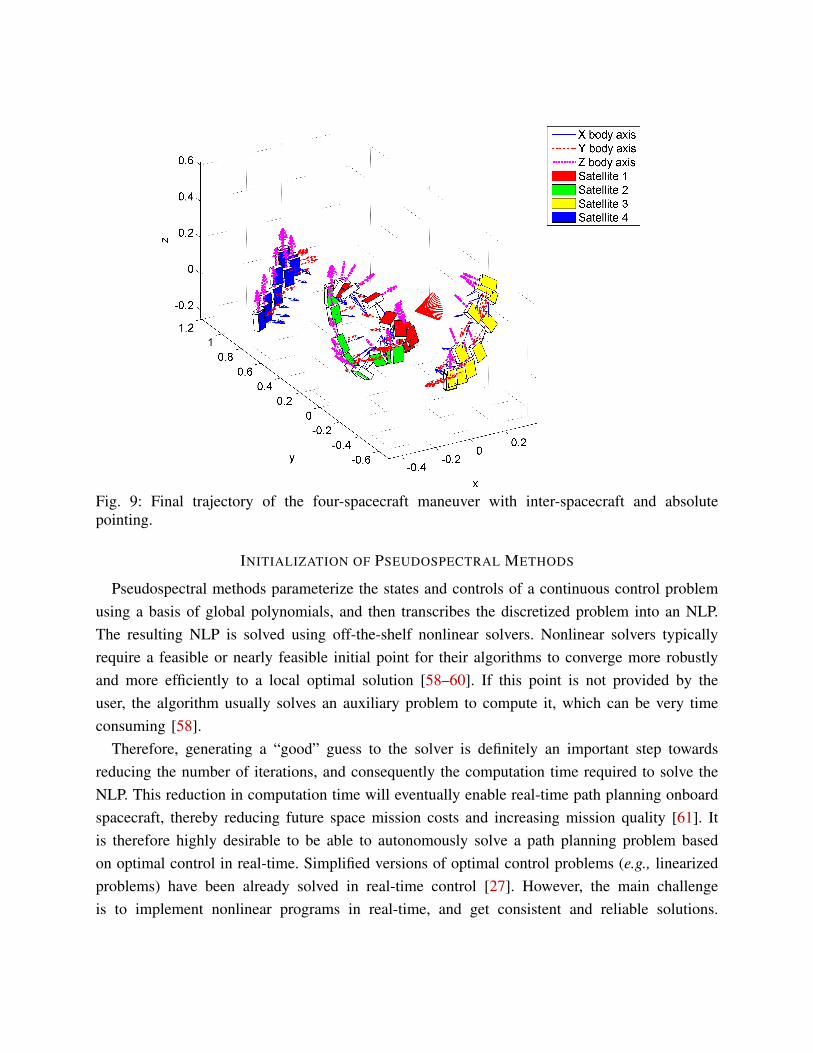
Fig. 9: Final trajectory of the four-spacecraft maneuver with inter-spacecraft and absolutepointing.

INITIALIZATION OF PSEUDOSPECTRAL METHODS

Pseudospectral methods parameterize the states and controls of a continuous control problemusing a basis of global polynomials, and then transcribes the discretized problem into an NLP.The resulting NLP is solved using off-the-shelf nonlinear solvers. Nonlinear solvers typicallyrequire a feasible or nearly feasible initial point for their algorithms to converge more robustlyand more efficiently to a local optimal solution [58–60]. If this point is not provided by theuser, the algorithm usually solves an auxiliary problem to compute it, which can be very timeconsuming [58].

Therefore, generating a “good” guess to the solver is definitely an important step towardsreducing the number of iterations, and consequently the computation time required to solve theNLP. This reduction in computation time will eventually enable real-time path planning onboardspacecraft, thereby reducing future space mission costs and increasing mission quality [61]. Itis therefore highly desirable to be able to autonomously solve a path planning problem basedon optimal control in real-time. Simplified versions of optimal control problems (e.g., linearizedproblems) have been already solved in real-time control [27]. However, the main challengeis to implement nonlinear programs in real-time, and get consistent and reliable solutions.

Pseudospectral methods have the potential to be solved in real-time because they provide highlyaccurate solutions even with a relatively small number of discretization nodes i.e., a smallerproblem size. Algorithms that can determine feasible initial guesses for pseudospectral methodswill help reduce the computation time of these methods, and therefore make them more suitablefor real-time applications.

Survey of Initialization Techniques

Note that generating a feasible initial guess for a highly constrained nonlinear problem can beas complicated as solving the nonlinear problem itself. Many researchers have suggested waysto compute acceptable initial guesses, with the general rule of thumb being that the closer theguess is to feasibility, the faster the solver should converge to the optimal solution. There havebeen different suggestions on how to generate a good guess to initialized a nonlinear solverwhen solving the transcribed optimal control problem:

1) One common way is that the user develops a good guess for the control using common-engineering-sense [62]. Then the states are computed by using numerical integration. Theguess (states and controls) will most likely not be feasible, in the sense that it will notsatisfy the boundary conditions. Then looking at the resulting guess and using knowledgeof the problem, the user can create a new guess for the control, and repeat the process, untilthe guess is good enough. But this method can be time consuming, and it is not guaranteedto converge to a feasible answer.

2) Another method is known as the mesh refinement technique [29]. The idea is to start witha coarse grid (i.e., low number of discretization nodes) and use any guess (e.g., randomlychosen) as an initial starting point for the nonlinear solver. Then, if necessary, refinethe discretization (i.e., increase the number of discretization nodes), and then repeat theoptimization steps using the output of the previous step as the initial guess of the currentstep. This process can be very time consuming, and therefore current approaches do notappear to be feasible for online planning of complex reconfiguration maneuvers consistingof several spacecraft [29, 58].

3) A third way of initializing the NLP is by using a “warm” start approach [49, 63]. A warmstart uses the output of a similar version of the NLP as the initial guess for the actualproblem. A similar version is either exactly the same problem run previously (i.e., offlinecompared to online), or a simplified version of the problem. Warm starts are widely usedfor active set solvers, but there are still many difficulties in applying them to interior pointmethods [64]. In addition, using a warm start technique based on an offline computationmight not suitable for online implementation where the environment is affected by dis-turbances, and where previous solutions might not be feasible. So warm start approaches

Continuous OptimalControl Problem

Feasible Initial Guessto Original Problem

RRTSolution

Simplified PathPlanning Problem

Discretize& Simplify

Solve usingRRT planner

Augment usingtransition step

Fig. 10: Steps Involved in Generating a Feasible Initial Guess to the Optimal Control Problem.This guess serves as a starting point to the NLP resulting from the transcription of the optimalcontrol problem using Pseudospectral methods.

should be chosen with care to minimize the inefficiency and inconsistency that they canintroduce.

4) A similar approach to warm starts is called homotopy methods that first solve a simplerversion of the problem and then continuously modify the solution towards the originallydesired problem statement. But homotopy methods require expensive computation and theirperformance depends on a successful selection of a homotopy which matches best thestructure of the problem [65].

The following briefly discusses the RRT-based warm start technique introduced earlier in thispaper and then illustrates the significant improvement it provided to the computation time of thepseudospectral method.

RRT Planner Initialization

The RRT-based initialization has been used in the first stage of the two-stage path planningalgorithm described earlier. It is illustrated in Figure 10. It is an efficient warm start approach thatinitializes the NLP resulting from the transcription of the continuous optimal control problem.This warm start is formulated as an RRT path planning problem, with no differential constraints.The output of the RRT planner is then augmented with feasible dynamics that are propagatedfrom source to destination using an algorithm that ensures feasibility at each node. This processof augmenting the output of the randomized planner is called the transition phase (see sectionThe Augmentation with Feasible Dynamics). The resulting output is a feasible initial guess tothe complete optimal control problem. The paper uses an improved version of the bidirectionalrapidly-exploring random trees (RRT) that is described in Ref. [22].

Illustration of the RRT improvement

This section illustrates the improvement that the RRT initialization step brings to optimalcontrol problems solved using pseudospectral methods. To do so, it revisits the multi-spacecraftreconfiguration maneuver problem with path constraints (see Equations (1) – (23)), but placesmore emphasis on the importance of the role of first step (the RRT initialization) on the solutionperformance of the optimal control problem formed in the second stage. This initialization

technique should be straightforward to adapt to several other optimal control problem examples.Recall that the optimal control problem of interest is transcribed into an NLP using the Gausspseudospectral method (GPM) which has shown promise both in the accuracy of the solutionand post-optimality analysis of optimal control problems [26].

To highlight the improvement of the RRT step, several reconfiguration maneuvers of increasingcomplexity are solved twice: 1) using the RRT step to find a feasible initial guess, and 2) using a“cold” start approach which relies on the nonlinear solver to find an initial guess. The examplesconsist of reconfiguration maneuvers that include stay outside constraints (e.g., sun avoidance),inter-spacecraft collision avoidance constraints, and obstacle avoidance constraints. These arehard non-convex constraints. But the examples do not include inter-spacecraft constraints suchas those described in Figure 1. Including the inter-spacecraft constraints resulted in the nonlinearsolver failing to converge when using the cold approach. Thus the RRT initial guess is essentialin those cases. Recall that inter-spacecraft constraints are coupling constraints i.e., they affect, ina coupled way, the position and attitudes of the spacecraft. Therefore the feasible set of problemshaving coupled constraints is usually a very small region, which explains the difficulties of thenonlinear solver. The examples below are solved using GPOCS [56]. Both optimality and feasi-bility tolerances are set to 10−4. It was observed by numerical experimentation that decreasingthese tolerances further achieve marginal improvement while significantly increasing computationtime [44]. The computation times and costs of the following examples are summarized in Table Iand Table II.

Single Spacecraft Maneuver: This example is a simple translation from the position [0, 0, 0]T

to [1, 1, 1]T with a 180◦ rotation around the Z axis. The spacecraft has to avoid pointing its Xaxis in the sun direction, which is represented by the vector [ 1√

2, 1√

2, 0]T , surrounded by a cone

of 30◦ half angle. It also has to avoid colliding with a fixed obstacle centered at [0.6, 0.5, 0.5]T ,with radius equal to 0.15 m.

Diagonally Crossing Maneuver: This problem consists of a three-spacecraft maneuver. Space-craft 1 and 2 start at [0, 0, 0]T and [1, 1, 1]T , the opposite corners of a cube of side 1. They mustswitch position and make a 90◦ rotation around the inertial Z axis. A third spacecraft, spacecraft3 starts at [1, 0, 0]T and ends at [0, 1, 1]T . It also performs at 90◦ rotation. The maneuver ofspacecraft three crosses diagonally those of the other two spacecraft. All three spacecraft have toavoid a fixed obstacle located at [0.3, 0.3, 0.3]T with radius equal to 0.2 m. They also must avoidpointing their body X axis in the sun direction, which is represented by the vector [ 1√

2, 1√

2, 0]T ,

surrounded by a cone of 30◦ half angle. Figure 11 shows the RRT initial guess, the final trajectoryof the problem that uses the RRT guess, and the final trajectory that uses the cold start approach.Two circles surrounding the spacecraft help visualize the actual boundaries of the spacecraft.

a. RRT Initial Guess

b. Final trajectory solved using RRT initial guess.

c. Final trajectory solved with a cold start approach.

Fig. 11: RRT Path and Final Trajectories for the Three-Spacecraft Example

TABLE I: Comparison of computation times of reconfiguration maneuvers for formation ofincreasing size solved using a Gauss pseudospectral method (average over 10 runs)

Time (s)Example w/o RRT with RRT Time Ratio

1 s/c 35 24 1.462 s/c 103 67 1.543 s/c 335 171 1.964 s/c 478 228 2.105 s/c 834 356 2.34

Formation Reflection with Four Spacecraft: This example consists of four spacecraft that startin a square formation, and end in another reflected square formation. Spacecraft 1 and spacecraft3 start at [0, 1, 0]T and [2, 1, 0]T , respectively. They must end at their original positions. Theymust also rotate 90◦ around the inertial Z axis. Spacecraft 2 and 4 start at [1, 0, 0]T and [1, 2, 0]T ,and must switch their position. They must also rotate 180◦ around the inertial Z axis. Allspacecraft must avoid pointing their X body axis inside two cones of 50◦ along the X and -Xinertial directions. They must also avoid colliding with a fixed obstacle located at the center ofthe square, with radius equal to 0.25 m. The pointing constraints lead to a non-trivial rotationmaneuvers for both spacecraft 1 and 3. The fixed obstacle makes the trajectories of spacecraft 2and 4 a more challenging one. In Summary, the maneuver is a reflection of a square formationaround a line passing through the fixed positions of Spacecraft 1 and 3.

Formation Rotation with Five Spacecraft: This example consists of five spacecraft starting ina pyramid formation. Spacecraft 5 starts at the apex of the pyramid, while spacecraft 1 through 4form its square base. Each spacecraft must move to the next spacecraft position in the sequence(spacecraft 2 moves to the spacecraft 1 position, 3 to 2, 4 to 3, 5 to 4, and 1 to 5). Each spacecraftmust also end the maneuver pointing in the direction where the next spacecraft in the sequencewas pointing at the beginning of the maneuver. Thus, the final configuration is a rotated versionof the original pyramid formation. The spacecraft must avoid pointing their X body axis towardsthe sun direction represented by the vector [ 1√

2, 1√

2, 0]T , surrounded by a cone of 20◦ half angle.

They must also avoid colliding with two fixed obstacles of radius equal to 0.15 m. Figure 12shows the RRT initial guess, the final trajectory of the problem that uses the RRT guess, andthe final trajectory that uses the cold start approach.

Performance Comparison

Table I summarizes the computation times of the examples used to show the improvement ofthe RRT initialization on problems solved using pseudospectral methods. The with RRT timeincludes the time of the RRT step, the transition step, and the time required by the GPOCS

a. RRT Initial Guess

b. Final trajectory solved using RRT initial guess.

c. Final trajectory solved with a cold start approach.

Fig. 12: RRT Path and Final Trajectories for the Five-Spacecraft Example

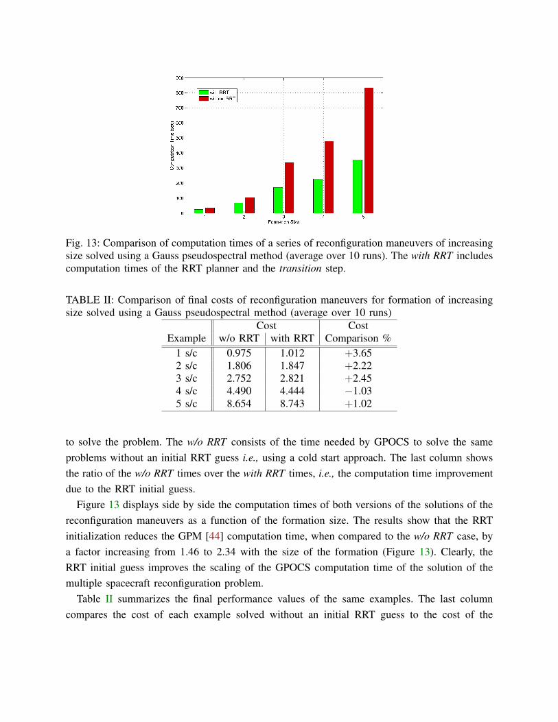
Fig. 13: Comparison of computation times of a series of reconfiguration maneuvers of increasingsize solved using a Gauss pseudospectral method (average over 10 runs). The with RRT includescomputation times of the RRT planner and the transition step.

TABLE II: Comparison of final costs of reconfiguration maneuvers for formation of increasingsize solved using a Gauss pseudospectral method (average over 10 runs)

Cost CostExample w/o RRT with RRT Comparison %

1 s/c 0.975 1.012 +3.652 s/c 1.806 1.847 +2.223 s/c 2.752 2.821 +2.454 s/c 4.490 4.444 −1.035 s/c 8.654 8.743 +1.02

to solve the problem. The w/o RRT consists of the time needed by GPOCS to solve the sameproblems without an initial RRT guess i.e., using a cold start approach. The last column showsthe ratio of the w/o RRT times over the with RRT times, i.e., the computation time improvementdue to the RRT initial guess.

Figure 13 displays side by side the computation times of both versions of the solutions of thereconfiguration maneuvers as a function of the formation size. The results show that the RRTinitialization reduces the GPM [44] computation time, when compared to the w/o RRT case, bya factor increasing from 1.46 to 2.34 with the size of the formation (Figure 13). Clearly, theRRT initial guess improves the scaling of the GPOCS computation time of the solution of themultiple spacecraft reconfiguration problem.

Table II summarizes the final performance values of the same examples. The last columncompares the cost of each example solved without an initial RRT guess to the cost of the

same example solved with an RRT initial guess. A positive value indicates the percentage ofimprovement (i.e., decrease) in the cost of the w/o RRT case when compared to the with RRTone. Similarly, a negative value indicates the percentage of degradation (i.e., increase) in thecost. The results show that the cost values are very comparable. In the worst case, the cost ofw/o RRT version is 3.65% better. For the largest formation, the five spacecraft reconfigurationshown in Figure 12, the w/o RRT cost is only 1.02% better.

Finally, it should be emphasized that, when the cold approach is adopted, GPOCS fails (after10 attempts) to solve examples that include inter-spacecraft pointing constraints. Such examplesare described in the illustration of the two-stage approach earlier in this paper. Recall that theseconstraints tightly couple the position and attitude of the spacecraft. Thus, they significantlyincrease the complexity of the problem to be solved by the nonlinear solver that GPOCS relies onin its solution process. However, when provided with an RRT guess, GPOCS is able to convergeto a solution. So not only does the RRT guess reduce the computation times of the reconfigurationmaneuver problem, it also enables the solution of a complex class of reconfiguration problemsthat include inter-spacecraft constraints.

CONCLUSIONS

This paper presented a two-stage path planning technique for designing multiple spacecraftreconfiguration maneuvers with various path constraints. The main idea was to combine animproved RRT planner with a Gauss pseudospectral method to obtain highly accurate solutionswith reduced computation times that could enable an online implementation. Several complexexamples demonstrated the validity of this approach, and it has been used to design reconfig-uration maneuvers that were successfully performed on SPHERES micro-satellites onboard theInternational Space Station [55]. This paper also showed the importance of an initialization stepbased on an RRT planner to the solution of optimal control problems solved using pseudospectralmethods. It showed that this step 1) reduced the computation time of the solutions by up to afactor of 2.34 for a five-spacecraft reconfiguration maneuver, and 2) made it possible to solvea more complex class of such problems that include highly coupled inter-spacecraft pointingconstraints.

ACKNOWLEDGMENTS

This research was funded in part by the Payload Systems Inc. SPHERES Autonomy andIdentification Testbed Grant #012650-001 (PI: Professor David Miller, director of the SpaceSystems Laboratory at MIT), NASA Grants #NAG3-2839 and #NAG5-10440, and Le FondsQuebecois de la Recherche sur la Nature et les Technologies (FQRNT) Graduate Award. The

authors would like to thank Professor Anil Rao and Dr. Geoffrey Huntington for their technicalassistance with the GPOCS software.

REFERENCES

[1] C. Sultan, S. Seereram, and R. K. Mehra, “Deep Space Formation Flying Spacecraft PathPlanning,” The International Journal of Robotics Research, vol. 26, no. 4, pp. 405–430,2007.

[2] P. R. Lawson, “The Terrestrial Planet Finder,” in Proceedings of the IEEE AerospaceConference, vol. 4, March 2001, pp. 2005–2011.

[3] “NASA Laser Interferometer Space Antenna Website.” [Online]. Available: http://lisa.nasa.gov/

[4] C. V. M. Fridlund, “Darwin: The Infrared Space Interferometer Darwin and Astronomy,”ESA, Tech. Rep. SP-451, 2000.

[5] A. Das and R. Cobb, “TechSat21Space Missions Using Collaborating Constellations ofSatellites,” in 12th Annual Small Satellite Conference, no. Paper SSC98-VI-1. Reston,VA: AIAA, August 1998.

[6] “Broad Agency Announcement (BAA07-31) System F6 for Defense Advanced ResearchProjects Agency (DARPA),” 2007. [Online]. Available: http://www.darpa.mil/ucar/solicit/baa07-31/f6 baa final 07-16-07.doc

[7] A. Robertson, G. Inalhan, and J. How, “Spacecraft Formation Flying Control Design forthe Orion Mission,” in In Proceedings of the AIAA Conference on Navigation, Portland,OR, 1999.

[8] F. H. Bauer, J. O. Bristow, J. R. Carpenter, J. L. Garrison, K. Hartman, T. Lee, A. Long,D. Kelbel, V. Lu, J. P. How, F. Busse, P. Axelrad, , and M. Moreau, “Enabling SpacecraftFormation Flying through Spaceborne GPS and Enhanced Autonomy Technologies,” SpaceTechnology, vol. 20, pp. 175–185, 2001.

[9] D. P. Scharf, F. Y. Hadaegh, and S. R. Ploen, “A Survey of Spacecraft FormationFlying Guidance and Control. Part II: Control,” in Proceedings of the American ControlConference, vol. 4, 30 June-2 July 2004, pp. 2976–2985.

[10] ——, “A Survey of Spacecraft Formation Flying Guidance and Control. Part I: Guidance,”in Proceedings of American Control Conference, vol. 2, Jun 2003, pp. 1733–1739.

[11] I. M. Garcia, “Nonlinear Trajectory Optimization with Path Constraints Applied to Space-craft Reconfiguration Maneuvers,” Master’s thesis, Massachussets Institute of Technology,2005.

[12] A. Richards, T. Schouwenaars, J. P. How, and E. Feron, “Spacecraft Trajectory Planningwith Avoidance Constraints,” Journal of Guidance control and dynamics, vol. 25, no. 4,pp. 755–764, 2002.

[13] R. K. Prasanth, J. D. Boskovic, and R. K. Mehra, “Mixed integer/LMI programs for low-level path planning,” in Proceedings of the American Control Conference, vol. 1, 2002, pp.608–613 vol.1.

[14] F. McQuade, R. Ward, and C. McInnes, “The Autonomous Configuration of Satellite For-mations using Generic Potential Functions,” in Proceedings of the International SymposiumFormation Flying, 2002.

[15] R. O. Saber, W. B. Dunbar, and R. M. Murray, “Cooperative Control of Multi-VehicleSystems using Cost Graphs and Optimization,” in Proceedings of the American ControlConference, vol. 3, 2003, pp. 2217–2222.

[16] E. Frazzoli, M. A. Dahleh, E. Feron, and R. P. Kornfeld, “A Randomized Attitude SlewPlanning Algorithm for Autonomous Spacecraft,” AIAA Guidance, Navigation, and ControlConference and Exhibit, Montreal, Canada, 2001.

[17] L. E. Kavraki, P. Svestka, C. L. J, and M. H. Overmars, “Probabilistic Roadmaps for PathPlanning in High-Dimensional Configuration Spaces,” IEEE Transactions on Robotics andAutomation, vol. 12, no. 4, pp. 566–580, 1996.

[18] L. E. Kavraki, M. N. Kolountzakis, and J. C. Latombe, “Analysis of probabilistic roadmapsfor path planning,” in IEEE International Conference on Robotics and Automation, vol. 4,1996, pp. 3020–3025 vol.4.

[19] J. M. Phillips, L. E. Kavraki, and N. Bedrosian, “Spacecraft Rendezvous and DockingWith Real-Time Randomized Optimization,” in AIAA Guidance, Navigation and ControlConference, Austin, TX, August 2003.

[20] E. Frazzoli, “Quasi-Random Algorithms for Real-Time Spacecraft Motion Planning andCoordination,” Acta Astronautica, vol. 53, no. 4-10, pp. 485–495, 2003.

[21] I. Garcia and J. P. How, “Trajectory Optimization for Satellite Reconfiguration ManeuversWith Position and Attitude Constraints,” in American Control Conference, 2005. Proceed-ings of the 2005, vol. 2, 2005, pp. 889–894.

[22] ——, “Improving the Efficiency of Rapidly-exploring Random Trees Using a PotentialFunction Planner,” in IEEE Conference on Decision and European Control Conference,2005, pp. 7965–7970.

[23] I. Ross and C. D’Souza, “Rapid Trajectory Optimization of Multi-Agent Hybrid Systems,”in AIAA Guidance, Navigation, and Control Conference and Exhibit, 2004.

[24] G. T. Huntington and A. V. Rao, “Optimal Configuration Of Spacecraft Formations Via AGauss Pseudospectral Method,” Advances in the Astronautical Sciences, Part I, vol. 120,pp. 33–50, 2005.

[25] Q. Gong, W. Kang, and I. M. Ross, “A Pseudospectral Method for the Optimal Controlof Constrained Feedback Linearizable Systems,” in Proceedings of Conference on ControlApplications on, 2005, pp. 1033–1038.

[26] G. T. Huntington and A. V. Rao, “Optimal Reconfiguration Of A Tetrahedral FormationVia A Gauss Pseudospectral Method,” Advances in the Astronautical Sciences, Part II, vol.123, pp. 1337–1358, 2006.

[27] G. T. Huntington, “Advancement and Analysis of a Gauss Pseudospectral Transcriptionfor Optimal Control Problems,” Ph.D. dissertation, Massachusetts Institute of Technology,June 2007.

[28] J. H. Reif, “Complexity of the Mover’s Problem and Generalizations,” in IEEE Symposiumon Foundations of Computer Science, 1979, pp. 421–427.

[29] J. T. Betts and W. P. Huffman, “Mesh Refinement in Direct Transcription Methods forOptimal Control,” Optimal Control Applications and Methods, vol. 19, no. 1, pp. 1–21,1998.

[30] S. LaValle, “Rapidly-Exploring Random Trees: A New Tool for Path Planning. TechnicalReport 98-11, Computer Science Dept., Iowa State University,” Oct 1998.

[31] S. M. LaValle and J. J. J. Kuffner, “Randomized kinodynamic planning,” in Robotics andAutomation, 1999. Proceedings. 1999 IEEE International Conference on, vol. 1, 1999, pp.473–479.

[32] D. A. Benson, G. T. Huntington, T. P. Thorvaldsen, and A. V. Rao, “Direct TrajectoryOptimization and Costate Estimation via an Orthogonal Collocation Method,” Journal ofGuidance, Control, and Dynamics, vol. 29, no. 6, pp. 1435–1440, November-December2006.

[33] B. R. Donald, P. G. X. J. F. Canny, and J. H. Reif, “Kinodynamic Motion Planning,” Journalof the ACM, vol. 40, no. 5, pp. 1048–1066, 1993.

[34] J. J. Kuffner, “Motion Planning with Dynamics,” Physiqual, March 1998.[35] D. Hsu, R. Kindel, J. Latombe, and S. Rock, “Randomized Kinodynamic Motion Planning

with Moving Obstacles,” Int. J. Robotics Research, vol. 21, no. 3, pp. 233–255, 2002.[36] E. Frazzoli, M. A. Dahleh, and E. Feron, “Real-time Motion Planning for Agile Autonomous

Vehicles,” in American Control Conference, vol. 1, 2001, pp. 43–49.[37] I. Belousov, C. Esteves, J. P. Laumond, and E. Ferre, “Motion Planning for the Large Space

Manipulators with Complicated Dynamics,” in International Conference on IntelligentRobots and Systems, IEEE/RSJ, 2005, pp. 2160–2166.

[38] S. M. Lavalle, Planning Algorithms. Cambridge University Press, 2006.[39] J. T. Betts, “Survey of Numerical Methods for Trajectory Optimization,” Journal of

Guidance, Control, and Dynamics, vol. 21, no. 2, pp. 193–207, 1998.[40] G. Elnagar, M. A. Kazemi, and M. Razzaghi, “The pseudospectral Legendre Method for

Discretizing Optimal Control Problems,” IEEE Transactions on Automatic Control, vol. 40,no. 10, pp. 1793–1796, 1995.

[41] G. N. Elnagar and M. A. Kazemi, “Pseudospectral Chebyshev Optimal Control ofConstrained Nonlinear Dynamical Systems,” Comput. Optim. Appl., vol. 11, no. 2, pp.195–217, 1998.

[42] I. M. Ross and F. Fahroo, “Convergence of Pseudospectral Discretizations of OptimalControl Problems,” in Proceedings of the 40th IEEE Conference on Decision and Control,vol. 4, 2001, pp. 3175–3177.

[43] M. D. Shuster, “Survey of Attitude Representations,” Journal of the Astronautical Sciences,vol. 41, pp. 439–517, Oct. 1993.

[44] G. S. Aoude, “Two-Stage Path Planning Approach for Designing Multiple SpacecraftReconfiguration Maneuvers and Application to SPHERES onboard ISS,” Master’sthesis, Massachusetts Institute of Technology, September 2007. [Online]. Available:http://dspace.mit.edu/bitstream/handle/1721.1/42050/230816006.pdf?sequence=1

[45] D. P. Scharf, F. Y. Hadaegh, and B. H. Kang, “On the validity of the double integratorapproximation in deep space formation flying,” in International Symposium FormationFlying Missions & Technologies, Toulouse, France, October 2002.

[46] A. G. Richards, “Trajectory Optimization using Mixed-Integer Linear Programming,”Master’s thesis, Massachusetts Institute of Technology, June 2002.

[47] Y. Kim, M. Mesbah, and F. Y. Hadaegh, “Dual-spacecraft formation flying in deep space- Optimal collision-free reconfigurations,” Journal of Guidance, Control, and Dynamics,vol. 26, no. 2, pp. 375–379, March 2003.

[48] A. Rahmani, M. Mesbahi, and F. Y. Hadaegh, “On the Optimal Balanced-Energy Formation

Flying Maneuvers,” 2005 AIAA Guidance, Navigation, and Control Conference and Exhibit;San Francisco, CA; USA; 15-18 Aug. 2005, pp. 1–8, 2005.

[49] P. E. Gill, W. Murray, and M. A. Saunders, “User’s Guide For SNOPT 5.3: A FortranPackage For Large-Scale Nonlinear Programming,” 1999.

[50] L. N. Trefethen, Spectral Methods in Matlab. Philadelphia: SIAM Press, 2000.[51] D. Benson, “A Gauss Pseudospectreal Transcription for Optimal Control,” Ph.D. disserta-

tion, Massachusetts Institute of Technology, 2005.[52] D. E. Kirk, Optimal Control Theory: An Introduction. Dover Publications, 1970.[53] A. S. Otero, A. Chen, D. W. Miller, and M. Hilstad, “SPHERES: Development of an ISS

Laboratory for Formation Flight and Docking Research,” in IEEE Aerospace ConferenceProceedings, vol. 1, 2002, pp. 59–73.

[54] J. Enright, M. Hilstad, A. Saenz-Otero, and D. Miller, “The SPHERES Guest ScientistProgram: Collaborative Science on the ISS,” in Proceedings of the IEEE AerospaceConference, vol. 1, 2004.

[55] G. S. Aoude, J. P. How, and D. W. Miller, “Reconfiguration Maneuver Experiments usingthe SPHERES tesbed onboard the ISS,” in 3rd International Symposium on FormationFlying, Missions and Technologies. Noordwijk, The Netherlands: ESA/ESTEC, April2008.

[56] A. V. Rao, User’s Manual for GPOCS Version 1.1: A MATLAB Implementation of theGauss Pseudospectral Method for Solving Non-Sequential Multiple-Phase Optimal ControlProblems, report 1 beta ed., May 2007.

[57] D. Hsu, L. Kavraki, J. Latombe, R. Motwani, and S. Sorkin, “On finding narrowpassages with probabilistic roadmap planners,” in Proceedings of the third workshop onthe algorithmic foundations of robotics on Robotics, Houston, TX, 1998, pp. 141–153.

[58] J. T. Betts, Practical methods for optimal control using nonlinear programming, ser.Advances in Design and Control. Philadelphia, PA: Society for Industrial and AppliedMathematics (SIAM), 2001, vol. 3.

[59] J. W. Chinneck, “The constraint consensus method for finding approximately feasible pointsin nonlinear programs,” INFORMS Journal on Computing, vol. 16, no. 3, pp. 255–265,2004.

[60] O. A. Elwakeil and J. S. Arora, “Methods for finding feasible points in constrainedoptimization,” AIAA journal, vol. 33, no. 9, pp. 1715–1719, 1995.

[61] N. Muscettola, B. Smith, S. Chien, C. Fry, G. Rabideau, K. Rajan, and D. Yan, “On-board Planning for Autonomous Spacecraft,” in In Proceedings of the Fourth InternationalSymposium on Artificial Intelligence, Robotics, and Automation for Space (iSAIRAS), July1997.

[62] I. M. Ross, User’s Manual for DIDO: A MATLAB Application Package for Solving OptimalControl Problems, Monterey, California, February 2004.

[63] J. Mitchell and B. Borchers, “Solving Real-World Linear Ordering Problems Using aPrimal-Dual Interior Point Cutting Plane Method,” Annals of Operations Research, vol. 62,no. 1, pp. 253–276, Dec. 1996.

[64] R. A. Bartlett, A. Wachter, and L. T. Biegler, “Active Set vs. Interior Point Strategies forModel Predictive Control,” in Proceedings of the American Control Conference, vol. 6,2000, pp. 4229–4233.

[65] K. Reif, K. Weinzierl, A. Zell, and R. Unbehauen, “Application of homotopy methods tononlinear control problems,” Decision and Control, 1996., Proceedings of the 35th IEEE,vol. 1, pp. 533–538 vol.1, 11-13 Dec 1996.