two-stage stochastic optimization. an application in the
TRANSCRIPT
Two-Stage Stochastic Optimization.An Application in the Third Sector
Final Degree DissertationDegree in Mathematics
Sara Laconcepcion Moraza
Supervisor:
Marıa Merino Maestre
Leioa, 24th February 2015

This work is licensed under the Creative Commons Atribution 4.0 international license

Contents
List of Figures I
List of Tables III
Acknowledgements V
Abstract VII
1 Introduction 1
1.1 Social and Mathematical Motivation . . . . . . . . . . . . . . . . . . . . . . . . . 1
1.2 Aims of the project . . . . . . . . . . . . . . . . . . . . . . . . . . . . . . . . . . . 2
1.3 Scientific literature . . . . . . . . . . . . . . . . . . . . . . . . . . . . . . . . . . . 3
1.4 Organization of the project . . . . . . . . . . . . . . . . . . . . . . . . . . . . . . 4
2 Optimization Models under Uncertainty 5
2.1 Deterministic Linear Programming . . . . . . . . . . . . . . . . . . . . . . . . . . 5
2.2 Stochastic Linear Programming . . . . . . . . . . . . . . . . . . . . . . . . . . . . 7
2.2.1 Probability Spaces and Random Variables . . . . . . . . . . . . . . . . . . 8
2.2.2 Decisions and recourses . . . . . . . . . . . . . . . . . . . . . . . . . . . . 10
2.2.3 Non-anticipativity principle . . . . . . . . . . . . . . . . . . . . . . . . . . 12
2.2.4 Two-Stage Model in Compact Representation . . . . . . . . . . . . . . . . 12
2.2.5 Two-Stage Model in Splitting Variable Representation . . . . . . . . . . . 15
2.2.6 Some two-stage examples . . . . . . . . . . . . . . . . . . . . . . . . . . . 17
3 The Value of Perfect Information and the Stochastic Solution 21
3.1 Wait-and-See solution (WS) . . . . . . . . . . . . . . . . . . . . . . . . . . . . . . 22
3.2 Expected Value problem (EV) . . . . . . . . . . . . . . . . . . . . . . . . . . . . . 25
3.3 Expected result of using the EV solution (EEV) . . . . . . . . . . . . . . . . . . 27
3.4 The Expected Value of Perfect Information (EVPI) . . . . . . . . . . . . . . . . . 31
3.5 The Value of Stochastic Solutions (VSS) . . . . . . . . . . . . . . . . . . . . . . . 31
3.6 Main Inequalities . . . . . . . . . . . . . . . . . . . . . . . . . . . . . . . . . . . . 32
3.7 The Relationship between EVPI and VSS . . . . . . . . . . . . . . . . . . . . . . 34
4 An Application in the Third Sector: Hazia Project 394.1 Background . . . . . . . . . . . . . . . . . . . . . . . . . . . . . . . . . . . . . . . 394.2 Diet stochastic models and alternative models . . . . . . . . . . . . . . . . . . . . 404.3 Dataset . . . . . . . . . . . . . . . . . . . . . . . . . . . . . . . . . . . . . . . . . 43
4.3.1 First stage prices and nutrients . . . . . . . . . . . . . . . . . . . . . . . . 434.3.2 Second stage prices and nutrients . . . . . . . . . . . . . . . . . . . . . . . 444.3.3 Nutricional bounds . . . . . . . . . . . . . . . . . . . . . . . . . . . . . . . 454.3.4 Data preliminar analysis . . . . . . . . . . . . . . . . . . . . . . . . . . . . 47
4.4 Analysis and Results . . . . . . . . . . . . . . . . . . . . . . . . . . . . . . . . . . 504.4.1 Solutions for Model 1.a. . . . . . . . . . . . . . . . . . . . . . . . . . . . . 504.4.2 Solutions for Model 2.a. . . . . . . . . . . . . . . . . . . . . . . . . . . . . 534.4.3 Solutions for Model 1.b. . . . . . . . . . . . . . . . . . . . . . . . . . . . . 554.4.4 Solutions for Model 2.b. . . . . . . . . . . . . . . . . . . . . . . . . . . . . 56
4.5 Conclusions and suggestions . . . . . . . . . . . . . . . . . . . . . . . . . . . . . . 58
5 Conclusions 59
A GAMS CODE: Examples 61
B GAMS CODE: Application in the third sector 63
References 65
List of Figures
2.1 Example of a scenario tree . . . . . . . . . . . . . . . . . . . . . . . . . . . . . . . 92.2 Non-ancitipativity principle . . . . . . . . . . . . . . . . . . . . . . . . . . . . . . 122.3 Scenario tree in compact representation . . . . . . . . . . . . . . . . . . . . . . . . . . . 142.4 Matrix structure in compact representation . . . . . . . . . . . . . . . . . . . . . . . . . 142.5 Scenario tree in splitting variable representation . . . . . . . . . . . . . . . . . . . 152.6 Matrix structure in splitting variable representation . . . . . . . . . . . . . . . . 162.7 Matrix structure under one scenario ω . . . . . . . . . . . . . . . . . . . . . . . . 162.8 Scenario tree for Case 1 and Case 2 . . . . . . . . . . . . . . . . . . . . . . . . . . 172.9 Scenario tree for Case 3 . . . . . . . . . . . . . . . . . . . . . . . . . . . . . . . . 20
4.1 Pie chart of users for age range . . . . . . . . . . . . . . . . . . . . . . . . . . . . . . 464.2 Pie chart for families . . . . . . . . . . . . . . . . . . . . . . . . . . . . . . . . . . 474.3 Pie chart for users . . . . . . . . . . . . . . . . . . . . . . . . . . . . . . . . . . . 474.4 Energy, macronutrients and mineral % satisfaction depending on the set . . . . . 494.5 Optimal WS, SP and EEV solutions for |Ω| = 24 scenarios . . . . . . . . . . . . . 514.6 Histogram of ZWS for Model 1.a. . . . . . . . . . . . . . . . . . . . . . . . . . . . 524.7 Histogram of ZSP for Model 1.a. . . . . . . . . . . . . . . . . . . . . . . . . . . . 524.8 Comparison of nutrients requirement satisfaction for Model 2.a. . . . . . . . . . . 544.9 Comparison of percentages of nutrients satisfied for Model 2.b. . . . . . . . . . . 57
I

II

List of Tables
2.1 Cost and nutrients per aliment . . . . . . . . . . . . . . . . . . . . . . . . . . . . 6
2.2 Nutrient requirements per day and person . . . . . . . . . . . . . . . . . . . . . . 6
2.3 Price of each product depending on the market . . . . . . . . . . . . . . . . . . . 17
2.4 Optimal SP solution for Case 1 . . . . . . . . . . . . . . . . . . . . . . . . . . . . 18
2.5 Nutrients of each product depending on the market . . . . . . . . . . . . . . . . . 18
2.6 Optimal SP solution for Case 2 . . . . . . . . . . . . . . . . . . . . . . . . . . . . 19
2.7 Bounds according to each nutrient and scenario . . . . . . . . . . . . . . . . . . . 19
2.8 Optimal SP solution for Case 3 . . . . . . . . . . . . . . . . . . . . . . . . . . . . 20
3.1 Optimal WS solutions for Case 1 . . . . . . . . . . . . . . . . . . . . . . . . . . . 23
3.2 Optimal WS solutions of Case 2 . . . . . . . . . . . . . . . . . . . . . . . . . . . . 24
3.3 Optimal WS solutions of Case 3 . . . . . . . . . . . . . . . . . . . . . . . . . . . . 24
3.4 Optimal EEV solutions for Case 1 . . . . . . . . . . . . . . . . . . . . . . . . . . 28
3.5 Optimal EEV solutions for Case 2 . . . . . . . . . . . . . . . . . . . . . . . . . . 29
3.6 Optimal EEV solutions for Case 3 . . . . . . . . . . . . . . . . . . . . . . . . . . 30
3.7 EVPI solutions for Cases 1, 2 and 3 . . . . . . . . . . . . . . . . . . . . . . . . . 31
3.8 VSS solutions for Cases 1, 2 and 3 . . . . . . . . . . . . . . . . . . . . . . . . . . 32
3.9 Proposition 3.1 verified for Cases 1, 2 and 3 . . . . . . . . . . . . . . . . . . . . . 32
3.10 Proposition 3.2 verified for Cases 1, 2 and 3 . . . . . . . . . . . . . . . . . . . . . 33
3.11 Proposition 3.4 verified for Cases 1, 2 and 3 . . . . . . . . . . . . . . . . . . . . . 34
4.1 Energy, macronutrients and minerals of each product by BEDCA . . . . . . . . . 43
4.2 Energy, macronutrients and minerals of each product taken from the Food Bank 44
4.3 Selection of the most different products . . . . . . . . . . . . . . . . . . . . . . . 45
4.4 Energy estimation . . . . . . . . . . . . . . . . . . . . . . . . . . . . . . . . . . . . 46
4.5 Energy, macronutrients and mineral requirement bounds . . . . . . . . . . . . . . 46
4.6 Monthly users distribution . . . . . . . . . . . . . . . . . . . . . . . . . . . . . . . 47
4.7 Monthly set of products for sets of np users . . . . . . . . . . . . . . . . . . . . . 48
4.8 Nutrients satisfied per person and day . . . . . . . . . . . . . . . . . . . . . . . . 48
4.9 Satisfied energy, macronutrients and mineral . . . . . . . . . . . . . . . . . . . . . 49
4.10 Comparison of values EV, WS, SP, EEV, EVPI and VSS for Model 1.a. . . . . . 50
4.11 Total decisions for Model 1.a. . . . . . . . . . . . . . . . . . . . . . . . . . . . . . 52
4.12 Monthly set of products for np people for Model 1.a. . . . . . . . . . . . . . . . . 53
4.13 Comparison of values EV, WS, SP, EEV, EVPI and VSS for Model 2.a. . . . . . 53
III

4.14 Total decisions for Model 2.a. . . . . . . . . . . . . . . . . . . . . . . . . . . . . . 544.15 Monthly set of products for np people for Model 2.a. . . . . . . . . . . . . . . . . 544.16 Comparison of values EV, WS, SP, EEV, EVPI and VSS for Model 1.b. . . . . . 554.17 Best and worst cases depending on the problem for Model 1.b. . . . . . . . . . . 554.18 Monthly set of products for np people for Model 1.b. . . . . . . . . . . . . . . . . 564.19 Comparison of values EV, WS, SP, EEV, EVPI and VSS for Model 2.b. . . . . . 564.20 Best and worst cases depending on the problem for Model 2.b. . . . . . . . . . . 564.21 Monthly set of products for np people for Model 2.b. . . . . . . . . . . . . . . . . 574.22 Nutritional satisfaction and budget of generated models . . . . . . . . . . . . . . 58
IV

Acknowledgements
Quiero expresar mi agradecimiento a mis padres y a mi hermana, por animarme y apoyarmesiempre en todas las decisiones que he tomado. A Ainara, por estar siempre que lo he necesitado,por su apoyo en los momentos mas duros y por no dejar que me rinda.
A mi tutora Marıa Merino Maestre, por su ayuda y dedicacion; por haberme dado la opor-tunidad y haber aceptado dirigirme en este Trabajo de Fin de Grado.
Al profesor Fernando Tusell Palmer del departamento de Economıa Aplicada III (Econometrıay Estadıstica) de la Facultad de Ciencias Economicas y Empresariales, por facilitarnos el accesoal servidor u107499 del Laboratorio de Economıa Cuantitativa (LEC) para poder llevar a cabola experiencia computacional de la aplicacion nutricional de este trabajo.
A Paola Dapena Montes, responsable del proyecto Hazia en la asociacion sin animo de lucroSortarazi, por facilitar el acceso al almacen de alimentos y la consulta de informacion sobre lasbases de datos de las familias usuarias del servicio.
A la profesora Ana Marıa Rocandio de Pablo, del area de Nutricion y Bromatologıa, deldepartamento de Farmacia y Ciencias de los Alimentos, de la Facultad de Farmacia, por suasesoramiento en los aspectos nutricionales necesarios para realizar este trabajo.
A la profesora Leire Escajedo San Epifanio, investigadora principal del proyecto Universidad-Sociedad US 14/19 ”Urban Elika - Elikagaiak denontzat”, por su invitacion al Congreso Interna-cional Multidisciplinar ”Envisioning a Future without Food Waste and Food Poverty: SocietalChallenges”, celebrado en noviembre de 2015.
A Marıa del Mar Lledo Sainz de Rozas (subdirectora de Calidad e Innovacion) y Amaia InzaBartolome, de la Facultad de Relaciones Laborales y Trabajo Social, por facilitar el acceso amaterial bibliografico sobre la aplicacion de interes social.
A todo el equipo del proyecto de Innovacion Educativa HBP-PIE 2014-16 ”CTs de Compro-miso Etico y Social. Las competencias Transversales de Compromiso Etico y Social en TFG deResponsabilidad Social contra la Pobreza Alimentaria en la CAPV”, por el apoyo prestado enla realizacion de este Trabajo Fin de Grado.
V

VI
Laburpena
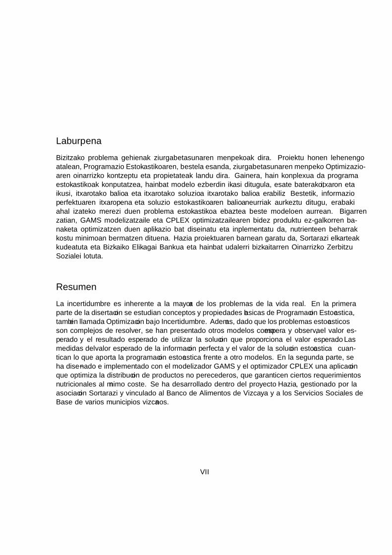
Bizitzako problema gehienak ziurgabetasunaren menpekoak dira. Proiektu honen lehenengoatalean, Programazio Estokastikoaren, bestela esanda, ziurgabetasunaren menpeko Optimizazio-aren oinarrizko kontzeptu eta propietateak landu dira. Gainera, hain konplexua da programaestokastikoak konputatzea, hainbat modelo ezberdin ikasi ditugula, esate baterako, itxaron etaikusi, itxarotako balioa eta itxarotako soluzioa itxarotako balioa erabiliz. Bestetik, informazioperfektuaren itxaropena eta soluzio estokastikoaren balioa neurriak aurkeztu ditugu, erabakiahal izateko merezi duen problema estokastikoa ebaztea beste modeloen aurrean. Bigarrenzatian, GAMS modelizatzaile eta CPLEX optimizatzailearen bidez produktu ez-galkorren ba-naketa optimizatzen duen aplikazio bat diseinatu eta inplementatu da, nutrienteen beharrakkostu minimoan bermatzen dituena. Hazia proiektuaren barnean garatu da, Sortarazi elkarteakkudeatuta eta Bizkaiko Elikagai Bankua eta hainbat udalerri bizkaitarren Oinarrizko ZerbitzuSozialei lotuta.
Resumen
La incertidumbre es inherente a la mayorıa de los problemas de la vida real. En la primeraparte de la disertacion se estudian conceptos y propiedades basicas de Programacion Estocastica,tambien llamada Optimizacion bajo Incertidumbre. Ademas, dado que los problemas estocasticosson complejos de resolver, se han presentado otros modelos como espera y observa, el valor es-perado y el resultado esperado de utilizar la solucion que proporciona el valor esperado. Lasmedidas del valor esperado de la informacion perfecta y el valor de la solucion estocastica cuan-tifican lo que aporta la programacion estocastica frente a otro modelos. En la segunda parte, seha disenado e implementado con el modelizador GAMS y el optimizador CPLEX una aplicacionque optimiza la distribucion de productos no perecederos, que garanticen ciertos requerimientosnutricionales al mınimo coste. Se ha desarrollado dentro del proyecto Hazia, gestionado por laasociacion Sortarazi y vinculado al Banco de Alimentos de Vizcaya y a los Servicios Sociales deBase de varios municipios vizcaınos.
VII

Abstract
It is known that most of the problems applied in the real life present uncertainty. In the first partof the dissertation, basic concepts and properties of the Stochastic Programming have been intro-duced to the reader, also known as Optimization under Uncertainty. Moreover, since stochasticprograms are complex to compute, we have presented some other models such as wait-and-wee,expected value and the expected result of using expected value. The expected value of perfectinformation and the value of stochastic solution measures quantify how worthy the StochasticProgramming is, with respect to the other models. In the second part, it has been designed andimplemented with the modeller GAMS and the optimizer CPLEX an application that optimizesthe distribution of non-perishable products, guaranteeing some nutritional requirements withminimum cost. It has been developed within Hazia project, managed by Sortarazi associationand associated with Food Bank of Biscay and Basic Social Services of several districts of Biscay.
VIII

Chapter 1
Introduction
1.1 Social and Mathematical Motivation
There is not a global definition of food waste and food poverty. The European Commission,the Food & Agricultural Organization of the United Nation (FAO), USDA’s Economic ResearchService, Smil, the UK by the Waste & Resources Action Programme (WRAP), the BarillaCenter of Food and Nutrition and much more professional bodies or Community institutionsdefine waste of food in different ways. However, they all have in common the awareness of themagnitude of the problem and the importance of reduction; at a time that even though it isproduced enough food to feed the whole population, 870 million people live in hunger (FAO)and a third of all the food produced, 1.3 billion tones, 180kg per capita in only 27 europeancountries are wasted every year, see Gjerris & Gaiani 2015 [13] and Gonzalez Vaque 2015 [14].We know that the problem of hunger is, above all, a result of war and massive displacement ofrefugees. However, there are more and more poor and malnourished families in rich countriesdue to the lack of access to resources and the inefficiency of the food chain. Spain is the sixthon the list of countries in the European Union that waste more food, around 7.7 million tones,18% of what is bought by the population for own feeding (FAO). Food waste has numerouscauses at every level: overproduction, deterioration, imperfect size/shape of the product or itspackaging and problem of appearance or defective packaging and inadequate stock management(marketing rules), among others.
Whether just one-forth of the wasted food could be saved, around 900 million hungry peoplein the world would be feed. That is the reasoning behind the necessity of reaction and strategiesfor solutions in order to prevent and avoid food waste:
• Redistribute unsold and discarded products to citizens below the minimum income.
• Reeducate the citizenship providing tips, recipes, messages and graphics (household foodwaste makes up almost half of all food waste in UK).
• Improve the efficiency of the food supply chain by promoting direct relations betweenproducers and consumers.
1

1.2. Aims of the project
• Improve logistic, transport, stock management and packaging, since some food productsare produced, transformed and consumed in very different parts of the world.
That is why it should be given preference to agricultural and food products produced as near aspossible to the place of consumption. The role of Food Banks is essential in the use of discardedfood. Spain is the first european country in Food Bank activities: there are 54, delivering millionkilograms of food every year.
Clearly, in view of such a magnitude problem, the cooperation of professionals from vari-ous disciplines is welcomed. Multidisciplinary domains can provide solutions to help improvingmore disadvantage people life condition. Particularly, there are several problems to adress bythe area of Operations Research & Management Science. In this project we wanted to focuson optimizing the problem of the distribution of aliments which satifies minimum nutritionalrequirements.
Diet Problem is considered one of the first problems of linear programming, Stigler 1945 [30].It was laid out with the intention of optimizing the cost of the soldiers diet before finishing thatyear the Second World War in USA.
Later on, it was proposed as an alternative the stochastic programming, where the modelincludes uncertain parameters and some of the decisions must be taken before unceertainty isrevealed. See in Vitoriano et al. 2013 [32] a recent book about decision models in disastermanagement and humanitarian emergency.
1.2 Aims of the project
In this project we will consider two main goals. On one hand, the study of two-stage StochasticProgramming basis, focusing in concepts such as Stochastic Problem (SP), Wait-and-See (WS),Expected Value (EV), Expected result of using Expected Value (EEV) and their relations, aswell as the measures Expected Value of Perfect Information (EVPI) and Value of StochasticSolution (VSS).
On the other hand, the design and implementation of an application in the third sector, alsoknown as social economy. We are interested to supply monthly around 900 people, reachingalmost all of the nutritional requirement with only non-perishable products, with or withoutexceeding a budget. Particularly, we will distinguish four models: (1) minimize cost for feedingall these people with a healthy diet, that is, supplying all the nutritional requirement, (2) im-prove the percentage reached nowadays by the provision of the association Sortarazi, withoutexceeding the budget, (3) and (4) previous models but guaranteeing a balanced diet.
2

1.3 Scientific literature
The theory and the applications of the Stochastic Programming are progressing significantly,which is reflected in the number of nowadays publications. Dantzig 1995 [8] and Beale 1955 [3]are considered the origin of the Optimization under Uncertainty. Some of the fundamental booksare Kall et al. 1988 [17], Kall & Wallace 1994 [18], Prekopa 1955 [25], Wallace & Zeimba (eds.)2005 [33], Shapiro et al. 2009 [29], Birge & Louveaux 2011 [5] and King & Wallace 2012 [21].
One of the first applications of stochastic programming was related to airline planning: adecision on the allocation of aircraft to routes, developed in Ferguson & Dantzig 1956 [10], alsocollected in King 1988 [20].
Stochastic programming has been applied to a wide variety of areas, such as Productionplanning which is a major area worth mentioning. We could get good explanations for manufac-turing production or machine capacity planning problems, production or machine scheduling andhydrothermal power production among others, see [1], Klein Haneveld & Van der Vlerk 2001 [22].
In the financial area there are lots of models with uncertain parameters, which is a goodreason for stochastic modeling. We can see many examples such as asset liability management,an option selection model and macroeconomic modeling and planning and network models,among others, see Gassman & Ziemba 2012 [12].
According to expansion and planning problems we can assume some examples relatedto energy planning which has been the focus of many stochastic programming studies such aselectricity generation capacity and dairy farm expansion planning (first appeared in determinis-tic form in Swart et al. 1975 [31]; now, we can find it well explained in stochastic form in Birge& Louveaux 2011 [5]), among others.
Stochastic programming has been applied in many other areas such as sports, design ofa multistage truss, traffic assignment, telecommunications, climate change, forestry planningmodel, the hospital staffing problem, see Kao & Queyranne 1985 [19] and lake level managementamong others, King 1988 [20], Gassman & Ziemba 2012 [12] and the collection Wallace & Ziemba2005 [33]. For more information, we can visit the Web Side of the Stochastic ProgrammingSociety (SPS) [40].
3

1.4. Organization of the project
1.4 Organization of the project
This project is organized as follows: Chapter 2 defines and compares deterministic and stochasticprogramming, where some basic concepts and properties of the theory of Stochastic Optimizationare introduced, also known as Optimization under Undertainty, and ilustrated by its correspond-ing examples.
Chapter 3 shows some alternative models, known as the wait-and-see, expected value andexpected result of using expected value. The expected value of perfect information and valueof stochastic solution measures are introduced and some basic inequalities and the relationshipbetween them are given.
In Chapter 4 we have developed an application for the third sector. There is explained thecontext of the realistic problem, the diet stochastic model and alternative models, the datasetsare detailed and the solutions and analysis of the models are explained. Chapter 5 concludes.
In Appendix A and B are shown the GAMS codes implemented corresponding to computa-tional experiences given along the whole project. Finally, the bibliography is presented.
4

Chapter 2
Optimization Models underUncertainty
In this chapter we will present and compare deterministic and stochastic programming. InSubsections 2.2.1, 2.2.2 and 2.2.3 there are explained some basic concepts of the theory ofStochastic Optimization, such as probability spaces and random variables, decisions and re-courses and non-anticipativity principle. Subsections 2.2.4 and 2.2.5 are focused in two-stagemodels representations. The examples code is detailed in Appendix A.
2.1 Deterministic Linear Programming
A deterministic linear problem consists of finding a solution that minimizes (or maximizes) alinear function (the objective function), subject to a set of linear constraints, taking into accountthe certainty of all the parameters. The problem reads as follows:
Z = min c1X1 + c2X2 + ...+ cnXn
subject to b1 ≤ a11X1 + a12X2 + ...+ a1nXn ≤ b1b2 ≤ a21X1 + a22X2 + ...+ a2nXn ≤ b2
... (2.1)
bm ≤ am1X1 + am2X2 + ...+ amnXn ≤ bmX1, X2, ..., Xn ≥ 0
5

2.1. Deterministic Linear Programming
Hence, if we use the matricial notation, we can express it in this way:
Z = min cX
s.t. b ≤ AX ≤ b (2.2)
X ≥ 0
where X is the decision vector with dimension n × 1 and c, A, b and b are known data: c is a1× n vector of costs, A ∈Mm×n is the constraints matrix and b and b are left hand side (LHS)and right hand side (RHS), respectively, the vectors of independent items of the constraints ofsizes m× 1.
Besides, z = cX is the objective function, while X | b ≤ AX ≤ b,X ≥ 0 defines the setof feasible solutions. A feasible solution X∗ is optimal if cX ≥ cX∗ for any feasible X. Linearprograms usually try to find solutions with minimum cost over linear constraints of demand ormaximum profit over a situation with limited resources. Since maximizing an objective functionz is equivalent to minimizing −z, without loss of generality, in this project we will deal withminimization problems.
Example 2.1. Let us consider the following diet problem addapted from NEOS server [35]. Thegoal of the problem is to select a set of aliments that will satisfy monthly nutritional requirementsof 20-49 years old 1000 women at minimum cost. The problem corresponds to the supply ofproducts in a restaurant in order to serve all those clients. We will consider that half of therequirements (α1 = 0.5) must be satisfied with the products at the first day of the month andthe rest of them will be purchased after the first two weeks. The problem is formulated as alinear program with the goal of minimizing the cost and the constraints are stated to satisfy thespecified nutritional requirements. For the sake of simplification, we will assume that there aretwo products available (pasta and lentils) and two nutritional requirements (iron and energy)where the cost and nutrients are defined in Table 2.1 and the requirements in Table 2.2. Inorder to guarantee feasibility, we have relaxed the maximum requirement of iron and reducedthe minimum in 5% with respect to the recommendation, see Carbajal 2013 [6].
Table 2.1: Cost and nutrients per aliment
Products Cost/product (e) Iron (mg) Energy (kcal)
Pasta (1kg) 1.98 18.00 3530Lentils (1kg) 1.58 68.74 3100
Table 2.2: Nutrient requirements per day and person
Nutrients Minimum Maximum
Iron (mg) 9.5 -Energy (kcal) 2185.0 3000
6

Chapter 2. Optimization Models under Uncertainty
Let us define the variables of the model:
• Xi: amount of product i to be purchased at the first day of the month, i ∈ 1, 2
• Yi: amount of pruduct i to be purchased after two weeks, i ∈ 1, 2
The Diet Problem can be modeled as follows:
min 1.98(X1 + Y1) + 1.58(X2 + Y2)
s.t. 142.5 ≤ 18X1 + 68.737X2
32775 ≤ 3530X1 + 3100X2 ≤ 45000
285 ≤ 18(X1 + Y1) + 68.737(X2 + Y2)
65550 ≤ 3530(X1 + Y1) + 3100(X2 + Y2) ≤ 90000
Xi, Yi ≥ 0, i ∈ 1, 2
Notice that the bounds are given for 1 month (30 days) and in thousand units (1000 clients).
Thus, the optimal solution of this problem is:
X∗ = (X1, X2, Y1, Y2) = (0, 10573, 0, 10573) and Z∗ = 33474e
This means that we should buy at first day 10573 packages of lentils and purchase two weekslater 10573, with a total cost of 33474 e.
2.2 Stochastic Linear Programming
Most of the optimization problems applied in the real life present uncertain data: productioncosts and transport depend on fuel price, future demands depend on the uncertain marketconditions or crop returns depend on the weather, among others. If we suppose that all theparameters are known, it could be produced not satisfactory result, or even disastrous. Hence,it seems more accurate to model the optimization problems taking into account unknown param-eters (unknown by the decisor at the moment of making decisions and out of his/her control).In fact, Stochastic Programming is an alternative to the deterministic problems.
Stochastic linear problems are those linear optimization problems where some of the param-eters c, A, b and b of the model (2.2) are uncertain. So, uncertainty can be defined by randomvariables in the form of probability distributions, densities or, in general, probability measures.
7

2.2. Stochastic Linear Programming
Definition 2.1. A stage of a given planning horizon is a set of consecutive time periods wherethe realization of one or more stochastic (i.e., uncertain) events take place. At the end of astage, decisions are taken, considering the specific outcomes of the stochastic events of this andprevious stages.
Stochastic programs may be classified according to the amount of stages: two-stage problemis composed by two stages and those which has three or more stages are called multistage prob-lems.
2.2.1 Probability Spaces and Random Variables
Now, we will describe probabilistic concepts assummed in the progress of the project, which areessential to understand the structure of a stochastic problem.
We will consider the technique called analysis of scenarios for modeling uncertainty. Thismethodology consists of knowing a finite set of values of the stochastic parameters with theircorresponding likelihood. That is, the goal of this method is to define a future state of a systemknown in the present (at least partially) and show the different processes which pass from thepresent to the future. This situation happens in strategic problems, where possible results areobtained by the opinion of experts and where there are only a discrete and finite number ofscenarios.
Definition 2.2. A scenario is a realization of the uncertain and deterministic parameters ofthe model from the first stage until the last one. It can also be defined as the representation ofthe possible evolution of a system through the future. The scenario will show the hypoteticalsituation of each constitutive parameter of a system for each period in a particular horizonplanning.
Uncertainty is usually characterized by a probability distribution on the random parameters.It can be represented in terms of random experiments where all possible outcomes are denotedby ω and the set of all of them by Ω. The outcomes can be combined in subsets called events.Each event ω ∈ Ω determines a scenario: ξω = (cω, Aω, bω, b
ω) and Ξ is the set of all the sce-
narios. The collection of random events is denoted by F , which is a tribu or σ-algebra of theparts of Ω. Finally, let define probability as an aplication P : F → [0, 1] so that P (Ω) = 1 andP (∪n≥1An) =
∑n≥1 P (An) where ∀Ai, Aj ∈ F : Ai ∩ Aj = ∅, i 6= j. The triplet (Ω,F , P ) is
called probability space.
For this project we will mainly consider discret variables, where the random variables, ξ, takea finite number of values, ξω, ω ∈ Ω with probability P (ξ = ξω) = pω so that
∑ω∈Ω p
ω = 1. Cu-mulative distribution is defined as F (ξ) = P (ω ∈ Ω|ξ ≤ ξ) = P (ξ ≤ ξ). Besides, expectation ofa random variable can be calculated as E[ξ] =
∑ω∈Ω p
ωξω and variance is V ar[ξ] = E[ξ−E[ξ]]2.
Here and subsequently, for simplicity of notation, we will use the symbol ω to denote a sce-nario, instead of ξω and Ω, rather than Ξ as the set of scenarios.
8
Chapter 2. Optimization Models under Uncertainty
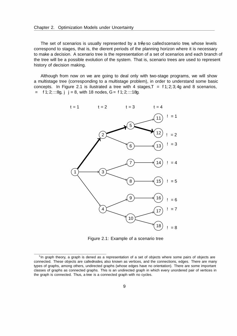
The set of scenarios is usually represented by a tree1, so called scenario tree, whose levelscorrespond to stages, that is, the different periods of the planning horizon where it is necessaryto make a decision. A scenario tree is the representation of a set of scenarios and each branch ofthe tree will be a possible evolution of the system. That is, scenario trees are used to representhistory of decision making.
Although from now on we are going to deal only with two-stage programs, we will showa multistage tree (corresponding to a multistage problem), in order to understand some basicconcepts. In Figure 2.1 is ilustrated a tree with 4 stages, T = 1, 2, 3, 4 and 8 scenarios,Ω = 1, 2, ...8, |Ω| = 8, with 18 nodes, G = 1, 2, ...18.
ω = 1
ω = 2
ω = 3
ω = 4
ω = 5
ω = 6
ω = 7
ω = 8
t = 1 t = 2 t = 3 t = 4
1
2
3
4
5
6
7
8
9
10
11
12
13
14
15
16
17
18
Figure 2.1: Example of a scenario tree
1In graph theory, a graph is defined as a representation of a set of objects where some pairs of objects areconnected. These objects are called nodes, also known as vertices, and the connections, edges. There are manytypes of graphs, among others, undirected graphs (whose edges have no orientation). There are some importantclasses of graphs as connected graphs. This is an undirected graph in which every unordered pair of vertices inthe graph is connected. Thus, a tree is a connected graph with no cycles.
9
2.2. Stochastic Linear Programming
In this tree we can see that the number of nodes in each post-node is equivalent to therealizations of uncertain parameters and in each stage there is enough information to make adecision. Notice that in the first stage there is only one node, called root node. A scenario is notone of each possible last state; but, as it can be seen in Figure 2.1, for example, ω = 2 is oneof the possible evolution of the system from the first stage to the last hypothetical one. Thus,each path from the root to a leaf is called scenario, a feasible realization of the uncertainty. Ineach node there is a variable to decide, that is, a decision that has to be made.
Once that the scenario tree is generated, it is necessary to extend the problem modelling, insuch a way that it will take the information from that tree. One option consists of solving thedeterministic problems according to each scenario ω ∈ Ω:
Zω = min cωXω
s.t. bω ≤ AωXω ≤ bω (2.3)
Xω ≥ 0
Based on the the previous model (2.3), the way of choosing an optimal solution is not clear.There can be feasible solutions in a scenario that could be non-feasible in another one.
However, the analysis of scenarios applied in a optimization problem provides feasible solu-tions under all the scenarios and optimal expected value over all of them. This happens, as wewill see later, due to the optimization of a linear combination of objective functions accordingto the set of scenarios.
2.2.2 Decisions and recourses
One of the most attractive aspects of the Stochastic Programming is the fact of including changesin the decisions to be taken, whenever information is available throughout the planning horizon.Furthermore, it has sense that, at the beginnig of a process with several decision stages, the firststage decisions must be taken. However, it does not have to happen the same with the decisionsof the other stages.
Definition 2.3. A solution is anticipative if there is a unique value for each variable, imple-mentable and independent from the random experiment. That is, decisions which must be takenbefore the uncertainties are resolved. On the contrary decisions that are taken after uncertaintyin the parameters has been resolved are called adaptative variables.
10
Chapter 2. Optimization Models under Uncertainty
All stochastic programs have some anticipative variables, since they would otherwise becomedeterministic. Stochastic programs that include both types of variables are generally calledrecourse models and according to the decision anticipativity, there is the following classification:
• Simple recourse model is that where all the decisions to take have to be fixed fromthe beginning, without any variation even though in the following periods of time moreinformation of each scenario can be reached. All the decisions have to be taken beforethe random experiment, and they belong to anticipative variables. This makes easier therepresentation and resolution of the model. However, conclusions can be far from the realresults, since new information reached in each stage is not used.
• Relatively complete recourse is the model where decisions of the first r stages aredetermined in the beginning (implementable periods), and the decisions of the rest areadjusted to the possible changes (non-implementable periods).
• Complete recourse model is that where all the decisions are adapted along the time,every time that information of the uncertain parameters is revealed; except for the variablesof the first stage, which do not depend on the scenario that happens. That is to say thatthe solution is formed by a set of only decisions for the first period and an optimal decisionfor each scenario. Complete recourse is often added to a model to ensure that no outcomecan produce infeasible results. It is the most interesting and useful model because thesolution provided is a set of decisions which get adapted to the information disposed ineach stage, allowing changes and optimizing the expected value of the objective function.
All the stochastic models used in this project are complete recourse models.
11
2.2. Stochastic Linear Programming
2.2.3 Non-anticipativity principle
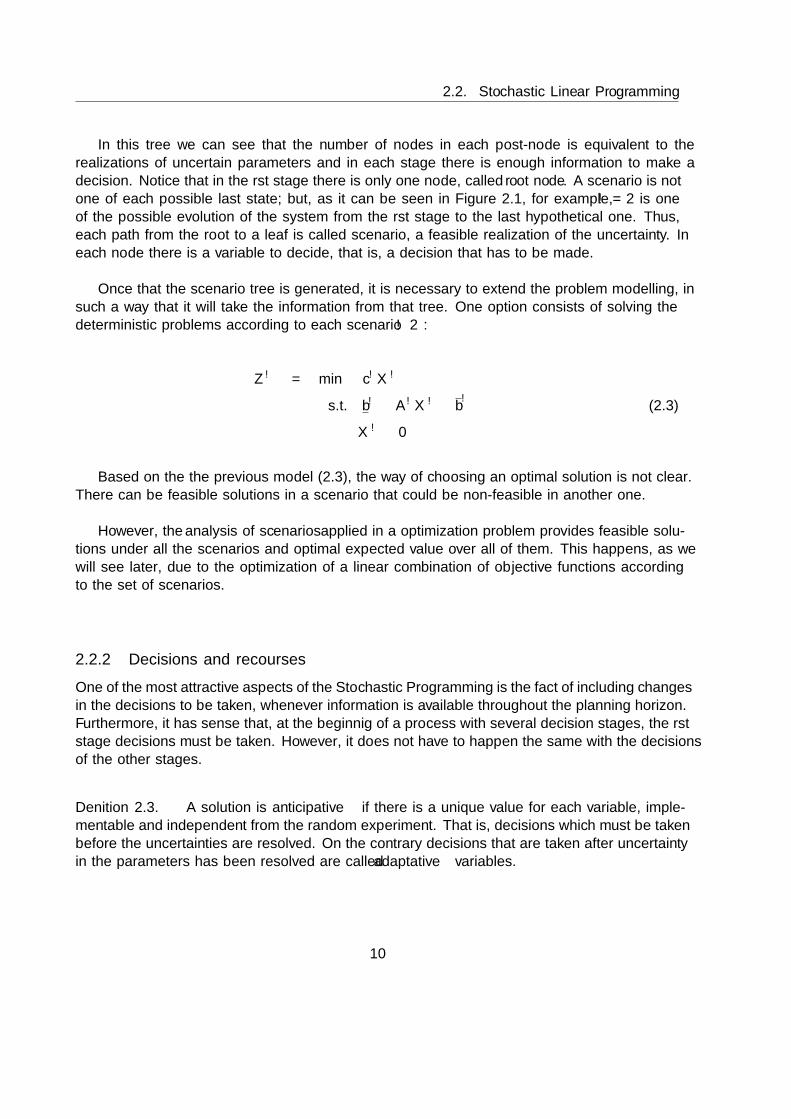
The principle of non-anticipativity (NAC) was introduced for two-stage problems in 1974 byWets, see [34] and restated by Rockafellar and Wets in 1991, see [27]. It states that if twoscenarios, ω and ω′, are equal according to the available information from the first to the rth
stage, then the decisions to take from those scenarios until this last stage have to be the same.Now, let us represent in Figure 2.8 the non-anticipativity principle according to the multistageexample corresponding to the tree in previous Figure 2.1 where decision variables in nodes insidethe same dashed ellipse must be the same. That is, there are six sets of variables that must bethe same.
ω = 1
ω = 2
ω = 3
ω = 4
ω = 5
ω = 6
ω = 7
ω = 8
t = 1 t = 2 t = 3 t = 4
Figure 2.2: Non-ancitipativity principle
All the decisions taken in the first stage must be the same under all the scenarios. At thethird stage, the decisions of first and second scenarios and seventh and eighth scenarios, mustbe the same, respectively.
According to the implicit or explicit representation of the NAC constraints, the models canbe defined in compact or splitting variable representation.
2.2.4 Two-Stage Model in Compact Representation
Stochastic problems were formulated for the first time in 1955 derivated from the linear opti-mization by Dantzig and Beale in [8] and [3], respectively. First stage is made up of a commonnode with the same information, while the second one consists of one node for each scenario.Therefore, first stage decisions will be the same and independent from the scenario, while seconddecisions are non-anticipative and depend on the scenario.
12
Chapter 2. Optimization Models under Uncertainty
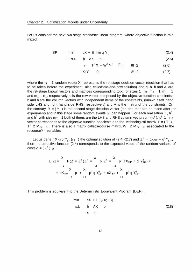
Let us consider the next two-stage stochastic linear program, where objective function is mini-mized:
SP = min cX + E[min q Y] (2.4)
s.t. b ≤ AX ≤ b (2.5)
hω ≤ TωX +WωY ω ≤ hω, ∀ω ∈ Ω (2.6)
X,Y ω ≥ 0, ∀ω ∈ Ω (2.7)
where the n1 × 1 random vector X represents the first-stage decision vector (decision that hasto be taken before the experiment, also called here-and-now solution) and c, b, b and A arethe first-stage known vectors and matrices corresponding to X, of sizes 1× n1, m1 × 1, m1 × 1and m1 × n1, respectively. c is the row vector composed by the objective function coefficients,b and b are the column vectors with independent items of the constraints, (known as left handside, LHS and right hand side, RHS, respectively) and A is the matrix of the constraints. Onthe contrary, Y = (Y ω) is the second stage decision vector (the one that can be taken after theexperiment) and in this stage some random events ω ∈ Ω can happen. For each realization ω, hω
and hω
with size m2×1 both of them, are the LHS and RHS column vectors, q = (qω), qω 1×n2
vector corresponds to the objective function coefficients and the technological matrix T = (Tω),Tω ∈ Mm2×n1 . There is also a matrix called recourse matrix, Wω ∈ Mm2×n2 associated to therecourse Y ω variables.
Let us define (XSP , (YωSP )ω∈Ω) the optimal solution of (2.4)-(2.7) and Zω = cXSP + qωY ω
SP ,then the objective function (2.4) corresponds to the expected value of the random variable ofcosts Z = (Zω)ω∈Ω.
E[Z] =∑ω∈Ω
P (Z = Zω)Zω =∑ω∈Ω
pωZω =∑ω∈Ω
pω(cXSP + qωY ωSP ) =
= cXSP
∑ω∈Ω
pω +∑ω∈Ω
pωqωY ωSP = cXSP +
∑ω∈Ω
pωqωY ωSP
This problem is equivalent to the Deterministic Equivalent Program (DEP):
min cX + E[Q(X,ω)]
s.t. b ≤ AX ≤ b (2.8)
X ≥ 0
13
2.2. Stochastic Linear Programming
where
Q(X,ω) = min qωY
s.t. hω − TωX ≤WωY ≤ hω − TωX, ∀ω ∈ Ω (2.9)
Y ≥ 0
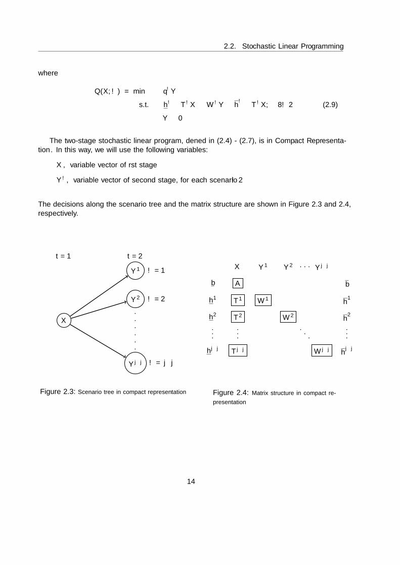
The two-stage stochastic linear program, defined in (2.4) - (2.7), is in Compact Representa-tion. In this way, we will use the following variables:
• X, variable vector of first stage
• Y ω, variable vector of second stage, for each scenario ω ∈ Ω
The decisions along the scenario tree and the matrix structure are shown in Figure 2.3 and 2.4,respectively.
ω = 1
ω = 2
ω = |Ω|
t = 1 t = 2
.
.
.
.
.
.
X
Y 1
Y 2
Y |Ω|
Figure 2.3: Scenario tree in compact representation
X Y 1 Y 2 . . . Y |Ω|
b
h1
h2
.
.
.
h|Ω|
.
.
....
b
h1
h2
.
.
.
h|Ω|
A
T 1
T 2
T |Ω|
W 1
W 2
W |Ω|
Figure 2.4: Matrix structure in compact re-
presentation
14
Chapter 2. Optimization Models under Uncertainty
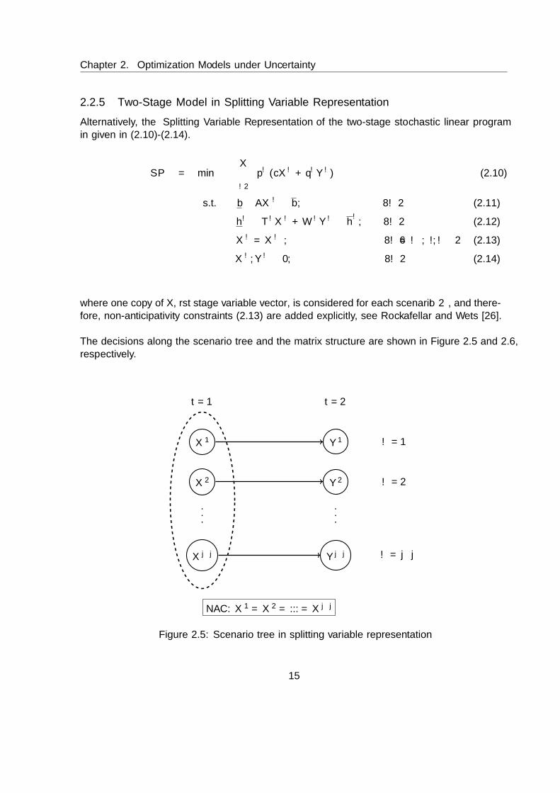
2.2.5 Two-Stage Model in Splitting Variable Representation
Alternatively, the Splitting Variable Representation of the two-stage stochastic linear programin given in (2.10)-(2.14).
SP = min∑ω∈Ω
pω (cXω + qωY ω) (2.10)
s.t. b ≤ AXω ≤ b, ∀ω ∈ Ω (2.11)
hω ≤ TωXω +WωY ω ≤ hω, ∀ω ∈ Ω (2.12)
Xω = Xω∗ , ∀ω 6= ω∗, ω, ω∗ ∈ Ω (2.13)
Xω, Y ω ≥ 0, ∀ω ∈ Ω (2.14)
where one copy of X, first stage variable vector, is considered for each scenario ω ∈ Ω, and there-fore, non-anticipativity constraints (2.13) are added explicitly, see Rockafellar and Wets [26].
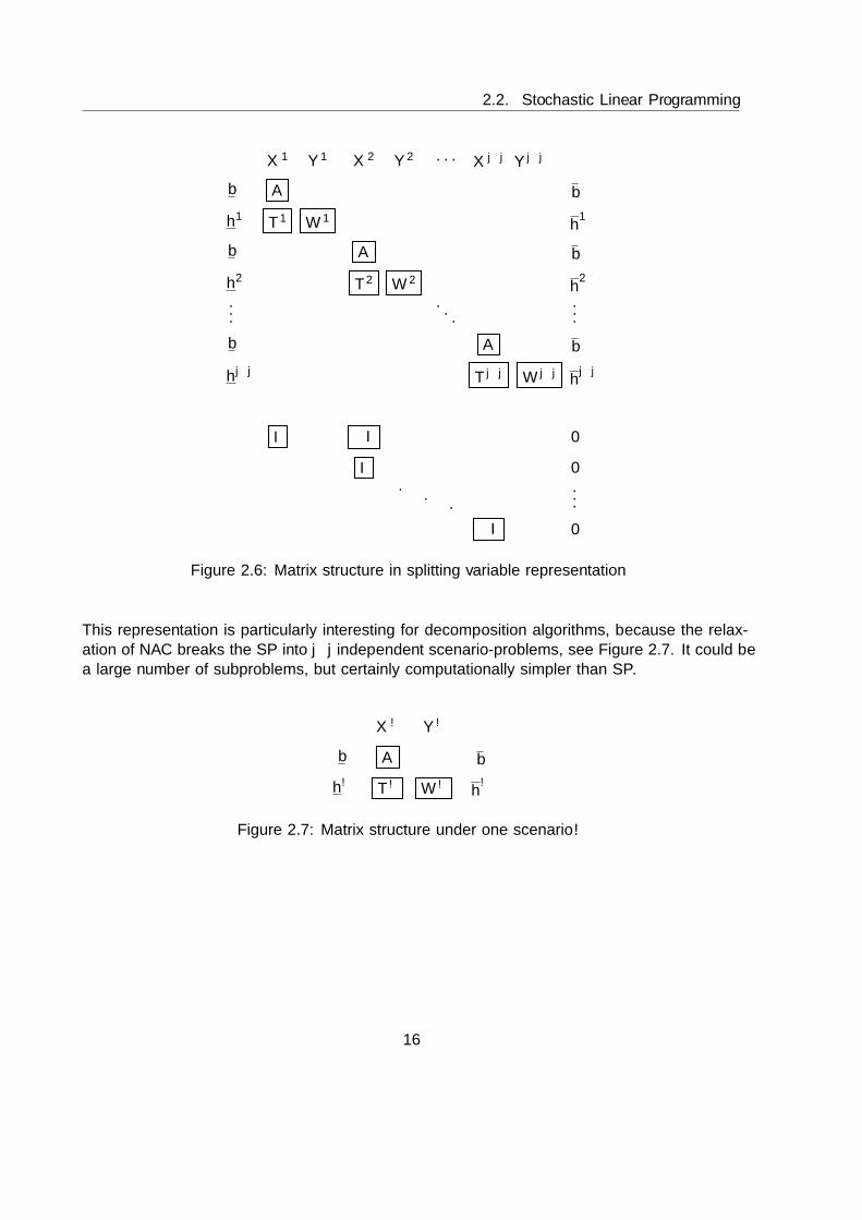
The decisions along the scenario tree and the matrix structure are shown in Figure 2.5 and 2.6,respectively.
ω = 1
ω = 2
ω = |Ω|
t = 1 t = 2
NAC: X1 = X2 = ... = X |Ω|
.
.
.
.
.
.
X1
X2
X |Ω|
Y 1
Y 2
Y |Ω|
Figure 2.5: Scenario tree in splitting variable representation
15
2.2. Stochastic Linear Programming
X1 X2 . . . X |Ω|Y 1 Y 2 Y |Ω|
b
b
b
h1
h2
...
h|Ω|
b
b
b
h1
h2
...
h|Ω|
0
0...
0
. . .
..
.
A
A
A
T 1
T 2
T |Ω|
W 1
W 2
W |Ω|
I −I
I
−I
Figure 2.6: Matrix structure in splitting variable representation
This representation is particularly interesting for decomposition algorithms, because the relax-ation of NAC breaks the SP into |Ω| independent scenario-problems, see Figure 2.7. It could bea large number of subproblems, but certainly computationally simpler than SP.
Xω Y ω
b
hω
b
hω
A
Tω Wω
Figure 2.7: Matrix structure under one scenario ω
16

Chapter 2. Optimization Models under Uncertainty
2.2.6 Some two-stage examples
Example 2.2. Let us remember the previous deterministic Diet Problem, in Example 2.1. Wehave two stage decisions:
• First stage decisions (X): amount of products to buy today for the warehouse, decisionsthat must be taken here and now.
• Second stage decisions (Y ω): amount of products needed to be purchased two weeks later,decisions depending on the scenario ω.
We will consider three cases, depending on the uncertainty sources:
Case 1 , where prices are now unknown for the second stage and depend on the selected market.
Case 2 , where nutrients and prices can be altered depending on the own-brand taken fromeach market, see Mulvey et al. 1955 [24] collected in Censor & Zenios 1997 [7].
Case 3 , where bounds on nutrient requirements depend on the characteristics of differentpotential clients.
Let us detail the three models, where stochasticity appears in several ways.
Case 1. Stochasticity in objective function coefficients, ξω = (qω).
Now, prices in two weeks are unknown. We have considered three markets where we cango shopping (ω1: Eroski, ω2: Simply and ω3: Mercadona). So, depending where we buy,the price of each product will be different (stochasticity). In this case, uncertainty is onlyconsidered in the cost.
Table 2.3: Price of each product depending on the market
First Stage Second Stagec qω Eroski (ω1) Simply (ω2) Mercadona (ω3)
Pasta c1 1.98 qω1 2.00 2.25 1.25Lentils c2 1.58 qω1 1.29 2.48 1.25
The scenario tree for modeling Case 1 is detailed in Figure 2.8.
(Y ω11 , Y ω1
2 )
(Y ω21 , Y ω2
2 )
(Y ω31 , Y ω3
2 )
(X1, X2) X
Y ω1
Y ω2
Y ω3
Eroski
Simply
Mercadona
Figure 2.8: Scenario tree for Case 1 and Case 2
17

2.2. Stochastic Linear Programming
Let us model the problem taking into account that all values are not equally likely. In Vito-ria city, there are 23 Eroski, 9 Simply and 4 Mercadona, i.e., (pω1 , pω2 , pω3) =
(2336 ,
936 ,
436
).
So, the model is given in (2.15):
min 1.98X1 + 1.58X2 +∑ω∈Ω
pω (qω1 qω2 )(Y ω1Y ω2
)subject to 142.5 ≤ 18X1 + 68.737X2
32775 ≤ 3530X1 + 3100X2 ≤ 45000 (2.15)
285 ≤ 18(X1 + Y ω1 ) + 68.737(X2 + Y ω
2 ), ∀ω ∈ 1, 2, 3
65550 ≤ 3530(X1 + Y ω1 ) + 3100(X2 + Y ω
2 ) ≤ 90000, ∀ω ∈ 1, 2, 3
Xi, Yωi ≥ 0, i ∈ 1, 2 and ω ∈ 1, 2, 3
where qωi values are given in Table 2.3.
Hence, the optimal solution of the problem (2.15) is given in Table 2.4, with a totalexpected cost of ZSP = 31963e:
Table 2.4: Optimal SP solution for Case 1
First Stage Second StageX Y ω ω1 ω2 ω3
Pasta X1 0 Y ω1 0 9285 0
Lentils X1 10573 Y ω2 10573 0 9285
Case 2. Stochasticity in objective function coefficients and recourse matrix, ξω =(qω,Wω).
Since we buy in different markets the nutrients of each product could also change. Let usshow all the nutrients expressed in Table 2.5:
Table 2.5: Nutrients of each product depending on the market
Wω Eroski (ω1) Simply (ω2) Mercadona (ω3)
Iron (mg)wω
11 17 16 19.0wω
12 68 69 68.6
Energy (kcal)wω
21 3540 3440 3590wω
22 2810 2810 2807
18

Chapter 2. Optimization Models under Uncertainty
Let us model the problem in this case:
min 1.98X1 + 1.58X2 +∑ω∈Ω
pω (qω1 qω2 )(Y ω1Y ω2
)subject to 142.5 ≤ 18X1 + 68.737X2
32775 ≤ 3530X1 + 3100X2 ≤ 45000 (2.16)
285 ≤ 18X1 + 68.737X2 + (wω11 wω12)(Y ω1Y ω2
), ∀ω ∈ 1, 2, 3
65550 ≤ 3530X1 + 3100X2 + (wω21 wω22)(Y ω1Y ω2
)≤ 90000, ∀ω ∈ 1, 2, 3
Xi, Yωi ≥ 0, i ∈ 1, 2 and ω ∈ 1, 2, 3
where (pω1 , pω2 , pω3) =(
2336 ,
936 ,
436
), qω values are defined in the Table 2.3 and nutrients
wωij in Table 2.5. Thus, the optimal solution of the problem (2.16) is given in Table 2.6,with a total expected cost of ZSP = 32977e:
Table 2.6: Optimal SP solution for Case 2
First Stage Second StageX Y ω ω1 ω2 ω3
Pasta X1 0 Y ω1 0 9285 9130
Lentils X1 10573 Y ω2 11664 0 0
Case 3. Stochasticity in second stage bounds, ξω = (hω, hω).
Let us define three different scenarios according to the age and sex of the person: ω1:100% women (20-49), ω2: 50% women (20-49) and 50% men (20-49), ω3: 100% men (20-49). In this case, LHS and RHS are uncertain where here-and-now decisions must be taken.
Let us show the bounds in the Table 2.7:
Table 2.7: Bounds according to each nutrient and scenario
hω 100% W(ω1) 50% W(ω2) 0% W(ω3)Min Iron hω1 494 387.20 285
Min Energy hω
2 65550 75744.45 85500Max Energy hω2 69000 79731.00 90000
19
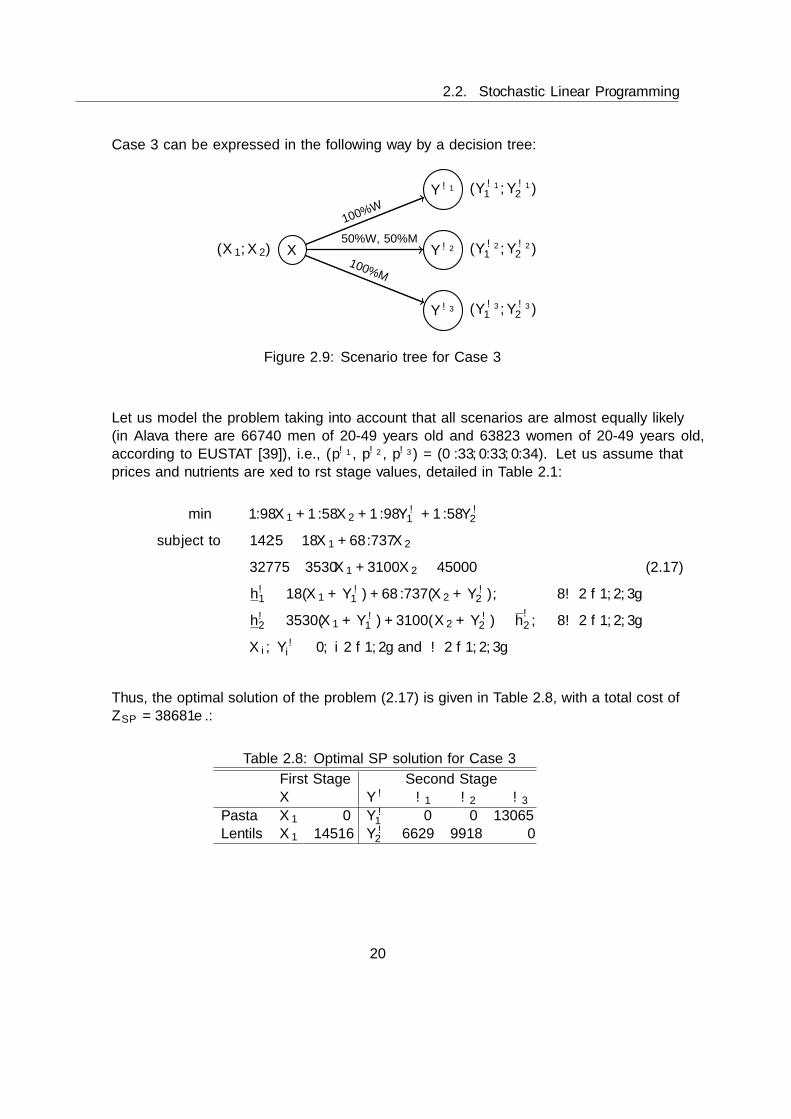
2.2. Stochastic Linear Programming
Case 3 can be expressed in the following way by a decision tree:
(Y ω11 , Y ω1
2 )
(Y ω21 , Y ω2
2 )
(Y ω31 , Y ω3
2 )
(X1, X2) X
Y ω1
Y ω2
Y ω3
100%W
50%W, 50%M
100%M
Figure 2.9: Scenario tree for Case 3
Let us model the problem taking into account that all scenarios are almost equally likely(in Alava there are 66740 men of 20-49 years old and 63823 women of 20-49 years old,according to EUSTAT [39]), i.e., (pω1 , pω2 , pω3) = (0.33, 0.33, 0.34). Let us assume thatprices and nutrients are fixed to first stage values, detailed in Table 2.1:
min 1.98X1 + 1.58X2 + 1.98Y ω1 + 1.58Y ω
2
subject to 142.5 ≤ 18X1 + 68.737X2
32775 ≤ 3530X1 + 3100X2 ≤ 45000 (2.17)
hω1 ≤ 18(X1 + Y ω1 ) + 68.737(X2 + Y ω
2 ), ∀ω ∈ 1, 2, 3
hω2 ≤ 3530(X1 + Y ω1 ) + 3100(X2 + Y ω
2 ) ≤ hω2 , ∀ω ∈ 1, 2, 3
Xi, Yωi ≥ 0, i ∈ 1, 2 and ω ∈ 1, 2, 3
Thus, the optimal solution of the problem (2.17) is given in Table 2.8, with a total cost ofZSP = 38681e.:
Table 2.8: Optimal SP solution for Case 3
First Stage Second StageX Y ω ω1 ω2 ω3
Pasta X1 0 Y ω1 0 0 13065
Lentils X1 14516 Y ω2 6629 9918 0
20
Chapter 3
The Value of Perfect Informationand the Stochastic Solution
Stochastic programs as, real world problems, are often computationally difficult to solve. Beforesolving the stochastic model, we could be tempted to solve simpler problems: for example, wecould simplify the real imprecise data, replacing the unknown parameters with expected valuesof those random variables and solve the obtained deterministic problem or alternatively, we couldsolve all related scenario submodels and compute the expectation of these different solutions.
The main issue about these alternatives is that sometimes the solution can be nearly optimal,totally inexact or even non implementable. The way to know if the simplified model is goodenough is calculating these two measures: the expected value of perfect information (EVPI) andthe value of the stochastic solution (VSS), see Birge & Louveaux 2011 [5].
In this chapter we will explain these two concepts for two-stage models. From Section 3.1to 3.3 there are shown essencial models, known as Wait-and-See (WS), Expected Value (EV)and Expected result of using Expected Value (EEV). Sections 3.4 and 3.5 provide the expectedvalue of perfect information and the value of stochastic solution. Some basic inequalities and therelationship between EVPI and VSS are given in Sections 3.6 and 3.7, respectively. For moregeneral definitions and inequalities, extended to the multistage stochastic model, see [9]. Theexample code is detailed in Appendix A.
21
3.1. Wait-and-See solution (WS)
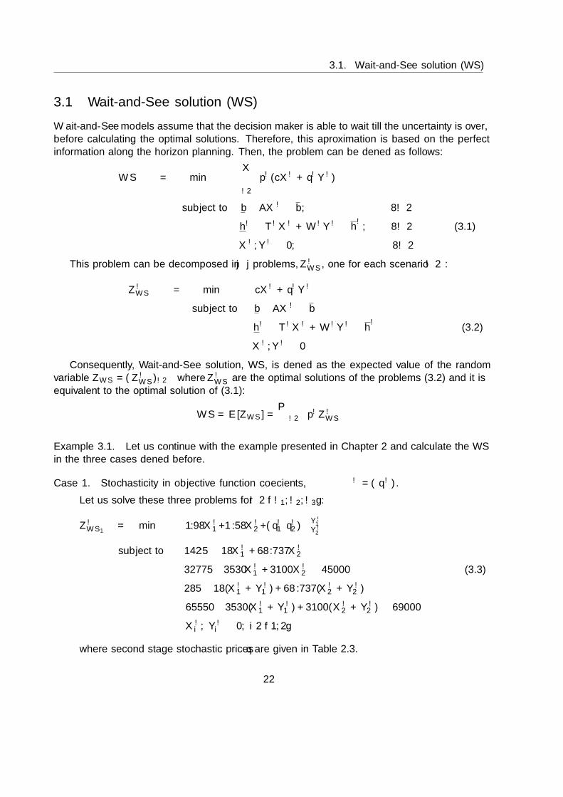
3.1 Wait-and-See solution (WS)
Wait-and-See models assume that the decision maker is able to wait till the uncertainty is over,before calculating the optimal solutions. Therefore, this aproximation is based on the perfectinformation along the horizon planning. Then, the problem can be defined as follows:
WS = min∑ω∈Ω
pω(cXω + qωY ω)
subject to b ≤ AXω ≤ b, ∀ω ∈ Ω
hω ≤ TωXω +WωY ω ≤ hω, ∀ω ∈ Ω (3.1)
Xω, Y ω ≥ 0, ∀ω ∈ Ω
This problem can be decomposed in |Ω| problems, ZωWS , one for each scenario ω ∈ Ω:
ZωWS = min cXω + qωY ω
subject to b ≤ AXω ≤ b
hω ≤ TωXω +WωY ω ≤ hω (3.2)
Xω, Y ω ≥ 0
Consequently, Wait-and-See solution, WS, is defined as the expected value of the randomvariable ZWS = (ZωWS)ω∈Ω where ZωWS are the optimal solutions of the problems (3.2) and it isequivalent to the optimal solution of (3.1):
WS = E[ZWS ] =∑
ω∈Ω pωZωWS
Example 3.1. Let us continue with the example presented in Chapter 2 and calculate the WSin the three cases defined before.
Case 1. Stochasticity in objective function coefficients, ξω = (qω).
Let us solve these three problems for ω ∈ ω1, ω2, ω3:
ZωWS1= min 1.98Xω
1 +1.58Xω2 +(qω1 qω2 )
(Y ω1Y ω2
)subject to 142.5 ≤ 18Xω
1 + 68.737Xω2
32775 ≤ 3530Xω1 + 3100Xω
2 ≤ 45000 (3.3)
285 ≤ 18(Xω1 + Y ω
1 ) + 68.737(Xω2 + Y ω
2 )
65550 ≤ 3530(Xω1 + Y ω
1 ) + 3100(Xω2 + Y ω
2 ) ≤ 69000
Xωi , Y
ωi ≥ 0, i ∈ 1, 2
where second stage stochastic prices q are given in Table 2.3.
22

Chapter 3. The Value of Perfect Information and the Stochastic Solution
Thus, the optimal solutions of the problems (3.3) according to each scenario are given inTable 3.1:
Table 3.1: Optimal WS solutions for Case 1
ω1 ω2 ω3
X∗1 0 0 0X∗2 10573 14513 10573Y ∗1 0 5822 9085Y ∗2 10573 0 0
Z∗ 30376e 36078e 28343e
It follows that the expected cost of products under the wait and see approach is
WS1 =23
36· 30376 +
9
36· 36078 +
4
36· 28343 = 31575e
Case 2. Stochasticity in objective function coefficients and recourse matrix, ξω =(qω,Wω).
Let us solve these three problems for ω ∈ ω1, ω2, ω3:
ZωWS2= min 1.98Xω
1 + 1.58Xω2 + (qω1 qω2 )
(Y ω1Y ω2
)subject to 142.5 ≤ 18Xω
1 + 68.737Xω2
32775 ≤ 3530Xω1 + 3100Xω
2 ≤ 45000 (3.4)
285 ≤ 18Xω1 + 68.737Xω
2 + (wω11 wω12)(Y ω1Y ω2
)65550 ≤ 3530Xω
1 + 3100Xω2 + (wω21 w
ω22)(Y ω1Y ω2
)≤ 69000
Xωi , Y
ωi ≥ 0, i ∈ 1, 2
where q values are defined in the Table 2.3 and nutrients W in Table 2.5.
23
3.1. Wait-and-See solution (WS)
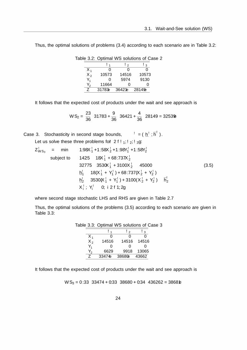
Thus, the optimal solutions of problems (3.4) according to each scenario are in Table 3.2:
Table 3.2: Optimal WS solutions of Case 2
ω1 ω2 ω3
X∗1 0 0 0
X∗2 10573 14516 10573
Y ∗1 0 5974 9130Y ∗2 11664 0 0Z∗ 31783e 36421e 28149e
It follows that the expected cost of products under the wait and see approach is
WS2 =23
36· 31783 +
9
36· 36421 +
4
36· 28149 = 32539e
Case 3. Stochasticity in second stage bounds, ξω = (hω, hω).
Let us solve these three problems for ω ∈ ω1, ω2, ω3:
ZωWS3= min 1.98Xω
1 +1.58Xω2 +1.98Y ω
1 +1.58Y ω2
subject to 142.5 ≤ 18Xω1 + 68.737Xω
2
32775 ≤ 3530Xω1 + 3100Xω
2 ≤ 45000 (3.5)
hω1 ≤ 18(Xω1 + Y ω
1 ) + 68.737(Xω2 + Y ω
2 )
hω2 ≤ 3530(Xω1 + Y ω
1 ) + 3100(Xω2 + Y ω
2 ) ≤ hω2Xωi , Y
ωi ≥ 0, i ∈ 1, 2
where second stage stochastic LHS and RHS are given in Table 2.7
Thus, the optimal solutions of the problems (3.5) according to each scenario are given inTable 3.3:
Table 3.3: Optimal WS solutions of Case 3
ω1 ω2 ω3
X∗1 0 0 0
X∗2 14516 14516 14516
Y ∗1 0 0 0Y ∗2 6629 9918 13065Z∗ 33474e 38680e 43662
It follows that the expected cost of products under the wait and see approach is
WS3 = 0.33 · 33474 + 0.33 · 38680 + 0.34 · 436262 = 38681e
24
Chapter 3. The Value of Perfect Information and the Stochastic Solution
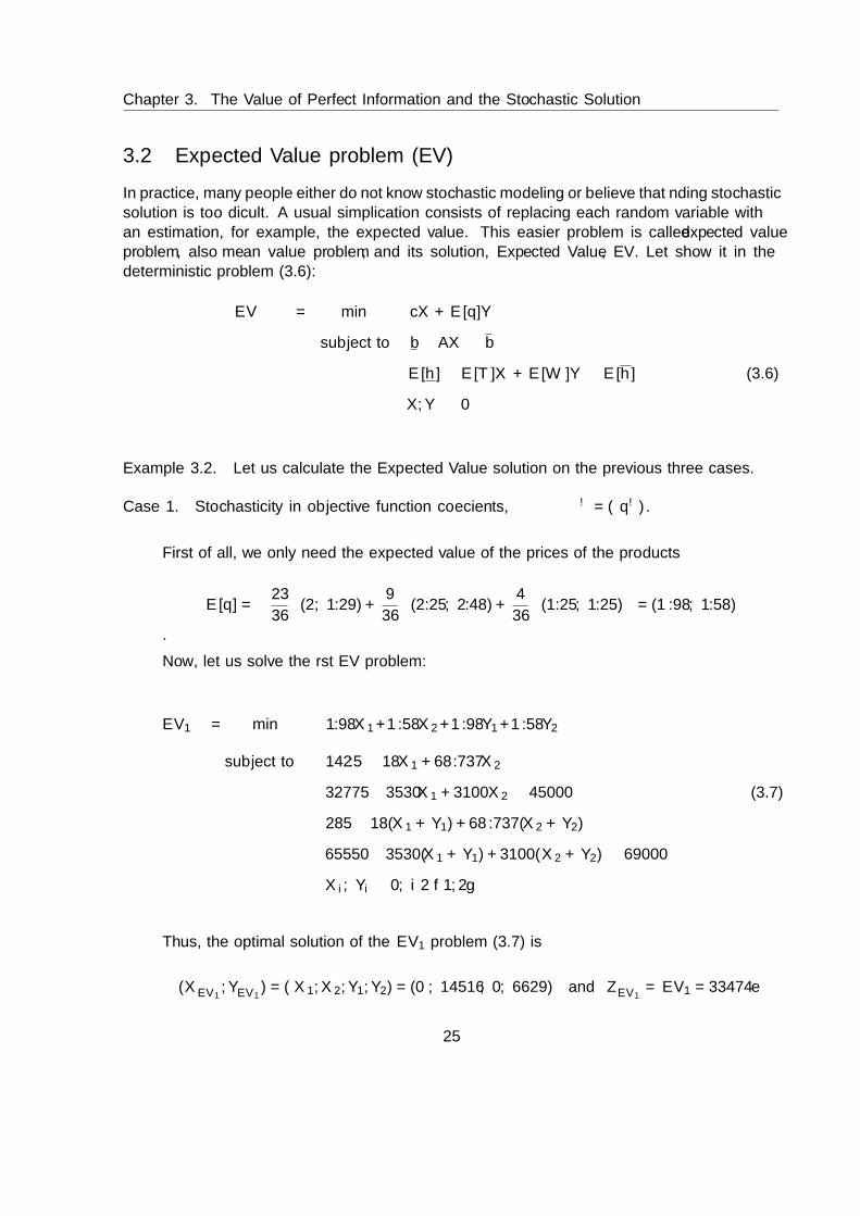
3.2 Expected Value problem (EV)
In practice, many people either do not know stochastic modeling or believe that finding stochasticsolution is too difficult. A usual simplification consists of replacing each random variable withan estimation, for example, the expected value. This easier problem is called expected valueproblem, also mean value problem, and its solution, Expected Value, EV. Let show it in thedeterministic problem (3.6):
EV = min cX + E[q]Y
subject to b ≤ AX ≤ b
E[h] ≤ E[T ]X + E[W ]Y ≤ E[h] (3.6)
X,Y ≥ 0
Example 3.2. Let us calculate the Expected Value solution on the previous three cases.
Case 1. Stochasticity in objective function coefficients, ξω = (qω).
First of all, we only need the expected value of the prices of the products
E[q] =
(23
36· (2, 1.29) +
9
36· (2.25, 2.48) +
4
36· (1.25, 1.25)
)= (1.98, 1.58)
.
Now, let us solve the first EV problem:
EV1 = min 1.98X1 +1.58X2 +1.98Y1 +1.58Y2
subject to 142.5 ≤ 18X1 + 68.737X2
32775 ≤ 3530X1 + 3100X2 ≤ 45000 (3.7)
285 ≤ 18(X1 + Y1) + 68.737(X2 + Y2)
65550 ≤ 3530(X1 + Y1) + 3100(X2 + Y2) ≤ 69000
Xi, Yi ≥ 0, i ∈ 1, 2
Thus, the optimal solution of the EV1 problem (3.7) is
(X∗EV1 , Y∗EV1
) = (X1, X2, Y1, Y2) = (0, 14516, 0, 6629) and Z∗EV1 = EV1 = 33474e
25
3.2. Expected Value problem (EV)
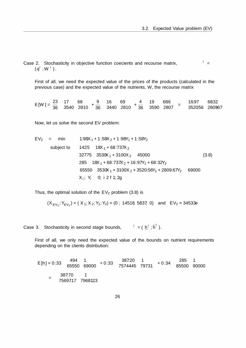
Case 2. Stochasticity in objective function coefficients and recourse matrix, ξω =(qω,Wω).
First of all, we need the expected value of the prices of the products (calculated in theprevious case) and the expected value of the nutrients, W, the recourse matrix
E[W] =23
36
(17 683540 2810
)+
9
36
(16 693440 2810
)+
4
36
(19 68.63590 2807
)=
(16.97 68.323520.56 2809.67
)
Now, let us solve the second EV problem:
EV2 = min 1.98X1 + 1.58X2 + 1.98Y1 + 1.58Y2
subject to 142.5 ≤ 18X1 + 68.737X2
32775 ≤ 3530X1 + 3100X2 ≤ 45000 (3.8)
285 ≤ 18X1 + 68.737X2 + 16.97Y1 + 68.32Y2
65550 ≤ 3530X1 + 3100X2 + 3520.56Y1 + 2809.67Y2 ≤ 69000
Xi, Yi ≥ 0, i ∈ 1, 2
Thus, the optimal solution of the EV2 problem (3.8) is
(X∗EV2 , Y∗EV2
) = (X1, X2, Y1, Y2) = (0, 14516, 5837, 0) and EV2 = 34533e
Case 3. Stochasticity in second stage bounds, ξω = (hω, hω).
First of all, we only need the expected value of the bounds on nutrient requirementsdepending on the clients distribution:
E[h] = 0.33
(494 ∞
65550 69000
)+ 0.33
(387.20 ∞
75744.45 79731
)+ 0.34
(285 ∞
85500 90000
)=
(387.70 ∞
75697.17 79681.23
)
26
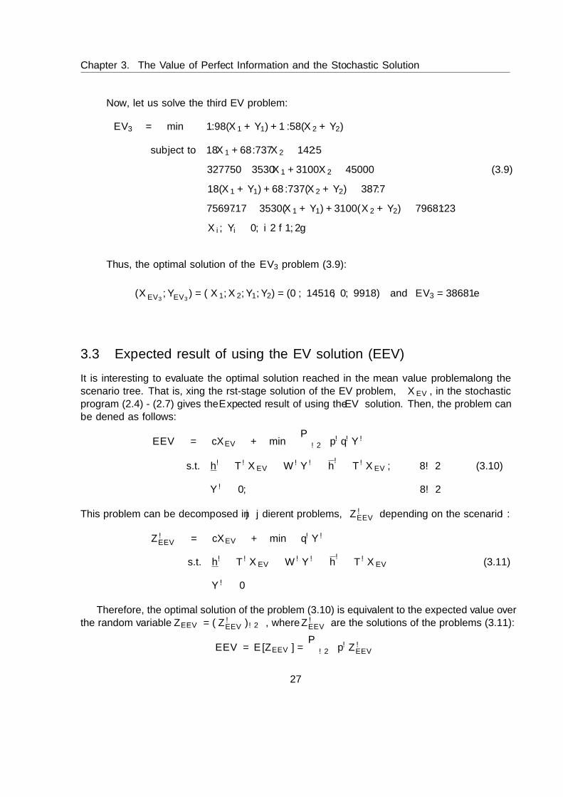
Chapter 3. The Value of Perfect Information and the Stochastic Solution
Now, let us solve the third EV problem:
EV3 = min 1.98(X1 + Y1) + 1.58(X2 + Y2)
subject to 18X1 + 68.737X2 ≥ 142.5
327750 ≤ 3530X1 + 3100X2 ≤ 45000 (3.9)
18(X1 + Y1) + 68.737(X2 + Y2) ≥ 387.7
75697.17 ≤ 3530(X1 + Y1) + 3100(X2 + Y2) ≤ 79681.23
Xi, Yi ≥ 0, i ∈ 1, 2
Thus, the optimal solution of the EV3 problem (3.9):
(X∗EV3 , Y∗EV3
) = (X1, X2, Y1, Y2) = (0, 14516, 0, 9918) and EV3 = 38681e
3.3 Expected result of using the EV solution (EEV)
It is interesting to evaluate the optimal solution reached in the mean value problem along thescenario tree. That is, fixing the first-stage solution of the EV problem, XEV , in the stochasticprogram (2.4) - (2.7) gives the Expected result of using the EV solution. Then, the problem canbe defined as follows:
EEV = cXEV + min∑
ω∈Ω pωqωY ω
s.t. hω − TωXEV ≤WωY ω ≤ hω − TωXEV , ∀ω ∈ Ω (3.10)
Y ω ≥ 0, ∀ω ∈ Ω
This problem can be decomposed in |Ω| different problems, ZωEEV depending on the scenario ω:
ZωEEV = cXEV + min qωY ω
s.t. hω − TωXEV ≤WωY ω ≤ hω − TωXEV (3.11)
Y ω ≥ 0
Therefore, the optimal solution of the problem (3.10) is equivalent to the expected value overthe random variable ZEEV = (ZωEEV )ω∈Ω, where ZωEEV are the solutions of the problems (3.11):
EEV = E[ZEEV ] =∑
ω∈Ω pωZωEEV
27
3.3. Expected result of using the EV solution (EEV)
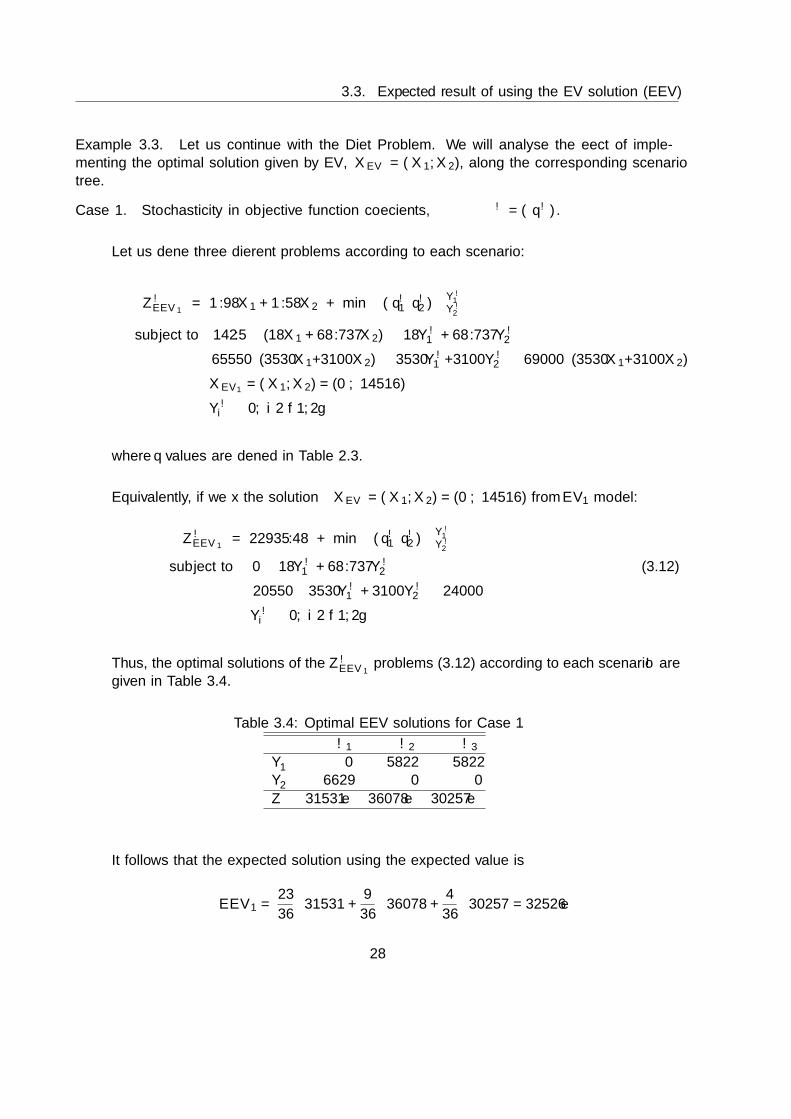
Example 3.3. Let us continue with the Diet Problem. We will analyse the effect of imple-menting the optimal solution given by EV, XEV = (X1, X2), along the corresponding scenariotree.
Case 1. Stochasticity in objective function coefficients, ξω = (qω).
Let us define three different problems according to each scenario:
ZωEEV1 = 1.98X1 + 1.58X2 + min (qω1 qω2 )(Y ω1Y ω2
)subject to 142.5− (18X1 + 68.737X2) ≤ 18Y ω
1 + 68.737Y ω2
65550−(3530X1+3100X2) ≤ 3530Y ω1 +3100Y ω
2 ≤ 69000−(3530X1+3100X2)
XEV1 = (X1, X2) = (0, 14516)
Y ωi ≥ 0, i ∈ 1, 2
where q values are defined in Table 2.3.
Equivalently, if we fix the solution XEV = (X1, X2) = (0, 14516) from EV1 model:
ZωEEV1 = 22935.48 + min (qω1 qω2 )(Y ω1Y ω2
)subject to 0 ≤ 18Y ω
1 + 68.737Y ω2 (3.12)
20550 ≤ 3530Y ω1 + 3100Y ω
2 ≤ 24000
Y ωi ≥ 0, i ∈ 1, 2
Thus, the optimal solutions of the ZωEEV1 problems (3.12) according to each scenario ω aregiven in Table 3.4.
Table 3.4: Optimal EEV solutions for Case 1
ω1 ω2 ω3
Y ∗1 0 5822 5822Y ∗2 6629 0 0
Z∗ 31531e 36078e 30257e
It follows that the expected solution using the expected value is
EEV1 =23
36· 31531 +
9
36· 36078 +
4
36· 30257 = 32526e
28
Chapter 3. The Value of Perfect Information and the Stochastic Solution
Case 2. Stochasticity in objective function coefficients and recourse matrix, ξω =(qω,Wω).
Let us define three different problems according to each scenario:
ZωEEV2 = 1.98X1 + 1.58X2 + min (qω1 qω2 )(Y ω1Y ω2
)subject to 142.5− (18X1 + 68.737X2) ≤ (wω11 w
ω12)(Y ω1Y ω2
)65550−(3530X1+3100X2) ≤ (wω21 w
ω22)(Y ω1Y ω2
)≤ 69000−(3530X1+3100X2)
XEV2 = (X1, X2) = (0, 14516)
Y ωi ≥ 0, i ∈ 1, 2
where q values are defined in the Table 2.3 and W in the Table 2.5.
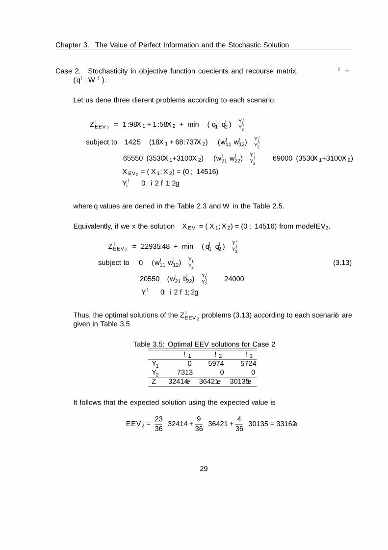
Equivalently, if we fix the solution XEV = (X1, X2) = (0, 14516) from model EV2.
ZωEEV2 = 22935.48 + min (qω1 qω2 )(Y ω1Y ω2
)subject to 0 ≤ (wω11 w
ω12)(Y ω1Y ω2
)(3.13)
20550 ≤ (wω21 bω22)(Y ω1Y ω2
)≤ 24000
Y ωi ≥ 0, i ∈ 1, 2
Thus, the optimal solutions of the ZωEEV2 problems (3.13) according to each scenario ω aregiven in Table 3.5
Table 3.5: Optimal EEV solutions for Case 2
ω1 ω2 ω3
Y ∗1 0 5974 5724Y ∗2 7313 0 0
Z∗ 32414e 36421e 30135e
It follows that the expected solution using the expected value is
EEV2 =23
36· 32414 +
9
36· 36421 +
4
36· 30135 = 33162e
29

3.3. Expected result of using the EV solution (EEV)
Case 3. Stochasticity in second stage bounds, ξω = (hω, hω).
Let us define three different problems according to each scenario:
ZωEEV3 = 1.98X1+1.58X2 + min 1.98Y ω1 +1.58Y ω
2
subject to hω1 − (18X1 + 68.737X2) ≤ 18Y ω1 + 68.737Y ω
2
hω2 − (3530X1 +3100X2) ≤ 3530Y ω1 +3100Y ω
2 ≤ hω2 − (3530X1 +3100X2)
XEV3 = (X1, X2) = (0, 14516)
Y ωi ≥ 0, i ∈ 1, 2
Equivalently, if we fix the solution XEV = (X1, X2) = (0, 14516) from EV3 model
ZωEEV3 = 22935.49 + min 1.98Y ω1 + 1.58Y ω
2
s.t. 0 ≤ 18Y ω1 + 68.737Y ω
2 (3.14)
hω2 − 45000 ≤ 3530Y ω1 + 3100Y ω
2 ≤ hω2 − 45000
Y ωi ≥ 0, i ∈ 1, 2
where h and h values are defined in the Table 2.7.
Thus, the optimal solutions of the ZωEEV3 problems (3.14) according to each scenario ωgiven in Table 3.6:
Table 3.6: Optimal EEV solutions for Case 3
ω1 ω2 ω3
Y ∗1 0 0 0Y ∗2 6629 9918 13065
Z∗ 33474e 38680e 43662
It follows that the expected solution using the expected value is
EEV3 = 0.33 · 33474 + 0.33 · 38680 + 0.34 · 43662 = 38681e
30
Chapter 3. The Value of Perfect Information and the Stochastic Solution
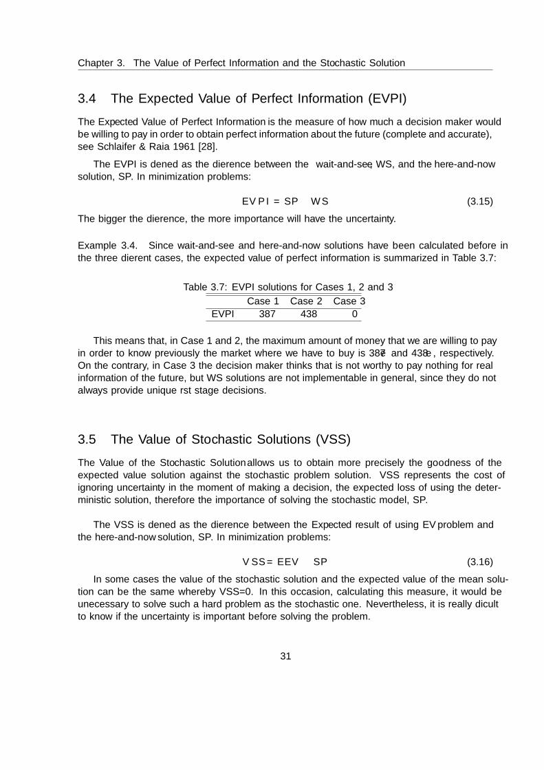
3.4 The Expected Value of Perfect Information (EVPI)
The Expected Value of Perfect Information is the measure of how much a decision maker wouldbe willing to pay in order to obtain perfect information about the future (complete and accurate),see Schlaifer & Raiffa 1961 [28].
The EVPI is defined as the difference between the wait-and-see, WS, and the here-and-nowsolution, SP. In minimization problems:
EV PI = SP −WS (3.15)
The bigger the difference, the more importance will have the uncertainty.
Example 3.4. Since wait-and-see and here-and-now solutions have been calculated before inthe three different cases, the expected value of perfect information is summarized in Table 3.7:
Table 3.7: EVPI solutions for Cases 1, 2 and 3
Case 1 Case 2 Case 3
EVPI 387 438 0
This means that, in Case 1 and 2, the maximum amount of money that we are willing to payin order to know previously the market where we have to buy is 387e and 438e, respectively.On the contrary, in Case 3 the decision maker thinks that is not worthy to pay nothing for realinformation of the future, but WS solutions are not implementable in general, since they do notalways provide unique first stage decisions.
3.5 The Value of Stochastic Solutions (VSS)
The Value of the Stochastic Solution allows us to obtain more precisely the goodness of theexpected value solution against the stochastic problem solution. VSS represents the cost ofignoring uncertainty in the moment of making a decision, the expected loss of using the deter-ministic solution, therefore the importance of solving the stochastic model, SP.
The VSS is defined as the difference between the Expected result of using EV problem andthe here-and-now solution, SP. In minimization problems:
V SS = EEV − SP (3.16)
In some cases the value of the stochastic solution and the expected value of the mean solu-tion can be the same whereby VSS=0. In this occasion, calculating this measure, it would beunecessary to solve such a hard problem as the stochastic one. Nevertheless, it is really difficultto know if the uncertainty is important before solving the problem.
31

3.6. Main Inequalities
If we remember the definition of EVPI, we can see that VSS seems similar to that. Thedifference is that EVPI is the maximum price that the decision maker should pay in order toknow the uncertainty, and VSS, on the contrary, is the real cost of ignoring it.
Example 3.5. Since the expected result of using the expected value and here-and-now solu-tions have been calculated before in the three different cases, the value of stochastic solution issummarized in Table 3.8.
Table 3.8: VSS solutions for Cases 1, 2 and 3
Case 1 Case 2 Case 3VSS 564 185 0
This means that Case 3 is the only one where it has not been worthy to calculate thestochastic solution. However, we cannot predict the result before the implementation of bothmodels. Notice that for Case 1 and Case 2, the result is remarkable.
3.6 Main Inequalities
The relations between the solutions and measures defined in the previous sections were estab-lished by Madansky in 1960 [23].
Proposition 3.1. For the minimization lineal models, the following inequalities are satisfied:
WS ≤ SP ≤ EEV (3.17)
Obviously, in the maximization models the inequalities are the opposite.
Proof. On one hand, since the optimal solution of the Stochastic Problem (2.4) - (2.7), alsoknown as Recourse Problem is feasible solution of the Wait-and-See problem (3.1), it is directlyproved the first part of the inequality: WS ≤ SP .
On the other hand, since the optimal solution of the Expected result of using EV problem(3.6) is feasible solution of the Stochastic Problem (2.4) - (2.7), the second inequality is reached:SP ≤ EEV
Example 3.6. We just need to compare the three values obtained before. As we can see inTable 3.9, Proposition 3.1 is verified in strict inequality for Cases 1 and 2:
Table 3.9: Proposition 3.1 verified for Cases 1, 2 and 3
WS SP EEVCase 1 31575 < 31963 < 32526Case 2 32539 < 32977 < 33162Case 3 38681 = 38681 = 38681
32
Chapter 3. The Value of Perfect Information and the Stochastic Solution
Proposition 3.2. In stochastic programs of minimization with fixed objective coefficients andfixed recourse matrix W :
EV ≤WS (3.18)
Proof. First, note that EV = min z(X,E(ξ)) and WS = Eξ[min z(X, ξ)]. This means that wecan base the proof in Jensen’s inequality, see Jensen 1906 [16]. It states that for any convexfunction f(ξ) of ξ: Ef(ξ) ≥ f(E(ξ)). Since ξ = (ξω)ω∈Ω, we need to show that f(ξ) =
Z(X∗, ξ) = ZξWS is a convex function of ξ.
Let us consider two different vectors, ξ1 and ξ2, and some convex combination: ξλ = λξ1 +(1 − λ)ξ2, λ ∈ (0, 1). Let Z∗1 = Z(X∗1 , ξ
1) and Z∗2 = Z(X∗2 , ξ2) be some optimal solutions of
mincX+E[min qξY ξ|hξ ≤ T ξX+W ξY ξ ≤ hξ, Y ξ ≥ 0], s.t. b ≤ AX ≤ b, X ≥ 0 for ξ = ξ1 and
ξ = ξ2, respectively. Then, λZ∗1 +(1−λ)Z∗2 is a feasible solution ofmincX+E[min qξλY ξλ | hξλ ≤
T ξλX+W ξλY ξλ ≤ hξ
λ
, Y ξλ ≥ 0], s.t. b ≤ AX ≤ b, X ≥ 0. Now, let Z∗λ be an optimal solutionof the last problem. We thus have
f(λξ1 + (1− λ)ξ2) = f(ξλ) = Z∗λ = min z(X,λξ1 + (1− λ)ξ2) ≤ Z(λ(X∗1 , ξ1) + (1− λ)(X∗2 , ξ
2))
≤ λZ(X∗1 , ξ1) + (1− λ)Z(X∗2 , ξ
2) = λZ∗1 + (1− λ)Z∗2 = λf(ξ1) + (1− λ)f(ξ2)
.This stablishes convexity of f(ξ), so according to Jensen’s inequality
EV = minX
z(X,E(ξ)) = f(E(ξ))≤≤≤ Ef(ξ) = Eξ[minX
z(X, ξ)] = WS
Notice that, the previous proposition is not true for all stochastic programs. Since we havealready seen, it can only be uncertainty in the independent terms of the constraints or in thetechnological matrix T . Consequently, it is enough choosing a stochastic program being q theonly non-fixed value. In this case, z would be a concave function of ξ, so Jensen’s inequalitycannot be applied.
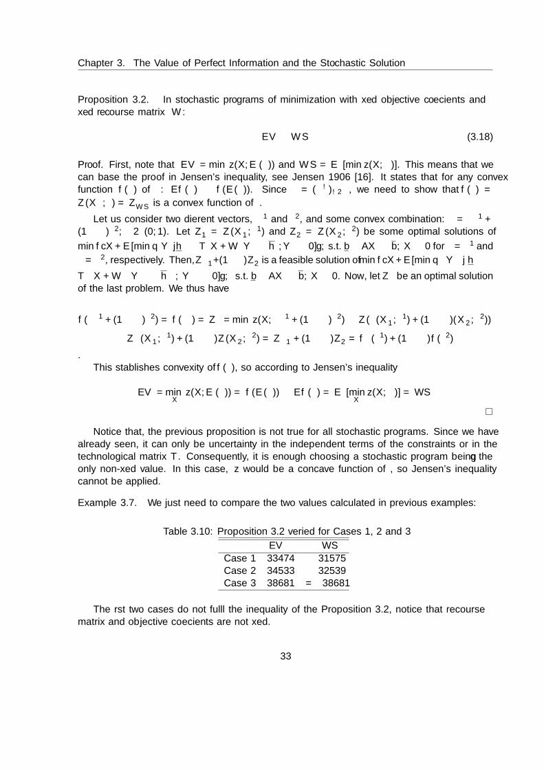
Example 3.7. We just need to compare the two values calculated in previous examples:
Table 3.10: Proposition 3.2 verified for Cases 1, 2 and 3
EV WS
Case 1 33474 31575Case 2 34533 32539Case 3 38681 = 38681
The first two cases do not fulfill the inequality of the Proposition 3.2, notice that recoursematrix and objective coefficients are not fixed.
33
3.7. The Relationship between EVPI and VSS
3.7 The Relationship between EVPI and VSS
The values of EVPI and VSS are usually different. This section describes the relationshipsbetween these two measures of uncertainty effects.
Proposition 3.3. For any stochastic program:
0 ≤ EV PI (3.19)
0 ≤ V SS (3.20)
Proof. It can be proved directly using Proposition 3.2.
Example 3.8. Note the satisfaction of Proposition 3.3 in Tables 3.7 and 3.8.
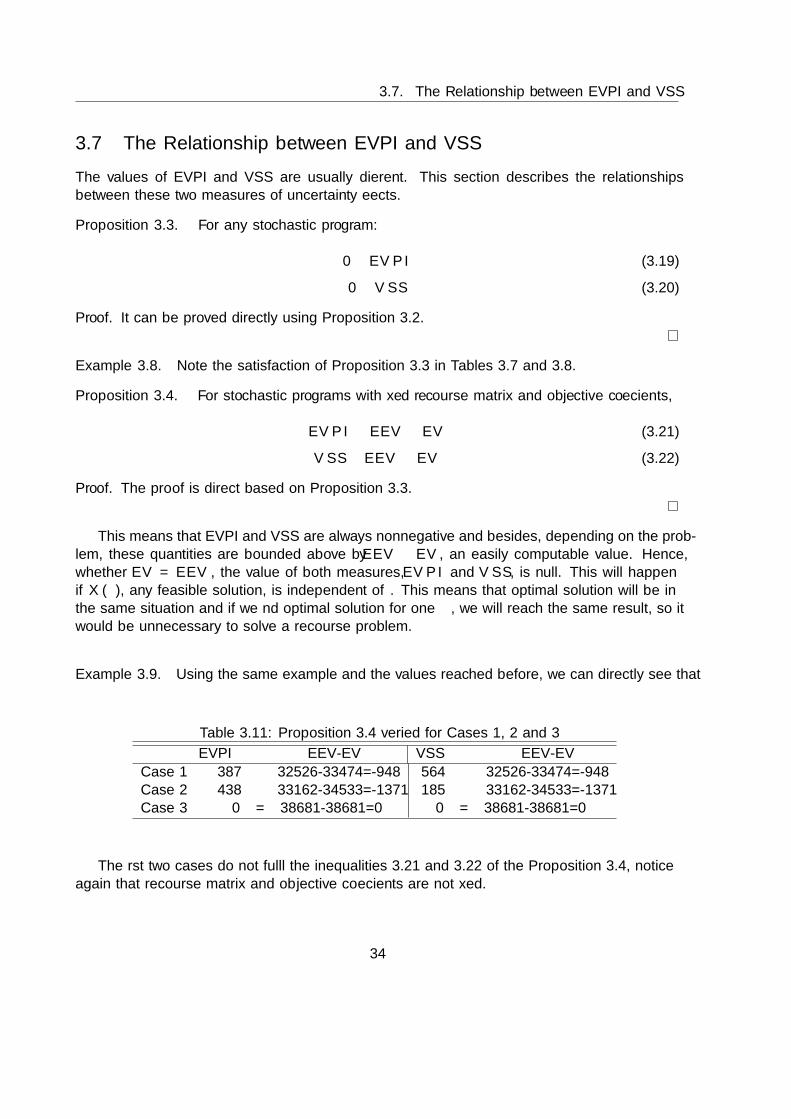
Proposition 3.4. For stochastic programs with fixed recourse matrix and objective coefficients,
EV PI ≤ EEV − EV (3.21)
V SS ≤ EEV − EV (3.22)
Proof. The proof is direct based on Proposition 3.3.
This means that EVPI and VSS are always nonnegative and besides, depending on the prob-lem, these quantities are bounded above by EEV − EV , an easily computable value. Hence,whether EV = EEV , the value of both measures, EV PI and V SS, is null. This will happenif X(ξ), any feasible solution, is independent of ξ. This means that optimal solution will be inthe same situation and if we find optimal solution for one ξ, we will reach the same result, so itwould be unnecessary to solve a recourse problem.
Example 3.9. Using the same example and the values reached before, we can directly see that
Table 3.11: Proposition 3.4 verified for Cases 1, 2 and 3
EVPI EEV-EV VSS EEV-EV
Case 1 387 32526-33474=-948 564 32526-33474=-948Case 2 438 33162-34533=-1371 185 33162-34533=-1371Case 3 0 = 38681-38681=0 0 = 38681-38681=0
The first two cases do not fulfill the inequalities 3.21 and 3.22 of the Proposition 3.4, noticeagain that recourse matrix and objective coefficients are not fixed.
34

Chapter 3. The Value of Perfect Information and the Stochastic Solution
Let us end this section by showing some other examples, see Birge & Louveaux 2011 [5], whereone of the two previous measures vanish.
Example 3.10. EV PI = 0 and V SS 6= 0
Let us define the following problem with the continuous random variable ξ uniformly dis-tributed over [1, 3] interval:
Z(X, ξ) = X1 + 4X2 + minY1 + 10Y +2 + 10Y −2 (3.23)
s.t. X1 +X2 = 1 (3.24)
Y1 + Y +2 − Y
−2 = ξ +X1 − 2X2 (3.25)
Xi ≥ 0, Y1 ≤ 2, Yi ≥ 0, i ∈ 1, 2 (3.26)
Notice that Y +2 + Y −2 = |Y2|, Y +
2 − Y−
2 = Y2, Y2 ∈ R. Since we want to keep Y+/−
2 as smallas possible in order to minimize Y1 + 10Y +
2 + 10Y −2 = Y1 + 10|Y2|, let us consider threedifferent cases:
• If Y2 = 0, then Y +2 − Y −2 = 0, Y1 = ξ + X1 − 2X2. In addition, since 0 ≤ Y1 ≤ 2,
0 ≤ ξ +X1 − 2X2 ≤ 2 (first region)
• If Y −2 = 0, then Y1 + Y +2 = ξ +X1 − 2X2, since Y1 ≤ 2, ξ +X1 − 2X2 ≤ 2 + Y +
2 . As it isa minimizing problem, Y +
2 = ξ + X1 − 2X2 − 2 and Y1 = 2. In this case, since Y +2 ≥ 0,
Y1 + Y +2 = 2 + Y +
2 ≥ 2, so, 2 + ξ +X1 − 2X2 − 2 = ξ +X1 − 2X2 ≥ 2 (second region)
• If Y +2 = 0, then Y1 − Y −2 = ξ + X1 − 2X2, since Y1 ≥ 0, ξ + X1 − 2X2 ≥ 0 − Y −2 . As
it is a minimizing problem, Y −2 = 2X2 − X1 − ξ and Y1 = 0. In this case, Y1 − Y −2 =2X2 −X1 − ξ ≥ 0, so, ξ +X1 − 2X2 ≤ 0 (third region)
That is,
Y ∗(X, ξ) = (Y1, Y+
2 , Y −2 ) =
(ξ +X1 − 2X2, 0, 0) if 0 ≤ ξ +X1 − 2X2 ≤ 2
(2, ξ +X1 − 2X2 − 2, 0), if ξ +X1 − 2X2 ≥ 2
(0, 0, 2X2 − ξ −X1), if ξ +X1 − 2X2 ≤ 0
Therefore,
Z(X, ξ) =
2X1 + 2X2 + ξ, if 0 ≤ ξ +X1 − 2X2 ≤ 2
−18 + 11X1 − 16X2 + 10ξ, if ξ +X1 − 2X2 ≥ 2
−9X1 + 2X2 − 10ξ, if ξ +X1 − 2X2 ≤ 0
(3.27)
35

3.7. The Relationship between EVPI and VSS
Given the first-stage constraint (3.24) X1 + X2 = 1, in the first region Z(X, ξ) = 2(X1 +X2) + ξ = 2 + ξ. Now, using the second-stage constraint (3.25), Y1 + Y +
2 − Y−
2 = ξ +X1− 2X2,Y1 + 10Y +
2 + 10Y −2 ≥ ξ + X1 − 2X2. So, for an optimal Y in the second and third region,applying (3.24), Z(X, ξ) ≥ X1 + 4X2 + (ξ + X1 − 2X2) = 2(X1 + X2) + ξ = 2 + ξ. Therefore,any X ∈ (X1, X2)|X1 + X2 = 1, X ≥ 0 is an optimal solution of the problem (3.23) - (3.26)for −X1 + 2X2 ≤ ξ ≤ −X1 + 2X2 + 2, and applying (3.24), equivalently,−X1 + 2(1−X1) ≤ ξ ≤ −X1 + 2(1−X1) + 2 ⇔ 2− 3X1 ≤ ξ ≤ 4− 2X1.
Since ξ follows a uniform distribution over [1,3], let us define three different cases:
• If ξ ≥ 1, 2−3X1 = 1⇔ X1 = 13 and X2 = 2
3 . Then, ξ ≤ 3, so, (13 ,
23) is an optimal solution
for all ξ.
• For X1 = 1, −1 ≤ ξ ≤ 1. Therefore, (1,0) is optimal in ξ ∈ 1.
• For X1 = 0, 2 ≤ ξ ≤ 4. Thus, (0,1) is optimal in ξ ∈ [2, 3].
Taking X∗(ξ) = (13 ,
23) for all ξ, since all the solutions will be the same, we can conclude
that WS = RP = 2 + ξ = 2 + 1+32 = 2 + 2 = 4, so EV PI = RP − WS = 0. On the
other hand, solving Z(X,E(ξ) = 2), we can reach another solution: X∗(2) = (0, 1), thenEV = min z(X,E(ξ)) = 2 + 2 = 4.
In that case, since ξ is uniform over [1, 3], P (ξ) = 1/2, ∀ξ ∈ [1, 2] and P (ξ) = 1/2, ∀ξ ∈ [2, 3].
Whereas, since ξ is a continuous random variable, E[X] =+∞∫−∞
xf(x)dx where f(x) is density
function and
EEV = Eξ≤2(24− 10ξ) + Eξ≥2(2 + ξ) =
∫ 2
1(24− 10ξ) · 1
2dξ +
∫ 3
2(2 + ξ) · 1
2dξ =
1
2
[24ξ − 10
ξ2
2
∣∣∣∣21
+ 2ξ +ξ2
2
∣∣∣∣32
]=
1
2
(24− 5 · 3 + 2 +
9
2− 2
)=
27
4.
Thus, V SS = EEV −RP = 274 − 4 = 11
4 .
36

Chapter 3. The Value of Perfect Information and the Stochastic Solution
Example 3.11. EV PI 6= 0 and V SS = 0
Let us consider again the previous problem (3.23)-(3.26), where ξ is discrete random variable,ξ ∈ 0, 3
2 , 3, with each event occurring with same probability, 13 . Taking into account the
optimal solution reached in the previous example:
• If ξ = 0, 2− 3X1 ≤ 0 ≤ 4− 3X1 ⇒
2− 3X1 ≤ 0
4− 3X1 ≥ 0
So, X∗(0) = X|X1 +X2 = 1, 23 ≤ X1 ≤ 4
3
• If ξ = 32 , 2− 3X1 ≤ 3
2 ≤ 4− 3X1 ⇒
1− 6X1 ≤ 0
5− 6X1 ≥ 0
So, X∗(32) = X|X1 +X2 = 1, 1
6 ≤ X1 ≤ 56
• If ξ = 3, 2− 3X1 ≤ 3 ≤ 4− 3X1 ⇒
−1− 3X1 ≤ 0
1− 3X1 ≥ 0
So, X∗(3) = X|X1 +X2 = 1, 0 ≤ X1 ≤ 13
Let us takeX∗(3/2) = (2/3, 1/3) as optimal solution of EV. Then, EV = Z((2/3, 1/3), 3/2) =2 + 3/2 = 7/2. Since for ξ ∈ 0, 3
2 we are in the first region and for ξ = 3 in the second one,
EEV = Eξ∈0, 32,3[Z((2/3, 1/3), ξ)] = 2 + Eξ∈0, 3
2[Y∗((2/3, 1/3), ξ)] + Eξ=3[Y ∗((2/3, 1/3), ξ)]
= 2 + Eξ∈0, 32[ξ] + Eξ=3
[2 + 10
(ξ +
2
3− 2
1
3− 2
)]= 2 +
1
3
(0 +
3
2
)+
1
312 =
13
2.
There is not just one optimal solution for the three cases, so RP 6= WS and therefore,EV PI 6= 0. In Wait-and-See solution, it is possible to get a different optimal solution dependingon the case (being all of them in the first region):
• X∗(0) = (1, 0), so Z((1, 0), 0) = 2 + 0 = 2
• X∗(3/2) = (1/2, 1/2), so Z((1/2, 1/2), 3/2) = 2 + 32 = 7
2
• X∗(3) = (0, 1), so Z((0, 1), 3) = 2 + 3 = 5
Hence,
WS =1
3· 2 +
1
3· 7
2+
1
3· 5 =
7
2.
So that we can reach the recourse solution, we will solve the stochastic program minE[Z(X, ξ)],so (2/3, 1/3) is the optimal solution of SP. Thus
EV = 7/2 = WS ≤ RP = 13/2 = EEV
and EV PI = RP −WS = 3 while V SS = EEV −RP = 0.
37

3.7. The Relationship between EVPI and VSS
38
Chapter 4
An Application in the Third Sector:Hazia Project
In this chapter a third sector application is described, implemented and analysed. The thirdsector, also known as social economy or community sector, is the economic sector undertakenby non-governmental organizations and other non-profit organizations.
The computational experience has been carried out on a UPV/EHU server with the followingfeatures: 64 bits Linux Debian 8.3. operative system, Intel E5-2670 processor and 20 cores, 40such virtualized. It also contains two hard drives: a RAID one with 300Gb and a solid statewith 120Gb (128Gb usable RAM).
The application is detailed in Appendix B. The codes are implemented with the modelingsystem for mathematical programming and optimization, GAMS 22.8.1 [41] and solved by theoptimizer solver CPLEX 11.1.1 [43]. The figures shown in this chapter have been obtained fromthe software environment for statistical computing and graphics, R-project [42].
Section 4.1 explains the context, Section 4.2 details the models, Section 4.3 includes all thedatasets needed for the model, Section 4.4 shows and analyses the results and Section 4.5 con-cludes.
4.1 Background
Sortarazi association [37], with recognition of Public Utility, was created in 1991 in the neigh-bourhood of San Francisco (Bilbao) in order to promote and contribute in the developmentof men and women in risk of social exclusion. Nowadays, it is extended to some other placesin Bizkaia, above all, in areas or neighbourhoods with socio-economical disadvantages, such asErandio, Getxo, Leioa, Astrabudua and Bilbao.
39

4.2. Diet stochastic models and alternative models
Sortarazi has several social projects, but we will focus in the one called Hazia project. Itpretends to help people and families improving their personal, familiar and social situation sothat they can improve their social and labor integration possibilities. They want to treat specif-ically: orientation and emotional support, individual and group psicological support, advance ofmunicipal help, material basic necessities (payment of gas, water and electricity supply, rents,school expenses) and basic necessities of feeding (food delivery and baby set). Among all theservices that are offered, in this project we will be dealing with the last support, food delivering,for those families that do not receive social benefits neither any other income.
In 2013 there were 545 families assisted, adding up to 1404 people. Every family unit issummoned monthly making a week delivery in tuesday, wednesday or thursday in the afternoon,where there can be assisted no more than 40 families per day.
The service continues thanks mainly to the Food Bank of Bizkaia, public and private sup-port, as well as individual cooperations.
4.2 Diet stochastic models and alternative models
Let us explain the application model, based on the well known Diet Problem where the horizonplanning is a month. As we have said before, there are two main goals in this application: (1)minimize the cost of a monthly nutrition of around 900 users, supplying the maximum of thenutrients requirement and (2) compute the minimum cost of a monthly nutrition of around 900users, improving the percentage of the nutrients requirement, without exceeding the budget.The nutrients analized are those which appear in the product labels: energy, fat, saturated fat(SF), carbohydrates (CH), fibre, proteins and salt.
Notice that we can consider three sources of uncertainty: prices and nutrients can changeaccording to the available brand in the market and the number of users can vary slightly fromthe expected demand.
The problem is composed by the following sets, parameters and variables:
Sets:
Ω, the set of scenarios which represents uncertainty
I, the set of products supplied by Hazia Project and
J , the set of nutrients analized from each product
40
Chapter 4. An Application in the Third Sector: Hazia Project
Deterministic parameters:
c = (ci), the price vector of the products i needed to be purchased in the initial periodof planning horizon, i ∈ I
A = (aij), the first stage constraints matrix of the nutrient j corresponding to the producti, i ∈ I and j ∈ J
T = (tij), the technological matrix of the nutrient j of the product i, i ∈ I and j ∈ Jb0 = (b0j ), the minimum monthly nutrients requirement for a healthy diet per person
b0
= (b0j ), the maximum monthly nutrients requirement for a healthy diet per person
N0, the average amount of people demanding the service monthly
b = (bj), the minimum nutrients requirement for a healthy diet monthly for N0 people,
b = b0 ·N0
b = (bj), the maximum nutrients requirement for a healthy diet monthly for N0 people,
b = b0 ·N0
α1, the minimum percentage of the requirement that must be satisfied in the initial periodof planning horizon
α2, the maximum percentage of the requirement that must be satisfied in the initialperiod of planning horizon
β = (βj), the minimum percentages of nutrient requiment j that must be satisfied for theplanning horizon
δ = (δi), δ′ = (δ′i), ratios for determining lower bounds for X and Y variables, respectively
Z0, the initial budget
Stochastic parameters:
p = (pω), the likelihood of each scenario ω, ω ∈ Ω
q = (qωi ), the price vector of the products i needed to be purchased in the middle ofplanning horizon, i ∈ I
W = (wωij), the recourse matrix of the nutrient j of the product i, i ∈ I and j ∈ JN = (Nω), the amount of people demanding the service in a month, ω ∈ Ω
h = (hωj ), the minimum nutrients requirement j for a healthy diet, j ∈ J and ω ∈ Ω,
h = b0 ·Nh = (h
ωj ), the maximum nutrients requirement j for a healthy diet, j ∈ J and ω ∈ Ω,
h = b0 ·N
Variables:
X = (Xi), the vector of the products i needed to be purchased at the initial period ofplanning horizon, i ∈ I
Y = (Y ωi ), the vector of the products i needed to be purchased in the middle of planning
horizon depending on the scenario ω, i ∈ I and ω ∈ Ω
41

4.2. Diet stochastic models and alternative models
The two-stage diet Stochastic Problem reads as follows:
min∑i∈I
ciXi +∑ω∈Ω
pω
(∑i∈I
qωi Yωi
)(4.1)
s.t. α1 · bj ≤∑i∈I
aijXi ≤ α2 · bj , ∀j ∈ J (4.2)
βj · hωj ≤∑i∈I
tijXi +∑i∈I
wωijYωi ≤ h
ωj , ∀j ∈ J, ∀ω ∈ Ω (4.3)
∑i∈I
ciXi +∑ω∈Ω
pω
(∑i∈I
qωi Yωi
)< Z0 (4.4)
Xi ≥ δi ·∑i∈I
Xi, ∀i ∈ I (4.5)
Y ωi ≥ δ′i ·
∑i∈I
Yωi , ∀i ∈ I, ∀ω ∈ Ω (4.6)
Xi, Yωi ≥ 0, ∀i ∈ I, ∀ω ∈ Ω (4.7)
where (4.1) represents the objective function to optimize, the minimum cost, (4.2) is the set ofconstraints of the first stage, (4.3) are the global nutrient requirement, (4.4) defines the budgetlimitation, (4.5) and (4.6) denote the bounds for the variables X and Y ω, where Xi and Y
ωi are
solutions obtained from non-balanced models, respectively and (4.7) declares the non-negativeof the variables.
We will consider four models, according to different goals:
Model 1.a. The goal is to obtain the product distribution that minimizes the cost in order tosatisfy entirely the nutrition requirement. In this case, Z0 = +∞, βj = 1,∀j ∈ J andδi = δ′i = 0, ∀i ∈ I. That is, (4.4)-(4.6) are inactive.
Model 2.a. The goal is to improve the association standard nutritional bounds, without ex-ceeding the initial budget, Z0. δi = δ′i = 0,∀i ∈ I, that is, (4.5) and (4.6) are inactive.
Model 1.b. The goal is the same as Model 1.a., but mantaining a balanced diet. In this case,(4.5) is applied, but Z0 =∞, that is, (4.4) is inactive.
Model 2.b. The goal is the same as Model 1.b., but mantaining a balanced diet. In this case,(4.5) is applied. All the constraints are active.
42

Chapter 4. An Application in the Third Sector: Hazia Project
For comparison purposes, we will also calculate the problems WS(4.8), EV(4.9) and EEV(4.10):
• WS = Eξ[min z(X, ξ)] = Eξ[Z(X∗(ξ), ξ)],
where X∗(ξ) corresponds to the optimal solution of WS (4.8)
• EV = min z(X, ξ),
where ξ∗ = E[ξ] (4.9)
• EEV = Eξ[Z(X∗(ξ∗), ξ)],
where X∗(ξ∗) corresponds to the optimal solution of EV (4.10)
4.3 Dataset
The data for the models has been collected from the Sortarazi’s storehouse and from standardnutritional references.
4.3.1 First stage prices and nutrients
The values of energy, macronutrients and minerals (Na) for 100g of each product, have beentaken from AESAN/BEDCA, the spanish database of food composition (2010), see [36], takinginto account the product sets, sizes and prices of the association warehouse, see Table 4.1. Theseare, the values for first stage A matrix, second stage T technology matrix and c vector.
Table 4.1: Energy, macronutrients and minerals of each product by BEDCA
Reference BEDCA SizeEnergy Fat SF CH Fibre Proteins Salt Price
(kcal) (g) (g) (g) (g) (g) (g) (e)2541 Oil 1l 8870.00 999.00 106.20 0.00 0.00 0.00 0.00 2.851117 Pasta 500g 1765.00 7.25 0.95 354.50 25.00 62.50 0.06 1.031020 Chickpea 1kg 3360.00 63.00 4.28 492.50 149.70 193.10 0.75 2.892675 Maria Biscuits 200g 958.00 38.00 19.40 138.00 6.20 15.60 1.09 0.462660 Rice 1kg 3870.00 9.00 2.10 860.00 14.00 70.00 0.15 2.052648 Cacao 1kg 3900.00 40.00 2.50 810.20 35.00 58.80 12.60 2.092131 Tuna 80g 164.00 9.68 1.44 0.00 0.00 19.05 0.74 0.752632 Sardine 115g 272.55 18.11 3.22 0.00 0.00 27.52 1.05 1.852560 Fried Tomato 390g 327.60 24.96 2.42 20.28 6.24 5.85 3.32 0.662493 Whole milk 1l 650.00 38.00 23.00 47.00 0.00 30.60 1.20 0.951109 Coffee 250g 277.50 0.75 0.30 20.00 0.00 46.25 0.25 1.20
43
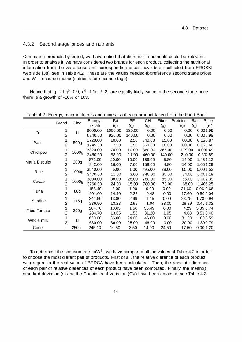
4.3. Dataset
4.3.2 Second stage prices and nutrients
Comparing products by brand, we have notified that difference in nutrients could be relevant.In order to analyse it, we have considered two brands for each product, collecting the nutritionalinformation from the warehouse and corresponding prices have been collected from EROSKIweb side [38], see in Table 4.2. These are the values needed for q0 (reference second stage price)and Wω recourse matrix (nutrients for second stage).
Notice that qω ∈ q0 · 0.9, q0 · 1.1, ω ∈ Ω are equally likely, since in the second stage pricethere is a growth of -10% or 10%.
Table 4.2: Energy, macronutrients and minerals of each product taken from the Food Bank
Brand SizeEnergy Fat SF CH Fibre Proteins Salt Price
(kcal) (g) (g) (g) (g) (g) (g) (e)
Oil1
1l9000.00 1000.00 130.00 0.00 0.00 0.00 0.00 1.99
2 8240.00 920.00 140.00 0.00 0.00 0.00 0.00 3.99
Pasta1
500g1720.00 10.00 2.50 340.00 15.00 60.00 0.15 0.87
2 1745.00 7.50 1.50 350.00 18.00 60.00 0.15 0.60
Chickpea1
1000g3320.00 70.00 10.00 360.00 266.00 179.00 0.00 1.49
2 3480.00 58.00 11.00 460.00 140.00 210.00 0.30 2.89
Maria Biscuits1
200g872.00 20.00 10.00 156.00 5.80 14.00 1.46 1.12
2 842.00 16.00 7.60 158.00 4.80 14.00 1.66 1.29
Rice1
1000g3540.00 5.00 1.00 795.00 28.00 65.00 0.00 1.52
2 3470.00 11.00 3.00 740.00 35.00 84.00 0.00 1.19
Cacao1
1000g3800.00 38.00 28.00 780.00 85.00 65.00 0.00 2.39
2 3760.00 24.00 15.00 780.00 78.00 68.00 1.40 6.25
Tuna1
80g158.40 8.00 1.20 0.00 0.00 21.60 0.96 0.66
2 201.60 14.40 2.32 0.48 0.00 17.60 0.50 2.04
Sardine1
115g241.50 13.80 2.99 1.15 0.00 28.75 1.73 0.94
2 236.90 13.23 2.99 1.04 23.00 28.29 0.46 1.32
Fried Tomato1
390g284.70 13.65 1.56 35.49 0.00 4.29 5.85 0.74
2 284.70 13.65 1.56 31.20 1.95 4.68 3.51 0.40
Whole milk1
1l630.00 36.00 24.00 46.00 0.00 31.00 1.00 0.59
2 630.00 36.00 25.00 46.00 0.00 30.00 1.30 0.79Coffee - 250g 245.10 10.50 3.50 14.00 24.50 17.50 0.00 1.20
To determine the scenario tree for Wω, we have compared all the values of Table 4.2 in orderto choose the most different pair of products. First of all, the relative difference of each productwith regard to the real value of BEDCA have been calculated. Then, the absolute differenceof each pair of relative differences of each product have been computed. Finally, the mean (x),standard deviation (s) and the Coefficients of Variation (CV) have been obtained, see Table 4.3.
44

Chapter 4. An Application in the Third Sector: Hazia Project
Table 4.3: Selection of the most different products
Product x s CV
Oil 4.09 4.54 111.16Pasta 22.77 33.47 146.95Chickpea 27.87 26.59 95.40Maria Biscuits 11.77 11.96 101.58Rice 14.86 17.24 116.02Cacao 35.62 61.55 172.82Tuna 32.64 54.05 165.57Sardine 4.34 7.02 161.84Fried Tomato 19.62 24.25 123.62Whole milk 4.30 7.41 172.35
The criteria for selecting a pair of products to be considered in the scenario tree is as fol-lows. The lower the CV, the bigger the convenience of introducing the product nutrients in thescenario tree. In effect, the bigger the mean and the smaller the standard deviation, the morerelevant to take into account the differences. The five most different pairs of products, accordingto the lowest CV are Chickpea, Maria Biscuits, Oil, Rice and Fried Tomato.
4.3.3 Nutricional bounds
For determing bounds on nutritional requirements, we must take into account nutritive proper-ties. For first stage, around half of the requirements should be satisfied (determined by α1, α2
parameters near to 0.5). Moreover, for the second stage (almost) all of them, where low boundis fixed by β parameter near to 1.
As stated in BEDCA [36], fat, like carbohydrates and proteins, is considered a majormacronutrient for the body due to the energy they provide (9Kcal/g) and the quantity of func-tions of the organism in which participates. However, it should be only 30%-35% of the energy.It is not only that important the quantity but the quality of the fat. So, less than 7%-8% of thefat must be saturated.
Carbohydrates contain monosaccharides (glucose, fructose and galactose), disaccharides (sac-arose, lactose) and polisaccharides (starch and glycogen). They provide 4Kcal/g and they shouldbe 50%-60% of the calories consumed per day.
Fibre is a plant material that cannot be digested but helps us to digest other food. For ahealthy diet, it must be consumed more than 14g/1000Kcal.
Protein is a building material of our skin, bones, muscles and other tissues in the body amongother things. In fact, the vast majority of the biological functions are carried out by proteins.
45
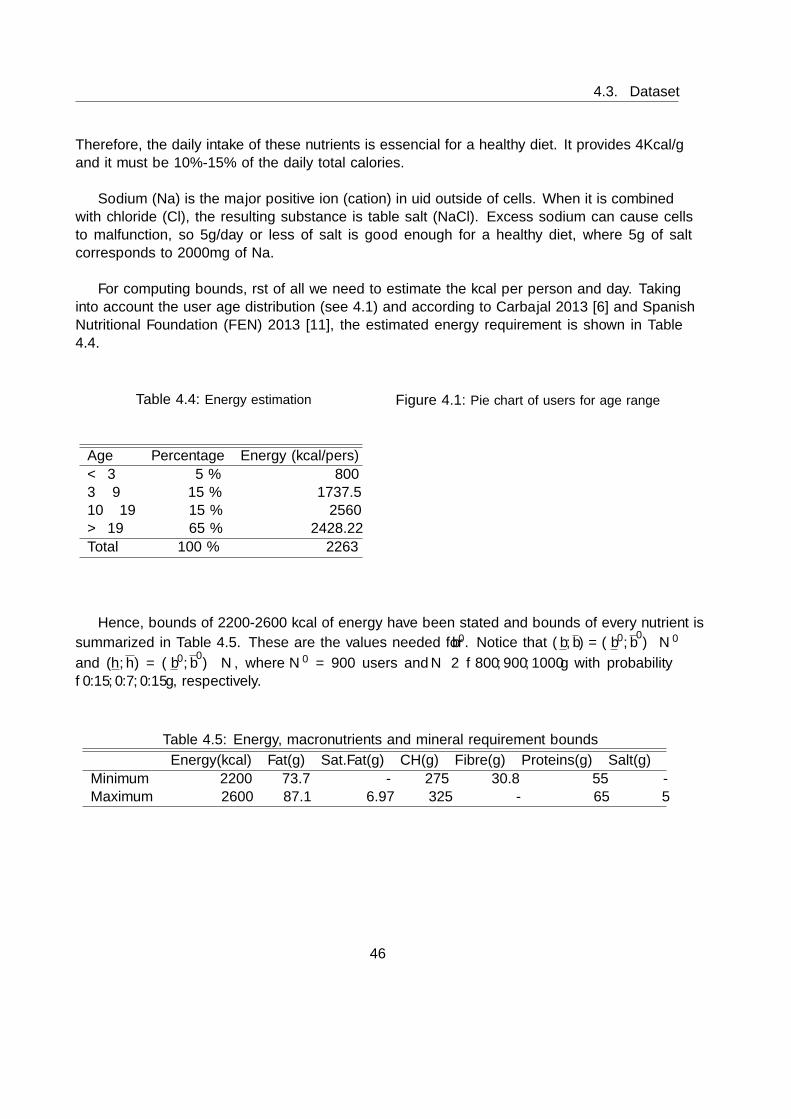
4.3. Dataset
Therefore, the daily intake of these nutrients is essencial for a healthy diet. It provides 4Kcal/gand it must be 10%-15% of the daily total calories.
Sodium (Na) is the major positive ion (cation) in fluid outside of cells. When it is combinedwith chloride (Cl), the resulting substance is table salt (NaCl). Excess sodium can cause cellsto malfunction, so 5g/day or less of salt is good enough for a healthy diet, where 5g of saltcorresponds to 2000mg of Na.
For computing bounds, first of all we need to estimate the kcal per person and day. Takinginto account the user age distribution (see 4.1) and according to Carbajal 2013 [6] and SpanishNutritional Foundation (FEN) 2013 [11], the estimated energy requirement is shown in Table4.4.
Table 4.4: Energy estimation
Age Percentage Energy (kcal/pers)
< 3 5 % 8003− 9 15 % 1737.510− 19 15 % 2560> 19 65 % 2428.22
Total 100 % 2263
Figure 4.1: Pie chart of users for age range
5%
15%
15%
65%
< 33 − 910 − 19> 19
Hence, bounds of 2200-2600 kcal of energy have been stated and bounds of every nutrient is
summarized in Table 4.5. These are the values needed for b0. Notice that (b, b) = (b0, b0) · N0
and (h, h) = (b0, b0) · N , where N0 = 900 users and N ∈ 800, 900, 1000 with probability
0.15, 0.7, 0.15, respectively.
Table 4.5: Energy, macronutrients and mineral requirement bounds
Energy(kcal) Fat(g) Sat.Fat(g) CH(g) Fibre(g) Proteins(g) Salt(g)
Minimum 2200 73.7 - 275 30.8 55 -Maximum 2600 87.1 6.97 325 - 65 5
46
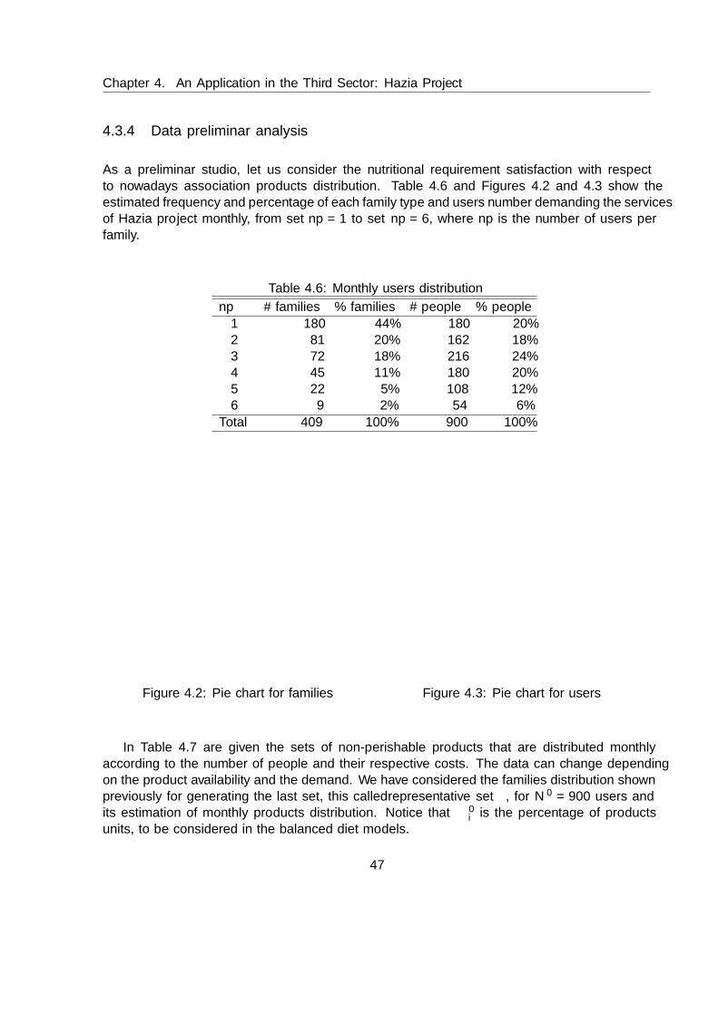
Chapter 4. An Application in the Third Sector: Hazia Project
4.3.4 Data preliminar analysis
As a preliminar studio, let us consider the nutritional requirement satisfaction with respectto nowadays association products distribution. Table 4.6 and Figures 4.2 and 4.3 show theestimated frequency and percentage of each family type and users number demanding the servicesof Hazia project monthly, from set np = 1 to set np = 6, where np is the number of users perfamily.
Table 4.6: Monthly users distribution
np # families % families # people % people
1 180 44% 180 20%2 81 20% 162 18%3 72 18% 216 24%4 45 11% 180 20%5 22 5% 108 12%6 9 2% 54 6%
Total 409 100% 900 100%
44%
20%
18%
11%
5%
2%
Figure 4.2: Pie chart for families
20%
18%
24%
20%
12%
6%
Set1Set2Set3Set4Set5Set6
Figure 4.3: Pie chart for users
In Table 4.7 are given the sets of non-perishable products that are distributed monthlyaccording to the number of people and their respective costs. The data can change dependingon the product availability and the demand. We have considered the families distribution shownpreviously for generating the last set, this called representative set, for N0 = 900 users andits estimation of monthly products distribution. Notice that δ0
i is the percentage of productsunits, to be considered in the balanced diet models.
47

4.3. Dataset
Table 4.7: Monthly set of products for sets of np users
Product Size Price(e)Set Rep. Set %
1 2 3 4 5 6 900 δ0i
Oil 1l 2.85 1 1 2 3 3 4 641 2Pasta 500g 1.03 2 4 5 6 7 9 1546 6Chickpea 1000g 2.89 1 2 3 4 5 6 900 3Maria Biscuits 200g 0.46 2 3 4 5 6 7 1309 5Rice 1000g 2.05 2 2 3 3 3 4 974 4Cacao 1000g 2.09 - - - - - - - -Tuna 80g 0.75 18 36 54 72 90 108 16200 58Sardine 115g 1.85 2 2 3 4 5 6 1080 4Fried Tomato 400g 0.66 3 4 6 8 10 12 1980 7Whole milk 1l 0.95 3 6 9 12 15 18 2700 10Coffee 250g 1.20 1 1 1 1 1 1 409 1
Total 27200e 27738 100%
Consequently, the average of nutrients, per person and day, satisfied by the sets describedpreviously, according to BEDCA, are given in Table 4.8. In Table 4.8 and Figure 4.4 is also shownthe percentages of the minimum nutrients satisfied by the sets defined in Table 4.7 according tothe recommended healthy diet from Table 4.5. Later on, we will compare the nutrients satisfiedby the representative set of 900 people of users and the model proposed in this project.
Table 4.8: Nutrients satisfied per person and day
npEnergy Fat SF CH Fibre Proteins Salt Na
(kcal) (%) (g) (%) (g) (g) (%) (g) (%) (g) (%) (g) (mg)
1 1071 49 58 78 9 114 41 9 29 35 63 1.09 4342 753 34 37 50 6 82 30 8 26 30 55 0.91 3653 776 35 41 56 7 77 28 8 25 29 53 0.90 3624 755 34 43 59 7 68 25 7 24 28 51 0.90 3605 684 31 38 51 7 62 22 7 23 27 50 0.90 3586 716 33 40 54 7 65 24 7 24 28 50 0.90 358
900 812 37 43 59 7 81 29 8 26 30 54 0.94 376
48

Chapter 4. An Application in the Third Sector: Hazia Project
Table 4.9: Satisfied energy, macronutrients and mineral
Energy(%) Fat(%) CH(%) Fibre(%) Proteins(%)
1 49 78 41 29 632 34 50 30 26 553 35 56 28 25 534 34 59 25 24 515 31 51 22 23 506 33 54 24 24 50
900 37 59 29 26 54
Energy Fat CH Fibre Proteins
Set1 Set2 Set3 Set4 Set5 Set6
49
34353431
22
78
505659
5154
41
3028252224292625242324
635553515050
Figure 4.4: Energy, macronutrients and mineral % satisfaction depending on the set
We can observe that the nutritional requirements are not at all satisfied, and specially,proteins satisfaction is poorly guaranteed.
49
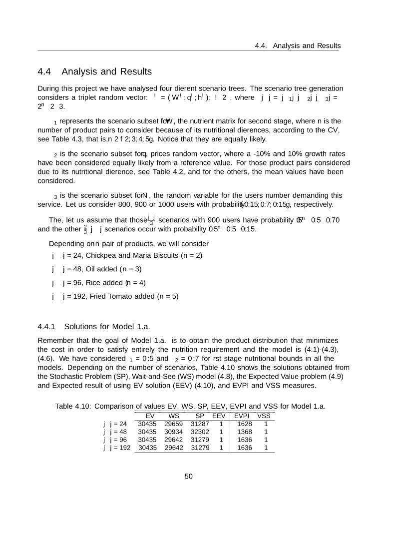
4.4. Analysis and Results
4.4 Analysis and Results
During this project we have analysed four different scenario trees. The scenario tree generationconsiders a triplet random vector: ξω = (Wω, qω, hω), ω ∈ Ω, where |Ω| = |Ω1| · |Ω2| · |Ω3| =2n · 2 · 3.
Ω1 represents the scenario subset for W , the nutrient matrix for second stage, where n is thenumber of product pairs to consider because of its nutritional differences, according to the CV,see Table 4.3, that is, n ∈ 2, 3, 4, 5. Notice that they are equally likely.
Ω2 is the scenario subset for q, prices random vector, where a -10% and 10% growth rateshave been considered equally likely from a reference value. For those product pairs considereddue to its nutritional difference, see Table 4.2, and for the others, the mean values have beenconsidered.
Ω3 is the scenario subset for N , the random variable for the users number demanding thisservice. Let us consider 800, 900 or 1000 users with probability 0.15, 0.7, 0.15, respectively.
The, let us assume that those |Ω|3 scenarios with 900 users have probability 0.5n · 0.5 · 0.70and the other 2
3 · |Ω| scenarios occur with probability 0.5n · 0.5 · 0.15.
Depending on n pair of products, we will consider
• |Ω| = 24, Chickpea and Maria Biscuits (n = 2)
• |Ω| = 48, Oil added (n = 3)
• |Ω| = 96, Rice added (n = 4)
• |Ω| = 192, Fried Tomato added (n = 5)
4.4.1 Solutions for Model 1.a.
Remember that the goal of Model 1.a. is to obtain the product distribution that minimizesthe cost in order to satisfy entirely the nutrition requirement and the model is (4.1)-(4.3),(4.6). We have considered α1 = 0.5 and α2 = 0.7 for first stage nutritional bounds in all themodels. Depending on the number of scenarios, Table 4.10 shows the solutions obtained fromthe Stochastic Problem (SP), Wait-and-See (WS) model (4.8), the Expected Value problem (4.9)and Expected result of using EV solution (EEV) (4.10), and EVPI and VSS measures.
Table 4.10: Comparison of values EV, WS, SP, EEV, EVPI and VSS for Model 1.a.
EV WS SP EEV EVPI VSS|Ω| = 24 30435 29659 31287 ∞ 1628 ∞|Ω| = 48 30435 30934 32302 ∞ 1368 ∞|Ω| = 96 30435 29642 31279 ∞ 1636 ∞|Ω| = 192 30435 29642 31279 ∞ 1636 ∞
50
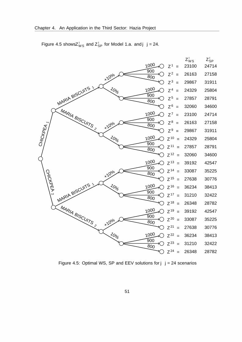
Chapter 4. An Application in the Third Sector: Hazia Project
Figure 4.5 shows ZωWS and ZωSP for Model 1.a. and |Ω| = 24.
Z12 =
Z11 =
Z10 =
Z9 =
Z8 =
Z7 =
Z6 =
Z5 =
Z4 =
Z3 =
Z2 =
Z1 =
Z13 =
Z14 =
Z15 =
Z16 =
Z17 =
Z18 =
Z19 =
Z20 =
Z21 =
Z22 =
Z23 =
Z24 =
ZωWS ZωSP
32060
27857
24329
29867
26163
23100
32060
27857
24329
29867
26163
23100
39192
33087
27638
36234
31210
26348
39192
33087
27638
36234
31210
26348
34600
28791
25804
31911
27158
24714
34600
28791
25804
31911
27158
24714
42547
35225
30776
38413
32422
28782
42547
35225
30776
38413
32422
28782
CH
ICK
PE
A1
CH
ICK
PE
A2
MARIA BISCUITS2
MARIABISCUITS1
MARIABISCUITS1
MARIA BISCUITS2
−10%
+10%
−10%
+10%
+10%
−10%
+10%
−10%
800
9001000
800
9001000
800
9001000
800
9001000
1000
900800
1000
900800
1000
900800
1000
900800
Figure 4.5: Optimal WS, SP and EEV solutions for |Ω| = 24 scenarios
51

4.4. Analysis and Results
Notice that in all the cases it is really worthy to consider uncertainty. EEV is ∞ becausethe solution provided by the Expeted Value is not implementable under all the set of scenarios.Moreover, we can see that the case with more scenarios has higher EVPI. We can also remarkthat with 96 and 192 scenarios, solutions are the same. This happens because the last productbranched, fried tomato, has no relevance.
Table 4.11 reveal the variables X + Y in the best and the worst scenarios accoding to eachmodel (|Ω| = 192), that is, those with minimum and maximum cost, respectively. It expressesthe amount of each product that must be purchased in the initial period of planning horizonand in the middle of planning horizon, according to the brand. Since EEV problem is infeasible,we have omited it from the following tables. Non-displayed products have not been selected.
Table 4.11: Total decisions for Model 1.a.Model 1.a. XEV + YEV Xbest
WS + Y bestWS Xworst
WS + Y worstWS XSP + Y best
SP XSP + Y worstSP
Oil 1057 1051 1219 1018 83Chickpea 6642 5697 5416 - 8448Rice 3642 4471 2814 2227 2102Cacao 3519 2137 5234 4351 -Fried Tomato - - - - 5636
Z (e) 30435e 23003e 39985e 24653e 43999e
The selection of products according to their brands is as follows: for the best scenario in SP,we will choose Oil ’Koipesol’, Chickpeas ’Eroski’, Rice ’La Cigala’ and Fried Tomato ’Eroski’,for the worst, the opposite brands, for the best scenario in WS, it is chosen the same as in SPexcept Oil and for the worst, the same as SP except Fried Tomato.
Figures 4.6 and 4.7 show the histograms obtained for the random variable Z (cost) whereWS and SP models are solved, respectively.
Zws
23000 28000 33000 38000 43000
WS=29642EV=30435SP=31279
Figure 4.6: Histogram of ZWS for Model 1.a.Zsp
23000 28000 33000 38000 43000
WS=29642EV=30435SP=31279
Figure 4.7: Histogram of ZSP for Model 1.a.
Notice that means of the variable cost, Z, according to each problem WS, SP and EV, areexpressed by the vertical lines.
52
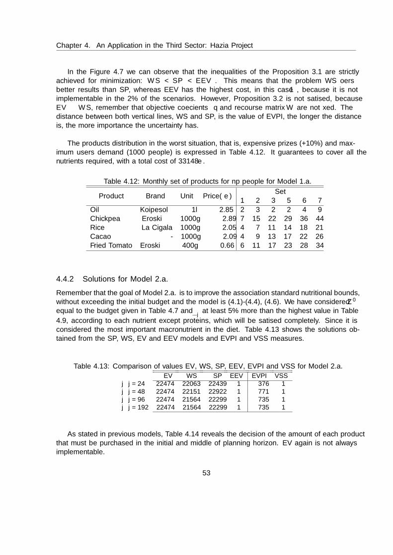
Chapter 4. An Application in the Third Sector: Hazia Project
In the Figure 4.7 we can observe that the inequalities of the Proposition 3.1 are strictlyachieved for minimization: WS < SP < EEV . This means that the problem WS offersbetter results than SP, whereas EEV has the highest cost, in this case ∞, because it is notimplementable in the 2% of the scenarios. However, Proposition 3.2 is not satisfied, becauseEV WS, remember that objective coefficients q and recourse matrix W are not fixed. Thedistance between both vertical lines, WS and SP, is the value of EVPI, the longer the distanceis, the more importance the uncertainty has.
The products distribution in the worst situation, that is, expensive prizes (+10%) and max-imum users demand (1000 people) is expressed in Table 4.12. It guarantees to cover all thenutrients required, with a total cost of 33148e.
Table 4.12: Monthly set of products for np people for Model 1.a.
Product Brand Unit Price(e)Set
1 2 3 5 6 7
Oil Koipesol 1l 2.85 2 3 2 2 4 9Chickpea Eroski 1000g 2.89 7 15 22 29 36 44Rice La Cigala 1000g 2.05 4 7 11 14 18 21Cacao - 1000g 2.09 4 9 13 17 22 26Fried Tomato Eroski 400g 0.66 6 11 17 23 28 34
4.4.2 Solutions for Model 2.a.
Remember that the goal of Model 2.a. is to improve the association standard nutritional bounds,without exceeding the initial budget and the model is (4.1)-(4.4), (4.6). We have considered Z0
equal to the budget given in Table 4.7 and βj
at least 5% more than the highest value in Table
4.9, according to each nutrient except proteins, which will be satisfied completely. Since it isconsidered the most important macronutrient in the diet. Table 4.13 shows the solutions ob-tained from the SP, WS, EV and EEV models and EVPI and VSS measures.
Table 4.13: Comparison of values EV, WS, SP, EEV, EVPI and VSS for Model 2.a.
EV WS SP EEV EVPI VSS|Ω| = 24 22474 22063 22439 ∞ 376 ∞|Ω| = 48 22474 22151 22922 ∞ 771 ∞|Ω| = 96 22474 21564 22299 ∞ 735 ∞|Ω| = 192 22474 21564 22299 ∞ 735 ∞
As stated in previous models, Table 4.14 reveals the decision of the amount of each productthat must be purchased in the initial and middle of planning horizon. EV again is not alwaysimplementable.
53

4.4. Analysis and Results
Table 4.14: Total decisions for Model 2.a.Model 2.a. XEV + YEV Xbest
WS + Y bestWS Xworst
WS + Y worstWS XSP + Y best
SP XSP + Y worstSP
Oil 1165 994 1053 1177 959Pasta 16052 16565 12669 16160 23419Chickpea 1849 1396 4205 1598 1909Rice 2320 1422 3564 842 842
Z 22474 17384 27129 18322 27185
In Model 2.a. the best scenarios follow the same steps as the best scenario in SP for Model1.a., and the worst, the same as the worst scenario in WS for Model 1.a.
The nutrients satisfaction by the representative set of 900 users of Sortarazi compared withthe one created by this Model 2.a. is shown in Figure 4.8.
Energy CH Fibre Proteins% o
f the
min
imum
req
uire
men
t sat
isfie
d
Model SP2Sortarazi
89%
37%
110%
29%
103%
26%
100%
54%
Figure 4.8: Comparison of nutrients requirement satisfaction for Model 2.a.
Since nutrients satisfaction have improved, the new recommendation of products supplymentis shown in Table 4.15, with a total cost of 23276e, even smaller than the initial budget.
Table 4.15: Monthly set of products for np people for Model 2.a.
Product Brand Unit Price(e)Set
1 2 3 4 5 6
Oil Koipesol 1l 2.85 1 3 4 6 7 8Pasta - 500g 1.03 16 32 48 65 81 97Chickpea Eroski 1000g 2.89 2 4 6 9 11 13Rice La Cigala 1000g 2.05 3 6 9 12 15 19
54

Chapter 4. An Application in the Third Sector: Hazia Project
4.4.3 Solutions for Model 1.b.
Remember that the goal of Model 1.b. is to obtain the product distribution that minimizesthe cost and mantains a balanced diet satisfying all the nutrition requirement and the modelis (4.1)-(4.6). Although Models 1.a. and 2.a. reach our goals, we have realized that the newproduct distribution would not imply a balanced diet, but the minimum cost for the nutritionalbounds fixed. So, we have decided to create another two models, with the same goals as before,but adding two new constraints (4.5) and (4.6), where δi = 0.15 · δ0
i for X and δ′i = 0.10 · δ0i
for Y ω. δ0i is the percentage of each product and it is shown in Table 4.7. Notice that we have
chosen 0.15 and 0.10 in order to mantain feasibility.
For the sake of simplification, we are going to show only the analysis of all the problems forthe biggest scenario set, |Ω| = 192, in the balanced models. Table 4.16 summarizes the optimalobjective function for SP, WS, EV and EEV, and EVPI and VSS measures.
Table 4.16: Comparison of values EV, WS, SP, EEV, EVPI and VSS for Model 1.b.
EV WS SP EEV EVPI VSS|Ω| = 192 36021 34542 36930 ∞ 2389 ∞
The total amount of products, that must be provided in the best and worst situations, isgiven in Table 4.17. Since some ZEEV problems are infeasible, we have omited EEV from thesolutions.
Table 4.17: Best and worst cases depending on the problem for Model 1.b.
Model 1.b. XEV + YEV XbestWS + Y best
WS XworstWS + Y worst
WS XSP + Y bestSP XSP + Y worst
SP
Oil 949 870 1024 885 875Pasta 332 286 281 269 322Chickpea 5786 7133 7080 5184 6859Maria Biscuits 112 81 78 70 105Rice 1166 1334 1633 784 1837Cacao 6047 4960 6376 5748 5757Tune 1625 417 1129 1008 1523Sardine 112 81 78 70 105Fried Tomato 1638 142 4325 4289 16883Whole Milk 280 203 195 174 263Coffe 28 89 19 17 26
Z(e) 36021e 26981e 53709e 29802e 52207e
The selection of products according to their brands follows the same steps as Models 1.a.and 2.a., except for Fried Tomato, that it is always chosen the first brand.
Finally, the new recommendation of products supplyment in the worst situation is shown inTable 4.18, with a total cost of 41641e.
55

4.4. Analysis and Results
Table 4.18: Monthly set of products for np people for Model 1.b.
Product Brand Unit Price(e)Set
1 2 3 4 5 6
Oil Koipesol 1l 2.85 1 2 3 4 4 5Pasta - 500g 1.03 - 1 1 1 2 2Chickpea Eroski 1000g 2.89 7 14 21 27 34 41Maria Biscuits Gullon 200g 0.46 - - - - 1 1Rice La Cigala 1000g 2.05 2 4 6 7 9 11Cacao - 1000g 2.09 6 12 17 23 29 35Tuna - 80g 0.75 2 3 5 6 8 9Sardine - 115g 1.85 - - - - 1 1Fried Tomato Eroski 390g 0.66 17 34 51 68 84 101Whole milk - 1l 0.95 - 1 1 1 1 2
4.4.4 Solutions for Model 2.b.
Once again, we will compare all the situations according to the biggest number of scenarios forModel 2.b., considering that the budget is 27200e.
In Table 4.19 is given the optimal objective function for each problem: SP, WS, EV andEEV and EVPI and VSS measures.
Table 4.19: Comparison of values EV, WS, SP, EEV, EVPI and VSS for Model 2.b.
EV WS SP EEV EVPI VSS|Ω| = 192 23305 22760 22998 ∞ 239 ∞
The total amount of products, that must be provided in the best and worst situations, isgiven in Table 4.20. Since some ZEEV problems are infeasible, we have omited EEV from thesolutions.
Table 4.20: Best and worst cases depending on the problem for Model 2.b.
Model 2.b. XEV + YEV XbestWS + Y best
WS XworstWS + Y worst
WS XSP + Y bestSP XSP + Y worst
SP
Oil 58 678 58 542 83Pasta 17884 15530 16930 15506 19295Chickpea 951 1505 1803 1356 1118Maria Biscuits 8974 144 12468 1875 10718Rice 115 115 331 122 167Cacao 29 29 29 36 42Tune 1675 1675 1675 1778 2420Sardine 115 115 115 123 167Fried Tomato 202 202 202 215 292Whole Milk 289 289 289 307 417Coffe 29 29 29 31 42
Z(e) 21555e 18353e 24952e 18542e 27076e
56
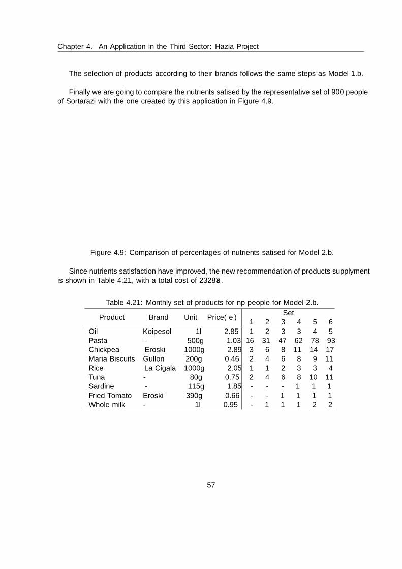
Chapter 4. An Application in the Third Sector: Hazia Project
The selection of products according to their brands follows the same steps as Model 1.b.
Finally we are going to compare the nutrients satisfied by the representative set of 900 peopleof Sortarazi with the one created by this application in Figure 4.9.
Energy CH Fibre Proteins% o
f the
min
imum
req
uire
men
t sat
isfie
d
Model SP4Sortarazi
74%
37%
83%
29%
110%
26%
95%
54%
Figure 4.9: Comparison of percentages of nutrients satisfied for Model 2.b.
Since nutrients satisfaction have improved, the new recommendation of products supplymentis shown in Table 4.21, with a total cost of 23283e.
Table 4.21: Monthly set of products for np people for Model 2.b.
Product Brand Unit Price(e)Set
1 2 3 4 5 6
Oil Koipesol 1l 2.85 1 2 3 3 4 5Pasta - 500g 1.03 16 31 47 62 78 93Chickpea Eroski 1000g 2.89 3 6 8 11 14 17Maria Biscuits Gullon 200g 0.46 2 4 6 8 9 11Rice La Cigala 1000g 2.05 1 1 2 3 3 4Tuna - 80g 0.75 2 4 6 8 10 11Sardine - 115g 1.85 - - - 1 1 1Fried Tomato Eroski 390g 0.66 - - 1 1 1 1Whole milk - 1l 0.95 - 1 1 1 2 2
57
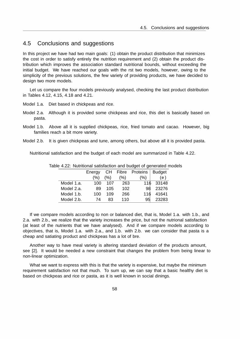
4.5. Conclusions and suggestions
4.5 Conclusions and suggestions
In this project we have had two main goals: (1) obtain the product distribution that minimizesthe cost in order to satisfy entirely the nutrition requirement and (2) obtain the product dis-tribution which improves the association standard nutritional bounds, without exceeding theinitial budget. We have reached our goals with the first two models, however, owing to thesimplicity of the previous solutions, the few variety of providing products, we have decided todesign two more models.
Let us compare the four models previously analysed, checking the last product distributionin Tables 4.12, 4.15, 4.18 and 4.21.
Model 1.a. Diet based in chickpeas and rice.
Model 2.a. Although it is provided some chickpeas and rice, this diet is basically based onpasta.
Model 1.b. Above all it is supplied chickpeas, rice, fried tomato and cacao. However, bigfamilies reach a bit more variety.
Model 2.b. It is given chickpeas and tune, among others, but above all it is provided pasta.
Nutritional satisfaction and the budget of each model are summarized in Table 4.22.
Table 4.22: Nutritional satisfaction and budget of generated models
Energy CH Fibre Proteins Budget(%) (%) (%) (%) (e)
Model 1.a. 100 107 263 116 33148Model 2.a. 89 105 102 98 23276Model 1.b. 100 109 266 116 41641Model 2.b. 74 83 110 95 23283
If we compare models according to non or balanced diet, that is, Model 1.a. with 1.b., and2.a. with 2.b., we realize that the variety increases the price, but not the nutrional satisfaction(at least of the nutrients that we have analysed). And if we compare models according toobjectives, that is, Model 1.a. with 2.a., and 1.b. with 2.b. we can consider that pasta is acheap and satiating product and chickpeas has a lot of fibre.
Another way to have meal variety is altering standard deviation of the products amount,see [2]. It would be needed a new constraint that changes the problem from being linear tonon-linear optimization.
What we want to express with this is that the variety is expensive, but maybe the minimumrequirement satisfaction not that much. To sum up, we can say that a basic healthy diet isbased on chickpeas and rice or pasta, as it is well known in social dinings.
58
Chapter 5
Conclusions
In this report basic concepts of the Stochastic Optimization have been studied. This disciplinebelongs to the Applied Mathematical area of Operations Research and Management Science,and deals with mathematical models under uncertainty.
First of all, we have defined and compared deterministic and stochastic programming inorder to show the relevance of the latter. It is known that most of the Optimization problemsin the real life present uncertain data and this is why Stochastic Programming is an alternativeto model them. This project is focused in two-stage Stochastic Programming, where first stagedecisions must be taken here-and-now, before uncertainty is revealed, and second stage-onesafter it, providing decisions for the set of scenarios. There are explained some basic propertiessuch as probability spaces and random variables, decisions and recourses and non-anticipativityprinciple. Stochastic Problems, satisfy explicitly or implicitly this principle, that is, there is aunique first-stage decision vector, X, whereas there are |Ω| second-stage decisions, Y ω, one foreach scenario. The problem is feasible for each scenario and X is optimal over all scenarios,since all the first stage decisions are made simultaneously.
Appart from the two-stage Stochastic Problem, some other alternative models are described.Wait-and-See model, WS, is an approximation based on the perfect information and it is equiv-alent to the SP relaxing anticipativity principle. It is also defined the Expected Value problem,EV, a simplification by the replace of all random variables with the expected value. If we fixthe optimal solution of the first-stage in SP, the Expected result of using Expected Value, EEVis reached.
We have designed expressly a diet problem example in three different stochasticity cases inorder to explain all the theorical models exposed and compare them. We have realized that it isnot easy to get explanatory solutions with a simplified problem. In other words, the examplesgiven in the literature books can contain painstakingly selected data.
According to the introduced models, two measures have been defined: the expected value ofperfect information (EVPI) and the value of stochastic solutions (VSS). EVPI is the maximumprice that the decision maker should pay in order to know the uncertainty in advance and it isdefined as the difference between WS and SP, whereas VSS is the real cost of ignoring it and it is
59

defined as the difference between EEV and SP. Based on these measures, we have concluded thatsometimes is worthwhile to calculate the stochastic solution, but we cannot know it previously.Main inequalities of the measures have been verified. Proposition 3.1, WS ≤ SP ≤ EEV hasbeen checked with the three cases of the diet example, metioned before. The third case is theonly one that fulfills the inequality of the Proposition 3.2, EV ≤ WS, because recourse matrixand objective coefficients are fixed. Therefore, we can confirm that it is absolutely inadecuate totrust on the solution of the expected value problem, EV, since it is expected a better value thanthe one under perfect information, WS. We have also studied some relations between EVPI andVSS. As it can be seen in the definition, EVPI and VSS will never be negative, see Proposition3.3. If we verify Proposition 3.4, EV PI ≤ EEV − EV and V SS ≤ EEV − EV , for the threecases, as we expected, the third one is the unique that satisfies it.
After theory explanation, a real problem application has been considered. Motivated onthe malnutrition, poverty and wasted food all around the world, Spain included, we realizedthat it would be interesting to apply maths in the third sector, also known as social economy.In particular, to optimize the food distribution in a local Food Bank, managed by a nonprofitorganization. We have modeled a two-stage stochastic Diet Problem with 24, 48, 96 and 192scenarios. A general model have been described with two different goals: (1) obtain the productdistribution that minimizes the cost in order to satisfy entirely the nutrition requirement, withor without balanced diet and (2) improve the association standard nutritional bounds, withoutexceeding the initial budget and with or without balanced diet. Once data from the foodstorehouse was taken, we have decided which pair of products are nutritionally more differentin order to create the scenario tree. In all the cases solutions provided by the expected valueproblem have been infeasible in some of the scenarios. Therefore they get the worst cost, that is,provided decisions are not implementable. This means that in all the cases it is really worthy toconsider uncertainty. Since reporting 192 different decisions obtained for each model, SP, WS,EV and EEV would be too long, the best and the worst solutions of both models have beenshown. After that, the food distributions depending on families have been summarized. Thedifference of the nutritional requirement satisfied, between their product sets and our results areremarkable. The optimal solutions provide few meal variation. After, the solutions of the fourmodels have been compared. As it is well known in hostels, canteens or social restaurants, ricewith legumes is a full nutritional meal. It is logical that the results depends on the goal. For abalanced diet, also a constraint with standard deviation bounded could be added, see [2], butthe linear problem would change to a quadratic one. A varied set of products increase quite alot the cost.
To conclude, we would like to remark that we just have given some suggestions thanks to thissimplified application results analysis, considering some of the nutrients needed in a healthy diet.However, from now on, this application will be given over to specialists: nutricionists, healthprofessional, social services and the people in charge of association, among others; obviously, inorder to help in the decision making, since they have the final say.
60
Appendix A
GAMS CODE: Examples
The GAMS codes of examples in Chapters 2 and 3, for Cases 1, 2 and 3, can be downloadedfrom https://ehubox.ehu.eus/index.php/s/8LP7rmcqvb5w1T3.
The code of the program examples.gms obtains the solutions of the deterministic problem(2.2) and SP problem (2.4)-(2.7) in Chapter 2, and WS (3.2), EV (3.6) and EEV (3.11) modelsof the examples in Chapter 3. Moreover, EVPI (3.15) and VSS (3.16) measures are computed.
61

62

Appendix B
GAMS CODE: Application in thethird sector
The GAMS codes of Model 1.a. for |Ω| = 192 in Chapter 4 can be download from the linkhttps://ehubox.ehu.eus/index.php/s/hvljPEjbhibANAl.
The code of the program application.gms obtains the solutions of the SP problem (4.1)-(4.6)in Chapter 4, and WS (4.8), EV (4.9) and EEV (4.10) models of the application of Model 1.a.for |Ω| = 192 in Chapter 4. Moreover, EVPI and VSS measures are computed.
63

64
Bibliography
[1] A. Alonso-Ayuso, L.F. Escudero, A. Garın, M.T. Ortuo & G. Perez. On the product selection and plant dimensioningunder uncertainty. Omega, 33:307-318, 2005.
[2] Prof. Armbruster, F. Ferrero, E. Hsieh & A. Wagner. Diet Optimization Problem. IEMS 310 Spring, 2009.
[3] E. M. L. Beale. On minimizing a convex function subject to linear inequalities. Journal of the Royal Statistical Society.Series B (Methodological), 173184, 1955.
[4] J. R. Birge. Stochastic Programming Computation and Applications. Journal of Computing, 9(2):111-133, 1997.
[5] J. R. Birge and F. Louveaux. Introduction to Stochastic Programming. Springer Science & Business Media, 2011.
[6] A. Carbajal Azcona. ”Ingestas recomendadas de energıa y nutrientes” en: M. T. Garcıa-Arias & M. C. Garcıa-Fernandez, Eds., Nutricion y dietetica, 2:27-44, 2003. Updated in 2013.
[7] Y. Censor & S. A. Zenios. Parallel Optimization. Theory, Algorithms and Applications. Oxford University Press,1997.
[8] G. B. Dantzig. Linear programming under uncertainty. Management science, 1(3-4):197206, 1955.
[9] L. F. Escudero, A. Garın, M. Merino & G. Perez. The Value of the Stochastic Solution in Multistage Problems.Sociedad de Estadstica e Investigacin Operativa, 15:48-64, 2007.
[10] A. Ferguson & G.B. Dantzig. The allocation of aircraft to routes: an example of linear programming under uncertaindemands, Management Science, 3:45-73, 1956.
[11] Fundacion Espanola de la Nutricion (FEN). Libro Blanco de la Nutricion en Espana, 2013.
[12] H.I. Gassman & W.T. Ziemba. Stochastic Programming: applications in finance, energy, planning and logistics.World Scientific, 2012.
[13] M. Gjerris & S. Gaiani. ’Values in the trash: ethical aspects of food waste’ in: L. Escajedo San-Epifanio & M. DeRenobales Scheifler, Eds., Envisioning a future without food waste and food poverty, 1:23-31, 2015.
[14] L. Gonzalez Vaque. ’Food loss and waste: some short- and medium-term proposal for the European Union’ in: L.Escajedo San-Epifanio & M. De Renobales Scheifler, Eds., Envisioning a future without food waste and food poverty,1:23-31, 2015.
[15] S. C. Graves & W. C. Jordan. Principles of the Benefits of Manufacturing Process Flexibility, General MotorsLaboratories Research Publication, 1991.
[16] J. L. W. V. Jensen. Sur les fonctions convexes et les ingalits entre les valeurs moyennes. Acta Mathematica,30(1):175193, 1906.
[17] P. Kall, A. Ruszczynski & K. Frauendorfer. Approximation techniques in stochastic programming. Numerical tech-niques for stochastic optimization, 3364, 1988.
[18] P. Kall & S.W. Wallace. Stochastic Programming. John Wiley, 1994.
65

Bibliography
[19] E. Kao & M. Queyranne. Budgeting costs of nursing in a hospital, Management Science 31:373-395, 1985.
[20] A. King. ”Stochastic programming problems: Examples from the literature” in: Y.Ermoliev & R. West, Eds., Nu-merical Techniques for Stochastic Optimization (Springer-Verlag, Berlin), 543-567, 1988.
[21] A. J. King & S. W. Wallace. Modeling with Stochastic Programming. Springer Series in Operations Research andFinancial Engineering, 2012.
[22] W.K. Klein Haneveld & M.H. van der Vlerk. Optimizing electricity distribution using two-stage integer recousemodels. In S. Uryasev & P.M Pardalos, editors. Stochastic Optimization: Algorithms and Applications, KluwerAcademic Publisher, 137-154, 2001.
[23] A. Madansky. Inequalities for stochastic linear programming problems. Management science, 6(2):197-204, 1960.
[24] J. M. Mulvey, R. J. Vanderbei & S. A. Zenios. Robust Optimization of Large-Scale Systems, Operations Research,2:264-281, 1995.
[25] A. Prekopa. Stochastic Programming. Kluwer Academic Publishers, Dordrecht, 1995.
[26] R. T. Rockafellar & R. J. B. Wets. Non-anticipativity and L′-Martingales in Stochastic Optimization Problems,Stochastic Systems: Modeling, Identification, and Optimization, Math. Programming Study, 6:170-187, 1976.
[27] R. T. Rockafellar & R. J-B Wets. Scenario and policy aggregation in optimization under uncertainty. Mathematics ofOperations Research, 16:119-147, 1991.
[28] R. Schlaifer and H. Raiffa. Applied statistical decision theory (Harvard University, Boston, MA, 1961).
[29] A. Shapiro, D. Dentcheva & A. Ruszczynski. Lectures on stochastic programming: Modeling and theory. MPS-SIAMBook Series on Optimization 9, 2009.
[30] G. J. Stigler. The cost of the subsistence. Journal of farm economics, 27(2):303-314, 1945.
[31] W. Swart, C. Smith, & T. Holderby. ”Expansion Planning for a Large Dairy Farm,” Chapter 8 in Studies in LinearProgramming, H. Salkin and J. Saha, eds. North Holland, Amsterdam, 1975.
[32] B. Vitoriano, J. Montero de Juan & D. Ruan. Decisions aid models for disaster management and emergency. AtlantisPress, 2013.
[33] S.W. Wallace & W.T. Ziemba, editors. Applications of Stochastic Programming: MPS-SIAM Book Series in Opti-mization, 2005.
[34] R. J-B Wets. Stochastic programs with fixed recourse: the equivalent deterministic problem. SIAM Review, 16:309-339, 1974 .
[35] NEOS Server. Diet Problem: http://www.neos-guide.org/content/diet-problem
[36] BEDCA - Base espanola de composicion de alimentos: http://www.bedca.net
[37] Hirugarren sektoreko Sortarazi elkartearen web orria: http://www.sortarazi.org/
[38] Shopping in EROSKI online: https://www.compraonline.grupoeroski.com/
[39] Eustat - Euskal Estatistika Erakundea - Instituto Vasco de Estadıstica: http://www.eustat.eus/
[40] SPS - Stochastic Programming Society: http://stoprog.org
[41] GAMS modeling system for mathematical programming and optimization: https://www.gams.com/
[42] R-project software for statistical computing and graphics: https://www.r-project.org/
[43] IBM ILOG CPLEX Optimizer: http://www-01.ibm.com/software/integration/optimization/cplex-optimizer/
66