twri 3-c2 - part 3 - usgs

WSGS science for a changing world

Techniques of Water-Resources Investigations of the U.S. Geological Survey

Book 3, Applications of Hydraulics

Chapter C2

Field Methods for Measurement of Fluvial Sediment

By Thomas K. Edwards and G. Douglas Glysson

This manual is a revision of “Field Methods for Measurement of Fluvial Sediment,” by Harold I? Guy and Vernon W. Norman, U.S. Geological Survey Techniques of Water-Resources Investigations,‘Book 3, Chapter C2, published in 1970.

http://www.usgs.gov

reidell

Click here to return to USGS Publications

../index.html

38 FIELD METHODS FOR MEASUREMENT OF FLUVIAL SEDIMENT

station. Stream depth determines whether hand samplers, such as the DH-48 or the BMH-53, or cable- suspended samplers, such as the D-74 or the P-61, should be used. Depths over 15 feet will require the use of point samplers as depth-integrating samplers to avoid overfilling or using too fast a transit rate. Stream velocity as well as depth are factors in determining whether or not a stream can be waded. A general rule is that when the product of depth in feet and velocity in feet per second equals 10 or greater, a stream’s wadability is questionable. Application of this rule will vary considerably among field persons according to an individual’s stature and the condition of the streambed. That is, if footing is good on the streambed, a heavier field person with a stocky build will generally wade more easily than will a lighter, thinner person when a stream depth-velocity product approaching 10 exists.

The depth-velocity product also affects the action of each sampler. The larger this product, the heavier and more stable the sampler must be to collect a good sample. At a new station or for inexperienced persons, considerable trial and error may be necessary to determine which sampler is best for a given stream condition.

All sampler nozzles, gaskets, and air exhausts, as well as the other necessary equipment, should be checked regularly and replaced or serviced if necessary. Sampler nozzles in particular should be checked to ensure that they are placed in the appropriate instrument or series. See the guidelines presented in table 1 to determine whether the nozzle is correct. The correct size of nozzle. to use for a given situation must often be determined by trial. As mentioned in the previous section, it is best to use the largest nozzle possible that will permit depth integration without overtilling the sample bottle or exceeding the maximum transit rate (about 0.4 of the mean velocity in the sampled vertical for most samplers with pint containers).

If a sample bottle does not fill in the expected time, the nozzle or air-exhaust passages may be partly blocked. The flow system can be checked, as described in the section titled “Gaskets,” by sliding a length of clean rubber or plastic tubing over the nozzle and blowing through the nozzle with a bottle in the sampler. This procedure should be performed carefully, avoiding direct contact with the nozzle, thus eliminating the possibility of ingesting any pollutant that might exist on the sampler. When air pressure is

applied in this manner, circulation will occur freely through the nozzle, sample container, and out the air exhaust. Obstructions can be cleared by removing and cleaning the nozzle and (or) air exhaust, using a flexible piece of multistrand wire. This procedure should be adequate for most airway obstruction problems. However, if blockage results from accumu- lation of ice or from damage to the sampler, a heat source must be used to melt the ice or the sampler must be sent to the F.I.S.P. or HIF repair facility. Point samplers can be checked using the same technique, if the valve mechanism is placed in the sampling position while air is forced into the nozzle and through the air exhaust.

All support equipment required for sampling, such as cranes, waders, taglines, power sources, and current meters, should be examined periodically, and as used, to ensure an effective and safe working condition. For example, be certain that the supporting cable to the sampler or current meter is fastened securely in the connector; if worn or frayed places are noted, the cable should be replaced. Power equipment used with the heavier samplers and point samplers need a periodic operational check and battery charge. Point samplers should be checked immediately before use to determine, among other things, if the valve is opening and closing properly. By exercising such precautions, the field person will avoid unnecessary exposure to traffic on the bridge and will avoid lost sampling time should repairs and adjustments be required.

Maintenance of samplers and support equipment will be facilitated if a file of instructions for assembly, operation, and maintenance of equipment can be accumulated in the field office. Such a file could include F.I.S.P. reports as well as other pertinent information available from HIP.

Suspended-Sediment Sampling Methods

Sediment-Discharge Measurements

The usual purpose of sediment sampling is to determine the instantaneous mean discharge-weighted suspended-sediment concentration at a cross section. Such concentrations are combined with water discharge to compute the measured suspended- sediment discharge. A mean discharge-weighted suspended-sediment concentration for the entire cross

SEDIMENT-SAMPLJNG TECHNIQUES 39

section is desired for this purpose and for the develop- ment of coefficients to adjust observer and automatic pumping-type sampler data.

Ideally, the best procedure for sampling any stream to determine the sediment discharge would be to collect the entire flow of the stream over a given time period, remove the water, and weigh the sediment. Obviously, this method is a physical impossibility in the majority of instances. Instead, the sediment concentration of the flow is determined by (1) collecting depth-integrated suspended-sediment samples that define the mean discharge-weighted concentration in the sample vertical and (2) collecting sufficient verticals to define the mean discharge- weighted concentration in the cross section.

Single Vertical

The objective of collecting a single-vertical sample is to obtain a sample that represents the mean discharge-weighted suspended-sediment concentration in the vertical being sampled at the time the sample was collected. The method used to do this depends on the flow conditions and particle size of the suspended sediment being transported. These conditions can be generalized to four types of situations: (1) low velocity (~2.0 ft/s) when little or no sand is being transported in suspension; (2) high velocity (2.o<v<12.0 ft/s) when depths are less than 15 feet; (3) high velocity (2.O<v<12.0 ft/s) when depths are greater than 15 feet; and (4) very high velocities (v>12.0 ft/s).

First case.-In the first case, the velocity is low enough that no sand is being transported as suspended sediment. The distribution of sediment (silt and clay) is relatively uniform from the stream surface to bed (Guy, 1970, p. 15). The sampling error for this case, when only sediment particles less than 0.062 mm are in suspension, is small, even with intake velocities somewhat higher or lower than the ambient mean stream velocities. Therefore, it is not as important to collect the sample isokinetically with fines in suspension as it is when particles greater than 0.062 mm are in suspension. In shallow streams, a sample may be collected by submerging an open-mouthed bottle into the stream by hand. The mouth should be pointed upstream and the bottle held at approximately a 45degree angle from the streambed. The bottle should be filled by moving it from the surface to the streambed and back. Care should be taken to avoid

touching the mouth of the bottle to the streambed. An unsampled zone of about 3 inches should be maintained in order to obtain samples that are compat- ible with depth-integrated samples collected at higher velocities.

If the stream is not wadable, a weighted-bottle type sampler may be used. Remember that these samples are not discharge-weighted samples and that, if possible, their analytical results should be verified by or compared to data obtained using a standard sampler and sampling technique.

Second case.-In the second case, when 2Lkvc12.0 ft/s and the depth is less than 15 feet, the standard depth-integrating samplers, such as‘ DH-48, DH-75, DH-59, D-49, and D-74 may be used. The method of sample collection is basically the same for all these samplers, whether used while wading or from a bridge or cableway. Insert a clean sample bottle into the sampler and check to see that there are no obstructions in the nozzle or air-exhaust tube. Then lower the sampler to the water surface so that the nozzle is above the water, and the lower tail vane or back of the sampler is in the water for proper upstream- downstream orientation. After orientation of the sampler, depth integration is accomplished by traversing the full depth and returning to the surface with the sampler at a constant transit rate.

When the bottom of the sampler touches the streambed, immediately reverse the sampler direction and raise the sampler to clear the surface of the flow at a constant transit rate. The transit rate used in raising the sampler need not be the same as the one used in lowering, but both rates must be constant in order to obtain a velocity- or discharge-weighted sample. The rates should be such that the bottle fills to near its optimum level (approximately 3 inches below the top or 350 to 420 milliliters, for the pint milk bottle, or 2 inches below the top or 650 to 800 milliliters for the quart bottle).

For streams that transport heavy loads of sand, and perhaps for some other streams, at least two complete depth integrations of the sample vertical should be made as close together in time as possible, one bottle for each integration. Each bottle then constitutes a sample and can be analyzed separately or, for the purposes of computing the sediment record, concentrations from two or more bottles can be averaged, whereby they are called a set. This set then is a sample in time with respect to the record. Sample analyses from two or more individual bottles for a given

40 FIELD METHODS FOR MEASUREMENT OF FLUVJAL SEDIMENT

observation are useful for checking sediment variations among bottles-an obvious advantage in the event the sediment concentration in one bottle is quite different from the concentration in the other bottles for the same observation. Immediately after collection, every bottle or sample should be inspected visually by swirling the water in the bottle and observing the quantity of sand particles collected at the bottom. If there is an unusually large quantity or a difference in the quantity of sands between bottles, another sample from the same vertical should be taken immediately. The sample suspected of having too much sand should be discarded. If it is saved, an explanation such as “too much sand” should be clearly written on the bottle. If by chance, a bottle is overfilled or if a spurt of water is seen coming out of the nozzle when the sampler is

raised past the water surface, the sample should be discarded. A clean bottle must be used to resample the vertical.

To help avoid the problem of striking the nozzle into a dune or settling the sampler too deeply into a soft bed, it is recommended that a slow downward integration be used, followed by a more rapid upward integration. Because most of the sand is transported near the bed, it is essential that the transit direction of the sampler be immediately reversed as the sampler touches the bed.

Pertinent information as shown in figure 27 must be available with each bottle for use in the laboratory and in compiling the record. Most districts provide bottles with an etched area on which a medium-soft lead (blue or black) or wax pencil can be used. Other districts use

If water exceeds this level 46car4 sample an4 obtam another m a clean bottle (applicable to all sampling methods)

>

Dewed range for water level for smgle vertical samples

- Etched wtmg area

If water IS less than this level. Integrate agam - usmg vans0 rate at least as fast as first time

(applicable to SWI method when composltlng multlple verticals m a bottle durmg samplmg)

Mark with a soft blue or black pencil

Figure 27. Sample bottle showing desired water levels for sampling methods indicated and essential record information applicable to all sampling methods.

SEDIMENT-SAMPLING TECHNIQUES 41

plain bottles and attach tags for recording the required information. The required information may be recorded on the bottle cap if there are no other alterna- tives, but this should be avoided because of the small writing space and because of the possibility of putting the cap on the wrong bottle. Paper caps should not be used because they do not form as good a seal as do the plastic caps and may allow evaporation of the sample.

Third case.-In the third case, the depth-integrating samplers cannot be used because the depth exceeds the maximum allowable depth for these samplers. In this case, one of the point-integrating or bag-type samplers must be used. Because the bag sampler is still new and sufficient field data have not been collected to verify its sampling efficiency, USGS personnel who wish to use it must contact the Chief, Office of Surface Water, Reston, Virginia, and must set up a comparability sampling system to verify the sampler’s efficiency under their specific conditions. The technique for collection of a sample using the bag-type sampler is similar to that used with the depth-integrating samplers.

The point samplers may be used to collect depth- integrated samples in verticals where the depth is greater than 15 feet. For streams with depths between 15 and 30 feet, the procedure is as follows: 1. Insert a clean bottle in the sampler and close the

sampler head. 2. Lower the sampler to the streambed, keeping the

solenoid closed and note the depth to the bed. 3. Start raising the sampler to the surface, using a

constant transit rate. Open the solenoid at the same time the sampler begins the upward transit.

4. Keep the solenoid open until after the sampler has cleared the water surface. Close the solenoid.

5. Remove the bottle containing the sample, check the volume of the sample. and mark the appropriate information on the bottle. (If the sample volume exceeds allowable limits, discard the sample and repeat depth integration at a slightly higher transit rate.)

6. Insert another clean bottle into the sampler and close the sampler head.

7. Lower the sampler until the lower tail vane is touching the water, allowing the sampler to align itself with the flow.

8. Open the solenoid and lower the sampler at a constant transit rate until the sampler touches the bed.

9. Close the solenoid the instant the sampler touches the bed. (By noting the depth to the streambed in step 2 above, the operator will know when the sampler is approaching the bed.)

The transit rate used when collecting the sample in the upward direction need not be the same as that used in the downward direction, If the stream depth is greater than 30 feet, the process is similar, except that the upward and downward integrations are broken into segments no greater than 30 feet. Figure 28 illustrates the procedure for sampling a stream with a depth of 60 feet. Note the transit rate used in the upward direction (RT3 and RT4) is not equal to the transit rate in the downward direction (RTl and RTz), but RTl = RT, and RT, = RT,. Samples collected by this technique are cornposited for each vertical, and a single mean concentration is computed for the vertical. In addition to the usual information (fig. 27), the label on each bottle should indicate the segment or range of depth sampled and whether it was taken on a descending or ascending trip.

Samples must be obtained at a given vertical for both the downward and upward directions. Tests in the Colorado River (Federal Inter-Agency Sedimentation Project, 1951, p. 34) have shown an increase in the intake ratio of about 4 percent when descending versus a decrease in the intake ratio of about 4 percent on ascent.

Surface and Dip Sampling

Fourth case.-In the fourth case, circumstances are often such that surface or dip sampling is necessary. When the velocities are too high to use the depth- or point-integrating samplers or when debris makes normal sample collection dangerous or impossible, surface or dip samples may be collected.

A surface sample is one taken on or near the surface of the water, with or without a standard sampler. At some locations, stream velocities are so great that even the heaviest samplers will not reach the streambed while attempting to integrate the sampled vertical. Under such conditions, it can be expected that all, except the largest, particles of sediment will be thoroughly mixed within the flow; and, therefore, a sample near the surface is representative of the entire vertical. Extreme care should be used, however, because often such high velocities occur during floods when large debris is moving, especially on the rising part of the hydrograph. This debris may strike or


Transit rate = RT

RT, = RT, # RT, = RT,

60

Figure 28. Uses of point-integrating sampler for depth integration of deep streams. RT, transit rate.

become entangled with the sampler and, thereby, damage the sampler, break the sampler cable, or injure the field person. Of course, a full explanation of sampling conditions should be noted on the bottle and in the field notes in order that special handling may be given the samples in the laboratory and in computing the records. The amount of debris in the flow may decrease considerably after the flood crest; even the velocity might decrease somewhat.

Because of the many problems associated with surface and dip sampling, these samples should be correlated to regular depth-integrated samples collected under more normal flow conditions, as soon as possible after the high flow recedes. Along with the depth-integrated sample, a sample should be collected in a manner duplicating the sampling procedure used to collect the surface or dip sample. These samples will be used to adjust the analytical results of the surface or dip sample collected during the higher flow, if necessary, to facilitate the use of these data in sediment-discharge computations and data analyses.

Multivertical

A depth-integrated sample collected using the procedures outlined in the previous section will accurately represent the discharge-weighted suspended-sediment concentration along the vertical at the time of the sample collection. As mentioned before, the purpose of collecting sediment samples is to determine the instantaneous sediment concentration

at a cross section. The question now becomes, how do we locate the verticals in the cross section so that the end result will be a sample that is representative of the mean discharge-weighted sediment concentration?

The USGS uses two basic methods to define the location or spacing of the verticals. One is based on equal increments of water discharge; the second is based on equal increments of stream or channel width.

The Equal-Discharge-Increment Method

With the equal-discharge-increment method (EDI), samples are obtained from the centroids of equal- discharge increments (fig. 29). This method requires some knowledge of the distribution of streamflow in the cross section, based on a long period of discharge record or on a discharge measurement made immediately prior to selecting sampling verticals. If such knowledge can be obtained, the ED1 method can save time and labor (compared to the equal-width- increment method, discussed in the next section), especially on the larger streams, because fewer verticals are required (Hubbell and others, 1956).

To use the ED1 method without the benefit of previous knowledge of the flow distribution in the sampling cross section, first measure the discharge of the stream and determine the flow distribution across the channel at the sampling cross section prior to sampling. From the discharge measurement preceding the sampling (fig. 30) or from historic discharge- measurement records, equal-discharge increments can

SEDIMENT-SAMPLING TECHNIQUES

EXPLANATION

W Width between verticals (not equal)

cl Discharge In each Increment (equal, EDI) Samples collected at each centrold

43

Figure 29. Example of equal-discharge-increment (EDI) sampling technique. Samples are collected at the centroids of flow of each increment. -

be determined and centroids at which samples are to be collected can be located. In this example, the total discharge is equal to 166 ft3/s (cubic feet per second). For illustration purposes, it was determined, by methods to be discussed later, that five verticals would be sampled. The equal increments of discharge (EDI’s) then are computed by dividing the total discharge by the number of verticals (166 divided by 5 = 33.2 ft3/s). The first vextic:? (A) is located at the centroid of the initial ED1 or at a point where the cumulative discharge from the left edge of water (LEW) is one-half of the EDI, in this case 33.2 divided by 2 = 16.6 ft3/s.

Subsequent centroids (B, C, and so on) are located by adding the increment discharge to the discharge at the previously sampled centroid; in this example, A = 16.6 ft3/s, B = A + 33.2 ft3/s, C = B + 33.2 ft3/s, and so on. Samples are, therefore, collected at points where the cumulative discharge relative to the LEW is 16.6, 49.8,83.0, 116.2, and 149.4 ft3/s.

A minimum of four and a maximum of nine verticals should be used when using the ED1 method. This method assumes that the sample collected at the centroid represents the mean concentration for the subsection.

To determine the stationing of the centroids, the field person must include a cumulative discharge

column (ZQ) on the discharge-measurement notes by adding the discharges shown in the “discharge” column and keeping a running total as shown in figure 31. The next step is to estimate the stationing of the above centroids. Each centroid is located at the station in the cross section corresponding to the occurrence of its computed cumulative discharge. As shown in figure 3 1, the cumulative discharge at station 26 equals 8.32 ft3/s, while station 34 corresponds to 18.5 ft3/s. Actually, the cumulative discharge is computed to the point midway between stations (far midpoint, fig. 31). Therefore, the point where the cumulative discharge equals 8.32 ft3/s is located halfway between stations 26 and 34, at station 30. In like manner, the cumulative discharge of 18.5 ft3/s occurs at the far mid-point between stations 34 and 42, at station 38. The first centroid then would be located between stations 30 and 38. Interpolating between these stations, the centroid discharge of 16.6 ft3/s would be located at a station closer to station 38, where 18.5 ft3/s occurs, in this case near station 37. Using the same procedure, estimates of centroid stationing yield stations 60, 83, 109, and 144 for the four remaining centroids.

If the cross section at the measurement site is stable and the control governing the stage at the measurement cross section also is stable, previous measure-

FIELD METHODS FOR MEASUREMENT OF FLUVIAL SEDIMENT

1

-

J i

SEDIMENT-SAMPLING TECHNIQUE3 45

.O .lO .20 .30 .40 SO .60 .70 .7s River at

4 x- Dist. Time VELOCITY Adjusted 1

Rev- in for her. Mean *

OlU- sec- At in ver- tions onds point tical -....-I I Q IIQ

from Width initial

Dept .&; or,/ Area 1 Disclye ‘*’

d point

For Md Fbio t

I I I I I I I I I I I

I I I

.80

I I I

.O .lO .20 .30 .40 SO .60 .70 .75

Figure 31. Discharge-measurement notes used to estimate the equal-discharge-increment centroid locations based on cumulative discharge and far-midpoint stationing.

46 FIELD METHODS FOR h4EASUREMENT OF FLUVIAL. SEDIMENT

ments may be used to determine centroids of equal increments of discharge.

first 20 percent of flow) can range from station 20 to station 50.

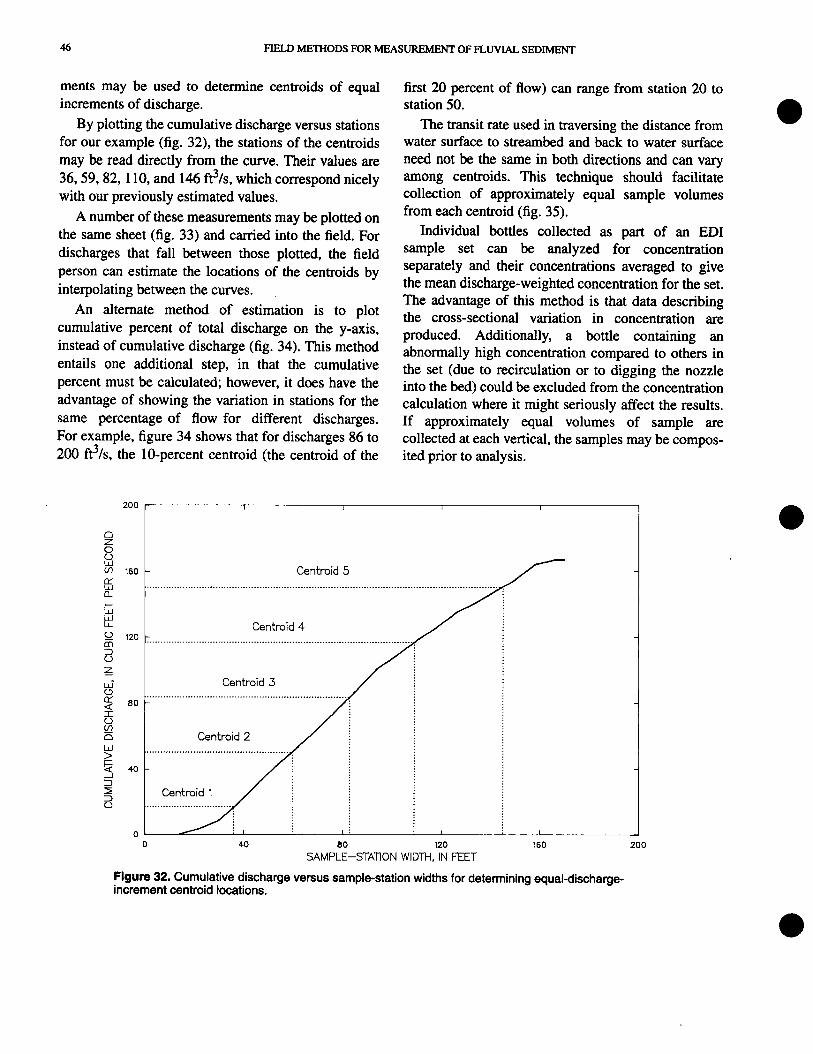
By plotting the cumulative discharge versus stations for our example (fig. 32), the stations of the centroids may be read directly from the curve. Their values are 36,59,82, 110, and 146 ft3/s, which correspond nicely with our previously estimated values.

A number of these measurements may be plotted on the same sheet (fig. 33) and carried into the field. For discharges that fall between those plotted, the field person can estimate the locations of the centroids by interpolating between the curves.

An alternate method of estimation is to plot

The transit rate used in traversing the distance from water surface to streambed and back to water surface need not be the same in both directions and can vary among centroids. This technique should facilitate collection of approximately equal sample volumes from each centroid (fig. 35).

cumulative percent of total discharge on the y-axis, instead of cumulative discharge (fig. 34). This method entails one additional step, in that the cumulative percent must be calculated; however, it does have the advantage of showing the variation in stations for the same percentage of flow for different discharges. For example, figure 34 shows that for discharges 86 to 200 ft3/s, the lo-percent centroid (the centroid of the

Individual bottles collected as part of an EDI sample set can be analyzed for concentration separately and their concentrations averaged to give the mean discharge-weighted concentration for the set. The advantage of this method is that data describing the cross-sectional variation in concentration are produced. Additionally, a bottle containing an abnormally high concentration compared to others in the set (due to recirculation or to digging the nozzle into the bed) could be excluded from the concentration calculation where it might seriously affect the results. If approximately equal volumes of sample are collected at each vertical, the samples may be composited prior to analysis.

Centroid 3

Centroid 2

0 40 80

SAMPLE-STATION WIDil-(1;2No FEET 160 200

Figure 32. Cumulative discharge versus sample-station widths for detemining equal-discharge- increment centroid locations.

SEDIMENT-SAMPLING TEXXNIQUES 47

&!!> - - - -

,

/-

0 40 80 120 160 200 SAMPLE-STATION WIDTH, IN FEET

Figure 33. Cumulative discharge versus sample-station widths for determining equal-discharge- increment centroid locations. Multiple discharge-measurement plots allow users to estimate centroid locations by interpolating between curves.

g - t

70 Centroid 4 // . . . . . . . . . . . . . . . . . . . . . . . . . . . . . . . . . . . . . . . . . . . . . . . . . . . . . . . . . . . . . . . . . . . . . . . r . . . . . f

SAMPLE-STATION WIDTH, IN FEET 200 240

Figure 34. Cumulative percent of discharge versus sample=station widths for determining equal- discharge-increment centroid locations.

FIELD METHODS FOR MEASUREMENT OF FLLMAL SEDIMENT

EXPLANATION

RT Transit rate at each centroid (not equal)

V Volume collected at each centrold (equal)

A f Centroid in each increment (samples collected)

Vn

R

Figure 35. Vertical transit rate relative to sample volume collected at each equal-discharge-increment centroid.

The streambed of a sand-bed stream characteristi- cally shifts radically, at single points and across segments of the width, over a period of weeks or in a matter of hours. This not only makes it impossible to establish cumulative discharge or cumulative percentage of discharge versus station curves applicable from one visit to the next, but also makes it impossible to be certain the discharge distribution does not change between the water-discharge measurement and the sediment sampling (see Guy, 1970, fig. 15).

The Equal-Width-Increment Method

A cross-sectional suspended-sediment sample obtained by the equal-width-increment (EWI) method requires a sample volume proportional to the amount of flow at each of several equally spaced verticals in the cross section. This equal spacing between the verticals (EWI) across the stream and sampling at an equal transit rate at all verticals yields a gross sample volume proportional to the total streamflow. It is important, obviously, to keep the same size nozzle in the sampler for a given measurement. This method was first used by B.C. Colby in 1946 (Federal Inter-

Agency Sedimentation Project, 1963b, p. 41) and is used most often in shallow, wadable streams and (or) sand-bed streams where the distribution of water discharge in the cross section is not stable. It also is useful in streams where tributary flow has not completely mixed with the main-stem flow.

The number of verticals required for an EWI sediment-discharge measurement depends on the distribution of concentration and flow in the cross section at the time of sampling, as well as on the desired accuracy of the result. On many streams, both statistical approaches and experience are needed to determine the desirable number of verticals. Until such experience is gained, the number of verticals used should be greater than necessary. In all cases, a minimum of 10 verticals should be used for streams over 5 feet wide. For streams less than 5 feet wide, as many verticals as possible should be used, as long as they are spaced a minimum of 3 inches apart, to allow for discrete sampling of each vertical and to avoid overlaps. Through general experience with similar streams, field personnel can estimate the required minimum number of verticals to yield a desired level

SEDIMJZNT-SAIblFUNGTEcHNIQ~ 49

of accuracy. For all but the very wide and shallow streams, a maximum of 20 verticals is usually ample.

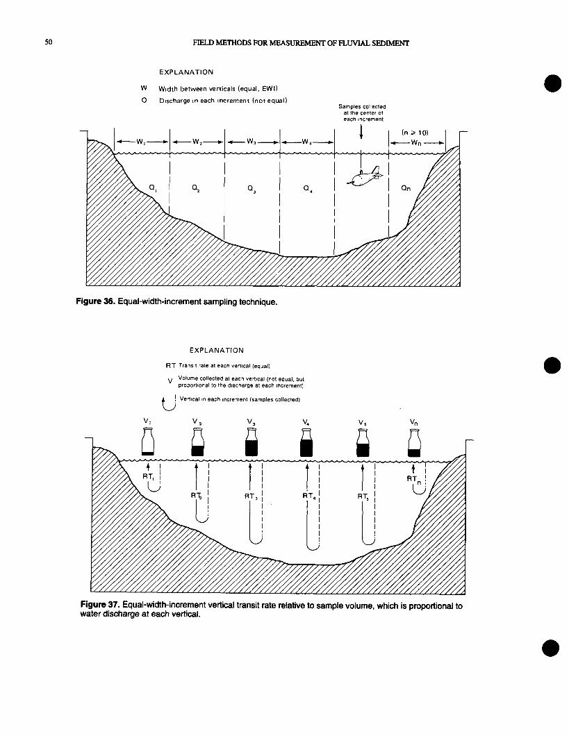
The width of the increments to be sampled, or the distance between verticals, is determined by dividing the stream width by the number of verticals necessary to collect a discharge-weighted suspended-sediment sample representative of the sediment concentration of the flow in the cross section (fig 36). For example, if the stream width determined from the tagline, cableway, or bridge-rail markings at the sample cross section is 160 feet, and the number of verticals necessary is 10, then the width (W) of each sampled increment would be 16 feet. The sample station within each width increment is located at the center of the increment (W/2), beginning at a location of 8 feet from the bank nearest the initial point for width measurement. The verticals then are spaced 16 feet apart, resulting in sample stationing at 8, 24, 40, 56, 72, 88, 104, 120, 136, and 152 feet of width. However, in the event the width increment results in a fractional measurement, the width can be rounded to the nearest integer that will yield a whole numbered station for the initial sample vertical. That is, if the increment computation yields a width of 15.5 feet, the nearest integer width would be 16 feet, and the initial vertical would be located at 8 feet from the bank; the stationing would be similar to the previous example. Results of samples obtained using this nonideal stationing will not be measurably affected because alterations in width occur in the increments nearest the streambank, where flow velocity is low compared to midstream increments.

The EWI sampling method requires that- all verticals be traversed using the transit rate (fig. 37) established at the deepest and fastest vertical in the cross section. The descending and ascending transit rates must be equal during the sampling traverse of each vertical, and they must be the same at all verticals. By using this equal-transit-rate technique with a standard depth- or point-integrating sampler at each vertical, a volume of water proportional to the flow in the vertical will be collected (fig. 37).

It is often difficult to maintain an equal transit rate when collecting samples while wading. The authors have found the following procedure to be effective in alleviating this difficulty. The field person should hold the sampler at a reference point on the body (for example, the hip), at which level the downward and upward integration is started and finished (even though part of the traverse is in air). The same reference point

should be used at each vertical, allowing the same amount of time to elapse during the round trip traverse of the sampler (regardless of the stream depth encoun- tered). In this manner, the transit rate will remain constant for the entire cross section. It should be remembered that the reference point at which the sampler traverse is started and stopped must be located above the water surface at the deepest vertical sampled and must be the same for each vertical.

Because the maximum transit rate must not exceed 0.4 vm (vm equals the mean ambient velocity in the sampled vertical) and because the minimum rate must be sufficiently fast to keep from overfilling any of the sample bottles, it is evident that the transit rate to be used for all verticals is limited by conditions at the vertical containing the largest discharge per foot of width (largest product of depth times velocity). A discharge measurement can be made to determine where this vertical is located, but generally, it is estimated by sounding for depth and acquiring a feel for the relative velocity with an empty sampler or wading rod. The transit rate required at the maximum discharge vertical then must be used at all other verticals in the cross section and is usually set to fill a bottle to the maximum sample volume in a round trip. It is possible to sample at two or more verticals using the same bottle if the bottle is not overfilled. If a bottle is overfilled, it must be discarded, and all verticals previously sampled using that bottle must be resampled, using a sufficient number of bottles to avoid overfilling. Note: a sample bottle is overfilled when the water surface in the bottle is above the nozzle or air exhaust with the sampler held level.

Advantages and Disadvantages of Equal-Discharge-Increment and Equal-Width-Increment Methods

Some advantages and disadvantages of both the ED1 and EWI methods have been mentioned in the previous discussion. It must be remembered, however, that both methods, if properly used, yield the same results. The advantages of the ED1 method are- 1. Fewer verticals are necessary, resulting in a

shortened collection time. 2. Sampling during rapidly changing stages is facili-

tated by the shorter sampling time. 3. Bottles comprising a sample set may be composited

for laboratory analysis when equal volumes of sample are collected from each vertical.

FIELD METHODS FOR MEASUREMENT OF FLUVIAL SEDIMENT

EXPLANATION

W Width between verticals (equal, EWI)

Q Dscharge in each Increment (not equal) Samples collected

at the center of each ,ncremen,

Figure 36. Equal-width-increment sampling technique.

EXPLANATION

RT Trawt rate at each verl~cal (equal)

v VOlume collected at each verbcal (not equal. but proporbonal lo the discharge at each mcrement)

!

tj

Verbcal m each mcrement (samples collected)

V, V2 VS vn

Figure 37. Equal-width-increment vertical transit rate relative to sample volume, which is proportional to water discharge at each vertical.

SEDIMENT-SAMF’JJNGTECHNIQUES 51

4. The cross-sectional variation in concentration can be determined if sample bottles are analyzed individually.

5. Duplicate cross-section samples can be collected simultaneously.

6. A variable transit rate can be used among verticals. The advantages of the EWI method are-

1. Previous knowledge of flow distribution in the cross section is not required.

2. Variations in the distribution of concentration in the cross section may be better defined, due to the greater number of verticals sampled.

3. Analytical time is reduced as sample bottles are cornposited for laboratory analysis.

4. This method is easily taught to and used by observers because the spacing of sample verticals is based on the easily obtained stream width, instead of on discharge.

5. Generally less total time is required on site, if no discharge measurement is deemed necessary and the cross section is stable.

From the previous discussion it is obvious that, while both methods have definite advantages, the advantages of one method are, in many cases, the disadvantages of the other. One major disadvantage of the EWI method that should be noted is the inability to adequately distinguish obviously bad samples in the sample set, as illustrated by the following:

Example:

Verticalibottle 1 2 3 4 5 6

Weight of sediment (g) 0.053 0.036 0.699 0.053 0.047 0.036

Weight of water se&- 350 300 325 330 360 355 ment mixture (g)

Concentration (mg/L) 151 120 2,150 161 131 101

Mean concentration

EWI and EDI methods (composited) = 457 mg/L

EDI method (individual bottles analyzed. concentration averaged) = 469 mg5

EDI method (individual bottles analyzed excluding bottle 3, concentration averaged) = 133 mgL

As this example shows, if the sample were an EWI sample and composited for analysis, the computed

mean concentration is 457 mg/L, which also is the mean concentration if the sample were considered as an ED1 sample similarly cornposited for analysis. If, in the case of the ED1 sample, the individual bottles were analyzed, normal computation would result in a mean concentration of 469 mg/L. From the data, bottle 3 appears to have been enriched and is not consistent with the other data points for this cross section. By exercising the flexibility of the ED1 method and eliminating the number 3 bottle, the mean concentration of the remaining five bottles is computed to be 133 mgL, which is probably more consistent with the actual mean concentration in the cross section.

Point Samples

A point sample is a sample of the water-sediment mixture collected from a single point in the cross section. It may be collected using a point-integrating sampler.

Point-integrated samples may be collected using one of the point-integrating samplers previously discussed. Data obtained in this manner may be used to define the distribution of sediment in a single vertical, such as the observer’s fixed station, the vertical and horizontal distribution of sediment in a cross section, and the mean spatial sediment concentration.

The purpose for which point samples are to be collected determines the collection method to be used. If samples are collected for the purpose of defining the horizontal and vertical distribution of concentration and (or) particle size, samples collected at numerous points in the cross section, with any of the “P” type samplers, will be sufficient. Normally, 5 to 10 verticals are sufficient for horizontal definition. Vertical distribution can be adequately defined by obtaining samples from a number of points in each sample vertical. Specifically, samples should be taken at the surface, from 1 foot above the bed point, with the sampler touching the bed, and from 6 to 10 additional points in the vertical above the l-foot-above-bed point. Each individual point sample should be analyzed separately. The results then can be plotted on a cross section relative to their instream location.

If point samples are collected to define the mean concentration in a vertical, 5 to 10 samples should be collected from the vertical. The sampling time for each sample (the time the nozzle is open) must be equal.


This will ensure that samples collected are proportional to the flow at the point of collection. These samples then are cornposited for laboratory analysis. If the ED1 method is used to define the stationing of the verticals, the sampling time may be varied among verticals. If the EWI method is used to determine the location of verticals, a constant sampling time for samples from all verticals must be used.

Number of Verticals

The number of suspended-sediment sampling verticals at a measuring site may depend on the kind of information needed in relation to the physical aspects of the river. For example, to determine the distribution of sediment concentration or particle size across the stream, it is necessary to sample at several verticals. The number of verticals necessary to define such a cross-sectional distribution depends on the accuracy being sought and on the systematic variation of sediment concentration at different verticals across the stream.

As noted previously, suspended-sediment samplers are designed to accumulate a sample that is directly proportional to the stream discharge or velocity. The accumulated sample may be from a point in the stream cross section, a vertical line between the surface and streambed, or several such vertical lines across the entire stream cross section. Such a sample then can be considered to be representative of some element of cross-sectional flow, whether it be a few square feet adjacent to the point sample, a few square feet adjacent to both sides of a vertical line, or the area of the entire flow summed by several vertical lines. The number of verticals sampled must be adequate to represent the cross section in the sample. The number of sample bottles to be collected will depend on the kind of analysis to be made in the laboratory, and the location of the sampling verticals will depend on the concentration and size distribution of sediment moving through the stream cross section.

Both ED1 and EWI methods of sediment-discharge measurement obtain a water-discharge weighted sample at each vertical. The volumetric sum from all verticals yields a sample volume proportional to the water discharge for the stream. Remember that all or nearly all of the concentration variations at different verticals across the stream may be the result of non- uniform distribution of sand-sized material and that finer sediments are generally more uniformly

dispersed throughout the section. If the section is close to a tributary, mixing of main stream and tributary flows may not be complete. Therefore, locating sampling sections downstream from tributary inflows should be avoided.

Colby (1964) showed that the discharge of sand is approximately proportional to the third power of the mean velocity, with constant temperature and a given particle-size distribution for a range of velocity from about 2 to 5 ft/s and within some reasonable range of depths. Thus, Q, = klv3, in which Q, is the discharge of sand per unit width; kl is a constant for a given depth, particle size, and temperature; and v is the mean velocity. The sand discharge can be written as Q, = kpzvd, in which k2 is another constant, c is the mean discharge-weighted concentration in the sampled vertical, and d is the total sampled depth. Solving for c gives

k 2

c=t%

Thus, the variability of concentration at different sampling verticals should be closely related to the variability of v*/d. In order to have a v?d index useful for comparison among all streams, the compound ratio

v2d(IMX) - is suggested, v2d

where [v2/dtmm ] is the ratio from the vertical having the maximum 3 /d, and v?d is the ratio of the mean velocity squared to the mean depth of the whole stream cross section. The mean velocity and mean depth are computed and available from water- discharge measurements.

Based on the G/d index concepts of variability, P.R. Jordan used data from Hubbell and others (1956) to prepare a nomograph (fig. 38) that indicates the number of sampling verticals required for a desired maximum acceptable relative standard error (sampling error) based on the percentage of sand and the v*/d index. In the example illustrated by figure 38, the acceptable relative standard error is 15 percent, the sample is 100~percent sand, the v?d index is 2.0, and the required number of verticals is seven. Notice that if the sediment were Xl-percent sand, the same results

SEDIMENT-SAMPLINGTECHNIQIJES 53

PERCENTAGE OF SAN0 )

‘I

I __

50 25 0 I

\

\

I

\

\ \ I

I I

I

~

-

30

RELATIVE STANDARD ERROR, IN PERCENT (maximum acceptable)

-

V’/D Index= Vf/D (max)

82/D

10 20 30 40

NUMBER OF VERTICALS

Figure 38. Nomograph to determine number of sampling verticals required to obtain results within an acceptable relative standard error.

could be obtained with three verticals; or, if seven verticals were used with 50-percent sand, the relative standard error would be about 8 percent. When the discharge of sand-sized particles is of primary interest, the 100~percent line should be used regardless of the amount of fines in the sample.

Transit Rates for Suspended-Sediment Sampling

The sample obtained by passing the sampler throughout the full depth of a stream is quantitatively weighted according to the velocity through which it passes. Therefore, if the sampling vertical represents a specific width of flow, the sample is considered to be discharge weighted because, with a uniform transit rate, suspended sediment carried by the discharge throughout the sampled vertical is given equal time to enter the sampler. In previous writings, the point was made to keep the transit rate of the samplers constant throughout at least a single direction of travel.

The maximum transit rate used with any depth- integrating sampler must be regulated to ensure the collection of representative samples. If the transit rate is too fast, the rate of air-volume reduction in the sample container is less than the rate of increase in hydrostatic pressure surrounding the sampler, and water may be forced into the intake or air exhaust.

Additionally, an excessive transit rate can result in intake velocities less than the stream velocity at the intake, due to a large entrance angle between the nozzle and streamflow lines caused by the vertical movement of the sampler in the flow (Federal Inter- Agency Sedimentation Project, 1952). To alleviate these problems, transit rates should never exceed 0.4 of the mean velocity (0.4 vm) in a vertical. Figures 39, 40, and 41 can be used to determine the appropriate transit rate to be used with a given nozzle-size/sample- container-size combination. These figures show that maximum transit rates vary from about 0.1 v, to the approach angle limit of 0.4 v,, previously noted. This variation is a function of both nozzle size and sample- container size. The smaller nozzle (l/8 inch) is greatly affected by approach angle intake velocity reductions; figures 39 and 40 show that the transit rate decreases directly with nozzle size. Also, by comparison of figures 39 and 40, it is obvious that transit rates are inversely affected by sample-container size because an increase in sampler container size produces a decrease in allowable transit rate due to the effects of hydrostatic pressure compressing the air within the container during the downward transit. Figures 39.40, and 41 were constructed using procedures from F.I.S.P. (1952), Report 6, Section 8, as contained in the

54

20

25

30 I 1 I I -_ --

0.0 0.1 0.7. 0.5 0.4 OS

TRANSIT RATE DIVIDED BY MEAN VELOClTY

FlELJ3METHODSpORMEAS- OF FLUVIAL SEDIMENT

Permissible Range

0

5

10

is

z l5

ii

20

25

30

B

0.0 0.1

TRANSIT R% DIVIDED BY M& VELOCITY 0.4 0.5

A

Figure 39. Variation of range of transit rate to mean velocity ratio versus depth relative to nozzle site for pint-size sample container. A, l/Wwh nozzle. 8,3H6-inch nozzle. c, l/l-inch nozzle.

s~~m+fm-r-s~MP~G TFXHNIQUES 55

0

5

10

6

It

z '5 -

E

x

20

2.5

30

-..

Compression depth limit ;F

/’ Depth-integration samplers)

;g iq

______,__.,____..,_........,.,......,.,.,................................,.......,..............................................~... - . . . . . j

0.0 0.1

TRANSIT RKE DIVIDED BY M&L VELOCITY 0.4 lJ.5

Figure 39. Variation of range of transit rate to mean velocity ratio versus depth relative to nozzle size for pint-size sample container. A, l/&inch nozzle. 6, 3/16-inch nozzle. C, l/4-inch nozzle-Continued.

sampling instructions for the D-74 depth-integrating sampler.

Figure 42 is a graphic presentation of the procedure to be followed when constructing transit-rate graphs similar to those presented in figures 39, 40, and 41, using the following nomenclature and equations: An = Area of intake nozzle at entrance; square feet

l/8 inch = 8.52 x 10S5, 3/16 inch = 19.2 x lo-‘, l/4 inch = 34.1 x 10W5, and 5/16 inch = 53.3 x 1o-5

4 = Stream depth where bottom compression limit equals surface compression; feet

hl = Atmospheric pressure at water surface = 34 feet at sea level

Q max = Maximum sample volume; cubic feet (pint bottle, 420 mL = 0.015 ft3; quart bottle, 800 mL = 0.028 ft3; 3-liter bottle, 2,700 mL = 0.095 ft3)

Q min = Minimum sample volume; cubic feet (pint bottle, 300 mL = 0.011 ft3; quart bottle, 650 mL = 0.023 ft3; 3-liter bottle, 2,000 mL = 0.071 ft3>

‘b = Relative velocity near stream bottom; feet per second

RT = Transit rate of sampler; feet per second (rising rate equals lowering rate for EWI method)

‘s = Relative velocity at stream surface; feet per second

Vl = Volume of container; cubic feet 1 pint = 0.01671 ft3, 1 quart = 0.03342 ft3, and 3-liter bottle = 0.105 ft3

V,,, = Mean stream velocity in vertical; feet per second

RT Anrbhl Point 1 v = - m Vl

RT A”Ul Point 2 r = - m Vl

Point 3 d, = h&T,) =

‘b+l

15 feet, for assumed velocity profile in figure 42.

0

5

10

8

i l5

Fi

20

25

30

A

Compression depth limit Depth-integration samplers)

I I I 0.0 0.1 0.2 0.3 0.4 0.5

TRANSIT RATE DIVIDED BY MEAN VELOCITY

10

z 15 35 E x

20

25

30

Xompression depth limit 1 (Depth-lntegmtlon samplers)

B

0.0 0.1 0.2

TRANSIT RATE DIVIDED BY Mi% VELOCITY 0.4 0.5

Figure 40. Variation of range of transit rate to mean velocity ratio versus depth relative to nozzle size for quart-size sample container. A, 1/84nch nozzle. 6,3/1&inch nozzle. C, M-inch nozzle.


0.0 0.1 0.2 0.3 0.4 0.5


Figure 40. Variation of range of Wan&ate to mean velocity ratio versus depth relative to nozzle size for quart-size sample container. A, l/8-inch nozzle B, 3/l 8-inch nozzle. C, l/4-inch nozzle- Continued.

RT 20 A,, Point 4 r = -

m Q max

RT 20 A,, Point 5 v = -

m QIllill

For points 4 and 5, the depth is arbitrarily taken at 10 feet to facilitate plotting. Also, the following sample vertical velocity profile is assumed:

Relative depth

surface .l .2 .3 .4 .5 .6 .7 .8 .9

1 .O bottom

Velocity/ mean velocity

in vertical

1.16 1.17 1.16 1.15 1.10 1.05 1.0 .94 34 .67 .5

The technique for use of figures 39, 40, and 41 to determine the transit rate to be used in a given situation depends upon (1) the depth of the sample vertical, (2) the mean velocity of the vertical, (3) the nozzle size being used, and (4) the sample-bottle size used in the sampler. An example of transit-rate determination is presented in figure 43. The nozzle size and sample-bottle size must be known so the proper figure can be selected. In this case, a 3 /16-inch nozzle and l-pint bottle will be used. The depth and mean velocity of the sample vertical also must be known. For this example, a depth of 10 feet and mean velocity of 2 ft/s are assumed. To determine transit rate for this example (1) select the depth of the sample vertical (10 feet); (2) draw a line perpendicular to the depth on the vertical scale that terminates at the center of the optimum range; (3) read the value of RT/V, from the horizontal scale corresponding to this point (0.28); and (4) multiply the RT/V, value by the mean velocity (V, = 2 ft/s) to determine the transit rate (RT = 0.56 ft/s). Note that, if the same nozzle, depth, and mean velocity were used with a quart sample container in lieu of the pint container (fig. 4OB), an RT value of 0.30 ft/s would be used, reducing the transit rate by almost one-half.

58 FIELD METHODS FOR MEASURJNENT OF FLUVL4L SEDIMENT

5

10

L

I?

z _ '5

F

4 n

20

25

30 0.0 0.1 0.2 0.3 0.4 0.5


Figure 41. Range of transit rate to mean velocity ratio versus depth for 5/l 6-inch nozzle on a 3-liter sample bottle.

0

5

Optimum range-y///

Compression depth limit (Depth-integration samplers)

L ........................................................... .................................. .................................................................................................

Absolute maxim.um depth (D e pth-’ In e t gratlon sample:; ..

Numbered boxes refer to equation calculation points; see discussion in text.

Air exhaust ; overflow j limit ?l

25 I\ / Approach angle j I imit

30 0.0 0.1 0.2 0.3 0.4 0.5 0.6


Figure 42. Construction of a transit-rate detemination graph (see text for explanation of numbered points).

SEDIMFNT-SAMPLING TEXXNIQUES 59

t=i z - ‘5 6 4 0

20

25

30 _ _ I I

0.0 0.1 0.2

Depth of vertical

m 1 0.3 0.4 0.5


Figure 43. Example of transit rate determination using graph developed for 3/l 6-inch nozzle and a l-pint sample container (see text for discussion).

Use of transit rates determined from the optimum range of figures 39, 40, or 41 will yield a representative sample of adequate volume to provide for laboratory analysis and avoid overfilling. In some instances, however, sampler operation within the optimum range is not possible. Under these conditions, operation using a transit rate determine.. from the permissible range is acceptable. In thes cases, it should be realized that a represent&iv:. sample can still be obtained, but the sample volume may be less than adequate for laboratory purposes and, therefore, more integrations may be required at each vertical to obtain the necessary volume of sample.

Additional explanation and qualifications with respect to the transit rate for depth-integrated suspended-sediment sampling include the following:

1. For cable-suspended samplers, the instantaneous actual transit rate, RT,, may differ considerably from the computed rate, RT, if V, exceeds about 6 ft/s and if the sampler is suspended from more than 20 feet above the water surface. Under such conditions, the sampler is dragged downstream, and the indicated depth is greater than the true depth. Corrections for indicated depth are given by Buchanan and Somers (1969, p. 50-56) for various angles and lengths of

sounding line used for suspension of a weight in deep, swift water. The correct depth then would be used to enter in figures 39, 40, and 41 to determine the appropriate transit rate.

2. In theory, the allowable RT may be greater than 0.4 V,, and sampling depth thereby increased if the sampler is cable suspended and capable of being tilted somewhat in the direction of vertical movement (that is, nozzle is slightly down when sampler is lowered and slightly up when sampler is raised, due to the effect of vertical forces on the horizontal tail-fin stabilizer). On the other hand, if the sampler cannot be tilted, the velocity at the bottom of the vertical is much less than V,, and there is a heavy concentration of suspended sand near the bed, the use of an RT value near the 0.4 V, limitation may cause RT to approach or even exceed the actual velocity near the bed and thus cause an excessive error in the collection of sand particles. The approach-angle theoretical depth limits will, of course, be less if either the downward or the upward transit rates, RTd or RT,, are different from RT. However, determining the attitude of the sampler during actual use is difficult at best and impossible under turbid flow conditions. For this reason, varying either RT or sampling beyond recommended limits is

60 FIELD METHODS FOR MEASUREMENT OF FLUVIAL, SEDIMENT

not advisable and probably not necessary because small errors during descent will probably be cancelled during ascent.

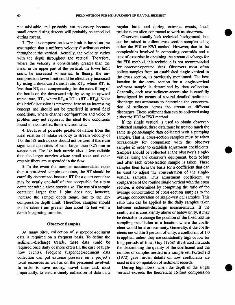
3. The air-compression lower limit is based on the assumption that a uniform velocity distribution exists throughout the vertical. Actually, the velocity varies with the depth throughout the vertical. Therefore, where the velocity is considerably greater than the mean in the upper part of the vertical, the lower limit could be increased somewhat. In theory, the air- compression lower limit could be effectively increased by using a downward transit rate, RT,, where RTd is less than RT, and compensating for the extra filling of the bottle on the downward trip by using an upward transit rate, RT,, where RT,, = RT + (RT - RTd). Note: this brief discussion is presented here as an interesting concept and should not be practiced in actual field conditions, where channel configuration and velocity profiles may not represent the ideal flow conditions found in a controlled flume environment.

4. Because of possible greater deviation from the ideal relation of intake velocity to stream velocity of 1 .O, the l/8-inch nozzle should not be used if there are significant quantities of sand larger than 0.25 mm in suspension. The l/8-inch nozzle also is less reliable than the larger nozzles where small roots and other organic fibers are suspended in the flow.

5. In the event the sampler accommodates other than a pint-sized sample container, the RT should be carefully determined because RT for a quart container may be nearly one-half of that acceptable for a pint container with a given nozzle size. The use of a sample container larger than 1 pint does not, however, increase the sample depth range, due to the air- compression depth limit. Therefore, samples should not be taken from greater than about 15 feet with a depth-integrating sampler.

Observer Samples

At many sites, collection of suspended-sediment data is required on a frequent basis. To define the sediment-discharge trends, these data could be required once daily or more often (in the case of high- flow events). Frequent suspended-sediment data collection can put extreme pressure on a project’s fiscal resources as well as on the personnel involved. In order to save money, travel time and, most importantly, to ensure timely collection of data on a

regular basis and during extreme events, local residents are often contracted to work as observers.

Observers usually lack technical background, but can be trained to collect cross-section samples using either the EDI or EWI method. Hosvever, due to the complexities involved in computing centroids and a lack of expertise in obtaining the stream discharge for the ED1 method, this technique is not recommended for observer-operated sites. Observers most often collect samples from an established single vertical in the cross section, as previously mentioned. The best location in the cross section for a single-vertical sediment sample is determined by data collection. Generally, each new sediment-record site is carefully investigated by means of several detailed sediment- discharge measurements to determine the concentration of sediment across the stream at different discharges. These sediment data can be collected using either the ED1 or EWI method.

If the single vertical is used to obtain observer- collected samples, these data must be treated much the same as point-sample data collected with a pumping sampler. That is, cross-section samples must be taken occasionally for comparison with the observer samples in order to establish adjustment coefficients. Samples should be collected at the observer’s single- vertical using the observer’s equipment, both before and after each cross-section sample is taken. These samples then form the basis for a coefficient that can be used to adjust the concentration of the single- vertical samples. This adjustment coefficient, or comparison of the routine single vertical with the cross section, is determined by computing the ratio of the average concentration of cross-section samples to the average concentration of single-vertical samples. This ratio then can be applied to the daily samples taken between sediment-discharge measurements. If the coefficient is consistently above or below unity, it may be desirable to change the position of the fixed routine sampling installation to a location where the coefficient would be at or near unity. Generally, if the coefficients are within 5 percent of unity, a coefficient of 1.0 is applied, unless they are consistently high or low for long periods of time. Guy (1968) illustrated methods for determining the quality of the coefficient and the number of samples needed in a sample set. Porterfield (1972) gave further details on how coefficients are used in the computation of sediment records.

During high flows, when the depth of the single vertical exceeds the theoretical 15-foot compression


depth limit of the depth-integrating sampler, the observer should try to obtain a sample by altering the technique to collect the most representative sample possible. The best collection technique under these conditions would be to depth integrate 0.2 of the vertical depth (0.2& or a lo-foot portion of the vertical. These samples then can be checked and verified by collecting a set of reference samples with a point-integrating sampler. By reducing the sampled depth during periods of high flow, the transit rate can be maintained at 0.4 V, or less in the vertical, and a partial sample can be collected without overfilling the sample container, even under conditions of higher velocities that usually accompany increases in discharge.

Sampling Frequency, Sediment Quantity, Sample Integrity, and Identification

Sampling Frequency

When should suspended-sediment samples be taken? How close can samples be spaced in time and still be meaningful? How many extra samples are required during a flood period? These are some questions that must be answered because timing of sample observations is as important to record computations (see Porterfield, 1972) as is the technique for taking them. Answering such questions is relatively easy for those who compute and assemble the records because they have the historical record before them and can easily see what is needed. However, the field person frequently does not have this record and certainly cannot know what the conditions will be in the future.

Observers should be shown typical hydrographs or recorder charts of their stations or of nearby stations to help them understand the importance of timing their samples so that each sample yields maximum information. The desirable time distribution for samples depends on many factors, such as the season of the year, the runoff characteristics of the basin, the adequacy of coverage of previous events, and the accuracy of information desired or dictated by the purpose for which the data are collected.

For many streams, the largest concentrations and 70 to 90 percent of the annual sediment load occur during spring runoff; on other streams, the most important part of the sediment record may occur during the period of the summer thunderstorms or during winter storms. The frequency of suspended-sediment

sampling should be much greater during these periods than during the low-flow periods. During some parts of these critical periods, hourly or more frequent sampling may be required to accurately define the trend of sediment concentration. During the remainder of the year, the sampling frequency can be stretched out to daily or even weekly sampling for adequate definition of concentration. Hurricane or thunderstorm events during the summer or fall require frequent samples during short periods of time. Streams having long periods of low or intermittent flow should be sampled frequently during each storm event because most of the annual sediment transport occurs during these few events.

During long periods of rather constant or gradually varying flow, most streams have concentrations and quantities of sediment that vary slowly and may, therefore, be adequately sampled every 2 or 3 days; in some streams, one sampling a week may be adequate. Several samplings a day may occasionally be needed to define the diurnal fluctuation in sediment concentration. Fluctuations in power generation and evapotrans- piration can cause diurnal fluctuations. Sometimes diurnal temperature fluctuations result in a snow and ice freeze/thaw cycle causing an accompanying fall and rise in stage. Diurnal fluctuations also have been noted in sand-bed streams when water-temperature changes cause a change in flow regime and a drastic change in bed roughness (Simons and Richardson, 1965).

The temporal shape of the hydrograph is an indicator of how a stream should be sampled. Sampling twice a day may be sufficient on the rising stage if it takes a day or more for a stream to reach a peak rate of discharge. During the peak, samples every few hours may be needed. During the recession, sampling can be reduced gradually until normal sampling intervals are sufficient.

The sediment-concentration peak may occur at any time relative to the water discharge; it may coincide with the water-discharge peak or occur several days prior to or after it. Hydrographs for large rivers, especially in the Midwest, typically show water- discharge peaks occurring several days after a storm event. If the sediment concentration has its source locally, the sediment peak can occur a day or more prior to the water-discharge peak. In this case, the receding limb of the sediment-concentration curve will nearly coincide with the lagging water-discharge peak. In this event, intensive sampling logically should

twri 3-c2 - part 3 - usgs

Documents