tyn myint-u lokenath debnath linear partial …tyn myint-u lokenath debnath linear partial...
TRANSCRIPT


Tyn Myint-ULokenath Debnath
Linear Partial
Differential Equations
for Scientists and Engineers
Fourth Edition
BirkhauserBoston • Basel • Berlin

Tyn Myint-U5 Sue TerraceWestport, CT 06880USA
Lokenath DebnathDepartment of MathematicsUniversity of Texas-Pan American1201 W. University DriveEdinburgh, TX 78539USA
Cover design by Alex Gerasev.
Mathematics Subject Classification (2000): 00A06, 00A69, 34B05, 34B24, 34B27, 34G20, 35-01,35-02, 35A15, 35A22, 35A25, 35C05, 35C15, 35Dxx, 35E05, 35E15, 35Fxx, 35F05, 35F10, 35F15,35F20, 35F25, 35G10, 35G20, 35G25, 35J05, 35J10, 35J20, 35K05, 35K10, 35K15, 35K55, 35K60,35L05, 35L10, 35L15, 35L20, 35L25, 35L30, 35L60, 35L65, 35L67, 35L70, 35Q30, 35Q35, 35Q40,35Q51, 35Q53, 35Q55, 35Q58, 35Q60, 35Q80, 42A38, 44A10, 44A35 49J40, 58E30, 58E50, 65L15,65M25, 65M30, 65R10, 70H05, 70H20, 70H25, 70H30, 76Bxx, 76B15, 76B25, 76D05, 76D33,76E30, 76M30, 76R50, 78M30, 81Q05
Library of Congress Control Number: 2006935807
ISBN-10: 0-8176-4393-1 e-ISBN-10: 0-8176-4560-8ISBN-13: 978-0-8176-4393-5 e-ISBN-13: 978-0-8176-4560-1
Printed on acid-free paper.
c©2007 Birkhauser BostonAll rights reserved. This work may not be translated or copied in whole or in part without the writtenpermission of the publisher (Birkhauser Boston, c/o Springer Science+Business Media LLC, 233Spring Street, New York, NY 10013, USA) and the author, except for brief excerpts in connection withreviews or scholarly analysis. Use in connection with any form of information storage and retrieval,electronic adaptation, computer software, or by similar or dissimilar methodology now known orhereafter developed is forbidden.The use in this publication of trade names, trademarks, service marks and similar terms, even if theyare not identified as such, is not to be taken as an expression of opinion as to whether or not they aresubject to proprietary rights.
9 8 7 6 5 4 3 2 1
www.birkhauser.com (SB)
To the Memory of
U and Mrs. Hla Din
U and Mrs. Thant
Tyn Myint-U
In Loving Memory of
My Mother and Father
Lokenath Debnath

“True Laws of Nature cannot be linear.”“The search for truth is more precious than its possession.”“Everything should be made as simple as possible, but not a bit sim-
pler.”
Albert Einstein
“No human investigation can be called real science if it cannot be demon-strated mathematically.”
Leonardo Da Vinci
“First causes are not known to us, but they are subjected to simpleand constant laws that can be studied by observation and whose study isthe goal of Natural Philosophy ... Heat penetrates, as does gravity, all thesubstances of the universe; its rays occupy all regions of space. The aim ofour work is to expose the mathematical laws that this element follows ... Thedifferential equations for the propagation of heat express the most generalconditions and reduce physical questions to problems in pure Analysis thatis properly the object of the theory.”
James Clerk Maxwell
“One of the properties inherent in mathematics is that any real progressis accompanied by the discovery and development of new methods and sim-plifications of previous procedures ... The unified character of mathematicslies in its very nature; indeed, mathematics is the foundation of all exactnatural sciences.”
David Hilbert
“ ... partial differential equations are the basis of all physical theorems.In the theory of sound in gases, liquid and solids, in the investigationsof elasticity, in optics, everywhere partial differential equations formulatebasic laws of nature which can be checked against experiments.”
Bernhard Riemann
“The effective numerical treatment of partial differential equations isnot a handicraft, but an art.”
Folklore
“The advantage of the principle of least action is that in one and thesame equation it relates the quantities that are immediately relevant notonly to mechanics but also to electrodynamics and thermodynamics; thesequantities are space, time and potential.”
Max Planck

“The thorough study of nature is the most ground for mathematicaldiscoveries.”
“The equations for the flow of heat as well as those for the oscillations ofacoustic bodies and of fluids belong to an area of analysis which has recentlybeen opened, and which is worth examining in the greatest detail.”
Joseph Fourier
“Of all the mathematical disciplines, the theory of differential equationis the most important. All branches of physics pose problems which can bereduced to the integration of differential equations. More generally, the wayof explaining all natural phenomena which depend on time is given by thetheory of differential equations.”
Sophus Lie
“Differential equations form the basis for the scientific view of theworld.”
V.I. Arnold
“What we know is not much. What we do not know is immense.”“The algebraic analysis soon makes us forget the main object [of our
research] by focusing our attention on abstract combinations and it is onlyat the end that we return to the original objective. But in abandoning one-self to the operations of analysis, one is led to the generality of this methodand the inestimable advantage of transforming the reasoning by mechanicalprocedures to results often inaccessible by geometry ... No other languagehas the capacity for the elegance that arises from a long sequence of ex-pressions linked one to the other and all stemming from one fundamentalidea.”
“It is India that gave us the ingenious method of expressing all numbersby ten symbols, each symbol receiving a value of position, as well as anabsolute value. We shall appreciate the grandeur of the achievement whenwe remember that it escaped the genius of Archimedes and Appolonius.”
P.S. Laplace
“The mathematician’s best work is art, a high perfect art, as daringas the most secret dreams of imagination, clear and limpid. Mathematicalgenius and artistic genius touch one another.”
Gosta Mittag-Leffler

Contents
Preface to the Fourth Edition . . . . . . . . . . . . . . . . . xvPreface to the Third Edition . . . . . . . . . . . . . . . . . xix
1 Introduction 11.1 Brief Historical Comments . . . . . . . . . . . . . . . . . 11.2 Basic Concepts and Definitions . . . . . . . . . . . . . . . 121.3 Mathematical Problems . . . . . . . . . . . . . . . . . . . 151.4 Linear Operators . . . . . . . . . . . . . . . . . . . . . . . 161.5 Superposition Principle . . . . . . . . . . . . . . . . . . . 201.6 Exercises . . . . . . . . . . . . . . . . . . . . . . . . . . . 22
2 First-Order, Quasi-Linear Equations and Method ofCharacteristics 272.1 Introduction . . . . . . . . . . . . . . . . . . . . . . . . . 272.2 Classification of First-Order Equations . . . . . . . . . . . 272.3 Construction of a First-Order Equation . . . . . . . . . . 292.4 Geometrical Interpretation of a First-Order Equation . . 332.5 Method of Characteristics and General Solutions . . . . . 352.6 Canonical Forms of First-Order Linear Equations . . . . 492.7 Method of Separation of Variables . . . . . . . . . . . . . 512.8 Exercises . . . . . . . . . . . . . . . . . . . . . . . . . . . 55
3 Mathematical Models 633.1 Classical Equations . . . . . . . . . . . . . . . . . . . . . 633.2 The Vibrating String . . . . . . . . . . . . . . . . . . . . 653.3 The Vibrating Membrane . . . . . . . . . . . . . . . . . . 673.4 Waves in an Elastic Medium . . . . . . . . . . . . . . . . 693.5 Conduction of Heat in Solids . . . . . . . . . . . . . . . . 753.6 The Gravitational Potential . . . . . . . . . . . . . . . . . 763.7 Conservation Laws and The Burgers Equation . . . . . . 793.8 The Schrodinger and the Korteweg–de Vries Equations . 813.9 Exercises . . . . . . . . . . . . . . . . . . . . . . . . . . . 83
4 Classification of Second-Order Linear Equations 914.1 Second-Order Equations in Two Independent Variables . 91
x Contents
4.2 Canonical Forms . . . . . . . . . . . . . . . . . . . . . . . 934.3 Equations with Constant Coefficients . . . . . . . . . . . 994.4 General Solutions . . . . . . . . . . . . . . . . . . . . . . 1074.5 Summary and Further Simplification . . . . . . . . . . . . 1114.6 Exercises . . . . . . . . . . . . . . . . . . . . . . . . . . . 113
5 The Cauchy Problem and Wave Equations 1175.1 The Cauchy Problem . . . . . . . . . . . . . . . . . . . . 1175.2 The Cauchy–Kowalewskaya Theorem . . . . . . . . . . . 1205.3 Homogeneous Wave Equations . . . . . . . . . . . . . . . 1215.4 Initial Boundary-Value Problems . . . . . . . . . . . . . . 1305.5 Equations with Nonhomogeneous Boundary Conditions . 1345.6 Vibration of Finite String with Fixed Ends . . . . . . . . 1365.7 Nonhomogeneous Wave Equations . . . . . . . . . . . . . 1395.8 The Riemann Method . . . . . . . . . . . . . . . . . . . . 1425.9 Solution of the Goursat Problem . . . . . . . . . . . . . . 1495.10 Spherical Wave Equation . . . . . . . . . . . . . . . . . . 1535.11 Cylindrical Wave Equation . . . . . . . . . . . . . . . . . 1555.12 Exercises . . . . . . . . . . . . . . . . . . . . . . . . . . . 158
6 Fourier Series and Integrals with Applications 1676.1 Introduction . . . . . . . . . . . . . . . . . . . . . . . . . 1676.2 Piecewise Continuous Functions and Periodic Functions . 1686.3 Systems of Orthogonal Functions . . . . . . . . . . . . . . 1706.4 Fourier Series . . . . . . . . . . . . . . . . . . . . . . . . . 1716.5 Convergence of Fourier Series . . . . . . . . . . . . . . . . 1736.6 Examples and Applications of Fourier Series . . . . . . . 1776.7 Examples and Applications of Cosine and Sine Fourier
Series . . . . . . . . . . . . . . . . . . . . . . . . . . . . . 1836.8 Complex Fourier Series . . . . . . . . . . . . . . . . . . . 1946.9 Fourier Series on an Arbitrary Interval . . . . . . . . . . 1966.10 The Riemann–Lebesgue Lemma and Pointwise
Convergence Theorem . . . . . . . . . . . . . . . . . . . . 2016.11 Uniform Convergence, Differentiation, and Integration . . 2086.12 Double Fourier Series . . . . . . . . . . . . . . . . . . . . 2126.13 Fourier Integrals . . . . . . . . . . . . . . . . . . . . . . . 2146.14 Exercises . . . . . . . . . . . . . . . . . . . . . . . . . . . 220
7 Method of Separation of Variables 2317.1 Introduction . . . . . . . . . . . . . . . . . . . . . . . . . 2317.2 Separation of Variables . . . . . . . . . . . . . . . . . . . 2327.3 The Vibrating String Problem . . . . . . . . . . . . . . . 2357.4 Existence and Uniqueness of Solution of the Vibrating
String Problem . . . . . . . . . . . . . . . . . . . . . . . . 2437.5 The Heat Conduction Problem . . . . . . . . . . . . . . . 248

Contents xi
7.6 Existence and Uniqueness of Solution of the HeatConduction Problem . . . . . . . . . . . . . . . . . . . . . 251
7.7 The Laplace and Beam Equations . . . . . . . . . . . . . 2547.8 Nonhomogeneous Problems . . . . . . . . . . . . . . . . . 2587.9 Exercises . . . . . . . . . . . . . . . . . . . . . . . . . . . 265
8 Eigenvalue Problems and Special Functions 2738.1 Sturm–Liouville Systems . . . . . . . . . . . . . . . . . . 2738.2 Eigenvalues and Eigenfunctions . . . . . . . . . . . . . . . 2778.3 Eigenfunction Expansions . . . . . . . . . . . . . . . . . . 2838.4 Convergence in the Mean . . . . . . . . . . . . . . . . . . 2848.5 Completeness and Parseval’s Equality . . . . . . . . . . . 2868.6 Bessel’s Equation and Bessel’s Function . . . . . . . . . . 2898.7 Adjoint Forms and Lagrange Identity . . . . . . . . . . . 2958.8 Singular Sturm–Liouville Systems . . . . . . . . . . . . . 2978.9 Legendre’s Equation and Legendre’s Function . . . . . . . 3028.10 Boundary-Value Problems Involving Ordinary Differential
Equations . . . . . . . . . . . . . . . . . . . . . . . . . . . 3088.11 Green’s Functions for Ordinary Differential Equations . . 3108.12 Construction of Green’s Functions . . . . . . . . . . . . . 3158.13 The Schrodinger Equation and Linear Harmonic
Oscillator . . . . . . . . . . . . . . . . . . . . . . . . . . . 3178.14 Exercises . . . . . . . . . . . . . . . . . . . . . . . . . . . 321
9 Boundary-Value Problems and Applications 3299.1 Boundary-Value Problems . . . . . . . . . . . . . . . . . . 3299.2 Maximum and Minimum Principles . . . . . . . . . . . . 3329.3 Uniqueness and Continuity Theorems . . . . . . . . . . . 3339.4 Dirichlet Problem for a Circle . . . . . . . . . . . . . . . . 3349.5 Dirichlet Problem for a Circular Annulus . . . . . . . . . 3409.6 Neumann Problem for a Circle . . . . . . . . . . . . . . . 3419.7 Dirichlet Problem for a Rectangle . . . . . . . . . . . . . 3439.8 Dirichlet Problem Involving the Poisson Equation . . . . 3469.9 The Neumann Problem for a Rectangle . . . . . . . . . . 3489.10 Exercises . . . . . . . . . . . . . . . . . . . . . . . . . . . 351
10 Higher-Dimensional Boundary-Value Problems 36110.1 Introduction . . . . . . . . . . . . . . . . . . . . . . . . . 36110.2 Dirichlet Problem for a Cube . . . . . . . . . . . . . . . . 36110.3 Dirichlet Problem for a Cylinder . . . . . . . . . . . . . . 36310.4 Dirichlet Problem for a Sphere . . . . . . . . . . . . . . . 36710.5 Three-Dimensional Wave and Heat Equations . . . . . . . 37210.6 Vibrating Membrane . . . . . . . . . . . . . . . . . . . . . 37210.7 Heat Flow in a Rectangular Plate . . . . . . . . . . . . . 37510.8 Waves in Three Dimensions . . . . . . . . . . . . . . . . . 379

xii Contents
10.9 Heat Conduction in a Rectangular Volume . . . . . . . . 38110.10 The Schrodinger Equation and the Hydrogen Atom . . . 38210.11 Method of Eigenfunctions and Vibration of Membrane . . 39210.12 Time-Dependent Boundary-Value Problems . . . . . . . . 39510.13 Exercises . . . . . . . . . . . . . . . . . . . . . . . . . . . 398
11 Green’s Functions and Boundary-Value Problems 40711.1 Introduction . . . . . . . . . . . . . . . . . . . . . . . . . 40711.2 The Dirac Delta Function . . . . . . . . . . . . . . . . . . 40911.3 Properties of Green’s Functions . . . . . . . . . . . . . . . 41211.4 Method of Green’s Functions . . . . . . . . . . . . . . . . 41411.5 Dirichlet’s Problem for the Laplace Operator . . . . . . . 41611.6 Dirichlet’s Problem for the Helmholtz Operator . . . . . . 41811.7 Method of Images . . . . . . . . . . . . . . . . . . . . . . 42011.8 Method of Eigenfunctions . . . . . . . . . . . . . . . . . . 42311.9 Higher-Dimensional Problems . . . . . . . . . . . . . . . . 42511.10 Neumann Problem . . . . . . . . . . . . . . . . . . . . . . 43011.11 Exercises . . . . . . . . . . . . . . . . . . . . . . . . . . . 433
12 Integral Transform Methods with Applications 43912.1 Introduction . . . . . . . . . . . . . . . . . . . . . . . . . 43912.2 Fourier Transforms . . . . . . . . . . . . . . . . . . . . . . 44012.3 Properties of Fourier Transforms . . . . . . . . . . . . . . 44412.4 Convolution Theorem of the Fourier Transform . . . . . . 44812.5 The Fourier Transforms of Step and Impulse Functions . 45312.6 Fourier Sine and Cosine Transforms . . . . . . . . . . . . 45612.7 Asymptotic Approximation of Integrals by Stationary Phase
Method . . . . . . . . . . . . . . . . . . . . . . . . . . . . 45812.8 Laplace Transforms . . . . . . . . . . . . . . . . . . . . . 46012.9 Properties of Laplace Transforms . . . . . . . . . . . . . . 46312.10 Convolution Theorem of the Laplace Transform . . . . . 46712.11 Laplace Transforms of the Heaviside and Dirac Delta
Functions . . . . . . . . . . . . . . . . . . . . . . . . . . . 47012.12 Hankel Transforms . . . . . . . . . . . . . . . . . . . . . . 48812.13 Properties of Hankel Transforms and Applications . . . . 49112.14 Mellin Transforms and their Operational Properties . . . 49512.15 Finite Fourier Transforms and Applications . . . . . . . . 49912.16 Finite Hankel Transforms and Applications . . . . . . . . 50412.17 Solution of Fractional Partial Differential Equations . . . 51012.18 Exercises . . . . . . . . . . . . . . . . . . . . . . . . . . . 521
13 Nonlinear Partial Differential Equations withApplications 53513.1 Introduction . . . . . . . . . . . . . . . . . . . . . . . . . 535

Contents xiii
13.2 One-Dimensional Wave Equation and Method ofCharacteristics . . . . . . . . . . . . . . . . . . . . . . . . 536
13.3 Linear Dispersive Waves . . . . . . . . . . . . . . . . . . . 54013.4 Nonlinear Dispersive Waves and Whitham’s Equations . . 54513.5 Nonlinear Instability . . . . . . . . . . . . . . . . . . . . . 54813.6 The Traffic Flow Model . . . . . . . . . . . . . . . . . . . 54913.7 Flood Waves in Rivers . . . . . . . . . . . . . . . . . . . . 55213.8 Riemann’s Simple Waves of Finite Amplitude . . . . . . . 55313.9 Discontinuous Solutions and Shock Waves . . . . . . . . . 56113.10 Structure of Shock Waves and Burgers’ Equation . . . . . 56313.11 The Korteweg–de Vries Equation and Solitons . . . . . . 57313.12 The Nonlinear Schrodinger Equation and Solitary Waves . 58113.13 The Lax Pair and the Zakharov and Shabat Scheme . . . 59013.14 Exercises . . . . . . . . . . . . . . . . . . . . . . . . . . . 595
14 Numerical and Approximation Methods 60114.1 Introduction . . . . . . . . . . . . . . . . . . . . . . . . . 60114.2 Finite Difference Approximations, Convergence, and
Stability . . . . . . . . . . . . . . . . . . . . . . . . . . . . 60214.3 Lax–Wendroff Explicit Method . . . . . . . . . . . . . . . 60514.4 Explicit Finite Difference Methods . . . . . . . . . . . . . 60814.5 Implicit Finite Difference Methods . . . . . . . . . . . . . 62414.6 Variational Methods and the Euler–Lagrange Equations . 62914.7 The Rayleigh–Ritz Approximation Method . . . . . . . . 64714.8 The Galerkin Approximation Method . . . . . . . . . . . 65514.9 The Kantorovich Method . . . . . . . . . . . . . . . . . . 65914.10 The Finite Element Method . . . . . . . . . . . . . . . . . 66314.11 Exercises . . . . . . . . . . . . . . . . . . . . . . . . . . . 668
15 Tables of Integral Transforms 68115.1 Fourier Transforms . . . . . . . . . . . . . . . . . . . . . . 68115.2 Fourier Sine Transforms . . . . . . . . . . . . . . . . . . . 68315.3 Fourier Cosine Transforms . . . . . . . . . . . . . . . . . 68515.4 Laplace Transforms . . . . . . . . . . . . . . . . . . . . . 68715.5 Hankel Transforms . . . . . . . . . . . . . . . . . . . . . . 69115.6 Finite Hankel Transforms . . . . . . . . . . . . . . . . . . 695
Answers and Hints to Selected Exercises 6971.6 Exercises . . . . . . . . . . . . . . . . . . . . . . . . . . . 6972.8 Exercises . . . . . . . . . . . . . . . . . . . . . . . . . . . 6983.9 Exercises . . . . . . . . . . . . . . . . . . . . . . . . . . . 7044.6 Exercises . . . . . . . . . . . . . . . . . . . . . . . . . . . 7075.12 Exercises . . . . . . . . . . . . . . . . . . . . . . . . . . . 7126.14 Exercises . . . . . . . . . . . . . . . . . . . . . . . . . . . 7157.9 Exercises . . . . . . . . . . . . . . . . . . . . . . . . . . . 724

xiv Contents
8.14 Exercises . . . . . . . . . . . . . . . . . . . . . . . . . . . 7269.10 Exercises . . . . . . . . . . . . . . . . . . . . . . . . . . . 72710.13 Exercises . . . . . . . . . . . . . . . . . . . . . . . . . . . 73111.11 Exercises . . . . . . . . . . . . . . . . . . . . . . . . . . . 73912.18 Exercises . . . . . . . . . . . . . . . . . . . . . . . . . . . 74014.11 Exercises . . . . . . . . . . . . . . . . . . . . . . . . . . . 745
Appendix: Some Special Functions and Their Properties 749A-1 Gamma, Beta, Error, and Airy Functions . . . . . . . . . 749A-2 Hermite Polynomials and Weber–Hermite Functions . . . 757
Bibliography 761
Index 771

Preface to the Fourth Edition
“A teacher can never truly teach unless he is still learning himself. A lampcan never light another lamp unless it continues to burn its own flame. Theteacher who has come to the end of his subject, who has no living trafficwith his knowledge but merely repeats his lessons to his students, can onlyload their minds; he cannot quicken them.”
Rabindranath TagoreAn Indian Poet
1913 Nobel Prize Winner for Literature
The previous three editions of our book were very well received and usedas a senior undergraduate or graduate-level text and research reference inthe United States and abroad for many years. We received many commentsand suggestions from many students, faculty and researchers around theworld. These comments and criticisms have been very helpful, beneficial,and encouraging. This fourth edition is the result of the input.
Another reason for adding this fourth edition to the literature is the factthat there have been major discoveries of new ideas, results and methodsfor the solution of linear and nonlinear partial differential equations in thesecond half of the twentieth century. It is becoming even more desirable formathematicians, scientists and engineers to pursue study and research onthese topics. So what has changed, and will continue to change is the natureof the topics that are of interest in mathematics, applied mathematics,physics and engineering, the evolution of books such is this one is a historyof these shifting concerns.
This new and revised edition preserves the basic content and style of thethird edition published in 1989. As with the previous editions, this book hasbeen revised primarily as a comprehensive text for senior undergraduatesor beginning graduate students and a research reference for professionals inmathematics, science and engineering, and other applied sciences. The maingoal of the book is to develop required analytical skills on the part of the

xvi Preface to the Fourth Edition
reader, rather than to focus on the importance of more abstract formulation,with full mathematical rigor. Indeed, our major emphasis is to providean accessible working knowledge of the analytical and numerical methodswith proofs required in mathematics, applied mathematics, physics, andengineering. The revised edition was greatly influenced by the statementsthat Lord Rayleigh and Richard Feynman made as follows:
“In the mathematical investigation I have usually employed such meth-ods as present themselves naturally to a physicist. The pure mathematicianwill complain, and (it must be confessed) sometimes with justice, of defi-cient rigor. But to this question there are two sides. For, however importantit may be to maintain a uniformly high standard in pure mathematics, thephysicist may occasionally do well to rest content with arguments, whichare fairly satisfactory and conclusive from his point of view. To his mind,exercised in a different order of ideas, the more severe procedure of the puremathematician may appear not more but less demonstrative. And further,in many cases of difficulty to insist upon highest standard would meanthe exclusion of the subject altogether in view of the space that would berequired.”
Lord Rayleigh
“... However, the emphasis should be somewhat more on how to do themathematics quickly and easily, and what formulas are true, rather thanthe mathematicians’ interest in methods of rigorous proof.”
Richard P. Feynman
We have made many additions and changes in order to modernize thecontents and to improve the clarity of the previous edition. We have alsotaken advantage of this new edition to correct typographical errors, and toupdate the bibliography, to include additional topics, examples of applica-tions, exercises, comments and observations, and in some cases, to entirelyrewrite and reorganize many sections. This is plenty of material in the bookfor a year-long course. Some of the material need not be covered in a coursework and can be left for the readers to study on their own in order to preparethem for further study and research. This edition contains a collection ofover 900 worked examples and exercises with answers and hints to selectedexercises. Some of the major changes and additions include the following:
1. Chapter 1 on Introduction has been completely revised and a new sec-tion on historical comments was added to provide information aboutthe historical developments of the subject. These changes have beenmade to provide the reader to see the direction in which the subjecthas developed and find those contributed to its developments.
2. A new Chapter 2 on first-order, quasi-linear, and linear partial differ-ential equations, and method of characteristics has been added withmany new examples and exercises.

Preface to the Fourth Edition xvii
3. Two sections on conservation laws, Burgers’ equation, the Schrodingerand the Korteweg-de Vries equations have been included in Chapter 3.
4. Chapter 6 on Fourier series and integrals with applications has beencompletely revised and new material added, including a proof of thepointwise convergence theorem.
5. A new section on fractional partial differential equations has been addedto Chapter 12 with many new examples of applications.
6. A new section on the Lax pair and the Zakharov and Shabat Schemehas been added to Chapter 13 to modernize its contents.
7. Some sections of Chapter 14 have been revised and a new short sectionon the finite element method has been added to this chapter.
8. A new Chapter 15 on tables of integral transforms has been added inorder to make the book self-contained.
9. The whole section on Answers and Hints to Selected Exercises has beenexpanded to provide additional help to students. All figures have beenredrawn and many new figures have been added for a clear understand-ing of physical explanations.
10. An Appendix on special functions and their properties has been ex-panded.
Some of the highlights in this edition include the following:
• The book offers a detailed and clear explanation of every concept andmethod that is introduced, accompanied by carefully selected workedexamples, with special emphasis given to those topics in which studentsexperience difficulty.
• A wide variety of modern examples of applications has been selectedfrom areas of integral and ordinary differential equations, generalizedfunctions and partial differential equations, quantum mechanics, fluiddynamics and solid mechanics, calculus of variations, linear and nonlin-ear stability analysis.
• The book is organized with sufficient flexibility to enable instructors toselect chapters appropriate for courses of differing lengths, emphases,and levels of difficulty.
• A wide spectrum of exercises has been carefully chosen and included atthe end of each chapter so the reader may further develop both rigorousskills in the theory and applications of partial differential equations anda deeper insight into the subject.
• Many new research papers and standard books have been added to thebibliography to stimulate new interest in future study and research.Index of the book has also been completely revised in order to includea wide variety of topics.
• The book provides information that puts the reader at the forefront ofcurrent research.
With the improvements and many challenging worked-out problems andexercises, we hope this edition will continue to be a useful textbook for

xviii Preface to the Fourth Edition
students as well as a research reference for professionals in mathematics,applied mathematics, physics and engineering.
It is our pleasure to express our grateful thanks to many friends, col-leagues, and students around the world who offered their suggestions andhelp at various stages of the preparation of the book. We offer specialthanks to Dr. Andras Balogh, Mr. Kanadpriya Basu, and Dr. DambaruBhatta for drawing all figures, and to Mrs. Veronica Martinez for typingthe manuscript with constant changes and revisions. In spite of the bestefforts of everyone involved, some typographical errors doubtless remain.Finally, we wish to express our special thanks to Tom Grasso and the staffof Birkhauser Boston for their help and cooperation.
Tyn Myint-U
Lokenath Debnath

Preface to the Third Edition
The theory of partial differential equations has long been one of the mostimportant fields in mathematics. This is essentially due to the frequentoccurrence and the wide range of applications of partial differential equa-tions in many branches of physics, engineering, and other sciences. Withmuch interest and great demand for theory and applications in diverse ar-eas of science and engineering, several excellent books on PDEs have beenpublished. This book is written to present an approach based mainly onthe mathematics, physics, and engineering problems and their solutions,and also to construct a course appropriate for all students of mathemati-cal, physical, and engineering sciences. Our primary objective, therefore, isnot concerned with an elegant exposition of general theory, but rather toprovide students with the fundamental concepts, the underlying principles,a wide range of applications, and various methods of solution of partialdifferential equations.
This book, a revised and expanded version of the second edition pub-lished in 1980, was written for a one-semester course in the theory and appli-cations of partial differential equations. It has been used by advanced under-graduate or beginning graduate students in applied mathematics, physics,engineering, and other applied sciences. The prerequisite for its study is astandard calculus sequence with elementary ordinary differential equations.This revised edition is in part based on lectures given by Tyn Myint-U atManhattan College and by Lokenath Debnath at the University of CentralFlorida. This revision preserves the basic content and style of the earliereditions, which were written by Tyn Myint-U alone. However, the authorshave made some major additions and changes in this third edition in orderto modernize the contents and to improve clarity. Two new chapters addedare on nonlinear PDEs, and on numerical and approximation methods. Newmaterial emphasizing applications has been inserted. New examples and ex-ercises have been provided. Many physical interpretations of mathematicalsolutions have been added. Also, the authors have improved the expositionby reorganizing some material and by making examples, exercises, and ap-

xx Preface to the Third Edition
plications more prominent in the text. These additions and changes havebeen made with the student uppermost in mind.
The first chapter gives an introduction to partial differential equations.The second chapter deals with the mathematical models representing phys-ical and engineering problems that yield the three basic types of PDEs.Included are only important equations of most common interest in physicsand engineering. The third chapter constitutes an account of the classifi-cation of linear PDEs of second order in two independent variables intohyperbolic, parabolic, and elliptic types and, in addition, illustrates the de-termination of the general solution for a class of relatively simple equations.
Cauchy’s problem, the Goursat problem, and the initial boundary-valueproblems involving hyperbolic equations of the second order are presented inChapter 4. Special attention is given to the physical significance of solutionsand the methods of solution of the wave equation in Cartesian, sphericalpolar, and cylindrical polar coordinates. The fifth chapter contains a fullertreatment of Fourier series and integrals essential for the study of PDEs.Also included are proofs of several important theorems concerning Fourierseries and integrals.
Separation of variables is one of the simplest methods, and the mostwidely used method, for solving PDEs. The basic concept and separabilityconditions necessary for its application are discussed in the sixth chap-ter. This is followed by some well-known problems of applied mathematics,mathematical physics, and engineering sciences along with a detailed anal-ysis of each problem. Special emphasis is also given to the existence anduniqueness of the solutions and to the fundamental similarities and differ-ences in the properties of the solutions to the various PDEs. In Chapter7, self-adjoint eigenvalue problems are treated in depth, building on theirintroduction in the preceding chapter. In addition, Green’s function and itsapplications to eigenvalue problems and boundary-value problems for or-dinary differential equations are presented. Following the general theory ofeigenvalues and eigenfunctions, the most common special functions, includ-ing the Bessel, Legendre, and Hermite functions, are discussed as exam-ples of the major role of special functions in the physical and engineeringsciences. Applications to heat conduction problems and the Schrodingerequation for the linear harmonic oscillator are also included.
Boundary-value problems and the maximum principle are described inChapter 8, and emphasis is placed on the existence, uniqueness, and well-posedness of solutions. Higher-dimensional boundary-value problems andthe method of eigenfunction expansion are treated in the ninth chapter,which also includes several applications to the vibrating membrane, wavesin three dimensions, heat conduction in a rectangular volume, the three-dimensional Schrodinger equation in a central field of force, and the hydro-gen atom. Chapter 10 deals with the basic concepts and construction ofGreen’s function and its application to boundary-value problems.

Preface to the Third Edition xxi
Chapter 11 provides an introduction to the use of integral transformmethods and their applications to numerous problems in applied mathe-matics, mathematical physics, and engineering sciences. The fundamentalproperties and the techniques of Fourier, Laplace, Hankel, and Mellin trans-forms are discussed in some detail. Applications to problems concerningheat flows, fluid flows, elastic waves, current and potential electric trans-mission lines are included in this chapter.
Chapters 12 and 13 are entirely new. First-order and second-order non-linear PDEs are covered in Chapter 12. Most of the contents of this chapterhave been developed during the last twenty-five years. Several new nonlinearPDEs including the one-dimensional nonlinear wave equation, Whitham’sequation, Burgers’ equation, the Korteweg–de Vries equation, and the non-linear Schrodinger equation are solved. The solutions of these equations arethen discussed with physical significance. Special emphasis is given to thefundamental similarities and differences in the properties of the solutionsto the corresponding linear and nonlinear equations under consideration.
The final chapter is devoted to the major numerical and approximationmethods for finding solutions of PDEs. A fairly detailed treatment of ex-plicit and implicit finite difference methods is given with applications Thevariational method and the Euler–Lagrange equations are described withmany applications. Also included are the Rayleigh–Ritz, the Galerkin, andthe Kantorovich methods of approximation with many illustrations andapplications.
This new edition contains almost four hundred examples and exercises,which are either directly associated with applications or phrased in termsof the physical and engineering contexts in which they arise. The exercisestruly complement the text, and answers to most exercises are provided atthe end of the book. The Appendix has been expanded to include some basicproperties of the Gamma function and the tables of Fourier, Laplace, andHankel transforms. For students wishing to know more about the subjector to have further insight into the subject matter, important references arelisted in the Bibliography.
The chapters on mathematical models, Fourier series and integrals, andeigenvalue problems are self-contained, so these chapters can be omitted forthose students who have prior knowledge of the subject.
An attempt has been made to present a clear and concise expositionof the mathematics used in analyzing a variety of problems. With this inmind, the chapters are carefully organized to enable students to view thematerial in an orderly perspective. For example, the results and theoremsin the chapters on Fourier series and integrals and on eigenvalue problemsare explicitly mentioned, whenever necessary, to avoid confusion with theiruse in the development of PDEs. A wide range of problems subject tovarious boundary conditions has been included to improve the student’sunderstanding.
In this third edition, specific changes and additions include the following:
xxii Preface to the Third Edition
1. Chapter 2 on mathematical models has been revised by adding a list ofthe most common linear PDEs in applied mathematics, mathematicalphysics, and engineering science.
2. The chapter on the Cauchy problem has been expanded by including thewave equations in spherical and cylindrical polar coordinates. Examplesand exercises on these wave equations and the energy equation havebeen added.
3. Eigenvalue problems have been revised with an emphasis on Green’sfunctions and applications. A section on the Schrodinger equationfor the linear harmonic oscillator has been added. Higher-dimensionalboundary-value problems with an emphasis on applications, and a sec-tion on the hydrogen atom and on the three-dimensional Schrodingerequation in a central field of force have been added to Chapter 9.
4. Chapter 11 has been extensively reorganized and revised in order toinclude Hankel and Mellin transforms and their applications, and hasnew sections on the asymptotic approximation method and the finiteHankel transform with applications. Many new examples and exercises,some new material with applications, and physical interpretations ofmathematical solutions have also been included.
5. A new chapter on nonlinear PDEs of current interest and their applica-tions has been added with considerable emphasis on the fundamentalsimilarities and the distinguishing differences in the properties of thesolutions to the nonlinear and corresponding linear equations.
6. Chapter 13 is also new. It contains a fairly detailed treatment of explicitand implicit finite difference methods with their stability analysis. Alarge section on the variational methods and the Euler–Lagrange equa-tions has been included with many applications. Also included are theRayleigh–Ritz, the Galerkin, and the Kantorovich methods of approxi-mation with illustrations and applications.
7. Many new applications, examples, and exercises have been added todeepen the reader’s understanding. Expanded versions of the tables ofFourier, Laplace, and Hankel transforms are included. The bibliographyhas been updated with more recent and important references.
As a text on partial differential equations for students in applied mathe-matics, physics, engineering, and applied sciences, this edition provides thestudent with the art of combining mathematics with intuitive and physicalthinking to develop the most effective approach to solving problems.
In preparing this edition, the authors wish to express their sincerethanks to those who have read the manuscript and offered many valuablesuggestions and comments. The authors also wish to express their thanksto the editor and the staff of Elsevier–North Holland, Inc. for their kindhelp and cooperation.
Tyn Myint-ULokenath Debnath

1
Introduction
“If you wish to foresee the future of mathematics, our proper course is tostudy the history and present condition of the science.”
Henri Poincare
“However varied may be the imagination of man, nature is a thousand timesricher, ... Each of the theories of physics ... presents (partial differential)equations under a new aspect ... without the theories, we should not knowpartial differential equations.”
Henri Poincare
1.1 Brief Historical Comments
Historically, partial differential equations originated from the study of sur-faces in geometry and a wide variety of problems in mechanics. During thesecond half of the nineteenth century, a large number of famous mathe-maticians became actively involved in the investigation of numerous prob-lems presented by partial differential equations. The primary reason for thisresearch was that partial differential equations both express many funda-mental laws of nature and frequently arise in the mathematical analysis ofdiverse problems in science and engineering.
The next phase of the development of linear partial differential equa-tions was characterized by efforts to develop the general theory and variousmethods of solution of linear equations. In fact, partial differential equa-tions have been found to be essential to the theory of surfaces on the onehand and to the solution of physical problems on the other. These two ar-eas of mathematics can be seen as linked by the bridge of the calculus ofvariations. With the discovery of the basic concepts and properties of dis-tributions, the modern theory of linear partial differential equations is now

2 1 Introduction
well established. The subject plays a central role in modern mathematics,especially in physics, geometry, and analysis.
Almost all physical phenomena obey mathematical laws that can beformulated by differential equations. This striking fact was first discoveredby Isaac Newton (1642–1727) when he formulated the laws of mechanicsand applied them to describe the motion of the planets. During the threecenturies since Newton’s fundamental discoveries, many partial differentialequations that govern physical, chemical, and biological phenomena havebeen found and successfully solved by numerous methods. These equationsinclude Euler’s equations for the dynamics of rigid bodies and for the mo-tion of an ideal fluid, Lagrange’s equations of motion, Hamilton’s equationsof motion in analytical mechanics, Fourier’s equation for the diffusion ofheat, Cauchy’s equation of motion and Navier’s equation of motion in elas-ticity, the Navier–Stokes equations for the motion of viscous fluids, theCauchy–Riemann equations in complex function theory, the Cauchy–Greenequations for the static and dynamic behavior of elastic solids, Kirchhoff’sequations for electrical circuits, Maxwell’s equations for electromagneticfields, and the Schrodinger equation and the Dirac equation in quantummechanics. This is only a sampling, and the recent mathematical and sci-entific literature reveals an almost unlimited number of differential equa-tions that have been discovered to model physical, chemical and biologicalsystems and processes.
From the very beginning of the study, considerable attention has beengiven to the geometric approach to the solution of differential equations.The fact that families of curves and surfaces can be defined by a differ-ential equation means that the equation can be studied geometrically interms of these curves and surfaces. The curves involved, known as charac-teristic curves, are very useful in determining whether it is or is not possibleto find a surface containing a given curve and satisfying a given differen-tial equation. This geometric approach to differential equations was begunby Joseph-Louis Lagrange (1736–1813) and Gaspard Monge (1746–1818).Indeed, Monge first introduced the ideas of characteristic surfaces and char-acteristic cones (or Monge cones). He also did some work on second-orderlinear, homogeneous partial differential equations.
The study of first-order partial differential equations began to receivesome serious attention as early as 1739, when Alex-Claude Clairaut (1713–1765) encountered these equations in his work on the shape of the earth.On the other hand, in the 1770s Lagrange first initiated a systematic studyof the first-order nonlinear partial differential equations in the form
f (x, y, u, ux, uy) = 0, (1.1.1)
where u = u (x, y) is a function of two independent variables.Motivated by research on gravitational effects on bodies of different
shapes and mass distributions, another major impetus for work in partialdifferential equations originated from potential theory. Perhaps the most

1.1 Brief Historical Comments 3
important partial differential equation in applied mathematics is the poten-tial equation, also known as the Laplace equation uxx +uyy = 0, where sub-scripts denote partial derivatives. This equation arose in steady state heatconduction problems involving homogeneous solids. James Clerk Maxwell(1831–1879) also gave a new initiative to potential theory through his fa-mous equations, known as Maxwell’s equations for electromagnetic fields.
Lagrange developed analytical mechanics as the application of partialdifferential equations to the motion of rigid bodies. He also described thegeometrical content of a first-order partial differential equation and de-veloped the method of characteristics for finding the general solution ofquasi-linear equations. At the same time, the specific solution of physicalinterest was obtained by formulating an initial-value problem (or a CauchyProblem) that satisfies certain supplementary conditions. The solution of aninitial-value problem still plays an important role in applied mathematics,science and engineering. The fundamental role of characteristics was soonrecognized in the study of quasi-linear and nonlinear partial differentialequations. Physically, the first-order, quasi-linear equations often representconservation laws which describe the conservation of some physical quanti-ties of a system.
In its early stages of development, the theory of second-order linear par-tial differential equations was concentrated on applications to mechanicsand physics. All such equations can be classified into three basic categories:the wave equation, the heat equation, and the Laplace equation (or po-tential equation). Thus, a study of these three different kinds of equationsyields much information about more general second-order linear partialdifferential equations. Jean d’Alembert (1717–1783) first derived the one-dimensional wave equation for vibration of an elastic string and solved thisequation in 1746. His solution is now known as the d’Alembert solution. Thewave equation is one of the oldest equations in mathematical physics. Someform of this equation, or its various generalizations, almost inevitably arisesin any mathematical analysis of phenomena involving the propagation ofwaves in a continuous medium. In fact, the studies of water waves, acousticwaves, elastic waves in solids, and electromagnetic waves are all based onthis equation. A technique known as the method of separation of variables isperhaps one of the oldest systematic methods for solving partial differentialequations including the wave equation. The wave equation and its meth-ods of solution attracted the attention of many famous mathematicians in-cluding Leonhard Euler (1707–1783), James Bernoulli (1667–1748), DanielBernoulli (1700–1782), J.L. Lagrange (1736–1813), and Jacques Hadamard(1865–1963). They discovered solutions in several different forms, and themerit of their solutions and relations among these solutions were argued in aseries of papers extending over more than twenty-five years; most concernedthe nature of the kinds of functions that can be represented by trigonomet-ric (or Fourier) series. These controversial problems were finally resolvedduring the nineteenth century.

4 1 Introduction
It was Joseph Fourier (1768–1830) who made the first major step to-ward developing a general method of solutions of the equation describingthe conduction of heat in a solid body in the early 1800s. Although Fourieris most celebrated for his work on the conduction of heat, the mathemati-cal methods involved, particularly trigonometric series, are important andvery useful in many other situations. He created a coherent mathematicalmethod by which the different components of an equation and its solutionin series were neatly identified with the different aspects of the physicalsolution being analyzed. In spite of the striking success of Fourier analysisas one of the most useful mathematical methods, J.L. Lagrange and S.D.Poisson (1781–1840) hardly recognized Fourier’s work because of its lackof rigor. Nonetheless, Fourier was eventually recognized for his pioneeringwork after publication of his monumental treatise entitled La Theorie Au-atytique de la Chaleur in 1822.
It is generally believed that the concept of an integral transform origi-nated from the Integral Theorem as stated by Fourier in his 1822 treatise.It was the work of Augustin Cauchy (1789–1857) that contained the expo-nential form of the Fourier Integral Theorem as
f (x) =12π
∫ ∞
−∞eikx
[∫ ∞
−∞e−ikξ f (ξ) dξ
]dk. (1.1.2)
This theorem has been expressed in several slightly different forms to betteradapt it for particular applications. It has been recognized, almost from thestart, however, that the form which best combines mathematical simplicityand complete generality makes use of the exponential oscillating functionexp (ikx). Indeed, the Fourier integral formula (1.1.2) is regarded as oneof the most fundamental results of modern mathematical analysis, and ithas widespread physical and engineering applications. The generality andimportance of the theorem is well expressed by Kelvin and Tait who said:“ ... Fourier’s Theorem, which is not only one of the most beautiful resultsof modern analysis, but may be said to furnish an indispensable instrumentin the treatment of nearly every recondite question in modern physics.To mention only sonorous vibrations, the propagation of electric signalsalong a telegraph wire, and the conduction of heat by the earth’s crust, assubjects in their generality intractable without it, is to give but a feebleidea of its importance.” This integral formula (1.1.2) is usually used todefine the classical Fourier transform of a function and the inverse Fouriertransform. No doubt, the scientific achievements of Joseph Fourier have notonly provided the fundamental basis for the study of heat equation, Fourierseries, and Fourier integrals, but for the modern developments of the theoryand applications of the partial differential equations.
One of the most important of all the partial differential equations in-volved in applied mathematics and mathematical physics is that associatedwith the name of Pierre-Simon Laplace (1749–1827). This equation wasfirst discovered by Laplace while he was involved in an extensive study of
1.1 Brief Historical Comments 5
gravitational attraction of arbitrary bodies in space. Although the mainfield of Laplace’s research was celestial mechanics, he also made importantcontributions to the theory of probability and its applications. This workintroduced the method known later as the Laplace transform, a simple andelegant method of solving differential and integral equations. Laplace firstintroduced the concept of potential , which is invaluable in a wide range ofsubjects, such as gravitation, electromagnetism, hydrodynamics, and acous-tics. Consequently, the Laplace equation is often referred to as the potentialequation. This equation is also an important special case of both the waveequation and the heat equation in two or three dimensions. It arises in thestudy of many physical phenomena including electrostatic or gravitationalpotential, the velocity potential for an imcompossible fluid flows, the steadystate heat equation, and the equilibrium (time independent) displacementfield of a two- or three-dimensional elastic membrane. The Laplace equa-tion also occurs in other branches of applied mathematics and mathematicalphysics.
Since there is no time dependence in any of the mathematical problemsstated above, there are no initial data to be satisfied by the solutions ofthe Laplace equation. They must, however, satisfy certain boundary con-ditions on the boundary curve or surface of a region in which the Laplaceequation is to be solved. The problem of finding a solution of Laplace’sequation that takes on the given boundary values is known as the Dirichletboundary-value problem, after Peter Gustav Lejeune Dirichlet (1805–1859).On the other hand, if the values of the normal derivative are prescribedon the boundary, the problem is known as Neumann boundary-value prob-lem, in honor of Karl Gottfried Neumann (1832–1925). Despite great effortsby many mathematicians including Gaspard Monge (1746–1818), Adrien-Marie Legendre (1752–1833), Carl Friedrich Gauss (1777–1855), Simeon-Denis Poisson (1781–1840), and Jean Victor Poncelet (1788–1867), verylittle was known about the general properties of the solutions of Laplace’sequation until 1828, when George Green (1793–1841) and Mikhail Ostro-gradsky (1801–1861) independently investigated properties of a class of so-lutions known as harmonic functions. On the other hand, Augustin Cauchy(1789–1857) and Bernhard Riemann (1826–1866) derived a set of first-orderpartial differential equations, known as the Cauchy–Riemann equations, intheir independent work on functions of complex variables. These equationsled to the Laplace equation, and functions satisfying this equation in adomain are called harmonic functions in that domain. Both Cauchy andRiemann occupy a special place in the history of mathematics. Riemannmade enormous contributions to almost all areas of pure and applied math-ematics. His extraordinary achievements stimulated further developments,not only in mathematics, but also in mechanics, physics, and the naturalsciences as a whole.
Augustin Cauchy is universally recognized for his fundamental contribu-tions to complex analysis. He also provided the first systematic and rigorous

6 1 Introduction
investigation of differential equations and gave a rigorous proof for the exis-tence of power series solutions of a differential equation in the 1820s. In 1841Cauchy developed what is known as the method of majorants for provingthat a solution of a partial differential equation exists in the form of a powerseries in the independent variables. The method of majorants was also in-troduced independently by Karl Weierstrass (1815–1896) in that same yearin application to a system of differential equations. Subsequently, Weier-strass’s student Sophie Kowalewskaya (1850–1891) used the method of ma-jorants and a normalization theorem of Carl Gustav Jacobi (1804–1851) toprove an exceedingly elegant theorem, known as the Cauchy–Kowalewskayatheorem. This theorem quite generally asserts the local existence of solu-tions of a system of partial differential equations with initial conditions ona noncharacteristic surface. This theorem seems to have little practical im-portance because it does not distinguish between well-posed and ill-posedproblems; it covers situations where a small change in the initial data leadsto a large change in the solution. Historically, however, it is the first exis-tence theorem for a general class of partial differential equations.
The general theory of partial differential equations was initiated by A.R.Forsyth (1858–1942) in the fifth and sixth volumes of his Theory of Differ-ential Equations and by E.J.B. Goursat (1858–1936) in his book entitledCours d’ analyse mathematiques (1918) and his Lecons sur l’ integrationdes equations aux derivees, volume 1 (1891) and volume 2 (1896). Anothernotable contribution to this subject was made by E. Cartan’s book, Leconssur les invariants integraux, published in 1922. Joseph Liouville (1809–1882) formulated a more tractable partial differential equation in the form
uxx + uyy = k exp (au) , (1.1.3)
and obtained a general solution of it. This equation has a large number ofapplications. It is a special case of the equation derived by J.L. Lagrange forthe stream function ψ in the case of two-dimensional steady vortex motionin an incompossible fluid, that is,
ψxx + ψyy = F (ψ) , (1.1.4)
where F (ψ) is an arbitrary function of ψ. When ψ = u and F (u) = keau,equation (1.1.4) reduces to the Liouville equation (1.1.3). In view of thespecial mathematical interest in the nonhomogeneous nonlinear equationof the type (1.1.4), a number of famous mathematicians including HenriPoincare, E. Picard (1856–1941), Cauchy (1789–1857), Sophus Lie (1842–1899), L.M.H. Navier (1785–1836), and G.G. Stokes (1819–1903) mademany major contributions to partial differential equations.
Historically, Euler first solved the eigenvalue problem when he devel-oped a simple mathematical model for describing the the ‘buckling’ modesof a vertical elastic beam. The general theory of eigenvalue problems forsecond-order differential equations, now known as the Sturm–Liouville The-ory , originated from the study of a class of boundary-value problems due to

1.1 Brief Historical Comments 7
Charles Sturm (1803–1855) and Joseph Liouville (1809–1882). They showedthat, in general, there is an infinite set of eigenvalues satisfying the givenequation and the associated boundary conditions, and that these eigen-values increase to infinity. Corresponding to these eigenvalues, there is aninfinite set of orthogonal eigenfunctions so that the linear superpositionprinciple can be applied to find the convergent infinite series solution ofthe given problem. Indeed, the Sturm–Liouville theory is a natural gener-alization of the theory of Fourier series that greatly extends the scope ofthe method of separation of variables. In 1926, the WKB approximationmethod was developed by Gregor Wentzel, Hendrik Kramers, and Marcel-Louis Brillouin for finding the approximate eigenvalues and eigenfunctionsof the one-dimensional Schrodinger equation in quantum mechanics. Thismethod is now known as the short-wave approximation or the geometricaloptics approximation in wave propagation theory.
At the end of the seventeenth century, many important questions andproblems in geometry and mechanics involved minimizing or maximiz-ing of certain integrals for two reasons. The first of these were severalexistence problems, such as, Newton’s problem of missile of least resis-tance, Bernoulli’s isoperimetric problem, Bernoulli’s problem of the brachis-tochrone (brachistos means shortest, chronos means time), the problem ofminimal surfaces due to Joseph Plateau (1801–1883), and Fermat’s principleof least time. Indeed, the variational principle as applied to the propaga-tion and reflection of light in a medium was first enunciated in 1662 by oneof the greatest mathematicians of the seventeenth century, Pierre Fermat(1601–1665). According to his principle, a ray of light travels in a homoge-neous medium from one point to another along a path in a minimum time.The second reason is somewhat philosophical, that is, how to discover aminimizing principle in nature. The following 1744 statement of Euler ischaracteristic of the philosophical origin of what is known as the principleof least action: “As the construction of the universe is the most perfectpossible, being the handiwork of all-wise Maker, nothing can be met within the world in which some maximal or minimal property is not displayed.There is, consequently, no doubt but all the effects of the world can bederived by the method of maxima and minima from their final causes aswell as from their efficient ones.” In the middle of the eighteenth century,Pierre de Maupertius (1698–1759) stated a fundamental principle, knownas the principle of least action, as a guide to the nature of the universe.A still more precise and general formulation of Maupertius’ principle ofleast action was given by Lagrange in his Analytical Mechanics publishedin 1788. He formulated it as
δS = δ
∫ t2
t1
(2T ) dt = 0, (1.1.5)
where T is the kinematic energy of a dynamical system with the constraintthat the total energy, (T + V ), is constant along the trajectories, and V is

8 1 Introduction
the potential energy of the system. He also derived the celebrated equationof motion for a holonomic dynamical system
d
dt
(∂T
∂qi
)− ∂T
∂qi= Qi, (1.1.6)
where qi are the generalized coordinates, qi is the velocity, and Qi is theforce. For a conservative dynamical system, Qi = − ∂V
∂qi, V = V (qi), ∂V
∂qi= 0,
then (1.1.6) can be expressed in terms of the Lagrangian, L = T − V , as
d
dt
(∂L
∂qi
)− ∂L
∂qi= 0. (1.1.7)
This principle was then reformulated by Euler in a way that made it usefulin mathematics and physics.
The work of Lagrange remained unchanged for about half a century untilWilliam R. Hamilton (1805–1865) published his research on the generalmethod in analytical dynamics which gave a new and very appealing form tothe Lagrange equations. Hamilton’s work also included his own variationalprinciple. In his work on optics during 1834–1835, Hamilton elaborated anew principle of mechanics, known as Hamilton’s principle, describing thestationary action for a conservative dynamical system in the form
δA = δ
∫ t1
t0
(T − V ) dt = δ
∫ t1
t0
L dt = 0. (1.1.8)
Hamilton’s principle (1.1.8) readily led to the Lagrange equation (1.1.6). Interms of time t, the generalized coordinates qi, and the generalized momentapi = (∂L/qi) which characterize the state of a dynamical system, Hamiltonintroduced the function
H (qi, pi, t) = piqi − L (qi, pi, t) , (1.1.9)
and then used it to represent the equation of motion (1.1.6) as a system offirst order partial differential equations
qi =∂H
∂pi, pi = −∂H
∂qi. (1.1.10)
These equations are known as the celebrated Hamilton canonical equa-tions of motion, and the function H (qi, pi, t) is referred to as the Hamilto-nian which is equal to the total energy of the system. Following the workof Hamilton, Karl Jacobi, Mikhail Ostrogradsky (1801–1862), and HenriPoincare (1854–1912) put forth new modifications of the variational princi-ple. Indeed, the action integral S can be regarded as a function of general-ized coordinates and time provided the terminal point is not fixed. In 1842,Jacobi showed that S satisfies the first-order partial differential equation

1.1 Brief Historical Comments 9
∂S
∂t+ H
(qi,
∂S
∂qi, t
)= 0, (1.1.11)
which is known as the Hamilton–Jacobi equation. In 1892, Poincare definedthe action integral on the trajectories in phase space of the variable qi andpi as
S =∫ t1
t0
[piqi − H (pi, qi)] dt, (1.1.12)
and then formulated another modification of the Hamilton variational prin-ciple which also yields the Hamilton canonical equations (1.1.10). From(1.1.12) also follows the celebrated Poincare–Cartan invariant
I =∮
C
(piδqi − Hδt) , (1.1.13)
where C is an arbitrary closed contour in the phase space.Indeed, the discovery of the calculus of variations in a modern sense
began with the independent work of Euler and Lagrange. The first neces-sary condition for the existence of an extremum of a functional in a domainleads to the celebrated Euler–Lagrange equation. This equation in its var-ious forms now assumes primary importance, and more emphasis is givento the first variation, mainly due to its power to produce significant equa-tions, than to the second variation, which is of fundamental importancein answering the question of whether or not an extremal actually providesa minimum (or a maximum). Thus, the fundamental concepts of the cal-culus of variations were developed in the eighteenth century in order toobtain the differential equations of applied mathematics and mathemati-cal physics. During its early development, the problems of the calculus ofvariations were reduced to questions of the existence of differential equa-tions problems until David Hilbert developed a new method in which theexistence of a minimizing function was established directly as the limit ofa sequence of approximations.
Considerable attention has been given to the problem of finding a neces-sary and sufficient condition for the existence of a function which extremizedthe given functional. Although the problem of finding a sufficient conditionis a difficult one, Legendre and C.G.J. Jacobi (1804–1851) discovered asecond necessary condition and a third necessary condition respectively.Finally, it was Weierstrass who first provided a satisfactory foundation tothe theory of calculus of variations in his lectures at Berlin between 1856and 1870. His lectures were essentially concerned with a complete reviewof the work of Legendre and Jacobi. At the same time, he reexaminedthe concepts of the first and second variations and looked for a sufficientcondition associated with the problem. In contrast to the work of his pre-decessors, Weierstrass introduced the ideas of ‘strong variations’ and ‘theexcess function’ which led him to discover a fourth necessary condition

10 1 Introduction
and a satisfactory sufficient condition. Some of his outstanding discoveriesannounced in his lectures were published in his collected work. At the con-clusion of his famous lecture on ‘Mathematical Problems’ at the Paris Inter-national Congress of Mathematicians in 1900, David Hilbert (1862–1943),perhaps the most brilliant mathematician of the late nineteenth century,gave a new method for the discussion of the minimum value of a functional.He obtained another derivation of Weierstrass’s excess function and a newapproach to Jacobi’s problem of determining necessary and sufficient con-ditions for the existence of a minimum of a functional; all this without theuse of the second variation. Finally, the calculus of variations entered thenew and wider field of ‘global’ problems with the original work of GeorgeD. Birkhoff (1884–1944) and his associates. They succeeded in liberatingthe theory of calculus of variations from the limitations imposed by therestriction to ‘small variations’, and gave a general treatment of the globaltheory of the subject with large variations.
In 1880, George Fitzgerald (1851–1901) probably first employed the vari-ational principle in electromagnetic theory to derive Maxwell’s equationsfor an electromagnetic field in a vacuum. Moreover, the variational principlereceived considerable attention in electromagnetic theory after the work ofKarl Schwarzchild in 1903 as well as the work of Max Born (1882–1970)who formulated the principle of stationary action in electrodynamics ina symmetric four-dimensional form. On the other hand, Poincare showedin 1905 that the action integral is invariant under the Lorentz transfor-mations. With the development of the special theory of relativity and therelativistic theory of gravitation in the beginning of the twentieth century,the variational principles received tremendous attention from many greatmathematicians and physicists including Albert Einstein (1879–1955), Hen-drix Lorentz (1853–1928), Hermann Weyl (1885–1955), Felix Klein (1849–1925), Amalie Noether (1882–1935), and David Hilbert. Even before theuse of variational principles in electrodynamics, Lord Rayleigh (1842–1919)employed variational methods in his famous book, The Theory of Sound,for the derivation of equations for oscillations in plates and rods in order tocalculate frequencies of natural oscillations of elastic systems. In his pioneer-ing work in the 1960’s, Gerald Whitham first developed a general approachto linear and nonlinear dispersive waves using a Lagrangian. He success-fully formulated the averaged variational principle, which is now known asthe Whitham averaged variational principle, which was employed to derivethe basic equations for linear and nonlinear dispersive wave propagationproblems. In 1967, Luke first explicitly formulated a variational principlefor nonlinear water waves. In 1968, Bretherton and Garret generalized theWhitham averaged variational principle to describe the conservation law forthe wave action in a moving medium. Subsequently, Ostrovsky and Peli-novsky (1972) also generalized the Whitham averaged variational principleto nonconservative systems.

1.1 Brief Historical Comments 11
With the rapid development of the theory and applications of differen-tial equations, the closed form analytical solutions of many different typesof equations were hardly possible. However, it is extremely important andabsolutely necessary to provide some insight into the qualitative and quan-titative nature of solutions subject to initial and boundary conditions. Thisinsight usually takes the form of numerical and graphical representatives ofthe solutions. It was E. Picard (1856–1941) who first developed the methodof successive approximations for the solutions of differential equations inmost general form and later made it an essential part of his treatment ofdifferential equations in the second volume of his Traite d’Analyse publishedin 1896. During the last two centuries, the calculus of finite differences invarious forms played a significant role in finding the numerical solutions ofdifferential equations. Historically, many well known integration formulasand numerical methods including the Euler–Maclaurin formula, Gregoryintegration formula, the Gregory–Newton formula, Simpson’s rule, Adam–Bashforth’s method, the Jacobi iteration, the Gauss–Seidel method, and theRunge–Kutta method have been developed and then generalized in variousforms.
With the development of modern calculators and high-speed electroniccomputers, there has been an increasing trend in research toward the numer-ical solution of ordinary and partial differential equations during the twen-tieth century. Special attention has also given to in depth studies of conver-gence, stability, error analysis, and accuracy of numerical solutions. Manywell-known numerical methods including the Crank–Nicolson methods, theLax–Wendroff method, Richtmyer’s method, and Stone’s implicit iterativetechnique have been developed in the second half of the twentieth century.All finite difference methods reduce differential equations to discrete forms.In recent years, more modern and powerful computational methods suchas the finite element method and the boundary element method have beendeveloped in order to handle curved or irregularly shaped domains. Thesemethods are distinguished by their more general character, which makesthem more capable of dealing with complex geometries, allows them touse non-structured grid systems, and allows more natural imposition of theboundary conditions.
During the second half of the nineteenth century, considerable attentionwas given to problems concerning the existence, uniqueness, and stabilityof solutions of partial differential equations. These studies involved notonly the Laplace equation, but the wave and diffusion equations as well,and were eventually extended to partial differential equations with variablecoefficients. Through the years, tremendous progress has been made onthe general theory of ordinary and partial differential equations. With theadvent of new ideas and methods, new results and applications, both an-alytical and numerical studies are continually being added to this subject.Partial differential equations have been the subject of vigorous mathemat-ical research for over three centuries and remain so today. This is an active

12 1 Introduction
area of research for mathematicians and scientists. In part, this is moti-vated by the large number of problems in partial differential equations thatmathematicians, scientists, and engineers are faced with that are seeminglyintractable. Many of these equations are nonlinear and come from suchareas of applications as fluid mechanics, plasma physics, nonlinear optics,solid mechanics, biomathematics, and quantum field theory. Owing to theever increasing need in mathematics, science, and engineering to solve moreand more complicated real world problems, it seems quite likely that partialdifferential equations will remain a major area of research for many yearsto come.
1.2 Basic Concepts and Definitions
A differential equation that contains, in addition to the dependent variableand the independent variables, one or more partial derivatives of the de-pendent variable is called a partial differential equation. In general, it maybe written in the form
f (x, y, . . . , u, ux, uy, . . . , uxx, uxy, . . .) = 0, (1.2.1)
involving several independent variables x, y, . . ., an unknown function u ofthese variables, and the partial derivatives ux, uy, . . ., uxx, uxy, . . ., of thefunction. Subscripts on dependent variables denote differentiations, e.g.,
ux = ∂u/∂x, uxy = ∂2/∂y ∂x.
Here equation (1.2.1) is considered in a suitable domain D of the n-dimensional space Rn in the independent variables x, y, . . .. We seek func-tions u = u (x, y, . . .) which satisfy equation (1.2.1) identically in D. Suchfunctions, if they exist, are called solutions of equation (1.2.1). From thesemany possible solutions we attempt to select a particular one by introducingsuitable additional conditions.
For instance,
uuxy + ux = y,
uxx + 2yuxy + 3xuyy = 4 sinx, (1.2.2)
(ux)2 + (uy)2 = 1,
uxx − uyy = 0,
are partial differential equations. The functions
u (x, y) = (x + y)3 ,
u (x, y) = sin (x − y) ,
are solutions of the last equation of (1.2.2), as can easily be verified.

1.2 Basic Concepts and Definitions 13
The order of a partial differential equation is the order of the highest-ordered partial derivative appearing in the equation. For example
uxx + 2xuxy + uyy = ey
is a second-order partial differential equation, and
uxxy + xuyy + 8u = 7y
is a third-order partial differential equation.A partial differential equation is said to be linear if it is linear in the
unknown function and all its derivatives with coefficients depending onlyon the independent variables; it is said to be quasi-linear if it is linear inthe highest-ordered derivative of the unknown function. For example, theequation
yuxx + 2xyuyy + u = 1
is a second-order linear partial differential equation, whereas
uxuxx + xuuy = sin y
is a second-order quasi-linear partial differential equation. The equationwhich is not linear is called a nonlinear equation.
We shall be primarily concerned with linear second-order partial dif-ferential equations, which frequently arise in problems of mathematicalphysics. The most general second-order linear partial differential equationin n independent variables has the form
n∑i,j=1
Aijuxixj +n∑
i=1
Biuxi + Fu = G, (1.2.3)
where we assume without loss of generality that Aij = Aji. We also assumethat Bi, F , and G are functions of the n independent variables xi.
If G is identically zero, the equation is said to be homogeneous; otherwiseit is nonhomogeneous.
The general solution of a linear ordinary differential equation of nth or-der is a family of functions depending on n independent arbitrary constants.In the case of partial differential equations, the general solution depends onarbitrary functions rather than on arbitrary constants. To illustrate this,consider the equation
uxy = 0.
If we integrate this equation with respect to y, we obtain
ux (x, y) = f (x) .
14 1 Introduction
A second integration with respect to x yields
u (x, y) = g (x) + h (y) ,
where g (x) and h (y) are arbitrary functions.Suppose u is a function of three variables, x, y, and z. Then, for the
equation
uyy = 2,
one finds the general solution
u (x, y, z) = y2 + yf (x, z) + g (x, z) ,
where f and g are arbitrary functions of two variables x and z.We recall that in the case of ordinary differential equations, the first task
is to find the general solution, and then a particular solution is determinedby finding the values of arbitrary constants from the prescribed conditions.But, for partial differential equations, selecting a particular solution satis-fying the supplementary conditions from the general solution of a partialdifferential equation may be as difficult as, or even more difficult than, theproblem of finding the general solution itself. This is so because the gen-eral solution of a partial differential equation involves arbitrary functions;the specialization of such a solution to the particular form which satis-fies supplementary conditions requires the determination of these arbitraryfunctions, rather than merely the determination of constants.
For linear homogeneous ordinary differential equations of order n, alinear combination of n linearly independent solutions is a solution. Unfor-tunately, this is not true, in general, in the case of partial differential equa-tions. This is due to the fact that the solution space of every homogeneouslinear partial differential equation is infinite dimensional. For example, thepartial differential equation
ux − uy = 0 (1.2.4)
can be transformed into the equation
2uη = 0
by the transformation of variables
ξ = x + y, η = x − y.
The general solution is
u (x, y) = f (x + y) ,
where f (x + y) is an arbitrary function. Thus, we see that each of thefunctions

1.3 Mathematical Problems 15
(x + y)n,
sin n (x + y) ,
cos n (x + y) ,
exp n (x + y) , n = 1, 2, 3, . . .
is a solution of equation (1.2.4). The fact that a simple equation such as(1.2.4) yields infinitely many solutions is an indication of an added difficultywhich must be overcome in the study of partial differential equations. Thus,we generally prefer to directly determine the particular solution of a partialdifferential equation satisfying prescribed supplementary conditions.
1.3 Mathematical Problems
A problem consists of finding an unknown function of a partial differentialequation satisfying appropriate supplementary conditions. These conditionsmay be initial conditions (I.C.) and/or boundary conditions (B.C.). For ex-ample, the partial differential equation (PDE)
ut − uxx = 0, 0 < x < l, t > 0,with I.C. u (x, 0) = sinx, 0 ≤ x ≤ l, t > 0,
B.C. u (0, t) = 0, t ≥ 0,B.C. u (l, t) = 0, t ≥ 0,
constitutes a problem which consists of a partial differential equation andthree supplementary conditions. The equation describes the heat conduc-tion in a rod of length l. The last two conditions are called the boundaryconditions which describe the function at two prescribed boundary points.The first condition is known as the initial condition which prescribes theunknown function u (x, t) throughout the given region at some initial timet, in this case t = 0. This problem is known as the initial boundary-valueproblem. Mathematically speaking, the time and the space coordinates areregarded as independent variables. In this respect, the initial condition ismerely a point prescribed on the t-axis and the boundary conditions areprescribed, in this case, as two points on the x-axis. Initial conditions areusually prescribed at a certain time t = t0 or t = 0, but it is not customaryto consider the other end point of a given time interval.
In many cases, in addition to prescribing the unknown function, otherconditions such as their derivatives are specified on the boundary and/orat time t0.
In considering the problem of unbounded domain, the solution can bedetermined uniquely by prescribing initial conditions only. The correspond-ing problem is called the initial-value problem or the Cauchy problem. Themathematical definition is given in Chapter 5. The solution of such a prob-

16 1 Introduction
lem may be interpreted physically as the solution unaffected by the bound-ary conditions at infinity. For problems affected by the boundary at infinity,boundedness conditions on the behavior of solutions at infinity must be pre-scribed.
A mathematical problem is said to be well-posed if it satisfies the fol-lowing requirements:
1. Existence: There is at least one solution.2. Uniqueness: There is at most one solution.3. Continuity: The solution depends continuously on the data.
The first requirement is an obvious logical condition, but we must keep inmind that we cannot simply state that the mathematical problem has asolution just because the physical problem has a solution. We may well beerroneously developing a mathematical model, say, consisting of a partialdifferential equation whose solution may not exist at all. The same can besaid about the uniqueness requirement. In order to really reflect the physicalproblem that has a unique solution, the mathematical problem must havea unique solution.
For physical problems, it is not sufficient to know that the problem hasa unique solution. Hence the last requirement is not only useful but alsoessential. If the solution is to have physical significance, a small change inthe initial data must produce a small change in the solution. The data in aphysical problem are normally obtained from experiment, and are approxi-mated in order to solve the problem by numerical or approximate methods.It is essential to know that the process of making an approximation to thedata produces only a small change in the solution.
1.4 Linear Operators
An operator is a mathematical rule which, when applied to a function,produces another function. For example, in the expressions
L [u] =∂2u
∂x2 +∂2u
∂y2 ,
M [u] =∂2u
∂x2 − ∂u
∂x+ x
∂u
∂y,
L =(∂2/∂x2 + ∂2/∂y2
)and M =
(∂2/∂x2 − ∂/∂x
)+ x (∂/∂y) are called
the differential operators.An operator is said to be linear if it satisfies the following:
1. A constant c may be taken outside the operator:
L [cu] = cL [u] . (1.4.1)

1.4 Linear Operators 17
2. The operator operating on the sum of two functions gives the sum ofthe operator operating on the individual functions:
L [u1 + u2] = L [u1] + L [u2] . (1.4.2)
We may combine (1.4.1) and (1.4.2) as
L [c1u1 + c2u2] = c1L [u1] + c2L [u2] , (1.4.3)
where c1 and c2 are any constants. This can be extended to a finitenumber of functions. If u1, u2, . . ., uk are k functions and c1, c2, . . ., ck
are k constants, then by repeated application of equation (1.4.3)
L
⎡⎣ k∑j=1
cjuj
⎤⎦ =k∑
j=1
cjL [uj ] . (1.4.4)
We may now define the sum of two linear differential operators formally.If L and M are two linear operators, then the sum of L and M is definedas
(L + M) [u] = L [u] + M [u] , (1.4.5)
where u is a sufficiently differentiable function. It can be readily shownthat L + M is also a linear operator.
The product of two linear differential operators L and M is the operatorwhich produces the same result as is obtained by the successive operationsof the operators L and M on u, that is,
LM [u] = L (M [u]) , (1.4.6)
in which we assume that M [u] and L (M [u]) are defined. It can be readilyshown that LM is also a linear operator.
In general, linear differential operators satisfy the following:
1. L + M = M + L (commutative) (1.4.7)2. (L + M) + N = L + (M + N) (associative) (1.4.8)3. (LM) N = L (MN) (associative) (1.4.9)4. L (c1M + c2N) = c1LM + c2LN (distributive) . (1.4.10)
For linear differential operators with constant coefficients,
5. LM = ML (commutative) . (1.4.11)
Example 1.4.1. Let L = ∂2
∂x2 + x ∂∂y and M = ∂2
∂y2 − y ∂∂y .

18 1 Introduction
LM [u] =(
∂2
∂x2 + x∂
∂y
)(∂2u
∂y2 − y∂u
∂y
)=
∂4u
∂x2∂y2 − y∂3u
∂x2∂y+ x
∂3u
∂y3 − xy∂2u
∂y2 ,
ML [u] =(
∂2
∂y2 − y∂
∂y
)(∂2u
∂x2 + x∂u
∂y
)=
∂4u
∂y2∂x2 + x∂3u
∂y3 − y∂3u
∂y∂x2 − xy∂2u
∂y2 ,
which shows that LM = ML.
Now let us consider a linear second-order partial differential equation.In the case of two independent variables, such an equation takes the form
A (x, y) uxx + B (x, y) uxy + C (x, y) uyy
+D (x, y) ux + E (x, y) uy + F (x, y) u = G (x, y) , (1.4.12)
where A, B, C, D, E, and F are the coefficients, and G is the nonhomoge-neous term.
If we denote
L = A∂2
∂x2 + B∂2
∂x∂y+ C
∂2
∂y2 + D∂
∂x+ E
∂
∂y+ F,
then equation (1.4.12) may be written in the form
L [u] = G. (1.4.13)
Very often the square bracket is omitted and we simply write
Lu = G.
Let v1, v2, . . ., vn be n functions which satisfy
L [vj ] = Gj , j = 1, 2, . . . , n
and let w1, w2, . . ., wn be n functions which satisfy
L [wj ] = 0, j = 1, 2, . . . , n.
If we let
uj = vj + wj
then, the function
u =n∑
j=1
uj

1.4 Linear Operators 19
satisfies the equation
L [u] =n∑
j=1
Gj .
This is called the principle of linear superposition.In particular, if v is a particular solution of equation (1.4.13), that is,
L [v] = G, and w is a solution of the associated homogeneous equation, thatis, L [w] = 0, then u = v + w is a solution of L [u] = G.
The principle of linear superposition is of fundamental importance inthe study of partial differential equations. This principle is used extensivelyin solving linear partial differential equations by the method of separationof variables.
Suppose that there are infinitely many solutions u1 (x, y), u2 (x, y), . . .un (x, y), . . . of a linear homogeneous partial differential equation Lu = 0.Can we say that every infinite linear combination c1u1 +c2u2 + · · ·+cnun +· · · of these solutions, where c1, c2, . . ., cn, . . . are any constants, is againa solution of the equation? Of course, by an infinite linear combination, wemean an infinite series and we must require that the infinite series
∞∑k=0
ck uk = limn→∞
n∑k=0
ck uk (1.4.14)
must be convergent to u. In general, we state that the infinite series is asolution of the homogeneous equation.
There is another kind of infinite linear combination which is also usedto find the solution of a given linear equation. This is concerned with afamily of solutions u (x, y; k) of the linear equation, where k is any realnumber, not just the values 1, 2, 3, . . .. If ck = c (k) is any function of thereal parameter k such that∫ b
a
c (k) u (x, y; k) dk or∫ ∞
−∞c (k) u (x, y; k) dk (1.4.15)
is convergent, then, under suitable conditions, the integral (1.4.15), again,is a solution. This may be called the linear integral superposition principle.
To illustrate these ideas, we consider the equation
Lu = ux + 2uy = 0. (1.4.16)
It is easy to verify that, for every real k, the function
u (x, y; k) = ek(2x−y) (1.4.17)
is a solution of (1.4.16).Multiplying (1.4.17) by e−k and integrating with respect to k over −1 ≤
k ≤ 1 gives

20 1 Introduction
u (x, y) =∫ 1
−1e−k ek(2x−y) dk =
e2x−y−1
2x − y − 1(1.4.18)
It is easy to verify that u (x, y) given by (1.4.18) is also a solution of (1.4.16).It is also easy to verify that u (x, y; k) = e−ky cos (k x), k ∈ R is a
one-parameter family of solutions of the Laplace equation
∇2u ≡ uxx + uyy = 0 (1.4.19)
It is also easy to check that
v (x, y; k) =∂
∂ku (x, y; k) (1.4.20)
is also a one-parameter family of solutions of (1.4.19), k ∈ R. Further, forany (x, y) in the upper half-plane y > 0, the integral
v (x, y) ≡∫ ∞
0u (x, y, k) dk =
∫ ∞
0e−ky cos (k x) dk, (1.4.21)
is convergent, and v (x, y) is a solution of (1.4.19) for x ∈ R and y > 0.This follows from direct computation of vxx and vyy. The solution (1.4.21)is another example of the linear integral superposition principle.
1.5 Superposition Principle
We may express supplementary conditions using the operator notation. Forinstance, the initial boundary-value problem
utt − c2uxx = G (x, t) 0 < x < l, t > 0,
u (x, 0) = g1 (x) 0 ≤ x ≤ l,
ut (x, 0) = g2 (x) 0 ≤ x ≤ l, (1.5.1)u (0, t) = g3 (t) t ≥ 0,
u (l, t) = g4 (t) t ≥ 0,
may be written in the form
L [u] = G,
M1 [u] = g1,
M2 [u] = g2, (1.5.2)M3 [u] = g3,
M4 [u] = g4,
where gi are the prescribed functions and the subscripts on operators areassigned arbitrarily.

1.5 Superposition Principle 21
Now let us consider the problem
L [u] = G,
M1 [u] = g1,
M2 [u] = g2, (1.5.3)...
Mn [u] = gn.
By virtue of the linearity of the equation and the supplementary condi-tions, we may divide problem (1.5.3) into a series of problems as follows:
L [u1] = G,
M1 [u1] = 0,M2 [u1] = 0, (1.5.4)
...Mn [u1] = 0,
L [u2] = 0,M1 [u2] = g1,
M2 [u2] = 0, (1.5.5)...
Mn [u2] = 0,
L [un] = 0,M1 [un] = 0,M2 [un] = 0, (1.5.6)
...Mn [un] = gn.
Then the solution of problem (1.5.3) is given by
u =n∑
i=1
ui. (1.5.7)
Let us consider one of the subproblems, say, (1.5.5). Suppose we find asequence of functions φ1,φ2, . . ., which may be finite or infinite, satisfyingthe homogeneous system

22 1 Introduction
L [φi] = 0,M2 [φi] = 0, (1.5.8)
...Mn [φi] = 0, i = 1, 2, 3, . . .
and suppose we can express g1 in terms of the series
g1 = c1M1 [φ1] + c2M1 [φ2] + . . . . (1.5.9)
Then the linear combination
u2 = c1φ1 + c2φ2 + . . . , (1.5.10)
is the solution of problem (1.5.5). In the case of an infinite number of termsin the linear combination (1.5.10), we require that the infinite series beuniformly convergent and sufficiently differentiable, and that all the seriesNk (ui) where N0 = L, Nj = Mj for j = 1, 2, . . ., n convergence uniformly.
1.6 Exercises
1. For each of the following, state whether the partial differential equa-tion is linear, quasi-linear or nonlinear. If it is linear, state whether itis homogeneous or nonhomogeneous, and gives its order.
(a) uxx + xuy = y, (b) uux − 2xyuy = 0,
(c) u2x + uuy = 1, (d) uxxxx + 2uxxyy + uyyyy = 0,
(e) uxx + 2uxy + uyy = sinx, (f) uxxx + uxyy + log u = 0,
(g) u2xx + u2
x + sin u = ey, (h) ut + uux + uxxx = 0.
2. Verify that the functions
u (x, y) = x2 − y2
u (x, y) = ex sin y
u (x, y) = 2xy
are the solutions of the equation
uxx + uyy = 0.
3. Show that u = f (xy), where f is an arbitrary differentiable functionsatisfies

1.6 Exercises 23
xux − yuy = 0
and verify that the functions sin (xy), cos (xy), log (xy), exy, and (xy)3
are solutions.
4. Show that u = f (x) g (y) where f and g are arbitrary twice differen-tiable functions satisfies
uuxy − uxuy = 0.
5. Determine the general solution of the differential equation
uyy + u = 0.
6. Find the general solution of
uxx + ux = 0,
by setting ux = v.
7. Find the general solution of
uxx − 4uxy + 3uyy = 0,
by assuming the solution to be in the form u (x, y) = f (λx + y), whereλ is an unknown parameter.
8. Find the general solution of
uxx − uyy = 0.
9. Show that the general solution of
∂2u
∂t2− c2 ∂2u
∂x2 = 0,
is u (x, t) = f (x − ct) + g (x + ct), where f and g are arbitrary twicedifferentiable functions.
10. Verify that the function
u = φ (xy) + x ψ(y
x
),
is the general solution of the equation
x2uxx − y2uyy = 0.
11. If ux = vy and vx = −uy, show that both u and v satisfy the Laplaceequations
∇2u = 0 and ∇2v = 0.

24 1 Introduction
12. If u (x, y) is a homogeneous function of degree n, show that u satisfiesthe first-order equation
xux + yuy = nu.
13. Verify that
u (x, y, t) = A cos (kx) cos (ly) cos (nct) + B sin (kx) sin (ly) sin (nct) ,
where k2 + l2 = n2, is a solution of the equation
utt = c2 (uxx + uyy) .
14. Show that
u (x, y; k) = e−ky sin (kx) , x ∈ R, y > 0,
is a solution of the equation
∇2u ≡ uxx + uyy = 0
for any real parameter k. Verify that
u (x, y) =∫ ∞
0c (k) e−ky sin (kx) dk
is also a solution of the above equation.15. Show, by differentiation that,
u (x, t) =1√
4πktexp
(− x2
4kt
), x ∈ R, t > 0,
is a solution of the diffusion equation
ut = k uxx,
where k is a constant.
16. (a) Verify that
u (x, y) = log(√
x2 + y2)
,
satisfies the equation
uxx + uyy = 0
for all (x, y) = (0, 0).
(b) Show that

1.6 Exercises 25
u (x, y, z) =(x2 + y2 + z2)− 1
2
is a solution of the Laplace equation
uxx + uyy + uzz = 0
except at the origin.
(c) Show that
u (r) = a rn
satisfies the equation
r2u′′ + 2ru′ − n (n + 1)u = 0.
17. Show that
un (r, θ) = rn cos (nθ) and un (r, θ) = rn sin (nθ) , n = 0, 1, 2, 3, · · ·are solutions of the Laplace equation
∇2u ≡ urr +1r
ur +1r2 uθθ = 0.
18. Verify by differentiation that u (x, y) = cos x cosh y satisfies the Laplaceequation
uxx + uyy = 0.
19. Show that u (x, y) = f(2y + x2
)+ g
(2y − x2
)is a general solution of
the equation
uxx − 1x
ux − x2uyy = 0.
20. If u satisfies the Laplace equation ∇2u ≡ uxx +uyy = 0, show that bothxu and yu satisfy the biharmonic equation
∇4
⎛⎝xu
yu
⎞⎠ = 0,
but xu and yu will not satisfy the Laplace equation.
21. Show that
u (x, y, t) = f (x + iky − iωt) + g (x − iky − iωt)
is a general solution of the wave equation
utt = c2 (uxx + uyy) ,
where f and g are arbitrary twice differentiable functions, and ω2 =c2
(k2 − 1
), k, ω, c are constants.

26 1 Introduction
22. Verify that
u (x, y) = x3 + y2 + ex (cos x sin y cosh y − sin x cos y sinh y)
is a classical solution of the Poisson equation
uxx + uyy = (6x + 2) .
23. Show that
u (x, y) = exp(−x
b
)f (ax − by)
satisfies the equation
b ux + a uy + u = 0.
24. Show that
utt − c2uxx + 2b ut = 0
has solutions of the form
u (x, t) = (A cos kx + B sin kx) V (t) ,
where c, b, A and B are constants.
25. Show that
c2(
urr +1r
ur
)− utt = 0
has solutions of the form
u (r, t) =V (r)
rcos (nct) , n = 0, 1, 2, . . . .
Find a differential equation for V (r).

2
First-Order, Quasi-Linear Equations andMethod of Characteristics
“As long as a branch of knowledge offers an abundance of problems, it isfull of vitality.”
David Hilbert
“Since a general solution must be judged impossible from want of analysis,we must be content with the knowledge of some special cases, and that allthe more, since the development of various cases seems to be the only wayto bringing us at last to a more perfect knowledge.”
Leonhard Euler
2.1 Introduction
Many problems in mathematical, physical, and engineering sciences dealwith the formulation and the solution of first-order partial differential equa-tions. From a mathematical point of view, first-order equations have theadvantage of providing a conceptual basis that can be utilized for second-,third-, and higher-order equations.
This chapter is concerned with first-order, quasi-linear and linear partialdifferential equations and their solution by using the Lagrange method ofcharacteristics and its generalizations.
2.2 Classification of First-Order Equations
The most general, first-order, partial differential equation in two indepen-dent variables x and y is of the form

28 2 First-Order, Quasi-Linear Equations and Method of Characteristics
F (x, y, u, ux, uy) = 0, (x, y) ∈ D ⊂ R2, (2.2.1)
where F is a given function of its arguments, and u = u (x, y) is an unknownfunction of the independent variables x and y which lie in some given do-main D in R2, ux = ∂u
∂x and uy = ∂u∂y . Equation (2.2.1) is often written in
terms of standard notation p = ux and q = uy so that (2.2.1) takes theform
F (x, y, u, p, q) = 0. (2.2.2)
Similarly, the most general, first-order, partial differential equation inthree independent variables x, y, z can be written as
F (x, y, z, u, ux, uy, uz) = 0. (2.2.3)
Equation (2.2.1) or (2.2.2) is called a quasi-linear partial differentialequation if it is linear in first-partial derivatives of the unknown functionu (x, y). So, the most general quasi-linear equation must be of the form
a (x, y, u) ux + b (x, y, u) uy = c (x, y, u) , (2.2.4)
where its coefficients a, b, and c are functions of x, y, and u.The following are examples of quasi-linear equations:
x(y2 + u
)ux − y
(x2 + u
)uy =
(x2 − y2)u, (2.2.5)
uux + ut + nu2 = 0, (2.2.6)(y2 − u2)ux − xy uy = xu. (2.2.7)
Equation (2.2.4) is called a semilinear partial differential equation if itscoefficients a and b are independent of u, and hence, the semilinear equationcan be expressed in the form
a (x, y) ux + b (x, y) uy = c (x, y, u) . (2.2.8)
Examples of semilinear equations are
xux + yuy = u2 + x2, (2.2.9)
(x + 1)2 ux + (y − 1)2 uy = (x + y) u2, (2.2.10)ut + aux + u2 = 0, (2.2.11)
where a is a constant.Equation (2.2.1) is said to be linear if F is linear in each of the variables
u, ux, and uy, and the coefficients of these variables are functions only of theindependent variables x and y. The most general, first-order, linear partialdifferential equation has the form
a (x, y) ux + b (x, y) uy + c (x, y) u = d (x, y) , (2.2.12)
2.3 Construction of a First-Order Equation 29
where the coefficients a, b, and c, in general, are functions of x and y andd (x, y) is a given function. Unless stated otherwise, these functions areassumed to be continuously differentiable. Equations of the form (2.2.12)are called homogeneous if d (x, y) ≡ 0 or nonhomogeneous if d (x, y) = 0.
Obviously, linear equations are a special kind of the quasi-linear equa-tion (2.2.4) if a, b are independent of u and c is a linear function in u.Similarly, semilinear equation (2.2.8) reduces to a linear equation if c islinear in u.
Examples of linear equations are
xux + yuy − nu = 0, (2.2.13)nux + (x + y) uy − u = ex, (2.2.14)
yux + xuy = xy, (2.2.15)(y − z) ux + (z − x) uy + (x − y) uz = 0. (2.2.16)
An equation which is not linear is often called a nonlinear equation. So,first-order equations are often classified as linear and nonlinear.
2.3 Construction of a First-Order Equation
We consider a system of geometrical surfaces described by the equation
f (x, y, z, a, b) = 0, (2.3.1)
where a and b are arbitrary parameters. We differentiate (2.3.1) with respectto x and y to obtain
fx + p fz = 0, fy + q fz = 0, (2.3.2)
where p = ∂z∂x and q = ∂z
∂y .The set of three equations (2.3.1) and (2.3.2) involves two arbitrary
parameters a and b. In general, these two parameters can be eliminatedfrom this set to obtain a first-order equation of the form
F (x, y, z, p, q) = 0. (2.3.3)
Thus the system of surfaces (2.3.1) gives rise to a first-order partial dif-ferential equation (2.3.3). In other words, an equation of the form (2.3.1)containing two arbitrary parameters is called a complete solution or a com-plete integral of equation (2.3.3). Its role is somewhat similar to that of ageneral solution for the case of an ordinary differential equation.
On the other hand, any relationship of the form
f (φ, ψ) = 0, (2.3.4)

30 2 First-Order, Quasi-Linear Equations and Method of Characteristics
which involves an arbitrary function f of two known functions φ = φ (x, y, z)and ψ = ψ (x, y, z) and provides a solution of a first-order partial differentialequation is called a general solution or general integral of this equation.Clearly, the general solution of a first-order partial differential equationdepends on an arbitrary function. This is in striking contrast to the situationfor ordinary differential equations where the general solution of a first-order ordinary differential equation depends on one arbitrary constant. Thegeneral solution of a partial differential equation can be obtained fromits complete integral. We obtain the general solution of (2.3.3) from itscomplete integral (2.3.1) as follows.
First, we prescribe the second parameter b as an arbitrary function ofthe first parameter a in the complete solution (2.3.1) of (2.3.3), that is,b = b (a). We then consider the envelope of the one-parameter family ofsolutions so defined. This envelope is represented by the two simultaneousequations
f (x, y, z, a, b (a)) = 0, (2.3.5)fa (x, y, z, a, b (a)) + fb (x, y, z, b (a)) b′ (a) = 0, (2.3.6)
where the second equation (2.3.6) is obtained from the first equation (2.3.5)by partial differentiation with respect to a. In principle, equation (2.3.5) canbe solved for a = a (x, y, z) as a function of x, y, and z. We substitute thisresult back in (2.3.5) to obtain
f x, y, z, a (x, y, z) , b (a (x, y, z)) = 0, (2.3.7)
where b is an arbitrary function. Indeed, the two equations (2.3.5) and(2.3.6) together define the general solution of (2.3.3). When a definite b (a)is prescribed, we obtain a particular solution from the general solution.Since the general solution depends on an arbitrary function, there are in-finitely many solutions. In practice, only one solution satisfying prescribedconditions is required for a physical problem. Such a solution may be calleda particular solution.
In addition to the general and particular solutions of (2.3.3), if the enve-lope of the two-parameter system (2.3.1) of surfaces exists, it also representsa solution of the given equation (2.3.3); the envelope is called the singularsolution of equation (2.3.3). The singular solution can easily be constructedfrom the complete solution (2.3.1) representing a two-parameter family ofsurfaces. The envelope of this family is given by the system of three equa-tions
f (x, y, z, a, b) = 0, fa (x, y, z, a, b) = 0, fb (x, y, z, a, b) = 0. (2.3.8)
In general, it is possible to eliminate a and b from (2.3.8) to obtainthe equation of the envelope which gives the singular solution. It may bepointed out that the singular solution cannot be obtained from the general

2.3 Construction of a First-Order Equation 31
solution. Its nature is similar to that of the singular solution of a first-orderordinary differential equation.
Finally, it is important to note that solutions of a partial differentialequation are expected to be represented by smooth functions. A functionis called smooth if all of its derivatives exist and are continuous. However,in general, solutions are not always smooth. A solution which is not ev-erywhere differentiable is called a weak solution. The most common weaksolution is the one that has discontinuities in its first partial derivativesacross a curve, so that the solution can be represented by shock waves assurfaces of discontinuity. In the case of a first-order partial differential equa-tion, there are discontinuous solutions where z itself and not merely p = ∂z
∂x
and q = ∂z∂y are discontinuous. In fact, this kind of discontinuity is usually
known as a shock wave. An important feature of quasi-linear and nonlinearpartial differential equations is that their solutions may develop disconti-nuities as they move away from the initial state. We close this section byconsidering some examples.
Example 2.3.1. Show that a family of spheres
x2 + y2 + (z − c)2 = r2, (2.3.9)
satisfies the first-order linear partial differential equation
yp − xq = 0. (2.3.10)
Differentiating the equation (2.3.9) with respect to x and y gives
x + p (z − c) = 0 and y + q (z − c) = 0.
Eliminating the arbitrary constant c from these equations, we obtain thefirst-order, partial differential equation
yp − xq = 0.
Example 2.3.2. Show that the family of spheres
(x − a)2 + (y − b)2 + z2 = r2 (2.3.11)
satisfies the first-order, nonlinear, partial differential equation
z2 (p2 + q2 + 1
)= r2. (2.3.12)
We differentiate the equation of the family of spheres with respect to xand y to obtain
(x − a) + z p = 0, (y − b) + z q = 0.
Eliminating the two arbitrary constants a and b, we find the nonlinearpartial differential equation

32 2 First-Order, Quasi-Linear Equations and Method of Characteristics
z2 (p2 + q2 + 1
)= r2.
All surfaces of revolution with the z-axis as the axis of symmetry satisfythe equation
z = f(x2 + y2) , (2.3.13)
where f is an arbitrary function. Writing u = x2 + y2 and differentiating(2.3.13) with respect to x and y, respectively, we obtain
p = 2x f ′ (u) , q = 2y f ′ (u) .
Eliminating the arbitrary function f (u) from these results, we find theequation
yp − xq = 0.
Theorem 2.3.1. If φ = φ (x, y, z) and ψ = ψ (x, y, z) are two given func-tions of x, y, and z and if f (φ, ψ) = 0, where f is an arbitrary function of φand ψ, then z = z (x, y) satisfies a first-order, partial differential equation
p∂ (φ, ψ)∂ (y, z)
+ q∂ (φ, ψ)∂ (z, x)
=∂ (φ, ψ)∂ (x, y)
, (2.3.14)
where
∂ (φ, ψ)∂ (x, y)
=∣∣∣∣φx φy
ψx ψy
∣∣∣∣ . (2.3.15)
Proof. We differentiate f (φ, ψ) = 0 with respect to x and y respectivelyto obtain the following equations:
∂f
∂φ
(∂φ
∂x+ p
∂φ
∂z
)+
∂f
∂ψ
(∂ψ
∂x+ p
∂ψ
∂z
)= 0, (2.3.16)
∂f
∂φ
(∂φ
∂y+ q
∂φ
∂z
)+
∂f
∂ψ
(∂ψ
∂y+ q
∂ψ
∂z
)= 0. (2.3.17)
Nontrivial solutions for ∂f∂φ and ∂f
∂ψ can be found if the determinant ofthe coefficients of these equations vanishes, that is,∣∣∣∣∣∣
φx + pφz ψx + pψz
φy + qφz ψy + qψz
∣∣∣∣∣∣ = 0. (2.3.18)
Expanding this determinant gives the first-order, quasi-linear equation(2.3.14).

2.4 Geometrical Interpretation of a First-Order Equation 33
2.4 Geometrical Interpretation of a First-OrderEquation
To investigate the geometrical content of a first-order, partial differentialequation, we begin with a general, quasi-linear equation
a (x, y, u) ux + b (x, y, u) uy − c (x, y, u) = 0. (2.4.1)
We assume that the possible solution of (2.4.1) in the form u = u (x, y)or in an implicit form
f (x, y, u) ≡ u (x, y) − u = 0 (2.4.2)
represents a possible solution surface in (x, y, u) space. This is often calledan integral surface of the equation (2.4.1). At any point (x, y, u) on thesolution surface, the gradient vector ∇f = (fx, fy, fu) = (ux, uy,−1) isnormal to the solution surface. Clearly, equation (2.4.1) can be written asthe dot product of two vectors
a ux + b uy − c = (a, b, c) · (ux, uy − 1) = 0. (2.4.3)
This clearly shows that the vector (a, b, c) must be a tangent vector ofthe integral surface (2.4.2) at the point (x, y, u), and hence, it determinesa direction field called the the characteristic direction or Monge axis. Thisdirection is of fundamental importance in determining a solution of equation(2.4.1). To summarize, we have shown that f (x, y, u) = u (x, y) − u = 0,as a surface in the (x, y, u)-space, is a solution of (2.4.1) if and only if thedirection vector field (a, b, c) lies in the tangent plane of the integral surfacef (x, y, u) = 0 at each point (x, y, u), where ∇f = 0, as shown in Figure2.4.1.
A curve in (x, y, u)-space, whose tangent at every point coincides withthe characteristic direction field (a, b, c), is called a characteristic curve. Ifthe parametric equations of this characteristic curve are
x = x (t) , y = y (t) , u = u (t) , (2.4.4)
then the tangent vector to this curve is(
dxdt , dy
dt , dudt
)which must be equal
to (a, b, c). Therefore, the system of ordinary differential equations of thecharacteristic curve is given by
dx
dt= a (x, y, u) ,
dy
dt= b (x, y, u) ,
du
dt= c (x, y, u) . (2.4.5)
These are called the characteristic equations of the quasi-linear equation(2.4.1).

34 2 First-Order, Quasi-Linear Equations and Method of Characteristics
Figure 2.4.1 Tangent and normal vector fields of solution surface at a point(x, y, u).
In fact, there are only two independent ordinary differential equationsin the system (2.4.5); therefore, its solutions consist of a two-parameterfamily of curves in (x, y, u)-space.
The projection on u = 0 of a characteristic curve on the (x, t)-plane iscalled a characteristic base curve or simply characteristic.
Equivalently, the characteristic equations (2.4.5) in the nonparametricform are
dx
a=
dy
b=
du
c. (2.4.6)
The typical problem of solving equation (2.4.1) with a prescribed u ona given plane curve C is equivalent to finding an integral surface in (x, y, u)space, satisfying the equation (2.4.1) and containing the three-dimensionalspace curve Γ defined by the values of u on C, which is the projection onu = 0 of Γ .
Remark 1. The above geometrical interpretation can be generalized forhigher-order partial differential equations. However, it is not easy to visu-alize geometrical arguments that have been described for the case of threespace dimensions.
Remark 2. The geometrical interpretation is more complicated for the caseof nonlinear partial differential equations, because the normals to possible

2.5 Method of Characteristics and General Solutions 35
solution surfaces through a point do not lie in a plane. The tangent planesno longer intersect along one straight line, but instead, they envelope alonga curved surface known as the Monge cone. Any further discussion is beyondthe scope of this book.
We conclude this section by adding an important observation regardingthe nature of the characteristics in the (x, t)-plane. For a quasi-linear equa-tion, characteristics are determined by the first two equations in (2.4.5)with their slopes
dy
dx=
b (x, y, u)a (x, y, u)
. (2.4.7)
If (2.4.1) is a linear equation, then a and b are independent of u, and thecharacteristics of (2.4.1) are plane curves with slopes
dy
dx=
b (x, y)a (x, y)
. (2.4.8)
By integrating this equation, we can determine the characteristics whichrepresent a one-parameter family of curves in the (x, t)-plane. However, ifa and b are constant, the characteristics of equation (2.4.1) are straightlines.
2.5 Method of Characteristics and General Solutions
We can use the geometrical interpretation of first-order, partial differentialequations and the properties of characteristic curves to develop a methodfor finding the general solution of quasi-linear equations. This is usuallyreferred to as the method of characteristics due to Lagrange. This methodof solution of quasi-linear equations can be described by the following result.
Theorem 2.5.1. The general solution of a first-order, quasi-linear partialdifferential equation
a (x, y, u) ux + b (x, y, u) uy = c (x, y, u) (2.5.1)
is
f (φ, ψ) = 0, (2.5.2)
where f is an arbitrary function of φ (x, y, u) and ψ (x, y, u), and φ =constant = c1 and ψ = constant = c2 are solution curves of the charac-teristic equations
dx
a=
dy
b=
du
c. (2.5.3)
The solution curves defined by φ (x, y, u) = c1 and ψ (x, y, u) = c2 arecalled the families of characteristic curves of equation (2.5.1).

36 2 First-Order, Quasi-Linear Equations and Method of Characteristics
Proof. Since φ (x, y, u) = c1 and ψ (x, y, u) = c2 satisfy equations (2.5.3),these equations must be compatible with the equation
dφ = φxdx + φydy + φudu = 0. (2.5.4)
This is equivalent to the equation
a φx + b φy + c φu = 0. (2.5.5)
Similarly, equation (2.5.3) is also compatible with
a ψx + b ψy + c ψu = 0. (2.5.6)
We now solve (2.5.5), (2.5.6) for a, b, and c to obtain
a∂(φ,ψ)∂(y,u)
=b
∂(φ,ψ)∂(u,x)
=c
∂(φ,ψ)∂(x,y)
. (2.5.7)
It has been shown earlier that f (φ, ψ) = 0 satisfies an equation similar to(2.3.14), that is,
p∂ (φ, ψ)∂ (y, u)
+ q∂ (φ, ψ)∂ (u, x)
=∂ (φ, ψ)∂ (x, y)
. (2.5.8)
Substituting, (2.5.7) in (2.5.8), we find that f (φ, ψ) = 0 is a solution of(2.5.1). This completes the proof.
Note that an analytical method has been used to prove Theorem 2.5.1.Alternatively, a geometrical argument can be used to prove this theorem.The geometrical method of proof is left to the reader as an exercise.
Many problems in applied mathematics, science, and engineering involvepartial differential equations. We seldom try to find or discuss the propertiesof a solution to these equations in its most general form. In most cases ofinterest, we deal with those solutions of partial differential equations whichsatisfy certain supplementary conditions. In the case of a first-order partialdifferential equation, we determine the specific solution by formulating aninitial-value problem or a Cauchy problem.
Theorem 2.5.2. (The Cauchy Problem for a First-Order Partial Differen-tial Equation). Suppose that C is a given curve in the (x, y)-plane with itsparametric equations
x = x0 (t) , y = y0 (t) , (2.5.9)
where t belongs to an interval I ⊂ R, and the derivatives x′0 (t) and y′
0 (t) arepiecewise continuous functions, such that (x′
0)2 + (y′
0)2 = 0. Also, suppose
that u = u0 (t) is a given function on the curve C. Then, there exists asolution u = u (x, y) of the equation
2.5 Method of Characteristics and General Solutions 37
F (x, y, u, ux, uy) = 0 (2.5.10)
in a domain D of R2 containing the curve C for all t ∈ I, and the solutionu (x, y) satisfies the given initial data, that is,
u (x0 (t) , y0 (t)) = u0 (t) (2.5.11)
for all values of t ∈ I.In short, the Cauchy problem is to determine a solution of equation
(2.5.10) in a neighborhood of C, such that the solution u = u (x, y) takes aprescribed value u0 (t) on C. The curve C is called the initial curve of theproblem, and u0 (t) is called the initial data. Equation (2.5.11) is called theinitial condition of the problem.
The solution of the Cauchy problem also deals with such questions asthe conditions on the functions F , x0 (t), y0 (t), and u0 (t) under which asolution exists and is unique.
We next discuss a method for solving a Cauchy problem for the first-order, quasi-linear equation (2.5.1). We first observe that geometricallyx = x0 (t), y = y0 (t), and u = u0 (t) represent an initial curve Γ in(x, y, u)-space. The curve C, on which the Cauchy data is prescribed, isthe projection of Γ on the (x, y)-plane. We now present a precise formula-tion of the Cauchy problem for the first-order, quasi-linear equation (2.5.1).
Theorem 2.5.3. (The Cauchy Problem for a Quasi-linear Equation). Sup-pose that x0 (t), y0 (t), and u0 (t) are continuously differentiable functionsof t in a closed interval, 0 ≤ t ≤ 1, and that a, b, and c are functions ofx, y, and u with continuous first-order partial derivatives with respect totheir arguments in some domain D of (x, y, u)-space containing the initialcurve
Γ : x = x0 (t) , y = y0 (t) , u = u0 (t) , (2.5.12)
where 0 ≤ t ≤ 1, and satisfying the condition
y′0 (t) a (x0 (t) , y0 (t) , u0 (t)) − x′
0 (t) b (x0 (t) , y0 (t) , u0 (t)) = 0. (2.5.13)
Then there exists a unique solution u = u (x, y) of the quasi-linear equation(2.5.1) in the neighborhood of C : x = x0 (t), y = y0 (t), and the solutionsatisfies the initial condition
u0 (t) = u (x0 (t) , y0 (t)) , for 0 ≤ t ≤ 1. (2.5.14)
Note: The condition (2.5.13) excludes the possibility that C could be acharacteristic.
Example 2.5.1. Find the general solution of the first-order linear partialdifferential equation.

38 2 First-Order, Quasi-Linear Equations and Method of Characteristics
x ux + y uy = u. (2.5.15)
The characteristic curves of this equation are the solutions of the char-acteristic equations
dx
x=
dy
y=
du
u. (2.5.16)
This system of equations gives the integral surfaces
φ =y
x= C1 and ψ =
u
x= C2,
where C1 and C2 are arbitrary constants. Thus, the general solution of(2.5.15) is
f(y
x,u
x
)= 0, (2.5.17)
where f is an arbitrary function. This general solution can also be writtenas
u (x, y) = x g(y
x
), (2.5.18)
where g is an arbitrary function.
Example 2.5.2. Obtain the general solution of the linear Euler equation
x ux + y uy = nu. (2.5.19)
The integral surfaces are the solutions of the characteristic equations
dx
x=
dy
y=
du
nu. (2.5.20)
From these equations, we gety
x= C1,
u
xn= C2,
where C1 and C2 are arbitrary constants. Hence, the general solution of(2.5.19) is
f(y
x,
u
xn
)= 0. (2.5.21)
This can also be written asu
xn= g
(y
x
)or
u (x, y) = xng(y
x
). (2.5.22)
This shows that the solution u (x, y) is a homogeneous function of x and yof degree n.

2.5 Method of Characteristics and General Solutions 39
Example 2.5.3. Find the general solution of the linear equation
x2 ux + y2 uy = (x + y) u. (2.5.23)
The characteristic equations associated with (2.5.23) are
dx
x2 =dy
y2 =du
(x + y) u. (2.5.24)
From the first two of these equations, we find
x−1 − y−1 = C1, (2.5.25)
where C1 is an arbitrary constant.It follows from (2.5.24) that
dx − dy
x2 − y2 =du
(x + y) u
or
d (x − y)x − y
=du
u.
This gives
x − y
u= C2, (2.5.26)
where C2 is a constant. Furthermore, (2.5.25) and (2.5.26) also give
xy
u= C3, (2.5.27)
where C3 is a constant.Thus, the general solution (2.5.23) is given by
f
(xy
u,x − y
u
)= 0, (2.5.28)
where f is an arbitrary function. This general solution representing theintegral surface can also be written as
u (x, y) = xy g
(x − y
u
), (2.5.29)
where g is an arbitrary function, or, equivalently,
u (x, y) = xy h
(x − y
xy
), (2.5.30)
where h is an arbitrary function.

40 2 First-Order, Quasi-Linear Equations and Method of Characteristics
Example 2.5.4. Show that the general solution of the linear equation
(y − z) ux + (z − x) uy + (x − y) uz = 0 (2.5.31)
is
u (x, y, z) = f(x + y + z, x2 + y2 + z2) , (2.5.32)
where f is an arbitrary function.The characteristic curves satisfy the characteristic equations
dx
y − z=
dy
z − x=
dz
x − y=
du
0(2.5.33)
or
du = 0, dx + dy + dz = 0, xdx + ydy + zdz = 0.
Integration of these equations gives
u = C1, x + y + z = C2, and x2 + y2 + z2 = C3,
where C1, C2 and C3 are arbitrary constants.Thus, the general solution can be written in terms of an arbitrary func-
tion f in the form
u (x, y, z) = f(x + y + z, x2 + y2 + z2) .
We next verify that this is a general solution by introducing three inde-pendent variables ξ, η, ζ defined in terms of x, y, and z as
ξ = x + y + z, η = x2 + y2 + z2, and ζ = y + z, (2.5.34)
where ζ is an arbitrary combination of y and z. Clearly the general solutionbecomes
u = f (ξ, η) ,
and hence,
uζ = ux∂x
∂ζ+ uy
∂y
∂ζ+ uz
∂z
∂ζ. (2.5.35)
It follows from (2.5.34) that
0 =∂x
∂ζ+
∂y
∂ζ+
∂z
∂ζ, 0 = 2
(x
∂x
∂ζ+ y
∂y
∂ζ+ z
∂z
∂ζ
),
∂y
∂ζ+
∂z
∂ζ= 1.
It follows from the first and the third results that ∂x∂ζ = −1 and, therefore,
x = y∂y
∂ζ+ z
∂z
∂ζ, y = y
∂y
∂ζ+ y
∂z
∂ζ, z = z
∂y
∂ζ+ z
∂z
∂ζ.

2.5 Method of Characteristics and General Solutions 41
Clearly, it follows by subtracting that
x − y = (z − y)∂z
∂ζ, x − z = (y − z)
∂y
∂ζ.
Using the values for ∂x∂ζ , ∂z
∂ζ , and ∂y∂ζ in (2.5.35), we obtain
(z − y)∂u
∂ζ= (y − z)
∂u
∂x+ (z − x)
∂u
∂y+ (x − y)
∂u
∂z. (2.5.36)
If u = u (ξ, η) satisfies (2.5.31), then ∂u∂ζ = 0 and, hence, (2.5.36) reduces
to (2.5.31). This shows that the general solution (2.5.32) satisfies equation(2.5.31).
Example 2.5.5. Find the solution of the equation
u (x + y) ux + u (x − y) uy = x2 + y2, (2.5.37)
with the Cauchy data u = 0 on y = 2x.The characteristic equations are
dx
u (x + y)=
dy
u (x − y)=
du
x2 + y2 =ydx + xdy − udu
0=
xdx − ydy − udu
0.
Consequently,
d
[(xy − 1
2u2
)]= 0 and d
[12(x2 − y2 − u2)] = 0. (2.5.38)
These give two integrals
u2 − x2 + y2 = C1 and 2xy − u2 = C2, (2.5.39)
where C1 and C2 are constants. Hence, the general solution is
f(x2 − y2 − u2, 2xy − u2) = 0,
where f is an arbitrary function.Using the Cauchy data in (2.5.39), we obtain 4C1 = 3C2. Therefore
4(u2 − x2 + y2) = 3
(2xy − u2) .
Thus, the solution of equation (2.5.37) is given by
7u2 = 6xy + 4(x2 − y2) . (2.5.40)
Example 2.5.6. Obtain the solution of the linear equation
ux − uy = 1, (2.5.41)

42 2 First-Order, Quasi-Linear Equations and Method of Characteristics
with the Cauchy data
u (x, 0) = x2.
The characteristic equations are
dx
1=
dy
−1=
du
1. (2.5.42)
Obviously,
dy
dx= −1 and
du
dx= 1.
Clearly,
x + y = constant = C1 and u − x = constant = C2.
Thus, the general solution is given by
u − x = f (x + y) , (2.5.43)
where f is an arbitrary function.We now use the Cauchy data to find f (x) = x2 − x, and hence, the
solution is
u (x, y) = (x + y)2 − y. (2.5.44)
The characteristics x + y = C1 are drawn in Figure 2.5.1. The value of umust be given at one point on each characteristic which intersects the liney = 0 only at one point, as shown in Figure 2.5.1.
Figure 2.5.1 Characteristics of equation (2.5.41).

2.5 Method of Characteristics and General Solutions 43
Example 2.5.7. Obtain the solution of the equation
(y − u) ux + (u − x) uy = x − y, (2.5.45)
with the condition u = 0 on xy = 1.
The characteristic equations for equation (2.5.45) are
dx
y − u=
dy
u − x=
du
x − y. (2.5.46)
The parametric forms of these equations are
dx
dt= y − u,
dy
dt= u − x,
du
dt= x − y.
These lead to the following equations:
x + y + u = 0 and xx + yy + uu = 0, (2.5.47)
where the dot denotes the derivative with respect to t.Integrating (2.5.47), we obtain
x + y + u = const. = C1 and x2 + y2 + u2 = const. = C2. (2.5.48)
These equations represent circles.Using the Cauchy data, we find that
C21 = (x + y)2 = x2 + y2 + 2xy = C2 + 2.
Thus, the integral surface is described by
(x + y + u)2 = x2 + y2 + u2 + 2.
Hence, the solution is given by
u (x, y) =1 − xy
x + y. (2.5.49)
Example 2.5.8. Solve the linear equation
y ux + x uy = u, (2.5.50)
with the Cauchy data
u (x, 0) = x3 and u (0, y) = y3. (2.5.51)
The characteristic equations are
dx
y=
dy
x=
du
u

44 2 First-Order, Quasi-Linear Equations and Method of Characteristics
or
du
u=
dx − dy
y − x=
dx + dy
y + x.
Solving these equations, we obtain
u =C1
x − y= C2 (x + y)
or
u = C2 (x + y) , x2 − y2 =C1
C2= constant = C.
So the characteristics are rectangular hyperbolas for C > 0 or C < 0.Thus, the general solution is given by
f
(u
x + y, x2 − y2
)= 0
or, equivalently,
u (x, y) = (x + y) g(x2 − y2) . (2.5.52)
Using the Cauchy data, we find that g(x2
)= x2, that is, g (x) = x.
Consequently, the solution becomes
u (x, y) = (x + y)(x2 − y2) on x2 − y2 = C > 0.
Similarly,
u (x, y) = (x + y)(y2 − x2) on y2 − x2 = C > 0.
It follows from these results that u → 0 in all regions, as x → ± y(or y → ±x), and hence, u is continuous across y = ±x which representasymptotes of the rectangular hyperbolas x2 − y2 = C. However, ux anduy are not continuous, as y → ±x. For x2 − y2 = C > 0,
ux = 3x2 + 2xy − y2 = (x + y) (3x − y) → 0, as y → −x.
uy = −3y2 − 2xy + x2 = (x + y) (x − 3y) → 0, as y → −x.
Hence, both ux and uy are continuous as y → −x. On the other hand,
ux → 4x2, uy → −4x2 as y → x.
This implies that ux and uy are discontinuous across y = x.Combining all these results, we conclude that u (x, y) is continuous ev-
erywhere in the (x, t)-plane, and ux, uy are continuous everywhere in the(x, t)-plane except on the line y = x. Hence, the partial derivatives ux, uy
are discontinuous on y = x. Thus, the development of discontinuities acrosscharacteristics is a significant feature of the solutions of partial differentialequations.

2.5 Method of Characteristics and General Solutions 45
Example 2.5.9. Determine the integral surfaces of the equation
x(y2 + u
)ux − y
(x2 + u
)uy =
(x2 − y2)u, (2.5.53)
with the data
x + y = 0, u = 1.
The characteristic equations are
dx
x (y2 + u)=
dy
−y (x2 + u)=
du
(x2 − y2) u(2.5.54)
or
dxx
(y2 + u)=
dyy
− (x2 + u)=
duu
(x2 − y2)=
dxx + dy
y + duu
0.
Consequently,
log (xyu) = log C1
or
xyu = C1.
From (2.5.54), we obtain
xdx
x2 (y2 + u)=
ydy
−y2 (x2 + u)=
du
(x2 − y2) u=
xdx + ydy − du
0,
whence we find that
x2 + y2 − 2u = C2.
Using the given data, we obtain
C1 = −x2 and C2 = 2x2 − 2,
so that
C2 = −2 (C1 + 1) .
Thus the integral surface is given by
x2 + y2 − 2u = −2 − 2xyu
or
2xyu + x2 + y2 − 2u + 2 = 0. (2.5.55)
46 2 First-Order, Quasi-Linear Equations and Method of Characteristics
Example 2.5.10. Obtain the solution of the equation
x ux + y uy = x exp (−u) (2.5.56)
with the data
u = 0 on y = x2.
The characteristic equations are
dx
x=
dy
y=
du
x exp (−u)(2.5.57)
ory
x= C1.
We also obtain from (2.5.57) that dx = eudu which can be integrated tofind
eu = x + C2.
Thus, the general solution is given by
f(eu − x,
y
x
)= 0
or, equivalently,
eu = x + g(y
x
). (2.5.58)
Applying the Cauchy data, we obtain g (x) = 1 − x. Thus, the solution of(2.5.56) is given by
eu = x + 1 − y
x
or
u = log(x + 1 − y
x
). (2.5.59)
Example 2.5.11. Solve the initial-value problem
ut + uux = x, u (x, 0) = f (x) , (2.5.60)
where (a) f (x) = 1 and (b) f (x) = x.The characteristic equations are
dt
1=
dx
u=
du
x=
d (x + u)x + u
. (2.5.61)

2.5 Method of Characteristics and General Solutions 47
Integration gives
t = log (x + u) − log C1
or
(u + x) e−t = C1.
Similarly, we get
u2 − x2 = C2.
For case (a), we obtain
1 + x = C1 and 1 − x2 = C2, and hence C2 = 2C1 − C21 .
Thus, (u2 − x2) = 2 (u + x) e−t − (u + x)2 e−2t
or
u − x = 2e−t − (u + x) e−2t.
A simple manipulation gives the solution
u (x, t) = x tanh t + sech t. (2.5.62)
Case (b) is left to the reader as an exercise.
Example 2.5.12. Find the integral surface of the equation
uux + uy = 1, (2.5.63)
so that the surface passes through an initial curve represented parametri-cally by
x = x0 (s) , y = y0 (s) , u = u0 (s) , (2.5.64)
where s is a parameter.The characteristic equations for the given equations are
dx
u=
dy
1=
du
1,
which are, in the parametric form,
dx
dτ= u,
dy
dτ= 1,
du
dτ= 1, (2.5.65)

48 2 First-Order, Quasi-Linear Equations and Method of Characteristics
where τ is a parameter. Thus the solutions of this parametric system ingeneral depend on two parameters s and τ . We solve this system (2.5.65)with the initial data
x (s, 0) = x0 (s) , y (s, 0) = y0 (s) , u (s, 0) = u0 (s) .
The solutions of (2.5.65) with the given initial data are
x (s, τ) = τ2
2 + τ u0 (s) + x0 (s)y (s, τ) = τ + y0 (s)u (s, τ) = τ + u0 (s)
⎫⎬⎭ . (2.5.66)
We choose a particular set of values for the initial data as
x (s, 0) = 2s2, y (s, 0) = 2s, u (s, 0) = 0, s > 0.
Therefore, the solutions are given by
x =12τ2 + 2s2, y = τ + 2s, u = τ. (2.5.67)
Eliminating τ and s from (2.5.67) gives the integral surface
(u − y)2 + u2 = 2x
or
2u = y ± (4x − y2) 1
2 . (2.5.68)
The solution surface satisfying the data u = 0 on y2 = 2x is given by
2u = y − (4x − y2) 1
2 . (2.5.69)
This represents the solution surface only when y2 < 4x. Thus, the solutiondoes not exist for y2 > 4x and is not differentiable when y2 = 4x. We verifythat y2 = 4x represents the envelope of the family of characteristics in the(x, t)-plane given by the τ -eliminant of the first two equations in (2.5.67),that is,
F (x, y, s) = 2x − (y − 2s)2 − 4s2 = 0. (2.5.70)
This represents a family of parabolas for different values of the parameters. Thus, the envelope is obtained by eliminating s from equations ∂F
∂s = 0and F = 0. This gives y2 = 4x, which is the envelope of the characteristicsfor different s, as shown in Figure 2.5.2.
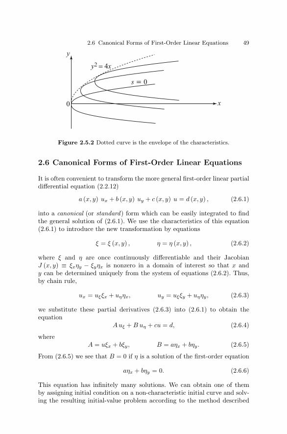
2.6 Canonical Forms of First-Order Linear Equations 49
Figure 2.5.2 Dotted curve is the envelope of the characteristics.
2.6 Canonical Forms of First-Order Linear Equations
It is often convenient to transform the more general first-order linear partialdifferential equation (2.2.12)
a (x, y) ux + b (x, y) uy + c (x, y) u = d (x, y) , (2.6.1)
into a canonical (or standard) form which can be easily integrated to findthe general solution of (2.6.1). We use the characteristics of this equation(2.6.1) to introduce the new transformation by equations
ξ = ξ (x, y) , η = η (x, y) , (2.6.2)
where ξ and η are once continuously differentiable and their JacobianJ (x, y) ≡ ξxηy − ξyηx is nonzero in a domain of interest so that x andy can be determined uniquely from the system of equations (2.6.2). Thus,by chain rule,
ux = uξξx + uηηx, uy = uξξy + uηηy, (2.6.3)
we substitute these partial derivatives (2.6.3) into (2.6.1) to obtain theequation
A uξ + B uη + cu = d, (2.6.4)
whereA = uξx + bξy, B = aηx + bηy. (2.6.5)
From (2.6.5) we see that B = 0 if η is a solution of the first-order equation
aηx + bηy = 0. (2.6.6)
This equation has infinitely many solutions. We can obtain one of themby assigning initial condition on a non-characteristic initial curve and solv-ing the resulting initial-value problem according to the method described

50 2 First-Order, Quasi-Linear Equations and Method of Characteristics
earlier. Since η (x, y) satisfies equation (2.6.6), the level curves η (x, y) =constant are always characteristic curves of equation (2.6.1). Thus, one setof the new transformations are the characteristic curves of (2.6.1). The sec-ond set, ξ (x, y) = constant, can be chosen to be any one parameter familyof smooth curves which are nowhere tangent to the family of the character-istic curves. We next assert that A = 0 in a neighborhood of some point inthe domain D in which η (x, y) is defined and J = 0. For, if A = 0 at somepoint of D, then B = 0 at the same point. Consequently, equations (2.6.5)would form a system of linear homogeneous equations in a and b, where theJacobian J is the determinant of its coefficient matrix. Since J = 0, both aand b must be zero at that point which contradicts the original assumptionthat a and b do not vanish simultaneously. Finally, since B = 0 and A = 0in D, we can divide (2.6.4) by A to obtain the canonical form
uξ + α (ξ, η) u = β (ξ, η) , (2.6.7)
where α (ξ, η) = cA and β (ξ, η) = d
A .Equation (2.6.7) represents an ordinary differential equation with ξ as
the independent variable and η as a parameter which may be treated asconstant. This equation (2.6.7) is called the canonical form of equation(2.6.1) in terms of the coordinates (ξ, η). Generally, the canonical equation(2.6.7) can easily be integrated and the general solution of (2.6.1) can beobtained after replacing ξ and η by the original variables x and y.
We close this section by considering some examples that illustrate thisprocedure. In practice, it is convenient to choose ξ = ξ (x, y) and η (x, y) = yor ξ = x and η = η (x, y) so that J = 0.
Example 2.6.1. Reduce each of the following equations
ux − uy = u, (2.6.8)yux + uy = x, (2.6.9)
to canonical form, and obtain the general solution.
In (2.6.8), a = 1, b = −1, c = −1 and d = 0. The characteristic equationsare
dx
1=
dy
−1=
du
u.
The characteristic curves are ξ = x + y = c1, and we choose η = y = c2where c1 and c2 are constants. Consequently, ux = uξ and uy = uξ + uη,and hence, equation (2.6.8) becomes
uη = u.
Integrating this equation gives

2.7 Method of Separation of Variables 51
ln u (ξ, η) = −η + ln f (ξ) ,
where f (ξ) is an arbitrary function of ξ only.Equivalently,
u (ξ, η) = f (ξ) e−η.
In terms of the original variables x and y, the general solution of equa-tion (2.6.8) is
u (x, y) = f (x + y) e−y, (2.6.10)
where f is an arbitrary function.The characteristic equations of (2.6.9) are
dx
y=
dy
1=
du
x.
It follows from the first two equations that ξ (x, y) = x− y2
2 = c1; we chooseη (x, y) = y = c2. Consequently, ux = uξ and uy = −y uξ + uη and hence,equation (2.6.9) reduces to
uη = ξ +12η2.
Integrating this equation gives the general solution
u (ξ, η) = ξη +16η3 + f (ξ) ,
where f is an arbitrary function.Thus, the general solution of (2.6.9) in terms of x and y is
u (x, y) = xy − 13y3 + f
(x − y2
2
).
2.7 Method of Separation of Variables
During the last two centuries several methods have been developed for solv-ing partial differential equations. Among these, a technique known as themethod of separation of variables is perhaps the oldest systematic methodfor solving partial differential equations. Its essential feature is to transformthe partial differential equations by a set of ordinary differential equations.The required solution of the partial differential equations is then exposed asa product u (x, y) = X (x) Y (y) = 0, or as a sum u (x, y) = X (x) + Y (y),where X (x) and Y (y) are functions of x and y, respectively. Many signifi-cant problems in partial differential equations can be solved by the method

52 2 First-Order, Quasi-Linear Equations and Method of Characteristics
of separation of variables. This method has been considerably refined andgeneralized over the last two centuries and is one of the classical techniquesof applied mathematics, mathematical physics and engineering science.
Usually, the first-order partial differential equation can be solved by sep-aration of variables without the need for Fourier series. The main purposeof this section is to illustrate the method by examples.
Example 2.7.1. Solve the initial-value problem
ux + 2uy = 0, u (0, y) = 4 e−2y. (2.7.1ab)
We seek a separable solution u (x, y) = X (x) Y (y) = 0 and substituteinto the equation to obtain
X ′ (x) Y (y) + 2X (x) Y ′ (y) = 0.
This can also be expressed in the form
X ′ (x)2X (x)
= −Y ′ (y)Y (y)
. (2.7.2)
Since the left-hand side of this equation is a function of x only and theright-hand is a function of y only, it follows that (2.7.2) can be true if bothsides are equal to the same constant value λ which is called an arbitraryseparation constant. Consequently, (2.7.2) gives two ordinary differentialequations
X ′ (x) − 2λX (x) = 0, Y ′ (y) + λY (y) = 0. (2.7.3)
These equations have solutions given, respectively, by
X (x) = A e2λx and Y (y) = B e−λy, (2.7.4)
where A and B are arbitrary integrating constants.Consequently, the general solution is given by
u (x, y) = AB exp (2λx − λy) = C exp (2λx − λy) , (2.7.5)
where C = AB is an arbitrary constant.Using the condition (2.7.1b), we find
4 e−2y = u (0, y) = Ce−λy,
and hence, we deduce that C = 4 and λ = 2. Therefore, the final solutionis
u (x, y) = 4 exp (4x − 2y) . (2.7.6)

2.7 Method of Separation of Variables 53
Example 2.7.2. Solve the equation
y2u2x + x2u2
y = (xyu)2 . (2.7.7)
We assume u (x, y) = f (x) g (y) = 0 is a separable solution of (2.7.7),and substitute into the equation. Consequently, we obtain
y2 f ′ (x) g (y)2 + x2 f (x) g′ (y)2 = x2y2 f (x) g (y)2,
or, equivalently,
1x2
f ′ (x)f (x)
2
+1y2
g′ (y)g (y)
2
= 1,
or
1x2
f ′ (x)f (x)
2
= 1 − 1y2
g′ (y)g (y)
2
= λ2,
where λ2 is a separation constant. Thus,
1x
f ′ (x)f (x)
= λ andg′ (y)y g (y)
=√
1 − λ2 . (2.7.8)
Solving these ordinary differential equations, we find
f (x) = A exp(
λ
2x2
)and g (y) = B exp
(12
y√
1 − λ2
),
where A and B are arbitrary constant. Thus, the general solution is
u (x, y) = C exp(
λ
2x2 +
12y2
√1 − λ2
), (2.7.9)
where C = AB is an arbitrary constant.Using the condition u (x, 0) = 3 exp
(x2/4
), we can determine both C
and λ in (2.7.9). It turns out that C = 3 and λ = (1/2), and the solutionbecomes
u (x, y) = 3 exp[14
(x2 + y2
√3)]
. (2.7.10)
Example 2.7.3. Use the separation of variables u (x, y) = f (x) + g (y) tosolve the equation
u2x + u2
y = 1. (2.7.11)
Obviously,

54 2 First-Order, Quasi-Linear Equations and Method of Characteristics
f ′ (x)2 = 1 − g′ (y)2 = λ2,
where λ2 is a separation constant. Thus, we obtain
f ′ (x) = λ and g′ (y) =√
1 − λ2 .
Solving these ordinary differential equations, we find
f (x) = λx + A and g (y) = y√
1 − λ2 + B,
where A and B are constants of integration. Finally, the solution of (2.7.11)is given by
u (x, y) = λx + y√
1 − λ2 + C, (2.7.12)
where C = A + B is an arbitrary constant.
Example 2.7.4. Use u (x, y) = f (x) + g (y) to solve the equation
u2x + uy + x2 = 0. (2.7.13)
Obviously, equation (2.7.13) has the separable form
f ′ (x)2 + x2 = −g′ (y) = λ2,
where λ2 is a separation constant.Consequently,
f ′ (x) =√
λ2 − x2 and g′ (y) = −λ2.
These can be integrated to obtain
f (x) =∫ √
λ2 − x2 dx + A
= λ2∫
cos2 θ dθ + A, (x = λ sin θ)
=12λ2
[sin−1
(x
λ
)+
x
λ
√1 − x2
λ2
]+ A
and
g (y) = −λ2y + B.
Finally, the general solution is given by
u (x, y) =12λ2 sin−1
(x
λ
)+
x
2
√λ2 − x2 − λ2y + C, (2.7.14)
where C = A + B is an arbitrary constant.
2.8 Exercises 55
Example 2.7.5. Use v = lnu and v = f (x) + g (y) to solve the equation
x2u2x + y2u2
y = u2. (2.7.15)
In view of v = lnu, vx = 1uux and vy = 1
uuy, and hence, equation (2.7.15)becomes
x2v2x + y2v2
y = 1. (2.7.16)
Substitute v (x, y) = f (x) + g (y) into (2.7.16) to obtain
x2 f ′ (x)2 + y2 g′ (y)2 = 1
or
x2 f ′ (x)2 = 1 − y2 g′ (y)2 = λ2,
where λ2 is a separation constant. Thus, we obtain
f ′ (x) =λ
xand g′ (y) =
1y
√1 − λ2 .
Integrating these equations gives
f (x) = λ lnx + A and g (y) =√
1 − λ2 ln y + B,
where A and B are integrating constants. Therefore, the general solutionof (2.7.16) is given by
v (x, y) = λ lnx +√
1 − λ2 ln y + lnC
= ln(xλ · y
√1−λ2 · C
), (2.7.17)
where ln C = A + B. The final solution is
u (x, y) = ev = C xλ · y√
1−λ2, (2.7.18)
where C is an integrating constant.
2.8 Exercises
1. (a) Show that the family of right circular cones whose axes coincidewith the z-axis
x2 + y2 = (z − c)2 tan2 α
satisfies the first-order, partial differential equation

56 2 First-Order, Quasi-Linear Equations and Method of Characteristics
yp − xq = 0.
(b) Show that all the surfaces of revolution, z = f(x2 + y2
)with the
z-axis as the axis of symmetry, where f is an arbitrary function, satisfythe partial differential equation
yp − xq = 0.
(c) Show that the two-parameter family of curves u − ax − by − ab = 0satisfies the nonlinear equation
xp + yq + pq = u.
2. Find the partial differential equation arising from each of the followingsurfaces:
(a) z = x + y + f (xy), (b) z = f (x − y),
(c) z = xy + f(x2 + y2
), (d) 2z = (αx + y)2 + β.
3. Find the general solution of each of the following equations:
(a) ux = 0, (b) a ux + b uy = 0; a, b, are constant,
(c) ux + y uy = 0, (d)(1 + x2
)ux + uy = 0,
(e) 2xy ux +(x2 + y2
)uy = 0, (f) (y + u) ux + y uy = x − y,
(g) y2ux − xy uy = x (u − 2y), (h) yuy − xux = 1,
(i) y2up + u2xq = −xy2, (j) (y − xu) p + (x + yu) q = x2 + y2.
4. Find the general solution of the equation
ux + 2xy2uy = 0.
5. Find the solution of the following Cauchy problems:
(a) 3ux + 2uy = 0, with u (x, 0) = sinx,
(b) y ux + x uy = 0, with u (0, y) = exp(−y2
),
(c) x ux + y uy = 2xy, with u = 2 on y = x2,
(d) ux + x uy = 0, with u (0, y) = sin y,
(e) y ux + x uy = xy, x ≥ 0, y ≥ 0, with u (0, y) = exp(−y2
)for y > 0, and u (x, 0) = exp
(−x2)
for x > 0,
2.8 Exercises 57
(f) ux + x uy =(y − 1
2x2)2, with u (0, y) = exp (y),
(g) x ux + y uy = u + 1, with u (x, y) = x2 on y = x2,
(h) uux − uuy = u2 + (x + y)2, with u = 1 on y = 0,
(i) x ux + (x + y) uy = u + 1, with u (x, y) = x2 on y = 0.
(j)√
x ux + uuy + u2 = 0, u (x, 0) = 1, 0 < x < ∞.
(k) ux2ux + e−yuy + u2 = 0, u (x, 0) = 1, 0 < x < ∞.
6. Solve the initial-value problem
ut + uux = 0
with the initial curve
x =12τ2, t = τ, u = τ.
7. Find the solution of the Cauchy problem
2xy ux +(x2 + y2)uy = 0, with u = exp
(x
x − y
)onx + y = 1.
8. Solve the following equations:
(a) x ux + y uy + z uz = 0,
(b) x2 ux + y2 uy + z (x + y) uz = 0,
(c) x (y − z) ux + y (z − x) uy + z (x − y) uz = 0,
(d) yz ux − xz uy + xy(x2 + y2
)uz = 0,
(e) x(y2 − z2
)ux + y
(z2 − y2
)uy + z
(x2 − y2
)uz = 0.
9. Solve the equation
ux + x uy = y
with the Cauchy data
(a) u (0, y) = y2, (b) u (1, y) = 2y.
58 2 First-Order, Quasi-Linear Equations and Method of Characteristics
10. Show that u1 = ex and u2 = e−y are solutions of the nonlinear equation
(ux + uy)2 − u2 = 0
but that their sum (ex + e−y) is not a solution of the equation.
11. Solve the Cauchy problem
(y + u) ux + y uy = (x − y) , with u = 1 + x on y = 1.
12. Find the integral surfaces of the equation uux + uy = 1 for each of thefollowing initial data:
(a) x (s, 0) = s, y (s, 0) = 2s, u (s, 0) = s,
(b) x (s, 0) = s2, y (s, 0) = 2s, u (s, 0) = s,
(c) x (s, 0) = s2
2 , y (s, 0) = s, u (s, 0) = s.
Draw characteristics in each case.13. Show that the solution of the equation
y ux − x uy = 0
containing the curve x2 + y2 = a2, u = y, does not exist.
14. Solve the following Cauchy problems:
(a) x2ux − y2uy = 0, u → ex as y → ∞,
(b) y ux + x uy = 0, u = sinx on x2 + y2 = 1,
(c) −x ux + y uy = 1 for 0 < x < y, u = 2x on y = 3x,
(d) 2x ux + (x + 1)uy = y for x > 0, u = 2y on x = 1,
(e) x ux − 2y uy = x2 + y2 for x > 0, y > 0, u = x2 on y = 1,
(f) ux + 2 uy = 1 + u, u (x, y) = sinx on y = 3x + 1,
(g) ux + 3uy = u, u (x, y) = cos x on y = x,
(h) ux + 2x uy = 2xu, u (x, 0) = x2,
(i) uux + uy = u, u (x, 0) = 2x, 1 ≤ x ≤ 2,
(j) ux + uy = u2, u (x, 0) = tanhx.

2.8 Exercises 59
Show that the solution of (j) is unbounded on the critical curvey tanh (x − y) = 1.
15. Find the solution surface of the equation(u2 − y2)ux + xy uy + xu = 0, with u = y = x, x > 0.
16. (a) Solve the Cauchy problem
ux + uuy = 1, u (0, y) = ay,
where a is a constant.(b) Find the solution of the equation in (a) with the data
x (s, 0) = 2s, y (s, 0) = s2, u(0, s2) = s.
17. Solve the following equations:
(a) (y + u) ux + (x + u) uy = x + y,
(b) x u(u2 + xy
)ux − y u
(u2 + xy
)uy = x4,
(c) (x + y) ux + (x − y) uy = 0,
(d) y ux + x uy = xy(x2 − y2
),
(e) (cy − bz) zx + (az − cx) zy = bx − ay.
18. Solve the equation
x zx + y zy = z,
and find the curves which satisfy the associated characteristic equationsand intersect the helix x + y2 = a2, z = b tan−1
(yx
).
19. Obtain the family of curves which represent the general solution of thepartial differential equation
(2x − 4y + 3u) ux + (x − 2y − 3u) uy = −3 (x − 2y) .
Determine the particular member of the family which contains the lineu = x and y = 0.
20. Find the solution of the equation
y ux − 2xy uy = 2xu
with the condition u (0, y) = y3.

60 2 First-Order, Quasi-Linear Equations and Method of Characteristics
21. Obtain the general solution of the equation
(x + y + 5z) p + 4zq + (x + y + z) = 0 (p = zx, q = zy) ,
and find the particular solution which passes through the circle
z = 0, x2 + y2 = a2.
22. Obtain the general solution of the equation(z2 − 2yz − y2) p + x (y + z) q = x (y − z) (p = zx, q = zy) .
Find the integral surfaces of this equation passing through
(a) the x-axis, (b) the y-axis, and (c) the z-axis.
23. Solve the Cauchy problem
(x + y) ux + (x − y) uy = 1, u (1, y) =1√2.
24. Solve the following Cauchy problems:
(a) 3 ux + 2 uy = 0, u (x, 0) = f (x),
(b) a ux + b uy = c u, u (x, 0) = f (x), where a, b, c are constants,
(c) x ux + y uy = c u, u (x, 0) = f (x),
(d) uux + uy = 1, u (s, 0) = αs, x (s, 0) = s, y (s, 0) = 0.
25. Apply the method of separation of variables u (x, y) = f (x) g (y) tosolve the following equations:
(a) ux + u = uy, u (x, 0) = 4e−3x, (b) uxuy = u2,
(c) ux + 2uy = 0, u (0, y) = 3e−2y, (d) y2u2x + x2u2
y = (xyu)2,
(e) x2uxy + 9y2u = 0, u (x, 0) = exp( 1
x
), (f) y ux − x uy = 0,
(g) ut = c2 (uxx + uyy), (h) uxx + uyy = 0.
26. Use a separable solution u (x, y) = f (x) + g (y) to solve the followingequations:
(a) u2x + u2
y = 1, (b) u2x + u2
y = u,
(c) u2x + uy + x2 = 0, (d) x2u2
x + y2u2y = 1,
(e) y ux + x uy = 0, u (0, y) = y2.

2.8 Exercises 61
27. Apply v = lnu and then v (x, y) = f (x) + g (y) to solve the followingequations:
(a) x2u2x + y2u2
y = u2,
(b) x2u2x + y2u2
y = (xyu)2.
28. Apply√
u = v and v (x, y) = f (x) + g (y) to solve the equation
x4u2x + y2u2
y = 4u.
29. Using v = lnu and v = f (x) + g (y), show that the solution of theCauchy problem
y2u2x + x2u2
y = (xyu)2 , u (x, 0) = ex2
is
u (x, y) = exp
(x2 + i
√3
2y2
).
30. Reduce each of the following equations into canonical form and find thegeneral solution:
(a) ux + uy = u, (b) ux + x uy = y,
(c) ux + 2xy uy = x, (d) ux − y uy − u = 1.
31. Find the solution of each of the following equations by the method ofseparation of variables:
(a) ux − uy = 0, u (0, y) = 2e3y,
(b) ux − uy = u, u (x, 0) = 4e−3x,
(c) a ux + b uy = 0, u (x, 0) = αeβx,
where a, b, α and β are constants.
32. Find the solution of the following initial-value systems
(a) ut + 3uux = v − x, vt − cvx = 0 with u (x, 0) = x and v (x, 0) = x.
(b) ut + 2uux = v − x, vt − cvx = 0 with u (x, 0) = x and v (x, 0) = x.

62 2 First-Order, Quasi-Linear Equations and Method of Characteristics
33. Solve the following initial-value systems
(a) ut + uux = e−xv, vt − avx = 0 with u (x, 0) = x and v (x, 0) = ex.
(b) ut − 2uux = v − x, vt + cvx = 0 with u (x, 0) = x and v (x, 0) = x.
34. Consider the Fokker–Planck equation (See Reif (1965)) in statistical me-chanics to describe the evolution of the probability distribution functionin the form
ut = uxx + (x u)x ,
u (x, 0) = f (x) .
Neglecting the term uxx, solve the first-order linear equation
ut − x ux = u with u (x, 0) = f (x) .

3
Mathematical Models
“Physics can’t exist without mathematics which provides it with the onlylanguage in which it can speak. Thus, services are continuously exchangedbetween pure mathematical analysis and physics. It is really remarkablethat among works of analysis most useful for physics were those cultivatedfor their own beauty. In exchange, physics, exposing new problems, is asuseful for mathematics as it is a model for an artist.”
Henri Poincare
“It is no paradox to say in our most theoretical models we may be nearestto our most practical applications.”
A. N. Whitehead
“... builds models based on data from all levels: gene expression, proteinlocation in the cell, models of cell function, and computer representationsof organs and organisms.”
E. Pennisi
3.1 Classical Equations
Partial differential equations arise frequently in formulating fundamentallaws of nature and in the study of a wide variety of physical, chemical,and biological models. We start with a special type of second-order linearpartial differential equation for the following reasons. First, second-orderlinear equations arise more frequently in a wide variety of applications.Second, their mathematical treatment is simpler and easier to understandthan that of first-order equations in general. Usually, in almost all physical

64 3 Mathematical Models
phenomena (or physical processes), the dependent variable u = u (x, y, z, t)is a function of three space variables, x, y, z and time variable t.
The three basic types of second-order partial differential equations are:(a) The wave equation
utt − c2 (uxx + uyy + uzz) = 0. (3.1.1)
(b) The heat equation
ut − k (uxx + uyy + uzz) = 0. (3.1.2)
(c) The Laplace equation
uxx + uyy + uzz = 0. (3.1.3)
In this section, we list a few more common linear partial differential equa-tions of importance in applied mathematics, mathematical physics, and en-gineering science. Such a list naturally cannot ever be complete. Includedare only equations of most common interest:
(d) The Poisson equation
∇2u = f (x, y, z) . (3.1.4)
(e) The Helmholtz equation
∇2u + λu = 0. (3.1.5)
(f) The biharmonic equation
∇4u = ∇2 (∇2u)
= 0. (3.1.6)
(g) The biharmonic wave equation
utt + c2∇4u = 0. (3.1.7)
(h) The telegraph equation
utt + aut + bu = c2uxx. (3.1.8)
(i) The Schrodinger equations in quantum physics
iψt =[(
− 2
2m
)∇2 + V (x, y, z)
]ψ, (3.1.9)
∇2Ψ +2m
2 [E − V (x, y, z)] Ψ = 0. (3.1.10)
(j) The Klein–Gordon equation
u + λ2u = 0, (3.1.11)

3.2 The Vibrating String 65
where
∇2 ≡ ∂2
∂x2 +∂2
∂y2 +∂2
∂z2 , (3.1.12)
is the Laplace operator in rectangular Cartesian coordinates (x, y, z),
≡ ∇2 − 1c2
∂2
∂t2, (3.1.13)
is the d’Alembertian, and in all equations λ, a, b, c, m, E are constantsand h = 2π is the Planck constant.(k) For a compressible fluid flow, Euler’s equations
ut + (u · ∇)u = −1ρ∇p, ρt + div (ρu) = 0, (3.1.14)
where u = (u, v, w) is the fluid velocity vector, ρ is the fluid density,and p = p (ρ) is the pressure that relates p and ρ (the constitutiveequation or equation of state).Many problems in mathematical physics reduce to the solving of partial
differential equations, in particular, the partial differential equations listedabove. We will begin our study of these equations by first examining indetail the mathematical models representing physical problems.
3.2 The Vibrating String
One of the most important problems in mathematical physics is the vi-bration of a stretched string. Simplicity and frequent occurrence in manybranches of mathematical physics make it a classic example in the theoryof partial differential equations.
Let us consider a stretched string of length l fixed at the end points. Theproblem here is to determine the equation of motion which characterizesthe position u (x, t) of the string at time t after an initial disturbance isgiven.
In order to obtain a simple equation, we make the following assumptions:
1. The string is flexible and elastic, that is the string cannot resist bendingmoment and thus the tension in the string is always in the direction ofthe tangent to the existing profile of the string.
2. There is no elongation of a single segment of the string and hence, byHooke’s law, the tension is constant.
3. The weight of the string is small compared with the tension in thestring.
4. The deflection is small compared with the length of the string.5. The slope of the displaced string at any point is small compared with
unity.

66 3 Mathematical Models
6. There is only pure transverse vibration.
We consider a differential element of the string. Let T be the tension at theend points as shown in Figure 3.2.1. The forces acting on the element ofthe string in the vertical direction are
T sin β − T sin α.
By Newton’s second law of motion, the resultant force is equal to themass times the acceleration. Hence,
T sin β − T sin α = ρ δs utt (3.2.1)
where ρ is the line density and δs is the smaller arc length of the string.Since the slope of the displaced string is small, we have
δs δx.
Since the angles α and β are small
sin α tanα, sin β tanβ.
Figure 3.2.1 An Element of a vertically displaced string.

3.3 The Vibrating Membrane 67
Thus, equation (3.2.1) becomes
tanβ − tanα =ρ δx
Tutt. (3.2.2)
But, from calculus we know that tan α and tanβ are the slopes of the stringat x and x + δx:
tanα = ux (x, t)
and
tanβ = ux (x + δx, t)
at time t. Equation (3.2.2) may thus be written as
1δx
[(ux)x+δx − (ux)x
]=
ρ
Tutt,
1δx
[ux (x + δx, t) − ux (x, t)] =ρ
Tutt.
In the limit as δx approaches zero, we find
utt = c2uxx (3.2.3)
where c2 = T/ρ. This is called the one-dimensional wave equation.If there is an external force f per unit length acting on the string.
Equation (3.2.3) assumes the form
utt = c2uxx + F, F = f/ρ, (3.2.4)
where f may be pressure, gravitation, resistance, and so on.
3.3 The Vibrating Membrane
The equation of the vibrating membrane occurs in a large number of prob-lems in applied mathematics and mathematical physics. Before we derivethe equation for the vibrating membrane we make certain simplifying as-sumptions as in the case of the vibrating string:
1. The membrane is flexible and elastic, that is, the membrane cannotresist bending moment and the tension in the membrane is always inthe direction of the tangent to the existing profile of the membrane.
2. There is no elongation of a single segment of the membrane and hence,by Hooke’s law, the tension is constant.
3. The weight of the membrane is small compared with the tension in themembrane.
4. The deflection is small compared with the minimal diameter of themembrane.

68 3 Mathematical Models
5. The slope of the displayed membrane at any point is small comparedwith unity.
6. There is only pure transverse vibration.
We consider a small element of the membrane. Since the deflection andslope are small, the area of the element is approximately equal to δxδy. IfT is the tensile force per unit length, then the forces acting on the sides ofthe element are T δx and T δy, as shown in Figure 3.3.1.
The forces acting on the element of the membrane in the vertical direc-tion are
T δx sin β − T δx sin α + T δy sin δ − T δy sin γ.
Since the slopes are small, sines of the angles are approximately equal totheir tangents. Thus, the resultant force becomes
T δx (tanβ − tanα) + T δy (tan δ − tan γ) .
By Newton’s second law of motion, the resultant force is equal to themass times the acceleration. Hence,
T δx (tanβ − tanα) + T δy (tan δ − tan γ) = ρ δA utt (3.3.1)
where ρ is the mass per unit area, δA δxδy is the area of this element,and utt is computed at some point in the region under consideration. Butfrom calculus, we have
Figure 3.3.1 An element of vertically displaced membrane.

3.4 Waves in an Elastic Medium 69
tanα = uy (x1, y)tanβ = uy (x2, y + δy)tan γ = ux (x, y1)tan δ = ux (x + δx, y2)
where x1 and x2 are the values of x between x and x+δx, and y1 and y2 arethe values of y between y and y + δy. Substituting these values in (3.3.1),we obtain
T δx [uy (x2, y + δy) − uy (x1, y)] + T δy [ux (x + δx, y2) − ux (x, y1)]= ρ δxδy utt.
Division by ρ δxδy yields
T
ρ
[uy (x2, y + δy) − uy (x1, y)
δy+
ux (x + δx, y2) − ux (x, y1)δx
]= utt.
(3.3.2)
In the limit as δx approaches zero and δy approaches zero, we obtain
utt = c2 (uxx + uyy) , (3.3.3)
where c2 = T/ρ. This equation is called the two-dimensional wave equation.If there is an external force f per unit area acting on the membrane.
Equation (3.3.3) takes the form
utt = c2 (uxx + uyy) + F, (3.3.4)
where F = f/ρ.
3.4 Waves in an Elastic Medium
If a small disturbance is originated at a point in an elastic medium, neigh-boring particles are set into motion, and the medium is put under a stateof strain. We consider such states of motion to extend in all directions. Weassume that the displacements of the medium are small and that we arenot concerned with translation or rotation of the medium as a whole.
Let the body under investigation be homogeneous and isotropic. Let δVbe a differential volume of the body, and let the stresses acting on the facesof the volume be τxx, τyy, τzz, τxy, τxz, τyx, τyz, τzx, τzy. The first threestresses are called the normal stresses and the rest are called the shearstresses. (See Figure 3.4.1).
We shall assume that the stress tensor τij is symmetric describing thecondition of the rotational equilibrium of the volume element, that is,

70 3 Mathematical Models
Figure 3.4.1 Volume element of an elastic body.
τij = τji, i = j, i, j = x, y, z. (3.4.1)
Neglecting the body forces, the sum of all the forces acting on the volumeelement in the x-direction is[
(τxx)x+δx − (τxx)x
]δyδz +
[(τxy)y+δy − (τxy)y
]δzδx
+[(τxz)z+δz − (τxz)z
]δxδy.
By Newton’s law of motion this resultant force is equal to the mass timesthe acceleration. Thus, we obtain[
(τxx)x+δx − (τxx)x
]δyδz +
[(τxy)y+δy − (τxy)y
]δzδx
+[(τxz)z+δz − (τxz)z
]δxδy = ρ δxδyδz utt (3.4.2)
where ρ is the density of the body and u is the displacement component inthe x-direction. Hence, in the limit as δV approaches zero, we obtain
∂τxx
∂x+
∂τxy
∂y+
∂τxz
∂z= ρ
∂2u
∂t2. (3.4.3)
Similarly, the following two equations corresponding to y and z directionsare obtained:

3.4 Waves in an Elastic Medium 71
∂τyx
∂x+
∂τyy
∂y+
∂τyz
∂z= ρ
∂2v
∂t2, (3.4.4)
∂τzx
∂x+
∂τzy
∂y+
∂τzz
∂z= ρ
∂2w
∂t2, (3.4.5)
where v and w are the displacement components in the y and z directionsrespectively.
We may now define linear strains [see Sokolnikoff (1956)] as
εxx =∂u
∂x, εyz =
12
(∂w
∂y+
∂v
∂z
),
εyy =∂v
∂y, εzx =
12
(∂u
∂z+
∂w
∂x
), (3.4.6)
εzz =∂w
∂z, εxy =
12
(∂v
∂x+
∂u
∂y
),
in which εxx, εyy, εzz represent unit elongations and εyz, εzx, εxy representunit shearing strains.
In the case of an isotropic body, generalized Hooke’s law takes the form
τxx = λθ + 2µεxx, τyz = 2µεyz,
τyy = λθ + 2µεyy, τzx = 2µεzx, (3.4.7)τzz = λθ + 2µεzz, τxy = 2µεxy,
where θ = εxx + εyy + εzz is called the dilatation, and λ and µ are Lame’sconstants.
Expressing stresses in terms of displacements, we obtain
τxx = λθ + 2µ∂u
∂x,
τxy = µ
(∂v
∂x+
∂u
∂y
), (3.4.8)
τxz = µ
(∂w
∂x+
∂u
∂z
).
By differentiating equations (3.4.8), we obtain
∂τxx
∂x= λ
∂θ
∂x+ 2µ
∂2u
∂x2 ,
∂τxy
∂y= µ
∂2v
∂x∂y+ µ
∂2u
∂y2 , (3.4.9)
∂τxz
∂z= µ
∂2w
∂x∂z+ µ
∂2u
∂z2 .
Substituting equation (3.4.9) into equation (3.4.3) yields

72 3 Mathematical Models
λ∂θ
∂x+ µ
(∂2u
∂x2 +∂2v
∂x∂y+
∂2w
∂x∂z
)+ µ
(∂2u
∂x2 +∂2u
∂y2 +∂2u
∂z2
)= ρ
∂2u
∂t2.
(3.4.10)
We note that
∂2u
∂x2 +∂2v
∂x∂y+
∂2w
∂x∂z=
∂
∂x
(∂u
∂x+
∂v
∂y+
∂w
∂z
)=
∂θ
∂x,
and introduce the notation
= ∇2 =∂2
∂x2 +∂2
∂y2 +∂2
∂z2 .
The symbol or ∇2 is called the Laplace operator. Hence, equation (3.4.10)becomes
(λ + µ)∂θ
∂x+ µ∇2u = ρ
∂2u
∂t2. (3.4.11)
In a similar manner, we obtain the other two equations which are
(λ + µ)∂θ
∂y+ µ∇2v = ρ
∂2v
∂t2. (3.4.12)
(λ + µ)∂θ
∂z+ µ∇2w = ρ
∂2w
∂t2. (3.4.13)
The set of equations (3.4.11)–(3.4.13) is called the Navier equations of mo-tion. In vector form, the Navier equations of motion assume the form
(λ + µ) grad divu + µ∇2u = ρutt, (3.4.14)
where u = ui + vj + wk and θ = divu.(i) If divu = 0, the general equation becomes
µ∇2u = ρutt,
or
utt = c2T ∇2u, (3.4.15)
where cT is called the transverse wave velocity given by
cT =√
µ/ρ.
This is the case of an equivoluminal wave propagation, since the volumeexpansion θ is zero for waves moving with this velocity. Sometimes thesewaves are called waves of distortion because the velocity of propagationdepends on µ and ρ; the shear modulus µ characterizes the distortion androtation of the volume element.

3.4 Waves in an Elastic Medium 73
(ii) When curl u = 0, the vector identity
curl curlu = grad divu − ∇2u,
gives
grad divu = ∇2u,
Then the general equation becomes
(λ + 2µ) ∇2u = ρutt,
or
utt = c2L∇2u, (3.4.16)
where cL is called the longitudinal wave velocity given by
cL =
√λ + 2µ
ρ.
This is the case of irrotational or dilatational wave propagation, sincecurlu = 0 describes irrotational motion. Equations (3.4.15) and (3.4.16)are called the three-dimensional wave equations.
In general, the wave equation may be written as
utt = c2∇2u, (3.4.17)
where the Laplace operator may be one, two, or three dimensional. Theimportance of the wave equation stems from the facts that this type ofequation arises in many physical problems; for example, sound waves inspace, electrical vibration in a conductor, torsional oscillation of a rod,shallow water waves, linearized supersonic flow in a gas, waves in an elec-tric transmission line, waves in magnetohydrodynamics, and longitudinalvibrations of a bar.
To give a more general method of decomposing elastic waves into trans-verse and longitudinal wave forms, we write the Navier equations of motionin the form
c2T ∇2u +
(c2L − c2
T
)grad (div u) = utt. (3.4.18)
We now decompose this equation into two vector equations by definingu = uT + uL, where uT and uL satisfy the equations
div uT = 0 and curl uL = 0. (3.4.19ab)
Since uT is defined by (3.4.19a) that is divergenceless, it follows from vectoranalysis that there exists a rotation vector ψψψ such that

74 3 Mathematical Models
uT = curl ψψψ, (3.4.20)
where ψψψ is called the vector potential.On the other hand, uL is irrotational as given by (3.4.19b), so there
exists a scalar function φ (x, t), called the scalar potential such that
uL = grad φ. (3.4.21)
Using (3.4.20) and (3.4.21), we can write
u = curl ψψψ + grad φ. (3.4.22)
This means that the displacement vector field is decomposed into a diver-genceless vector and irrotational vector.
Inserting u = uT +uL into (3.4.18), taking the divergence of each termof the resulting equation, and then using (3.4.19a) gives
div[c2L∇2uL − (uL)tt
]= 0. (3.4.23)
It is noted that the curl of the square bracket in (3.4.23) is also zero.Clearly, any vector whose divergence and curl both vanish is identically azero vector. Consequently,
c2L∇2uL = (uL)tt . (3.4.24)
This shows that uL satisfies the vector wave equation with the wave velocitycL. Since uL = grad φ, it is clear that the scalar potential φ also satisfies thewave equation with the same wave speed. All solutions of (3.4.24) representlongitudinal waves that are irrotational (since ψψψ = 0).
Similarly, we substitute u = uL + uT into (3.4.18), take the curl of theresulting equation, and use the fact that curl uL = 0 to obtain
curl[c2T ∇2uT − (uT )tt
]= 0. (3.4.25)
Since the divergence of the expression inside the square bracket is also zero,it follows that
c2T ∇2uT = (uT )tt . (3.4.26)
This is a vector wave equation for uT whose solutions represent transversewaves that are irrotational but are accompanied by no change in volume(equivoluminal, transverse, rotational waves). These waves propagate witha wave velocity cT .
We close this section by seeking time-harmonic solutions of (3.4.18) inthe form
u = Re[U (x, y, z) eiωt
]. (3.4.27)

3.5 Conduction of Heat in Solids 75
Invoking (3.4.27) into equation (3.4.18) gives the following equation forthe function U
cT ∇2U + (cL − cT ) grad (div U) + ω2U = 0. (3.4.28)
Inserting, u = uT + uL, and using the above method of taking thedivergence and curl of (3.4.28) respectively leads to equation for UL andUT as follows
∇2UL + k2L ∇2UL = 0, ∇2UT + k2
T UT = 0, (3.4.29)
where
k2L =
ω2
c2L
and k2T =
ω2
c2T
. (3.4.30)
Equations (3.4.29) are called the reduced wave equations (or the Helmholtzequations) for UL and UT . Obviously, equations (3.4.29) can also be de-rived by assuming time-harmonic solutions for uL and uT in the form⎛⎝uL
uT
⎞⎠ = eiωt
⎛⎝UL
UT
⎞⎠ , (3.4.31)
and substituting these results into (3.4.24) and (3.4.26) respectively.
3.5 Conduction of Heat in Solids
We consider a domain D∗ bounded by a closed surface B∗. Let u (x, y, z, t)be the temperature at a point (x, y, z) at time t. If the temperature is notconstant, heat flows from places of higher temperature to places of lowertemperature. Fourier’s law states that the rate of flow is proportional tothe gradient of the temperature. Thus the velocity of the heat flow in anisotropic body is
v = −Kgradu, (3.5.1)
where K is a constant, called the thermal conductivity of the body.Let D be an arbitrary domain bounded by a closed surface B in D∗.
Then the amount of heat leaving D per unit time is∫∫B
vnds,
where vn = v · n is the component of v in the direction of the outer unitnormal n of B. Thus, by Gauss’ theorem (Divergence theorem)

76 3 Mathematical Models∫∫B
vnds =∫∫∫
D
div (−Kgradu) dx dy dz
= −K
∫∫∫D
∇2u dx dy dz. (3.5.2)
But the amount of heat in D is given by∫∫∫D
σρu dx dy dz, (3.5.3)
where ρ is the density of the material of the body and σ is its specific heat.Assuming that integration and differentiation are interchangeable, the rateof decrease of heat in D is
−∫∫∫
D
σρ∂u
∂tdx dy dz. (3.5.4)
Since the rate of decrease of heat in D must be equal to the amount of heatleaving D per unit time, we have
−∫∫∫
D
σρut dx dy dz = −K
∫∫∫D
∇2u dx dy dz,
or
−∫∫∫
D
[σρut − K∇2u
]dx dy dz = 0, (3.5.5)
for an arbitrary D in D∗. We assume that the integrand is continuous. If wesuppose that the integrand is not zero at a point (x0, y0, z0) in D, then, bycontinuity, the integrand is not zero in a small region surrounding the point(x0, y0, z0). Continuing in this fashion we extend the region encompassingD. Hence the integral must be nonzero. This contradicts (3.5.5). Thus, theintegrand is zero everywhere, that is,
ut = κ∇2u, (3.5.6)
where κ = K/σρ. This is known as the heat equation.This type of equation appears in a great variety of problems in math-
ematical physics, for example the concentration of diffusing material, themotion of a tidal wave in a long channel, transmission in electrical cables,and unsteady boundary layers in viscous fluid flows.
3.6 The Gravitational Potential
In this section, we shall derive one of the most well-known equations in thetheory of partial differential equations, the Laplace equation.

3.6 The Gravitational Potential 77
Figure 3.6.1 Two particles at P and Q.
We consider two particles of masses m and M , at P and Q as shownin Figure 3.6.1. Let r be the distance between them. Then, according toNewton’s law of gravitation, a force proportional to the product of theirmasses, and inversely proportional to the square of the distance betweenthem, is given in the form
F = GmM
r2 , (3.6.1)
where G is the gravitational constant.It is customary in potential theory to choose the unit of force so that
G = 1. Thus, F becomes
F =mM
r2 . (3.6.2)
If r represents the vector PQ, the force per unit mass at Q due to the massat P may be written as
F =−mrr3 = ∇
(m
r
), (3.6.3)
which is called the intensity of the gravitational field of force.We suppose that a particle of unit mass moves under the attraction of
the particle of mass m at P from infinity up to Q. The work done by theforce F is
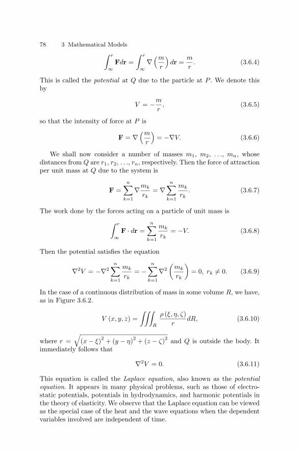
78 3 Mathematical Models∫ r
∞Fdr =
∫ r
∞∇
(m
r
)dr =
m
r. (3.6.4)
This is called the potential at Q due to the particle at P . We denote thisby
V = −m
r, (3.6.5)
so that the intensity of force at P is
F = ∇(m
r
)= −∇V. (3.6.6)
We shall now consider a number of masses m1, m2, . . ., mn, whosedistances from Q are r1, r2, . . ., rn, respectively. Then the force of attractionper unit mass at Q due to the system is
F =n∑
k=1
∇mk
rk= ∇
n∑k=1
mk
rk. (3.6.7)
The work done by the forces acting on a particle of unit mass is∫ r
∞F · dr =
n∑k=1
mk
rk= −V. (3.6.8)
Then the potential satisfies the equation
∇2V = −∇2n∑
k=1
mk
rk= −
n∑k=1
∇2(
mk
rk
)= 0, rk = 0. (3.6.9)
In the case of a continuous distribution of mass in some volume R, we have,as in Figure 3.6.2.
V (x, y, z) =∫∫∫
R
ρ (ξ, η, ζ)r
dR, (3.6.10)
where r =√
(x − ξ)2 + (y − η)2 + (z − ζ)2 and Q is outside the body. Itimmediately follows that
∇2V = 0. (3.6.11)
This equation is called the Laplace equation, also known as the potentialequation. It appears in many physical problems, such as those of electro-static potentials, potentials in hydrodynamics, and harmonic potentials inthe theory of elasticity. We observe that the Laplace equation can be viewedas the special case of the heat and the wave equations when the dependentvariables involved are independent of time.

3.7 Conservation Laws and The Burgers Equation 79
Figure 3.6.2 Continuous Mass Distribution.
3.7 Conservation Laws and The Burgers Equation
A conservation law states that the rate of change of the total amount ofmaterial contained in a fixed domain of volume V is equal to the flux ofthat material across the closed bounding surface S of the domain. If wedenote the density of the material by ρ (x, t) and the flux vector by q (x, t),then the conservation law is given by
d
dt
∫V
ρ dV = −∫
S
(q · n) dS, (3.7.1)
where dV is the volume element and dS is the surface element of the bound-ary surface S, n denotes the outward unit normal vector to S as shown inFigure 3.7.1, and the right-hand side measures the outward flux — hence,the minus sign is used.
Applying the Gauss divergence theorem and taking ddt inside the integral
sign, we obtain ∫V
(∂ρ
∂t+ divq
)dV = 0. (3.7.2)
This result is true for any arbitrary volume V , and, if the integrand iscontinuous, it must vanish everywhere in the domain. Thus, we obtain thedifferential form of the conservation law
ρt + divq = 0. (3.7.3)

80 3 Mathematical Models
Figure 3.7.1 Volume V of a closed domain bounded by a surface S with surfaceelement dS and outward normal vector n.
The one-dimensional version of the conservation law (3.7.3) is
∂ρ
∂t+
∂q
∂x= 0. (3.7.4)
To investigate the nature of the discontinuous solution or shock waves,we assume a functional relation q = Q (ρ) and allow a jump discontinuityfor ρ and q. In many physical problems of interest, it would be a betterapproximation to assume that q is a function of the density gradient ρx aswell as ρ. A simple model is to take
q = Q (ρ) − νρx, (3.7.5)
where ν is a positive constant. Substituting (3.7.5) into (3.7.4), we obtainthe nonlinear diffusion equation
ρt + c (ρ) ρx = νρxx, (3.7.6)
where c (ρ) = Q′ (ρ).We multiply (3.7.6) by c′ (ρ) to obtain
ct + c cx = ν c′ (ρ) ρxx,
= νcxx − c′′ (ρ) ρ2
x
. (3.7.7)
If Q (ρ) is a quadratic function in ρ, then c (ρ) is linear in ρ, and c′′ (ρ) = 0.Consequently, (3.7.7) becomes
ct + c cx = ν cxx. (3.7.8)

3.8 The Schrodinger and the Korteweg–de Vries Equations 81
As a simple model of turbulence, c is replaced by the fluid velocity fieldu (x, t) to obtain the well-known Burgers equation
ut + uux = ν uxx, (3.7.9)
where ν is the kinematic viscosity.Thus the Burgers equation is a balance between time evolution, non-
linearity, and diffusion. This is the simplest nonlinear model equation fordiffusive waves in fluid dynamics. Burgers (1948) first developed this equa-tion primarily to shed light on the study of turbulence described by theinteraction of the two opposite effects of convection and diffusion. However,turbulence is more complex in the sense that it is both three dimensionaland statistically random in nature. Equation (3.7.9) arises in many phys-ical problems including one-dimensional turbulence (where this equationhad its origin), sound waves in a viscous medium, shock waves in a viscousmedium, waves in fluid-filled viscous elastic tubes, and magnetohydrody-namic waves in a medium with finite electrical conductivity. We note that(3.7.9) is parabolic provided the coefficient of ux is constant, whereas theresulting (3.7.9) with ν = 0 is hyperbolic. More importantly, the proper-ties of the solution of the parabolic equation are significantly different fromthose of the hyperbolic equation.
3.8 The Schrodinger and the Korteweg–de VriesEquations
We consider the following Fourier integral representation of a quasi-mono-chromatic plane wave solution
u (x, t) =∫ ∞
−∞F (k) exp [i kx − ω (k) t] dk, (3.8.1)
where the spectrum function F (k) is determined from the given ini-tial or boundary conditions and has the property F (−k) = F ∗ (k), andω = ω (k) is the dispersion relation. We assume that the initial wave isslowly modulated as it propagates in a dispersive medium. For such a quasi-monochromatic wave, most of the energy is confined in a neighborhood ofa specified wave number k = k0, so that spectrum function F (k) has asharp peak around the point k = k0 with a narrow wave number widthk − k0 = δk = O (ε), and the dispersion relation ω (k) can be expandedabout k0 in the form
ω = ω0 + ω′0 (δk) +
12!
ω′′0 (δk)2 +
13!
ω′′′0 (δk)3 + · · · , (3.8.2)
where ω0 = ω (k0), ω′0 = ω′ (k0), ω′′
0 = ω′′ (k0), and ω′′′0 = ω′′′ (k0).

82 3 Mathematical Models
Substituting (3.8.2) into (3.8.1) gives a new form
u (x, t) = A (x, t) exp [i (k0x − ω0t)] + c.c., (3.8.3)
where c.c. stands for the complex conjugate and A (x, t) is the complexwave amplitude given by
A (x, t) =∫ ∞
0F (k0 + δk) exp
[i
(x − ω′
0t) (δk) − 12ω′′
0 (δk)2 t
−13ω′′′
0 (δk)3 t
]d (δk) , (3.8.4)
where it has been assumed that ω (−k) = −ω (k). Since (3.8.4) depends on(x − ω′
0t) δk, (δk)2 t, (δk)3 t where δk = O (ε) is small, the wave amplitudeA (x, t) is a slowly varying function of x∗ = (x − ω′
0t) and time t.We keep only the term with (δk) in (3.8.4) and neglect all terms with
(δk)n, n = 2, 3, · · · , so that (3.8.4) becomes
A (x, t) =∫ ∞
0F (k0 + δk) exp [i (x − ω′
0t) (δk)] d (δk) . (3.8.5)
A simple calculation reveals that A (x, t) satisfies the evolution equation
∂A
∂t+ cg
∂A
∂x= 0, (3.8.6)
where cg = ω′0 is the group velocity.
In the next step, we retain only terms with (δk) and (δk)2 in (3.8.4) toobtain
A (x, t) =∫ ∞
0F (k0 + δk) exp
[i
(x − ω′
0t) (δk) − 12ω′′
0 (δk)2]
d (δk) .
(3.8.7)
A simple calculation shows that A (x, t) satisfies the linear Schrodingerequation
i
(∂A
∂t+ ω′
0∂A
∂x
)+
12
ω′′0
∂2A
∂x2 = 0. (3.8.8)
Using the slow variables
ξ = ε (x − ω′0t) , τ = ε2t, (3.8.9)
the modulated wave amplitude A (ξ, τ) satisfies the linear Schrodinger equa-tion
i Aτ +12ω′′
0Aξξ = 0. (3.8.10)

3.9 Exercises 83
On the other hand, for the frequencies at which the group velocity ω′0
reaches an extremum, ω′′0 = 0. In this case, the cubic term in the dispersion
relation (3.7.2) plays an important role. Consequently, equation (3.8.4) re-duces to a form similar to (3.8.7) with ω′′
0 = 0 in the exponential factor.Once again, a simple calculation from the resulting integral (3.8.4) revealsthat A (x, t) satisfies the linearized Korteweg–de Vries (KdV) equation
∂A
∂t+ ω′
0∂A
∂x+
16
ω′′′0
∂3A
∂x3 = 0. (3.8.11)
By transferring to the new variables ξ = x−ω′0t and τ = t which correspond
to a reference system moving with the group velocity ω′0, we obtain the
linearized KdV equation
∂A
∂τ+
16
ω′′′0
∂3A
∂ξ3 = 0. (3.8.12)
This describes waves in a dispersive medium with a weak high frequencydispersion.
One of the remarkable nonlinear model equations is the Korteweg–deVries (KdV) equation in the form
ut + αuux + βuxxx = 0, −∞ < x < ∞, t > 0. (3.8.13)
This equation arises in many physical problems including water waves, ionacoustic waves in a plasma, and longitudinal dispersive waves in elastic rods.The exact solution of this equation is called the soliton which is remarkablystable. We shall discuss the soliton solution in Chapter 13.
Another remarkable nonlinear model equation describing solitary wavesis known as the nonlinear Schrodinger (NLS) equation written in the stan-dard form
i ut +12
ω′′0 uxx + γ |u|2 u = 0, −∞ < x < ∞, t > 0. (3.8.14)
This equation admits a solution called the solitary waves and describes theevolution of the water waves; it arises in many other physical systems thatinclude nonlinear optics, hydromagnetic and plasma waves, propagation ofheat pulse in a solid, and nonlinear instability problems. The solution ofthis equation will be discussed in Chapter 13.
3.9 Exercises
1. Show that the equation of motion of a long string is
utt = c2uxx − g,
where g is the gravitational acceleration.

84 3 Mathematical Models
2. Derive the damped wave equation of a string
utt + a ut = c2uxx,
where the damping force is proportional to the velocity and a is aconstant. Considering a restoring force proportional to the displacementof a string, show that the resulting equation is
utt + aut + bu = c2uxx,
where b is a constant. This equation is called the telegraph equation.
3. Consider the transverse vibration of a uniform beam. Adopting Euler’sbeam theory, the moment M at a point can be written as
M = −EI uxx,
where EI is called the flexural rigidity, E is the elastic modulus, andI is the moment of inertia of the cross section of the beam. Show thatthe transverse motion of the beam may be described by
utt + c2uxxxx = 0,
where c2 = EI/ρA, ρ is the density, and A is the cross-sectional areaof the beam.
4. Derive the deflection equation of a thin elastic plate
∇4u = q/D,
where q is the uniform load per unit area, D is the flexural rigidity ofthe plate, and
∇4u = uxxxx + 2uxxyy + uyyyy.
5. Derive the one-dimensional heat equation
ut = κuxx, where κ is a constant.
Assuming that heat is also lost by radioactive exponential decay of thematerial in the bar, show that the above equation becomes
ut = κuxx + he−αx,
where h and α are constants.
6. Starting from Maxwell’s equations in electrodynamics, show that ina conducting medium electric intensity E, magnetic intensity H, andcurrent density J satisfy
∇2X = µεXtt + µσXt,
where X represents E, H, and J, µ is the magnetic inductive capacity,ε is the electric inductive capacity, and σ is the electrical conductivity.

3.9 Exercises 85
7. Derive the continuity equation
ρt + div (ρu) = 0,
and Euler’s equation of motion
ρ [ut + (u · grad)u] + grad p = 0,
in fluid dynamics.
8. In the derivation of the Laplace equation (3.6.11), the potential at Qwhich is outside the body is ascertained. Now determine the potentialat Q when it is inside the body, and show that it satisfies the Poissonequation
∇2u = −4πρ,
where ρ is the density of the body.
9. Setting U = eiktu in the wave equation Utt = ∇2U and setting U =e−k2tu in the heat equation Ut = ∇2U , show that u (x, y, z) satisfiesthe Helmholtz equation
∇2u + k2u = 0.
10. The Maxwell equations in vacuum are
∇ × E = −∂B∂t
, ∇ × B = µε∂E∂t
,
∇ · E = 0, ∇ · B = 0,
where µ and ε are universal constants. Show that the magnetic fieldB = (0, By (x, t) , 0) and the electric field E = (0, 0, Ez (x, t)) satisfythe wave equation
∂2u
∂t2= c2 ∂2u
∂x2 ,
where u = By or Ez and c = (µε)− 12 is the speed of light.
11. The equations of gas dynamics are linearized for small perturbationsabout a constant state u = 0, ρ = ρ0, and p0 = p (ρ0) with c2
0 = p′ (ρ0).In terms of velocity potential φ defined by u = ∇φ, the perturbationequations are
ρt + ρ0 divu = 0,
p − p0 = −ρ0φt = c20 (ρ − ρ0) ,
ρ − ρ0 = −ρ0
c20
φt.

86 3 Mathematical Models
Show that f and u satisfy the three dimensional wave equations
ftt = c20 ∇2f, and utt = c2
0 ∇2u,
where f = p, ρ, or φ and
∇2 ≡ ∂2
∂x2 +∂2
∂y2 +∂2
∂z2 .
12. Consider a slender body moving in a gas with arbitrary constant ve-locity U , and suppose (x1, x2, x3) represents the frame of reference inwhich the motion of the gas is small and described by the equations ofproblem 11. The body moves in the negative x1 direction, and (x, y, z)denotes the coordinates fixed with respect to the body so that the co-ordinate transformation is (x, y, z) = (x1 + Ut, x2, x3). Show that thewave equation φtt = c2
0∇2φ reduces to the form(M2 − 1
)Φxx = Φyy + Φzz,
where M ≡ U/c0 is the Mach number and Φ is the potential in the newframe of reference (x, y, z).
13. Consider the motion of a gas in a taper tube of cross section A (x).Show that the equation of continuity and the equation of motion are
ρ = ρ0
(1 − ∂ξ
∂x− ξ
A
∂A
∂x
)= ρ0
[1 − 1
A
∂
∂x(Aξ)
],
and
ρ0∂2ξ
∂t2= −∂p
∂x,
where x is the distance along the length of the tube, ξ (x) is the dis-placement function, p = p (ρ) is the pressure-density relation, ρ0 is theaverage density, and ρ is the local density of the gas.Hence derive the equation of motion
ξtt = c2 ∂
∂x
[1A
∂
∂x(Aξ)
], c2 =
∂p
∂ρ.
Find the equation of motion when A is constant. If A (x) = a0 exp (2αx)where a0 and α are constants, show that the above equation takes theform
ξtt = c2 (ξxx + 2αξx) .
14. Consider the current I (x, t) and the potential V (x, t) at a point xand time t of a uniform electric transmission line with resistance R,

3.9 Exercises 87
inductance L, capacity C, and leakage conductance G per unit length.(a) Show that both I and V satisfy the system of equations
LIt + RI = −Vx,
CVt + GV = −Ix.
Derive the telegraph equation
uxx − c−2 utt − a ut − bu = 0, for u = I or V,
where c2 = (LC)−1, a = RC + LG and b = RG.
(b) Show that the telegraph equation can be written in the form
utt − c2uxx + (p + q) ut + pq u = 0,
where p = GC and q = R
L .
(c) Apply the transformation
u = v exp[−1
2(p + q) t
]to transform the above equation into the form
vtt − c2vxx =14
(p − q)2 v.
(d) When p = q, show that there exists an undisturbed wave solutionin the form
u (x, t) = e−ptf (x+ ct) ,
which propagates in either direction, where f is an arbitrary twice dif-ferentiable function of its argument.If u (x, t) = A exp [i (kx − ωt)] is a solution of the telegraph equation
utt − c2uxx − αut − βu = 0, α = p + q, β = pq,
show that the dispersion relation holds
ω2 + iαω − (c2k2 + β2) = 0.
Solve the dispersion relation to show that
u (x, t) = exp(
−12
p t
)exp
[i
(kx − t
2
√4c2k2 + (4q − p2)
)].
When p2 = 4q, show that the solution represents attenuated nondisper-sive waves.

88 3 Mathematical Models
(e) Find the equations for I and V in the following cases:
(i) Lossless transmission line (R = G = 0),
(ii) Ideal submarine cable (L = G = 0),
(iii) Heaviside’s distortionless line (R/L = G/C = constant = k).
15. The Fermi–Pasta–Ulam model is used to describe waves in an anhar-monic lattice of length l consisting of a row of n identical masses m,each connected to the next by nonlinear springs of constant κ. Themasses are at a distance h = l/n apart, and the springs when extendedor compressed by an amount d exert a force F = κ
(d + α d2
)where α
measures the strength of nonlinearity. The equation of motion of theith mass is
myi = κ[(yi+1 − yi) − (yi − yi−1) + α
(yi+1 − yi)
2 − (yi − yi−1)2]
,
where i = 1, 2, 3...n, yi is the displacement of the ith mass from itsequilibrium position, and κ, α are constants with y0 = yn = 0.Assume a continuum approximation of this discrete system so that theTaylor expansions
yi+1 − yi = hyx +h2
2!yxx +
h3
3!yxxx +
h4
4!yxxxx + o
(h5) ,
yi − yi−1 = hyx − h2
2!yxx +
h3
3!yxxx − h4
4!yxxxx + o
(h5) ,
can be used to derive the nonlinear differential equation
ytt = c2 [1 + 2αhyx] yxx + o(h4) ,
ytt = c2 [1 + 2αhyx] yxx +c2h2
12yxxxx + o
(h5) ,
where
c2 =κh2
m.
Using a change of variables ξ = x − ct, τ = cαht, show that u = yξ
satisfies the Korteweg–de Vries (KdV) equation
uτ + uuξ + βuξξξ = o(ε2) , ε = αh, β =
h
24α.
16. The one-dimensional isentropic fluid flow is obtained from Euler’s equa-tions (3.1.14) in the form
ut + uux = −1ρpx, ρt + (ρu)x = 0, p = p (ρ) .
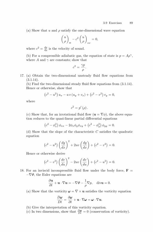
3.9 Exercises 89
(a) Show that u and ρ satisfy the one-dimensional wave equation(uρ
)tt
− c2(
uρ
)xx
= 0,
where c2 = dpdρ is the velocity of sound.
(b) For a compressible adiabatic gas, the equation of state is p = Aργ ,where A and γ are constants; show that
c2 =γp
ρ.
17. (a) Obtain the two-dimensional unsteady fluid flow equations from(3.1.14).(b) Find the two-dimensional steady fluid flow equations from (3.1.14).Hence or otherwise, show that(
c2 − u2)ux − u v (uy + vx) +(c2 − v2) vy = 0,
where
c2 = p′ (ρ) .
(c) Show that, for an irrotational fluid flow (u = ∇φ), the above equa-tion reduces to the quasi-linear partial differential equations(
c2 − φ2x
)φxx − 2φxφyφxy +
(c2 − φ2
y
)φyy = 0.
(d) Show that the slope of the characteristic C satisfies the quadraticequation (
c2 − u2)(dy
dx
)2
+ 2uv
(dy
dx
)+
(c2 − v2) = 0.
Hence or otherwise derive(c2 − v2)(
dv
du
)2
− 2uv
(dv
du
)+
(c2 − u2) = 0.
18. For an inviscid incompressible fluid flow under the body force, F =−∇Φ, the Euler equations are
∂u∂t
+ u · ∇u = −∇Φ − 1ρ∇p, divu = 0.
(a) Show that the vorticity ωωω = ∇ × u satisfies the vorticity equation
Dωωω
Dt=
∂ωωω
∂t+ u · ∇ωωω = ωωω · ∇u.
(b) Give the interpretation of this vorticity equation.(c) In two dimensions, show that Dωωω
Dt = 0 (conservation of vorticity).

90 3 Mathematical Models
19. The evolution of the probability distribution function u (x, t) in nonequi-librium statistical mechanics is described by the Fokker–Planck equa-tion (See Reif (1965))
∂u
∂t=
∂
∂x
(∂u
∂t+ x
)u.
(a) Use the change of variables
ξ = x et and v = u e−t
to show that the Fokker–Planck equation assumes the form withu (x, t) = et v (ξ, τ)
vt = e2t vξξ.
(b) Make a suitable change of variable t to τ (t), and transform theabove equation into the standard diffusion equation
vt = vξξ.
20. The electric field E (x) and the electromagnetic field H (x) in freespace (a vacuum) satisfy the Maxwell equations Et = c curl H, Ht =−c curl H, divE = 0 = divH, where c is the constant speed of light in avacuum. Show that both E and H the three-dimensional wave equations
Ett = c2∇2E and Htt = c2∇2H,
where x = (x, y, z) and ∇2 is the three-dimensional Laplacian.
21. Consider longitudinal vibrations of a free elastic rod with a variablecross section A (x) with x measured along the axis of the rod fromthe origin. Assuming that the material of the rod satisfies Hooke’s law,show that the displacement function u (x, t) satisfies the generalizedwave equation
utt = c2uxx +c2
A (x)
(dA
dx
)ux,
where c2 = (λ/ρ), λ is a constant that describes the elastic nature of thematerial, and ρ is the line density of the rod. When A (x) is constant,the above equation reduces to one-dimensional wave equation.

4
Classification of Second-Order LinearEquations
“When we have a good understanding of the problem, we are able to clearit of all auxiliary notions and to reduce it to simplest element.”
Rene Descartes
“The first process ... in the effectual study of sciences must be one of sim-plification and reduction of the results of previous investigations to a formin which the mind can grasp them.”
James Clerk Maxwell
4.1 Second-Order Equations in Two IndependentVariables
The general linear second-order partial differential equation in one depen-dent variable u may be written as
n∑i,j=1
Aijuxixj +n∑
i=1
Biuxi + Fu = G, (4.1.1)
in which we assume Aij = Aji and Aij , Bi, F , and G are real-valuedfunctions defined in some region of the space (x1, x2, . . . , xn).
Here we shall be concerned with second-order equations in the depen-dent variable u and the independent variables x, y. Hence equation (4.1.1)can be put in the form
Auxx + Buxy + Cuyy + Dux + Euy + Fu = G, (4.1.2)
where the coefficients are functions of x and y and do not vanish simulta-neously. We shall assume that the function u and the coefficients are twicecontinuously differentiable in some domain in R
2.

92 4 Classification of Second-Order Linear Equations
The classification of partial differential equations is suggested by theclassification of the quadratic equation of conic sections in analytic geom-etry. The equation
Ax2 + Bxy + Cy2 + Dx + Ey + F = 0,
represents hyperbola, parabola, or ellipse accordingly as B2 − 4AC is pos-itive, zero, or negative.
The classification of second-order equations is based upon the possibilityof reducing equation (4.1.2) by coordinate transformation to canonical orstandard form at a point. An equation is said to be hyperbolic, parabolic,or elliptic at a point (x0, y0) accordingly as
B2 (x0, y0) − 4A (x0, y0) C (x0, y0) (4.1.3)
is positive, zero, or negative. If this is true at all points, then the equationis said to be hyperbolic, parabolic, or elliptic in a domain. In the case oftwo independent variables, a transformation can always be found to reducethe given equation to canonical form in a given domain. However, in thecase of several independent variables, it is not, in general, possible to findsuch a transformation.
To transform equation (4.1.2) to a canonical form we make a change ofindependent variables. Let the new variables be
ξ = ξ (x, y) , η = η (x, y) . (4.1.4)
Assuming that ξ and η are twice continuously differentiable and that theJacobian
J =
∣∣∣∣∣∣ξx ξy
ηx ηy
∣∣∣∣∣∣ , (4.1.5)
is nonzero in the region under consideration, then x and y can be deter-mined uniquely from the system (4.1.4). Let x and y be twice continuouslydifferentiable functions of ξ and η. Then we have
ux = uξξx + uηηx, uy = uξξy + uηηy,
uxx = uξξξ2x + 2uξηξxηx + uηηη2
x + uξξxx + uηηxx, (4.1.6)uxy = uξξξxξy + uξη (ξxηy + ξyηx) + uηηηxηy + uξξxy + uηηxy,
uyy = uξξξ2y + 2uξηξyηy + uηηη2
y + uξξyy + uηηyy.
Substituting these values in equation (4.1.2) we obtain
A∗uξξ + B∗uξη + C∗uηη + D∗uξ + E∗uη + F ∗u = G∗, (4.1.7)
where

4.2 Canonical Forms 93
A∗ = Aξ2x + Bξxξy + Cξ2
y ,
B∗ = 2Aξxηx + B (ξxηy + ξyηx) + 2Cξyηy,
C∗ = Aη2x + Bηxηy + Cη2
y,
D∗ = Aξxx + Bξxy + Cξyy + Dξx + Eξy, (4.1.8)E∗ = Aηxx + Bηxy + Cηyy + Dηx + Eηy,
F ∗ = F, G∗ = G.
The resulting equation (4.1.7) is in the same form as the original equation(4.1.2) under the general transformation (4.1.4). The nature of the equationremains invariant under such a transformation if the Jacobian does notvanish. This can be seen from the fact that the sign of the discriminantdoes not alter under the transformation, that is,
B∗2 − 4A∗C∗ = J2 (B2 − 4AC
), (4.1.9)
which can be easily verified. It should be noted here that the equation canbe of a different type at different points of the domain, but for our purposewe shall assume that the equation under consideration is of the single typein a given domain.
The classification of equation (4.1.2) depends on the coefficients A (x, y),B (x, y), and C (x, y) at a given point (x, y). We shall, therefore, rewriteequation (4.1.2) as
Auxx + Buxy + Cuyy = H (x, y, u, ux, uy) , (4.1.10)
and equation (4.1.7) as
A∗uξξ + B∗uξη + C∗uηη = H∗ (ξ, η, u, uξ, uη) . (4.1.11)
4.2 Canonical Forms
In this section we shall consider the problem of reducing equation (4.1.10)to canonical form.
We suppose first that none of A, B, C, is zero. Let ξ and η be newvariables such that the coefficients A∗ and C∗ in equation (4.1.11) vanish.Thus, from (4.1.8), we have
A∗ = Aξ2x + Bξxξy + Cξ2
y = 0,
C∗ = Aη2x + Bηxηy + Cη2
y = 0.
These two equations are of the same type and hence we may write them inthe form
Aζ2x + Bζxζy + Cζ2
y = 0, (4.2.1)

94 4 Classification of Second-Order Linear Equations
in which ζ stand for either of the functions ξ or η. Dividing through by ζ2y ,
equation (4.2.1) becomes
A
(ζx
ζy
)2
+ B
(ζx
ζy
)+ C = 0. (4.2.2)
Along the curve ζ = constant, we have
dζ = ζxdx + ζydy = 0.
Thus,
dy
dx= −ζx
ζy, (4.2.3)
and therefore, equation (4.2.2) may be written in the form
A
(dy
dx
)2
− B
(dy
dx
)+ C = 0, (4.2.4)
the roots of which are
dy
dx=
(B +
√B2 − 4AC
)/2A, (4.2.5)
dy
dx=
(B −
√B2 − 4AC
)/2A. (4.2.6)
These equations, which are known as the characteristic equations, are or-dinary differential equations for families of curves in the xy-plane alongwhich ξ = constant and η = constant. The integrals of equations (4.2.5)and (4.2.6) are called the characteristic curves. Since the equations arefirst-order ordinary differential equations, the solutions may be written as
φ1 (x, y) = c1, c1 = constant,φ2 (x, y) = c2, c2 = constant.
Hence the transformations
ξ = φ1 (x, y) , η = φ2 (x, y) ,
will transform equation (4.1.10) to a canonical form.
(A) Hyperbolic TypeIf B2 − 4AC > 0, then integration of equations (4.2.5) and (4.2.6) yield
two real and distinct families of characteristics. Equation (4.1.11) reducesto
uξη = H1, (4.2.7)

4.2 Canonical Forms 95
where H1 = H∗/B∗. It can be easily shown that B∗ = 0. This form is calledthe first canonical form of the hyperbolic equation.
Now if new independent variables
α = ξ + η, β = ξ − η, (4.2.8)
are introduced, then equation (4.2.7) is transformed into
uαα − uββ = H2 (α, β, u, uα, uβ) . (4.2.9)
This form is called the second canonical form of the hyperbolic equation.
(B) Parabolic TypeIn this case, we have B2 − 4AC = 0, and equations (4.2.5) and (4.2.6)
coincide. Thus, there exists one real family of characteristics, and we obtainonly a single integral ξ = constant (or η = constant).
Since B2 = 4AC and A∗ = 0, we find that
A∗ = Aξ2x + Bξxξy + Cξ2
y =(√
A ξx +√
C ξy
)2= 0.
From this it follows that
A∗ = 2Aξxηx + B (ξxηy + ξyηx) + 2Cξyηy
= 2(√
A ξx +√
C ξy
)(√A ηx +
√C ηy
)= 0,
for arbitrary values of η (x, y) which is functionally independent of ξ (x, y);for instance, if η = y, the Jacobian does not vanish in the domain of parabol-icity.
Division of equation (4.1.11) by C∗ yields
uηη = H3 (ξ, η, u, uξ, uη) , C∗ = 0. (4.2.10)
This is called the canonical form of the parabolic equation.Equation (4.1.11) may also assume the form
uξξ = H∗3 (ξ, η, u, uξ, uη) , (4.2.11)
if we choose η = constant as the integral of equation (4.2.5).
(C) Elliptic TypeFor an equation of elliptic type, we have B2 − 4AC < 0. Consequently,
the quadratic equation (4.2.4) has no real solutions, but it has two complexconjugate solutions which are continuous complex-valued functions of thereal variables x and y. Thus, in this case, there are no real characteristiccurves. However, if the coefficients A, B, and C are analytic functions ofx and y, then one can consider equation (4.2.4) for complex x and y. Afunction of two real variables x and y is said to be analytic in a certaindomain if in some neighborhood of every point (x0, y0) of this domain, the

96 4 Classification of Second-Order Linear Equations
function can be represented as a Taylor series in the variables (x − x0) and(y − y0).
Since ξ and η are complex, we introduce new real variables
α =12
(ξ + η) , β =12i
(ξ − η) , (4.2.12)
so that
ξ = α + iβ, η = α − iβ. (4.2.13)
First, we transform equations (4.1.10). We then have
A∗∗ (α, β) uαα + B∗∗ (α, β) uαβ + C∗∗ (α, β) uββ = H4 (α, β, u, uα, uβ) ,
(4.2.14)
in which the coefficients assume the same form as the coefficients in equation(4.1.11). With the use of (4.2.13), the equations A∗ = C∗ = 0 become(
Aα2x + Bαxαy + Cα2
y
) − (Aβ2
x + Bβxβy + Cβ2y
)+i [2Aαxβx + B (αxβy + αyβx) + 2Cαyβy] = 0,
(Aα2
x + Bαxαy + Cα2y
) − (Aβ2
x + Bβxβy + Cβ2y
)−i [2Aαxβx + B (αxβy + αyβx) + 2Cαyβy] = 0,
or,
(A∗∗ − C∗∗) + iB∗∗ = 0, (A∗∗ − C∗∗) − iB∗∗ = 0.
These equations are satisfied if and only if
A∗∗ = C∗∗ and B∗∗ = 0.
Hence, equation (4.2.14) transforms into the form
A∗∗uαα + A∗∗uββ = H4 (α, β, u, uα, uβ) .
Dividing through by A∗∗, we obtain
uαα + uββ = H5 (α, β, u, uα, uβ) , (4.2.15)
where H5 = (H4/A∗∗). This is called the canonical form of the elliptic
equation.We close this discussion of canonical forms by adding an important
comment. From mathematical and physical points of view, characteristicsor characteristic coordinates play a very important physical role in hyper-bolic equations. However, they do not play a particularly physical role inparabolic and elliptic equations, but their role is somewhat mathematical

4.2 Canonical Forms 97
in solving these equations. In general, first-order partial differential equa-tions such as advection-reaction equations are regarded as hyperbolic be-cause they describe propagation of waves like the wave equation. On theother hand, second-order linear partial differential equations with constantcoefficients are sometimes classified by the associated dispersion relationω = ω (κκκ) as defined in Section 13.3. In one-dimensional case, ω = ω (k).If ω (k) is real and ω′′ (k) = 0, the equation is called dispersive. The worddispersive simply means that the phase velocity cp = (ω/k) of a plane wavesolution, u (x, t) = A exp [i (kx − ωt)] depends on the wavenumber k. Thismeans that waves of different wavelength propagate with different phase ve-locities and hence, disperse in the medium. If ω = ω (k) = σ (k) + iµ (k) iscomplex, the associated partial differential equation is called diffusive. Froma physical point of view, such a classification of equations is particularlyuseful. Both dispersive and diffusive equations are physically important,and such equations will be discussed in Chapter 13.
Example 4.2.1. Consider the equation
y2uxx − x2uyy = 0.
Here
A = y2, B = 0, C = −x2.
Thus,
B2 − 4AC = 4x2y2 > 0.
The equation is hyperbolic everywhere except on the coordinate axes x = 0and y = 0. From the characteristic equations (4.2.5) and (4.2.6), we have
dy
dx=
x
y,
dy
dx= −x
y.
After integration of these equations, we obtain
12y2 − 1
2x2 = c1,
12y2 +
12x2 = c2.
The first of these curves is a family of hyperbolas
12y2 − 1
2x2 = c1,
and the second is a family of circles
12y2 +
12x2 = c2.
To transform the given equation to canonical form, we consider

98 4 Classification of Second-Order Linear Equations
ξ =12y2 − 1
2x2, η =
12y2 +
12x2.
From the relations (4.1.6), we have
ux = uξξx + uηηx = −xuξ + xuη,
uy = uξξy + uηηy = yuξ + yuη,
uxx = uξξξ2x + 2uξηξxηx + uηηη2
x + uξξxx + uηηxx
= x2uξξ − 2x2uξη + x2uηη − uξ + uη.
uyy = uξξξ2y + 2uξηξyηy + uηηη2
y + uξξyy + uηηyy
= y2uξξ + 2y2uξη + y2uηη + uξ + uη.
Thus, the given equation assumes the canonical form
uξη =η
2 (ξ2 − η2)uξ − ξ
2 (ξ2 − η2)uη.
Example 4.2.2. Consider the partial differential equation
x2uxx + 2xy uxy + y2uyy = 0.
In this case, the discriminant is
B2 − 4AC = 4x2y2 − 4x2y2 = 0.
The equation is therefore parabolic everywhere. The characteristic equationis
dy
dx=
y
x,
and hence, the characteristics are
y
x= c,
which is the equation of a family of straight lines.Consider the transformation
ξ =y
x, η = y,
where η is chosen arbitrarily. The given equation is then reduced to thecanonical form
y2uηη = 0.
Thus,
uηη = 0 for y = 0.
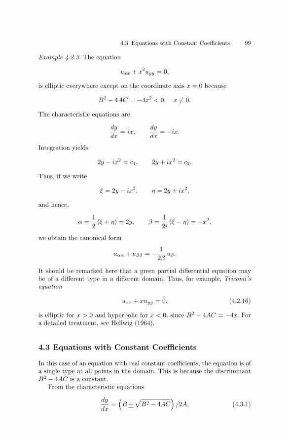
4.3 Equations with Constant Coefficients 99
Example 4.2.3. The equation
uxx + x2uyy = 0,
is elliptic everywhere except on the coordinate axis x = 0 because
B2 − 4AC = −4x2 < 0, x = 0.
The characteristic equations are
dy
dx= ix,
dy
dx= −ix.
Integration yields
2y − ix2 = c1, 2y + ix2 = c2.
Thus, if we write
ξ = 2y − ix2, η = 2y + ix2,
and hence,
α =12
(ξ + η) = 2y, β =12i
(ξ − η) = −x2,
we obtain the canonical form
uαα + uββ = − 12β
uβ .
It should be remarked here that a given partial differential equation maybe of a different type in a different domain. Thus, for example, Tricomi’sequation
uxx + xuyy = 0, (4.2.16)
is elliptic for x > 0 and hyperbolic for x < 0, since B2 − 4AC = −4x. Fora detailed treatment, see Hellwig (1964).
4.3 Equations with Constant Coefficients
In this case of an equation with real constant coefficients, the equation is ofa single type at all points in the domain. This is because the discriminantB2 − 4AC is a constant.
From the characteristic equations
dy
dx=
(B +
√B2 − 4AC
)/2A, (4.3.1)

100 4 Classification of Second-Order Linear Equations
we can see that the characteristics
y =
(B +
√B2 − 4AC
2A
)x + c1, y =
(B − √
B2 − 4AC
2A
)x + c2, (4.3.2)
are two families of straight lines. Consequently, the characteristic coordi-nates take the form
ξ = y − λ1x, η = y − λ2x, (4.3.3)
where
λ1,2 =B+
√B2 − 4AC
2A. (4.3.4)
The linear second-order partial differential equation with constant coeffi-cients may be written in the general form as
Auxx + Buxy + Cuyy + Dux + Euy + Fu = G (x, y) . (4.3.5)
In particular, the equation
Auxx + Buyy + Cuyy = 0, (4.3.6)
is called the Euler equation.
(A) Hyperbolic TypeIf B2 − 4AC > 0, the equation is of hyperbolic type, in which case the
characteristics form two distinct families.Using (4.3.3), equation (4.3.5) becomes
uξη = D1uξ + E1uη + F1u + G1 (ξ, η) , (4.3.7)
where D1, E1, and F1 are constants. Here, since the coefficients are con-stants, the lower order terms are expressed explicitly.
When A = 0, equation (4.3.1) does not hold. In this case, the charac-teristic equation may be put in the form
−B (dx/dy) + C (dx/dy)2 = 0,
which may again be rewritten as
dx/dy = 0, and − B + C (dx/dy) = 0.
Integration gives
x = c1, x = (B/C) y + c2,
where c1 and c2 are integration constants. Thus, the characteristic coordi-nates are

4.3 Equations with Constant Coefficients 101
ξ = x, η = x − (B/C) y. (4.3.8)
Under this transformation, equation (4.3.5) reduces to the canonical form
uξη = D∗1uξ + E∗
1uη + F ∗1 u + G∗
1 (ξ, η) , (4.3.9)
where D∗1 , E∗
1 , and F ∗1 are constants.
The canonical form of the Euler equation (4.3.6) is
uξη = 0. (4.3.10)
Integrating this equation gives the general solution
u = φ (ξ) + ψ (η) = φ (y − λ1, x) + ψ (y − λ2, x) , (4.3.11)
where φ and ψ are arbitrary functions, and λ1 and λ2 are given by (4.3.3).
(B) Parabolic TypeWhen B2 − 4AC = 0, the equation is of parabolic type, in which case
only one real family of characteristics exists. From equation (4.3.4), we findthat
λ1 = λ2 = (B/2A) ,
so that the single family of characteristics is given by
y = (B/2A) x + c1,
where c1 is an integration constant. Thus, we have
ξ = y − (B/2A) x, η = hy + kx, (4.3.12)
where η is chosen arbitrarily such that the Jacobian of the transformationis not zero, and h and k are constants.
With the proper choice of the constants h and k in the transformation(4.3.12), equation (4.3.5) reduces to
uηη = D2uξ + E2uη + F2u + G2 (ξ, η) , (4.3.13)
where D2, E2, and F2 are constants.If B = 0, we can see at once from the relation
B2 − 4AC = 0,
that C or A vanishes. The given equation is then already in the canonicalform. Similarly, in the other cases when A or C vanishes, B vanishes. Thegiven equation is is then also in canonical form.
The canonical form of the Euler equation (4.3.6) is
uηη = 0. (4.3.14)

102 4 Classification of Second-Order Linear Equations
Integrating twice gives the general solution
u = φ (ξ) + η ψ (ξ) , (4.3.15)
where ξ and η are given by (4.3.12). Choosing h = 1, k = 0 and λ =(
B2A
)for simplicity, the general solution of the Euler equation in the paraboliccase is
u = φ (y − λx) + y ψ (y − λx) . (4.3.16)
(C) Elliptic TypeWhen B2 − 4AC < 0, the equation is of elliptic type. In this case, the
characteristics are complex conjugates.The characteristic equations yield
y = λ1x + c1, y = λ2x + c2, (4.3.17)
where λ1 and λ2 are complex numbers. Accordingly, c1 and c2 are allowedto take on complex values. Thus,
ξ = y − (a + ib) x, η = y − (a − ib) x, (4.3.18)
where λ1,2 = a + ib in which a and b are real constants, and
a =B
2A, and b =
12A
√4AC − B2 .
Introduce the new variables
α =12
(ξ + η) = y − ax, β =12i
(ξ − η) = −bx. (4.3.19)
Application of this transformation readily reduces equation (4.3.5) to thecanonical form
uαα + uββ = D3uα + E3uβ + F3u + G3 (α, β) , (4.3.20)
where D3, E3, F3 are constants.We note that B2 − AC < 0, so neither A nor C is zero.In this elliptic case, the Euler equation (4.3.6) gives the complex char-
acteristics (4.3.18) which are
ξ = (y − ax) − ibx, η = (y − ax) + ibx = ξ. (4.3.21)
Consequently, the Euler equation becomes
uξξ = 0, (4.3.22)
with the general solution
u = φ (ξ) + ψ(ξ). (4.3.23)
The appearance of complex arguments in the general solution (4.3.23) is ageneral feature of elliptic equations.

4.3 Equations with Constant Coefficients 103
Example 4.3.1. Consider the equation
4 uxx + 5 uxy + uyy + ux + uy = 2.
Since A = 4, B = 5, C = 1, and B2 − 4AC = 9 > 0, the equation ishyperbolic. Thus, the characteristic equations take the form
dy
dx= 1,
dy
dx=
14,
and hence, the characteristics are
y = x + c1, y = (x/4) + c2.
The linear transformation
ξ = y − x, η = y − (x/4) ,
therefore reduces the given equation to the canonical form
uξη =13
uη − 89.
This is the first canonical form.The second canonical form may be obtained by the transformation
α = ξ + η, β = ξ − η,
in the form
uαα − uββ =13
uα − 13
uβ − 89.
Example 4.3.2. The equation
uxx − 4 uxy + 4 uyy = ey,
is parabolic since A = 1, B = −4, C = 4, and B2 − 4AC = 0. Thus, wehave from equation (4.3.12)
ξ = y + 2x, η = y,
in which η is chosen arbitrarily. By means of this mapping, the equationtransforms into
uηη =14
eη.
Example 4.3.3. Consider the equation
uxx + uxy + uyy + ux = 0.

104 4 Classification of Second-Order Linear Equations
Since A = 1, B = 1, C = 1, and B2 − 4AC = −3 < 0, the equation iselliptic.
We have
λ1,2 =B +
√B2 − 4AC
2A=
12
+ i
√3
2,
and hence,
ξ = y −(
12
+ i
√3
2
)x, η = y −
(12
− i
√3
2
)x.
Introducing the new variables
α =12
(ξ + η) = y − 12x, β =
12i
(ξ − η) = −√
32
x,
the given equation is then transformed into canonical form
uαα + uββ =23
uα +2√3
uβ .
Example 4.3.4. Consider the wave equation
utt − c2uxx = 0, c is constant.
Since A = −c2, B = 0, C = 1, and B2 − 4AC = 4c2 > 0, the waveequation is hyperbolic everywhere. According to (4.2.4), the equation ofcharacteristics is
−c2(
dt
dx
)2
+ 1 = 0,
or
dx2 − c2dt2 = 0.
Therefore,
x + ct = ξ = constant, x − ct = η = constant.
Thus, the characteristics are straight lines, which are shown in Figure 4.3.1.The characteristics form a natural set of coordinates for the hyperbolicequation.
In terms of new coordinates ξ and η defined above, we obtain
uxx = uξξ + 2uξη + uηη,
utt = c2 (uξξ − 2uξη + uηη) ,
so that the wave equation becomes

4.3 Equations with Constant Coefficients 105
Figure 4.3.1 Characteristics for the wave equation.
−4c2uξη = 0.
Since c = 0, we have
uξη = 0.
Integrating with respect to ξ, we obtain
uη = ψ1 (η) .
where ψ1 is the arbitrary function of η. Integrating with respect to η, weobtain
u (ξ, η) =∫
ψ1 (η) dη + φ (ξ) .
If we set ψ (η) =∫
ψ1 (η) dη, the general solution becomes
u (ξ, η) = φ (ξ) + ψ (η) ,
which is, in terms of the original variables x and t,
u (x, t) = φ (x + ct) + ψ (x − ct) ,
provided φ and ψ are arbitrary but twice differentiable functions.

106 4 Classification of Second-Order Linear Equations
Note that φ is constant on “wavefronts” x = −ct + ξ that travel towarddecreasing x as t increases, whereas ψ is constant on wavefronts x = ct + ηthat travel toward increasing x as t increases. Thus, any general solutioncan be expressed as the sum of two waves, one traveling to the right withconstant velocity c and the other traveling to the left with the same velocityc.
Example 4.3.5. Find the characteristic equations and characteristics, andthen reduce the equations
uxx +(sech4x
)uyy = 0, (4.3.24ab)
to the canonical forms.In equation (4.3.24a), A = 1, B = 0 and C = −sech4x. Hence,
B2 − 4AC = 4 sech4x > 0.
Hence, the equation is hyperbolic. The characteristic equations are
dy
dx=
B +√
B2 − 4AC
2A= + sech2x.
Integration gives
y + tanhx = constant.
Hence,
ξ = y + tanhx, η = y − tanhx.
Using these characteristic coordinates, the given equation can be trans-formed into the canonical form
uξη =(η − ξ)[
4 − (ξ − η)2] (uξ − uη) . (4.3.25)
In equation (4.3.24b), A = 1, B = 0 and C = sech4x. Hence,
B2 − 4AC = + i sech2x.
Integrating gives
y + i tanhx = constant.
Thus,
ξ = y + i tanhx, η = y − i tanhx.
The new real variables α and β are

4.4 General Solutions 107
α =12
(ξ + η) = y, β =12i
(ξ − η) = tanhx.
In terms of these new variables, equation (4.3.24b) can be transformed intothe canonical form
uαα + uββ =2β
1 − β2 uβ , |β| < 1. (4.3.26)
Example 4.3.6. Consider the equation
uxx + (2 cosecy) uxy +(cosec2y
)uyy = 0. (4.3.27)
In this case, A = 1, B = 2 cosecy and C = cosec2y. Hence, B2 − 4AC = 0,and
dy
dx=
B
2A= cosec y.
The characteristic curves are therefore given by
ξ = x + cos y and η = y.
Using these variables, the canonical form of (4.3.27) is
uηη =(sin2 η cos η
)uξ. (4.3.28)
4.4 General Solutions
In general, it is not so simple to determine the general solution of a givenequation. Sometimes further simplification of the canonical form of an equa-tion may yield the general solution. If the canonical form of the equationis simple, then the general solution can be immediately ascertained.
Example 4.4.1. Find the general solution of
x2uxx + 2xy uxy + y2uyy = 0.
In Example 4.2.2, using the transformation ξ = y/x, η = y, this equationwas reduced to the canonical form
uηη = 0, for y = 0.
Integrating twice with respect to η, we obtain
u (ξ, η) = ηf (ξ) + g (ξ) ,
where f (ξ) and g (ξ) are arbitrary functions. In terms of the independentvariables x and y, we have
u (x, y) = y f(y
x
)+ g
(y
x
).

108 4 Classification of Second-Order Linear Equations
Example 4.4.2. Determine the general solution of
4 uxx + 5 uxy + uyy + ux + uy = 2.
Using the transformation ξ = y − x, η = y − (x/4), the canonical form ofthis equation is (see Example 4.3.1)
uξη =13
uη − 89.
By means of the substitution v = uη, the preceding equation reduces to
vξ =13
v − 89.
This can be easily integrated by separating the variables. Integrating withrespect to ξ, we have
v =83
+13
e(ξ/3)F (η) .
Integrating with respect to η, we obtain
u (ξ, η) =83
η +13g (η) eξ/3 + f (ξ) ,
where f (ξ) and g (η) are arbitrary functions. The general solution of thegiven equation becomes
u (x, y) =83
(y − 1
4
)+
13
g(y − x
4
)e
13 (y−x) + f (y − x) .
Example 4.4.3. Obtain the general solution of
3 uxx + 10 uxy + 3 uyy = 0.
Since B2 − 4AC = 64 > 0, the equation is hyperbolic. Thus, from equation(4.3.2), the characteristics are
y = 3x + c1, y =13x + c2.
Using the transformations
ξ = y − 3x, η = y − 13x,
the given equation can be reduced to the form(643
)uξη = 0.

4.4 General Solutions 109
Hence, we obtain
uξη = 0.
Integration yields
u (ξ, η) = f (ξ) + g (η) .
In terms of the original variables, the general solution is
u (x, y) = f (y − 3x) + g(y − x
3
).
Example 4.4.4. Find the general solution of the following equations
y uxx + 3 y uxy + 3 ux = 0, y = 0, (4.4.1)uxx + 2 uxy + uyy = 0, (4.4.2)
uxx + 2 uxy + 5 uyy + ux = 0. (4.4.3)
In equation (4.4.1), A = y, B = 3y, C = 0, D = 3, E = F = G = 0.Hence B2 − 4AC = 9y2 > 0 and the equation is hyperbolic for all points(x, y) with y = 0. Consequently, the characteristic equations are
dy
dx=
B +√
B2 − 4AC
2A=
3y + 3y
2y= 3, 0.
Integrating gives
y = c1 and y = 3x + c2.
The characteristic curves are
ξ = y and η = y − 3x.
In terms of these variables, the canonical form of (4.4.1) is
ξ uξη + uη = 0.
Writing v = uη and using the integrating factor gives
v = uη =1ξ
C (η) ,
where C (η) is an arbitrary function.Integrating again with respect to η gives
u (ξ, η) =1ξ
∫C (η) dη + g (ξ) =
1ξf (η) + g (ξ) ,
where f and g are arbitrary functions. Finally, in terms of the originalvariables, the general solution is

110 4 Classification of Second-Order Linear Equations
u (x, y) =1y
f (y − 3x) + g (y) . (4.4.4)
Equation (4.4.2) has coefficients A = 1, B = 2, C = 1, D = E = F =G = 0. Hence, B2 − 4AC = 0, the equation is parabolic. The characteristicequation is
dy
dx= 1,
and the characteristics are
ξ = y − x = c1 and η = y.
Using these variables, equation (4.4.2) takes the canonical form
uηη = 0.
Integrating twice gives the general solution
u (ξ, η) = η f (ξ) + g (ξ) ,
where f and g are arbitrary functions.In terms of x and y, this solution becomes
u (x, y) = y f (y − x) + g (y − x) . (4.4.5)
The coefficients of equation (4.4.3) are A = 1, B = 2, C = 5, E = 1,F = G = 0 and hence B2 − 4AC = −16 < 0, equation (4.4.3) is elliptic.The characteristic equations are
dy
dx= (1 +2i) .
The characteristics are
y = (1 − 2i) x + c1, y = (1 + 2i) x + c2,
and hence,
ξ = y − (1 − 2i) x, η = y − (1 + 2i) x,
and new real variables α and β are
α =12
(ξ + η) = y − x, η =12i
(ξ − η) = 2x.
The canonical form is given by
(uαα + uββ) =14
(uα − 2 uβ) . (4.4.6)
It is not easy to find a general solution of (4.4.6).

4.5 Summary and Further Simplification 111
Example 4.4.5. Use u = f (ξ), ξ = x√4κt
to solve the parabolic system
ut = κuxx, −∞ < x < ∞, t > 0, (4.4.7)u (x, 0) = 0, x < 0; u (x, 0) = u0, x > 0, (4.4.8)
where κ and u0 are constant.We use the given transformations to obtain
ut = f ′ (ξ) ξt = −12
x√4κt3
f ′ (ξ) ,
uxx =∂
∂x(ux) =
∂
∂x(f ′ (ξ) · ξx) =
14κt
f ′′ (ξ) .
Consequently, equation (4.4.7) becomes
f ′′ (ξ) + 2 ξf ′ (ξ) = 0.
The solution of this equation is
f ′ (ξ) = A exp(−ξ2) ,
where A is a constant of integration. Integrating again gives
f (ξ) = A
∫ ξ
0e−α2
dα + B,
where B is an integrating constant.Using the given conditions yields
0 = A
∫ −∞
0e−α2
dα + B, u0 = A
∫ ∞
0e−α2
dα + B,
which give
A =u0√π
and B =12
u0.
Thus, the final solution is
u (x, t) = u0
[1√π
∫ x√4κt
0e−α2
dα +12
].
4.5 Summary and Further Simplification
We summarize the classification of linear second-order partial differentialequations with constant coefficients in two independent variables.

112 4 Classification of Second-Order Linear Equations
hyperbolic: urs = a1ur + a2us + a3u + f1, (4.5.1)urr − uss = a∗
1ur + a∗2us + a∗
3u + f∗1 , (4.5.2)
parabolic: urs = b1ur + b2us + b3u + f2, (4.5.3)elliptic: urr + uss = c1ur + c2us + c3u + f3, (4.5.4)
where r and s represent the new independent variables in the linear trans-formations
r = r (x, y) , s = s (x, y) , (4.5.5)
and the Jacobian J = 0.To simplify equation (4.5.1) further, we introduce the new dependent
variable
v = u e−(ar+bs), (4.5.6)
where a and b are undetermined coefficients. Finding the derivatives, weobtain
ur = (vr + av) ear+bs,
us = (vs + bv) ear+bs,
urr =(vrr + 2avr + a2v
)ear+bs,
urs = (vrs + avs + bvr + abv) ear+bs,
uss =(vss + 2bvs + b2v
)ear+bs.
Substitution of these equation (4.5.1) yields
vrs + (b − a1) vr + (a − a2) vs + (ab − a1a − a2b − a3) v = f1 e−(ar+bs).
In order that the first derivatives vanish, we set
b = a1 and a = a2.
Thus, the above equation becomes
vrs = (a1a2 + a3) v + g1,
where g1 = f1 e−(a2r+a1s). In a similar manner, we can transform equa-tions (4.5.2)–(4.5.4). Thus, we have the following transformed equationscorresponding to equations (4.5.1)–(4.5.4).
hyperbolic: vrs = h1v + g1,
vrr − vss = h∗1v + g∗
1 , (4.5.7)parabolic: vss = h2v + g2,
elliptic: vrr + vss = h3v + g3.
In the case of partial differential equations in several independent vari-ables or in higher order, the classification is considerably more complex.For further reading, see Courant and Hilbert (1953, 1962).

4.6 Exercises 113
4.6 Exercises
1. Determine the region in which the given equation is hyperbolic, parabolic,or elliptic, and transform the equation in the respective region to canon-ical form.
(a) xuxx + uyy = x2, (b) uxx + y2uyy = y,
(c) uxx + xyuyy = 0, (d) x2uxx − 2xyuxy + y2uyy = ex,
(e) uxx + uxy − xuyy = 0, (f) exuxx + eyuyy = u,
(g) uxx − √y uxy +
(x4
)uyy + 2x ux − 3y uy + 2u = exp
(x2 − 2y
),
y ≥ 0,
(h) uxx − √y uxy + xuyy = cos
(x2 − 2y
), y ≥ 0,
(i) uxx − yuxy + xux + yuy + u = 0,
(j) sin2 x uxx + sin 2x uxy + cos2 x uyy = x,
2. Obtain the general solution of the following equations:
(i) x2uxx + 2xyuxy + y2uyy + xyux + y2uy = 0,
(ii) rutt − c2rurr − 2c2ur = 0, c = constant,
(iii) 4ux + 12uxy + 9uyy − 9u = 9,
(iv) uxx + uxy − 2uyy − 3ux − 6uy = 9 (2x − y),
(v) yux + 3y uxy + 3ux = 0, y = 0.
(vi) uxx + uyy = 0,
(vii) 4uxx + uyy = 0,
(viii) uxx − 2 uxy + uyy = 0,
(ix) 2uxx + uyy = 0,
(x) uxx + 4 uxy + 4 uyy = 0,
(xi) 3uxx + 4 uxy − 34 uyy = 0.

114 4 Classification of Second-Order Linear Equations
3. Find the characteristics and characteristic coordinates, and reduce thefollowing equations to canonical form:
(a) uxx + 2uxy + 3uyy + 4ux + 5uy + u = ex,
(b) 2uxx − 4uxy + 2uyy + 3u = 0,
(c) uxx + 5uxy + 4uyy + 7uy = sinx, (d) uxx + uyy + 2ux + 8uy + u = 0,
(e) uxy + 2uyy + 9ux + uy = 2, (f) 6uxx − uxy + u = y2,
(g) uxy + ux + uy = 3x, (h) uyy − 9ux + 7uy = cos y,
(i) x2uxx − y2uyy − ux = 1 + 2y2, (j) uxx + yuyy + 12uy + 4yux = 0,
(k) x2y2uxx + 2xyuxy + uyy = 0, (l) uxx + yuyy = 0.
4. Determine the general solutions of the following equations:
(i) uxx − 1c2 uyy = 0, c = constant, (ii) uxx + uyy = 0,
(iii) uxxxx + 2uxxyy + uyyyy = 0, (iv) uxx − 3uxy + 2uyy = 0,
(v) uxx + uxy = 0, (vi) uxx + 10uxy + 9uyy = y.
5. Transform the following equations to the form vξη = cv, c = constant,
(i) uxx − uyy + 3ux − 2uy + u = 0,
(ii) 3uxx + 7uxy + 2uyy + uy + u = 0,
by introducing the new variables v = u e−(aξ+bη), where a and b areundetermined coefficients.
6. Given the parabolic equation
uxx = aut + bux + cu + f,
where the coefficients are constants, by the substitution u = v e12 bx, for
the case c = − (b2/4
), show that the given equation is reduced to the
heat equation
vxx = avt + g, g = fe−bx/2.
7. Reduce the Tricomi equation
uxx + xuyy = 0,

4.6 Exercises 115
to the canonical form
(i) uξη − [6 (ξ − η)]−1 (uξ − uη) = 0, for x < 0,
(ii) uαα + uββ + 13β = 0, x > 0.
Show that the characteristic curves for x < 0 are cubic parabolas.
8. Use the polar coordinates r and θ (x = r cos θ, y = r sin θ) to transformthe Laplace equation uxx + uyy = 0 into the polar form
∇2u = urr +1r
ur +1r2 uθθ = 0.
9. (a) Using the cylindrical polar coordinates x = r cos θ, y = r sin θ, z = z,transform the three-dimensional Laplace equation uxx + uyy + uzz = 0into the form
urr +1r
ur +1r2 uθθ + uzz = 0.
(b) Use the spherical polar coordinates (r, θ, φ) so that x = r sin φ cos θ,y = r sin φ sin θ, z = r cos φ to transform the three-dimensional Laplaceequation uxx + uyy + uzz = 0 into the form
urr +2r
ur +1
r2 sin φ(sin φ uφ)φ +
1r2 sin2 φ
uθθ = 0.
(c) Transform the diffusion equation
ut = κ (uxx + uyy) ,
into the axisymmetric form
ut = κ
(urr +
1r
ur
).
10. (a) Apply a linear transformation ξ = ax + by and η = cx + dy, totransform the Euler equation
A uxx + 2B uxy + C uyy = 0
into canonical form, where a, b, c, d, A, B and C are constants .(b) Show that the same transformation as in (a) can be used to trans-form the nonhomogeneous Euler equation
A uxx + 2B uxy + C uyy = F (x, y, u, ux, uy)
into canonical form.

116 4 Classification of Second-Order Linear Equations
11. Obtain the solution of the Cauchy problem
uxx + uyy = 0,
u (x, 0) = f (x) and uy (x, 0) = g (x) .
12. Classify each of the following equations and reduce it to canonical form:
(a) y uxx − x uyy = 0, x > 0, y > 0; (b) uxx +(sech4x
)uyy = 0,
(c) y2uxx + x2uyy = 0, (d) uxx − (sech4x
)uyy = 0,
(e) uxx + 6uxy + 9uyy + 3y uy = 0,
(f) y2uxx + 2xy uxy + 2x2uyy + xux = 0,
(g) uxx − (2 cos x) uxy +(1 + cos2 x
)uyy + u = 0,
(h) uxx + (2 cosec y) uxy +(cosec2y
)uyy = 0.
(i) uxx − 2 uxy + uyy + 3 ux − u + 1 = 0,
(j) uxx − y2uyy + ux − u + x2 = 0,
(k) uxx + y uyy − x uy + y = 0.
13. Transform the equation
uxy + y uyy + sin (x + y) = 0
into the canonical form. Use the canonical form to find the generalsolution.
14. Classify each of the following equations for u (x, t):
(a) ut = (p ux)x, (b) utt − c2uxx + αu = 0,
(c) (a ux)x + (a ut)t = 0, (d) uxt − a ut = 0,
where p (x), c (x, t), a (x, t), and α (x) are given functions that takeonly positive values in the (x, t) plane. Find the general solution of theequation in (d).

5
The Cauchy Problem and Wave Equations
“Since a general solution must be judged impossible from want of analysis,we must be content with the knowledge of some special cases, and that allthe more, since the development of various cases seems to be the only wayto bringing us at last to a more perfect knowledge.”
Leonhard Euler
“What would geometry be without Gauss, mathematical logic withoutBoole, algebra without Hamilton, analysis without Cauchy?”
George Temple
5.1 The Cauchy Problem
In the theory of ordinary differential equations, by the initial-value problemwe mean the problem of finding the solutions of a given differential equationwith the appropriate number of initial conditions prescribed at an initialpoint. For example, the second-order ordinary differential equation
d2u
dt2= f
(t, u,
du
dt
)and the initial conditions
u (t0) = α,
(du
dt
)(t0) = β,
constitute an initial-value problem.An analogous problem can be defined in the case of partial differential
equations. Here we shall state the problem involving second-order partialdifferential equations in two independent variables.

118 5 The Cauchy Problem and Wave Equations
We consider a second-order partial differential equation for the functionu in the independent variables x and y, and suppose that this equation canbe solved explicitly for uyy, and hence, can be represented in the from
uyy = F (x, y, u, ux, uy, uxx, uxy) . (5.1.1)
For some value y = y0, we prescribe the initial values of the unknownfunction and of the derivative with respect to y
u (x, y0) = f (x) , uy (x, y0) = g (x) . (5.1.2)
The problem of determining the solution of equation (5.1.1) satisfyingthe initial conditions (5.1.2) is known as the initial-value problem. For in-stance, the initial-value problem of a vibrating string is the problem offinding the solution of the wave equation
utt = c2uxx,
satisfying the initial conditions
u (x, t0) = u0 (x) , ut (x, t0) = v0 (x) ,
where u0 (x) is the initial displacement and v0 (x) is the initial velocity.In initial-value problems, the initial values usually refer to the data
assigned at y = y0. It is not essential that these values be given alongthe line y = y0; they may very well be prescribed along some curve L0 inthe xy plane. In such a context, the problem is called the Cauchy probleminstead of the initial-value problem, although the two names are actuallysynonymous.
We consider the Euler equation
Auxx + Buxy + Cuyy = F (x, y, u, ux, uy) , (5.1.3)
where A, B, C are functions of x and y. Let (x0, y0) denote points on asmooth curve L0 in the xy plane. Also let the parametric equations of thiscurve L0 be
x0 = x0 (λ) , y0 = y0 (λ) , (5.1.4)
where λ is a parameter.We suppose that two functions f (λ) and g (λ) are prescribed along
the curve L0. The Cauchy problem is now one of determining the solutionu (x, y) of equation (5.1.3) in the neighborhood of the curve L0 satisfyingthe Cauchy conditions
u = f (λ) , (5.1.5a)∂u
∂n= g (λ) , (5.1.5b)

5.1 The Cauchy Problem 119
on the curve L0 where n is the direction of the normal to L0 which liesto the left of L0 in the counterclockwise direction of increasing arc length.The function f (λ) and g (λ) are called the Cauchy data.
For every point on L0, the value of u is specified by equation (5.1.5a).Thus, the curve L0 represented by equation (5.1.4) with the condition(5.1.5a) yields a twisted curve L in (x, y, u) space whose projection onthe xy plane is the curve L0. Thus, the solution of the Cauchy problem is asurface, called an integral surface, in the (x, y, u) space passing through Land satisfying the condition (5.1.5b), which represents a tangent plane tothe integral surface along L.
If the function f (λ) is differentiable, then along the curve L0, we have
du
dλ=
∂u
∂x
dx
dλ+
∂u
∂y
dy
dλ=
df
dλ, (5.1.6)
and
∂u
∂n=
∂u
∂x
dx
dn+
∂u
∂y
dy
dn= g, (5.1.7)
but
dx
dn= −dy
dsand
dy
dn=
dx
ds. (5.1.8)
Equation (5.1.7) may be written as
∂u
∂n= −∂u
∂x
dy
ds+
∂u
∂y
dx
ds= g. (5.1.9)
Since ∣∣∣∣∣∣dxdλ
dydλ
−dyds
dxds
∣∣∣∣∣∣ =(dx)2 + (dy)2
ds dλ= 0, (5.1.10)
it is possible to find ux and uy on L0 from the system of equations (5.1.6)and (5.1.9). Since ux and uy are known on L0, we find the higher derivativesby first differentiating ux and uy with respect to λ. Thus, we have
∂2u
∂x2
dx
dλ+
∂2u
∂x ∂y
dy
dλ=
d
dλ
(∂u
∂x
), (5.1.11)
∂2u
∂x ∂y
dx
dλ+
∂2u
∂y2
dy
dλ=
d
dλ
(∂u
∂y
). (5.1.12)
From equation (5.1.3), we have
A∂2u
∂x2 + B∂2u
∂x ∂y+ C
∂2u
∂y2 = F, (5.1.13)

120 5 The Cauchy Problem and Wave Equations
where F is known since ux and uy have been found. The system of equationscan be solved for uxx, uxy, and uyy, if∣∣∣∣∣∣∣∣∣∣
dxdλ
dydλ 0
0 dxdλ
dydλ
A B C
∣∣∣∣∣∣∣∣∣∣= C
(dx
dλ
)2
− B
(dx
dλ
)(dy
dλ
)+ A
(dy
dλ
)2
= 0. (5.1.14)
The equation
A
(dy
dx
)2
− B
(dy
dx
)+ C = 0, (5.1.15)
is called the characteristic equation. It is then evident that the necessarycondition for obtaining the second derivatives is that the curve L0 must notbe a characteristic curve.
If the coefficients of equation (5.1.3) and the function (5.1.5) are ana-lytic, then all the derivatives of higher orders can be computed by the aboveprocess. The solution can then be represented in the form of a Taylor series:
u (x, y) =∞∑
n=0
∞∑k=0
1k! (n − k)!
∂nu0
∂xk0 ∂yn−k
0
(x − x0)k (y − y0)
n−k, (5.1.16)
which can be shown to converge in the neighborhood of the curve L0. Thus,we may state the famous Cauchy–Kowalewskaya theorem.
5.2 The Cauchy–Kowalewskaya Theorem
Let the partial differential equation be given in the form
uyy = F (y, x1, x2, . . . , xn, u, uy, ux1 , ux2 . . . , uxn ,
ux1y, ux2y, . . . , uxny, ux1x1 , ux2x2 , . . . , uxnxn) , (5.2.1)
and let the initial conditions
u = f (x1, x2, . . . , xn) , (5.2.2)uy = g (x1, x2, . . . , xn) , (5.2.3)
be given on the noncharacteristic manifold y = y0.If the function F is analytic in some neighborhood of the point(
y0, x01, x
02, . . . , x
0n, u0, u0
y, . . .)
and if the functions f and g are analytic insome neighborhood of the point
(x0
1, x02, . . . , x
0n
), then the Cauchy prob-
lem has a unique analytic solution in some neighborhood of the point(y0, x0
1, x02, . . . , x
0n
).
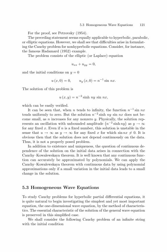
5.3 Homogeneous Wave Equations 121
For the proof, see Petrovsky (1954).The preceding statement seems equally applicable to hyperbolic, parabolic,
or elliptic equations. However, we shall see that difficulties arise in formulat-ing the Cauchy problem for nonhyperbolic equations. Consider, for instance,the famous Hadamard (1952) example.
The problem consists of the elliptic (or Laplace) equation
uxx + uyy = 0,
and the initial conditions on y = 0
u (x, 0) = 0, uy (x, 0) = n−1 sin nx.
The solution of this problem is
u (x, y) = n−2 sinh ny sin nx,
which can be easily verified.It can be seen that, when n tends to infinity, the function n−1 sin nx
tends uniformly to zero. But the solution n−2 sinh ny sin nx does not be-come small, as n increases for any nonzero y. Physically, the solution rep-resents an oscillation with unbounded amplitude
(n−2 sinhny
)as y → ∞
for any fixed x. Even if n is a fixed number, this solution is unstable in thesense that u → ∞ as y → ∞ for any fixed x for which sinnx = 0. It isobvious then that the solution does not depend continuously on the data.Thus, it is not a properly posed problem.
In addition to existence and uniqueness, the question of continuous de-pendence of the solution on the initial data arises in connection with theCauchy–Kowalewskaya theorem. It is well known that any continuous func-tion can accurately be approximated by polynomials. We can apply theCauchy–Kowalewskaya theorem with continuous data by using polynomialapproximations only if a small variation in the initial data leads to a smallchange in the solution.
5.3 Homogeneous Wave Equations
To study Cauchy problems for hyperbolic partial differential equations, itis quite natural to begin investigating the simplest and yet most importantequation, the one-dimensional wave equation, by the method of characteris-tics. The essential characteristic of the solution of the general wave equationis preserved in this simplified case.
We shall consider the following Cauchy problem of an infinite stringwith the initial condition

122 5 The Cauchy Problem and Wave Equations
utt − c2uxx = 0, x ∈ R, t > 0, (5.3.1)u (x, 0) = f (x) , x ∈ R, (5.3.2)
ut (x, 0) = g (x) , x ∈ R. (5.3.3)
By the method of characteristics described in Chapter 4, the characteristicequation according to equation (4.2.4) is
dx2 − c2dt2 = 0,
which reduces to
dx + c dt = 0, dx − c dt = 0.
The integrals are the straight lines
x + ct = c1, x − ct = c2.
Introducing the characteristic coordinates
ξ = x + ct, η = x − ct,
we obtain
uxx = uξξ + 2 uξη + uηη, utt = c2 (uξξ − 2 uξη + uηη) .
Substitution of these in equation (5.3.1) yields
−4c2uξη = 0.
Since c = 0, we have
uξη = 0.
Integrating with respect to ξ, we obtain
uη = ψ∗ (η) ,
where ψ∗ (η) is an arbitrary function of η. Integrating again with respectto η, we obtain
u (ξ, η) =∫
ψ∗ (η) dη + φ (ξ) .
If we set ψ (η) =∫
ψ∗ (η) dη, we have
u (ξ, η) = φ (ξ) + ψ (η) ,
where φ and ψ are arbitrary functions. Transforming to the original vari-ables x and t, we find the general solution of the wave equation

5.3 Homogeneous Wave Equations 123
u (x, t) = φ (x + ct) + ψ (x − ct) , (5.3.4)
provided φ and ψ are twice differentiable functions.Now applying the initial conditions (5.3.2) and (5.3.3), we obtain
u (x, 0) = f (x) = φ (x) + ψ (x) , (5.3.5)ut (x, 0) = g (x) = c φ′ (x) − c ψ′ (x) . (5.3.6)
Integration of equation (5.3.6) gives
φ (x) − ψ (x) =1c
∫ x
x0
g (τ) dτ + K, (5.3.7)
where x0 and K are arbitrary constants. Solving for φ and ψ from equations(5.3.5) and (5.3.7), we obtain
φ (x) =12
f (x) +12c
∫ x
x0
g (τ) dτ +K
2,
ψ (x) =12
f (x) − 12c
∫ x
x0
g (τ) dτ − K
2.
The solution is thus given by
u (x, t) =12
[f (x + ct) + f (x − ct)] +12c
[∫ x+ct
x0
g (τ) dτ −∫ x−ct
x0
g (τ) dτ
]=
12
[f (x + ct) + f (x − ct)] +12c
∫ x+ct
x−ct
g (τ) dτ. (5.3.8)
This is called the celebrated d’Alembert solution of the Cauchy problem forthe one-dimensional wave equation.
It is easy to verify by direct substitution that u (x, t), represented by(5.3.8), is the unique solution of the wave equation (5.3.1) provided f (x)is twice continuously differentiable and g (x) is continuously differentiable.This essentially proves the existence of the d’Alembert solution. By directsubstitution, it can also be shown that the solution (5.3.8) is uniquely de-termined by the initial conditions (5.3.2) and (5.3.3). It is important to notethat the solution u (x, t) depends only on the initial values of f at pointsx − ct and x + ct and values of g between these two points. In other words,the solution does not depend at all on initial values outside this interval,x − ct ≤ x ≤ x + ct. This interval is called the domain of dependence of thevariables (x, t).
Moreover, the solution depends continuously on the initial data, thatis, the problem is well posed. In other words, a small change in eitherf or g results in a correspondingly small change in the solution u (x, t).Mathematically, this can be stated as follows:
For every ε > 0 and for each time interval 0 ≤ t ≤ t0, there exists anumber δ (ε, t0) such that

124 5 The Cauchy Problem and Wave Equations
|u (x, t) − u∗ (x, t)| < ε,
whenever
|f (x) − f∗ (x)| < δ, |g (x) − g∗ (x)| < δ.
The proof follows immediately from equation (5.3.8). We have
|u (x, t) − u∗ (x, t)| ≤ 12
|f (x + ct) − f∗ (x + ct)|
+12
|f (x − ct) − f∗ (x − ct)|
+12c
∫ x+ct
x−ct
|g (τ) − g∗ (τ)| dτ < ε,
where ε = δ (1 + t0).For any finite time interval 0 < t < t0, a small change in the initial data
only produces a small change in the solution. This shows that the problemis well posed.
Example 5.3.1. Find the solution of the initial-value problem
utt = c2uxx, x ∈ R, t > 0,
u (x, 0) = sin x, ut (x, 0) = cos x.
From (5.3.8), we have
u (x, t) =12
[sin (x + ct) + sin (x − ct)] +12c
∫ x+ct
x−ct
cos τ dτ
= sin x cos ct +12c
[sin (x + ct) − sin (x − ct)]
= sin x cos ct +1c
cos x sin ct.
It follows from the d’Alembert solution that, if an initial displacement oran initial velocity is located in a small neighborhood of some point (x0, t0),it can influence only the area t > t0 bounded by two characteristics x−ct =constant and x+ct = constant with slope ± (1/c) passing through the point(x0, t0), as shown in Figure 5.3.1. This means that the initial displacementpropagates with the speed dx
dt = c, whereas the effect of the initial velocitypropagates at all speeds up to c. This infinite sector R in this figure is calledthe range of influence of the point (x0, t0).
According to (5.3.8), the value of u (x0, t0) depends on the initial data fand g in the interval [x0 − ct0, x0 + ct0] which is cut out of the initial lineby the two characteristics x−ct = constant and x+ct = constant with slope± (1/c) passing through the point (x0, t0). The interval [x0 − ct0, x0 + ct0]

5.3 Homogeneous Wave Equations 125
Figure 5.3.1 Range of influence
on the line t = 0 is called the domain of dependence of the solution at thepoint (x0, t0), as shown in Figure 5.3.2.
Figure 5.3.2 Domain of dependence

126 5 The Cauchy Problem and Wave Equations
Since the solution u (x, t) at every point (x, t) inside the triangular regionD in this figure is completely determined by the Cauchy data on the interval[x0 − ct0, x0 + ct0], the region D is called the region of determinancy of thesolution.
We will now investigate the physical significance of the d’Alembert so-lution (5.3.8) in greater detail. We rewrite the solution in the form
u (x, t) =12f (x + ct) +
12c
∫ x+ct
0g (τ) dτ +
12f (x − ct) − 1
2c
∫ x−ct
0g (τ) dτ.
(5.3.9)
Or, equivalently,
u (x, t) = φ (x + ct) + ψ (x − ct) , (5.3.10)
where
φ (ξ) =12f (ξ) +
12c
∫ ξ
0g (τ) dτ, (5.3.11)
ψ (η) =12f (η) − 1
2c
∫ η
0g (τ) dτ. (5.3.12)
Evidently, φ (x + ct) represents a progressive wave traveling in the negativex-direction with speed c without change of shape. Similarly, ψ (x − ct) isalso a progressive wave propagating in the positive x-direction with thesame speed c without change of shape. We shall examine this point ingreater detail. Treat ψ (x − ct) as a function of x for a sequence of timest. At t = 0, the shape of this function of u = ψ (x). At a subsequent time,its shape is given by u = ψ (x − ct) or u = ψ (ξ), where ξ = x − ct isthe new coordinate obtained by translating the origin a distance ct to theright. Thus, the shape of the curve remains the same as time progresses,but moves to the right with velocity c as shown in Figure 5.3.3. This showsthat ψ (x − ct) represents a progressive wave traveling in the positive x-direction with velocity c without change of shape. Similarly, φ (x + ct) isalso a progressive wave propagating in the negative x-direction with thesame speed c without change of shape. For instance,
u (x, t) = sin (x+ ct) (5.3.13)
represent sinusoidal waves traveling with speed c in the positive and neg-ative directions respectively without change of shape. The propagation ofwaves without change of shape is common to all linear wave equations.
To interpret the d’Alembert formula we consider two cases:Case 1. We first consider the case when the initial velocity is zero, that
is,
g (x) = 0.

5.3 Homogeneous Wave Equations 127
Figure 5.3.3 Progressive Waves.
Then, the d’Alembert solution has the form
u (x, t) =12
[f (x + ct) + f (x − ct)] .
Now suppose that the initial displacement f (x) is different from zero in aninterval (−b, b). Then, in this case the forward and the backward waves arerepresented by
u =12
f (x) .
The waves are initially superimposed, and then they separate and travel inopposite directions.
We consider f (x) which has the form of a triangle. We draw a trianglewith the ordinate x = 0 one-half that of the given function at that point,as shown in Figure 5.3.4. If we displace these graphs and then take the sumof the ordinates of the displaced graphs, we obtain the shape of the stringat any time t.
As can be seen from the figure, the waves travel in opposite directionsaway from each other. After both waves have passed the region of initialdisturbance, the string returns to its rest position.
Case 2. We consider the case when the initial displacement is zero, thatis,
f (x) = 0,

128 5 The Cauchy Problem and Wave Equations
Figure 5.3.4 Triangular Waves.
and the d’Alembert solution assumes the form
u (x, t) =12
∫ x+ct
x−ct
g (τ) dτ =12
[G (x + ct) − G (x − ct)] ,
where
G (x) =1c
∫ x
x0
g (τ) dτ.
If we take for the initial velocity
g (x) =
⎧⎨⎩0 |x| > b
g0 |x| ≤ b,
then, the function G (x) is equal to zero for values of x in the intervalx ≤ −b, and
G (x) =
⎧⎪⎪⎪⎪⎨⎪⎪⎪⎪⎩1c
∫ x
−b
g0 dτ = g0c (x + b) for −b ≤ x ≤ b,
1c
∫ x
−b
g0 dτ = 2bg0c for x > b.

5.3 Homogeneous Wave Equations 129
Figure 5.3.5 Graph of u (x, t) at time t.
As in the previous case, the two waves which differ in sign travel in oppositedirections on the x-axis. After some time t the two functions (1/2) G (x)and − (1/2) G (x) move a distance ct. Thus, the graph of u at time t isobtained by summing the ordinates of the displaced graphs as shown inFigure 5.3.5. As t approaches infinity, the string will reach a state of rest,but it will not, in general, assume its original position. This displacementis known as the residual displacement.
In the preceding examples, we note that f (x) is continuous, but notcontinuously differentiable and g (x) is discontinuous. To these initial data,there corresponds a generalized solution. By a generalized solution we meanthe following:
Let us suppose that the function u (x, t) satisfies the initial conditions(5.3.2) and (5.3.3). Let u (x, t) be the limit of a uniformly convergent se-quence of solutions un (x, t) which satisfy the wave equation (5.3.1) and theinitial conditions
un (x, 0) = fn (x) ,
(∂un
∂t
)(x, 0) = gn (x) .
Let fn (x) be a continuously differentiable function, and let the sequenceconverge uniformly to f (x); let gn (x) be a continuously differentiable func-tion, and
∫ x
x0gn (τ) dτ approach uniformly to
∫ x
x0g (τ) dτ . Then, the func-
tion u (x, t) is called the generalized solution of the problem (5.3.1)–(5.3.3).In general, it is interesting to discuss the effect of discontinuity of the
function f (x) at a point x = x0, assuming that g (x) is a smooth function.Clearly, it follows from (5.3.8) that u (x, t) will be discontinuous at each

130 5 The Cauchy Problem and Wave Equations
point (x, t) such that x+ct = x0 or x−ct = x0, that is, at each point of thetwo characteristic lines intersecting at the point (x0, 0). This means thatdiscontinuities are propagated along the characteristic lines. At each pointof the characteristic lines, the partial derivatives of the function u (x, t) failto exist, and hence, u can no longer be a solution of the Cauchy problemin the usual sense. However, such a function may be called a generalizedsolution of the Cauchy problem. Similarly, if f (x) is continuous, but eitherf ′ (x) or f ′′ (x) has a discontinuity at some point x = x0, the first- orsecond-order partial derivatives of the solution u (x, t) will be discontinuousalong the characteristic lines through (x0, 0). Finally, a discontinuity ing (x) at x = x0 would lead to a discontinuity in the first- or second-orderpartial derivatives of u along the characteristic lines through (x0, 0), and adiscontinuity in g′ (x) at x0 will imply a discontinuity in the second-orderpartial derivatives of u along the characteristic lines through (x0, 0). Thesolution given by (5.3.8) with f , f ′, f ′′, g, and g′ piecewise continuous on−∞ < x < ∞ is usually called the generalized solution of the Cauchyproblem.
5.4 Initial Boundary-Value Problems
We have just determined the solution of the initial-value problem for theinfinite vibrating string. We will now study the effect of a boundary on thesolution.
(A) Semi-infinite String with a Fixed EndLet us first consider a semi-infinite vibrating string with a fixed end,
that is,
utt = c2uxx, 0 < x < ∞, t > 0,
u (x, 0) = f (x) , 0 ≤ x < ∞, (5.4.1)ut (x, 0) = g (x) , 0 ≤ x < ∞,
u (0, t) = 0, 0 ≤ t < ∞.
It is evident here that the boundary condition at x = 0 produces a wavemoving to the right with the velocity c. Thus, for x > ct, the solution isthe same as that of the infinite string, and the displacement is influencedonly by the initial data on the interval [x − ct, x + ct], as shown in Figure5.4.1.
When x < ct, the interval [x − ct, x + ct] extends onto the negativex-axis where f and g are not prescribed.
But from the d’Alembert formula
u (x, t) = φ (x + ct) + ψ (x − ct) , (5.4.2)
where
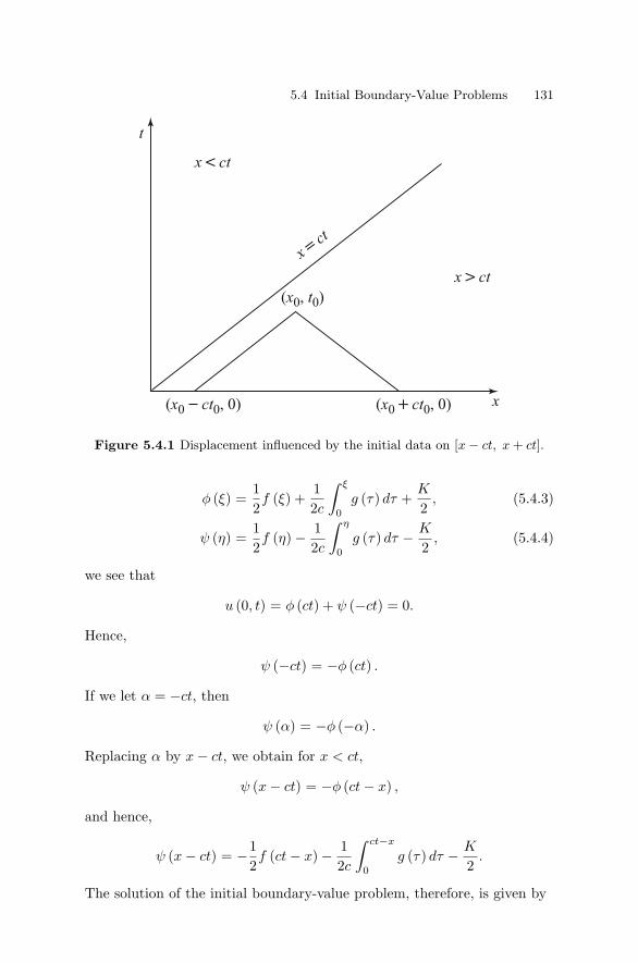
5.4 Initial Boundary-Value Problems 131
Figure 5.4.1 Displacement influenced by the initial data on [x − ct, x + ct].
φ (ξ) =12f (ξ) +
12c
∫ ξ
0g (τ) dτ +
K
2, (5.4.3)
ψ (η) =12f (η) − 1
2c
∫ η
0g (τ) dτ − K
2, (5.4.4)
we see that
u (0, t) = φ (ct) + ψ (−ct) = 0.
Hence,
ψ (−ct) = −φ (ct) .
If we let α = −ct, then
ψ (α) = −φ (−α) .
Replacing α by x − ct, we obtain for x < ct,
ψ (x − ct) = −φ (ct − x) ,
and hence,
ψ (x − ct) = −12f (ct − x) − 1
2c
∫ ct−x
0g (τ) dτ − K
2.
The solution of the initial boundary-value problem, therefore, is given by

132 5 The Cauchy Problem and Wave Equations
u (x, t) =12
[f (x + ct) + f (x − ct)] +12c
∫ x+ct
x−ct
g (τ) dτ for x > ct, (5.4.5)
u (x, t) =12
[f (x + ct) − f (ct − x)] +12c
∫ x+ct
ct−x
g (τ) dτ for x < ct. (5.4.6)
In order for this solution to exist, f must be twice continuously differ-entiable and g must be continuously differentiable, and in addition
f (0) = f ′′ (0) = g (0) = 0.
Solution (5.4.6) has an interesting physical interpretation. If we drawthe characteristics through the point (x0, t0) in the region x > ct, we see,as pointed out earlier, that the displacement at (x0, t0) is determined bythe initial values on [x0 − ct0, x0 + ct0].
If the point (x0, t0) lies in the region x > ct as shown in Figure 5.4.1,we see that the characteristic x + ct = x0 + ct0 intersects the x-axis at(x0 + ct0, 0). However, the characteristic x − ct = x0 − ct0 intersects thet-axis at (0, t0 − x0/c), and the characteristic x + ct = ct0 − x0 intersectsthe x-axis at (ct0 − x0, 0). Thus, the disturbance at (ct0 − x0, 0) travelsalong the backward characteristic x + ct = ct0 − x0, and is reflected at(0, t0 − x0/c) as a forward moving wave represented by −φ (ct0 − x0).
Example 5.4.1. Determine the solution of the initial boundary-value prob-lem
utt = 4uxx, x > 0, t > 0,
u (x, 0) = |sin x| , x > 0,
ut (x, 0) = 0, x ≥ 0,
u (x, 0) = 0, t ≥ 0.
For x > 2t,
u (x, t) =12
[f (x + 2t) + f (x − 2t)]
=12
[|sin (x + 2t)| − |sin (x − 2t)|] ,
and for x < 2t,
u (x, t) =12
[f (x + 2t) − f (2t − x)]
=12
[|sin (x + 2t)| − |sin (2t − x)|] .
Notice that u (0, t) = 0 is satisfied by u (x, t) for x < 2t (that is, t > 0).

5.4 Initial Boundary-Value Problems 133
(B) Semi-infinite String with a Free EndWe consider a semi-infinite string with a free end at x = 0. We will
determine the solution of
utt = c2uxx, 0 < x < ∞, t > 0,
u (x, 0) = f (x) , 0 ≤ x < ∞, (5.4.7)ut (x, 0) = g (x) , 0 ≤ x < ∞,
ux (0, t) = 0, 0 ≤ t < ∞.
As in the case of the fixed end, for x > ct the solution is the same asthat of the infinite string. For x < ct, from the d’Alembert solution (5.4.2)
u (x, t) = φ (x + ct) + ψ (x − ct) ,
we have
ux (x, t) = φ′ (x + ct) + ψ′ (x − ct) .
Thus,
ux (0, t) = φ′ (ct) + ψ′ (−ct) = 0.
Integration yields
φ (ct) − ψ (−ct) = K,
where K is a constant. Now, if we let α = −ct, we obtain
ψ (α) = φ (−α) − K.
Replacing α by x − ct, we have
ψ (x − ct) = φ (ct − x) − K,
and hence,
ψ (x − ct) =12
f (ct − x) +12c
∫ ct−x
0g (τ) dτ − K
2.
The solution of the initial boundary-value problem, therefore, is given by
u (x, t) =12
[f (x + ct) + f (x − ct)] +12c
∫ x+ct
x−ct
g (τ) dτ for x > ct. (5.4.8)
u (x, t) =12
[f (x + ct) + f (ct − x)] +12c
[∫ x+ct
0g (τ) dτ +
∫ ct−x
0g (τ) dτ
]for x < ct. (5.4.9)
We note that for this solution to exist, f must be twice continuouslydifferentiable and g must be continuously differentiable, and in addition,
f ′ (0) = g′ (0) = 0.

134 5 The Cauchy Problem and Wave Equations
Example 5.4.2. Find the solution of the initial boundary-value problem
utt = uxx, 0 < x < ∞, t > 0,
u (x, 0) = cos(πx
2
), 0 ≤ x < ∞,
ut (x, 0) = 0, 0 ≤ x < ∞,
ux (x, 0) = 0, t ≥ 0.
For x > t
u (x, t) =12
[cos
π
2(x + t) + cos
π
2(x − t)
]= cos
(π
2x)
cos(π
2t)
,
and for x < t
u (x, t) =12
[cos
π
2(x + t) + cos
π
2(t − x)
]= cos
(π
2x)
cos(π
2t)
.
5.5 Equations with Nonhomogeneous BoundaryConditions
In the case of the initial boundary-value problems with nonhomogeneousboundary conditions, such as
utt = c2uxx, x > 0, t > 0,
u (x, 0) = f (x) , x ≥ 0, (5.5.1)ut (x, 0) = g (x) , x ≥ 0,
u (0, t) = p (t) , t ≥ 0,
we proceed in a manner similar to the case of homogeneous boundary con-ditions. Using equation (5.4.2), we apply the boundary condition to obtain
u (0, t) = φ (ct) + ψ (−ct) = p (t) .
If we let α = −ct, we have
ψ (α) = p(−α
c
)− φ (−α) .
Replacing α by x − ct, the preceding relation becomes
ψ (x − ct) = p(t − x
c
)− φ (ct − x) .
5.5 Equations with Nonhomogeneous Boundary Conditions 135
Thus, for 0 ≤ x < ct,
u (x, t) = p(t − x
c
)+
12
[f (x + ct) − f (ct − x)] +12c
∫ x+ct
ct−x
g (τ) dτ
= p(t − x
c
)+ φ (x + ct) − ψ (ct − x) , (5.5.2)
where φ (x + ct = ξ) is given by (5.3.11), and ψ (η) is given by
ψ (η) =12f (η) +
12c
∫ η
0g (τ) dτ. (5.5.3)
The solution for x > ct is given by the solution (5.4.5) of the infinite string.In this case, in addition to the differentiability conditions satisfied by
f and g, as in the case of the problem with the homogeneous boundaryconditions, p must be twice continuously differentiable in t and
p (0) = f (0) , p′ (0) = g (0) , p′′ (0) = c2f ′′ (0) .
We next consider the initial boundary-value problem
utt = c2uxx, x > 0, t > 0,
u (x, 0) = f (x) , x ≥ 0,
ut (x, 0) = g (x) , x ≥ 0,
ux (0, t) = q (t) , t ≥ 0.
Using (5.4.2), we apply the boundary condition to obtain
ux (0, t) = φ′ (ct) + ψ′ (−ct) = q (t) .
Then, integrating yields
φ (ct) − ψ (−ct) = c
∫ t
0q (τ) dτ + K.
If we let α = −ct, then
ψ (α) = φ (−α) − c
∫ −α/c
0q (τ) dτ − K.
Replacing α by x − ct, we obtain
ψ (x − ct) = φ (ct − x) − c
∫ t−x/c
0q (τ) dτ − K.
The solution of the initial boundary-value problem for x < ct, therefore, isgiven by

136 5 The Cauchy Problem and Wave Equations
u (x, t) =12
[f (x + ct) + f (ct − x)] +12c
[∫ x+ct
0g (τ) dτ +
∫ ct−x
0g (τ) dτ
]−c
∫ t−x/c
0q (τ) dτ. (5.5.4)
Here f and g must satisfy the differentiability conditions, as in the case ofthe problem with the homogeneous boundary conditions. In addition
f ′ (0) = q (0) , g′ (0) = q′ (0) .
The solution for the initial boundary-value problem involving the bound-ary condition
ux (0, t) + hu (0, t) = 0, h = constant
can also be constructed in a similar manner from the d’Alembert solution.
5.6 Vibration of Finite String with Fixed Ends
The problem of the finite string is more complicated than that of the infinitestring due to the repeated reflection of waves from the boundaries
We first consider the vibration of the string of length l fixed at bothends. The problem is that of finding the solution of
utt = c2uxx, 0 < x < l, t > 0,
u (x, 0) = f (x) , 0 ≤ x ≤ l,
ut (x, 0) = g (x) , 0 ≤ x ≤ l, (5.6.1)u (0, t) = 0, u (l, t) = 0, t ≥ 0,
From the previous results, we know that the solution of the wave equa-tion is
u (x, t) = φ (x + ct) + ψ (x − ct) .
Applying the initial conditions, we have
u (x, 0) = φ (x) + ψ (x) = f (x) , 0 ≤ x ≤ l,
ut (x, 0) = c φ′ (x) − c ψ′ (x) = g (x) , 0 ≤ x ≤ l.
Solving for φ and ψ, we find
φ (ξ) =12f (ξ) +
12c
∫ ξ
0g (τ) dτ +
K
2, 0 ≤ ξ ≤ l, (5.6.2)
ψ (η) =12f (η) − 1
2c
∫ η
0g (τ) dτ − K
2, 0 ≤ η ≤ l. (5.6.3)

5.6 Vibration of Finite String with Fixed Ends 137
Hence,
u (x, t) =12
[f (x + ct) + f (x − ct)] +12c
∫ x+ct
x−ct
g (τ) dτ, (5.6.4)
for 0 ≤ x + ct ≤ l and 0 ≤ x − ct ≤ l. The solution is thus uniquelydetermined by the initial data in the region
t ≤ x
c, t ≤ l − x
c, t ≥ 0.
For larger times, the solution depends on the boundary conditions. Applyingthe boundary conditions, we obtain
u (0, t) = φ (ct) + ψ (−ct) = 0, t ≥ 0, (5.6.5)u (l, t) = φ (l + ct) + ψ (l − ct) = 0, t ≥ 0. (5.6.6)
If we set α = −ct, equation (5.6.5) becomes
ψ (α) = −φ (−α) , α ≤ 0, (5.6.7)
and if we set α = l + ct, equation (5.6.6) takes the form
φ (α) = −ψ (2l − α) , α ≥ l. (5.6.8)
With ξ = −η, we may write equation (5.6.2) as
φ (−η) =12f (−η) +
12c
∫ −η
0g (τ) dτ +
K
2, 0 ≤ −η ≤ l. (5.6.9)
Thus, from (5.6.7) and (5.6.9), we have
ψ (η) = −12f (−η) − 1
2c
∫ −η
0g (τ) dτ − K
2, −l ≤ η ≤ 0. (5.6.10)
We see that the range of ψ (η) is extended to −l ≤ η ≤ l.If we put α = ξ in equation (5.6.8), we obtain
φ (ξ) = −ψ (2l − ξ) , ξ ≥ l. (5.6.11)
Then, by putting η = 2l − ξ in equation (5.6.3), we obtain
ψ (2l − ξ) =12
f (2l − ξ) − 12c
∫ 2l−ξ
0g (τ) dτ − K
2, 0 ≤ 2l − ξ ≤ l.
(5.6.12)
Substitution of this in equation (5.6.11) yields

138 5 The Cauchy Problem and Wave Equations
φ (ξ) = −12f (2l − ξ) +
12c
∫ 2l−ξ
0g (τ) dτ +
K
2, l ≤ ξ ≤ 2l. (5.6.13)
The range of φ (ξ) is thus extended to 0 ≤ ξ ≤ 2l. Continuing in thismanner, we obtain φ (ξ) for all ξ ≥ 0 and ψ (η) for all η ≤ l. Hence, thesolution is determined for all 0 ≤ x ≤ l and t ≥ 0.
In order to observe the effect of the boundaries on the propagation ofwaves, the characteristics are drawn through the end point until they meetthe boundaries and then continue inward as shown in Figure 5.6.1. It can beseen from the figure that only direct waves propagate in region 1. In regions2 and 3, both direct and reflected waves propagate. In regions, 4,5,6, ... ,several waves propagate along the characteristics reflected from both of theboundaries x = 0 and x = l.
Example 5.6.1. Determine the solution of the following problem
utt = c2uxx, 0 < x < l, t > 0,
u (x, 0) = sin (πx/l) , 0 ≤ x ≤ l,
ut (x, 0) = 0, 0 ≤ x ≤ l,
u (0, t) = 0, u (l, t) = 0, t ≥ 0.
From equations (5.6.2) and (5.6.3), we have
Figure 5.6.1 Regions of wave propagation.

5.7 Nonhomogeneous Wave Equations 139
φ (ξ) =12
sin(
πξ
l
)+
K
2, 0 ≤ ξ ≤ l.
ψ (η) =12
sin(πη
l
)− K
2, 0 ≤ η ≤ l.
Using equation (5.6.10), we obtain
ψ (η) = −12
sin(−πη
l
)− K
2, −l ≤ η ≤ 0
=12
sin(πη
l
)− K
2.
From equation (5.6.13), we find
φ (ξ) = −12
sinπ
l(2l − ξ)
+
K
2, l ≤ ξ ≤ 2l.
Again by equation (5.6.7) and from the preceding φ (ξ), we have
φ (η) =12
sin(πη
l
)− K
2, −2l ≤ η ≤ −l.
Proceeding in this manner, we determine the solution
u (x, t) = φ (ξ) + ψ (η)
=12
[sin
π
l(x + ct) + sin
π
l(x − ct)
]for all x in (0, l) and for all t > 0.
Similarly, the solution of the finite initial boundary-value problem
utt = c2uxx, 0 < x < l, t > 0,
u (x, 0) = f (x) , 0 ≤ x ≤ l,
ut (x, 0) = g (x) , 0 ≤ x ≤ l,
u (0, t) = p (t) , u (l, t) = q (t) , t ≥ 0,
can be determined by the same method.
5.7 Nonhomogeneous Wave Equations
We shall consider next the Cauchy problem for the nonhomogeneous waveequation
utt = c2uxx + h∗ (x, t) , (5.7.1)
with the initial conditions
u (x, 0) = f (x) , ut (x, 0) = g∗ (x) . (5.7.2)

140 5 The Cauchy Problem and Wave Equations
By the coordinate transformation
y = ct, (5.7.3)
the problem is reduced to
uxx − uyy = h (x, y) , (5.7.4)u (x, 0) = f (x) , (5.7.5)
uy (x, 0) = g (x) , (5.7.6)
where h (x, y) = −h∗/c2 and g (x) = g∗/c.
Let P0 (x0, y0) be a point of the plane, and let Q0 be the point (x0, 0)on the initial line y = 0. Then the characteristics, x+ y = constant, ofequation (5.7.4) are two straight lines drawn through the point P0 withslopes + 1. Obviously, they intersect the x-axis at the points P1 (x0 − y0, 0)and P2 (x0 + y0, 0), as shown in Figure 5.7.1. Let the sides of the triangleP0P1P2 be designated by B0, B1, and B2, and let D be the region repre-senting the interior of the triangle and its boundaries B. Integrating bothsides of equation (5.7.4), we obtain∫∫
R
(uxx − uyy) dR =∫∫
R
h (x, y) dR. (5.7.7)
Now we apply Green’s theorem to obtain
Figure 5.7.1 Triangular Region.

5.7 Nonhomogeneous Wave Equations 141∫∫R
(uxx − uyy) dR =∮
B
(uxdy + uydx) . (5.7.8)
Since B is composed of B0, B1, and B2, we note that∫B0
(ux dy + uy dx) =∫ x0+y0
x0−y0
uy dx,∫B1
(ux dy + uy dx) =∫
B1
(−ux dx − uy dy) ,
= u (x0 + y0, 0) − u (x0, y0) ,∫B2
(ux dy + uy dx) =∫
B2
(ux dx + uy dy) ,
= u (x0 − y0, 0) − u (x0, y0) .
Hence, ∮B
(ux dy + uy dx) = −2 u (x0, y0) + u (x0 − y0, 0)
+u (x0 + y0, 0) +∫ x0+y0
x0−y0
uy dx. (5.7.9)
Combining equations (5.7.7), (5.7.8) and (5.7.9), we obtain
u (x0, y0) =12
[u (x0 + y0, 0) + u (x0 − y0, 0)]
+12
∫ x0+y0
x0−y0
uy dx − 12
∫∫R
h (x, y) dR. (5.7.10)
We have chosen x0, y0 arbitrarily, and as a consequence, we replace x0 byx and y0 by y. Equation (5.7.10) thus becomes
u (x, y) =12
[f (x + y) + f (x − y)] +12
∫ x+y
x−y
g (τ) dτ − 12
∫∫R
h (x, y) dR.
In terms of the original variables
u (x, t) =12
[f (x + ct) + f (x − ct)] +12c
∫ x+ct
x−ct
g∗ (τ) dτ − 12
∫∫R
h (x, t) dR.
(5.7.11)
Example 5.7.1. Determine the solution of
uxx − uyy = 1,
u (x, 0) = sinx,
uy (x, 0) = x.

142 5 The Cauchy Problem and Wave Equations
Figure 5.7.2 Triangular Region.
It is easy to see that the characteristics are x+ y = constant = x0 + y0 andx − y = constant = x0 − y0, as shown in Figure 5.7.2. Thus,
u (x0, y0) =12
[sin (x0 + y0) + sin (x0 − y0)]
+12
∫ x0+y0
x0−y0
τ dτ − 12
∫ y0
0
∫ −y+x0+y0
y+x0−y0
dx dy
=12
[sin (x0 + y0) + sin (x0 − y0)] + x0y0 − 12
y20 .
Now dropping the subscript zero, we obtain the solution
u (x, y) =12
[sin (x + y) + sin (x − y)] + xy − 12
y2.
5.8 The Riemann Method
We shall discuss Riemann’s method of integrating the linear hyperbolicequation
L [u] ≡ uxy + aux + buy + cu = f (x, y) , (5.8.1)

5.8 The Riemann Method 143
where L denotes the linear operator, and a (x, y), b (x, y), c (x, y), andf (x, y) are differentiable functions in some domain D∗. The method con-sists essentially of the derivation of an integral formula which representsthe solution of the Cauchy problem.
Let v (x, y) be a function having continuous second-order partial deriva-tives. Then, we may write
vuxy − uvxy = (vux)y − (vuy)x ,
vaux = (avu)x − u (av)x , (5.8.2)vbuy = (bvu)y − u (bv)y ,
so that
vL [u] − uM [v] = Ux + Vy, (5.8.3)
where M is the operator represented by
M [v] = vxy − (av)x − (bv)y + cv, (5.8.4)
and
U = auv − uvy, V = buv + vux. (5.8.5)
The operator M is called the adjoint operator of L. If M = L, then theoperator L is said to be self-adjoint. Now applying Green’s theorem, wehave ∫∫
D
(Ux + Vy) dx dy =∮
C
(U dy − V dx) , (5.8.6)
where C is the closed curve bounding the region of integration D which isin D∗.
Let Λ be a smooth initial curve which is continuous, as shown in Figure5.8.1. Since equation (5.8.1) is in first canonical form, x and y are thecharacteristic coordinates. We assume that the tangent to Λ is nowhereparallel to the x or y axis. Let P (α, β) be a point at which the solution tothe Cauchy problem is sought. Line PQ parallel to the x axis intersects theinitial curve Λ at Q, and line PR parallel to the y axis intersects the curveΛ at R. We suppose that u and ux or uy are prescribed along Λ.
Let C be the closed contour PQRP bounding D. Since dy = 0 on PQand dx = 0 on PR, it follows immediately from equations (5.8.3) and (5.8.6)that∫∫
D
(vL [u] − uM [v]) dx dy =∫ R
Q
(U dy − V dx) +∫ P
R
U dy −∫ Q
P
V dx.
(5.8.7)

144 5 The Cauchy Problem and Wave Equations
Figure 5.8.1 Smooth initial curve.
From equation (5.8.5), we find∫ Q
P
V dx =∫ Q
P
bvu dx +∫ Q
P
vux dx.
Integrating by parts, we obtain∫ Q
P
vuxdx = [uv]QP −∫ Q
P
uvxdx.
Hence, we may write∫ Q
P
V dx = [uv]QP +∫ Q
P
u (bv − vx) dx.
Substitution of this integral in equation (5.8.7) yields
[uv]P = [uv]Q +∫ Q
P
u (bv − vx) dx −∫ P
R
u (av − vy) dy −∫ R
Q
(U dy − V dx)
+∫∫
D
(vL [u] − uM [v]) dx dy. (5.8.8)
Suppose we can choose the function v (x, y; α, β) to be the solution ofthe adjoint equation

5.8 The Riemann Method 145
M [v] = 0, (5.8.9)
satisfying the conditions
vx = bv when y = β,
vy = av when x = α, (5.8.10)v = 1 when x = α and y = β.
The function v (x, y; α, β) is called the Riemann function. Since L [u] = f ,equation (5.8.8) reduces to,
[u]P = [uv]Q −∫ R
Q
uv (a dy − b dx) +∫ R
Q
(uvydy + vuxdx) +∫∫
D
vf dx dy.
(5.8.11)
This gives us the value of u at the point P when u and ux are prescribedalong the curve Λ. When u and uy are prescribed, the identity
[uv]R − [uv]Q =∫ R
Q
(uv)x dx + (uv)y dy
,
may be used to put equation (5.8.8) in the form
[u]P = [uv]R −∫ R
Q
uv (a dy − b dx) −∫ R
Q
(uvxdx + vuydy)
+∫∫
D
vf dx dy. (5.8.12)
By adding equations (5.8.11) and (5.8.12), the value of u at P is given by
[u]P =12
([uv]Q + [uv]R
)−
∫ R
Q
uv (a dy − b dx) − 12
∫ R
Q
u (vxdx − vydy)
+12
∫ R
Q
v (uxdx − uydy) +∫∫
D
vf dx dy (5.8.13)
which is the solution of the Cauchy problem in terms of the Cauchy datagiven along the curve Λ. It is easy to see that the solution at the point(α, β) depends only on the Cauchy data along the arc QR on Λ. If theinitial data were to change outside this arc QR, the solution would changeonly outside the triangle PQR. Thus, from Figure 5.8.2, we can see thateach characteristic separates the region in which the solution remains un-changed from the region in which it varies. Because of this fact, the uniquecontinuation of the solution across any characteristic is not possible. Thisis evident from Figure 5.8.2. The solution on the right of the characteristicP1R1 is determined by the initial data given in Q1R2, whereas the solution

146 5 The Cauchy Problem and Wave Equations
Figure 5.8.2 Solution on the right and left of the characteristic.
on the left is determined by the initial data given on Q1R1. If the initialdata on R1R2 were changed, the solution on the right of P1R1 only will beaffected.
It should be remarked here that the initial curve can intersect eachcharacteristic at only one point. Suppose, for example, the initial curve Λintersects the characteristic at two points, as shown in Figure 5.8.3. Then,the solution at P obtained from the initial data on QR will be differentfrom the solution obtained from the initial data on RS. Hence, the Cauchyproblem, in this case, is not solvable.
Figure 5.8.3 Initial curve intersects the characteristic at two points.

5.8 The Riemann Method 147
Example 5.8.1. The telegraph equation
wtt + a∗wt + b∗w = c2wxx,
may be transformed into canonical form
L [u] = uξη + ku = 0,
by the successive transformations
w = u e−a∗t/2,
and
ξ = x + ct, η = x − ct,
where k =(a∗2 − 4b∗) /16c2.
We apply Riemann’s method to determine the solution satisfying theinitial conditions
u (x, 0) = f (x) , ut (x, 0) = g (x) .
Since
t =12c
(ξ − η) ,
the line t = 0 corresponds to the straight line ξ = η in the ξ − η plane. Theinitial conditions may thus be transformed into
[u]ξ=η = f (ξ) , (5.8.14)
[uξ − uη]ξ=η = c−1g (ξ) . (5.8.15)
We next determine the Riemann function v (ξ, η; α, β) which satisfies
vξη + kv = 0, (5.8.16)vξ (ξ, β; α, β) = 0, (5.8.17)vη (α, η; α, β) = 0, (5.8.18)v (α, β; α, β) = 1. (5.8.19)
The differential equation (5.8.16) is self-adjoint, that is,
L [v] = M [v] = vξη + kv.
We assume that the Riemann function is of the form
v (ξ, η; α, β) = F (s) ,
with the argument s = (ξ − α) (η − β). Substituting this value in equation(5.8.16), we obtain

148 5 The Cauchy Problem and Wave Equations
sFss + Fs + kF = 0.
If we let λ =√
4ks, the above equation becomes
F ′′ (λ) +1λ
F ′ (λ) + F (λ) = 0.
This is the Bessel equation of order zero, and the solution is
F (λ) = J0 (λ) ,
disregarding Y0 (λ) which is unbounded at λ = 0. Thus, the Riemann func-tion is
v (ξ, η; α, β) = J0
(√4k (ξ − α) (η − β)
)which satisfies equation (5.8.16) and is equal to one on the characteristicsξ = α and η = β. Since J ′
0 (0) = 0, equations (5.8.17) and (5.8.18) aresatisfied. From this, it immediately follows that
[vξ]ξ=η =
√k (ξ − β)√
(ξ − α) (η − β)[J ′
0 (λ)]ξ=η ,
[vη]ξ=η =
√k (ξ − α)√
(ξ − α) (η − β)[J ′
0 (λ)]ξ=η .
Thus, we have
[vξ − uη]ξ=η =
√k (α − β)√
(ξ − α) (ξ − β)[J ′
0 (λ)]ξ=η . (5.8.20)
From the initial condition
u (Q) = f (β) and u (R) = f (α) , (5.8.21)
and substituting equations (5.8.15), (5.8.19), and (5.8.20) into equation(5.8.13), we obtain
u (α, β) =12
[f (α) + f (β)]
−12
∫ α
β
√k (α − β)√
(τ − α) (τ − β)J ′
0
(√4k (τ − α) (τ − β)
)f (τ) dτ
+12c
∫ α
β
J0
(√4k (τ − α) (τ − β)
)g (τ) dτ. (5.8.22)
Replacing α and β by ξ and η, and substituting the original variables x andt, we obtain

5.9 Solution of the Goursat Problem 149
u (x, t) =12
[f (x + ct) + f (x − ct)] +12
∫ x+ct
x−ct
G (x, t, τ) dτ, (5.8.23)
where
G (x, t, τ)
=
−2
√k ctf (τ) J0
(√4k
[(τ − x)2 − c2t2
])/√(τ − x)2 − c2t2
+ c−1g (τ) J0
(√4k
[(τ − x)2 − c2t2
]).
If we set k = 0, we arrive at the d’Alembert solution for the wave equation
u (x, t) =12
[f (x + ct) + f (x − ct)] +12c
∫ x+ct
x−ct
g (τ) dτ.
5.9 Solution of the Goursat Problem
The Goursat problem is that of finding the solution of a linear hyperbolicequation
uxy = a1 (x, y) ux + a2 (x, y) uy + a3 (x, y) u + h (x, y) , (5.9.1)
satisfying the prescribed conditions
u (x, y) = f (x) , (5.9.2)
on a characteristic, say, y = 0, and
u (x, y) = g (x) (5.9.3)
on a monotonic increasing curve y = y (x) which, for simplicity, is assumedto intersect the characteristic at the origin.
The solution in the region between the x-axis and the monotonic curvein the first quadrant can be determined by the method of successive ap-proximations. The proof is given in Garabedian (1964).
Example 5.9.1. Determine the solution of the Goursat problem
utt = c2uxx, (5.9.4)u (x, t) = f (x) , on x − ct = 0, (5.9.5)u (x, t) = g (x) , on t = t (x) , (5.9.6)
where f (0) = g (0).

150 5 The Cauchy Problem and Wave Equations
The general solution of the wave equation is
u (x, t) = φ (x + ct) + ψ (x − ct) .
Applying the prescribed conditions, we obtain
f (x) = φ (2x) + ψ (0) , (5.9.7)g (x) = φ (x + c t (x)) + ψ (x − c t (x)) . (5.9.8)
It is evident that
f (0) = φ (0) + ψ (0) = g (0) .
Now, if s = x − c t (x), the inverse of it is x = α (s). Thus, equation (5.9.8)may be written as
g (α (s)) = φ (x + c t (x)) + ψ (s) . (5.9.9)
Replacing x by (x + c t (x)) /2 in equation (5.9.7), we obtain
f
(x + c t (x)
2
)= φ (x + c t (x)) + ψ (0) . (5.9.10)
Thus, using (5.9.10), equation (5.9.9) becomes
ψ (s) = g (α (s)) − f
(α (s) + c t (α (s))
2
)+ ψ (0) .
Replacing s by x − ct , we have
ψ (x − ct) = g (α (x − ct)) − f
(α (x − c t) + c t (α (x − c t))
2
)+ ψ (0) .
Hence, the solution is given by
u (x, t) = f
(x + c t
2
)− f
(α (x − c t) + c t (α (x − c t))
2
)+ g (α (x − c t)) .
(5.9.11)
Let us consider a special case when the curve t = t (x) is a straight linerepresented by t − kx = 0 with a constant k > 0. Then s = x − ckx andhence x = s/ (1 − ck). Using these values in (5.9.11), we obtain
u (x, t) = f
(x + c t
2
)− f
((1 + c k) (x − c t)
2 (1 − c k)
)+ g
(x − c t
1 − c k
). (5.9.12)
When the values of u are prescribed on both characteristics, the problemof finding u of a linear hyperbolic equation is called a characteristic initial-value problem. This is a degenerate case of the Goursat problem.

5.9 Solution of the Goursat Problem 151
Consider the characteristic initial-value problem
uxy = h (x, y) , (5.9.13)u (x, 0) = f (x) , (5.9.14)u (0, y) = g (y) , (5.9.15)
where f and g are continuously differentiable, and f (0) = g (0).Integrating equation (5.9.13), we obtain
u (x, y) =∫ x
0
∫ y
0h (ξ, η) dη dξ + φ (x) + ψ (y) , (5.9.16)
where φ and ψ are arbitrary functions. Applying the prescribed conditions(5.9.14) and (5.9.15), we have
u (x, 0) = φ (x) + ψ (0) = f (x) , (5.9.17)u (0, y) = φ (0) + ψ (y) = g (y) . (5.9.18)
Thus,
φ (x) + ψ (y) = f (x) + g (y) − φ (0) − ψ (0) . (5.9.19)
But from (5.9.17), we have
φ (0) + ψ (0) = f (0) . (5.9.20)
Hence, from (5.9.16), (5.9.19) and (5.9.20), we obtain
u (x, y) = f (x) + g (y) − f (0) +∫ x
0
∫ y
0h (ξ, η) dη dξ. (5.9.21)
Example 5.9.2. Determine the solution of the characteristic initial-valueproblem
utt = c2uxx,
u (x, t) = f (x) on x + ct = 0,
u (x, t) = g (x) on x − ct = 0,
where f (0) = g (0).Here it is not necessary to reduce the given equation to canonical form.
The general solution of the wave equation is
u (x, t) = φ (x + ct) + ψ (x − ct) .
The characteristics are
x + ct = 0, x − ct = 0.

152 5 The Cauchy Problem and Wave Equations
Applying the prescribed conditions, we have
u (x, t) = φ (2x) + ψ (0) = f (x) on x + ct = 0, (5.9.22)u (x, t) = φ (0) + ψ (2x) = g (x) on x − ct = 0. (5.9.23)
We observe that these equations are compatible, since f (0) = g (0).Now, replacing x by (x + ct) /2 in equation (5.9.22) and replacing x by
(x − ct) /2 in equation (5.9.23), we have
φ (x + ct) = f
(x + ct
2
)− ψ (0) ,
φ (x − ct) = g
(x − ct
2
)− φ (0) .
Hence, the solution is given by
u (x, t) = f
(x + ct
2
)+ g
(x − ct
2
)− f (0) . (5.9.24)
We note that this solution can be obtained by substituting k = −1/c into(5.9.12).
Example 5.9.3. Find the solution of the characteristic initial-value problem
y3uxx − yuyy + uy = 0, (5.9.25)
u (x, y) = f (x) on x +y2
2= 4 for 2 ≤ x ≤ 4,
u (x, y) = g (x) on x − y2
2= 0 for 0 ≤ x ≤ 2,
with f (2) = g (2).Since the equation is hyperbolic except for y = 0, we reduce it to the
canonical form
uξη = 0,
where ξ = x +(y2/2
)and η = x − (
y2/2). Thus, the general solution is
u (x, y) = φ
(x +
y2
2
)+ ψ
(x − y2
2
). (5.9.26)
Applying the prescribed conditions, we have
f (x) = φ (4) + ψ (2x − 4) , (5.9.27)g (x) = φ (2x) + ψ (0) . (5.9.28)
Now, if we replace (2x − 4) by(x − y2/2
)in (5.9.27) and (2x) by
(x + y2/2
)in (5.9.28), we obtain

5.10 Spherical Wave Equation 153
ψ
(x − y2
2
)= f
(x
2− y2
4+ 2
)− φ (4) ,
φ
(x +
y2
2
)= g
(x
2+
y2
4
)− ψ (0) .
Thus,
u (x, y) = f
(x
2− y2
4+ 2
)+ g
(x
2+
y2
4
)− φ (4) − ψ (0) .
But from (5.9.27) and (5.9.28), we see that
f (2) = φ (4) + ψ (0) = g (2) .
Hence,
u (x, y) = f
(x
2− y2
4+ 2
)+ g
(x
2+
y2
4
)− f (2) .
5.10 Spherical Wave Equation
In spherical polar coordinates (r, θ, φ), the wave equation (3.1.1) takes theform
1r2
∂
∂r
(r2 ∂u
∂r
)+
1r2 sin θ
∂
∂θ
(sin θ
∂u
∂θ
)+
1r2 sin2 θ
∂2u
∂φ2 =1c2
∂2u
∂t2.(5.10.1)
Solutions of this equation are called spherical symmetric waves if udepends on r and t only. Thus, the solution u = u (r, t) which satisfies thewave equation with spherical symmetry in three-dimensional space is
1r2
∂
∂r
(r2 ∂u
∂r
)=
1c2
∂2u
∂t2. (5.10.2)
Introducing a new dependent variable U = ru (r, t), this equation re-duces to a simple form
Utt = c2Urr. (5.10.3)
This is identical with the one-dimensional wave equation (5.3.1) and hasthe general solution in the form
U (r, t) = φ (r + ct) + ψ (r − ct) , (5.10.4)
or, equivalently,
u (r, t) =1r
[φ (r + ct) + ψ (r − ct)] . (5.10.5)

154 5 The Cauchy Problem and Wave Equations
This solution consists of two progressive spherical waves traveling withconstant velocity c. The terms involving φ and ψ represent the incomingwaves to the origin and the outgoing waves from the origin respectively.
Physically, the solution for only outgoing waves generated by a sourceis of most interest, and has the form
u (r, t) =1r
ψ (r − ct) , (5.10.6)
where the explicit form of ψ is to be determined from the properties of thesource. In the context of fluid flows, u represents the velocity potential sothat the limiting total flux through a sphere of center at the origin andradius r is
Q (t) = limr→0
4πr2ur (r, t) = −4π ψ (−ct) . (5.10.7)
In physical terms, we say that there is a simple (or monopole) point sourceof strength Q (t) located at the origin. Thus, the solution (5.10.6) can beexpressed in terms of Q as
u (r, t) = − 14πr
Q(t − r
c
). (5.10.8)
This represents the velocity potential of the point source, and ur is calledthe radial velocity. In fluid flows, the difference between the pressure at anytime t and the equilibrium value is given by
p − p0 = ρ ut = − ρ
4πrQ
(t − r
c
), (5.10.9)
where ρ is the density of the fluid.Following an analysis similar to Section 5.3, the solution of the initial-
value problem with the initial data
u (r, 0) = f (r) , ut (r, 0) = g (r) , r ≥ 0, (5.10.10)
where f and g are continuously differentiable, is given by
u (r, t) =12r
[(r + ct) f (r + ct) + (r − ct) f (r − ct) +
1c
∫ r+ct
r−ct
τg (τ) dτ
],
(5.10.11)
provided r ≥ ct. However, when r < ct, this solution fails because f and gare not defined for r < 0. This initial data at t = 0, r ≥ 0 determine thesolution u (r, t) only up to the characteristic r = ct in the r-t plane. To findu for r < ct, we require u to be finite at r = 0 for all t ≥ 0, that is, U = 0at r = 0. Thus, the solution for U (r, t) is

5.11 Cylindrical Wave Equation 155
U (r, t) =12
[(r + ct) f (r + ct) + (r − ct) f (r − ct) +
1c
∫ r+ct
r−ct
τg (τ) dτ
],
(5.10.12)
provided r ≥ ct ≥ 0, and
U (r, t) =12
[φ (ct + r) + ψ (ct − r)] , ct ≥ r ≥ 0, (5.10.13)
where
φ (ct) + ψ (ct) = 0, for ct ≥ 0. (5.10.14)
In view of the fact that Ur + 1c Ut is constant on each characteristic
r + ct = constant, it turns out that
φ′ (ct + r) = (r + ct) f ′ (r + ct) + f (r + ct) +1c
(r + ct) g (r + ct) ,
or
φ′ (ct) = ctf ′ (ct) + f (ct) + t g (ct) .
Integration gives
φ (t) = tf (t) +1c
∫ t
0τg (τ) dτ + φ (0) ,
so that
ψ (t) = −tf (t) − 1c
∫ t
0τg (τ) dτ − φ (0) .
Substituting these values into (5.10.13) and using U (r, t) = ru (r, t), weobtain, for ct > r,
u (r, t) =12r
[(ct + r) f (ct + r) − (ct − r) f (ct − r) +
1c
∫ ct+r
ct−r
τg (τ) dτ
].
(5.10.15)
5.11 Cylindrical Wave Equation
In cylindrical polar coordinates (R, θ, z), the wave equation (3.1.1) assumesthe form
uRR +1R
uR +1
R2 uθθ + uzz =1c2 utt. (5.11.1)
If u depends only on R and t, this equation becomes

156 5 The Cauchy Problem and Wave Equations
uRR +1R
uR =1c2 utt. (5.11.2)
Solutions of (5.11.2) are called cylindrical waves.In general, it is not easy to find the solution of (5.11.1). However, we
shall solve this equation by using the method of separation of variables inChapter 7. Here we derive the solution for outgoing cylindrical waves fromthe spherical wave solution (5.10.8). We assume that sources of constantstrength Q (t) per unit length are distributed uniformly on the z-axis. Thesolution for the cylindrical waves produced by the line source is given bythe total disturbance
u (R, t) = − 14π
∫ ∞
−∞
1r
Q(t − r
c
)dz = − 1
2π
∫ ∞
0
1r
Q(t − r
c
)dz, (5.11.3)
where R is the distance from the z-axis so that R2 =(r2 − z2
).
Substitution of z = R sinh ξ and r = R cosh ξ in (5.11.3) gives
u (R, t) = − 12π
∫ ∞
0Q
(t − R
ccosh ξ
)dξ. (5.11.4)
This is usually considered as the cylindrical wave function due to a sourceof strength Q (t) at R = 0. It follows from (5.11.4) that
utt = − 12π
∫ ∞
0Q′′
(t − R
ccosh ξ
)dξ, (5.11.5)
uR =1
2πc
∫ ∞
0cosh ξ Q′
(t − R
ccosh ξ
)dξ, (5.11.6)
uRR = − 12πc2
∫ ∞
0cosh2 ξ Q′′
(t − R
ccosh ξ
)dξ, (5.11.7)
which give
c2(
uRR +1R
uR
)− utt =
12π
∫ ∞
0
d
dξ
[c
RQ′
(t − R
ccosh ξ
)sinh ξ
]dξ
= limξ→∞
[c
2πRQ′
(t − R
ccosh ξ
)sinh ξ
]= 0,
provided the differentiation under the sign of integration is justified and theabove limit is zero. This means that u (R, t) satisfies the cylindrical waveequation (5.11.2).
In order to find the asymptotic behavior of the solution as R → 0, wesubstitute cosh ξ = c(t−ζ)
R into (5.11.4) and (5.11.6) to obtain
u = − 12π
∫ t−R/c
−∞
Q (ζ) dζ[(t − ζ)2 − R2
c2
] 12, (5.11.8)
uR =12π
∫ t−R/c
−∞
(t − ζ
R
)Q′ (ζ) dζ[
(t − ζ)2 − R2
c2
] 12, (5.11.9)

5.11 Cylindrical Wave Equation 157
which, in the limit R → 0, give
uR ∼ 12πR
∫ t
−∞Q′ (ζ) dζ =
12πR
Q (t) . (5.11.10)
This leads to the result
limR→0
2πR uR = Q (t) , (5.11.11)
or
u (R, t) ∼ 12π
Q (t) log R as R → 0. (5.11.12)
We next investigate the nature of the cylindrical wave solution near thewaterfront (R = ct) and in the far field (R → ∞). We assume Q (t) = 0 fort < 0 so that the lower limit of integration in (5.11.8) may be taken to bezero, and the solution is non-zero for τ = t − R
c > 0, where τ is the timepassed after the arrival of the wavefront. Consequently, (5.11.8) becomes
u (R, t) = − 12π
∫ τ
0
Q (ζ) dζ[(t − ζ)
(t − ζ + 2R
c
)] 12. (5.11.13)
Since 0 < ζ < τ , 2Rc > R
c > τ > τ − ζ > 0, so that the second factor underthe radical is approximately equal to 2R
c when R cτ , and hence,
u (R, t) ∼ − 12π
( c
2R
) 12∫ τ
0
Q (ζ) dζ
(t − ζ)12
= −( c
2R
) 12
q (τ)
= −( c
2R
) 12
q
(t − R
c
), R ct
2, (5.11.14)
where
q (τ) =12π
∫ τ
0
Q (ζ) dζ√τ − ζ
. (5.11.15)
Evidently, the amplitude involved in the solution (5.11.14) decays likeR− 1
2 for large R (R → ∞).
Example 5.11.1. Determine the asymptotic form of the solution (5.11.4) fora harmonically oscillating source of frequency ω.
We take the source in the form Q (t) = q0 exp [−i (ω + iε) t], where ε ispositive and small so that Q (t) → 0 as t → −∞. The small imaginary partε of ω will make insignificant contributions to the solution at finite time asε → 0. Thus, the solution (5.11.4) becomes
u (R, t) = −( q0
2π
)e−iωt
∫ ∞
0exp
(iωR
ccosh ξ
)dξ
= −(
iq0
4
)e−iωtH
(1)0
(ωR
c
), (5.11.16)

158 5 The Cauchy Problem and Wave Equations
where H(1)0 (z) is the Hankel function given by
H(1)0 (z) =
2πi
∫ ∞
0exp (iz cosh ξ) dξ. (5.11.17)
In view of the asymptotic expansion of H(1)0 (z) in the form
H(1)0 (z) ∼
(2πz
) 12
exp[i(z − π
4
)], z → ∞, (5.11.18)
the asymptotic solution for u (R, t) in the limit(
ωRc
) → ∞ is
u (R, t) ∼ −(
iq0
4
)(2c
πωR
) 12
exp[−i
(ωt − ωR
c− π
4
)].
This represents the cylindrical wave propagating with constant velocity c.The amplitude of the wave decays like R− 1
2 as R → ∞.
Example 5.11.2. For a supersonic flow (M > 1) past a solid body of revo-lution, the perturbation potential Φ satisfies the cylindrical wave equation
ΦRR +1R
ΦR = N2Φxx, N2 = M2 − 1,
where R is the distance from the path of the moving body and x is thedistance from the nose of the body.
It follows from problem 12 in 3.9 Exercises that Φ satisfies the equation
Φyy + Φzz = N2 Φxx.
This represents a two-dimensional wave equation with x ↔ t and N2 ↔1c2 . For a body of revolution with (y, z) ↔ (R, θ), ∂
∂θ ≡ 0, the above equationreduces to the cylindrical wave equation
ΦRR +1R
ΦR =1c2 Φtt.
5.12 Exercises
1. Determine the solution of each of the following initial-value problems:
(a) utt − c2uxx = 0, u (x, 0) = 0, ut (x, 0) = 1.
(b) utt − c2uxx = 0, u (x, 0) = sinx, ut (x, 0) = x2.
(c) utt − c2uxx = 0, u (x, 0) = x3, ut (x, 0) = x.

5.12 Exercises 159
(d) utt − c2uxx = 0, u (x, 0) = cos x, ut (x, 0) = e−1.
(e) utt − c2uxx = 0, u (x, 0) = log(1 + x2
), ut (x, 0) = 2.
(f) utt − c2uxx = 0, u (x, 0) = x, ut (x, 0) = sinx.
2. Determine the solution of each of the following initial-value problems:
(a) utt − c2uxx = x, u (x, 0) = 0, ut (x, 0) = 3.
(b) utt − c2uxx = x + ct, u (x, 0) = x, ut (x, 0) = sinx.
(c) utt − c2uxx = ex, u (x, 0) = 5, ut (x, 0) = x2.
(d) utt − c2uxx = sinx, u (x, 0) = cos x, ut (x, 0) = 1 + x.
(e) utt − c2uxx = xet, u (x, 0) = sinx, ut (x, 0) = 0.
(f) utt − c2uxx = 2, u (x, 0) = x2, ut (x, 0) = cos x.
3. A gas which is contained in a sphere of radius R is at rest initially, andthe initial condensation is given by s0 inside the sphere and zero outsidethe sphere. The condensation is related to the velocity potential by
s (t) =(1/c2)ut,
at all times, and the velocity potential satisfies the wave equation
utt = ∇2u.
Determine the condensation s (t) for all t > 0.
4. Solve the initial-value problem
uxx + 2uxy − 3uyy = 0,
u (x, 0) = sinx, uy (x, 0) = x.
5. Find the longitudinal oscillation of a rod subject to the initial conditions
u (x, 0) = sinx,
ut (x, 0) = x.
6. By using the Riemann method, solve the following problems:
(a) sin2 µ φxx − cos2 µ φyy − (λ2 sin2 µ cos2 µ
)φ = 0,
φ (0, y) = f1 (y) , φ (x, 0) = g1 (x) ,
φx (0, y) = f2 (y) , φy (x, 0) = g2 (x) .

160 5 The Cauchy Problem and Wave Equations
(b) x2uxx − t2utt = 0,
u (x, t1) = f (x) , ut (x, t2) = g (x) .
7. Determine the solution of the initial boundary-value problem
utt = 4 uxx, 0 < x < ∞, t > 0,
u (x, 0) = x4, 0 ≤ x < ∞,
ut (x, 0) = 0, 0 ≤ x < ∞,
u (0, t) = 0, t ≥ 0.
8. Determine the solution of the initial boundary-value problem
utt = 9 uxx, 0 < x < ∞, t > 0,
u (x, 0) = 0, 0 ≤ x < ∞,
ut (x, 0) = x3, 0 ≤ x < ∞,
ux (0, t) = 0, t ≥ 0.
9. Determine the solution of the initial boundary-value problem
utt = 16 uxx, 0 < x < ∞, t > 0,
u (x, 0) = sinx, 0 ≤ x < ∞,
ut (x, 0) = x2, 0 ≤ x < ∞,
u (0, t) = 0, t ≥ 0.
10. In the initial boundary-value problem
utt = c2uxx, 0 < x < l, t > 0,
u (x, 0) = f (x) , 0 ≤ x ≤ l,
ut (x, 0) = g (x) , 0 ≤ x ≤ l,
u (0, t) = 0, t ≥ 0,
if f and g are extended as odd functions, show that u (x, t) is given bythe solution (5.4.5) for x > ct and solution (5.4.6) for x < ct.
11. In the initial boundary-value problem
utt = c2uxx, 0 < x < l, t > 0,
u (x, 0) = f (x) , 0 ≤ x ≤ l,
ut (x, 0) = g (x) , 0 ≤ x ≤ l,
ux (0, t) = 0, t ≥ 0,
if f and g are extended as even functions, show that u (x, t) is given bysolution (5.4.8) for x > ct, and solution (5.4.9) for x < ct.

5.12 Exercises 161
12. Determine the solution of the initial boundary-value problem
utt = c2uxx, 0 < x < ∞, t > 0,
u (x, 0) = f (x) , 0 ≤ x < ∞,
ut (x, 0) = 0, 0 ≤ x < ∞,
ux (0, t) + hu (0, t) = 0, t ≥ 0, h = constant.
State the compatibility condition of f .
13. Find the solution of the problem
utt = c2uxx, at < x < ∞, t > 0,
u (x, 0) = f (x) , 0 < x < ∞,
ut (x, 0) = 0, 0 < x < ∞,
u (at, t) = 0, t > 0,
where f (0) = 0 and a is constant.
14. Find the solution of the initial boundary-value problem
utt = uxx, 0 < x < 2, t > 0,
u (x, 0) = sin (πx/2) , 0 ≤ x ≤ 2,
ut (x, 0) = 0, 0 ≤ x ≤ 2,
u (0, t) = 0, u (2, t) = 0, t ≥ 0.
15. Find the solution of the initial boundary-value problem
utt = 4uxx, 0 < x < 1, t > 0,
u (x, 0) = 0, 0 ≤ x ≤ 1,
ut (x, 0) = x (1 − x) , 0 ≤ x ≤ 1,
u (0, t) = 0, u (1, t) = 0, t ≥ 0.
16. Determine the solution of the initial boundary-value problem
utt = c2uxx, 0 < x < l, t > 0,
u (x, 0) = f (x) , 0 ≤ x ≤ l,
ut (x, 0) = g (x) , 0 ≤ x ≤ l,
ux (0, t) = 0, ux (l, t) = 0, t ≥ 0,
by extending f and g as even functions about x = 0 and x = l.
17. Determine the solution of the initial boundary-value problem
utt = c2uxx, 0 < x < l, t > 0,
u (x, 0) = f (x) , 0 ≤ x ≤ l,
ut (x, 0) = g (x) , 0 ≤ x ≤ l,
u (0, t) = p (t) , u (l, t) = q (t) , t ≥ 0.

162 5 The Cauchy Problem and Wave Equations
18. Determine the solution of the initial boundary-value problem
utt = c2uxx, 0 < x < l, t > 0,
u (x, 0) = f (x) , 0 ≤ x ≤ l,
ut (x, 0) = g (x) , 0 ≤ x ≤ l,
ux (0, t) = p (t) , ux (l, t) = q (t) , t ≥ 0.
19. Solve the characteristic initial-value problem
xy3uxx − x3y uyy − y3ux + x3uy = 0,
u (x, y) = f (x) on y2 − x2 = 8 for 0 ≤ x ≤ 2,
u (x, y) = g (x) on y2 + x2 = 16 for 2 ≤ x ≤ 4,
with f (2) = g (2).
20. Solve the Goursat problem
xy3uxx − x3y uyy − y3ux + x3uy = 0,
u (x, y) = f (x) on y2 + x2 = 16 for 0 ≤ x ≤ 4,
u (x, y) = g (y) on x = 0 for 0 ≤ y ≤ 4,
where f (0) = g (4).
21. Solve
utt = c2uxx,
u (x, t) = f (x) on t = t (x) ,
u (x, t) = g (x) on x + ct = 0,
where f (0) = g (0).
22. Solve the characteristic initial-value problem
xuxx − x3uyy − ux = 0, x = 0,
u (x, y) = f (y) on y − x2
2= 0 for 0 ≤ y ≤ 2,
u (x, y) = g (y) on y +x2
2= 4 for 2 ≤ y ≤ 4,
where f (2) = g (2).
23. Solve
uxx + 10 uxy + 9 uyy = 0,
u (x, 0) = f (x) ,
uy (x, 0) = g (x) .

5.12 Exercises 163
24. Solve
4 uxx + 5 uxy + uyy + ux + uy = 2,
u (x, 0) = f (x) ,
uy (x, 0) = g (x) .
25. Solve
3 uxx + 10 uxy + 3 uyy = 0,
u (x, 0) = f (x) , uy (x, 0) = g (x) .
26. Solve
uxx − 3 uxy + 2 uyy = 0,
u (x, 0) = f (x) , uy (x, 0) = g (x) .
27. Solve
x2uxx − t2utt = 0 x > 0, t > 0,
u (x, 1) = f (x) ,
ut (x, 1) = g (x) .
28. Consider the initial boundary-value problem for a string of length lunder the action of an external force q (x, t) per unit length. The dis-placement u (x, t) satisfies the wave equation
ρ utt = Tuxx + ρ q (x, t) ,
where ρ is the line density of the string and T is the constant tensionof the string. The initial and boundary conditions of the problem are
u (x, 0) = f (x) , ut (x, 0) = g (x) , 0 ≤ x ≤ l,
u (0, t) = u (l, t) = 0, t > 0.
Show that the energy equation is
dE
dt= [Tuxut]
l0 +
∫ l
0ρ q ut dx,
where E represents the energy integral
E (t) =12
∫ l
0
(ρ u2
t + Tu2x
)dx.
Explain the physical significance of the energy equation.
Hence or otherwise, derive the principle of conservation of energy, thatis, that the total energy is constant for all t ≥ 0 provided that the stringhas free or fixed ends and there are no external forces.

164 5 The Cauchy Problem and Wave Equations
29. Show that the solution of the signaling problem governed by the waveequation
utt = c2uxx, x > 0, t > 0,
u (x, 0) = ut (x, 0) = 0, x > 0,
u (0, t) = U (t) , t > 0,
is
u (x, t) = U(t − x
c
)H
(t − x
c
),
where H is the Heaviside unit step function.
30. Obtain the solution of the initial-value problem of the homogeneouswave equation
utt − c2uxx = sin (kx − ωt) , −∞ < x < ∞, t > 0,
u (x, 0) = 0 = ut (x, 0) , for all x ∈ R,
where c, k and ω are constants.
Discuss the non-resonance case, ω = ck and the resonance case, ω = ck.
31. In each of the following Cauchy problems, obtain the solution of thesystem
utt − c2uxx = 0, x ∈ R, t > 0,
u (x, 0) = f (x) and ut (x, 0) = g (x) for x ∈ R,
for the given c, f (x) and g (x):
(a) c = 3, f (x) = cos x, g (x) = sin 2x.
(b) c = 1, f (x) = sin 3x, g (x) = cos 3x.
(c) c = 7, f (x) = cos 3x, g (x) = x.
(d) c = 2, f (x) = cosh x, g (x) = 2x.
(e) c = 3, f (x) = x3, g (x) = x cos x.
(f) c = 4, f (x) = cos x, g (x) = xe−x.
32. If u (x, t) is the solution of the nonhomogeneous Cauchy problem
utt − c2uxx = p (x, t) , for x ∈ R, t > 0,
u (x, 0) = 0 = ut (x, 0) , for x ∈ R,

5.12 Exercises 165
and if v (x, t, τ) is the solution of the nonhomogeneous Cauchy problem
vtt − c2vxx = 0, for x ∈ R, t > 0,
v (x, 0; τ) = 0, vt (x, 0; τ) = p (x, τ) , x ∈ R,
show that
u (x, t) =∫ t
0v (x, t; τ) dτ.
This is known as the Duhamel principle for the wave equation.
33. Show that the solution of the nonhomogeneous diffusion equation withhomogeneous boundary and initial data
ut = κuxx + p (x, t) , 0 < x < l, t > 0,
u (0, t) = 0 = u (l, t) , t > 0,
u (x, 0) = 0, 0 < x < l,
is
u (x, t) =∫ t
0v (x, t; τ) dτ,
where v = v (x, t; τ) satisfies the homogeneous diffusion equation withnonhomogeneous boundary and initial data
vtt = κvxx + p (x, t) , 0 < x < l, t > 0,
v (0, t; τ) = 0 = v (l, t; τ) , t > 0,
v (x, τ ; τ) = p (x, τ) .
This is known as the Duhamel principle for the diffusion equation.
34. Use the Duhamel principle to solve the nonhomogeneous diffusion equa-tion
ut = κuxx + e−t sin πx, 0 < x < l, t > 0,
with the homogeneous boundary and initial data
u (0, t) = 0, u (1, t) = 0, t > 0,
u (x, 0) = 0, 0 ≤ x ≤ 1.
35. (a) Verify that
un (x, y) = exp(ny − √
n)sin nx,
is the solution of the Laplace equation

166 5 The Cauchy Problem and Wave Equations
uxx + uyy = 0, x ∈ R, y > 0,
u (x, 0) = 0, uy (x, 0) = n exp(−√
n)sin nx,
where n is a positive integer.(b) Show that this Cauchy problem is not well posed.
36. Show that the following Cauchy problems are not well posed:
(a) ut = uxx, x ∈ R, t > 0,
u (0, t) =( 2
n
)sin
(2n2t
), ux (0, t) = 0, t > 0.
(b) uxx + uyy = 0, x ∈ R, t > 0,
un (x, 0) → 0, (un)y (x, 0) → 0, as n → ∞.

6
Fourier Series and Integrals with Applications
“The thorough study of nature is the most ground for mathematical dis-coveries.”
Joseph Fourier
“Nearly fifty years had passed without any progress on the question of an-alytic representation of an arbitrary function, when an assertion of Fourierthrew new light on the subject. Thus a new era began for the developmentof this part of Mathematics and this was heralded in a stunning way bymajor developments in mathematical Physics.”
Bernhard Riemann
“Fourier created a coherent method by which the different components ofan equation and its solution in series were neatly identified with differentaspects of physical solution being analyzed. He also had a uniquely sureinstinct for interpreting the asymptotic properties of the solutions of hisequations for their physical meaning. So powerful was his approach thata full century passed before non-linear equations regained prominence inmathematical physics.”
Ioan James
6.1 Introduction
This chapter is devoted to the theory of Fourier series and integrals. Al-though the treatment can be extensive, the exposition of the theory herewill be concise, but sufficient for its application to many problems of appliedmathematics and mathematical physics.

168 6 Fourier Series and Integrals with Applications
The Fourier theory of trigonometric series is of great practical impor-tance because certain types of discontinuous functions which cannot be ex-panded in power series can be expanded in Fourier series. More importantly,a wide class of problems in physics and engineering possesses periodic phe-nomena and, as a consequence, Fourier’s trigonometric series become anindispensable tool in the analysis of these problems.
We shall begin our study with the basic concepts and definitions of someproperties of real-valued functions.
6.2 Piecewise Continuous Functions and PeriodicFunctions
A single-valued function f is said to be piecewise continuous in an interval[a, b] if there exist finitely many points a = x1 < x2 < . . . < xn = b, suchthat f is continuous in the intervals xj < x < xj+1 and the one-sided limitsf (xj+) and f (xj+1−) exist for all j = 1, 2, 3, . . . , n − 1.
A piecewise continuous function is shown in Figure 6.2.1. Functions suchas 1/x and sin (1/x) fail to be piecewise continuous in the closed interval[0, 1] because the one-sided limit f (0+) does not exist in either case.
If f is piecewise continuous in an interval [a, b], then it is necessarilybounded and integrable over that interval. Also, it follows immediately thatthe product of two piecewise continuous functions is piecewise continuouson a common interval.
If f is piecewise continuous in an interval [a, b] and if, in addition, thefirst derivative f ′ is continuous in each of the intervals xj < x < xj+1,and the limits f ′ (xj+) and f ′ (xj−) exist, then f is said to be piecewisesmooth; if, in addition, the second derivative f ′′ is continuous in each of
Figure 6.2.1 Graph of a Piecewise Continuous Function.

6.2 Piecewise Continuous Functions and Periodic Functions 169
the intervals xj < x < xj+1, and the limits f ′′ (xj+) and f ′′ (xj−) exist,then f is said to be piecewise very smooth.
A piecewise continuous function f (x) in an interval [a, b] is said to beperiodic if there exists a real positive number p such that
f (x + p) = f (x) , (6.2.1)
for all x, p is called the period of f , and the smallest value of p is termedthe fundamental period . A sample graph of a periodic function is given inFigure 6.2.2.
If f is periodic with period p, then
f (x + p) = f (x) ,
f (x + 2p) = f (x + p + p) = f (x + p) ,
f (x + 3p) = f (x + 2p + p) = f (x + 2p) ,
f (x + np) = f (x + (n − 1) p + p) = f (x + (n − 1) p) = f (x) ,
for any integer n. Hence, for all integral values of n
f (x + np) = f (x) . (6.2.2)
It can be readily shown that if f1, f2, . . ., fk have the period p and ck
are the constants, then
f = c1f1 + c2f2 + . . . + ckfk, (6.2.3)
has the period p.Well known examples of periodic functions are the sine and cosine func-
tions. As a special case, a constant function is also a periodic function witharbitrary period p. Thus, by the relation (6.2.3), the series
a0 + a1 cos x + a2 cos 2x + . . . + b1 sin x + b2 sin 2x + . . .
if it converges, obviously has the period 2π. Such types of series, which occurfrequently in problems of applied mathematics and mathematical physics,will be treated later.
Figure 6.2.2 Periodic Function.

170 6 Fourier Series and Integrals with Applications
6.3 Systems of Orthogonal Functions
A sequence of functions φn (x) is said to be orthogonal with respect tothe weight function q (x) on the interval [a, b] if∫ b
a
φm (x) φn (x) q (x) dx = 0, m = n. (6.3.1)
If m = n, then we have
‖φn‖ =
[∫ b
a
φ2n (x) q (x) dx
] 12
(6.3.2)
which is called the norm of the orthogonal system φn (x).
Example 6.3.1. The sequence of functions sin mx, m = 1, 2, . . ., form anorthogonal system on the interval [−π, π], because∫ π
−π
sin mx sin nx dx =
⎧⎨⎩0, m = n,
π, m = n.
In this example we notice that the weight function is equal to unity, andthe value of the norm is
√π.
An orthogonal system φ1, φ2, . . ., φn, where n may be finite or infinite,which satisfies the relations∫ b
a
φm (x) φn (x) q (x) dx =
⎧⎨⎩0, m = n,
1, m = n,(6.3.3)
is called an orthonormal system of functions on [a, b]. It is evident that anorthonormal system can be obtained from an orthogonal system by dividingeach function by its norm on [a, b].
Example 6.3.2. The sequence of functions
1, cos x, sin x, . . . , cos nx, sin nx
forms an orthogonal system on [−π, π] since∫ π
−π
sin mx sin nx dx =
⎧⎨⎩0, m = n,
π, m = n,∫ π
−π
sin mx cos nx dx = 0, for all m, n, (6.3.4)
∫ π
−π
cos mx cos nx dx =
⎧⎨⎩0, m = n,
π, m = n,

6.4 Fourier Series 171
for positive integers m and n. To normalize this system, we divide theelements of the original orthogonal system by their norms. Hence,
1√2π
,cos x√
π,sin x√
π, . . . ,
cos nx√π
,sin nx√
π
forms an orthogonal system.
6.4 Fourier Series
The functions1, cos x, sin x, . . . , cos 2x, sin 2x, . . .
are mutually orthogonal to each other in the interval [−π, π] and are linearlyindependent. Thus, we formally associate a trigonometric series with anypiecewise continuous periodic function f (x) of period 2π and write
f (x) ∼ a0
2+
∞∑k=1
(ak cos kx + bk sin kx) , (6.4.1)
where the symbol ∼ indicates an association of a0, ak, and bk to f in someunique manner. The coefficients a0, ak and bk will be determined soon. Thecoefficient (a0/2) instead of a0 is used for convenience in the representation.However, it is not easy to say that the series on the right hand side of (6.4.1)itself converges and also represents the function f (x). Indeed, the series mayconverge or diverge.
Let f (x) be a Riemann integrable function defined on the interval[−π, π]. Suppose that we define the nth partial sum
sn (x) =a0
2+
n∑k=1
(ak cos kx + bk sin kx) , (6.4.2)
to represent f (x) on [−π, π]. We shall seek the coefficients a0, ak, and bk
such that sn (x) represents the best approximation to f (x) in the sense ofleast squares, that is, we seek to minimize the integral
I (a0, ak, bk) =∫ π
−π
[f (x) − sn (x)]2 dx. (6.4.3)
This is an extremal problem. A necessary condition for a0, ak, bk, so thatI be minimum, that is the first partial derivatives of I with respect tothese coefficients vanish. Thus, substituting equation (6.4.2) into (6.4.3)and differentiating with respect to a0, ak, and bk, we obtain

172 6 Fourier Series and Integrals with Applications
∂I
∂a0= −
∫ π
−π
⎡⎣f (x) − a0
2−
n∑j=1
(aj cos jx + bj sin jx)
⎤⎦ dx. (6.4.4)
∂I
∂ak= −2
∫ π
−π
⎡⎣f (x) − a0
2−
n∑j=1
(aj cos jx + bj sin jx)
⎤⎦ cos kx dx.(6.4.5)
∂I
∂bk= −2
∫ π
−π
⎡⎣f (x) − a0
2−
n∑j=1
(aj cos jx + bj sin jx)
⎤⎦ sin kx dx. (6.4.6)
Using the orthogonality relations of the trigonometric functions (6.3.4) andnoting that ∫ π
−π
cos mx dx =∫ π
−π
sin mx dx = 0, (6.4.7)
where m and n are positive integers, equations (6.4.4), (6.4.5), and (6.4.6)become
∂I
∂a0= πa0 −
∫ π
−π
f (x) dx, (6.4.8)
∂I
∂ak= 2πak − 2
∫ π
−π
f (x) cos kx dx, (6.4.9)
∂I
∂bk= 2πbk − 2
∫ π
−π
f (x) sin kx dx, (6.4.10)
which must vanish for I to have an extremal value. Thus, we have
a0 =1π
∫ π
−π
f (x) dx, (6.4.11)
ak =1π
∫ π
−π
f (x) cos kx dx, (6.4.12)
bk =1π
∫ π
−π
f (x) sin kx dx. (6.4.13)
Note that a0 is the special case of ak which is the reason for writing (a0/2)rather than a0 in equation (6.4.1). It immediately follows from equations(6.4.8), (6.4.9), and (6.4.10) that
∂2I
∂a20
= π, (6.4.14)
∂2I
∂a2k
=∂2I
∂b2k
= 2π, (6.4.15)
and all mixed second order and all remaining higher order derivatives van-ish. Now if we expand I in a Taylor series about (a0, a1, . . . , an, b1, . . . , bn),we have
6.5 Convergence of Fourier Series 173
I (a0 + ∆a0, . . . , bn + ∆bn) = I (a0, . . . , bn) + ∆I, (6.4.16)
where ∆I stands for the remaining terms. Since the first derivatives, allmixed second derivatives, and all remaining higher derivatives vanish, weobtain
∆I =12!
[∂2I
∂a20
∆a20 +
n∑k=1
(∂2I
∂a2k
∆a2k +
∂2I
∂b2k
∆b2k
)]. (6.4.17)
By virtue of equations (6.4.14) and (6.4.15), ∆I is positive. Hence, for I tohave a minimum value, the coefficients a0, ak, bk must be given by equations(6.4.11), (6.4.12), and (6.4.13) respectively. These coefficients are called theFourier coefficients of f (x) and the series in (6.4.1) is said to be the Fourierseries corresponding to f (x), where its coefficients a0, ak and bk are givenby (6.4.11), (6.4.12), and (6.4.13) respectively. Thus, the correspondence(6.4.1) asserts nothing about the convergence or divergence of the formallyconstructed Fourier series. The question arises whether it is possible torepresent all continuous functions by Fourier series. The investigation ofthe sufficient conditions for such a representation to be possible turns outto be a difficult problem.
We remark that the possibility of representing the given function f (x)by a Fourier series does not imply that the Fourier series converges tothe function f (x). If the Fourier series of a continuous function convergesuniformly, then it represents the function. As a matter of fact, there existFourier series which diverge. A convergent trigonometric series need not bea Fourier series. For instance, the trigonometric series
∞∑n=2
sin nx
log n,
which is convergent for all values of x, is not a Fourier series, for there isno integrable function corresponding to this series.
6.5 Convergence of Fourier Series
We introduce three kinds of convergence of a Fouriers Series: (i) Point-wise Convergence, (ii) Uniform Convergence, and (iii) Mean-Square Con-vergence.
Definition 6.5.1. (Pointwise Convergence). An infinite series∑∞
n=1 fn (x)is called pointwise convergent in a < x < b to f (x) if it converges to f (x)for each x in a < x < b. In other words, for each x in a < x < b, we have
|f (x) − sn (x)| → 0 as n → ∞,
where sn (x) is the nth partial sum defined by sn (x) =∑n
k=1 fk (x).
174 6 Fourier Series and Integrals with Applications
Definition 6.5.2. (Uniform Convergence). The series∑∞
n=1 fn (x) is saidto converge uniformly to f (x) in a ≤ x ≤ b if
maxa≤x≤b
|f (x) − sn (x)| → 0 as n → ∞.
Evidently, uniform convergence implies pointwise convergence, but the con-verse is not necessarily true.
Definition 6.5.3. (Mean-Square Convergence). The series∑∞
n=1 fn (x)converges in the mean-square (or L2) sense to f (x) in a ≤ x ≤ b if∫ b
a
|f (x) − sn (x)|2 dx → 0 as n → ∞.
It is noted that uniform convergence is stronger than both pointwiseconvergence and mean-square convergence.
The study of convergence of Fourier series has a long and complex his-tory. The fundamental question is whether the Fourier series of a periodicfunction f converge to f . The answer is certainly not obvious. If f (x) is 2π-periodic continuous function, then the Fourier series (6.4.1) may convergeto f for a given x in −π ≤ x ≤ π, but not for all x in −π ≤ x ≤ π. Thisleads to the questions of local convergence or the behavior of f near a givenpoint x, and of global convergence or the overall behavior of a function fover the entire interval [−π, π].
There is another question that deals with the mean-square convergenceof the Fourier series to f (x) in (−π, π), that is, if f (x) is integrable on(−π, π), then
12π
∫ π
−π
|f (x) − sn (x)|2 dx → 0 as n → ∞.
This is known as the mean-square convergence theorem which does notprovide any insight into the problem of pointwise convergence. Indeed, themean-square convergence theorem does not guarantee the convergence ofthe Fourier series for any x. On the other hand, if f (x) is 2π-periodic andpiecewise smooth on R, then the Fourier series (6.4.1) of the function f con-verges for every x in −π ≤ x ≤ π. It has been known since 1876 that thereare periodic continuous functions whose Fourier series diverge at certainpoints. It was an open question for a period of a century whether a Fourierseries of a continuous function converges at any point. In 1966, LennartCarleson (1966) provided an affirmative answer with a deep theorem whichstates that the Fourier series of any square integrable function f convergesto f at almost every point.
Let f (x) be piecewise continuous and periodic with period 2π. It isobvious that
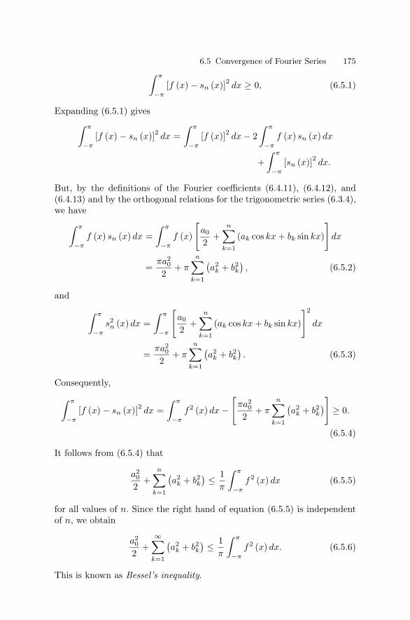
6.5 Convergence of Fourier Series 175∫ π
−π
[f (x) − sn (x)]2 dx ≥ 0, (6.5.1)
Expanding (6.5.1) gives∫ π
−π
[f (x) − sn (x)]2 dx =∫ π
−π
[f (x)]2 dx − 2∫ π
−π
f (x) sn (x) dx
+∫ π
−π
[sn (x)]2 dx.
But, by the definitions of the Fourier coefficients (6.4.11), (6.4.12), and(6.4.13) and by the orthogonal relations for the trigonometric series (6.3.4),we have∫ π
−π
f (x) sn (x) dx =∫ π
−π
f (x)
[a0
2+
n∑k=1
(ak cos kx + bk sin kx)
]dx
=πa2
0
2+ π
n∑k=1
(a2
k + b2k
), (6.5.2)
and ∫ π
−π
s2n (x) dx =
∫ π
−π
[a0
2+
n∑k=1
(ak cos kx + bk sin kx)
]2
dx
=πa2
0
2+ π
n∑k=1
(a2
k + b2k
). (6.5.3)
Consequently,∫ π
−π
[f (x) − sn (x)]2 dx =∫ π
−π
f2 (x) dx −[
πa20
2+ π
n∑k=1
(a2
k + b2k
)] ≥ 0.
(6.5.4)
It follows from (6.5.4) that
a20
2+
n∑k=1
(a2
k + b2k
) ≤ 1π
∫ π
−π
f2 (x) dx (6.5.5)
for all values of n. Since the right hand of equation (6.5.5) is independentof n, we obtain
a20
2+
∞∑k=1
(a2
k + b2k
) ≤ 1π
∫ π
−π
f2 (x) dx. (6.5.6)
This is known as Bessel’s inequality.

176 6 Fourier Series and Integrals with Applications
We see that the left side is nondecreasing and is bounded above, andtherefore, the series
a20
2+
∞∑k=1
(a2
k + b2k
), (6.5.7)
converges. Thus, the necessary condition for the convergence of series (6.5.7)is that
limk→∞
ak = 0, limk→∞
bk = 0. (6.5.8)
The Fourier series is said to converge in the mean to f (x) when
limn→∞
∫ π
−π
[f (x) −
(a0
2+
n∑k=1
ak cos kx + bk sin kx
)]2
dx = 0. (6.5.9)
If the Fourier series converges in the mean to f (x), then
a20
2+
∞∑k=1
(a2
k + b2k
)=
1π
∫ π
−π
f2 (x) dx. (6.5.10)
This is called Parseval’s relation and is one of the central results in thetheory of Fourier series. This relation is frequently used to derive the sumof many important numerical infinite series. Furthermore, if the relation(6.5.9) holds true, the set of trigonometric functions 1, cosx, sin x, cos 2x,sin 2x, . . . is said to be complete.
The Parseval relation (6.5.10) can formally be derived from the conver-gence of Fourier series to f (x) in [−π, π]. In other words, if
f (x) =12a0 +
∞∑k=1
(ak cos kx + bk sin kx) , (6.5.11)
where a0, ak and bk are given by (6.4.11), (6.4.12) and (6.4.13) respectively,we multiply ( 6.4.11) by 1
π f (x) and integrate the resulting expression from−π to π to obtain
1π
∫ π
k=1f2 (x) dx =
a0
2π
∫ π
−π
f (x) dx +∞∑
k=1
[ak
π
∫ π
−π
f (x) cos kx dx
+bk
π
∫ π
−π
f (x) sin kx dx
].(6.5.12)
Replacing all integrals on the right hand side of (6.5.12) by the Fouriercoefficients gives the Parseval relation (6.5.10).

6.6 Examples and Applications of Fourier Series 177
6.6 Examples and Applications of Fourier Series
The Fourier coefficients (6.4.11), (6.4.12), and (6.4.13) of Section 6.4 maybe obtained in a different way. Suppose the function f (x) of period 2π hasthe Fourier series expansion
f (x) =a0
2+
∞∑k=1
(ak cos kx + bk sin kx) . (6.6.1)
If we assume that the infinite series is term-by-term integrable (we willsee later that uniform convergence of the series is a sufficient condition forthis), then∫ π
−π
f (x) dx =∫ π
−π
[a0
2+
∞∑k=1
(ak cos kx + bk sin kx)
]dx = πa0.
Hence,
a0 =1π
∫ π
−π
f (x) dx. (6.6.2)
Again, we multiply both sides of equations (6.6.1) by cosnx and integratethe resulting expression from −π to π. We obtain∫ π
−π
f (x) cos nx dx =∫ π
−π
[a0
2+
∞∑k=1
(ak cos kx + bk sin kx)
]cos nx dx = πak.
Thus,
ak =1π
∫ π
−π
f (x) cos kx dx. (6.6.3)
In a similar manner, we find that
bk =1π
∫ π
−π
f (x) sin kx dx. (6.6.4)
The coefficients a0, ak, bk just found are exactly the same as those obtainedin Section 6.4.
Example 6.6.1. Find the Fourier series expansion for the function shown inFigure 6.6.1.
f (x) = x + x2, −π < x < π.
Here

178 6 Fourier Series and Integrals with Applications
Figure 6.6.1 Graph of f (x) = x + x2.
a0 =1π
∫ π
−π
f (x) dx =1π
∫ π
−π
(x + x2) dx =
2π2
3,
and
ak =1π
∫ π
−π
f (x) cos kx dx
=1π
∫ π
−π
(x + x2) cos kx dx
=1π
[x sin kx
k
∣∣∣∣π−π
−∫ π
−π
sin kx
kdx
]
+1π
[x2 sin kx
k
∣∣∣∣π−π
−∫ π
−π
2x sin kx
kdx
]
= − 2kπ
[−x cos kx
k
∣∣∣∣π−π
+∫ π
−π
cos kx
kdx
]
=4k2 cos kπ =
4k2 (−1)k for k = 1, 2, 3, . . . .
Similarly,

6.6 Examples and Applications of Fourier Series 179
bk =1π
∫ π
−π
f (x) sin kx dx
=1π
∫ π
−π
(x + x2) sin kx dx
= −2k
cos kπ = −2k
(−1)k, for k = 1, 2, 3, . . . .
Therefore, the Fourier series expansion for f is
f (x) =π2
3+
∞∑k=1
[4k2 (−1)k cos kx − 2
k(−1)k sin kx
]=
π2
3− 4 cos x + 2 sinx + cos 2x − sin 2x − . . . . (6.6.5)
Example 6.6.2. Consider the periodic function shown in Figure 6.6.2.
f (x) =
⎧⎨⎩−π, −π < x < 0,
x, 0 < x < π.
In this case,
a0 =1π
∫ π
−π
f (x) dx
=1π
[∫ 0
−π
−πdx +∫ π
0x dx
]= −π
2,
Figure 6.6.2 Graph of f (x).

180 6 Fourier Series and Integrals with Applications
and
ak =1π
∫ π
−π
f (x) cos kx dx
=1π
[∫ 0
−π
−π cos kx dx +∫ π
0x cos kx dx
]=
1k2π
(cos kπ − 1) =1
k2π
[(−1)k − 1
].
Also
bk =1π
∫ π
−π
f (x) sin kx dx
=1π
[∫ 0
−π
−π sin kx dx +∫ π
0x sin kx dx
]=
1k
(1 − 2 cos kπ) =1k
[1 − 2 (−1)k
].
Hence, the Fourier series is
f (x) = −π
4+
∞∑k=1
1
k2π
[(−1)k − 1
]cos kx +
1k
[1 − 2 (−1)k
]sin kx
.
(6.6.6)
Example 6.6.3. Consider the sawtooth wave function f (x) = x in the in-terval −π < x < π, f (x) = f (x+ 2kπ) for k = 1, 2, . . ..
This is a periodic function with period 2π and represents a sawtoothwave function as shown in Figure 6.6.3 and it is piecewise continuous.
Figure 6.6.3 The sawtooth wave function.

6.6 Examples and Applications of Fourier Series 181
We can readily find that
ak = 0, k = 0, 1, 2, . . . .
The coefficients bk are given by
bk =1π
∫ π
−π
f (x) sin kx dx
=1π
∫ π
−π
x sin kx dx =2k
(−1)k+1.
Hence, the Fourier series is
f (x) = 2∞∑
k=1
(−1)k+1 sin kx
k= 2
(sin x
1− sin 2x
2+
sin 3x3
− sin 4x4
+ . . .
).
(6.6.7)
This Fourier series does not agree with the function at every point in [−π, π].At the endpoints x = +π, the series is equal to zero, but the function doesnot vanish at either endpoint. However, the Fourier series (6.6.7) convergesto the value x at each point x in −π < x < π, but it converges to 0 =12 [f (π − 0) + f (π + 0)] = 1
2 (π − π) which is the mean value of the twolimits as x → + π. Thus, the convergence is not uniform. The partial sumof the series is
sn (x) = 2n∑
k=1
1k
(−1)k+1 sin kx. (6.6.8)
In the neighborhood of x = +π, the difference between f (x)and sn (x)seems not to become smaller as n increases, but the size of the region wherethis occurs decreases indicating nonuniform convergence. This nonuni-form oscillatory nature close to discontinuities is known as the Gibbs phe-nomenon.
It is important to point out that the sawtooth wave function f is notcontinuous in each point in [−π, π]. What happens in the neighborhood ofx = +π?
We consider the partial sum sn (x) given by (6.6.8), and put xn = π− πn
to approximate the value sn (x). We have
sn (xn) =n∑
k=1
2 (−1)k+1
ksin k
(π − π
n
)=
n∑k=1
2k
sin(
kπ
n
)which can be rewritten in the form
= 2n∑
k=1
sin(
πkn
)(πkn
) ·(π
n
). (6.6.9)

182 6 Fourier Series and Integrals with Applications
This sum can be identified with a Riemann sum of the definite integral
2∫ π
0
(sin x
x
)dx
which is obtained by dividing the interval [0, π] into the n subintervals[(k−1)π
n , kπn
], 1 ≤ k ≤ n. Obviously, each subinterval is of length
(πn
), and
we evaluate the function in each such subinterval at the right-hand endpointkπn , 1 ≤ k ≤ n. Consequently,
limn→∞ sn (x) = 2
∫ π
0
sin x
xdx ≈ 1.18π.
The point xn, as n → ∞, approaches x = π from the left. Hence, f (xn)tends to the value π. The jump at the point x = π is f (π−)−f (π+) = 2π,and, therefore, for sufficiently large n,
sn (xn) − f (xn)f (π−) − f (π+)
≈ 1.18π − π
2π= 0.09.
We next draw the graphs of s7 (x) and s10 (x) which exhibit oscillations overthe graph of f as shown in Figures 6.6.4 (a) and (b). These graphs showthe so-called overshooting in a neighborhood of x = +π and x = + 3π, andhence, the Gibbs phenomenon.
We next derive the sum of several numerical series from Example 6.6.3.Substituting x = π
2 in (6.6.7) gives
π
2= 2
∞∑k=1
(−1)k+1
ksin
(πk
2
)= 2
[1 − 1
3+
15
− 17
+ . . .
].
This gives the well-known slowly convergent numerical series
1 − 13
+15
− 17
+ . . . =π
4. (6.6.10)
On the other hand, putting x = π4 in (6.6.7) gives another numerical series
π
8=
1√2
− 12
+1
3√
2− 1
5√
2− 1
6− 1
7√
2+
19√
2− 1
10+
111
√2
− 113
√2
+114
− . . .
=1√2
(1 +
13
− 15
− 17
+19
+111
− . . .
)−1
2
(1 − 1
3+
15
− 17
+ . . .
)In view of (6.6.10), we obtain another numerical series
1 +13
− 15
− 17
+19
+111
− . . . =π
2√
2. (6.6.11)

6.7 Examples and Applications of Cosine and Sine Fourier Series 183
Figure 6.6.4 Graphs of s7 (x) in (a) and s10 (x) in (b).
6.7 Examples and Applications of Cosine and SineFourier Series
Let f (x) be an even function defined on the interval [−π, π]. Since cos kxis an even function, and sin kx an odd function, the function f (x) cos kx isan even function and the function f (x) sin kx an odd function. Thus, wefind that the Fourier coefficients of f (x) are
ak =1π
∫ π
−π
f (x) cos kx dx =2π
∫ π
0f (x) cos kx dx, k = 0, 1, 2, . . . ,
(6.7.1)
bk =1π
∫ π
−π
f (x) sin kx dx = 0, k = 1, 2, 3, . . . .

184 6 Fourier Series and Integrals with Applications
Hence, the Fourier series of an even function can be written as
f (x) ∼ a0
2+
∞∑k=1
ak cos kx, (6.7.2)
where the coefficients ak are given by formula (6.7.1).In a similar manner, if f (x) is an odd function, the function f (x) cos kx
is an odd function and the function f (x) sin kx is an even function. As aconsequence, the Fourier coefficients of f (x), in this case, are
ak =1π
∫ π
−π
f (x) cos kx dx = 0, k = 0, 1, 2, . . . , (6.7.3)
bk =1π
∫ π
−π
f (x) sin kx dx =2π
∫ π
0f (x) sin kx dx, k = 1, 2, . . . . (6.7.4)
Therefore, the Fourier series of an odd function can be written as
f (x) =∞∑
k=1
bk sin kx, (6.7.5)
where the coefficients bk are given by formula (6.7.4).
Example 6.7.1. Obtain the Fourier series of the function
f (x) = sgn x =
⎧⎨⎩−1, −π < x < 0,0, x = 0,
+1, 0 < x < π,and f (x+ 2kπ) = f (x) .
In this case, f is an odd function with period 2π and represents squarewave function as shown in Figure 6.7.1. Clearly, ak = 0 for k = 0, 1, 2, 3, . . .and
bk =2π
∫ π
0f (x) sin kx dx
=2π
∫ π
0sin kx dx =
2kπ
[1 − (−1)k
].
Thus, b2k = 0 and b2k−1 = [(4/π) (2k − 1)]. Therefore, the Fourier series ofthe function f (x) is
f (x) =4π
∞∑k=1
sin (2k − 1) x
(2k − 1). (6.7.6)
This Fourier series consists of only odd harmonics. The loss of evenharmonics is due to the fact that sgn
( 12 + x
)= sgn
( 12 − x
).
Putting x = π4 in (6.7.6) gives (6.6.10).
The nth partial sum of the series (6.7.6) is

6.7 Examples and Applications of Cosine and Sine Fourier Series 185
Figure 6.7.1 The square wave function.
sn (x) =4π
n∑k=1
sin (2k − 1) x
(2k − 1). (6.7.7)
We now examine the manner in which the first n terms of the series (6.7.7)tend to f (x) as n → ∞. The graphs of sn (x) for n = 1, 3, 5 is shown inFigure 6.7.2. To investigate the oscillations as n → ∞, we locate the firstpeak to the right of the origin and calculate its height as n → ∞.
Figure 6.7.2 The Gibbs phenomenon.

186 6 Fourier Series and Integrals with Applications
The peak overshoot occurs at a local maximum of the partial sum sn (x)so that
0 = s′n (x) =
4π
n∑k=1
cos (2k − 1) x
=2
π sin x
n∑k=1
2 sin x cos (2k − 1) x
=2
π sin x
n∑k=1
[sin 2kx − sin (2k − 2) x]
=2 sin nx
π sin x. (6.7.8)
This leads to the points of maximum at x = π2n , 2π
2n , . . . , (2n − 1) π2n so
that the first peak to the right of the origin occurs at x = π2n . So, the value
of sn (x) at this point is
sn
( π
2n
)=
2π
· π
n
n∑k=1
sin (2k − 1) π2n
(2k − 1) π2n
.
In the limit as n → ∞, this becomes
limn→∞ sn
( π
2n
)=
(2π
)lim
n→∞π
n
n∑k=1
sin (2k − 1) π2n
(2k − 1) π2n
=2π
∫ π
0
sin x
xdx =
2π
(1.852) = 1.179.
Instead of a maximum value 1, it turns out to be 1.179 approximately.If the overshoot is compared to the jump in the function it is about12 (1.179 − 1) × 100% ∼ 9%. The onset of the Gibbs phenomenon is shownin the Figure 6.7.3.
Historically, this phenomenon was first observed by a physicist A.Michelson (1852–1931) at the end of the nineteenth century. In order tocalculate some Fourier coefficients of a function graphically, he developedequipment that is called a harmonic analyser and synthesizer. He calcu-lated some partial sums, sn, of a given function f graphically. Michelsonalso observed from this graphical representation that, for some functions,the graphs of sn were very close to the function. However, for the sgnfunction, the graphs of the partial sums exhibit a large error in the neigh-borhood of the origin, x = 0 and x = +π (the jump discontinuities ofthe function) independent of the number of terms in the partial sums. Itwas J.W. Gibbs (1839–1903) who first provided the explanation for thisstrikingly new phenomenon and showed that these large errors were not as-sociated with numerical computations. Indeed, he further showed that the

6.7 Examples and Applications of Cosine and Sine Fourier Series 187
Figure 6.7.3 The Gibbs phenomenon.
large errors occur at every jump discontinuity for every piecewise continu-ous function f in [−π, π] with certain derivative properties near the jumpdiscontinuity.
Example 6.7.2. Expand |sin x| in Fourier series. Since |sin x| is an even func-tion, as shown in Figure 6.7.4, bk = 0 for k = 1, 2, . . . and
ak =2π
∫ π
0f (x) cos kx dx
=2π
∫ π
0sin x cos kx dx
=1π
∫ π
0[sin (1 + k) x + sin (1 − k) x] dx
=2[1 + (−1)k
]π (1 − k2)
for k = 0, 2, 3, . . . .
For k = 1,
a1 =2π
∫ π
0sin x cos x dx = 0.
Hence, the Fourier series of f (x) is
f (x) =2π
+4π
∞∑k=1
cos (2kx)(1 − 4k2)
.
Example 6.7.3. Find the Fourier series of the triangular wave function whichis defined by

188 6 Fourier Series and Integrals with Applications
Figure 6.7.4 The rectified sine function.
f (x) = |x| =
⎧⎨⎩−x, −π ≤ x ≤ 0
x, 0 ≤ x ≤ π(6.7.9)
and f (x) = f (x+ 2nπ), n = 1, 2, 3, . . ..
This is an even periodic function with period 2π as shown in Figure 6.7.5.
This function gives a Fourier cosine series with bn = 0 for all n and
Figure 6.7.5 Triangular wave function.

6.7 Examples and Applications of Cosine and Sine Fourier Series 189
a0 =1π
∫ π
−π
|x| dx =2π
∫ π
0x dx = π
an =1π
∫ π
−π
|x| cos nx dx =2π
∫ π
0|x| cos nx dx
=2π
∫ π
0x cos nx dx =
2π
([x sin nx
n
]π
0−
∫ π
0
sin nx
ndx
),
integrating by parts
=2
πn2 [cos nx]π0 =2
πn2 [(−1)n − 1] =
⎧⎨⎩0, if n is even,
− 4πn2 if n is odd.
Thus, the Fourier cosine series is given by
f (x) =12a0 +
∞∑n=1
an cos nx
=π
2− 4
π
(cos x
12 +cos 3x
32 +cos 5x
52 + . . .
). (6.7.10)
Substituting x = 0 in (6.7.10) yields the following numerical series
π2
8=
112 +
132 +
172 + . . . =
∞∑n=1
1(2n − 1)2
. (6.7.11)
This series can be used to derive the sum of reciprocals of squares of allpositive integers,
S =∞∑
n=1
1n2 =
π2
6(6.7.12)
and vise versa.We have
π2
8=
∞∑n=1
1(2n − 1)2
=∞∑
n=1
1n2 −
∞∑n=1
1(2n)2
= S − 14
∞∑n=1
1n2 = S − 1
4S.
This gives (6.7.12).The series (6.7.12) is just the value of s = 2 of the Riemann zeta function
defined by
ζ (s) =∞∑
n=1
1ns
, (6.7.13)

190 6 Fourier Series and Integrals with Applications
where s may be complex. This definition of ζ (s) can be extended in a nat-ural way and this extension is called the analytic continuation of ζ (s) toinclude all complex numbers s except for s = 1. This function was intro-duced by Bernhard Riemann in 1841. He proved many properties of thisfunction and made several conjectures, some of which are still open prob-lems in mathematics. It is well known that ζ (s) has zeros on the real axisonly at the even negative integers. Riemann conjectured that all complexzeros of ζ (s) lie on the line Re (s) = 1
2 . This is called the Riemann Hypoth-esis; it is still an unsolved problem in mathematics. However, it is provedthat there are an infinite number of zeros on the line. Indeed, by the fall of2002, fifty billion complex zeros have been found — all of them lie on thestated line.
Example 6.7.4. Obtain the Fourier series of f (x) = x2, −π ≤ x ≤ π, withf (x) = f (x+ 2nπ), for n = 1, 2, . . ..
Obviously, this is an even function, and its periodic extensions are shownin Figure 6.7.6.
Since f (x) is an even function, bn ≡ 0 for all n ≥ 1. It turns out that
Figure 6.7.6 Periodic extension of x2.

6.7 Examples and Applications of Cosine and Sine Fourier Series 191
a0 =1π
∫ π
−π
x2dx =2π
∫ π
0x dx =
2π2
3,
an =1π
∫ π
−π
x2 cos nx dx =2π
∫ π
0x2 cos nx dx
=2π
([x2
nsin nx
]π
0− 2
π
∫ π
0x sin nx dx
),
= − 4nπ
∫ x
0x sin nx dx
= − 4nπ
([−x
ncos nx
]π
0+
1π
∫ π
0cos nx dx
),
= − 4nπ
(−π
n(−1)n − 1
n2 [sinnx]π0
)=
4n2 (−1)n
, n ≥ 1.
Consequently, the Fourier cosine series for x2 is given by
x2 =π2
3+ 4
∞∑n=1
1n2 (−1)n cos nx
=π2
3− 4
(cos x
12 − cos 2x
22 +cos 3x
32 − . . .
). (6.7.14)
Putting x = 0 in (6.7.14) gives the following numerical series
112 − 1
22 +132 − 1
42 + · · · =π2
12. (6.7.15)
Substituting x = π in (6.7.14) yields (6.7.12) which can also be obtainedfrom (6.7.15) and vice versa. Thus, we have
S =∞∑
n=1
1n2 =
112 +
122 +
132 +
142 +
152 +
162 + · · ·
=(
111 − 1
22 +132 − 1
42 + · · ·)
+ 2(
122 +
142 +
162 + · · ·
)=
π2
12+
24
(112 +
122 +
132 + · · ·
)=
π2
12+
12S,
which gives the value of S = π2
6 . Adding (6.7.12) and (6.7.15) gives
112 +
132 +
152 + · · · =
π2
8, (6.7.16)
and then, subtracting (6.7.15) from (6.7.12) yields
122 +
142 +
162 +
182 + · · · =
π2
24. (6.7.17)

192 6 Fourier Series and Integrals with Applications
Figure 6.7.7 Periodic extension of f (x).
In the preceding sections, we have prescribed the function f (x) in theinterval (−π, π) and assumed f (x) to be periodic with period 2π in theentire interval (−∞,∞). In practice, we frequently encounter problems inwhich a function is defined only in the interval (−π, π). In such a case, wesimply extend the function periodically with period 2π, as in Figure 6.7.7.In this way, we are able to represent the function f (x) by the Fourier seriesexpansion, although we are interested only in the expansion on (−π, π).
If the function f is defined only in the interval (0, π), we may extend fin two ways. The first is the even extension of f , denoted and defined by(see Figure 6.7.8)
Fe (x) =
⎧⎨⎩f (x) , 0 < x < π,
f (−x) , −π < x < 0,
while the second is the odd extension of f , denoted and defined by (seeFigure 6.7.9)
F0 (x) =
⎧⎨⎩f (x) , 0 < x < π,
−f (−x) , −π < x < 0.

6.7 Examples and Applications of Cosine and Sine Fourier Series 193
Figure 6.7.8 Even extension of f (x).
Since Fe (x) and F0 (x) are even and odd functions with period 2π respec-tively, the Fourier series expansions of Fe (x) and F0 (x) are
Fe (x) =a0
2+
∞∑k=1
ak cos kx,
where
ak =2π
∫ π
0f (x) cos kx dx,
and
Figure 6.7.9 Odd extension of f (x).

194 6 Fourier Series and Integrals with Applications
F0 (x) =∞∑
k=1
bk sin kx,
where
bk =2π
∫ π
0f (x) sin kx dx.
6.8 Complex Fourier Series
It is sometimes convenient to represent a function by an expansion in com-plex form. This expansion can easily be derived from the Fourier series
f (x) =a0
2+
∞∑k=1
(ak cos kx + bk sin kx) .
Using Euler’s formulas
cos x =eix + e−ix
2, sin x =
eix − e−ix
2i,
we write
f (x) =a0
2+
∞∑k=1
[ak
(eikx + e−ikx
2
)+ bk
(eikx − e−ikx
2i
)]
=a0
2+
∞∑k=1
[(ak − ibk
2
)eikx +
(ak + ibk
2
)e−ikx
]
= c0 +∞∑
k=1
(ck eikx + c−k e−ikx
),
where
c0 =a0
2=
12π
∫ π
−π
f (x) dx
ck =ak − ibk
2=
12π
∫ π
−π
f (x) (cos kx − i sin kx) dx
=12π
∫ π
−π
f (x) e−ikxdx
c−k =ak + ibk
2=
12π
∫ π
−π
f (x) (cos kx + i sin kx) dx
=12π
∫ π
−π
f (x) eikxdx.
Thus, we obtain the Fourier series expansion for f (x) in complex form

6.8 Complex Fourier Series 195
f (x) =∞∑
k=−∞ck eikx, −π < x < π, (6.8.1)
where
ck =12π
∫ π
−π
f (x) e−ikxdx. (6.8.2)
We derive the following Parseval formula
12π
∫ π
−π
f2 (x) dx =∞∑
k=−∞|ck|2 . (6.8.3)
from formulas (6.8.1)–(6.8.2).Multiplying (6.8.1) by 1
2π f (x) and integrating from −π < x < π yields
12π
∫ π
−π
f2 (x) dx =∞∑
k=−∞ck · 1
2π
∫ π
−π
f (x) eikxdx
=∞∑
k=−∞ck · c−k =
∞∑k=−∞
ck ck =∞∑
k=−∞|ck|2 .
Example 6.8.1. Obtain the complex Fourier series expansion for the func-tion
f (x) = ex, −π < x < π.
We find
ck =12π
∫ π
−π
f (x) e−ikxdx
=12π
∫ π
−π
exe−ikxdx
=(1 + ik) (−1)k
π (1 + k2)sinhπ,
and hence, the Fourier series is
f (x) =∞∑
k=−∞
(1 + ik) (−1)k
π (1 + k2)sinhπ eikx. (6.8.4)
We apply the Parseval formula (6.8.3) to this example and obtain∞∑
k=−∞
|1 + ik|2 sinh2 π
π2 (1 + k2)2=
14π
(e2π − e−2π
)=
12π
sinh 2π.
Simplifying this result gives∞∑
k=−∞
1(1 + k2)
= π coth π. (6.8.5)

196 6 Fourier Series and Integrals with Applications
Example 6.8.2. Show that, for −1 < a < 1,
∞∑n=0
an cos nx =1 − a cos x
1 − 2a cos x + a2 , (6.8.6)
∞∑n=0
an sin nx =a sin x
1 − 2a cos x + a2 . (6.8.7)
We denote the cosine series by C and sine series by S so that
C + iS =∞∑
n=0
an (cos nx + i sin nx) =∞∑
n=0
(a eix
)n
=1
1 − a eix, since
∣∣a eix∣∣ < 1.
=1
1 − a cos x − ia sin x=
(1 − a cos x) + ia sin x
(1 − a cos x)2 + a2 sin2 x
=(1 − a cos x) + ia sin x
1 − 2a cos x + a2 . (6.8.8)
Equating the real and imaginary part gives the desired results.
6.9 Fourier Series on an Arbitrary Interval
So far we have been concerned with functions defined on the interval [−π, π].In many applications, however, this interval is restrictive, and the intervalof interest may be arbitrary, say [a, b].
If we introduce the new variable t by the transformation
x =12
(b + a) +(b − a)
2πt, (6.9.1)
then, the interval a ≤ x ≤ b becomes −π ≤ t ≤ π. Thus, the functionf [(b + a) /2 + ((b − a) /2π) t] = F (t) obviously has period 2π. Expandingthis function in a Fourier series, we obtain
F (t) =a0
2+
∞∑k=1
(ak cos kt + bk sin kt) , (6.9.2)
where
ak =1π
∫ π
−π
F (t) cos kt dt, k = 0, 1, 2, . . . ,
and
bk =1π
∫ π
−π
F (t) sin kt dt, k = 1, 2, 3, . . . .

6.9 Fourier Series on an Arbitrary Interval 197
On changing t into x, we find the expansion for f (x) in [a, b]
f (x) =a0
2+
∞∑k=1
[ak cos
kπ (2x − b − a)(b − a)
+ bk sinkπ (2x − b − a)
(b − a)
],(6.9.3)
where
ak =2
b − a
∫ b
a
f (x) cos[kx (2x − b − a)
(b − a)
]dx, k = 0, 1, 2, . . . , (6.9.4)
bk =2
b − a
∫ b
a
f (x) sin[kx (2x − b − a)
(b − a)
]dx, k = 1, 2, 3, . . . . (6.9.5)
It is sometimes convenient to take the interval in which the function f isdefined as [−l, l]. It follows at once from the result just obtained that byletting a = −l and b = l, the Fourier expansion for f in [−l, l] takes theform
f (x) =a0
2+
∞∑k=1
[ak cos
(kπx
l
)+ bk sin
(kπx
l
)], (6.9.6)
where
ak =1l
∫ l
−l
f (x) cos(
kπx
l
)dx, k = 0, 1, 2, . . . , (6.9.7)
bk =1l
∫ l
−l
f (x) sinkπx
ldx, k = 1, 2, 3, . . . . (6.9.8)
If f is an even function of period 2l, then, from equation (6.9.6), we canreadily determine the Fourier cosine expansion in the form
f (x) =a0
2+
∞∑k=1
ak cos(
kπx
l
), (6.9.9)
where
ak =2l
∫ l
0f (x) cos
(kπx
l
)dx, k = 0, 1, 2, . . . . (6.9.10)
If f is an odd function of period 2l, then, from equation (6.9.6), the Fouriersine expansion for f is
f (x) =∞∑
k=1
bk sin(
kπx
l
), (6.9.11)
where

198 6 Fourier Series and Integrals with Applications
bk =2l
∫ l
0f (x) cos
(kπx
l
)dx. (6.9.12)
Finally, we make a change of variable to obtain the complex Fourier seriesof f (x) on the interval −l < x < l. Suppose f (x) is a periodic functionwith period 2l. We put a = −l and b = l so that the change of variableformula becomes x = lt
π and
f (x) = f
(lt
π
)= F (t) . (6.9.13)
Clearly, F (t) is periodic with period 2π. If it is piecewise smooth, it can beexpanded in a complex Fourier series in the form
F (t) =∞∑
k=−∞ckeikt, ck =
12π
∫ π
−π
F (t) e−iktdt. (6.9.14)
Substituting t = πxl into (6.9.14) gives the complex Fourier series expansion
of the original function f in the form
f (x) =∞∑
k=−∞ck exp
(ixπk
l
), ck =
12l
∫ l
−l
f (x) exp(
− ixπk
l
)dx.(6.9.15)
In particular, if f (t) is a periodic function of time variable t with periodT = 2π
ω and ω(= 2π
T = πl
)is the frequency, then
f (t) =a0
2+
∞∑n=1
[an cos (nωt) + bn sin (nωt)] , (6.9.16)
where anand bn are given by (6.9.7) and (6.9.8) with πl replaced by ω and
k = n. The terms (a1 cos ωt + b1 sin ωt), (a2 cos 2ωt + b2 sin 2ωt), . . .,(an cos nωt + bn sin nωt), . . . are called the first, the second, and the nthharmonic respectively.
Example 6.9.1. Consider the odd periodic function
f (x) = x, −2 < x < 2,
as shown in Figure 6.9.1. Here l = 2. Since f is odd, ak = 0, and
bk =2l
∫ l
0f (x) sin
(kπx
l
)dx,
=22
∫ 2
0x sin
(kπx
2
)dx = − 4
kπ(−1)k for k = 1, 2, 3, . . . .
Therefore, the Fourier sine series of f is
f (x) =∞∑
k=1
4kπ
(−1)k+1 sin(
kπx
2
).

6.9 Fourier Series on an Arbitrary Interval 199
Figure 6.9.1 Odd periodic function of f (x) = x in −2 < x < 2.
Example 6.9.2. Consider the function
f (x) =
⎧⎨⎩1, 0 < x < 1
2
0, 12 < x < 1.
In this case, the period is 2l = 2 or l = 1. Extend f as shown in Figure6.9.2. Since the extension is even, we have bk = 0 and
a0 =2l
∫ l
0f (x) dx =
21
∫ 12
0dx = 1
ak =2l
∫ l
0f (x) cos
(kπx
l
)dx
=21
∫ 1
0cos (kπx) dx =
(2kπ
)sin
(kπ
2
).
Hence,
f (x) =12
+∞∑
k=1
2(2k − 1) π
(−1)k−1 cos (2k − 1) πx.
Example 6.9.3. Find the Fourier series of f (x) = x2 in (−l, l) from thecorresponding Fourier series in (−π, π).

200 6 Fourier Series and Integrals with Applications
Figure 6.9.2 Even extension of f (x) in Example 6.9.2.
It directly follows from (6.7.14) and (6.9.9) as
f (x) = x2 =π2
3+ 4
∞∑k=1
1k2 (−1)k cos
(πkx
l
), −l < x < l.
Example 6.9.4. Find the sine and cosine Fourier series of f (x) = x in (0, l)from the corresponding Fourier series in (0, π).
We know the Fourier sine series for x in (0, π)
f (x) = x = 2∞∑
k=1
(−1)k+1
ksin kx, 0 < x < π.
Using the transformation x =(
πtl
), we obtain
t =2l
π
∞∑k=1
(−1)k+1
ksin
(πkt
l
), 0 < x < l.
We have the Fourier cosine series for x in (0, π)
f (x) = x =π
2− 4
π
∞∑k=1
1(2k − 1)2
cos (2k − 1) x, 0 < x < π.
Similarly, using the transformation x = πtl gives
t =l
2− 4l
π2
∞∑k=1
1(2k − 1)2
cos[(2k − 1)
πt
l
], 0 < x < l.
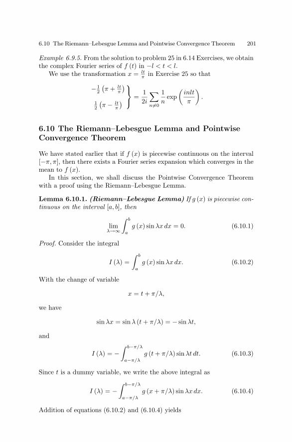
6.10 The Riemann–Lebesgue Lemma and Pointwise Convergence Theorem 201
Example 6.9.5. From the solution to problem 25 in 6.14 Exercises, we obtainthe complex Fourier series of f (t) in −l < t < l.
We use the transformation x = ltπ in Exercise 25 so that
− 12
(π + lt
π
)12
(π − lt
π
)⎫⎬⎭ =
12i
∑n =0
1n
exp(
inlt
π
).
6.10 The Riemann–Lebesgue Lemma and PointwiseConvergence Theorem
We have stated earlier that if f (x) is piecewise continuous on the interval[−π, π], then there exists a Fourier series expansion which converges in themean to f (x).
In this section, we shall discuss the Pointwise Convergence Theoremwith a proof using the Riemann–Lebesgue Lemma.
Lemma 6.10.1. (Riemann–Lebesgue Lemma) If g (x) is piecewise con-tinuous on the interval [a, b], then
limλ→∞
∫ b
a
g (x) sinλx dx = 0. (6.10.1)
Proof. Consider the integral
I (λ) =∫ b
a
g (x) sinλx dx. (6.10.2)
With the change of variable
x = t + π/λ,
we have
sin λx = sinλ (t + π/λ) = − sin λt,
and
I (λ) = −∫ b−π/λ
a−π/λ
g (t + π/λ) sinλt dt. (6.10.3)
Since t is a dummy variable, we write the above integral as
I (λ) = −∫ b−π/λ
a−π/λ
g (x + π/λ) sinλx dx. (6.10.4)
Addition of equations (6.10.2) and (6.10.4) yields

202 6 Fourier Series and Integrals with Applications
2I (λ) =∫ b
a
g (x) sinλx dx −∫ b−π/λ
a−π/λ
g (x + π/λ) sinλx dx
= −∫ a
a−π/λ
g (x + π/λ) sinλx dx +∫ b
b−π/λ
g (x) sinλx dx
+∫ b−π/λ
a
[g (x) − g (x + π/λ)] sinλx dx. (6.10.5)
First, let g (x) be a continuous function in [a, b]. Then g (x) is necessarilybounded, that is, there exists an M such that |g (x)| ≤ M . Hence,∣∣∣∣∣
∫ a
a−π/λ
g (x + π/λ) sinλx dx
∣∣∣∣∣ =
∣∣∣∣∣∫ a+π/λ
a
g (x) sinλx dx
∣∣∣∣∣ ≤ πM
λ,
and ∣∣∣∣∣∫ b
b−π/λ
g (x) sinλx dx
∣∣∣∣∣ ≤ πM
λ.
Consequently,
|I (λ)| ≤ πM
λ+
∫ b−π/λ
a
|g (x) − g (x + π/λ)| dx. (6.10.6)
Since g (x) is a continuous function on a closed interval [a, b], it is uniformlycontinuous on [a, b] so that
|g (x) − g (x + π/λ)| < ε/ (b − a) , (6.10.7)
for all λ > Λ and all x in [a, b]. We now choose λ such that πM/λ < ε/2,whenever λ > Λ. Then
|I (λ)| <ε
2+
ε
2= ε.
If g (x) is piecewise continuous in [a, b], then the proof consists of arepeated application of the preceding argument to every subinterval of [a, b]in which g (x) is continuous.
Theorem 6.10.1. (Pointwise Convergence Theorem). If f (x) is piece-wise smooth and periodic function with period 2π in [−π, π], then for anyx
a0
2+
∞∑k=1
(ak cos kx + bk sin kx) =12
[f (x+) + f (x−)] , (6.10.8)
where
ak =1π
∫ π
−π
f (t) cos kt dt, k = 0, 1, 2, . . . , (6.10.9)
bk =1π
∫ π
−π
f (t) sin kt dt, k = 1, 2, 3, . . . . (6.10.10)

6.10 The Riemann–Lebesgue Lemma and Pointwise Convergence Theorem 203
Proof. The nth partial sum sn (x) of the series (6.10.8) is
sn (x) =12a0 +
n∑k=1
(ak cos kx + bk sin kx) . (6.10.11)
We use integrals in (6.10.9)–(6.10.10) to replace ak and bk in (6.10.11)so that
sn (x) =12π
∫ π
−π
[1 + 2
n∑k=1
(cos kt cos kx + sin kt sin kx)
]f (t) dt
=12π
∫ π
−π
[1 + 2
n∑k=1
cos k (x − t)
]f (t) dt
=12π
∫ π
−π
Dn (x − t) f (t) dt, (6.10.12)
where Dn (θ) is called the Dirichlet kernel defined by
Dn (θ) = 1 + 2n∑
k=1
cos kθ. (6.10.13)
The next step is to study the properties of this kernel Dn (θ) which isan even function with period 2π and satisfies the condition
12π
∫ π
−π
Dn (θ) dθ = 1 + 0 + 0 + . . . + 0 = 1. (6.10.14)
We find the value of the sum in (6.10.13) by Euler’s formula so that
Dn (θ) = 1 +n∑
k=1
(eikθ + e−ikθ
)=
n∑k=−n
eikθ
= e−inθ + . . . + 1 + . . . + einθ.
This is a finite geometric series with the first term e−inθ, the ratio eiθ, andthe last term einθ, and hence, its sum is given by
Dn (θ) =e−inθ − ei(n+1)θ
1 − eiθ
=exp
[− (n + 1
2
)iθ
] − exp[(
n + 12
)iθ
]exp
(− 12 iθ
) − exp(+ 1
2 iθ)
=sin
(n + 1
2
)θ
sin 12θ
. (6.10.15)
The graph of Dn (θ) is shown in Figure 6.10.1. It looks similar to that ofthe diffusion kernel as drawn in Figure 12.4.1 in Chapter 12 except for itssymmetric oscillatory trail.

204 6 Fourier Series and Integrals with Applications
Figure 6.10.1 Graph of Dn (θ) against θ.
We next put t − x = θ in (6.10.12) to obtain
sn (x) =12π
∫ x+π
x−π
Dn (θ) f (x + θ) dθ. (6.10.16)
Since both Dn and f have period 2π, the limits of the integral can be takenfrom −π to π, and hence, (6.10.16) assumes the form
sn (x) =12π
∫ π
−π
Dn (θ) f (x + θ) dθ. (6.10.17)
We next use (6.10.14) to express the difference of sn (x) and 12 [f (x+) + f (x−)]
in the form
sn (x) − 12
[f (x+) + f (x−)]
=12π
∫ 0
−π
Dn (θ) [f (x + θ) − f (x−)] dθ
+12π
∫ π
0Dn (θ) [f (x + θ) − f (x+)] dθ
which is, by (6.10.15),
=12π
∫ 0
−π
g− (θ) sin(
n +12
)θ dθ +
12π
∫ π
0g+ (θ) sin
(n +
12
)θ dθ,
(6.10.18)

6.10 The Riemann–Lebesgue Lemma and Pointwise Convergence Theorem 205
where
g+ (θ) =(
sinθ
2
)−1
[f (x + θ) − f (x+ )] . (6.10.19)
Since the denominators of the functions g+ (θ) vanish at θ = 0, inte-grals in (6.10.18) may diverge at this point. However, by assumption, f ispiecewise smooth, and hence,
limθ→0 +
g+ (θ) = limθ→0 +
f (x + θ) − f (x)θ2
·(
θ2
sin θ2
)= 2f ′ (x+) .(6.10.20)
Evidently, the above limits exist, and g+ (θ) are piecewise continuous else-where in the interval (−π, π). Therefore, by the Riemann–Lebesgue Lemma6.10.1, both integrals in (6.10.18) vanish as n → ∞. Thus,
limn→∞ sn (x) =
12
[f (x+) + f (x−)] .
This proves that the Fourier series converges for each x in (−π, π).
Remark 3. At a point of continuity the series converges to the functionf (x).
Remark 4. At a point of discontinuity, the series is equal to the arithmeticmean of the limits of the function on both sides of the discontinuity.
Remark 5. The condition of piecewise smoothness under which the Fourierseries converges pointwise is a sufficient condition. A large number of ex-amples of applications is covered by this case. However, the pointwise con-vergence Theorem 6.10.1 can be proved under weaker conditions.
Example 6.10.1. In Example 6.6.1, we obtained that the Fourier series ex-pansion for
(x + x2
)in [−π, π], as shown in Figure 6.10.2, is
f (x) ∼ π2
3+
∞∑k=1
[4k2 (−1)k cos kx − 2
k(−1)k sin kx
].
Since f (x) = x + x2 is piecewise smooth, the series converges, and hence,we write
x + x2 =π2
3+
∞∑k=1
[4k2 (−1)k cos kx − 2
k(−1)k sin kx
],
at points of continuity. At points of discontinuity, such as x = π, by virtueof the Pointwise Convergence Theorem,

206 6 Fourier Series and Integrals with Applications
Figure 6.10.2 Graph of f (x).
12[(
π + π2) +(−π + π2)] =
π2
3+
∞∑k=1
4k2 (−1)k cos kπ, (6.10.21)
since
f (π−) = π + π2 and f (π+) = f (−π+) = −π + π2.
Simplification of equation (6.10.21) gives
π2 =π2
3+
∞∑k=1
4k2 (−1)2k
,
or
π2
6=
∞∑k=1
1k2 .
The series can be used to obtain the sum of reciprocals of squares of oddpositive integers, that is,
∞∑n=1
1(2n − 1)2
.
We have
π2
6=
∞∑n=1
1n2 =
∞∑n=1
1(2n)2
+∞∑
n=1
1(2n − 1)2
=14
· π2
6+
∞∑n=1
1(2n − 1)2
,

6.10 The Riemann–Lebesgue Lemma and Pointwise Convergence Theorem 207
or,
∞∑n=1
1(2n − 1)2
=π2
6
(1 − 1
4
)=
π2
8.
Conversely, this series can be used to find the sum of reciprocals of squaresof all positive integers.
Example 6.10.2. Find the Fourier series of the following function
f (x) =
⎧⎨⎩0, −2 ≤ x < 0
2 − x, 0 < x ≤ 2.
This function is defined over the interval −2 ≤ x ≤ 2, where it is piecewisesmooth with a finite discontinuity at x = 0. We use (6.9.7) and (6.9.8) tocalculate the Fourier coefficients
a0 =12
∫ 2
0(2 − x) dx = 1
ak =12
∫ 2
0(2 − x) cos
(πkx
2
)dx =
2π2k2
[1 − (−1)k
], k = 1, 2, 3, . . . .
bk =12
∫ 2
0(2 − x) sin
(πkx
2
)dx =
2πk
, k = 1, 2, 3, . . . .
Consequently, the Fourier series (6.9.6) becomes
f (x) =12
+2π
∞∑k=1
⎡⎣
1 − (−1)k
πk2 cos(
πkx
2
)+
1k
sin(
πkx
2
)⎤⎦ . (6.10.22)
The function f (x) is continuous at x = 1 where f (1) = 1, so that theFourier series (6.10.22) gives
1 =12
+2π
∞∑n=1
[1 − (−1)nπn2 cos
(nπ
2
)+
1n
sin(nπ
2
)].
Since the factor 1 − (−1)n = 0 for even n, and cos nπ2 = 0 when n is
odd, every term of the cosine series vanishes for all n. Consequently,
π
4=
∞∑n=1
1n
sin(nπ
2
)=
∞∑n=1
(−1)n
(2n + 1). (6.10.23)
On the other hand, f (x) is discontinuous at x = 0 and the Fourier seriesmust converge to 1
2 (0 + 2) = 1. Thus,

208 6 Fourier Series and Integrals with Applications
π2
4=
∞∑n=1
[1 − (−1)n]n2 = 2
∞∑n=1
1(2n − 1)2
,
or∞∑
n=1
1(2n − 1)2
=π2
8. (6.10.24)
6.11 Uniform Convergence, Differentiation, andIntegration
In the preceding section, we have proved the pointwise convergence of theFourier series for a piecewise smooth function. Here, we shall consider sev-eral theorems without proof concerning uniform convergence, term-by-termdifferentiation, and integration of Fourier series.
Theorem 6.11.1. (Uniform and Absolute Convergence Theorem)Let f (x) be a continuous function with period 2π, and let f ′ (x) be piecewisecontinuous in the interval [−π, π]. If, in addition, f (−π) = f (π), then theFourier series expansion for f (x) is uniformly and absolutely convergent.
In the preceding theorem, we have assumed that f (x) is continuousand f ′ (x) is piecewise continuous. With less stringent conditions on f , thefollowing theorem can be proved.
Theorem 6.11.2. Let f (x) be piecewise smooth in the interval [−π, π]. Iff (x) is periodic with period 2π, then the Fourier series for f convergesuniformly to f in every closed interval containing no discontinuity.
We note that the partial sums sn (x) of a Fourier series cannot approachthe function f (x) uniformly over any interval containing a point of discon-tinuity of f . The behavior of the deviation of sn (x) from f (x) in such aninterval is known as the Gibbs phenomenon. For instance, in the Example6.7.1, the Fourier series of the function is given by
f (x) =4π
∞∑k=1
sin (2k − 1) x
(2k − 1). (6.11.1)
From graphs of the partial sums sn (x) against the x-axis, as shown inFigures 6.7.2 and 6.7.3, we find that sn (x) oscillate above and below thevalue of f . It can be observed that, near the discontinuous points x = 0and x = π, sn deviate from the function rather significantly. Althoughthe magnitude of oscillation decreases at all points in the interval for largen, very near the points of discontinuity the amplitude remains practicallyindependent of n as n increases. This illustrates the fact that the Fourier

6.11 Uniform Convergence, Differentiation, and Integration 209
series of a function f does not converge uniformly on any interval whichcontains a discontinuity.
Termwise differentiation of Fourier series is, in general, not permissible.From Example 6.6.3, the Fourier series for f (x) = x is given by
x = 2[sin x − sin 2x
2+
sin 3x3
− . . .
], (6.11.2)
which converges for all x, whereas the series after formal term-by-termdifferentiation,
1 ∼ 2 [cos x − cos 2x + cos 3x − . . .] .
This series is not the Fourier series of f ′ (x) = 1, since the Fourier series off ′ (x) = 1 is the function 1. In fact, this series is not a Fourier series of anypiecewise continuous function defined in [−π, π] as the coefficients do nottend to zero which contradicts the Riemann–Lebesque lemma.
In fact, the series of f ′ (x) = 1 diverges for all x since the nth term,cos nx does not tend to zero as n → ∞. The difficulty arises from the factthat the given function f (x) = x in [−π, π] when extended periodicallyis discontinuous at the points +π, + 3π, . . .. We shall see below that thecontinuity of the periodic function is one of the conditions that must bemet for the termwise differentiation of a Fourier series.
Theorem 6.11.3. (Differentiation Theorem) Let f (x) be a continuousfunction in the interval [−π, π] with f (−π) = f (π), and let f ′ (x) be piece-wise smooth in that interval. Then Fourier series for f ′ can be obtainedby termwise differentiation of the series for f , and the differentiated seriesconverges pointwise to f ′ at points of continuity and to [f ′ (x) + f ′ (−x)] /2at discontinuous points.
The termwise integration of Fourier series is possible under more generalconditions than termwise differentiation. We recall that in calculus, theseries of functions to be integrated must converge uniformly in order toassure the convergence of a termwise integrated series. However, in the caseof Fourier series, this condition is not necessary.
Theorem 6.11.4. (Integration Theorem) Let f (x) be piecewise contin-uous in [−π, π], and periodic with period 2π. Then the Fourier series off (x)
a0
2+
∞∑k=1
(ak cos kx + bk sin kx) ,
whether convergent or not, can be integrated term by term between anylimits.

210 6 Fourier Series and Integrals with Applications
Example 6.11.1. In Example 6.7.2, we have found that f (x) = |sin x| isrepresented by the Fourier series
sin x =2π
+4π
∞∑k=1
cos (2kx)(1 − 4k2)
, −π < x < π. (6.11.3)
Since f (x) = |sin x| is continuous in the interval [−π, π] and f (−π) = f (π),we differentiate the series term by term, obtaining
cos x = − 8π
∞∑k=1
k sin (2kx)(1 − 4k2)
, (6.11.4)
by use of Theorem 6.11.3, since f ′ (x) is piecewise smooth in [−π, π]. Inthis way, we obtain the Fourier sine series expansion of the cosine functionin (−π, π). Note that the reverse process is not permissible.
Example 6.11.2. Consider the function f (x) = x in the interval −π < x ≤π. As shown in Example 6.6.3, the Fourier series of f (x) = x is
x = 2[sin x − sin 2x
2+
sin 3x3
− . . .
].
By Theorem 6.11.4, we can integrate the series term by term from a to xto obtain
12(x2 − a2) = 2
[−
(cos x − cos 2x
22 +cos 3x
33 − . . .
)+
(cos a − cos 2a
22 +cos 3a
33 − . . .
)].
To determine the sum of the series of constants, we write
x2
4= C −
∞∑k=1
(−1)k+1 cos kx
k2 ,
where C is a constant. Since the series on the right is the Fourier serieswhich converges uniformly, we can integrate the series term by term from−π to π to obtain∫ π
−π
x2
2dx = 2
[∫ π
−π
C dx −∞∑
k=1
(−1)k+1
k2
∫ π
−π
cos kx dx
],
or,
π3
3= 2 (2πC) .
Hence,

6.11 Uniform Convergence, Differentiation, and Integration 211
C =π2
12.
Therefore, by integrating the Fourier series of f (x) = x in (−π, π), weobtain the Fourier series expansion for the function f (x) = x2 as
x2 = 4
[π2
12−
∞∑k=1
(−1)k+1 cos kx
k2
]=
π2
3+ 4
∞∑k=1
(−1)k
k2 cos kx. (6.11.5)
Obviously,
a0
2=
π2
3and ak =
4 (−1)k
k2 .
Substituting these results into the Parseval relation (6.5.10) gives
2π4
9+ 16
∞∑k=1
1k4 =
1π
∫ π
−π
x4dx =25π4.
This leads to another well-known numerical series∞∑
k=1
1k4 =
π4
90. (6.11.6)
Example 6.11.3. (Parseval’s relation for the cosine Fourier series) Iff (x) is continuous with continuous derivatives in 0 ≤ x ≤ π with f ′ (0) =0 = f ′ (π), and its cosine Fourier series
f (x) ∼ 12a0 +
∞∑k=1
ak cos kx (6.11.7)
converges uniformly in 0 ≤ x ≤ π, and g (x) is piecewise continuous on[0, π] with its Fourier cosine series given by
g (x) ∼ 12b0 +
∞∑k=1
bk cos kx, (6.11.8)
then the following Parseval relation holds
1π
∫ π
0f (x) g (x) dx =
14a0b0 +
12
∞∑k=1
akbk. (6.11.9)
It follows from the assumptions that term-by-term integration holds. Thus,∫ π
0f (x) g (x) dx =
∫ π
0
[12a0 +
∞∑k=1
ak cos kx
]g (x) dx
=12a0
∫ π
0g (x) dx +
∞∑k=1
ak
∫ π
0g (x) cos kx dx
=π
4a0b0 +
π
2
∞∑k=1
akbk.

212 6 Fourier Series and Integrals with Applications
This gives the desired relation (6.11.9). An argument similar to this exampleyields the Parseval relation for the Fourier sine series in 0 ≤ x ≤ π
1π
∫ π
0f (x) g (x) dx =
12
∞∑k=1
bkβk, (6.11.10)
where bk and βk are the Fourier coefficients involved in the Fourier sineseries of f (x) and g (x) respectively with f ′ (0) = 0 = f ′ (π).
6.12 Double Fourier Series
The theory of Fourier series expansions for functions of two variables isanalogous to that of Fourier series expansions for functions of one variable.Here we shall present a short description of double Fourier series.
We have seen earlier that, if f (x) is piecewise continuous and periodicwith period 2π, then the Fourier series
f (x) ∼ a0
2+
∞∑m=1
(am cos mx + bm sin mx) ,
converges in the mean to f (x). If f is continuously differentiable, then itsFourier series converges uniformly.
For the sake of simplicity and convenience, let us consider the func-tion f (x, y) which is continuously differentiable (a stronger condition thannecessary). Let f (x, y) be periodic with period 2π, that is,
f (x + 2π, y) = f (x, y + 2π) = f (x, y) .
Then, if we hold y fixed, we can expand f (x, y) in a uniformly convergentFourier series
f (x, y) =a0 (y)
2+
∞∑m=1
[am (y) cos mx + bm (y) sinmx] (6.12.1)
in which the coefficients are functions of y, namely,
am (y) =1π
∫ π
−π
f (x, y) cos mx dx,
bm (y) =1π
∫ π
−π
f (x, y) sinmx dx.
These coefficients are continuously differentiable in y, and therefore, we canexpand them in uniformly convergent series

6.12 Double Fourier Series 213
am (y) =am0
2+
∞∑n=1
(amn cos ny + bmn sin ny) ,
(6.12.2)
bm (y) =cm0
2+
∞∑n=1
(cmn cos ny + dmn sin ny) ,
where
amn =1π2
∫ π
−π
∫ π
−π
f (x, y) cos mx cos ny dx dy,
bmn =1π2
∫ π
−π
∫ π
−π
f (x, y) cos mx sin ny dx dy,
(6.12.3)
cmn =1π2
∫ π
−π
∫ π
−π
f (x, y) sinmx cos ny dx dy,
dmn =1π2
∫ π
−π
∫ π
−π
f (x, y) sinmx sin ny dx dy.
Substitution of am and bm into equation (6.12.1) yields
f (x, y) =a00
4+
12
∞∑n=1
(a0n cos ny + b0n sin ny)
+12
∞∑m=1
(am0 cos mx + cm0 sin mx)
+∞∑
m=1
∞∑n=1
(amn cos mx cos ny + bmn cos mx sin ny
+ cmn sin mx cos ny + dmn sin mx sin ny) . (6.12.4)
This is called the double Fourier series for f (x, y).
(a) When f (−x, y) = f (x, y) and f (x,−y) = f (x, y), all the coefficientsvanish except amn, and the double Fourier series reduces to
f (x, y) =∞∑
m=1
∞∑n=1
amn cos mx cos ny, (6.12.5)
where
amn =4π2
∫ π
0
∫ π
0f (x, y) cos mx cos ny dx dy.
(b) When f (−x, y) = f (x, y) and f (x,−y) = −f (x, y), we have

214 6 Fourier Series and Integrals with Applications
f (x, y) =1π2
∞∑n=1
b0n sin ny +∞∑
m=1
∞∑n=1
bmn cos mx sin ny, (6.12.6)
where
bmn =4π2
∫ π
0
∫ π
0f (x, y) cos mx sin ny dx dy.
(c) When f (−x, y) = −f (x, y) and f (x,−y) = f (x, y), we have
f (x, y) =12
∞∑m=1
cm0 sin mx +∞∑
m=1
∞∑n=1
cmn sin mx cos ny, (6.12.7)
where
cmn =4π2
∫ π
0
∫ π
0f (x, y) sinmx cos ny dx dy.
(d) When f (−x, y) = −f (x, y) and f (x,−y) = −f (x, y), we have
f (x, y) =∞∑
m=1
∞∑n=1
dmn sin mx sin ny, (6.12.8)
where
dmn =4π2
∫ π
0
∫ π
0f (x, y) sinmx sin ny dx dy.
Example 6.12.1. Expand the function f (x, y) = xy into double Fourier se-ries in the interval −π < x < π, π < y < π.
Since f (−x, y) = −xy = −f (x, y) and f (x,−y) = −xy = −f (x, y), wefind
dmn =4π2
∫ π
0
∫ π
0xy sin mx sin ny dx dy = (−1)(m+n)
(4
mn
).
Thus, the double Fourier series for f in −π < x < π, π < y < π is
f (x, y) = 4∞∑
m=1
∞∑n=1
(−1)m+n sin mx sin ny
mn.
6.13 Fourier Integrals
In earlier sections of this chapter, we have described Fourier series for func-tions which are periodic with period 2π in the interval (−∞,∞). However,functions which are not periodic cannot be represented by Fourier series.

6.13 Fourier Integrals 215
In many problems of physical interest, it is desirable to develop an integralrepresentation for such a function that is analogous to a Fourier series.
We have seen in Section 6.9 that the Fourier series for f (x) in theinterval [−l, l] is represented by
f (x) =a0
2+
∞∑k=1
[ak cos
(kπx
l
)+ bk sin
(kπx
l
)], (6.13.1)
where
ak =1l
∫ l
−l
f (t) cos(
kπt
l
)dt, k = 0, 1, 2, . . . , (6.13.2)
bk =1l
∫ l
−l
f (t) sin(
kπt
l
)dt, k = 1, 2, 3, . . . . (6.13.3)
Substituting (6.13.2) and (6.13.3) into (6.13.1), we have
f (x) =12l
∫ l
−l
f (t) dt +1l
∞∑k=1
[∫ l
−l
f (t) cos(
kπt
l
)· cos
(kπx
l
)dt
]
+
[∫ l
−l
f (t) sin(
kπt
l
)· sin
(kπx
l
)dt
]
=12l
∫ l
−l
f (t) dt +1l
∞∑k=1
∫ l
−l
f (t) cos[kπ
l(t − x)
]dt. (6.13.4)
Suppose that f (x) is absolutely integrable, that is,∫ ∞
−∞|f (x)| dx
converges. Then,
|a0|2
=12l
∣∣∣∣∣∫ l
−l
f (t) dt
∣∣∣∣∣ ≤ 12l
∫ ∞
−∞|f (t)| dt
which approaches zero as l → ∞. Thus, holding x fixed, as l approachesinfinity, equation (6.13.4) becomes
f (x) = liml→∞
1l
∞∑k=1
∫ l
−l
f (t) cos[kπ
l(t − x)
]dt.
Now let
αk =kπ
l, δα = (αk+1 − αk) =
π
l.

216 6 Fourier Series and Integrals with Applications
Then, the function f (x) can be written as
f (x) = liml→∞
∞∑k=1
F (αk) δα,
where
F (α) =1π
∫ l
−l
f (t) cos [α (t − x)] dt.
If we plot F (α) against α, we can clearly see that the sum
∞∑k=1
F (αk) δα
is an approximation to the area under the curve y = F (α) (see Figure6.13.1). As l → ∞ and δα → 0 the infinite sum formally approaches thedefinite integral. We therefore have
f (x) =∫ ∞
0
[1π
∫ ∞
−∞f (t) cos [α (t − x)] dt
]dα (6.13.5)
which is the Fourier integral representation for the function f (x). Its con-vergence to f (x) is suggested, but by no means established by the precedingarguments. We shall now prove that this representation is indeed valid iff (x) satisfies certain conditions.
Figure 6.13.1 Area under the curve F (α).

6.13 Fourier Integrals 217
Lemma 6.13.1. If f is piecewise smooth in the interval [0, b], then forb > 0,
limλ→∞
∫ b
0f (x)
sin λx
xdx =
π
2f (0+) .
Proof.∫ b
0f (x)
sin λx
xdx =
∫ b
0f (0+)
sin λx
xdx +
∫ b
0
f (x) − f (0+)x
sin λx dx
= f (0+)∫ λb
0
sin t
tdt +
∫ b
0
f (x) − f (0+)x
sin λx dx.
Since f is piecewise smooth, the integrand of the last integral is boundedas λ → ∞, and thus, by the Riemann–Lebesgue lemma 6.10.1, the lastintegral tends to zero as λ → ∞. Hence,
limλ→∞
∫ b
0f (x)
sin λx
xdx =
π
2f (0+) , (6.13.6)
since ∫ ∞
0
sin t
tdt =
π
2.
Theorem 6.13.1. (Fourier Integral Theorem) If f is piecewise smoothin every finite interval, and absolutely integrable on (−∞,∞), then
1π
∫ ∞
0
[∫ ∞
−∞f (t) cos k (t − x) dt
]dk =
12
[f (x+) + f (x−)] .
Proof. Noting that |cos k (t − x)| ≤ 1 and that by hypothesis∫ ∞
−∞f (t) dt < ∞,
we see that the integral ∫ ∞
−∞f (t) cos k (t − x) dt
converges independently of k and x. It therefore follows that in the doubleintegral
I =∫ λ
0
[∫ ∞
−∞f (t) cos k (t − x) dt
]dk,
the order of integration may be interchanged. We then have

218 6 Fourier Series and Integrals with Applications
I =∫ ∞
−∞f (t)
[∫ λ
0cos k (t − x) dk
]dt
=∫ ∞
−∞f (t)
[sin λ (t − x)
(t − x)
]dt
=
[∫ −M
−∞+
∫ x
−M
+∫ M
x
+∫ ∞
M
]f (t)
sin λ (t − x)(t − x)
dt.
If we substitute u = t − x, we have∫ M
x
f (t)sin λ (t − x)
(t − x)dt =
∫ M−x
0f (u + x)
(sin λu
u
)du
which is equal to πf (x+) /2 in the limit λ → ∞, by Lemma 6.13.1. Simi-larly, the second integral tends to πf (x−) /2 when λ → ∞. If we make Msufficiently large, the absolute values of the first and the last integrals areeach less than ε/2. Consequently, as λ → ∞∫ ∞
0
[∫ ∞
−∞f (t) cos k (t − x) dt
]dk =
π
2[f (x+) + f (x−)] . (6.13.7)
If f is continuous at the point x, then
f (x+) = f (x−) = f (x)
so that integral (6.13.7) reduces to the Fourier integral representation forf as
f (x) =1π
∫ ∞
0
[∫ ∞
−∞f (t) cos k (t − x) dt
]dk. (6.13.8)
We may express the Fourier integral representation (6.13.8) in complexform. In this case, we substitute
cos k (t − x) = cos k (x − t) =12
[eik(x−t) + e−ik(x−t)
]into equation (6.13.8) and write it as the sum of two integrals
f (x) =12π
∫ ∞
0
∫ ∞
−∞f (t) eik(x−t)dt dk +
12π
∫ ∞
0
∫ ∞
−∞f (t) e−ik(x−t)dt dk.
Changing the integration variable from k to −k in the second integral, weobtain
f (x) =12π
[∫ ∞
0
∫ ∞
−∞f (t) eik(x−t)dt dk −
∫ −∞
0
∫ ∞
−∞f (t) eik(x−t)dt dk
]=
12π
[∫ ∞
0
∫ ∞
−∞f (t) eik(x−t)dt dk +
∫ 0
−∞
∫ ∞
−∞f (t) eik(x−t)dt dk
]=
12π
∫ ∞
−∞
∫ ∞
−∞f (t) eik(x−t)dt dk. (6.13.9)

6.13 Fourier Integrals 219
Or, equivalently,
f (x) =1√2π
∫ ∞
−∞eikxdk
[1√2π
∫ ∞
−∞e−iktf (t) dt
]=
1√2π
∫ ∞
−∞F (k) eikxdk, (6.13.10)
where
F (k) =1√2π
∫ ∞
−∞e−iktf (t) dt. (6.13.11)
Either (6.13.9) or (6.13.10) with coefficient F (k) is called the complex formof the Fourier integral representation for f (x).
Now we assume that f (x) is either an even or an odd function. Anyfunction that is not even or odd can be expressed as a sum of two suchfunctions. Expanding the cosine function in (6.13.8), we obtain the Fouriercosine formula
f (x) = f (−x) =2π
∫ ∞
0cos kx dk
∫ ∞
0cos kt f (t) dt. (6.13.12)
Similarly, for an odd function, we obtain the Fourier sine formula
f (x) = −f (−x) =2π
∫ ∞
0sin kx dk
∫ ∞
0sin kt f (t) dt. (6.13.13)
Example 6.13.1. The rectangular pulse can be expressed as a sum of Heav-iside functions
f (x) = H (x + 1) − H (x − 1) .
Find its Fourier integral representation.From (6.13.5) we find
f (x) =1π
∫ ∞
0
[∫ 1
−1cos [k (t − x)] dt
]dk
=1π
∫ ∞
0
[cos kx
∫ 1
−1cos kt dt + sin kx
∫ 1
−1sin kt dt
]dk
=2π
∫ ∞
0
(sin k
k
)cos kx dk.
Example 6.13.2. Find the Fourier cosine integral representation of the func-tion
f (x) =
⎧⎨⎩1, 0 < x < 1,
0, x ≥ 1.

220 6 Fourier Series and Integrals with Applications
We have, from (6.13.12),
f (x) =2π
∫ ∞
0cos kx dk
∫ 1
0cos kt dt =
2π
∫ ∞
0
(sin k
k
)cos kx dk,
or,
1 =2π
∫ ∞
0
sin k
kcos kx dk.
6.14 Exercises
1. Find the Fourier series of the following functions:
(a) f (x) =
⎧⎨⎩x
h
−π < x < 0
0 < x < π,h is a constant
(b) f (x) =
⎧⎨⎩1
x2
−π < x < 0
0 < x < π,
(c) f (x) = x + sin x −π < x < π,
(d) f (x) = 1 + x −π < x < π,
(e) f (x) = ex −π < x < π,
(f) f (x) = 1 + x + x2 −π < x < π.
2. Determine the Fourier sine series of the following functions:
(a) f (x) = π − x 0 < x < π,
(b) f (x) =
⎧⎨⎩1
2
0 < x < π/2
π/2 < x < π,
(c) f (x) = x2 0 < x < π,
(d) f (x) = cos x 0 < x < π,
(e) f (x) = x3 0 < x < π,
(f) f (x) = ex 0 < x < π.

6.14 Exercises 221
3. Obtain the Fourier cosine series representation for the following func-tions:
(a) f (x) = π + x 0 < x < π,
(b) f (x) = x 0 < x < π,
(c) f (x) = x2 0 < x < π,
(d) f (x) = sin 3x 0 < x < π,
(e) f (x) = ex 0 < x < π,
(f) f (x) = cosh x 0 < x < π.
4. Expand the following functions in a Fourier series:
(a) f (x) = x2 + x −1 < x < 1,
(b) f (x) =
⎧⎨⎩1
0
0 < x < 3
3 < x < 6,
(c) f (x) = sin (πx/l) 0 < x < l,
(d) f (x) = x3 −2 < x < 2,
(e) f (x) = e−x 0 < x < 1,
(f) f (x) = sinhx −1 < x < 1.
5. Expand the following functions in a complex Fourier series:
(a) f (x) = e2x −π < x < π,
(b) f (x) = cosh x −π < x < π,
(c) f (x) =
⎧⎨⎩1
cos x
−π < x < 0
0 < x < π,
(d) f (x) = x −1 < x < 1,
(e) f (x) = x2 −π < x < π,
(f) f (x) = sinh (πx/2) −2 < x < 2.

222 6 Fourier Series and Integrals with Applications
6. (a) Find the Fourier series expansion of the function
f (x) =
⎧⎨⎩0, −π < x < 0
x/2, 0 < x < π.
(b) With the use of the Fourier series of f (x) in 6(a), show that
π2
8= 1 +
132 +
152 +
172 + . . . .
7. (a) Determine the Fourier series of the function
f (x) = x2, −l < x < l.
(b) With the use of the Fourier series of f (x) in 7(a), show that
π2
12= 1 − 1
22 +132 − 1
42 + . . . .
8. Determine the Fourier series expansion of each of the following functionsby performing the differentiation of the appropriate Fourier series:
(a) sin2 x 0 < x < π,
(b) cos2 x 0 < x < π,
(c) sin x cos x 0 < x < π,
(d) cos x + cos 2x 0 < x < π,
(e) cos x + cos 2x 0 < x < π.
9. Find the functions represented by the new series which are obtained bytermwise integration of the following series from 0 to x:
(a)∞∑
k=1
(−1)k+1
k sin kx = x/2 −π < x < π,
(b) 32 + 1
π
∞∑k=1
1−(−1)k
k sin kx =
⎧⎨⎩1
2
−π < x < 0
0 < x < π,
(c)∞∑
k=1
(−1)k+1 cos kxk = ln
(2 cos x
2
) −π < x < π,

6.14 Exercises 223
(d)∞∑
k=1
sin(2k+1)x(2k+1)3 = π2x−πx2
8 0 < x < 2π,
(e)( 4
π
) ∞∑k=1
sin(2k−1)x(2k−1) =
⎧⎨⎩−1
1
−π < x < 0
0 < x < π.
10. Determine the double Fourier series of the following functions:
(a) f (x, y) = 1 0 < x < π 0 < y < π,
(b) f (x, y) = xy2 0 < x < π 0 < y < π,
(c) f (x, y) = x2y2 0 < x < π 0 < y < π,
(d) f (x, y) = x2 + y −π < x < π −π < y < π,
(e) f (x, y) = x sin y −π < x < π −π < y < π,
(f) f (x, y) = ex+y −π < x < π −π < y < π,
(g) f (x, y) = xy 0 < x < 1 0 < y < 2,
(h) f (x, y) = 1 0 < x < a 0 < y < b,
(i) f (x, y) = x cos y −1 < x < 1 −2 < y < 2,
(j) f (x, y) = xy2 −π < x < π −π < y < π,
(k) f (x, y) = x2y2 −π < x < π −π < y < π.
11. Deduce the general double Fourier series expansion formula for the func-tion f (x, y) in the rectangle −a < x < a, −b < y < b.
12. Prove the Weierstrass Approximation Theorem: If f is a continuousfunction on the interval −π ≤ x ≤ π and if f (−π) = f (π), then, forany ε > 0, there exists a trigonometric polynomial
T (x) =a0
2+
n∑k=1
(ak cos kx + bk sin kx)
such that
|f (x) − T (x)| < ε
for all x in [−π, π].

224 6 Fourier Series and Integrals with Applications
13. Use the Fourier cosine or sine integral formula to show that
(a) e−αx = 2π
∫ ∞
0
αα2+β2 cos βx dβ, x ≥ 0, α > 0,
(b) e−αx = 2π
∫ ∞
0
βα2+β2 sin βx dβ, x > 0, α > 0.
14. Show that the Fourier integral representation of the function
f (x) =
⎧⎨⎩x2, 0 < x < a
0, x > a
is
f (x) =2π
∫ ∞
0
[(a2 − 2
k2
)sin ak +
2a
kcos ak
]cos kx
kdk.
15. Apply the Parseval relation (6.5.10) to Example 6.7.3 or Example 6.7.4to show that
(a)∞∑
n=1
1(2n − 1)4
=π4
96and (b)
∞∑n=1
1n4 =
π4
90.
16. (a) Obtain the Fourier series for the 2π-periodic odd function f (x) =x (π − x) on [0, π].
(b) Use the Parseval relation (6.5.10) to show that
∞∑n=1
1(2n − 1)6
=π6
960and
∞∑n=1
1n6 =
π6
945.
17. If the 2π-periodic even function is given by f (x) = |x| for −π ≤ x ≤ π,show that
f (x) =π
2− 4
π
∞∑n=1
cos (2n − 1) x
(2n − 1)2.
18. Consider the sawtooth function defined by f (x) = π − x, 0 < x < 2π,and f (x + 2nπ) = f (x) with f (0) = 0.
(a) Show that the Fourier series for this function is
f (x) =∞∑
k=0
2k
sin kx,
and f has a jump discontinuity at the origin with

6.14 Exercises 225
f (0+) =π
2, f (0−) = −π
2, and f (0+) − f (0−) = π.
(b) Show that max0≤x≤ π
n
sn (x) − π
2=
∫ π
0
sin θ
θdθ − π
2.
(c) The result (b) is a manifestation of the Gibbs phenomenon, thatis, near a jump discontinuity, the Fourier series of f overshoots (orundershoots) it by approximately 9% of the jump.
(d) If dn (x) = sn (x) − f (x) in 0 ≤ x ≤ 2π, show that
d′n (x) = 2π Dn (x) ,
where Dn (x) is given by (6.10.15).
(e) Using Dn (x) =n∑
k=−n
eikx, show that the first critical point of dn (x)
to the right of the origin occurs at xn = π/(n + 1
2
), and that
limn→∞ dn (xn) = 2
∫ π
0
sin θ
θdθ − π.
(f) Draw the graph of the fortieth partial sum
s40 (x) =40∑
k=1
2 sin kx
k, −2π < x < 2π,
and then examine the Gibbs phenomenon for the function f (x).
19. Consider the characteristic function of the interval [a, b] ⊂ [−π, π] de-fined by
f (x) = χ[a,b] (x) =
⎧⎨⎩1, a ≤ x ≤ b
0, otherwise.
Show that the Fourier series in a ≤ x ≤ b is given by
f (x) ∼ 12π
(b − a) +∑k =0
exp (−ika) − exp (−ikb)2πik
· eikx.
20. (a) Obtain the Fourier series of f (x) = x (π − x), 0 ≤ x ≤ π.
(b) Derive the following the numerical series
1 − 133 +
153 − 1
73 + . . . =π3
12,
1 +133 − 1
53 − 173 +
193 +
1113 − . . . =
3√
2 π3
128.

226 6 Fourier Series and Integrals with Applications
21. (a) Show that the Fourier series of the triangular function with verticesat (0, 0), (π/2, 1) and (π, 0) defined by
f (x) =
⎧⎨⎩2xπ , 0 ≤ x ≤ π
2
2π (π − x) , π/2 ≤ x ≤ π
is
f (x) =8π2
sin x
12 − sin 3x32 +
sin 5x
52 − sin 7x72 + . . .
.
(b) Show that
∞∑n=1
1(2n − 1)2
=π2
8.
22. Obtain the Fourier sine series and the Fourier cosine series of the fol-lowing functions:
(a) f (x) = 1, 0 < x < a,
(b) f (x) = x, 0 < x < a,
(c) f (x) = x2, 0 < x < a.
23. Find the full Fourier series of the following functions
(a) f (x) = x, 0 < x < a,
(b) f (x) =
⎧⎨⎩−1 − x, −1 < x < 0,
+1 − x, 0 < x < 1.
(c) f (x) =
⎧⎨⎩0, 0 ≤ x ≤ π,
1, π ≤ x ≤ 2π.
24. Obtain the Fourier cosine series for the function
f (x) =
⎧⎨⎩cos x, 0 < x ≤ π
2 ,
0, π2 ≤ x < π.
25. Show that 12i
∑n =0
1neinx is the complex Fourier series of the 2π-periodic
sawtooth function defined by f (0) = 0, and

6.14 Exercises 227
f (x) =
⎧⎨⎩− 1
2 (π + x) , −π < x < 0,
12 (π − x) , 0 < x < π.
26. Suppose f (x) and g (x) have the following Fourier series expansion in−π ≤ x ≤ π:
f (x) ∼ 12a0 +
∞∑k=1
(ak cos kx + bk sin kx) ,
g (x) ∼ 12α0 +
∞∑k=1
(αk cos kx + βk sin kx) ,
where f (x) and g (x) together with their first two derivatives are con-tinuous on −π ≤ x ≤ π, and f (−π) = f (π), f ′ (−π) = f ′ (π),g (−π) = g (π), g′ (−π) = g′ (π) hold.
Prove that the following general Parseval relation holds:
1π
∫ π
−π
f (x) g (x) dx =12a0α0 +
∞∑k=1
(akαk + bkβk) .
When f (x) = g (x), then the Parseval relation (6.5.10) is a special caseof the above result.
27. Obtain the Fourier integral representation for the following functions:
(a) f (x) = H (a − |x|) =
⎧⎨⎩1, |x| < a
0, |x| > a,
(b) f (x) =
⎧⎨⎩sin x, |x| < π
0, |x| > π.
28. If f (x), x ∈ R, is defined by
f (x) =
⎧⎪⎪⎪⎪⎨⎪⎪⎪⎪⎩−1, −a < x < 0,
+1, 0 ≤ x < a,
0, otherwise,
show that f (x) has the Fourier sine integral representation
f (x) =2π
∫ ∞
0
1k
(1 − cos ka) sin kx dk.

228 6 Fourier Series and Integrals with Applications
29. If f (x) = e−x, 0 < x < ∞, show that
(a) the Fourier sine integral representation is
f (x) =2π
∫ ∞
0
k sin kx
1 + k2 dk,
(b) the Fourier cosine integral representation is
f (x) =2π
∫ ∞
0
cos kx
1 + k2 dk.
30. If f (x) is defined by
f (x) =
⎧⎨⎩0, x < 0,
e−x, x > 0,
show that(a) the Fourier integral representation of f (x) is
f (x) =1π
∫ ∞
0
(cos kx + k sin kx)(1 + k2)
dk,
(b) the Fourier cosine integral representation of f (x) is
f (x) =12π
∫ ∞
−∞
(1 − ik
1 + k2
)eikxdk.
31. (a) Obtain both the complex Fourier series and the usual Fourier seriesof f (x) = exp [x (1 + 2πi)] on the interval [−1, 1].
(b) Find the sum of each of the series
∞∑k=1
1(1 + π2k2)
and∞∑
k=1
(−1)k
(1 + π2k2).
32. Use Example 6.7.2 to calculate the value of the following series:
(a)∞∑
k=1
1(4k2 − 1)
, (b)∞∑
k=1
(−1)k
(4k2 − 1),
(c)∞∑
k=1
1(4k2 − 1)2
, and (d)∞∑
k=1
k2
(4k2 − 1)2.
33. Show that the complex Fourier series of f (x) = x is given by
x ∼∞∑
k=1
(−1)k
k
(i eikx
)+
−∞∑k=−1
(−1)k
k
(i eikx
).

6.14 Exercises 229
34. (a) Show that the Fourier series for f (x) is defined by
f (x) =
⎧⎨⎩sin 2x, 0 ≤ x ≤ π
2
0, π2 ≤ x ≤ π,
is
f (x) =1π
+12
sin 2x −(
2π
) ∞∑k=1
cos 4kx
(4k2 − 1).
(b) Show that∞∑
k=1
1(4k2 − 1)2
=116
(π2 − 8
).
(c) Find the sum of the infinite series
sin (4x)1.2.3
+sin (2.4x)
3.4.5+
sin (3.4x)5.6.7
+ . . . , 0 ≤ x ≤ π.
35. (a) Obtain the complex Fourier series of
f (x) = cos (ax) , −π ≤ x ≤ π,
where a is real but not an integer.(b) Hence, show that
π cot πx =1x
−∞∑
k=1
2x
(k2 − x2).
(c) Derive the product formula
sin πx = πx∞∏
n=1
(1 − x2
n2
).
(d) Show that
π
2=
∞∏n=1
2n
(2n − 1)· 2n
(2n + 1)=
(21
· 23
)·(
43
· 45
)·(
65
· 67
)·(
87
· 89
). . . .
36. Obtain the Fourier series of the following functions:
(a) f (x) = ex, 0 ≤ x ≤ 2π, f (x + 2π) = f (x).
(b) f (x) =
⎧⎪⎪⎪⎪⎨⎪⎪⎪⎪⎩+1, −π < x < −π
2 , 0 < x < π2 ,
−1, −π2 < x < 0, π
2 < x < π,
0, x = nπ2 , n = 0, + 1, + 2, . . .

230 6 Fourier Series and Integrals with Applications
and draw the graph of this function.
(c) f (x) = x − [x],
where [x] is the greatest integer not exceeding x.
37. Find the Fourier series for each of the functions f (x) in −l < x < l andf (x) is defined outside this interval so that f (x + 2l) = f (x) for all x:
(a) f (x) =
⎧⎨⎩0, −l < x < 0,
l, 0 < x < l.(b) f (x) =
⎧⎨⎩−x, −l ≤ x < 0,
x, 0 ≤ x < l.
(c) f (x) =
⎧⎨⎩l + x, −l ≤ x < 0,
l − x, 0 ≤ x < l.(d) f (x) =
⎧⎨⎩0, −l ≤ x < 0,
x2, 0 ≤ x < l.
Examine the Gibbs phenomenon at the points of discontinuity at x = 0and x = l for the function in (a).
38. Prove the following identities:
(a)12
+n∑
k=1
cos kx =sin
(n + 1
2
)x
2 sin x2
.
(b) sn (x) = 1π
∫ π
−π
f (ξ + x)sin
(n + 1
2
)ξ
2 sin 12ξ
dξ,
where sn (x) is the nth partial sum of a Fourier series of f (x) in (−π, π).

7
Method of Separation of Variables
“However, the emphasis should be somewhat more on how to do the math-ematics quickly and easily, and what formulas are true, rather than themathematicians’ interest in methods of rigorous proof.”
Richard Feynman
“As a science, mathematics has been adapted to the description ofnatural phenomena, and the great practitioners in this field, such as vonKarman, Taylor and Lighthill, have never concerned themselves with thelogical foundations of mathematics, but have boldly taken a pragmatic viewof mathematics as an intellectual machine which works successfully. De-scription has been verified by further observation, still more strikingly byprediction, .... ”
George Temple
7.1 Introduction
The method of separation of variables combined with the principle of super-position is widely used to solve initial boundary-value problems involvinglinear partial differential equations. Usually, the dependent variable u (x, y)is expressed in the separable form u (x, y) = X (x) Y (y), where X and Yare functions of x and y respectively. In many cases, the partial differen-tial equation reduces to two ordinary differential equations for X and Y .A similar treatment can be applied to equations in three or more indepen-dent variables. However, the question of separability of a partial differentialequation into two or more ordinary differential equations is by no means atrivial one. In spite of this question, the method is widely used in findingsolutions of a large class of initial boundary-value problems. This method

232 7 Method of Separation of Variables
of solution is also known as the Fourier method (or the method of eigenfunc-tion expansion). Thus, the procedure outlined above leads to the importantideas of eigenvalues, eigenfunctions, and orthogonality, all of which are verygeneral and powerful for dealing with linear problems. The following exam-ples illustrate the general nature of this method of solution.
7.2 Separation of Variables
In this section, we shall introduce one of the most common and elementarymethods, called the method of separation of variables, for solving initialboundary-value problems. The class of problems for which this methodis applicable contains a wide range of problems of mathematical physics,applied mathematics, and engineering science.
We now describe the method of separation of variables and examinethe conditions of applicability of the method to problems which involvesecond-order partial differential equations in two independent variables.
We consider the second-order homogeneous partial differential equation
a∗ux∗x∗ + b∗ux∗y∗ + c∗uy∗y∗ + d∗ux∗ + e∗uy∗ + f∗u = 0 (7.2.1)
where a∗, b∗, c∗, d∗, e∗ and f∗ are functions of x∗ and y∗.We have stated in Chapter 4 that by the transformation
x = x (x∗, y∗) , y = y (x∗, y∗) , (7.2.2)
where
∂ (x, y)∂ (x∗, y∗)
= 0,
we can always transform equation (7.2.1) into canonical form
a (x, y) uxx + c (x, y) uyy + d (x, y) ux + e (x, y) uy + f (x, y) u = 0, (7.2.3)
which when
(i) a = −c is hyperbolic,(ii) a = 0 or c = 0 is parabolic,(iii) a = c is elliptic.
We assume a separable solution of (7.2.3) in the form
u (x, y) = X (x) Y (y) = 0, (7.2.4)
where X and Y are, respectively, functions of x and of y alone, and aretwice continuously differentiable. Substituting equations (7.2.4) into equa-tion (7.2.3), we obtain

7.2 Separation of Variables 233
a X ′′Y + c XY ′′ + dX ′Y + e XY ′ + f XY = 0, (7.2.5)
where the primes denote differentiation with respect to the appropriatevariables. Let there exist a function p (x, y), such that, if we divide equation(7.2.5) by p (x, y), we obtain
a1 (x) X ′′Y + b1 (y) XY ′′ + a2 (x) X ′Y + b2 (y) XY ′
+ [a3 (x) + b3 (y)] XY = 0. (7.2.6)
Dividing equation (7.2.6) again by XY , we obtain[a1
X ′′
X+ a2
X ′
X+ a3
]= −
[b1
Y ′′
Y+ b2
Y ′
Y+ b3
]. (7.2.7)
The left side of equation (7.2.7) is a function of x only. The right sideof equation (7.2.7) depends only upon y. Thus, we differentiate equation(7.2.7) with respect to x to obtain
d
dx
[a1
X ′′
X+ a2
X ′
X+ a3
]= 0. (7.2.8)
Integration of equation (7.2.8) yields
a1X ′′
X+ a2
X ′
X+ a3 = λ, (7.2.9)
where λ is a separation constant. From equations (7.2.7) and (7.2.9), wehave
b1Y ′′
Y+ b2
Y ′
Y+ b3 = −λ. (7.2.10)
We may rewrite equations (7.2.9) and (7.2.10) in the form
a1X′′ + a2X
′ + (a3 − λ) X = 0, (7.2.11)
and
b1Y′′ + b2Y
′ + (b3 + λ) Y = 0. (7.2.12)
Thus, u (x, y) is the solution of equation (7.2.3) if X (x) and Y (y) arethe solutions of the ordinary differential equations (7.2.11) and (7.2.12)respectively.
If the coefficients in equation (7.2.1) are constant, then the reduction ofequation (7.2.1) to canonical form is no longer necessary. To illustrate this,we consider the second-order equation
Auxx + Buxy + Cuyy + Dux + Euy + Fu = 0, (7.2.13)

234 7 Method of Separation of Variables
where A, B, C, D, E, and F are constants which are not all zero.As before, we assume a separable solution in the form
u (x, y) = X (x) Y (y) = 0.
Substituting this in equation (7.2.13), we obtain
AX ′′Y + BX ′Y ′ + CXY ′′ + DX ′Y + EXY ′ + FXY = 0. (7.2.14)
Division of this equation by AXY yields
X ′′
X+
B
A
X ′
X
Y ′
Y+
C
A
Y ′′
Y+
D
A
X ′
X+
E
A
Y ′
Y+
F
A= 0, A = 0. (7.2.15)
We differentiate this equation with respect to x to obtain(X ′′
X
)′+
B
A
(X ′
X
)′Y ′
Y+
D
A
(X ′
X
)′= 0. (7.2.16)
Thus, we have (X′′X
)′
BA
(X′X
)′ +D
B= −Y ′
Y. (7.2.17)
This equation is obviously separable, so that both sides must be equal to aconstant λ. Therefore, we obtain
Y ′ + λY = 0, (7.2.18)(X ′′
X
)′+
(D
B− λ
)B
A
(X ′
X
)′= 0. (7.2.19)
Integrating equation (7.2.19) with respect to x, we obtain
X ′′
X+
(D
B− λ
)B
A
(X ′
X
)= −β, (7.2.20)
where β is a constant to be determined. Substituting equation (7.2.18) intothe original equation (7.2.15), we obtain
X ′′ +(
D
B− λ
)B
AX ′ +
(λ2 − E
Cλ +
F
C
)C
AX = 0. (7.2.21)
Comparing equations (7.2.20) and (7.2.21), we clearly find
β =(
λ2 − E
Cλ +
F
C
)C
A.
Therefore, u (x, y) is a solution of equations (7.2.13) if X (x) and Y (y)satisfy the ordinary differential equations (7.2.21) and (7.2.18) respectively.

7.3 The Vibrating String Problem 235
We have just described the conditions on the separability of a givenpartial differential equation. Now, we shall take a look at the boundaryconditions involved. There are several types of boundary conditions. Theones that appear most frequently in problems of applied mathematics andmathematical physics include
(i) Dirichlet condition: u is prescribed on a boundary(ii) Neumann condition: (∂u/∂n) is prescribed on a boundary(iii) Mixed condition: (∂u/∂n) + hu is prescribed on a boundary, where
(∂u/∂n) is the directional derivative of u along the outward normal tothe boundary, and h is a given continuous function on the boundary.For details, see Chapter 9 on boundary-value problems.
Besides these three boundary conditions, also known as, the first, second,and third boundary conditions, there are other conditions, such as the Robincondition; one condition is prescribed on one portion of a boundary andanother is given on the remainder of the boundary. We shall consider avariety of boundary conditions as we treat problems later.
To separate boundary conditions, such as the ones listed above, it isbest to choose a coordinate system suitable to a boundary. For instance,we choose the Cartesian coordinate system (x, y) for a rectangular regionsuch that the boundary is described by the coordinate lines x = constantand y = constant, and the polar coordinate system (r, θ) for a circularregion so that the boundary is described by the lines r = constant andθ = constant.
Another condition that must be imposed on the separability of boundaryconditions is that boundary conditions, say at x = x0, must contain thederivatives of u with respect to x only, and their coefficients must dependonly on x. For example, the boundary condition
[u + uy]x=x0= 0
cannot be separated. Needless to say, a mixed condition, such as ux + uy,cannot be prescribed on an axis.
7.3 The Vibrating String Problem
As a first example, we shall consider the problem of a vibrating string ofconstant tension T ∗ and density ρ with c2 = T ∗/ρ stretched along the x-axis from 0 to l, fixed at its end points. We have seen in Chapter 5 that theproblem is given by
utt − c2uxx = 0, 0 < x < l, t > 0, (7.3.1)u (x, 0) = f (x) , 0 ≤ x ≤ l, (7.3.2)
ut (x, 0) = g (x) , 0 ≤ x ≤ l, (7.3.3)u (0, t) = 0, t ≥ 0, (7.3.4)u (l, t) = 0, t ≥ 0, (7.3.5)

236 7 Method of Separation of Variables
where f and g are the initial displacement and initial velocity respectively.By the method of separation of variables, we assume a solution in the
form
u (x, t) = X (x) T (t) = 0. (7.3.6)
If we substitute equation (7.3.6) into equation (7.3.1), we obtain
XT ′′ = c2X ′′T,
and hence,
X ′′
X=
1c2
T ′′
T, (7.3.7)
whenever XT = 0. Since the left side of equation (7.3.7) is independent oft and the right side is independent of x, we must have
X ′′
X=
1c2
T ′′
T= λ,
where λ is a separation constant. Thus,
X ′′ − λX = 0, (7.3.8)T ′′ − λc2T = 0. (7.3.9)
We now separate the boundary conditions. From equations (7.3.4) and(7.3.6), we obtain
u (0, t) = X (0) T (t) = 0.
We know that T (t) = 0 for all values of t, therefore,
X (0) = 0. (7.3.10)
In a similar manner, boundary condition (7.3.5) implies
X (l) = 0. (7.3.11)
To determine X (x) we first solve the eigenvalue problem (eigenvalueproblems are also treated in Chapter 8)
X ′′ − λX = 0, X (0) = 0, X (l) = 0. (7.3.12)
We look for values of λ which gives us nontrivial solutions. We considerthree possible cases
λ > 0, λ = 0, λ < 0.
Case 1. λ > 0. The general solution in this case is of the form

7.3 The Vibrating String Problem 237
X (x) = Ae−√λ x + Be
√λ x
where A and B are arbitrary constants. To satisfy the boundary conditions,we must have
A + B = 0, Ae−√λ l + Be
√λ l = 0. (7.3.13)
We see that the determinant of the system (7.3.13) is different from zero.Consequently, A and B must both be zero, and hence, the general solutionX (x) is identically zero. The solution is trivial and hence, is no interest.
Case 2. λ = 0. Here, the general solution is
X (x) = A + Bx.
Applying the boundary conditions, we have
A = 0, A + Bl = 0.
Hence A = B = 0. The solution is thus identically zero.Case 3. λ < 0. In this case, the general solution assumes the form
X (x) = A cos√−λx + B sin
√−λx.
From the condition X (0) = 0, we obtain A = 0. The condition X (l) = 0gives
B sin√−λ l = 0.
If B = 0, the solution is trivial. For nontrivial solutions, B = 0, hence,
sin√−λ l = 0.
This equation is satisfied when√−λ l = nπ for n = 1, 2, 3, . . . ,
or
−λn = (nπ/l)2 . (7.3.14)
For this infinite set of discrete values of λ, the problem has a nontrivialsolution. These values of λn are called the eigenvalues of the problem, andthe functions
sin (nπ/l) x, n = 1, 2, 3, . . .
are the corresponding eigenfunctions.We note that it is not necessary to consider negative values of n since
sin (−n) πx/l = − sin nπx/l.

238 7 Method of Separation of Variables
No new solution is obtained in this way.The solutions of problems (7.3.12) are, therefore,
Xn (x) = Bn sin (nπx/l) . (7.3.15)
For λ = λn, the general solution of equation (7.3.9) may be written inthe form
Tn (t) = Cn cos(nπc
l
)t + Dn sin
(nπc
l
)t, (7.3.16)
where Cn and Dn are arbitrary constants.Thus, the functions
un (x, t) = Xn (x) Tn (t) =(an cos
nπc
lt + bn sin
nπc
lt)
sin(nπx
l
)(7.3.17)
satisfy equation (7.3.1) and the boundary conditions (7.3.4) and (7.3.5),where an = BnCn and bn = BnDn.
Since equation (7.3.1) is linear and homogeneous, by the superpositionprinciple, the infinite series
u (x, t) =∞∑
n=1
(an cos
nπc
lt + bn sin
nπc
lt)
sin(nπx
l
)(7.3.18)
is also a solution, provided it converges and is twice continuously differ-entiable with respect to x and t. Since each term of the series satisfiesthe boundary conditions (7.3.4) and (7.3.5), the series satisfies these condi-tions. There remain two more initial conditions to be satisfied. From theseconditions, we shall determine the constants an and bn.
First we differentiate the series (7.3.18) with respect to t. We have
ut =∞∑
n=1
nπc
l
(−an sin
nπc
lt + bn cos
nπc
lt)
sin(nπx
l
). (7.3.19)
Then applying the initial conditions (7.3.2) and (7.3.3), we obtain
u (x, 0) = f (x) =∞∑
n=1
an sin(nπx
l
), (7.3.20)
ut (x, 0) = g (x) =∞∑
n=1
bn
(nπc
l
)sin
(nπx
l
). (7.3.21)
These equations will be satisfied if f (x) and g (x) can be represented byFourier sine series. The coefficients are given by
an =2l
∫ l
0f (x) sin
(nπx
l
)dx, bn =
2nπc
∫ l
0g (x) sin
(nπx
l
)dx,
(7.3.22ab)

7.3 The Vibrating String Problem 239
The solution of the vibrating string problem is therefore given by the series(7.3.18) where the coefficients an and bn are determined by the formulae(7.3.22ab).
We examine the physical significance of the solution (7.3.17) in thecontext of the free vibration of a string of length l. The eigenfunctions
un (x, t) = (an cos ωnt + bn sin ωnt) sin(nπx
l
), ωn =
nπc
l, (7.3.23)
are called the nth normal modes of vibration or the nth harmonic, andωn represent the discrete spectrum of circular (or radian) frequencies orνn = ωn
2π = nc2l , which are called the angular frequencies. The first harmonic
(n = 1) is called the fundamental harmonic and all other harmonics (n > 1)are called overtones. The frequency of the fundamental mode is given by
ω1 =πc
l, ν1 =
12l
√T ∗
ρ. (7.3.24)
Result (7.3.24) is considered the fundamental law (or Mersenne law) ofa stringed musical instrument. The angular frequency of the fundamentalmode of transverse vibration of a string varies as the square root of thetension, inversely as length, and inversely as the square root of the density.The period of the fundamental mode is T1 = 2c
ω1= 2l
c , which is called thefundamental period. Finally, the solution (7.3.18) describes the motion of aplucked string as a superposition of all normal modes of vibration with fre-quencies which are all integral multiples (ωn = nω1 or νn = nν1) of thefundamental frequency. This is the main reason that stringed instrumentsproduce sweeter musical sounds (or tones) than drum instruments.
In order to describe waves produced in the plucked string with zeroinitial velocity (ut (x, 0) = 0), we write the solution (7.3.23) in the form
un (x, t) = an sin(nπx
l
)cos
(nπct
l
), n = 1, 2, 3, . . . . (7.3.25)
These solutions are called standing waves with amplitude an sin(
nπxl
),
which vanishes at
x = 0,l
n,
2l
n, . . . , l.
These are called the nodes of the nth harmonic. The string displays n loopsseparated by the nodes as shown in Figure 7.3.1.
It follows from elementary trigonometry that (7.3.25) takes the form
un (x, t) =12an
[sin
nπ
l(x − ct) + sin
nπ
l(x + ct)
]. (7.3.26)
This shows that a standing wave is expressed as a sum of two progressivewaves of equal amplitude traveling in opposite directions. This result is inagreement with the d’Alembert solution.

240 7 Method of Separation of Variables
Figure 7.3.1 Several modes of vibration in a string.
Finally, we can rewrite the solution (7.3.23) of the nth normal modes inthe form
un (x, t) = cn sin(nπx
l
)cos
(nπct
l− εn
), (7.3.27)
where cn =(a2
n + b2n
) 12 and tan εn =
(bn
an
).
This solution represents transverse vibrations of the string at any pointx and at any time t with amplitude cn sin
(nπx
l
)and circular frequency
ωn = nπcl . This form of the solution enables us to calculate the kinetic and
potential energies of the transverse vibrations. The total kinetic energy(K.E.) is obtained by integrating with respect to x from 0 to l, that is,
Kn = K.E. =∫ l
0
12ρ
(∂un
∂t
)2
dx, (7.3.28)
where ρ is the line density of the string. Similarly, the total potential energy(P.E.) is given by
Vn = P.E. =12T ∗
∫ l
0
(∂un
∂x
)2
dx. (7.3.29)
Substituting (7.3.27) in (7.3.28) and (7.3.29) gives
Kn =12ρ(nπc
lcn
)2sin2
(nπct
l− εn
)∫ l
0sin2
(nπx
l
)dx
=ρc2π2
4l(n cn)2 sin2
(nπct
l− εn
)=
14ρlω2
nc2n sin2 (ωnt − εn) , (7.3.30)
where ωn = nπcl .

7.3 The Vibrating String Problem 241
Similarly,
Vn =12T ∗
(nπcn
l
)2cos2
(nπct
l− εn
)∫ l
0cos2
(nπx
l
)dx
=π2T ∗
4l(n cn)2 cos2
(nπct
l− εn
)=
14ρlω2
nc2n cos2 (ωnt − εn) . (7.3.31)
Thus, the total energy of the nth normal mode of vibrations is given by
En = Kn + Vn =14ρl (ωncn)2 = constant. (7.3.32)
For a given string oscillating in a normal mode, the total energy is pro-portional to the square of the circular frequency and to the square of theamplitude.
Finally, the total energy of the system is given by
E =∞∑
n=1
En =14ρl
∞∑n=1
ω2nc2
n, (7.3.33)
which is constant because En = constant.
Example 7.3.1. The Plucked String of length lAs a special case of the problem just treated, consider a stretched string
fixed at both ends. Suppose the string is raised to a height h at x = aand then released. The string will oscillate freely. The initial conditions, asshown in Figure 7.3.2, may be written
u (x, 0) = f (x) =
⎧⎨⎩hx/a, 0 ≤ x ≤ a
h (l − x) / (l − a) , a ≤ x ≤ l.
Since g (x) = 0, the coefficients bn are identically equal to zero. The coeffi-cients an, according to equation (7.3.22a), are given by
an =2l
∫ l
0f (x) sin
(nπx
l
)dx
=2l
∫ a
0
hx
asin
(nπx
l
)dx +
2l
∫ l
a
h (l − x)(l − a)
sin(nπx
l
)dx.
Integration and simplification yields
an =2hl2
π2a (l − a)1n2 sin
(nπa
l
).
Thus, the displacement of the plucked string is
u (x, t) =2hl2
π2a (l − a)
∞∑n=1
1n2 sin
(nπa
l
)sin
(nπx
l
)cos
(nπc
l
)t.

242 7 Method of Separation of Variables
Figure 7.3.2 Plucked String
Example 7.3.2. The struck string of length lHere, we consider the string with no initial displacement. Let the string
be struck at x = a so that the initial velocity is given by
ut (x, 0) =
⎧⎨⎩v0a x, 0 ≤ x ≤ a
v0 (l − x) / (l − a) , a ≤ x ≤ l.
Since u (x, 0) = 0, we have an = 0. By applying equation (7.3.22b), we findthat
bn =2
nπc
∫ a
0
v0
ax sin
(nπx
l
)dx +
2nπc
∫ l
a
v0(l − x)(l − a)
sin(nπx
l
)dx
=2v0l
3
π3ca (l − a)1n3 sin
(nπa
l
).
Hence, the displacement of the struck string is
u (x, t) =2v0l
3
π3ca (l − a)
∞∑n=1
1n3 sin
(nπa
l
)sin
(nπx
l
)cos
(nπc
l
)t.

7.4 Existence and Uniqueness of Solution of the Vibrating String Problem 243
7.4 Existence and Uniqueness of Solution of theVibrating String Problem
In the preceding section we found that the initial boundary-value problem(7.3.1)–(7.3.5) has a formal solution given by (7.3.18). We shall now showthat the expression (7.3.18) is the solution of the problem under certainconditions.
First we see that
u1 (x, t) =∞∑
n=1
an cos(nπc
lt)
sin(nπx
l
)(7.4.1)
is the formal solution of the problem (7.3.1)–(7.3.5) with g (x) ≡ 0, and
u2 (x, t) =∞∑
n=1
bn sin(nπc
lt)
sin(nπx
l
)(7.4.2)
is the formal solution of the above problem with f (x) ≡ 0. By linearity ofthe problem, the solution (7.3.18) may be considered as the sum of the twoformal solutions (7.4.1) and (7.4.2).
We first assume that f (x) and f ′ (x) are continuous on [0, l], and f (0) =f (l) = 0. Then by Theorem 6.10.1, the series for the function f (x) givenby (7.3.20) converges absolutely and uniformly on the interval [0, l].
Using the trigonometric identity
sin(nπx
l
)cos
(nπc
lt)
=12
sinnπ
l(x − ct) +
12
sinnπ
l(x + ct) , (7.4.3)
u1 (x, t) may be written as
u1 (x, t) =12
∞∑n=1
an sinnπ
l(x − ct) +
12
∞∑n=1
an sinnπ
l(x + ct) .
Define
F (x) =∞∑
n=1
an sin(nπx
l
)(7.4.4)
and assume that F (x) is the odd periodic extension of f (x), that is,
F (x) = f (x) 0 ≤ x ≤ l
F (−x) = −F (x) for all x
F (x+ 2l) = F (x) .
We can now rewrite u1 (x, t) in the form
u1 (x, t) =12
[F (x − ct) + F (x + ct)] . (7.4.5)

244 7 Method of Separation of Variables
To show that the boundary conditions are satisfied, we note that
u1 (0, t) =12
[F (−ct) + F (ct)]
=12
[−F (ct) + F (ct)] = 0
u1 (l, t) =12
[F (l − ct) + F (l + ct)]
=12
[F (−l − ct) + F (l + ct)]
=12
[−F (l + ct) + F (l + ct)] = 0.
Since
u1 (x, 0) =12
[F (x) + F (x)]
= F (x) = f (x) , 0 ≤ x ≤ l,
we see that the initial condition u1 (x, 0) = f (x) is satisfied. Thus, equation(7.3.1) and conditions (7.3.2)–(7.3.3) with g (x) ≡ 0 are satisfied. Since f ′
is continuous in [0, l], F ′ exists and is continuous for all x. Thus, if wedifferentiate u1 (x, t) with respect to t, we obtain
∂u1
∂t=
12
[−c F ′ (x − ct) + c F ′ (x + ct)] ,
and
∂u1
∂t(x, 0) =
12
[−c F ′ (x) + c F ′ (x)] = 0.
We therefore see that initial condition (7.3.3) is also satisfied.In order to show that u1 (x, t) satisfies the differential equation (7.3.1),
we impose additional restrictions on f . Let f ′′ be continuous on [0, l] andf ′′ (0) = f ′′ (l) = 0. Then, F ′′ exists and is continuous everywhere, andtherefore,
∂2u1
∂t2=
12c2 [F ′′ (x − ct) + F ′′ (x + ct)] ,
∂2u1
∂x2 =12
[F ′′ (x − ct) + F ′′ (x + ct)] .
We find therefore that
∂2u1
∂t2= c2 ∂2u1
∂x2 .
Next, we shall state the assumptions which must be imposed on g tomake u2 (x, t) the solution of problem (7.3.1)–(7.3.5) with f (x) ≡ 0. Let g

7.4 Existence and Uniqueness of Solution of the Vibrating String Problem 245
and g′ be continuous on [0, l] and let g (0) = g (l) = 0. Then the series forthe function g (x) given by (7.3.21) converges absolutely and uniformly inthe interval [0, l]. Introducing the new coefficients cn = (nπc/l) bn, we have
u2 (x, t) =(
l
πc
) ∞∑n=1
cn
nsin
(nπc
lt)
sin(nπx
l
). (7.4.6)
We shall see that term-by-term differentiation with respect to t is permitted,and hence,
∂u2
∂t=
∞∑n=1
cn cos(nπc
lt)
sin(nπx
l
). (7.4.7)
Using the trigonometric identity (7.4.3), we obtain
∂u2
∂t=
12
∞∑n=1
cn sinnπ
l(x − ct) +
12
∞∑n=1
cn sinnπ
l(x + ct) . (7.4.8)
These series are absolutely and uniformly convergent because of the as-sumptions on g, and hence, the series (7.4.6) and (7.4.7) converge absolutelyand uniformly on [0, l]. Thus, the term-by-term differentiation is justified.
Let
G (x) =∞∑
n=1
cn sin(nπx
l
)be the odd periodic extension of the function g (x). Then, equation (7.4.8)can be written in the form
∂u2
∂t=
12
[G (x − ct) + G (x + ct)] .
Integration yields
u2 (x, t) =12
∫ t
0G (x − ct′) dt′ +
12
∫ t
0G (x + ct′) dt′
=12c
∫ x+ct
x−ct
G (τ) dτ. (7.4.9)
It immediately follows that u2 (x, 0) = 0, and
∂u2
∂t(x, 0) = G (x) = g (x) , 0 ≤ x ≤ l.
Moreover,
u2 (0, t) =12
∫ t
0G (−ct′) dt′ +
12
∫ t
0G (ct′) dt′
= −12
∫ t
0G (ct′) dt′ +
12
∫ t
0G (ct′) dt′ = 0

246 7 Method of Separation of Variables
and
u2 (l, t) =12
∫ t
0G (l − ct′) dt′ +
12
∫ t
0G (l + ct′) dt′
=12
∫ t
0G (−l − ct′) dt′ +
12
∫ t
0G (l + ct′) dt′
= −12
∫ t
0G (l + ct′) dt′ +
12
∫ t
0G (l + ct′) dt′ = 0.
Finally, u2 (x, t) must satisfy the differential equation. Since g′ is continuouson [0, l], G′ exists so that
∂2u2
∂t2=
c
2[−G′ (x − ct) + G′ (x + ct)] .
Differentiating u2 (x, t) represented by equation (7.4.6) with respect to x,we obtain
∂u2
∂x=
1c
∞∑n=1
cn sin(nπc
lt)
cos(nπx
l
)=
12c
∞∑n=1
cn
[− sin
nπ
l(x − ct) + sin
nπ
l(x + ct)
]=
12c
[−G (x − ct) + G (x + ct)] .
Differentiating again with respect to x, we obtain
∂2u2
∂x2 =12c
[−G′ (x − ct) + G′ (x + ct)] .
It is quite evident that
∂2u2
∂t2= c2 ∂2u2
∂x2 .
Thus, the solution of the initial boundary-value problem (7.3.1)–(7.3.5) isestablished.
Theorem 7.4.2. (Uniqueness Theorem) There exists at most one so-lution of the wave equation
utt = c2uxx, 0 < x < l, t > 0,
satisfying the initial conditions
u (x, 0) = f (x) , ut (x, 0) = g (x) , 0 ≤ x ≤ l,
and the boundary conditions
u (0, t) = 0, u (l, t) = 0, t ≥ 0,
where u (x, t) is a twice continuously differentiable function with respect toboth x and t.

7.4 Existence and Uniqueness of Solution of the Vibrating String Problem 247
Proof. Suppose that there are two solutions u1 and u2 and let v = u1−u2.It can readily be seen that v (x, t) is the solution of the problem
vtt = c2vxx, 0 < x < l, t > 0,
v (0, t) = 0, t ≥ 0,
v (l, t) = 0, t ≥ 0,
v (x, 0) = 0, 0 ≤ x ≤ l,
vt (x, 0) = 0, 0 ≤ x ≤ l.
We shall prove that the function v (x, t) is identically zero. To do so,consider the energy integral
E (t) =12
∫ l
0
(c2v2
x + v2t
)dx (7.4.10)
which physically represents the total energy of the vibrating string at timet.
Since the function v (x, t) is twice continuously differentiable, we differ-entiate E (t) with respect to t. Thus,
dE
dt=
∫ l
0
(c2vxvxt + vtvtt
)dx. (7.4.11)
Integrating the first integral in (7.4.11) by parts, we have∫ l
0c2vxvxtdx =
[c2vxvt
]l
0 −∫ l
0c2vtvxxdx.
But from the condition v (0, t) = 0 we have vt (0, t) = 0, and similarly,vt (l, t) = 0 for x = l. Hence, the expression in the square brackets vanishes,and equation (7.4.11) becomes
dE
dt=
∫ l
0vt
(vtt − c2vxx
)dx. (7.4.12)
Since vtt − c2vxx = 0, equation (7.4.12) reduces to
dE
dt= 0
which means
E (t) = constant = C.
Since v (x, 0) = 0 we have vx (x, 0) = 0. Taking into account the condi-tion vt (x, 0) = 0, we evaluate C to obtain

248 7 Method of Separation of Variables
E (0) = C =12
∫ l
0
[c2v2
x + v2t
]t=0 dx = 0.
This implies that E (t) = 0 which can happen only when vx = 0 and vt = 0for t > 0. To satisfy both of these conditions, we must have v (x, t) =constant. Employing the condition v (x, 0) = 0, we then find v (x, t) = 0.Therefore, u1 (x, t) = u2 (x, t) and the solution u (x, t) is unique.
7.5 The Heat Conduction Problem
We consider a homogeneous rod of length l. The rod is sufficiently thinso that the heat is distributed equally over the cross section at time t.The surface of the rod is insulated, and therefore, there is no heat lossthrough the boundary. The temperature distribution of the rod is given bythe solution of the initial boundary-value problem
ut = kuxx, 0 < x < l, t > 0,
u (0, t) = 0, t ≥ 0,
u (l, t) = 0, t ≥ 0, (7.5.1)u (x, 0) = f (x) , 0 ≤ x ≤ l.
If we assume a solution in the form
u (x, t) = X (x) T (t) = 0.
Equation (7.5.1) yields
XT ′ = kX ′′T.
Thus, we have
X ′′
X=
T ′
kT= −α2,
where α is a positive constant. Hence, X and T must satisfy
X ′′ + α2X = 0, (7.5.2)T ′ + α2kT = 0. (7.5.3)
From the boundary conditions, we have
u (0, t) = X (0) T (t) = 0, u (l, t) = X (l) T (t) = 0.
Thus,
X (0) = 0, X (l) = 0,
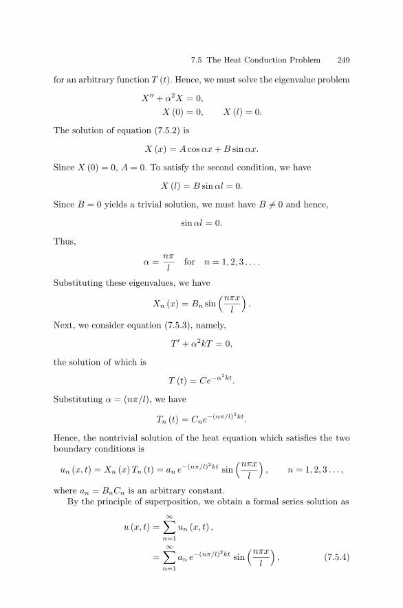
7.5 The Heat Conduction Problem 249
for an arbitrary function T (t). Hence, we must solve the eigenvalue problem
X ′′ + α2X = 0,
X (0) = 0, X (l) = 0.
The solution of equation (7.5.2) is
X (x) = A cos αx + B sin αx.
Since X (0) = 0, A = 0. To satisfy the second condition, we have
X (l) = B sin αl = 0.
Since B = 0 yields a trivial solution, we must have B = 0 and hence,
sin αl = 0.
Thus,
α =nπ
lfor n = 1, 2, 3 . . . .
Substituting these eigenvalues, we have
Xn (x) = Bn sin(nπx
l
).
Next, we consider equation (7.5.3), namely,
T ′ + α2kT = 0,
the solution of which is
T (t) = Ce−α2kt.
Substituting α = (nπ/l), we have
Tn (t) = Cne−(nπ/l)2kt.
Hence, the nontrivial solution of the heat equation which satisfies the twoboundary conditions is
un (x, t) = Xn (x) Tn (t) = an e−(nπ/l)2kt sin(nπx
l
), n = 1, 2, 3 . . . ,
where an = BnCn is an arbitrary constant.By the principle of superposition, we obtain a formal series solution as
u (x, t) =∞∑
n=1
un (x, t) ,
=∞∑
n=1
an e−(nπ/l)2kt sin(nπx
l
), (7.5.4)

250 7 Method of Separation of Variables
which satisfies the initial condition if
u (x, 0) = f (x) =∞∑
n=1
an sin(nπx
l
).
This holds true if f (x) can be represented by a Fourier sine series withFourier coefficients
an =2l
∫ l
0f (x) sin
(nπx
l
)dx. (7.5.5)
Hence,
u (x, t) =∞∑
n=1
[2l
∫ l
0f (τ) sin
(nπτ
l
)dτ
]e−(nπ/l)2kt sin
(nπx
l
)(7.5.6)
is the formal series solution of the heat conduction problem.
Example 7.5.1. (a) Suppose the initial temperature distribution is f (x) =x (l − x). Then, from equation (7.5.5), we have
an =8l2
n3π3 , n = 1, 3, 5, . . . .
Thus, the solution is
u (x, t) =(
8l2
π3
) ∞∑n=1,3,5,...
1n3 e−(nπ/l)2kt sin
(nπx
l
).
(b) Suppose the temperature at one end of the rod is held constant, thatis,
u (l, t) = u0, t ≥ 0.
The problem here is
ut = k uxx, 0 < x < l, t > 0,
u (0, t) = 0, u (l, t) = u0, (7.5.7)u (x, 0) = f (x) , 0 < x < l.
Let
u (x, t) = v (x, t) +u0x
l.
Substitution of u (x, t) in equations (7.5.7) yields
vt = k vxx, 0 < x < l, t > 0,
v (0, t) = 0, v (l, t) = 0,
v (x, 0) = f (x) − u0x
l, 0 < x < l.

7.6 Existence and Uniqueness of Solution of the Heat Conduction Problem 251
Hence, with the knowledge of solution (7.5.6), we obtain the solution
u (x, t) =∞∑
n=1
[2l
∫ l
0
(f (τ) − u0τ
l
)sin
(nπτ
l
)dτ
]e−(nπ/l)2kt sin
(nπx
l
)+
(u0x
l
). (7.5.8)
7.6 Existence and Uniqueness of Solution of the HeatConduction Problem
In the preceding section, we found that (7.5.4) is the formal solution of theheat conduction problem (7.5.1), where an is given by (7.5.5).
We shall prove the existence of this formal solution if f (x) is continuousin [0, l] and f (0) = f (l) = 0, and f ′ (x) is piecewise continuous in (0, l).Since f (x) is bounded, we have
|an| =2l
∣∣∣∣∣∫ l
0f (x) sin
(nπx
l
)dx
∣∣∣∣∣ ≤ 2l
∫ l
0|f (x)| dx ≤ C,
where C is a positive constant. Thus, for any finite t0 > 0,∣∣∣an e−(nπ/l)2kt sin(nπx
l
)∣∣∣ ≤ C e−(nπ/l)2kt0 when t ≥ t0.
According to the ratio test, the series of terms exp[− (nπ/l)2 kt0
]con-
verges. Hence, by the Weierstrass M-test, the series (7.5.4) converges uni-formly with respect to x and t whenever t ≥ t0 and 0 ≤ x ≤ l.
Differentiating equation (7.5.4) termwise with respect to t, we obtain
ut = −∞∑
n=1
an
(nπ
l
)2k e−(nπ/l)2kt sin
(nπx
l
). (7.6.1)
We note that∣∣∣∣−an
(nπ
l
)2k e−(nπ/l)2kt sin
(nπx
l
)∣∣∣∣ ≤ C(nπ
l
)2k e−(nπ/l)2kt0
when t ≥ t0, and the series of terms C (nπ/l)2 k exp[− (nπ/l)2 kt0
]con-
verges by the ratio test. Hence, equation (7.6.1) is uniformly convergent inthe region 0 ≤ x ≤ l, t ≥ t0. In a similar manner, the series (7.5.4) can bedifferentiated twice with respect to x, and as a result
uxx = −∞∑
n=1
an
(nπ
l
)2e−(nπ/l)2kt sin
(nπx
l
). (7.6.2)

252 7 Method of Separation of Variables
Evidently, from equations (7.6.1) and (7.6.2),
ut = k uxx.
Hence, equation (7.5.4) is a solution of the one-dimensional heat equationin the region 0 ≤ x ≤ l, t ≥ 0.
Next, we show that the boundary conditions are satisfied. Here, we notethat the series (7.5.4) representing the function u (x, t) converges uniformlyin the region 0 ≤ x ≤ l, t ≥ 0. Since the function represented by a uniformlyconvergent series of continuous functions is continuous, u (x, t) is continuousat x = 0 and x = l. As a consequence, when x = 0 and x = l, solution(7.5.4) satisfies
u (0, t) = 0, u (l, t) = 0,
for all t > 0.It remains to show that u (x, t) satisfies the initial condition
u (x, 0) = f (x) , 0 ≤ x ≤ l.
Under the assumptions stated earlier, the series for f (x) given by
f (x) =∞∑
n=1
an sin(nπx
l
)is uniformly and absolutely convergent. By Abel’s test of convergence theseries formed by the product of the terms of a uniformly convergent series
∞∑n=1
an sin(nπx
l
)and a uniformly bounded and monotone sequence exp
[− (nπ/l)2 kt
]con-
verges uniformly with respect to t. Hence,
u (x, t) =∞∑
n=1
an e−(nπ/l)2kt sin(nπx
l
)converges uniformly for 0 ≤ x ≤ l, t ≥ 0, and by the same reasoning asbefore, u (x, t) is continuous for 0 ≤ x ≤ l, t ≥ 0. Thus, the initial condition
u (x, 0) = f (x) , 0 ≤ x ≤ l
is satisfied. The existence of solution is therefore established.In the above discussion the condition imposed on f (x) is stronger than
necessary. The solution can be obtained with a less stringent condition onf (x) (see Weinberger (1965)).

7.6 Existence and Uniqueness of Solution of the Heat Conduction Problem 253
Theorem 7.6.1. (Uniqueness Theorem) Let u (x, t) be a continuouslydifferentiable function. If u (x, t) satisfies the differential equation
ut = k uxx, 0 < x < l, t > 0,
the initial conditions
u (x, 0) = f (x) , 0 ≤ x ≤ l,
and the boundary conditions
u (0, t) = 0, u (l, t) = 0, t ≥ 0,
then, the solution is unique.
Proof. Suppose that there are two distinct solutions u1 (x, t) and u2 (x, t).Let
v (x, t) = u1 (x, t) − u2 (x, t) .
Then,
vt = k vxx, 0 < x < l, t > 0,
v (0, t) = 0, v (l, t) = 0, t ≥ 0, (7.6.3)v (x, 0) = 0, 0 ≤ x ≤ l,
Consider the function defined by the integral
J (t) =12k
∫ l
0v2dx.
Differentiating with respect to t, we have
J ′ (t) =1k
∫ l
0vvtdx =
∫ l
0vvxxdx,
by virtue of equation (7.6.3). Integrating by parts, we have∫ l
0vvxxdx = [vvx]l0 −
∫ l
0v2
xdx.
Since v (0, t) = v (l, t) = 0,
J ′ (t) = −∫ l
0v2
x dx ≤ 0.
From the condition v (x, 0) = 0, we have J (0) = 0. This condition andJ ′ (t) ≤ 0 implies that J (t) is a nonincreasing function of t. Thus,

254 7 Method of Separation of Variables
J (t) ≤ 0.
But by definition of J (t),
J (t) ≥ 0.
Hence,
J (t) = 0, for t ≥ 0.
Since v (x, t) is continuous, J (t) = 0 implies
v (x, t) = 0
in 0 ≤ x ≤ l, t ≥ 0. Therefore, u1 = u2 and the solution is unique.
7.7 The Laplace and Beam Equations
Example 7.7.1. Consider the steady state temperature distribution in a thinrectangular slab. Two sides are insulated, one side is maintained at zerotemperature, and the temperature of the remaining side is prescribed to bef (x). Thus, we are required to solve
∇2u = 0, 0 < x < a, 0 < y < b,
u (x, 0) = f (x) , 0 ≤ x ≤ a,
u (x, b) = 0, 0 ≤ x ≤ a,
ux (0, y) = 0, ux (a, y) = 0.
Let u (x, y) = X (x) Y (y). Substitution of this into the Laplace equationyields
X ′′ − λX = 0, Y ′′ + λX = 0.
Since the boundary conditions are homogeneous on x = 0 and x = a, wehave λ = −α2 with α ≥ 0 for nontrivial solutions of the eigenvalue problem
X ′′ + α2X = 0,
X ′ (0) = X ′ (a) = 0.
The solution is
X (x) = A cos αx + B sin αx.
Application of the boundary conditions then yields B = 0 and α = (nπ/a)with n = 0, 1, 2, . . .. Hence,
Xn (x) = A cos(nπx
a
).

7.7 The Laplace and Beam Equations 255
The solution of the Y equation is clearly
Y (y) = C cosh αy + D sinhαy
which can be written in the form
Y (y) = E sinhα (y + F ) ,
where E =(D2 − C2
) 12 and F =
[tanh−1 (C/D)
]/α.
Applying the homogeneous boundary condition Y (b) = 0, we obtain
Y (b) = E sinhα (b + F ) = 0
which implies
F = −b, E = 0
for nontrivial solutions. Hence, we have
u (x, y) =(b − y)
b
a0
2+
∞∑n=1
an cos(nπx
a
)sinh
nπ
a(y − b)
.
Now we apply the remaining nonhomogeneous condition to obtain
u (x, 0) = f (x) =a0
2+
∞∑n=1
an cos(nπx
a
)sinh
(−nπb
a
).
Since this is a Fourier cosine series, the coefficients are given by
a0 =2a
∫ a
0f (x) dx,
an =−2
a sinh(
nπba
) ∫ a
0f (x) cos
(nπx
a
)dx, n = 1, 2, . . . .
Thus, the solution is
u (x, y) =(
b − y
b
)a0
2+
∞∑n=1
a∗n
sinh nπa (b − y)
sinh nπba
cos(nπx
a
),
where
a∗n =
2a
∫ a
0f (x) cos
(nπx
a
)dx.
If, for example f (x) = x in 0 < x < π, 0 < y < π, then we find (note thata = π)
a0 = π, a∗n =
2πn2 [(−1)n − 1] , n = 1, 2, . . .
and hence, the solution has the final form
u (x, y) =12
(π − y) +∞∑
n=1
2πn2 [(−1)n − 1]
sinhn (π − y)sinhnπ
cos nx.

256 7 Method of Separation of Variables
Example 7.7.2. As another example, we consider the transverse vibrationof a beam. The equation of motion is governed by
utt + a2uxxxx = 0, 0 < x < l, t > 0,
where u (x, t) is the displacement and a is the physical constant. Note thatthe equation is of the fourth order in x. Let the initial and boundary con-ditions be
u (x, 0) = f (x) , 0 ≤ x ≤ l,
ut (x, 0) = g (x) , 0 ≤ x ≤ l,
u (0, t) = u (l, t) = 0, t > 0, (7.7.1)uxx (0, t) = uxx (l, t) = 0, t > 0.
The boundary conditions represent the beam being simple supported, thatis, the displacements and the bending moments at the ends are zero.
Assume a nontrivial solution in the form
u (x, t) = X (x) T (t) ,
which transforms the equation of motion into the forms
T ′′ + a2α4T = 0, X(iv) − α4X = 0, α > 0.
The equation for X (x) has the general solution
X (x) = A cosh αx + B sinhαx + C cos αx + D sin αx.
The boundary conditions require that
X (0) = X (l) = 0, X ′′ (0) = X ′′ (l) = 0.
Differentiating X twice with respect to x, we obtain
X ′′ (x) = Aα2 cosh αx + Bα2 sinhαx − Cα2 cos αx − Dα2 sin αx.
Now applying the conditions X (0) = X ′′ (0) = 0, we obtain
A + C = 0, α2 (A − C) = 0,
and hence,
A = C = 0.
The conditions X (l) = X ′′ (l) = 0 yield
B sinhαl + D sin αl = 0,
B sinhαl − D sin αl = 0.

7.7 The Laplace and Beam Equations 257
These equations are satisfied if
B sinhαl = 0, D sin αl = 0.
Since sinhαl = 0, B must vanish. For nontrivial solutions, D = 0,
sin αl = 0,
and hence,
α =(nπ
l
), n = 1, 2, 3, . . . .
We then obtain
Xn (x) = Dn sin(nπx
l
).
The general solution for T (t) is
T (t) = E cos(aα2t
)+ F sin
(aα2t
).
Inserting the values of α2, we obtain
Tn (t) = En cos
a(nπ
l
)2t
+ Fn sin
a(nπ
l
)2t
.
Thus, the general solution for the transverse vibrations of a beam is
u (x, t) =∞∑
n=1
[an cos
a(nπ
l
)2t
+ bn sin
a(nπ
l
)2t
]sin
(nπx
l
).
(7.7.2)To satisfy the initial condition u (x, 0) = f (x), we must have
u (x, 0) = f (x) =∞∑
n=1
an sin(nπx
l
)from which we find
an =2l
∫ l
0f (x) sin
(nπx
l
)dx. (7.7.3)
Now the application of the second initial condition gives
ut (x, 0) = g (x) =∞∑
n=1
bna(nπ
l
)2sin
(nπx
l
)and hence,
bn =2al
(l
nπ
)2 ∫ l
0g (x) sin
(nπx
l
)dx. (7.7.4)
Thus, the solution of the initial boundary-value problem is given by equa-tions (7.7.2)–(7.7.4).

258 7 Method of Separation of Variables
7.8 Nonhomogeneous Problems
The partial differential equations considered so far in this chapter are homo-geneous. In practice, there is a very important class of problems involvingnonhomogeneous equations. First, we shall illustrate a problem involving atime-independent nonhomogeneous equations.
Example 7.8.1. Consider the initial boundary-value problem
utt = c2uxx + F (x) , 0 < x < l, t > 0,
u (x, 0) = f (x) , 0 ≤ x ≤ l,
ut (x, 0) = g (x) , 0 ≤ x ≤ l, (7.8.1)u (0, t) = A, u (l, t) = B, t > 0.
We assume a solution in the form
u (x, t) = v (x, t) + U (x) .
Substitution of u (x, t) in equation (7.8.1) yields
vtt = c2 (vxx + Uxx) + F (x) ,
and if U (x) satisfies the equation
c2Uxx + F (x) = 0,
then v (x, t) satisfies the wave equation
vtt = c2vxx.
In a similar manner, if u (x, t) is inserted in the initial and boundary con-ditions, we obtain
u (x, 0) = v (x, 0) + U (x) = f (x) ,
ut (x, 0) = vt (x, 0) = g (x) ,
u (0, t) = v (0, t) + U (0) = A,
u (l, t) = v (l, t) + U (l) = B .
Thus, if U (x) is the solution of the problem
c2Uxx + F = 0,
U (0) = A, U (l) = B,
then v (x, t) must satisfy
vtt = c2vxx,
v (x, 0) = f (x) − U (x) ,
vt (x, 0) = g (x) , (7.8.2)v (0, t) = 0, v (l, t) = 0.

7.8 Nonhomogeneous Problems 259
Now v (x, t) can be solved easily since U (x) is known. It can be seen that
U (x) = A + (B − A)x
l+
x
l
∫ l
0
[1c2
∫ η
0F (ξ) dξ
]dη
−∫ x
0
[1c2
∫ η
0F (ξ) dξ
]dη.
As a specific example, consider the problem
utt = c2uxx + h, h is a constantu (x, 0) = 0, ut (x, 0) = 0, (7.8.3)u (0, t) = 0, u (l, t) = 0.
Then, the solution of the system
c2Uxx + h = 0,
U (0) = 0, U (l) = 0,
is
U (x) =h
2c2
(lx − x2) .
The function v (x, t) must satisfy
vtt = c2vxx,
v (x, 0) = − h
2c2
(lx − x2) , vt (x, 0) = 0,
v (0, t) = 0, v (l, t) = 0.
The solution is given (see Section 7.3 with g (x) = 0) by
v (x, t) =∞∑
n=1
an cos(nπc
lt)
sin(nπx
l
),
and the coefficient is
an =2l
∫ l
0
[− h
2c2
(lx − x2)] sin
(nπx
l
)dx
an = − 4l2h
n3π3c2 for n odd
an = 0 for n even.
The solution of the given initial boundary-value problem is, therefore, givenby

260 7 Method of Separation of Variables
u (x, t) = v (x, t) + U (x)
=hx
2c2 (l − x) +∞∑
n=1
(− 4l2h
c2π3
)cos (2n − 1) (πct/l)
(2n − 1)3
× sin (2n − 1) (πx/l) . (7.8.4)
Let us now consider the problem of a finite string with an external forceacting on it. If the ends are fixed, we have
utt − c2uxx = h (x, t) , 0 < x < l, t > 0,
u (x, 0) = f (x) , 0 ≤ x ≤ l,
ut (x, 0) = g (x) , 0 ≤ x ≤ l, (7.8.5)u (0, t) = 0, u (l, t) = 0, t ≥ 0.
We assume a solution involving the eigenfunctions, sin (nπx/l), of the as-sociated eigenvalue problem in the form
u (x, t) =∞∑
n=1
un (t) sin(nπx
l
), (7.8.6)
where the functions un (t) are to be determined. It is evident that theboundary conditions are satisfied. Let us also assume that
h (x, t) =∞∑
n=1
hn (t) sin(nπx
l
). (7.8.7)
Thus,
hn (t) =2l
∫ l
0h (x, t) sin
(nπx
l
)dx. (7.8.8)
We assume that the series (7.8.6) is convergent. We then find utt anduxx from (7.8.6) and substitution of these values into (7.8.5) yields
∞∑n=1
[u′′
n (t) + λ2n un (t)
]sin
(nπx
l
)=
∞∑n=1
hn (t) sin(nπx
l
),
where λn = (nπc/l). Multiplying both sides of this equation by sin (mπx/l),where m = 1, 2, 3, . . ., and integrating from x = 0 to x = l, we obtain
u′′n (t) + λ2
n un (t) = hn (t)
the solution of which is given by
un (t) = an cos λnt + bn sin λnt +1λn
∫ t
0hn (τ) sin [λn (t − τ)] dτ. (7.8.9)

7.8 Nonhomogeneous Problems 261
Hence, the formal solution (7.8.6) takes the final form
u (x, t) =∞∑
n=1
an cos λnt + bn sin λnt
+1λn
∫ t
0hn (τ) sin [λn (t − τ)] dτ
· sin
(nπx
l
). (7.8.10)
Applying the initial conditions, we have
u (x, 0) = f (x) =∞∑
n=1
an sin(nπx
l
).
Thus,
an =2l
∫ l
0f (x) sin
(nπx
l
)dx. (7.8.11)
Similarly,
ut (x, 0) = g (x) =∞∑
n=1
bnλn sin(nπx
l
).
Thus,
bn =(
2lλn
)∫ l
0g (x) sin
(nπx
l
)dx. (7.8.12)
Hence, the formal solution of the initial boundary-value problem (7.8.5) isgiven by (7.8.10) with an given by (7.8.11) and bn given by (7.8.12).
Example 7.8.2. Determine the solution of the initial boundary-value prob-lem
utt − uxx = h, 0 < x < 1, t > 0, h = constant,u (x, 0) = x (1 − x) , 0 ≤ x ≤ 1,
ut (x, 0) = 0, 0 ≤ x ≤ 1, (7.8.13)u (0, t) = 0, u (1, t) = 0, t ≥ 0.
In this case, c = 1, λn = nπ, bn = 0 and an is given by
an = 2∫ 1
0x (1 − x) sinnπx dx =
4(nπ)3
[1 − (−1)n] .
We also have
hn = 2∫ 1
0h sin
(nπx
l
)dx =
2h
nπ[1 − (−1)n] .

262 7 Method of Separation of Variables
Hence, the integral term in (7.8.9) represents φn (t) given by
φn (t) =1λn
∫ t
0hn (τ) sin [λn (t − τ)] dτ =
2h
nπλ2n
[1 − (−1)n] (1 − cos λnt) .
The solution (7.8.10) is thus given by
u (x, t) =∞∑
n=1
4
n3π3 [1 − (−1)n] cos nπt
+2h
n3π3 [1 − (−1)n] (1 − cos nπt)
· sin nπx. (7.8.14)
We have treated the initial boundary-value problem with the fixed endconditions. Problems with other boundary conditions can also be solved ina similar manner.
We will now consider the initial boundary-value problem with time-dependent boundary conditions, namely,
utt − uxx = h (x, t) , 0 < x < l, t > 0,
u (x, 0) = f (x) , 0 ≤ x ≤ l,
ut (x, 0) = g (x) , 0 ≤ x ≤ l, (7.8.15)u (0, t) = p (t) , u (l, t) = q (t) , t ≥ 0.
We assume a solution in the form
u (x, t) = v (x, t) + U (x, t) . (7.8.16)
Substituting this into equation (7.8.15), we obtain
vtt − c2vxx = h − Utt + c2Uxx.
For the initial and boundary conditions, we have
v (x, 0) = f (x) − U (x, 0) ,
vt (x, 0) = g (x) − Ut (x, 0) ,
v (0, t) = p (t) − U (0, t) ,
v (l, t) = q (t) − U (l, t) .
In order to make the boundary conditions homogeneous, we set
U (0, t) = p (t) , U (l, t) = q (t) .
Thus, U (x, t) must take the form
U (x, t) = p (t) +x
l[q (t) − p (t)] . (7.8.17)

7.8 Nonhomogeneous Problems 263
The problem now is to find the function v (x, t) which satisfies
vtt − c2vxx = h − Utt = H (x, t) ,
v (x, 0) = f (x) − U (x, 0) = F (x) ,
vt (x, 0) = g (x) − Ut (x, 0) = G (x) , (7.8.18)v (0, t) = 0, v (l, t) = 0.
This is the same type of problem as the one with homogeneous boundarycondition that has previously been treated.
Example 7.8.3. Find the solution of the problem
utt − uxx = h, 0 < x < 1, t > 0, h = constant,u (x, 0) = x (1 − x) , 0 ≤ x ≤ 1,
ut (x, 0) = 0, 0 ≤ x ≤ 1, (7.8.19)u (0, t) = t, u (1, t) = sin t, t ≥ 0.
In this case, we use (7.8.16) and (7.8.17) with c = 1 and λn = nπ sothat
u (x, t) = v (x, t) + U (x, t) , U (x, t) = t + x (sin t − t) . (7.8.20)
Then, v must satisfy
vtt − vxx = h + x sin t,
v (x, 0) = x (1 − x) ,
vt (x, 0) = −1, (7.8.21)v (0, t) = 0, v (1, t) = 0.
It follows from (7.8.8) that
hn (t) = 2∫ 1
0(h + x sin t) sinnπx dx
=2h
nπ[1 − (−1)n] +
2 (−1)n+1
nπsin t = a + b sin t (say). (7.8.22)
We also find
an = 2∫ 1
0x (1 − x) sinnπx dx =
4(nπ)3
[1 − (−1)n] ,
and
bn =2
nπ
∫ 1
0sin nπx dx =
2(nπ)2
[1 − (−1)n] .

264 7 Method of Separation of Variables
Then, we determine the integral term in (7.8.9) so that
φn (t) =1
nπ
∫ t
0(a + b sin τ) sin [nπ (t − τ)] dτ
=1
nπ
a
nπ(1 − cos nπt) +
b
4[(sin 2t − 2t) cos nπt
− (cos 2t − 1) sinnπt]
. (7.8.23)
Hence, the solution of the problem (7.8.21) is
v (x, t) =∞∑
n=1
[an cos nπt + bn sin nπt + φn (t)] sinnπx. (7.8.24)
Thus, the solution of problem (7.8.19) is given by
u (x, t) = v (x, t) + U (x, t) ,
where v (x, t) is given by (7.8.24) and U (x, t) is given by (7.8.20)
Example 7.8.4. Use the method of separation of variables to derive the Her-mite equation from the Fokker–Planck equation of nonequilibrium statisticalmechanics
ut − uxx = (x u)x . (7.8.25)
We seek a nontrivial separable solution u (x, t) = X (x) T (t) so thatequation (7.8.25) reduces to a pair of ordinary differential equations
X ′′ + xX ′ + (1 + n) X = 0 and T ′ + nT = 0, (7.8.26ab)
where (−n) is a separation constant.We next use
X (x) = exp(
−12x2
)f (x) (7.8.27)
and rescale the independent variable to obtain the Hermite equation for fin the form
d2f
dξ2 − 2ξdf
dξ+ 2nf = 0.
The solution of (7.8.26b) gives
T (t) = cn exp (−nt) , (7.8.28)
where the coefficients cn are constants.

7.9 Exercises 265
Thus, the solution of the Fokker–Planck equation is given by
u (x, t) =∞∑
n=1
an exp(
−nt − 12x2
)Hn
(x√2
), (7.8.29)
where Hn is the Hermite function and an are arbitrary constants to bedetermined from the given initial condition
u (x, 0) = f (x) . (7.8.30)
We make the change of variables
ξ = x et and u = etv, (7.8.31)
in equation (7.8.25). Consequently, equation (7.8.25) becomes
∂v
∂t= e2t ∂2v
∂ξ2 . (7.8.32)
Making another change of variable t to τ (t), we transform (7.8.32) into thelinear diffusion equation
∂v
∂τ=
∂2v
∂ξ2 . (7.8.33)
Finally, we note that the asymptotic behavior of the solution u (x, t) ast → ∞ is of special interest. The reader is referred to Reif (1965) for suchbehavior.
7.9 Exercises
1. Solve the following initial boundary-value problems:
(a) utt = c2uxx, 0 < x < 1, t > 0,
u (x, 0) = x (1 − x), ut (x, 0) = 0, 0 ≤ x ≤ 1,
u (0, t) = u (1, t) = 0, t > 0.
(b) utt = c2uxx, 0 < x < π, t > 0,
u (x, 0) = 3 sinx, ut (x, 0) = 0, 0 ≤ x ≤ π,
u (0, t) = u (1, t) = 0, t > 0.

266 7 Method of Separation of Variables
2. Determine the solutions of the following initial boundary-value prob-lems:
(a) utt = c2uxx, 0 < x < π, t > 0,
u (x, 0) = 0, ut (x, 0) = 8 sin2 x, 0 ≤ x ≤ π,
u (0, t) = u (π, t) = 0, t > 0.
(b) utt = c2uxx = 0, 0 < x < 1, t > 0,
u (x, 0) = 0, ut (x, 0) = x sin πx, 0 ≤ x ≤ 1,
u (0, t) = u (1, t) = 0, t > 0.
3. Find the solution of each of the following problems:
(a) utt = c2uxx = 0, 0 < x < 1, t > 0,
u (x, 0) = x (1 − x), ut (x, 0) = x − tan πx4 , 0 ≤ x ≤ 1,
u (0, t) = u (π, t) = 0, t > 0.
(b) utt = c2uxx = 0, 0 < x < π, t > 0,
u (x, 0) = sinx, ut (x, 0) = x2 − πx, 0 ≤ x ≤ π,
u (0, t) = u (π, t) = 0, t > 0.
4. Solve the following problems:
(a) utt = c2uxx = 0, 0 < x < π, t > 0,
u (x, 0) = x + sin x, ut (x, 0) = 0, 0 ≤ x ≤ π,
u (0, t) = ux (π, t) = 0, t > 0.
(b) utt = c2uxx = 0, 0 < x < π, t > 0,
u (x, 0) = cos x, ut (x, 0) = 0, 0 ≤ x ≤ π,
ux (0, t) = 0, ux (π, t) = 0, t > 0.

7.9 Exercises 267
5. By the method of separation of variables, solve the telegraph equation:
utt + aut + bu = c2uxx, 0 < x < l, t > 0,
u (x, 0) = f (x) , ut (x, 0) = 0,
u (0, t) = u (l, t) = 0, t > 0.
6. Obtain the solution of the damped wave motion problem:
utt + aut = c2uxx, 0 < x < l, t > 0,
u (x, 0) = 0, ut (x, 0) = g (x) ,
u (0, t) = u (l, t) = 0.
7. The torsional oscillation of a shaft of circular cross section is governedby the partial differential equation
θtt = a2θxx,
where θ (x, t) is the angular displacement of the cross section and a isa physical constant. The ends of the shaft are fixed elastically, that is,
θx (0, t) − h θ (0, t) = 0, θx (l, t) + h θ (l, t) = 0.
Determine the angular displacement if the initial angular displacementis f (x).
8. Solve the initial boundary-value problem of the longitudinal vibrationof a truncated cone of length l and base of radius a. The equation ofmotion is given by(
1 − x
h
)2 ∂2u
∂t2= c2 ∂
∂x
[(1 − x
h
)2 ∂u
∂x
], 0 < x < l, t > 0,
where c2 = (E/ρ), E is the elastic modulus, ρ is the density of thematerial and h = la/ (a − l). The two ends are rigidly fixed. If theinitial displacement is f (x), that is, u (x, 0) = f (x), find u (x, t).
9. Establish the validity of the formal solution of the initial boundary-value problems:
utt = c2uxx, 0 < x < π, t > 0,
u (x, 0) = f (x) , ut (x, 0) = g (x) , 0 ≤ x ≤ π,
ux (0, t) = 0, ux (π, t) = 0, t > 0.
10. Prove the uniqueness of the solution of the initial boundary-value prob-lem:
utt = c2uxx, 0 < x < π, t > 0,
u (x, 0) = f (x) , ut (x, 0) = g (x) , 0 ≤ x ≤ π,
ux (0, t) = 0, ux (π, t) = 0, t > 0.
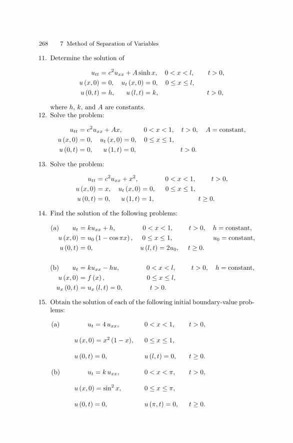
268 7 Method of Separation of Variables
11. Determine the solution of
utt = c2uxx + A sinhx, 0 < x < l, t > 0,
u (x, 0) = 0, ut (x, 0) = 0, 0 ≤ x ≤ l,
u (0, t) = h, u (l, t) = k, t > 0,
where h, k, and A are constants.12. Solve the problem:
utt = c2uxx + Ax, 0 < x < 1, t > 0, A = constant,u (x, 0) = 0, ut (x, 0) = 0, 0 ≤ x ≤ 1,
u (0, t) = 0, u (1, t) = 0, t > 0.
13. Solve the problem:
utt = c2uxx + x2, 0 < x < 1, t > 0,
u (x, 0) = x, ut (x, 0) = 0, 0 ≤ x ≤ 1,
u (0, t) = 0, u (1, t) = 1, t ≥ 0.
14. Find the solution of the following problems:
(a) ut = kuxx + h, 0 < x < 1, t > 0, h = constant,u (x, 0) = u0 (1 − cos πx) , 0 ≤ x ≤ 1, u0 = constant,u (0, t) = 0, u (l, t) = 2u0, t ≥ 0.
(b) ut = kuxx − hu, 0 < x < l, t > 0, h = constant,u (x, 0) = f (x) , 0 ≤ x ≤ l,
ux (0, t) = ux (l, t) = 0, t > 0.
15. Obtain the solution of each of the following initial boundary-value prob-lems:
(a) ut = 4uxx, 0 < x < 1, t > 0,
u (x, 0) = x2 (1 − x), 0 ≤ x ≤ 1,
u (0, t) = 0, u (l, t) = 0, t ≥ 0.
(b) ut = k uxx, 0 < x < π, t > 0,
u (x, 0) = sin2 x, 0 ≤ x ≤ π,
u (0, t) = 0, u (π, t) = 0, t ≥ 0.
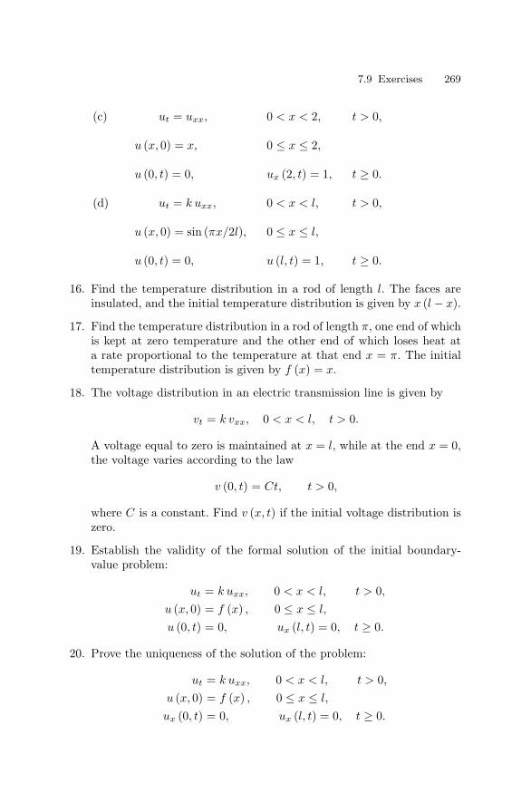
7.9 Exercises 269
(c) ut = uxx, 0 < x < 2, t > 0,
u (x, 0) = x, 0 ≤ x ≤ 2,
u (0, t) = 0, ux (2, t) = 1, t ≥ 0.
(d) ut = k uxx, 0 < x < l, t > 0,
u (x, 0) = sin (πx/2l), 0 ≤ x ≤ l,
u (0, t) = 0, u (l, t) = 1, t ≥ 0.
16. Find the temperature distribution in a rod of length l. The faces areinsulated, and the initial temperature distribution is given by x (l − x).
17. Find the temperature distribution in a rod of length π, one end of whichis kept at zero temperature and the other end of which loses heat ata rate proportional to the temperature at that end x = π. The initialtemperature distribution is given by f (x) = x.
18. The voltage distribution in an electric transmission line is given by
vt = k vxx, 0 < x < l, t > 0.
A voltage equal to zero is maintained at x = l, while at the end x = 0,the voltage varies according to the law
v (0, t) = Ct, t > 0,
where C is a constant. Find v (x, t) if the initial voltage distribution iszero.
19. Establish the validity of the formal solution of the initial boundary-value problem:
ut = k uxx, 0 < x < l, t > 0,
u (x, 0) = f (x) , 0 ≤ x ≤ l,
u (0, t) = 0, ux (l, t) = 0, t ≥ 0.
20. Prove the uniqueness of the solution of the problem:
ut = k uxx, 0 < x < l, t > 0,
u (x, 0) = f (x) , 0 ≤ x ≤ l,
ux (0, t) = 0, ux (l, t) = 0, t ≥ 0.

270 7 Method of Separation of Variables
21. Solve the radioactive decay problem:
ut − k uxx = Ae−ax, 0 < x < π, t > 0,
u (x, 0) = sinx, 0 ≤ x ≤ π,
u (0, t) = 0, u (π, t) = 0, t ≥ 0.
22. Determine the solution of the initial boundary-value problem:
ut − k uxx = h (x, t) , 0 < x < l, t > 0, k = constant,u (x, 0) = f (x) , 0 ≤ x ≤ l,
u (0, t) = p (t) , u (l, t) = q (t) , t ≥ 0.
23. Determine the solution of the initial boundary-value problem:
ut − k uxx = h (x, t) , 0 < x < l, t > 0,
u (x, 0) = f (x) , 0 ≤ x ≤ l,
u (0, t) = p (t) , ux (l, t) = q (t) , t ≥ 0.
24. Solve the problem:
ut − k uxx = 0, 0 < x < 1, t > 0,
u (x, 0) = x (1 − x) , 0 ≤ x ≤ 1,
u (0, t) = t, u (1, t) = sin t, t ≥ 0.
25. Solve the problem:
ut − 4uxx = xt, 0 < x < 1, t ≥ 0,
u (x, 0) = sinπx, 0 ≤ x ≤ 1,
u (0, t) = t, u (1, t) = t2, t ≥ 0.
26. Solve the problem:
ut − k uxx = x cos t, 0 < x < π, t > 0,
u (x, 0) = sinx, 0 ≤ x ≤ π,
u (0, t) = t2, u (π, t) = 2t, t ≥ 0.
27. Solve the problem:
ut − uxx = 2x2t, 0 < x < 1, t > 0,
u (x, 0) = cos (3πx/2) , 0 ≤ x ≤ 1,
u (0, t) = 1, ux (1, t) =3π
2, t ≥ 0.
28. Solve the problem:
ut − 2 uxx = h, 0 < x < 1, t > 0, h = constant,u (x, 0) = x, 0 ≤ x ≤ 1,
u (0, t) = sin t, ux (1, t) + u (1, t) = 2, t ≥ 0.

7.9 Exercises 271
29. Determine the solution of the initial boundary-value problem:
utt − c2uxx = h (x, t) , 0 < x < l, t > 0,
u (x, 0) = f (x) , 0 ≤ x ≤ l,
ut (x, 0) = g (x) , 0 ≤ x ≤ l,
u (0, t) = p (t) , ux (l, t) = q (t) , t ≥ 0.
30. Determine the solution of the initial boundary-value problem:
utt − c2uxx = h (x, t) , 0 < x < l, t > 0,
u (x, 0) = f (x) , 0 ≤ x ≤ l,
ut (x, 0) = g (x) , 0 ≤ x ≤ l,
ux (0, t) = p (t) , ux (l, t) = q (t) , t ≥ 0.
31. Solve the problem:
utt − uxx = 0, 0 < x < 1, t > 0,
u (x, 0) = x, ut (x, 0) = 0, 0 ≤ x ≤ 1,
u (0, t) = t2, u (1, t) = cos t, t ≥ 0.
32. Solve the problem:
utt − 4 uxx = xt, 0 < x < 1, t > 0,
u (x, 0) = x, ut (x, 0) = 0, 0 ≤ x ≤ 1,
u (0, t) = 0, ux (1, t) = 1 + t, t ≥ 0.
33. Solve the problem:
utt − 9 uxx = 0, 0 < x < 1, t > 0,
u (x, 0) = sin(πx
2
), ut (x, 0) = 1 + x, 0 ≤ x ≤ 1,
ux (0, t) = π/2, ux (1, t) = 0, t ≥ 0.
34. Find the solution of the problem:
utt + 2k ut − c2uxx = 0, 0 < x < l, t > 0,
u (x, 0) = 0, ut (x, 0) = 0, 0 ≤ x ≤ l,
ux (0, t) = 0, u (l, t) = h, t ≥ 0, h = constant.
35. Solve the problem:
ut − c2uxx + hu = hu0, −π < x < π, t > 0,
u (x, 0) = f (x) , −π ≤ x ≤ π,
u (−π, t) = u (π, t) , ux (−π, t) = ux (π, t) , t ≥ 0,
where h and u0 are constants.

272 7 Method of Separation of Variables
36. Prove the uniqueness theorem for the boundary-value problem involvingthe Laplace equation:
uxx + uyy = 0, 0 < x < a, 0 < y < b,
u (x, 0) = f (x) , u (x, b) = 0, 0 ≤ x ≤ a,
ux (0, y) = 0 = ux (a, y) , 0 ≤ y ≤ b.
37. Consider the telegraph equation problem:
utt − c2uxx + aut + bu = 0, 0 < x < l, t > 0,
u (x, 0) = f (x) , ut (x, 0) = g (x) for 0 ≤ x ≤ l,
u (0, t) = 0 = u (l, t) for t ≥ 0,
where a and b are positive constants.
(a) Show that, for any T > 0,∫ l
0
(u2
t + c2u2x + bu2)
t=Tdx ≤
∫ l
0
(u2
t + c2u2x + bu2)
t=0 dx.
(b) Use the above integral inequality from (a) to show that the initialboundary-value problem for the telegraph equation can have only onesolution.

8
Eigenvalue Problems and Special Functions
“The tool which serves as intermediary between theory and practice, be-tween thought and observation, is mathematics; it is mathematics whichbuilds the linking bridges and gives the ever more reliable forms. From thisit has come about that our entire contemporary culture, in as much as itis based on the intellectual penetration and the exploitation of nature, hasits foundations in mathematics.”
David Hilbert
“In 1836/7, he published some important joint work with his friend Sturmon what became known as Sturm–Liouville theory, which became importantin physics.”
Ioan James
8.1 Sturm–Liouville Systems
In the preceding chapter, we determined the solutions of partial differen-tial equations by the method of separation of variables. In this chapter, wegeneralize the method of separation of variables and the associated eigen-value problems. This generalization, usually known as the Sturm–Liouvilletheory, greatly extends the scope of the method of separation of variables.
Under separable conditions we transformed the second-order homoge-neous partial differential equation into two ordinary differential equations(7.2.11) and (7.2.12) which are of the form
a1 (x)d2y
dx2 + a2 (x)dy
dx+ [a3 (x) + λ] y = 0. (8.1.1)
If we introduce

274 8 Eigenvalue Problems and Special Functions
p (x) = exp[∫ x a2 (t)
a1 (t)dt
], q (x) =
a3 (x)a1 (x)
p (x) , s (x) =p (x)a1 (x)
, (8.1.2)
into equation (8.1.1), we obtain
d
dx
(p
dy
dx
)+ (q + λ s) y = 0, (8.1.3)
which is known as the Sturm–Liouville equation. In terms of the Sturm–Liouville operator
L ≡ d
dx
(p
d
dx
)+ q,
equation (8.1.3) can be written as
L [y] + λ s (x) y = 0, (8.1.4)
where λ is a parameter independent of x, and p, q, and s are real-valuedfunctions of x. To ensure the existence of solutions, we let q and s becontinuous and p be continuously differentiable in a closed finite interval[a, b].
The Sturm–Liouville equation is called regular in the interval [a, b] ifthe functions p (x) and s (x) are positive in the interval [a, b]. Thus, for agiven λ, there exist two linearly independent solutions of a regular Sturm–Liouville equation in the interval [a, b].
The Sturm–Liouville equation
L [y] + λ s (x) y = 0, a ≤ x ≤ b,
together with the separated end conditions
a1y (a) + a2y′ (a) = 0, b1y (b) + b2y
′ (b) = 0, (8.1.5)
where a1 and a2, and likewise b1 and b2, are not both zero and are givenreal numbers, is called a regular Sturm–Liouville (RSL) system.
The values of λ for which the Sturm–Liouville system has a nontrivialsolution are called the eigenvalues, and the corresponding solutions arecalled the eigenfunctions. For a regular Sturm–Liouville problem, we denotethe domain of L by D (L), that is, D (L) is the space of all complex-valuedfunctions y defined on [a, b] for which y′′ ∈ L2 ([a, b]) and which satisfyboundary conditions (8.1.5).
Example 8.1.1. Consider the regular Sturm–Liouville problem
y′′ + λy = 0, 0 ≤ x ≤ π,
y (0) = 0, y′ (π) = 0.

8.1 Sturm–Liouville Systems 275
When λ ≤ 0, it can be readily shown that λ is not an eigenvalue. How-ever, when λ > 0, the solution of the Sturm–Liouville equation is
y (x) = A cos√
λ x + B sin√
λ x.
Applying the condition y (0) = 0, we obtain A = 0. The condition y′ (π) = 0yields
B√
λ cos√
λ π = 0.
Since λ = 0 and B = 0 yields a trivial solution, we must have
cos√
λ π = 0, B = 0.
This equation is satisfied if
√λ =
2n − 12
, n = 1, 2, 3, . . . ,
and hence, the eigenvalues are λn = (2n − 1)2 /4, and the correspondingeigenfunctions are
sin(
2n − 12
)x, n = 1, 2, 3, . . . .
Example 8.1.2. Consider the Euler equation
x2y′′ + xy′ + λu = 0, 1 ≤ x ≤ e
with the end conditions
y (1) = 0, y (e) = 0.
By using the transformation (8.1.2), the Euler equation can be put intothe Sturm–Liouville form:
d
dx
(x
dy
dx
)+
1x
λ y = 0.
The solution of the Euler equation is
y (x) = c1 xi√
λ + c2 x−i√
λ.
Noting that xia = eia ln x = cos (a lnx) + i sin (a lnx), the solution y (x)becomes
y (x) = A cos(√
λ ln x)
+ B sin(√
λ ln x)
,
where A and B are constants related to c1 and c2. The end conditiony (1) = 0 gives A = 0, and the end condition y (e) = 0 gives

276 8 Eigenvalue Problems and Special Functions
sin√
λ = 0, B = 0,
which in turn yields the eigenvalues
λn = n2π2, n = 1, 2, 3, . . . ,
and the corresponding eigenfunctions
sin (nπ ln x) , n = 1, 2, 3, . . . .
Another type of problem that often occurs in practice is the periodicSturm–Liouville system.
The Sturm–Liouville equation
d
dx
(p (x)
dy
dx
)+ [q (x) + λs (x)] y = 0, a ≤ x ≤ b,
in which p (a) = p (b), together with the periodic end conditions
y (a) = y (b) , y′ (a) = y′ (b)
is called a periodic Sturm–Liouville system.
Example 8.1.3. Consider the periodic Sturm–Liouville system
y′′ + λy = 0, −π ≤ x ≤ π,
y (−π) = y (π) , y′ (−π) = y′ (π) .
Here we note that p (x) = 1, hence p (−π) = p (π). When λ > 0, we seethat the solution of the Sturm–Liouville equation is
y (x) = A cos√
λx + B sin√
λx.
Application of the periodic end conditions yields(2 sin
√λπ
)B = 0,(
2√
λ sin√
λπ)
A = 0.
Thus, to obtain a nontrivial solution, we must have
sin(√
λ)
π = 0, A = 0, B = 0.
Consequently,
λn = n2, n = 1, 2, 3, . . . .
Since sin√
λπ = 0 is satisfied for arbitrary A and B, we obtain two linearlyindependent eigenfunctions cosnx, and sinnx corresponding to the sameeigenvalue n2.
It can be readily shown that if λ < 0, the solution of the Sturm–Liouvilleequation does not satisfy the periodic end conditions. However, when λ = 0the corresponding eigenfunction is 1. Thus, the eigenvalues of the periodicSturm–Liouville system are 0,
n2
, and the corresponding eigenfunctions
are 1, cos nx, sin nx, where n is a positive integer.

8.2 Eigenvalues and Eigenfunctions 277
8.2 Eigenvalues and Eigenfunctions
In Examples 8.1.1 and 8.1.2 of the regular Sturm–Liouville systems in thepreceding section, we see that there exists only one linearly independenteigenfunction corresponding to the eigenvalue λ, which is called an eigen-value of multiplicity one (or a simple eigenvalue). An eigenvalue is said tobe of multiplicity k if there exist k linearly independent eigenfunctions cor-responding to the same eigenvalue. In Example 8.1.3 of the periodic Sturm–Liouville system, the eigenfunctions cosnx, sinnx correspond to the sameeigenvalue n2. Thus, this eigenvalue is of multiplicity two.
In the preceding examples, we see that the eigenfunctions are cos nxand sinnx for n = 1, 2, 3, . . .. It can be easily shown by using trigonometricidentities that∫ π
−π
cos mx cos nx dx = 0, m = n,∫ π
−π
cos mx sin nx dx = 0, for all integers m, n,∫ π
−π
sin mx sin nx dx = 0, m = n.
We say that these functions are orthogonal to each other in the interval[−π, π]. The orthogonality relation holds in general for the eigenfunctionsof Sturm–Liouville systems
Let φ (x) and ψ (x) be any real-valued integrable functions on an intervalI. Then φ and ψ are said to be orthogonal on I with respect to a weightfunction ρ (x) > 0, if and only if,
〈φ, ψ〉 =∫
I
φ (x) ψ (x) ρ (x) dx = 0. (8.2.1)
The interval I may be of infinite extent, or it may be either open or closedat one or both ends of the finite interval.
When φ = ψ in (8.2.1) we define the norm of φ by
‖φ‖ =[∫
I
φ2 (x) ρ (x) dx
] 12
. (8.2.2)
Theorem 8.2.1. Let the coefficients p, q, and s in the Sturm–Liouville sys-tem be continuous in [a, b]. Let the eigenfunctions φj and φk, correspondingto λj and λk, be continuously differentiable. Then φj and φk are orthogonalwith respect to the weight function s (x) in [a, b].
Proof. Since φj corresponding to λj satisfies the Sturm–Liouville equa-tion, we have
d
dx
(p φ′
j
)+ (q + λjs) φj = 0 (8.2.3)

278 8 Eigenvalue Problems and Special Functions
and for the same reason
d
dx(p φ′
k) + (q + λks) φk = 0. (8.2.4)
Multiplying equation (8.2.3) by φk and equation (8.2.4) by φj , and sub-tracting, we obtain
(λj − λk) s φjφk = φjd
dx(p φ′
k) − φkd
dx
(p φ′
j
)=
d
dx
[(p φ′
k) φj − (p φ′
j
)φk
]and integrating yields
(λj − λk)∫ b
a
s φjφkdx =[p(φjφ
′k − φ′
jφk
)]b
a
= p (b)[φj (b) φ′
k (b) − φ′j (b) φk (b)
]−p (a)
[φj (a) φ′
k (a) − φ′j (a) φk (a)
](8.2.5)
the right side of which is called the boundary term of the Sturm–Liouvillesystem. The end conditions for the eigenfunctions φj and φk are
b1φj (b) + b2φ′j (b) = 0,
b1φk (b) + b2φ′k (b) = 0.
If b2 = 0, we multiply the first condition by φk (b) and the second conditionby φj (b), and subtract to obtain[
φj (b) φ′k (b) − φ′
j (b) φk (b)]
= 0. (8.2.6)
In a similar manner, if a2 = 0, we obtain[φj (a) φ′
k (a) − φ′j (a) φk (a)
]= 0. (8.2.7)
We see by virtue of (8.2.6) and (8.2.7) that
(λj − λk)∫ b
a
s φj φk dx = 0. (8.2.8)
If λj and λk are distinct eigenvalues, then∫ b
a
s φj φk dx = 0. (8.2.9)
Theorem 8.2.2. The eigenfunctions of a periodic Sturm–Liouville systemin [a, b] are orthogonal with respect to the weight function s (x) in [a, b].
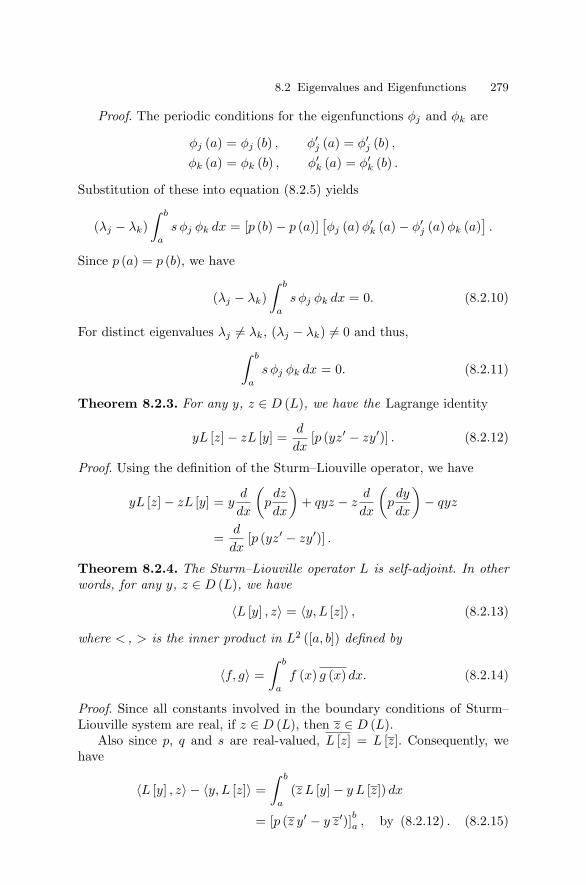
8.2 Eigenvalues and Eigenfunctions 279
Proof. The periodic conditions for the eigenfunctions φj and φk are
φj (a) = φj (b) , φ′j (a) = φ′
j (b) ,
φk (a) = φk (b) , φ′k (a) = φ′
k (b) .
Substitution of these into equation (8.2.5) yields
(λj − λk)∫ b
a
s φj φk dx = [p (b) − p (a)][φj (a) φ′
k (a) − φ′j (a) φk (a)
].
Since p (a) = p (b), we have
(λj − λk)∫ b
a
s φj φk dx = 0. (8.2.10)
For distinct eigenvalues λj = λk, (λj − λk) = 0 and thus,∫ b
a
s φj φk dx = 0. (8.2.11)
Theorem 8.2.3. For any y, z ∈ D (L), we have the Lagrange identity
yL [z] − zL [y] =d
dx[p (yz′ − zy′)] . (8.2.12)
Proof. Using the definition of the Sturm–Liouville operator, we have
yL [z] − zL [y] = yd
dx
(pdz
dx
)+ qyz − z
d
dx
(pdy
dx
)− qyz
=d
dx[p (yz′ − zy′)] .
Theorem 8.2.4. The Sturm–Liouville operator L is self-adjoint. In otherwords, for any y, z ∈ D (L), we have
〈L [y] , z〉 = 〈y, L [z]〉 , (8.2.13)
where < , > is the inner product in L2 ([a, b]) defined by
〈f, g〉 =∫ b
a
f (x) g (x) dx. (8.2.14)
Proof. Since all constants involved in the boundary conditions of Sturm–Liouville system are real, if z ∈ D (L), then z ∈ D (L).
Also since p, q and s are real-valued, L [z] = L [z]. Consequently, wehave
〈L [y] , z〉 − 〈y, L [z]〉 =∫ b
a
(z L [y] − y L [z]) dx
= [p (z y′ − y z′)]ba , by (8.2.12) . (8.2.15)

280 8 Eigenvalue Problems and Special Functions
We next show that the right hand side of this equality vanishes for aregular RSL system. If p (a) = 0, the result follows immediately. If p (a) > 0,then y and z satisfy the boundary conditions of the form (8.1.5) at x = a.That is, ⎡⎣ y (a) y′ (a)
z (a) z′ (a)
⎤⎦⎡⎣a1
a2
⎤⎦ = 0.
Since a1 and a2 are not both zero, we have
z (a) y′ (a) − y (a) z′ (a) = 0.
A similar argument can be used to the other end point x = b, so that theright-hand side of (8.2.15) vanishes. This proves the theorem.
Theorem 8.2.5. All the eigenvalues of a regular Sturm–Liouville systemwith s (x) > 0 are real.
Proof. Let λ be an eigenvalue of a RSL system and let y (x) be thecorresponding eigenfunction. This means that y = 0 and L [y] = −λsy.Then
0 = 〈L [y] , y〉 − 〈y, L [y]〉 =(λ − λ
) ∫ b
a
s (x) |y (x)|2 dx.
Since s (x) > 0 in [a, b] and y = 0, the integrand is a positive number. Thus,λ = λ, and hence, the eigenvalues are real. This completes the proof.
Theorem 8.2.6. If φ1 (x) and φ2 (x) are any two solutions of the equationL [y] + λsy = 0 on [a, b], then p (x) W (x; φ1, φ2) = constant, where W isthe Wronskian.
Proof. Since φ1 and φ2 are solutions of L [y] + λsy = 0, we have
d
dx
(p
dφ1
dx
)+ (q + λs) φ1 = 0,
d
dx
(p
dφ2
dx
)+ (q + λs) φ2 = 0.
Multiplying the first equation by φ2 and the second equation by φ1, andsubtracting, we obtain
φ1d
dx
(p
dφ2
dx
)− φ2
d
dx
(p
dφ1
dx
)= 0.
Integrating this equation from a to x, we obtain
p (x) [φ1 (x) φ′2 (x) − φ′
1 (x) φ2 (x)] = p (a) [φ1 (a) φ′2 (a) − φ′
1 (a) φ2 (a)]p (x) W (x; φ, φ2) = constant. (8.2.16)
This is called Abel’s formula where W is the Wronskian.

8.2 Eigenvalues and Eigenfunctions 281
Theorem 8.2.7. An eigenfunction of a regular Sturm–Liouville system isunique except for a constant factor.
Proof. Let φ1 (x) and φ2 (x) be eigenfunctions corresponding to an eigen-value λ. Then, according to Abel’s formula (8.2.16), we have
p (x) W (x; φ1, φ2) = constant, p (x) > 0,
where W is the Wronskian. Thus, if W vanishes at a point in [a, b], it mustvanish for all x ∈ [a, b].
Since φ1 and φ2 satisfy the end condition at x = a, we have
a1φ1 (a) + a2φ′1 (a) = 0,
a1φ2 (a) + a2φ′2 (a) = 0.
Since a1 and a2 are not both zero, we have∣∣∣∣∣∣φ1 (a) φ′
1 (a)
φ1 (a) φ′2 (a)
∣∣∣∣∣∣ = W (a; φ1, φ2) = 0.
Therefore, W (x; φ1φ2) = 0 for all x ∈ [a, b], which is a sufficient conditionfor the linear dependence of two functions φ1 and φ2. Hence, φ1 (x) differsfrom φ2 (x) only by a constant factor.
Theorem 8.2.5 states that all eigenvalues of a regular Sturm–Liouvillesystem are real, but it does not guarantee that any eigenvalue exists. How-ever, it can be proved that a self-adjoint regular Sturm–Liouville systemhas a denumerably infinite number of eigenvalues. To illustrate this, weconsider the following example.
Example 8.2.1. Consider the Sturm–Liouville system
y′′ + λy = 0, 0 ≤ x ≤ 1,
y (0) = 0, y (1) + hy′ (1) = 0, h > 0 a constant.
Here p = 1, q = 0, s = 1. The solution of the Sturm–Liouville equationis
y (x) = A cos√
λx + B sin√
λx.
Since y (0) = 0, gives A = 0, we have
y (x) = B sin√
λx.
Applying the second end condition, we have
sin√
λ + h√
λ cos√
λ = 0, B = 0

282 8 Eigenvalue Problems and Special Functions
which can be rewritten as
tan√
λ = −h√
λ.
If α =√
λ is introduced in this equation, we have
tanα = −hα.
This equation does not possess an explicit solution. Thus, we determinethe solution graphically by plotting the functions ξ = tanα and ξ = −hαagainst α, as shown in Figure 8.2.1. The roots are given by the intersectionof two curves, and as is evident from the graph, there are infinitely manyroots αn for n = 1, 2, 3, . . .. To each root αn, there corresponds an eigenvalue
λn = α2n, n = 1, 2, 3, . . . .
Thus, there exists an ordered sequence of eigenvalues
λ0 < λ1 < λ2 < λ3 < . . .
with
limn→∞ λn = ∞.
The corresponding eigenfunctions are sin(√
λn x).
Figure 8.2.1 Intersection of ξ = tan α and ξ = −h α.

8.3 Eigenfunction Expansions 283
Theorem 8.2.8. A self-adjoint regular Sturm–Liouville system has an in-finite sequence of real eigenvalues
λ1 < λ2 < λ3 < . . .
with
limn→∞ λn = ∞.
For each n the corresponding eigenfunction φn (x), uniquely determined upto a constant factor, has exactly n zeros in the interval (a, b).
Proof of this theorem can be found in the book by Myint-U (1978).
8.3 Eigenfunction Expansions
A real-valued function φ (x) is said to be square-integrable with respect toa weight function ρ (x) > 0, if, on an interval I,∫
I
φ2 (x) ρ (x) dx < +∞. (8.3.1)
An immediate consequence of this definition is the Schwarz inequality∣∣∣∣∫I
φ (x) ψ (x) ρ (x) dx
∣∣∣∣2 ≤∫
I
φ2 (x) ρ (x) dx
∫I
ψ2 (x) ρ (x) dx (8.3.2)
for square-integrable functions φ (x) and ψ (x).Let φn (x), for positive integers n, be an orthogonal set of square-
integrable functions with a positive weight function ρ (x) on an intervalI. Let f (x) be a given function that can be represented by a uniformlyconvergent series of the form
f (x) =∞∑
n=1
cn φn (x) , (8.3.3)
where the coefficients cn are constants. Now multiplying both sides of (8.3.3)by φm (x) ρ (x) and integrating term by term over the interval I (uniformconvergence of the series is a sufficient condition for this), we obtain∫
I
f (x) φm (x) ρ (x) dx =∞∑
n=1
∫I
cnφn (x) φm (x) ρ (x) dx,
and hence, for n = m,∫I
f (x) φn (x) ρ (x) dx = cn
∫I
φ2n (x) ρ (x) dx.

284 8 Eigenvalue Problems and Special Functions
Thus,
cn =
∫If φn ρ dx∫
Iφ2
n ρ dx. (8.3.4)
Hence, we have the following theorem:
Theorem 8.3.1. If f is represented by a uniformly convergent series
f (x) =∞∑
n=1
cnφn (x)
on an interval I, where φn are square-integrable functions orthogonal withrespect to a positive weight function ρ (x), then cn are determined by
cn =
∫If φn ρ dx∫
Iφ2
n ρ dx.
Example 8.3.1. The Legendre polynomials Pn (x) are orthogonal with re-spect to the weight function ρ (x) = 1 on (−1, 1). If we assume that f (x)can be represented by the Fourier–Legendre series
f (x) =∞∑
n=1
cnPn (x)
then, cn are given by
cn =
∫ 1−1 f (x) Pn (x) dx∫ 1
−1 P 2n (x) dx
=(
2n + 12
)∫ 1
−1f (x) Pn (x) dx.
In the above discussion, we assumed that the given function f (x) isrepresented by a uniformly convergent series. This is rather restrictive, andwe will show in the following section that f (x) can be represented by amean-square convergent series.
8.4 Convergence in the Mean
Let φn be the set of square-integrable functions orthogonal with respectto a weight function ρ (x) on [a, b]. Let
sn (x) =n∑
k=1
ckφk (x)

8.4 Convergence in the Mean 285
be the nth partial sum of the series∞∑
k=1
ckφk (x).
Let f be a square-integrable function. The sequence sn is said toconverge in the mean to f (x) on the interval I with respect to the weightfunction ρ (x) if
limn→+∞
∫I
[f (x) − sn (x)]2 ρ (x) dx = 0. (8.4.1)
We shall now seek the coefficients ck such that sn (x) represents thebest approximation to f (x) in the sense of least squares, that is, we seekto minimize the integral
E (ck) =∫
I
[f (x) − sn (x)]2 ρ (x) dx
=∫
I
f2ρ dx − 2n∑
k=1
ck
∫I
f φk ρ dx +n∑
k=1
c2k
∫I
φ2k ρ dx. (8.4.2)
This is an extremal problem. A necessary condition on the ck for E tobe minimum is that the first partial derivatives of E with respect to thesecoefficients vanish. Thus, differentiating (8.4.2) with respect to ck, we obtain
∂E
∂ck= −2
∫I
f φk ρ dx + 2ck
∫I
φ2k ρ dx = 0 (8.4.3)
and hence,
ck =
∫If φk ρ dx∫
Iφ2
k ρ dx. (8.4.4)
Now if we complete the square, the right side of (8.4.2) becomes
E =∫
I
f2ρ dx +n∑
k=1
∫I
φ2k ρ dx
[ck −
∫If φk ρ dx∫
Iφ2
k ρ dx
]2
−n∑
k=1
(∫If φk ρ dx
)2∫Iφ2
k ρ dx.
The right side shows that E is a minimum if and only if ck is given by(8.4.4). Therefore, this choice of ck yields the best approximation to f (x)in the sense of least squares.
For series convergent in the mean to f (x), we conventionally write
f (x) ∼∞∑
k=1
ckφk (x) ,
where the coefficients ck are the generalized Fourier coefficients and theseries is the generalized Fourier series. This series may or may not be point-wise or uniformly convergent.

286 8 Eigenvalue Problems and Special Functions
8.5 Completeness and Parseval’s Equality
Substituting the Fourier coefficients (8.4.4) into (8.4.2), we obtain
∫I
(f (x) −
n∑k=1
ckφk (x)
)2
ρ (x) dx =∫
I
f2ρ dx −n∑
k=1
c2k
∫I
φ2k ρ dx.
Since the left side is nonnegative, we have
n∑k=1
c2k
∫I
φ2k ρ dx ≤
∫I
f2ρ dx. (8.5.1)
The integral on the right side is finite, and hence, the series on the left sideis bounded above for any n. Thus, as n → ∞, the inequality (8.5.1) maybe written as
∞∑k=1
c2k
∫I
φ2k ρ dx ≤
∫I
f2ρ dx. (8.5.2)
This is called Bessel’s inequality.If the series converges in the mean to f (x), that is,
limn→∞
∫I
(f (x) −
n∑k=1
ckφk (x)
)2
ρ (x) dx = 0,
then, it follows from the above derivation that
∞∑k=1
c2k
∫I
φ2kρ dx =
∫I
f2ρ dx
which is called Parseval’s equality. Sometimes it is known as the complete-ness relation. Thus, when every continuous square-integrable function f (x)can be expanded into an infinite series
f (x) =∞∑
k=1
ckφk (x) ,
the sequence of continuous square-integrable functions φk orthogonalwith respect to the weight function ρ is said to be complete.
Next we state the following theorem:
Theorem 8.5.1. The eigenfunctions of any regular Sturm–Liouville sys-tem are complete in the space of functions that are piecewise continuouson the interval [a, b] with respect to the weight function s (x). Moreover,any piecewise smooth function on [a, b] that satisfies the end conditions of

8.5 Completeness and Parseval’s Equality 287
the regular Sturm–Liouville system can be expanded in an absolutely anduniformly convergent series
f (x) =∞∑
k=1
ckφk (x) ,
where ck are given by
ck =∫ b
a
f φk s (x) dx
/∫ b
a
φ2k s (x) dx.
Proof of a more general theorem can be found in Coddington and Levinson(1955).
Example 8.5.1. Consider a cylindrical wire of length l whose surface is per-fectly insulated against the flow of heat. The end l = 0 is maintained at thezero degree temperature, while the other end radiates freely into the sur-rounding medium of zero degree temperature. Let the initial temperaturedistribution in the wire be f (x). Find the temperature distribution u (x, t).
The initial boundary-value problem is
ut = k uxx, 0 < x < l, t > 0, (8.5.3)u (x, 0) = f (x) , 0 < x ≤ l, (8.5.4)u (0, t) = 0, t > 0, (8.5.5)
hu (l, t) + u′ (l, t) = 0, t > 0, h > 0. (8.5.6)
By the method of separation of variables, we assume a nontrivial solu-tion in the form
u (x, t) = X (x) T (t)
and substituting it in the heat equation, we obtain
X ′′ + λX = 0, T ′ + kλT = 0,
where λ > 0 is a separation constant. The solution of the latter equation is
T (t) = Ce−kλt (8.5.7)
where C is an arbitrary constant. The former equation has to be solvedsubject to the boundary conditions
X (0) = 0, hX (l) + X ′ (l) = 0.
This is a Sturm–Liouville system which gives the solution with X (0) = 0
X (x) = B sin√
λx, (8.5.8)

288 8 Eigenvalue Problems and Special Functions
where B is a constant to be determined.Application of the second end condition (8.5.6) yields
h sin√
λ l +√
λ cos√
λ l = 0 for B = 0
which can be rewritten as
tan√
λ l = −√
λ/h.
If α =√
λ l is introduced in the preceding equation, we have
tanα = −a α,
where a = (1/hl). As in Example 8.2.1, there exists a sequence of eigenval-ues
λ1 < λ2 < λ3 < . . .
with limn→∞ λn = ∞. The corresponding eigenfunctions are sin√
λn x, andhence,
Xn (x) = Bn sin√
λn x. (8.5.9)
Therefore, combining (8.5.7) with C = Cn and (8.5.9), the solution takesthe form
un (x, t) = an e−kλnt sin√
λn x, an = BnCn
which satisfies the heat equation and the boundary conditions. Since theheat equation is linear and homogeneous, we form the series solution
u (x, t) =∞∑
n=1
an e−kλnt sin√
λn x, (8.5.10)
which is also a solution, provided it converges and is twice differentiablewith respect to x and once differentiable with respect to t. According toTheorem 8.2.1, the eigenfunctions sin
√λn x form an orthogonal system
over the interval (0, l). Application of the initial condition yields
u (x, 0) = f (x) ∼∞∑
n=1
an sin√
λn x.
If we assume that f is a piecewise smooth function on [a, b], then, by Theo-rem 8.5.1, we can expand f (x) in terms of the eigenfunctions, and formallywrite
f (x) =∞∑
n=1
an sin√
λn x,
where the coefficient an is given by
an =∫ l
0f (x) sin
√λn x dx
/∫ l
0sin2
√λn x dx.
With this value of an, the temperature distribution is given by (8.5.10).

8.6 Bessel’s Equation and Bessel’s Function 289
8.6 Bessel’s Equation and Bessel’s Function
Bessel’s equation frequently occurs in problems of applied mathematics andmathematical physics involving cylindrical symmetry.
The standard form of Bessel’s equation is given by
x2y′′ + xy′ +(x2 − ν2) y = 0, (8.6.1)
where ν is a nonnegative real number. We shall first restrict our attentionto x > 0. Since x = 0 is the regular singular point, a solution is taken inaccordance with the Frobenius method to be
y (x) =∞∑
n=0
an xs+n, (8.6.2)
where the index s is to be determined. Substitution of this series into equa-tion (8.6.1) then yields(
s2 − ν2) a0 xs +[(s + 1)2 − ν2
]a1x
s+1
+∞∑
n=2
[(s + n)2 − ν2
]an + an−2
xs+n = 0. (8.6.3)
The requirement that the coefficient of xs vanish leads to the initial equation(s2 − ν2) a0 = 0, (8.6.4)
from which it follows that s = + ν for arbitrary a0 = 0. Since the leadingterm in the series (8.6.2) is a0 xs, it is clear that for ν > 0 the solution ofBessel’s equation corresponding to the choice s = ν vanishes at the origin,whereas the solution corresponding to s = −ν is infinite at that point.
We consider first the regular solution of Bessel’s equation, that is, thesolution corresponding to the choice s = ν. The vanishing of the coefficientof xs+1 in equation (8.6.3) requires that
(2ν + 1) a1 = 0, (8.6.5)
which in turn implies that a1 = 0 (since ν ≥ 0). From the requirement thatthe coefficient of xs+n in equation (8.6.3) be zero, we obtain the two-termrecurrence relation
an = − an−2
n (2ν + n). (8.6.6)
Since a1 = 0, it is obvious that an = 0 for n = 3, 5, 7, . . .. The remainingcoefficients are given by
a2k =(−1)k
a0
22kk! (ν + k) (ν + k − 1) . . . (ν + 1)(8.6.7)

290 8 Eigenvalue Problems and Special Functions
for k = 1, 2, 3, . . .. This relation may also be written as
a2k =(−1)k 2νΓ (ν + 1) a0
22k+νk!Γ (ν + k + 1), k = 1, 2, . . . , (8.6.8)
where Γ (α) is the gamma function, whose properties are described in theAppendix.
Hence, the regular solution of Bessel’s equation takes the form
y (x) = a0
∞∑k=0
(−1)k 2νΓ (ν + 1)22k+νk!Γ (ν + k + 1)
x2k+ν . (8.6.9)
It is customary to choose
a0 =1
2νΓ (ν + 1)(8.6.10)
and to denote the corresponding solution by Jν (x). This solution, calledthe Bessel function of the first kind of order ν, is therefore given by
Jν (x) =∞∑
k=0
(−1)kx2k+ν
22k+νk! Γ (ν + k + 1). (8.6.11)
To determine the irregular solution of the Bessel equation for s = −ν,we proceed as above. In this way, we obtain as the analogue of equation(8.6.5) the relation
(−2ν + 1) a1 = 0
from which it follows, without loss of generality, that a1 = 0. Using therecurrence relation
an = − an−2
n (n − 2ν), n ≥ 2 (8.6.12)
we obtain the irregular solution of the Bessel function of the first kind oforder −ν as
J−ν (x) =∞∑
k=0
(−1)kx2k−ν
22k−νk! Γ (−ν + k + 1). (8.6.13)
It can be easily proved that, if ν is not an integer, Jν and J−ν convergefor all values of x, and are linearly independent. Thus, the general solutionof the Bessel equation for nonintegral ν is
y (x) = c1Jν (x) + c2J−ν (x) . (8.6.14)
If ν is an integer, say ν = n, then from equation (8.6.13), noting that,when gamma functions in the coefficients of the first n terms become infi-nite, the coefficients become zero, hence we have

8.6 Bessel’s Equation and Bessel’s Function 291
J−n (x) =∞∑
k=n
(−1)kx2k−n
22k−nk! Γ (−n + k + 1).
= (−1)n∞∑
k=0
(−1)kx2k+n
22k+nk! Γ (n + k + 1).
= (−1)nJn (x) . (8.6.15)
This shows that J−n is not independent of Jn, and therefore, a secondlinearly independent solution is required.
A number of distinct irregular solutions are discussed in the literature,but the one most commonly used, as defined by Watson (1966), is
Yν (x) =(cos νπ) Jν (x) − J−ν (x)
sin νπ. (8.6.16)
For nonintegral ν, it is obvious that Yν (x), being a linear combination ofJν (x) and J−ν (x), is linearly independent of Jν (x). When ν is a nonneg-ative integer n, Yν (x) is indeterminate. But
Yn (x) = limν→n
Yν (x)
exists and is a solution of the Bessel equation. Moreover, it is linearly in-dependent of Jn (x). (For an extended treatment, see Watson (1966)). Thefunction Yν (x) is called the Bessel function of the second kind of order ν.Thus, the general solution of the Bessel equation is
y (x) = c1Jν (x) + c2Yν (x) , for ν ≥ 0. (8.6.17)
Like elementary functions, the Bessel functions are tabulated (see Jahnkeet al. (1960)). For illustration, the functions J0, J1, Y0 and Y1 are plottedfor small values of x in Figure 8.6.1.
It should be noted that Jν (x) for ν ≥ 0 and J−ν (x) for a positiveinteger ν are finite at the origin, but J−ν (x) for nonintegral ν and Yν (x)for ν ≥ 0 approach infinity as x tends to zero.
Some of the useful recurrence relations are
Jν−1 (x) + Jν+1 (x) =2ν
xJν (x) , (8.6.18)
νJν (x) + xJ ′ν (x) = xJν−1 (x) , (8.6.19)
Jν−1 (x) − Jν+1 (x) = 2J ′ν (x) , (8.6.20)
νJν (x) − xJ ′ν (x) = xJν+1 (x) , (8.6.21)
d
dx[xνJν (x)] = xνJν−1 (x) , (8.6.22)
d
dx
[x−νJν (x)
]= −x−νJν+1 (x) . (8.6.23)
All of these relations also hold true for Yν (x).

292 8 Eigenvalue Problems and Special Functions
Figure 8.6.1 Graphs of Jν (x) and Yν (x).
For |x| 1 and |x| ν, the asymptotic expansion of Jν (x) is
Jν−1 (x) ∼√
2πx
[1 −
(4ν2 − 12
) (4ν2 − 32
)2! (8x)2
+
(4ν2 − 12
) (4ν2 − 32
) (4ν2 − 52
) (4ν2 − 72
)4! (8x)4
− . . .
cos φ
−(
4ν2 − 12)
8x−
(4ν2 − 12
) (4ν2 − 32
) (4ν2 − 52
)3! (8x)3
+ . . .
sin φ
](8.6.24)
where
φ = x −(
ν +12
)π
2.
For |x| 1 and |x| ν, the asymptotic expansion of Yν (x) is

8.6 Bessel’s Equation and Bessel’s Function 293
Yν (x) ∼√
2πx
[1 −
(4ν2 − 12
) (4ν2 − 32
)2! (8x)2
+
(4ν2 − 12
) (4ν2 − 32
) (4ν2 − 52
) (4ν2 − 72
)4! (8x)4
− . . .
sin φ
+
(4ν2 − 12
)8x
−(4ν2 − 12
) (4ν2 − 32
) (4ν2 − 52
)3! (8x)3
+ . . .
cos φ
].
(8.6.25)
When ν = +(1/2), Bessel’s function may be expressed in the form
J 12
(x) =
√2
πxsin x, (8.6.26)
J− 12
(x) =
√2
πxcos x. (8.6.27)
The Bessel functions which satisfy the condition
Jν (akm) + hJ ′ν (akm) = 0, h, a = constant, (8.6.28)
are orthogonal to each other with respect to the weight function x, that is,for the nonnegative integer ν, the orthogonal relation is∫ a
0xJν (xkn) Jν (xkm) dx = 0, n = m. (8.6.29)
When n = m, we have the norm
‖Jν (xkm)‖2 =∫ a
0x [Jν (xkm)]2 dx
=1
2k2m
a2k2
m [J ′ν (akm)]2 +
(a2k2
m − ν2) [Jν (akm)]2
,
(8.6.30)
where km are the roots of (8.6.28).We now give a particular example of the eigenfunction expansion the-
orem discussed in Sections 8.4 and 8.5. Assume a formal expansion of thefunction f (x) defined in 0 ≤ x ≤ a in the form
f (x) =∞∑
m=1
amJν (xkm) , (8.6.31)
where the summation is taken over all the positive roots k1, k2, k3, . . .,of equation (8.6.28). Multiplying (8.6.31) by xJν (xkn), integrating, andutilizing (8.6.30), we obtain
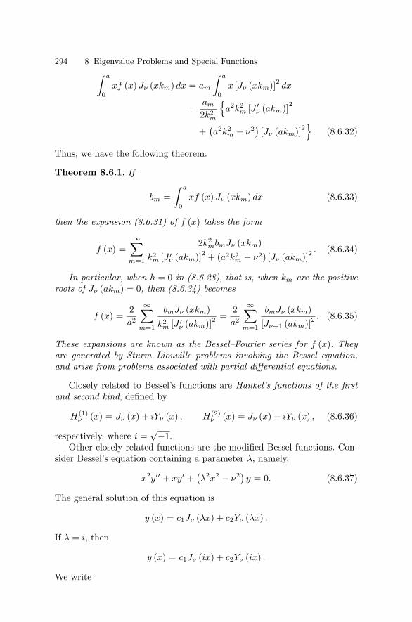
294 8 Eigenvalue Problems and Special Functions∫ a
0xf (x) Jν (xkm) dx = am
∫ a
0x [Jν (xkm)]2 dx
=am
2k2m
a2k2
m [J ′ν (akm)]2
+(a2k2
m − ν2) [Jν (akm)]2
. (8.6.32)
Thus, we have the following theorem:
Theorem 8.6.1. If
bm =∫ a
0xf (x) Jν (xkm) dx (8.6.33)
then the expansion (8.6.31) of f (x) takes the form
f (x) =∞∑
m=1
2k2mbmJν (xkm)
k2m [J ′
ν (akm)]2 + (a2k2m − ν2) [Jν (akm)]2
. (8.6.34)
In particular, when h = 0 in (8.6.28), that is, when km are the positiveroots of Jν (akm) = 0, then (8.6.34) becomes
f (x) =2a2
∞∑m=1
bmJν (xkm)k2
m [J ′ν (akm)]2
=2a2
∞∑m=1
bmJν (xkm)[Jν+1 (akm)]2
. (8.6.35)
These expansions are known as the Bessel–Fourier series for f (x). Theyare generated by Sturm–Liouville problems involving the Bessel equation,and arise from problems associated with partial differential equations.
Closely related to Bessel’s functions are Hankel’s functions of the firstand second kind, defined by
H(1)ν (x) = Jν (x) + iYν (x) , H(2)
ν (x) = Jν (x) − iYν (x) , (8.6.36)
respectively, where i =√−1.
Other closely related functions are the modified Bessel functions. Con-sider Bessel’s equation containing a parameter λ, namely,
x2y′′ + xy′ +(λ2x2 − ν2) y = 0. (8.6.37)
The general solution of this equation is
y (x) = c1Jν (λx) + c2Yν (λx) .
If λ = i, then
y (x) = c1Jν (ix) + c2Yν (ix) .
We write

8.7 Adjoint Forms and Lagrange Identity 295
Jν (ix) =∞∑
k=0
(−1)k (ix)2k+ν
22k+νk! Γ (ν + k + 1)
= iνIν (x) ,
where
Iν (x) =∞∑
k=0
x2k+ν
22k+νk! Γ (ν + k + 1), (8.6.38)
Iν (x) is called the modified Bessel function of the first kind of order ν.As in the case of Jν and J−ν , Iν and I−ν (which is defined in a similarmanner) are linearly independent solutions except when ν is an integer.Consequently, we define the modified Bessel function of the second kind oforder ν by
Kν (x) =π
2
(I−ν (x) − Iν (x)
sin νπ
). (8.6.39)
Thus, we obtain the general solution of the modified Bessel equation
x2y′′ + xy′ − (x2 + ν2) y = 0 (8.6.40)
in the form
y (x) = c1Iν (x) + c2Kν (x) . (8.6.41)
We should note that
Iν (0) =
⎧⎨⎩1, ν = 0
0, ν > 0(8.6.42)
and that Kν approaches infinity as x → 0.For a detailed treatment of Bessel and related functions, refer to Wat-
son’s (1966) Theory of Bessel Functions.The eigenvalue problems which involve Bessel’s functions will be de-
scribed in Section 8.8 on singular Sturm–Liouville systems.
8.7 Adjoint Forms and Lagrange Identity
Self-adjoint equations play a very important role in many areas of appliedmathematics and mathematical physics. Here we will give a brief accountof self-adjoint operators and the Lagrange identity.
We consider the equation
L [y] = a0 (x) y′′ + a1 (x) y′ + a2 (x) y = 0

296 8 Eigenvalue Problems and Special Functions
defined on an interval I. Integrating z (x) L [y] by parts from a to x, wehave ∫ x
a
zL [y] dx =[(za0) y′ − (za0)
′y + (za1) y
]x
a
+∫ x
a
[(za0)
′′ − (za1)′ + (za2)
]y dx. (8.7.1)
Now, if we define the second-order operator L∗ by
L∗ [z] = (za0)′′ − (za1)
′ + (za2) = a0 z′′ (2a′0 − a1) z′ + (a′′
0 − a′1 + a2) z
the relation (8.7.1) takes the form∫ x
a
(zL [y] − yL∗ [z]) dx = [a0 (y′z − yz′) + (a1 − a′0) yz]xa . (8.7.2)
The operator L∗ is called the adjoint operator corresponding to the operatorL. It can be readily verified that the adjoint of L∗ is L itself. If L and L∗ arethe same, L is said to be self-adjoint. The necessary and sufficient conditionfor this is that
a1 = 2a′0 − a1, a2 = a′′
0 − a′1 + a2,
which is satisfied if
a1 = a′0.
Thus, if L is self-adjoint, we have
L (y) = a0y′′ + a′
0y′ + a2y
= (a0y′)′ + a2 (x) y. (8.7.3)
In general, L [y] is not self-adjoint. But if we let
h (x) =1a0
exp∫ x a1 (t)
a0 (t)dt
(8.7.4)
then h (x) L [y] is self-adjoint. Thus, any second-order linear differentialequation
a0 (x) y′′ + a1 (x) y′ + a2 (x) y = 0 (8.7.5)
can be made self-adjoint. Multiplying by h (x) given by equation (8.7.4),equation (8.7.5) is transformed into the self-adjoint form
d
dx
[p (x)
dy
dx
]+ q (x) y = 0, (8.7.6)

8.8 Singular Sturm–Liouville Systems 297
where
p (x) = exp∫ x a1 (t)
a0 (t)dt
, q (x) =
(a2
a0
)exp
∫ x a1 (t)a0 (t)
dt
. (8.7.7)
For example, the self-adjoint form of the Legendre equation(1 − x2) y′′ − 2xy′ + n (n + 1) y = 0
is
d
dx
[(1 − x2) dy
dx
]+ n (n + 1) y = 0, (8.7.8)
and the self-adjoint form of the Bessel equation
x2y′′ + xy′ +(x2 − ν2) y = 0
is
d
dx
(x
dy
dx
)+
(x − ν2
x
)y = 0. (8.7.9)
Now, if we differentiate both sides of equation (8.7.2), we obtain
zL [y] − yL∗ [z] =d
dx[a0 (y′z − yz′) + (a1 − a′
0) yz] (8.7.10)
which is known as the Lagrange identity for the operator L.If we consider the integral from a to b of equation (8.7.2), we obtain
Green’s identity∫ b
a
(zL [y] − yL∗ [z]) dx = [a0 (y′z − yz′) + (a1 − a′0) yz]ba. (8.7.11)
When L is self-adjoint, this relation becomes∫ b
a
(zL [y] − yL [z]) dx = [a0 (y′z − yz′)]ba . (8.7.12)
8.8 Singular Sturm–Liouville Systems
A Sturm–Liouville equation is called singular when it is given on a semi-infinite or infinite interval, or when the coefficient p (x) or s (x) vanishes, orwhen one of the coefficients becomes infinite at one end or both ends of afinite interval. A singular Sturm–Liouville equation together with appropri-ate linear homogeneous end conditions is called a singular Sturm–Liouville(SSL) system. The conditions imposed in this case are not like the sepa-rated boundary end conditions in the regular Sturm–Liouville system. The

298 8 Eigenvalue Problems and Special Functions
condition that is often necessary to prescribe is the boundedness of thefunction y (x) at the singular end point. To exhibit this, let us consider aproblem with a singularity at the end point x = a. By the relation (8.7.12),for any twice continuously differentiable functions y (x) and z (x), we haveon (a, b)∫ b
a+ε
zL [y] − yL [z] dx = p (b) [y′ (b) z (b) − y (b) z′ (b)]
−p (a + ε) [y′ (a + ε) z (a + ε) − y (a + ε) z′ (a + ε)] ,
where ε is a small positive number. If the conditions
limx→a+
p (x) [y′ (x) z (x) − y (x) z′ (x)] = 0, (8.8.1)
p (b) [y′ (b) z (b) − y (b) z′ (b)] = 0, (8.8.2)
are imposed on y and z, it follows that∫ b
a
zL [y] − yL [z] dx = 0. (8.8.3)
For example, when p (a) = 0, the relations (8.8.1) and (8.8.2) are replacedby the conditions1. y (x) and y′ (x) are finite as x → a2. b1y (b) + b2y
′ (b) = 0.Thus, we say that the singular Sturm–Liouville system is self-adjoint, if
any functions y (x) and z (x) that satisfy the end conditions satisfy∫ b
a
zL [y] − yL [z] dx = 0.
Example 8.8.1. Consider the singular Sturm–Liouville system involving Leg-endre’s equation
d
dx
[(1 − x2) dy
dx
]+ λy = 0, −1 < x < 1,
with the conditions that y and y′ are finite as x → + 1.In this case, p (x) = 1−x2 and s (x) = 1, and p (x) vanishes at x = + 1.
The Legendre functions of the first kind, Pn (x), n = 0, 1, 2, . . ., are theeigenfunctions which are finite as x → + 1. The corresponding eigenvaluesare λn = n (n + 1) for n = 0, 1, 2, . . .. We observe here that the singu-lar Sturm–Liouville system has infinitely many real eigenvalues, and theeigenfunctions Pn (x) are orthogonal to each other.
Example 8.8.2. Another example of a singular Sturm–Liouville system isthe Bessel equation for fixed ν

8.8 Singular Sturm–Liouville Systems 299
d
dx
(x
dy
dx
)+
(λx − ν2
x
)y = 0, 0 < x < a,
with the end conditions that y (a) = 0 and y and y′ are finite as x → 0+.Here p (x) = x, q (x) = −ν2
x , and s (x) = x. Now p (0) = 0, q (x) becomesinfinite as x → 0+, and s (0) = 0; therefore, the system is singular. If λ = k2,the eigenfunctions of the system are the Bessel functions of the first kind oforder ν, namely Jν (knx), n = 1, 2, 3, . . ., where kna is the nth zero of Jν .The Bessel function Jν and its derivative are both finite as x → 0+. Theeigenvalues are λn = k2
n. Thus, the system has infinitely many eigenvalues,and the eigenfunctions are orthogonal to each other with respect to theweight function s (x) = x.
In the preceding examples, we have seen that the eigenfunctions areorthogonal with respect to the weight function s (x). In general, the eigen-functions of a singular Sturm–Liouville system are orthogonal if they aresquare-integrable with respect to the weight function s (x) = x.
Theorem 8.8.1. The square-integrable eigenfunctions corresponding to dis-tinct eigenvalues of a singular Sturm–Liouville system are orthogonal withrespect to the weight function s (x).
Proof. Proceeding as in Theorem 8.2.1, we arrive at
(λj − λk)∫ b
a
s φj φk dx = p (b)[φj (b) φ′
k (b) − φ′j (b) φk (b)
]− p (a)
[φj (a) φ′
k (a) − φ′j (a) φk (a)
].
Suppose the boundary term vanishes, as in the case mentioned earlier, wherep (a) = 0, y and y′ are finite as x → a, and at the other end b1y (b) +b2y
′ (b) = 0. Then, we have
(λj − λk)∫ b
a
s φj φk dx = 0.
This integral exists by virtue of (8.3.2). Thus, for distinct eigenvalues λj =λk, the square-integrable functions φj and φk are orthogonal with respectto the weight function s (x).
Example 8.8.3. Consider the singular Sturm–Liouville system involving theHermite equation
u′′ − 2xu′ + λu = 0, −∞ < x < ∞, (8.8.4)
which is not self-adjoint.If we let y (x) = e−x2/2u (x), the Hermite equation takes the self-adjoint
form
y′′ +[(
1 − x2) + λ]y = 0, −∞ < x < ∞.

300 8 Eigenvalue Problems and Special Functions
Here p = 1, q (x) = 1 − x2, s = 1. The eigenvalues are λn = 2n fornonnegative integers n, and the corresponding eigenfunctions are φn (x) =e−x2/2Hn (x), where Hn (x) are the Hermite polynomials which are so-lutions of the Hermite equation (8.8.4) (See Magnus and Oberhettinger(1949)).
Now, we impose the end conditions that y tends to zero as x → + ∞.This is satisfied because Hn (x) are polynomials in x and in fact xne−x2/2 →0 as x → + ∞. Since φn (x) are square-integrable, we have∫ ∞
−∞Hm (x) Hn (x) e−x2
dx = 0, m = n.
Example 8.8.4. Consider the problem of the transverse vibration of a thinelastic circular membrane
utt = c2(
urr +1rur
), r < 1, t > 0,
u (r, 0) = f (r) , ut (r, 0) = 0, 0 ≤ r ≤ 1, (8.8.5)u (1, t) = 0, lim
r→0u (r, t) < ∞, t ≥ 0.
We seek a nontrivial separable solution in the form
u (r, t) = R (r) T (t) .
Substituting this in the wave equation yields
R′′ + (1/r) R′
R=
1c2
T ′′
T= −α2,
where α is a positive constant. The negative sign in front of α2 is chosen toobtain the solution periodic in time. Thus, we have
rR′′ + R′ + α2rR = 0, T ′′ + α2c2T = 0.
The solution T (t) is therefore given by
T (t) = A cos (αct) + B sin (αct) .
Next, it is required to determine the solution R (r) of the followingsingular Sturm–Liouville system
d
dr
[rdR
dr
]+ α2rR = 0, (8.8.6)
R (1) = 0, limr→0
R (r) < ∞. (8.8.7)
We note that in this case, p = r which vanishes at r = 0. The condition onthe boundedness of the function R (r) is obtained from the fact that
limr→0
u (r, t) = limr→0
R (r) T (t) < ∞
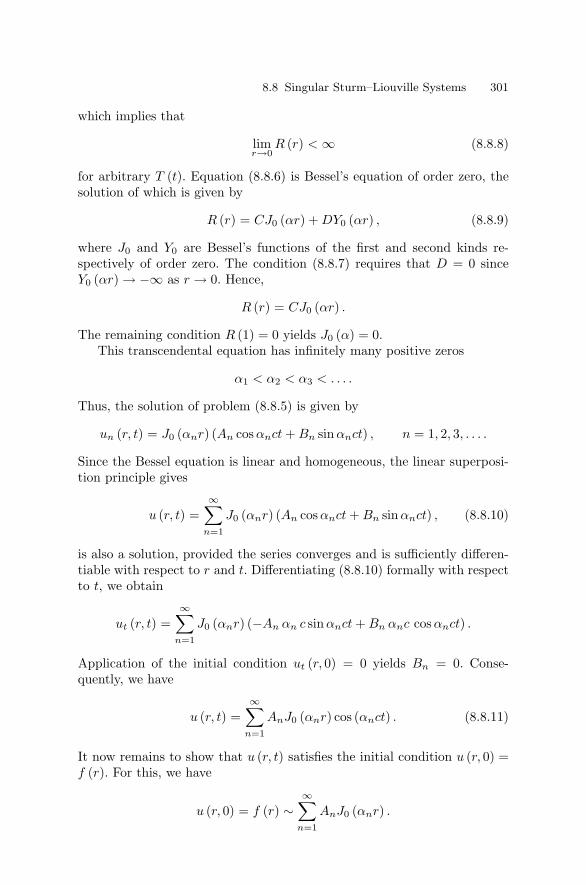
8.8 Singular Sturm–Liouville Systems 301
which implies that
limr→0
R (r) < ∞ (8.8.8)
for arbitrary T (t). Equation (8.8.6) is Bessel’s equation of order zero, thesolution of which is given by
R (r) = CJ0 (αr) + DY0 (αr) , (8.8.9)
where J0 and Y0 are Bessel’s functions of the first and second kinds re-spectively of order zero. The condition (8.8.7) requires that D = 0 sinceY0 (αr) → −∞ as r → 0. Hence,
R (r) = CJ0 (αr) .
The remaining condition R (1) = 0 yields J0 (α) = 0.This transcendental equation has infinitely many positive zeros
α1 < α2 < α3 < . . . .
Thus, the solution of problem (8.8.5) is given by
un (r, t) = J0 (αnr) (An cos αnct + Bn sin αnct) , n = 1, 2, 3, . . . .
Since the Bessel equation is linear and homogeneous, the linear superposi-tion principle gives
u (r, t) =∞∑
n=1
J0 (αnr) (An cos αnct + Bn sin αnct) , (8.8.10)
is also a solution, provided the series converges and is sufficiently differen-tiable with respect to r and t. Differentiating (8.8.10) formally with respectto t, we obtain
ut (r, t) =∞∑
n=1
J0 (αnr) (−An αn c sin αnct + Bn αnc cos αnct) .
Application of the initial condition ut (r, 0) = 0 yields Bn = 0. Conse-quently, we have
u (r, t) =∞∑
n=1
AnJ0 (αnr) cos (αnct) . (8.8.11)
It now remains to show that u (r, t) satisfies the initial condition u (r, 0) =f (r). For this, we have
u (r, 0) = f (r) ∼∞∑
n=1
AnJ0 (αnr) .

302 8 Eigenvalue Problems and Special Functions
If f (r) is piecewise smooth on [0, 1], then the eigenfunctions J0 (αnr) forma complete orthogonal system with respect to the weight function r overthe interval (0, 1). Hence, we can formally expand f (r) in terms of theeigenfunctions. Thus,
f (r) =∞∑
n=1
AnJ0 (αnr) , (8.8.12)
where the coefficient An is represented by
An =∫ 1
0rf (r) J0 (αnr) dr
/∫ 1
0r [J0 (αnr)]2 dr. (8.8.13)
The solution of the problem (8.8.5) is therefore given by (8.8.11) with thecoefficients An given by (8.8.13).
8.9 Legendre’s Equation and Legendre’s Function
The Legendre equation is(1 − x2) y′′ − 2xy′ + ν (ν + 1) y = 0, (8.9.1)
where ν is a real number. This equation arises in problems with sphericalsymmetry in mathematical physics. Its coefficients are analytic at x = 0.Thus, if we expand near the point x = 0, the coefficients are
p (x) = − 2x
1 − x2 = −2x
∞∑m=0
x2m =∞∑
m=0
(−2) x2m+1,
and
q (x) =ν (ν + 1)1 − x2 = ν (ν + 1)
∞∑m=0
x2m =∞∑
m=0
ν (ν + 1)x2m.
We see that these series converge for |x| < 1. Thus, the Legendre equationon |x| < 1 has convergent power series solution at x = 0.
Now to find the solution near the ordinary point x = 0, we assume
y (x) =∞∑
m=0
am xm.
Substituting y, y′, and y′′ in the Legendre equation, we obtain
(1 − x2) ∞∑
m=0
m (m − 1) am xm−2 − 2x
∞∑m=0
mam xm−1
+ν (ν + 1)∞∑
m=0
am xm = 0.

8.9 Legendre’s Equation and Legendre’s Function 303
Simplification gives
∞∑m=0
[(m + 1) (m + 2) am+2 + (ν − m) (ν + m + 1) am] xm = 0.
Therefore the coefficients in the power series must satisfy the recurrencerelation
am+2 = − (ν − m) (ν + m + 1)(m + 1) (m + 2)
am, m ≥ 0. (8.9.2)
This relation determines a2, a4, a6, . . . in terms of a0, and a3, a5, a7, . . . interms of a1. It can easily be verified that a2k and a2k+1 can be expressedin terms of a0 and a1 respectively as
a2k =(−1)k
ν (ν − 2) . . . (ν − 2k + 2) (ν + 1) (ν + 3) . . . (ν + 2k − 1)(2k)!
a0
and
a2k+1 =(−1)k (ν − 1) (ν − 3) . . . (ν − 2k + 1) (ν + 2) (ν + 4) . . . (ν + 2k)
(2k + 1)!a1.
Hence, the solution of the Legendre equation is
y (x) = a0
[1
+∞∑
k=1
(−1)kν (ν − 2) . . . (ν − 2k + 2) (ν + 1) (ν + 3) . . . (ν + 2k − 1) x2k
(2k)!
]
+a1
[x
+∞∑
k=1
(−1)k (ν − 1) (ν − 3) . . . (ν − 2k + 1) (ν + 2) (ν + 4) . . . (ν + 2k) x2k+1
(2k + 1)!
]= a0φν (x) + a1ψν (x) . (8.9.3)
It can easily be proved that the functions φν (x) and ψν (x) converge forx < 1 and are linearly independent.
Now consider the case in which ν = n, with n a nonnegative integer. Itis then evident from the recurrence relation (8.9.2) that, when m = n,
an+2 = an+4 = . . . = 0.
Consequently, when n is even, the series φn (x) terminates with xn, whereasthe series for ψn (x) does not terminate. When n is odd, it is the series forψn (x) which terminates with xn, while that for φn (x) does not terminate.

304 8 Eigenvalue Problems and Special Functions
In the first case (n even), φn (x) is a polynomial of degree n; the same istrue for ψn (x) in the second case (n odd).
Thus, for any nonnegative integer n, either φn (x) or ψn (x), but notboth, is a polynomial of degree n. Consequently, the general solution of theLegendre equation contains a polynomial solution Pn (x) and an infiniteseries solution Qn (x) for a nonnegative integer n. To find the polynomialsolution Pn (x), it is convenient to choose an so that Pn (1) = 1. Let thisan be
an =(2n)!
2n (n!)2. (8.9.4)
Rewriting the recurrence relation (8.9.2), we have
an−2 = − (n − 1) n
2 (2n − 1)an.
Substituting an from (8.9.4) into this relation, we obtain
an−2 = − (2n − 2)!2n (n − 1)! (n − 2)!
,
and
an−4 =(2n − 4)!
2n2! (n − 2)! (n − 4)!.
It follows by induction that
an−2k =(−1)k (2n − 2k)!
2nk! (n − k)! (n − 2k)!.
Hence, we may write Pn (x) in the form
Pn (x) =N∑
k=0
(−1)k (2n − 2k)!2nk! (n − k)! (n − 2k)!
xn−2k, (8.9.5)
where N = (n/2) when n is even, and N = (n − 1) /2 when n is odd. Thispolynomial Pn (x) is called the Legendre function of the first kind of ordern. It is also known as the Legendre polynomial of degree n.
The first few Legendre polynomials are
P0 (x) = 1,
P1 (x) = x,
P2 (x) =12(3x2 − 1
),
P3 (x) =12(5x3 − 3x
),
P4 (x) =18(35x4 − 30x2 + 3
).

8.9 Legendre’s Equation and Legendre’s Function 305
Figure 8.9.1 The first four Legendre’s polynomials.
These polynomials are plotted in Figure 8.9.1 for small values of x.Recall that for a given nonnegative integer n, only one of the two solu-
tions φn (x) and ψn (x) of Legendre’s equation is a polynomial, while theother in an infinite series. This infinite series, when appropriately normal-ized, is called the Legendre function of the second kind. It is defined for|x| < 1 by
Qn (x) =
⎧⎨⎩φn (1) ψn (x) for n even
−ψn (1) φn (x) for n odd. (8.9.6)
Thus, when n is a nonnegative integer, the general solution of the Legendreequation is given by
y (x) = c1Pn (x) + c2Qn (x) . (8.9.7)
The Legendre polynomial may also be expressed in the form
Pn (x) =1
2nn!dn
dxn
(x2 − 1
)n. (8.9.8)
This expression is known as the Rodriguez formula.Like Bessel’s functions, Legendre polynomials satisfy certain recurrence
relations. Some of the important relations are

306 8 Eigenvalue Problems and Special Functions
(n + 1)Pn+1 (x) − (2n + 1)xPn (x) + nPn−1 (x) = 0, n ≥ 1, (8.9.9)(x2 − 1
)P ′
n (x) = nxPn (x) − nPn−1 (x) , n ≥ 1, (8.9.10)nPn (x) + P ′
n−1 (x) − xP ′n (x) = 0, n ≥ 1, (8.9.11)
P ′n+1 (x) = xP ′
n (x) + (n + 1)Pn (x) , n ≥ 0. (8.9.12)
In addition,
P2n (−x) = P2n (x) , (8.9.13)P2n+1 (−x) = −P2n+1 (x) . (8.9.14)
These indicate that Pn (x) is an even function for even n, and an oddfunction for odd n.
It can easily be shown that the Legendre polynomials form a sequenceof orthogonal functions on the interval [−1, 1]. Thus, we have∫ 1
−1Pn (x) Pm (x) dx = 0, for n = m. (8.9.15)
The norm of the function Pn (x) is given by
‖Pn (x)‖2 =∫ 1
−1P 2
n (x) dx =2
2n + 1. (8.9.16)
Another important equation in mathematical physics, one which isclosely related to the Legendre equation (8.9.1), is Legendre’s associatedequation:
(1 − x2) y′′ − 2xy′ +
[n (n + 1) − m2
1 − x2
]y = 0, (8.9.17)
where m is an integer. Although this equation is independent of the alge-braic sign of the integer m, it is often convenient to have the solutions fornegative m differ somewhat from those for positive m.
We consider first the case for a nonnegative integer m. Introducing thechange of variable
y =(1 − x2)m/2
u, |x| < 1,
Legendre’s associated equation becomes(1 − x2)u′′ − 2 (m + 1)xu′ + (n − m) (n + m + 1)u = 0.
But this is the same as the equation obtained by differentiating the Legendreequation (8.9.1) m times. Thus, the general solution of (8.9.17) is given by
y (x) =(1 − x2)m/2 dmY (x)
dxm, (8.9.18)

8.9 Legendre’s Equation and Legendre’s Function 307
and
Y (x) = c1Pn (x) + c2Qn (x) (8.9.19)
is the general solution of (8.9.1). Hence, we have the linearly independentsolutions of (8.9.17), known as the associated Legendre functions of the firstand second kind, respectively given by
Pmn (x) =
(1 − x2)m/2 dmPn (x)
dxm, (8.9.20)
and
Qmn (x) =
(1 − x2)m/2 dmQn (x)
dxm. (8.9.21)
We observe that
P 0n (x) = Pn (x) , Q0
n (x) = Qn (x) ,
and that Pmn (x) vanishes for m > n.
The functions P−mn (x) and Q−m
n (x) are defined by
P−mn (x) = (−1)m (n − m)!
(n + m)!Pm
n (x) , m = 0, 1, 2, . . . , n, (8.9.22)
Q−mn (x) = (−1)m (n − m)!
(n + m)!Qm
n (x) , m = 0, 1, 2, . . . , n. (8.9.23)
The first few associated Legendre functions are
P 11 (x) =
(1 − x2) 1
2 ,
P 12 (x) = 3x
(1 − x2) 1
2 ,
P 22 (x) = 3
(1 − x2) .
The associated Legendre functions of the first kind also form a sequence oforthogonal functions in the interval [−1, 1]. Their orthogonality, as well astheir norm, is expressed by the equation∫ 1
−1Pm
n (x) Pmk (x) dx =
2 (n − m)!(2n + 1) (n + m)!
δnk. (8.9.24)
Note that (8.9.15) and (8.9.16) are special cases of (8.9.24), correspondingto the choice m = 0.
We finally observe that Pmn (x) is bounded everywhere in the interval
[−1, 1], whereas Qmn (x) is unbounded at the end points x = + 1.
Problems in which Legendre’s polynomials arise will be treated in Chap-ter 10.
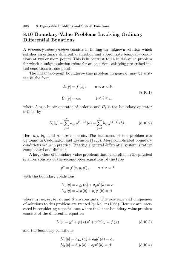
308 8 Eigenvalue Problems and Special Functions
8.10 Boundary-Value Problems Involving OrdinaryDifferential Equations
A boundary-value problem consists in finding an unknown solution whichsatisfies an ordinary differential equation and appropriate boundary condi-tions at two or more points. This is in contrast to an initial-value problemfor which a unique solution exists for an equation satisfying prescribed ini-tial conditions at one point.
The linear two-point boundary-value problem, in general, may be writ-ten in the form
L [y] = f (x) , a < x < b,
(8.10.1)Ui [y] = αi, 1 ≤ i ≤ n,
where L is a linear operator of order n and Ui is the boundary operatordefined by
Ui [y] =n∑
j=1
aij y(j−1) (a) +n∑
j=1
bij y(j−1) (b) . (8.10.2)
Here aij , bij , and αi are constants. The treatment of this problem canbe found in Coddington and Levinson (1955). More complicated boundaryconditions occur in practice. Treating a general differential system is rathercomplicated and difficult.
A large class of boundary-value problems that occur often in the physicalsciences consists of the second-order equations of the type
y′′ = f (x, y, y′) , a < x < b
with the boundary conditions
U1 [y] = a1y (a) + a2y′ (a) = α
U2 [y] = b1y (b) + b2y′ (b) = β
where a1, a2, b1, b2, α, and β are constants. The existence and uniquenessof solutions to this problem are treated by Keller (1968). Here we are inter-ested in considering a special case where the linear boundary-value problemconsists of the differential equation
L [y] = y′′ + p (x) y′ + q (x) y = f (x) (8.10.3)
and the boundary conditions
U1 [y] = a1y (a) + a2y′ (a) = α,
U2 [y] = b1y (b) + b2y′ (b) = β, (8.10.4)

8.10 Boundary-Value Problems Involving Ordinary Differential Equations 309
where the constants a1 and a2, and likewise b1 and b2, are not both zero,and α, and β are constants.
In general, a boundary-value problem may not possess a solution, andif it does, the solution may not be unique. We illustrate this with a simpleproblem.
Example 8.10.1. We first consider the boundary-value problem
y′′ + y = 1,
y (0) = 0, y(π
2
)= 0.
By the method of variation of parameters, we find a unique solution
y (x) = 1 − cos x − sin x.
We observe that the solution of the associated homogeneous boundary-valueproblem
y′′ + y = 0,
y (0) = 0, y(π
2
)= 0,
is trivial.Next we consider the boundary-value problem
y′′ + y = 1,
y (0) = 0, y (π) = 0.
The general solution is
y (x) = c1 cos x + c2 sin x + 1.
Applying the boundary conditions, we see that
y (0) = c1 + 1 = 0, y (π) = −c1 + 1 = 0.
This is not possible, and hence, the boundary-value problem has no solu-tion. However, if we consider its associated homogeneous boundary-valueproblem
y′′ + y = 0,
y (0) = 0, y (π) = 0,
we can easily determine that solutions exist and are given by
y (x) = c2 sin x,
where c2 is an arbitrary constant.

310 8 Eigenvalue Problems and Special Functions
This leads to the following alternative theorem:
Theorem 8.10.1. Let p (x), q (x), and f (x) be continuous on [a, b]. Theneither the boundary-value problem
L [y] = f
(8.10.5)U1 [y] = α, U2 [y] = β,
has a unique solution for any given constants α and β, or else the associatedhomogeneous boundary-value problem
L [y] = 0(8.10.6)
U1 [y] = 0, U2 [y] = 0,
has a nontrivial solution.
Proof of this theorem can be found in Myint-U (1978).
8.11 Green’s Functions for Ordinary DifferentialEquations
In the present section, we will introduce Green’s functions. Let us considerthe linear homogeneous ordinary differential equation of second order:
L [y] = −f (x) , a < x < b, (8.11.1)
where
L ≡ d
dr
[p (x)
d
dx
]+ q (x) ,
with the homogeneous boundary conditions
a1y (a) + a2y′ (a) = 0, (8.11.2)
b1y (b) + b2y′ (b) = 0, (8.11.3)
where the constants a1 and a2, and likewise b1 and b2, are not both zero.We shall assume that f and q are continuous and that p is continuouslydifferentiable and does not vanish in the interval [a, b].
According to the theory of ordinary differential equations, the generalsolution of (8.11.1) is given by
y (x) = A y1 (x) + B y2 (x) + yp (x) (8.11.4)

8.11 Green’s Functions for Ordinary Differential Equations 311
where A and B are arbitrary constants, y1 = y1 (x) and y2 = y2 (x) are twolinearly independent solutions of the corresponding homogeneous equationL [y] = 0, and yp (x) is a particular integral of (8.11.1).
Using the method of variation of parameters, the particular integral willbe sought by replacing the constants A and B by arbitrary functions of x,u1 (x) and u2 (x), to get
yp (x) = u1 (x) y1 (x) + u2 (x) y2 (x) . (8.11.5)
These arbitrary functions are to be determined so that (8.11.5) satisfiesequation (8.11.1). The substitution of the above trial form for yp (x) into(8.11.1) imposes one condition that (8.11.5) must satisfy. However, there aretwo arbitrary functions, and hence, two conditions are needed to determinethem. If follows that another condition is available in solving the problem.
The first task is to substitute the trial solution into equation (8.11.1).Differentiating yp (x), we obtain
y′p = u1y
′1 + u2y
′2 + u′
1y1 + u′2y2.
It is convenient to set the second condition noted above to require that
u′1y1 + u′
2y2 = 0, (8.11.6)
leaving
y′p = u1y
′1 + u2y
′2. (8.11.7)
A second differentiation of yp gives
y′′p = u1y
′′1 + u2y
′′2 + u′
1y′1 + u′
2y′2.
Putting these results into equation (8.11.1) and grouping yields
u1 [p (x) y′′1 + p′y′
1 + qy1] + u2 [p (x) y′′2 + p′y′
2 + qy2]+p (x) u′
1y′1 + u′
2y′2 = −f (x) .
Since y1 (x) and y2 (x) are solutions of the homogeneous equations, boththe square brackets in the above expression vanish. The result is that
u′1y
′1 + u′
2y′2 = −f (x)
p (x). (8.11.8)
Thus, two equations ((8.11.6) and (8.11.8)) determine u1 (x) and u2 (x).Solving these equations algebraically for u′
1 and u′2 produces
u′1 (x) =
f (x) y2 (x)p (x) W (x)
, u′2 (x) = −f (x) y1 (x)
p (x) W (x),

312 8 Eigenvalue Problems and Special Functions
where W (x) = (y1y′2 − y2y
′1) is the non-zero Wronskian of the solutions y1
and y2. Integration of these results yields
u1 (x) = +∫
f (x) y2 (x) dx
p (x) W (x), u2 (x) = −
∫f (x) y1 (x) dx
p (x) W (x).
The substitution of these results into (8.11.5) gives the solution in (a, b)
yp (x) = y1 (x)∫ x
b
f (ξ) y2 (ξ)p (ξ) W (ξ)
dξ − y2 (x)∫ x
a
f (ξ) y1 (ξ)p (ξ) W (ξ)
dξ
= −∫ x
a
y2 (x) y1 (ξ)p (ξ) W (ξ)
f (ξ) dξ −∫ b
x
y1 (x) y2 (ξ)p (ξ) W (ξ)
f (ξ) dξ. (8.11.9)
This form suggests the definition
G (x, ξ) =
⎧⎪⎨⎪⎩−y2(x)y1(ξ)
p(ξ)W (ξ) , a ≤ ξ < x,
−y1(x)y2(ξ)p(ξ)W (ξ) , x < ξ ≤ b.
(8.11.10)
This is called Green’s function. Thus, the solution becomes
yp (x) =∫ b
a
G (x, ξ) f (ξ) dξ (8.11.11)
provided G (x, ξ) is continuous and f (ξ) is at least piecewise continuous in(a, b). The existence of Green’s function is evident from equations (8.11.10)provided W (ξ) = 0.
In order to obtain a deeper insight into the role of Green’s function,certain properties are important to note. These are
(i) G (x, ξ) is continuous at x = ξ, and consequently, throughout the inter-val (a, b). This follows from the fact that G (x, ξ) is constructed fromthe solutions of the homogeneous equation which are continuous in theintervals a ≤ ξ < x and x < ξ ≤ b, W (ξ) = 0.
(ii) Its first and second derivatives are continuous for all x = ξ in a ≤ x,ξ ≤ b.
(iii) G (x, ξ) is symmetric in x and ξ, that is, if x and ξ are interchangedin (8.11.10), the definition is not changed.
(iv) The first derivative of G (x, ξ) has a finite discontinuity at x = ξ
limx→ξ+
(∂G
∂x
)− lim
x→ξ−
(∂G
∂x
)= − 1
p (ξ). (8.11.12)
(v) G (x, ξ) is a solution of the homogeneous equation throughout the inter-val except at x = ξ. This point can be pressed further by substitutionof (8.11.11) and (8.11.1), note that yp (x) is a solution of (8.11.1). Thisleads to

8.11 Green’s Functions for Ordinary Differential Equations 313∫ b
a
[d
dx
p (x)
dG (x, ξ)dx
+ q (x) G (x, ξ)
]f (ξ) dξ = −f (x) ,
where the quantity in the square bracket is zero except at x = ξ. Iffollows that, in order for this result to hold,
d
dx
[p (x)
dG (x, ξ)dx
]+ q (x) G (x, ξ) = −δ (ξ − x) , (8.11.13)
where δ (ξ − x) is the Dirac function which has the following properties:
δ (ξ − x) = 0, except at x = ξ,∫ b
a
δ (ξ − x) dξ = 1, a < x < b.
For any continuous function f (ξ) in (a, b) and for a ≤ x ≤ b,∫ b
a
f (ξ) δ (ξ − x) dξ = f (x) .
(vi) For fixed ξ, G (x, ξ) satisfies the given boundary conditions (8.11.2)–(8.11.3).Differentiating (8.11.11) with respect to x by Leibniz’s rule, we obtain
y′p (x) =
∫ b
a
G′ (x, ξ) f (ξ) dξ + G (x, x−) f (x)
+∫ b
a
G′ (x, ξ) f (ξ) dξ − G (x, x+) f (x)
=∫ b
a
G′ (x, ξ) f (ξ) dξ,
since G (x, ξ) is continuous in ξ, that is, G (x, x−) = G (x, x+).Because G (x, ξ) satisfies the boundary conditions, it follows that
a1yp (a) + a2y′p (a) =
∫ b
a
[a1G (a, ξ) + a2G′ (a, ξ)] f (ξ) dξ = 0.
Similarly,
b1yp (b) + b2y′p (b) = 0.
The result embodied in equation (8.11.13) permits a meaningful physi-cal interpretation of the role of Green’s function. If we assume that thedifferential equation (8.11.1) represents a vibrating mechanical systemdriven by a uniformly distributed force −f (x) in the interval (a, b),where the system is defined, then G (x, ξ) governed by (8.11.13) repre-sents the displacement of the system at a point x resulting from a unit

314 8 Eigenvalue Problems and Special Functions
impulse of force at x = ξ. The displacement at the point x due to uni-formly distributed force f (ξ) per unit length over an elementary interval(ξ, ξ + dξ) is given by f (ξ) G (x, ξ) dξ. Finally, the total displacementof the system at the point x results from superposition (addition) ofthese contributions so that the total solution over the entire interval(a, b) is given by (8.11.1), that is,
yp (x) =∫ b
a
G (x, ξ) f (ξ) dξ.
Combining all above results, we state the fundamental theorem forGreen’s function:
Theorem 8.11.1. If f (x) is continuous on [a, b], then the function
y (x) =∫ b
a
G (x, ξ) f (ξ) dξ
is a solution of the boundary-value problem
L [y] = −f (x) ,
a1y (a) + a2y′ (a) = 0, b1 (b) + b2y
′ (b) = 0.
Example 8.11.1. Consider the problem
y′′ = −x, y (0) = 0, y (1) = 0. (8.11.14)
For a fixed value of ξ, Green’s function G (x, ξ) satisfies the associatedhomogeneous equation
G′′ = 0
in 0 < x < ξ, ξ < x < 1, and the boundary conditions
G (0, ξ) = 0, G (1, ξ) = 0.
In addition, it satisfies
dG
dx(x, ξ)
∣∣∣∣x=ξ+
x=ξ−= − 1
p (ξ).
Now choose G (x, ξ) such that
G (x, ξ) =
⎧⎨⎩G1 (x, ξ) = (1 − ξ) x, for 0 ≤ x ≤ ξ
G2 (x, ξ) = (1 − x) ξ, for ξ ≤ x ≤ 1.
It can be seen that G′′ = 0 over the intervals 0 < x < ξ, ξ < x < 1. Also

8.12 Construction of Green’s Functions 315
G1 (0, ξ) = 0, G2 (1, ξ) = 0.
Moreover,
G′2 (x, ξ) − G′
1 (x, ξ) = −ξ − (1 − ξ) = −1
which is the value of the jump −1/p (ξ), because in this case p = 1. Hence,by Theorem 8.11.1, keeping in mind that ξ is the variable in G (x, ξ), thesolution of (8.11.14) is
y (x) =∫ x
0G (x, ξ) f (ξ) dξ +
∫ 1
x
G (x, ξ) f (ξ) dξ
=∫ x
0(1 − x) ξ2dξ +
∫ 1
x
x (1 − ξ) ξdξ =x
6(1 − x2) .
8.12 Construction of Green’s Functions
In the above example, we see that the solution was obtained immediately assoon as Green’s function was obtained properly. Thus, the real problem isnot that of finding the solution but that of determining Green’s function forthe problem. We will now show by construction that there exists a Green’sfunction for L [y] satisfying the prescribed boundary conditions.
We first assume that the associated homogeneous equation satisfying theconditions (8.11.2) and (8.11.3) has the trivial solution only, as in Example8.11.1. We construct the solution y1 (x) of the equation
L [y] = 0
satisfying a1y (a) + a2y′ (a) = 0. We see that c1y1 (x) is the most general
such solution, where c1 is an arbitrary constant.In a similar manner, we let c2y2 (x), with c2 is an arbitrary constant,
be the most general solution of
L [y] = 0
satisfying b1y (b) + b2y′ (b) = 0. Thus, y1 and y2 exist in the interval (a, b)
and are linearly independent. For, if they were linearly dependent, theny1 = c y2, which shows that y1 would satisfy both the boundary conditionsat x = a and x = b. This contradicts our assumption about the trivialsolution. Consequently, Green’s function can take the form
G (x, ξ) =
⎧⎨⎩c1 (ξ) y1 (x) , for x < ξ
c2 (ξ) y2 (x) , for x > ξ. (8.12.1)
Since G (x, ξ) is continuous at x = ξ, we have

316 8 Eigenvalue Problems and Special Functions
c2 (ξ) y2 (ξ) − c1 (ξ) y1 (ξ) = 0. (8.12.2)
The discontinuity in the derivative of G at the point requires that
dG
dx(x, ξ)
∣∣∣∣x=ξ+
x=ξ−= c2 (ξ) y′
2 (ξ) − c1 (ξ) y′1 (ξ) = − 1
p (ξ). (8.12.3)
Solving equations (8.12.2) and (8.12.3) for c1 and c2, we find
c1 (ξ) =−y2 (ξ)
p (ξ) W (y1, y2; ξ), c2 (ξ) =
−y1 (ξ)p (ξ) W (y1, y2; ξ)
, (8.12.4)
where W (y1, y2; ξ) is the Wronskian given by W (y1, y2; ξ) = y1 (ξ) y′2 (ξ) −
y2 (ξ) y′1 (ξ). Since the two solutions are linearly independent, the Wronskian
differs from zero.From Theorem 8.2.6, with λ = 0, we have
p W = constant = C. (8.12.5)
Hence, Green’s function is given by
G (x, ξ) =
⎧⎨⎩−y1 (x) y2 (ξ) /C, for x ≤ ξ
−y2 (x) y1 (ξ) /C, for x ≥ ξ.(8.12.6)
Thus, we state the following theorem:
Theorem 8.12.1. If the associated homogeneous boundary-value problemof (8.11.1)–(8.11.3) has the trivial solution only, then Green’s function ex-ists and is unique.
Proof. The proof for uniqueness of Green’s function is left as an exercisefor the reader.
Example 8.12.1. Consider the problem
y′′ + y = −1, y (0) = 0, y(π
2
)= 0. (8.12.7)
The solution of L [y] = (dy′/dx) + y = 0 satisfying y (0) = 0 is
y1 (x) = sinx, 0 ≤ x < ξ
and the solution of L [y] = 0 satisfying y (π/2) = 0 is
y2 (x) = cos x, ξ < x ≤ π
2.
The Wronskian of y1 and y2 is then given by
W (ξ) = y1 (ξ) y′2 (ξ) − y2 (ξ) y′
1 (ξ) = −1.

8.13 The Schrodinger Equation and Linear Harmonic Oscillator 317
Since in this case p = 1, (8.12.6) becomes
G (x, ξ) =
⎧⎨⎩sin x cos ξ, for x ≤ ξ
cos x sin ξ, for x ≥ ξ.
Therefore, the solution of (8.12.7) is
y (x) =∫ x
0G (x, ξ) f (ξ) dξ +
∫ π/2
x
G (x, ξ) f (ξ) dξ
=∫ x
0cos x sin ξ dξ +
∫ π/2
x
sin x cos ξ dξ
= −1 + sin x + cos x.
It can be seen in the formula (8.12.6) that Green’s function is symmetricin x and ξ.
Example 8.12.2. Construct the Green’s function for the two-point boundary-value problem
y′′ (x) + ω2y = f (x) , y (a) = y (b) = 0.
This describes the forced oscillation of an elastic string with fixed ends atx = a and x = b.
It is easy to check that sin ωx and cosωx are two functions which satisfythe homogeneous equation y′′ + ω2y = 0. These are used to construct twofunctions y1 (x) and y2 (x) which satisfy the boundary conditions y1 (a) =y2 (b) = 0. Accordingly, y1 (x) = A sin ωx+B cos ωx and y2 (x) = C sin ωx+D cos ωx, and the resulting functions are
y1 (x) = sinω (x − a) , y2 (x) = sinω (x − b) .
The corresponding Wronskian is W = −ω sin ω (a − b). Substituting theseresults into (8.11.10) yields
G (x, ξ) =
⎧⎪⎨⎪⎩sin ω(ξ−a) sin ω(x−b)
−ω sin ω(a−b) , a ≤ ξ < x
sin ω(x−a) sin ω(ξ−b)−ω sin ω(a−b) , x ≤ ξ ≤ b
provided sinω (a − b) = 0.
8.13 The Schrodinger Equation and Linear HarmonicOscillator
The quantum mechanical motion of the harmonic oscillator is described bythe one-dimensional Schrodinger equation

318 8 Eigenvalue Problems and Special Functions
Hψ (x) = Eψ (x) , (8.13.1)
where the Hamiltonian H is given by
H = −(
2
2M
)d2
dx2 + V (x) , V (x) =12Mω2x2, (8.13.2)
and E is the energy, V (x) is the potential, h = 2π is the Planck con-stant, M is the mass of the particle, and ω is the classical frequency of theoscillator.
We solve equation (8.13.1) subject to the requirement that the solutionbe bounded as |x| → ∞. The solution of (8.13.1) is facilitated by the firstsolving the equation for large x. In terms of the constants
β =2ME
2 , α =Mω
> 0,
the equation (8.13.1) takes the form
d2ψ
dx2 +(β − α2x2)ψ = 0. (8.13.3)
For small β and large x, β − α2x2 ∼ −α2x2 so that the equation becomes
d2ψ
dx2 − α2x2ψ = 0.
As |x| → ∞, ψ (x) = xn exp(+ αx2
2
)satisfies (8.13.3) for a finite n so far
as leading terms(∼ −α2x2
)are concerned. The positive exponential fac-
tor is unacceptable because of the boundary conditions, so the asymptoticsolution ψ (x) = xn exp
(−αx2
2
)suggests the possibility of the exact solu-
tion in the form ψ (x) = v (x) exp(−αx2
2
)where v (x) is to be determined.
Substituting this result into (8.13.3), we obtain
d2v
dx2 − 2αxdv
dx+ (β − α) v = 0. (8.13.4)
In terms of a new independent variable ζ = x√
α, this equation reducesto the form
d2v
dζ2 − 2ζdv
dζ+
(β
α− 1
)v = 0. (8.13.5)
We seek a power series solution
v (ζ) =∞∑
n=0
anζn. (8.13.6)

8.13 The Schrodinger Equation and Linear Harmonic Oscillator 319
Substituting this series into equation (8.13.5) and equating the coefficientsof ζn to zero, we obtain the recurrence relation
an+2 =(2n + 1 − β/α)(n + 1) (n + 2)
an (8.13.7)
which gives
an+2
an∼ 2
nas n → ∞. (8.13.8)
This ratio is the same as that of the series for ζn exp(ζ2
) (∼ xneαx2
)with
finite n. This leads to the fact that ψ (x) = v (x) e−αx2/2 ∼ xneαx2/2 whichdoes not satisfy the basic requirement for |x| → ∞. This unacceptableresult can only be avoided if n is an integer and the series terminates sothat it becomes a polynomial of degree n. This means that an+2 = 0 butan = 0 so that
2n + 1 − β
α= 0, (8.13.9)
or
β
α= (2n + 1) .
Substituting the values for α and β, it turns out that
E ≡ En =(
n +12
)ω, n = 0, 1, 2, . . . . (8.13.10)
This represents a discrete set of energies. Thus, in quantum mechanics,a stationary state of the harmonic oscillator can assume only one of thevalues from the set En. The energy is thus quantized, and forms a discretespectrum. According to the classical theory, the energy forms a continuousspectrum, that is, all non-negative numbers are allowed for the energy of aharmonic oscillator. This shows a remarkable contrast between the resultsof the classical and quantum theory.
The number n which characterizes the energy eigenvalues and eigen-functions is called the quantum number. The value of n = 0 corresponds tothe minimum value of the quantum number with the energy
E0 =12
ω. (8.13.11)
This is called the lowest (or ground) state energy which never vanishes asthe lowest possible classical energy would. E0 is proportional to , repre-senting a quantum phenomenon. The discrete energy spectrum is in perfectagreement with the quantization rules of the quantum theory.

320 8 Eigenvalue Problems and Special Functions
To determine the eigenfunctions for the harmonic oscillator associatedwith the eigenvalues En, we obtain the solution of equation (8.13.5) whichhas the form
d2v
dζ2 − 2ζdv
dζ+ 2nv = 0. (8.13.12)
This is a well-known differential equation for the Hermite polynomialsHn (ζ) of degree n. Thus, the complete eigenfunctions can be expressedin terms of Hn (ζ) as
ψn (x) = AnHn
(x√
α)exp
(−αx2
2
), (8.13.13)
where An are arbitrary constants.The Hermite polynomials Hn (x) are usually defined by
Hn (x) = (−1)nex2
Dn(e−x2
), D ≡ d
dx. (8.13.14)
They form an orthogonal system in (−∞,∞) with the weight functionexp
(−x2).
The orthogonal relation for these polynomials is
∫ ∞
−∞e−x2
Hm (x) Hn (x) dx =
⎧⎨⎩0, n = m
2nn!√
π, n = m.
The Hermite polynomials Hn (x) for n = 0, 1, 2, 3, 4 are
H0 (x) = 1H1 (x) = 2x
H2 (x) = −2 + 4x2
H3 (x) = −12x + 8x3
H4 (x) = 12 − 48x2 + 16x4.
Finally, the eigenfunctions ψn of the linear harmonic oscillator for the quan-tum number n = 0, 1, 2, 3 are given in Figure 8.13.1.

8.14 Exercises 321
Figure 8.13.1 Eigenfunctions ψn for n = 0, 1, 2, 3.
8.14 Exercises
1. Determine the eigenvalues and eigenfunctions of the following regularSturm–Liouville systems:
(a) y′′ + λy = 0,
y (0) = 0, y (π) = 0.
(b) y′′ + λy = 0,
y (0) = 0, y′ (1) = 0.
(c) y′′ + λy = 0,
y′ (0) = 0, y′ (π) = 0.
(d) y′′ + λy = 0,
y (1) = 0, y (0) + y′ (0) = 0.

322 8 Eigenvalue Problems and Special Functions
2. Find the eigenvalues and eigenfunctions of the following periodic Sturm–Liouville systems:
(a) y′′ + λy = 0,
y (−1) = y (−1) , y′ (−1) = y′ (1).
(b) y′′ + λy = 0,
y (0) = y (2π) , y′ (0) = y′ (2π).
(c) y′′ + λy = 0,
y (0) = y (π) , y′ (0) = y′ (π).
3. Obtain the eigenvalues and eigenfunctions of the following Sturm–Liouville systems:
(a) y′′ + y′ + (1 + λ) y = 0,
y (0) = 0, y (1) = 0.
(b) y′′ + 2y′ + (1 − λ) y = 0,
y (0) = 0, y′ (1) = 0.
(c) y′′ − 3y′ + 3 (1 + λ) y = 0,
y′ (0) = 0, y′ (π) = 0.
4. Find the eigenvalues and eigenfunctions of the following regular Sturm–Liouville systems:
(a) x2y′′ + 3xy′ + λy = 0, 1 ≤ x ≤ e,
y (1) = 0, y (e) = 0.
(b) ddx
[(2 + x)2 y′
]+ λy = 0, −1 ≤ x ≤ 1,
y (−1) = 0, y (1) = 0.
(c) (1 + x)2 y′′ + 2 (1 + x) y′ + 3λy = 0, 0 ≤ x ≤ 1,
y (0) = 0, y (1) = 0.

8.14 Exercises 323
5. Determine all eigenvalues and eigenfunctions of the Sturm–Liouvillesystems:
(a) x2y′′ + xy′ + λy = 0,
y (1) = 0, y, y′ are bounded at x = 0.
(b) y′′ + λy = 0,
y (0) = 0, y, y′ are bounded at infinity.
6. Expand the function
f (x) = sinx, 0 ≤ x ≤ π
in terms of the eigenfunctions of the Sturm–Liouville problem
y′′ + λy = 0,
y (0) = 0, y (π) + y′ (π) = 0.
7. Find the expansion of
f (x) = x, 0 ≤ x ≤ π
in a series of eigenfunctions of the Sturm–Liouville system
y′′ + λy = 0,
y′ (0) = 0, y′ (π) = 0.
8. Transform each of the following equations into the equivalent self-adjoint form:(a) The Laguerre equation
xy′′ + (1 − x) y′ + ny = 0, n = 0, 1, 2, . . . .
(b) The Hermite equation
y′′ − 2xy′ + 2ny = 0, n = 0, 1, 2, . . . .
(c) The Tchebycheff equation(1 − x2) y′′ − xy′ + n2y = 0, n = 0, 1, 2, . . . .
9. If q (x) and s (x) are continuous and p (x) is twice continuously differ-entiable in [a, b], show that the solutions of the fourth-order Sturm–Liouville system

324 8 Eigenvalue Problems and Special Functions
[p (x) y′′]′′ + [q (x) + λs (x)] y = 0,
[a1y + a2 (py′′)′]
x=a= 0,
[b1y + b2 (py′′)′]
x=b= 0,
[c1y′ + c2 (py′′)]x=a = 0, [d1y
′ + d2 (py′′)]x=b = 0,
where a21 + a2
2 = 0, b21 + b2
2 = 0, c21 + c2
2 = 0, d21 + d2
2 = 0,are orthogonal with respect to s (x) in [a, b].
10. If the eigenfunctions of the problem
1r
d
dr(ry′) + λy = 0, 0 < r < a,
c1y (a) + c2y′ (a) = 0,
limr→0+
y (r) < ∞,
satisfy
limr→0+
ry′ (r) = 0,
show that all the eigenvalues are real for real c1 and c2.
11. Find the Green’s function for each of the following problems:
(a) L [y] = y′′ = 0,
y (0) = 0, y′ (1) = 0.
(b) L [y] =(1 − x2
)y′′ − 2xy′ = 0,
y (0) = 0, y′ (1) = 0.
(c) L [y] = y′′ + a2y = 0, a = constant,
y (0) = 0, y (1) = 0.
12. Determine the solution of each of the following boundary-value prob-lems:
(a) y′′ + y = 1,
y (0) = 0, y (1) = 0.
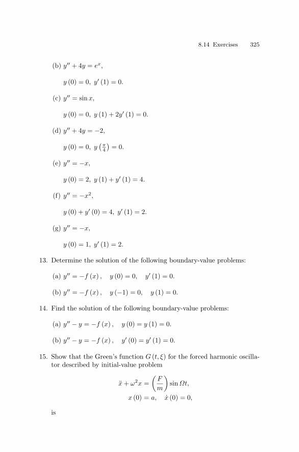
8.14 Exercises 325
(b) y′′ + 4y = ex,
y (0) = 0, y′ (1) = 0.
(c) y′′ = sinx,
y (0) = 0, y (1) + 2y′ (1) = 0.
(d) y′′ + 4y = −2,
y (0) = 0, y(
π4
)= 0.
(e) y′′ = −x,
y (0) = 2, y (1) + y′ (1) = 4.
(f) y′′ = −x2,
y (0) + y′ (0) = 4, y′ (1) = 2.
(g) y′′ = −x,
y (0) = 1, y′ (1) = 2.
13. Determine the solution of the following boundary-value problems:
(a) y′′ = −f (x) , y (0) = 0, y′ (1) = 0.
(b) y′′ = −f (x) , y (−1) = 0, y (1) = 0.
14. Find the solution of the following boundary-value problems:
(a) y′′ − y = −f (x) , y (0) = y (1) = 0.
(b) y′′ − y = −f (x) , y′ (0) = y′ (1) = 0.
15. Show that the Green’s function G (t, ξ) for the forced harmonic oscilla-tor described by initial-value problem
x + ω2x =(
F
m
)sin Ωt,
x (0) = a, x (0) = 0,
is
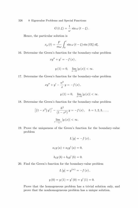
326 8 Eigenvalue Problems and Special Functions
G (t, ξ) =1ω
sin ω (t − ξ) .
Hence, the particular solution is
xp (t) =F
mω
∫ t
0sin ω (t − ξ) sin (Ωξ) dξ.
16. Determine the Green’s function for the boundary-value problem
xy′′ + y′ = −f (x) ,
y (1) = 0, limx→0
|y (x)| < ∞.
17. Determine the Green’s function for the boundary-value problem
xy′′ + y′ − n2
xy = −f (x) ,
y (1) = 0, limx→0
|y (x)| < ∞.
18. Determine the Green’s function for the boundary-value problem
[(1 − x2) y′]′ − h2
(1 − x2)y = −f (x) , h = 1, 2, 3, . . . ,
limr→+ 1
|y (x)| < ∞.
19. Prove the uniqueness of the Green’s function for the boundary-valueproblem
L [y] = −f (x) ,
a1y (a) + a2y′ (a) = 0,
b1y (b) + b2y′ (b) = 0.
20. Find the Green’s function for the boundary-value problem
L [y] = y(iv) = −f (x) ,
y (0) = y (1) = y′ (0) = y′ (1) = 0.
Prove that the homogeneous problem has a trivial solution only, andprove that the nonhomogeneous problem has a unique solution.

8.14 Exercises 327
21. Determine the Green’s function for the boundary-value problem
y′′ = −f (x) , y (−1) = y (1) , y′ (−1) = y′ (1) .
22. Consider the nonself-adjoint boundary-value problem
L [y] = y′′ + 3y′ + 2y = −f (x) ,
2 y (0) − y (1) = 0, y′ (1) = 2.
By direct integration of GL [y] from 0 to 1, show that
y (x) = −2 G (1, x) −∫ 1
0G (x, ξ) f (ξ) dξ
is the solution of the boundary-value problem, if G satisfies the system
Gξξ − 3Gξ + 2G = 0, ξ = x,
G (0, x) = 0,6 G (1, x) − 2 Gξ (1, x) + Gξ (0, x) = 0.
Find the Green’s function G (x, ξ).
23. Show that
dG (x, ξ)dx
∣∣∣∣ξ=x+
ξ=x−=
1p (x)
is equivalent to
dG (x, ξ)dx
∣∣∣∣x=ξ+
x=ξ−= − 1
p (ξ).
24. (a) Apply the Prufer transformation
R2 = y2 + p2 (y′)2 , θ = tan−1(
y
py′
)to transform the Sturm–Liouville equation (8.1.3) into the first ordernonlinear equation in the form
dR
dx=
12r
(1p
− q − λr
)sin 2θ,
dθ
dx= (q + λr) sin2 θ +
1p
cos2 θ,
where a < x < b.(b) Draw the direction field
(dθdx
)in the (θ, x) plane with p = x, q = − 1
xand r = x. Hence draw the solution curves of the θ-equation for differentλ with data θ (a) = α and θ (b) is arbitrary.

9
Boundary-Value Problems and Applications
“The enormous usefulness of mathematics in the natural sciences is some-thing bordering on the mysterious and there is no rational explanation forit. It is not at all natural that “laws of nature” exist, much less that man isable to discover them. The miracle of the appropriateness of the languageof mathematics for the formulation of the laws of physics is a wonderful giftwhich we neither understand nor deserve.”
Eugene Wigner
9.1 Boundary-Value Problems
In the preceding chapters, we have treated the initial-value and initialboundary-value problems. In this chapter, we shall be concerned withboundary-value problems. Mathematically, a boundary-value problem isfinding a function which satisfies a given partial differential equation andparticular boundary conditions. Physically speaking, the problem is inde-pendent of time, involving only space coordinates. Just as initial-value prob-lems are associated with hyperbolic partial differential equations, boundary-value problems are associated with partial differential equations of elliptictype. In marked contrast to initial-value problems, boundary-value prob-lems are considerably more difficult to solve. This is due to the physicalrequirement that solutions must hold in the large unlike the case of initial-value problems, where solutions in the small, say over a short interval oftime, may still be of physical interest.
The second-order partial differential equation of the elliptic type in nindependent variables x1, x2, . . ., xn is of the form
2u = F (x1, x2 . . . , xn, ux1 , ux2 , . . . , uxn) , (9.1.1)
where

330 9 Boundary-Value Problems and Applications
2u =n∑
i=1
uxixi.
Some well-known elliptic equations includeA. Laplace equation
2u = 0. (9.1.2)
B. Poisson equation
2u = g (x) , (9.1.3)
where
g (x) = g (x1, x2, . . . , xn) .
C. Helmholtz equation
2u + λu = 0, (9.1.4)
where λ is a positive constantD. Schrodinger equation (time independent)
2u + [λ − q (x)] u = 0. (9.1.5)
We shall not attempt to treat general elliptic partial differential equa-tions. Instead, we shall begin by presenting the simplest boundary-valueproblems for the Laplace equation in two dimensions.
We first define a harmonic function. A function is said to be harmonicin a domain D if it satisfies the Laplace equation and if it and its first twoderivatives are continuous in D.
We may note here that, since the Laplace equation is linear and homo-geneous, a linear combination of harmonic functions is harmonic.
1. The First Boundary-Value Problem
The Dirichlet Problem: Find a function u(x, y), harmonic in D, which sat-isfies
u = f (s) on B, (9.1.6)
where f (s) is a prescribed continuous function on the boundary B of thedomain D. D is the interior of a simple closed piecewise smooth curve B.
We may physically interpret the solution u of the Dirichlet problem asthe steady-state temperature distribution in a body containing no sources orsinks of heat, with the temperature prescribed at all points on the boundary.
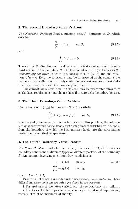
9.1 Boundary-Value Problems 331
2. The Second Boundary-Value Problem
The Neumann Problem: Find a function u (x, y), harmonic in D, whichsatisfies
∂u
∂n= f (s) on B, (9.1.7)
with ∫B
f (s) ds = 0. (9.1.8)
The symbol ∂u/∂n denotes the directional derivative of u along the out-ward normal to the boundary B. The last condition (9.1.8) is known as thecompatibility condition, since it is a consequence of (9.1.7) and the equa-tion 2u = 0. Here the solution u may be interpreted as the steady-statetemperature distribution in a body containing no heat sources or heat sinkswhen the heat flux across the boundary is prescribed.
The compatibility condition, in this case, may be interpreted physicallyas the heat requirement that the net heat flux across the boundary be zero.
3. The Third Boundary-Value Problem
Find a function u (x, y) harmonic in D which satisfies
∂u
∂n+ h (s) u = f (s) on B, (9.1.9)
where h and f are given continuous functions. In this problem, the solutionu may be interpreted as the steady-state temperature distribution in a body,from the boundary of which the heat radiates freely into the surroundingmedium of prescribed temperature.
4. The Fourth Boundary-Value Problem
The Robin Problem: Find a function u (x, y), harmonic in D, which satisfiesboundary conditions of different types on different portions of the boundaryB. An example involving such boundary conditions is
u = f1 (s) on B1, (9.1.10)∂u
∂n= f2 (s) on B2,
where B = B1 ∪ B2.Problems 1 through 4 are called interior boundary-value problems. These
differ from exterior boundary-value problems in two respects:i. For problems of the latter variety, part of the boundary is at infinity.ii. Solutions of exterior problems must satisfy an additional requirement,
namely, that of boundedness at infinity.

332 9 Boundary-Value Problems and Applications
9.2 Maximum and Minimum Principles
Before we prove the uniqueness and continuity theorems for the interiorDirichlet problem for the two-dimensional Laplace equation, we first provethe maximum and minimum principles.
Theorem 9.2.1. (The Maximum Principle) Suppose that u (x, y) isharmonic in a bounded domain D and continuous in D = D ∪ B. Then uattains its maximum on the boundary B of D.
Physically, we may interpret this as meaning that the temperature of abody which was neither a source nor a sink of heat acquires its largest (andsmallest) values on the surface of the body, and the electrostatic potential ina region which does not contain any free charge attains its maximum (andminimum) values on the boundary of the region.
Proof. Let the maximum of u on B be M . Let us now suppose thatthe maximum of u in D is not attained at any point of B. Then it mustbe attained at some point P0 (x0, y0) in D. If M0 = u (x0, y0) denotes themaximum of u in D, then M0 must also be the maximum of u in D.
Consider the function
v (x, y) = u (x, y) +M0 − M
4R2
[(x − x0)
2 + (y − y0)2], (9.2.1)
where the point P (x, y) is in D and where R is the radius of a circlecontaining D. Note that
v (x0, y0) = u (x0, y0) = M0.
We have v (x, y) ≤ M + (M0 − M) /2 = 12 (M + M0) < M0 on B. Thus,
v (x, y) like u (x, y) must attain its maximum at a point in D. It followsfrom the definition of v that
vxx + vyy = uxx + uyy +(M0 − M)
R2 =(M0 − M)
R2 > 0. (9.2.2)
But for v to be a maximum in D,
vxx ≤ 0, vyy ≤ 0.
Thus,
vxx + vyy ≤ 0
which contradicts equation (9.2.2). Hence, the maximum of u must be at-tained on B.
Theorem 9.2.2. (The Minimum Principle) If u (x, y) is harmonic ina bounded domain D and continuous in D = D ∪ B, then u attains itsminimum on the boundary B of D.

9.3 Uniqueness and Continuity Theorems 333
Proof. The proof follows directly by applying the preceding theorem tothe harmonic function −u (x, y).
As a result of the above theorems, we see that u =constant which is evi-dently harmonic attains the same value in the domain D as on the boundaryB.
9.3 Uniqueness and Continuity Theorems
Theorem 9.3.1. (Uniqueness Theorem) The solution of the Dirichletproblem, if it exists, is unique.
Proof. Let u1 (x, y) and u2 (x, y) be two solutions of the Dirichlet prob-lem. Then u1 and u2 satisfy
2u1 = 0, 2u2 = 0 in D,
u1 = f, u2 = f on B.
Since u1 and u2 are harmonic in D, (u1 − u2) is also harmonic in D.But
u1 − u2 = 0 on B.
The maximum-minimum principle gives
u1 − u2 = 0
at all interior points of D. Thus, we have
u1 = u2.
Therefore, the solution is unique.
Theorem 9.3.2. (Continuity Theorem) The solution of the Dirichletproblem depends continuously on the boundary data.
Proof. Let u1 and u2 be the solutions of
2u1 = 0 in D,
u1 = f1 on B,
and
2u2 = 0 in D,
u2 = f2 on B.
If v = u1 − u2, then v satisfies

334 9 Boundary-Value Problems and Applications
2v = 0 in D,
v = f1 − f2 on B.
By maximum and minimum principles, f1 − f2 attains the maximumand minimum of v on B . Thus, if |f1 − f2| < ε, then
−ε < vmin ≤ vmax < ε on B.
Thus, at any interior point in D , we have
−ε < vmin ≤ v ≤ vmax < ε.
Therefore, |v| < ε in D. Hence,
|u1 − u2| < ε.
Theorem 9.3.3. Let un be a sequence of functions harmonic in D andcontinuous in D. Let fi be the values of ui on B. If a sequence un con-verges uniformly on B, then it converges uniformly in D.
Proof. By hypothesis, fn converges uniformly on B. Thus, for ε > 0,there exists an integer N such that everywhere on B
|fn − fm| < ε for n, m > N.
It follows from the continuity theorem that for all n, m > N
|un − um| < ε
in D, and hence, the theorem is proved.
9.4 Dirichlet Problem for a Circle
1. Interior Problem
We shall now establish the existence of the solution of the Dirichlet problemfor a circle.
The Dirichlet problem is
2u = urr +1r
ur +1r2 uθθ = 0, 0 ≤ r < a, 0 < θ ≤ 2π,(9.4.1)
u (a, θ) = f (θ) for all θ in [0, 2π] . (9.4.2)
By the method of separation of variables, we seek a solution in the form
u (r, θ) = R (r) Θ (θ) = 0.
Substitution of this in equation (9.4.1) yields

9.4 Dirichlet Problem for a Circle 335
r2 R′′
R+ r
R′
R= −Θ
′′
Θ= λ.
Hence,
r2R′′
+ rR′ − λR = 0, (9.4.3)
Θ′′
+ λΘ = 0. (9.4.4)
Because of the periodicity conditions Θ (0) = Θ (2π) and Θ′(0) =
Θ′(2π) which ensure that the function Θ is single-valued, the case λ < 0
does not yield an acceptable solution. When λ = 0, we have
u (r, θ) = (A + B log r) (Cθ + D) .
Since log r → −∞ as r → 0+ (note that r = 0 is a singular point ofequation (9.4.1)), B must vanish in order for u to be finite at r = 0. Cmust also vanish in order for u to be periodic with period 2π. Hence, thesolution for λ = 0 is u = constant. When λ > 0, the solution of equation(9.4.4) is
Θ (θ) = A cos√
λ θ + B sin√
λ θ.
The periodicity conditions imply√
λ = n for n = 1, 2, 3, . . . .
Equation (9.4.3) is the Euler equation and therefore, the general solutionis
R (r) = Crn + Dr−n.
Since r−n → ∞ as r → 0, D must vanish for u to be continuous atr = 0.
Thus, the solution is
u (r, 0) = Crn (A cos n θ + B sin n θ) for n = 1, 2, . . . .
Hence, the general solution of equation (9.4.1) may be written in theform
u (r, θ) =a0
2+
∞∑n=1
( r
a
)n
(an cos nθ + bn sin nθ) , (9.4.5)
where the constant term (a0/2) represents the solution for λ = 0, and an
and bn are constants. Letting ρ = r/a, we have
u (ρ, θ) =a0
2+
∞∑n=1
ρn (an cos nθ + bn sin nθ) . (9.4.6)

336 9 Boundary-Value Problems and Applications
Our next task is to show that u (r, θ) is harmonic in 0 ≤ r < a andcontinuous in 0 ≤ r ≤ a. We must also show that u satisfies the boundarycondition (9.4.2).
We assume that an and bn are the Fourier coefficients of f (θ), that is,
an =1π
∫ 2π
0f (θ) cos nθ dθ, n = 0, 1, 2, 3, . . . ,
(9.4.7)
bn =1π
∫ 2π
0f (θ) sin nθ dθ, n = 1, 2, 3, . . . .
Thus, from their very definitions, an and bn are bounded, that is, thereexists some number M > 0 such that
|a0| < M, |an| < M, |bn| < M, n = 1, 2, 3, . . . .
Thus, if we consider the sequence of functions un defined by
un (ρ, θ) = ρn (an cos nθ + bn sin nθ) , (9.4.8)
we see that
|un| < 2ρn0M, 0 ≤ ρ ≤ ρ0 < 1.
Hence, in any closed circular region, series (9.4.6) converges uniformly.Next, differentiate un with respect to r. Then, for 0 ≤ ρ ≤ ρ0 < 1,∣∣∣∣∂un
∂r
∣∣∣∣ =∣∣∣na
ρn−1 (an cos nθ + bn sin nθ)∣∣∣ < 2
(n
a
)ρn−10 M.
Thus, the series obtained by differentiating series (9.4.6) term by termwith respect to r converges uniformly. In a similar manner, we can provethat the series obtained by twice differentiating series (9.4.6) term by termwith respect to r and θ converge uniformly. Consequently,
2u = urr +1r
ur +1r2 uθθ
=∞∑
n=1
ρn−2
a2 (an cos nθ + bn sin nθ)[n (n − 1) + n − n2]
= 0, 0 ≤ ρ ≤ ρ0 < 1.
Since each term of series (9.4.6) is a harmonic function, and since theseries converges uniformly, u (r, θ) is harmonic at any interior point of theregion 0 ≤ ρ < 1. It now remains to show that u satisfies the boundarydata f (θ).
Substitution of the Fourier coefficients an and bn into equation (9.4.6)yields

9.4 Dirichlet Problem for a Circle 337
u (ρ, θ) =12π
∫ 2π
0f (θ) dθ +
1π
∞∑n=1
ρn
∫ 2π
0f (τ)
× (cos nτ cos nθ + sin nτ sin nθ) dτ
=12π
∫ 2π
0
[1 + 2
∞∑n=1
ρn cos n (θ − τ)
]f (τ) dτ. (9.4.9)
The interchange of summation and integration is permitted due to theuniform convergence of the series. For 0 ≤ ρ ≤ 1
1 + 2∞∑
n=1
[ρn cos n (θ − τ)] = 1 +∞∑
n=1
[ρnein(θ−τ) + ρne−in(θ−τ)
]= 1 +
ρ ei(θ−τ)
1 − ρ ei(θ−τ) +ρ e−i(θ−τ)
1 − ρ e−i(θ−τ)
=1 − ρ2
1 − ρ ei(θ−τ) − ρ e−i(θ−τ) + ρ2
=1 − ρ2
1 − 2ρ cos (θ − τ) + ρ2 .
Hence,
u (ρ, θ) =12π
∫ 2π
0
1 − ρ2
1 − 2ρ cos (θ − τ) + ρ2 f (τ) dτ. (9.4.10)
The integral on the right side of (9.4.10) is called the Poisson integralformula for a circle.
Now if f (θ) = 1, then, according to series (9.4.9), u (r, θ) = 1 for 0 ≤ρ ≤ 1. Thus, equation (9.4.10) gives
1 =12π
∫ 2π
0
1 − ρ2
1 − 2ρ cos (θ − τ) + ρ2 dτ.
Hence,
f (θ) =12π
∫ 2π
0
1 − ρ2
1 − 2ρ cos (θ − τ) + ρ2 f (θ) dτ, 0 ≤ ρ < 1.
Therefore,
u (ρ, θ) − f (θ) =12π
∫ 2π
0
(1 − ρ2
)[f (τ) − f (θ)]
1 − 2ρ cos (θ − τ) + ρ2 dτ. (9.4.11)
Since f (θ) is uniformly continuous on [0, 2π], for given ε > 0, there existsa positive number δ (ε) such that |θ − τ | < δ implies |f (θ) − f (τ)| < ε. If|θ − τ | ≥ δ so that θ − τ = 2nπ for n = 0, 1, 2, . . ., then

338 9 Boundary-Value Problems and Applications
limρ→1−
1 − ρ2
1 − 2ρ cos (θ − τ) + ρ2 = 0.
In other words, there exists ρ0 such that if |θ − τ | ≥ δ, then
1 − ρ2
1 − 2ρ cos (θ − τ) + ρ2 < ε,
for 0 ≤ ρ ≤ ρ0 < 1. Hence, equation (9.4.10) yields
|u (r, θ)| − f (θ)| ≤ 12π
∫ 2π
|0−τ |≥δ
(1 − ρ2
) |f (τ) − f (θ)|1 − 2ρ cos (θ − τ) + ρ2 dτ
+12π
∫ 2π
|θ−τ |<δ
(1 − ρ2
) |f (θ) − f (τ)|1 − 2ρ cos (θ − τ) + ρ2 dτ
≤ 12π
(2πε)[2 max
0≤θ≤2π|f (θ)|
]+
ε
2π· 2π
= ε
[1 + 2
(max
0≤θ≤2π|f (θ)|
)]which implies that
limρ→1−
u (r, θ) = f (θ)
uniformly in θ. Therefore, we state the following theorem:
Theorem 9.4.1. There exists one and only one harmonic function u (r, θ)which satisfies the continuous boundary data f (θ). This function is eithergiven by
u (r, θ) =12π
∫ 2π
0
a2 − r2
a2 − 2ar cos (θ − τ) + r2 f (τ) dτ, (9.4.12)
or
u (r, θ) =a0
2+
∞∑n=1
rn
an(an cos nθ + bn sin nθ) , (9.4.13)
where an and bn are the Fourier coefficients of f (θ).
For ρ = 0, the Poisson integral formula (9.4.10) becomes
u (0, θ) = u (0) =12π
∫ 2π
0f (τ) dτ. (9.4.14)
This result may be stated as follows:
Theorem 9.4.2. (Mean Value Theorem) If u is harmonic in a circle,then the value of u at the center is equal to the mean value of u on theboundary of the circle.

9.4 Dirichlet Problem for a Circle 339
Several comments are in order. First, the Continuity Theorem 9.3.2for the Dirichlet problem for the Laplace equation is a special example ofthe general result that the Dirichlet problems for all elliptic equations arewell-posed. Second, the formula (9.4.12) represents the unique continuoussolution of the Laplace equation in 0 ≤ r < a even when f (θ) is discontin-uous. This means that, for Laplace’s equation, discontinuities in boundaryconditions are smoothed out in the interior of the domain. This is a re-markable contrast to linear hyperbolic equations where any discontinuityin the data propagates along the characteristics. Third, the integral solution(9.4.12) can be written as
u (r, θ) =∫ π
−π
P (r, τ − θ) f (τ) dτ,
where P (r, τ − θ) is called the Poisson kernel given by
P (r, τ − θ) =12π
(a2 − r2
)[a2 − 2ar cos (τ − θ) + r2]
.
Clearly, P (a, τ − θ) = 0 except at τ = θ. Also
f (θ) = limr→a−
u (r, θ) =∫ π
−π
limr→a−
P (r, τ − θ) f (τ) dτ.
This implies that
limr→a−
P (r, τ − θ) = δ (τ − θ) ,
where δ (x) is the Dirac delta function.As in the preceding section, the exterior Dirichlet problem for a circle
can readily be solved. For the exterior problem u must be bounded asr → ∞. The general solution, therefore, is
u (r, θ) =a0
2+
∞∑n=1
(r−n
a−n
)(an cos nθ + bn sin nθ) . (9.4.15)
Applying the boundary condition u (a, θ) = f (θ), we obtain
f (θ) =a0
2+
∞∑n=1
(an cos nθ + bn sin nθ) .
Hence, we find
an =1π
∫ 2π
0f (τ) cos nτ dτ, n = 0, 1, 2, . . . , (9.4.16)
bn =1π
∫ 2π
0f (τ) sinnτ dτ, n = 0, 1, 2, . . . . (9.4.17)

340 9 Boundary-Value Problems and Applications
Substituting an and bn into equation (9.4.15) yields
u (r, θ) =12π
∫ 2π
0
[1 + 2
∞∑n=1
(a
r
)n
cos n (θ − τ)
]f (τ) dτ.
Comparing this equation with (9.4.9), we see that the only differencebetween the exterior and interior problem is that ρn is replaced by ρ−n.Therefore, the final result takes the form
u (ρ, θ) =12π
∫ 2π
0
ρ2 − 11 − 2ρ cos (θ − τ) + ρ2 f (τ) dτ, for ρ > 1.(9.4.18)
9.5 Dirichlet Problem for a Circular Annulus
The natural extension of the Dirichlet problem for a circle is the Dirichletproblem for a circular annulus, that is
∇2u = 0, r2 < r < r1, (9.5.1)u (r1, θ) = f (θ) , u (r2, θ) = g (θ) . (9.5.2)
In addition, u (r, θ) must satisfy the periodicity condition. Accordingly, f (θ)and g (θ) must also be periodic with period 2π.
Proceeding as in the case of the Dirichlet problem for a circle, we obtainfor λ = 0
u (r, θ) = (A + B log r) (Cθ + D) .
The periodicity condition on u requires that C = 0. Then, u (r, θ) becomes
u (r, θ) =a0
2+
b0
2log r,
where a0 = 2AD and b0 = 2BD.The solution for the case λ > 0 is
u (r, θ) =(Cr
√λ + Dr−√
λ)(
A cos√
λ θ + B sin√
λ θ)
,
where√
λ = n = 1, 2, 3, . . .. Thus, the general solution is
u (r, θ) =12
(a0 + b0 log r) +∞∑
n=1
[(anrn + bnr−n
)cos nθ
+(cnrn + dnr−n
)sin nθ
], (9.5.3)
where an, bn, cn, and dn are constants.Applying the boundary conditions (9.5.2), we find that the coefficients
are given by

9.6 Neumann Problem for a Circle 341
a0 + b0 log r1 =1π
∫ 2π
0f (τ) dτ,
anrn1 + bnr−n
1 =1π
∫ 2π
0f (τ) cos nτ dτ,
cnrn1 + dnr−n
1 =1π
∫ 2π
0f (τ) sinnτ dτ,
and
a0 + b0 log r2 =1π
∫ 2π
0g (τ) dτ,
anrn2 + bnr−n
2 =1π
∫ 2π
0g (τ) cos nτ dτ,
cnrn2 + dnr−n
2 =1π
∫ 2π
0g (τ) sinnτ dτ.
The constants a0, b0, an, bn, cn, dn for n = 1, 2, 3, . . . can then be deter-mined. Hence, the solution of the Dirichlet problem for an annulus is givenby (9.5.3).
9.6 Neumann Problem for a Circle
Let u be a solution of the Neumann problem
∇2u = 0 inD,
∂u
∂n= f onB.
It is evident that u + constant is also a solution. Thus, we see that thesolution of the Neumann problem is not unique, and it differs from anotherby a constant.
Consider the interior Neumann problem
∇2u = 0, r < R, (9.6.1)∂u
∂n=
∂u
∂r= f (θ) , r = R. (9.6.2)
Before we determine a solution of the Neumann problem, a necessarycondition for the existence of a solution will be established.
In Green’s second formula∫D
∫ (v∇2u − u∇2v
)dS =
∫B
(v
∂u
∂n− u
∂v
∂n
)ds, (9.6.3)
we put v = 1, so that ∇2v = 0 in D and ∂v/∂n = 0 on B. Then, the resultis
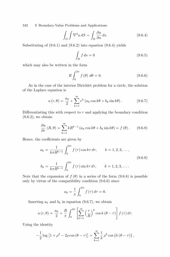
342 9 Boundary-Value Problems and Applications∫D
∫∇2u dS =
∫B
∂u
∂nds. (9.6.4)
Substituting of (9.6.1) and (9.6.2) into equation (9.6.4) yields∫B
f ds = 0 (9.6.5)
which may also be written in the form
R
∫ 2π
0f (θ) dθ = 0. (9.6.6)
As in the case of the interior Dirichlet problem for a circle, the solutionof the Laplace equation is
u (r, θ) =a0
2+
∞∑k=1
rk (ak cos kθ + bk sin kθ) . (9.6.7)
Differentiating this with respect to r and applying the boundary condition(9.6.2), we obtain
∂u
∂r(R, θ) =
∞∑k=1
kRk−1 (ak cos kθ + bk sin kθ) = f (θ) . (9.6.8)
Hence, the coefficients are given by
ak =1
kπRk−1
∫ 2π
0f (τ) cos kτ dτ, k = 1, 2, 3, . . . ,
(9.6.9)
bk =1
kπRk−1
∫ 2π
0f (τ) sin kτ dτ, k = 1, 2, 3, . . . .
Note that the expansion of f (θ) in a series of the form (9.6.8) is possibleonly by virtue of the compatibility condition (9.6.6) since
a0 =1π
∫ 2π
0f (τ) dτ = 0.
Inserting ak and bk in equation (9.6.7), we obtain
u (r, θ) =a0
2+
R
π
∫ 2π
0
[ ∞∑k=1
( r
R
)k
cos k (θ − τ)
]f (τ) dτ.
Using the identity
−12
log[1 + ρ2 − 2ρ cos (θ − τ)
]=
∞∑k=1
1k
ρk cos k (θ − τ) ,

9.7 Dirichlet Problem for a Rectangle 343
with ρ = (r/R), we find that
u (r, θ) =a0
2− R
2π
∫ 2π
0log
[R2 − 2rR cos (θ − τ) + r2] f (τ) dτ. (9.6.10)
in which a constant factor R2 in the argument of the logarithm was elimi-nated by virtue of equation (9.6.6).
In a similar manner, for the exterior Neumann problem, we can readilyfind the solution in the form
u (r, θ) =a0
2+
R
2π
∫ 2π
0log
[R2 − 2rR cos (θ − τ) + r2] f (τ) dτ. (9.6.11)
9.7 Dirichlet Problem for a Rectangle
We first consider the boundary-value problem
∇2u = uxx + uyy = 0, 0 < x < a, 0 < y < b, (9.7.1)u (x, 0) = f (x) , u (x, b) = 0, 0 ≤ x ≤ a, (9.7.2)u (0, y) = 0, u (a, y) = 0, 0 ≤ y ≤ b. (9.7.3)
We seek a nontrivial separable solution in the form
u (x, y) = X (x) Y (y)
Substituting u (x, y) in the Laplace equation, we obtain
X ′′ − λX = 0, (9.7.4)Y ′′ + λY = 0, (9.7.5)
where λ is a separation constant. Since the boundary conditions are homo-geneous for x = 0 and x = a, we choose λ = −α2 with α > 0 in order toobtain nontrivial solutions of the eigenvalue problem
X ′′ + α2X = 0,
X (0) = X (a) = 0.
It is easily found that the eigenvalues are
α =nπ
a, n = 1, 2, 3, . . . .
and the corresponding eigenfunctions are sin (nπx/a). Hence
Xn (x) = Bn sin(nπx
a
).

344 9 Boundary-Value Problems and Applications
The solution of equation (9.7.5) is Y (y) = C cosh αy+D sinhαy, whichmay also be written in the form
Y (y) = E sinhα (y + F ) ,
where E =(D2 − C2
) 12 and F = (1/α) tanh−1 (C/D). Applying the re-
maining homogeneous boundary condition
u (x, b) = X (x) Y (b) = 0,
we obtain
Y (b) = E sinhα (b + F ) = 0,
and hence,
F = −b, E = 0
for a nontrivial solution u (x, y). Thus, we have
Yn (y) = En sinhnπ
a(y − b)
.
Because of linearity, the solution becomes
u (x, y) =∞∑
n=1
an sin(nπx
a
)sinh
nπ
a(y − b)
,
where an = BnEn. Now, we apply the nonhomogeneous boundary conditionto obtain
u (x, 0) = f (x) =∞∑
n=1
an sinh(−nπb
a
)sin
(nπx
a
).
This is a Fourier sine series and hence,
an =−2
a sinh(
nπba
) ∫ a
0f (x) sin
(nπx
a
)dx.
Thus, the formal solution is given by
u (x, y) =∞∑
n=1
a∗n
sinh
nπa (b − y)
sinh
(nπba
) sin(nπx
a
), (9.7.6)
where
a∗n =
2a
∫ a
0f (x) sin
(nπx
a
)dx.

9.7 Dirichlet Problem for a Rectangle 345
To prove the existence of solution (9.7.6), we first note that
sinh nπa (b − y)
sinh nπba
= e−nπy/a
[1 − e−(2nπ/a)(b−y)
1 − e−2nπb/a
]≤ C1e
−nπy/a,
where C1 is a constant. Since f (x) is bounded, we have
|a∗n| ≤ 2
a
∫ a
0|f (x)| dx = C2.
Thus, the series for u (x, y) is dominated by the series
∞∑n=1
Me−nπy0/a for y ≥ y0 > 0, M = constant,
and hence, u (x, y) converges uniformly in x and y whenever 0 ≤ x ≤ a,y ≥ y0 > 0. Consequently, u (x, y) is continuous in this region and satisfiesthe boundary values u (0, y) = u (a, y) = u (x, b) = 0.
Now differentiating u twice with respect to x, we obtain
uxx (x, y) =∞∑
n=1
−a∗n
(nπ
a
)2 sinh nπa (b − y)
sinh nπba
sin(nπx
a
)and differentiating u twice with respect to y, we obtain
uyy (x, y) =∞∑
n=1
a∗n
(nπ
a
)2 sinh nπa (b − y)
sinh nπba
sin(nπx
a
).
It is evident that the series for uxx and uyy are both dominated by
∞∑n=1
M∗n2e−nπy0/a
and hence, converge uniformly for any 0 < y0 < b. It follows that uxxanduyy exist, and hence, u satisfies the Laplace equation.
It now remains to show that u (x, 0) = f (x). Let f (x) be a continuousfunction and let f ′ (x) be piecewise continuous on [0, a]. If, in addition,f (0) = f (a) = 0, then, the Fourier series for f (x) converges uniformly.Putting y = 0 in the series for u (x, y), we obtain
u (x, 0) =∞∑
n=1
a∗n sin
(nπx
a
).
Since u (x, 0) converges uniformly to f (x), we write, for ε > 0,
|sm (x, 0) − sn (x, 0)| < ε for m, n > Nε,

346 9 Boundary-Value Problems and Applications
where
sm (x, y) =∞∑
n=1
a∗n sin
(nπx
a
).
We also know that sm (x, y) − sn (x, y) satisfies the Laplace equation andthe boundary conditions at x = 0, x = a and y = b. Then, by the maximumprinciple,
|sm (x, y) − sn (x, y)| < ε for m, n > Nε
in the region 0 ≤ x ≤ a, 0 ≤ y ≤ b. Thus, the series for u (x, y) convergesuniformly, and as a consequence, u (x, y) is continuous in the region 0 ≤x ≤ a, 0 ≤ y ≤ b. Hence, we obtain
u (x, 0) =∞∑
n=1
a∗n sin
(nπx
a
)= f (x) .
Thus, the solution (9.7.6) is established.The general Dirichlet problem
∇2u = 0, 0 < x < a, 0 < y < b,
u (x, 0) = f1 (x) , u (x, a) = f2 (x) , 0 ≤ x ≤ a,
u (0, y) = f3 (y) , u (b, y) = f4 (y) , 0 ≤ y ≤ b
can be solved by separating it into four problems, each of which has onenonhomogeneous boundary condition and the rest zero. Thus, determiningeach solution as in the preceding problem and then adding the four solu-tions, the solution of the Dirichlet problem for a rectangle can be obtained.
9.8 Dirichlet Problem Involving the Poisson Equation
The solution of the Dirichlet problem involving the Poisson equation can beobtained for simple regions when the solution of the corresponding Dirichletproblem for the Laplace equation is known.
Consider the Poisson equation
∇2u = uxx + uuu = f (x, y) in D,
with the condition
u = g (x, y) on B.
Assume that the solution can be written in the form
u = v + w,
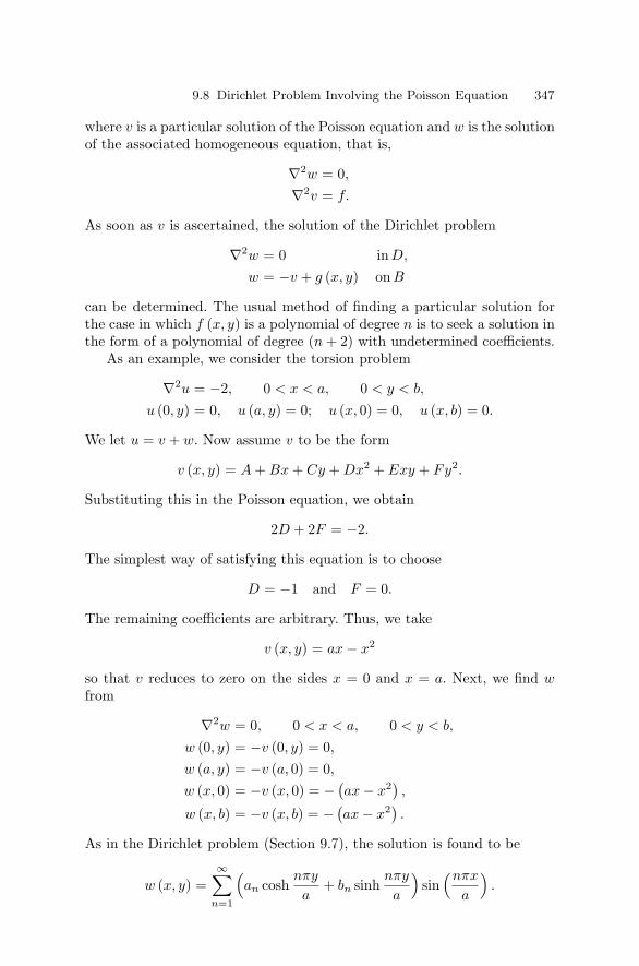
9.8 Dirichlet Problem Involving the Poisson Equation 347
where v is a particular solution of the Poisson equation and w is the solutionof the associated homogeneous equation, that is,
∇2w = 0,
∇2v = f.
As soon as v is ascertained, the solution of the Dirichlet problem
∇2w = 0 inD,
w = −v + g (x, y) on B
can be determined. The usual method of finding a particular solution forthe case in which f (x, y) is a polynomial of degree n is to seek a solution inthe form of a polynomial of degree (n + 2) with undetermined coefficients.
As an example, we consider the torsion problem
∇2u = −2, 0 < x < a, 0 < y < b,
u (0, y) = 0, u (a, y) = 0; u (x, 0) = 0, u (x, b) = 0.
We let u = v + w. Now assume v to be the form
v (x, y) = A + Bx + Cy + Dx2 + Exy + Fy2.
Substituting this in the Poisson equation, we obtain
2D + 2F = −2.
The simplest way of satisfying this equation is to choose
D = −1 and F = 0.
The remaining coefficients are arbitrary. Thus, we take
v (x, y) = ax − x2
so that v reduces to zero on the sides x = 0 and x = a. Next, we find wfrom
∇2w = 0, 0 < x < a, 0 < y < b,
w (0, y) = −v (0, y) = 0,w (a, y) = −v (a, 0) = 0,
w (x, 0) = −v (x, 0) = − (ax − x2) ,
w (x, b) = −v (x, b) = − (ax − x2) .
As in the Dirichlet problem (Section 9.7), the solution is found to be
w (x, y) =∞∑
n=1
(an cosh
nπy
a+ bn sinh
nπy
a
)sin
(nπx
a
).

348 9 Boundary-Value Problems and Applications
Application of the nonhomogeneous boundary conditions yields
w (x, 0) = − (ax − x2) =
∞∑n=1
an sin(nπx
a
),
w (x, b) = − (ax − x2) =
∞∑n=1
(an cosh
nπb
a+ bn sinh
nπb
a
)sin
(nπx
a
),
from which we find
an =2a
∫ a
0
(x2 − ax
)sin
(nπx
a
)dx
=
0, ifn is even−8a2
π3n3 ifn is odd
and (an cosh
nπb
a+ bn sinh
nπb
a
)=
2a
∫ a
0
(x2 − ax
)sin
(nπx
a
)dx.
Thus, we have
bn =
(1 − cosh nπb
a
)an
sinh(
nπba
) .
Hence, the solution of the Dirichlet problem for the Poisson equation isgiven by
u (x, y) = (a − x) x
− 8a2
π3
∞∑n=1
[sinh (2n − 1) π(b−y)
a + sinh (2n − 1) πya
]sinh (2n − 1) πb
a
sin (2n − 1) πxa
(2n − 1)3.
9.9 The Neumann Problem for a Rectangle
Consider the Neumann problem
∇2u = 0, 0 < x < a, 0 < y < b, (9.9.1)ux (0, y) = f1 (y) , ux (a, y) = f2 (y) , 0 ≤ y ≤ b, (9.9.2)uy (x, 0) = g1 (x) , uy (x, b) = g2 (x) , 0 ≤ x ≤ a. (9.9.3)
The compatibility condition that must be fulfilled in this case is∫ a
0[g1 (x) − g2 (x)] dx +
∫ b
0[f1 (y) − f2 (y)] dy = 0. (9.9.4)
We assume a solution in the form

9.9 The Neumann Problem for a Rectangle 349
u (x, y) = u1 (x, y) + u2 (x, y) , (9.9.5)
where u1 (x, y) is a solution of
∇2u1 = 0,
∂u1
∂x(0, y) = 0,
∂u1
∂x(a, y) = 0, (9.9.6)
∂u1
∂x(x, 0) = g1 (x) ,
∂u1
∂x(x, b) = g2 (x) ,
and where g1 and g2 satisfy the compatibility condition∫ a
0[g1 (x) − g2 (x)] dx = 0. (9.9.7)
The function u2 (x, y) is a solution of
∇2u2 = 0,
∂u2
∂x(0, y) = f1 (y)
∂u2
∂x(a, y) = f2 (y) (9.9.8)
∂u2
∂y(x, 0) = 0,
∂u2
∂y(x, b) = 0,
where f1 and f2 satisfy the compatibility condition∫ b
0[f1 (y) − f2 (y)] dy = 0. (9.9.9)
Hence, u1 (x, y) and u2 (x, y) can be determined. Conditions (9.9.7) and(9.9.9) ensure that condition (9.9.4) is fulfilled. Thus, the problem is solved.
However, the solution obtained in this manner is rather restrictive. Ingeneral, condition (9.9.4) does not imply conditions (9.9.7) and (9.9.9).Thus, generally speaking, it is not possible to obtain a solution of theNeumann problem for a rectangle by the method described above.
To obtain a general solution, Grunberg (1946) proposed the followingmethod. Suppose we assume a solution in the form
u (x, y) =Y0
2(y) +
∞∑n=1
Xn (x) Yn (y) , (9.9.10)

350 9 Boundary-Value Problems and Applications
where Xn (x) = cos (nπx/a) is an eigenfunction of the eigenvalue problem
X ′′ + λX = 0,
X ′ (0) = X ′ (a) = 0,
corresponding to the eigenvalue λn = (nπ/a)2. Then, from equation(9.9.10), we see that
Yn (y) =2a
∫ a
0u (x, y) Xn (x) dx,
=2a
∫ a
0u (x, y) cos
(nπx
a
)dx. (9.9.11)
Multiplying both sides of equation (9.9.1) by 2 cos (nπx/a) and integratingwith respect to x from 0 to a, we obtain
2a
∫ a
0(uxx + uyy) cos
(nπx
a
)dx = 0,
or,
Y ′′n +
2a
∫ a
0uxx cos
(nπx
a
)dx = 0.
Integrating the second term by parts and applying the boundary conditions(9.9.2), we obtain
Y ′′n (y) −
(nπ
a
)2Yn (y) = Fn (y) , (9.9.12)
where Fn (y) = 2 [f1 (y) − (−1)nf2 (y)] /a. This is an ordinary differential
equation whose solution may be written in the form
Yn (y) = An cosh(nπy
a
)+ Bn sinh
(nπy
a
)+
2πn
∫ y
0Fn (τ) sinh
nπ
a(y − τ)
dτ. (9.9.13)
The coefficients Anand Bn are determined from the boundary conditions
Y ′n (0) =
2a
∫ a
0uy (x, 0) cos
(nπx
a
)dx
=2a
∫ a
0g1 (x) cos
(nπx
a
)dx (9.9.14)
and
Y ′n (b) =
2a
∫ a
0g2 (x) cos
(nπx
a
)dx. (9.9.15)

9.10 Exercises 351
For n = 0, equation (9.9.12) takes the form
Y ′′0 (y) =
2a
[f1 (y) − f2 (y)]
and hence,
Y ′0 (y) =
2a
∫ y
0[f1 (τ) − f2 (τ)] dτ + C,
where C is an integration constant. Employing the condition (9.9.14) forn = 0, we find
C =2a
∫ a
0g1 (x) dx.
Thus, we have
Y ′0 (y) =
2a
∫ y
0[f1 (τ) − f2 (τ)] dτ +
∫ a
0g1 (x) dx
.
Consequently,
Y ′0 (b) =
2a
∫ b
0[f1 (τ) − f2 (τ)] dτ +
∫ a
0g1 (x) dx
.
Also from equation (9.9.14), we have
Y ′0 (b) =
2a
∫ a
0g2 (x) dx.
It follows from these two expressions for Y ′0 (b) that∫ b
0[f1 (y) − f2 (y)] dy +
∫ a
0[g1 (x) − g2 (x)] dx = 0.
which is the necessary condition for the existence of a solution to the Neu-mann problem for a rectangle.
9.10 Exercises
1. Reduce the Neumann problem to the Dirichlet problem in the two-dimensional case.
2. Reduce the wave equation
un = c2 (uxx + uyy + uzz)

352 9 Boundary-Value Problems and Applications
to the Laplace equation
uxx + uyy + uzz + uττ = 0
by letting τ = ict where i =√−1. Obtain the solution of the wave equa-
tion in cylindrical coordinates via the solution of the Laplace equation.Assume that u (r, θ, z, τ) is independent of z.
3. Prove that, if u (x, t) satisfies
ut = k uxx
for 0 ≤ x ≤ 1, 0 ≤ t ≤ t0, then the maximum value of u is attainedeither at t = 0 or at the end points x = 0 or x = 1 for 0 ≤ t ≤ t0. Thisis called the maximum principle for the heat equation.
4. Prove that a function which is harmonic everywhere on a plane and isbounded either above or below is a constant. This is called the Liouvilletheorem.
5. Show that the compatibility condition for the Neumann problem
∇2u = f inD
∂u
∂n= g onB
is ∫D
f dS +∫
B
g ds = 0,
where B is the boundary of domain D.
6. Show that the second degree polynomial
P = Ax2 + Bxy + Cy2 + Dyz + Fz2 + Fxz
is harmonic if
E = − (A + C)
and obtain
P = A(x2 − z2) + Bxy + C
(y2 − z2) + Dyz + Fxz.
7. Prove that a solution of the Neumann problem
∇2u = f inD
u = g onB
differs from another solution by at most a constant.

9.10 Exercises 353
8. Determine the solution of each of the following problems:
(a) ∇2u = 0, 1 < r < 2, 0 < θ < π,
u (1, θ) = sin θ, u (2, θ) = 0, 0 ≤ θ ≤ π,
u (r, 0) = 0, u (r, π) = 0, 1 ≤ r ≤ 2.
(b) ∇2u = 0, 1 < r < 2, 0 < θ < π,
u (1, θ) = 0, u (2, θ) = θ (θ − π) , 0 ≤ θ ≤ π,
u (r, 0) = 0, u (r, π) = 0, 1 ≤ r ≤ 2.
(c) ∇2u = 0, 1 < r < 3, 0 < θ < π/2,
u (1, θ) = 0, u (3, θ) = 0, 0 ≤ θ ≤ π/2,
u (r, 0) = (r − 1) (r − 3) , u(r, π
2
)= 0, 1 ≤ r ≤ 3.
(d) ∇2u = 0, 1 < r < 3, 0 < θ < π/2,
u (1, θ) = 0, u (3, θ) = 0, 0 ≤ θ ≤ π,
u (r, 0) = 0, u(r, π
2
)= f (r) , 1 ≤ r ≤ 3.
9. Solve the boundary-value problem
∇2u = 0, a < r < b, 0 < θ < α,
u (a, θ) = f (θ) , u (b, θ) = 0, 0 ≤ θ ≤ α,
u (r, α) = 0, u (r, 0) = f (r) , a ≤ r ≤ b.
10. Verify directly that the Poisson integral is a solution of the Laplaceequation.
11. Solve∇2u = 0, 0 < r < a, 0 < θ < π,
u (r, 0) = 0, u (r, π) = 0,
u (a, θ) = θ (π − θ) , 0 ≤ θ ≤ π,
u (0, θ) is bounded.

354 9 Boundary-Value Problems and Applications
12. Solve
∇2u + u = 0, 0 < r < a, 0 < θ < α,
u (r, 0) = 0, u (r, α) = 0,
u (a, θ) = f (θ) , 0 ≤ θ ≤ α,
u (0, θ) is bounded.
13. Find the solution of the Dirichlet problem
∇2u = −2, r < a, 0 < θ < 2π,
u (a, 0) = 0.
14. Solve the following problems:
(a) ∇2u = 0, 1 < r < 2, 0 < θ < 2π,
ur (1, θ) = sin θ, ur (2, θ) = 0, 0 ≤ θ ≤ 2π,
(b) ∇2u = 0, 1 < r < 2, 0 < θ < 2π,
ur (1, θ) = 0, ur (2, θ) = θ − π, 0 ≤ θ ≤ 2π.
15. Solve
∇2u = 0, a < r < b, 0 < θ < 2π,
ur (a, θ) = f (θ) , ur (b, θ) = g (θ) , 0 ≤ θ ≤ 2π,
where ∫r=a
f ds +∫
r=b
g ds = 0.
16. Solve the Robin problem for a semicircular disk
∇2u = 0, r < R, 0 < θ < π,
ur (R, θ) = sin θ, 0 ≤ θ ≤ π,
u (r, 0) = 0, u (r, π) = 0.

9.10 Exercises 355
17. Solve
∇2u = 0, a < r < b, 0 < θ < α,
ur (a, θ) = 0, ur (b, θ) = f (θ) , 0 ≤ θ ≤ α,
u (r, 0) = 0, u (r, α) = 0, a < r < b.
18. Determine the solution of the mixed boundary-value problem
∇2u = 0, r < R, 0 < θ < 2π,
ur (R, θ) + hu (R, θ) = f (θ) , h = constant.
19. Solve
∇2u = 0, a < r < b, 0 < θ < 2π,
ur (a, θ) + hu (a, θ) = f (θ) , ur (b, θ) + hu (b, θ) = g (θ) .
20. Find a solution of the Neumann problem
∇2u = −r2 sin 2θ, r1 < r < r2, 0 < θ < 2π,
ur (r1, θ) = 0, ur (r2, θ) = 0, 0 ≤ θ ≤ 2π.
21. Solve the Robin problem
∇2u = − r2 sin 2θ,
u (r1, θ) = 0, ur (r2, θ) = 0.
22. Solve the following Dirichlet problems:(a) ∇2u = 0, 0 < x < 1, 0 < y < 1,
u (x, 0) = x (x − 1) , u (x, 1) = 0, 0 ≤ x ≤ 1,
u (0, y) = 0, u (1, y) = 0, 0 ≤ y ≤ 1.
(b) ∇2u = 0, 0 < x < 1, 0 < y < 1,
u (x, 0) = 0, u (x, 1) = sin (πx) , 0 ≤ x ≤ 1,
u (0, y) = 0, u (1, y) = 0, 0 ≤ y ≤ 1.

356 9 Boundary-Value Problems and Applications
(c) ∇2u = 0, 0 < x < 1, 0 < y < 1,
u (x, 0) = 0, u (x, 1) = 0, 0 ≤ x ≤ 1,
u (0, y) =(cos πy
2 − 1)
cos(
πy2
), u (1, y) = 0, 0 ≤ y ≤ 1.
(d) ∇2u = 0, 0 < x < 1, 0 < y < 1,
u (x, 0) = 0, u (x, 1) = 0, 0 ≤ x ≤ 1,
u (0, y) = 0, u (1, y) = sinπy cos πy, 0 ≤ y ≤ 1.
23. Solve the following Neumann problems:
(a) ∇2u = 0, 0 < x < π, 0 < y < π,
ux (0, y) =(y − π
2
), ux (π, y) = 0, 0 ≤ y ≤ π,
uy (x, 0) = x, uy (x, π) = x, 0 ≤ x ≤ π.
(b) ∇2u = 0, 0 < x < π, 0 < y < π,
ux (0, y) = 0, ux (π, y) = 2 cos y, 0 ≤ y ≤ π,
uy (x, 0) = 0, uy (x, π) = 0, 0 ≤ x ≤ π.
(c) ∇2u = 0, 0 < x < π, 0 < y < π,
ux (0, y) = 0, ux (π, y) = 0, 0 ≤ y ≤ π,
uy (x, 0) = cos x, uy (x, π) = 0, 0 ≤ x ≤ π.
(d) ∇2u = 0, 0 < x < π, 0 < y < π,
ux (0, y) = y, ux (π, y) = y, 0 ≤ y ≤ π,
uy (x, 0) = x, uy (x, π) = x. 0 ≤ x ≤ π.
24. The steady-state temperature distribution in a rectangular plate oflength a and width b is described by
∇2u = 0, 0 < x < a, 0 < y < b.
At x = 0, the temperature is kept at zero degrees, while at x = a, theplate is insulated. The temperature is prescribed at y = 0. At y = b,

9.10 Exercises 357
heat is allowed to radiate freely into the surrounding medium of zerodegree temperature. That is, the boundary conditions are
u (0, y) = 0, ux (a, y) = 0, 0 ≤ y ≤ b,
u (x, 0) = f (x) , uy (x, b) + hu (x, b) = 0, 0 ≤ x ≤ a.
Determine the temperature distribution.
25. Solve the Dirichlet problem
∇2u = −2y, 0 < x < 1, 0 < y < 1,
u (0, y) = 0, u (1, y) = 0, 0 ≤ y ≤ 1,
u (x, 0) = 0, u (x, 1) = 0, 0 ≤ x ≤ 1.
26. Find the harmonic function which vanishes on the hypotenuse and hasprescribed values on the other two sides of an isosceles right-angledtriangle formed by x = 0, y = 0, and y = a − x, where a is a constant.
27. Find a solution of the Neumann problem
∇2u =(x2 − y2) , 0 < x < a, 0 < y < a,
ux (0, y) = 0, ux (a, y) = 0, 0 ≤ y ≤ a,
uy (x, 0) = 0, uy (x, a) = 0, 0 ≤ x ≤ a.
28. Solve the third boundary-value problem
∇2u = 0, 0 < x < 1, 0 < y < 1,
ux (0, y) + h u (0, y) = 0, 0 ≤ y ≤ 1, h = constant
ux (1, y) + h u (1, y) = 0, 0 ≤ y ≤ 1,
uy (x, 0) + h u (x, 0) = 0, 0 ≤ x ≤ 1,
uy (x, 1) + h u (x, 1) = f (x) , 0 ≤ x ≤ 1.

358 9 Boundary-Value Problems and Applications
29. Determine the solution of the boundary-value problem
∇2u = 1, 0 < x < π, 0 < y < π,
u (0, y) = 0, ux (π, y) = 0, 0 ≤ y ≤ π,
uy (x, 0) = 0, uy (x, π) + h u (x, π) = f (x) , 0 ≤ x ≤ π.
30. Obtain the integral representation of the Neumann problem
∇2u = f in D,
∂u
∂n= g on boundary B of D.
31. Find the solution in terms of the Green’s function of the Poisson prob-lem
∇2u = f in D,
∂u
∂n+ hu = g on boundary B of D.
32. Find the steady-state temperature distribution inside a circular annularregion governed by the boundary-value problem
urr +1r
ur +1r2 uθθ = 0, 1 < r < 2, −π < 0 < π,
u (1, θ) = sin2 θ, ur (2, θ) = 0, −π < θ < π.
33. Consider a radially symmetric steady-state problem in a solid homoge-neous cylinder of radius unity and height h. The temperature distribu-tion function u (r, z) satisfies the equation
∇2u = urr +1r
ur + uzz = 0, 0 < r < 1, 0 < z < h.
Solve the Dirichlet boundary-value problem with the following bound-ary conditions:
(a) u (1, z) = f (z) , u (r, 0) = 0, u (r, h) = 0,
(b) u (1, z) = 0, u (r, 0) = g (r) , u (r, h) = 0,
(c) u (1, z) = 0, u (r, 0) = 0, u (r, h) = w (r) ,
(d) u (1, z) = a sin( 3πz
h
), u (r, 0) = 0 = u (r, h) .

9.10 Exercises 359
34. Show that the solution of the problem 33(c) is given by
u (r, z) =∞∑
n=1
anJ0 (knr)sinh knz
sinh knh,
where J0 (kn) = 0, n = 1, 2, 3, . . ..
35. Solve the following boundary-value problem:
(a) ∇2u = 0, 0 < r < 1, 0 < z < 1,
u (1, z) = 0 = u (r, 0) , u (r, 1) = 1 − r2, 0 ≤ r ≤ 1.
(b) ∇2u = 0, 0 < r < 1, 0 < z < π,
u (1, z) = A = constant, u (r, 0) = 0, uz (r, π) = 0.
(c) ∇2u = 0, 0 < r < a, 0 < z < h,
u (a, z) = f (z) , u (r, 0) = 0 = u (r, h) , 0 ≤ r ≤ a.
(d) ∇2u = 0, 0 < r < a, 0 < z < h,
u (a, z) = z (h − z) , u (r, 0) = 0 = u (r, h) .
In each of the above problems (a)–(d),
∇2u = urr +1r
ur + uzz.

10
Higher-Dimensional Boundary-ValueProblems
“As long as a branch of knowledge offers an abundance of problems, it isfull of vitality.”
David Hilbert
10.1 Introduction
The treatment of problems in more than two space variables is much moreinvolved than problems in two space variables. Here a number of multi-dimensional problems involving the Laplace equation, wave and heat equa-tions with various boundary conditions will be presented. Included are theDirichlet problem for a cube, for a cylinder and for a sphere, wave and heatequations in three dimensional rectangular, cylindrical polar and sphericalpolar coordinates. The solution of the three-dimensional Schrodinger equa-tion in a central field with applications to hydrogen and helium atoms isdiscussed. We also consider the forced vibration of a rectangular membranedescribed by the three-dimensional, nonhomogeneous wave equation withmoving boundaries.
10.2 Dirichlet Problem for a Cube
The steady-state temperature distribution in a cube is described by theLaplace equation
∇2u = uxx + uyy + uzz = 0 (10.2.1)
for 0 < x < π, 0 < y < π, 0 < z < π. The faces are kept at zero degreetemperature except for the face z = 0, that is,

362 10 Higher-Dimensional Boundary-Value Problems
u (0, y, z) = u (π, y, z) = 0u (x, 0, z) = u (x, π, z) = 0u (x, y, π) = 0, u (x, y, 0) = f (x, y) , 0 ≤ x ≤ π, 0 ≤ y ≤ π.
We assume a nontrivial separable solution in the form
u (x, y, z) = X (x) Y (y) Z (z) .
Substituting this in the Laplace equation, we obtain
X ′′Y Z + XY ′′Z + XY Z ′′ = 0.
Division by XY Z yields
X ′′
X+
Y ′′
Y= −Z ′′
Z.
Since the right side depends only on z and the left side is independent ofz, both terms must be equal to a constant. Thus, we have
X ′′
X+
Y ′′
Y= −Z ′′
Z= λ.
By the same reasoning, we have
X ′′
X= λ − Y ′′
Y= µ.
Hence, we obtain the three ordinary differential equations
X ′′ − µX = 0,
Y ′′ − (λ − µ) Y = 0,
Z ′′ + λZ = 0.
Using the boundary conditions, the eigenvalue problem for X,
X ′′ − µX = 0,
X (0) = X (π) = 0,
yields the eigenvalues µ = −m2 for m = 1, 2, 3, . . . and the correspondingeigenfunctions sinmx.
Similarly, the eigenvalue problem for Y
Y ′′ − (λ − µ) Y = 0,
Y (0) = Y (π) = 0,
gives the eigenvalues λ−µ = −n2 where n = 1, 2, 3, . . . and the correspond-ing eigenfunctions sinny.

10.3 Dirichlet Problem for a Cylinder 363
Since λ is given by − (m2 + n2
), it follows that the solution of Z ′′+λZ =
0 satisfying the condition Z (π) = 0 is
Z (z) = C sinh[√
m2 + n2 (π − z)].
Thus, the solution of the Laplace equation satisfying the homogeneousboundary conditions takes the form
u (x, y, z) =∞∑
m=1
∞∑n=1
amn sinh(√
m2 + n2 (π − z))
sin mx sin ny.
Applying the nonhomogeneous boundary condition, we formally obtain
f (x, y) =∞∑
m=1
∞∑n=1
amn sinh(√
m2 + n2 π)
sin mx sin ny.
The coefficient of the double Fourier series is thus given by
amn sinh(√
m2 + n2 π)
=4π2
∫ π
0
∫ π
0f (x, y) sinmx sin ny dx dy.
Therefore, the formal solution to the Dirichlet problem for a cube may bewritten in the form
u (x, y, z) =∞∑
m=1
∞∑n=1
bmn
sinh(√
m2 + n2 (π − z))
sinh(√
m2 + n2 π) sin mx sin ny, (10.2.2)
where
bmn = amn sinh(√
m2 + n2 π)
.
10.3 Dirichlet Problem for a Cylinder
Example 10.3.1. We consider the problem of determining the electric po-tential u inside a charge-free cylinder. The potential u satisfies the Laplaceequation in cylindrical polar coordinates
∇2u = urr +1r
ur +1r2 uθθ + uzz = 0, (10.3.1)
for 0 ≤ r < a, 0 < z < l. Let the lateral surface r = a and the top z = lbe grounded, that is, zero potential. Let the potential on the base z = 0 begiven by
u (r, θ, 0) = f (r, θ) , (10.3.2)
where f (a, θ) = 0.

364 10 Higher-Dimensional Boundary-Value Problems
We assume a nontrivial separable solution in the form
u (r, θ, z) = R (r) Θ (θ) Z (z) .
Substituting this in the Laplace equation yields
R′′ + 1r R′
R+
1r2
Θ′′
Θ= −Z ′′
Z= λ.
It follows that
r2R′′ + rR′
R− r2λ = −Θ′′
Θ= µ.
Thus, we obtain the equations
r2R′′ + rR′ − (λ r2 + µ
)R = 0, (10.3.3)
Θ′′ + µΘ = 0, (10.3.4)Z ′′ + λZ = 0. (10.3.5)
Using the periodicity conditions, the eigenvalue problem for Θ (θ),
Θ′′ + µΘ = 0,
Θ (0) = Θ (2π) , Θ′ (0) = Θ′ (2π) ,
yields the eigenvalues µ = n2 for n = 0, 1, 2, . . . with the correspondingeigenfunctions sinnθ, cos nθ. Thus,
Θ (θ) = A cos nθ + B sin nθ. (10.3.6)
Suppose λ is real and negative and let λ = −β2 where β > 0. If the conditionZ (l) = 0 is imposed, then the solution of equation (10.3.5) can be writtenin the form
Z (z) = C sinhβ (l − z) . (10.3.7)
Next we introduce the new independent variable ξ = βr. Equation(10.3.3) transforms into
ξ2 d2R
dξ2 + ξdR
dξ+
(ξ2 − n2)R = 0
which is the Bessel equation of order n. The general solution is
Rn (ξ) = DJn (ξ) + E Yn (ξ)
where Jn and Yn are the Bessel functions of the first and second kindrespectively. In terms of the original variable, we have

10.3 Dirichlet Problem for a Cylinder 365
Rn (r) = DJn (βr) + E Yn (βr) .
Since Yn (βr) is unbounded at r = 0, we choose E = 0. The conditionR (a) = 0 requires that
Jn (βa) = 0.
For each n ≥ 0, there exist positive zeros. Arranging these in an infiniteincreasing sequence, we have
0 < αn1 < αn2 < . . . < αnm < . . . .
Thus, we obtain
βnm = (αnm/a) .
Consequently,
Rn (r) = DJn (αnmr/a) .
The solution u then finally takes the form
u (r, θ, z) =∞∑
n=0
∞∑m=1
Jn
( r
aαnm
)(anm cos nθ + bnm sin nθ)
× sinh[(l − z)
aαnm
].
To satisfy the nonhomogeneous boundary condition, it is required that
f (r, θ) =∞∑
n=0
∞∑m=1
Jn
( r
aαnm
)(anm cos nθ + bnm sin nθ) sinh
(l
aαnm
).
The coefficients anm and bnm are given by
a0m =1
πa2 sinh( 1
a α0m
)[J1 (α0m)]2
∫ a
0
∫ 2π
0f (r, θ) J0
( r
aα0m
)r dr dθ,
anm =2
πa2 sinh( 1
a αnm
)[Jn+1 (αnm)]2
∫ a
0
∫ 2π
0f (r, θ) Jn
( r
aαnm
)× cos nθ r dr dθ,
bnm =2
πa2 sinh( 1
a αnm
)[Jn+1 (αnm)]2
∫ a
0
∫ 2π
0f (r, θ) Jn
( r
aαnm
)× sin nθ r dr dθ.
Example 10.3.2. We shall illustrate the same problem with different bound-ary conditions. Consider the problem

366 10 Higher-Dimensional Boundary-Value Problems
∇2u = 0, 0 ≤ r < a, 0 < z < π,
u (r, θ, 0) = 0, u (r, θ, π) = 0,u (a, θ, z) = f (θ, z) .
As before, by the separation of variables, we obtain
r2R′′ + rR′ − (λr2 + µ
)R = 0,
Θ′′ + µΘ = 0,
Z ′′ + λZ = 0.
By the periodicity conditions, again as in the previous example, the Θ equa-tion yields the eigenvalues µ = n2 with n = 0, 1, 2, . . .; the correspondingeigenfunctions are sinnθ, cos nθ. Thus, we have
Θ (θ) = An cos n cos θ + Bn sin nθ.
Now let λ = β2 with β > 0. Then, the boundary value problem
Z ′′ + β2Z = 0Z (0) = 0, Z (π) = 0,
has the solution
Z (z) = Cm sin mz, m = 1, 2, 3, . . . .
Finally, we have
r2R′′ + rR′ − (m2r2 + n2)R = 0,
or
R′′ +1rR′ −
(m2 +
n2
r2
)R = 0,
the general solution of which is
R (r) = DIn (mr) + EKn (mr) ,
where In and Kn are the modified Bessel functions of the first and secondkind, respectively.
Since R must remain finite at r = 0, we set E = 0. Then R takes theform
R (r) = DIn (mr) .
Applying the nonhomogeneous condition, we find the solution

10.4 Dirichlet Problem for a Sphere 367
u (r, θ, z) =∞∑
m=1
(am0
2
) I0 (mr)I0 (ma)
sin mz
+∞∑
m=1
∞∑n=1
(amn cos nθ + bmn sin nθ)In (mr)In (ma)
sin mz,
where
amn =2π2
∫ π
0
∫ 2π
0f (θ, z) sinmz cos nθ dθ dz,
bmn =2π2
∫ π
0
∫ 2π
0f (θ, z) sinmz sin nθ dθ dz.
10.4 Dirichlet Problem for a Sphere
Example 10.4.3. To determine the potential in a sphere, we transform theLaplace equation into spherical coordinates. It has the form
∇2u = urr +2r
ur +1r2 uθθ +
cot θ
r2 uθ +1
r2 sin2 θuϕϕ, (10.4.1)
where 0 ≤ r < a, 0 < θ < π, and 0 < ϕ < 2π.Let the prescribed potential on the sphere be
u (a, θ, ϕ) = f (θ, ϕ) . (10.4.2)
We assume a nontrivial separable solution in the form
u (r, θ, ϕ) = R (r) Θ (θ) Φ (ϕ) .
Substitution of u in the Laplace equation yields
r2R′′ + 2rR′ − λR = 0, (10.4.3)sin2 θ Θ′′ + sin θ cos θ Θ′ +
(λ sin2 θ − µ
)Θ = 0, (10.4.4)
Φ′′ + µΦ = 0. (10.4.5)
The general solution of equation (10.4.5) is
Φ (ϕ) = A cos√
µ ϕ + Bn sin√
µ ϕ. (10.4.6)
The periodicity condition requires that√
µ = m, m = 0, 1, 2, . . . .
Since equation (10.4.3) is of Euler type, the solution is of the form
R (r) = rβ .

368 10 Higher-Dimensional Boundary-Value Problems
Inserting this is equation (10.4.3), we obtain
β2 + β − λ = 0.
The roots are β =(−1 +
√1 + 4λ
)/2 and − (1 + β). Hence, the general
solution of equation (10.4.3) is
R (r) = C rβ + D r−(1+β). (10.4.7)
The variable ξ = cos θ transforms equation (10.4.4) into the form(1 − ξ2)Θ′′ − 2ξΘ′ +
[β (β + 1) − m2
1 − ξ2
]Θ = 0 (10.4.8)
which is Legendre’s associated equation. The general solution with β = nfor n = 0, 1, 2, . . . is
Θ (θ) = E Pmn (cos θ) + F Qm
n (cos θ) .
Continuity of Θ (θ) at θ = 0, π corresponds to continuity of Θ (ξ) atξ = + 1. Since Qm
n (ξ) has a logarithmic singularity at ξ = 1, we chooseF = 0. Thus, the solution of equation (10.4.8) becomes
Θ (θ) = E Pmn (cos θ) .
Consequently, the solution of the Laplace equation in spherical coordinatesis
u (r, θ, ϕ) =∞∑
n=0
n∑m=0
rnPmn (cos θ) (anm cos mϕ + bnm sin mϕ) .
In order for u to satisfy the prescribed function on the boundary, it isnecessary that
f (θ, ϕ) =∞∑
n=0
n∑m=0
anPmn (cos θ) (anm cos mϕ + bnm sin mϕ)
for 0 ≤ θ ≤ π, 0 ≤ ϕ ≤ 2π. By the orthogonal properties of the functionsPm
n (cos θ) cos mϕ and Pmn (cos θ) sinmϕ, the coefficients are given by
anm =(2n + 1)
2πan
(n − m)!(n + m)!
∫ 2π
0
∫ π
0f (θ, ϕ) Pm
n (cos θ) cos mϕ sin θ dθ dϕ,
bnm =(2n + 1)
2πan
(n − m)!(n + m)!
∫ 2π
0
∫ π
0f (θ, ϕ) Pm
n (cos θ) sinmϕ sin θ dθ dϕ,
for m = 1, 2, . . ., and n = 1, 2, . . ., and
an0 =(2n + 1)
4πan
∫ 2π
0
∫ π
0f (θ, ϕ) Pn (cos θ) sin θ dθ dϕ,
for n = 0, 1, 2, . . ..

10.4 Dirichlet Problem for a Sphere 369
Example 10.4.4. Determine the potential of a grounded conducting spherein a uniform field that satisfies the problem
∇2u = 0, 0 ≤ r < a, 0 < θ < π, 0 < φ < 2π,
u (a, θ) = 0, u → −E0 r cos θ, as r → ∞.
Let the field be in the z direction so that the potential u will be inde-pendent of φ. Then, the Laplace equation takes the form
urr +2r
ur +1r2 uθθ +
cot θ
r2 uθ = 0.
We assume a nontrivial separable solution in the form
u (r, θ) = R (r) Θ (θ) .
Substitution of this in the Laplace equation yields
r2R′′ + 2rR′ − λR = 0,
sin2 θ Θ′′ + sin θ cos θ Θ′ + λ sin2 θ Θ = 0.
If we set λ = n (n + 1) with n = 0, 1, 2, . . ., then the second equation is theLegendre equation. The general solution of this equation is
Θ (θ) = An Pn (cos θ) + Bn Qn (cos θ) ,
where Pn and Qn are the Legendre functions of the first and second kindrespectively. In order for the solution not to be singular at θ = 0 and θ = π,we set Bn = 0. Thus, Θ (θ) becomes
Θ (θ) = An Pn (cos θ) .
The solution of the R-equation is obtained in the form
R (r) = Cn rn + Dn r−(n+1).
Thus, the potential function is
u (r, θ) =∞∑
n=0
(an rn + bn r−(n+1)
)Pn (cos θ) .
To satisfy the condition at infinity, we must have
a1 = −E0, and an = 0, for n ≥ 2
and hence,
u (r, θ) = −E0 r cos θ +∞∑
n=1
bn
rn+1 Pn (cos θ) .

370 10 Higher-Dimensional Boundary-Value Problems
The condition u (a, θ) = 0 yields
0 = −E0 a cos θ +∞∑
n=1
bn
an+1 Pn (cos θ) .
Using the orthogonality of the Legendre functions, we find that bn are givenby
bn =(2n + 1)
2E0 an+2
∫ π
−π
cos θ Pn (cos θ) d (cos θ) = E0 a3δn1,
since the integral vanishes for all n except n = 1. Hence, the potentialfunction is given by
u (r, θ) = −E0 r cos θ + E0a3
r2 cos θ.
Example 10.4.5. A dielectric sphere of radius a is placed in a uniform elec-tric field E0. Determine the potentials inside and outside the sphere.
The problem is to find potentials u1 and u2 that satisfy
∇2u1 = ∇2u2 = 0,
K∂u1
∂r=
∂u2
∂r, u1 = u2, on r = a,
u2 → −E0r cos θ as r → ∞,
where u1 and u2 are the potentials inside and outside the sphere, respec-tively, and K is the dielectric constant.
As in the preceeding example, the potential function is
u (r, θ) =∞∑
n=0
(an rn + bn r−(n+1)
)Pn (cos θ) . (10.4.9)
Since u1 must be finite at the origin, we take
u1 (r, θ) =∞∑
n=0
anrnPn (cos θ) for r ≤ a. (10.4.10)
For u2, which must approach infinity in the prescribed manner, we choose
u2 (r, θ) = −E0 r cos θ +∞∑
n=0
bn r−(n+1)Pn (cos θ) . (10.4.11)
From the two continuity conditions at r = a, we obtain
a1 = −E0 +b1
a3 , Ka1 = −E0 − 2b1
a3 ,
an = bn = 0, n ≥ 2.

10.4 Dirichlet Problem for a Sphere 371
The coefficients a1 and b1 are then found to be
a1 = − 3E0
K + 2, b1 = E0 a3 (K − 1)
(K + 2).
Hence, the potential for r ≤ a is given by
u1 (r, θ) = − 3E0
K + 2r cos θ,
and the potential for r ≥ a is given by
u2 (r, θ) = −E0 r cos θ + E0 a3 (K − 1)(K + 2)
r−2 cos θ.
Example 10.4.6. Determine the potential between concentric spheres heldat different constant potentials.
Here we need to solve
∇2u = 0, a < r < b,
u = A on r = a,
u = B on r = b.
In this case, the potential depends only on the radial distance. Hence, wehave
1r2
∂
∂r
(r2 ∂u
∂r
)= 0.
By elementary integration, we obtain
u (r) = c1 +c2
r,
where c1 and c2 are arbitrary constants.Applying the boundary conditions, we obtain
c1 =Bb − Aa
b − a, c2 = (A − B)
ab
b − a.
Thus, the solution is
u (r) =Bb − Aa
(b − a)+
(A − B) ab
(b − a) r
=(
Bb
r
)(r − a
b − a
)+
(Aa
r
)(b − r
b − a
).

372 10 Higher-Dimensional Boundary-Value Problems
10.5 Three-Dimensional Wave and Heat Equations
The wave equation in three space variables may be written as
utt = c2∇2u, (10.5.1)
where ∇2 is the three-dimensional Laplace operator.We assume a nontrivial separable solution in the form
u (x, y, z, t) = U (x, y, z) T (t) .
Substituting this into equation (10.5.1), we obtain
T ′′ + λc2T = 0, (10.5.2)∇2U + λU = 0, (10.5.3)
where −λ is a separation constant. The variables are separated and thesolutions of equations (10.5.2) and (10.5.3) are to be determined.
Next we consider the heat equation
ut = k∇2u. (10.5.4)
As before, we seek a nontrivial separable solution in the form
u (x, y, z, t) = U (x, y, z) T (t) .
Substituting this into equation (10.5.4), we obtain
T ′ + λkT = 0,
∇2U + λU = 0.
Thus, we see that the problem here, as in the previous case, is essentiallythat of solving the Helmholtz equation
∇2U + λU = 0.
10.6 Vibrating Membrane
As a specific example of the higher-dimensional wave equation, let us de-termine the solution of the problem of the vibrating membrane of lengtha and width b. The initial boundary-value problem for the displacementfunction u (x, y, t) is
utt = c2 (uxx + uyy) , 0 < x < a, 0 < y < b, t > 0, (10.6.1)u (x, y, 0) = f (x, y) , 0 ≤ x ≤ a, 0 ≤ y ≤ b, (10.6.2)
ut (x, y, 0) = g (x, y) , 0 ≤ x ≤ a, 0 ≤ y ≤ b, (10.6.3)u (0, y, t) = 0, u (a, y, t) = 0, (10.6.4)u (x, 0, t) = 0, u (x, b, t) = 0. (10.6.5)

10.6 Vibrating Membrane 373
We have just shown that the separated equations for the wave equationare
T ′′ + λc2T = 0, (10.6.6)∇2U + λU = 0, (10.6.7)
where, in this case, ∇2U = Uxx + Uyy. Let λ = α2. Then the solution ofequation (10.6.6) is
T (t) = A cos αct + B sin αct.
Now we look for a nontrivial solution of equation (10.6.7) in the form
U (x, y) = X (x) Y (y) .
Substituting this into equation (10.6.7) yields
X ′′ − µX = 0,
Y ′′ + (λ + µ) Y = 0.
If we let µ = −β2, then the solutions of these equations take the form
X (x) = C cos βx + D sin βx.
Y (y) = E cos γy + F sin γy,
where
γ2 = (λ + µ) = α2 − β2.
The homogeneous boundary conditions in x require that C = 0 and
D sin βa = 0
which implies that β = (mπ/a) with D = 0. Similarly, the homogeneousboundary conditions in y require that E = 0 and
F sin γb = 0
which implies that γ = (nπ/b) with F = 0. Noting that m and n areindependent integers, we obtain the displacement function in the form
u (x, y, t) =∞∑
m=1
∞∑n=1
(amn cos αmn ct + bmn sin αmn ct) sin(mπx
a
)sin
(nπy
b
),
(10.6.8)
where αmn =(m2π2/a2
)+
(n2π2/b2
), amn and bmn are constants.
Now applying the nonhomogeneous initial conditions, we have

374 10 Higher-Dimensional Boundary-Value Problems
u (x, y, 0) = f (x, y) =∞∑
m=1
∞∑n=1
amn sin(mπx
a
)sin
(nπy
b
),
and thus,
amn =4ab
∫ a
0
∫ b
0f (x, y) sin
(mπx
a
)sin
(nπy
b
)dx dy. (10.6.9)
In a similar manner, the initial condition on ut implies
ut (x, y, 0) = g (x, y) =∞∑
m=1
∞∑n=1
bmn αmn c sin(mπx
a
)sin
(nπy
b
),
from which it follows that
bmn =4
αmn abc
∫ a
0
∫ b
0g (x, y) sin
(mπx
a
)sin
(nπy
b
)dx dy. (10.6.10)
The solution of the rectangular membrane problem is, therefore, given byequation (10.6.8).
Example 10.6.1. (Vibration of a Circular Membrane). For a circularelastic membrane that is stretched over a circular frame of radius a, themotion of the membrane can be described by a function u (r, θ, t) thatsatisfies the partial differential equation
1c2 utt = urr +
1r
ur +1r2 uθθ, (10.6.11)
where c2 = (T/ρ), T is the tension in the membrane and ρ is its massdensity.
We consider the synchronous vibrations of the vibration of the mem-brane defined by the separable solution
u (r, θ, t) = v (r, θ, t) cos (ωct) . (10.6.12)
Substituting (10.6.12) into (10.6.11) gives
vrr +1r
vr +1r2 uθθ + ω2v = 0. (10.6.13)
We seek a nontrivial separable solution
v (r, θ) = R (r) Θ (θ)
of equation (10.6.13) so that
r2R′′ + r R′
R+ ω2r2 = −Θ′′
Θ= λ2. (10.6.14)

10.7 Heat Flow in a Rectangular Plate 375
This must hold for all points of the membrane, 0 < r < a and 0 ≤ θ ≤ 2π.Consequently,
r2R′′ + r R′ +(ω2r2 − λ2)R = 0, 0 < r < a, (10.6.15)
Θ′′ + λ2Θ = 0, 0 ≤ θ ≤ 2π. (10.6.16)
The general solution of (10.6.16) is
Θ (θ) = A cos λθ + B sin λθ. (10.6.17)
This represents a single-valued solution at all points of the disk only ifλ = n is an integer. Thus,
Θ (θ) = Θn (θ) = An cos nθ + Bn sin nθ. (10.6.18)
With λ = n, the radial equation (10.6.15) becomes
r2R′′ + r R′ +(ω2r2 − n2)R = 0. (10.6.19)
The parameter ω can be eliminated by defining
x = ωr, and y (x) = y (ωr) = R (r) .
Substituting these into (10.6.19) gives
x2y′′ + xy′ +(x2 − n2) y = 0. (10.6.20)
Or, equivalently,
y′′ +1x
y′ +(
1 − n2
x2
)y = 0. (10.6.21)
This is the well-known Bessel equation of order n, which has been discussedin Section 8.6.
10.7 Heat Flow in a Rectangular Plate
Another example of a two-dimensional problem is the conduction of heatin a thin rectangular plate. Let the plate of length a and width b be per-fectly insulated at the faces x = 0 and x = a. Let the two other sides bemaintained at zero temperature. Let the initial temperature distribution bef (x, y). Then, we seek the solution of the initial boundary-value problem
ut = k ∇2u, 0 < x < a, 0 < y < b, t > 0, (10.7.1)u (x, y, 0) = f (x, y) , 0 ≤ x ≤ a, 0 ≤ y ≤ b, (10.7.2)

376 10 Higher-Dimensional Boundary-Value Problems
ux (0, y, t) = 0, ux (a, y, t) = 0, (10.7.3ab)u (x, 0, t) = 0, u (x, b, t) = 0. (10.7.4ab)
As shown earlier, the separated equations for this problem are found tobe
T ′ + λkT = 0, (10.7.5)∇2U + λU = 0. (10.7.6)
We assume a nontrivial separable solution in the form
U (x, y) = X (x) Y (y) .
Inserting this in equation (10.7.6), we obtain
X ′′ − µX = 0, (10.7.7)Y ′′ + (λ + µ) Y = 0. (10.7.8)
Because the conditions in x are homogeneous, we choose µ = −α2 so that
X (x) = A cos αx + B sin αx.
Since X ′ (0) = 0, B = 0 and since X ′ (a) = 0,
sin αa = 0, A = 0
which gives
α = (mπ/a) , m = 1, 2, 3, . . . .
We note that µ = 0 is also an eigenvalue. Consequently,
Xm (x) = Am cos (mπx/a) , m = 0, 1, 2, . . . .
Similarly, for nontrivial solution Y , we select β2 = λ + µ = λ − α2 so thatthe solution of equation (10.7.8) is
Y (y) = C cos βy + D sin βy.
Applying the homogeneous conditions, we find C = 0 and
sin βb = 0, D = 0.
Thus, we obtain
β = (nπ/b) ; n = 1, 2, 3, . . . ,
and

10.7 Heat Flow in a Rectangular Plate 377
Yn (y) = Dn sin (nπy/b) .
Recalling that λ = α2 + β2, the solution of equation (10.7.5) may bewritten in the form
Tmn (t) = Emn e−(m2/a2+n2/b2)π2kt.
Thus, the solution of the heat equation satisfying the prescribed boundaryconditions may be written as
u (x, y, t) =∞∑
m=0
∞∑n=1
amn e−(m2/a2+n2/b2)π2kt cos(mπx
a
)sin
(nπy
b
),
(10.7.9)
where amn = AmDmEmn are arbitrary constants.Applying the initial condition, we obtain
u (x, y, 0) = f (x, y) =∞∑
m=0
∞∑n=1
amn cos(mπx
a
)sin
(nπy
b
). (10.7.10)
This is a double Fourier series, and the coefficients are given by
a0n =(
2ab
)∫ a
0
∫ b
0f (x, y) sin
(nπy
b
)dx dy,
and for m ≥ 1
amn =(
4ab
)∫ a
0
∫ b
0f (x, y) cos
(mπx
a
)sin
(nπy
b
)dx dy.
The solution of the heat equation is thus given by equation (10.7.9).
Example 10.7.1. (Steady-state temperature in a Circular Disk). Wenext consider the steady-state temperature distribution u (r, θ) in a circulardisk of radius r = a that satisfies the Laplace equation
urr +1r
ur +1r2 uθθ = 0, 0 ≤ r ≤ a, 0 ≤ θ ≤ 2π, (10.7.11)
u (r, θ) = f (θ) , on r = a for all θ, (10.7.12)
where f (θ) is a given function of θ.This is exactly the Dirichlet problem for a circle that was already solved
in Section 9.4.We also consider the steady-state temperature distribution u (r, θ, φ)
in a sphere of radius a where 0 ≤ r < a, 0 < θ < π and 0 < φ <2π. For simplicity, we assume only steady temperature distribution whichdepends on r and θ. Thus, u is independent of the longitudinal coordinate

378 10 Higher-Dimensional Boundary-Value Problems
φ, and hence, the steady-state temperature distribution u (r, θ) satisfies theLaplace equation in spherical polar coordinates in the form
∂
∂r
(r2 ∂u
∂r
)+
1sin θ
∂
∂θ
(sin θ
∂u
∂θ
)= 0. (10.7.13)
We seek a separable solution of (10.7.13) in the form u (r, θ) = R (r) Θ (θ)so that (10.7.13) leads to
1R
d
dr
(r2 dR
dr
)= − 1
Θ (θ) sin θ
d
dθ
(sin θ
dΘ
dθ
)= 0. (10.7.14)
This must hold for 0 < r < a and 0 < θ < π. Consequently,
1R
d
dr
(r2 dR
dr
)= − 1
Θ (θ) sin θ
d
dθ
(sin θ
dΘ
dθ
)= λ, (10.7.15)
or
d
dr
(r2 dR
dr
)− λR = 0, 0 < r < a, (10.7.16)
d
dθ
(sin θ
dΘ
dθ
)+ λ sin θ Θ (θ) = 0, 0 < θ < π. (10.7.17)
Equation for R (r) can also be written as
R′′ +2r
R′ − λ
r2 R = 0. (10.7.18)
We simplify equation (10.7.17) by the change of variable.
x = cos θ, y (x) = Θ (θ) .
Using the chain rule we obtain
dΘ
dθ=
dy
dx
dx
dθ= − (sin θ)
dy
dx
and hence,
d
dθ
(sin θ
dΘ
dθ
)= − d
dθ
(sin2 θ
dy
dx
)= − d
dx
[(1 − x2) dy
dx
]dx
dθ
= sin θd
dx
[(1 − x2) dy
dx
].
Combining this result with (10.7.17) leads to the Legendre equation

10.8 Waves in Three Dimensions 379
d
dx
[(1 − x2) dy
dx
]+ λy = 0, −1 ≤ x ≤ 1, (10.7.19)
or, equivalently, (1 − x2) d2y
dx2 − 2xdy
dx+ λ y = 0. (10.7.20)
This equation was completely solved in Section 8.9. Equation (10.7.19) isthe well-known Sturm–Liouville equation with y (−1) and y (+1) finite. Theresults are
λ = λn = n (n + 1) , y (x) = Pn (x) , n = 0, 1, 2, 3, . . . ,
where Pn (x) is the Legendre polynomial of degree n.
10.8 Waves in Three Dimensions
The propagation of waves due to an initial disturbance in a rectangular vol-ume is best described by the solution of the initial boundary-value problem
utt = c2∇2u, 0 < x < a, 0 < y < b, 0 < z < d, t > 0,
(10.8.1)u (x, y, z, 0) = f (x, y, z) , 0 ≤ x ≤ a, 0 ≤ y ≤ b, 0 ≤ z ≤ d, (10.8.2)
ut (x, y, z, 0) = g (x, y, z) , 0 ≤ x ≤ a, 0 ≤ y ≤ b, 0 ≤ z ≤ d, (10.8.3)u (0, y, z, t) = 0, u (a, y, z, t) = 0, (10.8.4)u (x, 0, z, t) = 0, u (x, b, z, t) = 0, (10.8.5)u (x, y, 0, t) = 0, u (x, y, d, t) = 0. (10.8.6)
We assume a nontrivial separable solution in the form
u (x, y, z, t) = U (x, y, z) T (t) .
The separated equations are given by
T ′′ + λc2T = 0, (10.8.7)∇2U + λU = 0. (10.8.8)
We assume that U has the nontrivial separable solution in the form
U (x, y, z) = X (x) Y (y) Z (z) .
Substitution of this into equation (10.8.8) yields
X ′′ − µX = 0, (10.8.9)Y ′′ − νY = 0, (10.8.10)
Z ′′ + (λ + µ + ν) Z = 0. (10.8.11)
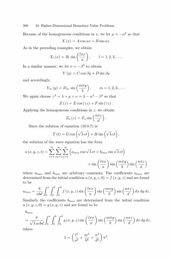
380 10 Higher-Dimensional Boundary-Value Problems
Because of the homogeneous conditions in x, we let µ = −α2 so that
X (x) = A cos αx + B sin αx.
As in the preceding examples, we obtain
Xl (x) = Bl sin(
lπx
a
), l = 1, 2, 3, . . . .
In a similar manner, we let ν = −β2 to obtain
Y (y) = C cos βy + D sin βy
and accordingly,
Ym (y) = Dm sin(mπy
b
), m = 1, 2, 3, . . . .
We again choose γ2 = λ + µ + ν = λ − α2 − β2 so that
Z (z) = E cos (γz) + F sin (γz) .
Applying the homogeneous conditions in z, we obtain
Zn (z) = Fn sin(nπz
d
).
Since the solution of equation (10.8.7) is
T (t) = G cos(√
λ ct)
+ H sin(√
λ ct)
,
the solution of the wave equation has the form
u (x, y, z, t) =∞∑
l=1
∞∑m=1
∞∑n=1
(almn cos
√λ ct + blmn sin
√λ ct
)× sin
(lπx
a
)sin
(mπy
b
)sin
(nπz
d
)where almn and blmn are arbitrary constants. The coefficients almn aredetermined from the initial condition u (x, y, z, 0) = f (x, y, z) and are foundto be
almn =8
abd
∫ a
0
∫ b
0
∫ d
0f (x, y, z) sin
(lπx
a
)sin
(mπy
b
)sin
(nπz
d
)dx dy dz.
Similarly the coefficients blmn are determined from the initial conditionu (x, y, z, 0) = g (x, y, z) and are found to be
blmn
=8√
λ acbd
∫ a
0
∫ b
0
∫ d
0g (x, y, z) sin
(lπx
a
)sin
(mπy
b
)sin
(nπz
d
)dx dy dz,
where
λ =(
l2
a2 +m2
b2 +n2
d2
)π2.

10.9 Heat Conduction in a Rectangular Volume 381
10.9 Heat Conduction in a Rectangular Volume
As in the case of the wave equation, the solution of the heat equation inthree spaces variables can be determined. Consider the problem of heatdistribution in a rectangular volume. The faces are maintained at zero de-gree temperature. The solid is initially heated so that the problem may bewritten as
ut = k ∇2u, 0 < x < a, 0 < y < b, 0 < z < d, t > 0,
u (x, y, z, 0) = f (x, y, z) , 0 ≤ x ≤ a, 0 ≤ y ≤ b, 0 ≤ z ≤ d,
u (0, y, z, t) = 0, u (a, y, z, t) = 0,u (x, 0, z, t) = 0, u (x, b, z, t) = 0,u (x, y, 0, t) = 0, u (x, y, d, t) = 0.
As before, the separable equations are
T ′ + λkT = 0, (10.9.1)∇2U + λU = 0. (10.9.2)
If we assume the solution U to be of the form
U (x, y, z) = X (x) Y (y) Z (z) ,
then the solution of the Helmholtz equation is
Ulmn (x, y, z) = BlDmFn sin(
lπx
a
)sin
(mπy
b
)sin
(nπz
d
).
Since the solution of equation (10.9.1) is
T (t) = Ge−λkt,
the solution of the heat equation takes the form
u (x, y, z, t) =∞∑
l=1
∞∑m=1
∞∑n=1
almn e−λkt sin(
lπx
a
)sin
(mπy
b
)sin
(nπz
d
),
where λ =[(
l2/a2)
+(m2/b2
)+
(n2/d2
)]π2 and almn are constants.
Application of the initial condition yields
almn =(
8abd
)∫ a
0
∫ b
0
∫ d
0f (x, y, z) sin
(lπx
a
)sin
(mπy
b
)sin
(nπz
d
)dx dy dz.

382 10 Higher-Dimensional Boundary-Value Problems
10.10 The Schrodinger Equation and the HydrogenAtom
In quantum mechanics, the Hamiltonian (or energy operator) is usuallydenoted by H and is defined by
H =p2
2M+ V (r) (10.10.1)
where p = (/i) ∇ = −i∇ is the momentum of a particle of mass M ,h = 2π is the Planck constant, and V (r) is the potential energy.
The physical state of a particle at time t is described as fully as possibleby the wave function Ψ (r, t). The probability of finding the particle atposition r = (x, y, z) within a finite volume dV = dx dy dz is∫∫∫
|Ψ |2 dx dy dz.
The particle must always be somewhere in the space, so the probability offinding the particle within the whole space is one, that is,∫ ∞
−∞
∫ ∞
−∞
∫ ∞
−∞|Ψ |2 dx dy dz = 1.
The time dependent Schrodinger equation for the function Ψ (r, t) is
i Ψt = HΨ, (10.10.2)
where H is explicitly given by
H = − 2
2M∇2 + V (r) . (10.10.3)
Given the potential V (r), the fundamental problem of quantum me-chanics is to obtain a solution of (10.10.2) which agrees with a given initialstate Ψ (r, 0).
For the stationary state solutions, we seek a solution of the form
Ψ (r, t) = f (t) ψ (r) .
Substituting this into (10.10.2) gives
df
dt+
iE
f = 0, (10.10.4)
Hψ (r) = Eψ (r) , (10.10.5)
where E is a separation constant and has the dimension of energy. Integra-tion of (10.10.4) gives

10.10 The Schrodinger Equation and the Hydrogen Atom 383
f (t) = A exp(
− iEt
), (10.10.6)
where A is an arbitrary constant.Equation (10.10.5) is called the time independent Schrodinger equation.
The great importance of this equation follows from the fact that the sepa-ration of variables gives not just some particular solution of (10.10.5), butgenerally yields all solutions of physical interest. If ψE (r) represents oneparticular solution of (10.10.5), then most general solutions of (10.10.2) canbe obtained by the principle of superposition of such particular solutions.In fact, the general solution is given by
ψ (r, t) =∑E
AE exp(
− iEt
)ψE (r) , (10.10.7)
where the summation is taken over all admissible values of E, and AE isan arbitrary constant to be determined from the initial conditions.
We now solve the eigenvalue problem for the Schrodinger equation forthe spherically symmetric potential so that V (r) = V (r). The equation forthe wave function ψ (r) is
∇2ψ +2M
2 [E − V (r)] ψ = 0, (10.10.8)
where ∇2 is the three-dimensional Laplacian.
To determine the wave function ψ, it is convenient to introduce sphericalpolar coordinates (r, θ, φ) so that equation (10.10.8) takes the form
1r2
∂
∂r
(r2 ∂ψ
∂r
)+
1r2 sin θ
∂
∂θ
(sin θ
∂ψ
∂θ
)+
1r2 sin2 θ
∂2ψ
∂φ2
+K [E − V (r)] ψ = 0, (10.10.9)
where K =(2M/
2), ψ ≡ ψ (r, θ, φ), 0 ≤ r < ∞, 0 ≤ θ ≤ π, and 0 ≤ φ ≤
2π.
We seek a nontrivial separable solution of the form
ψ = R (r) Y (θ, φ)
and then substitute into (10.10.9) to obtain the following equations
d
dr
(r2 dR
dr
)+
[K (E − V ) r2 − λ
]R = 0, (10.10.10)[
1sin θ
∂
∂θ
(sin θ
∂
∂θ
)+
1sin2 θ
∂2
∂φ2
]Y + λY = 0, (10.10.11)
where λ is a separation constant.

384 10 Higher-Dimensional Boundary-Value Problems
We first solve (10.10.11) by separation of variables through Y =Θ (θ) Φ (φ) so that the equation becomes
sin θd
dθ
(sin θ
dΘ
dθ
)+
(λ sin2 θ − m2)Θ = 0, (10.10.12)
d2Φ
dφ2 + m2Φ = 0, (10.10.13)
where m2 is a separation constant.
The general solution of (10.10.13) is
Φ = A eimφ + B e−imφ,
where A and B are arbitrary constants to be determined by the boundaryconditions on ψ (r, θ, φ) = R (r) Θ (θ) Φ (φ) which will now be formulated.
According to the fundamental postulate of quantum mechanics, thewave function for a particle without spin must have a definite value atevery point in space. Hence, we assume that ψ is a single-valued functionof position. In particular, ψ must have the same value whether the az-imuthal coordinate φ is given by φ or φ + 2π, that is, Φ (φ) = Φ (φ + 2π).Consequently, the solution for Φ has the form
Φ = C eimΦ, m = 0, + 1, + 2, . . . , (10.10.14)
where C is an arbitrary constant.In order to solve (10.10.12), it is convenient to change the variable x =
cos θ, Θ (θ) = u (x), −1 ≤ x ≤ 1 so that this equation becomes
d
dx
[(1 − x2) du
dx
]+
(λ − m2
1 − x2
)u = 0. (10.10.15)
For the particular case m = 0, this equation becomes
d
dx
[(1 − x2) du
dx
]+ λu = 0. (10.10.16)
This is known as the Legendre equation, which gives the Legendre poly-nomials Pl (x) of degree l as solutions provided λ = l (l + 1) where l is apositive integer or zero.
When m = 0, equation (10.10.15) with λ = l (l + 1) admits solutionswhich are well known as associated Legendre functions, Pm
l (x) of degree land order m defined by
Pml (x) =
(1 − x2)m/2 dm
dxmPm
l (x) , x = cos θ.
Clearly, Pml (x) vanishes when m > l. As for the negative integral values of
m, it can be readily shown that

10.10 The Schrodinger Equation and the Hydrogen Atom 385
P−ml (x) = (−1)m (l − m)!
(l + m)!Pm
l (x) .
Hence, the functions P−ml (x) differ from Pm
l (x) by a constant factor, andas a consequence, m is restricted to a positive integer or zero. Thus, theassociated Legendre functions Pm
l (x) with |m| ≤ l are the only nonsingularand physically acceptable solutions of (10.10.15). Since |m| ≤ l, when l = 0,m = 0; when l = 1, m = −1, 0, +1; when l = 2, m = −2, −1, 0, 1, 2,etc. This means that, given l, there are exactly (2l + 1) different values ofm = −l, . . ., −1, 0, 1,. . ., l. The numbers l and m are called the orbitalquantum member and the magnetic quantum number respectively.
It is convenient to write down the solutions of (10.10.11) as functionswhich are normalized with respect to an integration over the whole solidangle. They are called spherical harmonics and are given by, for m ≥ 0,
Y ml (θ, φ) =
[(2l + 1)
4π
(l − m)!(l + m)!
] 12
(−1)meimφPm
l (cos θ) . (10.10.17)
Spherical harmonics with negative m and with |m| ≤ l are defined by
Y ml (θ, φ) = (−1)m
Y −ml (θ, φ). (10.10.18)
We now return to a general discussion of the radial equation (10.10.10)which becomes, under the transformation R (r) = P (r) /r,
d2P
dr2 +[K (E − V ) − λ
r2
]P (r) = 0. (10.10.19)
Almost all cases of physical interest require V (r) to be finite everywhereexcept at the origin r = 0. Also, V (r) → 0 as r → ∞. The Coulomb andsquare well potentials are typical examples of this kind. In the neighborhoodof r = 0, V (r) can be neglected compared to the centrifugal term
(∼ 1/r2)
so that equation (10.10.19) takes the form
d2P
dr2 − l (l + 1)r2 P (r) = 0 (10.10.20)
for all states with l = 0. The general solution of this equation is
P (r) = A rl+1 + B r−l, (10.10.21)
where A and B are arbitrary constants. With the boundary conditionP (0) = 0, B = 0 so that the solution is proportional to rl+1.
On the other hand, in view of the assumption that V (r) → 0 as r → ∞,the radial equation (10.10.19) reduces to
d2P
dr2 + KE P (r) = 0. (10.10.22)

386 10 Higher-Dimensional Boundary-Value Problems
The general solution of this equation is
P (r) = C eir√
KE + D e−ir√
KE . (10.10.23)
The solution is oscillatory for E > 0, and exponential in nature for E < 0.The oscillatory solutions are not physically acceptable because the wavefunction does not tend to zero as r → ∞. When E < 0, the second termin (10.10.23) tends to infinity as r → ∞. Consequently, the only physicallyacceptable solutions for E > 0, have the asymptotic form
P (r) = C e−αr/2, (10.10.24)
where KE = − (α2/4
).
Thus, the general solution of (10.10.19) can be written as
P (r) = f (r) e−(α/2)r,
so that f (r) satisfies the ordinary differential equation
d2f
dr2 − αdf
dr−
[KV +
l (l + 1)r2
]f = 0. (10.10.25)
Note that this general solution is physically acceptable because the wavefunction tends to zero as r → 0 and as r → ∞.
We now specify the form of the potential V (r). One of the most com-mon potentials is the Coulomb potential V (r) = −Ze2/r representing theattraction between an atomic nucleus of charge +Ze and a moving electronof charge −e. For the hydrogen atom Z = 1. It is a two particle system con-sisting of a negatively charged electron interacting with a positively chargedproton. On the other hand, a helium atom consists of two protons and twoneutrons. There are two electrons in orbit around the nucleus of a heliumatom. For the singly charged helium ion Z = 2, where Z represents thenumber of unit charges of the nucleus. Consequently, equation (10.10.25)reduces to
d2f
dr2 − αdf
dr+
[KZe2
r− l (l + 1)
r2
]f (r) = 0. (10.10.26)
We seek a power series solution of this equation in the form
f (r) = rk∞∑
s=1
asrs, k = 0. (10.10.27)
Substituting this series into (10.10.26), we obtain
rk∞∑
s=1
[(s + k) (s + k − 1) − l (l + 1)] asrs+k−1
+∞∑
s=1
[Zke2 − α (s + k)
]asr
s+k−1 = 0.

10.10 The Schrodinger Equation and the Hydrogen Atom 387
Clearly, the lowest power of r is (k − 1), so that
[k (k + 1) − l (l + 1)] a1 = 0.
This implies that k = l or − (l + 1) provided a1 = 0. The negative root of kis not acceptable because it leads to an unbounded solution. Equating thecoefficient of rs+k−1, we get the recurrence relation for the coefficients as
as+1 =α (s + l) − ZKe2
s (s + 2l + 1)as, s = 1, 2, 3, . . . . (10.10.28)
The asymptotic nature of this result is
as+1
as∼ α
sas s → ∞.
This ratio is the same as that of the series for eαr. This means that R (r) isunbounded as r → ∞, which is physically unacceptable. Hence, the seriesfor f (r) must terminate, and f (r) must be a polynomial so that as+1 = 0,but as = 0. Hence
α (s + l) − ZKe2 = 0, s = 1, 2, 3, . . . ,
or,
α2
4=
Z2K2e4
4 (s + l)2= −KE. (10.10.29)
Putting K =(2M/
2), the energy levels are given by
E = En = −Z2K2e4
4n2K= −MZ2e4
22n2 , (10.10.30)
where n = (s + l) is called the principal quantum number and n = 1, 2, 3, . . ..Thus, it turns out that the complete solution of the Schrodinger equation
is given by
ψn,l,m (r, θ, φ) = Rn,l (r) Y ml (θ, φ) ,
where the radial part is the solution of the radial equation (10.10.10), andit depends on the principle quantum number n (energy levels) and theorbital quantum number l. However, it does not depend on the magneticquantum number m. Of course, there are (2l + 1) states with the same lvalue but with different m values. Each of these states has the same energy,and therefore, such systems have a (2l + 1)-fold degeneracy, as a result ofrotational symmetry.
For the hydrogen atom, Z = 1, the discrete energy spectrum is
En = − Me4
22n2 = − e2
2an2 , (10.10.31)

388 10 Higher-Dimensional Boundary-Value Problems
where a =(
2/e2M)
is called the Bohr radius of the hydrogen atom ofmass M and charge of the electron, −e. This discrete energy spectrumdepends only on the principle quantum number n (but not on m) and hasan excellent agreement with experimental prediction of spectral lines.
For a given n, there are n sets of l and s
n = 1, l = 0, s = 1 ; n = 2,
⎧⎨⎩l = 0, s = 2
l = 1, s = 1
⎫⎬⎭ ;
n = 3,
⎧⎪⎪⎪⎪⎨⎪⎪⎪⎪⎩l = 0, s = 3
l = 1, s = 2
l = 2, s = 1
⎫⎪⎪⎪⎪⎬⎪⎪⎪⎪⎭ ; etc.
Given n, there are exactly n values of l (l = 0, 1, 2, . . . , n − 1) and thehighest value of l is n − 1.
Thus, the three numbers n, l, m, determine a unique eigenfunction,ψn,l,m (r, θ, φ) = Rn,l (r) Y m
l (θ, φ). Since the energy levels depend only onthe principle quantum number n, there are, in general, several linearly inde-pendent eigenfunctions of the Schrodinger equation for the hydrogen atomcorresponding to each energy level, so the energy levels are said to be de-generate. There are (2l + 1) different eigenfunctions of the same energyobtained by varying the magnetic quantum number m from −l to l. Ingeneral, the total number of degenerate energy states En for the hydrogenatom is then
n−1∑l=0
(2l + 1) = 2n (n − 1)
2+ n = n2. (10.10.32)
The energy levels of the hydrogen atom (10.10.31) can be expressed interms the Rydberg, Ry, as
En = −Ry
n2 , (10.10.33)
where Ry represents the Rydberg given by
Ry =Me4
22 =Mc2e4
2 (c)2=
Mc2
2×
(e2
c
)2
5 × 10⁵
2eV ×
(1
137
)2
13.3 eV.
Consequently,
En = −13.3n2 eV. (10.10.34)

10.10 The Schrodinger Equation and the Hydrogen Atom 389
Thus, the ground state of the hydrogen atom, which is the most tightlybound, has an energy −13.3 eV (more accurately −13.6 eV ) and therefore, itwould take 13.6 eV to release the electron from its ground state. Therefore,this is called the binding energy of the hydrogen atom.
Finally, the electron is treated here as a nonrelativistic particle. How-ever, in reality, small relativistic effects can be calculated. These are knownas fine structure corrections. Thus, the nonrelativistic Schrodinger equationdescribes the hydrogen atom extremely well.
Example 10.10.1. (Infinite Square well potential V0 → ∞). We considerthe one-dimensional Schrodinger equation (10.10.8) in the form[
−(
2
2M
)d2
dx2 + V (x)]
ψ (x) = Eψ (x) , (10.10.35)
where the potential V (x) is given by
V (x) =
⎧⎨⎩V0, x ≤ −a, x ≥ a,
0, −a ≤ x ≤ a(10.10.36)
and take the limit V0 → +∞ as shown in Figure 10.10.1.It is noted that the potential is zero inside the square well and E is
the kinetic energy of the particle in this region (−a ≤ x ≤ a) which mustbe positive, E > 0. It is convenient to fix the origin at the center of thewell so that V (x) is an even function of x. A case of special interest is thatV0 > E ≥ 0 and eventually, V0 → ∞.
Figure 10.10.1 Square well with potential V0 → ∞.

390 10 Higher-Dimensional Boundary-Value Problems
The given potential is different in different regions, we solve (10.10.35)separately in three regions.
Region 1. V = V0 in this region x ≤ −a.
The Schrodinger equation (10.10.35) in this region is
− 2
2Mψxx + V0ψ = Eψ.
Or, equivalently,
ψxx =(
2M
2
)(V0 − E) ψ, V0 > E > 0. (10.10.37)
The general solution of (10.10.37) is
ψ1 (x) = A ekx + B e−kx, (10.10.38)
where A and B are constants and
k =[2M
2 (V0 − E)] 1
2
. (10.10.39)
The wave function ψ1 (x) must be bounded as x → −∞ to retain its prob-abilistic interpretation, hence B = 0, and the solution in x ≤ −a is
ψ1 (x) = A ekx.
As V0 → ∞, k → ∞, and, in this limit, the solution must vanish, that is,
ψ1 (x) = 0, for x ≤ −a. (10.10.40)
Region 2. V = 0 in −a ≤ x ≤ a.In this case, the equation takes the form
ψxx + k2ψ = 0, (10.10.41)
where
k2 =2ME
2 . (10.10.42)
The general solution of (10.10.41) is given by
ψ2 (x) = C sin kx + D cos kx, (10.10.43)
where C and D are arbitrary constants.Region 3. V = V0 in this region x ≥ a.An argument similar to region 1 leads to zero solution, that is,
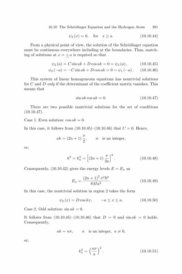
10.10 The Schrodinger Equation and the Hydrogen Atom 391
ψ3 (x) = 0, for x ≥ a. (10.10.44)
From a physical point of view, the solution of the Schrodinger equationmust be continuous everywhere including at the boundaries. Thus, match-ing of solutions at x = + a is required so that
ψ2 (a) = C sin ak + D cos ak = 0 = ψ3 (a) , (10.10.45)ψ2 (−a) = −C sin ak + D cos ak = 0 = ψ1 (−a) . (10.10.46)
This system of linear homogeneous equations has nontrivial solutionsfor C and D only if the determinant of the coefficient matrix vanishes. Thismeans that
sin ak cos ak = 0. (10.10.47)
There are two possible nontrivial solutions for the set of conditions(10.10.47).
Case 1. Even solution: cos ak = 0.
In this case, it follows from (10.10.45)–(10.10.46) that C = 0. Hence,
ak = (2n + 1)π
2, n is an integer,
or,
k2 = k2n =
[(2n + 1)
π
2a
]2. (10.10.48)
Consequently, (10.10.42) gives the energy levels E = En as
En =(2n + 1)2 π2
2
8Ma2 . (10.10.49)
In this case, the nontrivial solution in region 2 takes the form
ψ2 (x) = D cos kx, −a ≤ x ≤ a. (10.10.50)
Case 2. Odd solution: sin ak = 0.
It follows from (10.10.45)–(10.10.46) that D = 0 and sin ak = 0 holds.Consequently,
ak = nπ, n is an integer, n = 0,
or,
k2n =
(nπ
a
)2. (10.10.51)

392 10 Higher-Dimensional Boundary-Value Problems
Thus, the energy levels are given by
En =
2k2n
2M=
(nπ)2
2Ma2 . (10.10.52)
The nontrivial solution in region 2 is
ψ2 (x) = C sin kx, −a ≤ x ≤ a. (10.10.53)
Thus, it turns out that, corresponding to every value of En given by(10.10.49) or (10.10.52), there exists a physically acceptable solution. Hence,the general solution of the Schrodinger equation is obtained from (10.10.7)in the form
ψ (x, t) =∑
n
Cnψn (x) exp(
− itEn
), (10.10.54)
where Cn are constants.In classical mechanics, the motion of the particle is allowed for E > 0.
In quantum mechanics, it follows from (10.10.49) or (10.10.52) that particlemotion is allowed for discrete values of energy, that is, the energy for thissystem is quantized. This is a remarkable contrast between the results ofthe classical mechanics and quantum mechanics.
Finally, it follows from the above analysis is that
lim|x|→∞
ψ (x) = 0. (10.10.55)
Such a system, where the wave function vanishes beyond range or asymp-totically, is called a bound state, and energy is quantized. A very commonexample is the hydrogen atom which was discussed in this section. In thepresent system ψ (x) = 0 for x2 ≥ a2. Therefore, this system is also referredto as a particle in a box of length 2a. The probability for finding the particleoutside this region is zero.
10.11 Method of Eigenfunctions and Vibration ofMembrane
Consider the nonhomogeneous initial boundary-value problem
L [u] = ρ utt − G in D (10.11.1)
with prescribed homogeneous boundary conditions on the boundary B ofD, and the initial conditions
u (x1, x2, . . . , xn, 0) = f (x1, x2, . . . , xn) , (10.11.2)ut (x1, x2, . . . , xn, 0) = g (x1, x2, . . . , xn) . (10.11.3)

10.11 Method of Eigenfunctions and Vibration of Membrane 393
Here ρ ≡ ρ (x1, x2, . . . , xn) is a real-valued positive continuous function andG ≡ G (x1, x2, . . . , xn) is a real-valued continuous function.
We assume that the only solution of the associated homogeneous prob-lem
L [u] = ρutt (10.11.4)
with the prescribed boundary conditions is the trivial solution. Then, ifthere exists a solution of the given problem (10.11.1)–(10.11.3), it can berepresented by a series of eigenfunctions of the associated eigenvalue prob-lem
L [ϕ] + λ ρ ϕ = 0 (10.11.5)
with ϕ satisfying the boundary conditions given for u. For problems withone space variable, see Section 7.8.
As a specific example, we shall determine the solution of the problem offorced vibration of a rectangular membrane of length a and width b. Theproblem is
utt − c2∇2u = F (x, y, t) in D (10.11.6)u (x, y, 0) = f (x, y) , 0 ≤ x ≤ a, 0 ≤ y ≤ b, (10.11.7)
ut (x, y, 0) = g (x, y) , 0 ≤ x ≤ a, 0 ≤ y ≤ b, (10.11.8)u (0, y, t) = 0, u (a, y, t) = 0, (10.11.9)u (x, 0, t) = 0, u (x, b, t) = 0. (10.11.10)
The associated eigenvalue problem is
∇2ϕ + λϕ = 0 in D,
ϕ = 0 on the boundary B of D.
The eigenvalues for this problem according to Section 10.6 are given by
αmn =(
m2π2
a2 +n2π2
b2
), m, n = 1, 2, 3 . . .
and the corresponding eigenfunctions are
ϕmn (x, y) = sin(mπx
a
)sin
(nπy
b
).
Thus, we assume the solution
u (x, y, t) =∞∑
m=1
∞∑n=1
umn (t) sin(mπx
a
)sin
(nπy
b
)and the forcing function

394 10 Higher-Dimensional Boundary-Value Problems
F (x, y, t) =∞∑
m=1
∞∑n=1
Fmn (t) sin(mπx
a
)sin
(nπy
b
).
Here Fmn (t) are given by
Fmn (t) =4ab
∫ a
0
∫ b
0F (x, y, t) sin
(mπx
a
)sin
(nπy
b
)dx dy.
Note that u automatically satisfies the homogeneous boundary conditions.Now inserting u (x, y, t) and F (x, y, t) in equation (10.11.6), we obtain
umn + c2α2mnumn = Fmn,
where α2mn = (mπ/a)2 + (nπ/b)2. We have assumed that u is twice contin-
uously differentiable with respect to t. Thus, the solution of the precedingordinary differential equation takes the form
umn (t) = Amn cos (αmnct) + Bmn sin (αmnct)
+1
(αmn c)
∫ t
0Fmn (τ) sin [αmnc (t − τ)] dτ.
The first initial condition gives
u (x, y, 0) = f (x, y) =∞∑
m=1
∞∑n=1
Amn sin(mπx
a
)sin
(nπy
b
).
Assuming that f (x, y) is continuous in x and y, the coefficient Amn of thedouble Fourier series is given by
Amn =4ab
∫ a
0
∫ b
0f (x, y) sin
(mπx
a
)sin
(nπy
b
)dx dy.
Similarly, from the remaining initial condition, we have
ut (x, y, 0) = g (x, y) =∞∑
m=1
∞∑n=1
Bmn (αmn c) sin(mπx
a
)sin
(nπy
b
),
and hence, for continuous g (x, y),
Bmn =4
(ab αmnc)
∫ a
0
∫ b
0g (x, y) sin
(mπx
a
)sin
(nπy
b
)dx dy.
The solution of the given initial boundary-value problem is therefore givenby
u (x, y, t) =∞∑
m=1
∞∑n=1
umn (t) sin(mπx
a
)sin
(nπy
b
),

10.12 Time-Dependent Boundary-Value Problems 395
provided the series for u and its first and second derivatives converge uni-formly.
If F (x, y, t) = ex+y cos ωt, then
Fmn (t) =4mnπ2
(m2π2 + a2) (n2π2 + b2)
[1 + (−1)m+1
ea]
×[1 + (−1)n+1
eb]cos ωt
= Cmn cos ωt.
Hence, we have
umn (t) =1
(αmnc)
∫ t
0Cmn cos ωt sin [αmnc (t − τ)] dτ
=Cmn
(α2mnc2 − ω2)
(cos ωt − cos αmnct)
provided ω = (αmnc). Thus, the solution may be written in the form
u (x, y, t) =∞∑
m=1
∞∑n=1
Cmn
(α2mnc2 − ω2)
(cos ωt − cos αmnct)
× sin(mπx
a
)sin
(nπy
b
).
10.12 Time-Dependent Boundary-Value Problems
The preceding chapters have been devoted to problems with homogeneousboundary conditions. Due to the frequent occurrence of problems with timedependent boundary conditions in practice, we consider the forced vibrationof a rectangular membrane with moving boundaries. The problem here isto determine the displacement function u which satisfies
utt − c2∇2u = F (x, y, t) , 0 < x < a, 0 < y < b, (10.12.1)u (x, y, 0) = f (x, y) , 0 ≤ x ≤ a, 0 ≤ y ≤ b, (10.12.2)
ut (x, y, 0) = g (x, y) , 0 ≤ x ≤ a, 0 ≤ y ≤ b, (10.12.3)u (0, y, t) = p1 (y, t) , 0 ≤ y ≤ b, t ≥ 0, (10.12.4)u (a, y, t) = p2 (y, t) , 0 ≤ y ≤ b, t ≥ 0, (10.12.5)u (x, 0, t) = q1 (x, t) , 0 ≤ x ≤ a, t ≥ 0, (10.12.6)u (x, b, t) = q2 (x, t) , 0 ≤ x ≤ a, t ≥ 0. (10.12.7)
For such problems, we seek a solution in the form
u (x, y, t) = U (x, y, t) + v (x, y, t) , (10.12.8)

396 10 Higher-Dimensional Boundary-Value Problems
where v is the new dependent variable to be determined. Before finding v,we must first determine U . If we substitute equation (10.12.8) into equations(10.12.1)–(10.12.7), we respectively obtain
vtt − c2 (vxx + vyy) = F − Utt + c2 (Uxx + Uyy) = F (x, y, t)
and
v (x, y, 0) = f (x, y) − U (x, y, 0) = f (x, y) ,
vt (x, y, 0) = g (x, y) − Ut (x, y, 0) = g (x, y) ,
v (0, y, t) = p1 (y, t) − U (0, y, t) = p1 (y, t) ,
v (a, y, t) = p2 (y, t) − U (a, y, t) = p2 (y, t) ,
v (x, 0, t) = q1 (x, t) − U (x, 0, t) = q1 (x, t) ,
v (x, b, t) = q2 (x, t) − U (x, b, t) = q2 (x, t) .
In order to make the conditions on v homogeneous, we set
p1 = p2 = q1 = q2 = 0,
so that
U (0, y, t) = p1 (y, t) , U (a, y, t) = p2 (y, t) , (10.12.9)U (x, 0, t) = q1 (x, t) , U (x, b, t) = q2 (x, t) . (10.12.10)
In order that the boundary conditions be compatible, we assume that theprescribed functions take the forms
p1 (y, t) = ϕ (y) p∗1 (y, t) , p2 (y, t) = ϕ (y) p∗
2 (y, t) ,
q1 (x, t) = ψ (x) q∗1 (x, t) , q2 (x, t) = ψ (x) q∗
2 (x, t) ,
where the function ϕ must vanish at the end points y = 0, y = b and thefunction ψ must vanish at x = 0, x = a. Thus, U (x, y, t) which satisfiesequations (10.12.9)–(10.12.10) takes the form
U (x, y, t) = ϕ (y)[p∗1 +
x
a(p∗
2 + p∗1)
]+ ψ (x)
[q∗1 +
y
b(q∗
2 + q∗1)
].
The problem then is to find the function v (x, y, t) which satisfies
vtt − c2 (vxx + vyy) = F (x, y, t) ,
v (x, y, 0) = f (x, y) , vt (x, y, 0) = g (x, y) ,
v (0, y, t) = 0, v (a, y, t) = 0,v (x, 0, t) = 0, v (x, b, t) = 0.
This is an initial boundary-value problem with homogeneous boundary con-ditions, which has already been solved.

10.12 Time-Dependent Boundary-Value Problems 397
As a particular case, consider the following problem
utt − c2 (uxx + uyy) = 0,
u (x, y, 0) = 0, ut (x, y, 0) =y
bsin
(πx
a
),
u (0, y, t) = 0, u (a, y, t) = 0,
u (x, 0, t) = 0, u (x, b, t) = sin(πx
a
)sin t.
We assume a solution in the form
u (x, y, t) = v (x, y, t) + U (x, y, t) .
The function U (x, y, t) which satisfies
U (0, y, t) = 0, U (a, y, t) = 0,
U (x, 0, t) = 0, U (x, b, t) = sin(πx
a
)sin t
is
U (x, y, t) = sin(πx
a
)(y
bsin t
).
Thus, the new problem to be solved is
vtt − c2 (vxx + vyy) =(
1 − c2π2
a2
)y
bsin
(πx
a
)sin t,
v (x, y, 0) = 0, vt (x, y, 0) = 0,v (0, y, t) = 0, v (a, y, t) = 0,v (x, 0, t) = 0, v (x, b, t) = 0.
Then, we find Fmn from
Fmn (t) =4ab
∫ a
0
∫ b
0F (x, y, t) sin
(mπx
a
)sin
(nπy
b
)dx dy,
where
F (x, y, t) =(
1 − c2π2
a2
)y
bsin
(πx
a
)sin t,
and obtain
Fmn (t) =2 (−1)n+1
an
(1 − c2π2
a2
)sin t.
Now we determine vmn (t) which are given by

398 10 Higher-Dimensional Boundary-Value Problems
vmn (t) = Amn cos (αmnct) + Bmn sin (αmnct)
+1
αmnc
∫ t
0Fmn (τ) sin [αmnc (t − τ)] dτ.
Since v (x, y, 0) = 0, Amn = 0, but
Bmn =4
ab αmnc
∫ a
0
∫ b
0
(−y
bsin
πx
a
)sin
(mπx
a
)sin
(nπy
b
)dx dy
=2 (−1)n
αmnnac.
Thus, we have
vmn (t) =2 (−1)n
αmnnacsin (αmnct)
+2 (−1)n
αmnca3n (1 − α2c2)(a2 − c2π2) (sin αmnct − αc sin t) .
The solution is therefore given by
u (x, y, t) =y
bsin
(πx
a
)sin t +
∞∑m=1
∞∑n=1
vmn (t) sin(mπx
a
)sin
(nπy
b
).
10.13 Exercises
1. Solve the Dirichlet problem
∇2u = 0, 0 < x < a, 0 < y < b, 0 < z < c,
u (0, y, z) = sin(πy
b
)sin
(πz
c
), u (a, y, z) = 0,
u (x, 0, z) = 0, u (x, b, z) = 0,u (x, y, 0) = 0, u (x, y, c) = 0.
2. Solve the Neumann problem
∇2u = 0, 0 < x < 1, 0 < y < 1, 0 < z < 1,
ux (0, y, z) = 0, ux (1, y, z) = 0,uy (x, 0, z) = 0, uy (x, 1, z) = 0,uz (x, y, 0) = cos πx cos πy, uz (x, y, 1) = 0.
3. Solve the Robin boundary-value problem
∇2u = 0, 0 < x < π, 0 < y < π, 0 < z < π,
u (0, y, z) = f (y, z) , u (π, y, z) = 0,uy (x, 0, z) = 0, uy (x, π, z) = 0,
uz (x, y, 0) + hu (x, y, 0)
uz (x, y, π) + hu (x, y, π)
=
=
0,
0,
⎫⎬⎭ h = constant.

10.13 Exercises 399
4. Determine the solution of each of the following problems for a cylinder:
(a) ∇2u = 0, r < a, 0 < θ < 2π, 0 < z < l,
u (a, θ, z) = 0, u (r, θ, l) = 0, u (r, θ, 0) = f (r, θ) .
(b) ∇2u = 0, r < a, 0 < θ < 2π, 0 < z < l,
u (a, θ, z) = f (θ, z) , uz (r, θ, 0) = 0, uz (r, θ, l) = 0.
5. Find the solution of the Dirichlet problem for a sphere
∇2u = 0, r < a, 0 < θ < π, 0 < ϕ < 2π,
u (a, θ, ϕ) = cos2 θ.
6. Solve the Dirichlet problem in a region bounded by two concentricspheres
∇2u = 0, a < r < b, 0 < θ < π, 0 < φ < 2π,
u (a, θ, φ) = f (θ, φ) , u (b, θ, φ) = g (θ, φ) .
7. Find the steady-state temperature distribution in a cylinder of radiusa if a constant flow of heat T is supplied at the end z = 0, and thesurface r = a and the end z = l are maintained at zero temperature.
8. Find the potential of the electrostatic field inside a cylinder of length land radius a, if each end of the cylinder is grounded, and the surface ischarged to a potential u0.
9. Determine the potential of the electric field inside a sphere of radiusa, if the upper half of the sphere is charged to a potential u1 and thelower half to a potential u2.
10. Solve the Dirichlet problem for a half cylinder
∇2u = 0, r < 1, 0 < θ < π, 0 < z < 1,
u (1, θ, z) = 0, u (r, 0, z) = 0, u (r, π, z) = 0,
u (r, θ, 0) = 0, u (r, θ, 1) = f (r, θ) .
11. Solve the Neumann problem for a sphere

400 10 Higher-Dimensional Boundary-Value Problems
∇2u = 0, r < 1, 0 < θ < π, 0 < ϕ < 2π,
ur (1, θ, ϕ) = f (θ, ϕ) ,
where ∫ 2π
0
∫ π
0f (θ, ϕ) sin θ dθ dϕ = 0.
12. Find the solution of the initial boundary-value problem
utt = c2∇2u, 0 < x < 1, 0 < y < 1, t > 0,
u (x, y, 0) = sin2 πx sin πy, ut (x, y, 0) = 0, 0 ≤ x ≤ 1, 0 ≤ y ≤ 1,
u (0, y, t) = 0, u (1, y, t) = 0, 0 ≤ y ≤ 1, t > 0,
u (x, 0, t) = 0, u (x, 1, t) = 0, 0 ≤ x ≤ 1, t > 0.
13. Obtain the solution of the problem
utt = c2∇2u, r < a, 0 < θ < 2π, t > 0,
u (r, θ, 0) = f (r, θ) , ut (r, θ, 0) = g (r, θ) , u (a, θ, t) = 0.
14. Determine the temperature distribution in a rectangular plate with ra-diation from its surface. The temperature distribution is described by
ut = k (uxx + uyy) − h (u − u0) , 0 < x < a, 0 < y < b, t > 0,
u (x, y, 0) = f (x, y) ,
u (0, y, t) = 0, u (a, y, t) = 0,u (x, 0, t) = 0, u (x, b, t) = 0,
where k, h and u0 are constants.
15. Solve the heat conduction problem in a circular plate
ut = k
(urr +
1r
ur +1r2 uθθ
), r < 1, 0 < θ < 2π, t > 0,
u (r, θ, 0) = f (r, θ) , u (1, θ, t) = 0.
16. Solve the initial boundary-value problem
utt = c2∇2u, 0 < x < 1, 0 < y < 1, 0 < z < 1, t > 0,
u (x, y, z, 0) = sinπx sin πy sin πz,

10.13 Exercises 401
ut (x, y, z, 0) = 0,
u (0, y, z, t) = u (1, y, z, t) = 0,
u (x, 0, z, t) = u (x, 1, z, t) = 0,
u (x, y, 0, t) = u (x, y, 1, t) = 0.
17. Solve
utt + k ut = c2∇2u, 0 < x < a, 0 < y < b, 0 < z < d, t > 0,
u (x, y, z, 0) = f (x, y, z) , ut (x, y, z, 0) = g (x, y, z) ,
u (0, y, z, t) = u (a, y, z, t) = 0,
u (x, 0, z, t) = u (x, b, z, t) = 0,
u (x, y, 0, t) = u (x, y, d, t) = 0.
18. Obtain the solution of the problem for t > 0,
utt = c2(
urr +1r
ur +1r2 uθθ + uzz
), r < a, 0 < θ < 2π, 0 < z < l,
u (r, θ, z, 0) = f (r, θ, z) , ut (r, θ, z, 0) = g (r, θ, z) ,
u (a, θ, z, t) = 0, u (r, θ, 0, t) = u (r, θ, l, t) = 0.
19. Determine the solution of the heat conduction problem
ut = k ∇2u, 0 < x < a, 0 < y < b, 0 < z < c, t > 0,
u (x, y, z, 0) = f (x, y, z) ,
ux (0, y, z, t) = ux (a, y, z, t) = 0,
uy (x, 0, z, t) = uy (x, b, z, t) = 0,
uz (x, y, 0, t) = uz (x, y, c, t) = 0.

402 10 Higher-Dimensional Boundary-Value Problems
20. Solve the problem
ut = k ∇2u, r < a, 0 < θ < 2π, 0 < z < l, t > 0,
u (r, θ, z, 0) = f (r, θ, z) ,
ur (a, θ, z, t) = 0,
u (r, θ, 0, t) = u (r, θ, l, t) = 0.
21. Find the temperature distribution in the section of a sphere cut outby the cone θ = θ0. The surface temperature is zero while the initialtemperature is given by f (r, θ, ϕ).
22. Solve the initial boundary-value problem
utt = c2∇2u + F (x, y, t) , 0 < x < a, 0 < y < b, t > 0,
u (x, y, 0) = f (x, y) , ut (x, y, 0) = g (x, y) ,
ux (0, y, t) = ux (a, y, t) = 0 for all t > 0,
uy (x, 0, t) = uy (x, b, t) = 0 for all t > 0.
23. Solve the problem
utt = c2∇2u + xy sin t, 0 < x < π, 0 < y < π, t > 0,
u (x, y, 0) = 0, ut (x, y, 0) = 0,
u (0, y, t) = u (π, y, t) = 0,
u (x, 0, t) = u (x, π, t) = 0.
24. Solve
ut = k∇2u + F (x, y, z, t) , 0 < x < a, 0 < y < b, 0 < z < c,
t > 0,
u (x, y, z, 0) = f (x, y, z) ,
u (0, y, z, t) = u (a, y, z, t) = 0,

10.13 Exercises 403
u (x, 0, z, t) = u (x, b, z, t) = 0,
uz (x, y, 0, t) = uz (x, y, c, t) = 0.
25. Solve the nonhomogeneous diffusion problem
ut = k ∇2u + A, 0 < x < π, 0 < y < π, t > 0,
u (x, y, 0) = 0,
u (0, y, t) = u (π, y, t) = 0,
uy (x, 0, t) + u (x, 0, t) = 0,
uy (x, π, t) + u (x, π, t) = 0,
where k and A are constants.
26. Find the temperature distribution of the composite cylinder consistingof an inner cylinder 0 ≤ r ≤ r0 and an outer cylindrical tube r0 ≤ r ≤ a.The surface temperature is maintained at zero degrees, and the initialtemperature distribution is given by f (r, θ, z).
27. Solve the initial boundary-value problem
ut − c2∇2u = 0, 0 < x < π, 0 < y < π, t > 0,
u (x, y, 0) = 0,
u (0, y, t) = u (π, y, t) = 0,
u (x, 0, t) = x (x − π) sin t, u (x, π, t) = 0, 0 ≤ x ≤ π, t ≥ 0.
28. Solve the problem
utt = c2∇2u, r < a, 0 < θ < 2π, t > 0,
u (r, θ, 0) = f (r, θ) ,
ut (r, θ, 0) = g (r, θ) ,
u (a, θ, t) = p (θ, t) .

404 10 Higher-Dimensional Boundary-Value Problems
29. Solve
ut = c2∇2u, r < a, t > 0,
u (r, θ, 0) = f (r, θ) , ut (a, θ, t) = g (θ, t) , 0 < θ < π.
30. Determine the solution of the biharmonic equation
∇4u = q/D
with the boundary conditions
u (x, 0) = u (x, b) = 0,
u(−a
2, y
)= u
(a
2, y
)= 0,
uxx
(−a
2, y
)= uxx
(a
2, y
)= 0,
uyy (x, 0) = uyy (x, b) = 0,
where q is the load per unit area and D is the flexural rigidity of theplate. This is the problem of the deflection of a uniformly loaded plate,the sides of which are simply supported.
31. (a) Show that the solution of the one-dimensional Schrodinger equationfor a free particle of mass M
ψt =(
i
2M
)ψxx
is
ψ (x, t) =(
N
b
)exp
(− x2
2b2
), b =
(a2 +
it
M
) 12
,
where a is an integrating constant that can be determined from theinitial value of the wave function ψ (x, t), and N is also a constantthat can be determined from the normalization of the probability (wavefunction) of finding the particle.
(b) Show that the Gaussian probability density is
|ψ|2 = ψψ∗ =|N |2ac
exp(
−x2
c2
),
and its mean width is
δ =c√2, C =
(a2 +
2t2
M2a2
) 12
.
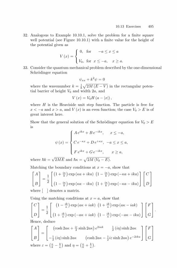
10.13 Exercises 405
32. Analogous to Example 10.10.1, solve the problem for a finite squarewell potential (see Figure 10.10.1) with a finite value for the height ofthe potential given as
V (x) =
⎧⎨⎩0, for −a ≤ x ≤ a
V0, for x ≤ −a, x ≥ a.
33. Consider the quantum mechanical problem described by the one-dimensionalSchrodinger equation
ψxx + k2ψ = 0
where the wavenumber k = 1
√2M (E − V ) in the rectangular poten-
tial barrier of height V0 and width 2a, and
V (x) = V0H (a − |x|) ,
where H is the Heaviside unit step function. The particle is free forx < −a and x > a, and V (x) is an even function; the case V0 > E is ofgreat interest here.
Show that the general solution of the Schrodinger equation for V0 > Eis
ψ (x) =
⎧⎪⎪⎪⎪⎨⎪⎪⎪⎪⎩A eikx + B e−ikx, x ≤ −a,
C e−κx + D e+κx, −a ≤ x ≤ a,
F eikx + Ge−ikx, x ≥ a,
where k =√
2ME and κ =√
2M (V0 − E).
Matching the boundary conditions at x = −a, show that⎡⎣A
B
⎤⎦ =12
⎡⎣(1 + iκ
k
)exp (κa + ika)
(1 − iκ
k
)exp (−κa + ika)(
1 − iκk
)exp (κa − ika)
(1 + iκ
k
)exp (−κa − ika)
⎤⎦⎡⎣C
D
⎤⎦where [ ] denotes a matrix.
Using the matching conditions at x = a, show that⎡⎣C
D
⎤⎦ =12
⎡⎣ (1 − ik
κ
)exp (aκ + iak)
(1 + ik
κ
)exp (aκ − iak)(
1 + ikκ
)exp (−aκ + iak)
(1 − ik
κ
)exp (−aκ − ika)
⎤⎦⎡⎣F
G
⎤⎦ .
Hence, deduce⎡⎣A
B
⎤⎦ =
⎡⎣ (cosh 2aκ + iε
2 sinh 2aκ)e2iak 1
2 (iη) sinh 2aκ
− 12 (iη) sinh 2aκ
(cosh 2aκ − 1
2 iε sinh 2aκ)e−2ika
⎤⎦⎡⎣F
G
⎤⎦where ε =
(κk − k
κ
)and η =
(κk + k
κ
).

11
Green’s Functions and Boundary-ValueProblems
“Potential theory has developed out of the vector analysis created by Gauss,Green, and Kelvin for the mathematical theories of gravitational attraction,of electrostatics and of the hydrodynamics of perfect fluids (i.e., incom-pressible and inviscid fluids). The first stage of abstraction was the studyof harmonic functions, i.e., potential functions in space free from masses,charges, sources, or sinks. This led to the inspired intuition of Dirichlet andthe early attempts to justify his ‘principle’.”
George Temple
11.1 Introduction
Boundary-value problems associated with either ordinary or partial dif-ferential equations arise most frequently in mathematics, mathematicalphysics and engineering science. The linear superposition principle is one ofthe most elegant and effective methods to represent solutions of boundary-value problems in terms of an auxiliary function known as Green’s function.Such a function was first introduced by George Green as early as 1828. Sub-sequently, the method of Green’s functions became a very useful analyticalmethod in mathematics and in many of the applied sciences.
In previous chapters, it has been shown that the eigenfunction methodcan effectively be used to express the solutions of differential equations asinfinite series. On the other hand, solutions of differential equations can beobtained as an integral superposition in terms of Green’s functions. So themethod of Green’s functions offers several advantages over eigenfunction ex-pansions. First, an integral representation of solutions provides a direct wayof describing the general analytical structure of a solution that may be ob-scured by an infinite series representation. Second, from an analytical pointof view, the evaluation of a solution from an integral representation mayprove simpler than finding the sum of an infinite series, particularly near

408 11 Green’s Functions and Boundary-Value Problems
rapidly-varying features of a function, where the convergence of an eigen-function expansion may be slow. Third, in view of the Gibbs phenomenondiscussed in Chapter 6, the integral representation seems to impose lessstringent requirements on the functions that describe the values that thesolution must assume on a given boundary than the expansion based oneigenfunctions.
Many physical problems are described by second-order nonhomogeneousdifferential equations with homogeneous boundary conditions or by second-order homogeneous equations with nonhomogeneous boundary conditions.Such problems can be solved by the method of Green’s functions.
We consider a nonhomogeneous partial differential equation of the form
Lxu (x) = f (x) , (11.1.1)
where x = (x, y, z) is a vector in three (or higher) dimensions, Lx is alinear partial differential operator in three or more independent variableswith constant coefficients, and u (x) and f (x) are functions of three ormore independent variables. The Green’s function G (x, ξ) of this problemsatisfies the equation
LxG (x, ξ) = δ (x − ξ) (11.1.2)
and represents the effect at the point x of the Dirac delta function sourceat the point ξ = (ξ, η, ζ).
Multiplying (11.1.2) by f (ξ) and integrating over the volume V of theξ space, so that dV = dξ dη dζ, we obtain∫
V
LxG (x, ξ) f (ξ) dξ =∫
V
δ (x − ξ) f (ξ) dξ = f (x) . (11.1.3)
Interchanging the order of the operator Lx and integral sign in (11.1.3)gives
Lx
[∫V
G (x, ξ) f (ξ) dξ
]= f (x) . (11.1.4)
A simple comparison of (11.1.4) with (11.1.1) leads to the solution of(11.1.1) in the form
u (x) =∫
V
G (x, ξ) f (ξ) dξ. (11.1.5)
Clearly, (11.1.5) is valid for any finite number of components of x. Ac-cordingly, the Green’s function method can be applied, in general, to anylinear, constant coefficient, nonhomogeneous partial differential equation inany number of independent variables.
Another way to approach the problem is by looking for the inverseoperator L−1
x . If it is possible to find L−1x , then the solution of (11.1.1) can

11.2 The Dirac Delta Function 409
be obtained as u (x) = L−1x (f (x)). It turns out that in many important
cases it is possible, and the inverse operator can be expressed as an integraloperator of the form
u (x) = L−1x (f (ξ)) =
∫V
G (x, ξ) f (ξ) dξ. (11.1.6)
The kernel G (x, ξ) is called the Green’s function which is, in fact, the char-acteristic of the operator Lx for any finite number of independent variables.
In our study of partial differential equations with the aid of Green’sfunctions, special attention will be given to those three partial differen-tial equations which occur most frequently in mathematics, mathematicalphysics and engineering science; the wave equation
utt − c2∇2u = f (x) , (11.1.7)
the heat or diffusion equation
ut − κ∇2u = f (x) , (11.1.8)
and the potential or the Laplace equation
∇2u = f (x) , (11.1.9)
where the Laplacian ∇2 in an n-dimensional Euclidean space is given by
∇2 ≡ ∂2
∂x21
+∂2
∂x22
+ . . . +∂2
∂x2n
, (11.1.10)
and x = (x1, x2, . . . , xn).Clearly, the solutions of the wave and heat equations are functions of
(n + 1) coordinates consisting of n space dimensions, x = (x1, x2, . . . , xn)and one time dimension t, whereas the solutions of the Laplace equationare functions of n space dimensions.
This chapter deals with the basic idea and properties of Green’s func-tions and how to construct such functions for finding solutions of partialdifferential equations. Some examples of applications are provided in thischapter and in the next chapter.
11.2 The Dirac Delta Function
The application of Green’s functions to boundary-value problems in ordi-nary differential equations was described earlier in Chapter 8. The Green’sfunction method is applied here to boundary-value problems in partial dif-ferential equations. The method provides solutions in integral form and isapplicable to a wide class of problems in applied mathematics and mathe-matical physics.
410 11 Green’s Functions and Boundary-Value Problems
Before developing the method of Green’s functions, we will first definethe Dirac delta function δ (x − ξ, y − η) in two dimensions by
(a) δ (x − ξ, y − η) = 0, x = ξ, y = η, (11.2.1)
(b)∫∫
Rε
δ (x − ξ, y − η) dx dy = 1, Rε : (x − ξ)2 + (y − η)2 < ε2,
(11.2.2)
(c)∫∫
R
F (x, y) δ (x − ξ, y − η) dx dy = F (ξ, η) , (11.2.3)
for arbitrary continuous function F in the region Rε.The delta function is not a function in the ordinary sense. For an elegant
treatment of the delta function as a generalized function, see L. Schwartz,Theorie des Distributions (1950, 1951). It is a symbolic function, and isoften viewed as the limit of a distribution.
If δ (x − ξ) and δ (y − η) are one-dimensional delta functions, we have∫∫R
F (x, y) δ (x − ξ) δ (y − η) dx dy = F (ξ, η) . (11.2.4)
Since (11.2.3) and (11.2.4) hold for an arbitrary continuous function F , weconclude that
δ (x − ξ, y − η) = δ (x − ξ) δ (y − η) . (11.2.5)
Thus, we may state that the two-dimensional delta function is the productof two one-dimensional delta functions.
Higher dimensional delta functions can be defined in a similar manner.
δ (x1, x2, . . . , xn) = δ (x1) δ (x2) . . . δ (xn) . (11.2.6)
The expression for the δ-function become much more complicated whenwe introduce curvilinear coordinates. However, for simplicity, we transformthe two-dimensional delta function from Cartesian coordinates x, y to curvi-linear coordinates α, β by means of the transformation
x = u (α, β) and y = v (α, β) , (11.2.7)
where u and v are single-valued continuous and differentiable functionsof their arguments. We assume that under this transformation α = α1and β = β1 correspond to x = ξ and y = η respectively. Changing thecoordinates according to (11.2.7), we reduce equation (11.2.4) to∫∫
F (u, v) δ (u − ξ) δ (v − η) |J | dα dβ = F (ξ, η) , (11.2.8)
where J is the Jacobian of the transformation defined by

11.2 The Dirac Delta Function 411
J =∂ (u, v)∂ (α, β)
=
∣∣∣∣∣∣uα uβ
vα vβ
∣∣∣∣∣∣ = 0. (11.2.9)
Consequently, we can write
δ (u − ξ) δ (v − η) |J | = δ (α − α1) δ (β − β1) . (11.2.10)
In particular, the transformation from rectangular Cartesian coordi-nates (x, y) to polar coordinates (r, θ) is defined by
x = r cos θ, y = r sin θ, (11.2.11)
so that the Jacobian J is
J =
∣∣∣∣∣∣xr yr
xθ yθ
∣∣∣∣∣∣ = xryθ − yrrθ = r. (11.2.12)
In this case, J vanishes at the origin and the transformation is singularat r = 0 for any θ. Hence, θ can be ignored and
δ (x) δ (y) =δ (r)|J1| =
12π
δ (r)r
, (11.2.13)
where
J1 =∫ π
0J dθ = 2πr.
Similarly, the transformation from three-dimensional rectangular Carte-sian coordinates (x, y, z) to spherical polar coordinates (r, θ, φ) is given by
x = r sin θ cos φ, y = r sin θ sin φ, z = r cos θ, (11.2.14)
where 0 ≤ r < ∞, 0 ≤ θ ≤ π, and 0 ≤ φ ≤ 2π.The Jacobian of the transformation is
J = r2 sin θ.
This Jacobian vanishes for all points on the z-axis, that is, for θ = 0, andhence, the coordinate φ may be ignored. Also, J vanishes at the origin(r = 0) in which case both θ and φ may be ignored. Consequently,
δ (x) δ (y) δ (z) =δ (r)|J2| =
δ (r)4πr2 , (11.2.15)
where
J2 =∫ π
0
∫ 2π
0J dθ dφ =
∫ π
0
∫ 2π
0r2 sin θ dφ = 4πr2.

412 11 Green’s Functions and Boundary-Value Problems
11.3 Properties of Green’s Functions
The solution of the Dirichlet problem in a domain D with boundary B
∇2u = h (x, y) in D
u = f (x, y) on B (11.3.1)
is given in Section 11.5 and has the form
u (x, y) =∫∫
D
G (x, y; ξ, η) h (ξ, η) dξ dη +∫
B
f∂G
∂nds, (11.3.2)
where G is the Green’s function and n denotes the outward normal to theboundary B of the region D. It is rather obvious then that the solutionu (x, y) can be determined as soon as the Green’s function G is ascertained,so the problem in this technique is really to find the Green’s function.
First, we shall define the Green’s function for the Dirichlet probleminvolving the Laplace operator. Then, the Green’s function for the Dirichletproblem involving the Helmholtz operator may be defined in a completelyanalogous manner.
The Green’s function for the Dirichlet problem involving the Laplaceoperator is the function which satisfies(a) ∇2G = δ (x − ξ, y − η) in D, (11.3.3)
G = 0 on B. (11.3.4)
(b) G is symmetric, that is,
G (x, y; ξ, η) = G (ξ, η; x, y) , (11.3.5)
(c) G is continuous in x, y, ξ, η, but (∂G/∂n) has a discontinuity at thepoint (ξ, η) which is specified by the equation
limε→0
∫Cε
∂G
∂nds = 1, (11.3.6)
where n is the outward normal to the circle
Cε : (x − ξ)2 + (y − η)2 = ε2.
The Green’s function G may be interpreted as the response of the systemat a field point (x, y) due to a δ function input at the source point (ξ, η).G is continuous everywhere in D, and its first and second derivatives arecontinuous in D except at (ξ, η). Thus, property (a) essentially states that∇2G = 0 everywhere except at the source point (ξ, η).
We will now prove property (b).
Theorem 11.3.1. The Green’s function is symmetric.

11.3 Properties of Green’s Functions 413
Proof. Applying the Green’s second formula∫∫D
(φ∇2ψ − ψ∇2φ
)dS =
∫B
(φ
∂ψ
∂n− ψ
∂φ
∂n
)ds, (11.3.7)
to the functions φ = G (x, y; ξ, η) and ψ = G (x, y; ξ∗, η∗), we obtain∫∫D
[G (x, y; ξ, η) ∇2G (x, y; ξ∗, η∗) − G (x, y; ξ∗, η∗) ∇2G (x, y; ξ, η)
]dx dy
=∫
B
[G (x, y; ξ, η)
∂G
∂n(x, y; ξ∗, η∗) − G (x, y; ξ∗, η∗)
∂G
∂n(x, y; ξ, η)
]ds.
Since G (x, y; ξ, η) and hence, G (x, y; ξ∗, η∗) must vanish on B, we have∫∫D
[G (x, y; ξ, η) ∇2G (x, y; ξ∗, η∗)
− G (x, y; ξ∗, η∗) ∇2G (x, y; ξ, η)]dx dy = 0.
But
∇2G (x, y; ξ, η) = δ (x − ξ, y − η) ,
and
∇2G (x, y; ξ∗, η∗) = δ (x − ξ∗, y − η∗) .
Since ∫∫D
G (x, y; ξ, η) δ (x − ξ∗, y − η∗) dx dy = G (ξ∗, η∗; ξ, η) ,
and ∫∫D
G (x, y; ξ∗, η∗) δ (x − ξ, y − η) dx dy = G (ξ, η; ξ∗, η∗) ,
we obtain
G (ξ, η; ξ∗, η∗) = G (ξ∗, η∗; ξ, η) .
Theorem 11.3.2. ∂G/∂n is discontinuous at (ξ, η); in particular
limε→0
∫Cε
∂G
∂nds = 1, Cε : (x − ξ)2 + (y − η)2 = ε2.
Proof. Let Rε be the region bounded by Cε. Then, integrating both sidesof equation (11.3.3), we obtain∫∫
Rε
∇2Gdx dy =∫∫
R
δ (x − ξ, y − η) dx dy = 1.

414 11 Green’s Functions and Boundary-Value Problems
It therefore follows that
limε→0
∫∫Rε
∇2Gdx dy = 1. (11.3.8)
Thus, by the Divergence theorem of calculus,
limε→0
∫∫Cε
∂G
∂nds = 1.
11.4 Method of Green’s Functions
It is often convenient to seek G as the sum of a particular integral of thenonhomogeneous equation and the solution of the associated homogeneousequation. That is, G may assume the form
G (ξ, η; x, y) = F (ξ, η; x, y) + g (ξ, η; x, y) , (11.4.1)
where F , known as the free-space Green’s function, satisfies
∇2F = δ (ξ − x, η − y) in D, (11.4.2)
and g satisfies
∇2g = 0 in D, (11.4.3)
so that by superposition G = F + g satisfies equation (11.3.3). Also G = 0on B requires that
g = −F on B. (11.4.4)
Note that F need not satisfy the boundary condition. Hereafter, (x, y) willdenote the source point.
Before we determine the solution of a particular problem, let us firstfind F for the Laplace and Helmholtz operators.
(1) Laplace Operator
In this case, F must satisfy the equation
∇2F = δ (ξ − x, η − y) in D.
Then, for r =[(ξ − x)2 + (η − y)2
] 12
> 0, that is, for ξ = x, η = y, we havewith (x, y) as the center
∇2F =1r
∂
∂r
(r∂F
∂r
)= 0,

11.4 Method of Green’s Functions 415
since F is independent of θ. Therefore, the solution is
F = A + B log r.
Applying condition (11.3.6), it follows directly from equation (11.3.8) with∇2g = 0, that
limε→0
∫Cε
∂F
∂nds = lim
ε→0
∫ 2π
0
B
rr dθ = 1.
Thus, B = 1/2π and A is arbitrary. For simplicity, we choose A = 0. ThenF takes the form
F =12π
log r. (11.4.5)
(2) Helmholtz Operator
Here F is required to satisfy
∇2F + κ2F = δ (x − ξ, y − η) .
Again for r > 0, we find
1r
∂
∂r
(r∂F
∂r
)+ κ2F = 0,
or,
r2Frr + rFr + κ2r2F = 0.
This is the Bessel equation of order zero, the solution of which is
F (κr) = AJ0 (κr) + BY0 (κr) .
Since the behavior of J0 at r = 0 is not singular, we set A = 0. Thus, wehave
F (κr) = BY0 (κr) .
But, for very small r,
Y0 (κr) ∼ 2π
log r.
Applying condition (11.3.6), we obtain
1 = limε→0
∫Cε
∂F
∂nds = lim
ε→0
∫Cε
B∂Y0
∂rds = B · 2
πr· 2πr
and hence, B = 1/4. Thus, F (κr) becomes

416 11 Green’s Functions and Boundary-Value Problems
F (κr) =14
Y0 (κr) . (11.4.6)
We may point out that, since(∇2 + κ2) approaches ∇2 as κ → 0,
it should (and does) follow that
14Y0 (κr) → 1
2log r as κ → 0 + .
11.5 Dirichlet’s Problem for the Laplace Operator
We are now in a position to determine the solution of the Dirichlet problem
∇2u = h in D,
(11.5.1)u = f on B,
by the method of Green’s function.By putting φ (ξ, η) = G (ξ, η; x, y) and ψ (ξ, η) = u (ξ, η) in equation
(11.3.7), we obtain∫∫D
[G (ξ, η; x, y) ∇2u − u (ξ, η) ∇2G
]dξ dη
=∫
B
[G (ξ, η; x, y)
∂u
∂n− u (ξ, η)
∂G
∂n
]ds.
But
∇2u = h (ξ, η) in D,
and
∇2G = δ (ξ − x, η − y) in D.
Thus, we have∫∫D
[G (ξ, η; x, y) h (ξ, η) − u (ξ, η) δ (ξ − x, η − y)] dξ dη
=∫
B
[G (ξ, η; x, y)
∂u
∂n− u (ξ, η)
∂G
∂n
]ds. (11.5.2)
Since G = 0 and u = f on B, and since G is symmetric, it follows that
u (x, y) =∫∫
D
G (x, y; ξ, η) h (ξ, η) dξ dη +∫
B
f∂G
∂nds (11.5.3)

11.5 Dirichlet’s Problem for the Laplace Operator 417
which is the solution given by (11.3.2).As a specific example, consider the Dirichlet problem for a unit circle.
Then
∇2g = gξξ + gηη = 0 in D,
(11.5.4)g = −F on B.
But we already have from equation (11.4.5) that F = (1/2π) log r.If we introduce the polar coordinates (see Figure 11.5.1) ρ, θ, σ, β by
means of the equations
x = ρ cos θ, ξ = σ cos β,
(11.5.5)y = ρ sin θ, η = σ sin β,
then the solution of equation (11.5.4) is [see Section 9.4]
g (σ, β) =a0
2+
∞∑n=1
σn (an cos nβ + bn sin nβ) ,
where
g = − 14π
log[1 + ρ2 − 2ρ cos (β − θ)
]on B.
Figure 11.5.1 Image point.

418 11 Green’s Functions and Boundary-Value Problems
By using the relation
log[1 + ρ2 − 2ρ cos (β − θ)
]= −2
∞∑n=1
ρn cos n (β − θ)n
,
and equating the coefficients of sinnβ and cos nβ to determine an and bn,we find
an =ρn
2πncos nθ, bn =
ρn
2πnsin nθ.
It therefore follows that
g (ρ, θ; σ, β) =12π
∞∑n=1
(σρ)n
ncos n (β − θ)
= − 14π
log[1 + (σρ)2 − 2 (σρ) cos (β − θ)
].
Hence, the Green’s function for the problem is
G (ρ, θ; σ, β) =14π
log[σ2 + ρ2 − 2σρ cos (β − θ)
]− 1
4πlog
[1 + (σρ)2 − 2σρ cos (β − θ)
], (11.5.6)
from which we find
∂G
∂n
∣∣∣∣on B
=(
∂G
∂σ
)σ=1
=12π
1 − ρ2
[1 + ρ2 − 2ρ cos (β − θ)].
If h = 0, then solution (11.5.3) reduces to the Poisson integral formulasimilar to (9.4.10) and assumes the form
u (ρ, θ) =12π
∫ 2π
0
1 − ρ2
1 + ρ2 − 2ρ cos (β − θ)f (β) dβ.
11.6 Dirichlet’s Problem for the Helmholtz Operator
We will now determine the Green’s function solution of the Dirichlet prob-lem involving the Helmholtz operator, namely,
∇2u + κ2u = h in D,
(11.6.1)u = f on B,
where D is a circular domain of unit radius with boundary B. Then, theGreen’s function must satisfy

11.6 Dirichlet’s Problem for the Helmholtz Operator 419
∇2G + κ2G = δ (ξ − x, η − y) in D,
(11.6.2)G = 0 on B.
Again, we seek the solution in the form
G (ξ, η; x, y) = F (ξ, η; x, y) + g (ξ, η; x, y) . (11.6.3)
From equation (11.4.6), we have
F =14
Y0 (κr) , (11.6.4)
where r =[(ξ − x)2 + (η − y)2
] 12. The function g must satisfy
∇2g + κ2g = 0 in D,
(11.6.5)
g = −14Y0 (κr) on B.
This solution can be determined easily by the method of separation ofvariables. Thus, the solution in the polar coordinates defined by equation(11.5.5) may be written in the form
g (ρ, θ, σ, β) =∞∑
n=0
Jn (κσ) [an cos nβ + bn sin nβ] , (11.6.6)
where
a0 = − 18πJ0 (κ)
∫ π
−π
Y0
[κ√
1 + ρ2 − 2ρ cos (β − θ)]dβ,
an
bn
=
=
− 14πJn(κ)
∫ π
−πY0
[κ√
1 + ρ2 − 2ρ cos (β − θ)]cos nβ dβ
− 14πJn(κ)
∫ π
−πY0
[κ√
1 + ρ2 − 2ρ cos (β − θ)]sin nβ dβ
⎫⎪⎪⎬⎪⎪⎭n = 1, 2, . . . .
To find the solution of the Dirichlet problem, we multiply both sides ofthe first equation of equation (11.6.1) by G and integrate. Thus, we have∫∫
D
(∇2u + κ2u)G (ξ, η; x, y) dξ dη =
∫∫D
h (ξ, η) G (ξ, η; x, y) dξ dη.
We then apply Green’s theorem on the left side of the preceding equationand obtain∫∫
D
h (ξ, η) G (ξ, η; x, y) dξ dη −∫∫
D
u(∇2G + κ2G
)dξ dη
=∫
B
(Gun − uGn) ds.

420 11 Green’s Functions and Boundary-Value Problems
But ∇2G + κ2G = δ (ξ − x, η − y) in D and G = 0 on B. We, therefore,have
u (x, y) =∫∫
D
h (ξ, η) G (ξ, η; x, y) dξ dη +∫
B
f (ξ, η) Gnds, (11.6.7)
where G is given by equation (11.6.3) with equations (11.6.4) and (11.6.6).
11.7 Method of Images
We shall describe another method of obtaining Green’s functions. Thismethod, called the method of images, is based essentially on the construc-tion of Green’s function for a finite domain from that of an infinite domain.The disadvantage of this method is that it can be applied only to problemswith simple boundary geometry.
As an illustration, we consider the same Dirichlet problem solved inSection 11.5.
Let P (ξ, η)be a point in the unit circle D, and let Q (x, y) be the sourcepoint also in D. The distance between P and Q is r. Let Q′ be the imagewhich lies outside of D on the ray from the origin opposite to the sourcepoint Q (as shown in Figure 11.7.1) such that OQ/σ = σ/OQ′, where σ isthe radius of the circle passing through P centered at the origin.
Figure 11.7.1 Image point.

11.7 Method of Images 421
Since the two triangles OPQ and OPQ′ are similar by virtue of thehypothesis (OQ) (OQ′) = σ2 and by possessing a common angle at O, wehave
r′
r=
σ
ρ, (11.7.1)
where r′ = PQ′ and ρ = OQ.If σ = 1, equation (11.7.1) becomes( r
r′) 1
ρ= 1.
Then, we clearly see that the quantity
12π
log(
r
r′1ρ
)=
12π
log r − 12π
log r′ +12π
log1ρ
(11.7.2)
which vanishes on the boundary σ = 1, is harmonic in D except at Q, andsatisfies equation (11.3.3). (Note the log r′ is harmonic everywhere exceptat Q′, which is outside the domain D.) This suggests that we should choosethe Green’s function
G =12π
log r − 12π
log r′ +12π
log1ρ. (11.7.3)
Noting that Q′ is at (1/ρ, θ), the function G in polar coordinates takes theform
G (ρ, θ, σ, β) =14π
log[σ2 + ρ2 − 2σρ cos (β − θ)
]− 1
4πlog
[1σ2 + ρ2 − 2
ρ
σcos (β − θ)
]+
12π
log1σ
(11.7.4)
which is the same as G given by (11.5.6).It is quite interesting to observe the physical interpretation of the
Green’s function (11.7.3) and (11.7.4). The first term represents the po-tential due to a unit line charge at the source point, whereas the secondterm represents the potential due to a negative unit charge at the imagepoint. The third term represents a uniform potential. The sum of thesepotentials makes up the total potential field.
Example 11.7.1. To illustrate an obvious and simple case, consider the semi-infinite plane η > 0. The problem is to solve
∇2u = h in η > 0,
u = f on η = 0.

422 11 Green’s Functions and Boundary-Value Problems
The image point should be obvious by inspection. Thus, if we construct
G =14π
log[(ξ − x)2 + (η − y)2
]− 1
4π
[(ξ − x)2 + (η + y)2
], (11.7.5)
the condition that G = 0 on η = 0 is clearly satisfied. It is also evidentthat G is harmonic in η > 0 except at the source point, and that G satisfiesequation (11.3.3).
With Gn|B = [−Gη]η=0, the solution (11.5.3) is given by
u (x, y) =y
π
∫ ∞
−∞
f (ξ) dξ
(ξ − x)2 + y2
+14π
∫ ∞
0
∫ ∞
−∞log
[(ξ − x)2 + (η − y)2
(ξ − x)2 + (η + y)2
]h (ξ, η) dξ dη. (11.7.6)
Example 11.7.2. Another example that illustrates the method of imageswell is the Robin’s problem on the quarter infinite plane, that is,
∇2u = h (ξ, η) in ξ > 0, η > 0,
u = f (η) on ξ = 0, (11.7.7)un = g (ξ) on η = 0.
This illustrated in Figure 11.7.2.
Figure 11.7.2 Images in the Robin problem.

11.8 Method of Eigenfunctions 423
Let (−x, y), (−x,−y), and (x,−y) be the three image points of thesource point (x, y). Then, by inspection, we can immediately constructGreen’s function
G =14π
log
[(ξ − x)2 + (η − y)2
] [(ξ − x)2 + (η + y)2
][(ξ + x)2 + (η − y)2
] [(ξ + x)2 + (η + y)2
] . (11.7.8)
This function satisfies ∇2G = 0 except at the source point, and G = 0 onξ = 0 and Gη = 0 on η = 0.
The solution from equation (11.3.3) is thus given by
u (x, y) =∫∫
D
Ghdξ dη +∫
B
(Gun − uGn) ds,
=∫ ∞
0
∫ ∞
0Ghdξ dη +
∫ ∞
0g (ξ) G (ξ, 0; x, y) dξ,
+∫ ∞
0f (η) Gξ (0, η; x, y) dξ.
11.8 Method of Eigenfunctions
In this section, we will apply the method of eigenfunctions, described inChapter 10, to obtain the Green’s function.
We consider the boundary-value problem
∇2u = h in D,
(11.8.1)u = f on B.
For this problem, G must satisfy
∇2G = δ (ξ − x, η − y) in D,
(11.8.2)G = 0 on B,
and hence, the associated eigenvalue problem is
∇2φ + λφ = 0 in D,
(11.8.3)φ = 0 on B.
Let φmn be the eigenfunctions and λmn be the corresponding eigenvalues.We then expand G and δ in terms of the eigenfunctions φmn. Consequently,we write

424 11 Green’s Functions and Boundary-Value Problems
G (ξ, η; x, y) =∑m
∑n
amn (x, y) φmn (ξ, η) , (11.8.4)
δ (ξ − x, η − y) =∑m
∑n
bmn (x, y) φmn (ξ, η) , (11.8.5)
where
bmn =1
‖φmn‖2
∫∫D
δ (ξ − x, η − y) φmn (ξ, η) dξ dη
=φmn (x, y)‖φmn‖2 (11.8.6)
in which
‖φmn‖2 =∫∫
D
φ2mndξ dη.
Now substituting equations (11.8.4) and (11.8.5) into equation (11.8.2) andusing the relation from equation (11.8.3) that
∇2φmn + λmnφmn = 0,
we obtain
−∑m
∑n
λmnamn (x, y) φmn (ξ, η) =∑m
∑n
φmn (x, y) φmn (ξ, η)‖φmn‖2 .
Hence,
amn (x, y) = − φmn (x, y)λmn ‖φmn‖2 , (11.8.7)
and the Green’s function is therefore given by
G (ξ, η; x, y) = −∑m
∑n
φmn (x, y) φmn (ξ, η)λmn ‖φmn‖2 . (11.8.8)
Example 11.8.1. As a particular example, consider the Dirichlet problem ina rectangular domain
∇2u = h in D 0 < x < a, 0 < y < b ,
u = 0 on B.
The eigenfunctions can be obtained explicitly by the method of separa-tion of variables. We assume a nontrivial solution in the form
u (ξ, η) = X (ξ) Y (η) .
Substituting this in the following system

11.9 Higher-Dimensional Problems 425
∇2u + λu = 0 in D,
u = 0 on B,
yields, with α2 as separation constant,
X ′′ + α2X = 0,
Y ′′ +(λ − α2)Y = 0.
With the homogeneous boundary conditions X (0) = X (a) = 0 and Y (0) =Y (b) = 0, functions X and Y are found to be
Xm (ξ) = Am sin(
mπξ
a
),
Yn (η) = Bn sin(nπη
b
).
We then have
λmn = π2(
m2
a2 +n2
b2
).
Thus, we obtain the eigenfunctions
φmn (ξ, η) = sin(
mπξ
a
)sin
(nπη
b
).
Knowing φmn, we compute ‖φmn‖ and obtain
‖φmn‖2 =∫ a
0
∫ b
0sin2
(mπξ
a
)sin2
(nπη
b
)dξ dη =
(ab
4
).
We then obtain from equation (11.8.8) the Green’s function
G (ξ, η; x, y) = −4ab
π2
∞∑m=1
∞∑n=1
sin(
mπxa
)sin
(nπy
b
)sin
(mπξ
a
)sin
(nπη
b
)(m2b2 + n2a2)
.
11.9 Higher-Dimensional Problems
The Green’s function method can be easily extended for applications inthree and more dimensions. Since most of the problems encountered in thephysical sciences are in three dimensions, we will illustrate the method withsome examples suitable for practical application.
We first extend our definition of the Green’s function in three dimen-sions.
The Green’s function for the Dirichlet problem involving the Laplaceoperator is the function that satisfies
426 11 Green’s Functions and Boundary-Value Problems
(a) ∇2G = δ (x − ξ, y − η, z − ζ) in R, (11.9.1)G = 0 on S. (11.9.2)
(b) G (x, y, z; ξ, η, ζ) = G (ξ, η, ζ; x, y, z) . (11.9.3)
(c) limε→0
∫∫Sε
∂G
∂nds = 1, (11.9.4)
where n is the outward unit normal to the surface
Sε : (x − ξ)2 + (y − η)2 + (z − ζ)2 = ε2.
Proceeding as in the two-dimensional case, the solution of the Dirichletproblem
∇2u = h in R,
(11.9.5)u = f on S,
is
u (x, y, z) =∫∫∫
R
hG dR +∫∫
S
f Gn dS. (11.9.6)
Again we let
G (ξ, η, ζ; x, y, z) = F (ξ, η, ζ; x, y, z) + g (ξ, η, ζ; x, y, z) ,
where
∇2F = δ (x − ξ, y − η, z − ζ) in R,
and
∇2g = 0 in R,
u = −F on S.
Example 11.9.1. We consider a spherical domain with radius a. We musthave
∇2F = 0
except at the source point. For
r =[(ξ − x)2 + (η − y)2 + (ζ − z)2
] 12
> 0
with (x, y, z) as the origin, we have
∇2F =1r2
d
dr
(r2 dF
dr
)= 0.

11.9 Higher-Dimensional Problems 427
Integration then yields
F = A +B
rfor r > 0.
Applying condition (11.9.4) we obtain
limε→0
∫∫Sε
Gn dS = limε→0
∫∫Sε
Fr dS = 1.
Consequently, B = − (1/4π) and A is arbitrary. If we set the boundednesscondition at infinity for exterior problems so that A = 0, we have
F = − 14πr
. (11.9.7)
We apply the method of images to obtain the Green’s function. If wedraw a three-dimensional diagram analogous to Figure 11.7.1, we will havea relation similar to (11.7.1), namely,
r′ =(
a
ρ
)r, (11.9.8)
where r′ and ρ are measured in three-dimensional space. Thus, we seekGreen’s function
G =−14πr
+a/ρ
4πr′ (11.9.9)
which is harmonic everywhere in r except at the source point, and is zeroon the surface S.
In terms of spherical coordinates
ξ = τ cos ψ sin α, x = ρ cos φ sin θ,
η = τ sin ψ sin α, y = ρ sin φ sin θ,
ζ = τ cos α, z = ρ cos θ,
the Green’s function G can be written in the form
G =−1
4π (τ2 + ρ2 − 2τρ cos γ)12
+1
4π[
τ2ρ2
a2 + a2 − 2τρ cos γ] 1
2, (11.9.10)
where γ is the angle between r and r′. Now differentiating G, we have[∂G
∂τ
]τ=a
=a2 − ρ2
4πa (a2 + ρ2 − 2aρ cos γ)12.
Thus, the solution of the Dirichlet problem for h = 0 is

428 11 Green’s Functions and Boundary-Value Problems
u (ρ, θ, φ) =a(a2 − ρ2
)4π
∫ 2π
0
∫ π
0
f (α, ψ) sinα dα dψ
(a2 + ρ2 − 2aρ cos γ)32, (11.9.11)
where cos γ = cos α cos θ + sinα sin θ cos (ψ − φ). This integral is called thethree-dimensional Poisson integral formula.
For the exterior problem where the outward normal is radially inward to-wards the origin, the solution can be simply obtained by replacing
(a2 − ρ2
)by
(ρ2 − a2
)in equation (11.9.11).
Example 11.9.2. An example involving the Helmholtz operator is the three-dimensional radiation problem
∇2u + κ2u = 0, (11.9.12)lim
r→∞ r (ur + iκu) = 0,
where i =√−1; the limit condition is called the radiation condition, and r
is the field point distance.In this case, the Green’s function must satisfy
∇2G + κ2G = δ (ξ − x, η − y, ζ − z) . (11.9.13)
Since the point source solution is dependent only on r, we write theHelmholtz equation
Grr +2r
Gr + κ2G = 0 for r > 0.
Note that the source point is taken as the origin. If we write the aboveequation in the form
(Gr)rr + κ2 (Gr) = 0 for r > 0 (11.9.14)
then the solution can easily be seen to be
Gr = Aeiκr + Be−iκr,
or, equivalently,
G = Aeiκr
r+ B
e−iκr
r. (11.9.15)
In order for G to satisfy the radiation condition
limr→∞ r (Gr + iκG) = 0,
the constant A = 0, and G then takes the form
G = Be−iκr
r.

11.9 Higher-Dimensional Problems 429
To determine B, we have
limε→0
∫∫Sε
∂G
∂ndS = − lim
ε→0
∫∫Sε
Be−iκr
r
(1r
+ iκ
)dS = 1
from which we obtain B = −1/4π, and consequently,
G = −e−iκr
4πr. (11.9.16)
Note that this reduces to (1/4πr) when κ = 0.
Example 11.9.3. Show that the solution of the Poisson equation
−∇2u = f (x, y, z) , (11.9.17)
is
u (x, y, z) =∫∫∫
G (r) f (ξ, η, ζ) dξ dη dζ, (11.9.18)
where the Green’s function G (r) is
G (r) =1
4πr=
14π
(x − ξ)2 + (y − η)2 + (z − ζ)2
− 12
. (11.9.19)
The Green’s function G satisfies the equation
−∇2G = δ (x − ξ) δ (y − η) δ (z − ζ) . (11.9.20)
It is noted that everywhere except at (x, y, z) = (ξ, η, ζ), equation (11.9.20)is a homogeneous equation that can be solved by the method of separation ofvariables. However, at the point (ξ, η, ζ) this equation is no longer homoge-neous. Usually, this point (ξ, η, ζ) represents a source point or a source pointsingularity in electrostatics or fluid mechanics. In order to solve (11.9.17), itis necessary to take into account the source point at (ξ, η, ζ). Without lossof generality, it is convenient to transform the frame of reference so thatthe source point is at the origin. This can be done by the transformationx1 = x − ξ, y1 = y − η, and z1 = z − ζ. Consequently, equation (11.9.20)becomes
∇2G = −δ (x1) δ (y1) δ (z1) , (11.9.21)
where ∇2 is the Laplacian in terms of x1, y1, and z1.Introducing the spherical polar coordinates
x1 = r sin θ cos φ, y1 = r sin θ sin φ, z1 = r cos θ,
equation (11.9.21) reduces to the form

430 11 Green’s Functions and Boundary-Value Problems
∇2G = − δ (r)4πr2 , (11.9.22)
where
∇2G ≡ 1r2
∂
∂r
(r2 ∂G
∂r
)+
1r2 sin θ
∂
∂θ
(sin θ
∂G
∂θ
)+
1r2 sin2 θ
∂2G
∂φ2 . (11.9.23)
Since the right hand side of (11.9.22) is a function of r alone, and hence,G must be a function of r alone, we write (11.9.22) with (11.9.23) as
1r2
∂
∂r
(r2 ∂G
∂r
)= − δ (r)
4πr2 . (11.9.24)
We assume that G tends to zero as r → ∞.The solution of the corresponding homogeneous equation of (11.9.24) is
G (r) =a
r+ b, (11.9.25)
where a and b are constants of integration. Since G → 0 as r → ∞, b = 0and we set a = 1
4π . Consequently, the solution for G is
G (r) =1
4πr. (11.9.26)
This solution can be interpreted as the potential produced by a point chargeat the point (ξ, η, ζ).
Finally, the solution of (11.9.17) is then given by
u (x, y, z) = −∫∫∫ ∞
−∞G (r) f (ξ, η, ζ) dξ dη dζ
=14π
∫∫∫ ∞
−∞
[(x − ξ)2 + (y − η)2 + (z − ζ)2
]− 12
×f (ξ, η, ζ) dξ dη dζ. (11.9.27)
Physically, this solution of the Poisson equation represents the potentialu (x, y, z) produced by a charge distribution of volume density f (x, y, z).
11.10 Neumann Problem
We have noted in the chapter on boundary-value problems that the Neu-mann problem requires more attention than Dirichlet’s problem becausean additional condition is necessary for the existence of a solution of theNeumann problem.
We now consider the Neumann problem

11.10 Neumann Problem 431
∇2u + κ2u = h in R,
∂u
∂n= 0 on S.
By the divergence theorem of calculus, we have∫∫∫R
∇2u dR =∫∫
S
∂u
∂ndS.
Thus, if we integrate the Helmholtz equation and use the preceding result,we obtain
κ2∫∫∫
R
u dR =∫∫∫
R
h dR.
In the case of Poisson’s equation where κ = 0, this relation is satisfied onlywhen ∫∫∫
R
h dR = 0.
If we consider a heat conduction problem, this condition may be interpretedas the requirement that the net heat generation be zero. This is physicallyreasonable since the boundary is insulated in such a way that the net fluxacross it is zero.
If we define Green’s function G, in this case, by
∇2G + κ2G = δ (ξ − x, η − y, ζ − z) in R,
∂G
∂n= 0 on S.
Then we must have
κ2∫∫∫
R
GdR = 1
which cannot be satisfied for κ = 0. But, we know from a physical point ofview that a solution exists if ∫∫∫
R
h dR = 0.
Hence, we will modify the definition of Green’s function so that
∂G
∂n= C on S,
where C is a constant. Integrating ∇2G = δ over R, we obtain
C
∫∫S
dS = 1.

432 11 Green’s Functions and Boundary-Value Problems
It is not difficult to show that G remains symmetric if∫∫S
GdS = 0.
Thus, under this condition, if we take C to be reciprocal of the surface area,the solution of the Neumann problem for Poisson’s equation is
u (x, y, z) = C∗ +∫∫∫
R
G (x, y, z; ξ, η, ζ) h (ξ, η, ζ) dξ dη dζ,
where C∗ is a constant.We should remark here that the method of Green’s functions provides
the solution in integral form. This is made possible by replacing a probleminvolving nonhomogeneous boundary conditions with a problem of findingGreen’s function G with homogeneous boundary conditions.
Regardless of method employed, the Green’s function of a problem withnonhomogeneous equation and homogeneous boundary conditions is thesame as the Green’s function of a problem with homogeneous equationand nonhomogeneous boundary conditions, since one problem can be trans-ferred to the other without difficulty. To illustrate, we consider the problem
Lu = f in R,
u = 0 on ∂R,
where ∂R denotes the boundary of R.If we let v = w − u, where w satisfies Lw = f in R, then the problem
becomes
Lv = 0 in R,
v = w on ∂R.
Conversely, if we consider the problem
Lu = 0 in R,
u = g on ∂R,
we can easily transform this problem into
Lv = Lw ≡ w∗ in R,
v = 0 on ∂R,
by putting v = w − u and finding w that satisfies w = g on ∂R.In fact, if we have
Lu = f in R,
u = g on ∂R,
we can transform this problem into either one of the above problems.
11.11 Exercises 433
11.11 Exercises
1. If L denotes the partial differential operator
Lu = Auxx + Buxy + Cuyy + Dux + Euy + Fu,
and if M denotes the adjoint operator
Mv = (Av)xx + (Bv)xy + (Cv)yy − (Dv)x − (Ev)y + Fv,
show that∫∫R
(vLu − uMv) dx dy =∫
∂R
[U cos (n, x) + V cos (n, y)] ds,
where
U = Avux − u (Av)x − u (Bv)y + Duv,
V = Bvux + Cvuy − u (Cv)y + Euv,
and ∂R is the boundary of a region R.
2. Prove that the Green’s function for a problem, if it exists, is unique.3. Determine the Green’s function for the exterior Dirichlet problem for a
unit circle
∇2u = 0 in r > 1,
u = f on r = 1.
4. Prove that for x = x (ξ, η) and y = y (ξ, η)
δ (x − x0) δ (y − y0) =1
|J | δ (ξ − ξ0) δ (η − η0) ,
where J is the Jacobian and (x0, y0) corresponds to (ξ0, η0). Hence,show that for polar coordinates
δ (x − x0) δ (y − y0) =1r
δ (r − r0) δ (θ − θ0) .
5. Determine, for an infinite wedge, the Green’s function that satisfies
∇2G + κ2G =1r
δ (r − r0, θ − θ0) ,
G = 0, θ = 0, and θ = α.
6. Determine, for the Poisson’s equation, the Green’s function which van-ishes on the boundary of a semicircular domain of radius R.

434 11 Green’s Functions and Boundary-Value Problems
7. Find the solution of the Dirichlet problem
∇2u = 0, 0 < x < a, 0 < y < b,
u (0, y) = u (a, y) = u (x, b) = 0,u (x, 0) = f (x) .
8. Determine the solution of Dirichlet’s problem
∇2u = f (r, θ) in D,
u = 0, on ∂D,
where ∂D is the boundary of a circle D of radius R.
9. Determine the Green’s function for the semi-infinite region ζ > 0 for
∇2G + κ2G = δ (ξ − x, η − y, ζ − z) ,
G = 0, on ζ = 0.
10. Determine the Green’s function for the semi-infinite region ζ > 0 for
∇2G + κ2G = δ (ξ − x, η − y, ζ − z) ,
∂G
∂n= 0, on ζ = 0.
11. Find the Green’s function in the quarter plane ξ > 0, η > 0 whichsatisfies
∇2G = δ (ξ − x, η − y) ,
G = 0, on ξ = 0 and η = 0.
12. Find the Green’s function in the quarter plane ξ > 0, η > 0 whichsatisfies
∇2G = δ (ξ − x, η − y) ,
Gξ (0, η) = 0, G (ξ, 0) = 0.
13. Find the Green’s function in the half plane 0 < x < ∞, −∞ < y < ∞for the problem
∇2u = f in R,
u = 0, on x = 0.
14. Determine the Green’s function that satisfies
∇2G = δ (x − ξ, y − η) in D : 0 < x < a, 0 < y < ∞,
G = 0, on ∂D : x = 0, x = a, y = 0,
G is bounded at infinity.

11.11 Exercises 435
15. Find the Green’s function that satisfies
∇2G =1rδ (r − ρ, θ − β) , 0 < θ <
π
3, 0 < r < 1,
G = 0, on θ = 0, and θ <π
3,
∂G
∂n= 0, on r = 1.
16. Solve the boundary-value problem
1r
∂G
∂r
(r∂u
∂r
)+
∂2u
∂z2 + κ2u = 0, r ≥ 0, z > 0,
∂u
∂z=
⎧⎨⎩0, r > a, z
C, r < a, z
=
=
0,
0, C = constant.
17. Obtain the solution of the Laplace equation
∇2u = 0, 0 < r < ∞, 0 < θ < 2π,
u (r, 0+) = u (r, 2π−) = 0.
18. Determine the Green’s function for the equation
∇2u − κ2u = 0,
vanishing on all sides of the rectangle 0 ≤ x ≤ a, 0 ≤ y ≤ b.
19. Determine the Green’s function of the Helmholtz equation
∇2u + κ2u = 0, 0 < x < a, −∞ < y < ∞,
vanishing on x = 0 and x = a.
20. Solve the exterior Dirichlet problem
∇2u = 0, in r > 1,
u (1, θ, φ) = f (θ, φ) .
21. By the method of images, determine the potential due to a point chargeq near a conducting sphere of radius R with potential V .
22. By the method of images, show that the potential due to a conductingsphere of radius R in a uniform electric field E0 is given by
U = −E0
(r − R2
r2
)cos θ,
where r, θ are polar coordinates with origin at the center of the sphere.

436 11 Green’s Functions and Boundary-Value Problems
23. Determine the potential in a cylinder of radius R and length l. Thepotential on the ends is zero, while the potential on the cylindricalsurface is prescribed to be f (θ, z).
24. Consider the fundamental solution of the Fokker–Planck equation de-fined by[
∂
∂t− ∂
∂x
(∂
∂x+ x
)]G (x, x′; t, t′) = δ (x − x′) δ (t − t′) .
Using the transformation of variables employed in Example 7.8.4, showthat the above equation becomes[
∂
∂τ− ∂
∂ξ2
]G (ξ, ξ′; τ, τ ′) = δ (ξ − ξ′) δ (τ − τ ′) .
Show that(a) the fundamental solution of the Fokker–Planck equation (see Reif(1965)) is
G (x, x′; t, t′) = [2π 1 − exp [−2 (t − t′)]]− 1
2
× exp
[−1
2[x − x′ exp − (t − t′)]2
1 − exp −2 (t − t′)
],
(b) limt→∞ G (x, x′; t, t′) =
1√2π
exp(
−12
x2)
,
(c) limt→∞ u (x, t) =
1√2π
exp(
−12
x2)∫ ∞
−∞f (x′) dx′,
where
u (x, 0) = f (x) .
Give an interpretation of this asymptotic solution u (x, t) as t → ∞.
25. (a) Use the transformation u = ve−t to show that the telegraph equa-tion
utt − c2uxx + 2ut = 0,
can be reduced to the form
vtt − c2vxx + v = 0.
(b) Show that the fundamental solution of the transformed telegraphequation is given by
G (x − x′, t − t′) =12
I0
[√(t − t′)2 − (x − x′)2
]×H [(t − t′) − (x − x′)] H [(t − t′) + (x − x′)] .

11.11 Exercises 437
(c) If the initial data for the telegraph equation are
u (x, 0) = f (x) , ut (x, 0) = g (x) ,
show that the solution of the telegraph equation is given by
u (x, t) =
12
∫ x+t
x−t
g (ξ) I0
[√t2 − (x − ξ)2
]dξ
+12
∂
∂t
[∫ x+t
x−t
f (ξ) I0
[√t2 − (x − ξ)2
]dξ
e−t,
which is, by evaluating the second term,
= e−t
12
[f (x − t) + f (x + t)] +12
∫ x+t
x−t
g (ξ) I0
[√t2 − (x − ξ)2
]dξ
+t
2
∫ x+t
x−t
f (ξ)[t2 − (x − ξ)2
]− 12
I1
[√t2 − (x − ξ)2
]dξ
.

12
Integral Transform Methods withApplications
“The theory of Fourier series and integrals has always had major difficultiesand necessitated a large mathematical apparatus in dealing with questionsof convergence. It engendered the development of methods of summation,although these did not lead to a completely satisfactory solution of the prob-lem.... For the Fourier transform, the introduction of distribution (hence thespace S) is inevitable either in an explicit or hidden form.... As a result onemay obtain all that is desired from the point of view of the continuity andinversion of the Fourier transform.”
L. Schwartz
“In every mathematical investigation, the question will arise whether wecan apply our mathematical results to the real world.”
V. I. Arnold
12.1 Introduction
The linear superposition principle is one of the most effective and elegantmethods to represent solutions of partial differential equations in terms ofeigenfunctions or Green’s functions. More precisely, the eigenfunction ex-pansion method expresses the solution as an infinite series, whereas the inte-gral solution can be obtained by integral superposition or by using Green’sfunctions with initial and boundary conditions. The latter offers severaladvantages over eigenfunction expansion. First, an integral representationprovides a direct way of describing the general analytical structure of asolution that may be obscured by an infinite series representation. Second,from a practical point of view, the evaluation of a solution from an integralrepresentation may prove simpler than finding the sum of an infinite series,

440 12 Integral Transform Methods with Applications
particularly near rapidly-varying features of a function, where the conver-gence of an eigenfunction expansion is expected to be slow. Third, in viewof the Gibbs phenomenon discussed in Chapter 6, the integral representa-tion seems to be less stringent requirements on the functions that describethe initial conditions or the values of a solution are required to assume ona given boundary than expansions based on eigenfunctions.
Integral transform methods are found to be very useful for finding so-lutions of initial and/or boundary-value problems governed by partial dif-ferential equations for the following reason. The differential equations canreadily be replaced by algebraic equations that are inverted by the inversetransform so that the solution of the differential equations can then beobtained in terms of the original variables. The aim of this chapter is toprovide an introduction to the use of integral transform methods for stu-dents of applied mathematics, physics, and engineering. Since our majorinterest is the application of integral transforms, no attempt will be madeto discuss the basic results and theorems relating to transforms in theirgeneral forms. The present treatment is restricted to classes of functionswhich usually occur in physical and engineering applications.
12.2 Fourier Transforms
We first give a formal definition of the Fourier transform by using thecomplex Fourier integral formula (6.13.10).
Definition 12.2.1. If u (x, t) is a continuous, piecewise smooth, and abso-lutely integrable function, then the Fourier transform of u (x, t) with respectto x ∈ R is denoted by U (k, t) and is defined by
F u (x, t) = U (k, t) =1√2π
∫ ∞
−∞e−ikx u (x, t) dx, (12.2.1)
where k is called the Fourier transform variable and exp (−ikx) is calledthe kernel of the transform.
Then, for all x ∈ R, the inverse Fourier transform of U (k, t) is definedby
F−1 U (k, t) = u (x, t) =1√2π
∫ ∞
−∞eikx U (k, t) dk. (12.2.2)
We may note that the factor (1/2π) in the Fourier integral formula(6.13.9) has been split and placed in front of the integrals (12.2.1) and(12.2.2). Often the factor (1/2π) can be placed in only one of the relations(12.2.1) and (12.2.2). It is not uncommon to adopt the kernel exp (ikx) in(12.2.1) instead of exp (−ikx), and as a consequence, exp (−ikx) would bereplaced by exp (ikx) in (12.2.2).

12.2 Fourier Transforms 441
Example 12.2.1. Show that
(a) F exp
(−ax2) =1√2a
exp(
−k2
4a
), a > 0, (12.2.3)
(b) F exp (−a |x|) =
√2π
a
(a2 + k2), a > 0, (12.2.4)
(c) F χ[−a,a] (x)
=
√2π
(sin ak
k
), (12.2.5)
where χ[−a,a] (x) = H (a − |x|) =
⎧⎨⎩1, |x| < a
0, |x| > a
⎫⎬⎭ . (12.2.6)
Proof. We have, by definition (12.2.1),
F exp
(−ax2) =1√2π
∫ ∞
−∞e−ikx−ax2
dx
=1√2π
∫ ∞
−∞exp
[−a
(x +
ik
2a
)2
− k2
4a
]dx
=1√2π
exp(
−k2
4a
)∫ ∞
−∞e−ay2
dy
=1√2a
exp(
−k2
4a
),
in which the change of variable y =(x + ik
2a
)is used. The above result is
correct, and the change of variable can be justified by methods of complexanalysis because (ik/2a) is complex. If a = 1
2 , then
F
exp(
−12
x2)
= exp(
−12
k2)
. (12.2.7)
This shows that F f (x) = f (k). Such a function is said to be self-reciprocal under the Fourier transformation.
The graphs of f (x) = e−ax2and F (k) = F f (x) are shown in Figure
12.2.1 for a = 1.To prove (b), we write
F exp (−a |x|) =1√2π
∫ ∞
−∞exp (−a |x| − ikx) dx
=1√2π
[∫ 0
−∞exp (a − ik) x dx
+∫ ∞
0exp − (a + ik) x dx
]=
1√2π
[1
a − ik+
1a + ik
]=
√2π
a
a2 + k2 .

442 12 Integral Transform Methods with Applications
Figure 12.2.1 Graphs of f (x) = exp(−ax2) and F (k).
It is noted that f (x) = exp (−a |x|) decreases rapidly at infinity, and it isnot differentiable at x = 0. The graphs of f (x) and its Fourier transformF (k) are shown in Figure 12.2.2.
To prove (c), we have
Fa (k) = F χ[−a,a] (x)
=
1√2π
∫ ∞
−∞e−ikxχ[−a,a] (x) dx
=1√2π
∫ a
−a
e−ikxdx =
√2π
(sin ak
a
).
The graphs of χ[−a,a] (x) and Fa (k) are shown in Figure 12.2.3 with a = 1.Analogous to the Fourier cosine and sine series, there are Fourier cosine
and sine integral transforms for odd and even functions respectively.
Definition 12.2.2. Let f (x) be defined for 0 ≤ x < ∞, and extendedas an even function in (−∞,∞) satisfying the conditions of Fourier Inte-
Figure 12.2.2 Graphs of f (x) = exp (−a |x|) and F (k).

12.2 Fourier Transforms 443
Figure 12.2.3 Graphs of χ[−a,a] (x) and Fa (k).
gral formula (6.13.9). Then, at the points of continuity, the Fourier cosinetransform of f (x) and its inverse transform are defined by
Fc f (x) = Fc (k) =
√2π
∫ ∞
0cos kx f (x) dx, (12.2.8)
F−1c Fc (k) = f (x) =
√2π
∫ ∞
0cos kx Fc (k) dk, (12.2.9)
where Fc is the Fourier cosine transformation and F−1c is its inverse trans-
formation respectively.
Definition 12.2.3. Similarly, the Fourier sine integral formula (6.13.3)leads to the Fourier sine transform and its inverse defined by
Fs f (x) = Fs (k) =
√2π
∫ ∞
0sin kx f (x) dx, (12.2.10)
F−1s Fs (k) = f (x) =
√2π
∫ ∞
0sin kx Fs (k) dk, (12.2.11)
where Fs is called the Fourier sine transformation and F−1s is its inverse.
Example 12.2.2. Show that
(a) Fc
e−ax
=
√2π
a
(a2 + k2), a > 0, (12.2.12)
(b) Fs
e−ax
=
√2π
k
(a2 + k2), a > 0, (12.2.13)
(c) F−1s
1k
e−sk
=
√2π
tan−1(x
s
). (12.2.14)

444 12 Integral Transform Methods with Applications
We have, by definition,
Fc
e−ax
=
√2π
∫ ∞
0e−ax cos kx dk,
=12
√2π
∫ ∞
0
[e−(a−ik)x + e−(a+ik)x
]dx,
=12
√2π
[1
a − ik+
1a + ik
]=
√2π
a
(a2 + k2).
The proof of (b) is similar and is left to the reader as an exercise.To prove (c), we use the standard definite integral√
π
2F−1
s
e−sk
=
∫ ∞
0e−sk sin kx dk =
x
s2 + x2 .
Integrating both sides with respect to s from s to ∞ gives∫ ∞
0
e−sk
ksin kx dk =
∫ ∞
s
x ds
x2 + s2 =[tan−1 s
x
]= (π/2) − tan−1
( s
x
).
Consequently,
F−1s
1k
e−sk
=
√2π
∫ ∞
0
1k
e−sk sin kx dk =
√2π
tan−1(x
s
).
12.3 Properties of Fourier Transforms
Theorem 12.3.1. (Linearity). The Fourier transformation F is linear.
Proof. We have
F [f (x)] =1√2π
∫ ∞
−∞e−ikxf (x) dx.
Then, for any constants a and b,
F [af (x) + bg (x)] =1√2π
∫ ∞
−∞[af (x) + bg (x)] e−ikxdx,
=a√2π
∫ ∞
−∞f (x) e−ikxdx +
b√2π
∫ ∞
−∞g (x) e−ikxdx,
= aF [f (x)] + b F [g (x)] .
Theorem 12.3.2. (Shifting). Let F [f (x)] be a Fourier transform of f (x).Then
F [f (x − c)] = e−ixcF [f (x)] ,
where c is a real constant.

12.3 Properties of Fourier Transforms 445
Proof. From the definition, we have, for c > 0,
F [f (x − c)] =1√2π
∫ ∞
−∞f (x − c) e−ikxdx,
=1√2π
∫ ∞
−∞f (ξ) e−ik(ξ+c)dξ, where ξ = x − c
= e−ikcF [f (x)] .
Theorem 12.3.3. (Scaling). If F is the Fourier transform of f , then
F [f (cx)] = (1/ |c|) F (k/c) ,
where c is a real nonzero constant.
Proof. For c = 0,
F [f (cx)] =1√2π
∫ ∞
−∞f (cx) e−ikxdx.
If we let ξ = cx, then
F [f (cx)] =1|c|
1√2π
∫ ∞
−∞f (ξ) e−i(k/c)ξdξ
= (1/ |c|) F (k/c) .
Theorem 12.3.4. (Differentiation). Let f be continuous and piecewisesmooth in (−∞,∞). Let f (x) approach zero as |x| → ∞. If f and f ′
are absolutely integrable, then
F [f ′ (x)] = ikF [f (x)] = ikF (k) .
Proof.
F [f ′ (x)] =1√2π
∫ ∞
−∞f ′ (x) e−ikxdx,
=1√2π
[f (x) e−ikx
∣∣∞−∞ +
ik√2π
∫ ∞
−∞f (x) e−ikxdx
],
= ikF [f (x)] = ikF (k) .
This result can be easily extended. If f and its first (n − 1) derivativesare continuous, and if its nth derivative is piecewise continuous, then
F[f (n) (x)
]= (ik)n F [f (x)] = (ik)n
F (k) , n = 0, 1, 2, . . . (12.3.1)
provided f and its derivatives are absolutely integrable. In addition, weassume that f and its first (n − 1) derivatives tend to zero as |x| tends toinfinity.

446 12 Integral Transform Methods with Applications
If u (x, t) → 0 as |x| → ∞, then
F
∂u
∂x
=
1√2π
∫ ∞
−∞e−ikx
(∂u
∂x
)dx,
which is, integrating by parts,
=1√2π
[e−ikxu (x, t)
]∞−∞ +
ik√2π
∫ ∞
−∞e−ikxu (x, t) dx,
= ik F u (x, t) = ik U (k, t) . (12.3.2)
Similarly, if u (x, t) is continuously n times differentiable, and ∂mm∂xm → 0 as
|x| → ∞ for m = 1, 2, 3, . . ., (n − 1) then
F
∂nu
∂xn
= (ik)n F u (x, t) = (ik)n
U (k, t) . (12.3.3)
It also follows from the definition (12.2.1) that
F
∂u
∂t
=
dU
dt, F
∂2u
∂t2
=
d2U
dt2, . . . , F
∂nu
∂tn
=
dnU
dtn. (12.3.4)
The definition of the Fourier transform (12.2.1) shows that a sufficient con-dition for u (x, t) to have a Fourier transform is that u (x, t) is absolutelyintegrable in −∞ < x < ∞. This existence condition is too strong for manypractical applications. Many simple functions, such as a constant function,sin ωx, and xnH (x), do not have Fourier transforms even though they occurfrequently in applications.
The above definition of the Fourier transform has been extended for amore general class of functions to include the above and other functions.We simply state the fact that there is a sense, useful in practical applica-tions, in which the above stated functions and many others do have Fouriertransforms. The following are examples of such functions and their Fouriertransforms (see Lighthill, 1964):
F H (a − |x|) =
√2π
(sin ak
k
), (12.3.5)
where H (x) is the Heaviside unit step function,
F δ (x − a) =1√2π
exp (−iak) , (12.3.6)
where δ (x − a) is the Dirac delta function, and
F H (x − a) =√
π
2
[1
iπk+ δ (k)
]exp (−iak) . (12.3.7)

12.3 Properties of Fourier Transforms 447
Example 12.3.1. Find the solution of the Dirichlet problem in the half-planey > 0
uxx + uyy = 0, −∞ < x < ∞, y > 0,
u (x, 0) = f (x) , −∞ < x < ∞,
u and ux vanish as |x| → ∞, and u is bounded as y → ∞.
Let U (k, y) be the Fourier transform of u (x, y) with respect to x. Then
U (k, y) =1√2π
∫ ∞
−∞u (x, y) e−ikxdx.
Application of the Fourier transform with respect to x gives
Uyy − k2U = 0, (12.3.8)U (k, 0) = F (k) and U (k, y) → 0 as y → ∞. (12.3.9)
The solution of this transformed system is
U (k, y) = F (k) e−|k|y.
The inverse Fourier transform of U (k, y) gives the solution in the form
u (x, y) =1√2π
∫ ∞
−∞
[1√2π
∫ ∞
−∞f (ξ) e−|k|ye−ikξdξ
]eikxdk,
=12π
∫ ∞
−∞f (ξ) dξ
∫ ∞
−∞e−k[i(ξ−x)]−|k|y dk.
It follows from the proof of Example 12.2.1 (b) that∫ ∞
−∞e−k[i(ξ−x)]−|k|ydk =
2y
(ξ − x)2 + y2.
Hence, the solution of the Dirichlet problem in the half-plane y > 0 is
u (x, y) =y
π
∫ ∞
−∞
f (ξ)(ξ − x)2 + y2
dξ.
From this solution, we can readily deduce a solution of the Neumannproblem in the half-plane y > 0.
Example 12.3.2. Find the solution of Neumann’s problem in the half-planey > 0
uxx + uyy = 0, −∞ < x < ∞, y > 0,
uy (x, 0) = g (x) , −∞ < x < ∞,
u is bounded as y → ∞, u and ux vanish as |x| → ∞.

448 12 Integral Transform Methods with Applications
Let v (x, y) = uy (x, y). Then
u (x, y) =∫ y
v (x, η) dη
and the Neumann problem becomes
∂2v
∂x2 +∂2v
∂y2 =∂2uy
∂x2 +∂2uy
∂y2 =∂
∂y(uxx + uyy) = 0.
v (x, 0) = uy (x, 0) = g (x) .
This is the Dirichlet problem for v (x, y), and its solution is given by
v (x, y) =y
π
∫ ∞
−∞
g (ξ) dξ
(ξ − x)2 + y2.
Thus, we have
u (x, y) =1π
∫ y
η
∫ ∞
−∞
g (ξ) dξ
(ξ − x)2 + η2dη,
=12π
∫ ∞
−∞g (ξ) dξ
∫ y 2η dη
(ξ − x)2 + η2,
=12π
∫ ∞
−∞g (ξ) log
[(x − ξ)2 + y2
]dξ,
where an arbitrary constant can be added to this solution. In other words,the solution of any Neumann’s problem is uniquely determined up to anarbitrary constant.
12.4 Convolution Theorem of the Fourier Transform
The function
(f ∗ g) (x) =1√2π
∫ ∞
−∞f (x − ξ) g (ξ) dξ (12.4.1)
is called the convolution of the functions f and g over the interval (−∞,∞).
Theorem 12.4.1. (Convolution Theorem). If F (k) and G (k) are theFourier transforms of f (x) and g (x) respectively, then the Fourier trans-form of the convolution (f ∗ g) is the product F (k) G (k). That is,
F f (x) ∗ g (x) = F (k) G (k) . (12.4.2)
Or, equivalently,

12.4 Convolution Theorem of the Fourier Transform 449
F−1 F (k) G (k) = f (x) ∗ g (x) . (12.4.3)
More explicitly,
1√2π
∫ ∞
−∞F (k) G (k) eikxdk = (f ∗ g) (x)
=1√2π
∫ ∞
−∞f (x − ξ) g (ξ) dξ. (12.4.4)
Proof. By definition, we have
F [(f ∗ g) (x)] =12π
∫ ∞
−∞e−ikxdx
∫ ∞
−∞f (x − ξ) g (ξ) dξ,
=12π
∫ ∞
−∞g (ξ) e−ikξdξ
∫ ∞
−∞f (x − ξ) e−ik(x−ξ)dx.
With the change of variable η = x − ξ, we have
F [(f ∗ g) (x)] =1√2π
∫ ∞
−∞g (ξ) e−ikξdξ
1√2π
∫ ∞
−∞f (η) e−ikηdη
= F (k) G (k) .
The convolution satisfies the following properties:
1. f ∗ g = g ∗ f (commutative).2. f ∗ (g ∗ h) = (f ∗ g) ∗ h (associative).3. f ∗ (ag + bh) = a (f ∗ g) + b (f ∗ h) , (distributive),
where a and b are constants.
Theorem 12.4.2. (Parseval’s formula).∫ ∞
−∞|f (x)|2 dx =
∫ ∞
−∞|F (k)|2 dk. (12.4.5)
Proof. The convolution formula (12.4.4) gives∫ ∞
−∞f (x) g (ξ − x) dx =
∫ ∞
−∞F (k) G (k) eikξdk
which is, by putting ξ = 0,∫ ∞
−∞f (x) g (−x) dx =
∫ ∞
−∞F (k) G (k) dk. (12.4.6)
Putting g (−x) = f (x),
G (k) =1√2π
∫ ∞
−∞g (x) e−ikxdx =
1√2π
∫ ∞
−∞f (−x) e−ikxdx,
=1√2π
∫ ∞
−∞f (x) e−ikxdx = F (k) ,

450 12 Integral Transform Methods with Applications
where the bar denotes the complex conjugate.Thus, result (12.4.6) becomes∫ ∞
−∞f (x) f (x) dx =
∫ ∞
−∞F (k) F (k) dk,
or, ∫ ∞
−∞|f (x)|2 dx =
∫ ∞
−∞|F (k)|2 dk.
In terms of the notation of the norm, this is
‖f‖ = ‖F‖ .
For physical systems, the quantity |f |2 is a measure of energy, and |F |2represents the power spectrum of f (x).
Example 12.4.3. Obtain the solution of the initial-value problem of heatconduction in an infinite rod
ut = κuxx, −∞ < x < ∞, t > 0, (12.4.7)u (x, 0) = f (x) , −∞ < x < ∞, (12.4.8)u (x, t) → 0, as |x| → ∞,
where u (x, t) represents the temperature distribution and is bounded, andκ is a constant of diffusivity.
The Fourier transform of u (x, t) with respect to x is defined by
U (k, t) =1√2π
∫ ∞
−∞e−ikxu (x, t) dx.
In view of this transformation, equations (12.4.7)–(12.4.8) become
Ut + κ k2 U = 0, (12.4.9)U (k, 0) = F (k) . (12.4.10)
The solution of the transformed system is
U (k, t) = F (k) e−k2κ t.
The inverse Fourier transformation gives the solution
u (x, t) =1√2π
∫ ∞
−∞F (k) e−k2κteikxdk
which is, by the convolution theorem 12.4.1,

12.4 Convolution Theorem of the Fourier Transform 451
=1√2π
∫ ∞
−∞f (ξ) g (x − ξ) dξ,
where g (x) is the inverse transform of G (k) = e−k2κt and has the form
g (x) = F−1
e−κk2t
=1√2π
∫ ∞
−∞e−k2κt+ikxdk =
1√2κt
e−x2/4κt.
Consequently, the final solution is
u (x, t) =1√
4πκt
∫ ∞
−∞f (ξ) exp
[− (x − ξ)2
4κt
]dξ, (12.4.11)
=∫ ∞
−∞f (ξ) G (x − ξ, t) dξ, (12.4.12)
where
G (x − ξ, t) =1√
4πκtexp
[− (x − ξ)2
4κt
], (12.4.13)
is called the Green’s function (or the fundamental solution) of the diffusionequation.
This means that temperature at any point x and any time t is repre-sented by the definite integral (12.4.12) that is made up of the contributiondue to the initial source f (ξ) and the Green’s function G (x − ξ, t).
Solution (12.4.12) represents the temperature response along the rod attime t due to an initial unit impulse of heat at x = ξ. The physical meaningof the solution is that the initial temperature distribution f (x) is decom-posed into a spectrum of impulses of magnitude f (ξ) at each point x = ξ toform the resulting temperature f (ξ) G (x − ξ, t). Thus, the resulting tem-perature is integrated to find the solution (12.4.11). This is the so-calledprinciple of superposition.
Using the change of variable
ξ − x
2√
κt= ζ, dζ =
dξ
2√
κt,
we obtain
u (x, t) =1√π
∫ ∞
−∞f(x + 2
√κt ζ
)e−ζ2
dζ. (12.4.14)
Integral (12.4.11) or (12.4.14) is called the Poisson integral representa-tion of the temperature distribution. This integral is convergent for t > 0,and integrals obtained from it by differentiation under the integral signwith respect to x and t are uniformly convergent in the neighborhood of

452 12 Integral Transform Methods with Applications
the point (x, t). Hence, u (x, t) and its derivatives of all orders exist fort > 0.
In the limit t → 0+, solution (12.4.12) becomes formally
u (x, 0) = f (x) =∫ ∞
−∞f (ξ) lim
t→0+G (x − ξ, t) dξ.
This limit represents the Dirac delta function
δ (x − ξ) = limt→0+
1√4πκt
e−(x−ξ)2/4κt. (12.4.15)
Consider a special case where
f (x) =
⎧⎨⎩0, x < 0
a, x > 0
⎫⎬⎭ = a H (x) .
Then, the solution (12.4.11) gives
u (x, t) =a
2√
πκt
∫ ∞
0exp
[− (x − ξ)2
4κt
]dξ.
If we introduce a change of variable
η =ξ − x
2√
κt
then the above solution becomes
u (x, t) =a√π
∫ ∞
−x/2√
κt
e−η2dη
=a√π
[∫ 0
−x/2√
κt
e−η2dη +
∫ ∞
0e−η2
dη
]
=a√π
[∫ x/2√
κt
0e−η2
dη +√
π
2
]
=a
2
[1 + erf
(x
2√
κt
)],
where erf (x) is called the error function and is defined by
erf (x) =2√π
∫ x
0e−η2
dη. (12.4.16)
This is a widely used and tabulated function.

12.5 The Fourier Transforms of Step and Impulse Functions 453
Figure 12.5.1 The Heaviside unit step function.
12.5 The Fourier Transforms of Step and ImpulseFunctions
In this section, we shall determine the Fourier transforms of the step func-tion and the impulse function, functions which occur frequently in appliedmathematics and mathematical physics.
The Heaviside unit step function is defined by
H (x − a) =
⎧⎨⎩0, x < a
1, x ≥ aa ≥ 0, (12.5.1)
as shown in Figure 12.5.1.The Fourier transform of the Heaviside unit step function can be easily
determined. We consider first
F [H (x − a)] =1√2π
∫ ∞
−∞H (x − a) e−ikxdx,
=1√2π
∫ ∞
a
e−ikxdx.
This integral does not exist. However, we can prove the existence of thisintegral by defining a new function
H (x − a) e−αx =
⎧⎨⎩0, x < a
e−αx, x ≥ a.
This is evidently the unit step function as α → 0. Thus, we find the Fouriertransform of the unit step function as

454 12 Integral Transform Methods with Applications
Figure 12.5.2 Impulse function p (x).
F [H (x − a)] = limα→0
F [H (x − a) e−αx
]= lim
α→0
1√2π
∫ ∞
−∞H (x − a) e−αxe−ikxdx
= limα→0
1√2π
∫ ∞
a
e−(α+ik)xdx
=e−iak
√2π ik
. (12.5.2)
For a = 0,
F [H (x)] =(√
2π ik)−1
. (12.5.3)
An impulse function is defined by
p (x) =
⎧⎨⎩h, a − ε < x < a + ε
0, x ≤ a − ε or x ≥ a + ε
where h is large and positive, a > 0, and ε is a small positive constant, asshown in Figure 12.5.2. This type of function appears in practical applica-tions; for instance, a force of large magnitude may act over a very shortperiod of time.
The Fourier transform of the impulse function is

12.5 The Fourier Transforms of Step and Impulse Functions 455
F [p (x)] =1√2π
∫ ∞
−∞p (x) e−ikxdx
=1√2π
∫ a+ε
a−ε
h e−ikxdx
=h√2π
e−iak
ik
(eikε − e−ikε
)=
2hε√2π
e−iak
(sin kε
kε
).
Now if we choose the value of h to be (1/2ε), then the impulse defined by
I (ε) =∫ ∞
−∞p (x) dx
becomes
I (ε) =∫ a+ε
a−ε
12ε
dx = 1
which is a constant independent of ε. In the limit as ε → 0, this particularfunction pε (x) with h = (1/2ε) satisfies
limε→0
pε (x) = 0, x = a,
limε→0
I (ε) = 1.
Thus, we arrive at the result
δ (x − a) = 0, x = a,∫ ∞
−∞δ (x − a) dx = 1. (12.5.4)
This is the Dirac delta function which was defined earlier in Section 8.11.We now define the Fourier transform of δ (x) as the limit of the transform
of pε (x). We then consider
F [δ (x − a)] = limε→0
F [pε (x)]
= limε→0
e−iak
√2π
(sin kε
kε
)=
e−iak
√2π
(12.5.5)
in which we note that, by L’Hospital’s rule, limε→0 (sin kε/kε) = 1. Whena = 0, we obtain
F [δ (x)] =(1/
√2π
). (12.5.6)

456 12 Integral Transform Methods with Applications
Example 12.5.1. Slowing-down of Neutrons (see Sneddon (1951), p. 215).Consider the following physical problem
ut = uxx + δ (x) δ (t) , (12.5.7)u (x, 0) = δ (x) , (12.5.8)
lim|x|→∞
u (x, t) = 0. (12.5.9)
This is the problem of an infinite medium which slows neutrons, in which asource of neutrons is located. Here u (x, t) represents the number of neutronsper unit volume per unit time and δ (x) δ (t) represents the source function.
Let U (k, t) be the Fourier transform of u (x, t). Then the Fourier trans-formation of equation (12.5.7) yields
dU
dt+ k2U =
1√2π
δ (t) .
The solution of this, after applying the condition U (k, 0) =(1/
√2π
), is
U (k, t) =1√2π
e−k2t.
Hence, the inverse Fourier transform gives the solution of the problem
u (x, t) =1√2π
∫ ∞
−∞e−k2t+ikxdk,
=1√4πt
e−x2/4t.
12.6 Fourier Sine and Cosine Transforms
For semi-infinite regions, the Fourier sine and cosine transforms determinedin Section 12.2 are particularly appropriate in solving boundary-value prob-lems. Before we illustrate their applications, we must first prove the differ-entiation theorem.
Theorem 12.6.1. Let f (x) and its first derivative vanish as x → ∞. IfFc (k) is the Fourier cosine transform, then
Fc [f ′′ (x)] = −k2Fc (k) −√
2π
f ′ (0) . (12.6.1)
Proof.
Fc [f ′′ (x)] =
√2π
∫ ∞
0f ′′ (x) cos kx dx

12.6 Fourier Sine and Cosine Transforms 457
=
√2π
[f ′ (x) cos kx]∞0 +
√2π
k
∫ ∞
0f ′ (x) sin kx dx
= −√
2π
f ′ (0) +
√2π
k [f (x) sin kx]∞0
−√
2π
k2∫ ∞
0f (x) cos kx dx
= −√
2π
f ′ (0) − k2Fc (k) .
In a similar manner, the Fourier cosine transforms of higher-orderderivatives of f (x) can be obtained.
Theorem 12.6.2. Let f (x) and its first derivative vanish as x → ∞. IfFs (k) is the Fourier sine transform, then
Fs [f ′′ (x)] =
√2π
k f (0) − k2Fs (k) . (12.6.2)
The proof is left to the reader.
Example 12.6.2. Find the temperature distribution in a semi-infinite rodfor the following cases with zero initial temperature distribution:
(a) The heat supplied at the end x = 0 at the rate g (t);
(b) The end x = 0 is kept at a constant temperature T0.
The problem here is to solve the heat conduction equation
ut = κuxx, x > 0, t > 0,
u (x, 0) = 0, x > 0.
(a) ux (0, t) = g (t) and (b) u (0, t) = T0, t ≥ 0. Here we assume that u (x, t)and ux (x, t) vanish as x → ∞.
For case (a), let U (k, t) be the Fourier cosine transform of u (x, t).Then the transformation of the heat conduction equation yields
Ut + κ k2 U = −√
2π
g (t) κ.
The solution of this equation with U (k, 0) = 0 is
u (x, t) =
√2π
∫ ∞
0U (k, t) cos kx dk
= −2κ
π
∫ t
0g (τ) dτ
∫ ∞
0e−κk2(t−τ) cos kx dk.

458 12 Integral Transform Methods with Applications
The inner integral is given by (see Problem 6, Exercises 12.18)∫ ∞
0e−k2κ(t−τ) cos kx dk =
12
√π
κ (t − τ)exp
[− x2
4κ (t − τ)
].
The solution, therefore, is
u (x, t) = −√
κ
π
∫ t
0
g (τ)√t − τ
e−x2/4κ(t−τ) dτ. (12.6.3)
For case (b), we apply the Fourier sine transform U (k, t) of u (x, t) toobtain the transformed equation
Ut + κ k2U =
√2π
k T0 κ.
The solution of this equation with zero initial condition is
U (k, t) = T0
√2π
(1 − e−κtk2
)k
.
Then the inverse Fourier sine transformation gives
u (x, t) =2T0
π
∫ ∞
0
sin kx
k
(1 − e−κtk2
)dk.
Making use of the integral∫ ∞
0e−a2x2
(sin kx
k
)dk =
π
2erf
( x
2a
),
the solution is found to be
u (x, t) =2T0
π
[π
2− π
2erf
(x
2√
κt
)]= T0 erfc
(x
2√
κt
), (12.6.4)
where erfc (x) = 1 − erf (x) is the complementary error function defined by
erfc (x) =2√π
∫ ∞
x
e−α2dα.
12.7 Asymptotic Approximation of Integrals byStationary Phase Method
Although definite integrals represent exact solutions for many physicalproblems, the physical meaning of the solutions is often difficult to de-termine. In many cases the exact evaluation of the integrals is a formidabletask. It is then necessary to resort to asymptotic methods.

12.7 Asymptotic Approximation of Integrals by Stationary Phase Method 459
We consider the typical integral solution
u (x, t) =∫ b
a
F (k) eitθ(k)dk, (12.7.1)
where F (k) is called the spectral function determined by the initial orboundary data in a < k < b, and θ (k), known as the phase function, isgiven by
θ (k) ≡ kx
t− ω (k) , x > 0. (12.7.2)
We examine the asymptotic behavior of (12.7.1) for both large x andlarge t; one of the interesting limits is t → ∞ with (x/t) held fixed. Integral(12.7.1) can be evaluated by the Kelvin stationary phase method for larget. As t → ∞, the integrand of (12.7.1) oscillates very rapidly; consequently,the contributions to u (x, t) from adjacent parts of the integrand cancel oneanother except in the neighborhood of the points, if any, at which the phasefunction θ (k) is stationary, that is, θ′ (k) = 0. Thus, the main contributionto the integral for large t comes from the neighborhood of the point k = k1which determined by the solution of
θ′ (k1) =x
t− ω′ (k1) = 0, a < k1 < b. (12.7.3)
The point k = k1 known as the point of stationary phase, or simply, sta-tionary point.
We expand both F (k) and θ (k) in Taylor series about k = k1 so that
u (x, t) =∫ b
a
[F (k1) + (k − k1) F ′ (k1) +
12
(k − k1)2F ′′ (k1) + . . .
]× exp
it
[θ (k1) +
12
(k − k1)2θ′′ (k1)
+16
(k − k1)3θ′′′ (k1) + . . .
]dk (12.7.4)
provided that θ′′ (k1) = 0.
Introducing the change of variable k − k1 = εα, where
ε (t) =
2t |θ′′ (k1)|
12
, (12.7.5)
we find that the significant contribution to integral (12.7.4) is
u (x, t) ∼ ε
∫ (b−k1)/ε
−(k1−a)/ε
[F (k1) + εαF ′ (k1) +
12
ε2α2F ′′ (k1) + . . .
]× exp
i
[t θ (k1) + α2 sgn θ′′ (k1) +
13
ε
(θ′′′ (k1)|θ′′ (k1)|
)α3 + . . .
]dα,
(12.7.6)

460 12 Integral Transform Methods with Applications
where sgn x denotes the signum function defined by sgnx = 1, x > 0 andsgn x = −1, x < 0.
We then proceed to the limit as ε → 0 (t → ∞) and use the standardintegral ∫ ∞
−∞exp
(±iα2) dα =√
π exp(
± iπ
4
)(12.7.7)
to obtain the asymptotic approximation as t → ∞,
u (x, t) ∼ F (k1)[
2π
t |θ′′ (k1)|] 1
2
exp
i[t θ (k1) +
π
4sgn θ′′ (k1)
]+ O
(ε2) ,
(12.7.8)
where O(ε2
)means that a function tends to zero like ε2 (t) as t → ∞. If
there is more than one stationary point, each one contributes a term similarto (12.7.8) and we obtain, for n stationary points k = kr, r = 1, 2, . . . n;
u(x, t) ∼n∑
r=1
F (kr)
2π
t |θ′′ (kr)|1
2
exp
i[t θ (kr) +
π
4sgn θ′′(kr)
], t → ∞.
(12.7.9)
If θ′′ (k1) = 0, but θ′′′ (k1) = 0, then asymptotic approximation (12.7.8)fails. This important special case can be handled in a similar fashion. Theasymptotic approximation of (12.7.1) is then given by
u (x, t) = F (k1) exp itθ (k1)∫ ∞
−∞exp
[i
6t θ′′′ (k1) (k − k1)
3]
dk
∼ Γ
(43
)[6
t |θ′′′ (k1)|] 1
3
F (k1) exp[itθ (k1) +
πi
6
]+ O
(t−
23
)as t → ∞.
(12.7.10)
For an elaborate treatment of the stationary phase method, see Copson(1965).
12.8 Laplace Transforms
Because of their simplicity, Laplace transforms are frequently used to solvea wide class of partial differential equations. Like other transforms, Laplacetransforms are used to determine particular solutions. In solving partialdifferential equations, the general solutions are difficult, if not impossible,to obtain. The transform technique sometimes offers a useful tool for findingparticular solutions.
The Laplace transform is closely related to the complex Fourier trans-form, so the Fourier integral formula (6.13.10) can be used to define

12.8 Laplace Transforms 461
the Laplace transform and its inverse. We replace f (x) in (6.13.10) byH (x) e−cxf (x) for x > 0 to obtain
f (x) H (x) e−cx =12π
∫ ∞
−∞eikxdk
∫ ∞
0f (t) e−t(c+ik)dt
orf (x) H (x) =
12π
∫ ∞
−∞ex(c+ik)dk
∫ ∞
0f (t) e−t(c+ik)dt.
Substituting s = c + ik so that ds = idk, we obtain, for x > 0,
f (x) H (x) =1
2πi
∫ c+i∞
c−i∞exsds
∫ ∞
0f (t) e−stdt. (12.8.1)
Thus, we give the following definition of the Laplace transform: If f (t) isdefined for all values of t > 0, then the Laplace transform of f (t) is denotedby f (s) or L f (t) and is defined by the integral
f (s) = L f (t) =∫ ∞
0e−stf (t) dt, (12.8.2)
where s is a positive real number or a complex number with a positive realpart so that the integral is convergent.
Hence, (12.8.1) gives
f (x) = L−1 f (s)
=
12πi
∫ c+i∞
c−i∞exsf (s) ds, c > 0, (12.8.3)
for x > 0 and zero for x < 0. This complex integral is used to define theinverse Laplace transform which is denoted by L−1
f (s)
= f (t). It can
be verified easily that both L and L−1 are linear integral operators.We now find the Laplace transforms of some elementary functions.1. Let f (t) = c, c is a constant.
L [c] =∫ ∞
0e−stc dt
=[−ce−st
s
]∞
0=
c
s.
2. Let f (t) = eat, a is a constant.
L [eat
]=
∫ ∞
0e−steatdt
=[−e−(s−a)t
(s − a)
]∞
0=
1s − a
, s ≥ a.
3. Let f (t) = t2. Then

462 12 Integral Transform Methods with Applications
L [t2]
=∫ ∞
0e−st t2 dt.
Integration by parts yields
Lt2
=[− t2e−st
s
]∞
0+
∫ ∞
0
e−st
s2 t dt.
Since t2e−st → 0 as t → ∞, we have, integrating by parts again,
L [t2]
=2s
[−e−st
st
]+
2s
∫ ∞
0
e−st
sdt =
2s3 .
4. Let f (t) = sinωt.
f (s) = L [sinωt] =∫ ∞
0e−st sin ωt dt
=[−e−st
ssin ωt
]∞
0+
∫ ∞
0
e−st
sω cos ωt dt
=ω
s
[−e−st
scos ωt
]− ω
s
∫ ∞
0
e−st
sω sin ωt dt
f (s) =ω
s2 − ω2
s2 f (s) .
Thus, solving for f (s), we obtain
L [sinωt] = ω/(s2 + ω2) .
A function f (t) is said to be of exponential order as t → ∞ if thereexist real constants M and a such that |f (t)| ≤ Meat for 0 ≤ t < ∞.
Theorem 12.8.1. Let f be piecewise continuous in the interval [0, T ] forevery positive T , and let f be of exponential order, that is, f (t) = O (eat)as t → ∞ for some a > 0. Then, the Laplace transform of f (t) exists forRe s > a.
Proof. Since f is piecewise continuous and of exponential order, we have
|L (f (t))| =∣∣∣∣∫ ∞
0e−stf (t) dt
∣∣∣∣≤
∫ ∞
0e−st |f (t)| dt
≤∫ ∞
0e−stMeatdt
= M
∫ ∞
0e−(s−a)tdt = M/ (s − a) , Re s > a.
Thus, ∫ ∞
0e−stf (t) dt
exists for Re s > a.

12.9 Properties of Laplace Transforms 463
12.9 Properties of Laplace Transforms
Theorem 12.9.1. (Linearity) If L [f (t)]and L [g (t)] are Laplace trans-forms of f (t) and g (t) respectively, then
L [af (t) + bg (t)] = aL [f (t)] + b L [g (t)]
where a and b are constants.
Proof.
L [af (t) + bg (t)] =∫ ∞
0[af (t) + bg (t)] e−stdt
= a
∫ ∞
0f (t) e−stdt + b
∫ ∞
0g (t) e−stdt
= aL [f (t)] + b L [g (t)] .
This shows that L is a linear operator.
Theorem 12.9.2. (Shifting) If f (s) is the Laplace transform of f (t),then the Laplace transform of eatf (t) is f (s − a).
Proof. By definition, we have
L [eatf (t)
]=
∫ ∞
0e−steatf (t) dt
=∫ ∞
0e−(s−a)tf (t) dt
= f (s − a) .
Example 12.9.1.
(a) If L [t2]
= 2/s3, then L [tset] = 2/ (s − 1)3.
(b) If L [sinωt] = ω/(s2 + ω2
), then L [eat sin ωt] = ω/
[(s − 1)2 + ω2
].
(c) If L cos ωt = ss2+ω2 , then L eat cos ωt = s−a
(s−a)2+ω2 .
(d) If L tn = n!sn+1 , then L eattn = n!
(s−a)n+1 .
Theorem 12.9.3. (Scaling) If the Laplace transform of f (t) is f (s), thenthe Laplace transform of f (ct) with c > 0 is (1/c) f (s/c).
Proof. By definition, we have
L [f (ct)] =∫ ∞
0e−stf (ct) dt
=∫ ∞
0
1c
e−(sξ/c)f (ξ) dξ (substituting ξ = ct)
= (1/c) f (s/c) .

464 12 Integral Transform Methods with Applications
Example 12.9.2.
(a) If ss2+1 = L [cos t], then
1ω
s/ω
(s/ω)2 + 1=
s
s2 + ω2 = L [cos ωt] .
(b) If 1s−1 = L [et], then
1a
1(sa − 1
) = L [eat
],
or
L [eat
]=
1s − a
.
Theorem 12.9.4. (Differentiation) Let f be continuous and f ′ piecewisecontinuous, in 0 ≤ t ≤ T for all T > 0. Let f also be of exponential orderas t → ∞. Then, the Laplace transform of f ′ (t) exists and is given by
L [f ′ (t)] = sL [f (t)] − f (0) = sf (s) − f (0) .
Proof. Consider the definite integral∫ T
0e−stf ′ (t) dt =
[e−stf (t)
]T
0 +∫ T
0s e−stf (t) dt
= e−sT f (T ) − f (0) + s
∫ T
0e−stf (t) dt.
Since |f (t)| ≤ Meat for large t, with a > 0 and M > 0,∣∣e−sT f (T )∣∣ ≤ Me−(s−a)T .
In the limit as T → ∞, e−sT f (T ) → 0 whenever s > a. Hence,
L [f ′ (t)] = sL [f (t)] − f (0) = sf (s) − f (0) .
If f ′ and f ′′ satisfy the same conditions imposed on f and f ′ respec-tively, then, the Laplace transform of f ′′ (t) can be obtained immediatelyby applying the preceding theorem; that is
L [f ′′ (t)] = sL [f ′ (t)] − f ′ (0)= s sL [f (t)] − f (0) − f ′ (0)= s2L [f (t)] − sf (0) − f ′ (0)= s2f (s) − sf (0) − f ′ (0) .
Clearly, the Laplace transform of f (n) (t) can be obtained in a similar man-ner by successive application of Theorem 12.9.4. The result may be writtenas
L[f (n) (t)
]= snL [f (t)] − sn−1f (0) − . . . − s f (n−2) (0) − f (n−1) (0) .

12.9 Properties of Laplace Transforms 465
Theorem 12.9.5. (Integration) If f (s) is the Laplace transform of f (t),then
L[∫ t
0f (τ) dτ
]= f (s) /s.
Proof.
L[∫ t
0f (τ) dτ
]=
∫ ∞
0
[∫ t
0f (τ) dτ
]e−stdt
=[−e−st
s
∫ t
0f (τ) dτ
]∞
0+
1s
∫ ∞
0f (t) e−stdt
= f (s) /s
since∫ t
0f (τ) dτ is of exponential order.
In solving problems by the Laplace transform method, the difficultyarises in finding inverse transforms. Although the inversion formula ex-ists, its evaluation requires a knowledge of functions of complex variables.However, for some problems of mathematical physics, we need not use thisinversion formula. We can avoid its use by expanding a given transform bythe method of partial fractions in terms of simple fractions in the trans-form variables. With these simple functions, we refer to the table of Laplacetransforms given in the end of the book and obtain the inverse transforms.Here, we should note that we use the assumption that there is essentially aone-to-one correspondence between functions and their Laplace transforms.This may be stated as follows:
Theorem 12.9.6. (Lerch) Let f and g be piecewise continuous functionsof exponential order. If there exists a constant s0, such that L [f ] = L [g]for all s > s0, then f (t) = g (t) for all t > 0 except possibly at the pointsof discontinuity.
For a proof, the reader is referred to Kreider et al. (1966).
In order to find a solution of linear partial differential equations, thefollowing formulas and results are useful.
If L u (x, t) = u (x, s), then
L
∂u
∂t
= s u (x, s) − u (x, 0) ,
L
∂2u
∂t2
= s2 u (x, s) − s u (x, 0) − ut (x, 0) ,
and so on.Similarly, it is easy to show that

466 12 Integral Transform Methods with Applications
L
∂u
∂x
=
du
dx, L
∂2u
∂x2
=
d2u
dx2 , . . . ,L
∂nu
∂xn
=
dnu
dxn.
The following results are useful for applications:
L
erfc(
a
2√
t
)=
1s
exp(−a
√s), a ≥ 0, (12.9.1)
L
exp (at) erf(√
at)
=√
a√s (s − a)
, a > 0. (12.9.2)
Example 12.9.3. Consider the motion of a semi-infinite string with an ex-ternal force f (t) acting on it. One end is kept fixed while the other end isallowed to move freely in the vertical direction. If the string is initially atrest, the motion of the string is governed by
utt = c2uxx + f (t) , 0 < x < ∞, t > 0,
u (x, 0) = 0, ut (x, 0) = 0,
u (0, t) = 0, ux (x, t) → 0, as x → ∞.
Let u (x, s) be the Laplace transform of u (x, t). Transforming the equa-tion of motion and using the initial conditions, we obtain
uxx − (s2/c2)u = −f (s) /c2.
The solution of this ordinary differential equation is
u (x, s) = Aesx/c + Be−sx/c +[f (s) /s2] .
The transformed boundary conditions are given by
u (0, s) = 0, and limx→∞ ux (x, s) = 0.
In view of the second condition, we have A = 0. Now applying the firstcondition, we obtain
u (0, s) = B +[f (s) /s2] = 0.
Hence
u (x, s) =[f (s) /s2] [1 − e−sx/c
].
(a) When f (t) = f0, a constant, then
u (x, s) = f0
(1s3 − 1
s3 e−sx/c
).
The inverse Laplace transform gives the solution

12.10 Convolution Theorem of the Laplace Transform 467
u (x, t) =f0
2
[t2 −
(t − x
c
)2]
when t ≥ x/c,
= (f0/2) t2 when t ≤ x/c.
(b) When f (t) = cos ωt, where ω is a constant, then
f (s) =∫ ∞
0e−st cos ωt dt = s/
(ω2 + s2) .
Thus, we have
u (x, s) =1
s (ω2 + s2)
(1 − e−sx/c
). (12.9.3)
By the method of partial fractions, we write
1s (s2 + ω2)
=1ω2
[1s
− 1s2 + ω2
].
Hence
L−1[
1s (s2 + ω2)
]=
1ω2 (1 − cos ωt) =
2ω2 sin2
(ωt
2
).
If we denote
ψ (t) = sin2(
ωt
2
),
then the Laplace inverse of equation (12.9.3) may be written in the form
u (x, t) =2ω2
[ψ (t) − ψ
(t − x
c
)]when t ≥ x/c,
=2ω2 ψ (t) when t ≤ x/c.
12.10 Convolution Theorem of the Laplace Transform
The function
(f ∗ g) (t) =∫ t
0f (t − ξ) g (ξ) dξ (12.10.1)
is called the convolution of the functions f and g.
Theorem 12.10.1. (Convolution) If f (s) and g (s) are the Laplace trans-forms of f (t) and g (t) respectively, then the Laplace transform of the con-volution (f ∗ g) (t) is the product f (s) g (s).

468 12 Integral Transform Methods with Applications
Figure 12.10.1 Region of integration.
Proof. By definition, we have
L [(f ∗ g) (t)] =∫ ∞
0e−st
∫ t
0f (t − ξ) g (ξ) dξ dt
=∫ ∞
0
∫ t
0e−stf (t − ξ) g (ξ) dξ dt.
The region of integration is shown in Figure 12.10.1. By reversing the orderof integration, we have
L [(f ∗ g) (t)] =∫ ∞
0
∫ ∞
ξ
e−stf (t − ξ) g (ξ) dt dξ
=∫ ∞
0g (ξ)
∫ t
ξ
e−stf (t − ξ) dt dξ.
If we introduce the new variable η = (t − ξ) in the inner integral, we obtain
L [(f ∗ g) (t)] =∫ ∞
0g (ξ)
∫ ∞
0e−s(ξ+η)f (η) dη dξ
=∫ ∞
0g (ξ) e−sξdξ
∫ ∞
0e−sηf (η) dη
= f (s) g (s) . (12.10.2)
The convolution satisfies the following properties:

12.10 Convolution Theorem of the Laplace Transform 469
1. f ∗ g = g ∗ f (commutative).2. f ∗ (g ∗ h) = (f ∗ g) ∗ h (associative).3. f ∗ (αg + βh) = α (f ∗ g) + β (f ∗ h) , (distributive),
where α and β are constants.
Example 12.10.1. Find the temperature distribution in a semi-infinite radi-ating rod. The temperature is kept constant at x = 0, while the other endis kept at zero temperature. If the initial temperature distribution is zero,the problem is governed by
ut = kuxx − hu, 0 < x < ∞, t > 0, h = constant,u (x, 0) = 0, u (0, t) = u0, t > 0, u0 = constant,u (x, t) → 0, as x → ∞.
Let u (x, s) be the Laplace transform of u (x, t). Then the transformationwith respect to t yields
uxx −(
s + h
k
)u = 0,
u (0, s) = u0/s, limx→∞ u (x, s) = 0.
The solution of this equation is
u (x, s) = A ex√
(s+h)/k + B e−x√
(s+h)/k.
The boundary condition at infinity requires that A = 0. Applying the otherboundary condition gives
u (0, s) = B = u0/s.
Hence, the solution takes the form
u (x, s) = (u0/s) exp[−x
√(s + h) /k
].
We find (by using the Table of Laplace Transforms) that
L−1[u0
s
]= u0,
and
L−1[exp
−x
√(s + h) /k
]=
x exp[−ht − (
x2/4kt)]
2√
πkt3.
Thus, the inverse Laplace transform of u (x, s) is
u (x, t) = L−1[u0
sexp
−x
√(s + h) /k
].

470 12 Integral Transform Methods with Applications
By the Integration Theorem 12.9.5, we have
u (x, t) =∫ t
0
u0 x exp[−hτ − (
x2/4kτ)]
2√
πk τ32
dτ.
Substituting the new variable η =(x/2
√kτ
)yields
u (x, t) =2 u0√
π
∫ ∞
x/2√
kt
exp[−η2 +
(hx2/4kη2)] dη.
For the case h = 0, the solution u (x, t) becomes
u (x, t) =2 u0√
π
∫ ∞
x/2√
kt
e−η2dη
=2 u0√
π
∫ ∞
0e−η2
dη − 2 u0√π
∫ x/2√
kt
0e−η2
dη
= u0
[1 − erf
(x
2√
kt
)]= u0 erfc
(x
2√
kt
).
12.11 Laplace Transforms of the Heaviside and DiracDelta Functions
We have defined the Heaviside unit step function. Now, we will find itsLaplace transform.
L [H (t − a)] =∫ ∞
0e−stH (t − a) dt
=∫ ∞
a
e−stdt =(
1s
)e−as, s > 0. (12.11.1)
Theorem 12.11.1. (Second Shifting) If f (s) and g (s) are the Laplacetransforms of f (t) and g (t) respectively, then
(a) L [H (t − a) f (t − a)] = e−asf (s) = e−asL f (t) .
(b) L H (t − a) g (t) = e−asL g (t + a) .
Proof. (a) By definition
L [H (t − a) f (t − a)] =∫ ∞
0e−stH (t − a) f (t − a) dt
=∫ ∞
a
e−stf (t − a) dt.
Introducing the new variable ξ = t − a, we obtain

12.11 Laplace Transforms of the Heaviside and Dirac Delta Functions 471
L [H (t − a) f (t − a)] =∫ ∞
0e−(ξ+a)sf (ξ) dξ
= e−as
∫ ∞
0e−ξsf (ξ) dξ = e−asf (s) .
To prove (b), we write
L H (t − a) g (t) =∫ ∞
a
e−stg (t) dt (t − a = τ)
=∫ ∞
0e−s(a+τ)g (a + τ) dτ = e−saL g (t + a) .
Example 12.11.1. (a) Given that
f (t) =
⎧⎨⎩0, t < 2
t − 2, t ≥ 2
⎫⎬⎭ = (t − 2) H (t − 2) ,
find the Laplace transform of f (t).We have
L [f (t)] = L [H (t − 2) (t − 2)] = e−2sL [t] =(
1s2
)e−2s.
(b) Find the inverse Laplace transform of
f (s) =1 + e−2s
s2 .
L−1 [f (s)
]= L−1
(1s2 +
e−2s
s2
)= L−1
[1s2
]+ L−1
[e−2s
s2
]= t + H (t − 2) (t − 2)
=
⎧⎨⎩t, 0 ≤ t < 2,
2 (t − 1) , t ≥ 2.
The Laplace transform of the impulse function p (t) is given by
L [p (t)] =∫ ∞
0e−stp (t) dt
=∫ a+ε
a−ε
h e−stdt
= h
[−e−st
s
]a+ε
a−ε
=h e−as
s
(eεs − e−εs
)= 2
h e−as
ssinh (εs) . (12.11.2)

472 12 Integral Transform Methods with Applications
If we choose the value of h to be (1/2ε), then the impulse is given by
I (ε) =∫ ∞
−∞p (t) dt =
∫ a+ε
a−ε
12ε
dt = 1.
Thus, in the limit as ε → 0, this particular impulse function satisfies
limε→0
pε (t) = 0, t = a,
limε→0
I (ε) = 1.
From this result, we obtain the Dirac delta function which satisfies
δ (t − a) = 0, t = a,∫ ∞
−∞δ (t − a) dt = 1. (12.11.3)
Thus, we may define the Laplace transform of δ (t) as the limit of thetransform of pε (t).
L [δ (t − a)] = limε→0
L [pε (t)] ,
= limε→0
e−as sinh (εs)εs
(12.11.4)
= e−as.
If a = 0, we have
L [δ (t)] = 1. (12.11.5)
One very useful result that can be derived is the integral of the productof the delta function and any continuous function f (t).∫ ∞
−∞δ (t − a) f (t) dt = lim
ε→0
∫ ∞
−∞pε (t) f (t) dt,
= limε→0
∫ a+ε
a−ε
f (t)2ε
dt,
= limε→0
12ε
· 2ε f (t∗) , a − ε < t∗ < a + ε
= f (a) . (12.11.6)
Suppose that f (t) is a periodic function with period T . Let f be piece-wise continuous on [0, T ]. Then, the Laplace transform of f (t) is
L [f (t)] =∫ ∞
0e−stf (t) dt,
=∞∑
n=0
∫ (n+1)T
nT
e−stf (t) dt.

12.11 Laplace Transforms of the Heaviside and Dirac Delta Functions 473
If we introduce a new variable ξ = t − nT , then
L [f (t)] =∞∑
n=0
e−nTs
∫ T
0e−sξf (ξ) dξ,
=∞∑
n=0
e−nTs f1 (s) ,
where f1 (s) =∫ T
0 e−sξf (ξ) dξ is the transform of the function f over thefirst period. Since the series is a geometric series, we obtain for the transformof a periodic function
L [f (t)] =f1 (s)
(1 − e−Ts). (12.11.7)
Example 12.11.2. Find the Laplace transform of the square wave functionwith period 2c given by
f (t) =
⎧⎨⎩h, 0 < t < c
−h, c < t < 2cwith f (t + 2c) = f (t) ,
as shown in Figure 12.11.1.
Figure 12.11.1 Square wave function.

474 12 Integral Transform Methods with Applications
f1 (s) =∫ 2c
0e−sξf (ξ) dξ,
=∫ c
0e−sξh dξ +
∫ 2c
c
e−sξ (−h) dξ,
=h
s
(1 − e−cs
)2.
Thus, the Laplace transform of f (t) is, by (12.11.7),
L [f (t)] =f1 (s)
1 − e−2cs=
h (1 − e−cs)2
s (1 − e−2cs)
=h (1 − e−cs)s (1 + e−cs)
=h
stanh
(cs
2
).
Example 12.11.3. A uniform bar of length l is fixed at one end. Let the force
f (t) =
⎧⎨⎩f0, t > 0
0, t < 0
be suddenly applied at the end x = l. If the bar is initially at rest, find thelongitudinal displacement for t > 0.
The motion of the bar is governed by the differential system
utt = a2uxx, 0 < x < l, t > 0, a = constant,u (x, 0) = 0, ut (x, 0) = 0,
u (0, t) = 0, ux (l, t) = (f0/E) , where E is a constant and t > 0.
Let u (x, s) be the Laplace transform of u (x, t). Then, u (x, s) satisfies thesystem
uxx − s2
a2 u = 0,
u (0, s) = 0, ux (l, s) = (f0/Es) .
The solution of this differential equation is
u (x, s) = Aexs/a + Be−xs/a.
Applying the boundary conditions, we have
A + B = 0,( s
aels/a
)A +
(− s
ae−ls/a
)B = f0/Es.
Solving for A and B, we obtain

12.11 Laplace Transforms of the Heaviside and Dirac Delta Functions 475
A = −B =af0
Es2(els/a + e−ls/a
) .
Hence, the transform of the displacement function is given by
u (x, s) =af0
(exs/a − e−xs/a
)Es2
(els/a + e−ls/a
) .
Before finding the inverse transform of u (x, s), multiply the numerator anddenominator by
(e−ls/a − e−3ls/a
). Thus, we have
u (x, s) =(
af0
Es2
)[e−(l−x)s/a − e−(l+x)s/a − e−(3l−x)s/a + e−(3l+x)s/a
]× 1(
1 − e−4ls/a) .
Since the denominator has the term(1 − e−4ls/a
), the inverse transform
u (x, t) is periodic with period (4l/a). Hence, the final solution may bewritten in the form
u (x, t) =
⎧⎪⎪⎪⎪⎪⎪⎪⎪⎪⎪⎪⎪⎪⎪⎪⎪⎨⎪⎪⎪⎪⎪⎪⎪⎪⎪⎪⎪⎪⎪⎪⎪⎪⎩
0, 0 < t < l−xa ,
af0E
(t − l−x
a
), l−x
a < t < l+xa ,
af0E
[(t − l−x
a
) − (t − l+x
a
)], l+x
a < t < 3l−xa ,
af0E
[(t − l−x
a
) − (t − l+x
a
) − (t − 3l−x
a
)], 3l−x
a < t < 3l+xa ,
af0E
[(t − l−x
a
) − (t − l+x
a
) − (t − 3l−x
a
)+
(t − 3l+x
a
)],
0, 3l+xa < t < 4l
a ,
which may be simplified to obtain
u (x, t) =
⎧⎪⎪⎪⎪⎪⎪⎪⎪⎪⎪⎪⎪⎨⎪⎪⎪⎪⎪⎪⎪⎪⎪⎪⎪⎪⎩
0, 0 < t < (l − x) /a,
af0E
(t − l−x
a
), (l − x) /a < t < (l + x) /a,
af0E
( 2xa
), (l + x) /a < t < (3l − x) /a,
af0E
(−t + 3l+xa
), (3l − x) /a < t < (3l + x) /a,
0, (3l + x) /a < t < 4l/a.
This result can clearly be seen in Figure 12.11.2.

476 12 Integral Transform Methods with Applications
Example 12.11.4. Consider a semi-infinite string fixed at the end x = 0.The string is initially at rest. Let there be an external force
f (x, t) = −f0 δ(t − x
v
),
acting on the string. This is a concentrated force f0 acting at the pointx = vt.
The motion of the string is governed by the initial boundary-value prob-lem
utt = c2uxx − f0 δ(t − x
v
),
u (x, 0) = 0, ut (x, 0) = 0,
u (0, t) = 0, u (x, t) is bounded as x → ∞.
Let u (x, s) be the Laplace transform of u (x, t). Transforming the waveequation and using the initial conditions, we obtain
uxx − s2
c2 u =f0
c2 exp (−xs/v) .
The solution of this equation is
u (x, s) =(Aesx/c + Be−sx/c
)+
⎧⎪⎨⎪⎩f0v2e−sx/v
(c2−v2)s2 for v = c,
− f0xe−sx/v
2cs for v = c.
Figure 12.11.2 Graph of u (x, t).
12.11 Laplace Transforms of the Heaviside and Dirac Delta Functions 477
The condition that u (x, t) must be bounded at infinity requires that A = 0.Application of the condition
u (0, s) = 0,
yields
B =
⎧⎨⎩−f0v2
(c2−v2)s2 for v = c,
0 for v = c.
Hence, the Laplace transform is given by
u (x, s) =
⎧⎪⎨⎪⎩f0v2(e−xs/v−e−xs/c)
(c2−v2)s2 for v = c,
− f0xe−xs/c
2cs for v = c.
The inverse Laplace transform is therefore given by
u (x, t) =
⎧⎪⎨⎪⎩f0v2
(c2−v2)
[(t − x
v
)u(t − x
v
) − (t − x
c
)u(t − x
c
)], for v = c,
−(
f0x2c
)u(t − x
c
), for v = c.
Example 12.11.5. (The Stokes Problem and the Rayleigh Problem in fluiddynamics). Solve the Stokes problem which is concerned with the unsteadyboundary layer flows induced in a semi-infinite viscous fluid bounded by aninfinite horizontal disk at z = 0 due to oscillations of the disk in its ownplane with a given frequency ω.
We solve the boundary layer equation for the velocity u (z, t)
ut = ν uzz, z > 0, t > 0,
with the boundary and initial conditions
u (z, t) = U0eiωt, z = 0, t > 0,
u (z, t) → 0, as z → ∞, t > 0,
u (z, 0) = 0, at t ≤ 0 for all z > 0,
where u (z, t) is the velocity of fluid of kinematic viscosity ν and U0 is aconstant.
The Laplace transform solution of the equation with the transformedboundary conditions is
u (z, s) =U0
(s − iω)exp
(−z
√s
ν
).

478 12 Integral Transform Methods with Applications
Using a standard table of inverse Laplace transforms, we obtain the solution
u (z, t) =U0
2eiωt
[exp (−λz) erfc
(ζ −
√iωt
)+ exp (λz) erfc
(ζ +
√iωt
)],
where ζ =(z/2
√νt
)is called the similarity variable of the viscous boundary
layer theory, and λ = (iω/ν)12 . This result describes the unsteady boundary
layer flow.In view of the asymptotic formula for the complementary error function
erfc(ζ +
√iωt
)∼ (2, 0) as t → ∞,
the above solution for u (z, t) has the asymptotic representation
u (z, t) ∼ U0 exp (iωt − λz)
= U0 exp[iωt −
( ω
2ν
) 12
(1 + i) z
]. (12.11.8)
This is called the Stokes steady-state solution. This represents the prop-agation of shear waves which spread out from the oscillating disk withvelocity ω/k =
√2νω
(k = (ω/2ν)
12
)and exponentially decaying ampli-
tude. The boundary layer associated with the solution has thickness of theorder (ν/ω)
12 in which the shear oscillations imposed by the disk decay
exponentially with distance z from the disk. This boundary layer is calledthe Stokes layer. In other words, the thickness of the Stokes layer is equalto the depth of penetration of vorticity which is essentially confined to theimmediate vicinity of the disk for high frequency ω.
The Stokes problem with ω = 0 becomes the Rayleigh problem. In otherwords, the motion is generated in the fluid from rest by moving the diskimpulsively in its own plane with constant velocity U0. In this case, theLaplace transform solution is
u (z, s) =U0
sexp
(−z
√s
ν
),
so that the inversion gives the Rayleigh solution
u (z, t) = U0 erfc(
z
2√
νt
). (12.11.9)
This describes the growth of a boundary layer adjacent to the disk. Theassociated boundary layer is called the Rayleigh layer of thickness of theorder δ ∼ √
νt which grows with increasing time t. The rate of growth is ofthe order dδ/dt ∼ √
ν/t, which diminishes with increasing time.

12.11 Laplace Transforms of the Heaviside and Dirac Delta Functions 479
The vorticity of the unsteady flow is given by
∂u
∂z=
U0√πνt
exp(−ζ2) (12.11.10)
which decays exponentially to zero as z δ.Note that the vorticity is everywhere zero at t = 0 except at z = 0.
This implies that it is generated at the disk and diffuses outward withinthe Rayleigh layer. The total viscous diffusion time is Td ∼ δ2/ν.
Another physical quantity related to the Stokes and Rayleigh problemsis the skin friction on the disk defined by
τ0 = µ
(∂u
∂z
)z=0
, (12.11.11)
where µ = νρ is the dynamic viscosity and ρ is the density of the fluid. Theskin friction can readily be calculated from the flow field given by (12.11.8)or (12.11.9).
Example 12.11.6. (The Nonhomogeneous Cauchy Problem for the WaveEquation). We consider the nonhomogeneous Cauchy problem
utt − c2uxx = q (x, t) , x ∈ R, t > 0, (12.11.12)u (x, 0) = f (x) , ut (x, 0) = g (x) for all x ∈ R, (12.11.13)
where q (x, t) is a given function representing a source term.We use the joint Laplace and Fourier transform of u (x, t)
U (k, s) = L [F u (x, t)] =1√2π
∫ ∞
−∞e−ikxdx
∫ ∞
0e−stu (x, t) dt.
(12.11.14)
Application of the joint transform leads to the solution of the trans-formed Cauchy problem in the form
U (k, s) =s F (k) + G (k) + Q (k, s)
(s2 + c2k2). (12.11.15)
The inverse Laplace transform of (12.11.15) gives
U (k, t) = F (k) cos (ckt) +1ck
G (k) sin (ckt) +1ck
L−1
ck
s2 + c2k2 · Q (k, s)
= F (k) cos (ckt) +G (k)ck
sin (ckt) +1ck
∫ t
0sin ck (t − τ) Q (k, τ) dτ.
(12.11.16)
The inverse Fourier transform leads to the exact integral solution

480 12 Integral Transform Methods with Applications
u (x, t) =1
2√
2π
∫ ∞
−∞
(eickt + e−ickt
)eikxF (k) dk
+1
2√
2π
∫ ∞
−∞
(eickt − e−ickt
)eikx · G (k)
ickdk
+1√2π
· 12c
∫ t
0dτ
∫ ∞
−∞
Q (k, τ)ik
[eick(t−τ) − e−ick(t−τ)
]eikxdk
=12
[f (x + ct) + f (x − ct)] +12c
∫ x+ct
x−ct
g (ξ) dξ
+12c
∫ t
0dτ
1√2π
∫ ∞
−∞Q (k, τ) dk
∫ x+c(t−τ)
x−c(t−τ)eikξdξ
=12
[f (x − ct) + f (x + ct)] +12c
∫ x+ct
x−ct
g (ξ) dξ
+12c
∫ t
0dτ
∫ x+c(t−τ)
x−c(t−τ)q (ξ, τ) dξ. (12.11.17)
In the case of the homogeneous Cauchy problem, q (x, t) ≡ 0, the solutionof (12.11.17) reduces to the famous d’Alembert solution (5.3.8).
Example 12.11.7. (The Heat Conduction Equation in a Semi-Infinite Mediumand Fractional Derivatives). Solve the one-dimensional diffusion equation
ut = κuxx, x > 0, t > 0, (12.11.18)
with the initial and boundary conditions
u (x, 0) = 0, x > 0, (12.11.19)u (0, t) = f (t) , t > 0, (12.11.20)u (x, t) → 0, as x → ∞, t > 0. (12.11.21)
Application of the Laplace transform with respect to t to (12.11.18)gives
d2u
dx2 − s
κu = 0. (12.11.22)
The general solution of this equation is
u (x, s) = A exp(
−x
√s
κ
)+ B exp
(x
√s
κ
),
where A and B are integrating constants. For bounded solutions, B ≡ 0,and using u (0, s) = f (s), we obtain the solution
u (x, s) = f (s) exp(
−x
√s
κ
). (12.11.23)

12.11 Laplace Transforms of the Heaviside and Dirac Delta Functions 481
The Laplace inversion theorem gives the solution
u (x, t) =x
2√
πκ
∫ t
0f (t − τ) τ− 3
2 exp(
− x2
4κτ
)dτ, (12.11.24)
which, by setting λ = x2√
κτ, or dλ = − x
4√
κτ− 3
2 dτ ,
=2√π
∫ ∞
x2
√κt
f
(t − x2
4κλ2
)e−λ2
dλ. (12.11.25)
This is the formal solution of the heat conduction problem.In particular, if f (t) = T0 = constant, solution (12.11.25) becomes
u (x, t) =2T0√
π
∫ ∞
x2
√κt
e−λ2dλ = T0 erfc
(x
2√
κt
). (12.11.26)
Clearly, the temperature distribution tends asymptotically to the constantvalue T0, as t → ∞.
Alternatively, solution (12.11.23) can be written as
u (x, s) = f (s) s u0 (x, s) , (12.11.27)
where
s u0 (x, s) = exp(
−x
√s
κ
). (12.11.28)
Consequently, the inversion of (12.11.27) gives a new representation
u (x, t) =∫ t
0f (t − τ)
(∂u0
∂τ
)dτ. (12.11.29)
This is called the Duhamel formula for the diffusion equation.We consider another physical problem: determining the temperature
distribution of a semi-infinite solid when the rate of flow of heat is prescribedat the end x = 0. Thus, the problem is to solve diffusion equation (12.11.18)subject to conditions (12.11.19), (12.11.21), and
−k
(∂u
∂x
)= g (t) at x = 0, t > 0, (12.11.30)
where k is a constant called thermal conductivity.Application of the Laplace transform gives the solution of the trans-
formed problem
u (x, s) =1k
√κ
sg (s) exp
(−x
√s
κ
). (12.11.31)

482 12 Integral Transform Methods with Applications
The inverse Laplace transform yields the solution
u (x, t) =1k
√κ
π
∫ t
0g (t − τ) τ− 1
2 exp(
− x2
4κτ
)dτ, (12.11.32)
which is, by the change of variable λ = x2√
κτ,
=x
k√
π
∫ ∞
x2
√κt
g
(t − x2
4κλ2
)λ−2e−λ2
dλ. (12.11.33)
In particular, if g (t) = T0 = constant, this solution becomes
u (x, t) =T0 x
k√
π
∫ ∞
x√4κt
λ−2e−λ2dλ.
Integrating this result by parts gives
u (x, t) =T0
k
[2
√κt
πexp
(− x2
4κt
)− x erfc
(x
2√
κt
)]. (12.11.34)
Alternatively, the heat conduction problem (12.11.18)–(12.11.21) can besolved by using fractional derivatives (Debnath 1995). We recall (12.11.23)and rewrite it as
∂u
∂x= −
√s
κu. (12.11.35)
This can be expressed in terms of a fractional derivative of order 12 as
∂u
∂x= − 1√
κL−1 √
s u (x, s)
= − 1√κ
0D12t u (x, t) . (12.11.36)
Thus, the heat flux is expressed in terms of the fractional derivative. Inparticular, when u (0, t) = constant = T0, then the heat flux at the surfaceis given by
−k
(∂u
∂x
)x=0
=k√κ
D12t T0 =
kT0√πκt
. (12.11.37)
Example 12.11.8. (Diffusion Equation in a Finite Medium). Solve the dif-fusion equation
ut = κuxx, 0 < x < a, t > 0, (12.11.38)
with the initial and boundary conditions
u (x, 0) = 0, 0 < x < a, (12.11.39)u (0, t) = U, t > 0, (12.11.40)
ux (a, t) = 0, t > 0, (12.11.41)

12.11 Laplace Transforms of the Heaviside and Dirac Delta Functions 483
where U is a constant.We introduce the Laplace transform of u (x, t) with respect to t to obtain
d2u
dx2 − s
κu = 0, 0 < x < a, (12.11.42)
u (0, s) =U
s,
(du
dx
)x=a
= 0. (12.11.43)
The general solution of (12.11.42) is
u (x, s) = A cosh(
x
√s
κ
)+ B sinh
(x
√s
κ
), (12.11.44)
where A and B are constants of integration. Using (12.11.43), we obtainthe values of A and B, so that the solution (12.11.44) becomes
u (x, s) =U
s· cosh
[(a − x)
√sκ
]cosh
(a√
sκ
) . (12.11.45)
The inverse Laplace transform gives the solution
u (x, t) = UL−1
cosh (a − x)
√sκ
s cosh√
a sκ
. (12.11.46)
The inversion can be carried out by the Cauchy residue theorem to obtainthe solution
u (x, t) = U
[1 +
4π
∞∑n=1
(−1)n
(2n − 1)cos
(2n − 1) (a − x) π
2a
× exp
− (2n − 1)2
( π
2a
)2κt
]. (12.11.47)
By expanding the cosine term, this becomes
u (x, t) = U
[1 − 4
π
∞∑n=1
1(2n − 1)
sin(
2n − 12a
)πx
× exp
− (2n − 1)2
( π
2a
)2κt
]. (12.11.48)
This result can be obtained by solving the problem by the method of sep-aration of variables.
Example 12.11.9. (Diffusion in a Finite Medium). Solve the one-dimensionaldiffusion equation in a finite medium 0 < z < a, where the concentrationfunction C (z, t) satisfies the equation
484 12 Integral Transform Methods with Applications
Ct = κCzz, 0 < z < a, t > 0, (12.11.49)
and the initial and boundary data
C (z, 0) = 0 for 0 < z < a, (12.11.50)C (z, t) = C0 for z = a, t > 0, (12.11.51)
∂C
∂z= 0 for z = 0, t > 0, (12.11.52)
where C0 is a constant.Application of the Laplace transform of C (z, t) with respect to t gives
d2C
dz2 −( s
κ
)C = 0, 0 < z < a,
C (a, s) =C0
s,
(dC
dz
)z=0
= 0.
The solution of this differential equation system is
C (z, s) =C0 cosh
(z√
sκ
)s cosh
(a√
sκ
) , (12.11.53)
which, by writing α =√
sκ ,
=C0
s
(eαz + e−αz)(eαa + e−αa)
=C0
s[exp −α (a − z) + exp −α (a + z)]
∞∑n=0
(−1)n exp (−2nαa)
=C0
s
[ ∞∑n=0
(−1)n exp [−α (2n + 1) a − z]
+∞∑
n=0
(−1)n exp [−α (2n + 1) a + z]
].(12.11.54)
Using the result (12.9.1), we obtain the final solution
C (z, t) = C0
∞∑n=0
(−1)n
[erfc
(2n + 1) a − z
2√
κt
+ erfc
(2n + 1) a + z
2√
κt
]. (12.11.55)
This solution represents an infinite series of complementary error functions.The successive terms of this series are, in fact, the concentrations at deptha− z, a+ z, 3a− z, 3a+ z, . . . in the medium. The series converges rapidlyfor all except large values of
(κta2
).

12.11 Laplace Transforms of the Heaviside and Dirac Delta Functions 485
Example 12.11.10. (The Wave Equation for the Transverse Vibration of aSemi-Infinite String). Find the displacement of a semi-infinite string, whichis initially at rest in its equilibrium position. At time t = 0, the end x = 0 isconstrained to move so that the displacement is u (0, t) = A f (t) for t ≥ 0,where A is a constant. The problem is to solve the one-dimensional waveequation
utt = c2uxx, 0 ≤ x < ∞, t > 0, (12.11.56)
with the boundary and initial conditions
u (x, t) = A f (t) at x = 0, t ≥ 0, (12.11.57)u (x, t) → 0 as x → ∞, t ≥ 0, (12.11.58)
u (x, t) = 0 =∂u
∂tat t = 0 for 0 < x < ∞. (12.11.59)
Application of the Laplace transform of u (x, t) with respect to t gives
d2u
dx2 − s2
c2 u = 0, for 0 ≤ x < ∞,
u (x, s) = A f (s) at x = 0,
u (x, s) → 0 as x → ∞.
The solution of this differential equation system is
u (x, s) = A f (s) exp(−xs
c
). (12.11.60)
Inversion gives the solution
u (x, t) = A f(t − x
c
)H
(t − x
c
). (12.11.61)
In other words, the solution is
u (x, t) =
⎧⎨⎩A f
(t − x
c
), t > x
c
0, t < xc .
(12.11.62)
This solution represents a wave propagating at a velocity c with the char-acteristic x = ct.
Example 12.11.11. (The Cauchy–Poisson Wave Problem in Fluid Dynam-ics). We consider the two-dimensional Cauchy–Poisson problem (Debnath1994) for an inviscid liquid of infinite depth with a horizontal free surface.We assume that the liquid has constant density ρ and negligible surfacetension. Waves are generated on the free surface of liquid initially at restfor time t < 0 by the prescribed free surface displacement at t = 0.

486 12 Integral Transform Methods with Applications
In terms of the velocity potential φ (x, z, t) and the free surface elevationη (x, t), the linearized surface wave motion in Cartesian coordinates (x, y, z)is governed by the following equation and free surface and boundary con-ditions:
∇2φ = φxx + φzz = 0, −∞ < z ≤ 0, x ∈ R, t < 0, (12.11.63)φz − ηt = 0φt + gη = 0
on z = 0, t > 0, (12.11.64)
φz → 0 as z → −∞. (12.11.65)
The initial conditions are
φ (x, 0, 0) = 0 and η (x, 0) = η0 (x) , (12.11.66)
where η0 (x) is a given initial elevation with compact support.We introduce the Laplace transform with respect to t and the Fourier
transform with respect to x defined by[φ (k, z, s) , η (k, s)
]=
1√2π
∫ ∞
−∞e−ikxdx
∫ ∞
0e−st [φ, η] dt. (12.11.67)
Application of the joint transform method to the above system gives
φzz − k2 φ = 0, −∞ < z ≤ 0, (12.11.68)
φ = s η − η0 (k)
s φ + gη = 0
⎫⎪⎬⎪⎭ on z = 0, (12.11.69)
φz → 0 as z → −∞, (12.11.70)
where
η0 (k) = F η0 (x) .
The bounded solution of equation (12.11.68) is
φ (k, s) = A exp (|k| z) , (12.11.71)
where A = A (s) is an arbitrary function of s.Substituting (12.11.71) into (12.11.69) and eliminating η from the re-
sulting equations gives A. Hence, the solutions for φ and η are[φ, η
]=
[−g η0 exp (|k| z)
s2 + ω2 ,s η0
s2 + ω2
], (12.11.72)
and the associated the dispersion relation is

12.11 Laplace Transforms of the Heaviside and Dirac Delta Functions 487
ω2 = g |k| . (12.11.73)
The inverse Laplace and Fourier transforms give the solutions
φ (x, z, t) = − g√2π
∫ ∞
−∞
sin ωt
ωexp (ikx + |k| z) η0 (k) dk, (12.11.74)
η (x, t) =1√2π
∫ ∞
−∞η0 (k) cos ωt eikxdk,
=1√2π
∫ ∞
0η0 (k)
[ei(kx−ωt) + ei(kx+ωt)
]dk, (12.11.75)
in which η0 (−k) = η0 (k) is assumed.Physically, the first and second integrals of (12.11.75) represent waves
traveling in the positive and negative directions of x, respectively, withphase velocity ω
k . These integrals describe superposition of all such wavesover the wavenumber spectrum 0 < k < ∞.
For the classical Cauchy–Poisson wave problem, η0 (x) = aδ (x), whereδ (x) is the Dirac delta function, so that η0 (k) =
(a/
√2π
). Thus, solution
(12.11.75) becomes
η (x, t) =a
2π
∫ ∞
0
[ei(kx−ωt) + ei(kx+ωt)
]dk. (12.11.76)
The wave integrals (12.11.74) and (12.11.75) represent the exact solutionfor the velocity potential φ and the free surface elevation η for all x andt > 0. However, they do not lend any physical interpretations. In general,the exact evaluation of these integrals is a formidable task. So it is necessaryto resort to asymptotic methods. It would be sufficient for the determinationof the principal features of the wave motions to investigate (12.11.75) or(12.11.76) asymptotically for large time t and large distance x with (x, t)held fixed. The asymptotic solution for this kind of problem is availablein many standard books; (for example, see Debnath 1994, p. 85). We usethe stationary phase approximation of a typical wave integral (12.7.1), fort → ∞, given by (12.7.8)
η(x, t) =∫ b
a
F (k) exp[itθ(k)]dk (12.11.77)
∼ f(k1)[
2π
t |θ′′(k1)|]1
2
exp[itθ(k1) +
π
4sgn θ′′(k1)
], (12.11.78)
where θ (k) = kxt − ω (k), x > 0, and k = k1 is a stationary point that
satisfies the equation
θ′ (k1) =x
t− ω′ (k1) = 0, a < k1 < b. (12.11.79)
488 12 Integral Transform Methods with Applications
Application of (12.11.78) to (12.11.75) shows that only the first integralin (12.11.75) has a stationary point for x > 0. Hence, the stationary phaseapproximation (12.11.78) gives the asymptotic solution, as t → ∞, x > 0,
η(x, t) ∼[
1t |ω′′(k1)|
]12
η0(k1) exp[ik1x − tω(k1) +
iπ
4sgn −ω′′(k1)
],
(12.11.80)
where k1 =(gt2/4x2
)is the root of the equation ω′ (k) = x
t .On the other hand, when x < 0, only the second integral of (12.11.75)
has a stationary point k1 =(gt2/4x2
), and hence, the same result (12.11.78)
can be used to obtain the asymptotic solution for t → ∞ and x < 0 as
η(x, t) ∼[
1t |ω′′(k1)|
]12
η0(k1) exp[i tω(k1) − k1 |x| +
iπ
4sgn ω′′(k1)
].
(12.11.81)
In particular, for the classical Cauchy–Poisson solution (12.11.76), theasymptotic representation for η (x, t) follows from (12.11.81) in the form
η (x, t) ∼ at
2√
2π
√g
x3/2 cos(
gt2
4x
), gt2 4x (12.11.82)
and gives a similar result for η (x, t), when x < 0 and t → ∞.
12.12 Hankel Transforms
We introduce the definition of the Hankel transform from the two-dimen-sional Fourier transform and its inverse given by
F f (x, y) = F (k, l) =12π
∫ ∞
−∞
∫ ∞
−∞exp −i (κκκ · r) f (x, y) dx dy,
(12.12.1)
F−1 F (k, l) = f (x, y) =12π
∫ ∞
−∞
∫ ∞
−∞exp i (κκκ · r) F (k, l) dk dl,
(12.12.2)
where r = (x, y) and κκκ = (k, l). Introducing polar coordinates (x, y) =r (cos θ, sin θ) and (k, l) = κ (cos φ, sin φ), we find κκκ · r = κr cos (θ − φ) andthen
F (κ, φ) =12π
∫ ∞
0rdr
∫ 2π
0exp [−iκr cos (θ − φ)] f (r, θ) dθ. (12.12.3)

12.12 Hankel Transforms 489
We next assume f (r, θ) = exp (inθ) f (r), which is not a very severerestriction, and make a change of variable θ−φ = α− π
2 to reduce (12.12.3)to the form
F (κ, φ) =12π
∫ ∞
0rf (r) dr
×∫ 2π+φ0
φ0
exp[in
(φ − π
2
)+ i (nα − κr sin α)
]dα, (12.12.4)
where φ0 = π2 − φ.
We use the integral representation of the Bessel function of order n
Jn (κr) =12π
∫ 2π+φ0
φ0
exp [i (nα − κr sin α)] dα (12.12.5)
so that integral (12.12.4) becomes
F (κ, φ) = exp[in
(φ − π
2
)] ∫ ∞
0rJn (κr) f (r) dr (12.12.6)
= exp[in
(φ − π
2
)]fn (κ) , (12.12.7)
where fn (κ) is called the Hankel transform of f (r) and is defined formallyby
Hn f (r) = fn (κ) =∫ ∞
0rJn (κr) f (r) dr. (12.12.8)
Similarly, in terms of the polar variables with the assumption f (x, y) =f (r, θ) = einθf (r) and with result (12.12.7), the inverse Fourier transform(12.12.2) becomes
einθf (r) =12π
∫ ∞
0κ dκ
∫ 2π
0exp [iκr cos (θ − φ)] F (κ, φ) dφ
=12π
∫ ∞
0κ fn (κ) dκ
∫ 2π
0exp
[in
(φ − π
2
)+ iκr cos (θ − φ)
]dφ,
which is, by the change of variables θ−φ = − (α + π
2
)and θ0 = − (
θ + π2
),
=12π
∫ ∞
0κfn (κ) dκ
∫ 2π+θ0
θ0
exp [in (θ + α) − iκr sin α] dα
= einθ
∫ ∞
0κJn (κr) fn (κ) dκ, by (12.12.5). (12.12.9)
Thus, the inverse Hankel transform is defined by
H−1n
[fn (κ)
]= f (r) =
∫ ∞
0κJn (κr) fn (κ) dκ. (12.12.10)
490 12 Integral Transform Methods with Applications
Instead of fn (κ), we often simply write f (κ) for the Hankel transformspecifying the order. Integrals (12.12.8) and (12.12.10) exist for certainlarge classes of functions, which usually occur in physical applications.
Alternatively, the famous Hankel integral formula (Watson, 1966, p 453)
f (r) =∫ ∞
0κJn (κr) dκ
∫ ∞
0p Jn (κp) f (p) dp, (12.12.11)
can be used to define the Hankel transform (12.12.8) and its inverse(12.12.10).
In particular, the Hankel transforms of zero order (n = 0) and of orderone (n = 1) are often useful for the solution of problems involving Laplace’sequation in an axisymmetric cylindrical geometry.
Example 12.12.1. Obtain the zero-order Hankel transforms of
(a) r−1 exp (−ar) , (b) δ(r)r , (c) H (a − r) ,
where H (r) is the Heaviside unit step function.
(a) f0 (κ) = H0 1
r exp (−ar)
=∫ ∞
0exp (−ar) J0 (κr) dr = 1√
κ2+a2 .
(b) f0 (κ) = H0
δ(r)
r
=
∫ ∞
0δ (r) J0 (κr) dr = 1.
(c) f0 (κ) = H0 H (a − r) =∫ a
0rJ0 (κr) dr = 1
κ2
∫ aκ
0pJ0 (p) dp
= 1κ2 [pJ1 (p)]aκ
0 = aκJ1 (aκ) .
Example 12.12.2. Find the first-order Hankel transform of the followingfunctions:
(a) f (r) = e−ar, (b) f (r) =1r
e−ar.
(a) f (κ) = H1 e−ar =∫ ∞
0re−arJ1 (κr) dr = κ
(a2+κ2)32.
(b) f (κ) = H1
e−ar
r
=
∫ ∞
0e−arJ1 (κr) dr = 1
κ
[1 − a
(κ2 + a2
)− 12].
Example 12.12.3. Find the nth-order Hankel transforms of
(a) f (r) = rnH (a − r) , (b) f (r) = rn exp(−ar2) .

12.13 Properties of Hankel Transforms and Applications 491
(a) f (κ) = Hn [rnH (a − r)] =∫ a
0rn+1Jn (κr) dr = an+1
κ Jn+1 (aκ) .
(b) f (κ) = Hn
[rn exp
(−ar2)]
=∫ ∞
0rn+1Jn (κr) exp
(−ar2)dr = κn
(2a)n+1 exp(−κ2
4a
).
12.13 Properties of Hankel Transforms andApplications
We state the following properties of the Hankel transforms:
(i) The Hankel transform operator, Hn is a linear integral operator, thatis,
Hn af (r) + bg (r) = aHn f (r) + bHn g (r)for any constants a and b.
(ii) The Hankel transform satisfies the Parseval relation∫ ∞
0rf (r) g (r) dr =
∫ ∞
0kf (k) g (k) dk (12.13.1)
where f (k) and g (k) are Hankel transforms of f (r) and g (r) respec-tively.
To prove (12.13.1), we proceed formally to obtain∫ ∞
0kf (k) g (k) dk =
∫ ∞
0kf (k) dk
∫ ∞
0rJn (kr) g (r) dr
=∫ ∞
0rg (r) dr
∫ ∞
0kJn (kr) f (k) dk
=∫ ∞
0rf (r) g (r) dr.
(iii) Hn f ′ (r) = k2n
[(n − 1) fn+1 (k) − (n + 1) fn−1 (k)
]provided rf (r) vanishes as r → 0 and as r → ∞.
(iv)
Hn
1r
d
dr
(rdf
dr
)− n2
r2 f (r)
= −k2fn (k) (12.13.2)
provided both(r df
dr
)and rf (r) vanish as r → 0 and as r → ∞.

492 12 Integral Transform Methods with Applications
We have, by definition,
Hn
1r
d
dr
(rdf
dr
)− n2
r2 f (r)
=∫ ∞
0
d
dr
(rdf
dr
)Jn (kr) dr −
∫ ∞
0
n2
r2 rf (r) Jn (kr) dr
=[rdf
drJn (kr)
]∞
0−
∫ ∞
0kJ ′
n (kr) rdf
drdr
−∫ ∞
0
n2
r2 [rf (r)] Jn (kr) dr, by partial integration
= − [f (r) krJ ′n (kr)]∞0 +
∫ ∞
0
d
dr[k rJ ′
n (kr)] f (r) dr
−∫ ∞
0
n2
r2 rf (r) Jn (kr) dr, by partial integration
which is, by the given assumption and Bessel’s differential equation (8.6.1),
= −∫ ∞
0
(k2 − n2
r2
)rf (r) Jn (kr) dr −
∫ ∞
0
n2
r2 [rf (r)] Jn (kr) dr
= −k2∫ ∞
0rf (r) Jn (kr) dr
= −k2Hn f (r) = −k2fn (k) .
(v) (Scaling). If Hn f (r) = fn (κ), then
Hn f (ar) =1a2 fn
(κ
a
), a > 0. (12.13.3)
Proof. We have, by definition,
Hn f (ar) =∫ ∞
0rJn (κr) f (ar) dr
=1a2
∫ ∞
0s Jn
(κ
as)
f (s) ds =1a2 fn
(κ
a
).
These results are used very widely in solving partial differential equa-tions in the axisymmetric cylindrical configurations. We illustrate this pointby considering the following examples of applications.
Example 12.13.1. Obtain the solution of the free vibration of a large circularmembrane governed by the initial-value problem
∂2u
∂r2 +1r
∂u
∂r=
1c2
∂2u
∂t2, 0 < r < ∞, t > 0, (12.13.4)
u (r, 0) = f (r) , ut (r, 0) = g (r) , 0 ≤ r < ∞, (12.13.5)

12.13 Properties of Hankel Transforms and Applications 493
where c2 = (T/ρ) = constant, T is the tension in the membrane, and ρ isthe surface density of the membrane.
Application of the Hankel transform of order zero
u (k, t) =∫ ∞
0r u (r, t) J0 (kr) dr
to the vibration problem gives
d2u
dt2+ k2c2u = 0
u (k, 0) = f (k) , ut (k, 0) = g (k) .
The general solution of this transformed system is
u (k, t) = f (k) cos (ckt) +g (k)ck
sin (ckt) .
The inverse Hankel transformation gives
u (r, t) =∫ ∞
0kf (k) cos (ckt) J0 (kr) dk
+1c
∫ ∞
0g (k) sin (ckt) J0 (kr) dr. (12.13.6)
This is the desired solution.In particular, we consider the following initial conditions
u (r, 0) = f (r) =A(
1 + r2
a2
) 12, ut (r, 0) = g (r) = 0
so that g (k) = 0 and
f (k) = Aa
∫ ∞
0
rJ0 (kr) dr
(a2 + r2)12
=Aa
ke−ak
by means of Example 12.12.1(a).Thus, solution (12.13.6) becomes
u (r, t) = Aa
∫ ∞
0e−akJ0 (kr) cos (ckt) dk
= Aa Re∫ ∞
0e−k(a+ict)J0 (kr) dk
= Aa Re
r2 + (a + ict)2− 1
2. (12.13.7)

494 12 Integral Transform Methods with Applications
Example 12.13.2. Obtain the steady-state solution of the axisymmetricacoustic radiation problem governed by the wave equation in cylindricalpolar coordinates (r, θ, z):
c2∇2u = utt, 0 < r < ∞, z > 0, t > 0 (12.13.8)
uz = f (r, t) on z = 0, (12.13.9)
where f (r, t) is a given function and c is a constant. We also assume thatthe solution is bounded and behaves as outgoing spherical waves. This isreferred to as the Sommerfeld radiation condition.
We seek a solution of the acoustic radiation potential u = eiωtφ (r, z) sothat φ satisfies the Helmholtz equation
φrr +1r
φr + φzz +ω2
c2 φ = 0, 0 < r < ∞, z > 0 (12.13.10)
with the boundary condition representing the normal velocity prescribedon the z = 0 plane
φz = f (r) on z = 0, (12.13.11)
where f (r) is a known function of r.We solve the problem by means of the zero-order Hankel transformation
φ (k, z) =∫ ∞
0rJ0 (kr) φ (r, z) dr
so that the given differential system becomes
φzz = κ2φ, z > 0, φz = f (k) on z = 0
where κ =[k2 − (
ω2/c2)] 1
2 .The solution of this system is
φ (k, z) = −κ−1f (k) e−κz, (12.13.12)
where κ is real and positive for k > ω/c, and purely imaginary for k < ω/c.The inverse transformation yields the solution
φ (r, z) = −∫ ∞
0κ−1f (k) kJ0 (kr) e−κzdk. (12.13.13)
Since the exact evaluation of this integral is difficult, we choose a simpleform of f (r) as
f (r) = A H (a − r) , (12.13.14)

12.14 Mellin Transforms and their Operational Properties 495
where A is a constant and H (x) is the Heaviside unit step function so that
f (k) =∫ a
0kJ0 (ak) dk =
a
kJ1 (ak) .
Then the solution for this special case is given by
φ (r, z) = −Aa
∫ ∞
0κ−1J1 (ak) J0 (kr) e−κzdk. (12.13.15)
For an asymptotic evaluation of this integral, we express it in terms of thespherical polar coordinates (R, θ, φ), (x = R sin θ cos φ, y = R sin θ sin φ,z = R cos θ), combined with the asymptotic result
J0 (kr) ∼(
2πkr
) 12
cos(kr − π
4
)as r → ∞
so that the acoustic potential u = eiωtφ is
u ∼ −Aa√
2 eiωt
√πR sin θ
∫ ∞
0J1 (ka) cos
(kR sin θ − π
4
)e−kzdk,
where z = R cos θ.This integral can be evaluated asymptotically for R → ∞ by using the
stationary phase approximation formula (12.7.8) to obtain
u ∼ − Aac
ωR sin θJ1 (k1a) ei(ωt−ωR/c), (12.13.16)
where k1 = ω/c sin θ is the stationary point. This solution represents theoutgoing spherical waves with constant velocity c and decaying amplitudeas R → ∞.
12.14 Mellin Transforms and their OperationalProperties
If f (t) is not necessarily zero for t < 0, it is possible to define the two-sided(or bilateral) Laplace transform
f (p) =∫ ∞
−∞e−ptf (t) dt. (12.14.1)
Then replacing f (x) with e−cxf (x) in Fourier integral formula (6.13.9),we obtain
e−cxf (x) =12π
∫ ∞
−∞e−ikxdk
∫ ∞
−∞f (t) e−t(c−ik)dt,

496 12 Integral Transform Methods with Applications
or
f (x) =12π
∫ ∞
−∞ex(c−ik)dk
∫ ∞
−∞f (t) e−t(c−ik)dt.
Making a change of variable p = c − ik and using definition (12.14.1),we obtain the formal inverse transform after replacing x by t as
f (t) =1
2πi
∫ c+i∞
c−i∞ept f (p) dp, c > 0. (12.14.2)
If we put e−t = x into (12.14.1) with f (− log x) = g (x) and f (p) ≡ G (p),then (12.14.1)–(12.14.2) become
G (p) = M g (x) =∫ ∞
0xp−1g (x) dx, (12.14.3)
g (x) = M−1 G (p) =1
2πi
∫ c+i∞
c−i∞x−pG (p) dp. (12.14.4)
The function G (p) is called the Mellin transform of g (x) defined by(12.14.3). The inverse Mellin transformation is given by (12.14.4).
We state the following operational properties of the Mellin transforms:
(i) Both M and M−1 are linear integral operators,
(ii) M [f (ax)] = a−pF (p),
(iii) M [xaf (x)] = F (p + a),
(iv) M [f ′ (x)] = − (p − 1) F (p − 1), provided that[f (x) xp−1]∞
0 = 0,
M [f ′′ (x)] = (p − 1) (p − 2) F (p − 2),
· · · · · · · · · · · · · · · · · · ,
M [f (n) (x)
]= (−1)nΓ (p)
Γ (p−n) F (p − n),
provided limx→0
xp−r−1f (r) (x) = 0, r = 0, 1, 2, . . ., (n − 1),
(v) M xf ′ (x) = −pM f (x) = −pF (p), provided that [xpf (x)]∞0 = 0,
Mx2f ′′ (x)
= (−1)2
(p + p2
)F (p),
· · · · · · · · · · · · · · · · · · ,
Mxnf (n) (x)
= (−1)n Γ (p+n)
Γ (p) F (p).
(vi) M(
x ddx
)nf (x)
= (−1)n
pnF (p), n = 1, 2, . . ..

12.14 Mellin Transforms and their Operational Properties 497
(vii) Convolution Property
M[∫ ∞
0f (xξ) g (ξ) dξ
]= F (p) G (1 − p),
M[∫ ∞
0f(
xξ
)g (ξ) dξ
ξ
]= F (p) G (p).
(viii) If F (p) = M (f (x)) and G (p) = M (g (x)), then, the following con-volution result holds:
M [f (x) g (x)] =1
2πi
∫ c+i∞
c−i∞F (s) G (p − s) ds.
In particular, when p = 1, we obtain the Parseval formula∫ ∞
0f (x) g (x) dx =
12πi
∫ c+i∞
c−i∞F (s) G (1 − s) ds.
The reader is referred to Debnath (1995) for other properties of theMellin transform.
Example 12.14.1. Show that the Mellin transform of (1 + x)−1 is π cosec πp,0 < Re p < 1.
We consider the standard definite integral∫ 1
0(1 − t)m−1
tp−1dt =Γ (m) Γ (p)Γ (m + p)
, Re p > 0, Re m > 0,
and then change the variable t = x1+x to obtain∫ ∞
0
xp−1dx
(1 + x)m+p =Γ (m) Γ (p)Γ (m + p)
.
If we replace m + p by α, this gives
M[(1 + x)−α
]=
Γ (p) Γ (α − p)Γ (α)
.
Setting α = 1 and using the result
Γ (p) Γ (1 − p) = π cosec πp, 0 < Re p < 1,
we obtain
M[(1 + x)−1
]= π cosec πp, 0 < Re p < 1.

498 12 Integral Transform Methods with Applications
Example 12.14.2. Obtain the solution of the boundary-value problem
x2uxx + xux + uyy = 0, 0 ≤ x < ∞, 0 < y < 1,
u (x, 0) = 0, and u (x, 1) =
⎧⎨⎩A, 0 ≤ x ≤ 1
0, x > 1,
where A is constant.We apply the Mellin transform
U (p, y) =∫ ∞
0xp−1u (x, y) dx
to reduce the system to the form
Uyy + p2U = 0, 0 < y < 1,
U (p, 0) = 0, and U (p, 1) = A
∫ 1
0xp−1dx =
A
p.
The solution of this differential system is
U (p, y) =A
p
sin (py)sin p
, 0 < Re p < 1.
The inverse Mellin transform gives
u (x, y) =A
2πi
∫ c+i∞
c−i∞
x−p
p
sin (py)sin p
dp,
where U (p, y) is analytic in a vertical strip 0 < Re p < π and hence,0 < c < π. The integrand has simple poles at p = rπ, r = 1, 2, 3, . . . whichlie inside a semi-circular contour in the right half-plane. Application of thetheory of residues gives the solution for x > 1
u (x, y) =A
π
∞∑r=1
(−1)rx−rπ
rsin (rπy) .
Example 12.14.3. Find the Mellin transform of the Weyl fractional integral
ω (x, α) = Wα [f (ξ)] =1
Γ (α)
∫ ∞
x
f (ξ) (ξ − x)α−1dξ.
We rewrite the Weyl integral by setting
k (x) = xαf (x) , g (x) =1
Γ (α)(1 − x)α−1
H (1 − x) ,
so that

12.15 Finite Fourier Transforms and Applications 499
ω (x, α) =∫ ∞
0k (ξ) g
(x
ξ
)dξ
ξ.
The Mellin transform of this result is obtained by the convolution property(vii):
Ω (p, a) = K (p) G (p) ,
where K (p) = M [k (x)] = M [xαf (x)] = F (p + α) and
G (p) =1
Γ (α)
∫ 1
0(1 − x)α−1
xp−1dx =Γ (p)
Γ (p + α).
Thus,
Ω (p, a) = M [Wαf (ξ)] =Γ (p)
Γ (p + α)F (p + α) . (12.14.5)
If α is complex with a positive real part such that n − 1 < Re α < n wheren is a positive integer, the fractional derivative of order α of a functionf (x) is defined by the formula
Dα∞f (x) =
dn
dxnWn−αf (x) =
1Γ (n − α)
dn
dxn
∫ ∞
x
f (ξ) (ξ − x)n−α−1dξ.
(12.14.6)
The Mellin transform of this fractional derivative can be given by usingoperational property (iv) and (12.14.5)
M [Dα∞f (x)] =
(−1)nΓ (p)
Γ (p − n)Ω (p − n, n − α) ,
=(−1)n
Γ (p)Γ (p − a)
F (p − α) .
This is an obvious generalization of the third result listed under (iv).
12.15 Finite Fourier Transforms and Applications
The finite Fourier transforms are often used in determining solutions ofnonhomogeneous problems. These finite transforms, namely the sine andcosine transforms, follow immediately from the theory of Fourier series.
Let f (x) be a piecewise continuous function in a finite interval, say,(0, π). This interval is introduced for convenience, and the change of intervalcan be made without difficulty.
The finite Fourier sine transform denoted by Fs (n) of the function f (x)may be defined by

500 12 Integral Transform Methods with Applications
Fs (n) = Fs [f (x)] =2π
∫ π
0f (x) sinnx dx, n = 1, 2, 3, . . . , (12.15.1)
and the inverse of the transform follows at once from the Fourier sine series;that is
f (x) =∞∑
n=1
Fs (n) sinnx. (12.15.2)
The finite Fourier cosine transform Fc (n) of f (x) may be defined by
Fc (n) = Fc [f (x)] =2π
∫ π
0f (x) cos nx dx, n = 0, 1, 2, . . . . (12.15.3)
The inverse of the Fourier cosine transform is given by
f (x) =Fc (0)
2+
∞∑n=1
Fc (n) cos nx. (12.15.4)
Theorem 12.15.1. Let f ′ (x) be continuous and f ′′ (x) be piecewise con-tinuous in [0, π]. If Fs (n) is the finite Fourier sine transform of f (x), then
Fs [f ′′ (x)] =2n
π[f (0) − (−1)n
f (π)] − n2Fs (n) . (12.15.5)
Proof. By definition
Fs [f ′′ (x)] =2π
∫ π
0f ′′ (x) sinnx dx
=2π
[f ′ (x) sinnx]π0 − 2n
π
∫ π
0f ′ (x) cos nx dx
= −2n
π[f (x) cos nx]π0 − 2n2
π
∫ π
0f (x) sinnx dx
= −2n
π[f (π) (−1)n − f (0)] − n2Fs (n) .
The transforms of higher-order derivatives can be derived in a similar man-ner.
Theorem 12.15.2. Let f ′ (x) be continuous and f ′′ (x) be piecewise con-tinuous in [0, π]. If Fc (n) is the finite Fourier cosine transform of f (x),then
Fc [f ′′ (x)] =2π
[(−1)nf ′ (π) − f ′ (0)] − n2Fc (n) . (12.15.6)
The proof is left to the reader.

12.15 Finite Fourier Transforms and Applications 501
Example 12.15.1. Consider the motion of a string of length π due to a forceacting on it. Let the string be fixed at both ends. The motion is thusgoverned by
utt = c2uxx + f (x, t) , 0 < x < π, t > 0,
u (x, 0) = 0, ut (x, 0) = 0, 0 < x < π, (12.15.7)u (0, t) = 0, u (π, t) = 0, t > 0.
Applying the finite Fourier sine transform to the equation of motion withrespect to x gives
Fs
[utt − c2uxx − f (x, t)
]= 0.
Due to its linearity (see Problem 52, 12.18 Exercises), this can be writtenin the form
Fs [utt] − c2Fs [uxx] = Fs [f (x, t)] . (12.15.8)
Let U (n, t) be the finite Fourier sine transform of u (x, t). Then we have
Fs [utt] =2π
∫ π
0utt sin nx dx
=d2
dt2
[2π
∫ π
0u (x, t) sinnx dx
]=
d2Us (n, t)dt2
.
We also have, from Theorem 12.15.1,
Fs [uxx] =2n
π[u (0, t) − (−1)n
u (π, t)] − n2Us (n, t) .
Because of the boundary conditions
u (0, t) = u (π, t) = 0,
Fs [uxx] becomes
Fs [uxx] = −n2Us (n, t) .
If we denote the finite Fourier sine transform of f (x, t) by
Fs (n, t) =2π
∫ π
0f (x, t) sinnx dx,
then, equation (12.15.8) takes the form
d2Us
dt2+ n2c2Us = Fs (n, t) .
This is a second-order ordinary differential equation, the solution of whichis given by

502 12 Integral Transform Methods with Applications
Us (n, t) = A cos nct + B sin nct +1nc
∫ t
0Fs (n, τ) sinnc (t − τ) dτ.
Applying the initial conditions
Fs [u (x, 0)] =2π
∫ π
0u (x, 0) sinnx dx = Us (n, 0) = 0,
and
Fs [ut (x, 0)] =d
dtUs (n, 0) = 0,
we have
Us (n, t) =1nc
∫ t
0Fs (n, τ) sinnc (t − τ) dτ.
Thus, the inverse transform of Us (n, t) is
u (x, t) =∞∑
n=1
Us (n, t) sinnx
=∞∑
n=1
[1nc
∫ t
0Fs (n, τ) sinnc (t − τ) dτ
]sin nx.
In the case when f (x, t) = h which is a constant, then
Fs [h] =2π
∫ π
0h sin nx dx =
2h
nπ[1 − (−1)n] .
Now, we evaluate
Us (n, t) =1nc
∫ t
0
2h
nπ[1 − (−1)n] sinnc (t − τ) dτ
=2h
n3πc2 [1 − (−1)n] (1 − cos nct) .
Hence, the solution is given by
u (x, t) =2h
πc2
∞∑n=1
[1 − (−1)n]n3 (1 − cos nct) sinnx.
Example 12.15.2. Find the temperature distribution in a rod of length π.The heat is generated in the rod at the rate g (x, t) per unit time. The endsare insulated. The initial temperature distribution is given by f (x).
The problem is to find the temperature function u (x, t) of the system
ut = uxx + g (x, t) , 0 < x < π, t > 0,
u (x, 0) = f (x) , 0 ≤ x ≤ π,
ux (0, t) = 0, ux (π, t) = 0, t ≥ 0.

12.15 Finite Fourier Transforms and Applications 503
Let Us (n, t) be the finite Fourier cosine transform of u (x, t). As before,transformation of the heat equation with respect to x, using the boundaryconditions, yields
dUs
dt= −n2Us + Gs (n, t) ,
where
Gs (n, t) =2π
∫ π
0g (x, t) cos nx dx.
Rewriting this equation, we obtain
d
dt
(en2t Us
)= Gs en2t.
Thus, the solution is
Us (n, t) =∫ t
0e−n2(t−τ)Gs (n, τ) dτ + A e−n2t.
Transformation of the initial condition gives
Us (n, 0) =2π
∫ π
0u (x, 0) cos nx dx =
2π
∫ π
0f (x) cos nx dx.
Hence, Us (n, t) takes the form
Us (n, t) =∫ t
0e−n2(t−τ)Gs (n, τ) dτ + Us (n, 0) e−n2t.
The solution u (x, t), therefore, is given by
u (x, t) =Us (0, 0)
2+
∞∑n=1
Us (n, t) cos nx.
Example 12.15.3. A rod with diffusion constant κ contains a fuel whichproduces neutrons by fission. The ends of the rod are perfectly reflecting. Ifthe initial neutron distribution is f (x), find the neutron distribution u (x, t)at any subsequent time t.
The problem is governed by
ut = κuxx + bu,
u (x, 0) = f (x) , 0 < x < l, t > 0,
ux (0, t) = ux (l, t) = 0.
If U (n, t) is the finite Fourier cosine transform of u (x, t), then by trans-forming the equation and using the boundary conditions, we obtain

504 12 Integral Transform Methods with Applications
Ut +(κn2 − b
)U = 0.
The solution of this equation is
U (n, t) = C e−(κn2−b)t
where C is a constant. Then applying the initial condition, we obtain
U (n, t) = U (n, 0) e−(κn2−b)t,
where
U (n, 0) =2l
∫ l
0f (x) cos nx dx.
Thus, the solution takes the form
u (x, t) =U (0, 0)
2+
∞∑n=1
U (n, t) cos nx.
If for instance f (x) = x in 0 < x < π, then, U (0, 0) = π, and
U (n, 0) =2
n2π[(−1)n − 1] , n = 1, 2, 3, . . .
the solution is given by
u (x, t) =π
2+
∞∑n=1
2n2π
[(−1)n − 1] exp− (
κn2 − b)t
cos nx.
12.16 Finite Hankel Transforms and Applications
The Fourier–Bessel series representation of a function f (r) defined in 0 ≤r ≤ a can be stated in the following theorem:
Theorem 12.16.1. If f (r) is defined in 0 ≤ r ≤ a and
Fn (ki) = Hn f (r) =∫ a
0rf (r) Jn (rki) dr, (12.16.1)
then
f (r) = H−1n Fn (ki) =
2a2
∞∑i=1
Fn (ki)Jn (rki)
J2n+1 (aki)
, (12.16.2)
where ki (0 < k1 < k2 < . . .) are the roots of the equation
Jn (aki) = 0.

12.16 Finite Hankel Transforms and Applications 505
The function Fn (ki) defined by (12.16.1) is called the nth-order finiteHankel transform of f (r), and the inverse Hankel transform is defined by(12.16.2). In particular, when n = 0, the finite Hankel transform of orderzero and its inverse are defined by the integral and series respectively
F (ki) = H0 f (r) =∫ a
0rf (r) J0 (rki) dr, (12.16.3)
f (r) = H−10 F (ki) =
2a2
∞∑i=1
F (ki)J0 (rki)J2
1 (aki). (12.16.4)
Example 12.16.1. Find the nth-order finite Hankel transform of f (r) = rn.We have the following result for the Bessel function∫ a
0rn+1Jn (kir) dr =
an+1
kiJn+1 (aki) ,
so that
Hn rn =an+1
kiJn+1 (aki) .
In particular, when n = 0
H0 1 =a
kiJ1 (aki)
or, equivalently,
1 = H−10
a
kiJ1 (aki)
=
2a
∞∑i=1
J0 (rki)kiJ1 (aki)
.
Example 12.16.2. Find H0(
a2 − r2)
.We have by definition
H0(
a2 − r2) =∫ a
0
(a2 − r2) rJ0 (kir) dr
=4a
k3i
J1 (aki) − 2a2
k2i
J0 (aki) ,
where ki is a root of J0 (ax) = 0. Hence,
H0(
a2 − r2) =4a
k3i
J1 (aki) .
We state the following operational properties of the finite Hankel trans-form:

506 12 Integral Transform Methods with Applications
(i) Hn
df
dr
=
ki
2n[(n − 1) Hn+1 f (r) − (n + 1)Hn−1 f (r)] ,
(ii) H1
df
dr
= −kiH0 f (r) ,
(iii) Hn
[1r
d
drrf ′ (r) − n2
r2 f (r)]
= −akif (a) J ′n (aki) − k2
i Hn f (r) ,
(12.16.5)
(iv) H0
[f ′′ (r) +
1r
f ′ (r)]
= akif (a) J1 (aki) − k2i H0 f (r) . (12.16.6)
Example 12.16.3. Find the solution of the axisymmetric heat conductionequation
ut = κ
(urr +
1rur
), 0 < r < a, t > 0,
with the boundary and initial conditions
u (r, t) = f (t) on r = a, t ≥ 0,
u (r, 0) = 0, 0 ≤ r ≤ a,
where u (r, t) represents the temperature distribution.We apply the finite Hankel transform defined by
U (k, t) = H0 u (r, t) =∫ a
0rJ0 (kir) u (r, t) dr
so that the given equation with the boundary condition becomes
dU
dt+ κk2
i U = κakiJ1 (aki) f (t) .
The solution of this equation with the transformed initial condition is
U (k, t) = aκkiJ1 (aki)∫ t
0f (τ) e−κk2
i (t−τ)dτ.
The inverse transformation gives the solution as
u (r, t) =(
2κ
a
) ∞∑i=1
kiJ0 (rki)J1 (aki)
∫ t
0f (τ) e−κk2
i (t−τ)dτ. (12.16.7)
In particular, if f (t) = T0 = constant, then this solution becomes
u (r, t) =(
2T0
a
) ∞∑i=1
J0 (rki)kiJ1 (aki)
(1 − e−κk2
i t)
. (12.16.8)

12.16 Finite Hankel Transforms and Applications 507
In view of Example 12.16.1, result (12.16.8) becomes
u (r, t) = T0
[1 − 2
a
∞∑i=1
J0 (rki)kiJ1 (aki)
e−κk2i t
]. (12.16.9)
This solution consists of the steady-state term, and the transient term whichtends to zero as t → ∞. Consequently, the steady-state is attained in thelimit t → ∞.
Example 12.16.4. (Unsteady Viscous Flow in a Rotating Cylinder). The ax-isymmetric unsteady motion of a viscous fluid in an infinitely long circularcylinder of radius a is governed by
vt = ν
(vrr +
1r
vr − v
r2
), 0 ≤ r ≤ a, t > 0,
where v = v (r, t) is the tangential fluid velocity and ν is the kinematicviscosity of the fluid.
The cylinder is at rest until at t = 0+ it is caused to rotate, so that theboundary and initial conditions are
v (r, t) = aΩf (t) H (t) on r = a,
v (r, t) = 0, at t = 0 for r < a,
where f (t) is a physically realistic function of t.We solve the problem by using the joint Laplace and finite Hankel trans-
forms of order one defined by
V (km, s) =∫ a
0rJ1 (rkm) dr
∫ ∞
0e−st v (r, t) dt,
where V (km, s) is the Laplace transform of V (km, t), and km are the rootsof equation J1 (akm) = 0.
Application of the transform yields( s
ν
)V (km, s) = −akmV (a, s) J ′
1 (akm) − k2mV (km, s) ,
V (a, s) = a Ω f (s) ,
where f (s) is the Laplace transform of f (t).The solution of this system is
V (km, s) = −a2νkmΩ f (s) J ′1 (akm)
(s + νk2m)
.
The joint inverse transformation gives

508 12 Integral Transform Methods with Applications
v (r, t) =2a2
∞∑m=1
J1 (rkm)[J ′
1 (akm)]21
2πi
∫ c+i∞
c−i∞est V (km, s) ds
= −2νΩ
∞∑m=1
kmJ1 (rkm)J ′
1 (akm)1
2πi
∫ c+i∞
c−i∞
est f (s)(s + νk2
m)ds
= −2νΩ
∞∑m=1
kmJ1 (rkm)J ′
1 (akm)
∫ t
0f (τ) exp
[−νk2m (t − τ)
]dτ,
by the Convolution Theorem of the Laplace transform.In particular, when f (t) = cos ωt, the velocity field becomes
v (r, t) = −2νΩ∞∑
m=1
kmJ1 (rkm)J ′
1 (akm)
∫ t
0cos ωτ exp
[−νk2m (t − τ)
]dτ
= 2νΩ
∞∑m=1
kmJ1 (rkm)J ′
1 (akm)
×[
νk2m exp
(−νtk2m
) − (ω sin ωt + νk2
m cos ωt)
(ω2 + ν2k4m)
]= vst (s, t) + vtr (r, t) , (12.16.10)
where the steady-state flow field vst and the transient flow field vtr aregiven by
vst (r, t) = −2νΩ
∞∑m=1
kmJ1 (rkm)(ω sin ωt + νk2
m cos ωt)
J ′1 (akm) (ω2 + ν2k4
m), (12.16.11)
vtr (r, t) = 2ν2Ω
∞∑m=1
J1 (rkm) k3me−νtk2
m
J ′1 (akm) (ω2 + ν2k4
m). (12.16.12)
Thus, the solution consists of the steady-state and transient components.In the limit t → ∞, the latter decays to zero, and the ultimate steady-stateis attained and is given by (12.16.11), which has the form
vst (r, t) = −2νΩ
∞∑m=1
kmJ1 (rkm) cos (ωt − α)
J ′1 (akm) (ω2 + ν2k4
m)12
, (12.16.13)
where tan α =(ω/νk2
m
). Thus, we see that the steady solution suffers from
a phase change of α+π. The amplitude of the motion remains bounded forall values of ω.
The frictional couple exerted on the fluid by unit length of the cylinderof radius r = a is given by
C =∫ 2π
0[Prθ]r=a a2dθ = 2πa2 [Prθ]r=a ,

12.16 Finite Hankel Transforms and Applications 509
where Prθ = µ r (d/dr) (v/r) with µ = νρ calculated from (12.16.10).Thus,
C =
4πµΩ
[−a
∞∑m=1
νkmJ1 (akm)[νk2
m exp(−νtk2
m
) − (νk2
m cos ωt + ω sin ωt)]
(ω2 + ν2k4m) J ′
1 (akm)
+ a2∞∑
m=1
νk2m
[νk2
m exp(−νtk2
m
) − (νk2
m cos ωt + ω sin ωt)]
(ω2 + ν2k4m) J ′
1 (akm)
]. (12.16.14)
A particular case corresponding to ω = 0 is of special interest. Thesolution assumes the form
v (r, t) = −2Ω∞∑
m=1
J1 (rkm)(1 − e−νtk2
m
)km J ′
1 (akm)= vst + vtr, (12.16.15)
where vst and vtr represent the steady-state and the transient flow fieldsrespectively given by
vst (r, t) = −2Ω
∞∑m=1
J1 (rkm)kmJ ′
1 (akm), (12.16.16)
vtr (r, t) = 2Ω
∞∑m=1
J1 (rkm)kmJ ′
1 (akm)e−νtk2
m . (12.16.17)
It follows from (12.16.16) that
vst (r, t) = 2Ω
∞∑m=1
J1 (rkm)kmJ2 (akm)
=2Ω
a2
∞∑m=1
a2
kmJ2 (akm) · J1 (rkm)
J22 (akm)
= ΩH−11
a2
kmJ2 (akm)
= Ωr, by Example 12.16.1.
Thus, the steady-state solution has the closed form
vst (r, t) = rΩ. (12.16.18)
This represents the rigid body rotation of the fluid inside the cylinder. Thus,the final form of (12.16.15) is given by
v (r, t) = rΩ − 2Ω
∞∑m=1
J1 (rkm) e−νtk2m
kmJ2 (akm). (12.16.19)
In the limit t → ∞, the transients die out and the ultimate steady-state isattained as the rigid body rotation about the axis of the cylinder.

510 12 Integral Transform Methods with Applications
12.17 Solution of Fractional Partial DifferentialEquations
(a) Fractional Diffusion EquationThe fractional diffusion equation is given by
∂αu
∂tα= κ
∂2u
∂x2 , x ∈ R, t > 0, (12.17.1)
with the boundary and initial conditions
u (x, t) → 0 as |x| → ∞, (12.17.2)[0D
α−1t u (x, t)
]t=0 = f (x) for x ∈ R, (12.17.3)
where κ is a diffusivity constant and 0 < α ≤ 1.
Application of the Fourier transform to (12.17.1) with respect to x andusing the boundary conditions (12.17.2) and (12.17.3) yields
0Dαt u (k, t) = −κ k2 u, (12.17.4)
[0D
α−1t u (k, t)
]t=0 = f (k) , (12.17.5)
where u (k, t) is the Fourier transform of u (x, t) defined by (12.2.1).The Laplace transform solution of (12.17.4) and (12.17.5) yields
˜u (k, s) =f (k)
(sα + κ k2). (12.17.6)
The inverse Laplace transform of (12.17.6) gives
u (k, t) = f (k) tα−1Eα,α
(−κ k2tα), (12.17.7)
where Eα,β is the Mittag-Leffler function defined by
Eα,β (z) =∞∑
m=0
zm
Γ (αm + β), α > 0, β > 0. (12.17.8)
Finally, the inverse Fourier transform leads to the solution
u (x, t) =∫ ∞
−∞G (x − ξ, t) f (ξ) dξ, (12.17.9)
where
G (x, t) =1π
∫ ∞
−∞tα−1Eα,α
(−κ k2tα)cos kx dk. (12.17.10)

12.17 Solution of Fractional Partial Differential Equations 511
This integral can be evaluated by using the Laplace transform of G (x, t)as
G (x, s) =1π
∫ ∞
−∞
cos kx dk
sα + κk2 =1√4κ
s−α/2 exp(
− |x|√κ
sα/2)
, (12.17.11)
where
L[tmα+β−1E
(m)α,β (+atα)
]=
m! sα−β
(sα + a)m+1 , (12.17.12)
and
E(m)α,β (z) =
dm
dzmEα,β (z) . (12.17.13)
The inverse Laplace transform of (12.17.11) gives the explicit solution
G (x, t) =1√4κ
tα2 −1W
(−ξ,−α
2,α
2
), (12.17.14)
where ξ = |x|√κ tα/2 , and W (z, α, β) is the Wright function (see Erdelyi 1953,
formula 18.1 (27)) defined by
W (z, α, β) =∞∑
n=0
zn
n! Γ (αn + β). (12.17.15)
It is important to note that when α = 1, the initial-value problem(12.17.1)–(12.17.3) reduces to the classical diffusion problem and solution(12.17.9) reduces to the classical solution because
G (x, t) =1√4κt
W
(− x√
κt,−1
2,12
)=
1√4πκt
exp(
− x2
4κt
). (12.17.16)
The fractional diffusion equation (12.17.1) has also been solved by otherauthors including Schneider and Wyss (1989), Mainardi (1994, 1995), Deb-nath (2003) and Nigmatullin (1986) with a physical realistic initial condi-tion
u (x, 0) = f (x) , x ∈ R. (12.17.17)
The solutions obtained by these authors are in total agreement with(12.17.9).
It is noted that the order α of the derivative with respect to time t inequation (12.17.1) can be of arbitrary real order including α = 2 so thatequation (12.17.1) may be called the fractional diffusion-wave equation. Forα = 2, it becomes the classical wave equation. The equation (12.17.1) with1 < α ≤ 2 will be solved next in some detail.

512 12 Integral Transform Methods with Applications
(b) Fractional Nonhomogeneous Wave EquationThe fractional nonhomogeneous wave equation is given by
∂αu
∂tα− c2 ∂2u
∂x2 = q (x, t) , x ∈ R, t > 0 (12.17.18)
with the initial condition
u (x, 0) = f (x) , ut (x, 0) = g (x) , x ∈ R, (12.17.19)
where c is a constant and 1 < α ≤ 2.Application of the joint Laplace transform with respect to t and the
Fourier transform with respect to x gives the transform solution
˜u (k, s) =f (k) sα−1
sα + c2k2 +g (k) sα−2
sα + c2k2 +˜q (k, s)
sα + c2k2 , (12.17.20)
where k is the Fourier transform variable and s is the Laplace transformvariable.
The inverse Laplace transform produces the following result:
u (k, t) = f (k) L−1
sα−1
sα + c2k2
+ g (k) L−1
sα−2
sα + c2k2
+L−1
˜q (k, s)sα + c2k2
, (12.17.21)
which, by (12.17.12),
= f (k) Eα,1(−c2k2tα
)+ g (k) tEα,2
(−c2k2tα)
+∫ t
0q (k, t − τ) τα−1Eα,α
(−c2k2τα)dτ. (12.17.22)
Finally, the inverse Fourier transform gives the formal solution
u (x, t) =1√2π
∫ ∞
−∞f (k) Eα,1
(−c2k2tα)eikxdk
+1√2π
∫ ∞
−∞t g (k) Eα,2
(−c2k2τα)eikxdk
+1√2π
∫ t
0τα−1dτ
∫ ∞
−∞q (k, t − τ) Eα,α
(−c2k2τα)eikxdk.
(12.17.23)
In particular, when α = 2, the fractional wave equation (12.17.18) re-duces to the classical nonhomogeneous wave equation. In this particularcase, we use

12.17 Solution of Fractional Partial Differential Equations 513
E2,1(−c2k2t2
)= cosh (ickt) = cos (ckt) , (12.17.24)
tE2,2(−c2k2t2
)= t · sinh (ickt)
ickt=
1ck
sin ckt. (12.17.25)
Consequently, solution (12.17.23) reduces to solution (12.11.17) for α =2 as
u (x, t) =1√2π
∫ ∞
−∞f (k) cos (ckt) eikxdk +
1√2π
∫ ∞
−∞g (k)
sin (ckt)ck
eikxdk
+1√2π c
∫ t
0dτ
∫ ∞
−∞q (k, τ)
sin ck (t − τ)k
eikxdk (12.17.26)
=12
[f (x − ct) + f (x + ct)] +12c
∫ x+ct
x−ct
g (ξ) dξ
+12c
∫ t
0dτ
∫ x+c(t−τ)
x−c(t−τ)q (ξ, τ) dξ. (12.17.27)
We now derive the solution of the nonhomogeneous fractional diffusionequation (12.17.18) with c2 = κ and g (x) = 0. In this case, the jointtransform solution (12.17.20) becomes
˜u (k, s) =f (k) sα−1
(sα + κk2)+
˜q (k, s)(sα + κk2)
(12.17.28)
which is inverted by using (12.17.12) to obtain u (k, t) in the form
u (k, t)
= f (k) Eα,1(−κ k2tα
)+
∫ t
0(t − τ)α−1
Eα,α
−κ k2 (t − τ)αq (k, τ) dτ.
(12.17.29)
Finally, the inverse Fourier transform gives the exact solution
u (x, t) =1√2π
∫ ∞
−∞f (k) Eα,1
(−κ k2tα)eikxdk
+1√2π
∫ t
0dτ
∫ ∞
−∞(t − τ)α−1
Eα,α
−κ k2 (t − τ)αq (k, τ) eikxdk.
(12.17.30)
Application of the Convolution Theorem of the Fourier transform givesthe final solution in the form
u (x, t) =∫ ∞
−∞G1 (x − ξ, t) f (ξ) dξ
+∫ t
0(t − τ)α−1
dτ
∫ ∞
−∞G2 (x − ξ, t − τ) q (ξ, τ) dξ, (12.17.31)

514 12 Integral Transform Methods with Applications
where
G1 (x, t) =12π
∫ ∞
−∞eikxEα,1
(−κ k2tα)dk, (12.17.32)
and
G2 (x, t) =12π
∫ ∞
−∞eikxEα,α
(−κ k2tα)dk. (12.17.33)
In particular, when α = 1, the classical solution of the nonhomogeneousdiffusion equation (12.17.18) is obtained in the form
u (x, t) =∫ ∞
−∞G1 (x − ξ, t) f (ξ) dξ
+∫ t
0dτ
∫ ∞
−∞G2 (x − ξ, t − τ) q (ξ, τ) dξ, (12.17.34)
where
G1 (x, t) = G2 (x, t) =1√
4πκtexp
(− x2
4κt
). (12.17.35)
In the case of classical homogeneous diffusion equation (12.17.18), so-lutions (12.17.30) and (12.17.34) are in perfect agreement with those ofMainardi (1996), who obtained the solution by using the Laplace trans-form method together with complicated evaluation of the Laplace inversionintegral and the auxiliary function M (z, α). He obtained the solution interms of M
(z, α
2
)and discussed the nature of the solution for different
values of α. He made some comparisons between ordinary diffusion (α = 1)and fractional diffusion
(α = 1
2 andα = 23
). For cases α = 4
3 and α = 32 , the
solution exhibits a striking difference from ordinary diffusion with a tran-sition from the Gaussian function centered at z = 0 (ordinary diffusion) tothe Dirac delta function centered at z = 1 (wave propagation). This indi-cates a possibility of an intermediate process between diffusion and wavepropagation. A special difference is observed between the solutions of thefractional diffusion equation (0 < α ≤ 1) and the fractional wave equation(1 < α ≤ 2). In addition, the solution exhibits a slow process for the casewith 0 < α ≤ 1 and an intermediate process for 1 < α ≤ 2.
(c) Fractional-Order Diffusion Equation in Semi-Infinite MediumWe consider the fractional-order diffusion equation in a semi-infinite
medium x > 0, when the boundary is kept at a temperature u0f (t) and theinitial temperature is zero in the whole medium. Thus, the initial boundary-value problem is governed by the equation
∂αu
∂tα= κ
∂2u
∂x2 , 0 < x < ∞, t > 0, (12.17.36)

12.17 Solution of Fractional Partial Differential Equations 515
with
u (x, 0) = 0, x > 0, (12.17.37)u (0, t) = u0f (t) , t > 0, and u (x, t) → 0 as x → ∞. (12.17.38)
Application of the Laplace transform with respect to t gives
d2u
dx2 −(
sα
κ
)u (x, s) = 0, x > 0, (12.17.39)
u (0, s) = u0f (s) , u (x, s) → 0 as x → ∞.(12.17.40)
Evidently, the solution of this transformed boundary-value problem is
u (x, s) = u0 f (s) exp (−ax) , (12.17.41)
where a = (sα/κ)12 . Thus, the solution (12.17.41) is given by
u (x, t) = u0
∫ t
0f (t − τ) g (x, τ) dτ = u0f (t) ∗ g (x, t) , (12.17.42)
where
g (x, t) = L−1 exp (−ax) .
When α = 1 and f (t) = 1, solution (12.17.41) becomes
u (x, s) =u0
sexp
(−x
√s
κ
), (12.17.43)
which yields the classical solution in terms of the complementary errorfunction (see Debnath 1995)
u (x, t) = u0 erfc(
x
2√
κt
). (12.17.44)
In the classical case (α = 1), the more general solution is given by
u (x, t) = u0
∫ t
0f (t − τ) g (x, τ) dτ = u0f (t) ∗ g (x, t) , (12.17.45)
where
g (x, t) = L−1
exp(
−x
√s
κ
)=
x
2√
πκt3exp
(− x2
4κt
). (12.17.46)
(d) The Fractional Stokes and Rayleigh Problems in Fluid DynamicsThe classical Stokes problem (see Debnath 1995) deals with the un-
steady boundary layer flows induced in a semi-infinite viscous fluid bounded

516 12 Integral Transform Methods with Applications
by an infinite horizontal disk at z = 0 due to nontorsional oscillations ofthe disk in its own plane with a given frequency ω. When ω = 0, theStokes problem reduces to the classical Rayleigh problem where the un-steady boundary layer flow is generated in the fluid from rest by movingthe disk impulsively in its own plane with constant velocity U .
We consider the unsteady fractional boundary layer equation for thefluid velocity u (z, t) that satisfies the equation
∂αu
∂tα= ν
∂2u
∂z2 , 0 < z < ∞, t > 0, (12.17.47)
with the given boundary and initial conditions
u (0, t) = Uf (t) , u (z, t) → 0 as z → ∞, t > 0, (12.17.48)u (z, 0) = 0 for all z > 0, (12.17.49)
where ν is the kinematic viscosity, U is a constant velocity, and f (t) is anarbitrary function of time t.
Application of the Laplace transform with respect to t gives
sα u (z, s) = νd2u
dz2 , 0 < z < ∞, (12.17.50)
u (0, s) = U f (s) , u (z, s) → 0 as z → ∞. (12.17.51)
Use of the Fourier sine transform (see Debnath 1995) with respect to zyields
Us (k, s) =
(√2π
ν U
)k f (s)
(sα + νk2). (12.17.52)
The inverse Fourier sine transform of (12.17.52) leads to the solution
u (z, s) =(
2π
ν U
)f (s)
∫ ∞
0
k sin kz
(sα + νk2)dk, (12.17.53)
and the inverse Laplace transform gives the solution for the velocity
u (z, t) =(
2π
ν U
)∫ ∞
0k sin kz dk
∫ t
0f (t − τ) τα−1Eα,α
(−νk2τα)dτ.
(12.17.54)
When f (t) = exp (iωt), the solution of the fractional Stokes problem is
u (z, t) =(
2νU
π
)eiωt
∫ ∞
0k sin kz dk
∫ t
0e−iωτ τα−1Eα,α
(−νk2τα)dτ.
(12.17.55)

12.17 Solution of Fractional Partial Differential Equations 517
When α = 1, solution (12.17.55) reduces to the classical Stokes solution
u (z, t) =(
2νU
π
)∫ ∞
0
(1 − e−νtk2
) k sin kz
(iω + νk2)dk. (12.17.56)
For the fractional Rayleigh problem, f (t) = 1 and the solution followsfrom (12.17.54) in the form
u (z, t) =(
2νU
π
)∫ ∞
0k sin kz dk
∫ t
0τα−1Eα,α
(−νk2τα)dτ. (12.17.57)
This solution reduces to the classical Rayleigh solution when α = 1 as
u (z, t) =(
2νU
π
)∫ ∞
0k sin kz dk
∫ t
0E1,1
(−ντk2) dτ
=(
2νU
π
)∫ ∞
0k sin kz dk
∫ t
0exp
(−ντk2) dτ
=(
2U
π
)∫ ∞
0
(1 − e−νtk2
) sin kz
kdk,
which is (by (2.10.10) of Debnath 1995),
=(
2U
π
)[π
2− π
2erf
(z
2√
νt
)]= Uerfc
(z
2√
νt
). (12.17.58)
The above analysis is in full agreement with the classical solutions ofthe Stokes and Rayleigh problems (see Debnath 1995).
(e) The Fractional Unsteady Couette FlowWe consider the unsteady viscous fluid flow between the plate at z = 0 at
rest and the plate z = h in motion parallel to itself with a variable velocityU (t) in the x-direction. The fluid velocity u (z, t) satisfies the fractionalequation of motion
∂αu
∂tα= P (t) + ν
∂2u
∂z2 , 0 ≤ z ≤ h, t > 0, (12.17.59)
with the boundary and initial conditions
u (0, t) = 0 and u (h, t) = U (t) , t > 0, (12.17.60)u (z, t) = 0 at t ≤ 0 for 0 ≤ z ≤ h, (12.17.61)
where − 1ρ px = P (t) and ν is the kinematic viscosity of the fluid.
We apply the joint Laplace transform with respect to t and the finiteFourier sine transform with respect to z defined by
¯us (n, s) =∫ ∞
0e−stdt
∫ h
0u (z, t) sin
(nπz
h
)dz (12.17.62)

518 12 Integral Transform Methods with Applications
to the system (12.17.59)–(12.17.61) so that the transform solution is
¯us (n, s) =P (s) 1
a [1 − (−1)n](sα + νa2)
+νa (−1)n+1
U (s)(sα + νa2)
, (12.17.63)
where a =(
nπh
)and n is the finite Fourier sine transform variable.
Thus, the inverse Laplace transform yields
us (n, t) =1a
[1 − (−1)n]∫ t
0P (t − τ) τα−1Eα,α
(−νa2τα)dτ
+νa (−1)n+1∫ t
0U (t − τ) τα−1Eα,α
(−νa2τα)dτ. (12.17.64)
Finally, the inverse finite Fourier sine transform leads to the solution
u (z, t) =2h
∞∑n=1
us (n, t) sin(nπz
h
). (12.17.65)
In particular, when α = 1, P (t) = constant, and U (t) = constant, thensolution (12.17.65) reduces to the solution of the generalized Couette flow(see p. 277 Debnath 1995).
(f) Fractional Axisymmetric Wave-Diffusion EquationThe fractional axisymmetric wave-diffusion equation in an infinite do-
main
∂αu
∂tα= a
(∂2u
∂r2 +1r
∂u
∂r
), 0 < r < ∞, t > 0, (12.17.66)
is called the diffusion or wave equation accordingly as a = κ or a = c2.For the fractional diffusion equation, we prescribe the initial condition
u (r, 0) = f (r) , 0 < r < ∞. (12.17.67)
Application of the joint Laplace transform with respect to t and the Hankeltransform of zero order (see Section 12.12) with respect to r to (12.17.66)and (12.17.67) gives the transform solution
¯u (k, s) =sα−1f (k)(sα + κk2)
, (12.17.68)
where k, s are the Hankel and Laplace transform variables respectively.The joint inverse transform leads to the solution
u (r, t) =∫ ∞
0kJ0 (kr) f (k) Eα,1
(−κk2tα)dk, (12.17.69)

12.17 Solution of Fractional Partial Differential Equations 519
where J0 (kr) is the Bessel function of the first kind of order zero and f (k)is the zero-order Hankel transform of f (r).
When α = 1, solution (12.17.69) reduces to the classical solution thatwas obtained by Debnath (see p 66, Debnath 2005).
On the other hand, we can solve the wave equation (12.17.66) witha = c2 and the initial conditions
u (r, 0) = f (r) , ut (r, 0) = g (r) for 0 < r < ∞, (12.17.70)
provided the Hankel transforms of f (r) and g (r) exist.Application of the joint Laplace and Hankel transform leads to the trans-
form solution
¯u (k, s) =sα−1f (k)
(sα + c2k2)+
sα−2 g (k)(sα + c2k2)
. (12.17.71)
The joint inverse transformation gives the solution
u (r, t) =∫ ∞
0kJ0 (k, r) f (k) Eα,1
(−c2k2tα)dk
+∫ ∞
0kJ0 (k, r) g (k) tEα,2
(−c2k2tα)dk. (12.17.72)
When α = 2, (12.17.72) reduces to the classical solution (12.13.6).In a finite domain 0 ≤ r ≤ a, the fractional diffusion equation (12.17.66)
has the boundary and initial data
u (r, t) = f (t) on r = a, t > 0, (12.17.73)u (r, 0) = 0 for all r in (0, a) . (12.17.74)
Application of the joint Laplace and finite Hankel transform of zero order(see pp. 317, 318, Debnath 1995) yields the solution
u (r, t) =2a2
∞∑i=1
u (ki, t)J0 (rki)J2
1 (aki), (12.17.75)
where
u (ki, t) = (aκ ki) J1 (aki)∫ t
0f (t − τ) τα−1Eα,α
(−κ k2i τα
)dτ. (12.17.76)
When α = 1, (12.17.75) reduces to (12.16.7).Similarly, the fractional wave equation (12.17.66) with a = c2 in a finite
domain 0 ≤ r ≤ a with the boundary and initial conditions
u (r, t) = 0 on r = a, t > 0, (12.17.77)u (r, 0) = f (r) and ut (r, 0) = g (r) for 0 < r < a, (12.17.78)

520 12 Integral Transform Methods with Applications
can be solved by means of the joint Laplace and finite Hankel transforms.The solution of this problem is
u (r, t) =2a2
∞∑i=1
u (ki, t)J0 (rki)J2
1 (aki), (12.17.79)
where
u (ki, t) = f (ki) Eα,1(−c2k2
i tα)
+ g (ki) tEα,2(−c2k2
i tα). (12.17.80)
When α = 2, solution (12.17.79) reduces to the solution (11.4.26) obtainedby Debnath (1995).
(g) The Fractional Schrodinger Equation in Quantum MechanicsThe one-dimensional fractional Schrodinger equation for a free particle
of mass m is
i∂αψ
∂tα= −
2
2m
∂2ψ
∂x2 , −∞ < x < ∞, t > 0, (12.17.81)
ψ (x, 0) = ψ0 (x) , −∞ < x < ∞, (12.17.82)ψ (x, t) → 0 as |x| → ∞, (12.17.83)
where ψ (x, t) is the wave function, h = 2π = 6.625 × 10⁻²⁷erg sec =4.14 × 10⁻²¹MeV sec is the Planck constant, and ψ0 (x) is an arbitraryfunction.
Application of the joint Laplace and Fourier transform to (12.17.81)–(12.17.83) gives the solution in the transform space in the form
Ψ (k, s) =sα−1Ψ0 (k)sα + ak2 , a =
i
2m, (12.17.84)
where k, s represent the Fourier and the Laplace transforms variables.The use of the joint inverse transform yields the solution
ψ (x, t) =1√2π
∫ ∞
−∞eikxψ0 (k) Eα,1
(−ak2tα)dk. (12.17.85)
= F−1
ψ0 (k) Eα,1(−ak2tα
), (12.17.86)
which is, by Theorem 12.4.1, the Convolution Theorem of the Fourier trans-form
=∫ ∞
−∞G (x − ξ, t) ψ0 (ξ) dξ, (12.17.87)
where
G (x, t) =1√2π
F−1 Eα,1
(−ak2tα)
=12π
∫ ∞
−∞eikxEα,1
(−ak2tα)dk. (12.17.88)

12.18 Exercises 521
When α = 1, solution (12.17.87) becomes
ψ (x, t) =∫ ∞
−∞G (x − ξ, t) ψ0 (ξ) dξ, (12.17.89)
where the Green’s function G (x, t) is given by
G (x, t) =12π
∫ ∞
−∞eikxE1,1
(−ak2t)dk
=12π
∫ ∞
−∞exp
(ikx − atk2) dk
=1√4πat
exp(
− x2
4at
). (12.17.90)
This solution (12.17.89) is in perfect agreement with the classical solutionobtained by Debnath (1995).
12.18 Exercises
1. Find the Fourier transform of
(a) f (x) = exp(−ax2
), (b) f (x) = exp (−a |x|),
where a is a constant.2. Find the Fourier transform of the gate function
fa (x) =
⎧⎨⎩1, |x| < a, a is a positive constant.
0, |x| ≥ a.
3. Find the Fourier transform of
(a) f (x) = 1|x| , (b) f (x) = χ[−a,a] (x) =
⎧⎨⎩1, −a < x < a
0, otherwise,
(c) f (x) =
⎧⎨⎩1 − |x|a , |x| ≤ a
0, |x| ≥ a,
(d) f (x) = 1(x2+a2) .
4. Find the Fourier transform of
(a) f (x) = sin(x2
), (b) f (x) = cos
(x2
).
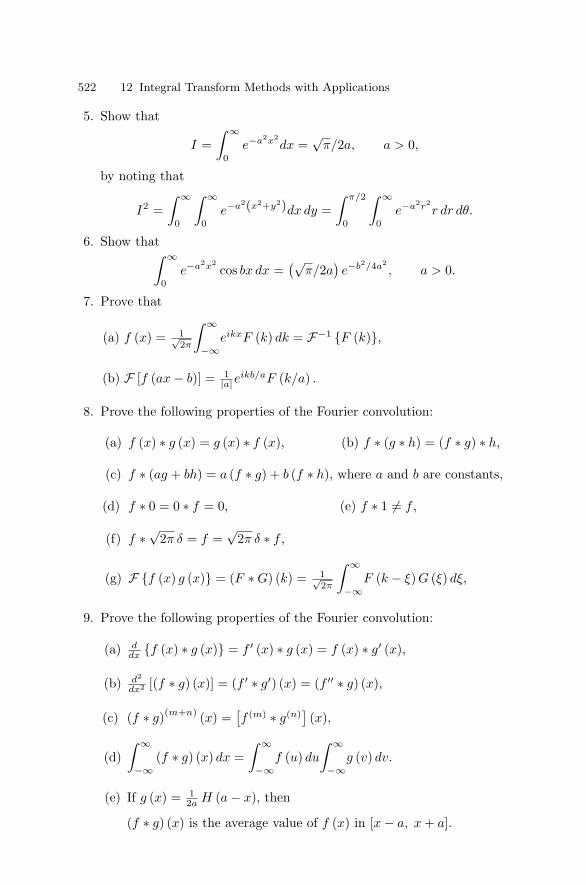
522 12 Integral Transform Methods with Applications
5. Show that
I =∫ ∞
0e−a2x2
dx =√
π/2a, a > 0,
by noting that
I2 =∫ ∞
0
∫ ∞
0e−a2(x2+y2)dx dy =
∫ π/2
0
∫ ∞
0e−a2r2
r dr dθ.
6. Show that∫ ∞
0e−a2x2
cos bx dx =(√
π/2a)e−b2/4a2
, a > 0.
7. Prove that
(a) f (x) = 1√2π
∫ ∞
−∞eikxF (k) dk = F−1 F (k),
(b) F [f (ax − b)] = 1|a|e
ikb/aF (k/a) .
8. Prove the following properties of the Fourier convolution:
(a) f (x) ∗ g (x) = g (x) ∗ f (x), (b) f ∗ (g ∗ h) = (f ∗ g) ∗ h,
(c) f ∗ (ag + bh) = a (f ∗ g) + b (f ∗ h), where a and b are constants,
(d) f ∗ 0 = 0 ∗ f = 0, (e) f ∗ 1 = f ,
(f) f ∗ √2π δ = f =
√2π δ ∗ f ,
(g) F f (x) g (x) = (F ∗ G) (k) = 1√2π
∫ ∞
−∞F (k − ξ) G (ξ) dξ,
9. Prove the following properties of the Fourier convolution:
(a) ddx f (x) ∗ g (x) = f ′ (x) ∗ g (x) = f (x) ∗ g′ (x),
(b) d2
dx2 [(f ∗ g) (x)] = (f ′ ∗ g′) (x) = (f ′′ ∗ g) (x),
(c) (f ∗ g)(m+n) (x) =[f (m) ∗ g(n)
](x),
(d)∫ ∞
−∞(f ∗ g) (x) dx =
∫ ∞
−∞f (u) du
∫ ∞
−∞g (v) dv.
(e) If g (x) = 12a H (a − x), then
(f ∗ g) (x) is the average value of f (x) in [x − a, x + a].

12.18 Exercises 523
(f) If Gt (x) = 1√4πkt
exp(− x2
4κt
), then (Gt ∗ Gs) (x) = Gt+s (x).
10. Prove the following results:
(a) 1√2π
∫ ∞
−∞e−k2t−ikx dk = 1√
2te−x2/4t,
(b)∫ ∞
−∞F (k) g (k) eikx dk =
∫ ∞
−∞f (y) G (y − x) dy,
(c)∫ ∞
−∞F (k) g (k) dk =
∫ ∞
−∞f (y) G (y) dy,
(d) sinx ∗ e−a|x| =√
2π
a sin x(1+a2) , (e) eax ∗ χ[0,∞) (x) = 1
aeax√2π
, a > 0 ,
(f) 1√2a
exp(−x2
4a
)∗ 1√
2bexp
(−x2
4b
)= 1√
2(a+b)exp
(− x2
4(a+b)
).
11. Determine the solution of the initial-value problem
utt = c2uxx, −∞ < x < ∞, t > 0,
u (x, 0) = f (x) , ut (x, 0) = g (x) , −∞ < x < ∞.
12. Solve
ut = uxx, x > 0, t > 0,
u (x, 0) = f (x) , u (0, t) = 0.
13. Solve
utt = c2uxxxx = 0, −∞ < x < ∞, t > 0,
u (x, 0) = f (x) , ut (x, 0) = 0, −∞ < x < ∞.
14. Solve
utt + c2uxxxx = 0, x > 0, t > 0,
u (x, 0) = 0, ut (x, 0) = 0, x > 0,
u (0, t) = g (t) , uxx (0, t) = 0, t > 0.
15. Solve
φxx + φyy = 0, −a < x < a, 0 < y < ∞,
φy (x, 0) =
⎧⎨⎩δ0, 0 < |x| < a,
0, |x| > a.
φ (x, y) → 0 uniformly in x as y → ∞.
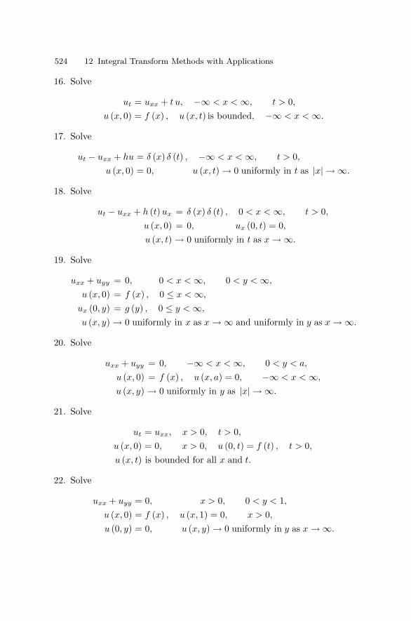
524 12 Integral Transform Methods with Applications
16. Solve
ut = uxx + t u, −∞ < x < ∞, t > 0,
u (x, 0) = f (x) , u (x, t) is bounded, −∞ < x < ∞.
17. Solve
ut − uxx + hu = δ (x) δ (t) , −∞ < x < ∞, t > 0,
u (x, 0) = 0, u (x, t) → 0 uniformly in t as |x| → ∞.
18. Solve
ut − uxx + h (t) ux = δ (x) δ (t) , 0 < x < ∞, t > 0,
u (x, 0) = 0, ux (0, t) = 0,u (x, t) → 0 uniformly in t as x → ∞.
19. Solve
uxx + uyy = 0, 0 < x < ∞, 0 < y < ∞,
u (x, 0) = f (x) , 0 ≤ x < ∞,
ux (0, y) = g (y) , 0 ≤ y < ∞,
u (x, y) → 0 uniformly in x as x → ∞ and uniformly in y as x → ∞.
20. Solve
uxx + uyy = 0, −∞ < x < ∞, 0 < y < a,
u (x, 0) = f (x) , u (x, a) = 0, −∞ < x < ∞,
u (x, y) → 0 uniformly in y as |x| → ∞.
21. Solve
ut = uxx, x > 0, t > 0,
u (x, 0) = 0, x > 0, u (0, t) = f (t) , t > 0,
u (x, t) is bounded for all x and t.
22. Solve
uxx + uyy = 0, x > 0, 0 < y < 1,
u (x, 0) = f (x) , u (x, 1) = 0, x > 0,
u (0, y) = 0, u (x, y) → 0 uniformly in y as x → ∞.

12.18 Exercises 525
23. Find the Laplace transform of each of the following functions:
(a) tn, (b) cos ωt, (c) sinh kt,
(d) cosh kt, (e) teat, (f) eat sin ωt,
(g) eat cos ωt, (h) t sinh kt, (i) t cosh kt,
(j)√
1t , (k)
√t, (l) sin at
t .
24. Find the inverse transform of each of the following functions:
(a) s(s2+a2)(s2+b2) , (b) 1
(s2+a2)(s2+b2) ,
(c) 1(s−a)(s−b) , (d) 1
s(s+a)2 ,
(e) 1s(s+a) , (f) s2−a2
(s2+a2)2 .
25. The velocity potential φ (x, z, t) and the free-surface evaluation η (x, t)for surface waves in water of infinite depth satisfy the Laplace equation
φxx + φzz = 0, −∞ < x < ∞, −∞ < z ≤ 0, t > 0,
with the free-surface, boundary, and initial conditions
φz = ηt on z = 0, t > 0,
φt + gη = 0 on z = 0, t > 0,
φz → 0 as z → −∞,
φ (x, 0, 0) = 0 and η (x, 0) = f (x) , −∞ < x < ∞,
where g is the constant acceleration due to gravity.Show that
φ (x, z, t) = −√
g√2π
∫ ∞
−∞k− 1
2 F (k) e|k|z−ikx sin(√
g |k| t)
dk,
η (x, t) =1√2π
∫ ∞
−∞F (k) e−ikx cos
(√g |k| t
)dk,
where k represents the Fourier transform variable.Find the asymptotic solution for η (x, t) as t → ∞.
26. Use the Fourier transform method to show that the solution of theone-dimensional Schrodinger equation for a free particle of mass m,
iψt = − 2
2mψxx, −∞ < x < ∞, t > 0,
ψ (x, 0) = f (x) , −∞ < x < ∞,

526 12 Integral Transform Methods with Applications
where ψ and ψx tend to zero as |x| → ∞, and h = 2π is the Planckconstant, is given by
ψ (x, t) =1√2π
∫ ∞
−∞f (ξ) G (x − ξ) dξ,
where G (x, t) = (1−i)2√
γtexp
[− x2
4iγt
]is the Green’s function and γ =
2m .
27. Prove the following properties of the Laplace convolution:
(a) f ∗ g = g ∗ f , (b) f ∗ (g ∗ h) = (f ∗ g) ∗ h,
(c) f ∗ (αg + βh) = α (f ∗ g) + β (f ∗ h), α and β are constants,
(d) f ∗ 0 = 0 ∗ f ,
(e) ddt [(f ∗ g) (t)] = f ′ (t) ∗ g (t) + f (0) g (t),
(f) d2
dt2 [(f ∗ g) (t)] = f ′′ (t) ∗ g (t) + f ′ (0) g (t) + f (0) g′ (t),
(g) dn
dtn [(f ∗ g) (t)] = f (n) (t) ∗ g (t) +n−1∑k=0
f (k) (0) g(n−k−1) (t).
28. Obtain the solution of the problem
utt = c2uxx, 0 < x < ∞, t > 0,
u (x, 0) = f (x) , ut (x, 0) = 0,
u (0, t) = 0, u (x, t) → 0 uniformly in t as x → ∞.
29. Solve
utt = c2uxx, 0 < x < l, t > 0,
u (x, 0) = 0, ut (x, 0) = 0,
u (0, t) = f (t) , u (l, t) = 0, t ≥ 0.
30. Solve
ut = κuxx, 0 < x < ∞, t > 0,
u (x, 0) = f0, 0 < x < ∞,
u (0, t) = f1, u (x, t) → f0 uniformly in t as x → ∞, t > 0.
31. Solve
ut = κuxx, 0 < x < ∞, t > 0,
u (x, 0) = x, x > 0,
u (0, t) = 0, u (x, t) → x uniformly in t as x → ∞, t > 0.

12.18 Exercises 527
32. Solve
ut = κuxx, 0 < x < ∞, t > 0,
u (x, 0) = 0, 0 < x < ∞,
u (0, t) = t2, u (x, t) → 0 uniformly in t as x → ∞, t ≥ 0.
33. Solve
ut = κuxx − hu, 0 < x < ∞, t > 0, h = constant,u (x, 0) = f0, x > 0,
u (0, t) = 0, ux (0, t) → 0 uniformly in t as x → ∞, t > 0.
34. Solve
ut = κuxx, 0 < x < ∞, t > 0,
u (x, 0) = 0, 0 < x < ∞,
u (0, t) = f0, u (x, t) → 0 uniformly in t as x → ∞, t > 0.
35. Solve
utt = c2uxx, 0 < x < ∞, t > 0,
u (x, 0) = 0, ut (x, 0) = f0, 0 < x < ∞,
u (0, t) = 0, ux (x, t) → 0 uniformly in t as x → ∞, t > 0.
36. Solve
utt = c2uxx, 0 < x < ∞, t > 0,
u (x, 0) = f (x) , ut (x, 0) = 0, 0 < x < ∞,
u (0, t) = 0, ux (x, t) → 0 uniformly in t as x → ∞, t > 0.
37. A semi-infinite lossless transmission line has no initial current or poten-tial. A time dependent EMF , V0 (t) H (t) is applied at the end x = 0.Find the potential V (x, t). Then determine the potential for cases: (i)V0 (t) = V0 = constant, and (ii) V0 (t) = V0 cos ωt.
38. Solve the Blasius problem of an unsteady boundary layer flow in a semi-infinite body of viscous fluid enclosed by an infinite horizontal disk atz = 0. The governing equation, boundary, and initial conditions are
∂u
∂t= ν
∂2u
∂z2 , z > 0, t > 0,
u (z, t) = Ut on z = 0, t > 0,
u (z, t) → 0 as z → ∞, t > 0,
u (z, t) = 0 at t ≤ 0, z > 0.
Explain the implication of the solution.

528 12 Integral Transform Methods with Applications
39. The stress-strain relation and equation of motion for a viscoelastic rodin the absence of external force are
∂e
∂t=
1E
∂σ
∂t+
σ
η,
∂σ
∂x= ρ
∂2u
∂t2,
where e is the strain, η is the coefficient of viscosity, and the displace-ment u (x, t) is related to the strain by e = ∂u/∂x. Prove that the stressσ (x, t) satisfies the modified wave equation
∂2σ
∂x2 − ρ
η
∂σ
∂t=
1c2
∂2σ
∂t2, c2 = E/ρ.
Show that the stress distribution in a semi-infinite viscoelastic rod sub-ject to the boundary and initial conditions,
u (0, t) = U H (t) , σ (x, t) → 0 as x → ∞, t > 0,
σ (x, 0) = 0, u (x, 0) = 0,
is given by
σ (x, t) = −Uρc exp(
−Et
2η
)I0
[Et
2η
(t2 − x2
c2
) 12]
H(t − x
c
).
40. An elastic string is stretched between x = 0 and x = l and is initiallyat rest in the equilibrium position. Show that the Laplace transformsolution for the displacement field subject to the boundary conditionsy (0, t) = f (t) and y (l, t) = 0, t > 0 is
y (x, s) = f (s)sinh
sc (l − x)
sinh sl
c
.
41. The end x = 0 of a semi-infinite submarine cable is maintained ata potential V0H (t). If the cable has no initial current and potential,determine the potential V (x, t) at point x and at time t.
42. Obtain the solution of the Stokes–Ekman problem (see Debnath, 1995)of an unsteady boundary layer flow in a semi-infinite body of viscousfluid bounded by an infinite horizontal disk at z = 0, when both thefluid and the disk rotate with a uniform angular velocity Ω about the z-axis. The governing boundary layer equation, the boundary conditions,and the initial conditions are
∂q
∂t+ 2Ωiq = ν
∂2q
∂z2 , z > 0, t > 0,
q (z, t) = aeiωt + be−iωt on z = 0, t > 0,
q (z, t) → 0 as z → ∞, t > 0,
q (z, t) = 0 at t ≤ 0, for all z > 0,

12.18 Exercises 529
where q = u + iv, is the complex velocity field, ω is the frequencyof oscillations of the disk, and a and b are complex constants. Hence,deduce the steady-state solution, and determine the structure of theassociated boundary layers.
43. Show that, when ω = 0 in the Stokes–Ekman problem 42, the steadyflow field is given by
q (z, t) ∼ (a + b) exp
−
(2iΩ
ν
) 12
z
.
Hence determine the thickness of the Ekman layer.
44. For problem 14 (e) (iii) in 3.9 Exercises, show that the potential V (x, t)and the current I (x, t) satisfy the partial differential equation(
∂2
∂t2+ 2k
∂
∂t+ k2
)(V, I) = c2 ∂2
∂x2 (V, I) .
Find the solution for V (x, t) with the boundary and initial data
V (x, t) = V0 (t) at x = 0, t > 0,
V (x, t) → 0 as x → ∞, t > 0,
V (x, 0) = Vt (x, 0) = 0 for 0 ≤ x < ∞.
45. Use the Laplace transform to solve the Abel integral equation
g (t) =∫ t
0f ′ (τ) (t − τ)−α
dτ, 0 < α < 1.
46. Solve Abel’s problem of tautochronous motion described in problem 17of 14.11 Exercises.
47. The velocity potential φ (r, z, t) and the free-surface elevation η (r, t)for axisymmetric surface waves in water of infinite depth satisfy theequation
φrr +1rφr + φzz = 0, 0 ≤ r < ∞, −∞ < z ≤ 0, t > 0,
with the free-surface, boundary, and initial conditions
φz = ηz on z = 0, t > 0,
φt + gη = 0, on z = 0, t > 0,
φz → 0, z → −∞,
φ (r, 0, 0) = 0, and η (r, 0) = f (r) , 0 ≤ r < ∞,
where g is the acceleration due to gravity and f (r) represents the initialelevation.Show that

530 12 Integral Transform Methods with Applications
φ (r, z, t) = −√g
∫ ∞
0
√k f (k) J0 (kr) ekz sin
(√gk t
)dk,
η (r, t) =∫ ∞
0k f (k) J0 (kr) cos
(√gk t
)dk,
where f (k) is the zero-order Hankel transform of f (r).Derive the asymptotic solution
η (r, t) ∼ gt2
232 r3
f
(gt2
4r2
)cos
(gt2
4r
)as t → ∞.
48. Write the solution for the Cauchy–Poisson problem where the initialelevation is concentrated in the neighborhood of the origin, that is,f (r) = (a/2πr) δ (r), where a is the total volume of the fluid displaced.
49. The steady temperature distribution u (r, z) in a semi-infinite solid withz ≥ 0 is governed by the system
urr +1rur + uzz = −Aq (r) , 0 < r < ∞, z > 0,
u (r, 0) = 0,
where A is a constant and q (r) represents the steady heat source. Showthat the solution is given by
u (r, z) = A
∫ ∞
0q (k) J0 (kr) k−1 (
1 − e−kz)dk,
where q (k) is the zero-order Hankel transform of q (r).
50. Find the solution for the small deflection u (r) of an elastic membranesubjected to a concentrated loading distribution which is governed by
urr +1rur − κ2u =
12π
δ (r)r
, 0 ≤ r < ∞,
where u and its derivatives vanish as r → ∞.
51. Obtain the solution for the potential v (r, z) due to a flat electrified diskof radius unity with the center of the disk at the origin and the axisalong the z-axis. The function v (r, z) satisfies the Laplace equation
vrr +1rvr − vzz = 0, 0 < r < ∞, z > 0,
with the boundary conditions
v (r, 0) = v0, 0 ≤ r < 1,
vz (r, 0) = 0, r > 1.
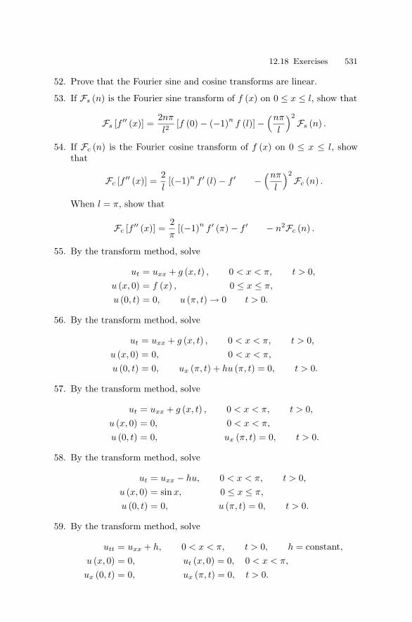
12.18 Exercises 531
52. Prove that the Fourier sine and cosine transforms are linear.
53. If Fs (n) is the Fourier sine transform of f (x) on 0 ≤ x ≤ l, show that
Fs [f ′′ (x)] =2nπ
l2[f (0) − (−1)n
f (l)] −(nπ
l
)2Fs (n) .
54. If Fc (n) is the Fourier cosine transform of f (x) on 0 ≤ x ≤ l, showthat
Fc [f ′′ (x)] =2l
[(−1)nf ′ (l) − f ′ (0)] −
(nπ
l
)2Fc (n) .
When l = π, show that
Fc [f ′′ (x)] =2π
[(−1)nf ′ (π) − f ′ (0)] − n2Fc (n) .
55. By the transform method, solve
ut = uxx + g (x, t) , 0 < x < π, t > 0,
u (x, 0) = f (x) , 0 ≤ x ≤ π,
u (0, t) = 0, u (π, t) → 0 t > 0.
56. By the transform method, solve
ut = uxx + g (x, t) , 0 < x < π, t > 0,
u (x, 0) = 0, 0 < x < π,
u (0, t) = 0, ux (π, t) + hu (π, t) = 0, t > 0.
57. By the transform method, solve
ut = uxx + g (x, t) , 0 < x < π, t > 0,
u (x, 0) = 0, 0 < x < π,
u (0, t) = 0, ux (π, t) = 0, t > 0.
58. By the transform method, solve
ut = uxx − hu, 0 < x < π, t > 0,
u (x, 0) = sinx, 0 ≤ x ≤ π,
u (0, t) = 0, u (π, t) = 0, t > 0.
59. By the transform method, solve
utt = uxx + h, 0 < x < π, t > 0, h = constant,u (x, 0) = 0, ut (x, 0) = 0, 0 < x < π,
ux (0, t) = 0, ux (π, t) = 0, t > 0.

532 12 Integral Transform Methods with Applications
60. By the transform method, solve
utt = uxx + g (x) , 0 < x < π, t > 0,
u (x, 0) = 0, ut (x, 0) = 0, 0 < x < π,
u (0, t) = 0, u (π, t) = 0, t > 0.
61. By the transform method, solve
utt + c2uxxxx = 0, 0 < x < π, t > 0,
u (x, 0) = 0, ut (x, 0) = 0, 0 < x < π,
u (0, t) = 0, u (π, t) = 0, t > 0.
uxx (0, t) = 0, uxx (π, t) = sin t, t ≥ 0.
62. Find the temperature distribution u (r, t) in a long cylinder of radiusa when the initial temperature is constant, u0, and radiation occurs atthe surface into a medium with zero temperature. Here u (r, t) satisfiesthe initial boundary-problem
ut = κ
(urr +
1rur
), 0 ≤ r < a, t > 0,
ur + α u = 0 at r = a, t > 0,
u (r, 0) = u0 for 0 ≤ r < a,
where κ and α are constants.
63. Apply the finite Fourier sine transform to solve the longitudinal dis-placement field in a uniform bar of length l and cross section A sub-jected to an external force FA applied at the end x = l. The governingequation and boundary and initial conditions are
c2uxx = utt,
(c2 =
E
ρ
), 0 < x < l, t > 0,
u (0, t) = 0 E u (l, t) = F, t > 0,
u (x, 0) = ut (x, 0) = 0, 0 < x < l,
where E is the constant Young’s modulus, ρ is the density, and F isconstant.
64. Use the finite Fourier cosine transform to solve the heat conductionproblem
ut = κuxx, 0 < x < l, t > 0,
ux (x, t) = 0 at x = 0 and x = l, t > 0,
u (x, 0) = u0 for 0 < x < l,
where u0 and κ are constant.

12.18 Exercises 533
65. Use the Mellin transform to find the solution of the integral equation∫ ∞
−∞f (x) k (xt) dx = g (t) , t > 0.
66. Use the Mellin transform to show the following results:
(a)∞∑
n=1
f (n) = 12πi
∫ c+i∞
c−i∞ζ (p) F (p) dp,
(b)∞∑
n=1
f (nx) = M−1 [ζ (p) F (p)],
where ζ (s) is the Riemann zeta function defined by (6.7.13).
67. Show that the solution of the boundary-value problem
urr +1rur + uzz = 0, r ≥ 0, z > 0,
u (r, 0) = u0 for 0 ≤ r ≤ a,
u (r, z) → 0 as z → ∞,
is
u (r, z) = au0
∫ ∞
0J1 (ak) J0 (kr) e−kzdk.
68. Show that the asymptotic representation of the Bessel function Jn (kr)for large kr is
Jn (kr) =1π
∫ π
0cos (nθ − kr sin θ) dθ ∼
(2
πkr
) 12
cos(kr − nπ
2− π
4
).
69. (a) Use the Laplace transform to solve the heat conduction problem
ut = κuxx, 0 < x < ∞, t > 0,
u (x, 0) = 0, x > 0,
u (0, t) = f (t) , u (x, t) → 0 as x → ∞, t > 0.
(b) Derive Duhamel’s formula
u (x, t) =∫ t
0f (t − τ)
(∂u0
∂τ
)dτ,
where (∂u0
∂t
)=
x√4πκ
t−3/2 exp(
− x2
4κt
).

13
Nonlinear Partial Differential Equations withApplications
“True Laws of Nature cannot be linear.”
Albert Einstein
“... the progress of physics will to a large extent depend on the progressof nonlinear mathematics, of methods to solve nonlinear equations ... andtherefore we can learn by comparing different nonlinear problems.”
Werner Heisenberg
13.1 Introduction
The three-dimensional linear wave equation
utt = c2 ∇2u, (13.1.1)
arises in the areas of elasticity, fluid dynamics, acoustics, magnetohydrody-namics, and electromagnetism.
The general solution of the one-dimensional equation (13.1.1) is
u (x, t) = φ (x − ct) + ψ (x + ct) , (13.1.2)
where φ and ψ are determined by the initial or boundary conditions. Phys-ically, φ and ψ represent waves moving with constant speed c and withoutchange of shape, along the positive and the negative directions of x respec-tively.
The solutions φ and ψ correspond to the two factors when the one-dimensional equation (13.1.1) is written in the form(
∂
∂t+ c
∂
∂x
)(∂
∂t− c
∂
∂x
)u = 0. (13.1.3)
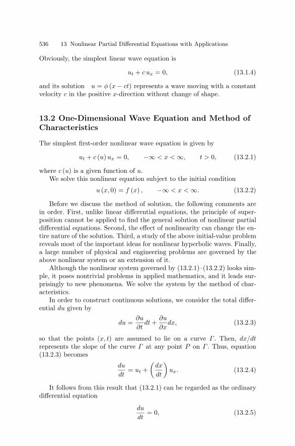
536 13 Nonlinear Partial Differential Equations with Applications
Obviously, the simplest linear wave equation is
ut + c ux = 0, (13.1.4)
and its solution u = φ (x − ct) represents a wave moving with a constantvelocity c in the positive x-direction without change of shape.
13.2 One-Dimensional Wave Equation and Method ofCharacteristics
The simplest first-order nonlinear wave equation is given by
ut + c (u) ux = 0, −∞ < x < ∞, t > 0, (13.2.1)
where c (u) is a given function of u.We solve this nonlinear equation subject to the initial condition
u (x, 0) = f (x) , −∞ < x < ∞. (13.2.2)
Before we discuss the method of solution, the following comments arein order. First, unlike linear differential equations, the principle of super-position cannot be applied to find the general solution of nonlinear partialdifferential equations. Second, the effect of nonlinearity can change the en-tire nature of the solution. Third, a study of the above initial-value problemreveals most of the important ideas for nonlinear hyperbolic waves. Finally,a large number of physical and engineering problems are governed by theabove nonlinear system or an extension of it.
Although the nonlinear system governed by (13.2.1)–(13.2.2) looks sim-ple, it poses nontrivial problems in applied mathematics, and it leads sur-prisingly to new phenomena. We solve the system by the method of char-acteristics.
In order to construct continuous solutions, we consider the total differ-ential du given by
du =∂u
∂tdt +
∂u
∂xdx, (13.2.3)
so that the points (x, t) are assumed to lie on a curve Γ . Then, dx/dtrepresents the slope of the curve Γ at any point P on Γ . Thus, equation(13.2.3) becomes
du
dt= ut +
(dx
dt
)ux. (13.2.4)
It follows from this result that (13.2.1) can be regarded as the ordinarydifferential equation
du
dt= 0, (13.2.5)

13.2 One-Dimensional Wave Equation and Method of Characteristics 537
along any member of the family of curves Γ which are the solution curvesof
dx
dt= c (u) . (13.2.6)
These curves Γ are called the characteristic curves of the main equation(13.2.1). Thus, the solution of (13.2.1) has been reduced to the solution ofa pair of simultaneous ordinary differential equations (13.2.5) and (13.2.6).Clearly, both the characteristic speed and the characteristics depend on thesolution u.
Equation (13.2.5) implies that u = constant along each characteristiccurve Γ , and each c (u) remains constant on Γ . Therefore, (13.2.6) showsthat the characteristic curves of (13.2.1) form a family of straight lines inthe (x, t)-plane with slope c (u). This indicates that the general solution of(13.2.1) depends on finding the family of lines. Also, each line with slopec (u) corresponds to the value of u on it. If the initial point on the charac-teristic curve Γ is denoted by ξ and if one of the curves Γ intersects t = 0at x = ξ, then u (ξ, 0) = f (ξ) on the whole of that curve Γ as shown inFigure 13.2.1.
Thus, we have the following characteristic form on Γ :
dx
dt= c (u) , x (0) = ξ, (13.2.7)
du
dt= 0, u (ξ, 0) = f (ξ) . (13.2.8)
These constitute a pair of coupled ordinary differential equations on Γ .Equation (13.2.7) cannot be solved independently because c is a function
of u. However, (13.2.8) can readily be solved to obtain u = constant and
Figure 13.2.1 A characteristic curve.

538 13 Nonlinear Partial Differential Equations with Applications
hence, u = f (ξ) on the whole of Γ . Thus, (13.2.7) leads to
dx
dt= F (ξ) , x (0) = ξ, (13.2.9)
where
F (ξ) = c (f (ξ)) . (13.2.10)
Integrating equation (13.2.9) gives
x = tF (ξ) + ξ. (13.2.11)
This represents the characteristic curve which is a straight line whose slopeis not a constant, but depends on ξ.
Combining these results, we obtain the solution of the initial-value prob-lem in parametric form
u (x, t)x
==
f (ξ)ξ + t F (ξ)
, (13.2.12)
where
F (ξ) = c (f (ξ)) .
We next verify that this final form represents an analytic expression ofthe solution. Differentiating (13.2.12) with respect to x and t, we obtain
ux = f ′ (ξ) ξx, ut = f ′ (ξ) ξt,
1 = 1 + tF ′ (ξ) ξx,
0 = F (ξ) + 1 + tF ′ (ξ) ξt.
Elimination of ξx and ξt gives
ux =f ′ (ξ)
1 + tF ′ (ξ), ut = −F (ξ) f ′ (ξ)
1 + tF ′ (ξ). (13.2.13)
Since F (ξ) = c (f (ξ)), equation (13.2.1) is satisfied provided 1+tF ′ (ξ) = 0.The solution (13.2.12) also satisfies the initial condition at t = 0, since
ξ = x, and the solution (13.2.12) is unique.Suppose that u (x, t) and v (x, t) are two solutions. Then, on x = ξ +
tF (ξ),
u (x, t) = u (ξ, 0) = f (ξ) = v (x, t) .
Thus, we have proved the following:

13.2 One-Dimensional Wave Equation and Method of Characteristics 539
Theorem 13.2.1. The nonlinear initial-value problem
ut + c (u) ux = 0, −∞ < x < ∞, t > 0,
u (x, t) = f (x) , at t = 0, −∞ < x < ∞,
has a unique solution provided 1+tF ′ (ξ) = 0, f and c are C1 (R) functionswhere F (ξ) = c (f (ξ)).
The solution is given in the parametric form:
u (x, t) = f (ξ) ,
x = ξ + tF (ξ) .
Remark: When c (u) = constant = c > 0, equation (13.2.1) becomes thelinear wave equation (13.1.4). The characteristic curves are x = ct + ξ andthe solution u is given by
u (x, t) = f (ξ) = f (x − ct) .
Physical Significance of (13.2.12).
We assume c (u) > 0. The graph of u at t = 0 is the graph of f . In view ofthe fact
u (x, t) = u (ξ + tF (ξ) , t) = f (ξ)
the point (ξ, f (ξ)) moves parallel to the x-axis in the positive directionthrough a distance tF (ξ) = ct, and the distance moved (x = ξ + ct) de-pends on ξ. This is a typical nonlinear phenomenon. In the linear case, thecurve moves parallel to the x-axis with constant velocity c, and the solu-tion represents waves travelling without change of shape. Thus, there is astriking difference between the linear and the nonlinear solution.
Theorem 13.2.1 asserts that the solution of the nonlinear initial-valueproblem exists provided
1 + tF ′ (ξ) = 0, x = ξ + tF ′ (ξ) . (13.2.14)
However, the former condition is always satisfied for sufficiently small timet. By a solution of the problem, we mean a differentiable function u (x, t).It follows from results (13.2.13) that both ux and ut tend to infinity as1 + tF ′ (ξ) → 0. This means that the solution develops a singularity (dis-continuity) when 1+ tF ′ (ξ) = 0. We consider a point (x, t) = (ξ, 0) so thatthis condition is satisfied on the characteristics through the point (ξ, 0) ata time t such that
t = − 1F ′ (ξ)
(13.2.15)

540 13 Nonlinear Partial Differential Equations with Applications
which is positive provided F ′ (ξ) = c′ (f) f ′ (ξ) < 0. If we assume c′ (f) > 0,the above inequality implies that f ′ (ξ) < 0. Hence, the solution (13.2.12)ceases to exist for all time if the initial data is such that f ′ (ξ) < 0 for somevalue of ξ. Suppose t = τ is the time when the solution first develops asingularity (discontinuity) for some value of ξ. Then
τ = − 1min−∞<ξ<∞ c′ (f) f ′ (ξ) > 0.
We draw the graphs of the nonlinear solution u (x, t) = f (ξ) below fordifferent values of t = 0, τ , 2τ , . . .. The shape of the initial curve for u (x, t)changes with increasing values of t, and the solution becomes multiple-valued for t ≥ τ . Therefore, the solution breaks down when F ′ (ξ) < 0 forsome ξ, and such breaking is a typical nonlinear phenomenon. In lineartheory, such breaking will never occur.
More precisely, the development of a singularity in the solution for t ≥ τcan be seen by the following consideration. If f ′ (ξ) < 0, we can find twovalues of ξ = ξ1, ξ2 (ξ1 < ξ2) on the initial line such that the characteristicsthrough them have different slopes 1/c (u1) and 1/c (u2) where u1 = f (ξ1)and u2 = f (ξ2) and c (u2) < c (u1). Thus, these two characteristics willintersect at a point in the (x, t)-plane for some t > 0. Since the character-istics carry constant values of u, the solution ceases to be single-valued attheir point of intersection. Figure 13.2.2 shows that the wave profile pro-gressively distorts itself, and at any instant of time there exists an intervalon the x-axis, where u assumes three values for a given x. The end resultis the development of a nonunique solution, and this leads to breaking.
Therefore, when conditions (13.2.14) are violated the solution developsa discontinuity known as a shock. The analysis of shock involves extensionof a solution to allow for discontinuities. Also, it is necessary to impose onthe solution certain restrictions to be satisfied across its discontinuity. Thispoint will be discussed further in a subsequent section.
13.3 Linear Dispersive Waves
We consider a single linear partial differential equation with constant coef-ficients in the form
P
(∂
∂t,
∂
∂x,
∂
∂y,
∂
∂z
)u (x, t) = 0, (13.3.1)
where P is a polynomial in partial derivatives and x = (x, y, z).We seek an elementary plane wave solution of (13.3.1) in the form
u (x, t) = a ei(κκκ·x−ωt), (13.3.2)
where a is the amplitude, κκκ = (k, l, m) is the wavenumber vector, ω isthe frequency and a, κκκ, ω are constants. When this plane wave solution is

13.3 Linear Dispersive Waves 541
Figure 13.2.2 The solution u (x, t) for different times t = 0, τ and 2τ ; thecharacteristics are shown by the dotted lines; two of them from x = ξ1 andx = ξ2 intersect at t > τ .
substituted in the equation, ∂/∂t, ∂/∂x, ∂/∂y, and ∂/∂z produce factors−iω, ik, il, and im respectively, and the solution exists provided ω and κκκare related by an equation
P (−iω, ik, il, im) = 0. (13.3.3)
This equation is known as the dispersion relation. Evidently, we have adirect correspondence between equation (13.3.1) and the dispersion relation(13.3.3) through the correspondence
∂
∂t↔ −iω,
(∂
∂x,
∂
∂y,
∂
∂z
)↔ i (k, l, m) . (13.3.4)
Equation (13.3.1) and the corresponding dispersion relation (13.3.3) in-dicate that the former can be derived from the latter and vice-versa by us-ing (13.3.4). The dispersion relation characterizes the plane wave motion.In many problems, the dispersion relation can be written in the explicitform
ω = W (k, l, m) . (13.3.5)
The phase and the group velocities of the waves are defined by
Cp (κκκ) =ω
κκκκ, (13.3.6)
Cg (κκκ) = ∇κκκω, (13.3.7)

542 13 Nonlinear Partial Differential Equations with Applications
where κκκ is the unit vector in the direction of wave vector κκκ.In the one-dimensional case, (13.3.5)–(13.3.7) become
ω = W (k) , Cp =ω
k, Cg =
dω
dk. (13.3.8)
The one-dimensional waves given by (13.3.2) are called dispersive if thegroup velocity Cg ≡ ω′ (k) is not constant, that is, ω′′ (k) = 0. Physically,as time progresses, the different waves disperse in the medium with theresult that a single hump breaks into wavetrains.
Example 13.3.1.
(i) Linearized one-dimensional wave equation
utt − c2uxx = 0, ω = + ck. (13.3.9)
(ii) Linearized Korteweg and de Vries (KdV) equation for long water waves
ut + αux + βuxxx = 0, ω = αk − βk3. (13.3.10)
(iii) Klein–Gordon equation
utt − c2uxx + α2u = 0, ω = +(c2k2 + α2) 1
2 . (13.3.11)
(iv) Schrodinger equation in quantum mechanics and de Broglie waves
i ψt −(
V − 2
2m∇2
)ψ = 0, ω =
2κ2
2m+ V, (13.3.12)
where V is a constant potential energy, and h = 2π is the Planckconstant.
The group velocity of de Broglie wave is (κκκ/m), and through the corre-spondence principle, ω is to be interpreted as the total energy,
(
2κκκ2/2m)
as the kinetic energy, and κκκ as the particle momentum. Hence, the groupvelocity is the classical particle velocity.
(v) Equation for vibration of a beam
utt + α2uxxxx = 0, ω = +αk2. (13.3.13)
(vi) The dispersion relation for water waves in an ocean of depth h
ω2 = gk tanh kh, (13.3.14)
where g is the acceleration due to gravity.

13.3 Linear Dispersive Waves 543
(vii) The Boussinesq equation
utt − α2∇2u − β2∇2utt = 0, ω = +ακ√
1 + β2κ2. (13.3.15)
This equation arises in elasticity for longitudinal waves in bars, longwater waves, and plasma waves.
(viii) Electromagnetic waves in dielectrics(utt + ω2
0u) (
utt − c20uxx
) − ω2putt = 0,(
ω2 − ω20) (
ω2 − c20k
2) − ω2pω2 = 0, (13.3.16)
where ω0 is the natural frequency of the oscillator, c0 is the speed oflight, and ωp is the plasma frequency.
In view of the superposition principle, the general solution can be obtainedfrom (13.3.2) with the dispersion solution (13.3.3). For the one-dimensionalcase, the general solution has the Fourier integral representation
u (x, t) =∫ ∞
−∞F (k) ei[kx−tW (k)]dk, (13.3.17)
where F (k) is chosen to satisfy the initial or boundary data provided thedata are physically realistic enough to have Fourier transforms.
In many cases, as cited in Example 13.3.1, there are two modes ω =+ W (k) so that the solution (13.3.17) has the form
u (x, t) =∫ ∞
−∞F1 (k) ei[kx−tW (k)]dk +
∫ ∞
−∞F2 (k) ei[kx−tW (k)]dk, (13.3.18)
with the initial data at t = 0
u (x, t) = φ (x) , ut (x, t) = ψ (x) . (13.3.19)
The initial conditions give
φ (x) =∫ ∞
−∞[F1 (k) + F2 (k)] eikxdk,
ψ (x) = −i
∫ ∞
−∞[F1 (k) + F2 (k)] W (k) eikxdk.
Applying the Fourier inverse transformations, we have
F1 (k) + F2 (k) = Φ (k) =1√2π
∫ ∞
−∞φ (x) e−ikxdx,
−iW (k) [F1 (k) − F2 (k)] = Ψ (k) =1√2π
∫ ∞
−∞ψ (x) e−ikxdx,

544 13 Nonlinear Partial Differential Equations with Applications
so that
[F1 (k) + F2 (k)] =12
[Φ (k) +
i Ψ (k)W (k)
]. (13.3.20)
The asymptotic behavior of u (x, t) for large t with fixed (x/t) can beobtained by the Kelvin stationary phase approximation. For real φ (x),ψ (x), Φ (−k) = Φ∗ (k) and Ψ (−k) = Ψ∗ (k), where the asterisk denotes acomplex conjugate. It follows from (13.3.20) that, for W (k) even
[F1 (−k) , F2 (−k)] = [F ∗2 (k) , F ∗
1 (k)] , (13.3.21)
and for W (k) odd,
[F1 (−k) , F2 (−k)] = [F ∗1 (k) , F ∗
2 (k)] . (13.3.22)
In particular, when φ (x) = δ (x) and ψ (x) ≡ 0, then F1 (k) = F2 (k) =1/
√8π, and the solution (13.3.18) reduces to the form
u (x, t) =
√2π
∫ ∞
0cos kx cos tW (k) dk. (13.3.23)
In order to obtain the asymptotic approximation by the Kelvin station-ary phase method (see Section 12.7) for t → ∞, we consider both caseswhen W (k) is even (W ′ (k) is odd) and when W (k) is odd (W ′ (k) is even)and make an extra reasonable assumption that W ′ (k) is monotonic andpositive for k > 0. It turns out that the asymptotic solution for t → ∞ is
u (x, t) ∼ 2 Re
F1 (k)
2π
t |W ′′ (k)| 1
2
exp[i
θ (x, t) − π
4sgn W ′′ (k)
]
+ O
(1t
),
= Re[a (x, t) eiθ(x,t)
], (13.3.24)
where k (x, t) is the positive root of the equation
W ′ (k) =x
t, ω = W (k) ,
x
t> 0, (13.3.25ab)
θ (x, t) = x k (x, t) − t ω (x, t) , (13.3.26)
and
a (x, t) = 2F1 (k)
2π
t |W ′′ (k)| 1
2
exp
− iπ
4sgn W ′′ (k)
. (13.3.27)
It is important to point out that solution (13.3.24) has a form similarto that of the elementary plane wave solution, but k, ω, and a are no

13.4 Nonlinear Dispersive Waves and Whitham’s Equations 545
longer constants; they are functions of space variable x and time t. Thesolution still represents an oscillatory wavetrain with the phase functionθ (x, t) describing the variations between local maxima and minima. Unlikethe elementary plane wavetrain, the present asymptotic result (13.3.24)represents a nonuniform wavetrain in the sense that the amplitude, thedistance, and the time between successive maxima are not constant.
It also follows from (13.3.25a) that
kt
k= − W ′ (k)
kW ′′ (k) t
1t
∼ O
(1t
), (13.3.28)
kx
k= − 1
kW ′′ (k)1t
∼ O
(1t
). (13.3.29)
These results indicate the k (x, t) is a slowly varying function of x and t ast → ∞. Applying a similar argument to ω and a, we conclude that k (x, t),ω (x, t), and a (x, t) are slowly varying functions of x and t as t → ∞.
Finally, all these results seem to provide an important clue for naturalgeneralization of the concept of nonlinear and nonuniform wavetrains.
13.4 Nonlinear Dispersive Waves and Whitham’sEquations
To describe a slowly varying nonlinear and nonuniform oscillatory wavetrainin a medium (see Whitham, 1974), we assume the existence of a solutionin the form (13.3.24) so that
u (x, t) = a (x, t) eiθ(x,t) + c.c., (13.4.1)
where c.c. stands for the complex conjugate, a (x, t) is the complex ampli-tude given by (13.3.27), and the phase function θ (x, t) is
θ (x, t) = x k (x, t) − t ω (x, t) , (13.4.2)
and k, ω, and a are slowly varying function of x and t.Due to slow variations of k and ω, it is reasonable to assume that these
quantities still satisfy the dispersion relation
ω = W (k) . (13.4.3)
Differentiating (13.4.2) with respect to x and t respectively, we obtain
θx = k + x − t W ′ (k) kx, (13.4.4)θt = −W (k) + x − t W ′ (k) kt. (13.4.5)
In the neighborhood of stationary points defined by (13.3.25a), theseresults become

546 13 Nonlinear Partial Differential Equations with Applications
θx = k (x, t) , θt = −ω (x, t) . (13.4.6)
These results can be used as a definition of local wavenumber and localfrequency of the slowly varying nonlinear wavetrain.
In view of (13.4.6), relation (13.4.3) gives a nonlinear partial differentialequation for the phase θ in the form
∂θ
∂t+ W
(∂θ
∂x
)= 0. (13.4.7)
The solution of this equation determines the geometry of the wave pattern.However, it is convenient to eliminate θ from (13.4.6) to obtain
∂k
∂t+
∂ω
∂t= 0. (13.4.8)
This is known as the Whitham equation for the conservation of waves, wherek represents the density of waves and ω is the flux of waves.
Using the dispersion relation (13.4.3), we obtain
∂k
∂t+ Cg (k)
∂k
∂x= 0, (13.4.9)
where Cg (k) = W ′ (k) is the group velocity. This represents the simplestnonlinear wave (hyperbolic) equation for the propagation of k with thegroup velocity Cg (k).
Since equation (13.4.9) is similar to (13.2.1), we can use the analysis ofSection 13.2 to find the general solution of (13.4.9) with the initial conditionk (x, 0) = f (x) at t = 0. In this case, the solution has the form
k (x, t) = f (ξ) , x = ξ + tF (ξ) , (13.4.10)
where F (ξ) = Cg (f (ξ)). This further confirms the propagation of k withthe velocity Cg. Some physical interpretations of this kind of solution havealready been discussed in Section 13.2.
Equations (13.4.9) and (13.4.3) reveal that ω also satisfies the nonlinearwave (hyperbolic) equation
∂ω
∂t+ W ′ (k)
∂ω
∂x= 0. (13.4.11)
It follows from equations (13.4.9) and (13.4.11) that both k and ω remainconstant on the characteristic curves defined by
dx
dt= W ′ (k) = Cg (k) , (13.4.12)
in the (x, t) plane. Since k and ω is constant on each curve, the characteristiccurves are straight lines with slope Cg (k). The solution for k is given by(13.4.10).

13.4 Nonlinear Dispersive Waves and Whitham’s Equations 547
Finally, it follows from the above analysis that any constant value ofthe phase θ propagates according to θ (x, t) = constant, and hence,
θt +(
dx
dt
)θx = 0, (13.4.13)
which gives, by (13.4.6),
dx
dt= − θt
θx=
ω
k= Cp. (13.4.14)
Thus, the phase of the waves propagates with the phase speed Cp. On theother hand, (13.4.9) ensures that the wavenumber k propagates with thegroup velocity Cg (k) = (dω/dk) = W ′ (k).
We next investigate how the wave energy propagates in the dispersivemedium. We consider the following integral involving the square of the waveamplitude (energy) given by (13.3.24) between any two points x = x1 andx = x2 (0 < x1 < x2)
Q (t) =∫ x2
x1
|a|2 dx =∫ x2
x1
aa∗dx, (13.4.15)
= 8π
∫ x2
x1
F1 (k) F ∗1 (k)
t |W ′′ (k)| dx, (13.4.16)
which is, due to a change of variable x = t W ′ (k),
= 8π
∫ k2
k1
F1 (k) F ∗1 (k) dk, (13.4.17)
where kr = t W ′ (kr), r = 1, 2.When kr is kept fixed as t varies, Q (t) remains constant so that
0 =dQ
dt=
d
dt
∫ x2
x1
|a|2 dx,
=∫ x2
x1
∂
∂t|a|2 dx + |a|22 W ′ (k2) − |a|21 W ′ (k1) . (13.4.18)
In the limit x2 − x1 → 0, this result reduces to the partial differentialequation
∂
∂t|a|2 +
∂
∂x
[W ′ (k) |a|2
]= 0. (13.4.19)
This represents the equation for the conservation of wave energy, where |a|2and |a|2 W ′ (k) are the energy density and energy flux respectively. It alsofollows that the energy propagates with the group velocity W ′ (k). It hasbeen shown that the wavenumber k also propagates with the group velocity.Evidently, the group velocity plays a double role.

548 13 Nonlinear Partial Differential Equations with Applications
The above analysis reveals another important fact; equations (13.4.3),(13.4.8), and (13.4.19) constitute a closed set of equations for the threequantities k, ω, and a. Indeed, these are the fundamental equations fornonlinear dispersive waves and are known as Whitham’s equations.
13.5 Nonlinear Instability
For infinitesimal waves, the wave amplitude (ak 1) is very small, so thatnonlinear effects can be neglected altogether. However, for finite ampli-tude waves the terms involving a2 cannot be neglected, and the effects ofnonlinearity become important. In the theory of water waves, Stokes firstobtained the connection due to inherent nonlinearity between the wave-profile and the frequency of a steady periodic wave system. According tothe Stokes theory, the remarkable fact is the dependence of ω on a whichcouples (13.4.8) to (13.4.19). This leads to a new nonlinear phenomenon.
For finite amplitude waves, the frequency ω has the Stokes expansion
ω = ω0 (k) + a2ω2 (k) + . . . = ω(k, a2) . (13.5.1)
This can be regarded as the nonlinear dispersion relation which depends onboth k and a2. In the linear case, the amplitude a → 0, (13.5.1) gives thelinear dispersion relation (13.4.3), that is, ω = ω0 (k).
In order to discuss nonlinear instability, we substitute (13.5.1) into(13.4.8) and retain (13.4.19) in the linear approximation to obtain the fol-lowing coupled system:
∂k
∂t+
∂
∂x+
ω0 (k) + ω2 (k) a2 = 0, (13.5.2)
∂a2
∂t+
∂
∂x
ω′
0 (k) a2 = 0, (13.5.3)
where W (k) ≡ ω0 (k).These equations can be further approximated to obtain
∂k
∂t+ ω′
0∂k
∂x+ ω2
∂a2
∂x= O
(a2) , (13.5.4)
∂a2
∂t+ ω′
0∂a2
∂x+ ω′′
0a2 ∂k
∂x= 0. (13.5.5)
In matrix form, these equations read⎛⎝ ω′0 ω2
ω′′0a2 ω′
0
⎞⎠⎛⎝ ∂k∂x
∂a2
∂x
⎞⎠ +
⎛⎝ 1 0
0 1
⎞⎠⎛⎝ ∂k∂t
∂a2
∂t
⎞⎠ = 0. (13.5.6)
Hence, the eigenvalues λ are the roots of the determinant equation

13.6 The Traffic Flow Model 549
|aij − λ bij | =
∣∣∣∣∣∣ω′
0 − λ ω2
ω′′0a2 ω′
0 − λ
∣∣∣∣∣∣ = 0, (13.5.7)
where aij and bij are the coefficient matrices of (13.5.6). This equation givesthe characteristic velocities
λ =dx
dt= ω′
0 + (ω2ω′′0 )
12 a + O
(a2) . (13.5.8)
If ω2ω′′0 > 0, the characteristics are real and the system is hyperbolic.
The double characteristic velocity splits into two separate real velocities.This provides a new extension of the group velocity to nonlinear problems. Ifthe disturbance is initially finite in extent, it would eventually split into twodisturbances. In general, any initial disturbance or modulating source wouldintroduce disturbances in both families of characteristics. In the hyperboliccase, compressive modulation will progressively distort and steepen so thatthe question of breaking will arise. These results are remarkably differentfrom those found in linear theory, where there is only one characteristicvelocity and any hump may distort, due to the dependence of ω′
0 (k) on k,but would never split.
On the other hand, if ω2ω′′0 < 0, the characteristics are complex and the
system is elliptic. This leads to ill-posed problems. Any small perturbationsin k and a will be given by the solutions of the form exp [iα (x − λt)] where λis calculated from (13.5.8) for unperturbed values of k and a. In this ellipticcase, λ is complex, and the perturbation will grow as t → ∞. Hence, theoriginal wavetrain will become unstable. In the linear theory, the ellipticcase does not arise at all.
Example 13.5.1. For Stokes waves in deep water, the dispersion relation is
ω = (gk)12
(1 +
12k2a2
), (13.5.9)
so that ω0 (k) = (gk)12 and ω2 (k) = 1
2√
g k32 .
In this case, ω′′0 (k) = − 1
4√
g k− 32 so that ω′′
0ω2 = − g8k < 0. The con-
clusion is that Stokes waves in deep water are definitely unstable. This isone of the most remarkable results in the theory of nonlinear water wavesdiscovered during the 1960’s.
13.6 The Traffic Flow Model
We consider the flow of cars on a long highway under the assumptions thatcars do not enter or leave the highway at any one of its points. We take thex-axis along the highway and assume that the traffic flows in the positive

550 13 Nonlinear Partial Differential Equations with Applications
direction. Suppose ρ (x, t) is the density representing the number of carsper unit length at the point x of the highway at time t, and q (x, t) is theflow of cars per unit time.
We assume a conservation law which states that the change in the totalamount of a physical quantity contained in any region of space must beequal to the flux of that quantity across the boundary of that region. Inthis case, the time rate of change of the total number of cars in any segmentx1 ≤ x ≤ x2 of the highway is given by
d
dt
∫ x2
x1
ρ (x, t) dx =∫ x2
x1
∂ρ
∂tdx. (13.6.1)
This rate of change must be equal to the net flux across x1 and x2 given by
q (x1, t) − q (x2, t) (13.6.2)
which measures the flow of cars entering the segment at x1 minus the flowof cars leaving the segment at x2. Thus, we have the conservation equation
d
dt
∫ x2
x1
ρ (x, t) dx = q (x1, t) − q (x2, t) , (13.6.3)
or ∫ x2
x1
∂ρ
∂tdx = −
∫ x2
x1
∂q
∂xdx,
or ∫ x2
x1
(∂ρ
∂t+
∂q
∂x
)dx = 0. (13.6.4)
Since the integrand in (13.6.4) is continuous, and (13.6.4) holds for everysegment [x1, x2], it follows that the integrand must vanish so that we havethe partial differential equation
∂ρ
∂t+
∂q
∂x= 0. (13.6.5)
We now introduce an additional assumption which is supported by boththeoretical and experimental findings. According to this assumption, theflow rate q depends on x and t only through the density, that is, q = Q (ρ)for some function Q. This assumption seems to be reasonable in the sensethat the density of cars surrounding a given car indeed controls the speed ofthat car. The functional relation between q and ρ depends on many factors,including speed limits, weather conditions, and road characteristics. Severalspecific relations are suggested by Haight (1963).
We consider here a particular relation q = ρ v where v is the averagelocal velocity of cars. We assume that v is a function of ρ to a first approxi-mation. In view of this relation, (13.6.5) reduces to the nonlinear hyperbolicequation

13.6 The Traffic Flow Model 551
∂ρ
∂t+ c (ρ)
∂ρ
∂x= 0, (13.6.6)
where
c (ρ) = q′ (ρ) = v + ρ v′ (ρ) . (13.6.7)
In general, the local velocity v (ρ) is a decreasing function of ρ so thatv (ρ) has a finite maximum value vmax at ρ = 0 and decreases to zero atρ = ρmax = ρm. For the value of ρ = ρm, the cars are bumper to bumper.Since q = ρ v, q (ρ) = 0 when ρ = 0 and ρ = ρm. This means that q is anincreasing function of ρ until it attains a maximum value qmax = qM forsome ρ = ρM and then decreases to zero at ρ = ρm. Both q (ρ) and v (ρ)are shown in Figure 13.6.1.
Equation (13.6.6) is similar to (13.2.1) with the wave propagation ve-locity c (ρ) = v (ρ) + ρ v′ (ρ). Since v′ (ρ) < 0, c (ρ) < v (ρ), that is, thepropagation velocity is less than the car velocity. In other words, wavespropagate backwards through the stream of cars, and drivers are warned ofdisturbances ahead. It follows from Figure 13.6.1a that q (ρ) is an increasingfunction in [0, ρM ], a decreasing function in [ρM , ρm], and attains a max-imum at ρM . Hence, c (ρ) = q′ (ρ) is positive in [0, ρM ], zero at ρM andnegative in [ρM , ρm]. All these mean that waves propagate forward relativeto the highway in [0, ρM ], are stationary at ρM , and then travel backwardsin [ρM , ρm].
We use Section 13.1 to solve the initial-value problem for the nonlinearequation (13.6.6) with the initial condition ρ (x, 0) = f (x). The solution is
ρ (x, t) = f (ξ) , x = ξ + tF (ξ) , (13.6.8)
where
F (ξ) = c (f (ξ)) .
Figure 13.6.1 Graphs of q (ρ) and v (ρ).

552 13 Nonlinear Partial Differential Equations with Applications
Since c′ (ρ) = q′′ (ρ) < 0, q (ρ) is convex, and c (ρ) is a decreasing functionof ρ. This means that breaking occurs at the left due to formation of shockat the back. Waves propagate slower than the cars, so drivers enter sucha local density increase from behind; they must decelerate rapidly throughthe shock but speed up slowly as they get out from the crowded area. Theseconclusions are in accord with observational results.
Actual observational data of traffic flow indicate that a typical resulton a single lane highway is ρm ≈ 225 cars per mile, ρM ≈ 80 cars per mile,and qM ≈ 1590 cars per hour. Thus, the maximum flow rate qM occurs ata low velocity v = qM/ρM ≈ 20 miles per hour.
13.7 Flood Waves in Rivers
We consider flood waves in a long rectangular river of constant breadth. Wetake the x-axis along the river which flows in the positive x-direction andassume that the disturbance is approximately the same across the breadth.In this problem, the depth h (x, t) of the river plays the role of density inthe traffic flow model discussed in Section 13.6. Let q (x, t) be the flow perunit breadth and per unit time. According to the Conservation Law, therate of change of the mass of the fluid in any section x1 ≤ x ≤ x2 must bebalanced by the net flux across x2 and x1 so that the conservation equationbecomes
d
dt
∫ x2
x1
h (x, t) dx + q (x2, t) − q (x1, t) = 0. (13.7.1)
An argument similar to the previous section gives
∂h
∂t+
∂q
∂x= 0. (13.7.2)
Although the fluid flow is extremely complicated, we assume a simple func-tion relation q = Q (h) as a first approximation to express the increase inflow as the water level arises. Thus, equation (13.7.2) becomes
ht + c (h) hx = 0, (13.7.3)
where c (h) = Q′ (h) and Q (h) is determined from the balance between thegravitational force and the frictional force of the river bed. This equationis similar to (13.2.1) and the method of solution has already been obtainedin Section 13.2.
Here we discuss the velocity of wave propagation for some particularvalues of Q (h). One such result is given by the Chezy result as
Q (h) = hv, (13.7.4)

13.8 Riemann’s Simple Waves of Finite Amplitude 553
where v = α√
h is the velocity of fluid flow and α is a constant, so that thepropagation velocity of flood waves is given by
c (h) = Q′ (h) =32α√
h =32
v. (13.7.5)
Thus, the flood waves propagate one and a half times faster than the streamvelocity.
For a general case where v = αhn,
Q (h) = hv = αhn+1, (13.7.6)
so the propagation velocity of flood waves is
c (h) = Q′ (h) = (n + 1) v. (13.7.7)
This result also indicates that flood waves propagate faster than the fluid.
13.8 Riemann’s Simple Waves of Finite Amplitude
We consider a one-dimensional unsteady isentropic flow of gas of densityρ and pressure p with the direction of motion along the x-axis. Supposeu (x, t) is the x-component of the velocity at time t and A is an area-element of the (y, z)-plane. The volume of the rectangular cylinder of heightdx standing on the element A is then A dx and its mass A ρt dx dt isdetermined by the mass entering it, which is equal to −A (∂/∂x) (ρu) dxdt.Its acceleration is (ut + uux) and the force impelling it in the positive x-direction is −pxA dx = −c2ρxA dx, where p = f (ρ) and c2 = f ′ (ρ). Theseresults lead to two coupled nonlinear partial differential equations
∂ρ
∂t+
∂
∂x(ρu) = 0, (13.8.1)
(ut + uux) +c2
ρρx = 0. (13.8.2)
In matrix form, this system is
A∂U
∂x+ I
∂U
∂t= 0, (13.8.3)
where U , A and I are matrices given by
U =
⎛⎝ ρ
u
⎞⎠ , A =
⎛⎝ u ρ
c2/ρ u
⎞⎠ and I =
⎛⎝1 0
0 1
⎞⎠ . (13.8.4)
The concept of characteristic curves introduced briefly in Section 13.2requires generalization if it is to be applied to quasi-linear systems of first-order partial differential equations (13.8.1)–(13.8.2).

554 13 Nonlinear Partial Differential Equations with Applications
It is of interest to determine how a solution evolves with time t. Hence,we leave the time variable unchanged and replace the space variable x bysome arbitrary curvilinear coordinate ξ so that the semi-curvilinear coor-dinate transformation from (x, t) to (ξ, t′) can be introduced by
ξ = ξ (x, t) , t′ = t. (13.8.5)
If the Jacobian of this transformation is nonzero, we can transform(13.8.3) by the following correspondence rule:
∂
∂t≡ ∂ξ
∂t
∂
∂ξ+
∂t′
∂t· ∂
∂t′=
∂ξ
∂t
∂
∂ξ+
∂
∂t′,
∂
∂x≡ ∂ξ
∂x
∂
∂ξ+
∂t′
∂x
∂
∂t′=
∂ξ
∂x
∂
∂ξ.
This rule transforms (13.8.3) into the form
I∂U
∂t′+
(∂ξ
∂tI +
∂ξ
∂xA
)∂U
∂ξ= 0. (13.8.6)
This equation can be used to determine ∂U/∂ξ provided that the de-terminant of its coefficient matrix is non-zero. Obviously, this condition de-pends on the nature of the curvilinear coordinate curves ξ (x, t) = constant,which has been kept arbitrary. We assume now that the determinant van-ishes for the particular choice ξ = η so that∣∣∣∣∂η
∂tI +
∂η
∂xA
∣∣∣∣ = 0. (13.8.7)
In view of this, ∂U/∂η will become indeterminate on the family of curvesη = constant, and hence, ∂U/∂η may be discontinuous across the curvesη = constant. This implies that each element of ∂U/∂η will be discontinuousacross any of the curves η = constant. It is then necessary to find out howthese discontinuities in the elements of ∂U/∂η are related across the curveη = constant. We next consider the solutions U which are everywhere con-tinuous with discontinuous derivatives ∂U/∂η across the particular curveη = constant = η0. Since U is continuous, elements of the matrix A are notdiscontinuous across η = η0 so that A can be determined in the neighbor-hood of a point P on η = η0. And since ∂U/∂t′ is continuous everywhere,it is continuous across the curve η = η0 at P .
In view of all of the above facts, it follows that differential equation(13.8.6) across the curve ξ = η = η0 at P becomes(
∂η
∂tI +
∂η
∂xA
)P
[∂U
∂η
]P
= 0, (13.8.8)
where [f ]P = f (P+)−f (P−) denotes the discontinuous jump in the quan-tity f across the curve η = η0, and f (P−) and f (P+) represent the values
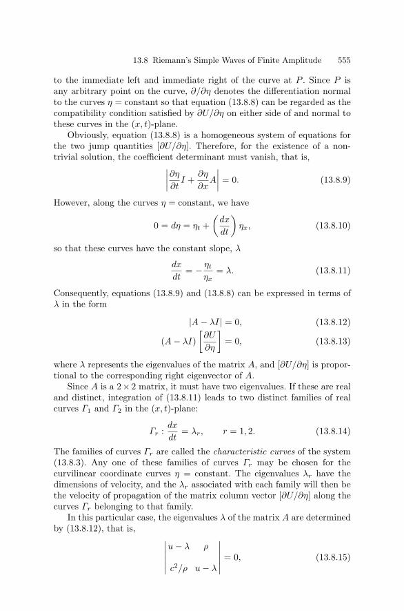
13.8 Riemann’s Simple Waves of Finite Amplitude 555
to the immediate left and immediate right of the curve at P . Since P isany arbitrary point on the curve, ∂/∂η denotes the differentiation normalto the curves η = constant so that equation (13.8.8) can be regarded as thecompatibility condition satisfied by ∂U/∂η on either side of and normal tothese curves in the (x, t)-plane.
Obviously, equation (13.8.8) is a homogeneous system of equations forthe two jump quantities [∂U/∂η]. Therefore, for the existence of a non-trivial solution, the coefficient determinant must vanish, that is,∣∣∣∣∂η
∂tI +
∂η
∂xA
∣∣∣∣ = 0. (13.8.9)
However, along the curves η = constant, we have
0 = dη = ηt +(
dx
dt
)ηx, (13.8.10)
so that these curves have the constant slope, λ
dx
dt= − ηt
ηx= λ. (13.8.11)
Consequently, equations (13.8.9) and (13.8.8) can be expressed in terms ofλ in the form
|A − λI| = 0, (13.8.12)
(A − λI)[∂U
∂η
]= 0, (13.8.13)
where λ represents the eigenvalues of the matrix A, and [∂U/∂η] is propor-tional to the corresponding right eigenvector of A.
Since A is a 2× 2 matrix, it must have two eigenvalues. If these are realand distinct, integration of (13.8.11) leads to two distinct families of realcurves Γ1 and Γ2 in the (x, t)-plane:
Γr :dx
dt= λr, r = 1, 2. (13.8.14)
The families of curves Γr are called the characteristic curves of the system(13.8.3). Any one of these families of curves Γr may be chosen for thecurvilinear coordinate curves η = constant. The eigenvalues λr have thedimensions of velocity, and the λr associated with each family will then bethe velocity of propagation of the matrix column vector [∂U/∂η] along thecurves Γr belonging to that family.
In this particular case, the eigenvalues λ of the matrix A are determinedby (13.8.12), that is, ∣∣∣∣∣∣
u − λ ρ
c2/ρ u − λ
∣∣∣∣∣∣ = 0, (13.8.15)

556 13 Nonlinear Partial Differential Equations with Applications
so that
λ = λr = u+c, r = 1, 2. (13.8.16)
Consequently, the families of the characteristic curves Γr (r = 1, 2) definedby (13.8.14) become
Γ1 :dx
dt= u + c, and Γ2 :
dx
dt= u − c. (13.8.17)
In physical terms, these results indicate that disturbances propagatewith the sum of the velocities of the fluid and sound along the family ofcurves Γ1. In the second family Γ2, they propagate with the difference ofthe fluid velocity u and the sound velocity c.
The right eigenvectors µr ≡
⎛⎜⎝µ(1)r
µ(2)r
⎞⎟⎠ are solutions of the equations
(A − λrI) µr = 0, r = 1, 2, (13.8.18)
or, ⎛⎝u − λr ρ
c2/ρ u − λr
⎞⎠⎛⎜⎝µ
(1)r
µ(2)r
⎞⎟⎠ = 0, r = 1, 2. (13.8.19)
This result combined with (13.8.13) gives⎛⎝ [ρη]
[uη]
⎞⎠ =
⎛⎜⎝µ(1)r
µ(2)r
⎞⎟⎠ = α
⎛⎝ 1
+ c/ρ
⎞⎠ , r = 1, 2, (13.8.20)
where α is a constant.In other words, across a wavefront in the Γ1 family of characteristic
curves,
[∂ρ/∂η]1
=[∂u/∂η]
c/ρ, (13.8.21)
and across a wavefront in the Γ2 family of characteristic curves,
[∂ρ/∂η]1
=[∂u/∂η]−c/ρ
, (13.8.22)
where c and ρ have values appropriate to the wavefront.The above method of characteristics can be applied to a more general
system

13.8 Riemann’s Simple Waves of Finite Amplitude 557
∂U
∂t+ A
∂U
∂x= 0, (13.8.23)
where U is an n × 1 matrix with elements u1, u2, . . ., un and A is an n × nmatrix with elements aij . An argument similar to that given above leadsto n eigenvalues of (13.8.13). If these eigenvalues are real and distinct,integration of equations (13.8.14) with r = 1, 2, . . ., n gives n distinctfamilies of real curves Γr in the (x, t)-plane so that
Γr :dx
dt= λr, r = 1, 2, . . . n. (13.8.24)
When the eigenvalues λr of A are all real and distinct, there are n dis-tinct linearly independent right eigenvectors µr of A satisfying the equation
Aµr = λrµr,
where µr is an n × 1 matrix with elements µ(1)r , µ
(2)r , . . ., µ
(n)r . Then across
a wavefront belonging to the Γr family of characteristics, it turns out that
[∂u1/∂η]
µ(1)r
=[∂u2/∂η]
µ(2)r
= . . . =[∂un/∂η]
µ(n)r
, (13.8.25)
where the elements of µr are known on the wavefront.In order to introduce the Riemann invariants, we form the linear com-
bination of the eigenvectors (+c/ρ, 1) with equations (13.8.1)–(13.8.2) toobtain
+c
ρ(ρt + ρux + uρx) +
(ut + uux +
c2
ρρx
)= 0. (13.8.26)
We use ∂u/∂ρ = + c/ρ from (13.8.21)–(13.8.22) and rewrite (13.8.26) as
+c
ρ[ρt + (u + c) ρx] + [ut + (u + c) ux] = 0. (13.8.27)
In view of (13.8.17), equation (13.8.27) becomes
du +c
ρdρ = 0 on Γr, r = 1, 2, (13.8.28)
or,
d [F (ρ) +u] = 0 on Γr, (13.8.29)
where
F (ρ) =∫ ρ
ρ0
c (ρ)ρ
dρ. (13.8.30)
Integration of (13.8.29) gives

558 13 Nonlinear Partial Differential Equations with Applications
F (ρ) + u = 2r on Γ1 and F (ρ) − u = 2s on Γ2, (13.8.31)
where 2r and 2s are constants of integration on Γ1 and Γ2, respectively.The quantities r and s are called the Riemann invariants. As stated
above, r is an arbitrary constant on characteristics Γ1, and hence, in general,r will vary on each Γ2. Similarly, s is constant on each Γ2 but will vary onΓ1. It is natural to introduce r and s as new curvilinear coordinates. Since ris constant on Γ1, s can be treated as the parameter on Γ1. Similarly, r canbe regarded as the parameter on Γ2. Then, dx = (u + c) dt on Γr impliesthat
dx
ds= (u + c)
dt
dson Γ1, (13.8.32)
dx
dr= (u − c)
dt
dron Γ2. (13.8.33)
In fact, r is a constant on Γ1, and s is a constant on Γ2. Therefore, thederivatives in the two equations are really partial derivations with respectto s and r so that we can rewrite them as
∂x
∂s= (u + c)
∂t
∂s, (13.8.34)
∂x
∂r= (u − c)
∂t
∂r. (13.8.35)
These two first-order PDE’s can, in general, be solved for x = x (r, s),t = t (r, s), and then, by inversion, r and s as functions x and t can beobtained. Once this is done, we use (13.8.31) to determine u (x, t) and ρ (x, t)in terms of r and s as
u (x, t) = r − s, F (ρ) = r + s. (13.8.36)
When one of the Riemann invariants r and s is constant throughoutthe flow, the corresponding solution is tremendously simplified. The solu-tions are known as simple wave motions representing simple waves in onedirection only. The generating mechanisms of simple waves with their prop-agation laws can be illustrated by the piston problem in gas dynamics.
Example 13.8.1. Determine the Riemann invariants for a polytropic gascharacterized by the law p = kργ , where k and γ are constants.
In this case
c2 =dp
dρ= kγργ−1, F (ρ) =
∫ ρ
0
c (ρ)ρ
=2c
γ − 1.
Hence, the Riemann invariants are given by(2c
γ − 1
)c + u = (2r, 2s) on Γr. (13.8.37)

13.8 Riemann’s Simple Waves of Finite Amplitude 559
It is also possible to express the dependent variables u and c in termsof the Riemann invariants. It turns out that
u = r − s, c =γ − 1
2(r + s) . (13.8.38)
Example 13.8.2. (The Piston Problem in a Polytropic Gas). The problemis to determine how a simple wave is produced by the prescribed motion ofa piston in the closed end of a semi-infinite tube filled with gas.
This is a one-dimensional unsteady problem in gas dynamics. We assumethat the gas is initially at rest with a uniform state u = 0, ρ = ρ0, andc = c0. The piston starts from rest at the origin and is allowed to withdrawfrom the tube with a variable velocity for a time t1, after which the velocityof withdrawal remains constant. The piston path is shown by a dottedcurve in Figure 13.8.1. In the (x, t)-plane, the path of the piston is givenby x = X (t) with X (0) = 0. The fluid velocity u is equal to the pistonvelocity X (t) on the piston x = X (t), which will be used as the boundarycondition for the piston.
The initial state of the gas is given by u = u0, ρ = ρ0, and c = c0at t = 0, in x ≥ 0. The characteristic line Γ0 that bounds it and passesthrough the origin is determined by the equation
dx
dt= (u + c)t=0 = c0
so that the equation of the characteristic line Γ0 is x = c0t.
Figure 13.8.1 Simple waves generated by the motion of a piston.

560 13 Nonlinear Partial Differential Equations with Applications
In view of the uniform initial state, all the Γ2 characteristics start onthe x-axis so that the Riemann invariants s in (12.8.37b) must be constantand of the form
2c
γ − 1− u =
2c0
γ − 1, (13.8.39)
or,
u =2 (c − c0)
γ − 1, c = c0 +
(γ − 1)2
u. (13.8.40ab)
The characteristics Γ1 meeting the piston are given by
2c
γ − 1+ u = 2r on each Γ1 and Γ1 :
dx
dt= u + c, (13.8.41)
which is, since (13.8.40ab) holds everywhere,
u = constant onΓ1 and Γ1 :dx
dt= c0 +
12
(γ + 1)u. (13.8.42)
Since the flow is continuous with no shocks, u = 0 and c = c0 ahead ofand on Γ0, which separates those Γ1 meeting the x-axis from those meet-ing the piston. The family of lines Γ1 through the origin has the equation(dx/dt) = ξ, where ξ is a parameter with ξ = c0 on Γ0. The Γ1 characteris-tics are also defined by (dx/dt) = u+c so that ξ = u+c. Hence, eliminationof c from (13.8.40b) gives
u =(
2γ + 1
)(ξ − c0) . (13.8.43)
Substituting this value of u in (13.8.40b), we obtain
c =(
γ − 1γ + 1
)ξ +
2c0
γ + 1. (13.8.44)
It follows from c2 = γ k ργ−1 and (13.8.40b) with the initial data, ρ = ρ0,c = c0 that
ρ = ρ0
[1 +
γ − 12c0
u
]2/(γ−1)
. (13.8.45)
With ξ = (x/t), results (13.8.43) through (13.8.45) give the completesolution of the piston problem in terms of x and t.
Finally, the equation of the characteristic line Γ1 is found by integratingthe second equation of (13.8.42) and using the boundary condition on thepiston. When a line Γ1 intersects the piston path at time t = τ , thenu = X (τ) along it, and the equation becomes

13.9 Discontinuous Solutions and Shock Waves 561
x = X (τ) +
c0 +γ + 1
2X (τ)
(t − τ) . (13.8.46)
It is noted that the family Γ1 represents straight lines with slope dx/dtincreasing with velocity u. Consequently, the characteristics are likely tooverlap on the piston, that is, X (τ) > 0 for any τ . If u increases, so do c,ρ, and p so that instability develops. It shows that shocks will be formed inthe compressive part of the disturbance.
13.9 Discontinuous Solutions and Shock Waves
The development of a nonunique solution of a nonlinear hyperbolic equationhas already been discussed in connection with several different problems. Inreal physical situations, this nonuniqueness usually manifests itself in theformation of discontinuous solutions which propagate in the medium. Suchdiscontinuous solutions across some surface are called shock waves. Thesewaves are found to occur widely in high speed flows in gas dynamics.
In order to investigate the nature of discontinuous solutions, we recon-sider the nonlinear conservation equation (13.6.5) that is,
∂ρ
∂t+
∂q
∂x= 0. (13.9.1)
This equation has been solved under two basic assumptions: (i) There existsa functional relation between q and ρ, that is, q = Q (ρ); (ii) ρ and qare continuously differentiable. In some physical situations, the solution of(13.9.1) leads to breaking phenomenon. When breaking occurs, questionsarise about the validity of these assumptions. To examine the formationof discontinuities, we consider the following: (a) we assume the relationq = Q (ρ) but allow jump discontinuity for ρ and q; (b) in addition to thefact that ρ and q are continuously differentiable, we assume that q is afunction of ρ and ρx. One of the simplest forms is
q = Q (ρ) − νρx, ν > 0. (13.9.2)
In case (a), we assume the conservation equation (13.6.1) still holds andhas the form
d
dt
∫ x2
x1
ρ (x, t) dx + q (x2, t) − q (x1, t) = 0. (13.9.3)
We now assume that there is a discontinuity at x = s (t) where s is acontinuously differentiable function of t, and x1 and x2 are chosen so thatx2 > s (t) > x1, and U (t) = s (t). Equation (13.9.3) can be written as
d
dt
[∫ s−
x1
ρ dx +∫ x2
s+ρ dx
]+ q (x2, t) − q (x1, t) = 0,

562 13 Nonlinear Partial Differential Equations with Applications
which implies that∫ s−
x1
ρt dx + sρ(s−, t
)+
∫ x2
s+ρt dx − sρ
(s+, t
)+ q (x2, t) − q (x1, t) = 0,
(13.9.4)
where ρ (s−, t), ρ (s+, t) are the values of ρ (x, t) as x → s from below andabove respectively. Since ρt is bounded in each of the intervals separately,the integrals tend to zero as x1 → s− and x2 → s+. Thus, in the limit,
q(s+, t
) − q(s−, t
)= U
ρ(s+, t
) − ρ(s−, t
). (13.9.5)
In the conventional notation of shock dynamics, this can be written as
q2 − q1 = U (ρ2 − ρ1) , (13.9.6)
or
−U [ρ] + [q] = 0, (13.9.7)
where subscripts 1 and 2 are used to denote the values behind and aheadof the shock respectively, and [ ] denotes the discontinuous jump in thequantity involved. Equation (13.9.7) is called the shock condition. Thus, thebasic problem can be written as
∂ρ
∂t+
∂q
∂x= 0 at points of continuity, (13.9.8)
−U [ρ] + [q] = 0 at points of discontinuity. (13.9.9)
Therefore, we have a nice correspondence
∂ρ
∂t↔ −U [ ] ,
∂
∂x↔ [ ] , (13.9.10)
between the differential equation and the shock condition.It is now possible to find discontinuous solutions of (13.9.3). In any
continuous part of the solution, equation (13.9.1) is still satisfied and theassumption q = Q (ρ) remains valid. But we have q1 = Q (ρ1) and q2 =Q (ρ2) on the two sides of any shock, and the shock condition (13.9.6) hasthe form
U (ρ2 − ρ1) = Q (ρ2) − Q (ρ1) . (13.9.11)
Example 13.9.1. The simplest example in which breaking occurs is
ρt + c (ρ) ρx = 0,
with discontinuous initial data at t = 0

13.10 Structure of Shock Waves and Burgers’ Equation 563
ρ =
⎧⎨⎩ρ2, x < 0
ρ1, x > 0, (13.9.12)
and
F (x) =
⎧⎨⎩c2 = c2 (ρ) , x < 0
c1 = c1 (ρ) , x > 0, (13.9.13)
where
ρ1 > ρ2 and c2 > c1.
In this case, breaking will occur immediately and this can be seen fromFigure 13.9.1ab with c′ (ρ) > 0. The multivalued region begins at the originξ = 0 and is bounded by the characteristics x = c1t and x = c2t withc1 < c2. This corresponds to a centered compression wave with overlappingcharacteristics in the (x, t)-plane.
On the other hand, if the initial condition is expansive with c2 < c1,there is a continuous solution obtained from (13.2.12) in which all valuesof F (x) in [c2, c1] are taken on characteristics through the origin ξ = 0.This corresponds to a centered fan of characteristics x = ct, c2 ≤ c ≤ c1in the (x, t)-plane so that the solution has the explicit form c = (x/t),c2 < (x/t) < c1. The density distribution and the expansion wave areshown in Figure 13.9.2ab.
In this case, the complete solution is given by
c =
⎧⎪⎪⎪⎪⎪⎨⎪⎪⎪⎪⎪⎩
c2, x ≤ c2t
x
t, c2t < x < c1t
c1, x ≥ c1t.
(13.9.14)
13.10 Structure of Shock Waves and Burgers’ Equation
In order to resolve breaking, we assumed a functional relation in ρ and qwith appropriate shock conditions. Now we investigate the case when
q = Q (ρ) − νρx, ν > 0. (13.10.1)
Note that near breaking where ρx is large, (13.10.1) gives a better approx-imation. With (13.10.1), the basic equation (13.9.1) becomes
ρt + c (ρ) ρx = νρxx, (13.10.2)

564 13 Nonlinear Partial Differential Equations with Applications
Figure 13.9.1ab Density distribution and centered compression wave with over-lapping characteristics.

13.10 Structure of Shock Waves and Burgers’ Equation 565
Figure 13.9.2ab Density distribution and centered expansion wave.

566 13 Nonlinear Partial Differential Equations with Applications
where c (ρ) = Q′ (ρ), the second and the third terms represent the effectson nonlinearity and diffusion.
We first solve (13.10.2) for two simple cases: (i) c (ρ) = constant = c,and (ii) c (ρ) ≡ 0. In the first case, equation (13.10.1) becomes linear andwe seek a plane wave solution
ρ (x, t) = a exp i (kx − ωt) . (13.10.3)
Substituting this solution into the linear equation (13.10.2), we have thedispersion relation
ω = ck − iνk2, (13.10.4)
where
Im ω = −νk2 < 0, since ν > 0.
Thus, the wave profile has the form
ρ (x, t) = a e−νk2t exp [ik (x − ct)] (13.10.5)
which represents a diffusive wave (Im ω < 0) with wavenumbers k and phasevelocity c whose amplitude decays exponentially with time t. The decaytime is given by t0 =
(νk2
)−1 which becomes smaller and smaller as kincreases with fixed ν. Thus, the waves of smaller wavelengths decay fasterthan waves of longer wavelengths. On the other hand, for a fixed wavenum-ber k, t0 decreases as ν increases so that waves of a given wavelength atten-uate faster in a medium with larger ν. The quantity ν may be regarded asa measure of diffusion. Finally, after a sufficiently long time (t t0) onlydisturbances of long wavelength will survive, while all short wavelengthdisturbances will decay rapidly.
In the second case, (13.10.2) reduces to the linear diffusion equation
ρt = νρxx. (13.10.6)
This equation with the initial data at t = 0
ρ =
⎧⎨⎩ρ1, x < 0
ρ1, x > 0,ρ1 > ρ2, (13.10.7)
can readily be solved, and the solution for t > 0 is
ρ (x, t) =ρ1
2√
πνt
∫ 0
−∞e−(x−ξ)2/4νtdξ +
ρ2
2√
πνt
∫ ∞
0e−(x−ξ)2/4νtdξ.
(13.10.8)
After some manipulation involving changes of variables of integration(x − ξ) /2
√νt = η, the solution is simplified to the form

13.10 Structure of Shock Waves and Burgers’ Equation 567
u (x, t) =12
(ρ1 + ρ2) + (ρ2 − ρ1)1√π
∫ x/2√
νt
0e−η2
dη, (13.10.9)
=12
(ρ1 + ρ2) +12
(ρ2 − ρ1) erf(
x
2√
νt
). (13.10.10)
This shows that the effect of the term νρxx is to smooth out the initialdistribution (νt)− 1
2 . The solution tends to values ρ1, ρ2 as x → + ∞. Theabsence of the term νρxx in (13.10.2) leads to nonlinear steepening andbreaking. Indeed, equation (13.10.2) combines the two opposite effects ofbreaking and diffusion. The sign of ν is important; indeed, solutions arestable or unstable according as ν > 0 or ν < 0.
In order to investigate solutions that balance between steepening anddiffusion, we seek solutions of (13.10.2) in the form
ρ = ρ (X) , X = x − Ut, (13.10.11)
where U is a constant to be determined.It follows from (13.10.2) that
[c (ρ) − U ] ρX = νρXX . (13.10.12)
Integrating this equation gives
Q (ρ) − Uρ + A = νρX , (13.10.13)
where A is a constant of integration.Integrating (13.10.13) with respect to X gives an implicit relation for
ρ (X) in the form
X
ν=
∫dρ
Q (ρ) − Uρ + A. (13.10.14)
We would like to have a solution which tends to ρ1, ρ2 as X → + ∞. Ifsuch a solution exists with ρX → 0 as |X| → ∞, the quantities U and Amust satisfy
Q (ρ1) − Uρ1 + A = Q (ρ2) − Uρ2 + A = 0, (13.10.15)
which implies that
U =Q (ρ1) − Q (ρ2)
ρ1 − ρ2. (13.10.16)
This is exactly the same as the shock velocity obtained before.Result (13.10.15) shows that ρ1, ρ2 are zeros of Q (ρ) − Uρ + A. In
the limit ρ → ρ1 or ρ2, the integral (13.10.14) diverges and X → + ∞. Ifc′ (ρ) > 0, then Q (ρ)−Uρ+A ≤ 0 in ρ2 ≤ ρ ≤ ρ1 and then ρX ≤ 0 because

568 13 Nonlinear Partial Differential Equations with Applications
Figure 13.10.1 Shock structure and shock thickness.
of (13.10.11). Thus, ρ decreases monotonically from ρ1 at X = −∞ to ρ2at X = ∞ as shown in Figure 13.10.1.
Physically, a continuous waveform carrying an increase in ρ will progres-sively distort itself and eventually break forward and require a shock withρ1 < ρ2 provided c′ (ρ) > 0. It will break backward and require a shockwith ρ1 > ρ2 and c′ (ρ) < 0.
Example 13.10.1. Obtain the solution of (13.10.2) with the initial data(13.10.7) and Q (ρ) = αρ2 + βρ + γ, α > 0.
We write
Q (ρ) − Uρ + A = −α (ρ1 − ρ) (ρ − ρ2) ,
where
U = β + α (ρ1 + ρ2) and A = αρ1ρ2 − γ.
Integral (13.10.14) becomes
X
ν= − 1
α
∫dρ
(ρ − ρ2) (ρ1 − ρ)=
1α (ρ1 − ρ2)
log(
ρ1 − ρ
ρ − ρ2
),
which gives the solution
ρ (X) = ρ2 + (ρ1 − ρ2)exp
[αXν (ρ2 − ρ1)
]1 + exp
[αXν (ρ2 − ρ1)
] . (13.10.17)

13.10 Structure of Shock Waves and Burgers’ Equation 569
The exponential factor in the solution indicates the existence of a tran-sition layer of thickness δ of the order of ν/ [α (ρ1 − ρ2)]. This can also bereferred to as the shock thickness. The thickness δ increases as ρ1 → ρ2 fora fixed ν. It tends to zero as ν → 0 for a fixed ρ1 and ρ2.
In this case, the shock velocity (13.10.16) becomes
U = α (ρ1 − ρ2) + β =12
(c1 + c2) , (13.10.18)
where c (ρ) = Q′ (ρ), c1 = c (ρ1), and c2 = c (ρ2).We multiply (13.10.2) by c′ (ρ) and simplify to obtain
ct + ccx = νcxx − ν c′′ (ρ) ρ2x. (13.10.19)
Since Q (ρ) is a quadratic expression in ρ, then c (ρ) = Q′ (ρ) becomeslinear in ρ and c′′ (ρ) = 0. Thus, (13.10.19) leads to Burgers’ equationreplacing c with u
ut + uux = ν uxx. (13.10.20)
This equation incorporates the combined opposite effects of nonlinearityand diffusion. It is the simplest nonlinear model equation for diffusive wavesin fluid dynamics. Using the Cole–Hopf transformation
u = −2νφx
φ. (13.10.21)
Burgers’ equation can be solved exactly, and the opposite effects of nonlin-earity and diffusion can be investigated in some detail.
We introduce the transformation in two steps. First, we write u = ψx
so that (13.10.20) can readily be integrated to obtain
ψt +12ψ2
x = ν ψxx. (13.10.22)
The next step is to introduce ψ = −2ν log φ and to transform thisequation into the so called diffusion equation
φt = ν φxx. (13.10.23)
This equation was solved in earlier chapters. We simply quote the solu-tion of the initial-value problem of (13.10.23) with the initial data
φ (x, 0) = Φ (x) , −∞ < x < ∞. (13.10.24)
The solution for φ is
φ (x, t) =1
2√
πνt
∫ ∞
−∞Φ (ζ) exp
[− (x − ζ)2
4νt
]dζ, (13.10.25)

570 13 Nonlinear Partial Differential Equations with Applications
where Φ (ζ) can be written in terms of the initial value u (x, 0) = F (x) byusing (13.10.21). It turns out that, at t = 0,
φ (x, t) = Φ (x) = exp
− 12ν
∫ x
0F (α) dα
. (13.10.26)
It is then convenient to write down φ (x, t) in the form
φ (x, t) =1
2√
πνt
∫ ∞
−∞exp
(− f
2ν
)dζ, (13.10.27)
where
f (ζ, x, t) =∫ ζ
0F (α) dα +
(x − ζ)2
2t. (13.10.28)
Consequently,
φx (x, t) = − 14ν
√πνt
∫ ∞
−∞
(x − ζ)t
exp(
− f
2ν
)dζ. (13.10.29)
Therefore, the solution for u follows from (13.10.21) and has the form
u (x, t) =
∫ ∞−∞
(x−ζ
t
)exp
(− f
2ν
)dζ∫ ∞
−∞ exp(− f
2ν
)dζ
. (13.10.30)
Although this is the exact solution of Burgers’ equation, physical inter-pretation can hardly be given unless a suitably simple form of F (x) is spec-ified. Even then, finding an exact evaluation of the integrals in (13.10.30)is a formidable task. It is then necessary to resort to asymptotic methods.Before we deal with asymptotic analysis, the following example may beconsidered for an investigation of shock formation.
Example 13.10.2. Find the solution of Burgers’ equation with physical sig-nificance for the case
F (x) =
⎧⎨⎩A δ (x) , x < 0
0, x > 0.
We first find
f (ζ, x, t) = A
∫ ζ
0+δ (α) dα +
(x − ζ)2
t
=
⎧⎪⎨⎪⎩(x−ζ)2
2t − A, ζ < 0
(x−ζ)2
2t , ζ > 0.

13.10 Structure of Shock Waves and Burgers’ Equation 571
Thus,∫ ∞
−∞
x − ζ
texp
(− f
2ν
)dζ =
∫ 0
−∞
(x − ζ
t
)exp
[A
2ν− (x − ζ)2
4νt
]dζ
+∫ ∞
0
(x − ζ
t
)exp
[− (x − ζ)2
4νt
]dζ
= 2ν(eA/2ν − 1
)exp
(− x2
4νt
),
which is obtained by substitution,
x − ζ
2√
νt= α.
Similarly,∫ ∞
−∞exp
(− f
2ν
)dζ = 2
√νt
[√π +
(eA/2ν − 1
)erfc
(x
2√
νt
)],
where erfc (x) is the complementary error function defined by
erfc (x) =2√π
∫ ∞
x
e−η2dη. (13.10.31)
Therefore, the solution for u (x, t) is
u (x, t) =√
ν
t
(eA/2ν − 1
)exp
(− x2
4νt
)√
π +(eA/2ν − 1
)(√
π/2) erfc(
x2√
νt
) . (13.10.32)
In the limit as ν → ∞, the effect of diffusion would be more significantthan that of nonlinearity. Since
erfc(
x
2√
νt
)→ 0, eA/2ν ∼ 1 +
A
2νas ν → ∞,
the solution (13.10.32) tends to the limiting value
u (x, t) ∼ A
2√
πνtexp
(− x2
4νt
). (13.10.33)
This represents the well-known source solution of the classical linear heatequation ut = ν uxx.
On the other hand, when ν → 0 nonlinearity would dominate overdiffusion. It is expected that solution (13.10.32) tends to that of Burgers’equation as ν → 0.

572 13 Nonlinear Partial Differential Equations with Applications
We next introduce the similarity variable η = x/√
2At to rewrite(13.10.32) in the form
u (x, t) =(ν
t
) 12
(eA/2ν − 1
)exp
(−Aη2
2ν
)√
π +(eA/2ν − 1
)(√
π/2) erfc(√
A2ν η
) , (13.10.34)
∼(ν
t
) 12 exp
A2ν
(1 − η2
)√
π + (√
π/2) exp(
A2ν
)erfc
(√A2ν η
) as ν → 0 for all η,
(13.10.35)∼ 0 as ν → 0, for η < 0 and η > 1. (13.10.36)
Invoking the asymptotic result,
erfc (x) ∼ (2/
√π) e−x2
2xas x → ∞, (13.10.37)
the solution (13.10.34) for 0 < η < 1 has the form,
u (x, t) ∼(ν
t
) 12 2η
(A2ν
) 12 exp
A2ν
(1 − η2
)2η
(Aπ2ν
) 12 + exp
A2ν (1 − η2)
.
=(
2A
t
) 12 η
1 + 2η(
Aπ2ν
) 12 exp
A2ν (η2 − 1)
∼
(2A
t
) 12
as ν → 0.
The final asymptotic solution as ν → 0 is
u (x, t) ∼⎧⎨⎩
xt , 0 < x < (2At)
12
0, otherwise.(13.10.38)
This result represents a shock at x = (2At)12 with the velocity U = (A/2t)
12 .
This solution u has a jump from 0 to x/t = (2A/t)12 so that the shock
condition is fulfilled.
Asymptotic Behavior of Burgers’ Solution as ν → 0.
We use the Kelvin stationary phase approximation method discussed inSection 12.7 to examine the asymptotic behavior of Burgers’ solution(13.10.30). According to this method, the significant contribution to theintegrals involved in (13.10.30) comes from points of stationary phase forfixed x and t, that is, from the roots of the equation

13.11 The Korteweg–de Vries Equation and Solitons 573
∂f
∂ζ= F (ζ) − (x − ζ)
t= 0. (13.10.39)
Suppose that ζ = ξ (x, t) is a root. According to result (12.7.8), integralsin (13.10.30) as ν → 0 yield∫ ∞
−∞
(x − ξ
t
)exp
(− f
2ν
)dζ ∼ x − ξ
t
4πν
|f ′′ (ξ)| 1
2
exp
−f (ξ)2ν
∫ ∞
−∞exp
(− f
2ν
)dζ ∼
4πν
|f ′′ (ξ)| 1
2
exp
−f (ξ)2ν
.
Therefore, the final asymptotic solution is
u (x, t) ∼ x − ξ
t, (13.10.40)
where ξ satisfies (13.10.39). In other words, the solution can be rewrittenin the form
ux
==
F (ξ)ξ + tF (ξ)
. (13.10.41)
This is identical with the solution (13.2.12) which was obtained in Sec-tion 13.2. In this case, the stationary point ξ represents the characteristicvariable.
Although the exact solution of Burgers’ equation is a single-valued andcontinuous function for all time t, the asymptotic solution (13.10.41) ex-hibits instability. It has already been shown that (13.10.41) progressivelydistorts itself and becomes multiple-valued after sufficiently long time.Eventually, breaking will definitely occur.
It follows from the analysis of Burgers’ equation that the nonlinear anddiffusion terms show opposite effects. The former introduces steepening inthe solution profile, whereas the latter tends to diffuse (spread) the sharpdiscontinuities into a smooth profile. In view of this property, the solutionrepresents the diffusive wave. In the context of fluid flows, ν denotes thekinematic viscosity which measures the viscous dissipation.
Finally, Burgers’ equation arises in many physical problems, includ-ing one-dimensional turbulence (where this equation had its origin), soundwaves in viscous media, shock waves in viscous media, waves in fluid-filledviscous elastic pipes, and magnetohydrodynamic waves in media with finiteconductivity.
13.11 The Korteweg–de Vries Equation and Solitons
The celebrated dispersion relation (13.3.14) for dispersive surface waves onwater of constant depth h0 is

574 13 Nonlinear Partial Differential Equations with Applications
ω = (gk tanh kh0)12
= c0k
(1 − 1
3k2h2
0
) 12
≈ c0k
(1 − 1
6k2h2
0
), (13.11.1)
where c0 = (gh0)12 is the shallow water wave speed.
In many physical problems, wave motions with small dispersion exhibitsuch a k2 term in contrast to the linearized theory value of c0k. An equationfor the free surface elevation η (x, t) with this dispersion relation is givenby
ηt + c0ηx + σηxxx = 0, (13.11.2)
where σ = 16c0h
20 is a constant for fairly long waves. This equation is called
the linearized Korteweg–de Vries (KdV) equation for fairly long waves mov-ing to the positive x direction only. The phase and group velocities of thewaves are found from (13.11.1) and they are given by
Cp =ω
k= c0 − σk2, (13.11.3)
Cg =dω
dk= c0 − 3σk2. (13.11.4)
It is noted that Cp > Cg, and the dispersion comes from the term involvingk3 in the dispersion relation (13.11.1) and hence, from the term σηxxx. Forsufficiently long waves (k → 0), Cp = Cg = c0, and hence, these waves arenondispersive.
In 1895, Korteweg–de Vries derived the nonlinear equation for long wa-ter waves in a channel of depth h0 which has the remarkable form
ηt + c0
(1 +
32
η
h0
)ηx + σηxxx = 0. (13.11.5)
This is the simplest nonlinear model equation for dispersive waves, andcombines nonlinearity and dispersion. The KdV equation arises in manyphysical problems, which include water waves of long wavelengths, plasmawaves, and magnetohydynamics waves. Like Burgers’ equation, the nonlin-earity and dispersion have opposite effects on the KdV equation. The formerintroduces steepening of the wave profile while the latter counteracts wave-form steepening. The most remarkable features is that the dispersive termin the KdV equation does allow the solitary and periodic waves which arenot found in shallow water wave theory. In Burgers’ equation the nonlinearterm leads to steepening which produces a shock wave; on the other hand,in the KdV equation the steepening process is balanced by dispersion togive a rise to a steady solitary wave.
We now seek the traveling wave solution of the KdV equation (13.11.5)in the form

13.11 The Korteweg–de Vries Equation and Solitons 575
η (x, t) = h0f (X) , X = x − Ut, (13.11.6)
for some function f and constant wave velocity U . We determine f andU by substitution of the form (13.11.6) into (13.11.5). This gives, withσ = 1
6c0h20,
16
h20f
′′′ +32ff ′ +
(1 − U
c0
)f ′ = 0, (13.11.7)
and then integration leads to
16
h20f
′′ +34
f2 +(
1 − U
c0
)f + A = 0,
where A is an integrating constant.We next multiply this equation by f ′ and integrate again to obtain
13h2
0f′2 + f3 + 2
(1 − U
c0
)f2 + 4 Af + B = 0, (13.11.8)
where B is a constant of integration.We now seek a solitary wave solution under the boundary conditions f ,
f ′, f ′′ → 0 as |X| → ∞. Therefore, A = B = 0 and (13.11.8) assumes theform
13
h20f
′2 + f2 (f − α) = 0, (13.11.9)
where
α = 2(
U
c0− 1
). (13.11.10)
Finally, we obtain
X =∫ f
0
df
f ′ =(
h20
3
) 12∫ f
0
df
f√
(α − f),
which is, by the substitution f = α sech2θ,
X − X0 =(
4h20
3α
) 12
θ, (13.11.11)
for some integrating constant X0.Therefore, the solution for f (X) is
f (X) = α sech2
[(3α
4h20
) 12
(X − X0)
]. (13.11.12)

576 13 Nonlinear Partial Differential Equations with Applications
Figure 13.11.1 A soliton.
The solution f (X) increases from f = 0 as X → −∞ so that it attains amaximum value f = fmax = α at X = 0, and then decreases symmetricallyto f = 0 as X → ∞ as shown in Figure 13.11.1. These features also implythat X0 = 0, so that (13.11.12) becomes
f (X) = α sech2
[(3α
4h20
) 12
X
]. (13.11.13)
Therefore, the final solution is
η (x, t) = η0 sech2
[(3η0
4h30
) 12
(x − Ut)
], (13.11.14)
where η0 = (αh0). This is called the solitary wave solution of the KdVequation for any positive constant η0. However, it has come to be known assoliton since Zabusky and Kruskal coined the term in 1965. Since η > 0 forall X, the soliton is a wave of elevation which is symmetrical about X = 0.It propagates in the medium without change of shape with velocity
U = c0
(1 +
α
2
)= c0
(1 +
12
η0
h0
), (13.11.15)
which is directly proportional to the amplitude η0. The width,(3η0/4h3
0)− 1
2
is inversely proportional to√
η0. In other words, the solitary wave propa-gates to the right with a velocity U which is directly proportional to theamplitude, and has a width that is inversely proportional to the square rootof the amplitude. Therefore, taller solitons travel faster and are narrowerthan the shorter (or slower) ones. They can overtake the shorter ones, andsurprisingly, they emerge from the interaction without change of shape asshown in Figure 13.11.2. Indeed the discovery of soliton interactions con-firms that solitons behave like elementary particles.
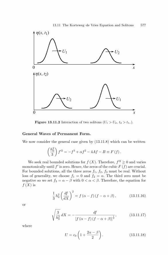
13.11 The Korteweg–de Vries Equation and Solitons 577
Figure 13.11.2 Interaction of two solitons (U1 > U2, t2 > t1, ).
General Waves of Permanent Form.
We now consider the general case given by (13.11.8) which can be written(h2
0
3
)f ′2 = −f3 + αf2 − 4Af − B ≡ F (f) .
We seek real bounded solutions for f (X). Therefore, f ′2 ≥ 0 and variesmonotonically until f ′ is zero. Hence, the zeros of the cubic F (f) are crucial.For bounded solutions, all the three zeros f1, f2, f3 must be real. Withoutloss of generality, we choose f1 = 0 and f2 = α. The third zero must benegative so we set f3 = α − β with 0 < α < β. Therefore, the equation forf (X) is
13
h20
(df
dX
)2
= f (α − f) (f − α + β) , (13.11.16)
or √3h2
0dX = − df
[f (α − f) (f − α + β)]12, (13.11.17)
where
U = c0
(1 +
2α − β
2
). (13.11.18)

578 13 Nonlinear Partial Differential Equations with Applications
We put α − f = p2 in (13.11.17) to obtain(3
4h20
) 12
dX =dp
[(α − p2) (β − p2)]12. (13.11.19)
We next substitute p =√
α q into (13.11.19) to transform it into thestandard form (
3β
4h20
) 12
X =∫ q
0
dq
[(1 − q2) (1 − m2q2)]12
(13.11.20)
where m = (α/β)12 .
The right hand side is an integral of the first kind, and hence, q canbe expressed in terms of the Jacobian sn function (see Dutta and Debnath(1965))
q = sn
[(3β
4h20
) 12
X, m
], (13.11.21)
where m is the modulus of the Jacobian elliptic function sn (z, m). There-fore,
f (X) = α
[1 − sn2
(3β
4h20
) 12
X
]
= α cn2
[(3β
4h20
) 12
X
], (13.11.22)
where cn (z, m) is also the Jacobian elliptic function of modulus m andcn2 (z) = 1 − sn2 (z).
From (13.11.20), the period P is given by
P = 2(
4h20
3β
) 12∫ 1
0
dq
[(1 − q2) (1 − m2q2)]12
(13.11.23)
=4h0√3β
K (m) ≡ λ, (13.11.24)
where K (m) is the complete elliptic integral of the first kind defined by
K (m) =∫ π/2
0
(1 − m sin2 θ
)− 12 dθ (13.11.25)
and λ denotes the wavelength of the cnoidal wave.It is important to note that cn (z, m) is periodic, and hence, η (X) rep-
resents a train of periodic waves in shallow water. Thus, these waves arecalled cnoidal waves with wavelength

13.11 The Korteweg–de Vries Equation and Solitons 579
Figure 13.11.3 A cnoidal wave.
λ = 2(
4h3
3b
)1/2
K (m) . (13.11.26)
The outcome of this analysis is that solution (13.11.22) represents anonlinear wave whose shape and wavelength (or period) all depend on theamplitude of the wave. A typical cnoidal wave is shown in Figure 13.11.3.Sometimes, the cnoidal waves with slowly varying amplitude are observedin rivers. More often, wavetrains behind a weak bore (called an undularbore) can be regarded as cnoidal waves.
Two limiting cases are of special interest: (i) m → 1 and (ii) m → 0.When m → 1 (α → β), it is easy to show that cn (z) → sech z. Hence, the
cnoidal wave solution (13.11.22) tends to the solitary wave with the wave-length λ, given by (13.11.24) which approaches infinity because K (1) = ∞,K (0) = π/2. The solution identically reduces to (13.11.14) with (13.11.15).
In the other limit m → 0 (α → 0), sn z → sin z and cn z → cos z so thatsolution (13.11.22) becomes
f (X) = α cos2[(
3β
4h20
) 12
X
], (13.11.27)
where
U = c0
(1 − β
2
). (13.11.28)
Using cos 2θ = 2 cos2 θ − 1, we can rewrite (13.11.27) in the form
f (X) =α
2
[1 + cos
(√3β
h0
)X
]. (13.11.29)
We next introduce k =√
3β/h0 (or β = 13k2h2
0) to simplify (13.11.29) as
f (X) =α
2[1 + cos (kx − ωt)] , (13.11.30)
where
ω = Uk = c0k
(1 − 1
6k2h2
0
). (13.11.31)
This corresponds to the first two terms of the series of (gk tanh kh0)1/2.
Thus, these results are in perfect agreement with the linearized theory.
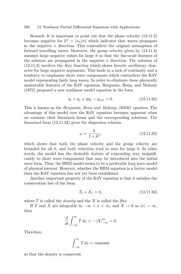
580 13 Nonlinear Partial Differential Equations with Applications
Remark: It is important to point out that the phase velocity (13.11.3)becomes negative for k2 > (c0/σ) which indicates that waves propagatein the negative x direction. This contradicts the original assumption offorward travelling waves. Moreover, the group velocity given by (13.11.4)assumes large negative values for large k so that the fine-scale features ofthe solution are propagated in the negative x direction. The solution of(13.11.2) involves the Airy function which shows fiercely oscillatory char-acter for large negative arguments. This leads to a lack of continuity and atendency to emphasize short wave components which contradicts the KdVmodel representing fairly long waves. In order to eliminate these physicallyundesirable features of the KdV equation, Benjamin, Bona, and Mahony(1972) proposed a new nonlinear model equation in the form
ηt + ηx + ηηx − ηxxt = 0. (13.11.32)
This is known as the Benjamin, Bona and Mahony (BBM) equation. Theadvantage of this model over the KdV equation becomes apparent whenwe examine their linearized forms and the corresponding solutions. Thelinearized form (13.11.32) gives the dispersion relation
ω =k
1 + k2 , (13.11.33)
which shows that both the phase velocity and the group velocity arebounded for all k, and both velocities tend to zero for large k. In otherwords, the model has the desirable feature of responding very insignifi-cantly to short wave components that may be introduced into the initialwave form. Thus, the BBM model seems to be a preferable long wave modelof physical interest. However, whether the BBM equation is a better modelthan the KdV equation has not yet been established.
Another important property of the KdV equation is that it satisfies theconservation law of the form
Tt + Xx = 0, (13.11.34)
where T is called the density and the X is called the flux.If T and X are integrable in −∞ < x < ∞, and X → 0 as |x| → ∞,
then
d
dt
∫ ∞
−∞T dx = − |X|∞−∞ = 0.
Therefore, ∫ ∞
−∞T dx = constant
so that the density is conserved.

13.12 The Nonlinear Schrodinger Equation and Solitary Waves 581
The canonical form of the KdV equation
ut − 6uux + uxxx = 0, (13.11.35)
can be written as
(u)t +(−3u2 + uxx
)x
= 0
so that
T = u and X = −3u2 + uxx. (13.11.36)
If we assume that u is periodic or that u and its derivatives decay veryrapidly as |x| → ∞, then
d
dt
∫ ∞
−∞u dx = 0.
This leads to the conservation of mass, that is,∫ ∞
−∞u dx = constant. (13.11.37)
This is often called the time invariant function of the solutions of the KdVequation.
The second conservation law for (13.11.34) can be obtained by multi-plying it by u so that(
12u2
)t
+(
−2u3 + uux − 12u2
x
)x
= 0. (13.11.38)
This gives ∫ ∞
−∞
12
u2dx = constant. (13.11.39)
This is the principle of conservation of energy.It is well known that the KdV equation has an infinite number of poly-
nomial conservation laws. It is generally believed that the existence of asoliton solution to the KdV equation is closely related to the existence ofan infinite number of conservation laws.
13.12 The Nonlinear Schrodinger Equation andSolitary Waves
We first derive the one-dimensional linear Schrodinger equation from theFourier integral representation of the plane wave solution

582 13 Nonlinear Partial Differential Equations with Applications
φ (x, t) =∫ ∞
−∞F (k) exp [i (kx − ωt)] dk, (13.12.1)
where the spectrum function F (k) is determined from the given initial orboundary conditions.
We assume that the wave is slowly modulated as it propagates in a dis-persive medium. For such a modulated wave, most of the energy is confinedin the neighborhood of k = k0 so that the dispersion relation ω = ω (k) canbe expanded about the point k = k0 as
ω = ω (k) = ω0 + (k − k0) ω′0 +
12
(k − k0)2ω′′
0 + . . . , (13.12.2)
where ω0 ≡ ω (k0), ω′0 ≡ ω′ (k0), ω′′
0 ≡ ω′′ (k0).In view of (13.12.2), we can rewrite (13.12.1) as
φ (x, t) = ψ (x, t) exp [i (k0x − ω0t)] , (13.12.3)
where the amplitude ψ (x, t) is given by
ψ (x, t) =∫ ∞
−∞F (k) exp
[i (k − k0) x − i
(k − k0) ω′
0
+12
(k − k0)2ω′′
0
t
]dk. (13.12.4)
Evidently, this represents the slowly varying (or modulated) part of thebasic wave. A simple computation of ψt, ψx, and ψxx gives
ψt = −i
(k − k0) ω′
0 +12
(k − k0)2ω′′
0
ψ
ψx = i (k − k0) ψ
ψxx = − (k − k0)2ψ
so that
i (ψt + ω′0 ψx) +
12
ω′′0 ψxx = 0. (13.12.5)
The dispersion relation associated with this linear equation is given by
ω = k ω′0 +
12
k2ω′′0 . (13.12.6)
If we choose a frame of reference moving with the linear group velocity,that is, x∗ = x − ω′
0 t, t∗ = t, the term involving ψx is dropped and then, ψsatisfies the linear Schrodinger equation, dropping the asterisks,

13.12 The Nonlinear Schrodinger Equation and Solitary Waves 583
i ψt +12
ω′′0 ψxx = 0. (13.12.7)
We next derive the nonlinear Schrodinger equation from the nonlineardispersion relation involving both frequency and amplitude in the mostgeneral form
ω = ω(k, a2) . (13.12.8)
We first expand ω in a Taylor series about k = k0 and |a|2 = 0 in theform
ω = ω0 + (k − k0)(
∂ω
∂k
)k=k0
+12
(k − k0)2(
∂2ω
∂k2
)k=k0
+
(∂ω
∂ |a|2)
|a|2=0
|a|2 , (13.12.9)
where ω0 ≡ ω (k0).If we now replace , ω − ω0 by i (∂/∂t) and k − k0 by −i (∂/∂x), and
assume that the resulting operators act on a, we obtain
i (at + ω′0 ax) +
12
ω′′0 axx + γ |a|2 a = 0, (13.12.10)
where
ω′0 ≡ ω′ (k0) , ω′′
0 ≡ ω′′ (k0) , and γ ≡ −(
∂ω
∂ |a|2)
|a|2=0
is a constant.
Equation (13.12.10) is known as the nonlinear Schrodinger (NLS) equa-tion. If we choose a frame of reference moving with the linear group velocityω′
0, that is, x∗ = x − ω′0 t and t∗ = t, the term involving ax will drop out
from (13.12.10), and the amplitude a (x, t) satisfies the normalized NLSequation, dropping the asterisks,
i at +12
ω′′0 axx + γ |a|2 a = 0. (13.12.11)
The corresponding dispersion relation is given by
ω =12
ω′′0 k2 − γ a2. (13.12.12)
According to the stability criterion established in Section 13.5, the wavemodulation is stable if γ ω′′
0 < 0 and unstable if γ ω′′0 > 0.
To study the solitary wave solution, it is convenient to use the NLSequation in the standard form
i ψt + ψxx + γ |ψ|2 ψ = 0, −∞ < x < ∞, t ≥ 0. (13.12.13)

584 13 Nonlinear Partial Differential Equations with Applications
We seek waves of permanent form by assuming the solution
ψ = f (X) ei(mX−nt), X = x − Ut (13.12.14)
for some functions f and constant wave speed U to be determined, and m,n are constants.
Substitution of (13.12.14) into (13.12.13) gives
f ′′ + i (2m − U) f ′ +(n − m2) f + γ |f |2 f = 0. (13.12.15)
We eliminate f ′ by setting 2m − U = 0, and then, write n = m2 − α sothat f can be assumed to be real. Thus, equation (13.12.15) becomes
f ′′ − αf + γ f3 = 0. (13.12.16)
Multiplying this equation by 2f ′ and integrating, we find that
f ′2 = A + αf2 − γ
2f4 ≡ F (f) , (13.12.17)
where F (f) ≡ (α1 − α2f
2) (
β1 − β2f2), so that α = − (α1β2 + α2β1),
A = α1β1, γ = −2 (α2β2), and α′s and β′s are assumed to be real anddistinct.
Evidently,
X =∫ f
0
df√(α1 − α2f2) (β1 − β2f2)
. (13.12.18)
Putting (α2/α1)12 f = u in this integral, we deduce the following elliptic
integral of the first kind (see Dutta and Debnath (1965)):
σX =∫ u
0
du√(1 − u2) (1 − κ2u2)
, (13.12.19)
where σ = (α2β1)12 and κ = (α1β2) / (β1α2).
Thus, the final solution can be expressed in terms of the Jacobian snfunction
u = sn (σX, κ) ,
or,
f (X) =(
α1
α2
) 12
sn (σX, κ) . (13.12.20)
In particular, when A = 0, α > 0, and γ > 0, we obtain a solitary wavesolution. In this case, equation (13.12.17) can be rewritten as

13.12 The Nonlinear Schrodinger Equation and Solitary Waves 585
√α X =
∫ f
0
df
f(1 − γ
2αf2) 1
2. (13.12.21)
Substitution of (γ/2α)12 f = sech θ in this integral gives the exact solution
f (X) =(
2α
γ
) 12
sech[√
α (x − Ut)]. (13.12.22)
This represents a solitary wave which propagates without change of shapewith constant velocity U . Unlike the solution of the KdV equation, theamplitude and the velocity of the wave are independent parameters. It isnoted that the solitary wave exists only for the unstable case (γ > 0). Thismeans that small modulations of the unstable wavetrain lead to a series ofsolitary waves.
The nonlinear dispersion relation for deep water waves is
ω =√
gk
(1 +
12a2k2
). (13.12.23)
Therefore,
ω′0 =
ω0
2k0, ω′′
0 = − ω0
4k20, and γ = −1
2ω0k
20, (13.12.24)
and the NLS equation for deep water waves is obtained from (13.12.10) inthe form
i
(at +
ω0
2k0ax
)−
(ω0
8k20
)axx − 1
2ω0 k2
0 |a|2 a = 0. (13.12.25)
The normalized form of this equation in a frame of reference moving withthe linear group velocity ω′
0 is
i at −(
ω0
8k20
)axx =
12
ω0 k20 |a|2 a. (13.12.26)
Since γ ω′′0 =
(ω2
0/8)
> 0, this equation confirms the instability of deepwater waves. This is one of the most remarkable recent results in the theoryof water waves.
We next discuss the uniform solution and the solitary wave solution of(13.12.26). We look for solutions in the form
a (x, t) = A (X) exp(i γ2 t
), X = x − ω′
0 t (13.12.27)
and substitute this into equation (13.12.26) to obtain
AXX = −(
8k20
ω0
)(γ2A +
12ω0 k2
0 A3)
. (13.12.28)

586 13 Nonlinear Partial Differential Equations with Applications
We multiply this equation by 2AX and then integrate to find
A2X = −
(A4
0 m′2 +8ω0
γ2k20A
2 + 2k40A
4)
=(A2
0 − A2) (A2 − m′2A2
0), (13.12.29)
where(A4
0m′2) is an integrating constant and 2k4
0 = 1, m′2 = 1 − m2, andA2
0 = 4γ2/ω0k20(m2 − 2
)which relates A0, γ, and m.
Finally, we rewrite equation (13.12.29) in the form
A20 dX =
dA[(1 − A2
A20
)(A2
A20
− m′2)] 1
2, (13.12.30)
or,
A0 (X − X0) =∫ ′ ds
[(1 − s2) (s2 − m′2)]12, s = (A/A0) .
This can readily be expressed in terms of the Jacobian dn function (seeDutta and Debnath (1965))
A = A0 dn [A0 (X − X0) , m] , (13.12.31)
where m is the modulus of the dn function.In the limit m → 0, dn z → 1 and γ2 → − 1
2 ω0k20A
20. Hence, the solution
is
a (x, t) = A (t) = A0 exp(
−12i ω0 k2
0 A20 t
). (13.12.32)
On the other hand, when m → 1, dn z → sech z and γ2 → − 14ω0k
20A
20.
Therefore, the solitary wave solution is
a (x, t) = A0 sech [A0 (x − ω′0t − X0)] exp
(−1
4ω0 k2
0 A20 t
). (13.12.33)
We next use the NLS equation (13.12.26) to discuss the instability ofdeep water waves, which is known as the Benjamin and Feir instability. Weconsider a perturbation of (13.12.32) and write
a (X, t) = A (t) [1 + B (X, t)] , (13.12.34)
where A (t) is the uniform solution given by (13.12.32).Substituting equation (13.12.34) into (13.12.26) gives
iAt (1 + B) + iA (t) Bt −(
ω0
8k20
)A (t) BXX
=12ω0k
20A
20 [(1 + B) + BB∗ (1 + B) + (B + B∗) B + (B + B∗)] A,

13.12 The Nonlinear Schrodinger Equation and Solitary Waves 587
where B∗ is the complex conjugate of B.Neglecting squares of B, it follows that
i Bt −(
ω0
8k20
)BXX =
12
ω0k20A
20 (B + B∗) . (13.12.35)
We now seek a solution of the form
B (X, t) = B1 eΩt+iκX + B2 eΩt−iκX , (13.12.36)
where B1, B2 are complex constants, κ is a real wavenumber, and Ω is agrowth rate (possibly complex) to be determined.
Substitution of B into (13.12.35) leads to the pair of coupled equations(iΩ +
ω0κ2
8k20
)B1 − 1
2ω0k
20A
20 (B1 + B∗
2) = 0, (13.12.37)(iΩ +
ω0κ2
8k20
)B2 − 1
2ω0k
20A
20 (B∗
1 + B2) = 0. (13.12.38)
It is convenient to take the complex conjugate of (13.12.38) so that it as-sumes the form(
−iΩ +ω0κ
2
8k20
)B∗
2 − 12
ω0k20A
20 (B1 + B∗
2) = 0. (13.12.39)
The pair of linear homogeneous equations (13.12.37) and (13.12.39) forB1 and B∗
2 admits a nontrivial solution provided∣∣∣∣∣∣∣∣iΩ +
(ω0κ2
8k20
)− 1
2ω0k20A
20 − 1
2ω0k20A
20
− 12ω0k
20A
20 iΩ +
(ω0κ2
8k20
)− 1
2ω0k20A
20
∣∣∣∣∣∣∣∣ = 0,
or
Ω2 =(
ω20κ2
8k20
)(k20A
20 − κ2
8k20
). (13.12.40)
The growth rate Ω is purely imaginary or real and positive depending onwhether
(κ2/k2
0)
> 8k20A
20 or
(κ2/k2
0)
< 8k20A
20. The former case corre-
sponds to a wave (an oscillatory solution) for B, and the latter case rep-resents the Benjamin and Feir instability criterion with κ = (κ/k0) as thenon-dimensional wavenumber so that
κ2 < 8k20A
20. (13.12.41)
The range of instability is given by
0 < κ < κc = 2√
2 (k0A0) . (13.12.42)

588 13 Nonlinear Partial Differential Equations with Applications
Since Ω is a function of κ, maximum instability occurs at κ = κmax =2k0A0 with a maximum growth rate given by
(Re Ω)max =12
ω0k20A
20. (13.12.43)
To establish the connection with the Benjamin–Feir instability, we haveto find the velocity potential for the fundamental wave mode multiplied byexp (kz). It turns out that the term proportional to B1 is the upper side-band, whereas that proportional to B2 is the lower sideband. The main con-clusion of the preceding analysis is that Stokes water waves are definitelyunstable. In 1967, Benjamin and Feir (see Whitham (1976) or Debnath(2005)) confirmed these remarkable results both theoretically and experi-mentally.
Conservation Laws for the NLS Equation
Zakharov and Shabat (1972) proved that equation (13.12.13) has an infinitenumber of polynomial conservation laws. Each has the form of an integral,with respect to x, of a polynomial expression in terms of the function ψ (x, t)and its derivatives with respect to x. These laws are somewhat similar tothose already proved for the KdV equation. Therefore, the proofs of theconservation laws are based on similar assumptions used in the context ofthe KdV equation.
We prove here three conservation laws for the nonlinear Schrodingerequation (13.12.13): ∫ ∞
−∞|ψ|2 dx = constant = C1, (13.12.44)∫ ∞
−∞i(ψ ψx − ψ ψx
)dx = constant = C2, (13.12.45)∫ ∞
−∞
(|ψx|2 − 1
2γ |ψ|4
)dx = constant = C3, (13.12.46)
where the bar denotes the complex conjugate.We multiply (13.12.13) by ψ and its complex conjugate by ψ and sub-
tract the latter from the former to obtain
id
dt
(ψ ψ
)+
d
dx
(ψx ψ − ψx ψ
)= 0. (13.12.47)
Integration with respect to x in −∞ < x < ∞ gives
id
dt
∫ ∞
−∞|ψ|2 dx = 0.
This proves result (13.12.44).

13.12 The Nonlinear Schrodinger Equation and Solitary Waves 589
We multiply (13.12.13) by ψx and its complex conjugate by ψx and then,add them to obtain
i(ψt ψx − ψt ψx
)+
(ψxx ψx + ψxx ψx
)+ γ |ψ|2 (
ψ ψx + ψx ψx
)= 0.
(13.12.48)
We differentiate (13.12.13) and its complex conjugate with respect tox, and multiply the former by ψ and the latter by ψ and then add themtogether. This leads to the result
i(ψxψxt − ψ ψxt
)+
(ψxxx ψ + ψxxx ψ
)+γ
[ψ
(|ψ|2 ψ
)x
+ ψ(|ψ|2 ψ
)x
]= 0. (13.12.49)
If we subtract (13.12.49) from (13.12.48) and then simplify, we have
id
dt
(ψ ψx − ψ ψx
)=
d
dx
(ψx ψx
)+
d
dx
(ψ ψxx + ψ ψxx
) − d
dx
(ψx ψx
)+ γ
d
dx
(ψ ψ
)2
=d
dx
(ψ ψxx + ψ ψxx
)+ γ
d
dx|ψ|4 .
Integrating this result with respect to x, we obtain
d
dt
∫ ∞
−∞i(ψ ψx − ψ ψx
)dx = 0.
This proves the second result.We multiply (13.12.13) by ψt and its complex conjugate by ψt and add
the resulting equations to derive(ψt ψxx + ψxx ψt
)+ γ
(ψ2 ψ ψt + ψ
2ψ ψt
)= 0,
or,
d
dx
(ψt ψx + ψt ψx
) − d
dt
(ψx ψx
)+
γ
2d
dt
(ψ2 ψ
2)
= 0.
Integrating this with respect to x, we have
d
dt
∫ ∞
−∞
(|ψx|2 − γ
2|ψ|4
)dx =
∫ ∞
−∞
d
dx
(ψt ψx + ψt ψx
)dx = 0. (13.12.50)
This gives (13.12.46).The above three conservation integrals have a simple physical meaning.
In fact, the constants of motion C1, C2 and C3 are related to the numberof particles, the momentum, and the energy of a system governed by thenonlinear Schrodinger equation.

590 13 Nonlinear Partial Differential Equations with Applications
An analysis of this section reveals several remarkable features of thenonlinear Schrodinger equation. This equation can also be used to investi-gate instability phenomena in many other physical systems. Like the variousforms of the KdV equation, the NLS equation arises in many physical prob-lems, including nonlinear water waves and ocean waves, waves in plasma,propagation of heat pulses in a solid, self-trapping phenomena in nonlinearoptics, nonlinear waves in a fluid filled viscoelastic tube, and various non-linear instability phenomena in fluids and plasmas (see Debnath (2005)).
13.13 The Lax Pair and the Zakharov and ShabatScheme
In his 1968 seminal paper, Lax developed an elegant formalism for findingisospectral potentials as solutions of a nonlinear evolution equation withall of its integrals. This work deals with some new and fundamental ideas,deeper results, and their application to the KdV model. This work sub-sequently paved the way to generalizations of the technique as a methodfor solving other nonlinear partial differential equations. Introducing theHeisenberg picture, Lax developed the method of inverse scattering basedupon an abstract formulation of evolution equations and certain propertiesof operators on a Hilbert space, some of which are familiar in the context ofquantum mechanics. His formulation has the feature of associating certainnonlinear evolution equations with linear equations that are analogs of theSchrodinger equation for the KdV equation.
To formulate Lax’s method (1968), we consider two linear operators Land M . The eigenvalue equation related to the operator L corresponds tothe Schrodinger equation for the KdV equation. The general form of thiseigenvalue equation is
Lψ = λψ, (13.13.1)
where ψ is the eigenfunction and λ is the corresponding eigenvalue. Theoperator M describes the change of the eigenvalues with the parameter t,which usually represents time in a nonlinear evolution equation. The generalform of this evolution equation is
ψt = Mψ. (13.13.2)
Differentiating (13.13.1) with respect to t gives
Ltψ + Lψt = λtψ + λψt. (13.13.3)
We next eliminate ψt from (13.13.3) by using (13.13.2) and obtain
Ltψ + LMψ = λtψ + λMψ = λtψ + Mλψ = λtψ + MLψ, (13.13.4)

13.13 The Lax Pair and the Zakharov and Shabat Scheme 591
or, equivalently,
∂L
∂tψ = λtψ + (ML − LM) ψ. (13.13.5)
Thus, eigenvalues are constant for nonzero eigenfunctions if and only if
∂L
∂t= − (LM − ML) ψ = − [L, M ] ψ, (13.13.6)
where [L, M ] = (LM − ML) is called the commutator of the operators Land M , and the derivative on the left-hand side of (13.13.6) is to be in-terpreted as the time derivative of the operator alone. Equation (13.13.6)is called the Lax equation and the operators L and M are called the Laxpair . It is the Heisenberg picture of the KdV equation. The problem, ofcourse, is how to determine these operators for a given evolution equation.There is no systematic method of solution for this problem. For a negativeintegrable hierarchy, Qiao (1995) and Qiao and Strampp (2002) suggest ageneral approach to generate integrable equations; they also devise strate-gies for finding a Lax pair from a given spectral problem.
We consider the initial-value problem for u (x, t) which satisfies the non-linear evolution equation system
ut = N (u) (13.13.7)u (x, 0) = f (x) , (13.13.8)
where u ∈ Y for all t, Y is a suitable function space, and N : Y → Y is anonlinear operator that is independent of t but may involve x or derivativeswith respect to x.
We must assume that the evolution equation (13.13.7) can be expressedin the Lax form
Lt + (LM − ML) = Lt + [L, M ] = 0, (13.13.9)
where L and M are linear operators in x on a Hilbert space H and dependon u and Lt = ut is a scalar operator. We also assume that L is self-adjointso that (Lφ, ψ) = (φ, Lψ) for all φ and ψ ∈ H with (·, ·) as an inner product.
We now formulate the eigenvalue problem for ψ ∈ H:
Lψ = λ (t) ψ, t ≥ 0, x ∈ R. (13.13.10)
Differentiating with respect to t and making use of (13.13.9), we obtain
λtψ = (L − λ) (ψt − Mψ) . (13.13.11)
The inner product of ψ with this equation yields
(ψ, ψ) λt = ((L − λ) ψ, λt − Mψ) , (13.13.12)

592 13 Nonlinear Partial Differential Equations with Applications
which, since L − λ is self-adjoint, is given by
(ψ, ψ) λt = (0, ψt − Mψ) = 0.
Hence, λt = 0, confirming that each eigenvalue of L is a constant. Conse-quently, (13.13.11) becomes
L (ψt − Mψ) = λ (ψt − Mψ) . (13.13.13)
This shows that (ψt − Mψ) is an eigenfunction of the operator L with theeigenvalue λ. It is always possible to redefine M by adding the productof the identity operator and a suitable function of t, so that the originalequation (13.13.9) remains unchanged. This leads to the time evolutionequation for ψ as
ψt = Mψ, t ≥ 0. (13.13.14)
Thus, we have the following.
Theorem 13.13.1. If the evolution equation (13.13.7) can be expressed asthe Lax equation
Lt + [L, M ] = 0 (13.13.15)
and if (13.13.10) holds, then λt = 0, and ψ satisfies (13.13.14).It is not yet clear how to find the operators L and M that satisfy the pre-
ceding conditions. To illustrate the Lax method, we choose the Schrodingeroperator L in the form
L ≡ − ∂2
∂x2 + u, (13.13.16)
so that Lψ = λψ becomes the Sturm–Liouville problem for the self-adjointoperator L. With this given L, the problem is to find the operator M . Basedon the theory of a linear unitary operator on a Hilbert space H, the linearoperator M can be chosen as antisymmetric, so that (Mφ, ψ) = − (φ, Mψ)for all φ and ψ ∈ H. So, a suitable linear combination of odd derivatives inx is a natural choice for M . It follows from the inner product that
(Mφ, ψ) =∫ ∞
−∞
∂nφ
∂xnψdx = −
∫ ∞
−∞φ
∂nψ
∂xndx = − (φ, Mψ) ,(13.13.17)
provided M = ∂nφ/∂xn for odd n, and φ, ψ, and their derivatives withrespect to x tend to zero, as |x| → ∞. Moreover, we require that M hassufficient freedom in any unknown constants or functions to make Lt +[L, M ] a multiplicative operator, that is, of degree zero. For n = 1, thesimplest choice for M is M = c (∂/∂x), where c is a constant. It then followsthat [L, M ] = −cux, which is automatically a multiplicative operator. Thus,the Lax equation is

13.13 The Lax Pair and the Zakharov and Shabat Scheme 593
Lt + [L, M ] = ut − cux = 0, (13.13.18)
and hence, the one-dimensional wave equation
ut − cux = 0 (13.13.19)
has an associated eigenvalue problem with the eigenvalues that are con-stants of motion.
The next natural choice is
M = −a∂3
∂x3 + A∂
∂x+
∂
∂xA + B, (13.13.20)
where a is a constant, A = A (x, t), and B = B (x, t), and the third termon the right-hand side of (13.13.20) can be dropped, but we retain it forconvenience. It follows from an algebraic calculation that
[L, M ] = a uxxx − Axxx − Bxx − 2 uxA
+ (3auxx − 4Axx − 2Bx)∂
∂x+ (3aux − 4Ax)
∂2
∂x2 .
This would be a multiplicative operator if A = 34au and B = B (t). Conse-
quently, the Lax equation (13.13.15) becomes
ut − 32
auux +a
4uxxx = 0. (13.13.21)
This is the standard KdV equation if a = 4. The operator M defined by(13.13.20) reduces to the form
M = −4∂3
∂x3 + 3(
u∂
∂x+
∂
∂xu
)+ B (t) . (13.13.22)
Hence, the time evolution equation for ψ can be simplified by using theSturm–Liouville equation, ψxx − (u − λ) ψ = 0, to
ψt = 4 (λψ − uψ)x + 3ψx + 3 (uψ)x + Bψ
= 2 (u + 2λ) ψx − uxψ + Bψ. (13.13.23)
We close this section by adding several comments. First, any evolutionequations solvable by the inverse scattering transform (IST), like the KdVequation, can be expressed in Lax form. However, the main difficulty isthat there is no completely systematic method for determining whether ornot a given partial differential equation produces a Lax equation and, ifso, how to find the Lax pair L and M . Indeed, Lax proved that there isan infinite number of operators, M , one associated with each odd order of∂/∂x, and hence, an infinite family of flows ut under which the spectrum
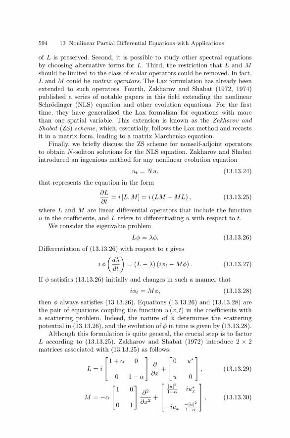
594 13 Nonlinear Partial Differential Equations with Applications
of L is preserved. Second, it is possible to study other spectral equationsby choosing alternative forms for L. Third, the restriction that L and Mshould be limited to the class of scalar operators could be removed. In fact,L and M could be matrix operators. The Lax formulation has already beenextended to such operators. Fourth, Zakharov and Shabat (1972, 1974)published a series of notable papers in this field extending the nonlinearSchrodinger (NLS) equation and other evolution equations. For the firsttime, they have generalized the Lax formalism for equations with morethan one spatial variable. This extension is known as the Zakharov andShabat (ZS) scheme, which, essentially, follows the Lax method and recastsit in a matrix form, leading to a matrix Marchenko equation.
Finally, we briefly discuss the ZS scheme for nonself-adjoint operatorsto obtain N -soliton solutions for the NLS equation. Zakharov and Shabatintroduced an ingenious method for any nonlinear evolution equation
ut = Nu, (13.13.24)
that represents the equation in the form
∂L
∂t= i [L, M ] = i (LM − ML) , (13.13.25)
where L and M are linear differential operators that include the functionu in the coefficients, and L refers to differentiating u with respect to t.
We consider the eigenvalue problem
Lφ = λφ. (13.13.26)
Differentiation of (13.13.26) with respect to t gives
i φ
(dλ
dt
)= (L − λ) (iφt − Mφ) . (13.13.27)
If φ satisfies (13.13.26) initially and changes in such a manner that
iφt = Mφ, (13.13.28)
then φ always satisfies (13.13.26). Equations (13.13.26) and (13.13.28) arethe pair of equations coupling the function u (x, t) in the coefficients witha scattering problem. Indeed, the nature of φ determines the scatteringpotential in (13.13.26), and the evolution of φ in time is given by (13.13.28).
Although this formulation is quite general, the crucial step is to factorL according to (13.13.25). Zakharov and Shabat (1972) introduce 2 × 2matrices associated with (13.13.25) as follows:
L = i
⎡⎣1 + α 0
0 1 − α
⎤⎦ ∂
∂x+
⎡⎣ 0 u∗
u 0
⎤⎦ , (13.13.29)
M = −α
⎡⎣1 0
0 1
⎤⎦ ∂2
∂x2 +
⎡⎢⎣|u|21+α iu∗
x
−iux−|u|21−α
⎤⎥⎦ , (13.13.30)

13.14 Exercises 595
and the NLS equation for complex u (x, t) is given by
iut + uxx + γ |u|2 u = 0, (13.13.31)
where
γ = 2/(1 − α2) .
Thus, the eigenvalue problem (13.13.26) and the evolution equation(13.13.28) complete the inverse scattering problem. The initial-value prob-lem for u (x, t) can be solved for a given initial condition u (x, 0). It seemsclear that the significant contribution would come from the point spectrumfor large times (t → ∞). Physically, the disturbance tends to disintegrateinto a series of solitary waves. The mathematical analysis is limited to theasymptotic solutions so that |u| → 0 as |x| → ∞, but a series of solitarywaves is expected to be the end result of the instability of wavetrains tomodulations.
13.14 Exercises
1. For the flow density relation q = vρ (1 − ρ/ρ1), find the solution of thetraffic flow problem with the initial condition ρ (x, 0) = f (x) for all x.Let
f (x) =
⎧⎪⎪⎪⎪⎨⎪⎪⎪⎪⎩
13 , x ≤ 0
13 + 5
12x, 0 ≤ x ≤ 1
34 , x ≥ 1.
Show that(i) ρ = 1
3ρ0 along the characteristic lines ct = 3 (x − x0), x0 ≤ 0,
(ii) ρ = 34ρ0 along the characteristic lines ct = 2 (x0 − x), x0 ≥ 1,
(iii) ρ = 13 + 5
12x0ρ0 along ct( 2
5 − x0)
= 65 (x − x0), 0 ≤ x0 ≤ 1.
Discuss what happens at the intersection of the two lines ct = 3x andct = 2 (1 − x). Draw the characteristic lines ct versus x.
2. A mountain of height h (x, t) is vulnerable to erosion if its slope hx isvery large. If ht and hx satisfy the functional relation ht = −Q (hx),show that u = hx is governed by the nonlinear wave equation
ut + c (u) ux = 0, c (u) = Q′ (u) .
3. Consider the flow of water in a river carrying some particles throughthe solid bed. During the sedimentation process, some particles will

596 13 Nonlinear Partial Differential Equations with Applications
be deposited in the bed. Assuming that v is the constant velocity ofwater and that ρ = ρf + ρb is the density, where ρf is the density ofthe particles carried in the fluid and ρb is the density of the materialdeposited on the solid bed, the conservation law is
∂ρ
∂t+
∂q
∂x= 0, q = vρf .
(a) Show that ρb satisfies the equation
∂ρf
∂t+ c (ρf )
∂ρf
∂x= 0, c (ρf ) =
v
1 + Q′ (ρf ),
where ρb = Q (ρf ) .
(b) This problem also arises in chemical engineering with a second re-lation between ρf and ρb in the form
∂ρb
∂t= k1 (α − ρb) − k2 (β − ρf ) ρb,
where k1, k2 represent constant reaction rates and α, β are constantvalues of the saturation levels of the particles in the solid bed and fluidrespectively. Show that the propagation speed c is
c =k2βv
(k1α + k2β)
provided that the densities are small.
4. Show that a steady solution u (x, t) = f (ζ), ζ = x − ct of Burgers’equation with the boundary conditions f → u−
∞ or u+∞ as ζ → −∞
or +∞ is
u (x, t) =[c − 1
2(u−
∞ − u+∞
)tanh
(u−
∞ − u+∞)
4ν(x − ct)
],
where u−∞ = c +
(c2 + 2A
) 12 , u+
∞ = c − (c2 − 2A
) 12 are two roots of
f2 − 2cf − 2A = 0 and A is a constant of integration.
5. Show that the transformations x → γ13 x, u → −6γ
13 u, t → t reduce
the KdV equation ut + uux + γuxxx = 0 into the canonical form ut −6uux + uxxx = 0.
Hence or otherwise, prove that the solution of the canonical equationwith the boundary conditions that u (x, t) and its derivatives tend tozero as |x| → ∞ is
u (x, t) = −a2
2sech2
a
2(x − a2t
).

13.14 Exercises 597
6. Verify that the Riccati transformation u = v2 + vx transforms the KdVequation so that v satisfies the associated KdV equation
vt − 6v2vx + vxxx = 0.
For a given u, show that the Riccati equation vx + v2 = u becomes thelinear Schrodinger equation, ψxx = uψ (without the energy-level term)under the transformation v = (ψx/ψ).
7. Apply the method of characteristics to solve the pair of equations
∂u
∂t+
∂v
∂x= 0,
∂v
∂t+
∂u
∂x= 0,
with the initial data
u (x, 0) = ex, v (x, 0) = e−x,
Show that the Riemann invariants are
2 r (α) = 2 cosh α, 2 s (β) = 2 sinhβ,
Also, show that solutions are u = cosh (x − t) + sinh (x + t) and v =cosh (x − t) − sinh (x + t).
8. For an isentropic flow, the Euler equations are
ρt + (ρu)x = 0,
ut + uux +1ρpx = 0,
St + uSx = 0,
where ρ is the density, u is the velocity in the x direction, p is thepressure, and S is the entropy.Show that this system has three families of characteristics.
Γ0 :dx
dt= u, Γ+ :
dx
dt= u + c,
where c2 =(
∂p∂ρ
)s
= constant.
Hence derive the following full set of characteristic equations
dS
dt= 0, on Γ0,
dp
dt+ ρc
du
dt= 0, on Γ+.
In particular, when the flow is isentropic (S = constant everywhere),show that the characteristic equations are∫
c (ρ)ρ
dρ + u = constant on Γ+ and Γ+ :dx
dt= u + c.

598 13 Nonlinear Partial Differential Equations with Applications
9. (a) Using equations (13.8.32)–(13.8.36), derive the second-order equa-tion
trs + φ (r + s) (tr + ts) = 0, φ (r + s) =12c
(1 +
ρ
c
dc
dρ
).
(b) For a polytropic gas, show that
φ (r + s) =γ + 1
4c=
α
F (ρ), α ≡ 1
2
(γ + 1γ − 1
),
and
trs +α
r + s(tr + ts) = 0.
(c) With F (ρ) = 2cγ−1 = r + s and u = r − s, show that the differential
equation in 9(b) reduces to the Euler–Poisson–Darboux equation
tuu −(
γ − 12
)2 (tcc +
2α
ctc
)= 0,
where u and c are independent variables.
10. Show that the KdV equation
ut − 6uux + uxxx = 0
satisfies the conservation law in the form Ut + Vx = 0 when (a) U = u,V = −3u2 + uxx, and (b) U = 1
2u2, V = −2u3 + uux − 12u2
x.
11. Show that the KdV equation
ut + 6uux + uxxx = 0
satisfies the conservation law
Ut + Vx = 0,
where(a) U = u, V = 3u2 + uxx,
(b) U = 12u2, V = 2u3 + uuxx − 1
2u2x,
(c) U = u3 − 12u2
x, V = 92 u4 + 3u2uxx + 1
2u2xx + uxut.
12. Show that the conservation laws for the associated KdV equation
vt − 6v2vx + vxxx = 0,
are
(a) (v)t +( 1
3 v3 + vxx
)x
= 0,
(b)( 1
2v2)t+
( 14 v4 + vvxx − 1
2v2x
)x
= 0.

13.14 Exercises 599
13. For the nonlinear Schrodinger equation (13.12.13), prove that∫ ∞
−∞T dx = constant,
where (i) T ≡ i(ψ ψx − ψ ψx
)and (ii) T ≡ |ψx|2 − 1
2γ |ψ|4.14. Show that the conservation law for Burgers’ equation (13.10.20) is
(u)t +(
12u2 + ν ux
)x
= 0.
15. Show that the conservation laws for the equation
ut − uux − uxxt = 0
are of the forms
(a) (u)t − ( 12u2 + uxt
)x
= 0,
(b) 12
(u2 + u2
x
)t− ( 1
3u3 + uuxt
)x
= 0.
16. Show that the linear Schrodinger system
i ψt + ψxx = 0, −∞ < x < ∞, t > 0,
ψ → 0, |x| → ∞,
ψ (x, 0) = ψ (x) with∫ ∞
−∞|ψ|2 dx = 1.
has the conservation law(i |ψ|2
)t+ (ψ∗ψx − ψψ∗
x)x = 0
and the energy integral ∫ ∞
−∞|ψ|2 dx = 1.
17. Seek a dispersive wave solution of the telegraph equation (see problem14, 3.9 Exercises)
utt − c2uxx + ac2ut + bc2u = 0
in the form
u (x, t) = A exp [i (kx − ωt)] .
(a) Show that ω = − 12
(iac2
)+ 1
2
[4c2k2 +
(4b − c2
)c2
] 12 .
(b) If 4b = a2c2, show that the solution
u (x, t) = A exp(
−12ac2t
)exp [ik (x+ ct)]
represents nondispersive waves with attenuation.

14
Numerical and Approximation Methods
“The strides that have been made recently, in the theory of nonlinear partialdifferential equations, are as great as in the linear theory. Unlike the linearcase, no wholesale liquidation of broad classes of problems has taken place;rather, it is steady progress on old fronts and on some new ones, the com-plete solution of some special problems, and the discovery of some brandnew phenomena. The old tools – variational methods, fixed point theorems,mapping degree, and other topological tools have been augmented by somenew ones. Pre-eminent for discovering new phenomena is numerical exper-imentation; but it is likely that in the future numerical calculations will beparts of proofs.”
Peter Lax
“Almost everyone using computers has experienced instances wherecomputational results have sparked new insights.”
Norman J. Zabusky
14.1 Introduction
The preceding chapters have been devoted to the analytical treatment oflinear and nonlinear partial differential equations. Several analytical meth-ods to find the exact analytical solution of these equations within simpledomains have been discussed. The boundary and initial conditions in theseproblems were also relatively simple, and were expressible in simple math-ematical form. In dealing with many equations arising from the modellingof physical problems, the determination of such exact solutions in a simpledomain is a formidable task even when the boundary and/or initial data aresimple. It is then necessary to resort to numerical or approximation meth-ods in order to deal with the problems that cannot be solved analytically. In
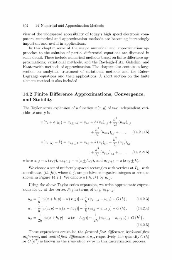
602 14 Numerical and Approximation Methods
view of the widespread accessibility of today’s high speed electronic com-puters, numerical and approximation methods are becoming increasinglyimportant and useful in applications.
In this chapter some of the major numerical and approximation ap-proaches to the solution of partial differential equations are discussed insome detail. These include numerical methods based on finite difference ap-proximations, variational methods, and the Rayleigh–Ritz, Galerkin, andKantorovich methods of approximation. The chapter also contains a largesection on analytical treatment of variational methods and the Euler–Lagrange equations and their applications. A short section on the finiteelement method is also included.
14.2 Finite Difference Approximations, Convergence,and Stability
The Taylor series expansion of a function u (x, y) of two independent vari-ables x and y is
u (xi + h, yj) = ui + 1,j = ui,j + h (ux)i,j +h2
2!(uxx)i,j
+h3
3!(uxxx)i,j + . . . , (14.2.1ab)
u (xi, yj + k) = ui,j + 1 = ui,j + k (uy)i,j +k2
2!(uyy)i,j
+k3
3!(uyyy)i,j + . . . , (14.2.2ab)
where ui,j = u (x, y), ui + 1,j = u (x+ h, y), and ui,j + 1 = u (x, y + k).
We choose a set of uniformly spaced rectangles with vertices at Pi,j withcoordinates (ih, jk), where i, j, are positive or negative integers or zero, asshown in Figure 14.2.1. We denote u (ih, jk) by ui,j .
Using the above Taylor series expansion, we write approximate expres-sions for ux at the vertex Pi,j in terms of ui,j , ui + 1,j :
ux =1h
[u (x + h, y) − u (x, y)] ∼ 1h
(ui+1,j − ui,j) + O (h) , (14.2.3)
ux =1h
[u (x, y) − u (x − h, y)] ∼ 1h
(ui,j − ui−1,j) + O (h) , (14.2.4)
ux =12h
[u (x + h, y) − u (x − h, y)] ∼ 12h
(ui+1,j − ui−1,j) + O(h2) .
(14.2.5)
These expressions are called the forward first difference, backward firstdifference, and central first difference of ux, respectively. The quantity O (h)or O
(h2
)is known as the truncation error in this discretization process.

14.2 Finite Difference Approximations, Convergence, and Stability 603
Figure 14.2.1 Uniformly spaced rectangles.
A similar approximate result for uxx at the vertex Pi,j is
uxx =1h2 [u (x + h, y) − 2 u (x, y) + u (x − h, y)]
∼ 1h2 [ui+1,j − 2 ui,j + ui−1,j ] + O
(h2) . (14.2.6)
Similarly, the approximate formulas for uy and uyy at Pi,j are
uy =1k
[u (x, y + k) − u (x, y)] ∼ 1k
(ui,j+1 − ui,j) + O (k) , (14.2.7)
uy =1k
[u (x, y) − u (x, y − k)] ∼ 1k
(ui,j − ui,j−1) + O (k) , (14.2.8)
uy =12k
[u (x, y + k) − u (x, y − k)] ∼ 12k
(ui,j+1 − ui,j−1) + O(k2) ,
(14.2.9)
uyy =1k2 [u (x, y + k) − 2 u (x, y) + u (x, y − k)]
∼ 1k2 [ui,j+1 − 2ui,j + ui,j−1] + O
(k2) . (14.2.10)
All these difference formulas are extremely useful in finding numericalsolutions of first or second order partial differential equations.
Suppose U (x, y) represents the exact solution of a partial differentialequation L (U) = 0 with independent variables x and y, and ui,j is theexact solution of the corresponding finite difference equation F (ui,j) = 0.Then, the finite difference scheme is said to be convergent if ui,j tends toU as h and k tend to zero. The difference, di,j ≡ (Ui,j − ui,j) is called thecummulative truncation (or discretization) error.
This error can generally be minimized by decreasing the grid sizes hand k. However, this error depends not only on h and k, but also on the

604 14 Numerical and Approximation Methods
number of terms in the truncated series which is used to approximate eachpartial derivative.
Another kind of error is introduced when a partial differential equationis approximated by a finite difference equation. If the exact finite differencesolution ui,j is replaced by the exact solution Ui,j of the partial differentialequation at the grid points Pi,j , then the value F (Ui,j) is called the localtruncation error at Pi,j . The finite difference scheme and the partial differ-ential equation are said to be consistent if F (Ui,j) tends to zero as h andk tend to zero.
In general, finite difference equations cannot be solved exactly becausethe numerical computation is carried out only up to a finite number ofdecimal places. Consequently, another kind of error is introduced in thefinite difference solution during the actual process of computation. Thiskind of error is called the round-off error, and it also depends upon thetype of computer used. In practice, the actual computational solution isu∗
i,j , but not ui,j , so that the difference ri,j =(ui,j − u∗
i,j
)is the round-
off error at the grid point Pi,j . In fact, this error is introduced into thesolution of the finite difference equation by round-off errors. In reality, theround-off error depends mainly on the actual computational process andthe finite difference itself. In contrast to the cummulative truncation error,the round-off error cannot be made small by allowing h and k to tend tozero.
Thus, the total error involved in the finite difference analysis at thepoint Pi,j is given by(
Ui,j − u∗i,j
)= (Ui,j − ui,j) +
(ui,j − u∗
i,j
)= di,j − ri,j . (14.2.11)
Usually the discretization error di,j is bounded when ui,j is boundedbecause the value of Ui,j is fixed for a given partial differential equationwith the prescribed boundary and initial data. This fact is used or assumedin order to introduce the concept of stability. The finite difference algo-rithm is said to be stable if the round-off errors are sufficiently small forall i as j → ∞, that is, the growth of ri,j can be controlled. It should bepointed out again that the round-off error depends not only on the actualcomputational process and the type of computer used, but also on the finitedifference equation itself. Lax (1954) proved a remarkable theorem whichestablishes the relationship between consistency, stability, and convergencefor the finite difference algorithm.
Theorem 14.2.1. (Lax’s Equivalence Theorem). Given a properly posedlinear initial-value problem and a finite difference approximation to it thatsatisfies the consistency criterion, stability is a necessary and sufficientcondition for convergence.

14.3 Lax–Wendroff Explicit Method 605
Von Neumann’s Stability Method
This method is essentially based upon a finite Fourier series. It expressesthe initial errors on the line t = 0 in terms of a finite Fourier series and thenexamines the propagation of errors as t → ∞. It is convenient to denotethe error function by er,s instead of ei,j so that er,s gives the initial valueser,0 = e (rh) = er on the line t = 0 between x = 0 and x = l, where r = 0,1, 2, . . ., N and Nh = l. The finite Fourier series expansion of er is
er =N∑
n=0
An exp (inπx/l) =N∑
n=0
An exp (iαnrh) , (14.2.12)
where αn = (nπ/l), x = rh, and An are the Fourier coefficients which aredetermined from the (N + 1) equations (14.2.12).
Since we are concerned with the linear finite difference scheme, errorsform an additive system so that the total error can be found by the superpo-sition principle. Thus, it is sufficient to consider a single term exp (iαrh) inthe Fourier series (14.2.12). Following the method of separation of variablescommonly used for finding the analytical solution of a partial differentialequation, we seek a separable solution of the finite difference equation forer,s in the form
er,s = exp (iαrh + βsk) = exp (iαrh) ps (14.2.13)
which reduces to exp (iαrh) at s = 0 (t = sk = 0), where p = exp (βk), andβ is a complex constant. This shows that the error is bounded as (t → ∞)provided that
|p| ≤ 1 (14.2.14)
is satisfied. This condition is found to be necessary and sufficient for thestability of the finite difference algorithm.
14.3 Lax–Wendroff Explicit Method
To describe this method, we consider the first-order conservation equation
∂u
∂t+ c
∂u
∂x= 0 (14.3.1)
where u ≡ u (x, t) is some physical function of space variable x and time t.This equation occurs frequently in applied mathematics.
Lax and Wendroff use the Taylor series expansion in t in the form
ui,j+1 = ui,j + k (ut)i,j +k2
2!(utt)i,j +
k3
3!(uttt)i,j + . . . , (14.3.2)

606 14 Numerical and Approximation Methods
where k ≡ δt.The partial derivatives in t in (14.3.2) can easily be eliminated by using
ut = −c ux so that (14.3.2) becomes
ui,j+1 = ui,j − c k (ux)i,j +c2k2
2(uxx)i,j − . . . . (14.3.3)
Replacing ux, uxx by the central difference formulas, (14.3.3) becomes
ui,j+1 = ui,j −(
ck
2h
)(ui+1,j − ui−1,j) +
12
(ck
h
)2
(ui+1,j − 2 ui,j + ui−1,j) ,
or
ui,j+1 =(1 − ε2)ui,j +
ε
2(1 + ε) ui−1,j − ε
2(1 + ε) ui+1,j + O
(ε3) ,(14.3.4)
where ε = (ck/h). This is called the Lax–Wendroff second-order finite dif-ference scheme; it has been widely used to solve first-order hyperbolic equa-tions.
Von Neumann criterion (14.2.14) can be applied to investigate the sta-bility of the Lax–Wendroff scheme. It is noted that the error function er,s
given by (14.2.13) satisfies the finite difference equation (14.3.4). We thensubstitute (14.2.13) into (14.3.4) and cancel common factors to obtain
p =(1 − ε2) +
ε
2[(1 + ε) e−iαh − (1 − ε) eiαh
]= 1 − 2 ε2 sin2
(αh
2
)− 2iε sin
(αh
2
)cos
(αh
2
),
so that
|p|2 = 1 − 4ε2 (1 − ε2) sin4
(αh
2
). (14.3.5)
According to the von Neumann criterion, the Lax–Wendroff scheme(14.3.4) is stable as t → ∞ if |p| ≤ 1, which gives 4ε2
(1 − ε2
) ≥ 0, that is,0 < ε ≤ 1.
The local truncation error of the Lax–Wendroff equation (14.3.4) at Pi,j
is
Ti,j =1k
(ui,j+1 − ui−1,j)
which is, by (14.2.2a) and (14.2.1b) with ck = h (ε = 1),
= (ut + cux)i,j +k
2(utt − c2uxxx
)i,j
+k2
6(uttt + c3uxxx
)i,j
+ O((ck)3
).
(14.3.6)

14.3 Lax–Wendroff Explicit Method 607
The first two terms on the right side of (14.3.6) vanish by equation (14.3.1)so that the local truncation error becomes
Ti,j =16(k2uttt + c h2uxxx
)i,j
. (14.3.7)
Another approximation to (14.3.1) with first-order accuracy is
1k
(ui,j+1 − ui,j) +c
h(ui,j − ui−1,j) = 0. (14.3.8)
A final explicit scheme for (14.3.1) is based on the central difference ap-proximation. This scheme is called the leap frog algorithm. In this method,the finite difference approximation to (14.3.1) is
12k
(ui,j+1 − ui,j−1) +c
2h(ui+1,j − ui−1,j) = 0,
or,
ui,j+1 = ui,j−1 − ε (ui+1,j − ui−1,j) . (14.3.9)
As shown in Figure 14.3.1, this equation shows that the value of u atPi,j+1 is computed from the previously computed values at three grid pointsat two previous time steps.
Figure 14.3.1 Grid system for the leap frog algorithm.

608 14 Numerical and Approximation Methods
14.4 Explicit Finite Difference Methods
(A) Wave Equation and the Courant–Friedrichs–LewyConvergence Criterion
The method of characteristics provides the most convenient and accurateprocedure for solving Cauchy problems involving hyperbolic equations. Oneof the main advantages of this method is that discontinuities of the initialdata propagate into the solution domain along the characteristics. However,when the initial data are discontinuous, the finite difference algorithm forthe hyperbolic systems is not very convenient. Problems concerning hyper-bolic equations with continuous initial data can be solved successfully byfinite difference methods with rectangular grid systems.
A commonly cited problem is the propagation of a one-dimensional wavegoverned by the system
utt = c2 uxx, −∞ < x < ∞, t > 0, (14.4.1)u (x, 0) = f (x) , ut (x, 0) = g (x) for all x ∈ R. (14.4.2)
Using a rectangular grid system with h = δx, k = δt, ui,j = u (ih, jk),−∞ < x < ∞, and 0 ≤ j < ∞, the central difference approximation toequation (14.4.1) is
1k2 (ui,j+1 − 2 ui,j + ui,j−1) =
c2
h2 (ui+1,j − 2 ui,j + ui−1,j) ,
or,
ui,j+1 = ε2 (ui+1,j + ui−1,j) + 2(1 − ε2)ui,j − ui,j−1, (14.4.3)
where ε ≡ (ck/h), and is often called the Courant parameter. This explicitformula allows us to determine the approximate values at the grid pointson the lines t = 2k, 3k, 4k, . . ., when the grid values at t = k have beenobtained.
The approximate values of the initial data on the line t = 0 are
ui,0 = fi,12k
(ui,1 − ui,−1) = gi,0 (14.4.4)
so that the second result gives
ui,−1 = ui,1 − 2k gi,0. (14.4.5)
When j = 0 in (14.4.3) and (14.4.5) is used, we obtain
ui,1 =12
ε2 (fi−1 + fi+1) +(1 − ε2) fi + k gi,0. (14.4.6)
This result determines grid values on the line t = k.

14.4 Explicit Finite Difference Methods 609
Figure 14.4.1 Computational grid systems and characteristics.
The value of u at Pi,j+1 is obtained in terms of its previously calculatedvalues at Pi + 1,j , Pi,j , and Pi,j−1, which are determined from previouslycomputed values on the lines t = (j − 1) k, (j − 2) k, (j − 3) k. Thus, thecomputation from the lines t = 0 and t = k suggests that u at Pi,j will rep-resent a function of the values of u within the domain bounded by the linesdrawn back toward t = 0 from P whose gradients are (+ ε) as shown in Fig-ure 14.4.1. Thus the triangular regions PAB, PCD represent the domainsof dependence at P of the solutions of the finite difference equation (14.4.3)and the differential equation (14.4.1). By analogy with real characteristiclines PC and PD of the differential equation, the straight lines PA andPB are called the numerical characteristics. Thus, it follows from Figure14.4.1 that ∆PAB lies inside ∆PCD, which means that the solution of thefinite difference system at P would remain unchanged even when the initialdata along PA and PB are changed. Courant, Friedrichs and Lewy (CFL,1928) proved that the solution of the finite difference system converges tothat of the differential equation system as h and k tend to zero providedthat the domain of dependence of the difference equation lies inside that ofthe partial differential equation. This condition for convergence is knownas the CFL condition, which means 1/c ≥ k/h, that is, 0 < ε ≤ 1.
If the Courant parameter is ε = 1, equation (14.4.3) reduces to a simpleform

610 14 Numerical and Approximation Methods
ui,j+1 = ui+1,j + ui−1,j − ui,j−1. (14.4.7)
As shown in Figure 14.3.1, this equation shows that the value of u atPi,j+1 is computed from the previously computed values at three grid pointsat two previous time steps. This is called the leap frog algorithm.
From equation (5.3.4) in Chapter 5, we know that the solution of theCauchy problem for the wave equation has the form
u (x, t) = φ (x + ct) + ψ (x − ct) ,
where the functions φ and ψ represent waves propagating without changingshape along the negative and positive x directions with a constant speedc. The lines of slope (dt/dx) = + (1/c) in the x − t plane, which trace theprogress of the waves, are known as the characteristics of the wave equation.
In terms of a grid point (xi, tj), the above solution has the form
ui,j = φ (xi + c tj) + ψ (xi − c tj) . (14.4.8)
It follows from Figure 14.3.1 that xi = x1 + (i − 1) h and tj = t1 +(j − 1) k so that (14.4.8) takes the form
ui,j = φ (α + ih + jck) + ψ (β + ih − jck) , (14.4.9)
where
α = (x1 − h) + c (t1 − k) , β = (x1 − h) − c (t1 − k) .
Since ε = 1, ck = h, solution (14.4.9) becomes
ui,j = φ (α + (i + j) h) + ψ (β + (i − j) h) .
This satisfies equation (14.4.7). It follows that the leap frog methodgives the exact solution of the partial differential equation (14.4.1).
We apply von Neumann stability analysis to investigate the stability ofthe above numerical method for the wave equation. We seek a separablesolution of the error function er,s as
er,s = exp (iαrh) ps, (14.4.10)
where p = exp (βk). This function satisfies the finite difference equation(14.4.3). Substituting (14.4.10) into (14.4.3) and cancelling the commonfactors, we obtain the quadratic equation for p
p2 − 2 b p + 1 = 0, (14.4.11)
where b = 1 − 2ε2 sin2 (αh/2), ε = (ck/h), and b ≤ 1 for all real ε and α.This quadratic equation has two complex roots p1 and p2 if b2 < 1. Sincep1 ·p2 = 1, it follows that one of the roots will always have modulus greater
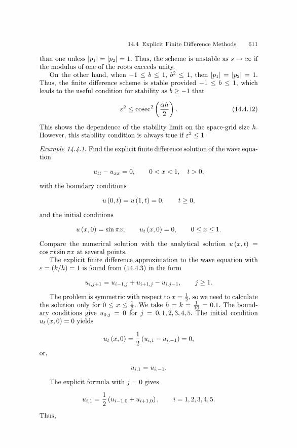
14.4 Explicit Finite Difference Methods 611
than one unless |p1| = |p2| = 1. Thus, the scheme is unstable as s → ∞ ifthe modulus of one of the roots exceeds unity.
On the other hand, when −1 ≤ b ≤ 1, b2 ≤ 1, then |p1| = |p2| = 1.Thus, the finite difference scheme is stable provided −1 ≤ b ≤ 1, whichleads to the useful condition for stability as b ≥ −1 that
ε2 ≤ cosec2(
αh
2
). (14.4.12)
This shows the dependence of the stability limit on the space-grid size h.However, this stability condition is always true if ε2 ≤ 1.
Example 14.4.1. Find the explicit finite difference solution of the wave equa-tion
utt − uxx = 0, 0 < x < 1, t > 0,
with the boundary conditions
u (0, t) = u (1, t) = 0, t ≥ 0,
and the initial conditions
u (x, 0) = sinπx, ut (x, 0) = 0, 0 ≤ x ≤ 1.
Compare the numerical solution with the analytical solution u (x, t) =cos πt sin πx at several points.
The explicit finite difference approximation to the wave equation withε = (k/h) = 1 is found from (14.4.3) in the form
ui,j+1 = ui−1,j + ui+1,j − ui,j−1, j ≥ 1.
The problem is symmetric with respect to x = 12 , so we need to calculate
the solution only for 0 ≤ x ≤ 12 . We take h = k = 1
10 = 0.1. The bound-ary conditions give u0,j = 0 for j = 0, 1, 2, 3, 4, 5. The initial conditionut (x, 0) = 0 yields
ut (x, 0) =12
(ui,1 − ui,−1) = 0,
or,
ui,1 = ui,−1.
The explicit formula with j = 0 gives
ui,1 =12
(ui−1,0 + ui+1,0) , i = 1, 2, 3, 4, 5.
Thus,

612 14 Numerical and Approximation Methods
u1,1 =12
(u0,0 + u2,0) =12u2,0 =
12
sin (0.2π) = 0.2939.
Similarly,
u2,1 = 0.5590, u3,1 = 0.7695, u4,1 = 0.9045, u5,1 = 0.9511.
We next use the basic explicit formula to compute
u1,2 = u0,1 + u2,1 − u1,0 = 0 + 0.5590 − 0.3090 = 0.2500,
u2,2 = u1,1 + u3,1 − u2,0 = 0.2939 + 0.7695 − 0.5878 = 0.4756.
Similarly, we compute other values for ui,j which are shown in Table 14.4.1.The analytical solutions at (x, t) = (0.1, 0.1) and (0.2, 0.3) are given by
u (0.1, 0.1) = cos (0.1π) sin (0.1π) = (0.9511) (0.3090) = 0.2939,
u (0.2, 0.2) = cos (0.2π) sin (0.2π) = (0.8090) (0.5878) = 0.4577,
u (0.2, 0.3) = cos (0.3π) sin (0.2π) = (0.5878) (0.5878) = 0.3455.
Comparison of the analytical solutions with the above finite differencesolutions shows that the latter results are very accurate.
(B) Parabolic Equations
As a prototype diffusion problem, we consider
ut = κuxx, 0 < x < 1, t > 0, (14.4.13)u (0, t) = u (1, t) = 0, for all t, (14.4.14)u (x, 0) = f (x) , for all x in (0, 1) , (14.4.15)
where f (x) is a given function.
Table 14.4.1.
i 0 1 2 3 4 5x 0.0 0.1 0.2 0.3 0.4 0.5
j t
1 0.1 0 0.2939 0.5590 0.7695 0.9045 0.95112 0.2 0 0.2500 0.4577 0.6545 0.7695 0.80903 0.3 0 0.1817 0.3455 0.4756 0.5590 0.58784 0.4 0 0.9045 0.7695 0.2500 0.2939 0.30905 0.5 0 0 0 0 0 0

14.4 Explicit Finite Difference Methods 613
The explicit finite difference approximation to (14.4.13) is
1k
(ui,j+1 − ui,j) =κ
h2 (ui+1,j − 2 ui,j + ui−1,j) , (14.4.16)
or,
ui,j+1 = ε (ui+1,j + ui−1,j) + (1 − 2 ε) ui,j , (14.4.17)
where ε =(κk/h2
).
This explicit finite difference formula gives approximate values of u ont = (j + 1) k in terms of values on t = jk with given ui,0 = fi. Thus, ui,j
can be obtained for all j by successive use of (14.4.17).The problems of stability and convergence of the parabolic equation are
similar to those of the wave equation. It can be shown that the solution ofthe finite difference equation converges to that of the differential equationsystem (14.4.13)–(14.4.15) as h and k tend to zero provided ε ≤ 1
2 .In particular, when ε = 1
2 , equation (14.4.17) takes a simple form
ui,j+1 =12
(ui+1,j + ui−1,j) . (14.4.18)
This is called the Bender–Schmidt explicit formula which determines thesolution at (xi, tj+1) as the mean of the values at the grid points (i+ 1, j).However, more accurate results can be found from (14.4.17) for ε < 1
2 .To investigate the stability of the numerical scheme, we assume that the
error function is
er,s = exp (iαrh) ps, (14.4.19)
where p = eβk. The error function and urs satisfy the same differenceequation. Hence, we substitute (14.4.19) into (14.4.17) to obtain
p = 1 − 4 ε sin2(
αh
2
). (14.4.20)
Clearly, p is always less than 1 because ε > 0. If p ≥ 0, the function givenby (14.4.19) will decay steadily as s = j → ∞. If −1 < p < 0, then thesolution will have a decaying amplitude as s → ∞. Therefore, the finitedifference scheme will be stable if p > −1, that is, if
0 < ε ≤ 12
cosec2(
αh
2
). (14.4.21)
This shows that the stability limit depends on h. However, in view of theinequality
ε ≤ 12
≤ 12
cosec2(
αh
2
),
we conclude that the stability condition is ε ≤ 12 . Finally, if p < −1, the
solution oscillates with increasing amplitude as s → ∞, and hence, thescheme will be unstable for ε > 1
2 .

614 14 Numerical and Approximation Methods
Example 14.4.2. Show that the Richardson explicit finite difference schemefor (14.4.13) is unconditionally unstable.
The Richardson finite difference approximation to (14.4.13) is
12k
(ui,j+1 − ui,j−1) =κ
h2 (ui+1,j − 2 ui,j + ui−1,j) . (14.4.22)
To establish the instability of this equation, we use the Fourier methodand assume that
er,s = exp (iαrh) ps, p = eβk.
This function satisfies the Richardson difference equation as does ur,s. Con-sequently,
p − 1p
= −8 ε sin2(
αh
2
),
or
p2 + 8 p ε sin2(
αh
2
)− 1 = 0.
This quadratic equation has two roots
p1, p2 = −4 ε sin2(
αh
2
)+
(1 + 16 ε2 sin4 αh
2
) 12
, (14.4.23)
or
p1, p2 = + 1 − 4 ε sin2(
αh
2
)(1 + 2 ε sin2 αh
2
)+ O
(ε4) .
This gives |p1| ≤ 1 and
|p2| > 1 + 4 ε sin2(
αh
2
)> 1
for all positive ε and, consequently, the Richardson scheme is always un-stable.
The unstable feature of the Richardson scheme can be eliminated byreplacing ui,j with 1
2 (ui,j+1 + ui,j−1) in (14.4.22), which now becomes
(1 + 2 ε) ui,j+1 = 2 ε (ui+1,j + ui−1,j) + (1 − 2 ε) ui,j−1. (14.4.24)
This is called the Du Fort–Frankel explicit algorithm, and it can beshown to be stable for all ε.

14.4 Explicit Finite Difference Methods 615
Example 14.4.3. Prove that the solution of the finite difference equation forthe diffusion equation (14.4.13) in −∞ < x < ∞ with the initial conditionu (x, 0) = eiαx converges to the exact solution of (14.4.13) as h and k tendto zero.
We obtain the exact solution of (14.4.13) by seeking a separable form
u (x, t) = eiαx v (t) ,
where v (t) is a function of t alone which is to be determined.Substituting this solution into (14.4.13) gives
dv
dt+ κα2 v = 0
which admits solutions
v (t) = A e−κα2t,
where A is an integrating constant. The initial condition v (0) = 1 givesA = 1. Hence,
u (x, t) = exp(iαx − α2κt
). (14.4.25)
We now solve the corresponding finite difference equation (14.4.17) byreplacing i, j with r, s. We seek a separable solution of the differenceequation
ur,s = eiαrh vs
with the initial condition
ur,0 = eiαrh v0, so that v0 = 1.
Substituting this solution into the finite difference equation (14.4.7)yields
vs+1 =(
1 − 4 ε sin2 αh
2
)vs, v0 = 1,
so that the solution can be obtained by a simple inspection as
vs =(
1 − 4 ε sin2 αh
2
)s
, (14.4.26)
ur,s = eiαrh
(1 − 4ε sin2 αh
2
)s
, (14.4.27)
where ε =(κk/h2
).
For small h, 1 − 4 ε sin2 (αh/2) ∼ 1 − ε α2h2 so that 1 − ε α2h2 ≈exp
(−ε α2h2)
for small ε α2h2 = κα2k. Consequently, the final solutionbecomes

616 14 Numerical and Approximation Methods
ur,s ∼ eiαrh−κα2ks as h, k → 0. (14.4.28)
This is identical with the exact solution of the differential equation (14.4.13)with rh = x and sk = t. This example shows that the finite differenceapproximation is reasonably good.
Example 14.4.4. Calculate a finite difference solution of the initial boundary-value problem
ut = uxx, 0 < x < 1, t > 0,
with the boundary conditions
u (0, t) = u (1, t) = 0, t ≥ 0,
and the initial condition
u (x, 0) = x (1 − x) , 0 ≤ x ≤ 1.
Compare the numerical solution with the exact analytical solution atx = 0.04 and t = 0.02.
The explicit finite difference approximation to the parabolic equation is
ui,j+1 = ε ui−1,j + (1 − 2 ε) ui,j + ε ui+1,j ,
where ε =(k/h2
). This gives the unknown value ui,j+1 at the (i, j + 1) th
grid point in terms of given values of u along the jth time row.
We set h = 15 and k = 1
100 so that ε =(k/h2
)= 1
4 and the aboveformula becomes
ui,j+1 =14
(ui−1,j + 2 ui,j + ui+1,j) .
With the notation ui,0 = u (ih, 0), the initial condition gives
u4,0 = 0.16, and u5,0 = 0.
The boundary conditions yield u0,j = u (0, jk) = 0 and u5,j =u (5h, jk) = u (1, jk) = 0, for all j = 0, 1, 2, . . ..
Using these initial and boundary data, we calculate ui,j as follows:
u1,1 =14
(u0,0 + 2u1,0 + u2,0) = 0.14, u1,2 =14
(u0,1 + 2u1,1 + u2,1)
= 0.125,
u2,1 =14
(u1,0 + 2u2,0 + u3,0) = 0.22, u2,2 =14
(u1,1 + 2u2,1 + u3,1)
= 0.200,
u3,1 =14
(u2,0 + 2u3,0 + u4,0) = 0.22, u3,2 =14
(u2,1 + 2u3,1 + u4,1)
= 0.200,
u4,1 =14
(u3,0 + 2u4,0 + u5,0) = 0.14, u4,2 =14
(u3,1 + 2u4,1 + u5,1)
= 0.125,
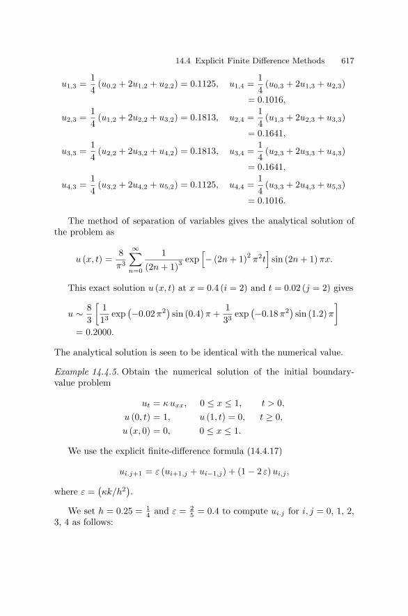
14.4 Explicit Finite Difference Methods 617
u1,3 =14
(u0,2 + 2u1,2 + u2,2) = 0.1125, u1,4 =14
(u0,3 + 2u1,3 + u2,3)
= 0.1016,
u2,3 =14
(u1,2 + 2u2,2 + u3,2) = 0.1813, u2,4 =14
(u1,3 + 2u2,3 + u3,3)
= 0.1641,
u3,3 =14
(u2,2 + 2u3,2 + u4,2) = 0.1813, u3,4 =14
(u2,3 + 2u3,3 + u4,3)
= 0.1641,
u4,3 =14
(u3,2 + 2u4,2 + u5,2) = 0.1125, u4,4 =14
(u3,3 + 2u4,3 + u5,3)
= 0.1016.
The method of separation of variables gives the analytical solution ofthe problem as
u (x, t) =8π3
∞∑n=0
1(2n + 1)3
exp[− (2n + 1)2 π2t
]sin (2n + 1)πx.
This exact solution u (x, t) at x = 0.4 (i = 2) and t = 0.02 (j = 2) gives
u ∼ 83
[113 exp
(−0.02 π2) sin (0.4) π +133 exp
(−0.18 π2) sin (1.2) π
]= 0.2000.
The analytical solution is seen to be identical with the numerical value.
Example 14.4.5. Obtain the numerical solution of the initial boundary-value problem
ut = κuxx, 0 ≤ x ≤ 1, t > 0,
u (0, t) = 1, u (1, t) = 0, t ≥ 0,
u (x, 0) = 0, 0 ≤ x ≤ 1.
We use the explicit finite-difference formula (14.4.17)
ui.j+1 = ε (ui+1,j + ui−1,j) + (1 − 2 ε) ui,j ,
where ε =(κk/h2
).
We set h = 0.25 = 14 and ε = 2
5 = 0.4 to compute ui.j for i, j = 0, 1, 2,3, 4 as follows:

618 14 Numerical and Approximation Methods
i 0 1 2 3 4j
0 1.000 0.000 0.000 0.000 0.0001 1.000 0.400 0.000 0.000 0.0002 1.000 0.480 0.160 0.000 0.0003 1.000 0.560 0.224 0.064 0.0004 1.000 0.602 0.295 0.103 0.000
(C) Elliptic Equations
As a prototype boundary-value problem, we consider the Dirichlet problemfor the Laplace equation
∇2u ≡ uxx + uyy = 0, 0 ≤ x ≤ a, 0 ≤ y ≤ b, (14.4.29)
where the value of u (x, y) is prescribed everywhere on the boundary of therectangular domain.
The rectangular grid system is the most common and convenient systemfor this problem. We choose the vertices of the rectangular domain as thenodal points and set h = a/m and k = b/n where m and n are positiveintegers so that the domain is divided into mn subrectangles.
The finite difference approximation to the Laplace equation (14.4.29) is
1h2 (ui+1,j − 2ui,j + ui−1,j) +
1k2 (ui,j+1 − 2ui,j + ui,j−1) = 0,(14.4.30)
or,
2(h2 + k2)ui,j = k2 (ui+1,j + ui−1,j) + h2 (ui,j+1 + ui,j−1) , (14.4.31)
where 1 ≤ i ≤ m − 1 and 1 ≤ j ≤ n − 1.The prescribed conditions on the boundary of the rectangular domain
determine the values u0,j , um,j , ui,0, and ui,n. For a square grid system(k = h), equation (14.4.30) becomes
ui,j =14
(ui+1,j + ui−1,j + ui,j+1 + ui,j−1) . (14.4.32)
This means that the value of u at an interior point is equal to the averageof the value of u at four adjacent points. This is the well known mean valuetheorem for harmonic functions that satisfy the Laplace equation.
As i and j vary, the present scheme reduces to a set of (m − 1) (n − 1)linear non-homogeneous algebraic equations for (m − 1) (n − 1) unknownvalues of u at interior grid points. It can be shown the solution of the finite

14.4 Explicit Finite Difference Methods 619
difference equation (14.4.31) converges to the exact solution of the problemas h, k → 0. The proof of the existence of a solution and its convergenceto the exact solution as h and k tend to zero is essentially based on theMaximum Modulus Principle. It follows from the finite difference equation(14.4.30) or (14.4.31) that the value of |u| at any interior grid point doesnot exceed its value at any of the four adjoining nodal points. In otherwords, the value of u at Pi,j cannot exceed its values at the four adjoiningpoints Pi + 1,j and Pi,j + 1. The successive application of this argument atall interior grid points leads to the conclusion that |u| at the interior gridpoints cannot be greater than the maximum value of |u| on the boundary.This may be recognized as the finite difference analogue of the MaximumModulus Principle discussed in Section 9.2. Thus, the success of the nu-merical method is directly associated with the existence of the MaximumModulus Principle.
Clearly, the present numerical algorithm deals with a large number ofalgebraic equations. Even though numerical accuracy can be improved bymaking h and k sufficiently small, there is a major computational difficultyinvolved in the numerical solution of a large number of equations. It ispossible to handle such a large number of algebraic equations by directmethods or by iterative methods, but it would be very difficult to obtaina numerical solution with sufficient accuracy. It is therefore necessary todevelop some alternative methods of solution that can be conveniently andefficiently carried out on a computer.
In order to eliminate some of the drawbacks stated above, one of the nu-merical schemes, the Liebmann’s iterative method, is useful. In this methodvalues of u are first guessed for all interior grid points in addition to thosegiven as the boundary points on the edges of the given domain. These valuesare denoted by u
(0)i,j where the superscript 0 indicates the zeroth iteration.
It is convenient to choose a square grid so that the simplified finite differ-ence equation (14.4.32) can be used. The values of u are calculated for thenext iteration by using (14.4.32) at every interior point based on the valuesof u at the present iteration. The sequence of computation starts from theinterior grid point located at the lowest left corner, proceeds upward un-til reaching the top, and then goes to the bottom of the next vertical lineon the right. This process is repeated until the new value of u at the lastinterior grid point at the upper right corner has been obtained.
At the starting point, formula (14.4.32) gives
u(1)2,2 =
14
(u
(0)3,2 + u
(0)1,2 + u
(0)2,3 + u
(0)2,1
), (14.4.33)
where u(0)1,2 and u
(0)2,1 are boundary values which remain constant during
the iteration process. They may be replaced, respectively, with u(1)1,2, u
(1)2,1 in
(14.4.33). The computation at the next step involves u(0)2,2. Since an improved
value u(1)2,2 is available at this time, it will be utilized instead. Hence,

620 14 Numerical and Approximation Methods
u(1)2,3 =
14
(u
(0)3,3 + u
(1)1,3 + u
(0)2,4 + u
(1)2,2
), (14.4.34)
where u(1)1,3 is used to replace the constant boundary value u
(0)1,3.
We repeat this argument to obtain a general iteration formula for com-putation of u at step (n + 1)
u(n+1)i,j =
14
(u
(n)i+1,j + u
(n+1)i−1,j + u
(n)i,j+1 + u
(n+1)i,j−1
). (14.4.35)
This result is valid for any interior point, whether it is next to some bound-ary point or not. If Pi,j is a true point, the second and fourth terms on theright side of (14.4.35) represent, respectively, the values of u at the gridpoints to the left of and below that point. These values have already beenrecomputed according to our scheme, and therefore, carry the superscript(n + 1). Result (14.4.35) is known as the Liebmann (n + 1) th iteration for-mula. It can be proved that u
(n)i,j converges to ui,j as n → ∞.
Another iteration scheme similar to (14.4.35) is given by
u(n+1)i,j =
14
(u
(n)i+1,j + u
(n)i−1,j + u
(n)i,j+1 + u
(n)i,j−1
). (14.4.36)
This is called the Richardson iteration formula, and it is also useful. How-ever, this scheme converges more slowly than that based on (14.4.35).
One of the major difficulties of the above methods is the slow rate of con-vergence. An improved numerical method, the Successive Over-Relaxation(SOR) scheme gives a faster convergence than the Liebmann or Richardsonmethod in solving the Laplace (or the Poisson) equation. For a rectangulardomain of square grids, the successive iteration scheme is given by
u(n+1)i,j = u
(n)i,j +
ω
4
(u
(n+1)i−1,j + u
(n)i+1,j + u
(n+1)i,j−1 + u
(n)i,j+1 − 4 u
(n)i,j
), (14.4.37)
where ω is called the acceleration parameter (or relaxation factor) to bedetermined. In general, ω lies in the range 1 ≤ ω < 2. The successiveiterations converge fairly rapidly to the desired solution for 1 ≤ ω < 2. Themost rapid rate of convergence is achieved for the optimum value of ω.
Example 14.4.6. Obtain the standard five-point formula for the Poissonequation
uxx + uyy = −f (x, y) in D ⊂ R2
with the prescribed value of u (x, y) on the boundary ∂D.We assume that the domain D is covered by a system of squares with
sides of length h parallel to the x and y axes. Using the central differenceapproximation to the Laplace operator, we obtain
1h2 (ui+1,j − 2 ui,j + ui−1,j) +
1h2 (ui,j+1 − 2 ui,j + ui,j−1) = −fi,j ,

14.4 Explicit Finite Difference Methods 621
or,
ui,j =14
(ui+1,j + ui−1,j + ui,j+1 + ui,j−1) +14
h2fi,j
where fi,j = f (ih, jh). This is known as the five-point formula.
Example 14.4.7. Find the numerical solution of the torsion problem in asquare beam governed by
∇2u = −2 in D = (x, y) : 0 ≤ x ≤ 1, 0 ≤ y ≤ 1with u (x, y) = 0 on ∂D.
From the above five-point formula, we obtain
ui,j =14
(ui+1,j + ui−1,j + ui,j+1 + ui,j−1) − 12h2
where h is the side-length of the unit square net.We choose h = 1
2 , 1/22, 1/23, 1/24 to calculate the corresponding nu-merical values ui,j = 0.1250, 0.1401, 0.1456, 0.1469.
Note that the known exact analytical solution is 0.1474.
Example 14.4.8. Using the explicit finite difference method, find the solu-tion of the Dirichlet problem
uxx + uyy = 0, in 0 < x < 1, 0 < y < 1,
u (x, 0) = x, u (x, 1) = 0, on 0 ≤ x ≤ 1,
u (x, y) = 0, for x = 0, x = 1 and 0 ≤ y ≤ 1.
We use four interior grid points (that is, i, j = 1, 2, 3, 4) as shown inFigure 14.4.2 in the (x, y)-plane.
We apply the explicit finite difference formula (14.4.32) to obtain fouralgebraic equations
−4u2,2 + u3,2 + u1,2 + u2,3 + u2,1 = 0,
−4u2,3 + u3,3 + u1,3 + u2,4 + u2,2 = 0,
−4u3,2 + u4,2 + u2,2 + u3,3 + u3,1 = 0,
−4u3,3 + u4,3 + u2,3 + u3,4 + u3,2 = 0.
The given boundary conditions imply that u2,1 = u2,4 = u3,1 = u3,4 =u4,2 = u4,3 = 0, u1,2 = 1
3 and u1,3 = 23 so that the above system of equations
becomes
−4u2,2 + u3,2 +13
+ u2,3 = 0,
−4u2,3 + u3,3 +23
+ u2,2 = 0,
−4u3,2 + u2,2 + u3,3 = 0,
−4u3,3 + u2,3 + u3,2 = 0.

622 14 Numerical and Approximation Methods
Figure 14.4.2 The square grid system.
In matrix notation, this system reads as⎡⎢⎢⎢⎢⎢⎢⎢⎢⎣
−4 1 1 0
1 −4 0 1
1 0 −4 1
0 1 1 −4
⎤⎥⎥⎥⎥⎥⎥⎥⎥⎦
⎡⎢⎢⎢⎢⎢⎢⎢⎢⎣
u2,2
u2,3
u3,2
u3,3
⎤⎥⎥⎥⎥⎥⎥⎥⎥⎦=
⎡⎢⎢⎢⎢⎢⎢⎢⎢⎣
− 13
− 23
0
0
⎤⎥⎥⎥⎥⎥⎥⎥⎥⎦.
The solutions of this system are
u2,2 =1172
, u2,3 =1672
, u3,2 =472
, u3,3 =572
.
(D) Simultaneous First-Order Equations
We recall the wave equation (14.4.1) in 0 < x < 1, t > 0. Introducing twoauxiliary variables v and w by v = ut and w = c2ux, the wave equationgives two simultaneous first-order equations
vt = wx, wt = c2vx. (14.4.38)

14.4 Explicit Finite Difference Methods 623
The initial values of v and w are given at t = 0 for all x in 0 < x < 1.The boundary condition on v and w is also prescribed on the lines x = 0and x = 1 for t > 0.
The explicit finite difference method can be used to determine v andw in the triangular domain of dependence bounded by the characteristicsx − ct = 0 and x + ct = 1.
The finite difference approximations to the differential equations (14.4.38)are
1k
(vi,j+1 − vi,j) =12h
(wi+1,j − wi−1,j) , (14.4.39)
1k
(wi,j+1 − wi,j) =c2
2h(vi+1,j − vi−1,j) , (14.4.40)
where the forward difference for vt or wt and the central difference for vx
or wx are used. However, the central difference approximations to (14.4.38)can also be utilized to obtain
12k
(vi,j+1 − vi,j−1) =12h
(wi+1,j − wi−1,j) , (14.4.41)
12k
(wi,j+1 − wi,j−1) =c2
2h(vi+1,j − vi−1,j) . (14.4.42)
We examine the stability of the above two sets of finite difference formu-las with c = 1. The von Neumann stability method is applied by replacingi and j by r and s respectively. The error function er,s given by (14.4.10)is substituted in (14.4.39)–(14.4.40) to obtain the stability relations
A (p − 1) = εiB sin αh, (14.4.43)B (p − 1) = εiA sin αh, (14.4.44)
where the initial perturbations in v and w along t = 0 are A exp (iαrh) andB exp (iαrh) respectively with two different constants A and B.
Elimination of A and B from the above relations gives
(p − 1)2 + ε2 sin2 αh = 0
or
p = 1 + iε sin αh,
and
|p| =(1 + ε2 sin2 αh
) 12 ∼ 1 +
12
ε2 sin2 αh = 1 + O(ε2) . (14.4.45)
Since |p| > 1 + O (ε), the finite difference scheme for the finite time-stept = sk would be unstable as the grid sizes tend to zero.
A similar stability analysis for (14.4.41)–(14.4.42) leads to the condition

624 14 Numerical and Approximation Methods(p − 1
p
)2
+ 4 ε2 sin2 αh = 0. (14.4.46)
This scheme is stable for ε ≤ 1.Another finite difference approximation to the coupled system (14.4.38)
is
12h
(vr+1,s − vr−1,s) =1k
[wr,s+1 − 1
2(wr+1,s − wr−1,s)
], (14.4.47)
12h
(wr+1,s − wr−1,s) =1k
[vr,s+1 − 1
2(vr+1,s − vr−1,s)
]. (14.4.48)
A similar stability analysis can be carried out for these systems bysubstituting vr,s = Apseiαrh and wr,s = Bpseiαrh into the equations. Elim-ination of A/B yields the stability equation
p = cos αh +i
εsin αh,
or
|p|2 = cos2 αh +1ε2 sin2 αh ≤ 1. (14.4.49)
Hence, the scheme is stable provided that
ε ≥ 1, that is, k ≤ h. (14.4.50)
14.5 Implicit Finite Difference Methods
From a computational point of view, the explicit finite difference algorithmis simple and convenient. However, as shown in Section 14.4(B), the majordifficulty in the method for solving parabolic partial differential equationsis the severe restriction on the time-step imposed by the stability condi-tion ε ≤ 1
2 or k ≤ h2/2κ. This difficulty is also present in the explicit finitedifference method for the solution of hyperbolic equations. In order to over-come the above difficulty, we develop implicit finite difference schemes forsolving partial differential equations.
(A) Parabolic Equations
One of the successful implicit finite difference schemes is the Crank andNicolson Method (1947), which is based on six grid points. This methodeliminates the major difficulty involved in the explicit scheme. Whenthe Crank–Nicolson implicit scheme is applied to the parabolic equation(14.4.13), uxx is replaced by the mean value of the finite difference values

14.5 Implicit Finite Difference Methods 625
in the jth and the (j + 1) th row so that the finite difference approximation(14.4.13) becomes
1k
(ui,j+1 − ui,j) =κ
2h2 [(ui+1,j+1 − 2ui,j+1 + ui−1,j+1)
+ (ui+1,j − 2ui,j + ui−1,j)] , (14.5.1)
or
2 (1 + ε) ui,j+1 − ε (ui−1,j+1 + ui+1,j+1)= 2 (1 − ε) ui,j + ε (ui−1,j + ui+1,j) , (14.5.2)
where ε =(kκ/h2
)is a parameter.
The left side of (14.5.2) is a linear combination of three unknowns inthe (j + 1) th row, and the right side involves three known values of u inthe jth row of the grid system in the (x, t)-plane. Equation (14.5.2) iscalled the Crank–Nicolson implicit formula. This formula (or its suitablemodification) is widely used for solving parabolic equations. If there are ninternal grid points along each jth row, then, for j = 0 and i = 1, 2, 3, . . .,n, the implicit formula (14.5.2) gives n simultaneous algebraic equationsfor n unknown values of u along the first jth row (j = 0) in terms of givenboundary and initial data. Similarly, if j = 1 and i = 1, 2, 3, . . ., n, equation(14.5.2) represents n unknown values of u along the second jth row (j = 1)and so on. This means that the method involves the solution of a system ofsimultaneous algebraic equations. In practice, the Crank–Nicolson schemeis convergent and unconditionally stable for all finite values of ε, and hasthe advantage of reducing the amount of numerical computation.
This implicit scheme can be further generalized by introducing a numer-ical weight factor λ in the modified version of the explicit equation (14.4.16)which is written below by approximating uxx in (14.4.13) in the (j + 1) throw instead of the jth row.
1k
(ui,j+1 − ui,j) =κ
h2 (ui+1,j+1 − 2ui,j+1 + ui−1,j+1) , (14.5.3)
or
ui,j+1 − ui,j = ε (ui+1,j+1 − 2ui,j+1 + ui−1,j+1) . (14.5.4)
Introducing the numerical factor λ, this can be replaced by a moregeneral difference equation in the form
ui,j+1 − ui,j = ε[λ δ2
x ui,j+1 + (1 − λ) δ2x ui,j
], (14.5.5)
where 0 ≤ λ ≤ 1 and δ2x is the difference operator defined by
δ2xui,j = ui+1,j − 2ui,j + ui−1,j . (14.5.6)
Another equivalent form of (14.5.5) is

626 14 Numerical and Approximation Methods
(1 + 2ελ) ui,j+1 − ελ (ui+1,j+1 + ui−1,j+1)= 1 − 2ε (1 − λ) ui,j + ε (1 − λ) (ui+1,j − ui−1,j) . (14.5.7)
This is a fairly general implicit formula which reduces to (14.5.4) whenλ = 1. When λ = 1
2 , (14.5.7) becomes the Crank–Nicolson formula (14.5.2).Finally, if λ = 0, this implicit difference equation reduces to the explicitequation (14.4.17).
The Richardson explicit scheme was found to be unconditionally unsta-ble in Section 14.4. This undesirable feature of the scheme can be elimi-nated by considering the corresponding implicit scheme. In terms of δ2
x, theRichardson equation (14.4.22) can be expressed as
ui,j+1 = 2 ε δ2x ui,j + ui,j−1. (14.5.8)
To obtain the implicit Richardson formula, we replace δ2x ui,j by
13δ2
x (ui,j+1 + ui,j + ui,j−1) in (14.5.8) and we obtain(1 − 2 ε
3δ2x
)ui,j+1 =
2ε
3δ2xui,j +
(1 +
2ε
3
)ui,j−1. (14.5.9)
This implicit scheme can be shown to be unconditionally stable. Toprove this result, we apply the von Neumann stability method with theerror function (14.5.9) to obtain the equation for p as
(1 + a) p2 + ap + (a − 1) = 0, (14.5.10)
where
a ≡(
8ε
3
)sin2
(αh
2
). (14.5.11)
The roots of the quadratic equation are
p =−a +
(4 − 3a2
) 12
2 (1 + a). (14.5.12)
This gives |p| ≤ 1 for all values of a. Hence, the result is proved.
Example 14.5.1. Obtain the numerical solution of the following parabolicsystem by using the Crank–Nicolson method
ut = uxx, 0 < x < 1, t > 0,
u (0, t) = u (1, t) = 0, t ≥ 0,
u (x, 0) = x (1 − x) , 0 ≤ x ≤ 1.
We recall the Crank–Nicolson equation (14.5.2) and then set h = 0.2and k = 0.01 so that ε = 1
4 . The boundary and initial conditions give

14.5 Implicit Finite Difference Methods 627
u0,0 = u5,0 = u0,1 = u5,1 = 0 and ui,0 = u (ih, 0) = ih (1 − ih), i = 1, 2,3, 4. Consequently, formula (14.5.2) leads to the following system of fourequations:
−u0,1 − u2,1 + 10u1,1 = u0,0 + u2,0 + 6u1,0
−u1,1 − u3,1 + 10u2,1 = u1,0 + u3,0 + 6u2,0
−u2,1 − u4,1 + 10u3,1 = u2,0 + u4,0 + 6u3,0
−u3,1 − u5,1 + 10u4,1 = u3,0 + u5,0 + 6u4,0.
Using the boundary and initial conditions, the above system becomes
−u2,1 + 10u1,1 = 1.20−u1,1 + 10u2,1 − u3,1 = 1.84−u2,1 − u4,1 + 10u3,1 = 1.84
−u3,1 + 10u4,1 = 1.20.
These equations can be solved by direct elimination to obtain the solutionsas u1,1 = 0.1418, u2,1 = 0.2202, u3,1 = 0.2202, u4,1 = 0.1420.
(B) Hyperbolic Equations
We consider an implicit finite difference scheme to solve the initial boundary-value problem consisting of the first-order hyperbolic equation
∂u
∂t+ c
∂u
∂x= 0, (c > 0) , (14.5.13)
with the initial data u (x, 0) = U (x) and the boundary condition u (0, t) =V (t) where 0 ≤ x, t < ∞.
The implicit finite difference approximation to (14.5.13) is
1k
(ui,j+1 − ui,j) +c
h(ui,j+1 − ui−1,j+1) = 0,
or
ui,j = (1 + ε) ui,j+1 − ε ui−1,j+1, (14.5.14)
where ε = (ck/h).The stability of the scheme can be examined by using the von Neumann
method with the error function (14.4.10). It turns out that
p = [1 − ε + ε exp (−iαh)]−1, (14.5.15)
from which it follows that |p| ≤ 1 for all h. Hence, the implicit scheme isunconditionally stable.

628 14 Numerical and Approximation Methods
We next solve the wave equation utt = c2uxx by an implicit finite differ-ence scheme. In this case, utt is replaced by the central difference formula,and uxx by the mean value of the central difference values in the (j − 1) thand (j + 1) th rows. Consequently, the implicit difference approximation tothe wave equation is
ui,j+1 − 2 ui,j + ui,j−1 =ε2
2[(ui+1,j+1 − 2ui,j+1 + ui−1,j+1)
+ (ui+1,j−1 − 2 ui,j−1 + ui−1,j−1)] ,(14.5.16)
where ε = (ck/h).Expressing the solution for the (j + 1) th step in terms of the two pre-
ceding steps gives
2(1 + ε2)ui,j+1 − ε2 (ui−1,j+1 + ui+1,j+1)
= 4ui,j + ε2 (ui−1,j−1 + ui+1,j−1) − 2(1 + ε2)ui,j−1.
(14.5.17)
The N grid points along the time step, j = 0, i = 1, 2, 3, . . ., N ,(14.5.17) along with the finite difference approximation to the boundarycondition give N simultaneous equations for the N unknown values of ualong the first time step. This constitutes a tridiagonal system of equationsthat can be solved by direct or iterative numerical methods.
To investigate the stability of the implicit scheme, we apply the vonNeumann stability method with the error function (14.4.10). This leads tothe equation
p +1p
= 2(
1 + 2 ε2 sin2 αh
2
)−1
,
or
p2 − 2bp + 1 = 0, (14.5.18)
where b =(1 + 2ε2 sin2 αh/2
)−1so that 0 < b ≤ 1.
Hence, the stability condition is
|p| ≤ 1 (14.5.19)
which is always satisfied provided 0 < b ≤ 1, that is, ε < 1 for all positiveh. This confirms the unconditional stability of the scheme.
A more general implicit scheme can be introduced by replacing uxx inthe wave equation (14.4.1) with
uxx ∼ 1h2
[λ(δ2x ui,j+1 + δ2
x ui,j−1)
+ (1 + 2λ) δ2x ui,j
], (14.5.20)

14.6 Variational Methods and the Euler–Lagrange Equations 629
where λ is a numerical weight (relaxation) factor and the central differenceoperator δ2
x is given by (14.5.6). This general scheme allows us to approxi-mate the wave equation with c = 1 by the form
δ2t ui,j = ε2 [
λ(δ2x ui,j+1 + δ2
x ui,j−1)
+ (1 − 2λ) δ2x ui,j
], (14.5.21)
where ε = k/h. This equation reduces to (14.5.16) when λ = 12 , and to the
explicit finite difference result when λ = 0.It follows from von Neumann stability analysis that the implicit scheme
is unconditionally stable for λ ≥ 14 . Von Neumann introduced another fairly
general finite difference algorithm for the wave equation (14.4.1) in the form
δ2t ui,j = ε2δ2
xui,j +ω
h2 δ2t δ2
xui,j . (14.5.22)
This equation with appropriate boundary conditions can be solved bythe tridiagonal method. Von Neumann discussed the question of stabilityof this implicit scheme and proved that the scheme is conditionally stableif ω ≤ 1
4 and unconditionally stable if ω > 14 .
14.6 Variational Methods and the Euler–LagrangeEquations
To describe the variational methods and Rayleigh–Ritz approximate method,it is convenient to introduce the concepts of the inner product (pre-Hilbert)and Hilbert spaces. An inner product space X consisting of elements u, v,w, . . . over the complex number field C is a complex linear space with aninner product 〈u, v〉 : X × X → C such that
(i) 〈u, v〉 = 〈v, u〉, where the bar denotes the complex conjugate of 〈v, u〉,(ii) 〈αu + βv, w〉 = α 〈u, w〉 + β 〈v, w〉 for any scalars α, β ∈ C,(iii) 〈u, u〉 ≥ 0; equality holds if and only if u = 0.
By (i) 〈u, u〉 = 〈u, u〉, and so 〈u, u〉 is real. We denote 〈u, u〉 12 = ‖u‖, which
is called the norm of u. Thus, the norm is induced by the inner product.Thus, every inner product space is a normed linear space under the norm‖u‖ =
√〈u, u〉.Let X be an inner product space. A sequence un where un ∈ X for
every n is called a Cauchy sequence in X if and only if for every given ε > 0(no matter how small) we can find an N (ε) such that
‖un − um‖ < ε for all n, m > N (ε) .
The space X is called complete if every Cauchy sequence converges toa point in X. A complete normed linear space is called a Banach Space. Acomplete linear inner product space is called a Hilbert Space and is usuallydenoted by H.
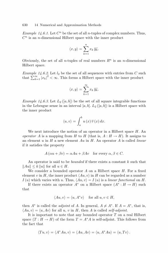
630 14 Numerical and Approximation Methods
Example 14.6.1. Let Cn be the set of all n-tuples of complex numbers. Thus,Cn is an n-dimensional Hilbert space with the inner product
〈x, y〉 =n∑
k=1
xk yk.
Obviously, the set of all n-tuples of real numbers Rn is an n-dimensionalHilbert space.
Example 14.6.2. Let l2 be the set of all sequences with entries from C suchthat
∑∞k=1 |xk|2 < ∞. This forms a Hilbert space with the inner product
〈x, y〉 =∞∑
k=1
xk yk.
Example 14.6.3. Let L2 ([a, b]) be the set of all square integrable functionsin the Lebesgue sense in an interval [a, b]. L2 ([a, b]) is a Hilbert space withthe inner product
〈u, v〉 =∫ b
a
u (x) v (x) dx.
We next introduce the notion of an operator in a Hilbert space H. Anoperator A is a mapping from H to H (that is, A : H → H). It assigns toan element u in H a new element Au in H. An operator A is called linearif it satisfies the property
A (αu + βv) = αAu + βAv for every α, β ∈ C.
An operator is said to be bounded if there exists a constant k such that‖Au‖ ≤ k ‖u‖ for all u ∈ H.
We consider a bounded operator A on a Hilbert space H. For a fixedelement v in H, the inner product 〈Au, v〉 in H can be regarded as a numberI (u) which varies with u. Thus, 〈Au, v〉 = I (u) is a linear functional on H.
If there exists an operator A∗ on a Hilbert space (A∗ : H → H) suchthat
〈Au, v〉 = 〈u, A∗v〉 for all u, v ∈ H,
then A∗ is called the adjoint of A. In general, A = A∗. If A = A∗, that is,〈Au, v〉 = 〈u, Av〉 for all u, v in H, then A is called self-adjoint.
It is important to note that any bounded operator T on a real Hilbertspace (T : H → H) of the form T = A∗A is self-adjoint. This follows fromthe fact that
〈Tu, v〉 = 〈A∗Au, v〉 = 〈Au, Av〉 = 〈u, A∗Au〉 = 〈u, Tv〉 .

14.6 Variational Methods and the Euler–Lagrange Equations 631
A self-adjoint operator A on a Hilbert space H is said to be positive if〈Au, u〉 ≥ 0 for all u in H, where equality implies that u = 0 in H. Further,if there exists a positive constant k such that 〈Au, u〉 ≥ k 〈u, u〉 for all u inH, then A is called positive definite in H.
The rest of this section is essentially concerned with linear operators ina real Hilbert space, which means that the associated scalar field involvedis real. Some specific inner products which will be used in the subsequentsections include
〈u, v〉 =∫ b
a
u (x) v (x) dx, 〈u, v〉 =∫∫
D
u (x, y) v (x, y) dx dy,
where D ⊂ R2.
Example 14.6.4. Determine whether the differentiable operators (i) A =d/dx, (ii) A = d2/dx2, and (iii) A = ∇2 =
(∂2/∂x2
)+
(∂2/∂y2
)are self-
adjoint for functions that are differentiable in a ≤ x ≤ b or in D ⊂ R2 andvanish on the boundary.
(i) 〈Au, v〉 =∫ b
a
(du
dx
)v dx =
∫ b
a
u
(−dv
dx
)dx + [u, v]ba
= 〈u, A∗v〉 where A∗ = − d
dx= A.
Hence, A is not self-adjoint.
(ii) 〈Au, v〉 =∫ b
a
(d2u
dx2
)v dx =
∫ b
a
(du
dx
)(−dv
dx
)dx +
[vdu
dx
]b
a
=∫ b
a
u
(d2v
dx2
)dx +
[vdu
dx− u
dv
dx
]b
a
=∫ b
a
u
(d2v
dx2
)dx = 〈u, Av〉 .
Thus, A is self-adjoint.
(iii) 〈Au, v〉 =∫∫
D
(∇2u)v dx dy =
∫∫D
[∇ · (∇u) v − ∇u · ∇v] dx dy
=∫
∂D
(n · ∇u) v dS −∫∫
D
∇u · ∇v dx dy
= −∫∫
D
(∇u · ∇v) dx dy,
where the divergence theorem is used with the unit outward normal vectorn.
Noting the symmetry of the right hand side in u and v, it follows that
〈Au, v〉 = 〈Av, u〉 = 〈u, Av〉 .
This means that the operator A = ∇2 is self-adjoint.
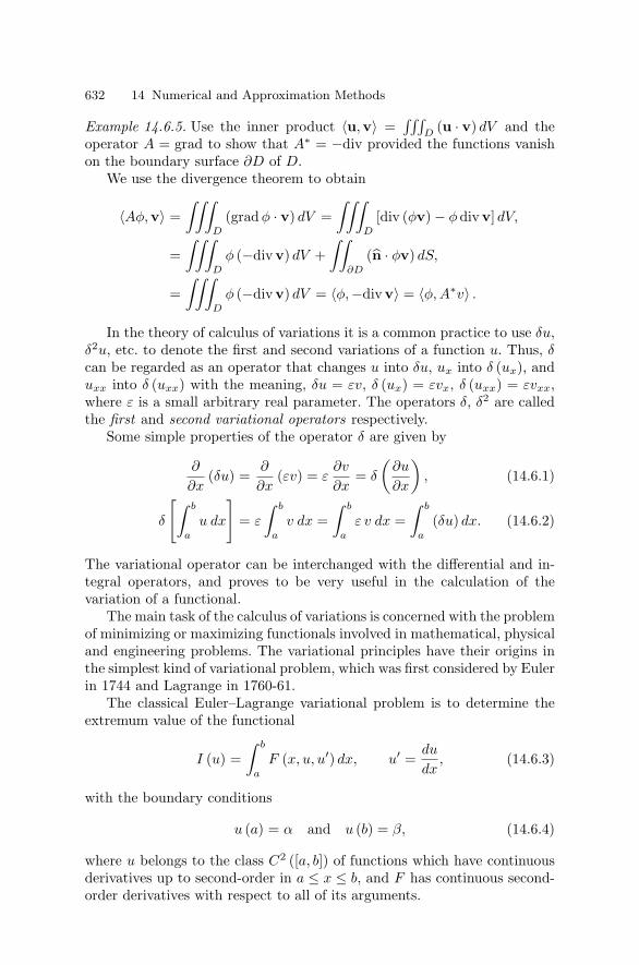
632 14 Numerical and Approximation Methods
Example 14.6.5. Use the inner product 〈u,v〉 =∫∫∫
D(u · v) dV and the
operator A = grad to show that A∗ = −div provided the functions vanishon the boundary surface ∂D of D.
We use the divergence theorem to obtain
〈Aφ,v〉 =∫∫∫
D
(gradφ · v) dV =∫∫∫
D
[div (φv) − φ divv] dV,
=∫∫∫
D
φ (−divv) dV +∫∫
∂D
(n · φv) dS,
=∫∫∫
D
φ (−divv) dV = 〈φ,−divv〉 = 〈φ, A∗v〉 .
In the theory of calculus of variations it is a common practice to use δu,δ2u, etc. to denote the first and second variations of a function u. Thus, δcan be regarded as an operator that changes u into δu, ux into δ (ux), anduxx into δ (uxx) with the meaning, δu = εv, δ (ux) = εvx, δ (uxx) = εvxx,where ε is a small arbitrary real parameter. The operators δ, δ2 are calledthe first and second variational operators respectively.
Some simple properties of the operator δ are given by
∂
∂x(δu) =
∂
∂x(εv) = ε
∂v
∂x= δ
(∂u
∂x
), (14.6.1)
δ
[∫ b
a
u dx
]= ε
∫ b
a
v dx =∫ b
a
ε v dx =∫ b
a
(δu) dx. (14.6.2)
The variational operator can be interchanged with the differential and in-tegral operators, and proves to be very useful in the calculation of thevariation of a functional.
The main task of the calculus of variations is concerned with the problemof minimizing or maximizing functionals involved in mathematical, physicaland engineering problems. The variational principles have their origins inthe simplest kind of variational problem, which was first considered by Eulerin 1744 and Lagrange in 1760-61.
The classical Euler–Lagrange variational problem is to determine theextremum value of the functional
I (u) =∫ b
a
F (x, u, u′) dx, u′ =du
dx, (14.6.3)
with the boundary conditions
u (a) = α and u (b) = β, (14.6.4)
where u belongs to the class C2 ([a, b]) of functions which have continuousderivatives up to second-order in a ≤ x ≤ b, and F has continuous second-order derivatives with respect to all of its arguments.

14.6 Variational Methods and the Euler–Lagrange Equations 633
We assume that I (u) has an extremum at some u ∈ C(2) ([a, b]). Thenwe consider the set of all variations u + εv for fixed u where v is an arbi-trary function belonging to C2 ([a, b]) such that v (a) = v (b) = 0. We nextconsider the increment of the functional
δI = I (u + εv) − I (u) =∫ b
a
[F (x, u + ε v, u′ + ε v′) − F (x, u, u′)] dx.
(14.6.5)
From the Taylor series expansion
F (x, u + ε v, u′ + ε v′) = F (x, u, u′) + ε
(v
∂F
∂u+ v′ ∂F
∂u′
)+
ε2
2!
(v
∂F
∂u+ v′ ∂F
∂u′
)2
+ · · · ,
it follows from (14.6.5) that
I (u + εv) = I (u) + ε δI +ε2
2!δ2I + · · · , (14.6.6)
where the first and second variations of I are given by
δI =∫ b
a
(v
∂F
∂u+ v′ ∂F
∂u′
)dx, (14.6.7)
δ2I =∫ b
a
(v
∂F
∂u+ v′ ∂F
∂u′
)2
dx. (14.6.8)
The necessary condition for the functional I (u) to have an extremum (thatis, I (u) is stationary at u) is that the first variation becomes zero at u so
0 = δI =∫ b
a
(v
∂F
∂u+ v′ ∂F
∂u′
)dx (14.6.9)
which is, by partial integration of the second integral,
=∫ b
a
[∂F
∂u− d
dx
(∂F
∂u′
)]v dx +
[v
∂F
∂u′
]b
a
.
Because v (a) = v (b) = 0, this means that∫ b
a
[∂F
∂u− d
dx
(∂F
∂u′
)]v dx = 0. (14.6.10)
Since v is arbitrary in a ≤ x ≤ b, it follows from (14.6.10) that
∂F
∂u− d
dx
(∂F
∂u′
)= 0. (14.6.11)
This is the famous Euler–Lagrange equation. We therefore can state:

634 14 Numerical and Approximation Methods
Theorem 14.6.1. A necessary condition for the functional I (u) to be sta-tionary at u is that u is a solution of the Euler–Lagrange equation
∂F
∂u− d
dx
(∂F
∂u′
)= 0, a ≤ x ≤ b (14.6.12)
with
u (a) = α, u (b) = β. (14.6.13)
This is called the Euler–Lagrange variational principle.
Note that, in general, equation (14.6.12) is a nonlinear second-orderordinary differential equations, and, although such an equation is very dif-ficult to solve, still it seems to be more accessible analytically than thefunctional (14.6.3) from which it is derived.
The derivative ddx in (14.6.12) can be computed by recalling u = u (x)
and u′ = dudx , and equation (14.6.12) becomes
∂F
∂u− ∂2F
∂x∂u′ − ∂2F
∂u∂u′
(du
dx
)− ∂2F
∂u′2d2u
∂x2 = 0.
It is left to the reader to verify that the functional with one independentvariable and nth-order derivatives in the form
I (u) =∫ b
a
F (x, u, ux, uxx, . . . , uxn , . . . , ) dx
admits the Euler–Lagrange equation
∂F
∂u− d
dx
(∂F
∂ux
)+
d2
dx2
(∂F
∂uxx
)− . . . (−1)n dn
dxn
(∂2F
∂uxn
)= 0.
After we have determined the function u which makes I (u) stationary,the question of the nature of the extremum arises, that is, its minimum,maximum, or saddle point properties. To answer this question, we look atthe second variation defined in (14.6.8). If terms of O
(ε3
)can be neglected
in (14.6.6), or if they vanish for the case of quadratic F , it follows from(14.6.6) that a necessary condition for the functional I (u) to have a mini-mum I (u) ≥ I (u0) at u = u0 is that δ2I ≥ 0, for I (u) to have a maximumI (u) ≤ I (u0) at u = u0 is that δ2I ≤ 0 at u = u0 respectively for alladmissible values of v. These results enable us to determine the upper orlower bounds for the stationary value I (u0) of the functional.
Example 14.6.6. Find out the shortest distance between given points A andB in the (x, y)-plane.
Suppose APB is any curve in the plane through A and B, and s =arcAP . The problem is to determine the curve for which the functional

14.6 Variational Methods and the Euler–Lagrange Equations 635
I (y) =∫ B
A
ds, (14.6.14)
is a minimum.Since ds/dx =
(1 + y′2) 1
2 , functional (14.6.14) becomes
I (y) =∫ x2
x1
(1 + y′2) 1
2 dx. (14.6.15)
In this case, F =(1 + y′2) 1
2 which depends on y′ only, so ∂F/∂y = 0.Hence, the Euler–Lagrange equation (14.6.12) becomes
d
dx
(∂F
∂y′
)= 0.
This gives the differential equation
y′′ = 0. (14.6.16)
This means that the curvature for all points on the curve AB is zero. Hence,the path AB is a straight line. It follows from the integration of (14.6.16)that y = mx + c is a two-parameter family of straight lines.
Example 14.6.7. (Fermat principle in optics). In an optically homogeneousisotro-pic medium, light travels from one point A to another point B alongthe path for which the travel time is minimum.
The velocity of light v is the same at all points of the medium; hence, theminimum time is equivalent to the minimum path length. For simplicity,consider a path joining the two points A and B in the (x, y)-plane. Thetime to travel an elementary arc length ds is ds/v. Thus, the variationalproblem is to find the path for which∫ B
A
ds
v=
∫ x2
x1
(1 + y′2) 1
2 dx
v=
∫ x2
x1
F (y, y′) dx (14.6.17)
is a minimum, where y′ = dy/dx, and v = v (y).When F is a function of y and y′, the Euler–Lagrange equation (14.6.12)
becomesd
dx(F − y′Fy′) = 0. (14.6.18)
This follows from the resultd
dx(F − y′Fy′) =
d
dxF (y, y′) − y′′Fy′ − y′ d
dx(Fy′)
= y′Fy + y′′Fy − y′′Fy − y′ d
dx(Fy′)
= y′[Fy − d
dx(Fy′)
]= 0, by (14.6.12) .

636 14 Numerical and Approximation Methods
Hence,
F − y′Fy′ = constant, (14.6.19)
or (1 + y′2) 1
2
v− y′2
v (1 + y′2)12
= constant,
or
v−1 (1 + y′2)− 1
2 = constant. (14.6.20)
In order to give a simple physical interpretation, we rewrite (14.6.20) interms of the angle φ made by the tangent to the minimum path with thevertical y-axis so that
sin φ =(1 + y′2)− 1
2 .
Hence,
1v
sin φ = constant = K (14.6.21)
for all points on the minimum curve. For a ray of light, (1/v) must bedirectly proportional to the refractive index n of the medium through whichlight is travelling. Equation (14.6.21) is called the Snell law of refraction oflight. Often this law is stated as
n sin φ = constant. (14.6.22)
(A) Hamilton Principle
The difference between the kinetic energy T and the potential energy Vof a dynamical system is denoted by L = T − V . The quantity L is calledthe Lagrangian of the system. The Hamilton principle states that the firstvariation of the time integral of L is zero, that is,
δ
∫ t2
t1
L dt = δ
∫ t2
t1
(T − V ) dt = 0. (14.6.23)
This result is supposed to be valid for all dynamical systems whether theyare conservative or nonconservative.
For a conservative system the force field F = −∇V and T + V = C,where C is a constant, and so (14.6.23) gives the principle of least action
δA = 0, A =∫ t2
t1
L dt, (14.6.24)
where A is called the action integral or simply the action of the system.

14.6 Variational Methods and the Euler–Lagrange Equations 637
Example 14.6.8. Derive the Newton second law of motion from the Hamil-ton principle.
Consider a particle of mass m at the position r = (x, y, z) which ismoving under the action of a field of force F. The kinetic energy of theparticle is T = 1
2mr2, and the variation of work done is δW = F · δr andδV = −δW . Thus, the Hamilton principle for the system is
0 = δ
∫ t2
t1
(T − V ) dt =∫ t2
t1
(δT − δV ) dt =∫ t2
t1
(mr · δr + F · δr) dt.
Integrating this result by parts and noting that δr vanishes at t = t1and t = t2, we obtain ∫ t2
t1
(mr − F) · δr dt = 0.
This is true for every virtual displacement δr, and hence, the integrandmust vanish, that is,
mr = F. (14.6.25)
This is the celebrated Newton second law of motion.
Example 14.6.9. Derive the equation for a simple harmonic oscillator in anon-resisting medium from the Hamilton principle.
For a simple harmonic oscillator, T = 12mx2 and V = 1
2mω2x2. Accord-ing to the Hamilton principle
δ
∫ t2
t1
(12mx2 − 1
2mω2x2
)dt = δ
∫ t2
t1
F (x, x) dt = 0.
This leads to the Euler–Lagrange equation
∂F
∂x− d
dt(mx) = 0,
or
x + ω2x = 0. (14.6.26)
This is the equation for the simple harmonic oscillator.
Example 14.6.10. A straight uniform elastic beam of length l, line density ρ,cross-sectional moment of inertia I, and modulus of elasticity E is fixed ateach end. The beam performs small transverse oscillations in the horizontal(x, y)-plane. Derive the equation of motion of the beam.
The potential energy of the elastic beam is
V =12
∫ l
0
M2
EIdx =
12
∫ l
0EIy′′2dx,

638 14 Numerical and Approximation Methods
where the bending moment M is proportional to the curvature so that
M = EIy′′
(1 + y′2)12
∼ EIy′′ for small y′.
The variational principle gives
δ
∫ t2
t1
(T − V ) dt = δ
∫ t2
t1
F (y′′, y) dt = 0,
where
F (y′′, y) =12
∫ l
0
(ρy2 − EIy′′2) dx.
This principle leads to the Euler–Lagrange equation
−∫ l
0
(ρy + EIy(iv)
)dx = 0,
or
ρy + EIy(iv) = 0. (14.6.27)
This represents the partial differential equation of the transverse vibrationof the beam.
(B) The Generalized Coordinates, Lagrange Equation, andHamilton Equation
The Euler–Lagrange analysis of a dynamical system can be extended tomore complex cases where the configuration of the system is described bygeneralized coordinates q1, q2, . . ., qn. Without loss of generality, we considera system of three variables where the familiar Cartesian coordinates x, y,z can be expressed in terms of the generalized coordinates q1, q2, q3 as
x = x (q1, q2, q3) , y = y (q1, q2, q3) , z = z (q1, q2, q3) . (14.6.28)
For example, if (q1, q2, q3) represents the cylindrical polar coordinates(r, θ, z), the above result becomes
x = r cos θ, y = r sin θ, z = z.
Since the coordinates are functions of time t, we obtain the followingresult by differentiation
x =∂x
∂q1q1 +
∂x
∂q2q2 +
∂x
∂q3q3 (14.6.29)
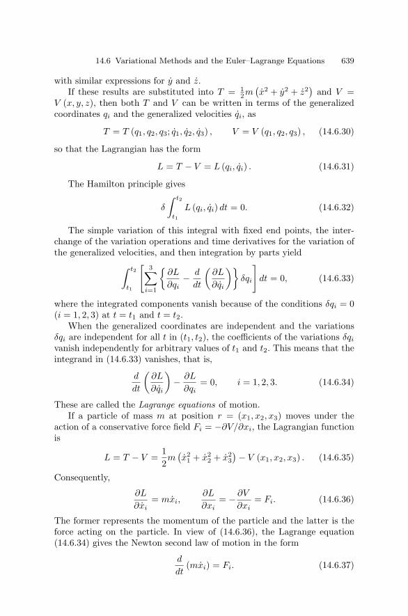
14.6 Variational Methods and the Euler–Lagrange Equations 639
with similar expressions for y and z.If these results are substituted into T = 1
2m(x2 + y2 + z2
)and V =
V (x, y, z), then both T and V can be written in terms of the generalizedcoordinates qi and the generalized velocities qi, as
T = T (q1, q2, q3; q1, q2, q3) , V = V (q1, q2, q3) , (14.6.30)
so that the Lagrangian has the form
L = T − V = L (qi, qi) . (14.6.31)
The Hamilton principle gives
δ
∫ t2
t1
L (qi, qi) dt = 0. (14.6.32)
The simple variation of this integral with fixed end points, the inter-change of the variation operations and time derivatives for the variation ofthe generalized velocities, and then integration by parts yield∫ t2
t1
[3∑
i=1
∂L
∂qi− d
dt
(∂L
∂qi
)δqi
]dt = 0, (14.6.33)
where the integrated components vanish because of the conditions δqi = 0(i = 1, 2, 3) at t = t1 and t = t2.
When the generalized coordinates are independent and the variationsδqi are independent for all t in (t1, t2), the coefficients of the variations δqi
vanish independently for arbitrary values of t1 and t2. This means that theintegrand in (14.6.33) vanishes, that is,
d
dt
(∂L
∂qi
)− ∂L
∂qi= 0, i = 1, 2, 3. (14.6.34)
These are called the Lagrange equations of motion.If a particle of mass m at position r = (x1, x2, x3) moves under the
action of a conservative force field Fi = −∂V/∂xi, the Lagrangian functionis
L = T − V =12m
(x2
1 + x22 + x2
3) − V (x1, x2, x3) . (14.6.35)
Consequently,
∂L
∂xi= mxi,
∂L
∂xi= − ∂V
∂xi= Fi. (14.6.36)
The former represents the momentum of the particle and the latter is theforce acting on the particle. In view of (14.6.36), the Lagrange equation(14.6.34) gives the Newton second law of motion in the form
d
dt(mxi) = Fi. (14.6.37)

640 14 Numerical and Approximation Methods
Example 14.6.11. Apply the Lagrange equations of motion to derive theequations of motion of a particle under the action of a central force,−mF (r) where r is the distance of the particle of mass m from the centerof force.
It is convenient to use the polar coordinates r and θ. In terms of thegeneralized coordinates q1 = r and q2 = θ, we write
x = r cos θ = q1 cos q2, y = r sin θ = q1 sin q2.
The kinetic energy T is
T =12m
(x2 + y2) =
12m
(r2 + r2θ2
)=
12m
(q21 + q2
1 q22). (14.6.38)
Since F = ∇V , the potential is
V (r) =∫ r
F (r) dr =∫ q1
F (q1) dq1. (14.6.39)
Then, the Lagrangian L is
L = T − V =12m
[(q21 + q2
1 q22) − 2
∫ q1
F (q1) dq1
]. (14.6.40)
Thus, the Lagrange equations (14.6.34) with i = 1, 2, 3 give the equationsof motion
q1 − q1q22 + F (q1) = 0,
d
dt
(q21 q2
)= 0. (14.6.41)
In term of the polar coordinates, these equations become
r − rθ2 = −F (r) ,d
dt
(r2θ
)= 0. (14.6.42ab)
Equation (14.6.42b) gives immediately
r2θ = h, (14.6.43)
where h is a constant. In this case, rθ represents the transverse velocitycomponent, and mr2θ = mh is the constant angular momentum of theparticle about the center of force.
Introducing r = 1/u, we obtain
r =dr
dt= − 1
u2
du
dt= − 1
u2
du
dθ· dθ
dt= −h
du
dθ,
r =d2r
dt2= −h
d
dt
(du
dθ
)= −h
d2u
dθ2
dθ
dt= −h2u2 d2u
dθ2 .
Substituting these into (14.6.42a) gives

14.6 Variational Methods and the Euler–Lagrange Equations 641
−h2u2 d2u
dθ2 − h2u3 = −F
(1u
),
or
d2u
dθ2 + u =1
h2u2 F
(1u
). (14.6.44)
This is the differential equation of the central orbit and can be solved bystandard methods.
In particular, if the law of force is the attractive inverse square, F (r) =µ/r2 so that the potential V (r) = −µ/r, the differential equation (14.6.44)becomes
d2u
dθ2 + u =µ
h2 , (14.6.45)
if the particle is projected initially from distance a with velocity V at anangle β that the direction of motion makes with the outward radius vector.Thus, the constant h in (14.6.43) is h = V a sin β. The angle φ between thetangent and radius vector of the orbit at any point is given by
cot φ =1r
dr
dθ= u
d
dθ
(1u
)= − 1
u
du
dθ. (14.6.46)
At t = 0, the initial conditions are
u =1a,
du
dθ= −1
acot β when θ = 0. (14.6.47)
The general solution of equation (14.6.45) is
u =µ
h2 [1 + e cos (θ + α)] , (14.6.48)
where e and α are constants to be determined from the initial data.Finally, the solution can be written as
l
r= 1 + e cos (θ + α) , (14.6.49)
where
l =h2
µ= (V a sin β)2 /µ. (14.6.50)
This represents a conic section of semi-latus rectum l and eccentricitye with its axis inclined at an angle α to the radius vector at the point ofprojection.
The initial conditions (14.6.47) lead to

642 14 Numerical and Approximation Methods
l
a= 1 + e cos α, − l
acot β = −e sin α, (14.6.51)
which give
tanα =l cot β
l − a,
e2 =(
l
a− 1
)2
+l2
a2 cot2 β =l2
a2 cosec2β − 2l
a+ 1,
= 1 − 2aV 2 sin2 β
µ+
a2V 4 sin2 β
µ2 . (14.6.52)
Thus, the conic is an ellipse, parabola, or hyperbola accordingly as e <=> 1that is, V 2 < = > 2µ/a.
To derive the Hamilton equations, we introduce the concept of general-ized momentum, pi and generalized force, Fi as
pi =∂L
∂qi, Fi =
∂L
∂qi. (14.6.53ab)
Consequently, the Lagrange equations (14.6.34) become
∂L
∂qi=
d
dtpi = pi. (14.6.54)
The Hamiltonian function H is defined by
H =n∑
i=1
pi qi − L. (14.6.55)
In general, L = L (qi, qi, t) is a function of qi, qi and t, where qi entersthrough the kinetic energy as a quadratic term. Hence, equation (14.6.53a)will give pi as a linear function of qi. This system of linear equations in-volving pi and qi can be solved to determine qi in terms of pi, and then, theqi can, in principle, be eliminated from (14.6.55). This means that H canalways be expressed as a function of pi, qi and t so that H = H (pi, qi, t).Thus,
dH =∑ ∂H
∂pidpi +
∑ ∂H
∂qidqi +
∂H
∂tdt. (14.6.56)
On the other hand, differentiating H in (14.6.55) with respect to t gives
dH
dt=
∑pi
d
dtqi +
∑qi
d
dtpi −
∑ ∂L
∂qi
d
dtqi −
∑ ∂L
∂qi
d
dtqi − ∂L
∂t,
(14.6.57)
or

14.6 Variational Methods and the Euler–Lagrange Equations 643
dH =∑
pi dqi +∑
qi dpi −∑ ∂L
∂qidqi −
∑ ∂L
∂qidqi − ∂L
∂tdt, (14.6.58)
which becomes, in view of (14.6.53a),
dH =∑
qi dpi −∑ ∂L
∂qidqi − ∂L
∂tdt. (14.6.59)
Evidently, two expressions of dH in (14.6.56) and (14.6.59) must beequal so that the coefficients of the corresponding differentials can beequated to obtain
qi =∂H
∂pi, − ∂L
∂qi=
∂H
∂qi, −∂L
∂t=
∂H
∂t. (14.6.60abc)
Using the Lagrange equation (14.6.54), the first two of the above equationsbecome
qi =∂H
∂pi, pi = −∂H
∂qi. (14.6.61ab)
These are commonly known as the Hamilton canonical equations of motion.They play a fundamental role in advanced analytical dynamics.
Finally, the Lagrange–Hamilton theory can be used to derive the lawof conservation of energy. In general, the Lagrangian L is independent oftime t and hence, (14.6.60c) implies that H = constant. Again, T involvedin L = T − V is given by
T =12
n∑i=1
n∑j=1
aij qi qj , (14.6.62)
where the coefficients aij are symmetric functions of the generalized coor-dinates qij , that is, aij = aji.
On the other hand, V is, in general, independent of qi and hence,
pi =∂L
∂qi=
∂T
∂qi=
n∑j=1
aij qj . (14.6.63)
Thus, the Hamiltonian H becomes
H =n∑
i=1
piqi − L =n∑
i=1
⎛⎝ n∑j=1
aij qj
⎞⎠ qi − L = 2T − L = T + V. (14.6.64)
Thus, H is equal to the total energy. It has already been observed that,if L does not contain t explicitly, H is a constant. This means that thesum of the potential and kinetic energies is constant. This is the law of theconservation of energy.

644 14 Numerical and Approximation Methods
Example 14.6.12. Use the Hamiltonian equations to derive the equations ofmotion for the problem stated in Example 14.6.11.
The Lagrangian L for this problem is given by (14.6.40) with q1 = rand q2 = θ. It follows from the definition (14.6.53a) of the generalizedmomentum that
p1 = mq1 = mr, p2 = mq21 q2 = mr2θ. (14.6.65)
Expressing the results of the kinetic energy (14.6.38) and the potentialenergy (14.6.39) in terms of p1 and p2 the Hamiltonian H = T + V can bewritten as
H =1
2m
(p21 +
p22
q21
)+ m
∫ q1
F (q1) dq1. (14.6.66)
Then, equations (14.6.65) and the Hamilton equation (14.6.61b) give
p1 = mr, p2 = mr2θ, (14.6.67)
p1 =1m
p22
q31
+ mF (q1) , p2 = 0. (14.6.68)
Clearly, these equations are identical with the equations of motion(14.6.42ab).
Example 14.6.13. Derive the equation of a simple pendulum by using (i) theLagrange equations and (ii) the Hamilton equations.
We consider the motion of simple pendulum of mass m attached at theend of a rigid massless string of length l that pivots about a fixed point.We suppose that the pendulum makes an angle θ with its vertical position.The force F acting on the mass m is F = −mg sin θ, so that the potentialV is obtained from F = −∇V as V = mgl (1 − cos θ). The kinetic energyT = 1
2ml2θ2.Thus the Lagrangian L is
L = T − V =12ml2θ2 − mgl (1 − cos θ) = L
(θ, θ
). (14.6.69)
The Lagrange equation is
∂L
∂θ− d
dt
(∂L
∂θ
)= 0, (14.6.70)
or
−mgl sin θ − d
dt
(ml2θ
)= 0,
or
θ + ω2 sin θ = 0, ω2 = g/l. (14.6.71ab)

14.6 Variational Methods and the Euler–Lagrange Equations 645
This is the equation of the simple pendulum.To derive the same equation from the Hamilton equations, we choose
q1 = l (q1 = 0) and q2 = θ as the generalized (polar) coordinates. Thekinetic and potential energies are
T =12ml2q2
2 , V = mgl (1 − cos q2) . (14.6.72ab)
Thus, H = T + V and L = T − V are given by
(H, L) =12ml2q2
2 + mgl (1 − cos q2) . (14.6.73ab)
From the definition of the generalized momentum, we find that
p2 =∂L
∂q2= ml2q2
so that the Hamiltonian H in terms of p2 and q2 is
H =12
p22
ml2+ mgl (1 − cos q2) .
Thus, the Hamilton equation (14.6.61ab) gives
θ + ω2 sin θ = 0, ω2 =g
l. (14.6.74)
The variational methods can be further extended for functionals de-pending on functions or more independent variables in the form
I [u (x, y)] =∫∫
D
F (x, y, u, ux, uy) dx dy (14.6.75)
where the values of the function u (x, y) are prescribed on the boundary∂D of a finite domain D in the (x, y)-plane. We assume that F is differen-tiable and the surface u = u (x, y) giving an extremum is also continuouslydifferentiable twice.
The first variation δI of I is defined by
δI [u, ε] = I (u + ε) − I (u) (14.6.76)
which is, by Taylor’s expansion theorem
=∫∫
D
[εFu + εxFp + εyFq] dx dy (14.6.77)
where ε ≡ ε (x, y) is small and p = ux and q = uy. According to thevariational principle, δI = 0 for all admissible values of ε. The partialintegration of (14.6.77) combined with ε = 0 on ∂D gives

646 14 Numerical and Approximation Methods
0 = δI =∫∫
D
[Fu − ∂
∂xFp − ∂
∂yFq
]ε (x, y) dx dy. (14.6.78)
This is true for all arbitrary ε, and hence, the integrand must vanish, thatis
∂
∂xFp +
∂
∂yFq − Fu = 0. (14.6.79)
This is the Euler–Lagrange equation which is the second-order partial dif-ferential equation to be satisfied by the extremizing function u (x, y).
Example 14.6.14. Derive the equation of motion for the free vibration of anelastic string of length l.
The potential energy V of the string is
V =12T ∗
∫ l
0u2
xdx (14.6.80)
where u = u (x, y) is the displacement of the string from its equilibriumposition and T ∗ is the constant tension of the string.
The kinetic energy T is
T =12
∫ l
0ρu2
t dx (14.6.81)
where ρ is the constant line-density of the string.According to the Hamilton principle
δI = δ
∫ t2
t1
(T − V ) dt = δ
∫ t2
t1
∫ l
0
12(ρu2
t − T ∗u2x
)dx dt = 0 (14.6.82)
which has the form
δ
∫ t2
t1
∫ l
0L (ut, ux) = 0, (14.6.83)
where
L =12(ρ u2
t − T ∗u2x
).
Then the Euler–Lagrange equation is given by
∂
∂t(ρut) − ∂
∂x(T ∗ux) = 0, (14.6.84)
or
utt − c2uxx = 0, c2 = T ∗/ρ. (14.6.85)
This is the wave equation of motion of the string.

14.7 The Rayleigh–Ritz Approximation Method 647
Example 14.6.15. Derive the Laplace equation from the functional
I (u) =∫∫
D
(u2
x + u2y
)dx dy
with a boundary condition u = f (x, y) on ∂D.The variational principle gives
δI = δ
∫∫D
(u2
x + u2y
)dx dy = 0.
This leads to the Euler–Lagrange equation
uxx + uyy = 0 in D.
Similarly, the functional
I [u (x, y, z)] =∫∫∫
D
(u2
x + u2y + u2
z
)dx dy dz
will lead to the three-dimensional Laplace equation
∇2u = uxx + uyy + uzz = 0.
14.7 The Rayleigh–Ritz Approximation Method
We consider the boundary-value problem governed by the differential equa-tion
Au = f in D (14.7.1)
with the boundary condition
B (u) = 0 on ∂D (14.7.2)
where A is a self-adjoint differential operator in a Hilbert space H andf ∈ H.
In general, the determination of the exact solution of the problem is of-ten a difficult task. However, it can be shown that the solution of (14.7.1)–(14.7.2) is equivalent to finding the minimum of a functional I (u) associatedwith the differential system. In other words, the solution can be character-ized as the function which minimizes (or maximizes) the functional I (u). Asimple and efficient method for an approximate solution of the extremumproblem was independently formulated by Lord Rayleigh and W. Ritz.
We next prove a fundamental result which states that the solution ofthe equation (14.7.1) is equivalent to finding the minimum of the quadraticfunctional

648 14 Numerical and Approximation Methods
I (u) ≡ A 〈u, u〉 − 2 〈f, u〉 . (14.7.3)
Suppose that u = u0 is the solution of (14.7.1) so that Au0 = f . Conse-quently,
I (u) ≡ A 〈u, u〉 − 2 〈Au0, u〉 = 〈A (u − u0) , u〉 − 〈Au0, u〉 .
Since the inner product is symmetrical and 〈Au0, u〉 = 〈u0, Au〉 =〈Au, u0〉, I (u) can be written as
I (u) = 〈A (u − u0) , u〉 − 〈Au, u0〉 + 〈Au0, u〉 − 〈Au0, u0〉 ,
= 〈A (u − u0) , u − u0〉 − 〈Au0, u0〉 ,
= 〈A (u − u0) , u − u0〉 + I (u0) . (14.7.4)
Since A is a positive operator, 〈A (u − u0) , u − u0〉 ≥ 0 where equalityholds if and only if u − u0 = 0. It follows that
I (u) ≥ I (u0) , (14.7.5)
where equality holds if and only if u = u0. We conclude from this inequalitythat I (u) assumes its minimum at the solution u = u0 of equation (14.7.1).
Conversely, the function u = u0 that minimizes I (u) is a solution ofequation (14.7.1). Clearly, I (u) ≥ I (u0), that is, in particular, I (u0 + αv) ≥I (u0) for any real α and any function v. Explicitly,
I (u0 + αv) = 〈A (u0 + αv) , u0 + αv〉 − 2 〈f, u0 + αv〉 ,
= 〈Au0, u0〉 + 2α 〈Au0, v〉 + α2 〈Av, v〉 − 2 〈f, u0〉 − 2α 〈f, v〉 .
This means that I (u0 + αv) is a quadratic expression in α. Since I (u) isminimum at u = u0, then δI (u0, v) = 0, that is,
0 =[
d
dαI (u0 + αv)
]α=0
= 2 〈Au0, v〉 − 2 〈f, v〉= 2 〈Au0 − f, v〉 .
This is true for any arbitrary but fixed v. Hence, Au0 − f = 0. This provesthe assertion.
In the Rayleigh–Ritz method an approximate solution of (14.7.1)–(14.7.2) is sought in the form
un (x) =n∑
i=1
aiφi (x) , (14.7.6)
where a1, a2, . . ., an are n unknown coefficients to be determined so thatI (un) is minimum, and φ1, φ2, . . ., φn represent a linearly independent and

14.7 The Rayleigh–Ritz Approximation Method 649
complete set of arbitrarily chosen functions that satisfy (14.7.2). This setof functions is often called a trial set. We substitute (14.7.6) into (14.7.3)to obtain
I (un) =
⟨n∑
i=1
aiA (φi) ,
n∑j=1
ajφj
⟩− 2
⟨f,
n∑i=1
aiφi
⟩.
Then the necessary condition for I to obtain a minimum (or maximum) isthat
∂I
∂aj(a1, a2, . . . , an) = 0, j = 1, 2, . . . , n, (14.7.7)
or
∂I
∂aj
⎡⎣⟨n∑
i=1
aiA (φi) ,
n∑j=1
ajφj
⟩− 2
⟨f,
n∑i=1
aiφi
⟩⎤⎦ = 0,
orn∑
i=1
〈A (φi) , φj〉 ai +n∑
i=1
〈A (φj) , φi〉 aj − 2 〈f, φj〉 = 0,
or
2n∑
i=1
〈A (φi) , φj〉 ai = 2 〈f, φj〉 .
Therefore,
n∑i=1
〈A (φi) , φj〉 ai = 〈f, φj〉 , j = 1, 2, . . . , n. (14.7.8)
This is a linear system of n equations for the n unknown coefficients aj .Once a1, a2, . . ., an are determined, the approximate solution is given by(14.7.6).
In particular, when
〈A (φi) , φj〉 =
⎧⎨⎩0, i = j
1, i = j,(14.7.9)
equation (14.7.8) gives aj as
aj = 〈φj , f〉 , (14.7.10)
so that the Rayleigh–Ritz approximate series (14.7.6) becomes

650 14 Numerical and Approximation Methods
un (x) =n∑
i=1
〈φi, f〉φi (x) . (14.7.11)
This is similar to the Fourier series solution with known Fourier coefficientsai.
In the limit n → ∞, a limit function can be obtained from (14.7.6) as
u (x) = limn→∞
n∑i=1
ai φi (x) =∞∑
i=1
ai φi (x) , (14.7.12)
provided that the series converges. Under certain assumptions imposed onthe functional I (u) and the trial functions φ1, φ2, . . ., φn, the limit functionu (x) represents an exact solution of the problem. In any event, (14.7.6) or(14.7.11) gives a reasonable approximate solution.
In the simplest case corresponding to n = 1, the Rayleigh–Ritz methodgives a simple form of the functional
I (u1) = I (a1φ1) = a21 〈Aφ1, φ1〉 − 2a1 〈f, φ1〉 ,
where a1 is readily determined from the necessary condition for extremum
0 =∂
∂a1I (a1φ1) = 2a1 〈Aφ1, φ1〉 − 2 〈f, φ1〉 ,
or
a1 =〈f, φ1〉
〈Aφ1, φ1〉 . (14.7.13)
The corresponding minimum value of the functional is given by
I (a1φ1) = − 〈f, φ1〉2〈Aφ1, φ1〉 . (14.7.14)
Thus, the essence of the Rayleigh–Ritz method is as follows. For a givenboundary-value problem, an approximate series solution is sought so thatthe trial functions φi satisfy the boundary conditions. We solve the systemof algebraic equations (14.7.7) to determine the coefficients ai.
We now illustrate the method by several examples.
Example 14.7.1. Find an approximate solution of the Dirichlet problem
∇2u ≡ uxx + uyy = 0 in D
u = f on ∂D,
where D ⊂ R2, and f is a given function.This problem is equivalent to finding the minimum of the associated
functional

14.7 The Rayleigh–Ritz Approximation Method 651
I (u) =∫∫
D
(u2
x + u2y
)dx dy.
We seek an approximate series solution in the form
u2 (x, y) = a1φ1 + a2φ2
with a1 = 1 so that u2 satisfies the given boundary conditions, that is,φ1 = f and φ2 = 0 on ∂D. Substituting u2 into the functional gives
I (u2) =∫∫
D
[(∂u2
∂x
)2
+(
∂u2
∂y
)2]
dx dy
=∫∫
D
(∇φ1)2dx dy + 2a2
∫∫D
(∇φ1 · ∇φ2) dx dy
+ a22
∫∫D
|∇φ2|2 dx dy.
The necessary condition for an extremum of I (u2) is
∂I
∂a2= 0,
or
2∫∫
D
(∇φ1 · ∇φ2) dx dy + 2a2
∫∫D
|∇φ2|2 dx dy = 0.
Therefore,
a2 = −∫∫
(∇φ1 · ∇φ2) dx dy∫∫ |∇φ2|2 dx dy.
This a2 minimizes the functional and the approximate solution is obtained.However, this procedure can be generalized by seeking an approximate
solution in the form
un =n∑
i=1
aiφi (a1 = 1)
so that φ1 = f and φi = 0 (i = 2, 3, . . . , n) on ∂D.The coefficients ai can be obtained by solving the system (14.7.7) with
j = 2, 3, . . ., n.
Example 14.7.2. A uniform elastic beam of length l carrying a uniform loadW per unit length is freely hinged at x = 0 and x = l. Find the approximatesolution of the boundary-value problem
EI(iν)y (x) = W,
y = y′′ = 0 at x = 0 and x = l,
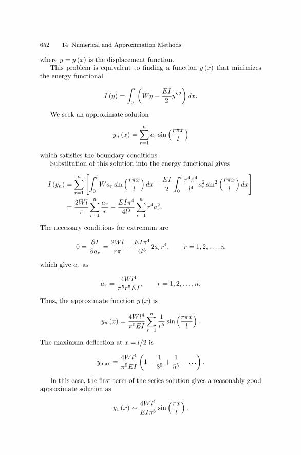
652 14 Numerical and Approximation Methods
where y = y (x) is the displacement function.This problem is equivalent to finding a function y (x) that minimizes
the energy functional
I (y) =∫ l
0
(Wy − EI
2y′′2
)dx.
We seek an approximate solution
yn (x) =n∑
r=1
ar sin(rπx
l
)which satisfies the boundary conditions.
Substitution of this solution into the energy functional gives
I (yn) =n∑
r=1
[∫ l
0War sin
(rπx
l
)dx − EI
2
∫ l
0
r4π4
l4a2
r sin2(rπx
l
)dx
]
=2Wl
π
n∑r=1
ar
r− EIπ4
4l3
n∑r=1
r4a2r.
The necessary conditions for extremum are
0 =∂I
∂ar=
2Wl
rπ− EIπ4
4l32arr
4, r = 1, 2, . . . , n
which give ar as
ar =4Wl4
π5r5EI, r = 1, 2, . . . , n.
Thus, the approximate function y (x) is
yn (x) =4Wl4
π5EI
n∑r=1
1r5 sin
(rπx
l
).
The maximum deflection at x = l/2 is
ymax =4Wl4
π5EI
(1 − 1
35 +155 − . . .
).
In this case, the first term of the series solution gives a reasonably goodapproximate solution as
y1 (x) ∼ 4Wl4
EIπ5 sin(πx
l
).

14.7 The Rayleigh–Ritz Approximation Method 653
Example 14.7.3. Apply the Rayleigh–Ritz method to investigate the freevibration of a fixed elastic wedge of constant thickness governed by theenergy functional
I (y) =∫ 1
0
(αx3y′′2 − ωxy2) dx, y (1) = y′′ (1) = 0,
where the free vibration is described by the function u (x, t) = eiωty (x), ωis the frequency.
We seek an approximate solution in the form
yn (x) =n∑
r=1
aryr (x) =n∑
r=1
ar (x − 1)2 xr−1
which satisfies the given boundary conditions.We take only the first two terms so that y2 (x) = a1y1 +a2y2 = (x − 1)2
(a1 + a2x). Substituting y2 into the functional we obtain
I2 = I (y2) =∫ 1
0
[αx3 (6a2x + 2a1 − 4a2)
2 − ωx (x − 1)4 (a1 + a2x)2]dx
= α
[(a1 − 2a2)
2 +245
(a1 − 2a2) a2 + 6a22
]− ω
5
[a21
6+
2a1a2
21+
a22
56
].
The necessary conditions for an extremum are
∂I2
∂a1= 2a1
(α − ω
30
)+
25
a2
(2α − ω
21
)= 0,
∂I2
∂a2=
2a1
5
(2α − ω
21
)+
2a2
5
(2α − ω
56
)= 0.
For nontrivial solutions, the determinant of this algebraic system must bezero, that is, ∣∣∣∣∣∣
α − ω30
15
(2α − ω
21
)2α − ω
21 2α − ω56
∣∣∣∣∣∣ = 0,
or
5(α − ω
30
)(2α − ω
56
)−
(2α − ω
21
)2= 0.
This represents the frequency equation of the vibration which has two rootsω1 and ω2. The smaller of these two frequencies gives an approximate valueof the fundamental frequency of the vibration of the wedge.
Example 14.7.4. An elastic beam of length l, density ρ, cross-sectional areaA, and modulus of elasticity E has its end x = 0 fixed and the other end

654 14 Numerical and Approximation Methods
connected to a rigid support through a linear elastic spring with springconstant k. Apply the Rayleigh–Ritz method to investigate the harmonicaxial motion of the beam.
The kinetic energy and the potential energy associated with the axialmotion of the beam are
T =∫ l
0
ρA
2U2
t dx, V =∫ l
0
EA
2U2
x dx +k
2U2 (l, t) ,
where U (x, t) is the displacement function.Since the axial motion is simple harmonic, U (x, t) = u (x) eiωt, where
ω is the frequency of vibration. Consequently, the expressions for T and Vcan be written in terms of u (x). We then apply the Hamilton variationalprinciple
δI (u) = δ
[∫ t2
t1
∫ l
0
12(ρ A ω2 u2 − EA u2
x
)dx − k
2u2 (l)
]dt = 0.
The Euler–Lagrange equation for the variational principle is
d
dx
(EA
du
dx
)+ ρ A ω2 u = 0, 0 < x < l,
EAdu
dx+ ku = 0, at x = l.
In terms of nondimensional variables (x∗, u∗) = (1/l) (x, u) and parame-ters λ =
(ω2ρl2/E
)and α = (kl/EA), this system becomes, dropping the
asterisks,
uxx + λu = 0, 0 < x < 1,
ux + α u = 0, at x = 1.
The associated functional for the system is
I (u) =12
∫ 1
0
(λu2 − u2
x
)dx − α
2u2 (1) .
According to the Rayleigh–Ritz method, we seek approximate solution withα = 1 in the form
u2 (x) = a1x + a2x2
so that I (u2) is minimum.We substitute u2 (x) into the functional to obtain
I2 = I (u2) =12
∫ l
0
[λ(a1x + a2x
2)2 − (a1 + 2a2x)2]dx − 1
2(a1 + a2)
2.

14.8 The Galerkin Approximation Method 655
The necessary conditions for extremum of the functional are
0 =∂I2
∂a1= a1
(λ
3− 2
)+ a2
(λ
4− 2
),
0 =∂I2
∂a2= a1
(λ
4− 2
)+ a2
(λ
5− 7
3
).
For nontrivial solutions, the determinant of system must be zero, that is,∣∣∣∣∣∣λ3 − 2 λ
4 − 2
λ4 − 2 λ
5 − 73
∣∣∣∣∣∣ = 0,
or
3λ2 − 128λ + 480 = 0.
This quadratic equation gives two solutions:
λ1 = 4.155, λ2 = 38.512.
The corresponding values of the frequency are given by
ω1 = 2.038(
E
ρ l2
) 12
, ω2 = 6.206(
E
ρ l2
) 12
.
The exact solution is determined by the transcendental equation√
λ + tan√
λ = 0.
The first two roots of this equation can be obtained graphically as
ω01 ∼ 2.0288(
E
ρ l2
) 12
, ω02 ∼ 4.9132(
E
ρ l2
) 12
.
14.8 The Galerkin Approximation Method
As an extension of the Rayleigh–Ritz method, Galerkin formulated an in-genious approximation method which may be applied to a problem forwhich no simple variational principle exists. The differential operator A inequation (14.7.1) need not be linear for the solution of this equation. Inorder to solve the boundary-value problem (14.7.1)–(14.7.2), we constructan approximate solution u (x) in the form
un (x) = u0 (x) +n∑
i=1
aiφi (x) , (14.8.1)

656 14 Numerical and Approximation Methods
where the φi (x) are known functions, u0 is introduced to satisfy the bound-ary conditions, and the coefficients ai are to be determined. Substituting(14.8.1) into (14.7.1) gives a non-zero residual Rn
Rn (a1, a2, . . . , an, x, y) = A (un) = A (u0) +n∑
i=1
aiA (φi) . (14.8.2)
In this method the unknown coefficients ai are determined by solving thefollowing system of equations
〈Rn, φj〉 = 0, j = 1, 2, . . . , N. (14.8.3)
Since A is linear, this can be written as
n∑i=1
ai 〈A (φi) , φj〉 = − 〈Au0, φj〉 , (14.8.4)
which determines the a′js. Substitution of the a′
js obtained from the solutionof (14.8.4) into (14.8.1) gives the required approximate solution un.
We find an interesting connection between the Galerkin solution andthe Fourier representation of the function u. We seek a Galerkin solutionin the form
un (x) =n∑
i=1
ai φi (x) , (14.8.5)
with a special restriction on the operator A which satisfies the condition
〈Aφi, φj〉 =
⎧⎨⎩0, i = j
1, i = j.(14.8.6)
Thus, the application of the Galerkin method to (14.7.1) gives
n∑i=1
〈A (φi) , φj〉 ai = 〈f, φi〉 , (14.8.7)
which is, by (14.8.6),
aj = 〈f, φj〉 , (14.8.8)
so the Galerkin solution (14.8.5) becomes
un (x) =n∑
i=1
〈f, φi〉φi (x) . (14.8.9)
Evidently, the Galerkin solution (14.8.5) is just the finite Fourier seriessolution.

14.8 The Galerkin Approximation Method 657
Finally, we shall cite an example to show the equivalence of the Galerkinand Rayleigh–Ritz methods. We consider the Poisson equation
uxx + uyy = f (x, y) in D ⊂ R2 (14.8.10)
with a homogeneous boundary condition u = 0 on ∂D. The solution of thisequation is equivalent to finding the minimum of the functional
I (u) =∫∫
D
(u2
x + u2y + 2fu
)dx dy. (14.8.11)
According to the Rayleigh–Ritz method, we seek a trial solution in theform
un =n∑
i=1
ai φi (x, y) , (14.8.12)
where the trial functions φi are chosen so that they satisfy the given bound-ary condition on ∂D.
We substitute the Rayleigh–Ritz solution un into I (u) and then use∂I (un) /∂ak = 0, for k = 1, 2, . . ., n to obtain
2∫∫
D
(∂un
∂x
∂φk
∂x+
∂un
∂y
∂φk
∂y+ fφk
)dx dy = 0. (14.8.13)
Application of Greens theorem with the homogeneous boundary conditionleads to ∫∫
D
(∇2un − f)φk dx dy = 0, (14.8.14)
or
〈Rn, φk〉 = 0, Rn ≡ ∇2un − f. (14.8.15)
This is the Galerkin equation for the undetermined coefficients ak. Thisestablishes the equivalence of the two methods.
Example 14.8.1. Use the Galerkin method to find an approximate solutionof the Poisson equation
∇2u ≡ uxx + uyy = −1 in D = (x, y) : |x| < a, |y| < b
with the boundary conditions
u = 0 on ∂D = (x, y) : x = + a, y = + b .
We seek a trial solution in the form

658 14 Numerical and Approximation Methods
uN (x, y) =N∑
m,n=1
N∑3,5,...
amn φmn (x, y) ,
where
φmn (x, y) = cos(mπx
2a
)cos
(nπy
2b
).
In this case A = ∇2 and the residual RN is
RN = AuN + 1 = ∇2uN + 1
= −[
N∑m=1
N∑n=1
(m2π2
4a2 +n2π2
4b2
)amn φmn
]+ 1.
According to the Galerkin method
0 = 〈RN , φkl〉 =∫ a
−a
∫ b
−b
RN cos(
kπx
2a
)cos
(lπy
2b
)dx dy
=abπ2
4
(k2
a2 +l2
b2
)akl − 16ab
π2kl(−1)(k+l)/2−1
,
or
akl =(
8ab
π2
)2 (−1)12 (k+l)−1
(b2k2 + a2l2).
Thus, the solution of the problem is
uN (x, y) =(
8ab
π2
)2 N∑m,n=1
N∑3,5,...
(−1)12 (m+n)−1
φmn (x, y)(b2m2 + a2n2)
.
In particular, the solution for uN (x, y) can be derived for the squaredomain D = (x, y) : |x| < 1, |y| < 1. In the limit N → ∞, these solutionsare in perfect agreement with those obtained by the double Fourier series.
Example 14.8.2. Solve the problem in Example 14.8.1 by using algebraicpolynomials as trial functions.
We seek an appropriate solution in the form
uN (x, y) =(x2 − a2) (
y2 − b2) (a1 + a2x
2 + a3y2 + a4x
4y4 + . . .).
Obviously, this satisfies the boundary conditions. In the first approximation,the solution assumes the form
u1 (x, y) ≡ a1φ1 = a1(x2 − a2) (
y2 − b2) ,

14.9 The Kantorovich Method 659
where the coefficient a1 is determined by the Galerkin integral∫ a
−a
∫ b
−b
(∇2u1 + 1)φ1dx dy = 0,
or∫ a
−a
∫ b
−b
[2a1
(y2 − b2) + 2a1
(x2 − a2) + 1
] (x2 − a2) (
y2 − b2) dx dy = 0.
A simple evaluation gives
a1 =54(a2 + b2)−1
,
and hence, the solution is
u1 (x, y) =54(a2 + b2)−1 (
x2 − a2) (y2 − b2) .
14.9 The Kantorovich Method
In 1932, Kantorovich gave an interesting generalization of the Rayleigh–Ritz method which leads from the solution of a partial differential equationto the solution of a system of algebraic equations in terms of unknowncoefficients. The essence of the Kantorovich method is to reduce the problemof the solution of partial differential equations to the solution of ordinarydifferential equations in terms of undetermined functions.
Consider the boundary-value problem governed by (14.7.1)–(14.7.2). Ithas been shown in Section 14.7 that the solution of the problem is equivalentto finding the minimum of the quadratic functional I (u) given by (14.7.3).
When the Rayleigh–Ritz method is applied to this problem, we seekan approximate solution in the form (14.7.6) where the coefficients ak areconstants. We then determine ak so as to minimize I (un).
In the Kantorovich method, we assume that ak in (14.7.6) are no longerconstants but unknown functions of one of the independent variables x ofx so that the Kantorovich solution has the form
un (x) =n∑
k=1
ak (x) φk (x) , (14.9.1)
where the products ak (x) φk (x) satisfy the same boundary conditions asu. Thus, the problem leads to minimizing the functional
I (un (x)) = I
(n∑
k=1
ak (x) φk (x)
). (14.9.2)

660 14 Numerical and Approximation Methods
Since φk (x) are known functions, we can perform integration withrespect to all independent variables except x and obtain a functionalI (a1 (x) , a2 (x) , . . . , an (x)) depending on n unknown functions ak (x) ofone independent variable x. These functions must be so determined thatthey minimize the functional I (a1, a2, . . . , an). Finally, under certain con-ditions, the solution un (x) converges to the exact solution u (x) as n → ∞.
In order to describe the method more precisely, we consider the followingexample in two dimensions:
∇2u = f (x, y) in D, (14.9.3)u (x, y) = 0 on ∂D, (14.9.4)
where D is a closed domain bounded by the curves y = α (x), y = β (x)and two vertical lines x = a and x = b.
The solution of the problem is equivalent to finding the minimum of thefunctional
I (u) =∫∫
D
(u2
x + u2y + 2fu
)dx dy. (14.9.5)
We seek the solution in the form
un (x, y) =n∑
k=1
ak (x) φk (x, y) (14.9.6)
which satisfies the given boundary condition, where φk (x, y) are knowntrial functions, and ak (x) are unknown functions to be determined so thatthey minimize I (un). Substitution of un in the functional I (u) gives
I (un) =∫∫
D
[(∂un
∂x
)2
+(
∂un
∂y
)2
+ 2fun
]dx dy
=∫ b
a
dx
∫ β(x)
α(x)
⎧⎨⎩[
n∑k=1
(∂φk
∂xak − φk a′
k
)]2
+
[n∑
k=1
ak∂φk
∂y
]2
+ 2f
n∑k=1
akφk
⎫⎬⎭ dy (14.9.7)
=∫ b
a
F (x, ak, a′k) dx, (14.9.8)
where the integrand in (14.9.7) is a known function of y and the integrationwith respect to y is assumed to have been performed so that the result canbe denoted by F (x, ak, a′
k). Thus, the problem is reduced to determiningthe functions ak so that they minimize I (un). Hence, ak (x) can be foundby solving the following system of linear Euler equations:

14.9 The Kantorovich Method 661
∂F
∂ak− d
dx
(∂F
∂a′k
)= 0, k = 1, 2, 3, . . . , n. (14.9.9)
This system of ordinary differential equations for the functions ak is to besolved with the boundary conditions ak (a) = ak (b) = 0, k = 1, 2, . . ., n.Consequently, the required solution un (x, y) is determined.
Example 14.9.1. Find a solution of the torsion problem governed by thePoisson equation ∇2u = −2 in the rectangle D = (x, y) : −a < x < a ,−b < y < b with the boundary condition u = 0 on ∂D = x = +a, y = +b.
In the first approximation, we seek a solution in the form
u1 (x, y) =(y2 − b2) a1 (x)
which satisfies the boundary condition on y = + b. We next determinea1 (x) so that a1 (x) = a1 (−a) = 0.
The functional associated with the problem is
I (u) =∫∫
D
(u2
x + u2y − 4u
)dx dy.
Substituting u1 into this functional yields
I (u1) =∫ a
−a
dx
∫ b
−b
[(y2 − a2)2
a′21 + 4y2a2
1 − 4(y2 − b2) a1
]dy
=∫ a
−a
[1615
b5 a′21 +
83
b3a21 +
163
b3a1
]dx.
The Euler equation for the functional is
a′′1 − 5
2b2 a1 − 52b2 = 0.
This is a linear ordinary differential equation for a1 with constant coeffi-cients, and has the general solution
a1 (x) = A cosh kx + B sinh kx − 1, k =1b
√52
,
where the constants A and B are determined by the boundary conditionsa1 (a) = a1 (−a) = 0 so that B = 0 and
A =1
cosh ka.
Thus, an approximate solution is
u1 (x, y) =(y2 − b2)(
cosh kx
cosh ka− 1
).
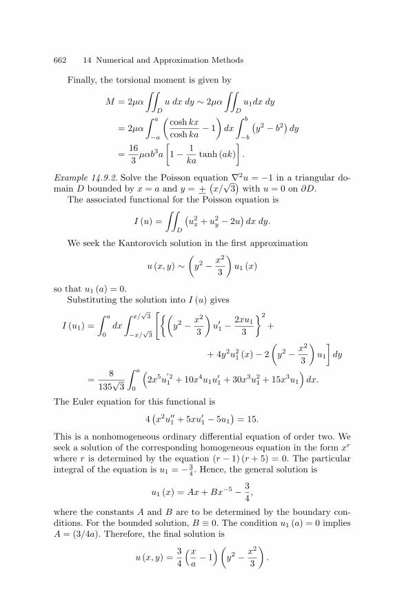
662 14 Numerical and Approximation Methods
Finally, the torsional moment is given by
M = 2µα
∫∫D
u dx dy ∼ 2µα
∫∫D
u1dx dy
= 2µα
∫ a
−a
(cosh kx
cosh ka− 1
)dx
∫ b
−b
(y2 − b2) dy
=163
µαb3a
[1 − 1
katanh (ak)
].
Example 14.9.2. Solve the Poisson equation ∇2u = −1 in a triangular do-main D bounded by x = a and y = +
(x/
√3)
with u = 0 on ∂D.The associated functional for the Poisson equation is
I (u) =∫∫
D
(u2
x + u2y − 2u
)dx dy.
We seek the Kantorovich solution in the first approximation
u (x, y) ∼(
y2 − x2
3
)u1 (x)
so that u1 (a) = 0.Substituting the solution into I (u) gives
I (u1) =∫ a
0dx
∫ x/√
3
−x/√
3
[(y2 − x2
3
)u′
1 − 2xu1
3
2
+
+ 4y2u21 (x) − 2
(y2 − x2
3
)u1
]dy
=8
135√
3
∫ a
0
(2x5u
′21 + 10x4u1u
′1 + 30x3u2
1 + 15x3u1
)dx.
The Euler equation for this functional is
4(x2u′′
1 + 5xu′1 − 5u1
)= 15.
This is a nonhomogeneous ordinary differential equation of order two. Weseek a solution of the corresponding homogeneous equation in the form xr
where r is determined by the equation (r − 1) (r + 5) = 0. The particularintegral of the equation is u1 = − 3
4 . Hence, the general solution is
u1 (x) = Ax + Bx−5 − 34,
where the constants A and B are to be determined by the boundary con-ditions. For the bounded solution, B ≡ 0. The condition u1 (a) = 0 impliesA = (3/4a). Therefore, the final solution is
u (x, y) =34
(x
a− 1
)(y2 − x2
3
).

14.10 The Finite Element Method 663
14.10 The Finite Element Method
Many problems in mathematics, science and engineering are not simpleand cannot be solved by exact closed-form analytical formulas. It is oftennecessary to obtain approximate numerical or asymptotic solutions ratherthan exact solutions. Many numerical methods that have evolved over theyears reduce algebraic or differential equations to discrete form which canbe solved easily by computer. However, if the numerical method is not care-fully chosen, the numerically computed solution may not be anywhere closeto the true solution. Another problem is that the computation for a difficultproblem may take so long that it is impractical for a computer to carry out.The most commonly used numerical methods are finite differences that givepointwise approximations of the governing equations. These methods canbe used successfully to solve many fairly difficult problems, but their majorweakness is that they are not suitable for problems with irregular geome-tries, curved boundaries or unusual boundary conditions. For example, thefinite difference methods are not particularly effective for a circular domainbecause a circle cannot be accurately partitioned into rectangles. However,there are other numerical methods including the finite element method andthe boundary element method.
Unlike finite difference methods, the finite element method can be usedeffectively to determine fairly accurate approximate solutions to a widevariety of governing equations defined over irregular regions. The entire so-lution domain can be modeled analytically or approximated by replacing itwith small, interconnected discrete finite elements (hence the name finiteelement). The solution is then approximated by extremely simple functions(linear functions) on these small elements such as triangles. These small ele-ments are collected together and requirements of continuity and equilibriumare satisfied between neighboring elements.
In a nutshell, the basic idea of the finite element method (FEM) con-sists of decomposing a given domain into a set of finite elements of arbitraryshape and size. This decomposition is usually called a mesh or a grid withthe restriction that elements cannot overlap nor leave any part of the do-main uncovered. For each element, a certain number of points is introducedthat can be located on the edges of the elements or inside. These points arecalled nodes that are usually vertices of triangles as shown in Figure 14.10.1.Finally, these nodes are used to approximate a function under considerationover the whole domain by interpolation in the finite elements.
Historically, the finite element method was developed originally to studystress fields in complicated aircraft structures in the early 1960s. Subse-quently, it has been extended and widely applied to find approximate solu-tions to a wide variety of problems in mathematics, science, and engineering.It was Richard Courant (1888–1972) who first introduced piecewise contin-uous functions defined over triangular domains in 1943; he then used thesetriangular elements combined with the principle of minimum potential en-

664 14 Numerical and Approximation Methods
ergy to study the St. Venant torsion problem in continuum mechanics. Healso described element properties and finite element equations based on avariational principle. In 1965, the finite element method received an evenbroader interpretation when Zienkiewicz and Cheung (1965) suggested thatit is applicable to all field problems that can be cast in variational form.During the late 1960s and early 1970s, considerable attention has been givento errors, bounds and convergence criteria for finite element approximationsto solutions of various problems in continuum mechanics.
In order to develop the finite element method, we recall the celebratedEuler–Lagrange equation (14.6.12) with u (a) = α and u (b) = β. We dividethe interval a ≤ x ≤ b into n parts by the Rn+1 set: a = x0 < x1 < x2 <. . . < xn = b. Each such subinterval is called an element. In general, thelength of the elements need not be equal, though for simplicity, we assumethat they are equal in length so that h = 1
n (b − a). We set uk = u (xk),k = 0, 1, 2, . . . , n so that u0 (x0) = α and un (xn) = β, while u1, u2, . . .,un−1 are unknown quantities. We next rewrite the functional (14.6.3) as
I (u) =∫ x1
x0
F (x, u, u′) dx +∫ x2
x1
F (x, u, u′) dx + . . . +∫ xn
xn−1
F (x, u, u′) dx.
(14.10.1)
We define a piecewise linear interpolating function L (x) of ui as thefunction which is continuous on [a, b] and whose graph consists of straightline segments joining the consecutive pairs of points (xk, uk), (xk+1, uk+1)for k = 0, 1, 2, . . ., (n − 1), that is,
L (x) = uk +1h
(uk+1 − uk) (x − xk) , xk ≤ x ≤ xk+1, (14.10.2)
where k = 0, 1, 2, . . ., (n − 1).Substituting L for u and L′ for u′ in (14.10.1) and assuming that the
integrals can be computed exactly yields
In−1 = In−1 (u1, u2, . . . , un−1) . (14.10.3)
We next find the minimum of In−1 by solving the system of equations
∂In−1
∂uk= 0, k = 1, 2, . . . , (n − 1) . (14.10.4)
The solution of this system (14.10.4) is then substituted into (14.10.2) toobtain a continuous, piecewise linear approximation for the exact solutionu (x).
Example 14.10.1. (The Dirichlet problem for the Poisson equation in aplane).
We consider the problem

14.10 The Finite Element Method 665
− u = f (x, y) in D, (14.10.5)u = 0 on the boundary ∂D. (14.10.6)
The region D is first triangulated so that it is approximated by a regionDn which is the union of a finite number of triangles as shown in Figures14.10.1 (a) and 14.10.1 (b). We denote the interior vertices by V1, V2, . . .,Vn.
We next choose n trial functions v1 (x, y), v2 (x, y), . . ., vn (x, y), one foreach interior vertex. Each trial function vm (x, y) is assumed to be equal to1 at its vertices Vm and equal to zero at all other vertices as in shown inFigure 14.10.1 (c).
Each linear trial function vm (x, y) = ax + by + c, where a, b, and care different for each trial function and for each triangle. This requirementdetermines vm (x, y) uniquely. Indeed, its graph is simply a pyramid of unitheight with its peak at Vm and it is zero on all the triangles which do nottouch Vm.
We next approximate the solution u (x, y) by a linear combination ofthe vm (x, y) so that
un (x, y) = a1v1 (x, y) + a2v2 (x, y) + . . . + anvn (x, y) =n∑
m=1
amvm (x, y) ,
(14.10.7)
where the coefficients a1, a2, . . ., an are to be determined.We multiply the Poisson equation (14.10.5) by any function v (x, y)
which is zero on ∂D and next use Green’s first identity to obtain∫∫D
∇u · ∇v dx dy =∫∫
D
f v dx dy. (14.10.8)
We assume that (14.10.8) is valid only for the first n trial functions sothat v = vk for k = 1, 2, . . ., n. With u (x, y) = un (x, y) and v (x, y) =vk (x, y), result (14.10.8) becomes
Figure 14.10.1 (a), (b), and (c). Triangular elements.

666 14 Numerical and Approximation Methods
n∑m=1
am
[∫∫D
(∇um · ∇vk) dx dy
]=
∫∫D
f vk dx dy. (14.10.9)
This is a system of n linear equations, where m = 1, 2, . . ., n in the nunknown coefficients am, and can be rewritten in the form
n∑m=1
αmk am = fk, k = 1, 2, . . . , n, (14.10.10)
where
αmk =∫∫
D
(∇um · ∇vk) dx dy, fk =∫∫
D
f vk dx dy. (14.10.11)
Consequently, the finite element method leads to finding αmk and fk from(14.10.11) and then solving (14.10.10). Finally, the approximate value ofthe solution u (x, y) is then given by (14.10.7).
Several comments are in order. First, the trial functions vm (x, y) dependon the geometry of the problem and are completely known. Second, theapproximate solution un (x, y) vanishes on the boundary ∂Dn. Third, at avertex Vi = (xi, yi),
un (xi, yi) = aivi (xi, yi) + . . . + anvn (xi, yi) =n∑
r=1
arvr (xi, yi) = ai
where
vr (xk, yk) =
⎧⎨⎩0, r = k
1, r = k.
Fourth, the coefficients ai are exactly the values of the approximate solutionat the vertices Vi = (xi, yi).
Example 14.10.2. We consider the variational problem of finding the ex-tremes of the functional
I (u) =∫ 6
0
(u′2 + u2 − 2u − 2xu
)dx (14.10.12)
with the boundary conditions u (0) = 1 and u (6) = 7.We divide 0 ≤ x ≤ 6 into three equal parts of length h = 2 by x0 = 0,
x1 = 2, x2 = 4 and x3 = 6. We set uk = u (xk) so that u0 = u (0) = 1 andu3 = u (6) = 7, while u1 and u2 are unknown quantities. We have
F (x, u, u′) = u′2 + u2 − 2u − 2xu (14.10.13)
so that

14.10 The Finite Element Method 667
I =∫ 2
0F (x, u, u′) dx +
∫ 4
2F (x, u, u′) dx +
∫ 6
4F (x, u, u′) dx. (14.10.14)
We take
L (x) =
⎧⎪⎪⎪⎪⎨⎪⎪⎪⎪⎩u0 + 1
2 (u1 − u0) x, 0 ≤ x ≤ 2
u1 + 12 (u2 − u1) (x − 2) , 2 ≤ x ≤ 4
u2 + 12 (u3 − u1) (x − 4) , 4 ≤ x ≤ 6,
, (14.10.15)
so that its derivative is
L′ (x) =
⎧⎪⎪⎪⎪⎨⎪⎪⎪⎪⎩
12 (u1 − u0) , 0 ≤ x ≤ 2
12 (u2 − u1) , 2 < x ≤ 4
12 (u3 − u1) , 4 < x ≤ 6.
(14.10.16)
Substituting (14.10.15)–(14.10.16) into (14.10.14) and using (14.10.13) weget
I =∫ 2
0
[(u1 − u0
2
)2
+
u0 +12
(u1 − u0) x
2
− 2
u0 +12
(u1 − u0) x
−2x
u0 +
12
(u1 − u0) x
]dx
+∫ 4
2
[(u2 − u1
2
)2
+
u1 +12
(u2 − u1) (x − 2)2
−2
u1 +12
(u2 − u1) (x − 2)
− 2x
u1 +
12
(u2 − u1) (x − 2)]
dx
+∫ 6
4
[(u3 − u1
2
)2
+
u2 +12
(u3 − u1) (x − 4)2
−2
u2 +12
(u3 − u1) (x − 4)
−2x
u2 +
12
(u3 − u1) (x − 4)]
dx.
Using the known values of u0 and u3 and integrating we obtain (n = 3)
I2 =73(u2
1 + u22) − 1
3u1u2 − 37
3u1 − 67
3u2 − 101
3.
Consequently, equation (14.10.4) gives two equations
∂I2
∂u1=
143
u1 − 13
u2 − 373
= 0,
∂I2
∂u2= −1
3u1 +
143
u2 − 673
= 0.

668 14 Numerical and Approximation Methods
Thus, the solutions for u1 and u2 are u1 = 3 and u2 = 5.Putting these values into (14.10.15) leads to the approximate solution
L (x) = 1 + x, 0 ≤ x ≤ 6. (14.10.17)
In this problem, the Euler–Lagrange equation for (14.10.12) is given by
u′′ − u = − (1 + x) . (14.10.18)
Solving this equation with u (0) = 1 and u (6) = 7 yields the exact solution
u (x) = 1 + x.
In this example, the exact and approximate solutions are identical dueto the simplicity of the problem. In general, these solutions will be different.
We close this section by adding some comments on another numericaltechnique known as the boundary element method (boundary integral equa-tion method). This method was widely used in early research in solid me-chanics, fluid mechanics, potential theory and electromagnetic theory. How-ever, the major breakthrough in the boundary integral equation methodcame in 1963 when two classic papers were published by Jaswon (1963) andSymm (1963). The boundary element method is based on the mathemati-cal aspect of finding the Green’s function solution of differential equationswith prescribed boundary conditions. It also uses Green’s theorem to re-duce a volume problem to a surface problem, and a surface problem to aline problem. This technique is not only very useful but also very accuratefor linear problems, especially for three dimensional problems with rapidlychanging variables in fracture and contact problems in solid mechanics.However, this method is computationally less efficient than the finite ele-ment method, and is not widely used in industry. It is fairly popular forfinding numerical solutions of acoustic problems. Since the early 1970s theboundary element method has continued to develop at a fast pace and hasbeen extended to include a wide variety of linear and nonlinear problemsin continuum mechanics.
14.11 Exercises
1. Obtain the explicit finite difference solution of the problem
utt − 4uxx = 0, 0 < x < 1, t > 0,
u (0, t) = u (1, t) = 0, t ≥ 0,
u (x, 0) = sin 2πx, ut (x, 0) = 0, 0 ≤ x ≤ 1.
Compare the numerical solution with the analytical solution
u (x, t) = cos 4πt sin 2πx
at several points.

14.11 Exercises 669
2. (a) Calculate an explicit finite difference solution of the wave equation
uxx − utt = 0, 0 < x < 1, t > 0,
satisfying the boundary conditions
u (0, t) = u (1, t) = 0, t ≥ 0,
and the initial conditions
u (x, 0) =18
sin πx, ut (x, 0) = 0, 0 ≤ x ≤ 1.
Show that the exact solution of the problem is
u (x, t) =18
cos πt sin πx.
Compare the two solutions at several points.(b) Solve the wave equation in (a) with the same boundary data andthe initial data
u (x, 0) = sinπx, ut (x, 0) = 0, 0 ≤ x ≤ 1.
3. Use the Lax–Wendroff method to find a numerical solution of the prob-lem
ux + ut = 0, x > 0, t > 0,
u (x, 0) = 2 + x, x > 0,
u (0, t) = 2 − t, t > 0.
Show that the exact solution of the problem is
u (x, t) = 2 + (x − t) .
Compare the two solutions at various points.
4. Show that the finite difference approximation to the equation
aut + bux = f (x, t)
is
ui,j+1 − 12
(ui+1,j + ui−1,j) +(
εb
2a
)(ui+1,j − ui−1,j) − fi,j = 0,
where a, b are constants and ε = k/h.

670 14 Numerical and Approximation Methods
5. Obtain a finite difference solution of the heat conduction problem
ut = κuxx, 0 < x < l, t > 0,
with the boundary conditions
u (0, t) = u (l, t) = 0, t > 0,
and the initial condition
u (x, 0) =4x
l(l − x) , 0 ≤ x ≤ l.
6. (a) Find an explicit finite difference solution of the parabolic system
ut = uxx, 0 < x < 1, t > 0,
u (0, t) = u (1, t) = 0, t > 0,
u (0, t) = sinxπ on 0 ≤ x ≤ 1.
Compare the numerical results with the analytical solution
u (x, t) = e−π2t sin πx,
at t = 0.5 and t = 0.05.(b) Prove that the Richardson finite difference scheme for problem 6(a)is
ui,j+1 = ui,j−1 + 2 ε δ2x ui,j .
Hence, show that the exact solution of this equation is
ui,j =(A1α
j1 + A2α
j2
)sin πhi,
where α1 and α2 are the roots of the quadratic equation
x2 + 8εx sin2 (πh/2) − 1 = 0.
7. Using four internal grid points, find the explicit finite difference solutionof the Dirichlet problem
∇2u ≡ uxx + uyy = 0, 0 < x < 1, 0 < y < 1,
u (x, 0) = x (1 − x) , u (x, 1) = 0 on 0 ≤ x ≤ 1,
u (0, y) = u (1, y) = 0, on 0 ≤ y ≤ 1.
Compare the numerical solution with the exact analytical solution
u (x, y) =4π3
∞∑n=0
2(2n + 1)3
sin nπx sinhnπ (1 − y)sinhnπ
at the point (x, y) =( 1
3 , 13
).

14.11 Exercises 671
8. Solve the Dirichlet problem by the explicit finite difference method
uxx + uyy = 0, 0 < x < 1, 0 < y < 1,
u (x, 0) = sinπx, u (x, 1) = 0 on 0 ≤ x ≤ 1,
u (x, y) = 0, for x = 0, x = 1 and 0 ≤ y ≤ 1.
9. Using a square grid system with h = 12 , find the finite difference solution
of the Laplace equation on the quarter-disk given by
uxx + uyy = 0, x2 + y2 < 1, y > 0,
u (x, 0) = 0, −1 < x < 1,
u (x, y) = 102, x2 + y2 = 1, y > 0.
10. Find a finite difference solution of the wave problem
utt − uxx = 0, 0 < x < 1, t > 0,
u (0, t) = u (1, t) = 0, t ≥ 0,
u (x, 0) =12
x (1 − x) , ut (x, 0) = 0, 0 ≤ x ≤ 1.
Compare the numerical results with the exact analytical solution
u (x, t) =2π3
∞∑r=1
1r3 1 − (−1)r cos πrt sin πrx,
at various points.
11. Obtain a finite difference solution of the problem
utt = c2uxx, 0 < x < 1, t > 0,
u (0, t) = sinπct, u (1, t) = 0, t ≥ 0,
u (x, 0) = ut (x, 0) = 0, 0 ≤ x ≤ 1.
12. Show that the transformation v = log u transforms the nonlinear system
vt = vxx + v2x, 0 < x < 1, t > 0,
vx (0, t) = 1, v (1, t) = 0, t ≥ 0,
v (x, 0) = 0, 0 ≤ x ≤ 1
into the linear system
ut = uxx, 0 < x < 1, t > 0,
ux (0, t) = u (0, t) , u (x, 1) = 1, t ≥ 0,
u (x, 0) = 1, 0 ≤ x ≤ 1.
Solve the linear system by the explicit finite difference method with thederivative boundary condition approximated by the central differenceformula.

672 14 Numerical and Approximation Methods
13. Solve the following parabolic system by the Crank–Nicolson method
ut = uxx, 0 < x < 1, t > 0,
u (0, t) = u (1, t) = 0, t ≥ 0,
with the initial condition
(a) u (x, 0) = 1, 0 ≤ x ≤ 1,
(b) u (x, 0) = sinπx, 0 ≤ x ≤ 1.
(c) u (x, 0) = sinπx, 0 ≤ x ≤ 1
with 0 ≤ t ≤ 0.2 and in formula (14.5.2) κ = 1, k = h2.
14. Use the Crank–Nicolson implicit method with the central differenceformula for the boundary conditions to find a numerical solution of thedifferential system
ut = uxx, 0 < x < 1, t > 0,
ux (0, t) = ux (1, t) = −u, t ≥ 0,
u (x, 0) = 1, 0 ≤ x ≤ 1.
15. Find a numerical solution of the wave equation
utt = c2uxx, 0 < x < l, t > 0,
with the boundary and initial conditions
u =120
ux at x = 0 and x = l, t > 0,
u (x, 0) = 0, ut (x, 0) = a sin(πx
l
)0 ≤ x ≤ l.
16. Determine the function representing a curve which makes the followingfunctional extremum:
(a) I (y (x)) =∫ 1
0
(y′2 + 12xy
)dx, y (0) = 0, y (1) = 1,
(b) I (y (x)) =∫ π/2
0
(y′2 − y2) dx, y (0) = 0, y
(π
2
)= 1,
(c) I (y (x)) =∫ x1
x0
1x
(1 + y′2) 1
2 dx.
17. In the problem of tautochroneous motion, find the equation of the curvejoining the origin O and a point A in the vertical (x, y)-plane so that aparticle sliding freely from A to O under the action of gravity reachesthe origin O in the shortest time, friction and resistance of the mediumbeing neglected.

14.11 Exercises 673
18. In the problem of minimum surface of revolution, determine a curvewith given boundary points (x0, y0) and (x1, y1) such that rotation ofthe curve about the x-axis generates a surface of revolution of minimumarea.
19. Show that the Euler equation of the variational principle
δI [u (x, y)] = δ
∫∫D
F (x, y, u, p, q, l, m, n) dx dy = 0
is
Fu − ∂
∂xFp − ∂
∂yFq +
∂2
∂x2 Fl +∂2
∂x∂yFm +
∂2
∂y2 Fn = 0,
where
p = ux, q = uy, l = uxx, m = uxy, n = uyy.
20. Prove that the Euler–Lagrange equation for the functional
I =∫∫∫
R
F (x, y, z, u, p, q, r, l, m, n, a, b, c) dx dy dz
is
Fu − ∂
∂xFp − ∂
∂yFq +
∂2
∂zFr +
∂2
∂x2 Fl +∂2
∂y2 Fm
+∂2
∂z2 Fn +∂2
∂x∂yFa +
∂2
∂y∂zFb +
∂2
∂z∂xFc = 0,
where (p, q, r) = (ux, uy, uz), (l, m, n) = (uxx, uyy, uzz), and (a, b, c) =(uxy, uyz, uzx).
21. In each of the following cases apply the variational principle or its sim-ple extension with appropriate boundary conditions to derive the cor-responding equations:
(a) F = u2x + u2
y + 2u2xy.
(b) F = 12
[u2
t − α(u2
x + u2y
) − β2u2],
(c) F = 12
(utux + αu2
x − βu2xx
),
(d) F = 12
(u2
t − α2u2xx
),
(e) F = p (x) u′2 + ddx
(q (x) u2
) − [r (x) + λs (x)] u2,
where p, q, r, and s are given functions of x, and α, β are constants.

674 14 Numerical and Approximation Methods
22. Derive the Schrodinger equation from the variational principle
δ
∫∫∫R
[
2
2m
(ψ2
x + ψ2y + ψ2
z
)+ (V − E) ψ2
]dx dy dz = 0,
where h = 2π is the Planck constant, m is the mass of a particle movingunder the action of a force field described by the potential V (x, y, z)and E is the total energy of the particle.
23. Derive the Poisson equation ∇2u = F (x, y) from the variational prin-ciple with the functional
I (u) =∫∫
D
[u2
x + u2y + 2uF (x, y)
]dx dy,
where u = u (x, y) is given on the boundary ∂D of D.
24. Derive the equation of motion of a vibrating string of length l underthe action of an external force F (x, t) from the variational principle
δ
∫ t2
t1
∫ l
0
[(12
ρ u2t − T ∗u2
x
)+ ρ uF (x, t)
]dx dt = 0,
where ρ is the line density and T ∗ is the constant tension of the string.
25. The kinetic and potential energies associated with the transverse vibra-tion of a thin elastic plate of constant thickness h are
T =12
ρ
∫∫D
u2dx dy,
V =12
µ0
∫∫D
[(∇u)2 − 2 (1 − σ)
(uxxuyy − u2
xy
)]dx dy,
where ρ is the surface density and µ0 = 2h3E/3(1 − σ2
).
Use the variational principle
δ
∫ t2
t1
∫∫D
[(T − V ) + fu] dx dy dt = 0
to derive the equation of motion of the plate
ρu + µ0∇4u = f (x, y, t) ,
where f is the transverse force per unit area acting on the plate.
26. The kinetic and potential energies associated with the wave motion inelastic solids are

14.11 Exercises 675
T =12
∫∫∫D
ρ(u2
t + v2t + w2
t
)dx dy dz
V =12
∫∫∫D
[λ (ux + vy + wz)
2 + 2µ(u2
x + v2y + w2
z
)+µ
(vx + uy)2 + (wy + vz)
2 + (uz + wx)2]
dx dy dz.
Use the variational principle
δ
∫ t2
t1
∫∫∫D
(T − V ) dx dy dz = 0
to derive the equation of wave motion in an elastic medium
(λ + µ) grad divu + µ∇2u = ρutt,
where u = (u, v, w) is the displacement vector.
27. From the variational principle
δ
∫∫D
L dx dt = 0 with L = −ρ
∫ η
−h
φt +
12
(∇φ)2 + gz
dz
derive the basic equations of water waves
∇2φ = 0, −h (x, y) < z < η (x, y, t) , t > 0,
ηt + ∇φ · ∇η − φz = 0, on z = η,
φz +12
(∇φ)2 + gz = 0, on z = η,
φz = 0, on z = −h,
where φ (x, y, z, t) is the velocity potential, and η (x, y, t) is the freesurface displacement function in a fluid of depth h.
28. Derive the Boussinesq equation for water waves
utt − c2uxx − µ uxxtt =12(u2)
xx
from the variational principle
δ
∫∫L dx dt = 0,
where L ≡ 12 φ2
t − 12 c2 φ2
x + 12µ φ2
xt − 16φ3
x and φ is the potential foru (u = φx).
29. Determine an approximate solution of the problem of finding an ex-tremum of the functional
I (y (x)) =∫ 1
0
(y′2 − y2 − 2xy
)dx, y (0) = y (1) = 0.

676 14 Numerical and Approximation Methods
30. Find an approximate solution of the torsion problem of a cylinder withan elliptic base; the domain of integration D is the interior of the ellipsewith the major and minor axes 2a and 2b respectively. The associatedfunctional is
I (u (x, y)) =∫∫
D
[(∂u
∂x− y
)2
u +(
∂u
∂y+ x
)2
u
]dx dy.
31. Use the Rayleigh–Ritz method to find an approximate solution of theproblem
∇2u = 0, 0 < x < 1, 0 < y < 1,
u (0, y) = 0 = u (1, y) ,
u (x, 0) = x (1 − x) .
32. Find an approximate solution of the boundary-value problem
∇2u = 0, x > 0, y > 0, x + 2y < 2,
u (0, y) = 0, u (x, 0) = x (2 − x) ,
u (2 − 2y, y) = 0.
33. In the torsion problem in elasticity, the Prandtl stress functionΨ (x, y) = ψ (x, y) − 1
2
(x2 + y2
)satisfies the boundary value problem
∇2Ψ = −2 in D
Ψ = 0 on ∂D.
Use the Galerkin method to find an approximate solution of the problemin a rectangular domain D = (x, y) : −a ≤ x ≤ a,−b ≤ y ≤ b.
34. Apply the Galerkin approximation method to find the first eigenvalueof the problem of a circular membrane of radius a governed by theequation
∇2u ≡ d2u
dr2 +1r
du
dr= λu in 0 < r < a
u = 0, on r = a.
35. Use the Rayleigh–Ritz method to find the solution in the first approxi-mation of the problem of deformation of an elastic plate (−a ≤ x ≤ a ,−a ≤ y ≤ a) by a parabolic distribution of tensile forces over its op-posite sides at x = + a. The problem is governed by the differentialsystem
∇4u =2α
a2 in |x| < a and |y| < a,(u,
∂u
∂x
)= (0, 0) on |x| = a,(
u,∂u
∂y
)= (0, 0) on |y| = a,

14.11 Exercises 677
where U = u0 + u = 12αy2
(1 − 1
6y2)
+ u, and ∇4U = 0.
36. Show that the Kantorovich solution of the torsion problem in exercise33 is
Ψ1 (x, y) =12(b2 − y2)(
1 − cosh kx
cosh ka
), k =
1b
√52.
37. (a) If the functional I in (14.6.3) depends on two functions u and v,that is,
I (u, v) =∫ b
a
F (x, u, v, u′, v′) dx,
show that there are two Euler–Lagrange equations for this functional
∂F
∂u− d
dx
(∂F
∂u′
)= 0, and
∂F
∂v− d
dx
(∂F
∂v′
)= 0.
(b) Generalize the above result for the functional
I (u) =∫ b
a
F (x,u,u′) dx,
where u = (u1, u2, . . . , un), ui ∈ C2 ([a, b]), and ui (a) = ai and ui (b) =bi, i = 1, 2, . . ., n.
38. Show that the Euler–Lagrange equation for the functional
I [u (x, y)] =∫∫
D
(1 + u2
x + u2y
) 12 dx dy
is (1 + u2
y
)uxx − 2ux uy uxy +
(1 + u2
x
)uyy = 0.
39. Show that the Euler–Lagrange equation for the functional
I (u) =∫∫
D
F (x, y, u, ux, uy, uxx, uxy, uyy) dx dy
is
∂F
∂u− ∂
∂x(Fux) − ∂
∂y
(Fuy
)+
∂2
∂x2 (Fuxx) +∂2
∂x∂y
(Fuxy
)+
∂2
∂y2
(Fuyy
)= 0.

678 14 Numerical and Approximation Methods
40. Derive the Euler–Lagrange equation for the functional
I [y (x)] =∫ b
a
F (x, y, y′) dx
where
(a) F (x, y, y′) = u (x, y)√
1 + y′2,
(b) F (x, y, y′) = 1√2g
(1+y′2
y1−y
) 12
with y (a) = y1 and y (b) = y2 < y1, (Brachistochrone problem).
(c) F (x, y, y′) = y′2 (1 + y′2)2,
(d) F (x, y, y′) =(xy3 − y′2 + 3xyy′).
41. Show that there are an infinite number of continuous functions withpiecewise continuous first derivatives that minimize the functional
I [y (x)] =∫ 2
0y′2 (1 + y′)2 dx
with y (0) = 1 and y (2) = 0.
42. The torsion of a prismatic rod of rectangular cross section of length 2aand width 2b is governed by
∇2u = 2 in R = (x, y) : −a < x < a, −b < y < bu = 0 on ∂R.
(a) Find an approximate solution u1 (x, y). Hence, calculate the tor-sional moment M for a = b and for a = b.
(b) Find the exact classical solution for u (x, y) and the torsional mo-ment M .
43. Find an approximate solution of the biharmonic problem
∇4u = 0, R = (x, y) : −a < x < a, −b < y < bwith the boundary conditions
uxy = 0, uyy = c
(1 − y2
b2
)for x = + a,
uxy = 0, uxx = 0 for y = + b,
where c is a constant.

14.11 Exercises 679
44. Show that the Euler–Lagrange equation (14.6.12) can be written in theform
d
dx
(F − u′ ∂F
∂u′
)− ∂F
∂x= 0.
45. Show that the extremals of the functional
I [y (x)] =∫ b
a
[p (x) y′2 − q (x) y2] dx
subject to the constraint
J [y (x)] =∫ b
a
r (x) y2dx = 1,
are solutions of the Sturm–Liouville equation
d
dx
[p (x)
dy
dx
]+ [q (x) + λ r (x)] y = 0.
46. Consider the finite element method for the wave equation
utt − uxx = 0, 0 ≤ x ≤ l, t > 0,
u (0) = u (l) = 0,
with given initial conditions.
(a) Show that an appropriate requirement is that
n∑i=1
A′′i (t)
∫ l
0vi (x) vj (x) dx +
n∑i=1
Ai (t)∫ l
0
∂vi
∂x· ∂vj
∂xdx = 0,
where j = 1, 2, . . ., n and that the approximate solution is given by
un (x) = A1 (t) v1 (x) + . . . + An (t) vn (t) =n∑
i=1
Ai (t) vi (x) .
(b) Show that the finite element method leads to a system of ordinarydifferential equations
Bd2A
dt2+ C A (t) = 0, A (0) = D
where B and C are n × n matrices, A (t) is a n-vector function and Dis an n-vector.

15
Tables of Integral Transforms
In this chapter we provide a set of short tables of integral transforms of thefunctions that are either cited in the text or are in most common use inmathematical, physical, and engineering applications. For exhaustive lists ofintegral transforms, the reader is referred to Erdelyi et al. (1954), Campbelland Foster (1948), Ditkin and Prudnikov (1965), Doetsch (1970), Marichev(1983), Debnath (1995), and Oberhettinger (1972).
15.1 Fourier Transforms
f (x) F (k) = 1√2π
∫ ∞
−∞exp (−ikx) f (x) dx
1 exp (−a |x|) , a > 0(√
2π
)a(a2 + k2
)−1
2 x exp (−a |x|) , a > 0(√
2π
)(−2aik)
(a2 + k2
)−2
3 exp(−ax2
), a > 0 1√
2aexp
(−k2
4a
)
4(x2 + a2
)−1, a > 0
√π2
exp(−a|k|)a
5 x(x2 + a2
)−1 √π2
(ik2a
)exp (−a |k|)

682 15 Tables of Integral Transforms
f (x) F (k) = 1√2π
∫ ∞
−∞exp (−ikx) f (x) dx
6
c, a ≤ x ≤ b0, outside.
ic√2π
1k
(e−ibk − e−iak
)
7 |x| exp (−a |x|) , a > 0√
2π
(a2 − k2
) (a2 + k2
)−2
8 sin axx
√π2 H (a − |k|)
9 exp −x (a − iω) H (x) 1√2π
i(ω−k+ia)
10(a2 − x2
)− 12 H (a − |x|) √
π2 J0 (ak)
11sin
[b(x2+a2)
12
]
(x2+a2)12
√π2 J0
(a√
b2 − k2)H (b − |k|)
12cos(b
√a2−x2)
(a2−x2)12
H (a − |x|) √π2 J0
(a√
b2 + k2)
13 e−ax H (x) , a > 0 1√2π
(a − ik)(a2 + k2
)−1
14 1√|x| exp (−a |x|) , a > 0
(a2 + k2
)− 12[a +
(a2 + k2
) 12] 1
2
15 δ(n) (x − a) , n = 0, 1, 2, . . . 1√2π
(ik)n exp (−iak)
16 exp (iax)√
2π δ (k − a)

15.2 Fourier Sine Transforms 683
15.2 Fourier Sine Transforms
f (x) Fs (k) =√
2π
∫ ∞
0sin (kx) f (x) dx
1 exp (−ax) , a > 0√
2π k
(a2 + k2
)−1
2 x exp (−ax) , a > 0√
2π (2ak)
(a2 + k2
)−2
3 xα−1, 0 < α < 1√
2π k−αΓ (α) sin
(πα2
)
4 1√x
1√k, k > 0
5 xα−1e−ax, α > −1,a > 0
√2π Γ (α) r−α sin (αθ) , where
r =(a2 + k2
) 12 , θ = tan−1
(ka
)
6 x−1e−ax, a > 0√
2π tan−1
(ka
), k > 0
7 x exp(−a2x2
)2−3/2
(ka3
)exp
(− k2
4a2
)
8 erfc (ax)√
2π
1k
[1 − exp
(− k2
4a2
)]
9 x(a2 + x2
)−1 √π2 exp (−ak) , a > 0
10 x(a2 + x2
)−2 1√2π
(ka
)exp (−ak) , (a > 0)

684 15 Tables of Integral Transforms
f (x) Fs (k) =√
2π
∫ ∞
0sin (kx) f (x) dx
11 H (a − x) , a > 0√
2π
1k (1 − cos ak)
12 x−1J0 (ax)
⎧⎪⎨⎪⎩√
2π sin−1 (
ka
), 0 < k < a
√π2 , a < k < ∞
13 x(a2 + x2
)−1J0 (bx) ,
a > 0, b > 0
√π2 e−akI0 (ab) , a < k < ∞
14 J0 (a√
x) , a > 0√
2π
1k cos
(a2
4k
)
15(x2 − a2
)ν− 12 H (x − a) ,
|ν| < 12
2ν− 12(
ak
)νΓ
(ν + 1
2
)J−ν (ak)
16 x1−ν(x2 + a2
)−1Jν (ax) ,
ν > − 32 , a, b > 0
√π2 a−ν exp (−ak) Iν (ab) ,
a < k < ∞
17 x−νJν+1 (ax) , ν > − 12
k(a2−k2)ν− 12
2ν− 12 aν+1Γ(ν+ 1
2 )H (a − k)
18 erfc (ax)√
2π
1k
[1 − exp
(− k2
4a2
)]
19 x−α, 0 < Re α < 2√
2π Γ (1 − α) kα−1 cos
(απ2
)
20(ax − x2
)α− 12 H (a − x),
α > − 12
√2 Γ
(α + 1
2
) (ak
)α sin(
ak2
)Jα
(ak2
)

15.3 Fourier Cosine Transforms 685
15.3 Fourier Cosine Transforms
f (x) Fc (k) =√
2π
∫ ∞
0cos (kx) f (x) dx
1 exp (−ax) , a > 0(√
2π
)a(a2 + k2
)−1
2 x exp (−ax) , a > 0(√
2π
) (a2 − k2
) (a2 + k2
)−2
3 exp(−a2x2
) 1a√
2exp
(− k2
4a2
)
4 H (a − x)√
2π
( sin akk
)
5 xa−1, 0 < a < 1√
2π Γ (a) k−a cos
(aπ2
)
6 cos(ax2
), a > 0 1
2√
a
[cos
(k2
4a
)+ sin
(k2
4a
)]
7 sin(ax2
), a > 0 1
2√
a
[cos
(k2
4a
)− sin
(k2
4a
)]
8(a2 − x2
)ν− 12 H (a − x) , ν > − 1
2 2ν− 12 Γ
(ν + 1
2
) (ak
)νJν (ak)
9(a2 + x2
)−1J0 (bx) , a, b > 0
√π2 a−1 exp (−ak) I0 (ab),
b < k < ∞
10 x−νJν (ax) , ν > − 12
(a2−k2)ν− 12 H(a−k)
2ν− 12 aνΓ(ν+ 1
2 )

686 15 Tables of Integral Transforms
f (x) Fc (k) =√
2π
∫ ∞
0cos (kx) f (x) dx
11(x2 + a2
)− 12 exp
[−b
(x2 + a2
) 12]
K0
[a(k2 + b2
) 12], a > 0, b > 0
12 xν−1e−ax, ν > 0, a > 0√
2π Γ (ν) r−ν cos nθ, where
r =(a2 + k2
) 12 , θ = tan−1
(ka
)
13 2x e−x sin x
√2π tan−1
( 2k2
)
14 sin[a(b2 − x2
) 12 H (b − x)
] √π2 (ab)
(a2 + k2
)− 12
× J1
[b(a2 + k2
) 12]
15 (1−x2)(1+x2)2
√π2 k exp (−k)
16 x−α, 0 < α < 1√
π2
kα−1
Γ (α) sec(
πα2
)
17( 1
a + x)e−ax, a > 0
√π2
2a2
(a2+k2)2
18 log(1 + a2
x2
), a > 0
√2π
(1−e−ak)k
19 log(
a2+x2
b2+x2
), a, b > 0
√2π
(e−bk−e−ak)k
20 a(x2 + a2
)−1, a > 0
√π2 exp (−ak) , k > 0

15.4 Laplace Transforms 687
15.4 Laplace Transforms
f (t) f (s) =∫ ∞
0exp (−st) f (t) dt
1 f (n) (t) snf (s) −n−1∑r=0
sn−r−1f (r) (0)
2∫ t
0f (t − τ) g (τ) dτ f (s) g (s)
3 tnf (t) (−1)n dn
dsn f (s)
4 f (t − a) H (t − a) exp (−as) f (s)
5 tn (n = 0, 1, 2, 3, . . .) n!sn+1
6 eat 1s−a
7 tne−at Γ (n+1)(s+a)n+1
8 ta (a > −1) Γ (a+1)sa+1
9 eat cos bt s−a(s−a)2+b2
10 eat sin bt b(s−a)2+b2
11 1√t
√πs
12 2√
t 1s
√πs

688 15 Tables of Integral Transforms
f (t) f (s) =∫ ∞
0exp (−st) f (t) dt
13 t−1/2 exp(−a
t
) √πs exp (−2
√as)
14 t−3/2 exp(−a
t
) √πa exp (−2
√as)
15 1√πt
(1 + 2at) eat s(s−a)
√s−a
16 12√
πt3
(ebt − eat
) √s − a − √
s − b
17 exp(a2t
)erf
(a√
t)
a√s(s−a2)
18 exp(a2t
)erfc
(a√
t) 1√
s(√s+a)
19 1√πt
+ a exp(a2t
)erf
(a√
t) √
s(s−a2)
20 1√πt
− a exp(a2t
)erfc
(a√
t) 1√
s+a
21 exp(−at)√b−a
erf(√
(b − a) t)
1(s+a)
√s+b
2212eiωt
[exp (−λz) erfc
(ζ −
√iωt
)+ exp (λz) erfc
(ζ +
√iωt
)],
where ζ = z/2√
νt, λ =√
iων
(s − iω)−1 exp(−z
√sν
)
23 12
[exp (−ab) erfc
(b−2at2√
t
)+ exp (ab) erfc
(b+2at2√
t
)] exp[−b
(s + a2
) 12]

15.4 Laplace Transforms 689
f (t) f (s) =∫ ∞
0exp (−st) f (t) dt
24 J0 (at)(s2 + a2
)− 12
25 I0 (at)(s2 − a2
)− 12
26 tα−1 exp (−at) , α > 0 Γ (α) (s + a)−α
27 t−1Jν (at) ν−1aν(√
s2 + a2 + s)−ν
,Re ν > − 1
2
28 J0(a√
t) 1
s exp(−a2
4s
)
29( 2
a
)νtν/2Jν
(a√
t)
s−(ν+1) exp(−a2
4s
),
Re ν > − 12
30 a2t
√πt
exp(−a2
4t
)exp (−a
√s) , a > 0
31 1√πt
exp(−a2
4t
)1√s
exp (−a√
s) , a ≥ 0
32 exp(−a2t2
4
) √π
a exp(
s2
a2
)erfc
(sa
),
a ≥ 0
33(t2 − a2
)− 12 H (t − a) K0 (as) , a > 0
34 δ(n) (t − a) , n = 0, 1, . . . sn exp (−as)

690 15 Tables of Integral Transforms
f (t) f (s) =∫ ∞
0exp (−st) f (t) dt
35 tmα+β−1E(m)α,β (+ at) ,
m = 0, 1, 2, . . .
m! sα−β
(sα+ a)m+1
36√
π
Γ(ν+ 12 )
(t2a
)νJν (at)
(s2 + a2
)−(ν+ 12 ),
Re ν > − 12
37 12e−ct
[exp
(−a√
b − c)
×erfc
a√4t
− √(b − c) t
− exp
(a√
b − c)
×erfc
a√4t
+√
(b − c) t]
exp(−a√
s+b)(s+c)
√(s+b)
38 12e−ct
[exp
(−a√
b − c)
×erfc
a√4t
− t√
b − c
− exp(a√
b − c)
×erfc
a√4t
+ t√
b − c]
exp(−a√
s+b)(s+c)
39 e−bt[√
4tπ exp
(−a2
4t
)−a erfc
(a√4t
)] exp(−a√
s+b)(s+b)3/2
40 e−bt[(
t + 12a2
)erfc
(a√4t
)−√
ta2
π exp(−a2
4t
)] exp(−a√
s+b)(s+b)2

15.5 Hankel Transforms 691
15.5 Hankel Transforms
f (r) ordern
fn (k) =∫ ∞
0r Jn (kr) f (r) dr
1 H (a − r) 0 akJ1 (ak)
2 exp (−ar) 0 a(a2 + k2
)− 32
3 1r exp (−ar) 0
(a2 + k2
)− 12
4(a2 − r2
)H (a − r) 0 4a
k3 J1 (ak) − 2a2
k2 J0 (ak)
5 a(a2 + r2
)− 32 0 exp (−ak)
6 1r cos (ar) 0
(k2 − a2
)− 12 H (k − a)
7 1r sin (ar) 0
(a2 − k2
)− 12 H (a − k)
8 1r2 (1 − cos ar) 0 cosh−1 (
ak
)H (a − k)
9 1r J1 (ar) 0 1
a H (a − k) , a > 0
10 Y0 (ar) 0( 2
π
) (a2 − k2
)−1
11 K0 (ar) 0(a2 + k2
)−1

692 15 Tables of Integral Transforms
f (r) ordern
fn (k) =∫ ∞
0r Jn (kr) f (r) dr
12 δ(r)r 0 1
13(r2 + b2
)− 12
× exp
−a(r2 + b2
) 12 0
(k2 + a2
)− 12 exp
−b
(k2 + a2
) 12
14(r2 + a2
)− 12 0 1
k exp (−ak)
15 exp (−ar) 1 k(a2 + k2
)−3/2
16 sin arr 1 a H(k−a)
k(k2−a2)12
17 1r exp (−ar) 1 1
k
[1 − a
(k2+a2)12
]
18 1r2 exp (−ar) 1 1
k
[(k2 + a2
) 12 − a
]
19 rn H (a − r) > −1 1k an+1 Jn+1 (ak)
20 rn exp (−ar), (Re a > 0) > −1 1√π
2n+1 Γ(n+ 32 ) a kn
(a2+k2)n+ 32
21 rn exp(−ar2
)> −1 kn
(2a)n+1 exp(−k2
4a
)

15.5 Hankel Transforms 693
f (r) ordern
fn (k) =∫ ∞
0r Jn (kr) f (r) dr
22 ra−1 > −12a Γ [ 1
2 (a+n+1)]ka+1 Γ [ 1
2 (1−a+n)]
23 rn(a2 − r2
)m−n−1
× H (a − r)> −1 2m−n−1 Γ (m − n) amkn−mJm (ak)
24 rm exp(−r2/a2
)> −1 kn am+n+2
2n+1 Γ (n+1) Γ(1 + m
2 + n2
)× 1F1
(1 + m
2 + n2 ; n + 1; − 1
4a2k2)
25 1r Jn+1 (ar) > −1 kna−(n+1)H (a − k), a > 0
26 rn(a2 − r2
)mH (a − r),
m > −1> −1 2manΓ (m + 1)
(ak
)m+1
×Jn+m+1 (ak)
27 1r2 Jn (ar) > 1
2
⎧⎨⎩12n
(ka
)n, 0 < k ≤ a
12n
(ak
)n, a < k < ∞
28 rn
(a2+r2)m+1 , a > 0 > −1(
k2
)m an−m
Γ (m+1) Kn−m (ak)
29 exp(−p2r2
)Jn (ar) > −1
(2p2
)−1 exp(−a2+k2
4p2
)In
(ak2p2
)
30 1r exp (−ar) > −1
[(k2+a2)
12 −a
]n
kn(k2+a2)12
31 rn
(r2+a2)n+1 > −1(
k2
)n K0(ak)Γ (n+1)

694 15 Tables of Integral Transforms
f (r) ordern
fn (k) =∫ ∞
0r Jn (kr) f (r) dr
32 rn
(a2−r2)n+ 12
H (a − r) < 1 1√π
(k2
)nΓ
( 12 − n
) ( sin akk
)
33 f (ar) n 1a2 fn
(ka
)
34 r−1 exp(−ar2
)1 1
k
[1 − exp
(−k2
4a
)]
35 r−1 sin(ar2
), a > 0 1 1
k sin(
k2
4a
)
36 r−1 cos(ar2
), a > 0 1 1 − cos
(k2
4a
)
37 exp (−ar) , a > 0 > −1 (a+n√
k2+a2)(k2+a2)3/2
(k
a+√
a2+k2
)n
38 exp(−ar2
)J0 (br) 0 a
2 exp(−k2−b2
4a
)I0
(bk2a
)
39 H(a−r)√a2−r2 0
√aπ2k J 1
2(ak) , a > 0
40 rnH(a−r)√a2−r2 > −1
√π2k an+ 1
2 Jn+1 (ak) , a > 0
41 r−2 sin r 0 sin−1 ( 1k
), (k > 1)

15.6 Finite Hankel Transforms 695
15.6 Finite Hankel Transforms
f (r) ordern
fn (ki) =∫ a
0r Jn (r ki) f (r) dr
1 c, where c is a constant 0(
acki
)J1 (aki)
2(a2 − r2
)0 4a
k3iJ1 (aki)
3(a2 − r2
)− 12 0 k−1
i sin (aki)
4 J0(αr)J0(αa) 0 − aki
(α2−k2i )
J1 (aki)
5 1r 1 k−1
i 1 − J0 (aki)
6 r−1(a2 − r2
)− 12 1 (1−cos aki)
(aki)
7 rn > −1 an+1
kiJn+1 (aki)
8 Jν(αr)Jν(αa) > −1 aki
(α2−k2i )
J ′ν (aki)
9 r−n(a2 − r2
)− 12 > −1 π
2
Jn
2
(aki
2
)2
10 rn(a2 − r2
)−(n+ 12 ) < 1
2Γ( 1
2 −n)√π 2n kn−1
i sin (aki)
11 rn−1(a2 − r2
)n− 12 > − 1
2
√π
2 Γ(n + 1
2
) (2ki
)n
a2nJ2n
(aki
2
)

Answers and Hints to Selected Exercises
1.6 Exercises
1. (a) Linear, nonhomogeneous, second-order; (b) quasi-linear, first-order;
(c) nonlinear, first-order; (d) linear, homogeneous, fourth-order; (e) lin-
ear, nonhomogeneous, second-order; (f) quasi-linear, third-order; (g)
nonlinear, second-order; and (h) nonlinear, homogeneous.
5. u (x, y) = f (x) cos y + g (x) sin y.
6. u (x, y) = f (x) e−y + g (y).
7. u (x, y) = f (x + y) + g (3x + y).
8. u (x, y) = f (y + x) + g (y − x).
11. ux = vy ⇒ uxx = vxy, vx = −uy ⇒ vyx = −uyy.
Thus, uxx + uyy = 0. Similarly, vxx + vyy = 0.
12. Since u (x, y) is a homogeneous function of degree n, u = xnf(
yx
).
ux = nxn−1f(
yx
) − xn−2y f ′ ( yx
), and uy = xn−1f ′ ( y
x
).
Thus, x ux + y uy = n xnf(
yx
)= n u.
23. ux = − 1b exp
(−xb
)f (ax − by)
+ exp(−x
b
)d
d(ax−by)f (ax − by) · d(ax−by)dx
= − 1b exp
(−xb
)f + a exp
(−xb
)f ′ (ax − by)
uy = (−b) exp(−x
b
)f ′ (ax − by) . Thus, b ux + a uy + u = 0.

698 Answers and Hints to Selected Exercises
24. V ′′ (t) + 2b V ′ (t) + k2c2V (t) = 0.
25. Differentiating with respect to r and t partially gives
V ′′ (r) + n2V (r) = 0.
2.8 Exercises
2. (a) xp − yq = x − y, (d) yp − xq = y2 − x2.
3. (a) u = f (y), (b) u = f (bx − ay), (c) u = f (y e−x),
(d) u = f(y − tan−1 x
), (e) u = f
(x2−y2
x
),
(f) Hint: dxy+u = dy
y = dux−y = d(x+u)
x+u = d(u+y)x , x dx = (u + y) d (u + y) ⇒
(u + y)2 − x2 = c1.d(u+x)
u+x = dyy ⇒ u+x
y = c2,
f(
u+xy , (u + y)2 − x2
)= 0.
(g) dxy2 = dy
−xy = duxu−2xy = d(u−y)
x(u−y) .
From the second and the fourth, (u − y) y = c1 and x2 + y2 = c2.
Hence, (u − y) y = f(x2 + y2
). Thus, u = y + y−1f
(x2 + y2
).
(h) u + log x = f (xy), (i) f(x2 + u2, y3 + u3
)= 0.
4. u (x, y) = f(x2 + y−1
). Verify by differentiation that u satisfies the
original equation.
5. (a) u = sin(x − 3
2y), (b) u = exp
(x2 − y2
),
(c) u = xy + f(
yx
), u = xy + 2 − (
yx
)3, (d) u = sin(y − 1
2x2),
(e) u =
⎧⎪⎨⎪⎩12y2 + exp
[− (x2 − y2
)]for x > y,
12x2 + exp
[− (y2 − x2
)]for x < y.
(f) Hint: y = 12x2 + C1, u = C2
1 x + C2,
u = x(y − 1
2x2)2 +f
(y − 1
2x2), u = x
(y − 1
2x2)2 +exp
(y − 1
2x2).
(g) yx = C1 and u+1
y = C2, C2 = 1 + 1C2
1. Thus, u = y + x2
y − 1,
y = 0.
(h) Hint: x + y = C1, dy−u = du
u2+C21, u2 + C2
1 = C2 exp (−2y).

2.8 Exercises 699
From the Cauchy data, it follows that 1 + C21 = C2, and hence,
u =[
1 + (x + y)2
e−2y − (x + y)2] 1
2.
(i) dydx − y
x = 1, ddx
(yx
)= 1
x which implies that x = C1 exp(
yx
).
u+1x = C2. Hence, f
(u+1
x , x exp(− y
x
))= 0.
Initial data imply x = C1 and x2+1x = C2. Hence C2 = C1 + 1
C1.
u+1x = x exp
(− yx
)+ 1
x exp(
yx
). Thus, u = x2 exp
(− yx
)+ exp
(yx
) − 1.
(j) dx√x
= dyu = du
−u2 . The second and the third give y = − log (Au) and
hence, A = 1 and u = exp (−y). The first and the third yield
u−1 = 2√
x − B. At (x0, 0), x0 > 0, B = 2√
x0 − 1. Hence,
u−1 = 2(√
x − √x0
)+ 1 = 1
y . The solution along the characteristic is
u = exp (−y) or u−1 = 2(√
x − √x0
)+ 1.
(k) dxux2 = dy
exp(−y) = du−u2 . The first and the third give x−1 = log u + A
and hence, A = 1x0
, x0 > 0. The second and third yield u = exp (−y).
Or, eliminating u gives y =(x−1
0 − x−1).
6. u2 − 2ut + 2x = 0, and hence, u = t +√
t2 − 2x.
7. u (x, y) = exp(
xx2−y2
).
8. (a) u = f(
yx , z
x
)(b) Hint: u1 = x−y
xy = C1,d(x−y)x2−y2 = dz
z(x+y) gives u = x−zz = C2. Hence, u = f
(x−yxy , x−y
z
).
(c) φ = (x + y + z) = C1.
Hint: ( dxx )
y−z = ( dyy )
z−x = ( dzz )
x−y =dxx + dy
y + dzz
0 = d log(xyz)0 ,
ψ = xyz = C2, and hence, u = f (x + y + z, xyz) is the general
solution.
(d) Hint: x dx + y dy = 0, x2 + y2 = C1
z dz = − (x2 + y2
)y dy = −C1 y dy, z2 +
(x2 + y2
)y2 = C2,
u = f(x2 + y2, z2 +
(x2 + y2
)y2
).
(e) x−1dxy2−z2 = y−1dy
z2−x2 = z−1dzy2−x2 = d(log xyz)
0 . u = f(x2 + y2 + z2, xyz
).

700 Answers and Hints to Selected Exercises
9. (a) Hint: y − x2
2 = C1, u = xy − x3
3 +C2, φ(u − xy + x3
3 , y − x2
2
)= 0.
u = xy − x3
3 + f(y − x2
2
), u = xy − x3
3 +(y − x2
2
)2.
(b) u = xy − 13x3 + y − x2
2 + 56 .
11. x+uy = C1, u2 − (x − y)2 = C2, u2 − 2u
y − (x − y)2 − 2y (x − y) = 0.
u = 2y + (x − y), y > 0.
12. (a) x = τ2
2 + τs + s, y = τ + 2s, u = τ + s = (2x−2y+y2)2(y−1)
(b) x = τ2
2 + τs + s2, y = τ + 2s, u = τ + s,
(y − s)2 = 2x − s2, which is a set of parabolas.
(c) x = 12 (τ + s)2, y = u = τ + s.
13. Hint: The initial curve is a characteristic, and hence, no solution exists.
14. (a) u = exp(
xyx+y
), (b) u = sin
[(x2−y2+1
2
) 12],
(c) u = 2(
xy3
) 12 + 1
2 log(
y3x
), (e) u = 1
2x2 − 14y2 + 1
2x2y + 14 .
(f) Hint: dx1 = dy
2 = du1+u , y − 2x = c1 and (1 + u) e−x = c2,
(1 + u) e−x = f (y − 2x), 1+u = exp (3x − y + 1) [1 + sin (y − 2x − 1)].
(g) Hint: dx1 = dy
2 = duu , y−2x = c1, and u e−x = c2, u e−x = f (y − 2x),
u = exp(
y−x2
)cos
(y−3x
2
).
(h) dx1 = dy
2x = du2x u , (y − x)2 = c1, and u e−x2
= c2, u e−x2=
f(y − x2
), u (x, y) =
(x2 − y
)ey.
(i) dxu = dy
1 = duu , u − x = c1, and u e−y = c2, f (u e−y, u − x) = 0,
u ey = g (u − x), u = 2x ey
2ey−1 , dxdy = u, x = A (2ey − 1) is the family of
characteristics.
(j) dx1 = dy
1 = duu2 , y − x = c1, and 1
u + x = c2, 1u + x = f (y − x),
f (x) = − ( 1−tanh xtanh x
), u (x, y) = tanh(x−y)
1−y tanh(x−y) .
15. 3uy = u2 + x2 + y2. Hint: x dx+y dy+u du0 , x2 + y2 + u2 = c1,
dyy = −du
u gives uy = c2.
x2 + y2 + u2 = f (uy), and hence, 3u2 = f(u2
).

2.8 Exercises 701
16. (a) x (s, τ) = τ , y (s, τ) = τ2
2 + aτs + s, u (s, τ) = τ + as.
τ = x, s = (1 + ax)−1 (y − 1
2x2)a, and hence,
u (x, y) = x + as = (1 + ax)−1 x + a
(y + 1
2x2)
, singular at x = − 1a .
(b) y = u2
2 + f (u − x), 2y = u2 + (u − x)2, u (0, y) =√
y.
17. (a) Hint: d(x+y+u)2(x+y+u) = d(y−u)
−(y−u) = d(u−x)−(u−x)
(x + y + u) (y − u)2 = c1 and (x + y + u) (u − x)2 = c2.
(b) Hint: dxx = dy
−y . Hence, xy = a.
dxxu(u2+a) = du
x4 . So, dxdu =
u(u2+a)x3 giving x4 = u4 + 2au2 + b
and, thus, x4 − u4 − 2u2xy = b.
(c) dxx+y = dy
x−y = dy0 (exact equation). u = f
(x2 − 2xy − y2
).
(d) f(x2 − y2, u − 1
2y2(x2 − y2
))= 0.
(e) f(x2 + y2 + z2, ax + by + cz
)= 0.
18. Hint: dxx = dy
y = dzz , and hence, x
z = c, yz = d.
x2 + y2 = a2 and z = tan−1(
yx
)give
(c2 + d2
)z2 = a2
and z = b tan−1(
dc
).
c =(
az
)cos θ, d =
(az
)sin θ, and z = b tan−1 (tan θ) = bθ.
Thus, the curves are x b θ = az cos θ and y b θ = az sin θ.
19. F
x + y + u, (x − 2y)2 + 3u2
= 0. Hint: (dx−2dy)9u = du
−3(x−2y) .
(x − 2y)2 + 3u2 = (x + y + u)2.
20. F(x2 + y, yu
)= 0,
(x2 + y
)4 = yu.
21. Hint: x − y + z = c1, dz−(x+y+z) = (dx+dy+dz)
8z , and hence,
8z2 + (x + y + z)2 = c2. F
(x − y + z) , 8z2 + (x + y + z)2
= 0.
c21 + c2 = 2a2, or (x − y + z)2 + (x + y + z)2 + 8z2 = 2a2.
22. F(x2 + y2 + z2, y2 − 2yz − z2
)= 0.
(a) y2 − 2yz − z2 = 0, two planes y =(1+
√2)z.
(b) x2 + 2yz + 2z2 = 0, a quadric cone with vertex at the origin.
(c) x2 − 2yz + 2y2 = 0, a quadric cone with vertex at the origin.

702 Answers and Hints to Selected Exercises
23. Use the Hint of 17(c).
dxdt = x + y, dy
dt = x − y, d2xdt2 = 2x.(
dxdt
)2= 2x2 + c. When x = 0 = y, dx
dt =√
2 x.√
2 u = ln x + x2 − 2xy + 2y.
24. (a) a = f(x + 3
2y).
(b) x = at + c1, y = bt, u = c2 ect, c2 = f (c1),
u (x, y) = f(x − a
b y)exp
(cyb
).
(c) u = f(
x1−y
)(1 − y)c.
(d) x = 12 t2 + αst + s, y = t; u = y + 1
2α (αy + 1)−1 (2x − y2
).
26. (a) Hint: (f ′)2 = 1 − (g′)2 = λ2; f ′ (x) = λ and g′ (y) =√
1 − λ2.
f (x) = λx + c1 and g (y) = y√
1 − λ2 + c2.
Hence, u (x, y) = λx + y√
1 − λ2 + c.
(b) Hint: (f ′)2 +(g′)2 = f (x)+g (y) or (f ′)2 −f (x) = g (y)−(g′)2 = λ.
Hence, (f ′)2 = f (x) + λ and g′ =√
g (y) − λ.
Or, df√f+λ
= dx and dg√g−λ
= dy.
f (x) + λ =(
x+c12
)2 and g (y) − λ =(
y+c22
)2.
u (x, y) =(
x+c12
)2 +(
y+c22
)2.
(c) Hint: (f ′)2 + x2 = −g′ (y) = λ2.
Or f ′ (x) =√
λ2 − x2, and g (y) = −λ2y + c2.
Putting x = λ sin θ, we obtain
f (x) = 12λ2 sin−1 (
xλ
)+ x
2
√λ2 − x2 + c1,
u (x, y) = 12λ2 sin−1 (
xλ
)+ x
2
√λ2 − x2 − λ2y + (c1 + c2).
(d) Hint: x2 (f ′)2 = λ2 and 1 − y2 (g′)2 = λ2.
Or, f (x) = λ lnx + c1 and g (y) =√
1 − λ2 ln y + c2.
27. (a) Hint: v = lnu gives vx = 1u · ux, and vy = 1
u · uy.
x2(
ux
u
)2 + y2(uy
u
)2 = 1.
Or, x2v2x + y2v2
y = 1 gives x2 (f ′)2 + y2 (g′)2 = 1.

2.8 Exercises 703
x2 f ′ (x)2 = 1 − y2 (g′)2 = λ2.
Or, f (x) = λ lnx + c1 and g (y) =√
1 − λ2 (ln y) + c2.
Thus, v (x, y) = λ lnx +√
1 − λ2 (ln y) + ln c, (c1 + c2 = ln c).
u (x, y) = c xλ y√
1−λ2 .
(b) Hint: v = u2 and v (x, y) = f (x) + g (y) may not work.
Try u = u (s), s = λ x y, so that ux = u′ (y)·(λy) and uy = u′ (s)·(λx).
Consequently, 2λ2( 1
ududs
)2= 1. Or, 1
ududs = 1√
21λ .
Hence, u (s) = c1 exp(
sλ
√2
). u (x, y) = c1 exp
(xy√
2
).
28. Hint: vx = 12
ux√u, vy = 1
2uy√
u. This gives x4 (f ′)2 + y2 (g′)2 = 1.
Or, x4 (f ′)2 = 1 − y2 (g′)2 = λ2.
Or, x4 (f ′)2 = λ2 and y2 (g′)2 = 1 − λ2.
Hence, f (x) = −λx + c1 and g (y) =
√1 − λ2 ln y + c2
u (x, y) =(−λ
x +√
1 − λ2 ln y + c)2
.
29. Hint: vx = ux
u , vy = uy
u . v2x
x2 + v2y
y2 = 1, and v = f (x) + g (y).
Or, (f ′)2
x2 = 1 − 1y2 (g′)2 = λ2.
f ′ (x) = λx, and g′ (y) =√
1 − λ2 y.
Or, f (x) = λ2 x2 + c1, and g (y) = 1
2y2√
1 − λ2 + c2.
v (x, y) = λ2 x2 + y2
2
√1 − λ2 + c = lnu.
u (x, y) = c exp(
λ2 x2 + y2
2
√1 − λ2
), c1 + c2 = ln c.
ex2= u (x, 0) = c e
λ2 x2
, which gives c = 1 and λ = 2.
30. (a) Hint: ξ = x − y, η = y; u (x, y) = eyf (x − y),
(b) ξ = x, η = y − x2
2 , uξ = η + 12ξ2, u = ξη + 1
6ξ3 + f (η).
u (x, y) = xy − 13x3 + f
(y − x2
2
).
(c) ξ = y exp(−x2
), η = y, and e2uf (ξ) = η, e2uf
(y e−x2
)= y,
(d) dx1 = dy
−y = du1+u , ξ = y ex, η = y.
Thus, (1 + u) f (ξ) = 1η . Or, (1 + u) f (y ex) = y−1.
31. (c) u (x, y) = α exp(βx − a
b βy).

704 Answers and Hints to Selected Exercises
32. (a) v (x, t) = x + ct, u (x, t) = (6x+3ct2+5ct3)6(1+2t) .
(b) v (x, t) = x + ct, u (x, t) = (6x+3ct2+4ct3)6(1+2t) .
33. (a) v (x, t) = ex+at, u − 1a eat = c1, and
u − 1a eat = f
(x − ut + t
a eat − 1a2 eat
).
u (x, t) = (1 + t)−1 (x − ut) +
( 1a + t
a − 1a2
)eat +
( 1a2 − 1
a
).
(b) v = x − ct, u (x, t) = (6x−3ct2+4ct3)6(1−2t) .
34. dt1 = dy
−x = duu , t + lnx = c1, and xu = c2. g (xu, t + lnx) = 0.
Or, u = 1x h (t + lnx). u (x, t) = et ln (xet),
where g and h are arbitrary functions.
3.9 Exercises
11. Hint: Differentiate the first equation with respect to t to obtain ρtt +
ρ0divut = 0. Take gradient of the last equation to get ∇ρ = − (ρ0/c2
0)ut.
We next combine these two equations to obtain ρtt = c20 ∇2ρ. Ap-
plication of ∇2 to p − p0 = c20 (ρ − ρ0) leads to ∇2p = c2
0 ∇2ρ. Also
ptt = c20 ρtt = c4
0 ∇2ρ = c20 ∇2p.
Using u = ∇φ in the first equation gives ρt + ρ0∇2φ = 0, and dif-
ferenting the last equation with respect to t yields ρt = − (ρ0/c2
0)φtt.
Combining these two equations produces the wave equation for φ. Fi-
nally, we take gradient of the first and the last equations to obtain
∇ρt + ρ0∇2u = 0 and ∇ρ = − (ρ0/c2
0)ut that leads to the wave equa-
tion for ut.
14. (a) Differentiate the first equation with respect to t and the second
equation with respect to x. Then eliminate Vxt and Vx to obtain the
desired telegraph equation.
(e) (i) ∂2
∂x2 (I, V ) = 1c2
∂2
∂t2 (I, V ) , c2 = 1LC .

3.9 Exercises 705
(ii) ∂∂t (I, V ) = κ ∂2
∂x2 (I, V ) , κ = 1RC .
(iii)(
∂2
∂t2 + 2k ∂∂t + k2
)(I, V ) = c2 ∂2
∂x2 (I, V ).
17. (a) The two-dimensional unsteady Euler equations are
dudt = − 1
ρ∂p∂x , dv
dt = − 1ρ
∂p∂y ,
where ddt = ∂
∂t + u · ∇ = ∂∂t + u ∂
∂x + v ∂∂y , and u = (u, v).
(b) For two-dimensional steady flow, the Euler equations are
uux + v uy = − 1ρ px, u vx + v vy = − 1
ρ py.
Using dpdρ = c2, these equations become
uux + v uy = −c2 (ρx/ρ), u vx + v vy = −c2 (ρy/ρ).
Multiply the first equation by u and the second by v and add to obtain
u2 ux + uv (uy + vx) + v2vy = −(
c2
ρ
)(uρx + vρy).
Using the continuity equation (ρu)x + (ρv)y = 0, the right hand of this
equation becomes c2 (ux + vy). Hence is the desired equation.
(c) Using u = ∇φ = (φx, φy), the result follows.
(d) Substitute ρx and ρy from 17(b) into the continuity equation
uρx + vρy + ρ (ux + vy) = 0 to obtain(c2 − u2
)φxx − 2uvφxy +
(c2 − v2
)φyy = 0.
Also
du = ux dx + uy dy = −φxxdx − φxydy,
dv = vx dx + vy dy = −φxydx − φyydy.
Denoting D for the coefficient determinant of the above equations for
φxx, φxy and φyy gives the solutions
φxx = −D1D , φxy = D2
D , φyy = −D3D .
D = 0 gives a quadratic equation for the slope of the characteristic C,
that is, (c2 − u2
) (dydx
)2+ 2uv
(dydx
)+
(c2 − v2
)= 0.
Thus, directions are real and distinct provided

706 Answers and Hints to Selected Exercises
4u2v2 − 4(c2 − u2
) (c2 − v2
)> 0, or
(u2 + v2
)> c2.
D2 = 0 gives − dydx = (c2−v2)
(c2−u2)
(dvdu
).
Substitute into the quadratic equation to obtain(c2 − v2
) (dvdu
)2 − 2uv(
dvdu
)+
(c2 − u2
)= 0.
Note that when D1 = D2 = D3 = D = 0, any one of the second order
φ derivatives can be discontinuous.
18. (a) Hint: Use ∇× ∂u∂t = ∂ω
∂t , ∇× (u · ∇u)u ·∇ω −ω∇u, where we have
used ∇·u = 0 and ∇·ω = 0. Since ∇×∇f = 0 for any scalar function
f , these lead to the vorticity equation in this simplified model.
(b) The rate of change of vorticity as we follow the fluid is given by the
term ω · ∇u.
(c) u = iu (x, y) + j v (x, y) and ω = ω (x, y)k and hence,
ω · ∇u = ω (x, y) ∂∂z [iu (x, y) + j v (x, y)] = 0. This gives the result.
20. We differentiate the first equation partially with respect to t to find
Ett = c curl Ht. We then substitute Ht from the second equation to ob-
tain Ett = −c2 curl (curl E). Using the vector identity curl (curl E) =
grad (div E)−∇2E with div E = 0 gives the desired equation. A similar
procedure shows that H satisfies the same equation.
21. When Hooke’s law is used to the rod of variable cross section, the
tension at point P is given by TP = λA (x) ux, where λ is a constant. A
longitudinal vibration would displace each cross sectional element of the
rod along the x-axis of the rod. An element PQ of length δx and mass
m = ρ A (x) δx will be displaced to P ′Q′ with length (δx + δu) with the
same mass m. The acceleration of the element P ′Q′ is utt so that the
difference of the tensions at P ′ and Q′ must be equal to the product
m utt. Hence, m utt = TQ′ − TP ′ =(
∂∂t TP ′
)δx = ∂
∂x (λA (x) ux) δx.
This gives the equation.

4.6 Exercises 707
4.6 Exercises1. (a) x < 0, hyperbolic;
uξη = 14
(ξ−η4
)4− 1
2
(1
ξ−η
)(uξ − uη),
x = 0, parabolic, the given equation is then in canonical form;
x > 0, elliptic and the canonical form is
uαα + uββ = 1β uβ + β4
16 .
(b) y = 0, parabolic; y = 0, elliptic, and hence,
uαα + uββ = uα + eα.
(d) Parabolic everywhere and hence,
uηη = 2ξη2 uξ + 1
η2 eξ/η.
(f) Elliptic everywhere for finite values of x and y, then
uαα + uββ = u − 1αuα − 1
β uβ .
(g) Parabolic everywhere
uηη = 11−e2(η−ξ)
[sin−1 (
eη−ξ) − uξ
].
(h) B2 − 4AC = y − 4x. Equation is hyperbolic if y > 4x, parabolic if
y = 4x and elliptic if y < 4x.
(i) y = 0, parabolic; and y = 0, hyperbolic,
uξη = (1+ξ−ln η)η uξ + uη + 1
η u.
2. (i) u (x, y) = f (y/x) + g (y/x) e−y,
(ii) Hint: ϕ = ru and check the solution by substitution.
u (r, t) = (1/r) f (r + ct) + (1/r) g (r − ct);
(iii) A = 4, B = 12, C = 9. Hence, B2 − 4AC = 0. Parabolic at every
point in (x, y)-plane. dydx = 3
2 or y = 32x+c ⇒ 2y−3x = c1, ξ = 2y−3x,
η = y. The canonical form is uηη − u = 1 ⇒ u (ξ, η) = f (ξ) cosh η +
g (ξ) sinh η−1. Or, u (x, y) = f (2y − 3x) cosh y+g (2y − 3x) sinh y−1.
(iv) Hyperbolic at all points in the (x, y)-plane. ξ = y − 2x, η = y + x.
Thus, uξη + uη = ξ, u (ξ, η) = η (ξ − 1) + f (ξ) e−ξ + g (ξ).

708 Answers and Hints to Selected Exercises
u (x, y) = (x + y) (y − 2x − 1) + f (x + y) exp (2x − y) + g (y − 2x).
(v) Hyperbolic. ξ = y, η = y−3x. ξuξη+uη = 0, u (ξ, η) = 1ξ f (η)+g (ξ).
u (x, y) = 1y fu (y − 3x) + g (y).
(vi) A = 1, B = 0, C = 1, B2 − 4AC = −4 < 0. So, this equation
is elliptic. dydx = + i or dx
dy = + i or ξ = x + i y = c1 and
η = x − i y = c2.
The general solution is u = φ (ξ) + ψ (η) = φ (x + iy) + ψ (x − iy).
(vii) u = φ (x + 2iy) + ψ (x − 2iy).
(viii) B2 − 4AC = 0. Equation is parabolic. The general solution is
given by (4.3.16), where λ =(
B2A
)= −1 and hence, the general solution
becomes u = φ (y + x) + y ψ (y + x).
(xi) B2 − 4AC = 25 > 0. Hyperbolic. The general solution is
u = φ(y − 3
2x)
+ ψ(y − 1
6x).
3. (a) ξ = (y − x) + i√
2 x, η = (y − x) − i√
2 x, α = y − x, β =√
2 x,
uαα + uββ = − 12uα − 2
√2 uβ − 1
2u + 12 exp
(β/
√2).
(b) ξ = y + x, η = y; uηη = − 32u.
(c) ξ = y − x, η = y − 4x; uξη = 79 (uξ + uη) − 1
9 sin [(ξ − η) /3].
(d) ξ = y + ix, η = y − ix. Thus, α = y, β = x.
The given equation is already in canonical form.
(e) ξ = x, η = x − (y/2); uξη = 18uξ + 17uη − 4.
(f) ξ = y + (x/6), η = y; uξη = 6u − 6η2.
(g) ξ = x, η = y; the given equation is already in canonical form.
(h) ξ = x, η = y; the given equation is already in canonical form.
(i) Hyperbolic in the (x, y) plane except the axes x = y = 0. ξ = xy, η =
(y/x); y =√
ξη, x =√
ξ/η; uξη = 12
(1 + 1
2
√ηξ
)uη − 1
41√ξη
− 14ξη − 1
2 .
(j) Elliptic when y > 0; dydx = + i
√y, α = 2
√y and β = −x;
uαα + uββ = α2uβ . Parabolic when y = 0; uxx + 12uy = 0.

4.6 Exercises 709
Hyperbolic when y < 0; ξ = x − 2√−y, η = −x − 2
√−y.
The canonical form is uξη = 116 (ξ + η)2 (uη − uξ).
(k) Parabolic, dydx = (xy)−1. Integrating gives 1
2y2 = lnx+ln ξ, where
ξ is an integrating constant. Hence, ξ = 1x exp
( 12y2
), η = x.
uxx = x−4ey2uξξ − 2x−2 exp
( 12y2
)uξη + uηη + 2x−2 exp
( 12y2
)uξ,
uxy = −yx−3 exp(y2
)uξξ + yx−1 exp
( 12y2
)uξη − yx−2 exp
( 12y2
)uξ,
uyy =(y2x−2
)ey2
uξξ +(y2x−2
)exp
( 12y2
)uξ. uηη +
(ξ/η2
)uξ = 0.
(l) Elliptic if y > 0, ξ = x + 2i√
y, η = x − 2i√
y,
α = 12 (ξ + η) = x, β = 1
2i (ξ − η) = 2√
y; uαα + uββ = 1β uβ .
Hyperbolic y < 0, ξ = x + 2i√
y, η = x − 2i√
y, ξ − η = 4i√
y;
uξη + 12
(uξ−uη
ξ−η
)= 0. The equations of the characteristic curves are
dydx = + i
√y that gives 2
√y = + i (x − c), or y = + 1
4 (x − c)2,
where c is an integrating constant. Two branches of parabolas with
positive or negative slopes.
4. (i) u (x, y) = f (x + cy)+g (x − cy); (ii) u (x, y) = f (x + iy)+f (x − iy);
(iii) Use z = x + iy. Hence, u (x, y) = (x − iy) f1 (x + iy) + f2 (x + iy)
+ (x + iy) + f3 (x − iy) + f4 (x − iy)
(iv) u (x, y) = f (y + x)+g (y + 2x); (v) u (x, y) = f (y)+g (y − x);
(vi) u (x, y) = (−y/128) (y − x) (y − 9x) + f (y − 9x) + g (y − x).
5. (i) vξη = − (1/16) v, (ii) vξη = (84/625) v.
7. (ii) Use α = 3y2 , β = −x3/2.
8. x = r cos θ, y = r sin θ; r =√
x2 + y2, θ = tan−1(
yx
).
∂u∂x = ∂u
∂r · ∂r∂x + ∂u
∂θ · ∂θ∂x = ur · x
r + uθ · (− yr2
).
uxx = (ux)x = (ux)r · ∂r∂x + (ux)θ
∂θ∂x
=(
xr ur − y
r2 uθ
)r
=(
xr
)+
(xr ur − y
r2 uθ
) (− yr2
)=
(xr urr − x
r2 ur + 1r ur
∂x∂r
)xr −
(yr2 urθ − 2y
r3 uθ + 1r2
∂y∂r uθ
)xr
+(
xr urθ + 1
r ur · ∂x∂θ
) (− yr2
)+
(yr2 uθθ + 1
r2 uθ · ∂y∂θ
)yr2

710 Answers and Hints to Selected Exercises
= x2
r2 urr − 2xyr3 urθ + y2
r4 uθθ + y2
r3 ur + 2xyr4 uθ.
Similarly,
uyy = y2
r2 urr +( 2xy
r3
)urθ + x2
r4 uθθ + x2
r3 ur − 2xyr4 uθ.
Adding gives the result: ∇2u = uxx + uyy = urr + 1r ur + 1
r2 uθθ = 0.
9. (c) Use Exercise 8.
10. (a) ux = uξξx + uηηx = a uξ + c uη =(a ∂
∂ξ + c ∂∂η
)u,
uy = uξξy + uηηy = b uξ + d uη =(b ∂
∂ξ + d ∂∂η
)u.
uxx = (ux)x =(a ∂
∂ξ + c ∂∂η
)(a ∂
∂ξ + c ∂∂η
)u
=(a2uξξ + 2ac uξη + c2uηη
).
uyy = (uy)y =(b ∂
∂ξ + d ∂∂η
)(b ∂
∂ξ + d ∂∂η
)u
= b2uξξ + 2bd uξη + d2uηη.
uxy = (uy)x =(a ∂
∂ξ + c ∂∂η
)(b ∂
∂ξ + d ∂∂η
)u
= ab uξξ + (ad + bc) uξη + cd uηη.
Consequently,
0 = A uxx + 2B uxy + C uyy
=(A a2 + 2Bab + C b2
)uξξ+2 [ac A + (ad + bc) B + bdC] uξη
+(A c2 + 2Bcd + C d2
)uηη.
Choose arbitrary constants a, b, c and d such that a = c = 1 and such
that b and d are the two roots of the equation
Cλ2 + 2Bλ + A = 0, and
λ = −B +√
D
C = b, d, D = B2 − AC.
Thus, the transformed equation with a = c = 1 is given by
[A + (b + d) B + bdC] uξη = 0.
Or, ( 2C
) (AC − B2
)uξη = 0.
If B2 −AC > 0, the equation is hyperbolic, and the equation uξη = 0 is
in the canonical form. The general solution of this canonical equation

4.6 Exercises 711
is u = φ (ξ) + ψ (η), where φ and ψ are arbitrary functions and the
transformation becomes ξ = x + by and η = x + dy, where b, d are real
and distinct.
If B2 −AC < 0, the equation is elliptic, and b and d are complex conju-
gate numbers(d = b
). With a = c = 1, the transformation is given by
ξ = x+by and η = x+b y. Then α = 12 (ξ + η) and β = 1
2i (ξ − η) can be
used to transform the equation into the canonical form uαα + uββ = 0.
If B2 − AC = 0, the equation is parabolic, here b = −BC , a, c and d are
arbitrary, but c and d are not both zero. Choose a = c = 1, d = 0 so
that ξ = x − BC y and η = y are used to transform the equation into the
form uηη = 0. The general solution is u = φ (ξ)+ηψ (η), where φ and ψ
are arbitrary functions, and b is the double root of Cλ2 +2Bλ+A = 0,
and ξ = x + by.
11. Seek a trial solution u (x, y) = f (x + my) so that uxx = f ′′, uyy =
m2f ′′. Substituting into the Laplace equation yields(m2 + 1
)f ′′ = 0
which gives that either f ′′ = 0 or m2 + 1 = 0. Thus, m = + i. The
general solution is u (x, y) = F (x + iy) + G (x − iy). Identifying c with
i gives the d’Alembert solution
u (x, y) =12
[f (x + iy) + f (x − iy)] +12i
∫ x+iy
x−iy
g (α) dα.
12. (a) Hyperbolic. (ξ, η) = 23
(y3/2 + x3/2
), 3
(ξ2 − η2
)uξη = ηuη − ξuη.
(b) Elliptic. dydx = + i sech2x, ξ = y + i tanhx, η = y − i tanhx;
α = y, β = tanhx. Thus, uαα + uββ = 2β(1−β2)uβ .
(d) Hyperbolic. ξ = y + tanhx, η = y − tanhx.
uξη =[4 − (ξ − η)2
]−1(η − ξ) (uξ − uη) in the domain (η − ξ)2 < 4.
(e) Parabolic. ξ = y − 3x, η = y; uηη = −η3 (uξ + uη).
(f) Elliptic. α = 12
(y2 − x2
), β = 1
2x2. The canonical form is

712 Answers and Hints to Selected Exercises
uαα + uββ = [2β (α + β)]−1 [αuα − (α + 2β) uβ ].
(g) Elliptic. α = sinx + y, β = x, uαα + uββ = (sinβ) uα − u.
(h) Parabolic. ξ = x + cos y, η = y. Thus, uηη =(sin2 η cos η
)uξ.
13. The general solution is
u (x, y) = ex
∫ x
0e−α cos (α + y eα−x) dα + ex f (y e−x) + g (x),
where f and g are arbitrary functions.
5.12 Exercises
1. (a) u (x, t) = t, (b) u (x, t) = sinx cos ct + x2t + 13c2t3,
(c) u (x, t) = x3 + 3c2xt2 + xt, (d) u (x, t) = cos x cos ct + (t/e),
(e) u (x, t) = 2t + 12
[log
(1 + x2 + 2cxt + c2t2
)+ log
(1 + x2 − 2cxt + c2t2
)],
(f) u (x, t) = x + (1/c) sinx sin ct.
2. (a) u (x, t) = 3t + 12xt2.
(c) u (x, t) = 5 + x2t + 13c2t3 +
(1/2c2
)(ex+ct + ex−ct − 2ex),
(e) u (x, t) = sinx cos ct + (et − 1) (xt + x) − x t et,
(f) u (x, t) = x2 + t2(1 + c2
)+ (1/c) cos x sin ct.
3. s (r, t) =
⎧⎪⎪⎪⎪⎨⎪⎪⎪⎪⎩0, 0 ≤ t < r − R
s0(r−t)2r , r − R < t < r + R
0, r + R < t < ∞
4. u (x, t) = 14 sin (y + x) + 3
4 sin (−y/3 + x) + y2/3 + xy.
5. u (x, t) = sinx cos at + xt, where a is a physical constant.
6. (b) u (x, t) = 12f (xt)+ 1
2 tf(
xt
)+ 1
4
√xt
∫ x/t
xt
f(τ)
τ32
dτ − 12
√xt
∫ x/t
xt
g(τ)
τ32
dτ .
19. u (x, t) = f
(√y2+x2−8
2
)+ g
(√y2−x2+16
2
)− f (2).
22. u (x, t) = g
(y− x2
2 +42
)+ f
(y+x2/2
2
)− f (2).

5.12 Exercises 713
28. The wave equation is
utt − c2uxx = q (x, t) , c2 = T/ρ.
Multiply the wave equation by ut and rewrite to obtain
ddt
( 12u2
t + 12c2u2
x
) − c2 ∂∂x (utux) = q (x, t) ut.
Integrating this result gives the energy equation. In view of the fact
that ut (0, t) = 0 = ut (l, t), the energy equation with no external forces
gives
dEdt = 0 ⇒ E (t) = constant.
29. This problem is identically the same as that of (5.5.1). In this case
f (x) = 0 = g (x), and U (t) = p (t). So the solution is given by (5.5.2)
and (5.5.3). Consequently,
u (x, t) =
⎧⎪⎨⎪⎩U(t − x
c
), x < ct,
0, x > ct.
30. (a) When ω = ck,
u (x, t) = 1(k2c2−ω2) sin (kx − ωt) − (ω−kc)
2kc(ω2−c2k2) sin [k (x + ct)]
+ (ω+kc)2kc(ω2−c2k2) sin [k (x − ct)] .
This solution represents three harmonic waves which propagate with
different amplitudes and with speeds + c and the phase velocity (ω/k).
(b) When ω = ck,
u (x, t) = 14 sin (x − t) − 1
4 sin (x + t) + 12 t cos (x − t) .
This solution represents two harmonic waves with constant amplitude
and another harmonic wave whose amplitude grows linearly with time.
31. (a) u (x, t) = 12 [cos (x − 3t) + cos (x + 3t)] + 1
6
∫ x+3t
x−3t
sin (2α) dα
= cos x cos (3t) + 16 sin (2x) sin (6t).
(c) u (x, t) = cos (3x) cos (21t) + tx.
(e) u (x, t) = x3 + 27xt2 + 16 [cos (x + 3t) − cos (x − 3t)]
+ 16 [(x + 3t) sin (x + 3t) − (x − 3t) sin (x − 3t)].

714 Answers and Hints to Selected Exercises
(f) u (x, t) = 12 [cos (x − 4t) + cos (x + 4t)]
+ 18 e−x
[(x + 1 − 4t) e4t − (x + 1 + 4t) e−4t
].
32. Verify that
u (x, t) =∫ t
0v (x, t; τ) dτ
satisfies the Cauchy problem.
ut (x, t) = v (x, t; t) +∫ t
0vt (x, t; τ) dτ =
∫ t
0vt (x, t; τ) dτ
utt (x, t) = vt (x, t; t)+∫ t
0vtt (x, t; τ) dτ = p (x, t)+
∫ t
0vtt (x, t; τ) dτ
uxx (x, t) =∫ t
0vxx (x, t; τ) dτ.
Thus,
utt − c2uxx = p (x, t) +∫ t
0
(vtt − c2vxx
)dτ = p (x, t) .
33. ut = v (x, t; t) +∫ t
0vt (x, t; τ) dτ = p (x, t) +
∫ t
0vt (x, t; τ) dτ
uxx =∫ t
0vxx (x, t; τ) dτ .
Hence,
ut − κuxx = p (x, t) +∫ t
0(vt − κ vxx) dτ = p (x, t).
34. According to the Duhamel principle
u (x, t) =∫ t
0v (x, t; τ) dτ
is the solution of the problem where v (x, t; τ) satisfies
vt = κ vxx, 0 ≤ x < 1, t > 0,
v (0, t; τ) = 0 = v (1, t; τ),
v (x, τ ; τ) = e−τ sin πx, 0 ≤ x ≤ 1.
Using the separation of variables, the solution is given by
v (x, t) = X (x) T (t) so that
X ′′ + λ2X = 0 and T ′ + κλ2T = 0.
The solution is
v (x, t; τ) =∞∑
n=1
an (τ) e−λ2nκt sin λnx,
when λn = nπ, n = 1, 2, 3, . . ..

6.14 Exercises 715
Since v (x, τ ; τ) = e−τ sin πx,
e−τ sin πx =∞∑
n=1
an (τ) exp(−n2π2κτ
)sin (πnx).
Equating the coefficients gives
e−τ = a1 (τ) exp(−π2κτ
), an (τ) = 0, n = 2, 3, . . ..
Consequently,
v (x, t; τ) = exp[(
π2κ − 1)τ]exp
(−π2κt)sin πx.
Thus,
u (x, t) = exp(−π2κt
)sin πx
∫ t
0exp
[(π2κ − 1
)τ]dτ
=e−t−exp(−π2κt)
(π2κ−1) · sin πx.
36. (a) The solution is u (x, t) = 1n
[enx sin
(2n2t + nx
)+ e−nx sin
(2n2t − nx
)],
and u (x, t) → ∞ as n → ∞ for certain values of x and t.
(b) un (x, y) = 1n exp (−√
n ) sinnx sinhny is the solution. For y = 0,
un (x, y) → ∞ as n → ∞. But (un)y (x, 0) = exp (−√n ) sinnx → 0 as
n → ∞.
6.14 Exercises
1. (a) f (x) = −π4 + h
2 +∞∑
k=1
1
πk2
[1 + (−1)k+1
]cos kx
+ 1πk
[h + (h + π) (−1)k+1
]sin kx
.
(c) f (x) = sinx +∞∑
k=1
2(−1)k+1
k sin kx.
(e) f (x) = sinh ππ
[1 +
∞∑k=1
2(−1)k
1+k2 (cos kx − k sin kx)
].
2. (a) f (x) =∞∑
k=1
2k sin kx
(b) f (x) =∞∑
k=1
( 2πk
) [1 − 2 (−1)k + cos kπ
2
]sin kx.

716 Answers and Hints to Selected Exercises
(c) f (x) =∞∑
k=1
[2 (−1)k+1 π
k + 4πk3
((−1)k − 1
)]sin kx.
(d) f (x) =∞∑
k=2
2kπ
[1+(−1)k
k2−1
]sin kx.
3. (a) f (x) = 32π +
∞∑k=1
2πk2
[(−1)k − 1
]cos kx.
(b) f (x) = π2 +
∞∑k=1
2πk2
[(−1)k − 1
]cos kx.
(c) f (x) = π2
3 +∞∑
k=1
4(−1)k
k2 cos kx.
(d) f (x) = 23π +
∞∑k=1,2,4,...
6π
[1+(−1)k
9−k2
]cos kx, k = 3.
4. (b) f (x) =∞∑
k=1
( 2kπ
)sin kπ
2 cos(
kπx6
).
(c) f (x) = 2π +
∞∑k=2
( 2kπ
) [1+(−1)k
1−k2
]cos
(kπx
l
).
(f) f (x) =∞∑
k=1
kπ1+k2π2 (−1)k+1 (
e − e−1)sin (kπx).
5. (a) f (x) =∞∑
k=−∞
1π
(2+ik4+k2
)(−1)k sinh 2π eikx.
(b) f (x) =∞∑
k=−∞
(−1)k
π(1+k2) sinhπ eikx.
(d) f (x) =∞∑
k=−∞(−1)k (
ikπ
)eikπx.
6. (a) f (x) = π8 +
∞∑k=1
[1
2πk2
(−1)k − 1
cos kx + (−1)k+1
2k sin kx].
7. (a) f (x) = l2
3 +∞∑
k=1
4 (−1)k ( 1kπ
)2 cos(
kπxl
).
8. (a) sin2 x =∞∑
k=1,3,4,...
4(1−cos kπ)kπ(4−k2) sin kx.
(b) cos2 x =∞∑
k=1,3,4,...
2kπ
(1−k2
4−k2
)(1 − cos kπ) sin kx.
(d) sinx cos x =∞∑
k=1,3,4,...
2π
(1−cos kπ
4−k2
)cos kx.

6.14 Exercises 717
9. (a) x2
4 = π2
12 −∞∑
k=1
(−1)k+1
k2 cos kx.
(c)∫ ∞
0ln
(2 cos x
2
)dx =
∞∑k=1
(−1)k+1 sin kxk2 .
(e) π2 − 4
π
∞∑k=1
cos(2k−1)x(2k−1)2 =
⎧⎪⎨⎪⎩−x, −π < x < 0
x, 0 < x < π.
10. (a) f (x, y) = 16π2
∞∑m=1,3,...
∞∑n=1,3,...
( 1mn
)sin mx sin ny
(c) f (x, y) = π4
9 + 12
∞∑m=1
83π2 (−1)m
m2 cos mx + 12
∞∑n=1
83π2 (−1)m
n2 cos ny
+∞∑
m=1
∞∑n=1
16(−1)m+n
m2n2 cos mx cos ny.
(e) f (x, y) =∞∑
m=1
2(−1)m+1
m sin mx sin y.
(g) f (x, y) =∞∑
m=1
∞∑n=1
dmn sin(
mπx1
)sin
(nπy2
),
where
dmn =4
1.2
∫ 2
0
∫ 1
0xy sin (mπx) sin
(nπy
2
)dx dy
= 2∫ 2
0
[sin mπx
m2π2 − x cos mπx
mπ
]1
0y sin
(nπy
2
)dy
=−2 (−1)m
mπ
∫ 2
0y sin
(nπy
2
)dy =
−2 (−1)m
mπ
(−4 (−1)n
nπ
)=
8 (−1)m+n
π2mn.
(h) f (x, y) =( 16
π2
) ∞∑m=1
∞∑n=1
[(2m − 1) (2n − 1)]−1 sin[
(2m−1)πxa
]× sin
[(2n−1)πy
b
].
(Double Fourier sine series).
(i) f (x, y) =( sin 2
π
) ∞∑m=1
(−1)m+1
m sin πmx

718 Answers and Hints to Selected Exercises
+( 8 sin 2
π
) ∞∑m=1
∞∑n=1
[(−1)m+n+1
m(4−π2n2)
]sin (mπx) cos
(πny2
).
(j) f (x, y) = 23π2
∞∑m=1
(−1)m+1
m sin mx+∞∑
m=1
∞∑n=1
8(−1)m+n+1
m n2 sin mx cos ny.
(k) f (x, y) = π4
9 +(
4π2
3
)[ ∞∑m=1
(−1)m
m2 cos mx +∞∑
n=1
(−1)n
n2 cos ny
]
+16∞∑
m=1
∞∑n=1
(−1)m+n
m2n2 cos mx cos ny.
20. (a) b2n = 0, b2n+1 = 8π(2n+1)3 .
f (x) = x (π − x) = 8π
( sin x13 + sin 3x
33 + sin 5x53 + . . .
).
(b) Put x = π2 and x = π
4 to find the sum of the series.
21. (a) bn = 2π
∫ π
0f (x) sinnx dx =
( 8n2π2
)sin
(nπ2
), n = 0, 1, 2, . . ..
b2n = 0 and b2n+1 = 8(−1)n
π2(2n+1)2 , n = 0, 1, 2, . . ..
(b) Put x = π2 .
22. (a) f (x) =∞∑
n=1
bn sin(
nπxa
),
bn = 2a
∫ a
0sin
(nπx
a
)dx = 2
nπ (1 − cos nπ)
= 2nπ [1 − (−1)n] =
⎧⎪⎨⎪⎩4
nπ , for odd n,
0, for even n.
f (x) ∼ 4π
[sin
(πxa
)+ 1
3 sin( 3πx
a
)+ 1
5 sin( 5πx
a
)+ . . .
]f (x) ∼ 1
2a0 +∞∑
n=1
an cos(
nπxa
), a0 = 2,
an = 2nπ (sin nπ − 0) = 0, n = 0,
1 = 1 + 0 · cos(
nπa
)+ 0 · cos
( 2nπa
)+ . . .
(b) f (x) =∞∑
n=1
(−1)n+1 ( 2anπ
)sin
(nπx
a
)f (x) ∼ 1
2a0 +∞∑
n=1
an cos(
nπxa
), where a0 = 2
a
∫ a
0x dx = a,
an = 2a
∫ a
0x cos
(nπx
a
)dx = 2a
n2π2 ((−1)n − 1)
= 0, for even n, and − 4an2π2 , for odd n.

6.14 Exercises 719
23. (a) a0 = 1a
∫ a
−a
x dx = 0,
an = 1a
∫ a
−a
x cos(
nπxa
)dx =
[x
nπ sin(
nπxa
)+ a
π2n2 cos(
nπxa
)]a
−a
= an2π2 (cos nπ − cos (−nπ)) = 0
bn = 1a
∫ a
0x sin
(nπx
a
)dx
= −xnπ cos
(nπx
a
)+ a
n2π2 sin(
nπxa
)∣∣a−a
= −anπ cos nπ + −a
nπ cos (−nπ) = (−1)n+1 ( 2anπ
).
(c) a0 = 12π
∫ 2π
0f (x) dx = 1
2π
∫ 2π
π
dx = 12
an = 1π
∫ 2π
0f (x) cos nx dx = 1
π
∫ 2π
π
cos nx dx = 0 for all n.
bn = 1π
∫ 2π
0f (x) sinnx dx = 1
π
∫ 2π
π
sin nx dx
= 1π [−1 + (−1)n] =
⎧⎪⎨⎪⎩ 0, n is even
− 2nπ , n is odd.
f (x) = 12 − 2
π
∞∑k=0
sin(2k+1)x(2k+1) .
24. f (x) =( 1
π + 12 cos x
)+ 2
π
∞∑n=1
(−1)n+1 cos 2nx(4n2−1) .
26. Hint: An argument similar to that used in Section 6.5 can be employed
to prove this general Parseval relation. More precisely, use (6.5.10) for
(f + g) to obtain
1π
∫ π
−π
(f + g)2 dx = 12 (a0 + α0)
2 +∞∑
k=1
[(ak + αk)2 + (bk + βk)2
].
Subtracting the later equality from the former gives
1π
∫ π
−π
f (x) g (x) dx = a0α02 +
∞∑k=1
(akαk + bkβk) .
27. (a) f (x) = 2π
∫ ∞
0
1α cos αx sin aα dα, (b) f (x) = 2
π
∫ ∞
0
sin πα sin αx(1−α2) dα.

720 Answers and Hints to Selected Exercises
33. ck =12π
∫ π
−π
x e−ikxdx =12π
[x e−ikx
−ik
∣∣∣∣π−π
+1ik
∫ π
−π
e−ikxdx
]
=12π
[π e−ikπ
−ik+
π eikπ
(−ik)+
e−ikπ
k2
]=
π
2π
[(eikπ + e−ikπ
)(−ik)
]=
i cos kπ
k= (−1)k i
k.
c0 =12π
∫ π
−π
x dx = 0.
35. (a) f (x) =∞∑
k=−∞ckeikx,
ck =12
(ak − ibk) =12π
∫ π
−π
f (x) e−ikxdx,
=14π
∫ π
−π
[ei(a−k)x + e−i(a+k)x
]dx,
=1
4πi (a − k)
[ei(a−k)x
]π
−π− 1
4πi (a + k)
[e−i(a+k)x
]π
−π
=12π
[1
a − ksin (a − k) π +
1a + k
sin (a + k) π
].
This is a real quantity and hence, bk = 0 for k = 1, 2, 3, . . ., and
ak =2 (−1)k
a sin (πa)π (a2 − k2)
, k = 0, 1, 2, . . . .
Thus,
cos (ax) =2a sin aπ
π
(1
2a2 − cos x
k2 − 12 +cos 2x
k2 − 22 − . . .
).
Since cos ax is even, the above series is continuous, even at x = +nπ.
(b) Putting π for x and treating a = x is a variable
cot πx =2x
π
(1
2x2 +1
x2 − 12 +1
x2 − 22 + . . .
)or,
cot πx − 1πx
= −2x
π
∞∑n=1
1(n2 − x2)
.
(c) Since the convergence is uniform in any interval of the x-axis thatdoes not contain any integers, term-by-term integration in 0 < a < x <1, gives

6.14 Exercises 721
π
∫ x
a
(cos πt − 1
πt
)dt = ln
(sin πx
πx
)− ln
(sin πa
πa
)=
∞∑n=1
ln(
n2 − x2
n2 − a2
).
In the limit as a → 0, we find
ln(
sin πx
πx
)=
∞∑n=1
ln(
1 − x2
n2
),
or
sin πx = πx∞∏
n=1
(1 − x2
n2
).
This is the product representation of sinπx.
(d) Putting x = 12 , we obtain the Wallis formula for π
2 as an infiniteproduct
π
2=
∞∏n=1
(2n)2
(2n − 1) (2n + 1)=
21
· 23
· 43
· 45
· 65
· 67
· 87
· · · · .
36. (a) f (x + 2π) = f (x).
ak =1π
∫ 2π
0ex cos kx dx, bk =
1π
∫ 2π
0ex sin kx dx.
Evaluating these integrals gives
f (x) ∼ 1π
(e2π − 1
) [12
+∞∑
k=1
1(k2 + 1)
(cos kx − k sin kx)
].
(b) In this case, f (−x) = −f (x) and f (x) is odd, and periodic ofperiod 2π.
Hence, ak = 0, and bk is given by
bk =2π
∫ π/2
0sin kx dx − 2
π
∫ π
π2
sin kx dx.
Thus,
f (x) =4π
(sin 2x +
13
sin 6x +15
sin 10x + . . .
).
(c) f (x) is periodic with period 1. Hence,

722 Answers and Hints to Selected Exercises
ak = 2∫ 1
0f (x) cos (2πkx) dx, bk = 2
∫ 1
0f (x) sin (2πkx) dx,
f (x) ∼ 12
− 1π
∞∑k=1
sin (2πkx)k
, x = k.
f (x) = 0 for all x = k, and the corresponding infinite series does notrepresent the value 0 of f (x) for x = 0, + 1, + 2, . . .. Thus,
12
[f (n+) + f (n−)] =12.
37. (a) This represents a square wave function.
a0 =1l
∫ l
−l
f (x) dx =∫ l
0dx = l,
ak =1l
∫ l
−l
f (x) cos(
πkx
l
)dx
=∫ l
0cos
(πkx
l
)dx = 0, k = 0.
bk =1l
∫ l
−l
f (x) sin(
πkx
l
)dx =
∫ l
0sin
(πkx
l
)dx
=(
l
πk
)(1 − cos πk) =
⎧⎨⎩0, k is even,
2lπk , k is odd.
f (x) =l
2+
(2l
π
)[sin
(πx
l
)+
13
sin(
3πx
l
)+
15
sin(
5πx
l
)+ . . .
]=
l
2+
(2l
π
) ∞∑k=1
sin[(2k − 1)
(πxl
)](2k − 1)
.
At x = 0, + nl, f is not continuous, all terms in the above series afterthe first vanish and the sum is (l/2). The graphs of the partial sums
sn (x) =l
2+
(2l
π
)[sin
(πx
l
)+ . . . +
1(2n − 1)
sin
(2n − 1)(πx
l
)]can be drawn. These graphs show how the Fourier series converges atthe points of continuity of f (x), sn (x) → f (x) as n → ∞. However,at points of discontinuity at x = 0 and x = + l, sn (x) does not con-verge to the mean value. Just beyond the discontinuities at x = 0 andx = + l, the partial sums, sn (x) overshoot the value |l|. This behaviorof the Fourier series at points of discontinuity is known as the Gibbsphenomenon.

6.14 Exercises 723
(b) a0 = l, ak =2l
(πk)2(cos kπ − 1) , bk = 0, k = 1, 2, . . . .
f (x) =l
2−
(4l
π2
)[cos
(πx
l
)+
132 cos
(3πx
l
)+
152 cos
(5πx
l
)+ . . .
]=
l
2−
(4l
π2
) ∞∑k=1
1(2k − 1)2
cos
(2k − 1)πx
l
.
(c) f (x) =l
2+
(4l
π2
) ∞∑k=1
1(2k − 1)2
cos[(2k − 1)
πx
l
].
(d) f (x) =a0
2+
∞∑k=1
[ak cos (πkx) + bk sin (πkx)] ,
a0 =l
3, ak =
2 (−1)k
π2k2 , bk =
⎧⎨⎩− 1
πk , k is even,( 1πk − 4
π3k3
), k is odd.
38. (a) We have
cos kx sin12
x =12
[sin
(k +
12
)x − sin
(k − 1
2
)x
].
Summing from k = 1 to k = n gives(sin
12
x
) n∑k=1
cos kx =12
n∑k=1
[sin
(k +
12
)x − sin
(k − 1
2
)x
]=
12
[sin
(n +
12
)x − sin
12x
]Dividing this result by sin 1
2x and adding 12 to both sides gives the
result.
(b) sn (x) =a0
2+
n∑k=1
(ak cos kx + bk sin kx) , where
(ak cos kx + bk sin kx)
=[
1π
∫ π
−π
f (t) cos kt dt
]cos kx
+[
1π
∫ π
−π
f (t) sin kt dt
]sin kx =
1π
∫ π
−π
f (t) cos k (t − x) dt.
Thus,

724 Answers and Hints to Selected Exercises
a0
2=
12π
∫ π
−π
f (t) dt and hence,
sn (x) =a0
2+
n∑k=1
(ak cos kx + bk sin kx)
=12π
∫ π
−π
f (t) dt +1π
n∑k=1
∫ π
−π
f (t) cos k (t − x) dt
=1π
∫ π
−π
f (t)
[12
+n∑
k=1
cos k (t − x)
]dt
=1π
∫ π
−π
f (t)sin
(n + 1
2
)(t − x)
2 sin 1
2 (t − x)dt from (a)
which is, from t − x = ξ,
=1π
∫ π−x
−π−x
f (x + ξ)sin
(n + 1
2
)ξ
2 sin 12ξ
dξ,
since the integrand has a period of 2π, we can replace the interval−π−x,π−x by any interval of length 2π, that is, (−π, π). This gives the result.
7.9 Exercises
1. (a) u (x, t) =∞∑
n=1
4(nπ)3 [1 − (−1)n] cos (nπct) sin (nπx).
(b) u (x, t) = 3 cos ct sin x.
2. (a) u (x, t) =∞∑
n=1,3,4,...
32[(−1)n−1]πcn2(n2−4) sin (nct) sin (nx).
5. u (x, t) =∞∑
n=1
anTn (t) sin(
nπxl
), where an = 2
l
∫ l
0f (x) sin
(nπx
l
)dx, and
Tn (t) =
⎧⎪⎪⎪⎪⎨⎪⎪⎪⎪⎩e−at/2
(cosh αt + a
2α sinhαt), for α2 > 0
e−at/2(1 + at
2
), for α = 0
e−at/2(cos βt + a
2β sin βt)
, for α2 < 0,
in which
α = 12
[a2 − 4
(b + n2π2c2
l2
)] 12
, β = 12
[4(b + n2π2c2
l2
)− a2
] 12
.

7.9 Exercises 725
6. u (x, t) =∞∑
n=1
anTn (t) sin(
nπxl
), an = 2
l
∫ l
0g (x) sin nπx
l dx, and
Tn (t) =
⎧⎪⎪⎪⎪⎪⎨⎪⎪⎪⎪⎪⎩
2e−at/2√(a2−α)
sinh(√
(a2−α)2 t
), for a2 > α,
t e−at/2, for a2 = α,
2e−at/2√(α−a2)
sin(√
(α−a2)2 t
), for a2 < α.
7. θ (x, t) =∞∑
n=1
an cos (aαnt) sin (αnx + φn), where
an =2(α2
n+h2)2h+(α2
n+h2)l
∫ l
0f (x) sin (αnx + φn) dx
and
φn = tan−1(
αn
h
); αn are the roots of the equation tanαl =
(2hα
α2−h2
).
11. u (x, t) = v (x, t) + U (x), where
v (x, t) =∞∑
n=1
[− ( 2
l
) ∫ l
0U (τ) sin
(nπτ
l
)dτ
]cos
(nπct
l
)sin
(nπx
l
)and
U (x) = − Ac2 sinhx + A
c2 sinh (l + k − h) xl + h.
12. u (x, t) = A6c2 x2 (1 − x) +
∞∑n=1
12(nπ)3 (−1)n cos (nπct) sin (nπx).
14. (a) u (x, t) = −hx2
2k +(2u0 + h
2k
)x − 4h
kπ e−kπ2t sin (πx)
+∞∑
n=2
ane−kn2π2t sin (nπx),
where
an = 2u0nπ [1 + (−1)n] + 2u0n
(n2−1)π [1 + (−1)n] + 2hkπ3n3 [(−1)n − 1].
(b) Hint: v (x, t) = e−htu (x, t).
u (x, t) = e−ht
[12 a0 +
∞∑n=1
an cos(
nπxl
)exp
(−n2π2kt/l2)]
, where
an = 2l
∫ l
0f (ξ) cos
(nπξ
l
)dξ.
15. (a) u (x, t) =∞∑
n=1
4n3π3
[2 (−1)n+1 − 1
]e−4n2π2t sin (nπx).
(b) u (x, t) =∞∑
n=1,3,4,...
[(−1)n − 1][
nπ(4−n2) − 1
nπ
]e−n2kt sin (nx).

726 Answers and Hints to Selected Exercises
16. u (x, t) =∞∑
n=1
2l2
n3π3 [1 − (−1)n] e−(nπ/l)2t cos(
nπxl
).
18. v (x, t) = Ct(1 − x
l
) − Cl2
6k
[(xl
)3 − 3(
xl
)2 + 2(
xl
)]+
(2Cl2
π3k
) ∞∑k=1
e−n2π2kt/l2
n3 sin(
nπxl
).
21. u (x, t) = v (x, t) + w (x), where
v (x, t) = e−kt sin x +∞∑
n=1
an e−n2kt sin (nx), and
an = −n(n2+a2) [(−1) e−n−ax − 1] + 2A
a2kπ
[ 1n (−1)n − 1]
+ (−1)n
n [e−aπ − 1]
w (x) = Aa2k
[1 − e−ax + x
π (e−aπ − 1)].
36. Hint: Suppose R is the rectangle 0 ≤ x ≤ a, 0 ≤ y ≤ b and ∂R is
its boundary positively oriented. Suppose that u1 and u2 are solutions
of the problem, and put v = (u1 − u2). Then v satisfies the Laplace
equation with v = (x, 0) = 0 = v (x, b), vx (0, y) = 0 = vx (a, y).
8.14 Exercises
1. (a) λn = n2, φn (x) = sinnx for n = 1, 2, 3, . . .
(b) λn = ((2n − 1) /2)2, φn (x) = sin ((2n − 1) /2) πx for n = 1, 2, 3, . . .
(c) λn = n2, φn (x) = cos nx for n = 1, 2, 3, . . ..
2. (a) λn = 0, n2π2, φn (x) = 1, sin nπx, cos nπx for n = 1, 2, 3, . . .
(b) λn = 0, n2, φn (x) = 1, sin nx, cos nx for n = 1, 2, 3, . . .
(c) λn = 0, 4n2, φn (x) = 1, sin 2nx, cos 2nx for n = 1, 2, 3, . . ..
3. (a) λn = − (3/4 + n2π2
), φn (x) = e−x/2 sin nπx, n = 1, 2, 3, . . ..
4. (a) λn = 1 + n2π2, φn (x) = (1/x) sin (nπ lnx), n = 1, 2, 3, . . ..
(b) λn = 14+(nπ/ ln 3)2, φn (x) =
[1/ (x + 2)
12
]sin [(nπ/ ln 3) ln (x + 2)],
n = 1, 2, 3, . . ..

9.10 Exercises 727
(c) λn = 112
[1 + (2nπ/ ln 2)2
],
φn (x) =[1/ (1 + x)
12
]sin [(nπ/ ln 2) ln (1 + x)], n = 1, 2, 3, . . ..
5. (a) φ (x) = sin(√
λ lnx), λ > 0.
(b) φ (x) = sin(√
λx), λ > 0.
7. f (x) ∼∞∑
n=1
2π
[(−1)n−1
n2
]cos nx.
11. (a) G (x, ξ) =
⎧⎪⎪⎪⎪⎨⎪⎪⎪⎪⎩x, x ≤ ξ
ξ, x > ξ.
12. (a) u (x) = − cos x +( cos 1−1
sin 1
)sin x + 1,
(b) u (x) = − 25 cos 2x − 1
10
( 1+2 sin 2cos 2
)sin 2x + 1
5ex.
16. G (x, ξ) =
⎧⎪⎪⎪⎪⎨⎪⎪⎪⎪⎩(x3ξ/2
)+
(xξ3/2
) − (9xξ/5) + x, for 0 ≤ x < ξ
(x3ξ/2
)+
(xξ3/2
) − (9xξ/5) + ξ, for ξ ≤ x ≤ 1.
24. (a) Hint: Differentiate cot θ = py′
y with respect to x to find
−cosec2 θdθ
dx=
1y
(py′)′ − 1y2
(py′2) = −
(λr + q +
1p
cot2 θ
).
dθ
dx= (q + λr) sin2 θ +
1p
cos2 θ,dr
dx=
r
2
(1p
− q − λr
)sin 2θ.
(b) At θ = nπ, dθdx = 1
p , and at θ =(n + 1
2
)π, dθ
dx = (q + λp).
9.10 Exercises
8. (a) u (r, θ) = 43
( 1r − r
4
)sin θ.
(c) u (r, θ) =∞∑
n=1
an sinh[(nπ/ ln 3)
(θ − π
2
)]sin [(nπ/ ln 3) ln r],
where

728 Answers and Hints to Selected Exercises
an = 2ln 3 sinh(nπ2/2 ln 3)
nπ ln 3
n2π2+4(ln 3)2 [9 (−1)n − 1]
− 4nπ ln 3n2π2+(ln 3)2 [3 (−1)n − 1] + 3 ln 3
nπ [(−1)n − 1]
.
9. u (r, θ) =∞∑
n=1
an
(r−nπ/α − b−2nπ/α rnπ/α
)sin
(nπθα
)+
∞∑n=1
bn sinh[
nπln(b/a) (θ − α)
]sin
[nπ
ln(b/a) (ln r − ln a)],
where
an = 2[α(a−nπ/α − b−2nπ/αanπ/α
)]−1∫ α
0f (θ) sin
(nπθα
)dθ,
bn = −2[ln
(ba
)sinh αnπ/ ln (b/a)]−1
+∫ b
a
f (r) sin [(nπ/ ln [b/a]) ln (ra)] drr .
12. u (r, θ) =∞∑
n=1
2αJν(a)
[∫ α
0f (θ) sin
(nπτα
)dτ
]Jν (r) sin
(nπθα
), ν = nπ/α.
13. u (r, θ) = 12
(a2 − r2
).
14. (a) u (r, θ) = − 13
(r + 4
r
)sin θ + constant.
16. u (r, θ) =∞∑
n=1
1nRn−1 rn sin nθ.
18. u (r, θ) = a02 +
∞∑n=1
rn (an cos nθ + bn sin nθ),
where
an = R1−n
(n+Rh)π
∫ 2π
0f (θ) cos nθ dθ, n = 0, 1, 2, . . ..
bn = R1−n
(n+Rh)π
∫ 2π
0f (θ) sinnθ dθ, n = 1, 2, 3, . . ..
20. u (r, θ) = c− r4
12 sin 2θ + 16
(r61−r6
2r41−r4
2
)r2 sin 2θ + 1
6
(r21−r2
2r41−r4
2
)r41 r4
2 r−2 sin 2θ.
21. u (r, θ) =∞∑
n=1
an
(r−nπ/α − b−2nπ/αrnπ/α
)sin
(nπθα
)+
∞∑n=1
bn sinh[
nπln(b/a) (θ − α)
]sin
[nπ
ln(b/a) (ln r − ln a)].

9.10 Exercises 729
22. (a) u (x, y) =∞∑
n=1
4[1−(−1)n](nπ)3 sinh nπ
sin nπx sinh nπ (y − 1)
(c) u (x, y) =∞∑
n=1
an (sinhnπx − tanhnπ cosh nπx) sinnπy, where
an = 1tanh nπ
[2nπ3
n2π4−4 + 1−(−1)n
nπ
].
23. (a) u (x, y) = c +∞∑
n=1
an (cosh nx − tanhnπ sinhnx) cos ny, where
an = 2 [1 − (−1)n]/(
n3π tanhnπ).
(c) u (x, y) = − 1tanh π [cosh y − tanhπ sinh y] cos x + C.
25. u (x, y) = xy (1 − x) +∞∑
n=1
4(−1)n
(nπ)3 sinh nπsin (nπx) sinh (nπy).
27. u (x, y) = c +(x2/2
) (x2
3 − y2)
+∞∑
n=1
8a4(−1)n+1
(nπ)3 sinh nπcosh
(nπx
a
)cos
(nπy
a
).
29. u (x, y) = x [(x/2) − π] +∞∑
n=1
an sin( 2n−1
2
)x
cosh( 2n−1
2
)y, where
an = 2Aπ
∫ π
0
[f (x) − h
(x2
2 − πx)]
sin[( 2n−1
2
)x]dx
with
A =( 2n−1
2
)sinh
( 2n−12
)π + h cosh
( 2n−12
)π.
32. Hint: The solution is given by (9.5.3) and the boundary conditions re-
quire
sin2 θ = 12a0 +
∞∑n=1
[(an + bn) cos nθ + (cn + dn) sinnθ] ,
0 = 14b0 +
∞∑n=1
n[(
an 2n−1 − bn 2−n−1)cos nθ
+(cn 2n−1 − dn 2−n−1
)sin nθ
].
Using sin2 θ = 12 (1 − cos 2θ), we equate coefficients to obtain
a0 = 1, b0 = 0; a2 + b2 = − 12 , 2a2 − 1
8b2 = 0;
an + bn = 0
2n−1 an − 2−n−1 bn = 0
⎫⎪⎬⎪⎭n = 1, 3, 4, 5, . . . .

730 Answers and Hints to Selected Exercises
cn + dn = 0
2n−1 cn − 2−n−1 dn = 0
⎫⎪⎬⎪⎭n = 1, 2, 3, . . . .
Thus, a0 = 1, b0 = 1, a2 = − 134 , b2 = − 8
17 , and the remaining coeffi-
cients are zero; finally
u (r, θ) = 12 − 1
34
(r2 + 16
r2
)cos 2θ.
33. (a) Hint: Seek a separable solution u (r, z) = R (r) Z (z) so that
r2R′′ + r R′ − λr2R = 0, and Z ′′ + λZ = 0, with Z (0) = 0 = Z (h).
The solution of this eigenvalue problem is
λn =(
nπh
)2, Zn (z) = sin
(nπzh
), n = 1, 2, 3, . . . .
The solution of the radial equation is
Rn (r) = anI0(
nπrh
)+ bnK0
(nπrh
),
where I0 and K0 are modified Bessel functions. Since K0 is unbounded
at r = 0, all bn ≡ 0. Thus,
u (r, z) =∞∑
n=1
an I0(
nπrh
)sin
(nπzh
).
f (z) = u (1, z) =∞∑
n=1
an I0(
nπh
)sin
(nπzh
).
This is a Fourier sine series for f (z) and hence,
anI0(
nπh
)= 2
h
∫ h
0f (z) sin
(nπzh
)dz.
(d) u (r, z) = a I0( 3πr
h
)sin
( 3πzh
) /I0
( 3πh
).
35. (a) u (r, z) = 8∞∑
n=1
sinh z kn
z kn sinh kn
J0(knr)J0(kn) .
(b) u (r, z) =( 4a
π
) ∞∑n=1
1(2n−1)
I0[ 12 (2n−1)r]
I0[ 12 (2n−1)] sin
12 (2n − 1) z
.
(c) u (r, z) =∞∑
n=1
anI0(
nπrh
)sin
(nπzh
), where
anI0(
nπah
)= 2
h
∫ h
0f (z) sin
(nπzh
)dz.

10.13 Exercises 731
10.13 Exercises
1. u (x, y, z) =sinh[(π/b)2+(π/c)2]
12 (a−x)
sinh[(π/b)2+(π/c)2]12 a
sin(
πyb
)sin
(πzc
).
2. u (x, y, z) =[
sinh(√
2 πz)√2 π
− cosh(√
2 πz)√2 π tanh
√2 π
]cos πx cos πy.
4. (a) u (r, θ, z) =∞∑
m=0
∞∑n=1
(amn cos mθ + bmn sin mθ) Jmn (amnr/a)
× sinh αmn(l−z)/asinh αmnl/a ,
where
amn =2
a2πεn [Jm+1 (αmn)]2
∫ 2π
0
∫ a
0f (r, θ) Jm (αmnr/a) cos mθ r dr dθ
bmn =2
a2π [Jm+1 (αmn)]2
∫ 2π
0
∫ a
0f (r, θ) Jm (αmnr/a) sinmθ r dr dθ
with
εn =
⎧⎪⎨⎪⎩1, for m = 0
2, for m = 0
and αmn is the nth root of the equation Jm (αmn) = 0.
5. u (r, θ) = 13 +
(2/3a2
)r2P2 (cos θ).
7. u (r, z) =∞∑
n=1
an sinh αn(l−z)/acosh αnl/a J0 (αnr/a), where an = 2qu
kα2nJ0(αn) and
αn is the root of J0 (αn) = 0 and k is the coefficient of heat conduction.
8. u (r, z) = 4u0π
∞∑n=1
[I0(2n+1)(πr/l)][I0(2n+1)(πa/l)]
sin(2n+1)πz/l(2n+1) .
9. u (r, θ) = u2 +(
u1−u22
) ∞∑n=1
(2n+1n+1
)Pn−1 (0)
(ra
)nPn (cos θ).
11. u (r, θ, φ) = C +∞∑
n=1
∞∑m=0
rnPmn (cos θ) [anm cos mφ + bnm sin nφ],
where

732 Answers and Hints to Selected Exercises
anm =(2n + 1) (n − m)!
2nπ (n + m)!
∫ 2π
0
∫ π
0f (θ, ϕ) Pm
n (cos θ) cos mϕ sin θ dθ dϕ
bnm =(2n + 1) (n − m)!
2nπ (n + m)!
∫ 2π
0
∫ π
0f (θ, ϕ) Pm
n (cos θ) sinmϕ sin θ dθ dϕ
an0 =(2n + 1)
4nπ
∫ 2π
0
∫ π
0f (θ, ϕ) Pn (cos θ) sin θ dθ dϕ.
12. u (x, y, t) =∞∑
n=1,3,4,...
(− 4π
) [1−(−1)n]n(n2−4) cos
(√(n2 + 1)πct
)(sin nπx sin nπy).
13. u (r, θ, t) =∞∑
n=0
∞∑m=1
Jn (αmnr/a) cos (αmnct/a) [amn cos nθ + bmn sin nθ]
+∞∑
n=0
∞∑m=1
Jn (αmnr/a) sin (αmnct/a) [cmn cos nθ + dmn sin nθ],
where
amn =2
πa2εn [J ′n (αmn)]2
∫ 2π
0
∫ a
0f (r, θ) Jn (αmnr/a) cos nθ r dr dθ
bmn =2
πa2 [J ′n (αmn)]2
∫ 2π
0
∫ a
0f (r, θ) Jn (αmnr/a) sinnθ r dr dθ
cmn =2
πacαmnεn [J ′n (αmn)]2
∫ 2π
0
∫ a
0g (r, θ) Jn (αmnr/a) cos nθ r dr dθ
dmn =2
πacαmn [J ′n (αmn)]2
∫ 2π
0
∫ a
0g (r, θ) Jn (αmnr/a) sinnθ r dr dθ
in which αmn is the root of the equation Jn (αmn) = 0 and
εn =
⎧⎪⎨⎪⎩2 n = 0
1 n = 0.

10.13 Exercises 733
15. u (r, θ, t) =∞∑
n=0
∞∑m=1
Jn (αmnr) exp (−αmnkt) [amn cos nθ + bmn sin nθ],
where
anm =2
πεn [J ′n (αmn)]2
∫ 2π
0
∫ 1
0f (r, θ) Jn (αmnr) cos nθ r dr dθ,
bnm =2
π [J ′n (αmn)]2
∫ 2π
0
∫ 1
0f (r, θ) Jn (αmnr) sinnθ r dr dθ,
where αmn is the root of the equation Jn (αmn) = 0 and
εn =
⎧⎪⎨⎪⎩1 for n = 0
2 for n = 0.
16. u (x, y, z, t) = sinπx sin πy sin πz cos(√
3 πct).
18. u (r, θ, z, t) =∞∑
n=0
∞∑m=1
∞∑l=1
Jn (αmnr/a) sin (mπz/l) cos (ωct)
× [anml cos nθ + bnml sin nθ]
+∞∑
n=0
∞∑m=1
∞∑l=1
Jn (αmnr/a) sin (mπz/l) sin (ωct)
× [cnml cos nθ + dnml sin nθ],
where
anml =4
πa2lεn [J ′n (αmn)]2
∫ a
0
∫ 2π
0
∫ l
0f (r, θ, z) Jn (αmnr/a)
× sin (mπz/l) cos nθ r dr dθ dz,
bnml =4
πa2l [J ′n (αmn)]2
∫ a
0
∫ 2π
0
∫ l
0f (r, θ, z) Jn (αmnr/a)
× sin (mπz/l) sinnθ r dr dθ dz,
cnml =4 ω−1
πa2lεn [J ′n (αmn)]2
∫ a
0
∫ 2π
0
∫ l
0g (r, θ, z) Jn (αmnr/a)
× sin (mπz/l) cos nθ r dr dθ dz,

734 Answers and Hints to Selected Exercises
dnml =4 ω−1
πa2l [J ′n (αmn)]2
∫ a
0
∫ 2π
0
∫ l
0g (r, θ, z) Jn (αmnr/a)
× sin (mπz/l) sinnθ r dr dθ dz,
where αmn is the root of the equation Jn (αmn) = 0 and
ω =[(mπ/l)2 + (αmn/a)2
] 12
, εn =
⎧⎪⎨⎪⎩1; for n = 0
2; for n = 0.
20. u (r, θ, z, t) =∞∑
n=0
∞∑m=1
∞∑p=1
(anmp cos nθ + bnmp sin nθ)
×Jn (αmnr/a) sin (pπz/l) e−ωt,
where
anmp =4
πa2lεn [J ′n (αmn)]2
∫ a
0
∫ 2π
0
∫ l
0f (r, θ, z) Jn (αmnr/a)
× sin (pπz/l) cos nθ r dr dθ dz
bnmp =4
πa2l [J ′n (αmn)]2
∫ a
0
∫ 2π
0
∫ l
0f (r, θ, z) Jn (αmnr/a)
× sin (pπz/l) sinnθ r dr dθ dz,
in which
εn =
⎧⎪⎨⎪⎩1 for n = 0
2 for n = 0and ω =
[(pπ/l)2 + (αmn/a)2
].
23. u (x, y, t) =∞∑
m=1
∞∑n=1
umn (t) sinmx sin ny,
where

10.13 Exercises 735
umn (t) =4 (−1)m+n+1
mn αmnc
[sin (αmnct)
cos (1 − αmnc) t − 1
2 (1 − αmnc)
+cos (1 + αmnc) t − 1
2 (1 + αmnc)
]+ cos (αmnct)
sin (1 − αmnc) t
2 (1 − αmnc)+
sin (1 + αmnc) t
2 (1 + αmnc)
,
and αmn =(m2 + n2
) 12 .
25. u (x, y, t) =∞∑
n=1
∞∑m=1
4Amnπ2
[(−1)n−1][(−1)n−1]k(n2+m2)
[1 − e−k(n2+m2)t
]× sin nx (sin my − m cos my).
27. u (x, y, t) = x (x − π)(1 − y
π
)sin t +
∞∑n=1
∞∑m=1
vmn (t) sinnx sin my, where
α2mn =
(m2 + n2
)and
vmn (t) =8 exp
(−c2α2tα2mn
)[1 − (−1)n]
π2mn (1 + c4α4mn)
[c2
n2
(α2
mn − n2)×
cos t exp(−c2α2tα2
mn
) − 1
+(
1n2 + c4α2
mn
)sin t exp
(−c2α2tα2mn
)].
30. u (x, y, t) =(
4qb4
π5D
) ∞∑n=1,3,...
1n5
[1 − vn(x)
1+cosh(nπa/b)
]sin (nπy/b), where
vn (x) = 2 cosh(nπa
2b
)cosh
(nπx
b
)+
(nπa
2b
)sinh
(nπa
2b
)cosh
(nπx
b
)−
(nπx
b
)sinh
(nπx
b
)cosh
(nπa
2b
).
32. Hint: In region 1, x ≤ −a, the solution of the Schrodinger equation
d2ψdx2 = κ2ψ, κ2 = 2M
2 (V0 − E) ,
is
ψ1 (x) = A eκx + B e−κx,
where A and B are constants. For boundedness of the solution as

736 Answers and Hints to Selected Exercises
x → −∞, B ≡ 0, and hence, ψ1 (x) = A eκx.
In region 2, x ≥ a, the solution of the Schrodinger equation is
ψ2 (x) = C eκx + D e−κx.
For boundedness as x → ∞, C ≡ 0. The solution is ψ2 (x) = D e−κx.
In region 3, −a ≤ x ≤ a, the potential is zero and hence, the equation
takes the simple form ψxx + k2ψ = 0, where k2 =( 2M
2
)E. The solu-
tion is ψ3 (x) = E sin kx + F cos kx. For matching conditions at x = a,
ψ2 (a) = ψ3 (a),
or, De−aκ = E sin ka+F cos ak. (1)
Similarly, matching conditions at x = −a gives ψ1 (−a) = ψ3 (−a),
or A e−aκ = −E sin ak + F cos ak. (2)
Further, matching the derivatives ψ′ (a), ψ′ (−a) gives ψ′2 (a) = ψ′
3 (a)
and ψ′1 (−a) = ψ′
3 (−a),
or −κDe−aκ = k (E cos ak − F sin ak), (3)
κAe−κa = k (E cos ak − F sin ak). (4)
Adding and subtracting (1) and (2) gives
2F cos ak = (A + D) e−aκ, 2E sin ak = − (A − D) e−aκ.
Adding and subtracting (3) and (4) gives
2k E cos ak = −κ (A − D) e−aκ, 2k F sin ak = κ (A + D) e−aκ.
Setting A − D = −A1 and A + D = A2, the last two sets of equations
can be combined and rewritten as
2E sin ak − A1e−aκ = 0
2k E cos ak + κA1e−aκ = 0
⎫⎪⎬⎪⎭ (5)
and
2F cos ak − A2e−aκ = 0
2k F sin ak − κA2e−aκ = 0
⎫⎪⎬⎪⎭. (6)
The set (5) has nontrivial solutions for E and A1 only if

10.13 Exercises 737∣∣∣∣∣∣∣∣∣∣2 sin ak −e−aκ
2k cos ak κe−aκ
∣∣∣∣∣∣∣∣∣∣= 0 which gives k cot ak = −κ.
Similarly, the set (6) has nontrivial solutions for F and A2 only if
k tan ak = κ.
Note that it is impossible to satisfy both k cot ak = −κ and k tan ak = κ
simultaneously. Hence, there are two classes of solutions, and solution
is possible in quantum mechanics only if the energy satisfies certain
conditions.
1. Odd solutions: k cot ak = −κ. In this case, F = A2 = 0. In terms
of dimensionless variables, ξ = ak and η = aκ with definitions of k and
κ, it follows that
ξ2 + η2 = a2(k2 + κ2
)= a2
[ 2M2 (V0 − E) + 2M
2 E]
= 2M V0a2
2 . (7)
This represents a circle. In terms of ξ and η, we write k cot ak = −κ as
ak cot ak = −aκ, or ξ cot ξ = −η. (8)
The simultaneous solutions of equations (7) and (8) can be determined
from graphs of these functions at their point of intersection. It turns out
that both ξ and η assume the positive values in the first quadrant only.
Clearly, in the range 0 ≤ α = 2M V0a2
2 < π2
4 , there is no solution. For(π2
)2 ≤ α ≤ ( 3π2
)2, there is one solution. Thus, the existence of solu-
tions depends on the parameters, M , V0 and the range of the potential.
A simultaneous solution determines the allowed energy for which the
quantum mechanical motion is described by an odd solution.
2. Even solutions: k tan ak = κ. In this case, E = A1 = 0, and (5)
still holds. We can write the above condition in terms of nondimensional
variables as

738 Answers and Hints to Selected Exercises
ξ tan ξ = η. (9)
The simultaneous solutions of (7) and (9) can be found graphically as
before. It follows from the graphical representation that (7) and (9) in-
tersect once if 0 ≤ α < π2 in the first quadrant. There are two points of
intersection if π2 ≤ α < (2π)2. The number of intersections (solutions)
increases with the value of the parameter α. For each such allowed
value of the energy determined from the points of intersection, there is
an even solution in the present case.
Note also that, for both even and odd solutions, ψ (x) is nonzero out-
side the finite square well so that there exists a nonzero probability for
finding the particle there. This result is different from what is expected
in classical mechanics. Finally, if V0 → ∞, it is easy to see that the
intersections occur at ξ = nπ,(n + 1
2
)π which are in agreement with
the analysis of the infinite square well potential discussed in Example
10.10.1.
33. Hint: The boundary conditions at x = −a yields the matching condi-
tions
A e−ika + B eika = C eaκ + D e−aκ,
A e−ika − B eika =(
iκ
k
)(C eaκ − D e−aκ
).
These results give the desired solution.
Similarly, matching conditions at x = a gives the desired answer.
Combining the matching relations leads to the final matrix equation.

11.11 Exercises 739
11.11 Exercises
3. u (ρ, θ) = 12π
∫ 2π
0
(ρ2−1)f(β)dβ
[1−ρ2−2ρ cos(β−θ)] .
7. u (x, y) = − ( 2b
) ∞∑n=1
sin(nπy/b)sinh(nπa/b)
[sinh
nπb (a − x)
∫ x
0f (ξ) sinh nπξ
b dξ
+ sinh(
nπxb
) ∫ a
0f (ξ) sinh
nπb (a − ξ)
dξ
].
8. u (r, θ) = −∞∑
n=0
∞∑k=1
(R/αnk)2 Jn (αnkr/R) (Ank cos nθ + Bnk sin nθ),
where
A0k = 1πR2J2
1 (α0k)
∫ R
0
∫ 2π
0rf (r, θ) J0 (α0kr/R) dr dθ
Ank = 2πR2J2
n+1(αnk)
∫ R
0
∫ 2π
0rf (r, θ) Jn (αnkr/R) cos nθ dr dθ
Bnk = 2πR2J2
n+1(αnk)
∫ R
0
∫ 2π
0rf (r, θ) Jn (αnkr/R) sinnθ dr dθ
n = 1, 2, 3, . . .; k = 1, 2, 3, . . . and αnk are the roots of J (αnk) = 0.
9. G (r, r′) = eik|r−r′||r−r′| − eik|ρ−r′|
|ρ−r′| ,
where r = (ξ, η, ζ), r′ = (x, y, z), and ρ = (ξ, η,−ζ).
10. G (r, r′) = eik|r−r′||r−r′| + eik|ρ−r′|
|ρ−r′| .
14. G = − 4aπ
∞∑n=1
∫ ∞
0
1(α2a2+n2π2) sin
(nπx
a
)sin
(nπξ
a
)sin αy sin αη dα.
16. u (r, z) = 2Cπ
∫ ∞
0
∫ ∞
0
1(κ2−λ2−β2)J0 (βr) J1 (βa) cos λz dβ dλ.
17. u (r, θ) = A r12 sin (θ/2).
18. G = − 2a
∞∑n=1
sinh σy′ sinh σ(y−b)σ sinh σb sin
(nπx
a
)sin
(mπx′
a
),
σ =√
(κ2 + (n2π2) /α2), 0 < x′ < x < a, 0 < y′ < y < b.

740 Answers and Hints to Selected Exercises
12.18 Exercises
1. (a) F (k) =√
(1/2a) e−k2/4a, (b) F (k) =√
2π
a(a2+k2) .
2. Fa (k) =√
(2/π) (sin ka) /k. This function Fa (k) is called the band
limited function.
3. (a) Fa (k) = 1/ |k|. (b) F (k) = 1√2π
∫ a
−a
e−iωxdx =√
2π
( sin aωω
).
(c) F (k) = 1√2π
∫ a
−a
e−ikx(1 − |x|
a
)dx = 2√
2π
∫ a
0
(1 − x
a
)cos kx dx
= 2a√2π
∫ 1
0(1 − x) cos (akx) dx = 2a√
2π
∫ 1
0(1 − x) d
dx
( sin akxak
)dx
= 2a√2π
∫ 1
0
sin(akx)ak dx = a√
2π
∫ 1
0
ddx
[sin2( 1
2 akx)( 1
2 ak)2
]dx
= a√2π
sin2( 12 ak)
( 12 ak)2 .
(d) F (k) =√
π2
exp(−a|k|)a .
4. (a) F (k) =√
(1/2) sin(
k2
4 + π4
), (b) F (k) =
√(1/2) cos
(k2
4 − π4
).
6. Hint: I (a, b) =∫ ∞
0e−a2x2
cos bx dx.
∂I∂b = − b
2a2 I ⇒ I = C exp(− b2
4a2
).
Since I (a, 0) = C =∫ ∞
0e−a2x2
dx =√
π2a , I (a, b) =
√π
2a exp(−b2/4a2
).
7. (a) f (x) =∫ ∞
−∞f (t) δ (x − t) dt =
∫ ∞
−∞f (t) dt 1
2π
∫ ∞
−∞eik(x−t)dk
= 1√2π
∫ ∞
−∞eikx dk 1√
2π
∫ ∞
−∞e−ikt f (t) dt = 1√
2π
∫ ∞
−∞eikxF (k) dk.
8. (b) Omit the factor 1√2π
in the definition of convolution.
[f ∗ (g ∗ h)] (x) =∫ ∞
−∞f (x − ξ) (g ∗ h) (ξ) dξ
=∫ ∞
−∞f (x − ξ) dξ
∫ ∞
−∞g (ξ − t) h (t) dt
=∫ ∞
−∞
[∫ ∞
−∞f (x − ξ) g (ξ − t)
]h (t) dt (ξ − t = η)

12.18 Exercises 741
=∫ ∞
−∞
[∫ ∞
−∞f (x − t − η) g (η) dη
]h (t) dt
=∫ ∞
−∞(f ∗ g) (x − t) h (t) dt = [ (f ∗ g) ∗ h] (t).
(g) F−1 (F ∗ G) (k) = 1√2π
∫ ∞
−∞eikx [F (k) ∗ G (k)] dk
= 1√2π
∫ ∞
−∞eikx dk 1√
2π
∫ ∞
−∞F (k − ξ) G (ξ) dξ
= 1√2π
∫ ∞
−∞G (ξ) dξ 1√
2π
∫ ∞
−∞eikx F (k − ξ) dk
= 1√2π
∫ ∞
−∞G (ξ) dξ 1√
2π
∫ ∞
−∞ei(ξ+η)x F (η) dη = f (x) g (x).
9. (a) (f ∗ g)′ (x) = ddx
∫ ∞
−∞f (x − ξ) g (ξ) dξ =
∫ ∞
−∞
[ddx f (x − ξ)
]g (ξ) dξ
=∫ ∞
−∞f ′ (x − ξ) g (ξ) dξ = (f ′ ∗ g) (x).
(c) Apply the Fourier transform and then use the convolution theorem.
The use of the inverse Fourier transform proves the result.
(d)∫ ∞
−∞(f ∗ g) (x) dx =
∫ ∞
−∞
[∫ ∞
−∞f (x − ξ) g (ξ) dξ
]dx
=∫ ∞
−∞g (ξ)
[∫ ∞
−∞f (x − ξ) dx
]dξ
=∫ ∞
−∞g (ξ)
[∫ ∞
−∞f (η) dη
]dξ
=∫ ∞
−∞g (ξ) dξ
∫ ∞
−∞f (η) dη.
(f) Apply the definition of the Fourier transform without the factor
1√2π
. This means that F exp
(−ax2)
=√
πa exp
(−k2
4a
).
F (Gt ∗ Gs) (x) = F Gt (x) F Gs (x)= exp
(−k2κ t)exp
(−k2κ s).
= exp[−k2 (t + s) κ
].
The inverse Fourier transform gives the result.

742 Answers and Hints to Selected Exercises
10. (b) L.H.S. =∫ ∞
−∞g (k) eikxdk 1√
2π
∫ ∞
−∞e−ikyf (y) dy
=∫ ∞
−∞f (y) dy 1√
2π
∫ ∞
−∞e−ik(y−x)g (k) dk
=∫ ∞
−∞G (y − x) f (y) dy.
(c) Putting x = 0 in the result of 10(b) gives the desired result.
(d) sinx ∗ e−a|x| = 1√2π
∫ ∞
−∞sin (x − ξ) e−a|ξ|dξ
= 1√2π
[∫ ∞
0sin (x + η) e−aηdη +
∫ ∞
0sin (x − ξ) e−aξdξ
]= 1√
2π
∫ ∞
0[sin (x + ξ) + sin (x − ξ)] e−aξdξ
= 1√2π
2 sin x
∫ ∞
0cos ξ e−aξdξ = 1√
2πsin x
(a
1+a2
).
(e) eax ∗ χ[0,∞) (x) = 1√2π
∫ ∞
0ea(x−ξ)dξ = 1
aeax√2π
.
(f) Apply the Fourier transform to the left hand side to obtain
1√4ab
F
exp(−x2
4a
)F
exp
(−x2
4b
)= 1√
4ab
√2a e−ak2 · √
2b e−bk2= e−(a+b)k2
which can be inverted to find the result.
11. u (x, t) = 12 [f (x + ct) + f (x − ct)] + 1
2c
∫ x+ct
x−ct
g (τ) dτ .
12. u (x, t) = 12√
πt
∫ ∞
0
[e−(x−ξ)2/4t − e−(x+ξ)2/4
]f (ξ) dξ.
13. u (x, t) = 1√2π
∫ ∞
−∞F (ξ) cos
(c ξ2t
)e−iξxdξ.
14. u (x, t) = 1√π
∫ ∞
x/√
2at
g(
t−x2
2aξ2
)(sin ξ2
2 + cos ξ2
2
)dξ.
15. u (x, t) = δ02π
∫ ∞
−∞sin aξ
ξeiξx
|ξ| e−|ξ|ydξ.
16. φ (x, t) =√
4πt
∫ ∞
−∞e−(x−ξ)2/4tf (ξ) dξ.

12.18 Exercises 743
19. u (x, y) = 2yπ
∫ ∞
0
(x2+τ2+y2)f(τ)dτ
[y2+(x−τ)2][y2+(x+τ)2]
− 12π
∫ ∞
0g (τ) log
([x2+(y+τ)2][x2+(y−τ)2]
)dτ.
21. u (x, y) = 2π
∫ ∞
0ξ sin xξ
∫ t
0e−ξ2(t−τ)f (τ) dτ dξ.
22. u (x, y) = 2π
∫ ∞
0
sin ξx sin hξ(1−y)sin hξ
∫ ∞
0f (τ) sin ξτ dτ dξ.
24. (a)(b2 − a2
)−1 (cos at − cos bt), (b)(b2 − a2
)−1 ( sin ata − sin bt
b
),
(c) (a − b)−1 (eat − ebt
), (d) 1 − e−at − ate−at,
(e) 1a (1 − e−at), (f) 1
a sin at − 2 (sin at ∗ sin at).
28. u (x, t) =
⎧⎪⎨⎪⎩12 [f (ct + x) − f (ct − x)] for t > x/c
12 [f (x + ct) + f (x − ct)] for t < x/c.
29. u (x, t) =
⎧⎪⎨⎪⎩0, for t < x/c
f (t − x/c) , for x/c < t ≤ (2 − x) /c.
30. u (x, t) = f0 + (f1 − f0) erfc(√
(x2/4κt)).
31. u (x, t) = x − x erfc(x/
√4κt
).
32. u (x, t) = 2∫ t
0
∫ η
0erfc
(x/
√4κξ
)dη dξ.
33. u (x, t) = f0 e−ht[1 − erfc
(x/
√4κt
)].
34. u (x, t) = f0 erfc(x/
√4κt
).
35. u (x, t) =
⎧⎪⎨⎪⎩ f0t, for t < x/c
f0x/c, for t > x/c.
36. u (x, t) =
⎧⎪⎪⎪⎪⎨⎪⎪⎪⎪⎩12 [f (x + ct) − f (ct − x)] , t < x/c
12 [f (x + ct) + f (x − ct)] , t > x/c.

744 Answers and Hints to Selected Exercises
37. V (x, t) = V0(t − x
c
)H
(t − x
c
).
(i) V = V0H(t − x
c
), (ii) V = V0 cos
ω(t − x
c
)H
(t − x
c
).
38. u (z, t) = Ut[(
1 + 2ζ2)erfc (ζ) − 2ζ√
πe−ζ2
], where ζ = z
2√
νt.
41. V (x, t) = V0erfc(
x2√
κt
).
42. q (z, t) = a2eiωt
[e−λ1zerfc
ζ − [it (2Ω + ω)]
12
+eλ1zerfc
ζ + [it (2Ω + ω)]
12
]+ b
2e−iωt[e−λ2zerfc
ζ − [it (2Ω − ω)]
12
+eλ2zerfc
ζ + [it (2Ω − ω)]
12
],
where
λ1,2 =
i(2Ω + ω)ν
.
q (z, t) ∼ a exp (iωt − λ1z) + b exp (−iωt − λ2z), δ1,2 =
ν
|2Ω + ω| 1
2
.
43.(
ν2Ω
) 12 .
45. f (t) = f (0) + 1Γ (α)Γ (1−α)
∫ t
0g (x) (t − x)α−1
dx.
46. x = a (θ − sin θ), y = a (1 − cos θ).
55. u (x, t) =∞∑
n=1
sin nx
∫ t
0e−n2(t−τ)an (τ) dτ +
∞∑n=1
bn (0) sinnx e−n2t,
where
an (t) = 2π
∫ π
0g (x, t) sinnx dx, bn (0) = 2
π
∫ π
0f (x) sinnx dx.
57. u (x, t) =∞∑
n=1
2π sin
(n − 1
2
)x∫ t
0
∫ π
0e−(2n−1)2(t−τ)/4
× sin(
n − 12
)ξ
g (ξ, τ) dξ dτ .
61. u (x, t) = c2
[sinh
(x√
1/c)
sinh(
π√
1/c) − sin
(x√
1/c)
sin(
π√
1/c)]
sin t
+( 2
πc
) ∞∑n=1
(−1)n+1 nn4−(1/c)2 sin n2ct sin nx,
in which√
1/c is not an integer.

14.11 Exercises 745
65. f (x) =∫ ∞
0g (t) h (xt) dt, where h (x) = M−1
[1
K(1−p)
].
14.11 Exercises
13. (c) With h = 0.2, the initial values are ui,0 (ih, 0) = sinπ (ih).
u1,0 = sin 0.2π = 0.5878, u2,0 = sin 0.4π = 0.9511.
Also, u2,0 = u3,0 and u1,0 = u4,0.
In each time step, there are 4 internal mesh points. We have to solve
4 equations with 4 unknowns. However, the initial temperature distri-
bution is symmetric about x = 0.5, and u = 0 at the endpoints for all
time t. We have u3,1 = u2,1 and u4,1 = u1,1 in the first time row and
similarly for the other time rows. This gives two equations with two
unknowns.
16. (a) y = x3, (b) y = sinx, (c) x2 + (y − β)2 = r2,
where β and r are constants.
17. x = a (θ − sin θ), y = a (1 − cos θ).
18. Hint: I (y (x)) = 2π∫ x1
x0
y(1 + y′2) 1
2 dx.
x = c1t + c2, y = c1 cosh t = c1 cosh(
x−c2c1
).
(A surface generated by rotation of a catenary is called a catenoid).
21. (a) ∇4u = 0 (Biharmonic equation)
(b) utt − α2∇2u + β2u = 0 (Klein–Gordon equation)
(c) φt + αφx + βφxxx = 0, (φ = ux) (KdV equation)
(d) utt + α2uxxxx = 0 (Elastic beam equation)
(e) ddx (pu′) + (r + λs) u = 0 (Sturm–Liouville equation).
22. 2
2m∇2ψ + (E − V ) ψ = 0 (Schrodinger equation).
24. utt − c2uxx = F (x, t), where c2 = T ∗/ρ.

746 Answers and Hints to Selected Exercises
29. Hint: yn = x (1 − x)n∑
r=1
arxr−1. Find the solution for n = 1 and n = 2.
n = 1 : a1 = 518 , y1 = a1x (1 − x).
n = 2 : a1 = 71369 , a2 = 7
41 , y2 = x (1 − x) (a1 + a2x).
30. Hint: u1 (x, y) = a1xy.
I (u1) = πab4
[(a1 + 1)2 a2 + (a1 − 1)2 b2
], a1 =
(b2−a2
b2+a2
).
31. Hint: u3 = x (1 − x) (1 − y) + x (1 − x) y (1 − y) (a2 + a3y).
32. Hint: u2 = x (2 − x − 2y) + a2 xy (2 − x − 2y).
33. Hint: ΨN =N∑
m,n=1
amn φmn =N∑
m,n=1
amn cos(
mπx2a
)cos
(nπy2b
).
34. Hint: φn = cos[(2n − 1) πr
2a
].
35. Hint: I (u) =∫ a
−a
∫ a
−a
[(∇2u)2 − ( 4α
a2
)u]dx dy = min, and
un =(x2 − a2
)2 (y2 − a2
)2 (a1 + a2x
2 + a3y3 + . . .
).
36. Hint: Ψ1 =(b2 − y2
)U (x).
37. (a) Introduce two functions φ and ψ and two parameters α and β such
that U = u + αφ (x) and V = v + βψ (x). Then ∂I∂α = 0 and ∂I
∂β = 0.
40. (a) uy − uxy′ = uy′′
1+y′2 .
(b) y′2 = 1−A2(y1−y)A2(y1−y) , (d) 2y′′ − 3y + 3xy2 = 0.
42. Seek an approximate solution
un (x, y) =(a2 − x2
) (b2 − y2
) (a1 + a2x
2 + a3y2 + . . . + anx2ry2s
).
For n = 1, f = 2
0 =∫∫
R
(−u1xx − u1yy − 2)(a2 − x2
) (b2 − y2
)dx dy
= 2∫ a
−a
∫ b
−b
[1 − a1
(a2 − x2
) − a1(b2 − y2
)] (a2 − x2
) (b2 − y2
)dx dy
= 329 a2b3 − 128
45 (ab)3(a2 + b2
)a1, a1 = 5
4
(a2 + b2
)−1
and u1 = 54
(a2−x2)(b2−y2)(a2+b2) .

14.11 Exercises 747
The torsional moment
M = 2Gθ
∫ a
−a
∫ b
−b
u1dx dy =( 40
9
)(Gθ)
(a3b3
a2+b2
),
where G is the shear modulus and θ is the angle of twist per unit length.
When a = b, M =( 20
9
)Gθa4 ∼ 0.1388 (2a)4 Gθ. The tangential stresses
are
τzx = Gθ(
∂u1∂y
), τzy = Gθ
(∂u1∂x
).
(b) The exact solution is
u (x, y) = x (a − x) − 8a2
π3
∞∑n=1
cosh(2n−1) πy2a sin(2n−1) πx
a (2n−1)3 cosh(2n−1) πb
2a .
M = 2Gθ
[a3b6 − 32a4
π5
∞∑n=1
1(2n−1)5 tanh
(2n − 1) πb
2a
].
For a = b, M = 0.1406 (2a)4 Gθ.
43. This problem deals with the expansion of a rectangular plate under
tensile forces. Make the boundary conditions homogeneous. Integrating
the boundary conditions gives
u0 = 12c y2
(1 − y2
6b2
).
Set u = u0+u so that ∇4u =( 2c
b2
)and the boundary conditions become
uxy = 0 = uyy for x = + a, uxy = 0 = uxx for y = + b.
These boundary conditions hold if
u = 0, ux = 0 for x = + a,
u = 0, uy = 0 for y = + b.
By the Rayleigh–Ritz method∫∫R
(∇4un − f)φkdx dy = 0, k = 1, 2, . . . , n,
where the nth approximate solution un (x, y) has the form
un (x, y) =(x2 − a2
)2 (y2 − b2
)2 (a1 + a2x
2 + a3y2 + . . .
).
For n = 1,
0 =∫ a
−a
∫ b
−b
[24a1
(y2 − b2
)2 + 16a1(3x2 − a2
) (3y2 − b2
)+24a1
(x2 − a2
)2 − ( 2cb
)] (x2 − a2
)2 (y2 − b2
)2dx dy,

748 Answers and Hints to Selected Exercises
or (547 + 256
49b2
a2 + 647
b4
a4
)a1 = c
a6b2 .
When a = b, a1 = (0.04325) ca6 .
u1 ∼ u0 + u1 = 12c y2
(1 − y2
6b2
)+ (0.04325)
(c a−6
)× (
x2 − a2)2 (
y2 − b2)2
.
44. dFdx = ∂F
∂x + ∂F∂u
dudx + ∂F
∂u′ · du′dx = ∂F
∂x + u′ ∂F∂u + u′′ ∂F
∂u′
ddx
(u′ ∂F
∂u′)
= u′ ddx
(∂F∂u′
)+ ∂F
∂u′ · u′′.
Subtracting the latter from the former with (14.6.12) we obtain
ddx
(F − u′ ∂F
∂u′)
= ∂F∂x + u′ [∂F
∂u − ddx
(∂F∂u′
)]= ∂F
∂x .
45. H = I − λJ =∫ b
a
F (x, y, y′) dx
=∫ b
0
[p (x) y′2 − q (x) y2 − λ r (x) y2
]dx.
The extremum of H leads to the Euler–Lagrange equation
ddx
(∂F∂y′
)− ∂F
∂y = 0.
This leads to the answer.
46. (a) For simplicity, we assume that l is an integer and partition the
interval into l equal subintervals. Each of the l − 1 = n interior vertices
has the trial function vj (x) defined by
vj (x) =
⎧⎪⎪⎪⎪⎨⎪⎪⎪⎪⎩1 − j + x for j − 1 ≤ x ≤ j,
1 + j − x for j ≤ x ≤ j + 1,
0 otherwise.
vj (x) is continuous and piecewise linear with vj (j) = 1 and vj (k) = 0
for all integers k = j.

Appendix: Some Special Functions and TheirProperties
“One of the properties inherent in mathematics is that any real progress isaccompanied by the discovery and development of new methods and sim-plifications of previous procedures ... The unified character of mathematicslies in its very nature; indeed, mathematics is the foundation of all exactnatural sciences.”
David Hilbert
This appendix is a short introduction to some special functions used inthe book. These functions include gamma, beta, error, and Airy functionsand their main properties. Also included are Hermite and Webber–Hermitefunctions and their properties. Our discussion is brief since we assume thatthe reader is already familiar with this material. For more details, the readeris referred to appropriate books listed in the bibliography.
A-1 Gamma, Beta, Error, and Airy Functions
The Gamma function (also called the factorial function) is defined by adefinite integral in which a variable appears as a parameter
Γ (x) =∫ ∞
0e−ttx−1dt, x > 0. (A-1.1)
In view of the fact that the integral (A-1.1) is uniformly convergent for allx in [a, b] where 0 < a ≤ b < ∞, Γ (x) is a continuous function for all x > 0.
Integrating (A-1.1) by parts, we obtain the fundamental property ofΓ (x)

750 Appendix: Some Special Functions and Their Properties
Γ (x) =[−e−ttx−1]∞
0 + (x − 1)∫ ∞
0e−ttx−2dt
= (x − 1) Γ (x − 1) , for x − 1 > 0.
Then we replace x by x + 1 to obtain the fundamental result
Γ (x + 1) = x Γ (x) . (A-1.2)
In particular, when x = n is a positive integer, we make repeated use of(A-1.2) to obtain
Γ (n + 1) = n Γ (n) = n (n − 1) Γ (n − 1) = · · ·= n (n − 1) (n − 2) · · · 3 · 2 · 1 Γ (1) = n!, (A-1.3)
where Γ (1) = 1.We put t = u2 in (A-1.1) to obtain
Γ (x) = 2∫ ∞
0exp
(−u2)u2x−1du, x > 0. (A-1.4)
Letting x = 12 , we find
Γ
(12
)= 2
∫ ∞
0exp
(−u2) du = 2√
π
2=
√π. (A-1.5)
Using (A-1.2), we deduce
Γ
(32
)=
12
Γ
(12
)=
√π
2. (A-1.6)
Similarly, we can obtain the values of Γ( 5
2
), Γ
( 72
), . . . , Γ
( 2n+12
).
The gamma function can also be defined for negative values of x byrewriting (A-1.2) as
Γ (x) =Γ (x + 1)
x, x = 0,−1,−2, . . . (A-1.7)
For example
Γ
(−1
2
)=
Γ( 1
2
)− 1
2
= −2 Γ
(12
)= −2
√π, (A-1.8)
Γ
(−3
2
)=
Γ(− 1
2
)− 3
2
=43√
π. (A-1.9)
We differentiate (A-1.1) with respect to x to obtain

A-1 Gamma, Beta, Error, and Airy Functions 751
Figure A-1.1 The gamma function.
d
dxΓ (x) = Γ ′ (x) =
∫ ∞
0
d
dx(tx)
e−t
tdt
=∫ ∞
0
d
dx[exp (x log t)]
e−t
tdt
=∫ ∞
0tx−1 (log t) e−tdt. (A-1.10)
At x = 1, this gives
Γ ′ (1) =∫ ∞
0e−t log t dt = −γ, (A-1.11)
where γ is called the Euler constant and has the value 0.5772.The graph of the gamma function is shown in Figure A-1.1.Several useful properties of the gamma function are recorded below
without proof for reference.
Legendre Duplication Formula
22x−1 Γ (x) Γ
(x +
12
)=
√π Γ (2x) , (A-1.12)

752 Appendix: Some Special Functions and Their Properties
In particular, when x = n (n = 0, 1, 2, . . .)
Γ
(n +
12
)=
√π (2n)!22n n!
. (A-1.13)
The following properties also hold for Γ (x):
Γ (x) Γ (1 − x) = π cosec πx, x is a noninteger, (A-1.14)
Γ (x) = px
∫ ∞
0exp (−pt) tx−1dt, (A-1.15)
Γ (x) =∫ ∞
−∞exp
(xt − et
)dt. (A-1.16)
Γ (x + 1) ∼√
2π exp (−x) xx+ 12 for large x, (A-1.17)
n! ∼√
2π exp (−n) xn+ 12 for large n. (A-1.18)
The incomplete gamma function, γ (x, a), is defined by the integral
γ (a, x) =∫ x
0e−tta−1dt, a > 0. (A-1.19)
The complementary incomplete gamma function, Γ (a, x), is defined by theintegral
Γ (a, x) =∫ ∞
x
e−t ta−1dt, a > 0. (A-1.20)
Thus, it follows that
γ (a, x) + Γ (a, x) = Γ (a) . (A-1.21)
The beta function, denoted by B (x, y) is defined by the integral
B (x, y) =∫ t
0tx−1 (1 − t)y−1
dt, x > 0, y > 0. (A-1.22)
The beta function B (x, y) is symmetric with respect to its argumentsx and y, that is,
B (x, y) = B (y, x) . (A-1.23)
This follows from (A-1.22) by the change of variable 1 − t = u, that is,
B (x, y) =∫ 1
0uy−1 (1 − u)x−1
du = B (y, x) .
If we make the change of variable t = u /(1 + u) in (A-1.22), we obtainanother integral representation of the beta function

A-1 Gamma, Beta, Error, and Airy Functions 753
B (x, y) =∫ ∞
0ux−1 (1 + u)−(x+y)
du =∫ ∞
0uy−1 (1 + u)−(x+y)
du,
(A-1.24)
Putting t = cos2 θ in (A-1.22), we derive
B (x, y) = 2∫ π/2
0cos2x−1 θ sin2y−1 θ dθ. (A-1.25)
Several important results are recorded below without proof for readyreference.
B (1, 1) = 1, B
(12,12
)= π, (A-1.26)
B (x, y) =(
x − 1x + y − 1
)B (x − 1, y) , (A-1.27)
B (x, y) =Γ (x) Γ (y)Γ (x + y)
, (A-1.28)
B
(1 + x
2,1 − x
2
)= π sec
(πx
2
), 0 < x < 1. (A-1.29)
The error function, erf (x) is defined by the integral
erf (x) =2√π
∫ x
0exp
(−t2)dt, −∞ < x < ∞. (A-1.30)
Clearly, it follows from (A-1.30) that
erf (−x) = −erf (x) , (A-1.31)d
dx[erf (x)] =
2√π
exp(−x2) , (A-1.32)
erf (0) = 0, erf (∞) = 1. (A-1.33)
The complementary error function, erfc (x) is defined by the integral
erfc (x) =2√π
∫ ∞
x
exp(−t2
)dt. (A-1.34)
Clearly, it follows that
erfc (x) = 1 − erf (x) , (A-1.35)erfc (0) = 1, erfc (∞) = 0, (A-1.36)
erfc (x) ∼ 1x√
πexp
(−x2) for large x. (A-1.37)
The graphs of erf (x) and erfc (x) are shown in Figure A-1.2.

754 Appendix: Some Special Functions and Their Properties
Figure A-1.2 The error function and the complementary error function.
Closely associated with the error function are the Fresnel integrals,which are defined by
C (x) =∫ x
0cos
(πt2
2
)dt and S (x) =
∫ x
0sin
(πt2
2
)dt. (A-1.38)
These integrals arise in diffraction problems in optics, in water waves, inelasticity, and elsewhere.
Clearly, it follows from (A-1.38) that
C (0) = 0 = S (0) (A-1.39)
C (∞) = S (∞) =π
2, (A-1.40)
d
dxC (x) = cos
(πx2
2
),
d
dxS (x) = sin
(πx2
2
). (A-1.41)
It also follows from (A-1.38) that C (x) has extrema at the points wherex2 = (2n + 1), n = 0, 1, 2, 3, . . . , and S (x) has extrema at the points wherex2 = 2n, n = 1, 2, 3, . . . . The largest maxima occur first and are C (1) =0.7799 and S
(√2)
= 0.7139. We also infer that both C (x) and S (x) areoscillatory about the line y = 0.5. The graphs of C (x) and S (x) for non-negative real x are shown in Figure A-1.3.
The Airy differential equation
d2y
dx2 − xy = 0 (A-1.42)
has solutions y1 = Ai (x) and y2 = Bi (x) which are called Airy functions.Using the transformation y (x) = xαf
(xβ
), where α and β are constants,
the Airy functions can be expressed in term of Bessel functions. Differenti-ating y (x) with respect to x gives

A-1 Gamma, Beta, Error, and Airy Functions 755
Figure A-1.3 The Fresnel integrals C (x) and S (x).
y′ (x) = α xα−1f + β xα+β−1f ′,y′′ (x) = α (α − 1) xα−2f +
(2αβ + β2 − β
)xα+β−2f ′ + β2xα+2β−2f ′′.
Substituting y and y′′ into the Airy equation (A-1.42) gives
β2xα+2β−2f ′′ +(2αβ + β2 − β
)xα+β−2f ′ + xα−2 [
α (α − 1) − x3] f = 0.
Multiplying this equation by(x2−αβ−2
)yields
x2βf ′′ + (2α + β − 1) β−1xβf ′ + β−2 [α (α − 1) − x3] f = 0. (A-1.43)
Considering the coefficient of f , we require that x3 be proportional tox2β so that β = 3/2. The coefficient of f ′ gives α = 1
2 . Hence, y (x) =x
12 f
(x3/2
). Consequently, equation (A-1.43) becomes
x3f ′′ + x3/2f ′ −[(
23
x3/2)2
− 19
]= 0. (A-1.44)
This equation admits solutions in terms of Bessel functions K1/3 (ξ) andI1/3 (ξ) where ξ = 2
3x3/2. The general solution of the Airy equation in termsof Bessel functions is given by
y (x) =√
x[AK1/3 (ξ) + BI1/3 (ξ)
]. (A-1.45)
In fact, the Airy functions can be expressed as
Ai (x) =1π
√x
3K1/3 (ξ) , (A-1.46)
Bi (x) =√
x
3[I1/3 (ξ) + I−1/3 (ξ)
]. (A-1.47)

756 Appendix: Some Special Functions and Their Properties
The Airy equation (A-1.42) can also be solved by the method of Laplace,that is, by seeking a solution in integral form
y (x) =∫
C
exzu (z) dz, (A-1.48)
where the path of integration C is chosen such that u vanishes on theboundary. It follows that u satisfies the first-order differential equation
du
dz+ z2u = 0.
The solution of this equation can be obtained in an integral form exceptfor a normalization factor as
y (x) =1
2πi
∫ i∞
−i∞exp
(xz − 1
3z3
)dz = Ai (x) , (A-1.49)
or, equivalently,
Ai (x) =12π
∫ ∞
−∞exp
[i
(xz +
13z3
)]dz =
1π
∫ ∞
0cos
(xz +
13z3
)dz.
(A-1.50)
More generally,
Ai (ax) =1
2πa
∫ ∞
−∞exp
[i
(xz +
z3
3a3
)]dz
=1πa
∫ ∞
0cos
(xz +
z3
3a3
)dz. (A-1.51)
The graph of y = Ai (x) is shown in Figure A-1.4.Finally, the method of power series can be used to solve the Airy equa-
tion to obtain the solution as
y (x) = a0
[1 +
∞∑n=1
x3n
(3n) (3n − 1) (3n − 3) (3n − 4) . . . 3.2
]
+a1
[x +
∞∑n=1
x3n+1
(3n + 1) (3n) (3n − 2) (3n − 3) . . . 4.3
], (A-1.52)
where a0 and a1 are constants.The series solution (A-1.52) converges for all x rapidly due to the rapid
decay of the coefficients as n → ∞.

A-2 Hermite Polynomials and Weber–Hermite Functions 757
Figure A-1.4 Graph of the Airy function.
A-2 Hermite Polynomials and Weber–HermiteFunctions
The Hermite polynomials Hn (x) are defined by the Rodrigues formula
Hn (x) = (−1)n exp(x2) dn
dxn
[exp
(−x2)] , (A-2.1)
where n = 0, 1, 2, 3, . . . .The first seven Hermite polynomials are
H0 (x) = 1H1 (x) = 2x
H2 (x) = 4x2 − 2H3 (x) = 8x3 − 12x
H4 (x) = 16x4 − 48x2 + 12H5 (x) = 32x5 − 16x3 + 120x
H6 (x) = 64x6 − 480x4 + 720x2 − 120.
The generating function of Hn (x) is
exp(2x t − t2
)=
∞∑n=0
tn
n!Hn (x) . (A-2.2)
It follows from (A-2.2) that Hn (x) satisfies the parity relation
Hn (−x) = (−1)nHn (x) . (A-2.3)
Also, it follows from (A-2.2) that

758 Appendix: Some Special Functions and Their Properties
H2n+1 (0) = 0, H2n (0) = (−1)n (2n)!n!
. (A-2.4)
The recurrence relations for Hermite polynomials are
Hn+1 (x) − 2x Hn (x) + 2n Hn−1 (x) = 0, (A-2.5)H ′
n (x) = 2x Hn−1 (x) . (A-2.6)
The Hermite polynomials, y = Hn (x), are solutions of the Hermite differ-ential equation
y′′ − 2xy′ + 2ny = 0. (A-2.7)
The orthogonal property of Hermite polynomials is∫ ∞
−∞exp
(−x2)Hn (x) Hm (x) dx = 2nn!√
π δmn. (A-2.8)
With repeated use of integration by parts, it follows from (A-2.1) that∫ ∞
−∞exp
(−x2)Hn (x) xm dx = 0, m = 0, 1, . . . , (n − 1) , (A-2.9)∫ ∞
−∞exp
(−x2)Hn (x) xn dx =√
π n!. (A-2.10)
The Weber–Hermite or, simply the Hermite function
y = hn (x) = exp(
−x2
2
)Hn (x) (A-2.11)
satisfies the differential equation
h′′n (x) +
(λ − x2)hn (x) = 0, (A-2.12)
where λ = 2n + 1. If λ = 2n + 1, then hn (x) is not finite as |x| → ∞.The Hermite functions hn (x)∞
0 are an orthogonal basis for L2 (R)with weight function one. They satisfy the following relations:
h′n (x) = −x hn (x) + 2n hn−1 (x) , (A-2.13)
h′n (x) = x hn (x) − hn+1 (x) , (A-2.14)
h′′n (x) − x2 hn (x) + (2n + 1)hn (x) = 0. (A-2.15)
The normalized Weber–Hermite functions are given by
ψn (x) =hn (x)
(2nn!√
π)exp
(−x2
2
)Hn (x) . (A-2.16)
The functions ψn (x) form a orthornormal set in (−∞,∞), that is,
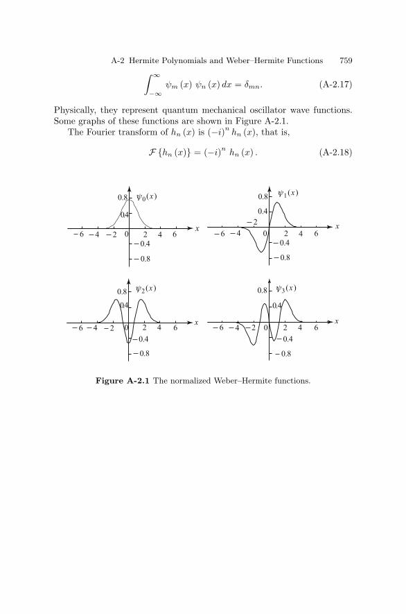
A-2 Hermite Polynomials and Weber–Hermite Functions 759∫ ∞
−∞ψm (x) ψn (x) dx = δmn. (A-2.17)
Physically, they represent quantum mechanical oscillator wave functions.Some graphs of these functions are shown in Figure A-2.1.
The Fourier transform of hn (x) is (−i)nhn (x), that is,
F hn (x) = (−i)nhn (x) . (A-2.18)
Figure A-2.1 The normalized Weber–Hermite functions.

Bibliography
The following bibliography is not, by any means, a complete one for thesubject. For the most part, it consists of books and papers to which referenceis made in text. Many other selected books and papers related to materialin this book have been included so that they may serve to stimulate newinterest in future advanced study and research.
[1] Ablowitz, M.J. and Segur, H., Solitons and Inverse Scattering Trans-form, SIAM, Philadelphia (1981).
[2] Arnold, V.I., Ordinary Differential Equations, Springer-Verlag, NewYork (1992).
[3] Bateman, H., Partial Differential Equations of MathematicalPhysics, Cambridge University Press, Cambridge (1959).
[4] Becker, A.A., The Boundary Element Method in Engineering, Mc-Graw Hill, New York (1992).
[5] Benjamin, T.B., Bona, J.L., and Mahony, J.J., Model equations forlong waves in nonlinear dispersive systems, Phil. Trans. Roy. Soc.A272 (1972) 47–78.
[6] Berg, P. and McGregor, J., Elementary Partial Differential Equa-tions, Holden-Day, New York (1966).
[7] Birkhoff, G. and Rota, G-C., Ordinary Differential Equations(Fourth Edition), John Wiley and Sons, New York (1989).
[8] Boas, M.L., Mathematical Methods in the Physical Sciences, JohnWiley, New York (1966).
[9] Broman, A., Introduction to Partial Differential Equations: fromFourier Series to Boundary-Value Problems, Addison-Wesley, Read-ing, Massachusetts (1970).
[10] Brown, J.W. and Churchill, R.V., Fourier Series and BoundaryValue Problems (Fifth Edition), McGraw-Hill, New York (1993).
[11] Burgers, J.M., A mathematical model illustrating the theory of tur-bulence, Adv. Appl. Mech. 1 (1948) 171–191.
[12] Byerly, W.E., Fourier Series, Dover Publications, New York (1959).[13] Carleson, L., On the convergence and growth of partial sums of
Fourier Series, Acta Mathematica, 116 (1966) 135–157.[14] Carslaw, H.S., Introduction to the Theory of Fourier Series and In-
tegrals, Dover Publications, New York (1950).

762 Bibliography
[15] Carslaw, H.S. and Jaeger, J.C., Operational Methods in AppliedMathematics, Oxford University Press, London (1949).
[16] Carslaw, H.S. and Jaeger, J.C., Conduction of Heat in Solids (SecondEdition), Oxford University Press, Oxford (1986).
[17] Cartan, E., Lecons sur les invariants int egraux, Hermann, Paris(1922).
[18] Churchill, R.V., Operational Mathematics (Third Edition), McGraw-Hill, New York (1972).
[19] Clough, R.W., The finite element method after twenty five years; Apersonal view, Computer Structures 12 (1980) 361–370.
[20] Coddington, E.A. and Levinson, N., Theory of Ordinary DifferentialEquations, McGraw-Hill, New York (1955).
[21] Cole, R., Theory of Ordinary Differential Equation, Appleton-Century-Crofts (1968).
[22] Copson, E.T., Asymptotic Expansions, Cambridge University Press,Cambridge (1965).
[23] Coulson, C.A. and Jeffrey, A., Waves: A Mathematical Approach toCommon Types of Wave Motion (Second Edition), Longman, Lon-don (1977).
[24] Courant, R., Variational methods for the solutions of problems ofequilibrium and vibrations, Bull. Amer. Math. Soc. 49 (1943) 10–30.
[25] Courant, R. and Hilbert, D., Methods of Mathematical Physics, Vol-ume 1 (1953), Volume 2 (1962), Interscience, New York.
[26] Courant, R., Friedrichs, K., and Lewy, H., Uber die partiellen dif-ferenzengleichungen de mathematischen Physik, Mathematische An-nalen 100 (1928) 32–74.
[27] Crank, J., Mathematics of Diffusion (Second Edition), ClarendonPress, Oxford (1975).
[28] Crank, J. and Nicholson, P., A practical method for numerical eval-uation of solutions of partial differential equations of the heat con-duction type, Proc. Camb. Phil. Soc. 43 (1947) 50–67.
[29] Davis, H.F., Fourier Series and Orthogonal Functions, Allyn andBacon, New York (1963).
[30] Debnath, L., On asymptotic treatment of the transient developmentof surface waves, Appl. Sci. Res. 21 (1969) 24–36.
[31] Debnath, L., Unsteady axisymmetric capillary-gravity waves in aviscous liquid, Indian J. Pure and Appl. Math. 14 (1983) 540–553.
[32] Debnath, L., Nonlinear Waves, Cambridge University Press, Cam-bridge, England (1983).
[33] Debnath, L., Solitons and the inverse scattering transforms, Bull.Cal. Math. Soc. 84 (1992) 475–504.
[34] Debnath, L., Nonlinear Water Waves, Academic Press, Boston(1994).

Bibliography 763
[35] Debnath, L., Integral Transforms and Their Applications, CRCPress, Boca Raton, Florida (1995).
[36] Debnath, L., Some nonlinear evolution equations in water waves, J.Math. Anal. Appl. 251 (2000) 488–503.
[37] Debnath, L., Nonlinear dynamics of water waves and breaking phe-nomena, Proc. Indian Nat. Sci. Acad. Special Volume (2002) 683–753.
[38] Debnath, L., Fractional integral and fractional partial differentialequation in fluid mechanics, Fractional Calculus Appl. Analysis 6(2003) 119–155.
[39] Debnath, L., Recent applications of fractional calculus to science andengineering, Internat. J. Math. & Math. Sci. 2003, No. 54 (2003)3413–3442.
[40] Debnath, L., Nonlinear Partial Differential Equations for Scientistsand Engineers (Second Edition), Birkhauser Verlag, Boston (2005).
[41] Debnath, L. and Bhatta, D., On solutions to few linear fractional in-homogeneous partial differential equations in fluid mechanics, Frac-tional Calculus Appl. Analysis 7 (2004) 21–36.
[42] Debnath, L. and Bhatta, D., Integral Transforms and Their Appli-cations (Second Edition), CRC Press, Boca Raton, Florida (2006).
[43] Debnath, L. and Mikusinski, P., Introduction to Hilbert Spaceswith Applications (Third Edition), Elsevier Academic Press, London(2005).
[44] Debnath, L. and Rollins, D., The Cauchy–Poisson waves in an invis-cid rotating stratified liquid, Internat. J. Nonlinear Mech. 27 (1992)405–412.
[45] Debnath, L. and Shivamoggi, B.K., Three-dimensional nonlinearSchrodinger equation for finite-amplitude gravity waves in a fluid,Nuovo Cimento 94B (1986) 140–148; 99B (1987) 247.
[46] Debnath, L. and Shivamoggi, B.K., Pseudo-variational principles andnonlinear surface waves in a dissipative fluid, Internat. J. NonlinearMech. 25 (1990) 61–65.
[47] Dennemeyer, R., Partial Differential Equations and Boundary ValueProblems, McGraw-Hill, New York (1968).
[48] Ditkin, V.A. and Prudnikov, A.P., Integral transforms and Opera-tional Calculus, Pergamon Press, Oxford (1965).
[49] Doetsch, G., Introduction to the Theory and Applications of theLaplace Transformation (Translated by Walter Nader), SpringerVerlag, New York (1970).
[50] Duff, G.F.D., Partial Differential Equations, University of Toronto,Toronto (1956).
[51] Duff, G.F.D. and Naylor, D., Differential Equations of Applied Math-ematics, John Wiley, New York (1966).

764 Bibliography
[52] Dutta, M. and Debnath, L., Elements of the Theory of Ellipticand Associated Functions with Applications, World Press, Calcutta(1965).
[53] Epstein, B., Partial Differential Equations, McGraw-Hill, New York(1962).
[54] Erdelyi, A., Magnus, W., Oberhettinger, F. and Tricomi, F., Tables ofIntegral Transforms (Vols. I and II), McGraw-Hill, New York (1954).
[55] Folland, G.B., Fourier Analysis and Its Applications, Brooks/ColePublishing Company, Pacific Grove, California (1992).
[56] Forsythe, G.E. and Wasow, W.R., Finite-Difference Methods for Par-tial Differential Equations, John Wiley, New York (1967).
[57] Fourier, J.B.J., The Analytical Theory of Heat (Translated by A.Freeman), Dover Publications, New York (1955).
[58] Fox, C., An Introduction to the Calculus of Variations, Oxford Uni-versity Press, Oxford (1963).
[59] Garabedian, P.R., Partial Differential Equations, John Wiley, NewYork (1964).
[60] Gelfand, I.M. and Fomin, S.V., Calculus of Variations (Translatedby R.A. Silverman), Prentice-Hall, Englewood Cliffs, New Jersey(1963).
[61] Ghosh, K.K. and Debnath, L., Some exact solutions of nonlinearshallow water equations, Internal. J. Nonlinear Mech. 31 (1997) 104–108.
[62] Greenberg, M., Applications of Green’s Functions in Science andEngineering, Prentice-Hall, Englewood Cliffs, New Jersey (1971).
[63] Grunberg, G., A new method of solution of certain boundary prob-lems for equations of mathematical physics permitting of a separationof variables, J. Phys. 10 (1946) 301–320.
[64] Haberman, R., Mathematical Models: Mechanical Vibrations, Popu-lation Dynamics and Traffic Flow, Prentice Hall, Englewood Cliffs,New Jersey (1977).
[65] Hadamard, J., Lectures on Cauchy’s Problem in Linear Partial Dif-ferential Equations, Dover Publications, New York (1952).
[66] Haight, F.A., Mathematical Theories of Traffic Flow, AcademicPress, New York (1963).
[67] Hellwig, G., Partial Differential Equations, Blaisdell, Waltham, Mas-sachusetts (1964).
[68] Hildebrand, F., Methods of Applied Mathematics, Prentice-Hall, En-glewood Cliffs, New Jersey (1965).
[69] Huebuer, K.H., Dewhirst, D.L., Smith, D.L., and Byrom, T.G., TheFinite Element Method for Engineers (Fourth Edition), John Wiley& Sons, New York (2001).
[70] Irving, J. and Mullineux, N., Mathematics in Physics and Engineer-ing, Academic, New York (1959).

Bibliography 765
[71] Jackson, D., Fourier Series and Orthogonal Polynomials, Mathemat-ical Association of America Monograph (1941).
[72] Jaswon, M.A., Integral equation method in potential theory. I, Proc.R. Soc. London, A 275 (1963) 23–32.
[73] Jeffrey, A., Advanced Engineering Mathematics, Academic Press,Boston (2002).
[74] Jeffrey, A. and Engelbrecht, J., Nonlinear Waves in Solids, Springer-Verlag, New York (1994).
[75] Jeffrey, A. and Kawahara, T., Asymptotic Methods in Nonlin-ear Wave Theory, Pitman Advanced Publishing Program, Boston(1982).
[76] Jeffrey, A. and Taniuti, T., Nonlinear Wave Propagation, AcademicPress, New York (1964).
[77] Jeffreys, H., Operational Methods in Mathematical Physics, Cam-bridge University Press, New York (1931).
[78] Jeffreys, J. and Jeffreys, B.S., Methods of Mathematical Physics(Third Edition), Cambridge University Press, Cambridge (1956).
[79] John, F., Partial Differential Equations (Fourth Edition), Springer-Verlag, New York (1982).
[80] Johnson, R.S., The KdV equation and related problems in waterwave theory, in Nonlinear Waves (ed. L. Debnath), 25–43, Cam-bridge University Press, Cambridge (1983).
[81] Johnson, R.S., A Modern Introduction to the Mathematical Theoryof Water Waves, Cambridge University Press, Cambridge (1997).
[82] Jones, D.S., Generalized Functions, Academic Press, New York(1966).
[83] Kantorovich, L. and Krylov, V., Approximate Methods in HigherAnalysis, Interscience, New York (1958).
[84] Keener, J.P., Principles of Applied Mathematics: Transforma-tion and Approximation, Addition-Wesley, Reading, Massachusetts(1988).
[85] Keller, H., Numerical Methods for Two Point Boundary Value Prob-lems, Blaisdell, Waltham, Massachusetts (1968).
[86] Knobel, R., An Introduction to the Mathematical Theory of Waves,American Mathematical Society, Providence (1999).
[87] Korteweg, D.J. and de Vries, G., On the change of form of longwaves advancing in a rectangular canal, and on a new type of longstationary waves, Phil. Mag. 39 (1895) 422–443.
[88] Koshlayokov, N.S., Smirnov, M.M. and Gliner, E.B., DifferentialEquations of Mathematical Physics, Holden-Day, New York (1964).
[89] Kreider, D., Kuller, R., Ostberg, D., and Perkins, F., An Introductionto Linear Analysis, Addition-Wesley, Reading, Massachusetts (1966).
[90] Kreyszig, E., Advanced Engineering Mathematics (Seventh Edition),John Wiley, New York (1993).

766 Bibliography
[91] Lamb, H., Hydrodynamics (Sixth Edition), Cambridge UniversityPress, Cambridge, England (1932).
[92] Lax, P.D., Weak solutions of nonlinear hyperbolic equations and theirnumerical computation, Comm. Pure Appl. Math. 7 (1954) 159–193.
[93] Lax, P.D., The initial-value problem for nonlinear hyperbolic equa-tions in two independent variables, Ann. Math. Stud. (Princeton) 33(1954) 211–299.
[94] Lax, P.D., Hyperbolic systems of conservation law, II, Comm. PureAppl. Math. 10 (1957) 537–566.
[95] Lax, P.D., Partial Differential Equations, Lectures on HyperbolicEquations, Stanford University Press (1963).
[96] Lax, P.D., Development of singularities of solutions of nonlinear hy-perbolic partial differential equations, J. Math. Phys. 5 (1964) 611–613.
[97] Lax, P.D., Integrals of nonlinear equations of evolution and solitarywaves, Comm. Pure Appl. Math. 21 (1968) 467–490.
[98] Lax, P.D., The formation and decay of shock waves, Amer. Math.Monthly 79 (1972) 227–241.
[99] Lax, P.D., Hyperbolic Systems of Conservation Lays and the Math-ematical Theory of Shock Waves, Society for Industrial and AppliedMathematics, Philadelphia (1973).
[100] Lax, P.D., Periodic solutions of the Korteweg–de Vries equation,Comm. Pure Appl. Math. 28 (1975) 141–188.
[101] Lax, P.D., A Hamiltonian approach to the KdV and other equa-tions, in Nonlinear Evolution Equations (ed. M. Crandall), AcademicPress, New York (1978) 207–224.
[102] Lax, P.D. and Wendroff, B., Systems of Conservation Laws, Comm.Pure Appl. Math. 13 (1960) 217–237.
[103] Leibovich, S. and Seebass, A.R., Nonlinear Waves, Cornell Univer-sity Press, Ithaca and London (1972).
[104] Lighthill, M.J., Introduction to Fourier Analysis and GeneralizedFunctions, Cambridge University Press, Cambridge (1964).
[105] Lighthill, M.J., Waves in Fluids, Cambridge University Press, Cam-bridge (1980).
[106] Logan, J.D., Applied Mathematics (Second Edition), John Wiley,New York (1997).
[107] Mainardi, F., On the initial-value problem for the fractionaldiffusion-wave equation, in Waves and Stability in Continuous Media(ed. S. Rionero and T. Ruggeri), World Scientific, Singapore (1994)246–251.
[108] Mainardi, F., The time fractional diffusion-wave equation, Ra-diofisika 38 (1995) 20–36.
[109] Mainardi, F., Fractional relaxation-oscillation and fractionaldiffusion-wave phenomena, Chaos, Solitons, Fractals 7 (1996) 1461–1477.

Bibliography 767
[110] McLachlan, N.W., Complex Variable and Operational Calculus withTechnical Applications, Cambridge University Press, London (1942).
[111] McLachlan, N.W., Modern Operational Calculus, Macmillan, London(1948).
[112] Mikhlin, S.G., Variational Methods in Mathematical Physics, Perg-amon Press, Oxford (1964).
[113] Mikhlin, S.G., Linear Equations of Mathematical Physics, Holt,Rinehart and Winston, New York (1967).
[114] Miller, K.S., Partial Differential Equations in Engineering Problems,Prentice Hall, Englewood Cliffs, New Jersey (1953).
[115] Mitchell, A.R. and Griffiths, D.F., The Finite Difference Method inPartial Differential Equations, John Wiley, New York (1980).
[116] Morse, P.M. and Freshbach, H., Methods of Theoretical Physics, Vol-ume 1 and 2, McGraw-Hill, New York (1953).
[117] Myint-U, T., Ordinary Differential Equations, Elsevier North Hol-land, Inc., New York (1978).
[118] Nigmatullin, R.R., The realization of the generalized transfer equa-tion in a medium with fractal geometry, Phys. Sta. Sol. (b) 133(1986) 425–430.
[119] Petrovsky, I., Lectures on Partial Differential Equations, Inter-science, New York (1954).
[120] Picard, E., Trait e d’Analyse, Gauthier-Villars, Paris (1896).[121] Pinkus, A. and Zafrany, S., Fourier Series and Integral Transforms,
Cambridge University Press, Cambridge (1997).[122] Pipes, L.A., Applied Mathematics for Engineers and Physicists,
McGraw-Hill, New York (1958).[123] Qiao, Z., Generation of the hierarchies of solitons and general-
ized structure of the commutator representation, Acta. Appl. Math.Sinica 18 (1995) 287–301.
[124] Qiao, Z. and Strampp, W., Negative order MKdV hierarchy and anew integrable Neumann-like system, Physica A 313 (2002) 365–380.
[125] Raven, R.H., Mathematics of Engineering Systems, McGraw-Hill,New York (1966).
[126] Rayleigh, Lord, The Theory of Sound, Vol. I (1894), Vol. 2 (1896),Dover Publications, New York.
[127] Reif, F., Fundamentals of Statistical and Thermal Physics, McGrawHill, New York (1965).
[128] Richtmyer, R.D. and Morton, K.W., Difference Methods for initial-value problems, Interscience, New York (1967).
[129] Roach, G.F., Green’s Functions (Second Edition), Cambridge Uni-versity Press, Cambridge (1982).
[130] Rogosinski, W.W., Fourier Series, Chelsea, London (1950).[131] Sagan, H., Boundary and Eigenvalue Problems in Mathematical
Physics, John Wiley, New York (1966).[132] Sansone, G., Orthogonal Functions, Interscience, New York (1959).

768 Bibliography
[133] Schneider, W.R. and Wyss, W., Fractional diffusion and wave equa-tions, J. Math. Phys. 30 (1989) 134–144.
[134] Schwartz, L., Theorie des distributions, Volume I (1950) and VolumeII (1951), Herman and Cie, Paris.
[135] Scott, E.J., Transform Calculus with an Introduction to ComplexVariables, Harper, New York (1955).
[136] Seeley, R., An Introduction to Fourier Series and Integrals, W.A.Benjamin, New York (1966).
[137] Smirnov, V.I., Integral Equations and Partial Differential Equations,Addison-Wesley, Reading, Massachusetts (1964).
[138] Smith, G.D., Numerical Solution of the Partial Differential Equa-tions (Third Edition), Clarendon Press, Oxford (1985).
[139] Smith, M.G., Introduction to the Theory of Partial Differential Equa-tions, Van Nostrand, Princeton, New Jersey (1967).
[140] Smoller, J., Shock Waves and Reaction-Diffusion Equations (SecondEdition), Springer-Verlag, New York (1995).
[141] Sneddon, I.N., Fourier Transforms, McGraw-Hill, New York (1951).[142] Sneddon, I.N., Elements of Partial Differential Equations, McGraw-
Hill, New York (1957).[143] Sneddon, I.N., The Use of Integral Transforms, McGraw-Hill, New
York (1972).[144] Sobolev, S.L., Partial Differential Equations of Mathematical
Physics, Addison-Wesley, Reading, Massachusetts (1964).[145] Soewono, E. and Debnath, L., Asymptotic stability of solutions of
the generalized Burgers equation, J. Math. Anal. Appl. 153 (1990)179–189.
[146] Soewono, E. and Debnath, L., Classification of self-similar solutionsto a generalized Burgers equation, J. Math. Anal. Appl. 184 (1994)389–398.
[147] Sokolnikoff, I.S., Mathematical Theory of Elasticity, McGraw-Hill,New York (1956).
[148] Sokolnikoff, I.S. and Redheffer, R.M., Mathematics of Physics andModern Engineering, McGraw-Hill, New York (1966).
[149] Sommerfeld, A., Partial Differential Equations in Physics, AcademicPress, New York (1964).
[150] Stakgold, I., Green’s Functions and Boundary Value Problems,Wiley-Interscience, New York (1979).
[151] Stoker, J.J., Water Waves, Interscience, New York (1957).[152] Stoker, G., On the theory of oscillatory waves, Trans. Camb. Phil.
Soc. 8 (1847) 197–229.[153] Strauss, W.A., Partial Differential Equations: An Introduction, John
Wiley, New York (1992).[154] Symm, G.T., Integral equation method in potential theory, Proc.
Roy Soc. London A275 (1963) 33–46.

Bibliography 769
[155] Tikhonov, A.N. and Samarskii, A.A., Equations of MathematicalPhysics, Macmillan, New York (1963).
[156] Titchmarsh, E.C., Eigenfunction Expansions Associated with Second-Order Differential Equations, Oxford University Press, Oxford(1946).
[157] Titchmarsh, E.C., An Introduction to the Theory of Fourier Inte-grals, Oxford University Press, Oxford (1962).
[158] Toda, M., Vibration of a chain with nonlinear interaction, J. Phys.Soc. Japan 22 (1967) 431–436.
[159] Tolstov, G.P., Fourier Series, Prentice-Hall, Englewood Cliffs, NewJersey (1962).
[160] Tranter, C.J., Integral Transforms in Mathematical Physics (ThirdEdition), John Wiley, New York (1966).
[161] Tychonov, A.N. and Samarskii, A.A., Partial Differential Equationsof Mathematical Physics, Holden-Day, New York (1964).
[162] Watson, G.N., A Treatise on the Theory of Bessel Functions, Cam-bridge University Press, Cambridge (1966).
[163] Webster, A.G., Partial Differential Equations of MathematicalPhysics, Dover Publications, New York (1955).
[164] Weinberger, H., A First Course in Partial Differential Equations,Blaisdell, Waltham, Massachusetts (1965).
[165] Whitham, G.B., A general approach to linear and nonlinear disper-sive waves using a Lagrangian, J. Fluid Mech. 22 (1965) 273–283.
[166] Whitham, G.B., A new approach to problems of shock dynamics.Part I. Two dimensional problems, J. Fluid Mech. 2 (1975) 146–171.
[167] Whitham, G.B., Linear and Nonlinear Waves, John Wiley, New York(1976).
[168] Whittaker, E.T. and Watson, G.N., A Course on Modern Analysis,Cambridge University Press, Cambridge (1952).
[169] Widder, D.V., The Laplace Transform, Princeton University Press,Princeton, New Jersey (1941).
[170] Zabusky, N.J. and Kruskal, M.D., Interaction of Solitons in a Col-lisionless Plasma and Recurrence of Initial States, Phys. Rev. Lett.15 (1965) 240–243.
[171] Zakharov, V.E. and Shabat, A.B., Exact Theory of Two-DimensionalSelf-Focusing and One-Dimensional Self Modulation of Waves inNonlinear Media, Sov. Phys. JETP 34 (1972) 62–69.
[172] Zakharov, V.E. and Shabat, A.B., Interaction Between Solitons in aStable Medium, Sov. Phys. JETP 37 (1974) 823–828.
[173] Zauderer, E., Partial Differential Equations of Applied Mathematics(Second Edition), John Wiley, New York (1989).
[174] Zienkiewicz, O.C. and Cheung, Y.K., Finite elements in the solutionsof field problems, Engineer. 220 (1965) 370–507.
[175] Zienkiewicz, O.C. and Taylor, R.L., The Finite Element Method,McGraw-Hill, New York (1989).

770 Bibliography
Tables and Formulas
[176] Campbell, G.A. and Foster, R.M., Fourier Integrals for PracticalApplications, Van Nostrand, New York (1948).
[177] Erdelyi, A., Magnus, W., Oberhettinger, F. and Tricomi, F. G.,Higher Transcendental Functions, Volumes I, II, and III, McGraw-Hill, New York (1953).
[178] Jeffrey, A., Handbook of Mathematical Formulas and Integrals (ThirdEdition), Elsevier Academic Press, New York (2004).
[179] Jhnke, E., Emde, F., and Losch, F., Tables of Higher Functions,McGraw-Hill, New York (1960).
[180] Magnus, W., Oberhettinger, F., and Soni, R.P., Formulas and Theo-rems for the Special Functions of Mathematical Physics (Third Edi-tion), Springer-Verlag, Berlin (1966).
[181] Oberhettinger, F., Tables of Bessel Transforms, Springer-Verlag,New York (1972).
[182] Marichev, O.I., Handbook of Integral Transforms of Higher Transcen-dental Functions: Theory and Algorithmic Tables, Ellis Horwood,Chichester, (1982).
[183] Zeidler, E., Oxford User’s Guide to Mathematics, Oxford UniversityPress, Oxford (2004).
Problem Books
[184] Budak, B.M., Samarskii, A.A., and Tikhonov, A.N., A Collection ofProblems on Mathematical Physics, Macmillan, New York (1964).
[185] Lebedev, N.N., Skalskaya, I.P., and Uflyand, Y.S., Problems ofMathematical Physics, Prentice-Hall, Englewood Cliffs, New Jersey(1965).
[186] Smirnov, M.M., Problems on the Equations of Mathematical Physics,Noordhoff (1967).

Index
Abel’s problem, 529acceleration parameter, 620adjoint, 630adjoint operator, 143, 296angular frequencies, 239associated Legendre function, 307,
384, 385
backward first difference, 602Banach space, 629Bender–Schmidt explicit formula, 613Benjamin and Feir instability, 586, 587Benjamin, Bona and Mahony (BBM)
equation, 580Bernoulli, 3Bessel equation, 289, 375Bessel function, 289Bessel function of the first kind, 290Bessel function of the second kind, 291Bessel’s inequality, 175, 286biharmonic equation, 64, 404biharmonic wave equation, 64binding energy, 389Birkhoff, 10Blasius problem, 527Bohr radius, 388Born, 10bound state, 392boundary conditions, 15boundary element method, 668boundary integral equation method,
668boundary-value problem, 308, 329bounded, 630
Boussinesq equation, 543, 675Brachistochrone problem, 678Burgers equation, 81, 563, 569
canonical form, 49, 50, 95, 96Cauchy, 4–6Cauchy data, 119Cauchy problem, 3, 15, 36, 118Cauchy sequence, 629Cauchy–Kowalewskaya theorem, 6,
120Cauchy–Poisson problem, 530Cauchy–Poisson wave problem, 485Cauchy–Riemann equations, 5central first difference, 602CFL condition, 609characteristic, 34characteristic base curve, 34characteristic curve, 2, 33, 35, 94, 537,
555characteristic direction, 33characteristic equation, 33, 94, 120characteristic initial-value problem,
150characteristic velocities, 549Clairaut, 2cnoidal wave, 578commutator, 591compatibility condition, 349complete integral, 29complete solution, 29complex Fourier series, 194conservation law, 80conservation of vorticity, 89

772 Index
consistent, 604continuity equation, 85continuity theorem, 333convergence, 602convolution, 448, 467convolution property, 497convolution theorem, 448, 467Courant, 663Courant parameter, 608Courant–Friedrichs–Lewy convergence
criterion, 608Crank–Nicolson formula, 626Crank–Nicolson implicit formula, 625cummulative truncation, 603cylindrical wave equation, 155, 156
d’Alembert, 3d’Alembert solution, 3, 123d’Alembertian, 65damped wave equation, 84de Broglie wave, 542Debnath, 482, 485, 515, 517, 519, 521,
588, 590density, 580differential operators, 16differentiation, 445, 464differentiation theorem, 209diffusion equation, 514, 566, 569diffusion equation in a finite medium,
482diffusion in a finite medium, 483diffusive, 97dilatational, 73Dirac delta function, 446, 470Dirichlet, 5Dirichlet boundary-value problem, 5Dirichlet condition, 235Dirichlet kernel, 203Dirichlet problem, 330, 416Dirichlet problem for a circle, 334Dirichlet problem for a cylinder, 363Dirichlet problem for a rectangle, 343,
348Dirichlet problem for a sphere, 367Dirichlet problem for circular annulus,
340discontinuities, 44discrete energy spectrum, 387discrete values of energy, 392
discretization error, 603dispersion relation, 541, 573dispersion relation for water waves,
542dispersive, 97, 542dispersive wave, 540domain of dependence, 123, 125double Fourier series, 212, 213Du Fort–Frankel explicit algorithm,
614Duhamel formula, 481, 533Duhamel principle, 165
eigenfunction, 237, 274eigenvalue, 237eigenvalue problem, 236Einstein, 10elliptic, 92elliptic equation, 111energy, 241energy density, 547energy equation, 163energy flux, 547energy integral, 163envelope, 48equation
Benjamin, Bona and Mahony(BBM), 580
Bessel, 289, 375biharmonic, 64, 404biharmonic wave, 64Boussinesq, 543, 675Burgers, 81, 563, 569Cauchy–Riemann, 5characteristic, 33, 94, 120continuity, 85cylindrical wave, 155, 156damped wave, 84diffusion, 514, 566, 569elliptic, 111energy, 163Euler, 38, 65, 88, 89, 100Euler–Lagrange, 9, 629, 633, 634,
646Euler–Poisson–Darboux, 598Fokker–Planck, 62, 90, 264, 436fractional axisymmetric wave-
diffusion, 518fractional diffusion, 510, 514

Index 773
fractional diffusion-wave, 511fractional partial differential
equation, 510fractional Schrodinger, 520fractional wave, 512Hamilton–Jacobi, 9heat, 64, 76, 84Helmholtz, 64, 75, 85, 330, 372, 494Hermite, 323hyperbolic, 111Klein–Gordon (KG), 64, 542Korteweg–de Vries (KdV), 88, 542,
574, 593Lagrange, 8Laguerre, 323Laplace, 3, 64, 330, 361Lax, 592Legendre, 302, 384Legendre associated, 306linear Schrodinger, 82, 582linearized Korteweg–de Vries
(KdV), 83Maxwell, 3, 84Navier, 72, 73nonhomogeneous wave, 139nonlinear, 29nonlinear diffusion, 80nonlinear hyperbolic, 550nonlinear Schrodinger (NLS), 83,
583, 585parabolic , 111partial differential, 12Poisson, 64, 85, 330, 429potential, 3, 5quasi-linear partial differential, 28,
89Schrodinger, 64, 317, 330, 382, 404,
542, 581spherical wave, 153Sturm–Liouville, 274Tchebycheff, 323telegraph, 64, 84, 87, 147, 436time dependent Schrodinger, 382vorticity, 89wave, 64, 67, 69, 73, 511, 535, 536,
542wave and heat, 372Whitham, 545, 548
equation for vibration of a beam, 542
error function, 452Euler, 3Euler equation, 38, 65, 88, 89, 100Euler’s equation of motion, 85Euler–Lagrange equation, 9, 629, 633,
634, 646Euler–Lagrange variational principle,
634Euler–Lagrange variational problem,
632Euler–Poisson–Darboux equation, 598even extension, 192explicit finite difference methods, 608
Fermat, 7Fermat principle in optics, 635Fermi–Pasta–Ulam model, 88fine structure corrections, 389finite difference approximations, 602finite element method, 663finite Fourier cosine transform, 500finite Fourier sine transform, 499finite Hankel transform, 505first canonical form, 95Fitzgerald, 10five-point formula, 621flood wave, 552flux, 580Fokker–Planck equation, 62, 90, 264,
436Forsyth, 6forward first difference, 602Fourier, 4Fourier coefficients, 173Fourier cosine transform, 443, 456, 500Fourier integral representation, 218,
219Fourier integral theorem, 4, 217Fourier integrals, 214Fourier method, 232Fourier series, 171, 173Fourier sine integral formula, 443Fourier sine transform, 443, 457Fourier transform, 440Fourier–Legendre series, 284fractional axisymmetric wave-diffusion
equation, 518fractional derivative, 480, 482, 499fractional diffusion equation, 510, 514

774 Index
fractional diffusion-wave equation, 511fractional partial differential equation,
510fractional Rayleigh problem, 517fractional Schrodinger equation, 520fractional Stokes and Rayleigh
problem, 515fractional unsteady Couette flow, 517fractional wave equation, 512fundamental harmonic, 239fundamental period, 169fundamental solution, 451
Galerkin approximation method, 655Gauss, 5Gaussian probability density, 404general Parseval relation, 227general solution, 30, 107generalized coordinates, 638generalized solution, 130Gibbs, 186Gibbs phenomenon, 181, 185, 208, 225global convergence, 174Goursat, 6Goursat problem, 149gravitational potential, 76Green, 5Green’s function, 312, 407–409, 451group velocities, 541group velocity, 546
Hadamard, 3Hadamard example, 121Hamilton, 8Hamilton equations of motion, 8, 643Hamilton’s principle, 8, 636Hamilton–Jacobi equation, 9Hamiltonian, 382Hamiltonian function H, 642Hankel transform, 489harmonic, 330harmonic function, 5, 330harmonic oscillator, 320heat conduction in a rectangular
volume, 381heat equation, 64, 76, 84heat flow in a rectangular plate, 375Heaviside unit step function, 453, 470
Helmholtz equation, 64, 75, 85, 330,372, 494
Helmholtz operator, 415, 418Hermite equation, 323Hermite function, 265Hermite polynomials, 320Hilbert, 10Hilbert space, 629homogeneous, 13, 29hydrogen atom, 382hyperbolic, 92hyperbolic equation, 111
ill-posed problem, 549implicit finite difference method, 624implicit Richardson formula, 626impulse function, 454infinite square well potential, 389initial boundary-value problem, 15initial condition, 15, 37initial data, 37initial-value problem, 3, 15, 36, 118inner product, 629integral surface, 33integration, 465integration theorem, 209inverse Fourier cosine transform, 500inverse Fourier sine transform, 500inverse Fourier transform, 440inverse Hankel transform, 489, 505inverse Laplace transform, 461inverse Mellin transformation, 496irrotational, 73
Jacobi, 6, 9Jacobian, 411
Kantorovich method, 659Klein, 10Klein–Gordon (KG) equation, 64, 542Korteweg–de Vries (KdV) equation,
88, 542, 574, 593Kowalewskaya, 6
Lagrange, 2, 3Lagrange equation, 8Lagrange equations of motion, 639Lagrange identity, 279, 297Lagrangian, 8Laguerre equation, 323

Index 775
Laplace, 4Laplace equation, 3, 64, 330, 361Laplace operator, 65, 72, 372Laplace transform, 461law of the conservation of energy, 643Lax equation, 592Lax equivalence theorem, 604Lax pair, 591Lax–Wendroff explicit method, 605Lax–Wendroff second-order finite
difference scheme, 606leap frog algorithm, 607, 610Legendre, 5Legendre associated equation, 306Legendre equation, 302, 384Legendre function, 302, 370Legendre function of the first kind,
304Legendre function of the second kind,
305Legendre polynomial, 304Lerch, 465Lie, 6Liebmann iterative method, 619, 620Lighthill, 446linear, 13, 28, 630linear integral superposition principle,
19linear Schrodinger equation, 82, 582linear superposition principle, 19linearity, 444, 463linearized Korteweg–de Vries (KdV)
equation, 83Liouville, 6, 7Liouville theorem, 352local convergence, 174local frequency, 546local truncation error, 604local wavenumber, 546longitudinal wave velocity, 73Lorentz, 10lowest state energy, 319
Mach number, 86magnetic quantum number, 385Mainardi, 514Maupertius, 7maximum principle, 332Maxwell, 3
Maxwell equation, 3, 84mean value theorem, 338, 618mean-square convergence, 173, 174Mellin transform, 496method of characteristics, 35method of images, 420method of majorants, 6method of separation of variables, 3,
51, 232Michelson, 186minimum principle, 332Mittag-Leffler function, 510mixed condition, 235Monge, 2, 5Monge axis, 33Monge cone, 35
Navier, 6Navier equations, 72, 73Neumann, 5Neumann boundary-value problem, 5Neumann condition, 235Neumann problem, 331, 341, 430Newton, 2Newton second law of motion, 637nodes, 239Noether, 10nonhomogeneous, 13, 29nonhomogeneous wave equation, 139nonlinear, 13nonlinear diffusion equation, 80nonlinear dispersion relation, 585nonlinear equation, 29nonlinear hyperbolic equation, 550nonlinear initial-value problem, 539nonlinear Schrodinger (NLS) equation,
83, 583, 585norm, 170, 450, 629normal modes, 239normal stresses, 69numerical characteristics, 609
odd extension, 192orbital quantum member, 385order, 13orthogonal, 170, 277orthonormal system, 170Ostrogradsky, 5, 8overtones, 239

776 Index
parabolic, 92parabolic equation, 111Parseval formula, 195, 449, 497Parseval relation, 176, 212, 491Parseval’s equality, 286partial differential equation, 12particular solution, 30period, 169periodic, 169periodic extension, 190, 192phase, 541phase function, 459Picard, 11piecewise continuous, 168piecewise smooth, 168piston problem, 558, 559Planck constant, 318, 382Plateau, 7Poincare, 8Poincare–Cartan invariant, 9point phase, 459pointwise approximations, 663pointwise convergence, 173pointwise convergence theorem, 202Poisson, 4Poisson equation, 64, 85, 330, 429Poisson integral formula, 337, 428, 451Poncelet, 5positive definite, 631potential, 5potential energy, 382potential equation, 3, 5power spectrum, 450principal quantum number, 387principle of conservation of energy, 581principle of least action, 7, 636principle of linear superposition, 19principle of superposition, 451progressive wave, 127
quantum number, 319quasi-linear, 13quasi-linear partial differential
equation, 28, 89
radial velocity, 154range of influence, 124Rayleigh, 10Rayleigh layer, 478
Rayleigh problem, 477Rayleigh–Ritz approximation method,
647Rayleigh–Ritz method, 655regular Sturm–Liouville (RLS) system,
274relaxation factor, 620residual, 656residual displacement, 129Richardson explicit finite difference
scheme, 614Richardson iteration formula, 620Riemann function, 148Riemann invariants, 557, 558Riemann method, 142Riemann zeta function, 189, 533Riemann–Lebesgue lemma, 201Robin problem, 331, 422Rodriguez formula, 305rotational waves, 74round-off error, 604Rydberg, 388
sawtooth wave function, 180scalar potential, 74scaling, 445, 463, 492Schrodinger equation, 64, 317, 330,
382, 404, 542, 581second canonical form, 95second shifting, 470self-adjoint, 143, 296, 630semilinear, 28shear stresses, 69shifting, 444, 463shock, 540shock condition, 562shock thickness, 569shock wave, 561signum function, 460similarity variable, 478simple eigenvalue, 277simple harmonic oscillator, 637simple wave, 553simple wave motions, 558singular solution, 30singular Sturm–Liouville (SSL)
system, 297skin friction, 479smooth function, 31

Index 777
Snell law of refraction of light, 636solitary wave, 576, 581, 585soliton, 83, 573, 576solution
complete, 29d’Alembert, 3, 123fundamental, 451general, 30generalized, 130particular, 30singular, 30Stokes steady-state, 478weak, 31
solution surface, 33solutions, 12Sommerfeld radiation condition, 494source point, 429spectral function, 459spherical harmonics, 385spherical symmetric wave, 153spherical wave equation, 153stability, 602stable, 604standing wave, 239stationary phase method, 458stationary point, 459Stokes, 6Stokes expansion, 548Stokes layer, 478Stokes problem, 477Stokes steady-state solution, 478Stokes–Ekman problem, 528Sturm, 7Sturm–Liouville equation, 274Sturm–Liouville operator, 279Sturm–Liouville theory, 6, 273Successive Over-Relaxation (SOR)
scheme, 620superposition principle, 20
linear, 19linear integral, 19
Tchebycheff equation, 323telegraph equation, 64, 84, 87, 147,
436thermal conductivity, 75, 481time dependent Schrodinger equation,
382time invariant function, 581
total kinetic energy, 240total potential energy, 240traffic flow model, 549transform
finite Fourier cosine, 500finite Fourier sine, 499finite Hankel, 505Fourier, 440Fourier cosine, 443, 456, 500Fourier sine, 443, 457Hankel, 489inverse Fourier, 440inverse Fourier cosine, 500inverse Fourier sine, 500inverse Hankel, 489, 505inverse Laplace, 461Laplace, 461Mellin, 496
transverse wave velocity, 72triangular wave, 128triangular wave function, 187, 188truncation error, 602
undular bore, 579uniform and absolute convergence
theorem, 208uniform convergence, 173uniqueness theorem, 333
variational method, 629vector potential, 74vibrating membrane, 67, 372vibrating string problem, 136, 235vibration of a circular membrane, 374von Neumann stability, 610von Neumann’s stability method, 605vorticity equation, 89
wavecnoidal, 578de Broglie, 542dispersive, 540flood, 552progressive, 127rotational, 74shock, 561simple, 553solitary, 576, 581, 585spherical symmetric, 153standing, 239

778 Index
triangular, 128wave and heat equations, 372wave equation, 64, 67, 69, 73, 511, 535,
536, 542waves in three dimensions, 379waves of distortion, 72weak solution, 31Weierstrass, 6Weierstrass approximation theorem,
223
well-posed problem, 16, 124, 166Weyl, 10Weyl fractional integral, 498Whitham, 545, 588Whitham equation, 545, 548Wright function, 511
Zakharov–Shabat (ZS) scheme, 594Zienkiewicz and Cheung, 664