type, number, and dimensional synthesisfaculty.mae.carleton.ca/john_hayes/5507notes/ch3jh.pdf ·...

Chapter 3

Type, Number, and

Dimensional Synthesis

The science of mechanism kinematics is roughly divided in two divergent topics:

analysis and synthesis. Analysis typically involves a defined mechanism and

predicting how either the coupler or the follower will react to specific motions

of the driver. Consider Figure 3.1 for example. It may be that we need to

determine the position of reference point C on the coupler in the relatively

non-moving frame Σ given an input angle ψ and all the link lengths, i.e. the

distances between revolute centers, and position of point C in the coupler frame

E. Alternately, it may be that we wish to determine the pose (position and

orientation) of reference frame E that moves with the coupler in terms of fixed

Figure 3.1: 4R four-bar mechanism.

53

54 CHAPTER 3. TYPE, NUMBER, AND DIMENSIONAL SYNTHESIS

frame Σ for a given input ψ. Another problem we may need to solve is to

determine the change in follower angle ϕ for a change in input angle ψ; or the

kinematic equivalent, determine the motion of follower frame F expressed in Σ

given the input ψ. We will examine analysis in a later chapter.

A fundamentally different problem is that of kinematic synthesis. But, as

we shall see, with some geometric insight, we can use the same approach as for

analysis. By kinematic synthesis we mean the design or creation of a mechanism

to attain specific motion characteristics. In this sense, synthesis is the inverse

of analysis. Synthesis is the very essence of design because it represents the cre-

ation of new hardware to meet particular requirements of motion: displacement;

velocity; acceleration; individually or in combination. Some typical examples of

kinematic synthesis include:

1. Guiding a point along a specific curve, see Figure 3.2a. Examples of such

devices include James Watt’s straight line linkage illustrated in Figure 3.2b

(taken from British Patent 1432, April 28, 1784), automated post-hole

diggers, etc..

(a) Point C is guided along the curve

c to sequential positions C1 to C5.

(b) Watt’s straight line linkage.

Figure 3.2: Guiding a point on a rigid body along a curve.

2. Correlating driver and follower angles in a functional relationship: the

resulting mechanism is a function generator. In essence the mechanism

generates the function ϕ = f(ψ), or vice versa, see Figure 3.3. The func-

tion generator we will examine is a four-bar steering linkage. The function

is known as the Akermann steering condition. Ackermann steering geom-

etry is a geometric arrangement of linkages in the steering of a wheeled

vehicle designed to solve the problem of wheels on the inside and outside

of a turn needing to trace out circles of different radii. The intention of

55

Figure 3.3: Function generator.

Ackermann geometry is to avoid the need for tires to slip sideways when

following the path around a curve. It was invented by the German car-

riage builder Georg Lankensperger in Munich in 1817, then patented by

his agent in England, Rudolph Ackermann (1764-1834) in 1818 for horse-

drawn carriages [1]. The steering function creates the condition that the

Figure 3.4: The steering condition.

normals to the centre of each steerable wheel intersect the line passing

through the centre of the common axle of the non-steerable wheels. The

Akermann steering condition is defined by:

S(∆ψ,∆ϕ) ≡ sin(∆ϕ−∆ψ)− ρ sin(∆ψ) sin(∆ϕ) = 0. (3.1)

In the steering condition ∆ψ and ∆ϕ are the change in input and output

angles, respectively from the input and output dial zeroes, α and β, i.e.


ψ = 0 and ϕ = 0 are not necessarily in the direction of the x-axis, they

may be offset. The quantity ρ is the length ratio b/a, with a the dis-

tance between axles and b the distance between wheel-carrier revolutes,

as illustrated in Figure 3.4.

3. Guiding a rigid body through a finite set of positions and orientations,

as in Figure 3.5a. A good example is a landing gear mechanism which

must retract and extend the wheels, having down and up locked poses

with specific intermediate poses for collision avoidance, see Figure 3.5b.

(a) Motion of coordinate system.(b) Main landing gear.

Figure 3.5: Rigid body guidance (motion generation).

Synthesis for rigid body guidance is also known as the Burmester Problem,

after Ludwig Burmester (1840-1927), Professor of Descriptive Geometry

and Kinematics. His book Lehrbuch der Kinematik [2], is a classic system-

atic and comprehensive treatment of theoretical kinematics as understood

in the late 19th century.

Figure 3.6: Rack-and-pinion drive.

57

Figure 3.7: The line generating linkage where ψ is proportional to R along the

straight line portion of the coupler curve for point R.

4. Trajectory Generation: Position, velocity, and/or acceleration must be

correlated along a curve. Examples include film transport mechanisms

in motion picture projectors. Another example is the four-bar linkage

designed to emulate a rack-and-pinion drive, see Figures 3.6 and 3.7.

If the input pinion angular velocity is constant then the linear velocity of

the rack will also be constant along a straight line. The displacement of the

rack is timed to that of the pinion via the meshing gear teeth. The linkage

illustrated in Figure 3.7 produces approximately straight line motion along

a section of its coupler curve. Moreover the position of the coupler point

R is approximately timed to input angle ψ along the “straight” section,

hence dψ/dt is linearly proportional to dR/dt on that section.

Note that the coupler curve is endowed with central line symmetry (two

halves are reflected in a line). The coupler point R generating this sym-

metric coupler curve is on a circle centered at C and passing though A.

The central line symmetry of the coupler curve implies the coupler and

follower have the same length: the distance between centers A and C is

equal to the distance between C and D. This is also equal to the distance

between C and coupler point R, while A, C, and R are collinear.


3.1 Background Concepts in Linear Algebra

The following material discusses the fundamental concepts in linear algebra that

are needed to develop comprehensive mathematical and geometric models that

can be used to solve the problems associated with mechanism design. As we will

soon see, mechanism design typically involves establishing the best compromise

among link lengths to achieve specified motion characteristics. This usually

involves establishing the link lengths that minimise the deviation from an ideal

value of a performance index. In other words, minimising the size of an error.

In linkage design, this typically involves minimising the magnitude of a vector.

Vector norms serve the same purpose on vector spaces that the absolute

value does on the real line. They furnish a measure of distance. More precisely,

the vector space Rn together with a norm on Rn define a metric space. Since

we will be comparing metric and non-metric geometries, we’d better have a

definition of metric space.

Cartesian Product. The Cartesian product of any two sets S and T , denoted

S × T , is the set of all ordered pairs (s, t) such that s ∈ S and t ∈ T .

Definition of a Metric. Let S be any set. A function d from S × S into R,

the set of real numbers

R = d(S × S) ≡ dsisj

is a metric on S if:

1. dxy ≥ 0, ∀ (x, y) ∈ S;

2. dxy = dyx, ∀ (x, y) ∈ S;

3. dxy = 0 iff x = y;

4. dxz + dzy ≥ dxy, ∀ (x, y, z) ∈ S.

Metric Space. A metric space is a non-empty set S, together with a metric

d defined on S. For example, the Euclidean distance function for the

orthogonal x− y − z system:

d12 = d21 =√

(x2 − x1)2 + (y2 − y1)2 + (z2 − z1)2.

3.1.1 General Vector Spaces

Definition: Let V be an arbitrary non-empty set of objects on which two

operations are defined: addition and multiplication by scalars (real numbers).

If the following axioms are satisfied by all objects u,v,w in V and all scalars k

and l then V is a vector space and the objects in V are vectors.

3.1. BACKGROUND CONCEPTS IN LINEAR ALGEBRA 59

1. if u,v ∈ V , then u + v ∈ V .

2. u + v = v + u,

3. u + (v + w) = (u + v) + w.

4. ∃ 0 ∈ V such that 0 + v = v + 0 = v.

5. u + (−u) = (−u) + u = 0.

6. ku ∈ V, ∀ k ∈ R and ∀ u ∈ V .

7. k(u + v) = ku + kv.

8. (k + l)u = ku + lu.

9. k(lu) = (kl)u,

10. 1u = u.

3.1.2 Vector Norms

A useful class of vector norms are the Lp-norms defined by:

‖x‖p = (|x1|p + ...+ |xn|p)1/p. (3.2)

Of these the p = 1, p = 2, and p =∞ norms are frequently used [3]:

‖x‖1 = |x1|+ ...+ |xn|;

‖x‖2 = (|x1|2 + ...+ |xn|2)1/2

= (x · x)1/2

= (x Tx)1/2;

‖x‖∞ = max1<i<n |xi|.

The Manhattan1 and Chebyshev norms are the limiting cases, p = 1 and p =∞,

respectively, of the family of Lp-norms [4]. The p = 2 norm, or 2-norm is

otherwise known as the Euclidean norm, which is the generalized Euclidean

distance and is geometrically very intuitive. The Lp-norms obey the following

relationship:

‖x‖∞ ≤ · · · ≤ ‖x‖2 ≤ ‖x‖1.1The term Mahattan norm arises because this vector norm corresponds to sums of distances

along the basis vector directions, as one would travel along a rectangular street plan.


Typically, the most appropriate norm must be selected to evaluate the magni-

tude of the objective function for the error minimisation, given a motion objec-

tive that is to be approximated by the resulting linkage. However, it turns out

that Lawson’s algorithm [5, 6] can be used to sequentially minimise the Cheby-

shev norm via the minimisation of the Euclidean norm [7]. This means that the

continuous approximate approach to the design error minimisation is indepen-

dent of the Lp-norm because it applies to both the Chebyshev and Euclidean

norms, and hence all intermediate ones. Therefore, without loss in generality

the Euclidean norm will be used in the development of the material developed

in the following sections.

Example: Consider the vector in a four dimensional vector space:

x =

2

1

−2

4

,‖x‖1 = 2 + 1 + 2 + 4 = 9,

‖x‖2 = (4 + 1 + 4 + 16)1/2 = 5,

‖x‖∞ = 4.

It is clear that ‖x‖∞ ≤ · · · ≤ ‖x‖2 ≤ ‖x‖1, as required.

3.1.3 Question of Existence

There is an old joke that goes: the way to tell the difference between a mathe-

matician and an engineer is to give them a problem. The engineer will immedi-

ately proceed to seek a solution; the mathematician will first try to prove that

a solution exists. Engineers laugh at mathematicians and vice versa when the

joke is told. The history of mathematics contains many stories of wasted effort

attempting to solve problems that were ultimately proved to be unsolvable. The

question of existence should not be ignored.

The existence of a solution must be examined for linear systems before we

proceed to attempt to solve. We must ask two questions:

1. Is the system consistent; does at least one solution exist?

2. If one solution exists, is it unique?

We can always represent a set of m linear equations in n unknowns as:

Am×nxn×1 = bm×1, (3.3)


where A is a matrix with m rows and n columns, x is an n× 1 column vector,

and b is an m × 1 column vector. In general, we can make the following three

claims.

1. The system is under-determined: there are fewer equations than unknowns

(m < n). If one solution exists then an infinite number of solutions exist.

2. The system is determined: the number of equations equals the number of

unknowns (m = n). Then if a solution exists it is unique.

3. The system is over-determined: there are more equations than unknowns

(m > n). Then, in general, no solutions exist.

3.1.4 Vector, Array, and Matrix Operations

While Chinese mathematicians had developed algorithms for solving linear sys-

tems by 250 BC, linear algebra as we know it was first formalized by German

mathematician and Sanskrit scholar Hermann Grassmann (1808-77). The new

algebra of vectors was presented in his book Die Ausdehnungslehre [8] first pub-

lished in 1844.

Linear Dependence

Consider three equations linear in three unknowns of the form:

Ax = b.

These three linear equations can always be thought of as three planes. One

way to test if the three equations are linearly independent (no line common to

all three planes) is to look at the coefficient matrix A. The system is linearly

dependent if at least two rows (or two columns) are scalar multiples of each

other, consider the following: 5 −1 2

−2 6 9

−10 2 −4

x

y

z

=

7

0

18

.The first and third rows of A are scalar multiples of each other which implies a

linear dependence, in turn meaning that there are no real finite values of x, y,

and z that satisfy the equations. This is due to the fact that the determinant

of Matrix A is identically equal to zero meaning that it is not invertible.


Solutions to Linear Systems

In 3D Euclidean space, every system of linear equations has either: no solution

(the system is inconsistent); exactly one solution (the system is consistent); or

infinitely many solutions (the system is consistent). For now we shall concen-

trate on determined systems: three equations linear in three unknowns. Geo-

metrically, one linear equation in three unknowns (x, y, z) represents a plane in

the space of the unknowns.

Taking the three equations to represent three planes in Euclidean 3D space,

solutions to the system are bounded by Euclid’s parallel axiom: Given a line

L and a point P , not on L, there is one and only one line through P that is

parallel to L (and two parallel lines do not intersect). Extending this axiom to

planes, three planes either:

1. have no point in common;

2. have exactly one point in common;

3. have infinitely many points in common (the planes have a line in common,

or are all incident)

If we extend 3-D Euclidean space to include all points at infinity, things

change. Now every parallel line intersects in a point on a line at infinity, and

every parallel plane intersects in a line on the plane at infinity. In this sense,

there are five possibilities for a system of three equations linear in three un-

knowns:

1. unique finite solution;

2. infinite finite solution;

3. double infinity of finite solutions;

4. infinite solutions at infinity;

5. unique solution at infinity, occurs in two ways.

1: Unique Finite Solution. Consider the linear system:

5x− y + 2z = 7,

−2x+ 6y + 9z = 0,

−7x+ 5y − 3z = −7.


This system can be represented (Ax = b) as: 5 −1 2

−2 6 9

−7 5 −3

x

y

z

=

7

0

−7

.The solution can easily be obtained using the MATLAB “\” operator:

x = A \ b, x

y

z

= (1/13)

21

10

−2

.There is only one possible solution, the three planes intersect at a single

common finite point, see Figure 3.8. While the \ operator implies the di-

vision of a matrix by a vector, which is an undefined operation in a vector

space, it actually relies on an operation that uses a matrix orthogonalisa-

tion technique employing Householder reflections.

Figure 3.8: One real, finite unique solution.

2: Infinite Solutions Along a Finite Line. Consider the linear system:

5x− y + 2z = 7,

−2x+ 6y + 9z = 0,

15x− 3y + 6z = 21.


−2 6 9

15 −3 6

x

y

z

=

7

0

21

.


Solution: x

y

z

= (1/4)

6− 3t

2− 7t

4t

.

Figure 3.9: Infinitely many real solutions: a one parameter family of points.

Two of the three planes are superimposed as shown in Figure 3.9. There

will be an infinite number of solutions along the line of intersection be-

tween the superimposed planes and the third, intersecting plane. However,

numerical methods to obtain the solution, such as the MATLAB \ oper-

ator, cannot be used, symbolic algebra is required because the equations

are singular in the sense that they are linearly dependent. While the so-

lution family is the one parameter set of points laying on a finite straight

line, there is additionally the point at infinity of the finite line when the

line is expressed using homogeneous coordinates.

3: Double Infinity of Solutions on a Finite Plane. Consider the system:

5x− y + 2z = 7,

10x− 2y + 4z = 14,

−15x+ 3y − 6z = −21.


10 −2 4

−15 3 −6

x

y

z

=

7

14

−21

.Solution:

5x− y + 2z = 7


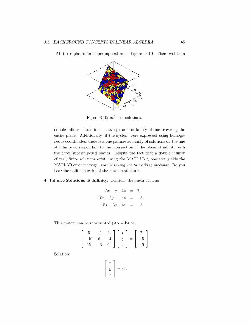
All three planes are superimposed as in Figure 3.10. There will be a

Figure 3.10: ∞2 real solutions.

double infinty of solutions: a two parameter family of lines covering the

entire plane. Additionally, if the system were expressed using homoge-

neous coordinates, there is a one parameter family of solutions on the line

at infinity corresponding to the intersection of the plane at infinity with

the three superimposed planes. Despite the fact that a double infinity

of real, finite solutions exist, using the MATLAB \ operator yields the

MATLAB error message: matrix is singular to working precision. Do you

hear the polite chuckles of the mathematicians?

4: Infinite Solutions at Infinity. Consider the linear system:

5x− y + 2z = 7,

−10x+ 2y +−4z = −5,

15x− 3y + 6z = −5.


−10 6 −4

15 −3 6

x

y

z

=

7

−5

−5

.Solution: x

y

z

=∞.


Figure 3.11: One solution where the line at infinity of two of the planes intersects

the third plane.

The three equations represent three parallel non-coincident planes, as in

Figure 3.11. When represented using homogeneous coordinates, the three

planes all intersect the plane at infinity in the same real, but non finite

line: a unique line on the plane at infinity.

5: No Finite, But One Infinite Solution. Consider the linear system:

5x− y + 2z = 7,

−2x+ 6y + 9z = 0,

−10x+ 2y − 4z = 18.


−2 6 9

−10 2 −4

x

y

z

=

7

0

18

.Solution:

5x− y + 2z = 7,

5x− y + 2z = −9.

In this system, there are two parallel (linearly dependent, but not coinci-

dent) planes, intersecting a third plane as in Figure 3.12. There will never

be a finite point/line/plane where the system of equations will intersect.

But, it can be seen that the two parallel planes intersect the third in two

distinct parallel lines. These two parallel lines intersect in a unique point

at infinity.


Figure 3.12: Lines of intersection of each pair of planes are parallel, meaning

one unique solution at infinity. plane.

6: No Finite, But One Infinite Solution. Consider the linear system:

5x− y + 2z = −12,

−2x+ 6y + 9z = 0,

8y + 14z = 8.


−2 6 9

0 8 14

x

y

z

=

−12

0

8

,Solution: three parallel lines. Each pair of the three planes intersect in a

distinct line, as shown in Figure 3.13. The line of intersection of each pair

of planes is parallel to the third. The parallel lines intersect in a single

real point at infinity.

Figure 3.13: No Finite Solution: three planes intersecting in three non-

intersecting lines.


3.1.5 Linear Least-Squares Problem

In a system of linear equations Am×nx = b, when there are more equations

than unknowns, m > n, and the set is said to be over-determined, there is, in

general, no solution vector x. The next best thing to an exact solution is the best

approximate solution. This is the solution that comes closest to satisfying all the

equations simultaneously. If closeness is defined in the least-squares sense, then

the sum of the squares of the differences between the left- and right-hand sides

of Am×nx = b must be minimised. Then the over-determined linear problem

becomes a (usually) solvable linear problem: the linear least-squares problem.

This concept will be employed extensively starting in Section 3.4.1.

Generally, we start with an optimality condition called the normality condi-

tion. Conceptually, we can transform the m× n system to an n× n system by

pre-multiplying both sides by AT :

(ATn×mAm×n)xn×1 = AT

n×mbm×1.

These are typically referred to as the normal equations of the linear least-squares

problem. Direct solution of the over-determined system of equations relies on

the Moore-Penrose generalised inverse [4] (M-PGI) of the rectangular matrix

A, which yields:

xn×1 ≈ (ATn×mAm×n)−1AT

n×mbm×1.

The quantity (ATn×mAm×n)−1AT

n×m is the M-PGI.

It turns out that singular value decomposition can solve the normal equa-

tions, using householder reflections, without explicitly evaluating them, see Sec-

tions 3.1.8 and 3.1.9. It is always worth repeating that direct solution of the

normal equations is usually the worst way to find least-squares solutions because

of numerical conditioning, see Section 3.1.7, and indirect methods of approxi-

mating the best compromise solution relative to some index should be employed,

such as Householder reflections, or singular value decomposition. Using the M-

PGI to approximate a solution is termed the naıve approach.

In summary, given an objective function z = (1/2)eTe to minimise over x,

in an over-determined set of equations, we have

The Normality Condition:∂z

∂x= 0;

The Normal Equations:

(ATA)x−ATb = 0;


The Naıve Solution:

x = (ATA)−1ATb.

In what follows we discuss why using the M-PGI is considered naıve and what

can be used in its place.

3.1.6 Nullspace, Range, Rank:

The nullspace, range, rank, and nullity are measures of capability of linear

mappings in the form of vector-matrix equations that will help us avoid using

the naıve approach to solving the system of equations outlined above to solve

systems of linear equations. Consider the following linear system as a mapping

Ax = b.

Matrix A may be viewed as a map from the vector space x to the vector space

b.

Nullspace: The nullspace of A is a subspace of x that A maps to 0. It is the

set of all linearly independent x that satisfy

Ax = 0.

The dimension of the nullspace is called the nullity of A.

Range: The range of A is the subspace of b that can be reached by A for the

x not in the nullspace of A

Rank: The dimension of the range is called the rank of A. For an n × n

square matrix, rank+nulity = n. For a non-singular n×n square matrix

rank(A) = n.

The maximum effective rank of a rectangular m× n matrix is the rank of

the largest square sub-matrix. For m > n, full rank means rank(A) = n

and rank deficiency means rank < n

3.1.7 Numerical Conditioning

The condition number of a matrix is a measure of how invertible or how close

to singular a matrix is. The condition number of a matrix is the ratio of the

largest to the smallest singular values.

k(A) =σmax

σmin.


A matrix is singular if k =∞, and is ill-conditioned if k is very large. But, how

big is large? Relative to what? The condition number is lower bounded by a

finite number, but the upper bound is infinite

1 ≤ k(A) ≤ ∞.

Instead, let’s consider the reciprocal of k(A). Let this reciprocal be λ(A) such

that

λ(A) = 1/k(A).

This ratio is bounded both from above and below

0 ≤ λ(A) ≤ 1.

Now we can say A is well-conditioned if λ(A) ' 1, and ill-conditioned if λ(A) '0. But, now how small is too close to zero. Well, this we can state with certainty.

A numerical value for too small is the computer’s floating-point precision which

is typically 10−12 for double precision computations. MATLAB uses double

floating-point precision for all computations. Hence, if λ(A) < 10−12, A is

ill-conditioned.

3.1.8 Householder Reflections

We will generally want to avoid using the naıve approach to solving the system

of equations outlined in Section 3.1.5, and adopt an approach that is insensitive

to the conditioning of the equations. Consider the matrix equation

Am×nxn×1 = bm×1.

The least-squares solution to a suitably large over-determined system involves

the pseudo, or Moore-Penrose generalized inverse of A. Given A and b, we can

approximate x in a least-squares sense as:

x ≈ (ATA)−1ATb. (3.4)

Practically, however, if A has full rank, then Householder reflections [9] (HR),

also known as Householder transformations, are employed to transform A and

b. They represent a change of basis that do not change the relative angles

between the basis column vectors of A. An HR is a linear transformation that

describes a reflection about a plane or hyperplane containing the origin. Hence,

they are proper isometries that do not distort the metric on either A or b. The

ith HR is defined such that

HTi Hi = I, and det(Hi) = −1.


Thus, Hi is orthogonal, but not necessarily symmetric. The dimensions of the

system of original equations are illustrated in Figure 3.14. For the dimensions

Figure 3.14: Dimensions of the system of linear equations.

of an m×n matrix A and an m× 1 vector b, n HR’s are required to transform

A and b. Each HR is an m×m matrix that transforms the system into a set of

n canonical equations, as illustrated in Figure 3.15, which allows the unknown

elements of x to be solved for using back-substitution. It is important to re-

Figure 3.15: Visualisation of how the Householder reflections transform the

m× n equations into a set of n canonical equations.

member that when coding an algorithmic based piece of software for designing

optimised linkages that it is typically not a good choice to blindly use the pseudo

inverse to approximate x, but Householder reflections instead when A has full

rank. What if A does not possess full rank, or worse, possesses full rank but

with a very large condition number? This is where SVD can be used. It is

much more than the flavor-of-the-month least-squares numerical approximation

algorithm. It is a very powerful technique for dealing with sets of equations that

are either singular (contain linear dependencies), numerically close to singular,

or even fully determined and well constrained.


3.1.9 Singular Value Decomposition (SVD)

Singular value decomposition (SVD) is a powerful technique for dealing with

sets of equations that are either singular, or numerically close to singular. In

many cases where Gaussian elimination, Householder reflections, or the M-PGI

fail to yield useful results, SVD will diagnose exactly what the cause of problem

is, and determine a useful numerical solution. This is a result of the fact that

SVD explicitly constructs orthonormal bases for both the nullspace and range

of every matrix A.

SVD is based on the fact that every m× n matrix A, square or rectangular

of any dimension, can be decomposed into the product of the following matrix

factors:

Am×n =

{Um×nΣn×nVT

n×n called the economy size version[10],

Um×mΣm×nVTn×n called the full size version,

where for the economy size version, which we will use:

• Um×n is column-orthonormal, the column vectors are all mutually orthog-

onal unit vectors. In other words, using MATLAB syntax

U(:, j) ·U(:, k) =

{1 if j = k

0 if j 6= k

• Σn×n is a diagonal matrix whose diagonal elements are the singular values,

σi of A. The singular values of A are the square roots of the eigenvalues

of ATA. They are positive numbers arranged in descending order lower

bounded by zero. The eigenvalues are obtained by solving the character-

istic equation of A which is obtained from

(ATA)x = λx⇒ (ATA− λI)x = 0.

The corresponding characteristic equation is

ATA− λI = 0.

Solving this system of equations for all values of λ reveals the singular

values of A:

σi =√λi.

• V is a square orthogonal matrix, i.e. both it’s columns and rows are

orthonormal, so

VVT = I.


These important properties mean that the inverses of U, Σ, and V are

trivial to compute. Because U and V are orthogonal their inverses are equal to

their transposes. Because Σ is diagonal, it’s inverse is another diagonal matrix

whose elements are the reciprocals of the elements σi. The only thing that can

go wrong is for one of the σi to be zero, or for it to be so small that it’s numerical

value is dominated by roundoff error and therefore unknowable.

Recall that for an m×n matrix A, where m > n, to possess full rank means

that rank = n. In this case, all σi, i = 1...n, are positive, non-zero real numbers.

The matrix is (analytically) non-singular. If A is rank deficient then some of

the σi are identically zero. The number of σi = 0 corresponds to the dimension

of the nullspace (n − rank(A)). The σi are arranged in Σ on the diagonal in

descending order: σ1 ≥ σ2, σ2 ≥ σ − 3, ... , σn−1 ≥ σn

• The columns of U whose same-numbered elements σi are non-zero are

an orthogonal set of orthonormal basis vectors that span the range of A:

every possible product Ax = b is a linear combination of these column

vectors of U.

• The columns of V whose same numbered elements σi = 0 form an orthog-

onal set of orthonormal basis vectors that span the nullspace of A: every

possible product Ax = 0 is a linear combination of these column vectors

of V, see Figure 3.16.

Figure 3.16: Visualisation of the economy size singular value decomposition.


MATLAB Note: To get the form of SVD in Figure 3.16, the syntax is

[U,S,V] = svd(A, 0).

For any matrix Am×n, the MATLAB command svd(A,0) returns the three

matrices Um×n, Sn×n (the singular values), and Vn×n such that A = USVT .

Note that the matrix S is equivalent to the matrix Σ described earlier.

What computational advantage does this provide? Every matrix, no matter

how singular, can be inverted! By virtue of the properties of U, Σ, and V, the

inverse of any matrix A, square or not, is simply

A−1 = (Um×nΣn×nVTn×n)−1 = Vn×nΣ−1n×nUT

n×m.

Because V and U are orthogonal their inverses are equal to their transposes.

Because Σ is diagonal its inverse, Σ−1, has elements 1/σi on the diagonal and

zeroes everywhere else. So we can write explicitly:

A−1n×m = Vn×n[diag(1/σi)]UTn×m.

Computational problems can only be caused if any σi = 0, or are so close to

zero that the value of σi is dominated by roundoff error so that 1/σi becomes a

very large, but equally inaccurate number, which pushes A−1 towards infinity

in the wrong direction. That doesn’t bode well for the solution x = A−1b.

3.1.10 What to do When A is Singular

When matrix A is non-singular and square, then it maps one vector space onto

one of the same dimension. For the m × n case x is mapped onto b so that

Ax = b is satisfied but the dimensions of x and b are different, see Figure 3.17.

However, if A is singular we can still find a useful solution. A more detailed

discussion of the material in this section may be found in the book Numerical

Recipes in C [10]. There are three cases to consider if k(A) =∞.

1. If b = 0, the solution for x is any column of V whose corresponding

σi = 0. This is so because for a non-trivial solution to exist for the system

Ax = 0 then at least one σi = 0 because the determinant of A must be 0.

2. If b 6= 0 the important question is if there exist any x that can be reached

by A, in other words, is b in the range of A? If b is in the range of A,

but A is singular then the set of equations does have a solution x, in fact

it has infinitely many. Any vector in the nullspace, i.e., any column of V


with a corresponding zero σi, can be added to x in any linear combination.

This is graphically illustrated in Figure 3.18.

But this is where things get really interesting. The x with the smallest

Euclidean norm can be obtained by setting ∞ = 0!! This, however, is not

the desperation mathematic is appears to be at first glance. If σi = 0, set

(1/σi) = 1/0 = 0 in Σ−1. Then, the x with the smallest 2-norm is

x = V[diag(1/σi)](UTb), i = 1, ..., n. (3.5)

Where for all σi = 0, 1/σi is set to zero. (Note, in Figure 3.18 the equation

Ax = d is used for this case.)

3. If b 6= 0 but is not in the range of A (this is typical in over-determined

systems of equations). In this case the set of equations are inconsistent,

and no solution exists that simultaneously satisfies them. We can still

use Equation (3.5) to construct a solution vector x that is the closest

approximation in a least-squares sense. In other words, SVD finds the x

that minimises the norm of the residual r of the solution, where

r ≡ ||Ax− b||2.

Referring to Equation (3.11), note the happy similarity to the design error!!

This is illustrated in Figure 3.18.

Figure 3.17: Matrix A is non-singular and maps one vector space onto one of

the same dimension if A is square. For the m × n case x is mapped onto b so

that Ax = b is satisfied but the dimensions of x and b are different.


Figure 3.18: Matrix A is singular. If A is square it maps a vector space of

lower dimension (in the figure A maps a plane onto a line, the range of A).

The nullspace of A maps to zero. The “solution” vector x of Ax = d consist

of a particular solution plus any vector in the nullspace. In this example, these

solutions form a line parallel to the nullspace. SVD finds the x closest to zero

by setting 1/σi = 0 for all σi = 0. Similar statements hold for rectangular A.

3.2 Numerical Reality

Thus far we have presumes that either a matrix is singular or not. From an

analytic standpoint this is true, but not numerically. It is quite common for

some σi to be very, very small, but not zero. Analytically the matrix is not

singular, but numerically it is ill-conditioned. In this case Gaussian elimination,

or the normal equations will yield a solution, but one when multiplied by A very

poorly approximates b.

The solution vector x obtained by zeroing the small σi and then using equa-

tion (3.5) usually gives a better approximation than direct methods and the

SVD solution where small σi are not zeroed.

Small σi are dominated by, and hence are an artifact of, roundoff error. But

again we must ask “How small is too small?”. A plausible answer is to edit

(1/σ− i) if (σi/σmax) < µε where µ is a constant and ε is the machine precision.

MATLAB will tell you what ε is on your machine: in the command window,

type eps followed by pressing enter. On my desktop ε = 2.2204 × 10−16. It

turns out that a useful value for µ is rank(V ). So we can state the following,

easy rule for editing 1/σi:

set 1/σ − i = 0 if (σi/σmax) < rank(V)ε.

At first it may seem that zeroing the reciprocal of a singular value makes a bad

situation worse by eliminating one linear combination of the set of equations we

3.3. KINEMATIC SYNTHESIS 77

are attempting to solve. But we are really eliminating a linear combination of

equations that is so corrupted by roundoff error that it is, at best, useless. In

fact, worse than useless because it pushes the solution vector towards infinity in

a direction parallel to a nullspace vector. This makes the roundoff error worse

by inflating the residual r = ||Ax− b||2.

In general the matrix Σ will not be singular and no σi will have to be

eliminated, unless there are column degeneracies in A (near linear combinations

of the columns). The ith column in V corresponding to the annihilated σi gives

the linear combination of the elements of x that are ill-determined even by the

over-determined set of equations. These elements of x are insensitive to the

data, and should not be trusted.

3.3 Kinematic Synthesis

The design of a device to achieve a desired motion involves three distinct synthe-

sis problems: type, number, and dimensional synthesis. These three problems

will be individually discussed in the following three subsections.

3.3.1 Type Synthesis

Machines and mechanisms involve assemblies made from six basic types of

mechanical components. These components were identified by the German

kinematician Franz Reuleaux in his classic book from 1875 Theroetische Kine-

matik [11], translated into English in 1876 by Alexander Blackie William Kennedy

(of Aronhold-Kennedy Theorem fame) as Kinematics of Machines [12]. The six

categories are:

1. eye-bar type link (the lower pairs);

2. wheels, including gears;

3. cams in their many forms;

4. the screw, which transmits force and motion;

5. intermittent-motion devices, such as rachets;

6. tension-compression parts with one-way rigidity such as belts, chains, and

hydraulic or pneumatic lines.

The selection of the type of mechanism needed to perform a specified motion

depends to a great extent on design factors such as manufacturing processes,


materials, safety, reliability, space, and economics, which are arguably outside

the field of kinematics.

Figure 3.19: There are 16 distinct ways to make a planar four-bar using only R-

and P -pairs taken 4 at a time, but only the extreme cases RRRR and PPPP

are shown.

Even if the decision is made to use a planar four-bar mechanism, the type

issue is not laid to rest. There remains the question: “what type of four-bar?”.

Should it be an RRRR? An RRRP? An RPPR? There can be 16 possible

planar chains comprising R- and P -pairs. Any one of the four links joined by

the four joints can be the fixed link, each resulting in a different motion, see

Figure 3.19 for example.

3.3.2 Number Synthesis

Number synthesis is the second step in the process of mechanism design. It

deals with determining the number of DOF and the number of links and joints

required, see Figure 3.20. If each DOF of the linkage is to be controlled in a

Figure 3.20: Linkages with 0, 1, and 2 DOF, requiring 0, 1, and 2 inputs to

control each DOF.


closed kinematic chain, then an equal number of active inputs is required. If the

linkage is a closed chain with 2 DOF then actuators are required at two joints.

If more actuators are used the device is redundantly actuated, if less are used,

the device is under actuated with uncontrolled DOF.

Open kinematic chains require that each joint be actuated. A 7R planar

open chain, as in Figure 3.21, has 3 DOF, but requires 7 actuators to control

the 3 DOF, although it is still said to be redundantly actuated. Note that in

Figure 3.21: Planar 7R with 3 DOF, even though CGK says 7 DOF.

the 7R open planar chain example, the CGK formula predicts 7 DOF:

3(8− 1)− 7(2) = 21− 14 = 7 DOF,

6(8− 1)− 7(5) = 42− 35 = 7 DOF.

The 7 DOF in E2 and E3 are indeed real, but linearly coupled. There is a

maximum of 3 DOF in the plane, and a maximum of 6 DOF in Euclidean

space.

3.3.3 Dimensional Synthesis

The third step in mechanism design is dimensional synthesis. We will con-

sider three distinct problem classes in dimensional synthesis mentioned earlier,

namely: function generation; rigid body guidance; and trajectory generation.

3.3.4 Function Generation

Dimensional synthesis boils down to solving a system of synthesis equations

that express the desired motion in terms of the required unknown dimensions.

These unknowns include, among other things, the link lengths, relative locations


Figure 3.22: Elements of the Freudenstein parameters for a planar 4R linkage.

of revolute centers, and in particular for function generators, a zero or home

configuration.

3.3.5 Dimensional Synthesis Continued

The synthesis equations for a four-bar function generator that are currently

used were developed by Ferdinand Freudenstein in his Ph.D thesis in 1954, and

published one year later [13]. Consider the mechanism in the Figure 3.22. The

Freudenstein parameters, k1, k2, and k3 are the link length ratios:

k1 ≡ (a21 + a22 + a24 − a23)

2a2a4,

k2 ≡ a1a2,

k3 ≡ a1a4.

⇔

a1 = 1,

a2 =1

k2,

a4 =1

k3,

a3 = (a21 + a22 + a24 − 2a2a4k1)1/2.

(3.6)

The ith configuration of the linkage illustrated in Figure 3.22 is governed by

the following synthesis equation:

k1 + k2 cos(ϕi)− k3 cos(ψi) = cos(ψi − ϕi). (3.7)

Three distinct sets of input and output angles (ψ,ϕ) define a fully determined

set of synthesis equations, implying that if there is a solution for k1, k2, k3 that

satisfies the three equations, it will be unique. Thus, we can determine the link


length ratios (k1, k2, k3) that will exactly satisfy the desired function ϕ = f(ψ).

Of course for a function generator we only require ratios of the links because

the scale of the mechanism is irrelevant. We will find it helpful to express a set

of three, or more, synthesis equations in vector-matrix form, defined shortly in

Section 3.4.

What happens if you need a function generator to be exact over a continuous

range of motion of the mechanism? Sadly, you can’t have it. A solution, in gen-

eral, does not exist! Now do you hear the somewhat more enthusiastic chuckles

of the mathematicians? To be exact, greater than three prescribed configura-

tions results in an over-determined system (more equations than unknowns),

which in general has no solution. We could try to make an improvement by

formulating the problem so that there were more unknowns. Recall the steering

condition, reproduced here:

S(∆ψ∆ϕ) ≡ sin(∆ϕ−∆ψ)− ρ sin(∆ψ) sin(∆ϕ) = 0. (3.8)

Define the dial zeroes to be α and β such that:

ψi = α+ ∆ψi,

ϕi = β + ∆ϕi, (3.9)

The synthesis equation now becomes:

k1 + k2 cos(β + ∆ϕi)− k3 cos(α+ ∆ψi) = cos ((α+ ∆ψi)− (β + ∆ϕi)) .(3.10)

Now five sets of (∆ψi,∆ϕi) will produce five equations in five unknowns. This

means that the function will be generated exactly for five inputs only. There is

no guarantee about the values in between the precision input-output values of

the function. If this was how steering linkages were designed we would wear out

our tires very fast, and have difficulty cornering.

Note, the design constant ρ must be selected, where ρ = b/a, with b =

track (distance between wheel carrier revolutes), and a = wheelbase (distance

between axle center-lines). A typical value for a car is ρ = 0.5. We will use this

value in the following example shown in Figure 3.23. To resolve the problem,

we resort to approximate synthesis, instead of exact synthesis. This involves

over-constraining the synthesis equation. We generate a set of m equations in

n unknowns with m� n. In our case n = 5. Two questions immediately arise:

What value should be given to m? Moreover, how should the input data be

distributed? The answer to both questions depends on context, and usually

requires some experimentation.


Figure 3.23: The steering condition, Figure 3.4 reproduced here for easy refer-

ence.

Assuming we have selected m and a distribution for the m input-output

(I/O) values, we want a solution that will generate the function with the least

error. The design and structural errors are two performance indicators used to

optimise approximate synthesis.

3.4 Design Error

Given an over-constrained system of linear equations, an over-abundance of

equations compared to unknowns, in general the system is inconsistent. If dial

zeroes α and β have been determined, then we have the three unknown Freuden-

stein parameters [k1, k2, k3]T = k that must satisfy the m� 3 equations. Since,

in general, no vector of Freudenstein parameters k can satisfy all the synthesis

equations exactly and the product of the synthesis matrix with the Freudenstein

parameter vector does not equal the vector whose elements are the cosine of the

differences of the prescribed input and output angles, or Sk 6= b. Hence, the

design error d is defined as:

d = b− Sk, (3.11)

3.4. DESIGN ERROR 83

where for the m equations S is an m× 3 matrix called the synthesis matrix

S =

1 cos(ϕ1) − cos(ψ1)

1 cos(ϕ2) − cos(ψ2)...

......

1 cos(ϕm) − cos(ψm)

,and b is the m× 1 vector

b =

cos(ψ1 − ϕ1)

cos(ψ2 − ϕ2)...

cos(ψm − ϕm)

. (3.12)

k is the 3× 1 vector of unknown Freudenstein parameters, and d is the m× 1

design error vector. The Euclidean norm of d is a measure of how well the

computed k satisfies the vector equation

Sk = b.

Clearly, if m = 3 and S is non-singular and square then

k = S−1b.

For m > 3 we can only approximate a solution for k using a linear least

squares approach. This means that we require some form objective function to

optimise. For the design error, the objective function is defined to be

z = (1/2)(dTWd), (3.13)

which must be minimised over k. The quantity (dTWd)1/2 is the weighted

Euclidean norm, while dTWd is the weighted Euclidean innerproduct. This

requires a few words of explanation.

The matrix W is a diagonal matrix of positive weighting factors. They are

used to make certain data points affect the minimisation more, or less, than

others depending on their relative importance to the design. We usually start

by setting W = I (the identity matrix).

3.4.1 Minimising the Design Error

We are now in a position to resume examining the objective function for min-

imising d over k:

z = (1/2)d TWd.


Typically, one half of the square of the weighted 2-norm is used. The weighted

2-norm of d over k can be minimised, in a least-squares sense by transforming S

using Householder reflections which were discussed in Section 3.1.8, or singular

value decomposition (SVD), discussed in Section 3.1.9.

Briefly, in MATLAB householder orthogonalization is invoked when a rect-

angular matrix is divided by a vector, using the syntax

k = S \ b.

Be warned that this symbolic matrix division is literally symbolic: the operation

does not exist in a vector space! The backslash operator invokes an algorithm

that employs Householder orthogonalization of the matrix. Using SVD is some-

what more involved, but information on how well each element of k has been

estimated is a direct, and extremely useful output of the decomposition.

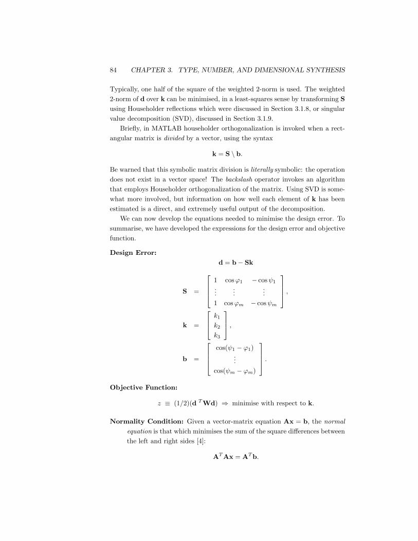
We can now develop the equations needed to minimise the design error. To

summarise, we have developed the expressions for the design error and objective

function.

Design Error:

d = b− Sk

S =

1 cosϕ1 − cosψ1

......

...

1 cosϕm − cosψm

,

k =

k1

k2

k3

,

b =

cos(ψ1 − ϕ1)

...

cos(ψm − ϕm)

.Objective Function:

z ≡ (1/2)(d TWd) ⇒ minimise with respect to k.

Normality Condition: Given a vector-matrix equation Ax = b, the normal

equation is that which minimises the sum of the square differences between

the left and right sides [4]:

ATAx = ATb.

3.4. DESIGN ERROR 85

We start by imposing the condition that

dz

dk= 0 ⇒

∂z/∂k1

∂z/∂k2

∂z/∂k3

= 0,

which is called the normality condition. Next, we wish to express the

normality condition in terms of the synthesis equations. Using the chain

rule we see the normality condition possesses the form:

dz

dk⇒ dz

dki=

dz

ddj

ddjdki

⇒ dz

dk=

(dd

dk

)Tdz

dd.

From this, it is to be seen that(dd

dk

)T= −ST , and

dz

dd= Wd.

Therefore, the normality condition can be expressed as

dz

dk= −STWd = −STW(b− Sk) = 0.

Finally, from the normality condition we see that the normal equations

possess the form that the definition requires:

−STWb+STWSk = 0 ⇒ (STWS)(3×3)k(3×1) = (STW)(3×m)b(m×1).

Because W is positive definite then STi WSi > 0 and the k obtained, at

least conceptually, are the optimal k that minimise the objective function

z, and we can state that

kopt = (STWS)−1STWb.

The term (STWS)−1STW in the above equation is called the weighted

Moore-Penrose Generalized Inverse (M-PGI) of S.

Calculating the M-PGI conceptually leads to kopt, however, this is generally

not the case numerically when m� n because (STWS)−1STW is typically ill-

conditioned, meaning that the ratio of the associated maximum and minimum

singular values of STWS is very large:

σmaxσmin

≈ ∞ because σmax � σmin.


The norm of the optimal solution vector, kopt, obtained using the M-PGI is in

general so corrupted by round-off error that it is, at best, useless.

We should resort to a numerical approximation that is insensitive to the

conditioning of the M-PGI of S. Geometrically, we must find k whose image

under S is as close as possible to b, see Figure 3.24. What the figure illustrates

is that the left and right hand sides of the synthesis equation can be represented

as vector magnitudes both originating at the point 0. Different magnitudes for

k effectively rotate Sk about 0 in the plane. The distance between Sk and b

is d. Certainly, kopt yields dmin. This implies that Householder Reflections,

described in Section 3.1.8, or some other numerical method should be used to

identify kopt.

Figure 3.24: The optimal Freudenstein parameters, kopt, yields smallest differ-

ence, dmin, between Sk and b.

3.5 Structural Error

The structural error is defined to be the difference between the prescribed and

generated output angle values for a given input angle value. From a design

optimisation perspective, it could be argued that the structural error is a better

performance indicator than the design error in the sense that it directly measures

the performance of the mechanism, while the design error is an algebraic residual

created by any difference between Sk and b for identified values of k which

minimise an objective function. However, in [14] it has been observed that as

the cardinality of the prescribed discrete input-output (I/O) data-set increases,

the corresponding linkages that minimise the Euclidean norms of the design

and structural errors tend to converge to the same linkage. The important

3.5. STRUCTURAL ERROR 87

implication of this observation is that the minimisation of the Euclidean norm

of the structural error can be accomplished indirectly via the minimisation of the

corresponding norm of the design error, provided that a suitably large number

of I/O pairs is prescribed.

The importance arises from the fact that the minimisation of the Euclidean

norm of the design error leads to a linear least-squares problem whose solution

can be obtained directly as opposed to iteratively [4], while the minimisation of

the same norm of the structural error leads to a nonlinear least-squares problem,

and hence, calls for an iterative solution [15]. Working with the observation

reported in [14], an effort has been initiated to extend the discrete approximate

synthesis problem into a continuous one by integrating the synthesis equations

in the range of minimum input angle to maximum input angle and minimising

the design error [16]. Currently, minimising the structural error in the context

of continuous approximate synthesis is an open problem. The solution of this

problem is an important challenge because it could stand to prove, or disprove

the observation in [14].

Let the structural error vector s be defined as

s ≡ [ϕpres,i − ϕgen,i], i ∈ 1, 2, ..,m.

To minimise the Euclidean, or 2-Norm, of s requires an iterative numerical

procedure. The scalar objective function to be minimised over k is

ζ = (1/2)(sTWs).

Here, again W is an m×m diagonal matrix of weighting factors.

Minimising the norm of the structural error s is a non-linear problem. One

way to proceed is to use the Gauss-Newton procedure, using the Freudenstein

parameters that minimise the Euclidean norm of the design error as an initial

guess. The guess is modified until the normality condition, which is the gradient

of ζ with respect to k, is satisfied to a specified tolerance. For exact synthesis

the normality condition must be identically satisfied as

∂ζ

∂k= 0.

Setting W = I for representational simplicity, the objective function reduces to

ζ =1

2sT s, which is essentially

1

2||s||22.

We wish to minimise this error over the Freudenstein parameter vector k.


From the normality condition we can write

∂ζ

∂k=

(∂s

∂k

)T3×m

∂ζ

∂sm×1. (3.14)

It is to be seen that∂ζ

∂s= s,

and that∂s

∂k=

∂

∂k(ϕpres −ϕgen).

Since the prescribed output angle values are constant, by definition, we have

∂ϕpres∂k

= 0,

which, in turn, implies that

∂s

∂k= −

∂ϕgen∂k

.

Recall that the synthesis equations are Sk − b = 0 for an ideal function

generator. It will be convenient to express these equations as a function of the

generated output angles, the Freudenstein parameters, and the input angles:

Sk− b = f(ϕgen,k;ψ) = 0. (3.15)

For m input angles we will obtain m values for the function:

ψ =

ψ1

...

ψm

,

f =

f1...

fm

.If the derivative of f with respect to k is identically equal to 0, then the total

derivative of f with respect to k can be written as the sum of the partials:

df

dk=

(∂f

∂k

)m×3

+

(∂f

∂ϕgen

)m×m

(∂ϕgen∂k

)m×3

= 0m×3. (3.16)

As was just shown, the last partial in Equation 3.16 is

∂ϕgen∂k

= − ∂s

∂k,


because the prescribed values of the output angles are constant with respect to

differentiation. The middle partial derivative of f with respect to ϕgen is an

m×m diagonal matrix:

∂f

∂ϕgen= diag

(∂f1

∂ϕgen,1, · · · , ∂fm

∂ϕgen,m

)≡ D.

Since we assume that Equation (3.16) is identically zero, we have

∂f

∂ϕgen

∂ϕgen∂k

= − ∂f

∂k.

Rearranging gives:

∂ϕgen∂k

= −D−1∂f

∂k. (3.17)

Since f is linear in k

∂f

∂k= S.

All of the above relations can be used to rewrite Equation (3.17) as:

∂s

∂k= −(−D−1S) = D−1S. (3.18)

Substituting Equation (3.18) into Equation (3.14) yields

∂ζ

∂k=(D−1S

)Ts = STD−1s = 0. (3.19)

The Euclidean norm of the structural error s attains a minimum value when

D−1s lies in the nullspace of ST . From Equation (3.15) we can write:

ϕgen = ϕgen(k),

but we want

ϕgen(k) = ϕpres.

Assume we have an estimate for kopt, which we call kυ obtained from the

υth iteration. We can introduce a correction vector ∆k so that we get

ϕgen(kυ + ∆k) = ϕpres. (3.20)

We can linearise the problem by expanding the left hand side of Equation (3.20)

in a Taylor series and ignoring the nonlinear higher order terms:

ϕgen(kυ) +∂ϕgen∂k

|kυ∆k + higher order terms = ϕpres.


Substituting the results from Equation (3.17)

∂ϕgen∂k

= −D−1S,

into the Taylor series and rearranging leads to:

D−1S∆k = ϕgen(kυ)−ϕpres = −sυ. (3.21)

Next, we can compute ∆k conceptually as the M-PGI:

∆k = −(STD−1S)−1ST sυ. (3.22)

However, in MATLAB a least squares approximation of Equation (3.22) for the

υth iteration is obtained using Householder transformations as

∆k = −D−1S \ sυ. (3.23)

The procedure stops when

||∆k|| < ε > 0,

and

∆k → 0 ⇒ STD−1sυ → 0,

which is exactly the normality condition. The procedure will converge to a

minimum ζ.

The elements of the diagonal matrix D are computed as

∂f1∂ϕgen,1

=∂

∂ϕgen,1[k1 + k2 cos(ϕgen,1)− k3 cos(ψ1)− cos(ψ1 − ϕgen,1)] ,

= −k2 sin(ϕgen,1)− sin(ψ1 − ϕgen,1).

The matrix D can then be assembled as

D =

∂f1

∂ϕgen,10 · · · 0

0 ∂f2∂ϕgen,2

· · · 0

0 0. . .

...

0 · · · 0 ∂fm∂ϕgen,m

=

d11 0 0 · · · 0

0 d22 0 · · · 0

0 0 d33 · · ·...

0 · · · 0. . . 0

0 · · · 0 0 dm

.


Conveniently, the inverse of a diagonal matrix consists of the reciprocals of the

diagonal elements, giving

D−1 =

1/d11 0 0 · · · 0

0 1/d22 0 · · · 0

0 0 1/d33 · · ·...

0 · · · 0. . . 0

0 · · · 0 0 1/dm

.

The formulation above yields the minimum structural error in a least squares

sense such that

ϕgen(k) ≈ ϕpres. (3.24)

Bibliography

[1] W. Norris. Modern Steam Road Wagons. Longmans, Green, and Co.,

London, New York, Bombay, 1906.

[2] L. Burmester. Lehrbuch der Kinematik. Arthur Felix Verlag, Leipzig, Ger-

many, 1888.

[3] J. E. Gentle. Numerical Linear Algebra for Applications in Statistics.

Springer, New York, N.Y., U.S.A., 1998.

[4] G. Dahlquist and A. Bjorck. Numerical Methods, translated from Swedish

by N. Anderson. Prentice-Hall, Inc., U.S.A., 1969.

[5] C. L. Lawson. “Contributions to the Theory of Linear Least Maximum

Approximations”. Ph.D. Thesis, UCLA, Los Angeles, Ca., U.S.A., 1961.

[6] J. R. Rice and K. H. Usow. “The Lawson Algorithm and Extensions”.

Mathematics of Computation, vol. 101: pages 341–347, December 1967.

[7] F. Angeles and J. Angeles. “Synthesis of Function-generating Linkages with

Minimax Structural Error: the Linear Case”. Proc. 13th IFToMM World

Congress, June 2011.

[8] H. Grassmann. A New Branch of Mathematics, English translation 1995

by Kannenberg, L. C. Open Court, Chicago, Ill., U.S.A., 1844.

[9] A.S. Householder. “Unitary Triangularization of a Nonsymmetric Matrix”.

Journal of the Association for Computing Machinery (JACM), vol. 5, no. 4:

pages 339–342, 1958.

[10] W.H. Press, S.A. Teukolsky, W.T. Vetterling, and B.P. Flannery. Numer-

ical Recipes in C, 2nd Edition. Cambridge University Press, Cambridge,

England, 1992.

93

94 BIBLIOGRAPHY

[11] F. Reuleaux. Theoretische kinematik: Grundzuge einer Theorie des

Maschinenwesens. Braunschweig, F. Vieweg und Sohn, 1875.

[12] F. Reuleaux. The Kinematics of Machinery: Outlines of a Theory of Ma-

chines, English translation by A.B.W. Kennedy, of Theoretische kinematik:

Grundzuge einer Theorie des Maschinenwesens. Macmillan and Company,

New York, N.Y., U.S.A., 1876.

[13] F. Freudenstein. “Approximate Synthesis of Four-Bar Linkages”. Trans.

ASME 77, pages 853-861, 1955.

[14] M.J.D. Hayes, K. Parsa, and J. Angeles. “The Effect of Data-Set Cardinal-

ity on the Design and Structural Errors of Four-Bar Function-Generators”.

Proceedings of the Tenth World Congress on the Theory of Machines and

Mechanisms, Oulu, Finland, pages 437–442, 1999.

[15] S. O. Tinubu and K. C. Gupta. “Optimal Synthesis of Function Generators

Without the Branch Defect”. ASME, J. of Mech., Trans., and Autom. in

Design, vol. 106: pages 348354, 1984.

[16] A. Guigue and M.J.D. Hayes. “Continuous Approximate Syn-

thesis of Planar Function-generators Minimising the Design Error”.

Mechanism and Machine Theory, vol. 101: pages 158–167, DOI:

10.1016/j.mechmachtheory.2016.03.012, 2016.

type, number, and dimensional synthesisfaculty.mae.carleton.ca/john_hayes/5507notes/ch3jh.pdf ·...

Documents