typicality: an improved semantic analysis galit w. sassoon...
TRANSCRIPT
Typicality: An Improved Semantic Analysis
Galit W. Sassoon, Tel Aviv University
Abstract
Parts 1-3 present and criticize Partee and Kamp’s 1995 well known
analysis of the typicality effects. The main virtue of this analysis is in the
use of supermodels, rather than fuzzy models, in order to represent
vagueness in predicate meaning. The main problem is that typicality of an
item in a predicate is represented by a value assigned by a measure
function, indicating the proportion of supervaluations in which the item
falls under the predicate. A number of issues cannot be correctly
represented by the measure function, including the typicality effects in
sharp predicates; the conjunction fallacy; the context dependency of the
typicality effects etc. In Parts 4-5, it is argued that these classical problems
are solved if the typicality ordering is taken to be the order in which
entities are learnt to be denotation members (or non-members) through
contexts and their extensions. A modified formal model is presented, which
clarifies the connections between the typicality effects, predicate meaning,
and its acquisition.
Contents:
1. What are the typicality effects?
2. The Supermodel Theory
(Partee and Kamp 1995) 2.1 Background: Multiple valued
logic in the analysis of typicality
2.2 Supermodels 2.3 The representation of typicality in
the Supermodel theory
3. Problems in The Theory 3.1 Typicality degrees of denotation members
3.2 The sub-type effect
3.3 The conjunction effect / fallacy 3.4 Partial knowledge 3.5 Numerical degrees 3.6 Prototypes
3.7 Feature sets
3.8 Conclusions of part 3
4. My Proposal: Learning Models 4.1 Learning models 4.2 The typicality ordering
4.3 Deriving degrees
4.4 Intermediate degrees of denotation members
4.5 The sub-type effect
4.6 The conjunction effect / fallacy 4.7 The negation effect
4.8 Partial knowledge 4.9 Context dependency 4.10 Typicality Features
5 What exactly do Learning
Models model? More findings 5.1 Corrections
5.2 Inferences: Indirect learning 5.3 Conclusions of part 5
6 Conclusions
Typicality: An Improved Semantic Analysis 1
1. What are the typicality effects?
Speakers order entities or sub-kinds (Dayal 2004; sub-kinds are also
called exemplars) by their typicality in predicates. For example, a robin is
often considered more typical of a bird than an ostrich or a penguin.
These ordering judgments show up in an unconcious processing effect,
namely in online categorization time: Verification time for sentences like a
robin is a bird, where subjects determine category membership for a typical
item, is faster than for sentences like an ostrich is a bird, where subjects
determine membership of an atypical item (Rosch 1973, Armstrong,
Gleitman and Gleitman 1983).
In addition, speakers consider features like feathers, small, flies and
sings, as typical of birds. Crucially, the more typical birds are more typical
in these features (Rosch 1973).
These judgments are highly context dependent. For example, within a
context of an utterance like: the bird walked across the barnyard, a chicken
is regarded as a typical bird, and categorization time is faster for the
contextually appropriate item chicken than for the normally typical but
contextually inappropriate item robin (Roth and Shoben 1983).
In addition to these basic effects, there are robust order of learning
effects. In a nutshell, typical instances are acquired earlier than atypical
ones, by children of various ages and by adults (Mervis and Rosch 1981,
Rosch 1973, Murphy and Smith 1982); in recall tasks, typical instances are
produced before atypical ones (Rosch 1973, Batting & Montague 1969);
categories are learned faster if initial exposure is to a typical member
(Mervis & Pani 1980), than if initial exposure is to an atypical member, or
even to the whole denotation in a random order; and finally, typical (or
early acquired) instances are remembered best (Heit 1997), and they affect
future learning (encoding in memory) of entities and their features (Rips
1975, Osherson et al 1990). In sum, typicality is deeply related to the order
in which instances are learnt to be members in predicate denotations.
These findings were replicated time and again (Mervis and Rosch
1981). Yet, the mental models underlying them and their relation to
predicate meaning are still a puzzle. To see this, we will now review the
well known typicality theory, which is most frequently cited by formal
semanticists, namely – The Supermodel Theory. For a more detailed
discussion of the typicality effects and other model types, see Sassoon
2005.

2 Galit Weidman Sassoon
2. The Supermodel Theory (Partee and Kamp 1995)
2.1 Background: Multiple valued logic in the analysis of typicality
Partee and Kamp's main innovation within the analysis of typicality, is in
the use of a logic with three truth values and the technique of
Supervaluations (van Fraassen 1969; Kamp 1975; Fein 1975; Veltman 1984;
Landman 1991), as opposed to the standard use of a logic with multiple truth
values (such as fuzzy logics) in the analysis of typicality in artificial
intelligence, cognitive psychology, and linguistics (Zadeh 1965; Lakoff
1973; Osherson & Smith 1981; Lakoff 1987; Aarts et al 2004).
2.1.1 Fuzzy models
In classical logics, a proposition may take as a truth value either 0 or 1. In
fuzzy logics, a proposition may take as a truth value any number in the real
interval [0,1]. For example, such a model can assume the following facts:
[1] The truth value of the proposition a robin is a bird is 1;
The truth value of the proposition a goose is a bird is 0.7;
The truth value of the proposition an ostrich is a bird is 0.5;
The truth value of the proposition a butterfly is a bird is 0.3;
The truth value of the proposition a cow is a bird is 0.1.
These values indicate the typicality degrees of the individuals or kinds
denoted by the subjects in the predicate bird.
More precisely, in such models, predicates are not associated with sets
as denotations. Rather, for every predicate P, a characteristic function,
cm(P,d), assigns to each entity d in the domain of individuals D, a value in
the real interval [0,1], its degree of membership in P. Moreover, each
predicate is associated with a prototype p, i.e. the best member possible.
Finally, a degree function cP (a distance metric) associates pairs of entities
with values in the real interval [0,1]. If, for example, r is a robin, b a blue
jay and o an ostrich, then: cP(r,b)< cP(r,o), i.e. r is more similar to b than to
o. The typicality of an entity d in P is represented as the distance of d from
the prototype of P, cP(d,p). This distance function satisfies several
constraints. For example, cP is such that any entity has zero distance from
itself (∀d∈D: cP(d,d) = 0); cP is symmetric (∀d,e∈D: cP(d,e) = cP(e,d)); and cP
has the property called the triangle inequality (∀d,e,f∈D: cP(d,e) + cP(e,f) ≥
cP(d,f)). Most important for our purposes is the monotonic decreasing relation
Typicality: An Improved Semantic Analysis 3
between d and c: The distance of entities from the prototype p of P
inversely correlates with their membership degree in P:
[2] ∀d,e∈D: (cP(d,p) ≤ cP(e,p)) → (cm(P,d) ≥ cm(P,e)).
Typicality degrees are assumed to correspond to degrees, or probabilities,
of membership in the category. This leading intuition shows up also in the
rules that predict the typicality degrees in complex predicates. There are
three composition rules for cm:
[3] 1. The complement rule for ¬: cm(¬P,d)= 1 – cm(P,d)
2. The minimal-degree rule for ∧: cm(P∧Q,d)= Min(cm(P,d),cm(Q,d))
3. The maximal-degree rule for ∨: cm(P∨Q,d)= Max(cm(P,d),cm(Q,d))
Consider, for instance, the complement rule for negated predicates in
(3.1). The degree of a goose in not-a-bird is assumed to be the complement
of its degree in bird (e.g. 1- 0.7). This rule is directly inspired by the idea that
the probability that p is the complement of the probably that not-p.
Similarly, the minimal-degree rule for conjunctions in (3.2) states that
an item’s degree in a modified noun like brown apple is the minimal degree
among the constituents, brown and apple. This rule, and other versions of
the rule for conjunctions and modified nouns in fuzzy models, are directly
inspired by the fact that the probability that p∧q cannot exceed the
probability that just p, or just q.
2.1.2 Problems of fuzzy models
Osherson and Smith 1981 have shown a variety of shortcomings of fuzzy
models. Following them, Partee and Kamp 1995 have argued at length
against such models. The main problem for these models is that they
generate wrong predictions.
Consider, for example, the-minimal-degree rule. This rule predicts that
the typicality degree of, e.g. brown-apples, cannot be bigger in brown apple
than in apple. Hence, this rule fails to predict the empirically well
established conjunction effect (Smith et al 1988) or fallacy (Tversky et al
1983), i.e. the finding that, according to speakers' intuitive judgments, both
the typicality degree (Smith et al 1988), and the likelihood of category
membership (Tversky et al 1983), of brown-apples, is bigger in brown apple
than in apple.
4 Galit Weidman Sassoon
The minimal-degree rule is most problematic when it comes to
contradictory and tautological predicates. Intuitively, the degree of all
entities in P∧¬P and P∨¬P ought to be 0 and 1, respectively. But fuzzy
models fail to predict this. For example, if a goose is a bird to degree 0.7,
then according to the complement rule, a goose is not a bird to degree 0.3.
Given this, the minimal degree rule predicts that a goose is a bird and not a
bird to degree 0.3, rather than to degree 0.
Another problem has to do with the fact that the degree function in these
models is total, though knowledge about typicality is often partial. For
example, if one bird sings and the other flies, which one is more typical? We
cannot tell out of context. This problem highlights the need for more context
dependency in the representation of typicality. Partee and Kamp 1995 have
argued at length for the importance of this aspect. Yet, we will see in part 3
that their proposal is also insufficient in this respect.
A problem which usually goes unnoticed has to do with the complement
rule. It is indeed true that the typicality orderings of negated predicates are
essentially the reverse of the orderings of the predicates that are being
negated (see, for instance, the findings reported in Smith et al 1988), yet
exceptions to this rule are quite common. Why? Because negated predicates
are often contextually restricted. For example, the set of non-birds is
frequently assumed to only consist of animals. In such contexts, non-animals
are intuitively assigned low typicality degrees both in the predicate bird and
in the negated predicate non-bird (rather than a low degree in bird and a high
degree in non-bird, as predicted by the complement rule). This judgment is
not captured because the relevant contextual factors are not represented.
2.1.3 Intermediate summary
We saw that multiple truth values, or probability degrees, as means to
indicate typicality degrees, are problematic in many respects. An alternative
theory is the Supermodel Theory (Partee and Kamp 1995). This analysis
uses the same types of mechanisms, namely – a membership degree
function cm, a prototype p, and a typicality degree function cp. However,
this analysis differs in two crucial respects. First, it replaces fuzzy logics
with three valued logics. Second, the typicality degrees are not always
coupled with the membership degrees. With these two differences, the
analysis is claimed to be significantly improved. However, while indeed
improved in some respects, we will see in part 3 that this analysis is highly
limited and problematic in other respects. In part 4 we will propose a novel

Typicality: An Improved Semantic Analysis 5
analysis which completely abandons the use of membership degree
functions, prototypes, and distance functions.
2.2 Supermodels
A supermodel M* consists of one partial model M, which I will call
'context' M. In M, denotations are only partially known. For example, the
denotation of chair in a partial context M may consist of only one item – the
prototypical chair, pchair. The denotation of non-chair may consist of only one
item too, which is very clearly not a chair, say – the prototypical sofa, psofa.
This means that in M we don't yet know if anything else, (an armchair, a
stool, a chair with less than 4 legs, a chair without a back, a chair which is not
used as a seat, a chair which is not of the normal size etc.), is a chair or not.
In addition, M is accompanied by a set T of total models (the
supervaluations in van Fraassen 1969), i.e. a set of all the possibilities seen in
M to specify the complete sets of chairs and non-chairs. In each t in T, each
item is either in the denotation of chair or in the denotation of non-chair.
Figure 1: The context structure in a supermodel M*
Formally, a supermodel M* for a set of predicates A and a set of entities D
is a tuple <M,T,m> such that:
[1] M is a partial model: Predicates are associated with partial
denotations in M, <[P]+M,[P]
-M>.
For example, if [chair]+M = {d1}, [chair]
-M = {d3}, d2 is in the
gap, we don't yet know if it is a chair or not.
[2] T is a set of total models which are completions of M:
Predicates are associated with total denotations, which are
monotonic extentions of their denotations in M:
∀t∈T, ∀P∈A:
2.1. Maximality: [P]+t ∪ [P]
-t = D (denotations are total).
2.2. Monotonicity: [P]+M ⊆ [P]
+t; [P]
-M ⊆ [P]
-t.
E.g. in each t∈T, d2 is added to [chair]+t or [chair]
-t.
tn tm
tj tk
tk ti
tr ts
M
c
6 Galit Weidman Sassoon
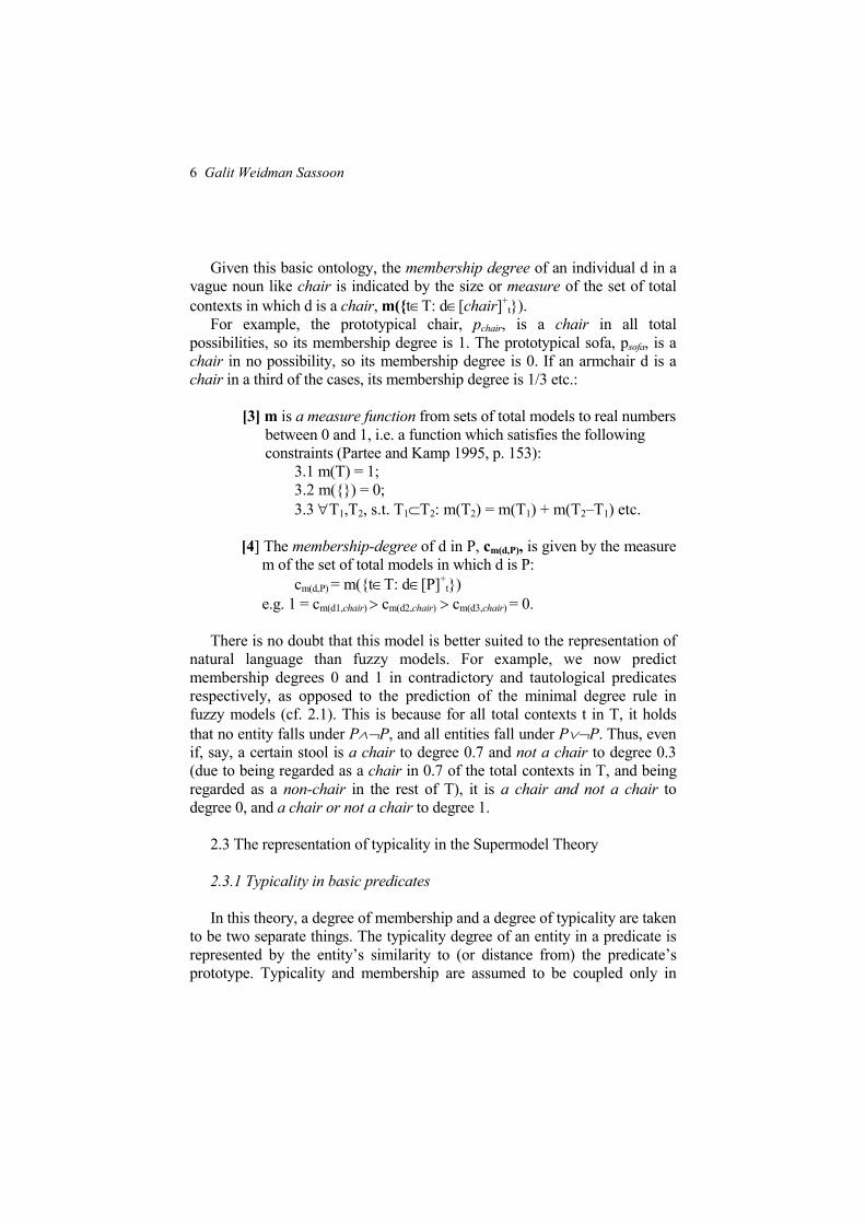
Given this basic ontology, the membership degree of an individual d in a
vague noun like chair is indicated by the size or measure of the set of total
contexts in which d is a chair, m({t∈T: d∈[chair]+t}).
For example, the prototypical chair, pchair, is a chair in all total
possibilities, so its membership degree is 1. The prototypical sofa, psofa, is a
chair in no possibility, so its membership degree is 0. If an armchair d is a
chair in a third of the cases, its membership degree is 1/3 etc.:
[3] m is a measure function from sets of total models to real numbers
between 0 and 1, i.e. a function which satisfies the following
constraints (Partee and Kamp 1995, p. 153):
3.1 m(T) = 1;
3.2 m({}) = 0;
3.3 ∀T1,T2, s.t. T1⊂T2: m(T2) = m(T1) + m(T2–T1) etc.
[4] The membership-degree of d in P, cm(d,P), is given by the measure
m of the set of total models in which d is P:
cm(d,P) = m({t∈T: d∈[P]+t})
e.g. 1 = cm(d1,chair) > cm(d2,chair) > cm(d3,chair) = 0.
There is no doubt that this model is better suited to the representation of
natural language than fuzzy models. For example, we now predict
membership degrees 0 and 1 in contradictory and tautological predicates
respectively, as opposed to the prediction of the minimal degree rule in
fuzzy models (cf. 2.1). This is because for all total contexts t in T, it holds
that no entity falls under P∧¬P, and all entities fall under P∨¬P. Thus, even
if, say, a certain stool is a chair to degree 0.7 and not a chair to degree 0.3
(due to being regarded as a chair in 0.7 of the total contexts in T, and being
regarded as a non-chair in the rest of T), it is a chair and not a chair to
degree 0, and a chair or not a chair to degree 1.
2.3 The representation of typicality in the Supermodel Theory
2.3.1 Typicality in basic predicates
In this theory, a degree of membership and a degree of typicality are taken
to be two separate things. The typicality degree of an entity in a predicate is
represented by the entity’s similarity to (or distance from) the predicate’s
prototype. Typicality and membership are assumed to be coupled only in
Typicality: An Improved Semantic Analysis 7
vague nouns like chair. In sharp nouns like bird or grandmother, they may
be dissociated. Thus:
[5] A predicate P is associated with a tuple <p, cm, cP> such that:
1. p is the prototype – the best possible P.
2. cm(d,P), is d’s membership-degree in P: the degree to which d is P.
As explained in 2.2, it is given by the measure m of the set of
total contexts in which d is a chair: cm(d,P) = m({t∈T: d∈[P]+t}.
3. cP(d,P) is d’s typicality-degree in P: d's distance from P’s
prototype.
How are the values of the typicality degree function, cP(d,P), indicated?
Generally, they are given by the values of the membership function: cP ≅ cm:
e.g. in chair: the more typical entities fall under [chair]+ in more of the total
models t in T. However, Partee and Kamp distinguish between different
predicate types in the following ways:
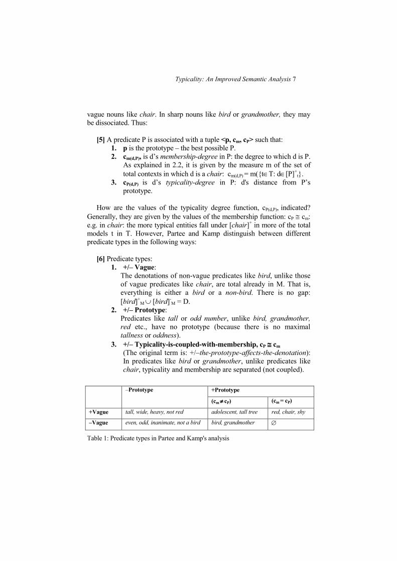
[6] Predicate types:
1. +/– Vague:
The denotations of non-vague predicates like bird, unlike those
of vague predicates like chair, are total already in M. That is,
everything is either a bird or a non-bird. There is no gap:
[bird]+M ∪ [bird]
-M = D.
2. +/– Prototype:
Predicates like tall or odd number, unlike bird, grandmother,
red etc., have no prototype (because there is no maximal
tallness or oddness).
3. +/– Typicality-is-coupled-with-membership, cP ≅≅≅≅ cm (The original term is: +/–the-prototype-affects-the-denotation):
In predicates like bird or grandmother, unlike predicates like
chair, typicality and membership are separated (not coupled).
+Prototype –Prototype
(cm ≠≠≠≠ cP) (cm = cP)
+Vague tall, wide, heavy, not red adolescent, tall tree red, chair, shy
–Vague even, odd, inanimate, not a bird bird, grandmother ∅
Table 1: Predicate types in Partee and Kamp's analysis
8 Galit Weidman Sassoon
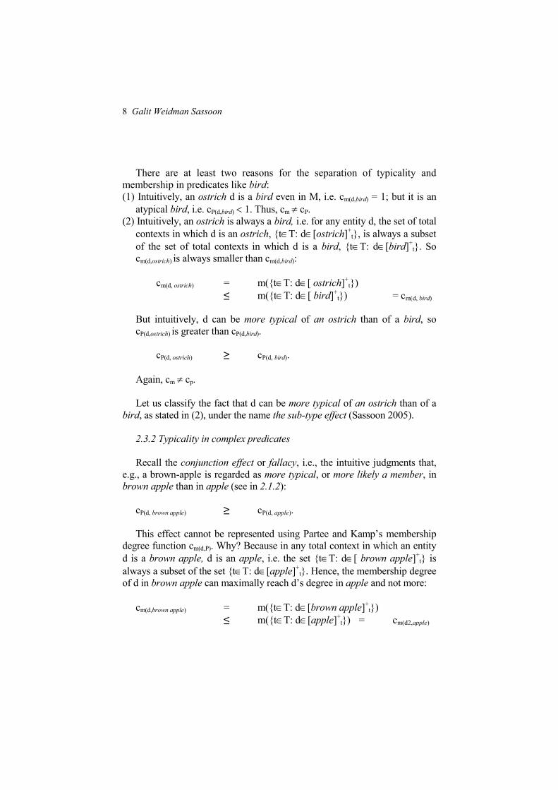
There are at least two reasons for the separation of typicality and
membership in predicates like bird:
(1) Intuitively, an ostrich d is a bird even in M, i.e. cm(d,bird) = 1; but it is an
atypical bird, i.e. cP(d,bird) < 1. Thus, cm ≠ cP.
(2) Intuitively, an ostrich is always a bird, i.e. for any entity d, the set of total
contexts in which d is an ostrich, {t∈T: d∈[ostrich]+t}, is always a subset
of the set of total contexts in which d is a bird, {t∈T: d∈[bird]+t}. So
cm(d,ostrich) is always smaller than cm(d,bird):
cm(d, ostrich) = m({t∈T: d∈[ ostrich]+t})
≤ m({t∈T: d∈[ bird]+t}) = cm(d, bird)
But intuitively, d can be more typical of an ostrich than of a bird, so
cP(d,ostrich) is greater than cP(d,bird).
cP(d, ostrich) ≥ cP(d, bird).
Again, cm ≠ cp.
Let us classify the fact that d can be more typical of an ostrich than of a
bird, as stated in (2), under the name the sub-type effect (Sassoon 2005).
2.3.2 Typicality in complex predicates
Recall the conjunction effect or fallacy, i.e., the intuitive judgments that,
e.g., a brown-apple is regarded as more typical, or more likely a member, in
brown apple than in apple (see in 2.1.2):
cP(d, brown apple) ≥ cP(d, apple).
This effect cannot be represented using Partee and Kamp’s membership
degree function cm(d,P). Why? Because in any total context in which an entity
d is a brown apple, d is an apple, i.e. the set {t∈T: d∈[ brown apple]+t} is
always a subset of the set {t∈T: d∈[apple]+t}. Hence, the membership degree
of d in brown apple can maximally reach d’s degree in apple and not more:
cm(d,brown apple) = m({t∈T: d∈[brown apple]+t})
≤ m({t∈T: d∈[apple]+t}) = cm(d2,apple)
Typicality: An Improved Semantic Analysis 9
However, Partee and Kamp observe that modifiers like brown receive a
distinct interpretation in each of the local contexts created by the noun they
modify. For example, brown is interpreted differently when applied to apple,
skin, shelf, dress etc. Thus, Partee and Kamp propose to replace cm in
modified nouns like brown apple by a new function, which may assign d a
higher value than cm(d,apple) or cm(d,brown). The modified membership function for
the modified noun brown apple, cm(d,brown /apple) is given by d’s degree in
brown, m(d,brown), minus 'a' – the minimal brown degree that the measure
function m assigns to an apple. This value is normalized by the distance
between 'a' - the minimal - and 'b' - the maximal - brown degrees assigned to
apples. This normalization procedure ensures that the result ranges between 0
and 1:
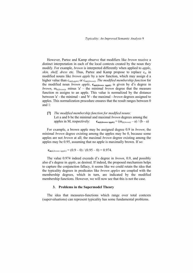
[7] The modified membership function for modified nouns:
Let a and b be the minimal and maximal brown degrees among the
apples in M, respectively: cm(d,brown /apple) = (m(d,brown) – a) / (b – a)
For example, a brown apple may be assigned degree 0.9 in brown; the
minimal brown degree existing among the apples may be 0, because some
apples are not brown at all; the maximal brown degree existing among the
apples may be 0.95, assuming that no apple is maximally brown. If so:
cm(d,brown /apple) = (0.9 – 0) / (0.95 – 0) = 0.974.
The value 0.974 indeed exceeds d’s degree in brown, 0.9, and possibly
also d’s degree in apple, as desired. If indeed, the proposed mechanism helps
to capture the conjunction fallacy, it seems like we could retain the idea that
the typicality degrees in predicates like brown apples are coupled with the
membership degrees, which in turn, are indicated by the modified
membership functions. However, we will now see that this is not the case.
3. Problems in the Supermodel Theory
The idea that measures-functions which range over total contexts
(supervaluations) can represent typicality has some fundamental problems.
10 Galit Weidman Sassoon
3.1 Typicality degrees of denotation members
The first problem has to do with the fact that the measure function m
fails to account for the fact that denotation members are not necessarily
associated with the maximal degree of typicality, 1, but rather they may
take any degree of a whole range of typicality degrees. For example, within
a certain context, I may consider three-legged seats with a back as chairs,
but as less typical chairs than four-legged seats with a back.
This limitation of the measure function is particularly problematic in
vague nouns (sharp nouns) like bird. Even atypical examples like ostriches
and penguins are known to be birds, i.e. already in M they are considered
members in [bird]+M (Partee and Kamp 1995). The bird denotations are
assumed to be completely specified, or in other words, not to vary across
different total contexts. This is the standard way in which to represent the
fact that predicates like bird are not – or are much less – vague than
predicates like chair or tall. However, this is also the reason for which the
measure function cannot indicate typicality in sharp predicates. Given that
they are always known to be birds, the membership degree of atypical
examples like ostriches and penguins in bird (i.e. the measure of the set of
total contexts in which they are birds) is always 1. And for non-birds –
whether butterflies and bats or whether stools and cows – since they are
members in [bird]-M, their membership degree in bird is always 0.
Intermediate typicality degrees in sharp nouns cannot be indicated using m.
Since no other means to indicate them is given, i.e. no general mechanism
to determine distance from the prototype is proposed, intermediate
typicality degrees in sharp nouns are not accounted for.
This is especially problematic given that the most prominent examples
of the prototype theory are indeed sharp predicates.
3.2 The sub-type effect
Furthermore, the measure function, m, fails to predict the sub-type
effect, namely, the intuition that the typicality of ostriches in ostrich
exceeds their typicality in bird. A membership degree (or measure m) is
never bigger in ostrich than in bird, because in any total context in which
an entity is an ostrich, it is also a bird (see 2.3.1). This effect is identical to
the so-called conjunction effect, but is found in lexical nouns, i.e. nouns
without a modifier, like ostrich vs. bird.
Typicality: An Improved Semantic Analysis 11
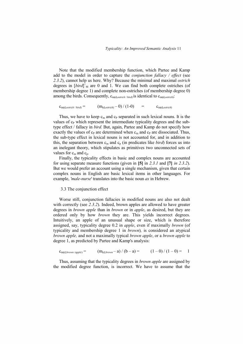
Note that the modified membership function, which Partee and Kamp
add to the model in order to capture the conjunction fallacy / effect (see
2.3.2), cannot help us here. Why? Because the minimal and maximal ostrich
degrees in [bird]+M are 0 and 1. We can find both complete ostriches (of
membership degree 1) and complete non-ostriches (of membership degree 0)
among the birds. Consequently, cm(d,ostrich / bird) is identical to cm(d,ostrich):
cm(d,ostrich / bird) = (m(d,ostrich) – 0) / (1-0) = cm(d,ostrich)
Thus, we have to keep cm and cP separated in such lexical nouns. It is the
values of cP which represent the intermediate typicality degrees and the sub-
type effect / fallacy in bird. But, again, Partee and Kamp do not specify how
exactly the values of cP are determined when cm and cP are dissociated. Thus,
the sub-type effect in lexical nouns is not accounted for, and in addition to
this, the separation between cm and cp (in predicates like bird) forces us into
an inelegant theory, which stipulates as primitives two unconnected sets of
values for cm and cp.
Finally, the typicality effects in basic and complex nouns are accounted
for using separate measure functions (given in [5] in 2.3.1 and [7] in 2.3.2).
But we would prefer an account using a single mechanism, given that certain
complex nouns in English are basic lexical items in other languages. For
example, 'male-nurse' translates into the basic noun ax in Hebrew.
3.3 The conjunction effect
Worse still, conjunction fallacies in modified nouns are also not dealt
with correctly (see 2.3.2). Indeed, brown apples are allowed to have greater
degrees in brown apple than in brown or in apple, as desired, but they are
ordered only by how brown they are. This yields incorrect degrees.
Intuitively, an apple of an unusual shape or size, which is therefore
assigned, say, typicality degree 0.2 in apple, even if maximally brown (of
typicality and membership degree 1 in brown), is considered an atypical
brown apple, and not a maximally typical brown apple, or a brown apple to
degree 1, as predicted by Partee and Kamp's analysis:
cm(d,brown /apple) = (m(d,brown – a) / (b – a) = (1 – 0) / (1 – 0) = 1
Thus, assuming that the typicality degrees in brown apple are assigned by
the modified degree function, is incorrect. We have to assume that the
12 Galit Weidman Sassoon
typicality degrees in brown apple are assigned by another mechanism. For
further empirical support to this argument, see Smith et al 1988.
There are many naturally occurring examples of utterances which refer to
typicality in complex predicates. The following examples were found in a
simple Google search on the Internet, and they contain references to
typicality in negated and/or modified nouns:
1) What were some exercises you would do on a typical non-running
day? I read that they are mainly variations of pushups and situps,
but what exactly are...
2) ... there is one week where the format will be more typical of a non-seminar class...
3) Thought it [the interview] pretty much typical of a non-fan, non-entertainment, smart up market British paper … it gives you some
sense of being there and imagine what it's like to interview a 'star'.
4) You counter with an anecdotal tale about a non-typical non-developer. How does your counter-argument apply to a typical
non-developer?
5) …her irritating non-performance is typical of a primarily young
(read 'cheap') cast…
6) The music is typical of a non-CD game - that is to say, worthless. It's tinny and very electronic sounding.
Given these examples, we cannot dismiss the problems in predicting
typicality in complex predicates on the basis that typicality is inherently
non-compositional. Though compositionality might be limited to some
extent, we need an analysis which will more correctly predict speakers'
intuitions about typicality in complex predicates when such intuitions exist.
3.4 Partial knowledge
Thus far, we have focused on problems related to the representation of the
typicality effects in sharp predicates and in complex predicates. Let us add to
this picture now another classical problem concerning the representation of
context dependency in the typicality judgments.
This problem has to do with the fact that the measure functions (or the
membership functions) are total (in every partial model M, every entity is
assigned a degree in every predicate), though knowledge about typicality is
often partial. If one bird sings and the other flies, which one is more typical?
Typicality: An Improved Semantic Analysis 13
Which bird is more typical – an ostrich or a penguin? Many contexts are too
partial to tell such facts. (Nor do speakers know every typicality feature in
every partial context. For example is in the home typical of chairs?) The
representation of knowledge about typicality needs to be more inherently
context dependent and possibly partial.
One way to do this is to define the typicality function so that it will give
each entity a value in a predicate in each total context separately (like the
interpretation function). In such a way, it would be possible that the
typicality degree of an entity (just like its membership in a predicate) is
unknown in a partial model M. It would be unknown if and only if this
entity's degree varies across different total contexts. However, note that the
measure function in Partee and Kamp 1995 is defined per supermodel (it is
a meaure of the proportion of valuations in T in which each item is a
predicate member), so it is not easy to see how this measure function can be
relativized to a total context.
3.5 Numerical degrees
Another problem common both to fuzzy models and to supermodels is
that numerical degrees are not intuitive primitives. For example, why
would a certain penguin have a degree 0.25 rather than say 0.242 in bird?
Partee and Kamp notice this problem and draw a general suggestion for
a solution in terms of vagueness with regard to the correct measure function
in each context. In this setting, a context is associated with a set of measure
functions, such that we may only know in a certain context that, e.g., the
degree of a penguin ranges between 0.25 to 0.242 in bird. Working this
idea out would have been a step towards the addition of more context
dependency into the representation (cf. 3.4!). However, Partee and Kamp
admit that this is still complex and not quite a natural representation.
It is true that in the languages of the world the comparative form more P
than (or less P than) is derived from the predicate form P (which is
assumed to stand for the concept: P to degree µ) and not vice versa (Klein
1980; Kamp 1975). Nevertheless, conceptually, at least as far as typicality
is concerned, representing the typicality ordering denoted by a typicality
comparative (e.g. the intuition that penguins are less typical than ducks,
which in turn are less typical than robins etc.), and deriving the degrees
from this ordering by some general strategy (such that e.g. a penguin would
have roughly zero typicality in bird) seems to be a more intuitive setting.
Arguments can be given also for a difference between the linguistic and
conceptual setting in predicates and comparatives without the typicality
14 Galit Weidman Sassoon
operator (Fred Landman, personal communication), but these are beyond the
scope of this paper.
3.6 Prototyopes
The notion of a prototyope is problematic in several respects.
One well known problem concerning this notion is that it is drastically
unfruitful when it comes to compositionality, i.e., in predicting prototypes of
complex concepts from the prototypes of their constituents (Partee and Kamp
1995; Hampton 1997). Consider negations: What would the prototype of
non-bird be: a dog, a day, a number? Similarly for conjunctions: What would
the male-nurse prototype be, given that a typical male-nurse may be both an
atypical male and an atypical nurse (ibid).
Another problem has to do with predicates which are lacking a prototype.
For example, there is no maximum tallness. But with no prototypes, the
intuition that there are typical (and atypical) tall players, tall teenagers, tall
women etc., is not accounted for. The status prototypical, so it seems, ought
to be given to an entity only within a context (a valuation) – there are no
context-independent entity-prototypes.
Finally, the Supermodel Theory assumes a complicated taxonomy of
predicate types, with different mechanisms in their meaning (see Table 1 in
2.3.1): With or without a prototype; with a prototype that affects the
denotation or that does not affect the denotation; with a vague or a non-
vague meaning etc. This is especially problematic when compositionality is
addressed (Partee and Kamp 1995). For example, of what type are
conjunctions of different predicate types, like tall bird, where tall is a
vague predicate without a prototype, and bird is a non-vague predicate with
a prototype?
3.7 Feature-sets
The main idea in assuming entity prototypes is to avoid the notion of
feature-sets, which Partee and Kamp, following Osherson and Smith 1981
and Armstrong, Gleitman and Gleitman 1983, see as an ill-defined notion.
Back from Wittgenstein ([1953] 1968), feature-based models are most
widespread in the analysis of typicality. Whether feature-sets are represented
as frames (Smith et al 1988), networks (Murphy and Lassaline 1997),
theories (Murphy and Medin 1985), vectors in conceptual spaces (Gardenfors
2004) or otherwise, the main idea is that each feature is assigned a weight.
Typicality: An Improved Semantic Analysis 15
The typicality degree of, say, a robin in bird, is indicated by the weighted-
mean of its degrees in the bird features: How well it scores in flies, sings etc.
The problem is that features alone do not form a sufficient account.
Scholars still hardly agree about how the weight of a feature is determined.
Worse still, we can hardly tell how entities’ degrees in a feature are
determined. We still need to know what a typicality degree is (Armstrong,
Gleitman and Gleitman 1983).
Some scholars try to avoid the problematic notion of feature-sets by
assuming optimal-entity models. Whether Prototype models (Partee and
Kamp 1995; Osherson and Smith 1981) or non-abstractionist Exemplar
models (Brook 1987; Shanks and St. John 1994), the main idea in these
theories is that a typicality degree is indicated by degree of similarity to a
representative entity.
The problem in these theories is that similarity is, in many cases,
measured by features. One can only categorize novel instances on the basis
of their similarity to a known prototype or exemplar if there is some means of
determining similarity, i.e. the connections that exist between the instances
and the prototype or exemplar (Hampton 1997). And it is for this reason too,
that, as we saw in 3.6, theories which stipulate prototypes or exemplars for
each concept, without representing typicality features, fail to predict the
connections that exist between the prototypes or exemplars of complex
concepts, and the prototypes or exemplars of their constituents.
Finally, in eliminating the features from the analysis, the Supermodel
Theory is silent with regard to the type of properties that speakers regard as
typical of each predicate in a given context.
3.8 Conclusions of Part 3
The proposed measure functions fail to capture the fact that there exists
a range of intermediate typicality degrees in denotation members. Hence,
they fail to predict typicality in sharp predicates. This is a severe limitation,
given that the most prominent examples of the prototype theory are indeed
sharp predicates.
In addition, the theory fails to correctly represent the conjunction and
sub-type effects, despite the use of two separate mechanisms, namely, the
measure function and its modified version. Ideally, we would like to
represent these effects correctly, and if possible, we would like one
mechanism to derive both the conjunction and sub-type effects, i.e.
typicality in basic and complex predicates.
16 Galit Weidman Sassoon
We need an improved analysis, which, in addition to capturing the
typicality effects in sharp and complex predicates, will capture the inherent
context dependency of the typicality judgments and the gaps in these
judgments. The analysis should leave context independent prototypes out.
The status prototypical ought to be given to an entity only within a context
(valuation).
Finally, the analysis ought to say exactly how the weight of a feature is
determined and how degrees in a feature are determined, i.e. what a
typicality degree is. Ideally, the basic primitive in the analysis will be the
typicality ordering (the denotation of more / less typical than). Numerical
degrees will be derived from this ordering by some general strategy.
In the next part, I propose a new model which, it is argued, improves
upon the previous analysis regarding precisely these points.
4. My Proposal: Learning Models
So what does a typicality-ordering stand for?
I believe this ordering is no more than a side effect of the order in which
we learn that entities fall under a predicate, say, bird. We encode this
learning order in memory, either during acquisition, or even as adults,
within a particular context, when we need to determine which birds a
speaker is actually referring to (the contextually relevant or appropriate set
of birds).
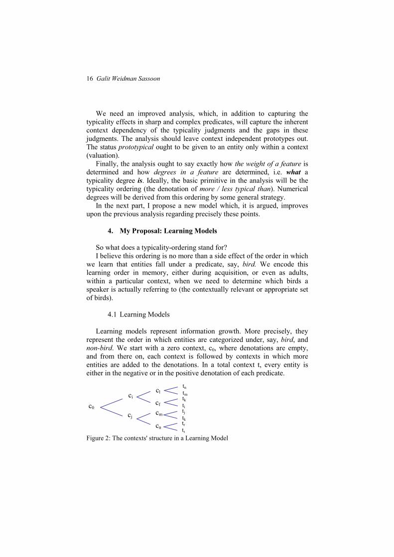
4.1 Learning Models
Learning models represent information growth. More precisely, they
represent the order in which entities are categorized under, say, bird, and
non-bird. We start with a zero context, c0, where denotations are empty,
and from there on, each context is followed by contexts in which more
entities are added to the denotations. In a total context t, every entity is
either in the negative or in the positive denotation of each predicate.
Figure 2: The contexts' structure in a Learning Model
cl
M c0
ci
cm
cn
tn tm
tj tk
tk ti
tr ts
cf
cj
Typicality: An Improved Semantic Analysis 17
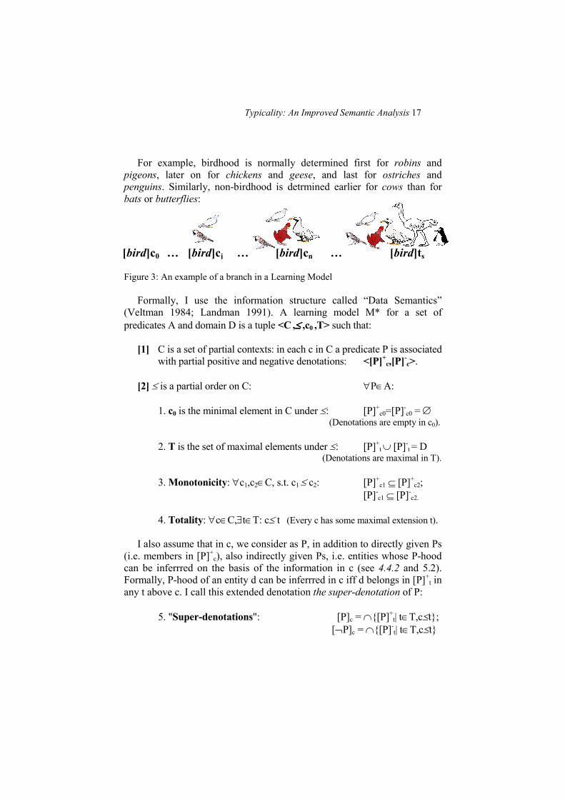
For example, birdhood is normally determined first for robins and
pigeons, later on for chickens and geese, and last for ostriches and
penguins. Similarly, non-birdhood is detrmined earlier for cows than for
bats or butterflies:
Figure 3: An example of a branch in a Learning Model
Formally, I use the information structure called “Data Semantics”
(Veltman 1984; Landman 1991). A learning model M* for a set of
predicates A and domain D is a tuple <C ,≤≤≤≤ ,c0 ,T> such that:
[1] C is a set of partial contexts: in each c in C a predicate P is associated
with partial positive and negative denotations: <[P]+c,[P]
-c>.
[2] ≤ is a partial order on C: ∀P∈A:
1. c0 is the minimal element in C under ≤: [P]+c0=[P]
-c0 = ∅
(Denotations are empty in c0).
2. T is the set of maximal elements under ≤: [P]+t ∪ [P]
-t = D
(Denotations are maximal in T).
3. Monotonicity: ∀c1,c2∈C, s.t. c1 ≤ c2: [P]+c1 ⊆ [P]
+c2;
[P]-c1 ⊆ [P]
-c2.
4. Totality: ∀c∈C,∃t∈T: c≤ t (Every c has some maximal extension t).
I also assume that in c, we consider as P, in addition to directly given Ps
(i.e. members in [P]+c), also indirectly given Ps, i.e. entities whose P-hood
can be inferrred on the basis of the information in c (see 4.4.2 and 5.2).
Formally, P-hood of an entity d can be inferrred in c iff d belongs in [P]+t in
any t above c. I call this extended denotation the super-denotation of P:
5. "Super-denotations": [P]c = ∩{[P]+t| t∈T,c≤t};
[¬P]c = ∩{[P]-t| t∈T,c≤t}
[bird]c0 … [bird]cj … [bird]cn … [bird]ts
18 Galit Weidman Sassoon
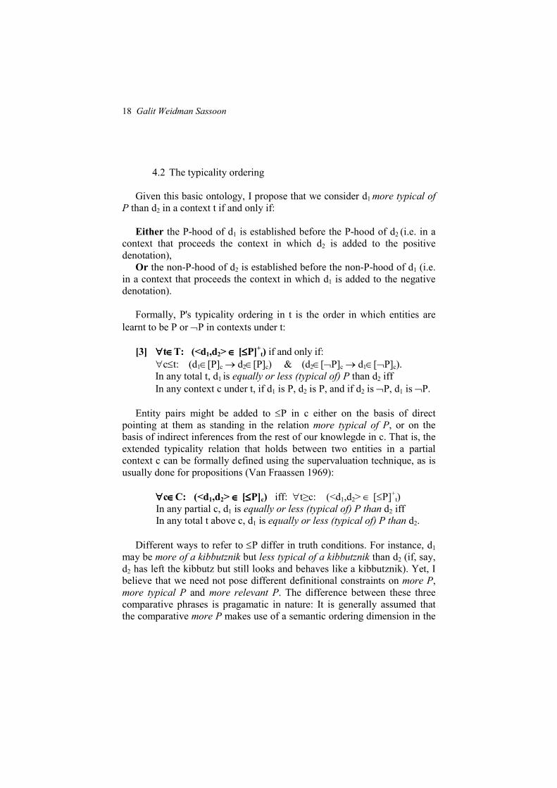
4.2 The typicality ordering
Given this basic ontology, I propose that we consider d1 more typical of
P than d2 in a context t if and only if:
Either the P-hood of d1 is established before the P-hood of d2 (i.e. in a
context that proceeds the context in which d2 is added to the positive
denotation), Or the non-P-hood of d2 is established before the non-P-hood of d1 (i.e.
in a context that proceeds the context in which d1 is added to the negative
denotation).
Formally, P's typicality ordering in t is the order in which entities are
learnt to be P or ¬P in contexts under t:
[3] ∀∀∀∀t∈∈∈∈T: (<d1,d2> ∈∈∈∈ [≤≤≤≤P]+t) if and only if:
∀c≤t: (d1∈[P]c → d2∈[P]c) & (d2∈[¬P]c → d1∈[¬P]c).
In any total t, d1 is equally or less (typical of) P than d2 iff
In any context c under t, if d1 is P, d2 is P, and if d2 is ¬P, d1 is ¬P.
Entity pairs might be added to ≤P in c either on the basis of direct
pointing at them as standing in the relation more typical of P, or on the
basis of indirect inferences from the rest of our knowlegde in c. That is, the
extended typicality relation that holds between two entities in a partial
context c can be formally defined using the supervaluation technique, as is
usually done for propositions (Van Fraassen 1969):
∀∀∀∀c∈∈∈∈C: (<d1,d2> ∈∈∈∈ [≤≤≤≤P]c) iff: ∀t≥c: (<d1,d2> ∈ [≤P]+t)
In any partial c, d1 is equally or less (typical of) P than d2 iff
In any total t above c, d1 is equally or less (typical of) P than d2.
Different ways to refer to ≤P differ in truth conditions. For instance, d1
may be more of a kibbutznik but less typical of a kibbutznik than d2 (if, say,
d2 has left the kibbutz but still looks and behaves like a kibbutznik). Yet, I
believe that we need not pose different definitional constraints on more P,
more typical P and more relevant P. The difference between these three
comparative phrases is pragamatic in nature: It is generally assumed that
the comparative more P makes use of a semantic ordering dimension in the
Typicality: An Improved Semantic Analysis 19
meaning of P (Kamp 1995; Bartch 1984, 1986). Conversely, more typical
(of a) P makes use of different, or additional, ordering properties, namely,
criteria from world knowledge, not just semantic criteria. Finally, relevant
P makes use of completely ad-hoc properties, not just world knowledge or
semantic criteria. The effect of the ordering criteria on the ordering relation
(and of the ordering relation on the ordering criteria) will be further
discussed in 4.9-4.10. At this point, note only that, as desired, a possibly
different ordering relation may be associated with a predicate in each
context. This much context dependency is required in order to capture the
typicality effects correctly (for further discussion of this point, see 4.8).
In the rest of part 4 we will see that a number of long-standing puzzles
are now solved.
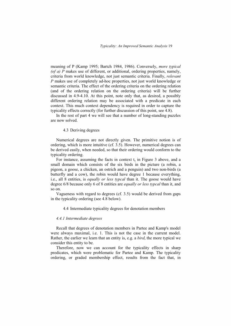
4.3 Deriving degrees
Numerical degrees are not directly given. The primitive notion is of
ordering, which is more intuitive (cf. 3.5). However, numerical degrees can
be derived easily, when needed, so that their ordering would conform to the
typicality ordering.
For instance, assuming the facts in context ts in Figure 3 above, and a
small domain which consists of the six birds in the picture (a robin, a
pigeon, a goose, a chicken, an ostrich and a penguin) and two non-birds (a
butterfly and a cow), the robin would have degree 1 because everything,
i.e., all 8 entities, is equally or less typcal than it. The goose would have
degree 6/8 because only 6 of 8 entities are equally or less typcal than it, and
so on.
Vagueness with regard to degrees (cf. 3.5) would be derived from gaps
in the typicality ordering (see 4.8 below).
4.4 Intermediate typicality degrees for denotation members
4.4.1 Intermediate degrees
Recall that degrees of denotation members in Partee and Kamp's model
were always maximal, i.e. 1. This is not the case in the current model.
Rather, the earlier we learn that an entity is, e.g. a bird, the more typical we
consider this entity to be.
Therefore, now we can account for the typicality effects in sharp
predicates, which were problematic for Partee and Kamp. The typicality
ordering, or graded membership effect, results from the fact that, in
20 Galit Weidman Sassoon
acquisition, or while disambiguating predicate meaning within a particular
context, speakers encode different bird types in memory gradually.
(Consider for a moment the predicate prime number. Despite its clear
formal definition, the status of very big numbers with respect to prime is
yet to be discovered by mathematicians!)
In Partee and Kamp 1995, the denotations of non-vague predicates (e.g.
bird) are represented as total, Fregean entities, independent of speakers'
experience or belief. But we already saw that typicality is connected to the
set of entities which a speaker knows and considers relevant in a context
(cf. 1; 3.4; 4.2). Moreover, the graded structure proposed in 4.2 does not
interfere with the assumption that the denotation of bird, unlike the
denotation of chair, though learnt gradually, is (normally) already fully
specified in actual contexts of utterance. It is quite plausible to assume that
it is already fully specified earlier in the context structure than the
denotation of chair (which is more inherently vague). That is, the
difference between vague and non-vague predicates (+/- Vague) is of
quantity, more than of quality.
Finally, this intuitively felt difference between vague and non-vague
predicates may have to do with other factors besides the level of vagueness
in the denotation. Clearly, no speaker carries in mind an infinite list of all
birds and non-birds. Crucially, an algorithm that enables speakers to
determine the birdhood, or non-birdhood, of every new entity, can replace
the assumption that the bird denotations are fully specified.
In 5.2 we discuss one such algorithm. We will see that the specification
of only a few birds and a set of features allows speakers to automatically
determine the birdhood of new items. The status of a novel item remains
undetermined only if every known bird scores better than that item in the
bird features, and that item scores better than every known non-bird in the
bird features. However, this algorithm also applies to vague predicates like
chair. Therefore, I would now like to draw attention to another algorithm,
which, crucially, affects vague and non-vague predicates differently.
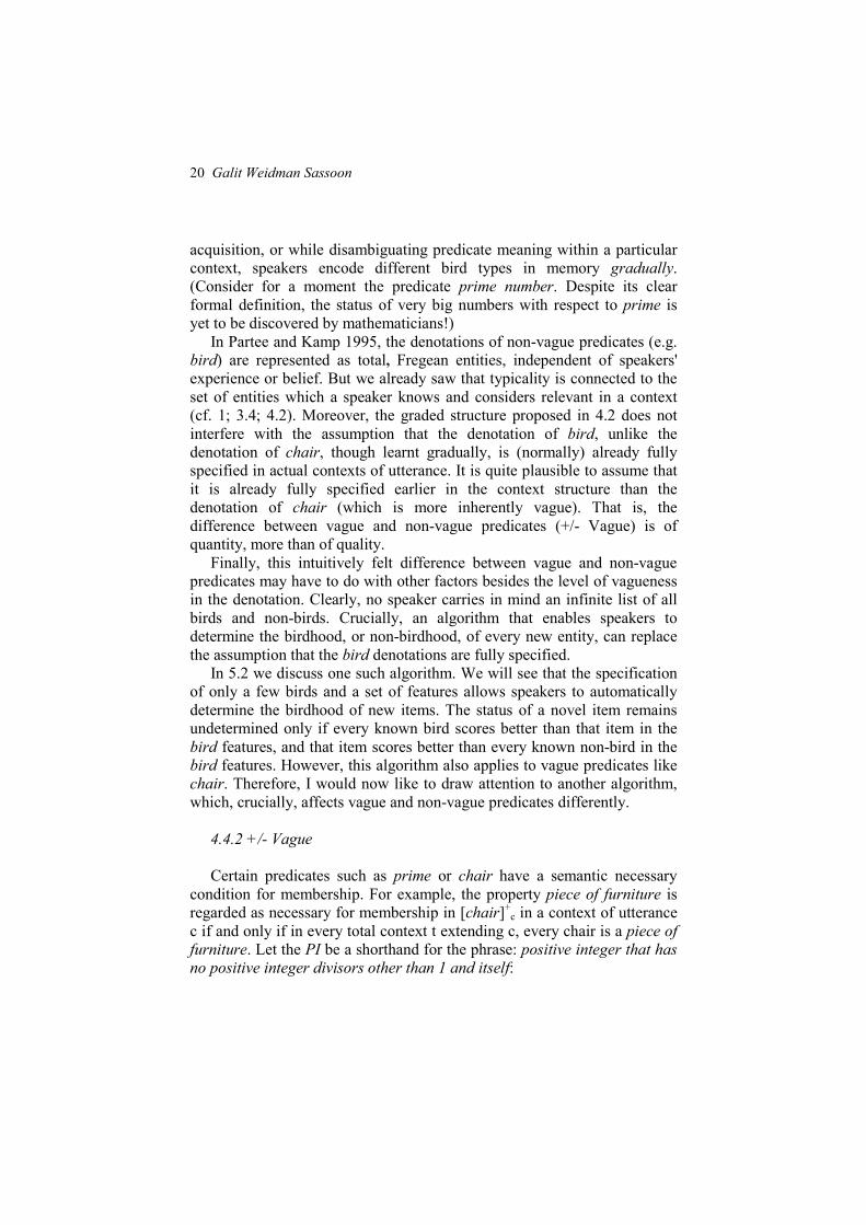
4.4.2 +/- Vague
Certain predicates such as prime or chair have a semantic necessary
condition for membership. For example, the property piece of furniture is
regarded as necessary for membership in [chair]+c in a context of utterance
c if and only if in every total context t extending c, every chair is a piece of
furniture. Let the PI be a shorthand for the phrase: positive integer that has
no positive integer divisors other than 1 and itself:
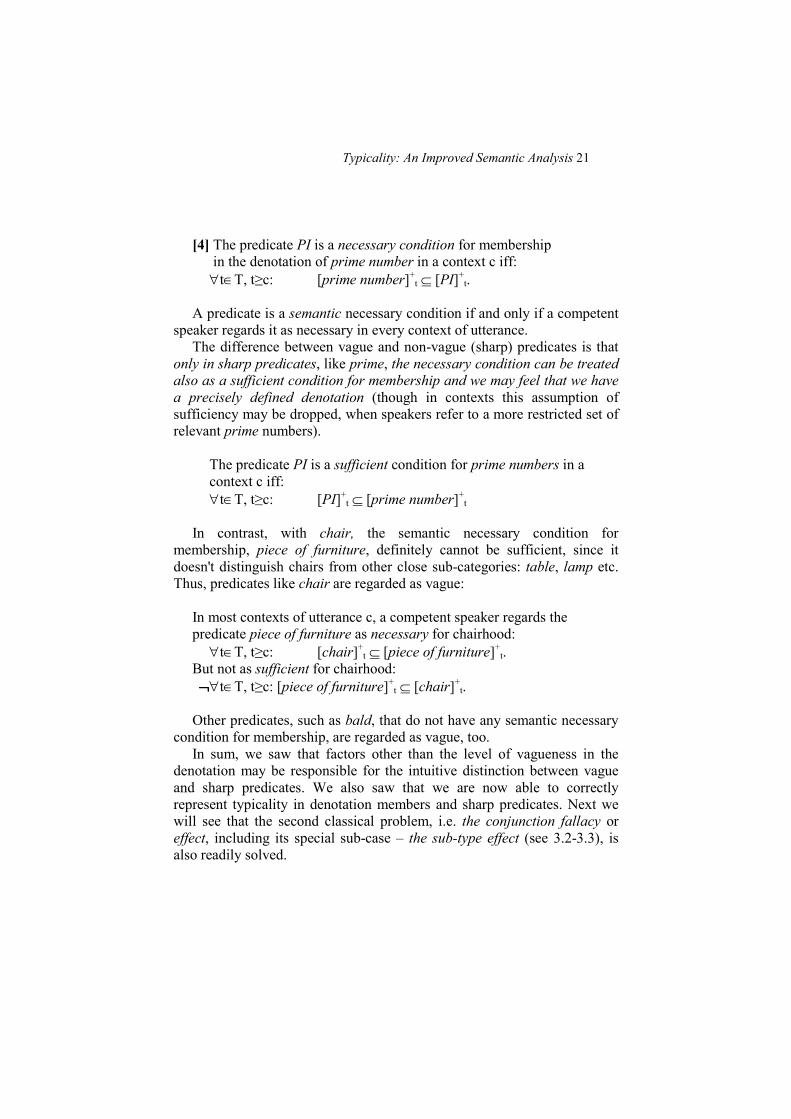
Typicality: An Improved Semantic Analysis 21
[4] The predicate PI is a necessary condition for membership
in the denotation of prime number in a context c iff:
∀t∈T, t≥c: [prime number]+t ⊆ [PI]
+t.
A predicate is a semantic necessary condition if and only if a competent
speaker regards it as necessary in every context of utterance.
The difference between vague and non-vague (sharp) predicates is that
only in sharp predicates, like prime, the necessary condition can be treated
also as a sufficient condition for membership and we may feel that we have
a precisely defined denotation (though in contexts this assumption of
sufficiency may be dropped, when speakers refer to a more restricted set of
relevant prime numbers).
The predicate PI is a sufficient condition for prime numbers in a
context c iff:
∀t∈T, t≥c: [PI]+t ⊆ [prime number]
+t
In contrast, with chair, the semantic necessary condition for
membership, piece of furniture, definitely cannot be sufficient, since it
doesn't distinguish chairs from other close sub-categories: table, lamp etc.
Thus, predicates like chair are regarded as vague:
In most contexts of utterance c, a competent speaker regards the
predicate piece of furniture as necessary for chairhood:
∀t∈T, t≥c: [chair]+t ⊆ [piece of furniture]
+t.
But not as sufficient for chairhood:
¬¬¬¬∀t∈T, t≥c: [piece of furniture]+t ⊆ [chair]
+t.
Other predicates, such as bald, that do not have any semantic necessary
condition for membership, are regarded as vague, too.
In sum, we saw that factors other than the level of vagueness in the
denotation may be responsible for the intuitive distinction between vague
and sharp predicates. We also saw that we are now able to correctly
represent typicality in denotation members and sharp predicates. Next we
will see that the second classical problem, i.e. the conjunction fallacy or
effect, including its special sub-case – the sub-type effect (see 3.2-3.3), is
also readily solved.
22 Galit Weidman Sassoon
4.5 The sub-type effect
Sub-type effects can now be accounted for: The typicality degree of
ostriches is greater in the predicate ostrich than in bird: if they are
categorized late in bird, relative to other bird types, but early in ostrich,
relative to other ostriches! Since this is a natural state of affairs, in most
contexts typical ostriches are indeed considered as atypical birds.
For example, in the birds' model given in 4.3 above, the ostrich has a
degree 2/8 in bird, because only 2 of 8 entities are equally or less typical
than it in bird. Hence, it is an atypical bird in ts. Yet, we can reasonably
assume that this entity is the first member in the denotation of ostrich in ts,
i.e. its degree in ostrich is 1. Thus, it is both an atypical bird and a very
typical ostrich in ts.
4.6 The conjunction effect
Conjunction effects or fallacies are similarly accounted for: The degree
of brown apples is greater in brown-apples than in apple, when they are
categorized late under apple, relative to other apple-types (red, green etc.),
but early under brown apple, relative to other brown apples.
Similarly, the typical male-nurses are atypical males when the earliest
known males are not nurses. The typical male-nurses are also atypical
nurses when the earliest known nurses are not males.
These facts fall into place without any new stipulations for complex
predicates.
4.7 The negation effect
Negation effects are also accounted for without any new stipulations.
The ordering of non-bird is, by the definition of a typicality ordering in 4.2,
inverse to the ordering of bird in each context (for supporting evidence, see
Smith et al 1988).
Exceptions to this generalization (cf. 2.1) are accounted for, since this
inverse pattern is predicated only for the logical negation of a predicate. If a
negated predicate like non-bird is contextually restriced to, say – animals,
then it is not equivalent to the logical negation of bird and hence its
ordering is not predicted to be inverse to the ordering of bird.
Typicality: An Improved Semantic Analysis 23
The third classical problem is the representation of partial and context
dependent knowledge about typicality (see 3.4, 3.6). Let us see how the
current proposal handles in these issues as well.
4.8 Partial knowledge
In a learning model, typicality degrees or relations may be unknown: A
pair, say – a penguin and an ostrich, is in the gap of the ordering more
typical of a bird in a context c, if it is still possible in c (i.e. true in some
context following c) that the penguin is more typical in bird, and it is still
possible that the ostrich is more typical in bird.
For example, if in context cl in the learning model in Figure 2 (see 4.1),
the penguin is already known to be a bird, but the ostrich is not yet known
to be a bird, and in context cf the ostrich is already known to be a bird but
the penguin is not yet known to be a bird, then, in context ci we do not yet
know which bird is more typical, the penguin or the ostrich.
4.9 Context dependency
4.9.1 Context dependent ordering relations
The inherent context dependency of the typicality judgments is now
predicted. Context independent (or valuation-independent) ordering
relations are not part of the theory. As desired, the typicality ordering is
defined per total context in the learning model.
But how is a contextual typicality ordering fixed? Context dependency
in the interpretation of domains of quantifiers and conditionals is accounted
for (Kadmon and Landman 1993; von Fintel 1994) by assuming that a set
of properties restricts the domain to the set of relevant members in each
context. Similarly, it is plausible that, within context, a set of properties
(features) restricts predicate denotations to the set of relevant denotation
members, those members, which the speaker is actually referring to (for a
detailed discussion of the mechanism in which denotations are contextually
restricted via properties, see Kadmon and Landman 1993; Sassoon 2002;
and also 4.10 below).
Given this set of restricting features, the relevant typicality ordering of a
predicate P in each context of utterance, is the ordering of the conjunction
of P and its restricting properties. For example, chickens usually precede
robins in being regarded as both birds and walking in the barnyard. Hence,
their typicality degree in bird in the context of the utterance birds walking
24 Galit Weidman Sassoon
in the barnyard is predicted to exceed that of robins, as Roth and Shoben
indeed found (see part 1).
4.9.2 Context dependent prototypes
Context independent (or valuation-independent) prototypes, in
particular, are not part of the theory at all (cf. 2.3.1, stipulation [5] in Partee
and Kamp's model). In the current proposal, in each context, some entities
are the best in each predicate: The earliest entities, among the available
entities, which are known to be denotation members. In this way, we
account for the ordering in typical tall person despite the fact that, out of
context, there is no maximal tallness.
In addition, eliminating the prototypes from the theory considerably
simplifies the taxonomy of predicates: The distinction between predicates
without a prototype, predicates with a prototype that does not affect the
denotation, and predicates with a prototype that affects the denotation (cf.
2.3.1, stipulation [6]), is eliminated.
The intuitively felt differences between these predicate types is
accounted for, again, in a quantitative rather than qualitative manner. These
differences are induced by different extents of context dependency in the
meaning of the predicate and its derived comparative. For example, in
taller, the ordering criterion, and hence the ordering relation, is fixed
semantically. But in more typical of a tall person, player, tree etc., typical
associates more features with the predicate tall (context dependent ordering
criteria). So the NP typical tall person, like typical bird, associates with a
context dependent ordering relation. Such a context dependent ordering
relation must be indicated by the operator typical.
4.9.3 +/–Gradable, +/–Prototype
Put more formally, +Gradable predicates, like tall and bald, (i.e.
predicates that can directly combine with more) are distinguished from –
Gradable predicates, like bird (that cannot combine with more unless
modified by an operator like typical), in the following way:
Predicates like bald may not have a necessary condition for membership
(cf. 4.4), but they do have a semantic ordering feature (see 4.10 for the
definition of such a feature). Moreover, crucially, this ordering feature can
be treated as a necessary condition for membership in the derived
comparative ≤bald in a context of utterance c:
Typicality: An Improved Semantic Analysis 25
∀t∈T, t≥c: [is more bald]+t ⊆ [has less hair]
+t
i.e. if d1 is more bald than d2, then d1 has less hair than d2.
This single ordering feature can be treated also as sufficient for
membership in the ordering relation in c, and hence, we may feel that we
have a precisely defined ordering relation:
∀t∈T, t≥c: [has less hair]+t ⊆ [is more bald]
+t
Other predicates, like bird or prime, do not have a single ordering
feature: Out of context they have no semantic ordering criterion at all, and
within contexts they are frequently associated with several ordering criteria
(Kamp 1975). This can even happen with gradable adjectives like bald
when, say – psychological features related to baldness are treated as
ordering bald by typicality. In these contexts, has less hair cannot be
treated as sufficient for membership in the ordering relation ≤bald, because
one may be grasped as balder (or as more typical of a bald person) than
other people with an equal or greater amount of hair (which nonetheless
are psychologically more influenced by their baldness). When nothing is
treated as necessary and sufficient for membership in the ordering relation,
it remains vague and the predicate is felt to be –Gradable.
However, when a –Gradable predicate is associated with a set of
ordering features, we do have partial knowledge regarding the ordering of
entities. In particular, best cases can be identified: Those entities that satisfy
all the ordering features are regarded as prototypes. Hence, predicates like
chair, bird or flu are normally regarded as + Prototype.
This proposal predicts that a complex predicate would not be grasped as
gradable even if its parts are gradable. In fact, such predicates do not
combine with more:
7) * d1 is more midget giant than d2
8) * d1 is more fat bald than d2
9) * d1 is more clean tall than d2
They have two potential ordering criteria, so neither functions as
sufficient for membership in their ordering relation. The appropriateness of
more P seems to depend on the existence of a sufficient ordering criterion.
In fact, even when P is sharp, more P improves whenever such a criterion
becomes salient (e.g. more pregnant).
26 Galit Weidman Sassoon
What about multi-dimensional gradable predicates such as healthy?
These predicates seem to be misrepresented in the current proposal. They
are felt to be +Gradable, not +Prototype (they directly combine with more),
despite the fact that they are associated with a set of dimensions, not a
single ordering dimension! For instance, one may be regarded as healthy if
one is generally healthy, i.e. healthy with respect to hair, heart, blood
pressure, fever, skin etc. None of the comparatives derived from these
dimensions (nor the conjunction healthier with respect to hair and
healthier with respect to heart and…) can be treated as necessary and
sufficient for membership in the comparative ≤healthy (for example, one
may be regarded generally healthier than others, while being less healthy
with respect to, say, the skin). Yet, healthy can directly combine with more.
I believe that multi-dimensional gradable predicates like healthy are not
associated with a set of ordering features in precisely the same way that
+Prototype predicates, such as bird, are. In multi-dimensional gradable
predicates we use (even explicitly), quantification over ordering
dimensions, or respects (Bartch 1984; 1986): generally healthy, healthy in
every respect etc. (i.e., a universal or generic quantifier ranges over the
variety of ordering dimensions). The predicate is ordered by one dimension
at a time. This is not the case with +Prototype –Gradable predicates like
bird. Indeed, we do not usually say, or intend to say, that an entity is
generally a bird or a bird in every respect.
4.10 Typicality features
Finally, the fourth classical problem, i.e. that of defining the notion of a
typicality feature (or an ordering dimension), can now be dealt with. For
each predicate P, speakers consider certain features as typical of P, e.g
feathers, small, flies and sings are normally regarded as typical of birds. In
addition, it is common in Philosophy and Psychology to assume that each
feature is assigned a weight, and generally, the typicality degree of say, a
robin in bird, is indicated by the weighted-mean of its degrees in all the
bird features: How well it scores in flies, sings, small etc. However,
scholars still cannot tell the exact conditions under which a property is
regarded as a typicality feature and they hardly agree about how a weight
of a feature is determined.
Typicality: An Improved Semantic Analysis 27
4.10.1 Ceteris paribus correlation
Having stated what a typicality ordering is (cf. 4.2), we can now state that
a property like flying or being-small counts as a typicality feature of a
predicate like bird iff the ordering in the feature correlates with the ordering
in bird ceteris paribus i.e.:
[5] Any entity more typical in flying than other entities, and not less
typical in other features like small, is more typical of a bird.
Exceptions (items which are more typical in flying but less typical in
bird or vice versa) are allowed when (and only when) the ordering in two
bird-features (e.g. flying and small) is inverse.
4.10.2 Feature weights
Given this generalization, we can now state that the greater the overlap
between the typicality ordering (the set of entity pairs where the former
entity is more typical than the latter entity) of a feature and the typicality
ordering of bird, the higher the feature’s weight, i.e. the more central it is
considered in ordering birds. Formally, the weight of a typicality feature F
is indicated by the extent of overlap between (or the relative size of the
intersection of) its orderings, ≤F, and P’s ordering, ≤P:
[6] The weight of F in P : = |([≤F]t ∩[≤P]t)|/|(D×D)|
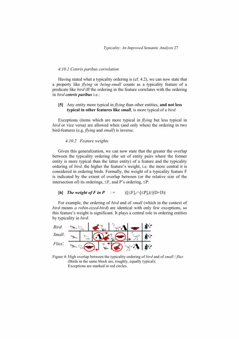
For example, the ordering of bird and of small (which in the context of
bird means a robin-sized-bird) are identical with only few exceptions, so
this feature’s weight is significant. It plays a central role in ordering entities
by typicality in bird:
Figure 4: High overlap between the typicality-ordering of bird and of small / flies
(Birds in the same block are, roughly, equally typical);
Exceptions are marked in red circles.
Bird:
Small:
Flies:
28 Galit Weidman Sassoon
However, a property might exist, like – animal, with an ordering which
correlates ceteris paribus with the ordering in bird as required, i.e. any
entity more typical in animal than other entities, and not less typical in
other bird features, is more typical of a bird. However, the overlap between
the ordering of bird and that of animal is poor, since many typical animals
are atypical birds (most of them are actually not birds at all). Therefore, the
feature weight of animal is not significant.
We can now assume that the set of predicates in our language also
consists of (in addition to 'normal' predicates, which denote sets of
individuals) predicates of the form: a typical feature of P. These predicates
denote sets of features. The denotations of these predicates grow gradually
through contexts, just like any other predicate denotation (for a detailed
discussion of a model with such feature sets, see Sassoon 2002).
5. What exactly do Learning Models model? More findings
In part 4, we saw that, by assuming that the typicality ordering is no
more than a partial order, which stands for the order in which entities are
learnt to be members or non-members in a denotation, we shed light on a
variety of typicality effects which are traditionally regarded as puzzling.
However, two more clarifications with regard to the concept “learning
order” are required. Both have to do with the fact that the learning order as
it is encoded in memory is not always equivalent to the actual temporal
order in which items are added to the denotation, due to two factors.
5.1 Corrections
The first factor has to do with our ability to make corrections in our
knowledge. What if my initial exposure to birds was through ostriches??
Initially, I would think that ostriches are representative birds. Later on, I
would have to correct my beliefs. Formally, I would jump to a different
branch in the context-structure, where ostriches are indeed represented as
less typical than other birds. Indeed, it is known that first exposure to an
atypical item slows down acquisition (Mervis & Pani 1980). Why? Because
learners induce wrong category features: For instance, in our example,
wrong optimal size, running instead of flying etc.
Typicality: An Improved Semantic Analysis 29
5.2 Inferences: Indirect learning
The second factor has to do with indirect learning, i.e. with our ability to
add items to the denotation even if they were never given to us as such. We
can infer the membership of certain new items by using the knowledge
given to us already by the known denotation members and features. I
assume that – if one has knowledge about the bird features (unlike the
children in the experiments of Mervis & Pani 1980, just cited) – then new,
previously unavailable entities, which are better than known birds in the
bird-features, once they become available, are automatically regarded as
birds, too (otherwise rule [5] in 4.10.1 will be violated; Sassoon 2002). So
we have a learning algorithm which overcomes arbitrary gaps in our
learning order. For example, categorization of, say – a chicken or a goose,
in bird – implies the bird-hood of anything more typical than a chicken or a
goose, like a duck, once it is available. Indeed, it is also known that
previously unavailable typical instances are frequently (falsely) assumed to
be known: (Reed 1988). Why? Given their high scores in the typicality
features, they should already be known denotation members!
But, not so for atypical ones. For example, if the known birds are
robins, pigeons, geese and chickens, in the exposure to ostriches we would
not infer their bird-hood automatically. They would remain in the gap
because it is still possible that they diverge too much from the known birds.
Hence, they are regarded as less typical.
An intruiguing evidence for indirect learning of this sort was found in a
study of aphasic patients by Kiran & Thompson, which was based on
previous findings in neural network simulations. These studies demonstrate
that exposure to a whole range of atypical items and features results in
spontaneous recovery of categorization of untrained more typical items, but
not vice versa.. That is, the membership of more typical instances can be
indirectly automatically inferred from the membership of less typical
instances, but not vice versa, as predicted.
5.3 Conclusions of part 5
Initially, direct learning of the category membership of certain entities
occurs, and possibly also direct learning of certain typicality features. The
order of learning the category members is encoded in memory. Then, this
ordering is enriched and corrected, based on indirect inferences. If the
learning-order of a property highly correlates with the category learning-
order, this property is treated as a typicality feature, too. In addition, in the
30 Galit Weidman Sassoon
exposure to new entities, more entities are added to the denotation. If the
new entities score highly in the typicality features, corrections in the
learning order are made, such that these entities are encoded as typical. In
this way, speakers overcome the effects of arbitrary gaps in their learning
order.
6. Conclusions
In addition to the coupling between typicality and learning (which is
demonstrated by a range of studies), learning models capture a wide range
of typicality effects which were long-standing puzzles. These puzzles
include the typicality effects in sharp and complex predicates (in particular
the conjunction effect /fallacy), the context dependency and partiality of the
knowledge about the typicality relations and degrees, and the definition of a
feature and a feature weight.
Unlike previous theories (fuzzy models or supermodels), the current
proposal predicts the typicality effects in complex predicates without any
new stipulations for the purpose, i.e. without a complement rule for negated
predicates and a minimal degree rule (cf. 2.1) or a modified membership
function (cf. 2.3.2) for modified nouns.
By insisting on a highly context dependent representation for the
typicality ordering, a number of theoretical entities are eliminated from the
analysis, among which are the context independent prototypes and the
measure functions.
The coupling between typicality and membership is captured via the
gradual learning of the denotation members. This spares us the need to
stipulate two separate sets of values for the membership function and the
typicality function, and renders the theory more elegant.
In addition, the taxonomy of predicate types is drastically simplified.
The intuitively felt differences between predicate types are accounted for
using the (well-defined) notions of ordering features, of necessary and
sufficent conditions for membership, and of partial ordering relations.
Unlike the measure function over sets of valuations, these notions are
psychologically real: There is abundant evidence that speakers associate
predicates with partial sets of ordering relations, ordering features, and
necessary conditions for membership.
Given the elegance and the wide array of predictions of the learning
model, it seems that our understanding of the typicality effects and their
relation to predicate meaning, has considerably improved.
Typicality: An Improved Semantic Analysis 31
References
Aarts, Bas, David Denison, Evelien Keizer, and Gergana Popova (eds.)
2004 Fuzzy Grammar, a Reader. Oxford University Press.
Armstrong, Lee, Lila Gleitman, and Henry Gleitman
1983 What some concepts might not be. Cognition 13: 263-308.
Bartsch, Renate,
1986 Context dependent interpretations of lexical items, J. Groenendijk,
D. de Jongh, M. Stokhof (eds.) Foundations of Pragmatics and
Lexical semantics, GRASS 7, Foris, Dordrecht.
1984 The structure of word meanings: Polysemy, Metaphor, Metonymy.
In: Landman Fred & Veltman Frank (Eds.), Varieties of Formal
semantics, GRASS 3, Foris, Dordrecht.
Barsalou, Lawrence
1983 Ad hoc categories. Memory and Cognition 11: 211-227.
Batting W.F. and Montague W.E.,
1969 Category Norms for Verbal Items in 56 Categories. Journal of
Experimental Psychology Monograph 80 (3) Pt. 2.
Brooks, L.R.
1987 Nonanalytic cognition In U. Neisser (Eds.), Concepts and
Conceptual Development: Ecological and intellectual factors in
categorization, 141-74, Cambridge University Press.
Costello, Fintan 2000 An exemplar model of classification in simple and combined
categories. In: Proceedings of the Twenty-Second Annual
Conference of the Cognitive Science society, Lila.Gleitman and
K. Joshi (eds.), 95-100. Mahwah, N. J.: Erlbaum.
Dayal, Veneeta,
2004 Number Marking and (In)definiteness in Kind Terms. Linguistics
and Philosophy 27(4): 393 – 450.
Fein, Kieth,
1975 Truth, Vagueness and Logics, Synthese 30: 265-300.
Gardenfors, Peter
2004 Conceptual Spaces, The Geometry of Thought. MIT Press.
Hampton, James
1997 Conceptual Combination. In: Knowledge, Concepts and
Categories, Koen Lamberts and David Shanks (eds.), 135-162. Cambridge,
MA: The MIT Press.
Heit, Evan
1997 Knowledge and concept learning. In: Knowledge, Concepts and
Categories, Koen Lamberts and David Shanks (eds.), 135-162.
Cambridge, MA: The MIT Press.
Kadmon, Nirit, and Fred Landman,
1993 Any. Linguistics And Philosophy 16: 353-422.
32 Galit Weidman Sassoon
Kamp, Hans
1975 Two theories about Adjectives. In: Edward Keenan (ed.), Formal
Semanticvs for Natural Language.
Keil, Frank
1987 Conceptual development and category structure. In: Concepts
And Conceptual Development, Ulrich Neisser (ed). Cambridge
University Press.
Kiran, Swathi and Cynthia Thompson,
2003 The role of semantic complexity in treatment of naming deficits:
Training categories in fluent aphasia by controlling exemplar
typicality. Journal of Speech Language and Hearing Research
46: 608-622.
Klein, Ewan.
1980 A semantics for positive and comparative adjectives. Linguistics
and Philosophy 4:1–45.
Lakoff, George
1973 Hedges: a study in meaning criteria and the logic of fuzzy
concepts. Journal of Philosophical logic 2: 458-508.
1987 Women, Fire and Dangerous Things: What Categories Reveal
about the Mind. Chicago University Press.
Landau, Barbara
1982 Will the real grandmother please stand up? The psychological
reality of dual meaning representations. Journal of
Psycholinguistic Research 11(1): 47-62.
Landman, Fred
1991 Structures For Semantics. Dordrecht: Kluwer Academic
Publishers.
Lynott, Dermot, and Michael Ramscar
2001 Can we model conceptual Combination using distributional
Information, 12th Irish Conference on Artificial Intelligence and
Cognitive Science 5.9-7.9.
Mervis, Carolyn, and Eleanor Rosch
1981 Categorization of natural objects. Annual review of psychology
32: 89-115.
Mervis, Carolyn, and John Pani
1980 Acquisition of basic object categories. Cognitive Psychology 12:
496-522.
Murphy, Gregory, and Douglas Medin
1985 The role of theories in conceptual coherence. Psychological
Review 92(3): 289-316.
Typicality: An Improved Semantic Analysis 33
Murphy, Gregory, and Mary Lassaline
1997 Hierarchical structure in concepts and the basic level of
categorization. In: Knowledge, Concepts and Categories, Koen
Lamberts and David Shjanks (eds.), 93-131.Cambridge, MA: The
MIT press.
Murphy and Smith
1982 Basic level superiority in picture categorization. Jurnal of Verbal
Learning and Verbal Behaviour 21: 1-20.
Osherson, Daniel, and Edward Smith
1981 On the adequacy of prototype theory as a theory of concepts.
Cognition 11: 237-262.
Osherson, D.N. And E.E. Smith, O.Wilkkie, A.Lopez, E.Shafir,
1990 Category Based Induction" Psychological Review 97: 185-200.
Partee, Barbara, and Hans Kamp
1995 Prototype theory and compositionality. Cognition 57: 129-91.
Reed, Stephen
1988 Cognition, Theory and Applications. Pacific Grove: Brooks/Cole.
Rips, Lance
1975 Inductive judgments about natural categories. Jurnal of Verbal
Learning and Verbal Behaviour 14: 665-81.
Rosch, Eleanor
1973 On the internal structure of perceptual and semantic categories. In:
Cognitive Development and the Acquisition of Language, T. E.
Moore (ed.), New York: Academic Press.
Roth Emilie and Edward Shoben
1983 The effect of context on the structure of categories. Cognitive
Psychology 15: 346-378.
Smith, Edward, Daniel Osherson, Lance Rips, Margaret Keane
1988 Combining prototypes, a selective modification model. Cognitive
Science 12: 485-527.
Sassoon, Galit
2002 Semantics with clusters of properties. In: Proceedings Of Israel
Association For Theoretical Linguistics 18, Yehuda Falk (ed.), Bar
Ilan University.
2004 Review of: Aarts, Bas; Denison, David; Keizer, Evelien; Popova,
Gergana (2004) Fuzzy Grammar, a Reader, Oxford University
Press. The linguist list: http://linguistlist.org/issues/15/15-
3335.html.
2005 The notion of typicality. In: Proceedings of From Gram to Mind,
Mai 19-21, Bordeaux (www.post.tau.ac.il/~gala).
Shanks, David, and M.F St. John
1994 Characteristics of dissociable human learning systems.
Behavioral and Brain Sciences 17(3): 367-447.
34 Galit Weidman Sassoon
Tversky, Amos, and Danniel Kahneman
1983 Extensional versus intuitive reasoning: the conjunction fallacy in
probability judgments. Psychological Review 90: 293-315.
van Fraassen, B.C.,
1969 Presuppositions, Supervaluations and Free Logic. In: K. Lambert
(Ed.), The Logical Way of Doing Things: 67-91. New Haven:
Yale University Press.
Veltman, Frank
1984 Data Semantics. In: Truth, Interpretation and Information
Proceedings Of The 3rd Amsterdam Colloquium, Jeroen
Groenendijk, Theo Janssen and Martin Stokhof (eds.)
von Fintel, Kai,
1994 Restrictions on Quantifier Domains. PhD Dissertation, Amherst:
University of Massachusetts.
Wittgenstein, Ludwig
1968 Reprint: Philosophical Investigations, Translated By G.E.M
Anscombe, 3rd edition, Oxford: Blackwell. Original edition,
1953.
Zadeh, Lofti
1965 Fuzzy sets, Information and control 8: 338-53.