typing techniques for security in mobile agent systems
TRANSCRIPT

Typing Techniques for Security in Mobile
Agent Systems
Fernando Rosa Velardo
May 2004
Director: David de Frutos Escrig

2

Contents
1 Introduction 9
1.1 Formal methods and computation . . . . . . . . . . . . . . . . . . . . . 91.2 Security . . . . . . . . . . . . . . . . . . . . . . . . . . . . . . . . . . . 101.3 Security protocols . . . . . . . . . . . . . . . . . . . . . . . . . . . . . . 111.4 Mobile computation . . . . . . . . . . . . . . . . . . . . . . . . . . . . . 121.5 Mobile agent systems . . . . . . . . . . . . . . . . . . . . . . . . . . . . 131.6 Mobility and security . . . . . . . . . . . . . . . . . . . . . . . . . . . . 14
1.6.1 Host protection . . . . . . . . . . . . . . . . . . . . . . . . . . . 151.6.2 Agent protection . . . . . . . . . . . . . . . . . . . . . . . . . . 16
1.7 Interpretation of types . . . . . . . . . . . . . . . . . . . . . . . . . . . 191.8 Outline of the work . . . . . . . . . . . . . . . . . . . . . . . . . . . . . 20
2 Nominal Calculi and Cryptographic Primitives 23
2.1 The π-calculus . . . . . . . . . . . . . . . . . . . . . . . . . . . . . . . . 232.2 The Security π-calculus . . . . . . . . . . . . . . . . . . . . . . . . . . . 262.3 The spi-calculus . . . . . . . . . . . . . . . . . . . . . . . . . . . . . . . 282.4 The Distributed π-calculus: Dπ . . . . . . . . . . . . . . . . . . . . . . 34
2.4.1 Syntax and semantics . . . . . . . . . . . . . . . . . . . . . . . . 352.4.2 Errors and types . . . . . . . . . . . . . . . . . . . . . . . . . . 362.4.3 Type system . . . . . . . . . . . . . . . . . . . . . . . . . . . . . 41
3 Ambient Calculus 45
3.1 Syntax and semantics . . . . . . . . . . . . . . . . . . . . . . . . . . . . 453.2 Security in the Ambient Calculus . . . . . . . . . . . . . . . . . . . . . 50
4 Types for the Ambient Calculus 53
4.1 Exchange types . . . . . . . . . . . . . . . . . . . . . . . . . . . . . . . 534.1.1 Communication runtime errors . . . . . . . . . . . . . . . . . . 584.1.2 Multiple arity types . . . . . . . . . . . . . . . . . . . . . . . . . 62
4.2 Types for mobility and opening control . . . . . . . . . . . . . . . . . . 634.2.1 Type syntax and typing rules . . . . . . . . . . . . . . . . . . . 644.2.2 Adding mobility runtime errors . . . . . . . . . . . . . . . . . . 674.2.3 Objective moves . . . . . . . . . . . . . . . . . . . . . . . . . . . 68
3
4 CONTENTS
4.3 Ambient groups . . . . . . . . . . . . . . . . . . . . . . . . . . . . . . . 71
4.3.1 The typed Ambient Calculus with groups . . . . . . . . . . . . . 71
4.3.2 Access control runtime errors . . . . . . . . . . . . . . . . . . . 75
4.3.3 Objective moves . . . . . . . . . . . . . . . . . . . . . . . . . . . 77
4.4 Other type systems . . . . . . . . . . . . . . . . . . . . . . . . . . . . . 78
5 Extensions of the Ambient Calculus 79
5.1 Safe Ambients . . . . . . . . . . . . . . . . . . . . . . . . . . . . . . . . 79
5.1.1 Syntax and semantics . . . . . . . . . . . . . . . . . . . . . . . . 81
5.1.2 Types . . . . . . . . . . . . . . . . . . . . . . . . . . . . . . . . 81
5.1.3 Main results on typed processes . . . . . . . . . . . . . . . . . . 85
5.1.4 Renaming as an example . . . . . . . . . . . . . . . . . . . . . . 85
5.1.5 Authentication, yet another example . . . . . . . . . . . . . . . 86
5.2 Robust Ambients . . . . . . . . . . . . . . . . . . . . . . . . . . . . . . 88
5.3 Controlled Ambients . . . . . . . . . . . . . . . . . . . . . . . . . . . . 89
5.3.1 Syntax and semantics . . . . . . . . . . . . . . . . . . . . . . . . 90
5.3.2 Types . . . . . . . . . . . . . . . . . . . . . . . . . . . . . . . . 91
5.3.3 Main results on typed processes . . . . . . . . . . . . . . . . . . 94
5.3.4 Exclusive simultaneous access: a simple example . . . . . . . . . 94
5.4 Boxed Ambients . . . . . . . . . . . . . . . . . . . . . . . . . . . . . . . 95
5.4.1 Syntax and semantics . . . . . . . . . . . . . . . . . . . . . . . . 95
5.4.2 Types . . . . . . . . . . . . . . . . . . . . . . . . . . . . . . . . 96
5.4.3 Main results on typed processes . . . . . . . . . . . . . . . . . . 98
5.4.4 Example: firewalls revisited . . . . . . . . . . . . . . . . . . . . 99
5.5 NBoxed Ambients . . . . . . . . . . . . . . . . . . . . . . . . . . . . . . 100
5.5.1 Syntax and semantics . . . . . . . . . . . . . . . . . . . . . . . . 100
5.5.2 Types . . . . . . . . . . . . . . . . . . . . . . . . . . . . . . . . 101
5.6 Sealed Boxed Ambients . . . . . . . . . . . . . . . . . . . . . . . . . . . 103
5.6.1 Syntax and Semantics . . . . . . . . . . . . . . . . . . . . . . . 103
5.6.2 Types . . . . . . . . . . . . . . . . . . . . . . . . . . . . . . . . 104
5.6.3 Secrecy theorem . . . . . . . . . . . . . . . . . . . . . . . . . . . 106
5.6.4 Example: Mobile Wide Mouthed Frog Protocol . . . . . . . . . 107
5.7 M3 . . . . . . . . . . . . . . . . . . . . . . . . . . . . . . . . . . . . . . 107
5.7.1 Syntax and semantics . . . . . . . . . . . . . . . . . . . . . . . . 107
5.7.2 Types . . . . . . . . . . . . . . . . . . . . . . . . . . . . . . . . 108
5.7.3 Detecting Trojan horses: a simple example . . . . . . . . . . . . 110
6 Operational Interpretation of Results 113
6.1 Tagged Transitions Systems . . . . . . . . . . . . . . . . . . . . . . . . 113
6.2 Alternative characterization of tagged systems . . . . . . . . . . . . . . 117
6.3 Deriving Tagged Languages . . . . . . . . . . . . . . . . . . . . . . . . 121
6.4 Tagged Dπ . . . . . . . . . . . . . . . . . . . . . . . . . . . . . . . . . 123

CONTENTS 5
7 Conclusions and future work 127
Bibliography 132

6 CONTENTS

List of Figures
2.1 Operational Semantics of the pi-calculus . . . . . . . . . . . . . . . . . 242.2 Wide Mouthed Frog Protocol . . . . . . . . . . . . . . . . . . . . . . . 252.3 Cryptographic version of the Wide Mouthed Frog Protocol . . . . . . . 302.4 Syntax of the Dpi . . . . . . . . . . . . . . . . . . . . . . . . . . . . . . 352.5 Structural equivalence of the Dpi . . . . . . . . . . . . . . . . . . . . . 362.6 Reduction relation of the Dpi . . . . . . . . . . . . . . . . . . . . . . . 362.7 Types and subtyping in the Dpi . . . . . . . . . . . . . . . . . . . . . . 372.8 Runtime errors in the Dpi . . . . . . . . . . . . . . . . . . . . . . . . . 402.9 Typing rules for the Dpi . . . . . . . . . . . . . . . . . . . . . . . . . . 42
3.1 Syntax of the Ambient Calculus . . . . . . . . . . . . . . . . . . . . . . 463.2 Operational Semantics of the Ambient Calculus . . . . . . . . . . . . . 48
4.1 Exchange Types . . . . . . . . . . . . . . . . . . . . . . . . . . . . . . . 544.2 Typing rules for Exchange Types . . . . . . . . . . . . . . . . . . . . . 574.3 Showing an ambient name, a prefix or a message . . . . . . . . . . . . . 594.4 Rules for errors of first class . . . . . . . . . . . . . . . . . . . . . . . . 594.5 Rules for errors of second class . . . . . . . . . . . . . . . . . . . . . . . 604.6 Rules for errors of second class with multiple arities . . . . . . . . . . . 634.7 Mobility Types . . . . . . . . . . . . . . . . . . . . . . . . . . . . . . . 644.8 Rules for errors of the third class . . . . . . . . . . . . . . . . . . . . . 674.9 Types for the Ambient Calculus with groups . . . . . . . . . . . . . . . 734.10 Rules for errors of fourth class . . . . . . . . . . . . . . . . . . . . . . . 764.11 Showing a capability at the top-level . . . . . . . . . . . . . . . . . . . 77
5.1 Ambient Calculus Extensions . . . . . . . . . . . . . . . . . . . . . . . 805.2 ST Types . . . . . . . . . . . . . . . . . . . . . . . . . . . . . . . . . . 825.3 Typing rules for ST types . . . . . . . . . . . . . . . . . . . . . . . . . 845.4 Cab protocol . . . . . . . . . . . . . . . . . . . . . . . . . . . . . . . . 895.5 CA-style cab protocol . . . . . . . . . . . . . . . . . . . . . . . . . . . . 915.6 CA Types . . . . . . . . . . . . . . . . . . . . . . . . . . . . . . . . . . 915.7 Typing rules for CA types . . . . . . . . . . . . . . . . . . . . . . . . . 935.8 Types for MAC Security . . . . . . . . . . . . . . . . . . . . . . . . . . 975.9 MAC errors . . . . . . . . . . . . . . . . . . . . . . . . . . . . . . . . . 98
7

8 LIST OF FIGURES
5.10 NBA Types . . . . . . . . . . . . . . . . . . . . . . . . . . . . . . . . . 1015.11 NBA Typing Rules . . . . . . . . . . . . . . . . . . . . . . . . . . . . . 1025.12 SBA Syntax . . . . . . . . . . . . . . . . . . . . . . . . . . . . . . . . . 1045.13 Reduction and Silent Reduction for SBA . . . . . . . . . . . . . . . . . 1055.14 Types for SBA . . . . . . . . . . . . . . . . . . . . . . . . . . . . . . . 1065.15 M3 Types . . . . . . . . . . . . . . . . . . . . . . . . . . . . . . . . . . 108
6.1 Abstract syntax trees for 1 + (0 × 1) and 1 ⊕ (0� 1) . . . . . . . . . . 1146.2 Commutative diagram induced by a quotient transition system . . . . . 118
7.1 Extended quotient systems lattice . . . . . . . . . . . . . . . . . . . . . 1297.2 The SAC Calculus . . . . . . . . . . . . . . . . . . . . . . . . . . . . . 1307.3 SAC Reduction Relation . . . . . . . . . . . . . . . . . . . . . . . . . . 130

Chapter 1
Introduction
The aim of the present work is to study the existing approaches based on types toprove security properties in systems supporting mobility. The presence of mobilityin the systems introduces many difficulties which have not been fully addressed in asatisfactory way, specially those dealing with security concerns. Static analysis andtype systems in particular can be used within this context for the proof of correctnesswith respect to security properties.
The main goal of this work is to study the state of the art in this field, whiletrying to point out some deficiencies and possible improvements. We will start outby describing the π-calculus and some of its derivates, which form the basis for theformalism we will mostly use, the Ambient Calculus and some of its extensions.
Sometimes we will not present all the details of the formalisms in order to focus onwhat we thought were the most important matters.
1.1 Formal methods and computation
Formal methods offer rigorous techniques for modelling and formally analyzing com-puting systems behaviours. Among them, static program analysis has shown to beone of the most fruitful. Its goal is to check properties that hold in every execution ofthe system, independently of the actual input data. They have been extensively usedin code optimization but, in the last years, they have proved to be also tremendouslyuseful when dealing with security concerns.
There are different techniques in this field, some of which are Type Systems, AbstractInterpretation, Data Flow Analysis or Control Flow Analysis [59]. All these approachesare very related to each other, and some can even be translated to others [29].
Abstract interpretation is usually based on a denotational semantics of the language.The compiler has to compute a safe, though probably imprecise, approximation of thissemantics, the so called static semantics or collecting semantics. The correctness of theanalysis is proved by establishing relations between both semantic domains, throughthe so-called Galois connections. Flow Analysis are methods to detect dependenciesbetween different data items manipulated by a program, in the case of data flow, or to
9

10 CHAPTER 1. INTRODUCTION
determine properties of transfer control in a program, in the case of control flow, basedon the exploration of the data and control flow graph, respectively.
In this work we concentrate on Type Systems. A type system can be defined as atractable syntactic method for proving the absence of certain program behaviours, byclassifying phrases according to the kinds of values they compute [62].
Of course, what in each case are bad behaviours will depend on the particular lan-guage and thus in the particular application. Usually the problem of deciding whethera program causes a runtime error is undecidable. Therefore, correct type systems willprove the absence of bad behaviours, but they cannot prove their presence. Thoughtype checkers are meant to be fully automatic, sometimes they require the guidance ofthe programmer in the form of type annotations in programs.
In this work we will not worry about the existence of type checking or type inferencealgorithms for the type systems described (therefore even less about their efficiency),although we are aware that these facts are important if we want to use the systems inpractice.
1.2 Security
Quite a number of papers, and even books, have been written on computer security. Asreal life security, computer security is about well-being (integrity) and about protectingproperty or interests from intrusions or stealing (privacy). In order to get that, in ahostile environment, we need to restrict access to our assets. To grant access only toa few, we need to know in whom can we trust and we need to verify the credentials(authenticate) of those who want to visit us.
Thus, security is based on the following issues:
• Privacy: the ability to keep things private. Those things can be of many differentnature: data and code, but also the owner identity, or some relations betweenthese entities.
• Trust: in whom, or in whose data do we trust. Every security problem can bereduced in the end to a matter of trust.
• Authenticity: the problem of deciding if we are really talking to the per-son/machine we think we are talking to. Authenticity has, at least, two differentfaces: credit and authority. The former has to do with “who sent the message”while the latter must identify “who is to blame for the sending of a message”.
• Integrity: certain things cannot be corrupted. In most cases integrity andauthenticity must go together: integrity is a prerequisite of authenticity (in orderto check the authenticity of a message we must be sure that it has not beenmodified) and integrity without authenticity has no sense (usually, we are onlyinterested in checking the integrity of a message when we know its origin).
1.3. SECURITY PROTOCOLS 11
As we have said, every security issue depends on whom we trust. Usually, weintroduce some kind of technology to move trust from a risky place to a safer one.For example, if a user installs an antivirus it is assumed that he trusts the antiviruscompany or if we trust in a certificate that is because we trust in, say, Verisign. Thisis one of the aspects that makes of security a social problem. Also, one of the biggestsecurity holes is that most users have little understanding of security.
Security properties are very slippery and there is no general consensus on theirdefinitions. As can be seen with authenticity, the different aspects that usually meet insecurity properties make informal descriptions not enough for their precise specification.
Of course, environments can be hostile because of many different causes: physicalthreats like natural disasters or power failures, human threats such as sabotages orspying, and software threats, as viruses or Trojans.
In general we are interested in not losing the ability to use the system, importantdata, files, reputation, money or spreading private information about people. However,we have to take into account that security makes systems more complex, less efficientand less functional (more difficult to use correctly).
The US Department of Defense Trusted Computer Security Evaluation Criteria [60](known as Orange book) was the first attempt to try to specify a standard for securitymanagement in the US, as far as in 1967. More recently, in the ninety’s the sponsor-ing organizations of the existing US, Canadian, and European criteria started the CCProject (Common Criteria) to align their separate criteria into a single set of Informa-tion Technology Security Criteria, that became an ISO international standard in 1999.Common Criteria classify products from Evaluation Assurance Level 1 (EAL1), func-tionally tested (the poorest security level), to EAL7, that includes the use of formalmethods in their specifications [1].
1.3 Security protocols
Security protocols are sets of rules for the exchange of messages in a possibly insecureenvironment. There is no universal definition for the concept of security protocol. Usualobjectives of protocols are to guarantee authenticity between principals and secrecy ofsome data, but they may also include non-repudiation of origin or receipt (the senderor the receiver must be compromised by what they have sent or received, respectively)and availability (the service must not be degradated or interrupted).
There are some common assumptions made on the treatment of protocols [4]:
• Some participants may not be fully trusted, or even hostile.
• Each principal has a secure environment in which to compute and safely storesecret data.
• Attackers are usually supposed to be able to accomplish some unlikely feats. Inparticular, it is assumed that every communication can be stolen.

12 CHAPTER 1. INTRODUCTION
• Usually security properties are kept separated from other properties, such asefficiency.
The most common way to specify protocols is by a sequence of messages with anotation like “Message n: X → Y : M”. For example, we may write
Message 1: A → B : {NA}KAB
Message 2: B → A : {NA, NB}KAB
In Message 1, A sends a challenge to B, that responds with a similar message.However, a sequence of messages is not yet a complete description of a protocol. Itshould also be specified which pieces of data are known by principals in advance (in theexample, A and B must both know KAB in advance, and it is supposed that NA andNB are freshly generated by A and B, respectively). A specification should also sayhow principals check the messages they receive (for example, in Message 2 the receivermay expect the message to be encrypted using KAB and to contain NA). This notationfor protocols is also not realistic, in the sense that in some protocols multiple messagescan be sent simultaneously, or in different orders, and many executions of the protocolmay be concurrently executed.
Process algebra offer a formal framework for the specification and analysis of cryp-tographic protocols, at different abstract levels, depending on the selected model.
1.4 Mobile computation
New technologies are changing at a great speed the way in which we use computers.In the old times, very expensive computers were shared among many users. Someyears later the first personal computers appeared, so that computers were at the totaldisposal of their owners. The appearance of the first local area networks (LAN) madepossible the interconnection of different computers, thus making accessible to each usera greater number of computers, though their security and availability was compromised.
At the same time, in order to exploit the possibilities offered by the increasingamount of available resources, new ways of programming have appeared. Thus, se-quential programming was followed by concurrent and distributed programming.
The main characteristics of local networks may be summarized as the following:computers of about the same power, node connections of about the same bandwidth,bounded communication delays (nodes can be detected by “pinging”), well adminis-tered and protected by a firewall.
However, wide area networks (WAN), for example the Web, have different prop-erties: they are not centrally administered, computers differ greatly in their powerand availability, large physical distances have visible effects, the network topology isdynamic and computers become intrinsically mobile [20].
In particular, the following aspects of nets become observable when talking aboutthe Web:
1.5. MOBILE AGENT SYSTEMS 13
• Virtual locations. Firewalls and other protections cannot be abstracted whenwe want to cross them and, therefore, virtual locations must be visible.
• Physical locations. In a global computing scenario light speed imposes anabsolute lower bound in communication delays, that induces a notion of physicallocation.
• Bandwidth fluctuations. Net congestion produces great differences in therange of communication delays. Programs should be able to observe and reactto these fluctuations.
• No failure observability. Delays in the Web can be arbitrarily large and,therefore, we cannot conclude that a server does not exist from the fact that itis not responding. In particular, we could try to access it by using an alternativepath.
In order to program in the web we need to consider all these differences. Mobilecomputation is a technique that has appeared to cope with them. It is based on the ideathat programs need not stay within a single location to be executed (mobile software).Mobile computation can deal with the above characteristics, as they can cross barriers,turn remote calls into local calls, react to bandwidth fluctuations and avoid possiblefailures.
There is a second notion of mobility, mobile computing, that has to do with physicalmobility, that is, mobile hardware. A different but much related topic is that of ubiq-uitous computing or pervasive computing. Ubiquitous computing assumes there will belarge numbers of “invisible” small computers embedded into the environment and in-teracting with mobile users. Users will experience this world through a wide variety ofdevices, that interact with intelligent sensors and actuators around us to form a mobileubiquitous computing environment which aids normal activities. There is a need forwireless communication to support mobile interaction but the environment will alsoprovide access to wired backbone networks connected to the internet [71].
1.5 Mobile agent systems
At the present time there is not a general agreement when defining the notion ofsoftware agent. A characteristic that is frequently attributed to agents is autonomy, thecapacity to make decisions to reach an objective without any human intervention. Thiscapacity, along with mobility, gives to the technology of mobile agents the followingpeculiarities:
1. The delegation principle. Mobile agents, because of their autonomy, allowcomputers not to be such highly interactive tools, so that the user can take careof other tasks.

14 CHAPTER 1. INTRODUCTION
2. The off-line processing principle. Users may develop some agents to executesome tasks, and they will emigrate where they need to do it so that the networklink may be used for some other tasks, until they return with the desired results.
The off-line processing principle offers a series of advantages. In the first place,many Internet users (less and less, although there is much left to do) connect to Internetservice providers (ISPs) through dial-up lines that are charged according to time slices.In these cases, mobile agents can make searches when the users are not connected.This characteristic is also useful for mobile platforms that do not have a permanentconnection, like Personal Digital Assistants (PDAs) or laptop computers connectedthrough mobile telephones.
Even when a permanent connection to the network is available, the use of thistechnology allows a considerable saving in bandwidth. Mobile agents can transfer thecomputation process to the source of the data, so that the retrieval of information doesnot require the transportation of large amounts of data that, in some cases, can beenormous. As searches and filterings are made in the local bus the total time of thesearch is remarkably reduced.
A further advantage of the off-line processing principle, along with the autonomousbehavior, is the accurate control of remote machinery when the elapsed time for asignal travelling to and from the machinery is too long for having real-time interaction.This may apply to satellites or robots exploring Mars surface.
One of the most promising application areas for mobile agents is electronic com-merce. Mobile agents can be used in this field and provide significant improvementsto face the challenges of the electronic commerce, such as information overload and alack of structure in the net [19].
1.6 Mobility and security
Concerning security, mobile agent systems differ considerably from the ordinary client-server systems. The latter assume that two processes communicate while they areexecuted in separate security domains, controlled by the managers of the correspondingmachines. In principle, no process can threat the other unless the perimeter protectionof one of the hosts fails.
Of course, actual systems are threatened by quite a number of causes: programmingerrors, misconfigurations, bad administration, attacks from legitimate users and manyothers. Nevertheless, in principle, a client-server system can be protected by controllingthe borders of the security domain by means of access control and the application ofwell-known cryptographic techniques for protecting the communications between hosts.
Unfortunately, these principles cannot be applied to systems based on mobile agents,which have all the security problems that arise in traditional systems, along with thespecific ones of this paradigm.
Mobile agents can be compared to viruses. The only difference comes from theintentions of their senders. This leads to another fact of great importance: in general,

1.6. MOBILITY AND SECURITY 15
it is not safe to attribute the actions of a mobile agent to its sender, since the agentcould have visited some potentially untrusted host. Malicious hosts can attack agentsin several ways, which come from the modification of the routing of the agent to thestealing of its information or their use as (innocent) vehicles in other attacks, which infact turns them into dangerous viruses.
In summary, threats against a mobile agent system can be classified into those thatcome from malicious agents and those that come from malicious hosts.
1.6.1 Host protection
Hosts must be protected against threats to its privacy and its integrity. Concerningthe former, the host may have some private data that the agent needs to achieve sometask. The host needs guarantees that it can trust that the agent will not leak thatdata. As far as integrity, the host has information that should not be corrupted.
We describe some techniques that approximate the desired security of hosts againstmalicious agents.
• Static Code Analysis
Many programming languages to handle mobile code have been developed andimplemented. They are generally quite expressive, but often they treat secu-rity issues in an ad hoc way, when the fundamental design has already finished.Nevertheless, mobile programming languages can and must be designed aroundcertain security properties that fulfill a priori every program described as correct[70].
As we have said before, many of the traditional techniques used in the analysis ofprograms in compile time can also be used in this context. Typing techniques areapplicable in this field to guarantee some security properties, like resource accesscontrol, data flow control (to guarantee confidentiality) or absence of deadlocks.
• Sandboxing techniques
A very generalized method to get host protection is sandboxing. This techniqueconsists of creating an execution environment for the agent that imposes restric-tions in the resource usage, either qualitative (for example, it only has access toc:\temp)or quantitative (for example, it can only use 25% of the CPU). Nev-ertheless, the use of these techniques is quite difficult in many cases, when weshould modify operating systems with integrated applications, like Windows NT.
The existing approaches rely on kernel support or the interception of the appli-cation’s interaction with the operating system. The kernel approach is general-purpose but requires extensive modifications in the structure of the operatingsystem, thus limiting its capacity to express flexible resource control policies.
The other approaches are based on deciding for each interaction of the applicationwith the underlying system whether it allows or not the interaction to take place.

16 CHAPTER 1. INTRODUCTION
Therefore, they are able to offer qualitative restrictions, but cannot handle mostof the quantitative ones, because the use of some resources, like CPU, does notrequire a previous explicit application request. In [27] a proposal that allows theimposition of quantitative restrictions to resource usage of applications, at theuser level, with no need to modify kernel, is presented.
• Proof-Carrying Code
Proof-Carrying Code (PCC) [57] enables a host to determine, automatically andcorrectly, that some code can be safely installed and executed, without requiringan interpreter or without having to dynamically analyze its execution. The basicidea of PCC is to associate to the code a proof that tells us that its executiondoes not violate any security policy of the system receiving the code, in a waythat such proof is easily checkable.
PCC offers a series of advantages:
1. It is general: it is not limited to any particular security property.
2. It is automatic and low-risk: the proof-checking process is completely auto-matic and can be implemented by a relatively simple program. Therefore,the infrastructure in which the code consumer needs to trust is minimum.
3. It is efficient: in practice, the proof-checking process can be efficiently exe-cuted.
4. It does not require trust relationships: the host does not need to trust theproducer of the code. It is not even necessary that it knows the identity ofthe code producer.
5. It is flexible: no particular programming language is required.
However, many practical problems are still to be solved. Three issues of mainimportance are the establishment of a formal security property (which requires tofind the most suitable logic to codify the property), the generation of the securityproof (in many practical cases it is not fully automatic) and its size (it may growexponentially).
1.6.2 Agent protection
We can define malicious hosts as those computing environments in which an agent(that initially belonged to some other computing environment) can be executed, andthat can try to attack the agent in some way. The actions that will be considered asattacks will depend on the necessities of the owner of the agent. If we tried to establisha level of protection similar to the one that agents have in non malicious hosts, we canidentify the following attacks:
1. Spying out code, data or control flow

1.6. MOBILITY AND SECURITY 17
2. Manipulation of code, data or control flow
3. Incorrect execution of code
4. Masquerading of the host
5. Denial of execution
6. Spying out or manipulating the interaction with other agents
7. Returning wrong results to agents
As we said before, malicious hosts can be defined as computing environments thattry to attack the agent in some way. Many of the existing approaches try to solvethe problem of potentially malicious hosts simply by not allowing agents to migrate tohosts in which they do not trust. In order to do that, trusted third parties (TTPs) areused for the generation and distribution of session keys [72].
Following this philosophy, there are some approaches that try to protect hosts bynot allowing the entrance of agents that have been in non safe hosts. The problemof these approaches is that the concept of confidence in them is absolute (nothing ishidden when trusting) and that it is not completely clear whether hosts are safe or not.This can drastically reduce the number of hosts that an agent can visit.
A different way to face the problem is the organizational one: agent systems arenot open, in the sense that everybody can enter a host, but only the parties in whichit trusts can operate in them.
A confidence notion that is used quite often is “reputation”, in which the degree ofconfidence on an unknown host is computed based on other agent’s opinion. Reputationis also problematic, since confidence depends on the tasks that the agent must make.In addition, a system in which malicious hosts are denounced by the agents can beattacked by a group of agents that complain about having been betrayed when this isfalse, the so called character assassination attack.
Another approach is to detect and to prove manipulation attacks to allow theowner of the agent to use legal or organizational ways to get its damage refunded [68].However, this system does not allow to prevent attacks, and it assumes the existenceof a legal or organizational framework for an agent system, which is not realistic at aninternational level.
Still another proposal for agent protection uses specialized, attack-proven hardwarethat can ensure its integrity. This solution requires the usage of this hardware in everyhost, which is currently a too restricting assumption.
Blackbox security
The key idea of blackbox security is to generate an executable agent from an agentspecification, that cannot be attacked by reading or manipulation attacks. An agent

18 CHAPTER 1. INTRODUCTION
is considered to be a blackbox if neither the code or the data of its specification can beread or manipulated, that is, only its input and output can be observed.
The conversion mechanism that generates an agent with the blackbox propertiesuses configuration parameters that allow to create different blackboxes out of the samespecification, in order to prevent dictionary attacks (those that try to break the keyby comparing known ciphertexts).
The problem is that currently we have no algorithms that ensure complete blackboxsecurity. However, two partial approaches exist: computing with encrypted functions(CEF)[65] and time limited blackbox protection [45]. In the latter approach, blackboxesthat cannot be read or manipulated during a known interval of time are considered, sothat they will have a lapsing date associated. Although this property is weaker thancomplete blackbox security, interesting advances have already been obtained.
Concerning the former approach, if we could execute encrypted programs with-out having to decrypt them, we would automatically have code privacy and integrity.Attacks of malicious host would be reduced to “the surface of the agent”: denial ofservice, random modifications of the program or its output...
We want to solve the following situation [65]: Alice has an algorithm to computefunction f . Bob has an input x and is willing to compute f(x) for Alice, but Alicedoes not want Bob to know anything about f . Moreover, we do not want that Aliceand Bob interact during the computation of f(x).
A very simple protocol for non-interactive computing of encrypted functions couldbe the following:
1. Alice encodes f . We denote E(f) the encoding of f .
2. Alice creates a program P (E(f)) that implements E(f).
3. Alice sends P (E(f)) to Bob.
4. Bob executes P (E(f)) on x.
5. Bob sends P (E(f))(x) to Alice.
6. Alice decodes P (E(f))(x) and obtains f(x).
For example, let us suppose that Alice wants Bob to compute a linear function Aon his input x. In order to achieve this, Alice chooses randomly a reversible matrix,computes B := S · A = E(A) and sends it to Bob. Then Bob computes y := B · x andreturns y back to Alice, who computes z = S−1 · y = A · x.
The main restriction of this approach is that, so far, this example with matricesonly scales up to polynomials and rational functions. Current research is trying toextend this approach to recursive functions and Turing machines.

1.7. INTERPRETATION OF TYPES 19
1.7 Interpretation of types
Several frameworks can be found in the literature for the definition of security proper-ties. Sometimes it is enough to detect erroneous states of the system. Some of thoseerroneous states can be statically identified, regardless the way in which the error-pronestate has been reached. An example of such security properties is confidentiality, inwhich the erroneous state is merely a process in which a secret piece of data is beingexhibited.
On the other hand, some security properties cannot be proven to have been brokenby simply looking at the current state. A scenario in which this happens is that inwhich the effective resource access policy is such that in order to access a resource aprocess needs to have been given prior permission to use it.
In the former case, all that it is needed to ensure that no error occurs anytime is toidentify those erroneous states, proving that they are not typeable, and proving also asubject reduction theorem:
Result 1 A process with a certain type can only evolve to processes with the same ora better type.
Result 2 If a process type-checks then it is not erroneous.
When these two theorems have been proven, we can guarantee that starting froma (well) typed process no error can ever occur.
However, in the latter case, the identification of error states can not be achieved bymere inspection, as these errors are not a property of a single state but of the wholecomputation.
One possible way of solving this problem is by reminding along the computation onlywhatever is important in the characterization of the error, and tagging the processeswith this information, so that we are now back in the previous case.
Thus, a methodology for the treatment of this kind of error could begin by defininga tagged language and an error unary relation on tagged processes, for proving that nosuch state can be reached from a well typed process.
Result 3 The defined tagged language is indeed a tagging of the original calculus.
Result 4 If a process type-checks then the corresponding tagged process does not evolveto an erroneous tagged process.
In Chapter 6 these notions will be extended and clarified. However, this approachof identifying erroneous states or computations may not be fully satisfactory whenconsidering certain security properties. This is the case of confidentiality, when we arealso interested in controlling implicit flows of information. In these cases, data can beclassified into two levels of confidentiality, High and Low, and we do not want anyinformation flow from High to Low. A usual way of formalizing the absence of implicit
20 CHAPTER 1. INTRODUCTION
flows is through non-interference [33, 34], a concept more amenable to formalization,which ensures, at least intuitively, the absence of any implicit information flow . Theprinciple of non-interference states that no information flow exists from High to Lowif high level data does not affect the low-level view of the system, that is, the actionsperformed by high-level processes cannot have any effect on processes running at low-level.
Non-interference is formalized using appropriate behavioural equivalences, with con-ditions like
N ≈ S(N) ∀S
where S represents every possible malicious partner, or, sometimes equivalently,
S(N) ≈ S ′(N)
for certain S and S ′ that represent the partner that correctly executes the protocol andthe worst possible opponent, respectively.
In order to detect and prevent implicit flows one should try to check these equiva-lences. However, it is not always possible to do it in a direct way, sometimes becauseof the behavioural considered equivalence (bisimulation can be efficiently checked, butnot testing) or also because of the universal quantifiers that may appear. In thesecases typing techniques may also help us. Then, the theorem stating that “if a processtype-checks the corresponding behavioural condition holds”, should be proved.
Other approaches for defining security properties are those based on modal logicsand model checking [18]. Model checking is a method for formally verifying finite-stateconcurrent systems. Specifications about the system are expressed by temporal logicformulas, and efficient symbolic algorithms are used to traverse the model defined bythe system to check if the specification holds or not. Some current research efforts aretrying to extend model-checkers to analyze infinite-space systems.
Along this work we will come across some of these methods for formally definingsecurity properties. We will show how type systems can be used to statically provethat the corresponding properties hold.
1.8 Outline of the work
In Chapter 2 we will first introduce the π-calculus and several calculi based on it:the Security π-calculus, the spi-calculus and a distributed version of the π-calculus,namely Dπ. The π-calculus is the core language in which the rest of the consideredlanguages will be based. In the Security π-calculus processes operate at a designatedsecurity level; the spi-calculus introduces primitives for cryptographic operations; andthe Dπ extends the π-calculus with localities, thus having an explicit way to managemobility. For each of them, we will illustrate how type systems can be used to avoidunwanted behaviours.
In Chapter 3 we will present in detail the Ambient Calculus, the process algebrathat we will mainly use throughout this work. We will focus on how security is managed

1.8. OUTLINE OF THE WORK 21
in the Ambient Calculus framework, in a way which is indeed very similar to that inthe π-calculus.
Chapter 4 will thoroughly describe the basic type systems found in the literaturefor mobile ambients. Several notions of runtime errors that we have defined will bepresented and it will be proved that these errors are ruled out by the correspondingtype system. The first type system presented will rule out communication errors andthe second one will avoid mobility and opening control errors. Then a version of theAmbient Calculus with groups will be introduced, in which it is possible to specifyfiner-grained mobility and opening policies. We will also formalize runtime errors inthis setting, and prove that they will not be produced by well-typed terms. Along thesection, we will also study one way to relax these type systems by extending the syntaxof the original calculus, in particular by adding a new primitive for objective moves.
Chapter 5 is a survey of some of the many different extensions of the AmbientCalculus proposed in the literature in order to address several problems found in theoriginal calculus. There are three basic ways in which the Ambient Calculus has beenextended. The first one is that of Safe Ambients, in which new constructs calledcoactions are introduced. These new primitives must synchronize with the actions ofthe original calculus in order to achieve an ambient migration. The second big groupof extensions is that of Boxed Ambients, in which non-local communication is allowed.These two approaches end up converging. The third way in which the Ambient Calculushas been extended produced M3, in which not only ambients, but also processes, canmove. In all the cases we will discuss the corresponding type systems.
In Chapter 6 we will propose a method for the treatment of history-dependantruntime errors. It consists on tagging terms with relevant information about the historythat produced each term. Our contribution was proving that these tagged languages,under certain conditions, can be seen as quotients of the computation trees of theoriginal one, thus proving that properties captured in the tagged language are in factproperties of the original one. We will apply this methodology to the study of theresource access control errors described in Chapter 2 within the Dπ.
Finally, in Chapter 7 we will present our conclusions and the plan for future work.

22 CHAPTER 1. INTRODUCTION

Chapter 2
Nominal Calculi and Cryptographic
Primitives
In this chapter we describe several models for concurrent and distributed systems, theπ-calculus and three extensions of it, the Security π-calculus, the spi-calculus andfinally Dπ, that also incorporates mobile characteristics. We will briefly describe thefirst three and we will concentrate on the latter. For each of them, we will commenton a particular security problem it can address, seeing how typing systems can be usedto treat those problems.
2.1 The π-calculus
The π-calculus [55, 56] is a foundational calculus for the study of concurrent anddistributed systems, based on the notion of naming.
Early formal descriptions for concurrency considered only static connectivity. Thisis the case for Milner’s Calculus of Communicating Systems (CCS) [53, 52], Hoare’sCommunicating Sequential Processes (CSP) [44] or even Petri Nets [61]. In CCS orCSP the set of channels that a process can use to communicate does not change alongits executions. Also, in ordinary Petri Nets, arcs always link the same nodes andtransitions.
The π-calculus is an extension of CCS in which channels can be communicated, sothat processes can acquire new channels, thus obtaining dynamic connectivity betweenthem. Channel transmission (also called channel mobility) provides a natural modellingof mobility. Several higher-order extensions of the π-calculus have been developed, inwhich not only channels, but also processes, can be communicated. However, thosehigher-order processes may be faithfully encoded at first-order [66]. The syntax of theπ-calculus is defined by the following grammar:
P,Q ::= 0 | π.P | P | Q | ∗ P | (νa)P
The most simple processes of the language are the guarded processes π.P , where
23

24 CHAPTER 2. NOMINAL CALCULI AND CRYPTOGRAPHIC PRIMITIVES
Structural equivalence
P | Q ≡ Q | P P | 0 ≡ 0 P | (Q | R) ≡ (P | Q) | R
∗P ≡ P | ∗P (νa)0 ≡ 0 (νa)(νb)P ≡ (νb)(νa)P
P | (νa)Q ≡ (νa)(P | Q) if a /∈ fn(P )
Reduction relation
a?(x).P | a!〈b〉.Q → P{x := b} | QP → P ′
P | Q → P ′ | Q
Q ≡ P P → P ′ P ′ ≡ Q′
Q → Q′P → P ′
(νa)P → (νa)P ′
Figure 2.1: Operational Semantics of the pi-calculus
the guard π may be:
1. an input guard a?(x), in which case the process a?(x).P waits to receive a namealong channel a. This construct bounds x in P .
2. an output guard a!〈b〉, in which case the process a!〈b〉.Q may send the name balong channel a and then proceed with Q.
The operational semantics is defined by means of a reduction relation → and astructural equivalence ≡, that rearranges the syntactic structure of a process so that areduction can take place. ≡ is the smallest congruence relation satisfying the axiomsin Figure 2.1. For instance, it states that ∗P is equivalent to infinite copies of P .
As we have said, the π-calculus is based on name passing, what makes it appropri-ate for describing security protocols. Names, if locally declared, are secret by definitionand, therefore, represent secret channels. By means of a mechanism called scope ex-trusion the scope of a name can always be enlarged, simply by assuring that thecreated name is indeed new (which can always be achieved with the help, if needed, ofα-conversion). This is accomplished by the extrusion rule of the structural congruence:
P | (νa)Q ≡ (νa)(P | Q) if a /∈ fn(P )
A communication can occur between two concurrent processes when one of them iswilling to send a name along a channel and the other is willing to receive a name alongthe same channel:
a?(x).P | a!〈b〉.Q → P{x := b} | Q
2.1. THE π-CALCULUS 25
A B
S
1. new channel cAB on cAS
3. data on new channel
2. forward channel cAB on cBS
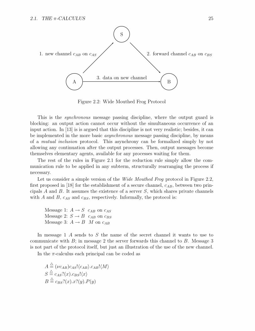
Figure 2.2: Wide Mouthed Frog Protocol
This is the synchronous message passing discipline, where the output guard isblocking: an output action cannot occur without the simultaneous occurrence of aninput action. In [13] is is argued that this discipline is not very realistic; besides, it canbe implemented in the more basic asynchronous message passing discipline, by meansof a mutual inclusion protocol. This asynchrony can be formalized simply by notallowing any continuation after the output processes. Then, output messages becomethemselves elementary agents, available for any processes waiting for them.
The rest of the rules in Figure 2.1 for the reduction rule simply allow the com-munication rule to be applied in any subterm, structurally rearranging the process ifnecessary.
Let us consider a simple version of the Wide Mouthed Frog protocol in Figure 2.2,first proposed in [18] for the establishment of a secure channel, cAB, between two prin-cipals A and B. It assumes the existence of a server S, which shares private channelswith A and B, cAS and cBS, respectively. Informally, the protocol is:
Message 1: A → S cAB on cAS
Message 2: S → B cAB on cBS
Message 3: A → B M on cAB
In message 1 A sends to S the name of the secret channel it wants to use tocommunicate with B; in message 2 the server forwards this channel to B. Message 3is not part of the protocol itself, but just an illustration of the use of the new channel.
In the π-calculus each principal can be coded as
A4= (νcAB)cAS!〈cAB〉.cAB!〈M〉
S4= cAS?(x).cBS!〈x〉
B4= cBS?(x).x?(y).P (y)
26 CHAPTER 2. NOMINAL CALCULI AND CRYPTOGRAPHIC PRIMITIVES
Then, the protocol can be simply formulated as
WMF4= (νcAS)(νcBS)(A | B | S)
If we assume that cAB /∈ fn(P ) ∪ {cAS, cBS} and cAB, cAS, cBS /∈ fn(P (M)) thenthe system has the following computation:
(νcAS)(νcBS)((νcAB)cAS!〈cAB〉.cAB!〈M〉 | cAS?(x).cBS!〈x〉 | cBS?(x).x?(y).P (y))
≡ (νcAS, cBS, cAB)(cAS!〈cAB〉.cAB!〈M〉 | cAS?(x).cBS!〈x〉 | cBS?(x).x?(y).P (y))
→ (νcAS, cBS, cAB)(cAB!〈M〉 | cBS!〈cAB〉 | cBS?(x).x?(y).P (y))
→ (νcAS, cBS, cAB)(cAB!〈M〉 | cAB?(y).P (y))
→ (νcAS, cBS, cAB)(P (M)) ≡ P (M)
Note that in this example the extrusion mechanisms is crucial. Also, this formula-tion is quite abstract, even too abstract if we are interested in its implementation in adistributed environment, since the scope rule is assuming the fresh name does not ap-pear anywhere else. This abstractness motivates the need for a lower-level model, thespi-calculus, which extends the π-calculus with cryptographic primitives (see Section2.3).
Types have been extensively used in the π-calculus to prevent unwanted situations.The first type system for the π-calculus prevented only arity mismatching errors [54].In [63] types are used for resource control, since they restrict the use of channels byassociating them capabilities (whether read only, write only or read&write). Moreover,only data of the correct type can be sent or received over the channels.
In [24] a group creation mechanism is introduced in the language. In this framework,channel names are partitioned into disjoint sets. As a consequence of the existence ofgroups, types allow a finer control of the secrecy of names.
2.2 The Security π-calculus
Next we briefly describe the Security π-calculus [43], a version of the asynchronousπ-calculus in which agents operate in a certain security level. Security levels allows usto address two security issues: resource access control and information flow.
The only difference with respect to the asynchronous π-calculus is the construct
σ�P �
to express that process P is running at a given security level. Here σ is taken from acomplete lattice of security levels SL. Also, channels (the resources in this setting),
2.2. THE SECURITY π-CALCULUS 27
will have an associated set of input/output capabilities, each decorated with a specificsecurity level. These capabilities will be specified by a security policy Γ. For example,if
Γ(e) = {wbot〈B〉, rtop〈A〉}
for some appropriate A and B then low level processes may write to e but only high levelones may read from it. Therefore this is just the security associated with a mailbox.
Resource access control
Resource access errors will be statically detected runtime errors. If Γ associates channeln the highest security level top then the process
c!〈n〉 | bot�c?(x).x?(y).P �
must be ruled out since it evolves, after the communication on c, to process
bot�n?(y).P �
in which a low level process has gained access to the high level resource n. In general,processes at a security level σ should have access to resources at a security level not
greater than σ. These errors will be formalized in terms of a relation PΓ→ err, with
the following basic axioms:
• ρ�a?(x).P � Γ
→ err if for every rσ〈A〉 ∈ Γ(a) it holds σ 6� ρ. That is, if Γ(a) doesnot contain any read capability under ρ
• ρ�a!〈v〉� Γ
→ err if for every wσ〈A〉 ∈ Γ(a) it holds σ 6� ρ. That is, if Γ(a) doesnot contain any write capability under ρ.
Therefore, if Γ(a) = {wσ1〈A〉, rσ2
〈B〉} (again, for some appropriate A and B1) thenρ1
�a?(x).P � | ρ2
�a!〈v〉� does not produce a runtime error with respect to Γ if and only
if σ1 � ρ1 and σ2 � ρ2, that is, both the writing and the reading agent operate ata security level greater or equal than the security levels of the channel for input andoutput actions respectively.
A type system preventing this kind of errors is defined in [43]. There the judgementΓ ` P ensures that P can never violate Γ, as stated in the following
Theorem 1 If Γ ` P then for every context C[ ] such that Γ ` C[P ] and every Q
which occurs during the execution of C[P ], that is C[P ] →∗ Q, we have Q 6Γ→ err
However, since the theorem is restricted to typeable contexts, it is equivalent toprove that typeable terms do not violate the security policy, together with a subjectreduction theorem.
1It must be the case that A is a subtype of B
28 CHAPTER 2. NOMINAL CALCULI AND CRYPTOGRAPHIC PRIMITIVES
Information flow
The security policy we have described does not rule out the possibility of informationleaking indirectly from high to low security levels. For example, let us consider theprocess
top�h?(x). if x = 0 then hl!〈0〉 else hl!〈1〉� | bot
�hl?(z).Q�
where channel h is a high channel and hl is a channel with high-level write access andlow-level read access. This system is typeable with the type system mentioned in theprevious section. However, some information about the value received on the high-levelchannel h can be determined by the low-level process Q (whether it is equal to zero ornot).
A stricter security policy will be needed, that called no read up - no write down.Now, in contrast to the previous policy, high level principals will not be allowed towrite in low level resources.
Absence of information flow will be described in terms of non-interference, andformalized through a special may testing equivalence, P ≈σ
Γ Q that takes into accountsecurity levels. Thus, tests have to satisfy the condition Γ `σ T . This intuitively statesthat, relative to the security policy Γ, processes running at security level σ observe nodifference between the behaviors of P and Q.
We will be interested in processes P such that
P ≈σΓ P | H
for all top-level and σ-free (that cannot reduce their security level to σ) process H.Therefore, high-level processes cannot affect the behaviour of low-level processes.
The same types for resource control, with a slight change, and the same typing rulesare enough to rule out processes that do not fulfill the previous condition. Note thatthe typing system has been used in the definition of non-interference; we are restrictingthe observers of the system to be well-typed.
2.3 The spi-calculus
As we have said before, the π-calculus describes protocols at an abstract level. However,it does not express the cryptographic operations that are commonly used in distributedsystems for the implementation of secure channels. In [6] the spi-calculus is first pre-sented as an extension of the π-calculus with constructs for encryption and decryptionusing symmetric-key cryptography, though it can be easily enhanced to deal also withpublic-key cryptography and hash functions.
The syntax is extended with terms {M}N , that represent the ciphertext obtainedby encrypting the term M under the shared-key N using a shared-key cryptosystemsuch as DES, and a construct for shared-key decryption
case L of {x}N in P

2.3. THE SPI-CALCULUS 29
that attempts to decrypt the term L with the key N . Also, a matching primitive[M is N ]P considered (as well as in some versions of the π-calculus), that behaves likeP only if M and N are the same.
We are assuming in the definition of this new constructs several things about cryp-tography:
• The only way to decrypt an encrypted message is by using the correspondingshared-key.
• An encrypted message does not reveal the shared-key under which it was en-crypted.
• The decryption algorithm knows if the ciphertext was encrypted with the ex-pected key or not (it does not produce nonsense terms by decrypting with thewrong key).
• Principals cannot recognize their own messages.
The operational semantics of the spi-calculus is usually defined through the usualreduction relation and a concretion relation denoted by > (that takes care of localcomputations). The former is defined exactly as in the previous section. Regardingthe latter, its basic axioms are those for decrypting and matching:
case {M}N of {x}N in P > P{x := M}
[M is M ]P > P
Therefore, if the term being decrypted was not ciphered using N , or the comparisonfails, then the processes are stuck.
For example, in process
(νKAB)(cAB!〈{M}KAB〉 | cAB?(x).case x of {y}KAB
in F (y))
the ciphertext {M}KABis sent along a public channel and decrypted on reception. Here
we are assuming that principals agree on the key KAB.Let us consider a cryptographic version of the Wide Mouthed Frog Protocol in Fig-
ure 2.2, closer to the one in [18]2. In this setting, the protocol purpose is that principalsA and B agree on a session key. Informally, the cryptographic protocol is:
2The original one also includes timestamps to avoid replay attacks
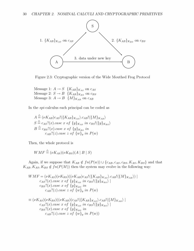
30 CHAPTER 2. NOMINAL CALCULI AND CRYPTOGRAPHIC PRIMITIVES
A B
S
1. {KAB}KASon cAS
3. data under new key
2. {KAB}KBSon cBS
Figure 2.3: Cryptographic version of the Wide Mouthed Frog Protocol
Message 1: A → S {KAB}KASon cAS
Message 2: S → B {KAB}KBSon cBS
Message 3: A → B {M}KABon cAB
In the spi-calculus each principal can be coded as
A4= (νKAB)cAS!〈{KAB}KAS
〉.cAB!〈{M}KAB〉
S4= cAS?(x).case x of {y}KAS
in cBS!〈{y}KBS〉
B4= cBS?(x).case x of {y}KBS
incAB?(z).case z of {w}y in P (w)
Then, the whole protocol is
WMF4= (νKAS)(νKBS)(A | B | S)
Again, if we suppose that KAB /∈ fn(P (w)) ∪ {cAB, cAS, cBS, KAS, KBS} and thatKAB, KAS, KBS /∈ fn(P (M)) then the system may evolve in the following way:
WMF = (νKAS)(νKBS)((νKAB)cAS!〈{KAB}KAS〉.cAB!〈{M}KAB
〉) |cAS?(x).case x of {y}KAS
in cBS!〈{y}KBS〉 |
cBS?(x).case x of {y}KBSin
cAB?(z).case z of {w}y in P (w)
≡ (νKAS)(νKBS)((νKAB)(cAS!〈{KAB}KAS〉.cAB!〈{M}KAB
〉 |cAS?(x).case x of {y}KAS
in cBS!〈{y}KBS〉 |
cBS?(x).case x of {y}KBSin
cAB?(z).case z of {w}y in P (w))

2.3. THE SPI-CALCULUS 31
→ (νKAS, KBS, KAB)(cAB!〈{M}KAB〉 |
case {KAB}KASof {y}KAS
in cBS!〈{y}KBS〉 |
cBS?(x).case x of {y}KBSin
cAB?(z).case z of {w}y in P (w))
> (νKAS, KBS, KAB)(cAB!〈{M}KAB〉 |
cBS!〈{KAB}KBS〉 |
cBS?(x).case x of {y}KBSin
cAB?(z).case z of {w}y in P (w))
→ (νKAS, KBS, KAB)(cAB!〈{M}KAB〉 |
case {KAB}KBSof {y}KBS
incAB?(z).case z of {w}y in P (w))
> (νKAS, KBS, KAB)(cAB!〈{M}KAB〉 |
cAB?(z).case z of {w}KABin P (w))
→ (νKAS, KBS, KAB)(case {M}KABof {w}KAB
in P (w))
> (νKAS, KBS, KAB)P (M) ≡ P (M)
Here the scope extrusion is also essential, but regarding keys, instead of channelnames, since we have transferred the weight of security from channels to keys.
In this context, traditional security properties can be formalized. For example, ifwe call WMF (M) to the version of the protocol in which A(M) sends the message Mto B, we say that the protocol guarantees secrecy of M if WMF (M) ≈ WMF (M ′)for any M and M ′. In fact, such condition holds when ≈ is a may-testing equivalenceand P (M) ≈ P (M ′). Therefore, when the continuation of the protocol guaranteesthe secrecy of M , then also does the protocol. Similarly one can define authenticityproperties.
Types for secrecy
In general, if P is a protocol written in the spi-calculus, it is said to guarantee secrecyon its free variables if for any closed substitutions σ and σ′ it holds Pσ ≈ Pσ′. In [3]type techniques are used to ensure that a protocol guarantees secrecy. Each piece ofdata and each communication channel is labelled either secret or public. Public datacan be communicated to anyone, while secret data should not be leaked (in particular,it should not be sent on public channels). Keys are pieces of data and, as such, arelabelled as Secret or Public (do not confuse with private and public keys in a public-key cryptosystem). Also, a type Any is used in the formalism to denote arbitrary data,that subsumes both Secret and Public. Thus, a subtype notion is introduced, T <: Sthat holds whenever T equals S or S equals Any.

32 CHAPTER 2. NOMINAL CALCULI AND CRYPTOGRAPHIC PRIMITIVES
The basic judgments of the type system will have the form Γ ` P , that will be de-fined with the help of judgments Γ ` M : T for terms, with T ∈ {Public, Secret, Any}and Γ ` P for processes. The typing rules are simply formalizing the following ideas:The result of encrypting data with a public-key has the same classification as the data,while the ciphertext obtained by encrypting with a secret-key can be made public;concerning channels, only public data can be sent on public channels, while all kinds ofdata may be sent on private channels. However, encrypted messages (encrypted withprivate keys) and messages sent on private channels will have a special format in orderto differentiate the levels of the data they contain. Thus, only messages of the form(M1,M2,M3) can be sent on private channels, where M1 is secret, M2 is of type Anyand M3 is public. Also, ciphertexts will have the special format (indistinguishable forthe observer) {M1,M2,M3, n} where each Mi is as before and n is a confounder, thatcan only be used for the encryption of (M1,M2,M3), but only once, so as not to repeatciphertexts, thus avoiding dictionary attacks. We will write n : T :: {M1,M2,M3, n}N
in an environment Γ if, relative to Γ name n can be used as a confounder only for thatexpression and has level T . We will simply write n : T if n is not meant to be used asa confounder. Of course, variables cannot be used as confounders and, therefore, onlyexpressions like x : T may appear in environments. For example if K is a secret keythen the process
(νn) ∗ c?(x1, x2, x3).d!〈{x1, x2, x3, n}K〉
that can use the same confounder for many different encrypts will be ruled out, whileprocess
c?(x1, x2, x3).(νn) ∗ d!〈{x1, x2, x3, n}K〉
that uses n only once as a confounder (although the resulting ciphertext can be sentmany times) will be permitted.
Some of the rules that take into account these considerations are the rule for sendingon a private channel
Γ ` M : SecretΓ ` M1 : Secret Γ ` M2 : Any Γ ` M3 : Public
Γ ` PΓ ` M !〈M1,M2,M3〉.P
or the rule for encryption
Γ ` M1 : Secret Γ ` M2 : Any Γ ` M3 : PublicΓ ` N : Secret n : T :: {M1,M2,M3, n}N in Γ
Γ ` {M1,M2,M3, n}N : Public
However, if the channel is public it may only send public values
Γ ` M : PublicΓ ` M1 : Public, . . . ,Mk : Public
Γ ` PΓ ` M !〈M1, . . . ,Mk〉.P

2.3. THE SPI-CALCULUS 33
and, if the key is public, then the ciphertext may not be public:
Γ ` M1 : T, . . . , Γ ` Mk : T Γ ` N : Public(with T = Public if k = 0)
Γ ` {M1, . . . ,Mk}N : T
The rule for name restriction infers the type of the created name needed to typethe rest of the process:
Γ, n : T :: L ` P
Γ ` (νn)P
Finally, we will consider the rule for the matching construct [M is N ]P , thatbehaves like P if M equals N . The comparison of names implies a leak of information.Therefore, the typing rule will forbid such construct if any of the names involved hastype Any:
for T,R ∈ {Public, Secret}Γ ` M : T Γ ` N : R Γ ` P
Γ ` [M is N ]P
Note that all the type system allows for names or variables of type Any is to besent on private channels or encrypted with secret keys on public channels: they cannotbe sent on public channels, since they could be secret, they cannot be used to encrypt,since they could be public and they cannot be compared, to avoid implicit flows.
The typing system is meant to protect parameters of level Any relying on dyamicallygenerated names of level Secret, when at first only variables of type Any and publicchannels appear on the environment. For instance, let us consider the following process
(νK)(νm)(νn)c!〈{m,x, 0, n}K〉
and an environment Γ containing x : Any and c : Public. Since channel c is public,the message sent on it must also be public and, since x has type Any, that can onlyhappen if the key K is private, m is public and n is an appropriate confounder.
The substitutions used in the secrecy theorem must satisfy certain conditions: Wewrite Γ ` σ when σ(x) is a closed term (without variables) such that fn(σ(x)) ⊆ dom(Γ)for every x ∈ dom(Γ). Then the main theorem is stated as follows:
Theorem 2 Given an environment Γ such that only variables of level Any and namesof level Public are in dom(Γ), if we have that Γ ` σ, Γ ` σ′ and Γ ` P then Pσ ' Pσ′,that is, P preserves the secrecy of its free variables.
We can reconsider the Wide Mouthed Frog protocol of Figure 2.3. The special for-mat of encrypted messages obliges us to rewrite the agents in a more complicated way,though its computations are the same:
A(v)4= (νKAB)(νCA)(νC ′
A)cAS!〈{KAB, ∗, ∗, CA}KAS〉.cAB!〈{∗, v, ∗, C ′
A}KAB〉

34 CHAPTER 2. NOMINAL CALCULI AND CRYPTOGRAPHIC PRIMITIVES
S4= (νCB)cAS?(x).case x of {x1, x2, x3, x4}KAS
in cBS!〈{x1, ∗, ∗, CB}KBS〉
B4= cBS?(x).case x of {x1, x2, x3, x4}KBS
incAB?(z).case z of {y1, y2, y3, y4}x1
in P (y2)
where ∗ is an arbitrary message of appropriate level (not necessarily the same for allthe occurrences of ∗). Again, the protocol is
WMF (v) = (νKAS)(νKBS)(A(v) | S | B)
Now we consider an environment Γ satisfying Γ(v) = Any and Γ(cij) = Public forall i, j. It can be proven (although we do not show here the corresponding derivation)that if Γ ` P (v) then Γ ` WMF (v). If P (v) has a known particular form that weknow typeable then we get the following
Result 5 The protocol WMF (M) guarantees the secrecy of M
To conclude with the section, we comment on some other techniques for provingsecurity properties of spi-like languages. In [5] a type system for secrecy is presentedthat can treat in a generic way many cryptographic operations. In [11] a symbolic oper-ational semantics for the language is developed, that is proved to be consistent with theoriginal semantics. This symbolic treatment is the basis for a trace analysis method,that can be automatically carried out. This method is used to prove that WMFguarantees secrecy and authentication (in some sense). In [12] an enriched labelledtransition system is developed to investigate tractable proof methods for two equiva-lences, namely may-testing and barbed equivalence, used on the definition of severalsecurity properties. Finally, in [9] both the π-calculus and the spi-calculus are extendedwith two primitives that guarantee entity authentication and message authentication(credit and responsibility respectively, in the terminology of [2]), using techniques from[31]. The idea is to have protocols that are secure by construction. Then, a notion ofimplementation of those primitives in the original calculus is developed in [10].
2.4 The Distributed π-calculus: Dπ
In this section we describe a distributed variant of the π-calculus, called Dπ [41], anda type system based on the notion of capacities, that rules out resource access errorsin this framework. When we have an open system we need to ensure that resources areprotected against non-authorized accesses. These unauthorized accesses are capturedconsidering a tagged version of the language.
Being an extension of the π-calculus, resources in the first version of Dπ are nothingbut channels. Agents will be located threads of the form k
�P �, where k is a locality
identifier and P is an ordinary term of the π-calculus extended with primitives formovement and for creation of localities. Communication in Dπ is local, that is, agents

2.4. THE DISTRIBUTED π-CALCULUS: Dπ 35
Names Values
e::=k locality u, v::=bv base values| a channel | e name
| x variablePatterns | u@v localized name
X,Y ::=x variable | (u1, . . . , un) tuple| X@z localized pattern| (X1, . . . , Xn) tuple
Processes Systems
P,Q::=. . . . . . M,N ::=0 empty| go u.P movement | M | N composition| (νe : E)P restriction | (νke : E)N restriction
| k�P � agent
Figure 2.4: Syntax of the Dpi
must be in the same locality in order to communicate. Therefore, channels will beassociated to localities. By default, if a channel is sent then the receiver takes it asbelonging to the locality it lies on now. Otherwise, we will use the construction a@k,meaning “channel a at location k”.
An error will occur when using a channel without the capability to do so. We aregoing to present a type system that prevents these errors. Both the formalization oferrors and the type system are based on ideas from [63].
2.4.1 Syntax and semantics
The syntax of the language is defined in Figure 2.4. The dots stand for the usual prim-itives of the π-calculus, that is, termination, composition, replication, input, outputand conditional. A primitive go for movement is introduced and created names canbe channels but also localities. The possible messages are locations, channels, locatedchannels and tuples. Therefore we need as patterns not only variables and tuples butalso localized patterns. The main syntactic category is that of system N, which intu-itively consists of a set of agents running in parallel. As we said before, an agent is alocated thread, k
�P �.
As in the Ambient Calculus that we will later study, the semantics of Dπ is definedthrough a structural equivalence ≡ and a reduction relation →, defined in Figure 2.5and Figure 2.6 repectively. The relation ≡ is the least equivalence that is closed undercomposition and restriction, satisfies the commutative monoid laws for composition and0 and the axioms in Figure 2.5. These rules allow the spawning of new agents (S-SPLIT

36 CHAPTER 2. NOMINAL CALCULI AND CRYPTOGRAPHIC PRIMITIVES
(S-EXTR) M | (νke : E)N ≡ (νke : E)(M | N) if e 6∈ fn(M)(S-COPY) k
�∗P � ≡ k
�P � | k
�∗P �
(S-NEW) k�(νe : E)P � ≡ (νke : E)k
�P � if e 6= k
(S-SPLIT) k�P | Q� ≡ k
�P � | k
�Q�
(S-GARB1) (νke : E)0 ≡ 0(S-GARB2) k
�stop� ≡ 0
Figure 2.5: Structural equivalence of the Dpi
(R-GO) `�go k.P � → k
�P �
(R-COMM) k�a!〈v〉P � | k
�a?(X).Q� → k
�P � | k
�Q{X := v}�
(R-EQ1) k�if u = u then P else Q� → k
�P �
(R-EQ2) k�if u = v then P else Q� → k
�Q� if u 6= v
(R-STR)N → N ′
(νe)N → (νe)N ′N → N ′
M | N → M | N ′N ≡ M M → M ′ M ′ ≡ N ′
N → N ′
Figure 2.6: Reduction relation of the Dpi
and S-COPY), garbage collection (S-GARB1 and S-GARB2) and scope extrusion (S-EXTR and S-NEW). Note that when a name restriction is extruded out of an agent(S-NEW), we have to record the location at which the name was created.
In Figure 2.6 the reduction relation (among closed terms) is defined. Rule (R-GO)accounts for agent movement. This rule causes the topology of localities of every systemto be plain, in the sense that every agent can go to any location from every location,provided it knows its name. Note that in rule (R-COMM), the communicating agentsmust be co-located and share a channel at that location. The rest of the rules are thesame as in the π-calculus (extending the match primitive for the else case).
2.4.2 Errors and types
Resource access errors will be articulated by means of capacity types. Each agent willhave associated a set of capacities, that is, a set of known localities, each of them witha set of known channels. This is formalized by means of environments, that are finitemappings from locality identifiers to locality types (see Figure 2.7). For instance, if anagent has its capacities determined by Γ, having Γ(k) = loc{a : res〈T 〉, b : res〈T ′〉},then it knows locality k and two channels at k, namely a and b, that can be used toexchange messages of type T and T ′ respectively. The types of possible exchanged

2.4. THE DISTRIBUTED π-CALCULUS: Dπ 37
LType: K ::= loc{a : A}, ai distinct loc{a : A, b : B} <: loc{a : A}RType: A ::= res〈T 〉AType: E ::= A | K | B A <: AVType: T ::= A | B B <: B
| (A1, . . . , An)@K A@K <: A@L if K <: L
| (T1, . . . , Tn) S <: T if ∀i : Si <: Ti
Figure 2.7: Types and subtyping in the Dpi
values are those of tuples, channels, localized channels and base values, ranged by B.We will write res〈K〉 as a shorthand for res〈()@K〉 and, if Γ(k) = loc{. . . , a : A, . . .}we will write Γ(k, a) = A.
A notion of subtyping is also defined in Figure 2.7. If we see location types as setsof capabilities, then subtyping can be expressed as reversed inclusion:
K <: L iff K ⊇ L
Here we take the order on channels and base values to be trivial. <: is a partial orderon types that induces a partial meet operator u. This ordering and the operator extendcomponent-wise to environments.
To indicate that an agent k�P � has capacities determined by Γ we will write k
�P �Γ.
In this setting, capacities can only be acquired, never lost. There are two ways in whichan agent can get new capacities:
1. The agent can create a resource and then it owns the capacity to use it. This isachieved by means of a modification of rule S-NEW:
(ST -NEW) k�(νe : E)P �Γ ≡ (νke : E)k
�P �Γ,{ke:E} if e 6∈ fn(Γ) ∪ {k}
where Γ, {ke : E} stands for the extension of Γ with e at location k, which is onlydefined if k 6∈ dom(Γ) or e : E 6∈ Γ(k).
2. An agent can transmit a capacity to another agent via communication. The re-ceiver acquires the capacity to use the received channels with the type determinedby that of the input variable:
(ST -COMM) k�a!〈v〉P �Γ | k
�a?(X : T ).Q�∆ → k
�P �Γ | k
�Q{X := v}�∆u{kv:T}
where {kv : T} is the environment in which the names in v are assigned the typesin T at k. For example:
{`(a, b@k) : (A,B@loc{c : C})} = {` : loc{a : A}, k : loc{c : C, b : B}}

38 CHAPTER 2. NOMINAL CALCULI AND CRYPTOGRAPHIC PRIMITIVES
Note that what is being done is developing a tagged version of the language toexplicitly deal with capabilities [41]. The rest of the structural and reduction rulessimply transmit the capabilities along the computation. For instance, the rule formovement now becomes
(ST -GO) `�go k.P �Γ → k
�P �Γ
and the ones for splitting an agent and spawning a new agent are
(ST -SPLIT) k�P | Q�Γ ≡ k
�P �Γ | k
�Q�Γ
and
(ST -COPY) k�∗P �Γ ≡ k
�P �Γ | k
�∗P �Γ
In fact, these rules restrict the semantics of the language (for instance, now twoagents can only be merged if they have the same capacities). However, in practice, thethree described structural rules for the tagged language are meant to be used left toright. Indeed, some later versions of the Dπ substitute these structural rules for thecorresponding reduction ones [42, 40].
Now that we know what capacities each agent possesses and how can they gain newcapacities, we describe how they could violate the permissions they own. obj denotesthe function on channel types such that obj(res〈T 〉) = T and Γk(v) denotes the leasttype, if any, which the typing environment Γ can assign to the value v at location k3.For example, if
Γ(k, a) = A, Γ(k, b) = B and Γ(k) = loc{c : C}
thenΓ`((a, b)@k)) = (A,B)@loc{c : C}
Intuitively, a runtime error occurs whenever an agent attempts to use a namecontrary to the capabilities it has acquired for that name. There are three ways inwhich this can happen:
1. The sender tries to forge capabilities, that is, the sender tries to send a value vthrough a channel a that requires more capabilities than available at v.
`�c!〈a〉�Γ | `
�c?(x : A).x!〈k〉�∆ → `
�stop�Γ | `
�a!〈k〉�∆,{`a:A} → err
Γ → ` : loc
{
a : Ac : res〈A〉
(A = res〈loc{b : B}〉)
∆ →
{
` : loc{c : res〈A〉}k : loc
3Defined by induction on the structure of v:
Γk(a) = Γ(k, a) Γk(v@`) = Γ`(v)@Γ(`) Γk(v1, . . . , vn) = (Γk(v1), . . . ,Γk(vn))

2.4. THE DISTRIBUTED π-CALCULUS: Dπ 39
In this example, the first communication does not go wrong. By means of it thereceiver agent has gained the capability to use channel a to send localities thatpossess at least a channel b. However, now he is using that new channel to senda location k for which he does not know any channel. Thus, he is trying to forgethe permission to use b at k.
2. The receiver tries to forge capabilities, that is, the receiver may not expect avalue that exceeds its capacities for the channel it is sent through.
`�c!〈a〉.a!〈k〉�Γ | `
�c?(x : A).x?(z : loc{b : B, d : D}).Q�∆ →
`�a!〈k〉�Γ | `
�a?(z : loc{b : B, d : D}).Q�∆,{`a:A} → err
Γ →
{
` : loc{a : A, c : res〈A〉} (A = res〈loc{b : B}〉)k : loc{b : B, d : D}
∆ → ` : loc{c : res〈A〉}
As in the previous case, by means of the first communications the receiver obtainspermission to use channel a to exchange localities with a channel b. However, inthe second communication it is trying to receive a locality with two channels, band d.
3. The sender and the receiver do not agree on the use of the common channel, thatis, the sender view of the channel does not fulfill the receiver’s expectations.
`�a!〈k〉�Γ | `
�a?(x : T ).P �∆ → err
Γ →
{
` : loc{a : res〈loc{b : B}〉}k : loc{b : B}
∆ → ` : loc{a : res〈loc{b : B, c : C}〉}
Here the receiver expects to receive localities equipped with two channels, but itonly receives a locality with one channel.
Runtime errors are formally defined in Figure 2.8. The basic rules have been il-lustrated through the previous examples, that corresponded to rules E-SND, E-RCVand E-COMM respectively. The rest of the rules simply transmit errors to the wholeprocess. Therefore, two agents trying to communicate
k�a!〈v〉P �Γ | k
�a?(X : T ).Q�∆
do not cause a runtime error only if the following constraints are satisfied:
Γk(v) <: obj(Γ(k, a)) <: obj(∆(k, a)) <: T

40 CHAPTER 2. NOMINAL CALCULI AND CRYPTOGRAPHIC PRIMITIVES
(E-SND) k�a!〈v〉P �Γ→ err if Γk(v) 6<: obj(Γ(k, a))
(E-RCV) k�a?(X : T ).Q�∆→ err if obj(∆(k, a)) 6<: T
(E-COMM) k�a!〈v〉P �Γ | k
�a?(X : T ).Q�∆→ err if obj(Γ(k, a)) 6<: obj(∆(k, a))
(E-STR)N → err
(νe)N → errN → err
N | M → errN ≡ M M → err
N → err
Figure 2.8: Runtime errors in the Dpi
Let us consider the following system:
`�(νa : A)c!〈a〉 a!〈k〉�Γ | `
�c?(x : A). x?(z : loc{b : B, d : D}).Q�∆ (2.1)
where Γ = {` : loc{c : res〈A〉}, k : K}, ∆ = {` : loc{c : res〈A〉}} andA = res〈loc{b : B}〉. This system is structurally equivalent to
((ν`a : A))(`�c!〈a〉 a!〈k〉�Γ′ | `
�c?(x : A). x?(z : loc{b : B, d : D}).Q�∆)
where Γ′ = {` : loc{a : A, c : res〈A〉}, k : K}.
Two consecutive communications between the agents occur. However, only thesecond one produces a resource access error. Let us see it in detail:
For the first communication to be correct it suffices to see that the chain of con-straints we have seen holds (using Γ′). In fact, here the chain is simply A <: A <: A <: A.After the first communication the system becomes
(ν`a : A)(`�a!〈k〉�Γ′ | `
�a?(z : loc{b : B, d : D}).Q�∆′)
where ∆′ = {` : loc{a : A, c : res〈A〉}}. However, now we can apply rule E-RCV toget an error, since the type of the expected value exceeds the capabilities of channel a,that is,
obj(∆′(`, a)) = loc{b : B} 6<: loc{b : B, d : D}
If the receiver had not tried to forge capabilities then the second communicationwould have not produced any error either:
`�(νa : A)c!〈a〉 a!〈k〉�Γ | `
�c?(x : A). x?(z : loc{b : B}).Q�∆ →∗ (ν`a : A)`
�Q{z := k}�∆′′
with ∆′′ = {` : loc{a : A, c : res〈A〉}, k : loc{b : B}}
Of course, if Q tries to use channel d afterwards then the error will occur at thatmoment, since the agent has not acquired the permission to use it.

2.4. THE DISTRIBUTED π-CALCULUS: Dπ 41
2.4.3 Type system
In this section a type system that guarantees that no runtime errors occur is described.The primary judgments will be of the form Γ ` N , meaning that the term N is well-typed with respect to the environment Γ, which provides a type for every free identifierin N . Intuitively, it can be interpreted as the initial global capabilities of all the agentsappearing in N . We use auxiliary judgments for threads and values. Judgments havethe form Γ `w P for processes, indicating that the thread P is well-typed to run atlocation w, with w ∈ dom(Γ), and Γ `w u : T for values, meaning that value u hastype T at w relative to environment Γ.
The typing rules are those given in Figure 2.9. They are quite easy to understand.For example, rule N-RUN states that k
�P � is a well-typed agent if its thread is well-
typed at location k. Rule T-GO says that go u.P is a correct thread to be executed atlocation w if u is indeed a location and P is a correct thread to be executed at locationu. In rule V-DEP it is necessary that u can be typed with a location type and v asa tuple of channels. There is no explicit subsumption rule, but rule V-UNIV has thesame effect: if Γ(k) = loc{a : A, b : B} then it holds Γ ` k : loc{a : A, b : B}, but alsoΓ ` k : loc{a : A}, Γ ` k : loc{b : B} and Γ ` k : loc.
The most important rules are T-W and T-R, the ones that control communications.In order to apply rule T-W it is necessary that the types of the channel and the messagesent through that channel are the same. If the environment gives more capacities tothe sent values that to the channel we can always type the value with the same typeas the channel (rule V-UNIV). Similarly, T-R obliges the annotated type of the inputvariable to be the same as the type of the input channel. However, since T is fixed bythe syntax of the process and there is no subtyping on channels we cannot reason as inrule T-W and, therefore, both types must be identical. This restriction can be solvedby introducing subtyping also in channels.
Let us consider again the Example 2.1. One of its threads evolved to
`�a?(z : loc{b : B, d : D}).Q�
According to the previous rules this process is not typeable under the environment∆′ = {` : loc{a : A, c : res〈A〉}}. To do so, according to rule (T-R) we should derive∆′ `` a : res〈loc{b : B, d : D}〉, but ∆′(`, a) = res〈loc{b : B}〉 6= res〈loc{b : B, d : D}〉.
So far we have described the type system for the original calculus. However, thetype system can be extended to the tagged language simply by a slight modification ofrule N-RUN. The rest of the rules remain as in the untagged version of the language.We use the symbol instead of `, when we are dealing with tagged processes. Thenew rule, (NT -RUN), is
Γ <: ∆ ∆ `k P
Γ k�P �∆
The first condition verifies that the capacities specified by ∆ are consistent withthe global types in Γ. The second requirement states that P must be typed only with

42 CHAPTER 2. NOMINAL CALCULI AND CRYPTOGRAPHIC PRIMITIVES
Values
(V-UNIV)Γ(u) <: K
Γ `w u : K
(V-LOCAL)Γ(w) <: loc{u : A}
Γ `w u : A
(V-DEP)Γ `w u : K Γ `u v : B
Γ `w v@u : B@K
(V-TUP)Γ `w ui : Ti (∀i)
Γ `w u : T
Threads
(T-W)Γ `w u : res〈T 〉Γ `w v : TΓ `w P
Γ `w u!〈v〉P
(T-R)Γ `w u : res〈T 〉fv(X) ∩ fv(Γ) = ∅Γ, {wX : T} `w Q
Γ `w u?(X : T ).Q
(T-EQ)Γ `w u : TΓ `w v : TΓ `w PΓ `w Q
Γ `w if u = v then P else Q
(T-GO)Γ `w u : locΓ `u P
Γ `w go u.P
(T-NEW)e 6∈ fn(Γ)Γ, {we : E} `w P
Γ `w (νe : E)P
(T-STR)Γ `w PΓ `w Q
Γ `w stop, P | Q, ∗P
Systems
(N-RUN)Γ `k P
Γ ` k�P �
(N-NEW)e 6∈ fn(Γ)Γ, {ke : E} `w N
Γ ` (νke : E)N
(N-STR)Γ ` MΓ ` N
Γ ` 0,M | N
Figure 2.9: Typing rules for the Dpi

2.4. THE DISTRIBUTED π-CALCULUS: Dπ 43
the resources it is allowed to use. For instance, it is impossible to derive
Γ k�a!〈 〉�{...,k:loc{c:C},...}
even if Γ(k) includes channel a, since a is not known by the agent at location k.In [41] a subject reduction theorem is proven for the two type systems. Also, it is
proved that well-typed tagged processes do not produce runtime errors.
Theorem 3 If N is a tagged system and Γ N then N 6→ err.
This, together with subject reduction, gives us as a corollary the following
Theorem 4 If Γ N and N →∗ N ′ then N ′ 6→ err.
In the case in which the Example 2.1 did not try to forge the capability to usechannel d it holds that if ∆′′ ` Q{z := k} then the whole system can be typed and,therefore, it produces no errors. Note that the fact that Q can be typed under ∆′′
means in particular that it does not attempt to use channel d. If not, as we have saidbefore, it would produce an error and, indeed, Q could not have been typed.
Now it remains the problem of relating both the untagged and the tagged versionof the language. In [41] a function tagΓ is defined. This function takes an untaggedterm and returns the set of tagged terms that can be safely typed using environmentsgreater than Γ. If the term is not typeable under Γ then it returns the empty set. Thedefinition of tagΓ is simultaneously done for all the Γ’s, by induction on the structureof the term. The main cases are those of agents and name restriction:
tagΓ(k�P �) = {k
�P �∆ | Γ <: ∆ and ∆ `k P}
tagΓ((νke : E)N) = (νke : E)tagΓ,{ke:E}(N)
Following this definition, well-typed systems can be regarded as tagged systems inwhich tags can be inferred. Since the definition is based on the rules for typing taggedsystems, it is trivial that
M ∈ tagΓ(N) ⇒ Γ M
and then we have the final
Theorem 5 If M ∈ tagΓ(N) and M →∗ M ′ then M ′ 6→ err
However, it is not possible to talk about errors produced by non typeable systems,that is, if Γ 6` N then tagΓ(N) = ∅ and we do not have a model to describe the possibleerrors the system may produce.
We think that a way to express the property in the original calculus is needed. Infact, tagged systems can be derived from the corresponding untagged one by a simpleinspection of its history, except for the initial permissions. Thus, if we have a functiontag (that will be deterministic for us), that gives the initial tags of the system, then
44 CHAPTER 2. NOMINAL CALCULI AND CRYPTOGRAPHIC PRIMITIVES
the history of the process contains enough information to infer the rest of the tags and,therefore, errors become an implicit property of the original language. For instance, ifour tag is such that
tag(`�(νa : A)c!〈a〉 a!〈k〉� | `
�c?(x : A). x?(z : loc{b : B, d : D}).Q�) =
`�(νa : A)c!〈a〉 a!〈k〉�Γ | `
�c?(x : A). x?(z : loc{b : B, d : D}).Q�∆
with A, Γ and ∆ as in Example 2.1, then we can say that system
`�(νa : A)c!〈a〉 a!〈k〉� | `
�c?(x : A). x?(z : loc{b : B, d : D}).Q�
is erroneous (or evolves to an erroneous system). A possible solution would be toinitially annotate agents only with the permissions to use channels they have createdthemselves. In Chapter 6 we will try to shed some light on these ideas.

Chapter 3
Ambient Calculus
In this chapter we will introduce the language we will mainly use throughout this workto model mobile systems, the Ambient Calculus [25], that explicitly considers mobilityprimitives, unlike the π-calculus. We focus on this process algebra instead of othersimilar languages (like the Dπ described in Chapter 2) due to its simplicity and, at thesame time, expresiveness.
Ambients will be the main entities of this model. An ambient is a place limited by aboundary where computations take place. Mobile ambients encompass, within a singleframework, both agents and the environments where agents interact, while focusing onthe notions of locations, of mobility (of agents and environments themselves) and ofauthorization to move [20]. Computational ambients are hierarchically structured, soas to not abstract from the path needed to follow to arrive the destination. Agentsare confined to ambients and ambients move under the control of agents, allowing themovement of nested environments, that also include data and live computation.
Ambients have a name (not necessarily unique, different ambients may have thesame name) and a content (basically a parallel composition of sequential processesand subambients). They can move into their sibling ambients or exit their enclosingambient, moving with them all its subcomponents. Ambients can also dissolve theboundary of its subambients, so that the processes contained in the opened ambientnow belong to the opener ambient. Opening of ambients is the basic mechanism ofambient interaction. Next we define the syntax and the semantics of the language.
3.1 Syntax and semantics
In Figure 3.1 the syntax for the Ambient Calculus with communication primitivesis presented. We will consider two disjoint sets, N = {m,n, . . .} for names andV = {x, y, . . .} for variables, and a special symbol ε. We will denote Id = N ∪ V,cap(Id) = {in N, out N, open N | N ∈ Id} and capmv(Id) = {in N, out N | N ∈ Id}.If A is a set we will denote A∗ the set of paths formed over elements of A, that is, thesmallest set such that ε ∈ A∗, A ⊆ A∗ and M,N ∈ A∗ ⇒ M.N ∈ A∗.
The general shape of an ambient is:
45
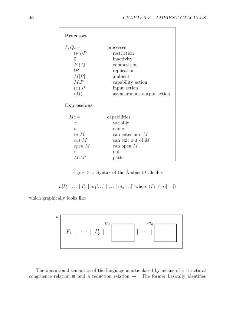
46 CHAPTER 3. AMBIENT CALCULUS
Processes
P,Q::= processes(νn)P restriction0 inactivityP | Q composition!P replicationM [P ] ambientM.P capability action(x).P input action〈M〉 asynchronous output action
Expressions
M ::= capabilitiesx variablen namein M can enter into Mout M can exit out of Mopen M can open Mε nullM.M ′ path
Figure 3.1: Syntax of the Ambient Calculus
n[P1 | . . . | Pp | m1[. . .] | . . . | mq[. . .]] where (Pi 6= nj[. . .])
which graphically looks like
n
m1 mq
P1 | . . . | Pp | |. . .|
The operational semantics of the language is articulated by means of a structuralcongruence relation ≡ and a reduction relation →. The former basically identifies
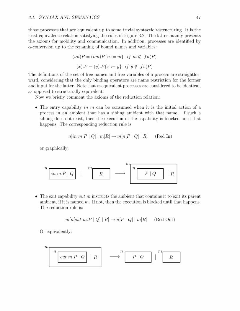
3.1. SYNTAX AND SEMANTICS 47
those processes that are equivalent up to some trivial syntactic restructuring. It is theleast equivalence relation satisfying the rules in Figure 3.2. The latter mainly presentsthe axioms for mobility and communication. In addition, processes are identified byα-conversion up to the renaming of bound names and variables:
(νn)P = (νm)P{n := m} if m 6∈ fn(P )
(x).P = (y).P{x := y} if y 6∈ fv(P )
The definitions of the set of free names and free variables of a process are straightfor-ward, considering that the only binding operators are name restriction for the formerand input for the latter. Note that α-equivalent processes are considered to be identical,as opposed to structurally equivalent.
Now we briefly comment the axioms of the reduction relation:
• The entry capability in m can be consumed when it is the initial action of aprocess in an ambient that has a sibling ambient with that name. If such asibling does not exist, then the execution of the capability is blocked until thathappens. The corresponding reduction rule is:
n[in m.P | Q] | m[R] → m[n[P | Q] | R] (Red In)
or graphically:
in m.P | Q | R P | Q | R−→n m
mn
• The exit capability out m instructs the ambient that contains it to exit its parentambient, if it is named m. If not, then the execution is blocked until that happens.The reduction rule is:
m[n[out m.P | Q] | R] → n[P | Q] | m[R] (Red Out)
Or equivalently:
out m.P | Q | R P | Q | R−→
mn mn

48 CHAPTER 3. AMBIENT CALCULUS
Structural congruence
P ≡ Q ⇒ (νn)P ≡ (νn)Q (Struct Res)P ≡ Q ⇒ P | R ≡ Q | R (Struct Par)P ≡ Q ⇒ !P ≡!Q (Struct Repl)P ≡ Q ⇒ n[P ] ≡ n[Q] (Struct Amb)P ≡ Q ⇒ M.P ≡ M.Q (Struct Action)P | Q ≡ Q | P (Struct Par Comm)(P | Q) | R ≡ P | (Q | R) (Struct Par Assoc)!P ≡ P |!P (Struct Repl Par)(νn)(νm)P ≡ (νm)(νn)P (Struct Res Res)(νn)(P | Q) ≡ P | (νn)Q if n /∈ fn(P ) (Struct Res Par)(νn)(m[P ]) ≡ m[(νn)P ] if n 6= m (Struct Res Amb)P | 0 ≡ P (Struct Zero Par)(νn)0 ≡ 0 (Struct Zero Res)!0 ≡ 0 (Struct Zero Repl)P ≡ Q ⇒ (x).P ≡ (x).Q (Struct Input)ε.P ≡ P (Struct ε)(M.M ′).P ≡ M.M ′.P (Struct Path)
Reduction
n[in m.P | Q] | m[R] → m[n[P | Q] | R] (Red In)m[n[out m.P | Q] | R] → n[P | Q] | m[R] (Red Out)open n.P | n[Q] → P | Q (Red Open)(x).P | 〈M〉 → P{x := M} (Red Comm)P → Q ⇒ (νn)P → (νn)Q (Red Res)P → Q ⇒ n[P ] → n[Q] (Red Amb)P → Q ⇒ P | R → Q | R (Red Par)P ′ ≡ P, P → Q,Q ≡ Q′ ⇒ P ′ → Q′ (Red ≡)
Figure 3.2: Operational Semantics of the Ambient Calculus

3.1. SYNTAX AND SEMANTICS 49
• An open n capability can be consumed when we have an ambient named n in thesame ambient where the capability appears. If used, that subambient disappearsand its content in the following belongs to the surrounding ambient. Otherwise,the action is blocked. Thus, the rule for opening an ambient is:
open n.P | n[Q] → P | Q (Red Open)
That is:
−→open n.P P | Qn
Q|
The only way in which two processes located in different ambients can interactis by means of an open action. However, the rule above has been consideredtoo dangerous, both from the side of the opening ambient (it gains full accessto the resources in the opened ambient, but at the same time some potentiallymalicious processes could be admitted in the ambient) and from the side of theambient being opened (it may not want to be opened now). In Chapter 5 somealternative proposals for process interaction will be presented.
• Communication in the Ambient Calculus is local and asynchronous. Such asyn-chrony is modelled by means of the asynchronous output action 〈M〉 which actslike a post-it on a blackboard, waiting for some input action to consume it. Thecommunication rule is:
(x).P | 〈M〉 → P{x := M} (Red Comm)
In the original paper [25] a pure ambient calculus is first presented, withoutprimitives for communication, in order to focus in the main novelty of mobileambients, mobility. As a matter of fact this simple calculus turns out to beTuring-complete, and therefore any communication mechanism could be encodedin it. However, the existence of explicit communication primitives is essential forreadability.
Remark: For simplicity, in the syntax definition ambient names and capabilitiesbelong to the same syntactic category. As a consequence the syntax allows the con-struction of meaningless processes such as n.P or in n[P ]. Later these terms will beruled out by the type system that we will discuss.

50 CHAPTER 3. AMBIENT CALCULUS
3.2 Security in the Ambient Calculus
The security problems considered within the mobile ambients framework are thosethat arise as a misuse of the primitives, not those that are a consequence of a badimplementation of primitives. That is, we assume that an attacker has at its disposalonly the primitives of the Ambient Calculus.
The Ambient Calculus deals with security concerns in a rather high-level way, with-out the use of primitives for encryption and decryption. It is based on the knowledgeof ambient names by processes and therefore the basic mechanism that is involved isthat of name restriction, in the style of π-calculus.
A restricted name cannot be used outside its scope. If anyhow the name appearsthere, then we are referring to different names, even if we call them in the same way.However, α-conversion can be used to avoid this confusion, and in this way it is reflectedthe fact that the restricted name cannot be known, in principle, out of the restrictedterm. By means of the extrusion rule we can augment the scope of the restriction froma parallel component to the whole parallel composition, provided the restricted namedoes not appear in the other components:
P | (νn)Q ≡ (νn)(P | Q) if n 6∈ fn(P )
As said before, if process P above does have n as a free name and we want P andQ to interact we can always apply α-conversion:
P | (νn)Q = P | (νm)Q{n := m} ≡ (νm)(P | Q{n := m}) if m 6∈ fn(P ) ∪ fn(Q)
For example, if n and m agree on a key k, then the ambient m can allow theentrance of n though, at first, no one knows its name:
(νk) ( n[open k.P ] | (νm) m[k[out m.in n.in m] | Q] ) (3.1)
Ambient m can be regarded as a firewall that agent n wants to cross. If n,m and kare pairwise distinct and m 6∈ fn(P ) then the process above can evolve in the followingway (with no need to use α-conversion):
(νk) ( n[open k.P ] | (νm)m[k[out m.in n.in m] | Q] )
→ (νk)(n[open k.P ] | (νm)(m[Q] | k[in n.in m]))
≡ (νk,m)(n[open k.P ] | k[in n.in m] | m[Q])
→ (νk,m)(n[open k.P | k[in m]] | m[Q])
→ (νk,m)(n[P | in m] | m[Q])
→ (νk,m)m[Q | n[P ]]
The above mechanism can be used to guarantee agent authentication, to ensurefreshness of messages by means of nonces or to model shared-key cryptography.
The following example can be found in [25]:
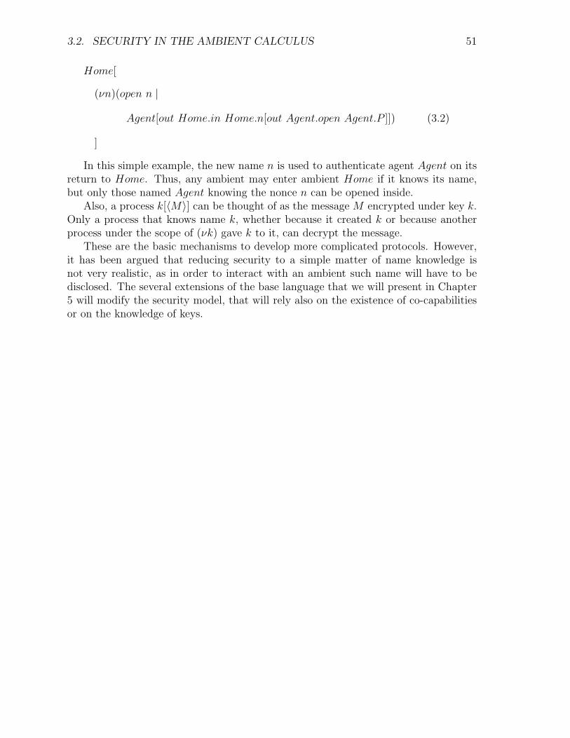
3.2. SECURITY IN THE AMBIENT CALCULUS 51
Home[
(νn)(open n |
Agent[out Home.in Home.n[out Agent.open Agent.P ]]) (3.2)
]
In this simple example, the new name n is used to authenticate agent Agent on itsreturn to Home. Thus, any ambient may enter ambient Home if it knows its name,but only those named Agent knowing the nonce n can be opened inside.
Also, a process k[〈M〉] can be thought of as the message M encrypted under key k.Only a process that knows name k, whether because it created k or because anotherprocess under the scope of (νk) gave k to it, can decrypt the message.
These are the basic mechanisms to develop more complicated protocols. However,it has been argued that reducing security to a simple matter of name knowledge isnot very realistic, as in order to interact with an ambient such name will have to bedisclosed. The several extensions of the base language that we will present in Chapter5 will modify the security model, that will rely also on the existence of co-capabilitiesor on the knowledge of keys.

52 CHAPTER 3. AMBIENT CALCULUS

Chapter 4
Types for the Ambient Calculus
In this chapter we will discuss the papers on types for the Ambient Calculus by Cardelliet al [26, 21, 22, 23]. The experience with Java has already shown the utility oftypes for mobile code, specially when dealing with security properties. In general, inevery type system that we will consider, restrictions on ambient names are imposed bythe programmer (either by means of name declaration or in the environment for freenames). The typing rules will transmit these restrictions to the rest of the system, thismeaning that in order to type certain subterms we will have to take into account theserestrictions. Therefore, as far as we have more and more restrictions, the systems willbe harder to type.
Therefore, in the whole chapter we will assume that every ambient name has a typeassociated (either in its declaration or in the environment). However, when we do notwant to impose any special restriction on an ambient it is natural to let the typingsystem infer a proper type in a way that the process becomes typeable. This speciallyapplies to types that do not express particular intentions of the programmer on the useof an ambient, but technical conditions in order to have more powerful typing results(see ST-types in Chapter 5).
Several notions of run-time errors will be defined in this chapter: one that detectscommunication errors, and two that detect communication, mobility and ambient-opening errors. The three type systems defined will be proven to rule out such errors.An alternative approach would have been to keep those topics separated (communi-cation, mobility and ambient-opening), thus defining a different kind of error for eachone of them and also a different type system for each of them, since they are indeedcompletely orthogonal.
4.1 Exchange types
In [26] the first type system for the Ambient Calculus is presented. Its main purposeis to avoid meaningless processes. Such processes may arise after some undesired
53

54 CHAPTER 4. TYPES FOR THE AMBIENT CALCULUS
Exchange type
T ::=Shh no exchangeW1 × . . . × Wk tuple exchange
Message type
W ::=Amb[T ] ambients that may contain exchanges of type TCap[T ] capabilities that may unleash exchanges of type T
Figure 4.1: Exchange Types
communication interactions. For instance, the process
(x).x[P ] | 〈n〉 | (y).y.Q | 〈open n〉
may evolve to
n[P ] | open n.Q
but also to
(open n)[P ] | n.Q
In order to avoid these meaningless terms1 the idea is to restrict the type of com-munications within each ambient, thus defining the exchange types. To be more exact,we associate types to names and not to individual ambients: any ambient with thesame name will be typed in the same way. These types will not only specify whetherambients or capabilities are exchanged, but also what kind of ambients (including theinformation that can be exchanged inside them) or what kind of capabilities. Thelatter is necessary in order to know what kind of exchanges could they unleash, whenopening an ambient. For example, for the process m[open n.Q | n[P ]] to control theexchanges inside m we need to know if exchanges in process P are compatible withthose in Q. This is, of course, recursively applied.
The ambient calculus that we will study in this section is a slight extension of theone we have seen in the previous section. It allows tuple communication, what providesa more expressive type system.
There are two kinds of exchange types: one for no exchange, Shh, and the otherfor tuple exchange, where each component will be an ambient type or a capacity type,as formalized in Figure 4.1.
The only differences on the syntax with respect to the original calculus lie on com-munication constructs:
1In fact they are only meaningless at the intuitive level. Formally they just include useless blockedsubterms.
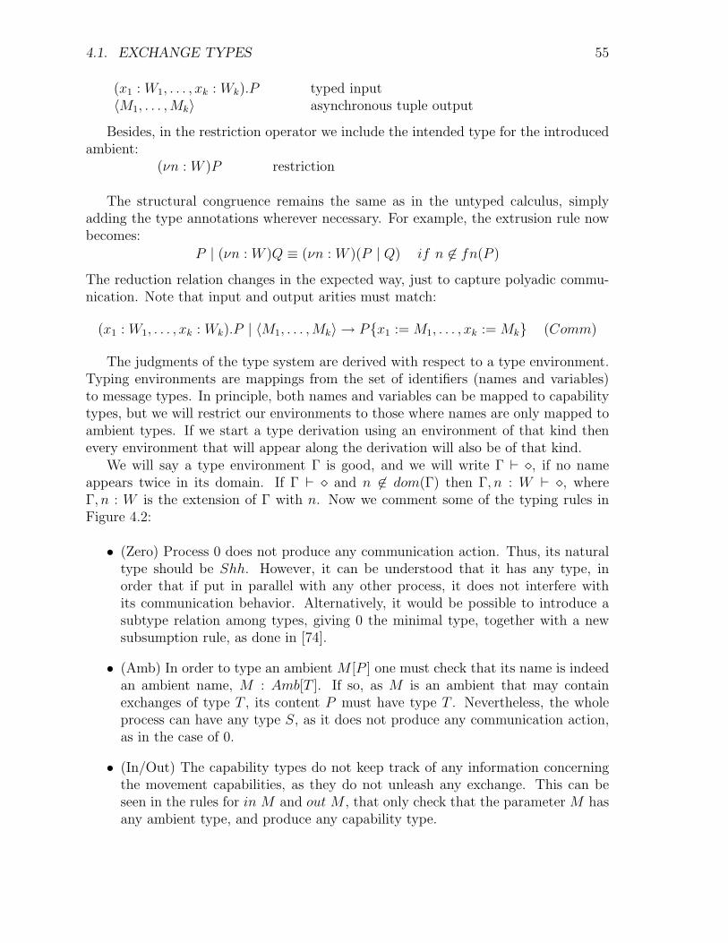
4.1. EXCHANGE TYPES 55
(x1 : W1, . . . , xk : Wk).P typed input〈M1, . . . ,Mk〉 asynchronous tuple output
Besides, in the restriction operator we include the intended type for the introducedambient:
(νn : W )P restriction
The structural congruence remains the same as in the untyped calculus, simplyadding the type annotations wherever necessary. For example, the extrusion rule nowbecomes:
P | (νn : W )Q ≡ (νn : W )(P | Q) if n 6∈ fn(P )
The reduction relation changes in the expected way, just to capture polyadic commu-nication. Note that input and output arities must match:
(x1 : W1, . . . , xk : Wk).P | 〈M1, . . . ,Mk〉 → P{x1 := M1, . . . , xk := Mk} (Comm)
The judgments of the type system are derived with respect to a type environment.Typing environments are mappings from the set of identifiers (names and variables)to message types. In principle, both names and variables can be mapped to capabilitytypes, but we will restrict our environments to those where names are only mapped toambient types. If we start a type derivation using an environment of that kind thenevery environment that will appear along the derivation will also be of that kind.
We will say a type environment Γ is good, and we will write Γ ` �, if no nameappears twice in its domain. If Γ ` � and n 6∈ dom(Γ) then Γ, n : W ` �, whereΓ, n : W is the extension of Γ with n. Now we comment some of the typing rules inFigure 4.2:
• (Zero) Process 0 does not produce any communication action. Thus, its naturaltype should be Shh. However, it can be understood that it has any type, inorder that if put in parallel with any other process, it does not interfere withits communication behavior. Alternatively, it would be possible to introduce asubtype relation among types, giving 0 the minimal type, together with a newsubsumption rule, as done in [74].
• (Amb) In order to type an ambient M [P ] one must check that its name is indeedan ambient name, M : Amb[T ]. If so, as M is an ambient that may containexchanges of type T , its content P must have type T . Nevertheless, the wholeprocess can have any type S, as it does not produce any communication action,as in the case of 0.
• (In/Out) The capability types do not keep track of any information concerningthe movement capabilities, as they do not unleash any exchange. This can beseen in the rules for in M and out M , that only check that the parameter M hasany ambient type, and produce any capability type.
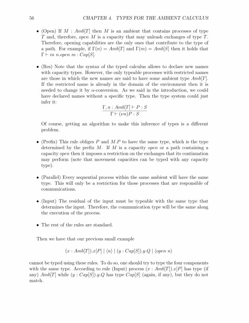
56 CHAPTER 4. TYPES FOR THE AMBIENT CALCULUS
• (Open) If M : Amb[T ] then M is an ambient that contains processes of typeT and, therefore, open M is a capacity that may unleash exchanges of type T .Therefore, opening capabilities are the only ones that contribute to the type ofa path. For example, if Γ(n) = Amb[T ] and Γ(m) = Amb[S] then it holds thatΓ ` in n.open m : Cap[S].
• (Res) Note that the syntax of the typed calculus allows to declare new nameswith capacity types. However, the only typeable processes with restricted namesare those in which the new names are said to have some ambient type Amb[T ].If the restricted name is already in the domain of the environment then it isneeded to change it by α-conversion. As we said in the introduction, we couldhave declared names without a specific type. Then the type system could justinfer it:
Γ, n : Amb[T ] ` P : S
Γ ` (νn)P : S
Of course, getting an algorithm to make this inference of types is a differentproblem.
• (Prefix) This rule obliges P and M.P to have the same type, which is the typedetermined by the prefix M . If M is a capacity open or a path containing acapacity open then it imposes a restriction on the exchanges that its continuationmay perform (note that movement capacities can be typed with any capacitytype).
• (Parallel) Every sequential process within the same ambient will have the sametype. This will only be a restriction for those processes that are responsible ofcommunications.
• (Input) The residual of the input must be typeable with the same type thatdetermines the input. Therefore, the communication type will be the same alongthe execution of the process.
• The rest of the rules are standard.
Then we have that our previous small example
(x : Amb[T ]).x[P ] | 〈n〉 | (y : Cap[S]).y.Q | 〈open n〉
cannot be typed using these rules. To do so, one should try to type the four componentswith the same type. According to rule (Input) process (x : Amb[T ]).x[P ] has type (ifany) Amb[T ] while (y : Cap[S]).y.Q has type Cap[S] (again, if any), but they do notmatch.

4.1. EXCHANGE TYPES 57
(Exp n) (Path)
Γ ` � Γ(n) = W
Γ ` n : W
Γ ` Mi : Cap[T ] i = 1, 2
Γ ` M1.M2 : Cap[T ]
(Empty) (In/Out) (Open)
Γ ` �Γ ` ε : Cap[T ]
Γ ` M : Amb[T ]
Γ ` in/out M : Cap[S]
Γ ` M : Amb[T ]
Γ ` open M : Cap[T ]
(Prefix) (Amb) (Res)
Γ ` M : Cap[T ] Γ ` P : T
Γ ` M.P : T
Γ ` M : Amb[T ] Γ ` P : T
Γ ` M [P ] : S
Γ, n : Amb[T ] ` P : S
Γ ` (νn : Amb[T ])P : S
(Zero) (Par) (Repl)
Γ ` �Γ ` 0 : T
Γ ` Pi : T i = 1, 2
Γ ` P1 | P2 : TΓ ` P : TΓ `!P : T
(Input) (Output)
Γ, x1 : W1, . . . , xk : Wk ` P : W1 × . . . × Wk
Γ ` (x1 : W1, . . . , xk : Wk).P : W1 × . . . × Wk
Γ ` Mi : Wi i = 1..k
Γ ` 〈M1, . . . ,Mk〉 : W1 × . . . × Wk
Figure 4.2: Typing rules for Exchange Types

58 CHAPTER 4. TYPES FOR THE AMBIENT CALCULUS
4.1.1 Communication runtime errors
In [26] only the intuitive meaning of types is described, but it is a simple exerciseto formalize these meanings. For it, we can define binary relations ↓Amb, ↓Pref and↓Msg that look for the occurrences of term M as an ambient, a prefix or a message,respectively. Then, we get the collection of axioms and rules in Figure 4.3, withσ ∈ {Amb, Pref,Msg}. Using these relations we formalize in Figure 4.4 the firstnotion of error that we will consider, err1. It can be considered to be a syntacticerror, that arises from the use of two different kind of entities (names and capacities)in the same syntactic category. The definition of err1 attempts to detect the erroras soon as possible, in the sense that it looks in every subcomponent of the process,although without considering variables, since we do not know, in principle, what willthey be substituted for. For example, in the case of a prefixed process, even if thefirst capacity is not erroneous it still may detect an error in forthcoming capabilities.This is also the case for input processes. Note that, having the rule for the inputconstruct, we must deal with processes that may contain free variables. For instance,(x : W ).x[P ] | 〈in n〉 ↓Amb x and (x : W ).x[P ] | 〈in n〉 ↓Msg in n , but since x ∈ Id andin n ∈ cap(Id), we cannot derive (x : W ).x[P ] | 〈in n〉 → err1. However, it can evolveto (in n)[P ], which verifies that (in n)[P ] ↓Amb in n with in n 6∈ Id and, therefore,(in n)[P ] → err1.
If we suppose that P 6→ err1 and Q 6→ err1 then we can easily verify that
(x : W ).x[P ] | 〈n〉 | (y : W ′).y.Q | 〈open n〉err1
n[P ] | open n.Q
(open n)[P ] | n.Q
err1
err1
Note that this is true no matter what W and W ′ are, even if they are capabilityand ambient types respectively. For example, if P does not produce an error of thiskind, neither does (x : Cap[T ]).x[P ] | 〈n〉 or its immediate successor n[P ].
In the first place, typed processes do not cause an error:
Theorem 6 If Γ ` P : T then P 6→ err1
This result can easily be proved considering that processes that cause an error arebasically those that contain a subterm of the form (cap N)[P ], 〈cap (cap′ N)〉, n.P orcap (cap′ N).P . These processes are not typeable nor any process that contains them(in our type system every subterm must be typed in order to type the whole term). Asubject reduction theorem for exchange types is proven in [26]. Using it we get our
Theorem 7 If Γ ` P : T and P →∗ Q then Q 6→ err1

4.1. EXCHANGE TYPES 59
M.P ↓Pref M M [P ] ↓Amb M 〈M〉 ↓Msg Mi
P ↓σ M
N [P ] ↓σ M
P ↓σ M
N.P ↓σ M
P ↓σ M
(x : W ).P ↓σ M
P ↓σ M
(νn : W )P ↓σ M
P ↓σ M
P | Q ↓σ M
Q ↓σ M
P | Q ↓σ M
P ↓σ M
!P ↓σ M
Figure 4.3: Showing an ambient name, a prefix or a message
P ↓Amb M M 6∈ IdP → err1
P ↓Pref M M 6∈ (V ∪ cap(Id))∗
P → err1
P ↓Msg M M 6∈ Id ∪ cap(Id)∗
P → err1
Figure 4.4: Rules for errors of first class

60 CHAPTER 4. TYPES FOR THE AMBIENT CALCULUS
Γ(n) = Amb[Shh]
n[(x1 : W1, . . . , xk : Wk)P | 〈M1, . . . ,Mk〉 | Q]Γ→ err2
Γ(n) = Amb[W ′1 × . . . × W ′
r] k 6= r
n[(x1 : W1, . . . , xk : Wk)P | 〈M1, . . . ,Mk〉 | Q]Γ→ err2
Γ(n) = Amb[W ′1 × . . . × W ′
k] ∃i.Wi 6= W ′i
n[(x1 : W1, . . . , xk : Wk)P | 〈M1, . . . ,Mk〉 | Q]Γ→ err2
Γ(n) = Amb[W1 × . . . × Wk] ∃i.Γ 6` Mi : Wi
n[(x1 : W1, . . . , xk : Wk)P | 〈M1, . . . ,Mk〉 | Q]Γ→ err2
PΓ,n:W−→ err2
(νn : W )PΓ→ err2
P ≡ Q QΓ→ err2
PΓ→ err2
PΓ→ err2
P | QΓ→ err2
PΓ→ err2
n[P ]Γ→ err2
P → err1
PΓ→ err2
Figure 4.5: Rules for errors of second class
Remark: The assumption that there are no names in Γ associated to capability typesis needed to avoid situations like the following. Let us suppose that Γ(n) = Cap[Shh],then Γ ` n.0 : Shh but this process is considered to be meaningless.
We can include in the definition of erroneous states the communication policy speci-fied by a typing environment Γ. Since now run-time errors depend on the environment,
we will write PΓ→ err2 if it can be derived from the rules in Figure 4.5.
The definition of err2 is quite flexible, in the sense that errors of this type onlyappear when an effective communication can take place immediately. That is why thearities of the input and the output constructs in its rules always match. For instance,it does not hold that
(νn : Amb[Shh])n[〈n〉]Γ→ err2
nor
(νn : Amb[Shh])n[〈n, n〉 | (x : W )P ]Γ→ err2
since no actual communication occurs (in the first case because there is no readingprocess and in the second because arities are not the same). Actually, it would beeasy to extend the typing system to consider in ambients a set of blackboards, onefor each arity, instead of the single blackboard considered so far. Also, errors are notpropagated when a process is guarded by a prefix or an input. For example, it is nottrue that
(νn : Amb[Shh])n[in m.(x).P | 〈M〉] | m[Q]Γ→ err2

4.1. EXCHANGE TYPES 61
but the process evolves to
(νn : Amb[Shh])m[n[(x).P | 〈M〉] | Q]Γ→ err2
As opposed to the previous one, now errors can appear as a consequence of badinteraction between components. Thus, an error occurs whenever an illegal communi-cation may take place. If the ambient is defined to be silent then every exchange in itis considered to be illegal. On the contrary, if an ambient has type Amb[W1× . . .×Wk]and an exchange takes place inside it, three conditions are needed so it does not pro-duce an error: the arity of the exchange must match the arity of the ambient type, thetype of the ambient must match the variable’s annotations and the type of the outputmessages must match the ambient type.
Also, note that not only the policy specified by the typing environment, but alsothe restrictions in the declarations are considered. For example, if we denote by φ theenvironment with empty domain then
(νn : Amb[Shh])n[(νm : Amb[Shh])〈open m〉 | (x : Cap[Amb[Shh]]).P ]φ
−→ err2
can be derived since we also have
n[〈open m〉 | (x : Cap[Amb[Shh]])P ]Γ→ err2
where Γ = {n : Amb[Shh],m : Amb[Shh]}.
Remark: Note that a type judgement appears as premise in one of the rules for err2.One has to be careful when defining a notion of error depending on the type system,so as not getting circular results.2 However, in this case, the judgment is a conditionon an expression, that can be checked by simply looking it up in the environment.
As we have now that Γ ` P : T implies P 6Γ→ err2, then we can restate the safety
property using err2 instead of err1:
Theorem 8 If Γ ` P : T and P →∗ Q then Q 6Γ→ err2.
To conclude the section, let us say that rules PREFIX and INPUT state that thetopic of conversation within an ambient does not change along the computation. Thisrestriction makes untypeable processes like
(νn : Amb[Real])((x : Int).open n.(y : Real).P | 〈3〉 | n[〈3.5〉])
although no process Q reachable from it verifies Q → err1. As we have said before,[7], [8] and [38], among other works, try to overcome this restriction.
2This happens if, for example, we take as erroneous processes those that cannot be typed

62 CHAPTER 4. TYPES FOR THE AMBIENT CALCULUS
4.1.2 Multiple arity types
As we have said before, it is straightforward to extend the type system in the previoussection to deal with exchanges of different arities within the same ambient, since theydo not interfere with each other. We could have exchange types T as partial mappingsfrom natural numbers to message tuples, such that:
• dom(T ) is a finite set
• For each k ∈ dom(T ) it is T (k) = W1 × . . . × Wk
The role of the exchange type Shh of the previous section is here played by aritiesnot in the domain of T . Then we can define a partial meet operator u satisfying:
• T u T ′ defined ⇔ ∀k ∈ dom(T ) ∩ dom(T ′) it holds T (k) = T ′(k)
• (T u T ′)(k) =
{
T (k) if k ∈ dom(T )T ′(k) if k ∈ dom(T ′)
The corresponding type system is a simple generalization of that in the previoussection. Rules for 0, ambients, prefixes, replication and capabilities remain exactly thesame. However, the rule for parallel composition now becomes
Γ ` Pi : Ti
Γ ` P1 | P2 : T1 u T2
that assumes the meet of types is defined. It states that a parallel composition canonly be typed if the exchanges in each component are compatible. If exchanges of thesame arity can occur in both components then they have to be of the same type, butexchanges of different arities can safely take place. The rules for inputs and outputsare
T (k) = W1 × . . . × Wk Γ, x1 : W1, . . . , xk : Wk ` P : T
(x1 : W1, . . . , xk : Wk).P : T
andT (k) = W1 × . . . × Wk Γ ` Mi : Wi ∀i ∈ {1, . . . , k}
Γ ` 〈M1, . . . ,Mk〉 : T
respectively. They check that for the corresponding arity the type associated to theprocess matches the type of the exchange. In particular, if k is not in the domain ofΓ, neither outputs nor inputs of that arity can be typed.
The previous types can be embedded in the new type system. If we denote byΦ the empty type (the one with empty domain) then we can define tr(Shh) = Φand tr(W1 × . . . × Wk) = T , where dom(T ) = {k} and T (k) = W1 × . . . × Wk for ex-change types. Concerning message types, tr(Amb[T ]) = Amb[tr(T )] and analogouslytr(Cap[T ]) = Cap[tr(T )], which extends component-wise to environments. For pro-cesses, the only not simply structural case is tr((νn : W )P ) = (νn : tr(W ))tr(P ).

4.2. TYPES FOR MOBILITY AND OPENING CONTROL 63
k 6∈ dom(Γ(n))
n[(x1 : W1, . . . , xk : Wk)P | 〈M1, . . . ,Mk〉 | Q]Γ→ err′2
Γ(n) = Amb[T ] T (k) = W ′1 × . . . × W ′
k ∃i.Wi 6= W ′i
n[(x1 : W1, . . . , xk : Wk)P | 〈M1, . . . ,Mk〉 | Q]Γ→ err′2
Γ(n) = Amb[T ] T (k) = W1 × . . . × Wk ∃i.Γ 6` Mi : Wi
n[(x1 : W1, . . . , xk : Wk)P | 〈M1, . . . ,Mk〉 | Q]Γ→ err′2
PΓ,n:W−→ err′2
(νn : W )PΓ→ err′2
P ≡ Q QΓ→ err′2
PΓ→ err′2
PΓ→ err′2
P | QΓ→ err′2
PΓ→ err′2
n[P ]Γ→ err′2
P → err1
PΓ→ err′2
Figure 4.6: Rules for errors of second class with multiple arities
Then it holds that if Γ ` P : T with the type system in the previous section thentr(Γ) ` tr(P ) : tr(T ) can also be derived with the multiple arity type system.
A subject reduction theorem can also be proven for this type system. Also, err′2,the notion of error corresponding to err2 in this new setting can be defined, as it is donein Figure 4.6. It holds that typed terms do not produce errors of this new kind and,therefore, we can conclude that terms reachable from a typeable term do not producethis kind of errors either.
It is true that this extension does not give us any extra expressive power, since everytype of the new form can be encoded with the types in the previous section, simply byconsidering tuples that are long enough to cope with every component of each arity.However, this encoding would produce quite complicated processes. Although theseideas could also be followed in the following, we prefer to stick to the original works,for the sake of readability.
4.2 Types for mobility and opening control
In the previous section we have presented a simple type system for the ambient calculusthat removes meaningless terms. To do this, it needs to control the communicationactions in each ambient. However, as we have said before, mobility and not communi-cation is the main issue of the Ambient Calculus. Therefore, from the point of view ofsecurity, the considered types are not too informative.
In a mobile agent system some entities are supposed to be mobile (mobile agents)but some others are supposed to be stationary agents or servers. Also, some aresupposed to be openable (such as packets) and some are not. In [21] a type system is

64 CHAPTER 4. TYPES FOR THE AMBIENT CALCULUS
described to formalize these intentions. Types will restrict the behavior of ambients,more specifically, whether ambients with a certain name can move and whether theycan be opened by its enclosing ambient. We have to specify these restrictions whennames are created.
For example, we would like that the process
a[p[out a.in b.〈M〉]] | b[open p.(x : W ).P ]
would be typeable under the restrictions that a and b cannot move or be opened.
4.2.1 Type syntax and typing rules
Next we formally describe the new type system. First, in Figure 4.7 the syntax ofmobility types is defined.
Y ::= locking annotation• locked◦ unlocked
Z ::= mobility annotationsy mobileY immobile
W ::= message typeAmbY [ZT ] ambient nameCap[ZT ] capability
T ::= exchange typeShh no exchangeW1 × . . . × Wk tuple exchange
Figure 4.7: Mobility Types
• AmbY [ZT ] is the type of ambients whose locking and mobility attributes are Yand Z, respectively, and that allow exchanges of type T . If Y = • then theambient cannot be opened by any process; if Z = Y then the ambient can nevermove. Exchange type T is the same as in the former type system.
• Cap[ZT ] is the type of a capability that unleashes communications of type T andcan produce a movement iff Z =y. The occurrence of a movement capacityimplies the mobility of the process it prefixes.

4.2. TYPES FOR MOBILITY AND OPENING CONTROL 65
• ZT is the type of processes with exchanges of type T and that can produce somemovement iff Z =y, in which case, it transmits its mobility effects to the rest ofthe parallel components that could appear.
Now let us describe the most interesting typing rules. These are rules Exp In andExp Out
Γ ` M : AmbY [ZT ]
Γ ` in M : Cap[yT ′]
Γ ` M : AmbY [ZT ]
Γ ` out M : Cap[yT ′]
They introduce the mobility effects. Movement capabilities do not unleash anyexchange, as formalized by the fact that they can unleash any exchange. These capa-bilities can only appear inside mobile ambients, as derived from rules Amb and Prefix:
Γ ` M : AmbY [ZT ] Γ ` P : ZT
Γ ` M [P ] :Z′
T ′
Γ ` M : Cap[ZT ] Γ ` P :Z T
Γ ` M.P :Z T
Indeed, if M is declared to be immobile in Γ this forces us to try to type its contentalso as immobile, which is not possible if one of its sequential processes has an in orout prefix.
Rule (Exp Open) states that an open M capability is only typeable if M is anambient that can be opened. In that case, the exchanges and the mobility effectsunleashed by open M are those allowed by the ambient M :
Γ ` M : Amb◦[ ZT ]
Γ ` open M : Cap[ ZT ]
The rest of the rules are simple.
Let us remind our firewall Example 3.1 in Section 3.2. Now we are imposing thatm is an ambient that cannot be moved or opened:
S = (νk : Amb◦[ yShh])
( n[open k.P ] | (νm : Amb•[ YShh])m[k[out m.in n.in m] | Q] )
If we assume that
Γ(n) = AmbY [ yShh]
Γ′ ` P : yShh Γ′ ` Q : YShh
where Γ′ = Γ, k : Amb◦[ yShh] then the whole process can be typed. On the one hand,we have:

66 CHAPTER 4. TYPES FOR THE AMBIENT CALCULUS
Γ′ ` n : AmbY [ yShh]
Γ′ ` k : Amb◦[ yShh]
Γ′ ` open k : Cap[yShh] Γ′ ` P : yShh
Γ′ ` open k.P : yShh
Γ′ ` n[open k.P ] : ZT
If we denote Γ′′ = Γ′,m : Amb•[ YShh] we can obtain, by applying rule (Prefix) threetimes, that Γ′′ ` out m.in n.in m : yShh. Then, on the other hand, we can derive:
Γ′′ ` m : Amb•[ YShh]
Γ′′ ` k : Amb◦[ yShh] out m.in n.in m : yShh
Γ′′ ` k[out m.in n.in m] :Y Shh Γ′′ ` Q : YShh
Γ′′ ` k[out m.in n.in m] | Q : YShh
Γ′′ ` m[k[out m.in n.in m] | Q] : ZT
Γ′ ` (νm : AmbY [ yShh]) m[k[out m.in n.in m] | Q] : ZT
So that Γ ` S : ZT , and we can type the system under the restriction indicating thatambient m is immobile.
However, it could happen that an immobile ambient wants to open a mobile am-bient that has already consumed all its movement capabilities. This situation is notallowed by the present typing system. Let us consider again the agent authenticationexample (3.2)
Home[
(νn)(open n |
Agent[out home.in home.n[out Agent.open Agent.P ]])
]
If we want to type this process with respect to an environment Γ satisfying therestriction Γ(Home) = Amb•[YT ] we need to type any process in Home as YT , inparticular the process open n. If we look at rule (Exp Open) we see that in order todo that n should have been declared with type Amb◦[YT ], which is impossible, sinceambient n contains movement capacities. This type system also fails when trying totype the system
a[p[out a.in b.〈M〉]] | b[open p.(x : W ).P ]
when a and b are declared as immobile. Several solutions to relax these limitations canbe found in the literature. We will study one of them in the next section and anotherone in Chapter 5.
In [21] a subject reduction theorem for mobility types is proven.To finish with this section, let us say that mobility types are a conservative extension
of exchange types. Indeed, we can embed them in the following way:
• tr(Amb[T ]) = Amb◦[yT ]
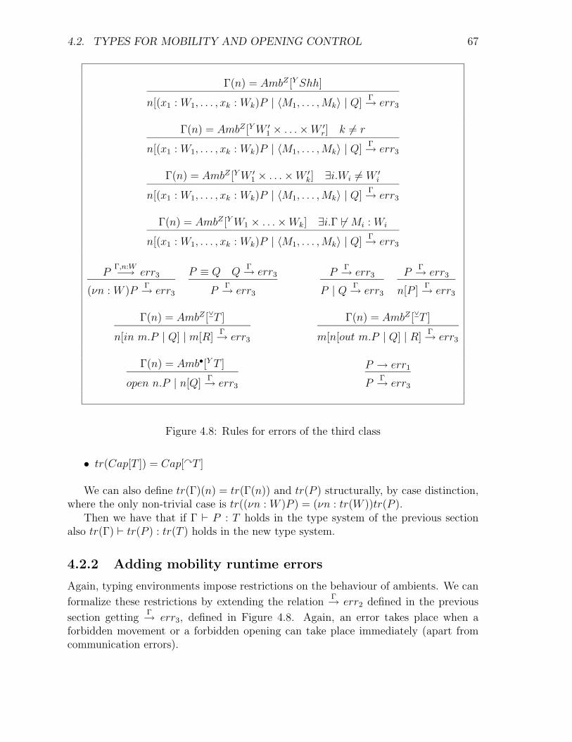
4.2. TYPES FOR MOBILITY AND OPENING CONTROL 67
Γ(n) = AmbZ [Y Shh]
n[(x1 : W1, . . . , xk : Wk)P | 〈M1, . . . ,Mk〉 | Q]Γ→ err3
Γ(n) = AmbZ [Y W ′1 × . . . × W ′
r] k 6= r
n[(x1 : W1, . . . , xk : Wk)P | 〈M1, . . . ,Mk〉 | Q]Γ→ err3
Γ(n) = AmbZ [Y W ′1 × . . . × W ′
k] ∃i.Wi 6= W ′i
n[(x1 : W1, . . . , xk : Wk)P | 〈M1, . . . ,Mk〉 | Q]Γ→ err3
Γ(n) = AmbZ [Y W1 × . . . × Wk] ∃i.Γ 6` Mi : Wi
n[(x1 : W1, . . . , xk : Wk)P | 〈M1, . . . ,Mk〉 | Q]Γ→ err3
PΓ,n:W−→ err3
(νn : W )PΓ→ err3
P ≡ Q QΓ→ err3
PΓ→ err3
PΓ→ err3
P | QΓ→ err3
PΓ→ err3
n[P ]Γ→ err3
Γ(n) = AmbZ [YT ]
n[in m.P | Q] | m[R]Γ→ err3
Γ(n) = AmbZ [YT ]
m[n[out m.P | Q] | R]Γ→ err3
Γ(n) = Amb•[Y T ]
open n.P | n[Q]Γ→ err3
P → err1
PΓ→ err3
Figure 4.8: Rules for errors of the third class
• tr(Cap[T ]) = Cap[yT ]
We can also define tr(Γ)(n) = tr(Γ(n)) and tr(P ) structurally, by case distinction,where the only non-trivial case is tr((νn : W )P ) = (νn : tr(W ))tr(P ).
Then we have that if Γ ` P : T holds in the type system of the previous sectionalso tr(Γ) ` tr(P ) : tr(T ) holds in the new type system.
4.2.2 Adding mobility runtime errors
Again, typing environments impose restrictions on the behaviour of ambients. We can
formalize these restrictions by extending the relationΓ→ err2 defined in the previous
section gettingΓ→ err3, defined in Figure 4.8. Again, an error takes place when a
forbidden movement or a forbidden opening can take place immediately (apart fromcommunication errors).

68 CHAPTER 4. TYPES FOR THE AMBIENT CALCULUS
Now it can be proven that if Γ ` P : T holds then P 6Γ→ err3. Applying subject
reduction we obtain as usual corresponding correctness theorem:
Theorem 9 If Γ ` P : T and P →∗ Q then Q 6Γ→ err3
In particular, no ambient declared as immobile will ever move and no ambientdeclared as not openable will ever be opened. We can apply the theorem to Example3.1 to conclude that m will not ever move or be opened.
4.2.3 Objective moves
One way to relax the previous type system is to consider objective moves, with theintroduction of the primitive go N.M [P ]. This process moves the ambient M [P ] asspecified by the N capability, and has M [P ] as its continuation. Such movementis called objective because ambient M [P ] is moved from the outside, in contrast tomovements caused by a process N.Q running inside M , that in this context we callsubjective moves. Note that ambient M does not become active until it has been moved.We add to the calculus the structural rule
go ε.M [P ] ≡ M [P ]
and the following reductions:
go(in m.N).n[P ] | m[Q] → m[go N.n[P ] | Q] (Red Go In)
m[go(out m.N).n[P ] | Q] → go N.n[P ] | n[Q] (Red Go Out)
Objective moves can be easily encoded with objective moves by the following trans-lation:
go N.M [P ] = (νk)k[N.M [out k.P ]] where k 6∈ fn(N.M [P ])
However, due to their specificity, objective moves allow a more refined type system. Anew attribute for objective moves is added to ambient types, which now have the formAmbY Z [Z
′
T ]. This new attribute is ignored except in the rule Proc Go:
Γ ` N : Cap[Z′
S] Γ ` M : AmbY Z′
[ZT ] Γ ` P :Z T
Γ ` go N.M [P ] :Z′′
T ′′
where it is verified that if M is an ambient that cannot be objectively moved (Z ′ =y)then N is a capability that produces no movement (N = ε). Note that the previousencoding of the new primitive is only typeable in the previous type system if we allowambient M to be mobile (see rule Prefix). Now it is possible to type the new constructif we restrict M to be subjectively immobile.

4.2. TYPES FOR MOBILITY AND OPENING CONTROL 69
As an example, let us try to type our example of the sending of a packet. We canrewrite it by using objective moves as follows:
a[go (out a.in b).p[〈M〉]] | b[open p.(x : W ).P ]
If we assume that Γ(a) = Amb•Y[YShh], Γ(p) = Amb◦y[YW ], Γ(b) = Amb•Y[YShh],Γ ` M : W and Γ, x : W ` P :Y W we get the typing
Γ ` a[go (out a.in b).p[〈M〉]] | b[open p.(x : W ).P ] :Y Shh
We could also rewrite our Example 3.2 using the new primitives:
Home[(νn : Amb◦y[YShh])
(open n | go(out Home.in Home).Agent[go(outAgent).n[open Agent.P ]])
]
that can be typed under an environment Γ such that Γ(Home) = Amb•Y[YShh],Γ(Agent) = Amb◦y[YShh] and Γ, n : Amb◦y[YShh] ` P :Y Shh.
In the following derivation we omit the attribute Shh that appears in every typejudgment and we write
Q′ = go(out Agent).n[open Agent.P ]
Q = go(out Home.in Home).Agent[Q′] and
Γ′ = Γ, n : Amb◦y[YShh].
Γ′ ` Agent : Amb◦y[Y]
Γ′ ` out Agent : Cap[y] Γ′ ` n : Amb◦y[Y]
Γ′ ` Agent : Amb◦y[Y]
Γ′ ` open Agent : Cap[Y] Γ′ ` P :Y
open Agent.P :Y
Γ′ ` Q′ = go(outAgent).n[open Agent.P ] :Y
Γ′ ` Home : Amb•Y[Y]
Γ′ ` out/in Home : Cap[y]
Γ′ ` out Home.in Home : Cap[y] Γ′ ` Agent : Amb◦y[Y] Γ′ ` Q′ :Y
Γ′ ` go(out Home.in Home).Agent[Q′] :Y
So far we have derived Γ′ ` Q :Y Shh. Finally,

70 CHAPTER 4. TYPES FOR THE AMBIENT CALCULUS
Γ ` Home : Amb•Y[YShh]
Γ′ ` n : Amb◦y[YShh]
Γ′ ` open n : Cap[YShh] Γ′ ` 0 :Y Shh
Γ′ ` open n :Y Shh Γ′ ` Q :Y Shh
Γ′ ` open n | Q :Y Shh
Γ ` (νn : Amb◦y[YShh])(open n | Q) :Y Shh
Γ ` Home[(νn : Amb◦y[YShh])(open n | Q)] :Z T
However, this example is not so interesting, because Agent does not perform anyaction when it is outside the ambient Home. The solution with objective moves is notadequate to the situation in which ambient Agent moves outside Home, does somethingand then goes back into Home, since by using objective moves Agent only becomesactive when it can no longer objectively move. We will revisit this example in Chapter5.
Nevertheless, this type system has a small flaw. Note that we have not given ax-iom reductions for terms of the form go(open n.N).M [P ]. However, some of theseprocesses are typeable according to the current type system. Let us consider the pro-cess go open n.m[0] and Γ such that Γ(n) = Amb◦y[yShh] and Γ(m) = Amb•y[yShh].
Then we have:
Γ ` n : Amb◦y[yShh]
Γ ` open n : Cap[yShh] Γ ` m : Amb•y[yShh] 0 :y Shh
Γ ` go open n.m[0] :Z T
These situations will be ruled out when considering objective moves in the typedambient calculus with groups in the next section.
Of course, the uniform treatment of errors that we have introduced can also beapplied with objective moves. Concerning syntactic errors, we could add a ↓go relation,axioms go N.M [P ] ↓go N and go N.M [P ] ↓amb M and new structural rules
P ↓σ N
go M1.M2[P ] ↓σ N
where now σ ∈ {amb, pref,msg, go}. Also, we could extend err1 with the new rule:
P ↓go M M 6∈ (V ∪ capmv(Id))∗
P → err1
As said before, this type system is not safe with respect to this error notion. Forinstance, the process P = go open n.m[0] is typeable but P → err1 (P ↓go open n andopen n 6∈ {in N, out N | N ∈ N}∗).
Regarding run-time errors, we should add to err3 the rules

4.3. AMBIENT GROUPS 71
Γ(n) = AmbY Y[ZT ]
go(in m.N).n[P ] | m[R]Γ→ err3
Γ(n) = AmbY Y[ZT ]
m[go(out m.N).n[P ] | Q]Γ→ err3
where any attempt to objectively move objectively immobile ambients is forbidden.
4.3 Ambient groups
It is true that the properties captured by the previous type systems are rather simple.They only restrict whether ambients can or cannot move or be opened by other ambi-ents. Now we are interested in expressing facts like “ambient n can enter the ambientnamed m” by judgments like n : CanEnter(m).
In order to do it without introducing dependant types (types like CanEnter(m),that depend on ambient names) these sentences are restated in [22, 23] with the in-clusion of ambient groups : “The name n belongs to group G; the name m belongs togroup H; any ambient of group G can enter any ambient of group H”.
The idea is to partition the set of ambient names in groups, that can be defined bythe programmer. Names in the same group will share mobility and opening policies.In this way the programmer can define groups such as Node, Thread, Channel andPacket, and can declare properties such as “this ambient is a Thread and may onlycross ambients which are Nodes”, “this ambient is a Channel of type T and it cannotmove or be opened, and it may open Packets containing data of type T” and so on.
In fact, the approach in this chapter is slightly more flexible. Here we will havejudgements like Γ ` m : G[F ] or Γ ` n : G[F ′], which mean that m is an ambient ofgroup G that may contain processes with F -effects and n is an ambient of the samegroup, but it may contain processes with different effects (we will see later what thoseeffects exactly are). In [28], that we will present in Chapter 5, this cannot happen,that is, ambients belonging to the same group will share the same properties (we willnecessarily have F = F ′).
4.3.1 The typed Ambient Calculus with groups
Concerning the syntax of the calculus, a new construct for group creation is introduced:
(νG)P
Also, new rules for both the structural congruence and the reduction relation areneeded to deal with the new primitive. Some of the most important rules are thecorresponding extrusion rules for groups:
(νG)(P | Q) ≡ P | (νG)Q if G 6∈ fg(P )
n[(νG)P ] ≡ (νG)n[P ]

72 CHAPTER 4. TYPES FOR THE AMBIENT CALCULUS
or the garbage collecting rule for groups:
(νG)0 ≡ 0
where the set of free groups is compositionally defined in the standard way, consideringthat group creation is the only binding operator. Due to the extrusion rules for groups,group creation does not interfere at all with the semantics of terms, since the creationconstruct can always be extruded arbitrarily far (the side-condition can always befulfilled by α-conversion). It is worth saying that structural equivalence does notpreserve free groups, because of the garbage collector rule for names
(νn : W )0 ≡ 0,
since W could contain some free groups that do not appear in 0.The sole new reduction rule is:
P → Q
(νG)P → (νG)Q
Groups play no role in the definition of the semantics of terms, but they play avery important one in the type system. In [22, 23] three type systems for the AmbientCalculus with ambient groups are defined, by successively increasing the controlledelements: first only communication control, then communication and opening controland finally communication, opening and crossing control.
Although here we only present the last one of these three type systems, it is worthsaying a few words about the first one. It is a conservative extension of the system withexchange types to the language with groups. The only added rule is that for grouprestriction:
Γ, G ` P : T G 6∈ fg(T )
Γ ` (νG)P : T
which states that G cannot be seen outside its scope, that is P , not even in the derivedtype. Thus, process
P = m[(νG)(νn : G[Shh])〈n〉]
cannot be typed, since it contains the untypeable term (νG)(νn : G[Shh])〈n〉, thatshould have type G[Shh], but G ∈ fn(G[Shh]). Intuitively, G is trying to escape itsscope as part of the type of message 〈n〉. Note that P is structurally equivalent to(νG)m[(νn : G[Shh])〈n〉], which is also untypeable, since the type of m in the environ-ment should be H[G[Shh]], but G cannot be defined in such an environment.
This rule, together with subject reduction, has an interesting consequence, regard-ing secrecy of names, in the style of [24] for π-calculus. Let us consider a well-typedprocess (νG)P with type S, a name n with type G[T ] declared inside P , and an arbi-trary (possibly not typed) opponent O that wants to steal n. Since G /∈ fn(S) message〈n〉 cannot ever appear at top level (or it would be the case that S = G[T ]. Otherwise,suppose 〈n〉 is inside an ambient m, which in turn must have type H[G[T ]] for some

4.3. AMBIENT GROUPS 73
W ::= message typesG[F ] ambient in group G that contain
processes with F -effectsCap[F ] capability that unleashes F -effects
F ::= effectyG, ◦H, T crosses G, opens H, exchanges T
S, T ::= exchange typeShh no exchangeW1 × . . . × Wk tuple exchange
Figure 4.9: Types for the Ambient Calculus with groups
H. Thus, a capability opening m should have type Cap[G[T ]], and G would be out ofscope if O had that capability (nor can it acquire it, as can be seen if we repeat thereasoning based on m instead of on n). Therefore, (νG)P | O cannot evolve to processein which name n has been stolen by O.
Next we formally define the type system for communication, mobility and openingcontrol for the Ambient Calculus with groups. The syntax of types is defined in Figure4.9. We use metavariables G,H to range over finite sets of group names.
Intuitively, types have the following meaning:
• G[ yG, ◦H, T ] is the type of ambients in group G that may cross ambients ingroups in G, may open ambients in groups in H and may contain exchanges oftype T .
• yG, ◦H, T is the type of processes that may exercise in and out capabilities toaccomplish movements across ambients in groups in G, that may open ambientsin groups in H and may exchange messages of type T .
• Cap[F ] is the type of capabilities that may unleash F -effects.
Now let us see the most important rules of the type system:
Rules Exp In and Exp Out account for crossing control:
Γ ` n : G[F ] G ∈ G
Γ ` in n : Cap[ yG, ◦H, T ]
Γ ` n : G[F ] G ∈ G
Γ ` out n : Cap[ yG, ◦H, T ]
Together with the standard rules Proc Action and Proc Amb
Γ ` M : Cap[F ] Γ ` P : F
Γ ` M.P : F
Γ ` M : G[F ] Γ ` P : F
Γ ` M [P ] : F ′
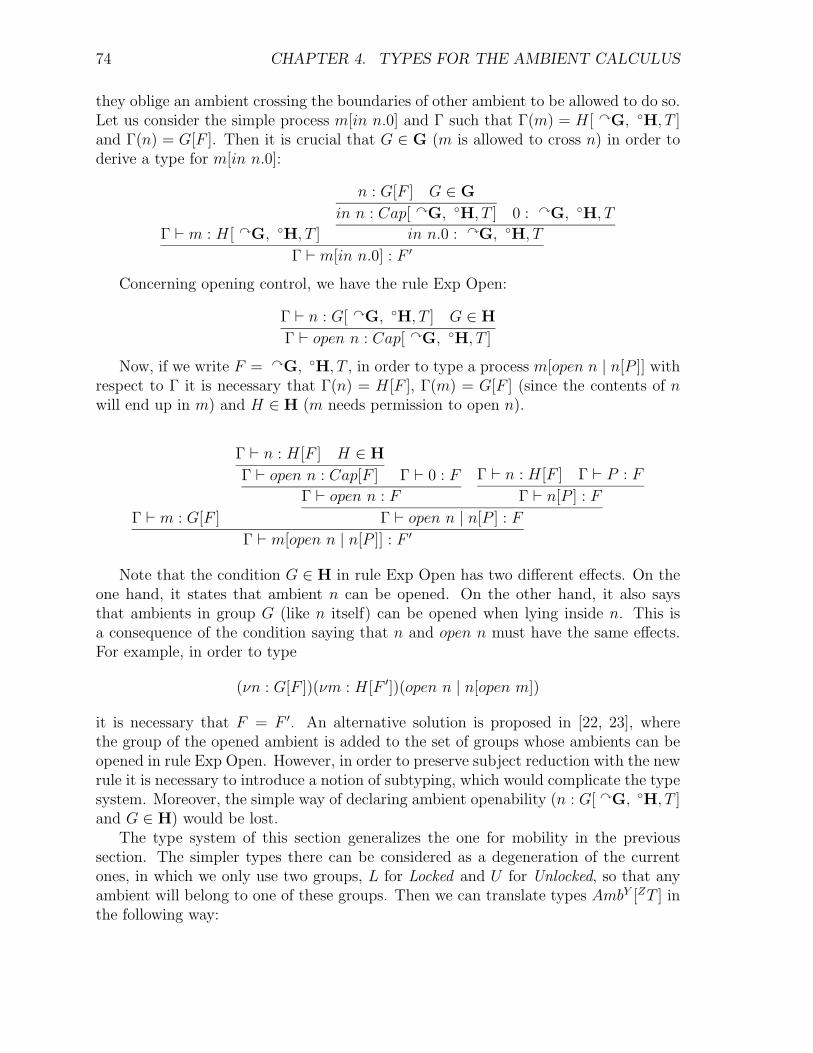
74 CHAPTER 4. TYPES FOR THE AMBIENT CALCULUS
they oblige an ambient crossing the boundaries of other ambient to be allowed to do so.Let us consider the simple process m[in n.0] and Γ such that Γ(m) = H[ yG, ◦H, T ]and Γ(n) = G[F ]. Then it is crucial that G ∈ G (m is allowed to cross n) in order toderive a type for m[in n.0]:
Γ ` m : H[ yG, ◦H, T ]
n : G[F ] G ∈ G
in n : Cap[ yG, ◦H, T ] 0 : yG, ◦H, T
in n.0 : yG, ◦H, T
Γ ` m[in n.0] : F ′
Concerning opening control, we have the rule Exp Open:
Γ ` n : G[ yG, ◦H, T ] G ∈ H
Γ ` open n : Cap[ yG, ◦H, T ]
Now, if we write F = yG, ◦H, T , in order to type a process m[open n | n[P ]] withrespect to Γ it is necessary that Γ(n) = H[F ], Γ(m) = G[F ] (since the contents of nwill end up in m) and H ∈ H (m needs permission to open n).
Γ ` m : G[F ]
Γ ` n : H[F ] H ∈ H
Γ ` open n : Cap[F ] Γ ` 0 : F
Γ ` open n : F
Γ ` n : H[F ] Γ ` P : F
Γ ` n[P ] : F
Γ ` open n | n[P ] : F
Γ ` m[open n | n[P ]] : F ′
Note that the condition G ∈ H in rule Exp Open has two different effects. On theone hand, it states that ambient n can be opened. On the other hand, it also saysthat ambients in group G (like n itself) can be opened when lying inside n. This isa consequence of the condition saying that n and open n must have the same effects.For example, in order to type
(νn : G[F ])(νm : H[F ′])(open n | n[open m])
it is necessary that F = F ′. An alternative solution is proposed in [22, 23], wherethe group of the opened ambient is added to the set of groups whose ambients can beopened in rule Exp Open. However, in order to preserve subject reduction with the newrule it is necessary to introduce a notion of subtyping, which would complicate the typesystem. Moreover, the simple way of declaring ambient openability (n : G[ yG, ◦H, T ]and G ∈ H) would be lost.
The type system of this section generalizes the one for mobility in the previoussection. The simpler types there can be considered as a degeneration of the currentones, in which we only use two groups, L for Locked and U for Unlocked, so that anyambient will belong to one of these groups. Then we can translate types AmbY [ZT ] inthe following way:

4.3. AMBIENT GROUPS 75
• tr(Amb•[yT ]) = L[y{L,U}, ◦{U}, T ]. It is a locked ambient that may cross anyambient, may open any unlocked ambient and contain T exchanges.
• tr(Amb•[YT ]) = L[y{}, ◦{U}, T ]. It is a locked ambient that cannot cross anyambient (it cannot move), may open any unlocked ambient and contain T ex-changes.
• tr(Amb◦[yT ]) = U [y{L,U}, ◦{U}, T ]. It is an unlocked ambient that may crossany ambient, may open any unlocked ambient and contain T exchanges.
• tr(Amb◦[YT ]) = U [y{}, ◦{U}, T ]. It is an unlocked ambient that cannot crossany ambient, may open any unlocked ambient and contain T exchanges.
Then, if we define tr(P ) and tr(Γ) as in the previous section it can be proven thatif Γ ` P : T holds in the previous type system then L,U, tr(Γ) ` tr(P ) : tr(T ) holds inthe current type system.
4.3.2 Access control runtime errors
Next we formalize run-time errors by means of aΓ→ err4 relation. Its definition, in
Figure 4.10, is quite similar to that ofΓ→ err3, except that now we control not only the
moving ambient or the opened ambient, but also the crossed ambient and the openerambient.
A safety theorem is proven in [26]. It regards the effect assigned to a process asan upper bound of the capabilities that the process may exercise, and hence on itsbehavior. We say that P exercises a capability M at its top level if P ↓ M can bederived from the rules in Figure 4.11.
Now, the safety theorem states that the set formed over groups of names containedin any capability that appears in a well-typed process is bounded by the effect assignedto the process.
Theorem 10 Assume that Γ ` P : yG, ◦H, T . Then,
1. If P ↓ in n then Γ ` n : G[F ] for some G[F ] with G ∈ G.
2. If P ↓ out n then Γ ` n : G[F ] for some G[F ] with G ∈ G.
3. If P ↓ open n then Γ ` n : G[F ] for some G[F ] with G ∈ H.
This theorem is a sufficient condition for the absence of run-time errors of typeerr4. For instance, let us suppose that Q is a well-typed process with respect to an
environment Γ, such that QΓ→ err4 can be obtained by applying the rule for In to
the subterm n[in m.P1 | P2] | m[R], which satisfies in m.P1 | P2 ↓ in m. Since Q iswell-typed so must be that subterm and, therefore, if Γ(n) = G[ yG, ◦H, T ], as a

76 CHAPTER 4. TYPES FOR THE AMBIENT CALCULUS
Γ(n) = G[ yG, ◦H, Shh]
n[(x1 : W1, . . . , xk : Wk)P | 〈M1, . . . ,Mk〉 | Q]Γ→ err4
Γ(n) = G[ yG, ◦H,W ′1 × . . . × W ′
r] k 6= r
n[(x1 : W1, . . . , xk : Wk)P | 〈M1, . . . ,Mk〉 | Q]Γ→ err4
Γ(n) = G[ yG, ◦H,W ′1 × . . . × W ′
k] ∃i.Wi 6= W ′i
n[(x1 : W1, . . . , xk : Wk)P | 〈M1, . . . ,Mk〉 | Q]Γ→ err4
Γ(n) = G[ yG, ◦H,W1 × . . . × Wk] ∃i.Γ 6` Mi : Wi
n[(x1 : W1, . . . , xk : Wk)P | 〈M1, . . . ,Mk〉 | Q]Γ→ err4
PΓ,n:W−→ err4
(νn : W )PΓ→ err4
P ≡ Q QΓ→ err4
PΓ→ err4
PΓ→ err4
P | QΓ→ err4
PΓ→ err4
n[P ]Γ→ err4
P → err1
PΓ→ err4
Γ(n) = G[ yG, ◦H, T ] Γ(m) = H[F ] H 6∈ G
n[in m.P | Q] | m[R]Γ→ err4
Γ(n) = G[ yG, ◦H, T ] Γ(m) = H[F ] H 6∈ G
m[n[out m.P | Q] | R]Γ→ err4
Γ(n) = G[ yG, ◦H, T ] Γ(m) = H[F ] H 6∈ H
n[open m.P | m[Q] | R]Γ→ err4
Figure 4.10: Rules for errors of fourth class
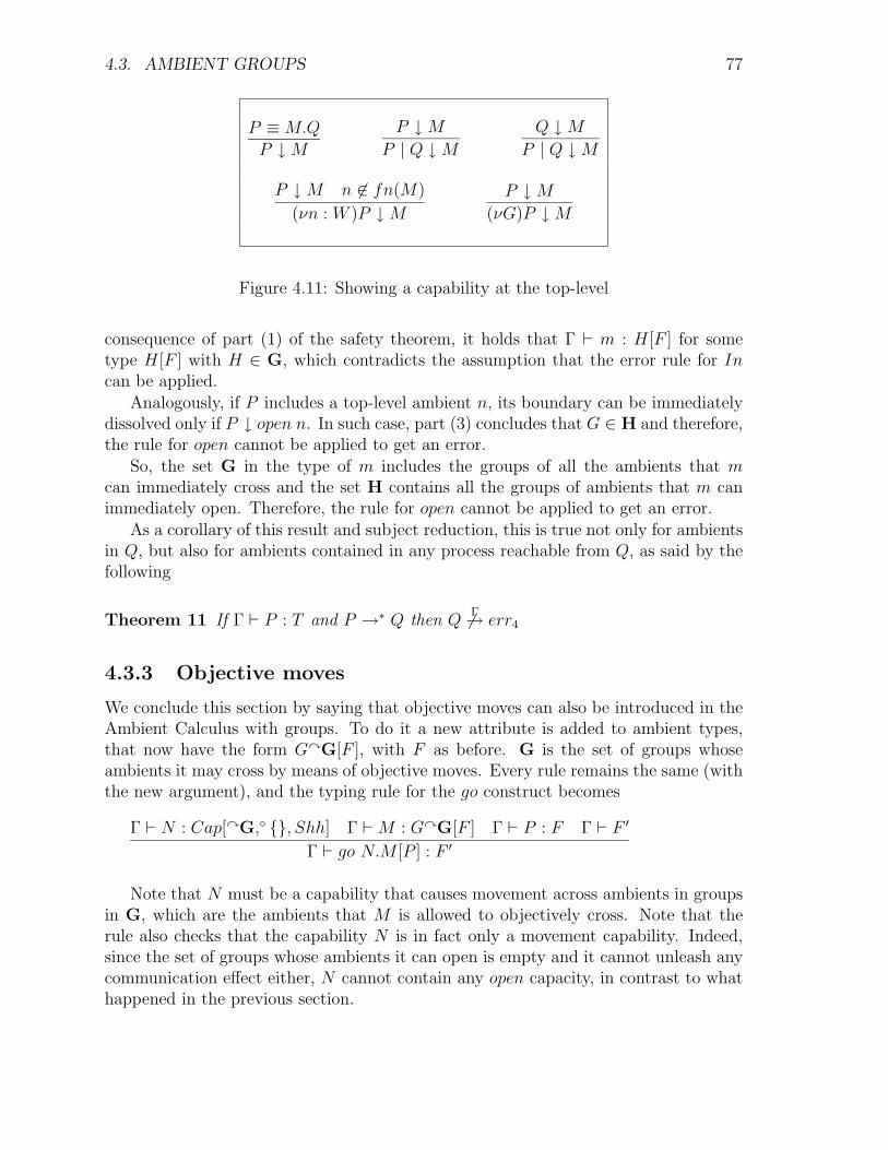
4.3. AMBIENT GROUPS 77
P ≡ M.Q
P ↓ M
P ↓ M
P | Q ↓ M
Q ↓ M
P | Q ↓ M
P ↓ M n 6∈ fn(M)
(νn : W )P ↓ M
P ↓ M
(νG)P ↓ M
Figure 4.11: Showing a capability at the top-level
consequence of part (1) of the safety theorem, it holds that Γ ` m : H[F ] for sometype H[F ] with H ∈ G, which contradicts the assumption that the error rule for Incan be applied.
Analogously, if P includes a top-level ambient n, its boundary can be immediatelydissolved only if P ↓ open n. In such case, part (3) concludes that G ∈ H and therefore,the rule for open cannot be applied to get an error.
So, the set G in the type of m includes the groups of all the ambients that mcan immediately cross and the set H contains all the groups of ambients that m canimmediately open. Therefore, the rule for open cannot be applied to get an error.
As a corollary of this result and subject reduction, this is true not only for ambientsin Q, but also for ambients contained in any process reachable from Q, as said by thefollowing
Theorem 11 If Γ ` P : T and P →∗ Q then Q 6Γ→ err4
4.3.3 Objective moves
We conclude this section by saying that objective moves can also be introduced in theAmbient Calculus with groups. To do it a new attribute is added to ambient types,that now have the form GyG[F ], with F as before. G is the set of groups whoseambients it may cross by means of objective moves. Every rule remains the same (withthe new argument), and the typing rule for the go construct becomes
Γ ` N : Cap[yG,◦ {}, Shh] Γ ` M : GyG[F ] Γ ` P : F Γ ` F ′
Γ ` go N.M [P ] : F ′
Note that N must be a capability that causes movement across ambients in groupsin G, which are the ambients that M is allowed to objectively cross. Note that therule also checks that the capability N is in fact only a movement capability. Indeed,since the set of groups whose ambients it can open is empty and it cannot unleash anycommunication effect either, N cannot contain any open capacity, in contrast to whathappened in the previous section.
78 CHAPTER 4. TYPES FOR THE AMBIENT CALCULUS
As for types, the old rules for err4 remain the same, except that now they arerelative to the new types. The new errors, caused by illicit objective moves, are:
Γ(n) = GyG[F ] Γ(m) = HyH[F ′] H 6∈ G
go(in m.N).n[P ] | m[R]Γ→ err4
Γ(n) = GyG[F ] Γ(m) = HyH[F ′] H 6∈ G
m[go(out m.N).n[P ] | Q]Γ→ err4
which state that any ambient objectively crossing another ambient must have thepermission to do it. The corresponding safety theorem with respect err4 also holdswhen adding objective moves.
4.4 Other type systems
The first extension of the original type system for the ambient calculus that introducessubtyping can be found in [74]. Subtyping forces us to unfold process types: insteadof ZT now they are ZO I, meaning that the corresponding processes can outputmessages of type O and input messages of type I. Subtyping, as usual, is covariant inoutputs and contravariant in inputs. Also, ambient types have two perspectives: whatmessages can be communicated inside (informative view) and what ambients can safelyopen them (restrictive view). This duality forces us again to unfold ambient types, thatnow become AmbY [T1, T2] (with T1 <: T2), contravariant on T1 and covariant in T2.A type-checking algorithm which returns a minimal type relative to this system ispresented in [74]. Also, a type-inference algorithm for the original type system withouttype annotations in the syntax is presented. As far as we know, those efforts to finda type-inference algorithm for the type system with subtyping have failed, because noalgorithmic method for solving the resulting set of constraints has been found.
In [7] several ways in which ambients can be said to be polymorphically typed arediscussed. Two of them, namely subtype polymorphism and orderly communication(that allows the type of exchanged data to vary over time) are considered in the typesystem presented there. Also a denotational semantics of types (trace semantics) isproposed and it is proved that type-checking is decidable. In [8] something similar isdone, although in a more reduced framework, without subtypes.
Finally, [50] presents a theory of dependant types for the Ambient Calculus, toexpress policies like n CanMoveTo m directly, without embodying groups in types.

Chapter 5
Extensions of the Ambient Calculus
Many different calculus have emerged as extensions of the Ambient Calculus, as result ofdifferent concerns and emphases of several groups of researchers. Almost all of them areequipped with a type system that controls certain aspects of importance. Nevertheless,in many cases only the intuitive meanings of these types are given and, at most, asubject reduction theorem is proven. We consider that a formal interpretation of thetype results (what properties are statically captured) is crucial in the development ofa type system. We will point out in the following some deficiencies that were found inthis respect.1
In the next sections a brief overview of several extensions or modifications of theAmbient Calculus will be presented, emphasizing whatever novelty in them, speciallyconcerning types. We will not give every single technical details, since they can befound in the original papers presenting each extension. We will only introduce thosenecessary details for the understanding of the main underlying ideas. Figure 5.1 is adiagram of the dependency relations among these extensions.
5.1 Safe Ambients
The Safe Ambients (SA) Calculus appears as a consequence of the study of interfer-ences in AC, more precisely those interferences that arise from the redex election. InCardelli’s Calculus plain interferences can occur (as in CCS or π-calculus), when aprocess can interact using the same capability with two different partners (these cor-respond to the situation of two processes competing for the same resource). Processes(5.1) and (5.2) are examples of this situation.
n[in m.P ] | m[Q] | m[R] (5.1)
open n.P | open n.Q | n[R] (5.2)
1After all, a particular type system in which subject reduction holds is that in which every termis well typed having the same type
79
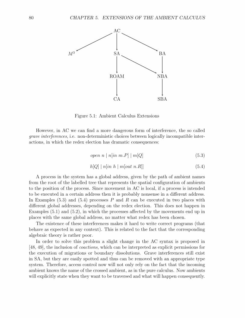
80 CHAPTER 5. EXTENSIONS OF THE AMBIENT CALCULUS
AC
M3 SA BA
ROAM
CA
NBA
SBA
Figure 5.1: Ambient Calculus Extensions
However, in AC we can find a more dangerous form of interference, the so calledgrave interferences, i.e. non-deterministic choices between logically incompatible inter-actions, in which the redex election has dramatic consequences:
open n | n[in m.P ] | m[Q] (5.3)
h[Q] | n[in h | m[out n.R]] (5.4)
A process in the system has a global address, given by the path of ambient namesfrom the root of the labelled tree that represents the spatial configuration of ambientsto the position of the process. Since movement in AC is local, if a process is intendedto be executed in a certain address then it is probably nonsense in a different address.In Examples (5.3) and (5.4) processes P and R can be executed in two places withdifferent global addresses, depending on the redex election. This does not happen inExamples (5.1) and (5.2), in which the processes affected by the movements end up inplaces with the same global address, no matter what redex has been chosen.
The existence of these interferences makes it hard to write correct programs (thatbehave as expected in any context). This is related to the fact that the correspondingalgebraic theory is rather poor.
In order to solve this problem a slight change in the AC syntax is proposed in[48, 49], the inclusion of coactions, which can be interpreted as explicit permissions forthe execution of migrations or boundary dissolutions. Grave interferences still existin SA, but they are easily spotted and thus can be removed with an appropriate typesystem. Therefore, access control now will not only rely on the fact that the incomingambient knows the name of the crossed ambient, as in the pure calculus. Now ambientswill explicitly state when they want to be traversed and what will happen consequently.

5.1. SAFE AMBIENTS 81
5.1.1 Syntax and semantics
Concerning the syntax, the main change is at the level of expressions, where the fol-lowing new capacities are added:
M,N := . . . | in M | out M | open M
With respect to processes, the only novelty is the substitution of the replicationconstruct !P by the recursion construct rec X.P , where the process variable X cannotappear within ambients in P . Therefore typing environments will also have processvariables in their domain. This change simplifies the type system.
The axioms for mobility are the following:
n[in m.P1 | P2] | m[in m.Q1 | Q2] → m[n[P1 | P2] | Q1 | Q2]m[n[out m.P1 | P2] | out m.Q1 | Q2] → n[P1 | P2] | m[Q1 | Q2]
open n.P | n[open n.Q1 | Q2] → P | Q1 | Q2
Unlike the original calculus, it does not suffice knowing the name of an ambient tocross or dissolve its boundaries. Moreover, as the ambient that receives the action isaware of it, it can respond properly.
5.1.2 Types
In [48] three type systems, that can be combined one another, are developed: oneof basic types (analogous to Cardelli and Gordon’s types for communication control[26]), one for immobile ambients (which cannot move or be opened) and another one forsingle threaded (ST) ambients (in which there is at most one active sequential process).The type system for immobile ambients is similar to the basic one, except that it doesnot assign types to processes that may perform movements. The proper combinationof basic and immobility types gives us a type system similar to the type system formobility control in Chapter 4 (except that immobile ambients are exactly those thatcannot be opened). Rules for recursive processes, restriction, variables, names and thenil process are common for the three type system. Now let us focus on the descriptionof the ST types.
Usually, the control within an ambient is distributed over its local processes, thatis, any of its sequential components can exercise a capability. However, within a STambient at most one process has the thread and can, therefore, execute an action.
The thread can move from one ST process to another by means of an open action.Let us consider the next reduction, where n and m are ST ambients:
n[open m.P | m[open m.Q]] → n[P | Q]
At the beginning the process open m.P has the control over n and open m.Q hasit over m. But, what process is allowed to execute an action after the reduction, P orQ? The type system will consider these situations and will explicitly say which processwill continue the execution.
A similar problem arises in the reading of messages. Let us consider the process

82 CHAPTER 5. EXTENSIONS OF THE AMBIENT CALCULUS
Thread rights Message types
I,J:=↑ (thread) Tt:=IW (ST messages)| † (no thread) | Shh (no messages)
Expression Types Process Types
Amb:=STAmbI[Tt] (ST Ambient) Proc:=STProcI[Tt] (ST Process)Cap:=STCapI[Tt] (ST Capacity)
Figure 5.2: ST Types
n[in h.〈m〉 | (x).in x.Q] | h[in h.R] → → h[R | n[in m.Q]]
At first, in h.〈m〉 has the thread in n but the consumption of 〈m〉 makes in x.Qhave the thread. On the other hand, in process
n[(x).m[x.P ] | 〈in h〉 | in n] | h[in n.in m]
within n the subprocess in n has the thread independently of the consumption of themessage. Therefore, the ST types will have to control whether message consumptioninterferes with control or not.
ST types, defined in Figure 5.2 have the following intuitive meanings:
- STAmbI[Tt] is the type of ambients that contain at most one sequential processwith thread. When opened it keeps the thread if I =↑ or it yields it to the processthat opened it if I = †. In addition, messages of type Tt are exchanged inside.
- STCapI[Tt] is the type of the capacities that can precede a ST process and canrelease Tt messages. It will grant the thread to its remainder (the process itprefixes) if I =↑ and it will not if I = †.
- STProcI[Tt] is the type of processes local to an ST ambient that can releasemessages of type Tt and that are active if I =↑ or inactive if I = †.
- IW is the type of messages of type W . If I =↑ then message consumption meansacquiring the thread. If I = † then control is independent of communication.
Let us comment on the most important rules of the type system in Figure 5.3. InST-open ↑−1= † and viceversa. If M : STAmb ↑ [Tt] then M is an ambient that keepsthe thread when opened and, therefore, open M does not give it to its continuation(dually if I = †). Rule ST-inout says that an ST-ambient can enter any ambient (Amb

5.1. SAFE AMBIENTS 83
stands for any ambient type: basic, immobile or ST). On the contrary, cocapabilitiesin N and out N are supposed to be used inside ambient N and, therefore, rule ST-coinout states that if N is ST so has to be the capacity.
Regarding processes, according to rule ST-pref, prefixed processes always have thethread and the continuation may have it only if its prefix gives does not give it away.Rules ST-par1 (and the corresponding ST-par2) and ST-par† for parallel compositionsay that in order to type as ST a process with two parallel components, at least one ofthem has to be dead and the result is dead only if both components are. The remainingfour rules can be better understood if we consider that, so far, the type system hasan implicit notion of subtyping by which if a process can be typed as STProc†[Tt]then it can also be typed as STProc ↑ [Tt] (it is more difficult to type with †). Thissubtyping will be needed to preserve the type of a process along its computation.Thus, in the following, if the conclusion of a rule states that a process can be typedwith an arbitrary thread right J it means that it can be typed with J = † but, tomaintain that notion of subtyping it can also be typed as J =↑. Rules ST-msg1 andST-msg2 state that a message does not have the thread only if message consumptionis independent of control. In principle, input processes do not have the thread. Ifmessage consumption does not mean acquiring the thread then its continuation mustbe typed without thread. Rule ST-rec is just an implicit subsumption rule for recursiveprocesses.
In addition, we have rules that combine the two basic type systems with the onehere presented. We focus on those that allow interaction between immobile and singlethreaded ambients. If n is an ambient that looses its thread when opened, and itsprocesses cannot acquire it by message consumption then it is possible to open it whenlying on an immobile ambient, since the fact that it has no thread implies that it doesnot have any movement capabilities. Two additional rules are added:
(ST-I-open1) (ST-I-open2)
Γ ` M : STAmb†[†W ]
Γ ` open M : ICap[W ]
Γ ` M : STAmb†[Shh]
Γ ` open M : ICap[Shh]
Consider the next illustrative example:
Q = n[in n | open h | (x : W )P ] | h[in n.open h.〈M〉]]
Let us suppose that Γ(h) = STAmb†[†W ], Γ(n) = IAmb[W ], Γ ` M : W andΓ, x : W ` P : IProc[W ]. That means that n, an immobile ambient, intends to openh, even though it is mobile. Note that h is an ambient that looses its thread whenopened, nor can it acquire it by means of message consumption. It can be verifiedthat Q is perfectly typeable in the type system described, under the above restrictions.This partially overcomes the problem we had in Chapter 4.

84 CHAPTER 5. EXTENSIONS OF THE AMBIENT CALCULUS
Expression Types
M ∈ {in N, out N} Γ ` N : Amb
Γ ` M : STCap ↑ [Tt] ST-inout
M ∈ {in N, out N} Γ ` N : STAmbI[Tt]
Γ ` M : STCap ↑ [Tt′] ST-coinout
Γ ` M : STAmbI[Tt]
Γ ` open M : STCapI−1[Tt] ST-open
Γ ` M : STAmbI[Tt]
Γ ` open M : StCapI[Tt] ST-coopen
Process Types
Γ ` M : STCapI[Tt] Γ ` P : STProcI[Tt]
Γ ` M.P : StProc ↑ [Tt] ST-pref
Γ ` P1 : STProc ↑ [Tt] Γ ` P2 : STProc†[Tt]
Γ ` P1 | P2 : STProc ↑ [Tt] ST-par1
Γ ` P1 : STProc†[Tt] Γ ` P2 : STProc†[Tt]
Γ ` P1 | P2 : STProc†[Tt] ST-par†
Γ, x : W ` P : STProcI[IW ]
Γ ` (x : W )P : STProcJ [IW ] ST-abs
Γ ` M : WΓ ` 〈M〉 : STProc ↑ [↑ W ] ST-msg1
Γ ` M : WΓ ` 〈M〉 : STProcJ [†W ] ST-msg1
Γ ` rec X.P : STProc†[Tt]
Γ ` rec X.P : STProc ↑ [Tt] ST-rec
Figure 5.3: Typing rules for ST types

5.1. SAFE AMBIENTS 85
5.1.3 Main results on typed processes
The three type systems defined in [48] and their combination satisfy the correspondingsubject reduction theorems. Also, processes of type ST are indeed single threaded, asstated in the following theorem:
Theorem 12
1. If Γ ` P : STProc†[Tt] then P has no unguarded capabilities; moreover ifTt =↑ W then P has also no unguarded messages.
2. If Γ ` P : STProc ↑ [Tt] then P has at most one unguarded capability; moreoverif Tt =↑ W then P has at most one unguarded capability or message.
Both ST types and immobility types can be used to rule out grave interferences fromSafe Ambients. As the presence of such grave interferences can be statically spottedthe following theorem is proven:
Theorem 13 If P is closed and the type of each name defined in Γ and each restrictedname in P is immobile or ST then P has no grave interferences.
As a corollary of this theorem and subject reduction we have the one stated in [48]
Theorem 14 Let us suppose that Γ ` P : Proc where P is closed. Assuming that thetype of each name defined in Γ and each restricted name in P is immobile or ST, thenfor all P ′ such that P →∗ P ′, process P ′ has no grave interferences.
The formalization of interferences within SA (which will not be discussed here)takes profit of the fact that in the presence of coactions grave interferences are exactlythose in which the two simultaneous redexes that cause the interference do not overlap.
5.1.4 Renaming as an example
Let us consider the construction proposed in [25] for introducing ambient renaming:
n be m.P4= m[out n.open n.P ] | in m
The process n be m.P inside an ambient called n can change its name to m, that is,
n[n be m.P | Q] →∗ m[P | Q]
However, there are many ways in which the context or Q itself can interfere with thecorrect execution of the protocol (the context could contain ambients named n or m,or ambients that tried to enter n or open n or m; Q could contain processes that movedn or ambients that exited from n).
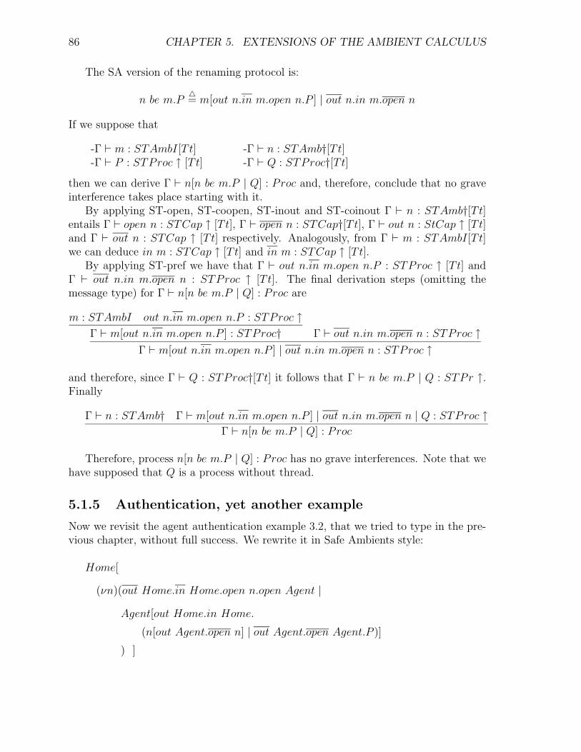
86 CHAPTER 5. EXTENSIONS OF THE AMBIENT CALCULUS
The SA version of the renaming protocol is:
n be m.P4= m[out n.in m.open n.P ] | out n.in m.open n
If we suppose that
-Γ ` m : STAmbI[Tt] -Γ ` n : STAmb†[Tt]-Γ ` P : STProc ↑ [Tt] -Γ ` Q : STProc†[Tt]
then we can derive Γ ` n[n be m.P | Q] : Proc and, therefore, conclude that no graveinterference takes place starting with it.
By applying ST-open, ST-coopen, ST-inout and ST-coinout Γ ` n : STAmb†[Tt]entails Γ ` open n : STCap ↑ [Tt], Γ ` open n : STCap†[Tt], Γ ` out n : StCap ↑ [Tt]and Γ ` out n : STCap ↑ [Tt] respectively. Analogously, from Γ ` m : STAmbI[Tt]we can deduce in m : STCap ↑ [Tt] and in m : STCap ↑ [Tt].
By applying ST-pref we have that Γ ` out n.in m.open n.P : STProc ↑ [Tt] andΓ ` out n.in m.open n : STProc ↑ [Tt]. The final derivation steps (omitting themessage type) for Γ ` n[n be m.P | Q] : Proc are
m : STAmbI out n.in m.open n.P : STProc ↑
Γ ` m[out n.in m.open n.P ] : STProc† Γ ` out n.in m.open n : STProc ↑
Γ ` m[out n.in m.open n.P ] | out n.in m.open n : STProc ↑
and therefore, since Γ ` Q : STProc†[Tt] it follows that Γ ` n be m.P | Q : STPr ↑.Finally
Γ ` n : STAmb† Γ ` m[out n.in m.open n.P ] | out n.in m.open n | Q : STProc ↑
Γ ` n[n be m.P | Q] : Proc
Therefore, process n[n be m.P | Q] : Proc has no grave interferences. Note that wehave supposed that Q is a process without thread.
5.1.5 Authentication, yet another example
Now we revisit the agent authentication example 3.2, that we tried to type in the pre-vious chapter, without full success. We rewrite it in Safe Ambients style:
Home[
(νn)(out Home.in Home.open n.open Agent |
Agent[out Home.in Home.
(n[out Agent.open n] | out Agent.open Agent.P )]
) ]

5.1. SAFE AMBIENTS 87
A slight change has been made with respect to the original protocol, that does notaffect its behavior. Now it is ambient Home that exercises the open Agent capability,instead of n. However, the authentication has already been fulfilled (at an intuitivelevel), since that capability is only exercised after the opening of n. The process canevolve in the following way, analogously to the original one (omitting the restrictionoperator for the sake of readability):
Home[out Home.in Home.open n.open Agent |
Agent[out Home.in Home.(n[out Agent.open n] | out Agentopen Agent.P )]]
→ Home[in Home.open n.open Agent] |
Agent[in Home.(n[out Agent.open n] | out Agent.open Agent.P )]
→ Home[open n.open Agent |
Agent[n[out Agent.open n] | out Agent.open Agent.P ]]
→ Home[open n.open Agent | n[open n] | Agent[open Agent.P ]]
→ Home[open Agent | Agent[open Agent.P ]]
→ Home[P ]
Let us type this process under the restriction that Home is an immobile ambient.Within Home mobile ambients are opened, Agent and n, and therefore we have totype the content of those ambients as single threaded processes that loose the threadwhen opened. Therefore we assume that
Γ(Home) = IAmb[T ] Γ(Agent) = STAmb†[Tt]
Γ(n) = STAmb†[Tt] Γ ` P : STProc†[Tt]
where Tt = Shh if T = Shh or Tt = †W if T = W .We write the process with the following notations:
Home[M | Agent[N1.(n[N2] | Q)]]
where we abbreviate M = out Home.in Home.open n.open Agent, N1 = out Home.in Home,N2 = out Agent.open n and Q = out Agent.open Agent.P . We have the followingderivations (as always, we omit the communication attribute):
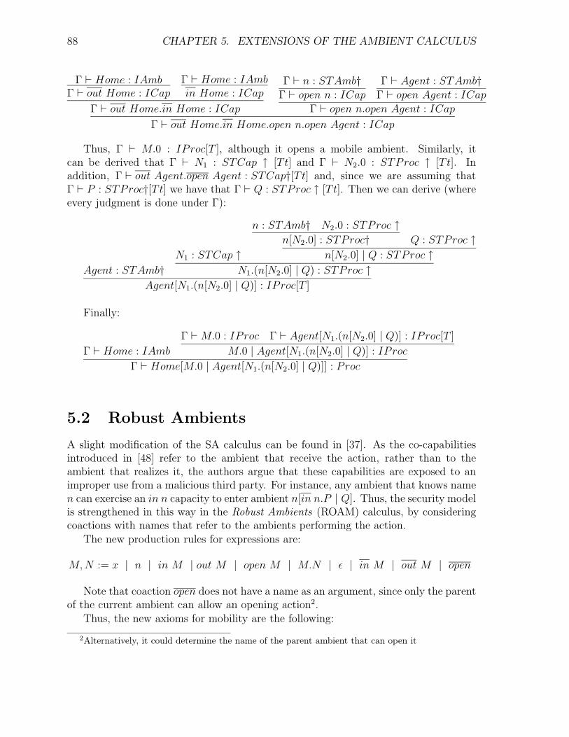
88 CHAPTER 5. EXTENSIONS OF THE AMBIENT CALCULUS
Γ ` Home : IAmbΓ ` out Home : ICap
Γ ` Home : IAmbin Home : ICap
Γ ` out Home.in Home : ICap
Γ ` n : STAmb†Γ ` open n : ICap
Γ ` Agent : STAmb†Γ ` open Agent : ICap
Γ ` open n.open Agent : ICap
Γ ` out Home.in Home.open n.open Agent : ICap
Thus, Γ ` M.0 : IProc[T ], although it opens a mobile ambient. Similarly, itcan be derived that Γ ` N1 : STCap ↑ [Tt] and Γ ` N2.0 : STProc ↑ [Tt]. Inaddition, Γ ` out Agent.open Agent : STCap†[Tt] and, since we are assuming thatΓ ` P : STProc†[Tt] we have that Γ ` Q : STProc ↑ [Tt]. Then we can derive (whereevery judgment is done under Γ):
Agent : STAmb†
N1 : STCap ↑
n : STAmb† N2.0 : STProc ↑
n[N2.0] : STProc† Q : STProc ↑
n[N2.0] | Q : STProc ↑
N1.(n[N2.0] | Q) : STProc ↑
Agent[N1.(n[N2.0] | Q)] : IProc[T ]
Finally:
Γ ` Home : IAmb
Γ ` M.0 : IProc Γ ` Agent[N1.(n[N2.0] | Q)] : IProc[T ]
M.0 | Agent[N1.(n[N2.0] | Q)] : IProc
Γ ` Home[M.0 | Agent[N1.(n[N2.0] | Q)]] : Proc
5.2 Robust Ambients
A slight modification of the SA calculus can be found in [37]. As the co-capabilitiesintroduced in [48] refer to the ambient that receive the action, rather than to theambient that realizes it, the authors argue that these capabilities are exposed to animproper use from a malicious third party. For instance, any ambient that knows namen can exercise an in n capacity to enter ambient n[in n.P | Q]. Thus, the security modelis strengthened in this way in the Robust Ambients (ROAM) calculus, by consideringcoactions with names that refer to the ambients performing the action.
The new production rules for expressions are:
M,N := x | n | in M | out M | open M | M.N | ε | in M | out M | open
Note that coaction open does not have a name as an argument, since only the parentof the current ambient can allow an opening action2.
Thus, the new axioms for mobility are the following:
2Alternatively, it could determine the name of the parent ambient that can open it
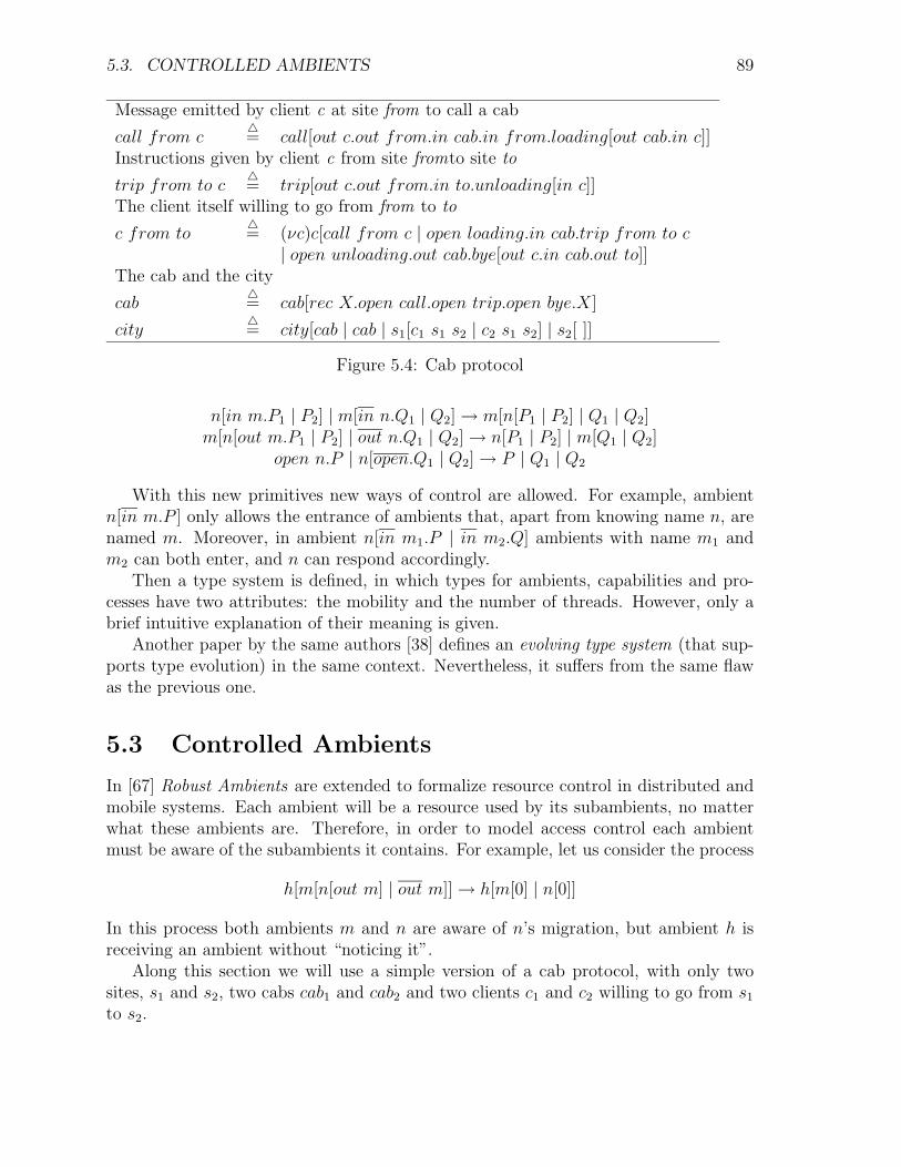
5.3. CONTROLLED AMBIENTS 89
Message emitted by client c at site from to call a cab
call from c4= call[out c.out from.in cab.in from.loading[out cab.in c]]
Instructions given by client c from site fromto site to
trip from to c4= trip[out c.out from.in to.unloading[in c]]
The client itself willing to go from from to to
c from to4= (νc)c[call from c | open loading.in cab.trip from to c
| open unloading.out cab.bye[out c.in cab.out to]]The cab and the city
cab4= cab[rec X.open call.open trip.open bye.X]
city4= city[cab | cab | s1[c1 s1 s2 | c2 s1 s2] | s2[ ]]
Figure 5.4: Cab protocol
n[in m.P1 | P2] | m[in n.Q1 | Q2] → m[n[P1 | P2] | Q1 | Q2]m[n[out m.P1 | P2] | out n.Q1 | Q2] → n[P1 | P2] | m[Q1 | Q2]
open n.P | n[open.Q1 | Q2] → P | Q1 | Q2
With this new primitives new ways of control are allowed. For example, ambientn[in m.P ] only allows the entrance of ambients that, apart from knowing name n, arenamed m. Moreover, in ambient n[in m1.P | in m2.Q] ambients with name m1 andm2 can both enter, and n can respond accordingly.
Then a type system is defined, in which types for ambients, capabilities and pro-cesses have two attributes: the mobility and the number of threads. However, only abrief intuitive explanation of their meaning is given.
Another paper by the same authors [38] defines an evolving type system (that sup-ports type evolution) in the same context. Nevertheless, it suffers from the same flawas the previous one.
5.3 Controlled Ambients
In [67] Robust Ambients are extended to formalize resource control in distributed andmobile systems. Each ambient will be a resource used by its subambients, no matterwhat these ambients are. Therefore, in order to model access control each ambientmust be aware of the subambients it contains. For example, let us consider the process
h[m[n[out m] | out m]] → h[m[0] | n[0]]
In this process both ambients m and n are aware of n’s migration, but ambient h isreceiving an ambient without “noticing it”.
Along this section we will use a simple version of a cab protocol, with only twosites, s1 and s2, two cabs cab1 and cab2 and two clients c1 and c2 willing to go from s1
to s2.

90 CHAPTER 5. EXTENSIONS OF THE AMBIENT CALCULUS
In Figure 5.4 the city is an ambient, which contains cabs and sites, represented alsoas ambients. Sites can contain client ambients. Ambient call will be sent from theclient to any taxi. Several other synchronization ambients, such as loading, unloadingor bye are also used. In this example, the system will be resource-controlled if at anytime each cab contains at most one client.
It can be checked that, in a correct execution of the protocol, both clients end up ins2, whether using both cabs concurrently or the same cab one after the other. However,there are various flaws in the protocol. If we consider the following computation
city →∗
city[s1[c1[in cab. . . .] | c2[in cab. . . .] | cab[. . .] | cab[. . .]]]
we reach a point where the clients can non deterministically choose which cab to enterand, in particular, they can choose the same cab. A version of the protocol in the newcalculus will solve this problem.
In [67] an alternative of coactions is proposed, as a further development of [37], tosolve these problems.
5.3.1 Syntax and semantics
In the language of Controlled Ambients (CA) every movement is constrained by a3-way synchronization between the ambient moving, the ambient welcoming the movingambient and the ambient allowing it to exit. This synchronization is handled by meansof the following coactions:
· in↑ m welcomes ambient m coming from a subambient.
· in↓ m welcomes ambient m coming from the parent ambient.
· out↑ m allows ambient m to exit to the parent ambient.
· out↓ m allows ambient m to enter a subambient.
· open{m,h} allows ambient h to open ambient m.
The new reduction axioms for Controlled Ambients are:
m[in n.P | Q] | n[in↓ m.R | S] | out↓ m.T → n[m[P | Q] | R | S] | T
n[m[out n.P | Q] | out↑m.R] | S] | in↑ m.T → m[P | Q] | n[R | S] | T
h[open m.P | Q | m[open{m,h}.R | S]] → h[P | Q | R | S]
recX.P → P{X := recX.P}
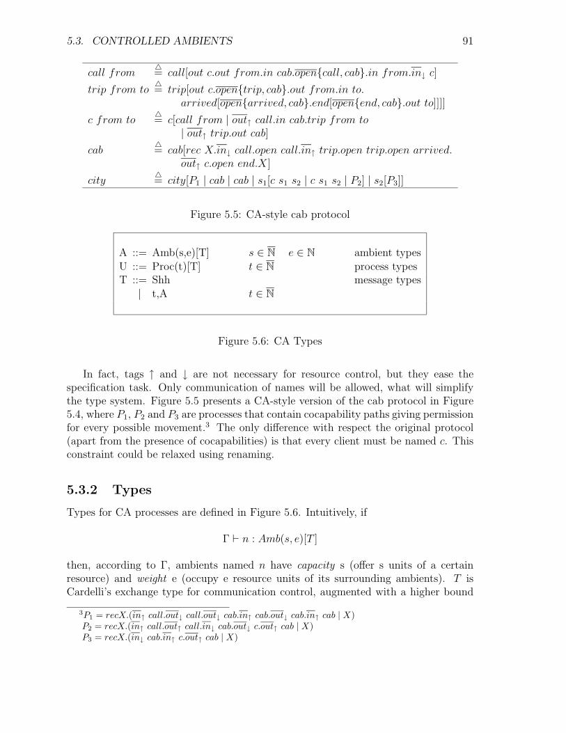
5.3. CONTROLLED AMBIENTS 91
call from4= call[out c.out from.in cab.open{call, cab}.in from.in↓ c]
trip from to4= trip[out c.open{trip, cab}.out from.in to.
arrived[open{arrived, cab}.end[open{end, cab}.out to]]]]
c from to4= c[call from | out↑ call.in cab.trip from to
| out↑ trip.out cab]
cab4= cab[rec X.in↓ call.open call.in↑ trip.open trip.open arrived.
out↑ c.open end.X]
city4= city[P1 | cab | cab | s1[c s1 s2 | c s1 s2 | P2] | s2[P3]]
Figure 5.5: CA-style cab protocol
A ::= Amb(s,e)[T] s ∈ N e ∈ N ambient types
U ::= Proc(t)[T] t ∈ N process typesT ::= Shh message types
| t,A t ∈ N
Figure 5.6: CA Types
In fact, tags ↑ and ↓ are not necessary for resource control, but they ease thespecification task. Only communication of names will be allowed, what will simplifythe type system. Figure 5.5 presents a CA-style version of the cab protocol in Figure5.4, where P1, P2 and P3 are processes that contain cocapability paths giving permissionfor every possible movement.3 The only difference with respect the original protocol(apart from the presence of cocapabilities) is that every client must be named c. Thisconstraint could be relaxed using renaming.
5.3.2 Types
Types for CA processes are defined in Figure 5.6. Intuitively, if
Γ ` n : Amb(s, e)[T ]
then, according to Γ, ambients named n have capacity s (offer s units of a certainresource) and weight e (occupy e resource units of its surrounding ambients). T isCardelli’s exchange type for communication control, augmented with a higher bound
3P1 = recX.(in↑ call.out↓ call.out↓ cab.in↑ cab.out↓ cab.in↑ cab | X)P2 = recX.(in↑ call.out↑ call.in↓ cab.out↓ c.out↑ cab | X)P3 = recX.(in↓ cab.in↑ c.out↑ cab | X)

92 CHAPTER 5. EXTENSIONS OF THE AMBIENT CALCULUS
on the effect of exchanging messages within n. Concerning processes, if
Γ ` P : Proc(t)[T ]
then P is a process that can use up to t resources and exchange messages of type T .The typing rules are in Figure 5.7. A subtyping theorem can be proved, stating
that if a process can be typed with weight t then it can also be typed with any weightt′ ≥ t. This theorem tells us that the side conditions in rules CA-coout and CA-opencan always be satisfied. Also, if a process is typeable under Γ with exchange type Tthen there is a minimal t such that Γ ` P : Proc(t)[T ]. There are three reasons why aprocess can have a positive weight:
1. It is an ambient, in which case its weight is specified by its name (CA-amb).
2. It is a parallel composition of two process and at least one of them has a positiveweight (CA-par).
3. It is a prefixed process and one of the prefixes is inδ m or open m. In this casethe typing rules load the capacities with the hypothetical weight they unleash(the weight of m in the former case and the maximum possible content of m inthe latter).
Let us take a closer view at the consequences of performing an opening. Let usconsider the process
m[open n | n[open{n,m}.Q]] → m[Q]
and suppose Γ ` n : Amb(sn, en)[Shh] and Γ ` m : Amb(sm, em)[Shh]. In order totype open n.0 we have to type Γ ` 0 : Proc(t)[Shh] in such a way that t− en + sn ≥ 0.Let us distinguish the two following cases:
1. en ≤ sn In this case that condition can be satisfied if we take t = 0 and we getΓ ` open n : Proc(sn − en)[Shh]. Since Γ ` n[open{n,m}.Q] : Proc(en)[Shh],by applying rule CA-par, Γ ` open n | n[open{n,m}.Q] : Proc(sn)[Shh].
2. en ≥ sn Then we can take t = en − sn and then we have Γ ` open n :Proc(0)[Shh]. By applying rule CA-par we get Γ ` open n | n[open{n,m}.Q] :Proc(en)[Shh]
In both cases we have obtained open n | n[open{n,m}.Q] : Proc(max{en, sn})[Shh],that is, we are taking as weight inside m along that computation step the maximumbetween the weight of n and the capacity of n (which, in turns, approximates thepossible weight inside n).
Something similar occurs with the outδ coaction. Here we take as the weight of theprocess n[m[out n.P ] | out↑ m.Q] the maximum between the weights of m and Q.

5.3. CONTROLLED AMBIENTS 93
Γ, X : Proc(t)[T ] ` P : Proc(t)[T ] t′ ≥ t
Γ ` rec X.P : Proc(t′)[T ] CA-rec
M ∈ {in m, out m, open{m,h}} Γ ` P : Proc(t)[T ]
Γ ` M.P : Proc(t)[T ] CA-pref1
Γ ` P : Proc(t)[T ] Γ ` m : Amb(s, e)[T ′]
Γ ` inδ m.P : Proc(t + e)[T ] CA-coin
Γ ` P : Proc(t)[T ] Γ ` m : Amb(s, e)[T ′] e ≤ t
Γ ` outδm.P : Proc(t − e)[T ] CA-coout
Γ ` P : Proc(t)[T ] Γ ` m : Amb(s, e)[T ] t − e + s ≥ 0
Γ ` open m.P : Proc(t − e + s)[T ] CA-open
Γ ` m : Amb(s, e)[T ] Γ ` P : Proc(a)[T ] a ≤ s
Γ ` m[P ] : Proc(e)[T ′] CA-amb
Γ ` P : Proc(t)[T ] Γ ` Q : Proc(t′)[T ]
Γ ` P | Q : Proc(t + t′)[T ] CA-par
Γ ` m : A t′ ≥ t
Γ ` 〈m〉 : Proc(t′)[t, A] CA-msg
Γ, x : A ` P : Proc(t)[t, A]
Γ ` (x : A)P : Proc(t′)[t, A] CA-rcv
Figure 5.7: Typing rules for CA types

94 CHAPTER 5. EXTENSIONS OF THE AMBIENT CALCULUS
5.3.3 Main results on typed processes
As we have said, a subtyping and a minimal type theorems are proven in [67]. Also,several properties captured by the type system are given. A resource policy compliancerelation |= is defined, so that Γ |= P holds if the total weight of the contents ofany ambient in P do not exceed its capacity, according to the weights and capacitiesspecified in Γ. Then the following theorems are proven:
Theorem 15 For any processes P,Q, resource policy Γ and type U , if Γ ` P : U andP → Q then Γ ` Q : U .
Theorem 16 For any process P , resource policy Γ and process type U , if Γ ` P : Uthen Γ |= P .
As a direct consequence we have the following main result:
Theorem 17 Under any resource policy Γ, if P is a process such that Γ ` P : U forsome U , then for any Q such that P →∗ Q, it holds that Γ |= Q.
5.3.4 Exclusive simultaneous access: a simple example
Let us consider the following resource policy:
Γ(c) = Amb(0, 1)[Ssh] Γ(end) = Amb(0, 0)[Ssh]Γ(call) = Amb(1, 0)[Ssh] Γ(cab) = Amb(1, 0)[Ssh]Γ(trip) = Amb(0, 0)[Ssh] Γ(si) = Amb(∞, 0)[Ssh]Γ(arrived) = Amb(0, 0)[Ssh] Γ(city) = Amb(0, 0)[Ssh]
We can see that it only restricts the number of clients that are simultaneously ata cab. Ambient call must be typed with capacity 1 because it is responsible for theentering of a client. Sites have infinite capacity, that is, there can be any number ofclients in sites. In order to simplify the corresponding type derivation we will writeP : t for Γ ` P : Proc(t)[Ssh] and n : (s, e) for Γ ` n : Amb(s, e)[Ssh]. Then we have:
c : (0, 1)
out c.out s1. . . . in↓ c : 1 call : (1, 0) 1 ≤ 1
call s1 : 0
In addition, trip s1 s2 : 0, what can be easily checked as none of the ambients thatappear in it has a positive weight, except for c, which appears as part of an out capacity.
Then we can derive

5.4. BOXED AMBIENTS 95
c : (0, 1)
call s1 : 0
call : (0, 0) in cab.trip s1 s2 : 0
out↑ call.in cab.trip s1 s2 : 0
trip : (0, 0) out cab : 0
out↑ trip.out cab : 0
call s1 | out↑ call.in cab.trip s1 s2 | out↑ trip.out cab : 0 0 ≤ 0
c s1 s2 : 1
Therefore c s1 s2 | c s1 s2 : 2 and since sites have infinite capacity, it can be derivedthat s1[c s1 s2 | c s1 s2 | P2] : 0 and s2[P3] : 0.
Now, since cab has capacity 1 we need to type its contents with weight at most 1.In the next judgments every time the variable X is not bounded we will suppose it isin the environment with weight 1 (if we assigned weight 0 to X then the process couldnot be typed).
call : (0, 0)
call(1, 0)
trip : (0, 0)
arrived : (0, 0)
c : (0, 1)
end : (0, 0) X : 1
open end.X : 1
out↑ c.open end.X : 0
open arrived.out↑ c.open end.X : 0
in↑ trip.open trip.open arrived.out↑ c.open end.X : 0
open call.in↑ trip.open trip.open arrived.out↑ c.open end.X : 1
in↓ call.open call.in↑ trip.open trip.open arrived.out↑ c.open end.X : 1
rec X.in↓ call.open call.in↑ trip.open trip.open arrived.out↑ c.open end.X : 1
Therefore we have cab : 0. The key point lies in the fact that the opening of callambient, that contains the in↓ c capacity, is counterbalanced by the out↑ c capacity.
Now we can conclude that Γ ` city : Proc(0)[Shh]. By the main theorem theresource policy is complied with and, therefore, at any moment every cab is occupiedby at most one client. This policy could be enforced to control the number of auxiliaryambients to prove that, at any time, at most one of those may be present in cab.
5.4 Boxed Ambients
In the Ambient Calculus the only way in which the processes in two different ambientscan interact is by the opening of one of them by the other. However, by means ofthis opening, the interaction between both processes is absolute, in the sense that nowthey are granted free access to each other’s resources. In this chapter we are going topresent the calculus of Boxed Ambients (BA) [14], a variant of AC that drops the opencapability.
5.4.1 Syntax and semantics
As we have said, in BA the model of process interaction is substituted by a finer-grain one. In addition to the dropping of the open capability, new primitives for

96 CHAPTER 5. EXTENSIONS OF THE AMBIENT CALCULUS
across-boundary communication are introduced. Also, synchronous communication isconsidered. Therefore, the changes in the syntax are the following:
Locations Processesη ::= M names and variables P ::= . . .| ↑ enclosing ambients | (x)ηP input| ∗ local | 〈M〉ηP output
and the communication axioms are
(local) (x)P | 〈M〉 → P{x := M} | Q(input n) (x)nP | n[〈M〉Q | R] → P{x := M} | n[Q | R](input ↑) 〈M〉P | n[(x)↑Q | R] → P | n[Q{x := M} | R](output n) 〈M〉nP | n[(x)Q | R] → P | n[Q{x := M} | R](output ↑) (x)P | n[〈M〉↑Q | R] → P{x := M} | n[Q | R]
5.4.2 Types
A very simple type system for communication control is defined in [14] but it turns outto be too restrictive. Then, in the same paper, a quite complicated one, that we willnot study here, is developed. In a more recent paper [15], the same authors present aslight change in the type system to allow the reasoning about mandatory access control(MAC) policies in multilevel security systems. They reason that the Boxed Ambientsframework is appropriate for the modelling of those systems, as the input prefix (x)n
can be interpreted as a request to read from the channel located into the child ambientn and, dually, 〈M〉↑ can be seen as a write request to the parent ambient.
The multilevel security for boxed ambients is modelled by embedding security levelsin types and using typing rules to enforce and verify the Mandatory Access Controlpolicies (those imposed by the system). Let Σ be a set of security levels and A,Brange over {w, r, rw, Shh}, the set of access modes. The access control policies willbe specified by a ternary boolean predicate P on security levels and access modes.P(ρ, σ, w) (resp. r,rw,Shh) indicates that ambients in security level ρ have write (resp.read, read&write, no) access to ambients in security level σ. Along the section we willconsider a fixed but arbitrary predicate P.4
The resulting syntax for types is defined in Figure 5.8. Their intuitive meaningsare the following:
• σAmb[E,FA] is the type of ambients with security level σ, local communicationsof type E and upward communication of type F and mode A.
• σCap[FA] is the type of capabilities exercised inside an ambient with securitylevel σ and upward communication with type F and mode A.
4In fact, it would be more appropriate to write `P but we will not for simplicity.

5.4. BOXED AMBIENTS 97
Expression Types W ::= σAmb[E,FA] | σCap[EA]Exchange Types E,F ::= Shh | WProcess Types T ::= σPro[E,FA]
Figure 5.8: Types for MAC Security
• σPro[E,FA] is the type of those processes running inside ambients of typeσAmb[E,FA].
In all cases we take ShhA = Shh. In order for a process P to be legally enclosedby an ambient m the upward exchanges of process P must equal the local exchangesof the ambient enclosing m, and must comply with the security policy P, as stated inthe rule AMB for ambient processes:
Γ ` n : σAmb[E,FA] Γ ` P : σPro[E,FA] P(σ, ρ,A) F ∈ {Shh,G}
Γ ` n[P ] : ρPro[G,HB]
Note that if G = Shh, that is, the ambient enclosing n does not have any localexchanges, then F = Shh and P cannot have any upward exchanges. The typing rulesfor the communication primitives account for the fulfillment of the security policies, asin the rule (INPUT M)
Γ, x : W ` P : σPro[E,FA] Γ ` M : ρAmb[W,UB] P(σ, ρ, r)
Γ ` (x : W )MP : σPro[E,FA]
where it is checked that ambients at security level σ have read access from ambients atsecurity level ρ. Analogously, rule (OUTPUT ↑) checks that the type and the mode ofupward communications performed by process P agrees with the upward output M :
Γ ` M : W Γ ` P : σPro[E,WA] A ∈ {w, rw}
Γ ` 〈M〉↑P : σPro[E,WA]
However, since now communications depend on the situation of ambients, move-ments must be constrained. For example, for the entrance of ambient n into m onemust ensure that the local exchanges of m match the upward exchanges of n, since nmay end up inside m. In the case that n has no upward exchanges then no restrictionis imposed. All this is formalized in the rule IN:

98 CHAPTER 5. EXTENSIONS OF THE AMBIENT CALCULUS
(e-input n) m[(x : W )nP | n[〈M〉Q | R] | S]Γ→ errBA if ¬P(l(Γ(m)), l(Γ(n)), r)
(e-input ↑) m[〈M〉P | n[(x)↑Q | R] | S]Γ→ errBA if ¬P(l(Γ(n)), l(Γ(m)), r)
(e-output n) m[〈M〉nP | n[(x)Q | R] | S]Γ→ errBA if ¬P(l(Γ(m)), l(Γ(n)), w)
(e-output ↑) m[(x : W )P | n[〈M〉↑Q | R] | S]Γ→ errBA if ¬P(l(Γ(n)), l(Γ(m)), w)
(e-str)
PΓ,n:W−→ errBA
(νn : W )PΓ→ errBA
PΓ→ errBA
P | QΓ→ errBA
P ≡ Q QΓ→ errBA
PΓ→ errBA
PΓ→ errBA
n[P ]Γ→ errBA
Figure 5.9: MAC errors
Γ ` M : ρAmb[G,HB] P(σ, ρ,A) E ∈ {G,Shh}
Γ ` in M : σCap[EA]
Similarly, the rule for exiting an ambient checks that upward communications of theexiting ambient are the upward communications of its enclosing ambient. In summary,the communication policy is consulted when exchanges using primitives (x)n and 〈M〉n
are performed but not when performing upward exchanges with (x)↑ or 〈M〉↑. However,in the latter case, the ambient executing those primitives must be inside the ambientreceiving those actions and, therefore, it must have entered it using an in action. Thenit is the presence of that action (see rule IN) that has caused the communication policyto be consulted, not the communication primitives.
Under this typing system it is easy to have a military access control policy (noread-up, no write-down) and a commercial access control policy (no read-up, no write-up). If we consider a partial order relation � in Σ then those policies can be formallydefined as follows:
PMil(ρ, σ, r)4= σ � ρ PCom(ρ, σ, r)
4= σ � ρ
PMil(ρ, σ, w)4= ρ � σ PCom(ρ, σ, w)
4= σ � ρ
PMil(ρ, σ, rw)4= σ = ρ PCom(ρ, σ, rw)
4= σ = ρ
PMil(ρ, σ, Shh)4= true PCom(ρ, σ, Shh)
4= true
5.4.3 Main results on typed processes
The type system defined above is proven to statically detect access violations, that infact can be statically spotted. They are formalized in [15] in a similar way to the errors

5.4. BOXED AMBIENTS 99
defined in Chapter 4. Let l be the function defined by
l(σAmb[E,FA]) = σ
and the relationΓ→ errBA defined in Figure 5.9. The four axioms state that an error
occurs when an illegal communication can take place with respect to the security policyspecified by both Γ and P. For instance, in (e-input n) m, which is an ambient ofsecurity clearance σ = l(Γ(m)), is trying to read from n, which has security clearanceρ = l(Γ(n)) but then it should hold P(σ, ρ, r). The structural rules propagate errorsfrom a process to its enclosing terms. Then, a subject reduction and a soundnesstheorem are proven:
Theorem 18 If Γ ` P : σPro[E,FA] and P → Q then Γ ` Q : σPro[E,FA]
Theorem 19 For every security policy Γ and process P , if Γ ` P : T then P 6Γ→ errBA
Again, as a corollary we obtain:
Theorem 20 If Γ ` P : T and P →∗ Q then Q 6Γ→ errBA.
5.4.4 Example: firewalls revisited
Let us look again at the firewall crossing protocol 3.1, in BA style. The agent and thefirewall will share a secret key k that the agent will use to authenticate.
Firewall = (νm)m[k[out m.〈in f〉n] | P ]Agent = n[in k.(x).out k.x.Q]
(νk)(Firewall | Agent) → (νk,m)(m[P ] | k[〈in m〉n] | n[in k.(x).out k.x.Q])→ (νk,m)(m[P ] | k[〈in m〉n | n[(x).out k.x.Q]])→ (νk,m)(m[P ] | k[n[out k.in m.Q]])→∗ (νk,m)m[P | n[Q]]
The knowledge of key k authenticate the entering of agents named n but othersecurity guarantees can be achieved with commercial security. For example, if weassign m : φAmb[E,FA] and k : κAmb[Shh, ShhC] with κ ≺ φ then the firewall canaccess the resources of an entering agent, but not the converse. Consider an agent n(that may be different from the Agent above) with n : αAmb[G,HB]. B is the wayin which agent n can use the resources of m. In order to type in k inside agent n,the agent must accept the write requests performed inside k (see rule IN), that withcommercial policy means that α � κ. Thus, by transitivity it holds that α ≺ φ. Inthe commercial security policy, when α ≺ φ, P(α, φ,B) holds only if B = Shh and,therefore, the resources in the high-level ambient m are protected from n.

100 CHAPTER 5. EXTENSIONS OF THE AMBIENT CALCULUS
The discussed protocol assumes that the firewall knows the name of every agententering it. This can be easily solved by using two keys instead of one.
Firewall2 = (νm)m[k1[out m.(y : A).k2in m.〈N〉y〈y〉] | (y : A).k1P{y}]Agent2 = n[in k1.(k2[out n.〈a〉] | (x).out k1.Q)]
Now k1 reads the name of the agent from k2. The message 〈N〉n is introduced forsynchronization purposes. Now the firewall may only interact with agents with typeA, the one used for the variable y.
5.5 NBoxed Ambients
BA suffers from the same kind of flaw as AC, regarding interferences, augmented withcommunication interferences. If we consider the process
m[(x)n.P | n[〈M〉 | (x).Q | k[(x)↑.R]]]
then the message emitted in n can be received by three different process located inthree different ambients.
In [16] this problem is overcome by equipping each ambient with two disjoint chan-nels, for local and upward communication, respectively. Therefore, when wanting tocommunicate with a subambient, a process needs to specify the name of the subam-bient it wants to communicate with. Then, there are only two axioms for non-localcommunication:
(x)n.P | n[〈M〉↑.Q | R] → P{x := M} | n[Q | R]〈M〉n.P | n[(x)↑.Q | R] → P | n[Q{x := M} | R]
However, these communication primitives make the resulting language poorly ex-pressive, as static knowledge of the names of the subambients is needed in order tocommunicate with them. In [16] a mechanism for dynamically learning the names ofincoming ambients (whether they come from the enclosing ambient or subambients) isintroduced. The idea is to use coactions of the form in(x) that bind x to the nameof the incoming ambient. Although this construction gets the registration of the am-bients, it does not control access, as SA coactions do. Thus, a second component isadded to the movement coactions, using the password mechanism developed in [51], sothat mobility requires that the ambients involved agree on a common password. Theresulting syntax and semantics is presented in the next section.
5.5.1 Syntax and semantics
The resulting calculus (NBA) has the following expressions
M,N := . . . | in 〈M,N〉 | out 〈M,N〉 | in (x,M) | out (x,M)
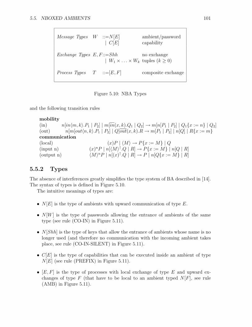
5.5. NBOXED AMBIENTS 101
Message Types W ::=N [E] ambient/password| C[E] capability
Exchange Types E,F ::=Shh no exchange| W1 × . . . × Wk tuples (k ≥ 0)
Process Types T ::=[E,F ] composite exchange
Figure 5.10: NBA Types
and the following transition rules
mobility
(in) n[in〈m, k〉.P1 | P2] | m[in(x, k).Q1 | Q2] → m[n[P1 | P2] | Q1{x := n} | Q2](out) n[m[out〈n, k〉.P1 | P2] | Q]out(x, k).R → m[P1 | P2] | n[Q] | R{x := m}communication
(local) (x)P | 〈M〉 → P{x := M} | Q(input n) (x)nP | n[〈M〉↑.Q | R] → P{x := M} | n[Q | R](output n) 〈M〉nP | n[(x)↑.Q | R] → P | n[Q{x := M} | R]
5.5.2 Types
The absence of interferences greatly simplifies the type system of BA described in [14].The syntax of types is defined in Figure 5.10.
The intuitive meanings of types are:
• N [E] is the type of ambients with upward communication of type E.
• N [W ] is the type of passwords allowing the entrance of ambients of the sametype (see rule (CO-IN) in Figure 5.11).
• N [Shh] is the type of keys that allow the entrance of ambients whose name is nolonger used (and therefore no communication with the incoming ambient takesplace, see rule (CO-IN-SILENT) in Figure 5.11).
• C[E] is the type of capabilities that can be executed inside an ambient of typeN [E] (see rule (PREFIX) in Figure 5.11).
• [E,F ] is the type of processes with local exchange of type E and upward ex-changes of type F (that have to be local to an ambient typed N [F ], see rule(AMB) in Figure 5.11).

102 CHAPTER 5. EXTENSIONS OF THE AMBIENT CALCULUS
(AMB) (PREFIX)
Γ ` M : N [E] Γ ` P : [F,E]
Γ ` M [P ] : [G,H]
Γ ` M : C[F ] Γ ` P : [E,G] F ∈ {Shh,G}
Γ ` M.P : [E,G]
(CO-IN) (CO-IN-SILENT)
Γ ` M : N [W ] Γ, x : N [W ] ` P : [E,F ]
Γ ` in(x,M).P : [E,F ]
Γ ` M : N [Shh] Γ ` P : [E,F ] (x 6∈ fv(P ))
Γ ` in(x,M).P : [E,F ]
(INPUT) (INPUT ↑)
Γ, x : W ` P : [W,E]
Γ ` (x : W ).P : [W,E]
Γ, x : W ` P : [E,W ]
Γ ` (x : W )↑.P : [E,W ](INPUT M)
Γ ` M : N [W ] Γ, x : W ` P : [G,H]
Γ ` (x : W )M .P : [G,H]
Figure 5.11: NBA Typing Rules

5.6. SEALED BOXED AMBIENTS 103
Rules for communication are similar to the ones in the previous section, withoutconsidering the security policy.
Unfortunately, all these intuitive meanings are not formalized.
5.6 Sealed Boxed Ambients
In [17] a first attempt to introduce cryptographic primitives within the Ambient Cal-culus framework can be found. The calculus of Sealed Boxed Ambients tries to reducethe degree of abstraction of the security model of AC, in the same way that the spi-calculus provides a lower level mechanism for the establishment of secure channels thanthe π-calculus. For instance, in the process
(νn)(a[n[out a.in b.〈m〉]] | b[open n.(x).P ])
no adversary can discover m, as it is encapsulated into the secret ambient n, but theambient enveloping mechanism is quite abstract. In a realistic scenario, name n willhave to be disclosed and, therefore, this message exchange protocol will no longer besafe. In [17] a key-based mechanism is proposed to formalize these ideas.
A specific primitive to let an ambient “seal” itself is introduced. By exercising thecapability seal k in one of its internal threads, an ambient n blocks all its interactionswith the outside and encrypts all its messages:
n[seal k.P | Q] → n�P | Q�k (5.5)
After the sealing of n, nor P nor Q can perform any communication action. How-ever, a sealed ambient may still move over the network until it reaches an ambientwhich knows the sealing key k. By means of coactions a la NBA the sealed ambient isgranted permission for migration and it becomes registered and unsealed:
n�in m.P | Q�k | m[in{x}k.R | S] → m[n[P | Q] | R{x := n} | S] (5.6)
5.6.1 Syntax and Semantics
The syntax of the SBA calculus is an extension of the NBA calculus in the previoussection. Its main novelties can be found in Figure 5.12.
The operational semantics of SBA is defined considering that ambients can be intwo states, either sealed or unsealed. We will write M{P} for M [P ] or M
�P �N , when
the distinction may be safely disregarded. The two states for reductions are formalizedby defining the reduction relation in terms of two inter-dependent relations (see Figure5.13).
The silent reduction relation 99K gives the semantics of mobility and sealing. Rules(in) and (out) allow any ambient to enter or exit any other ambient, while in rules (K-in) and (K-out) the incoming ambient is authenticated by a test on the sealing key andregistered by binding the variable. Silent reductions may occur within any context,

104 CHAPTER 5. EXTENSIONS OF THE AMBIENT CALCULUS
Expressions M,N ::=. . . | in | outPrefixes π ::=M | (x)η | 〈M〉η | in{x}M | out{x}M | seal MProcesses P ::=. . . | π.P | M [P ] | M
�P �N
Figure 5.12: SBA Syntax
except under prefixes. On the other hand, the reductions involving communicationmay only occur within unsealed ambients, as formalized by →. Note that its contextrule do not regard sealed ambients as a context. Rules (silent) and (ambient) guaranteethat the two reduction relations are linked properly.
5.6.2 Types
The type system developed for the SBA Calculus in [17] intends to protect the migrationof trusted code through untrusted sites. It will separate trusted and untrusted dataand code while allowing safe interactions with untrusted sites. The syntax of types isdefined in Figure 5.14.
The meaning of types is similar to the ones in the SBA Calculus in the previoussection. Amb[E] is the type of trusted ambients with upward communication of type E.Key[E] is the type of sealing keys that may be used to seal ambients of type Amb[E]:
Γ ` N : Key[E] Γ ` M : Amb[E] Γ ` P : [F,E]
Γ ` M�P �N : T
Γ ` M : Amb[E] Γ ` P : [F,E]
Γ ` M [P ] : T
Γ ` M : Key[E] Γ ` P : [F,E]
Γ ` seal M.P : [F,E]
Public data, of type Public, will be that coming from untrusted processes and hasto be carefully handled. For example, incoming data from a public ambient will beconsidered to be public:
Γ ` M : Public Γ, x : Public ` P : T
Γ ` (x)M .P : T
and viceversa, only public data can be sent to public ambients. However, both trustedand untrusted ambients can traverse any site, what is granted by the following rules:
Γ ` M : Public Γ ` P : TΓ ` M.P : T
M ∈ {in, out}
Γ ` M : Public

5.6. SEALED BOXED AMBIENTS 105
Silent reductionSilent reduction context S ::= − | (νs)S | P |S | n[S] | n�S�kMOBILITY (I)(in) n{in m.P | Q} | m{in.R | S}99Km{n{P | Q} | R | S}(out) m{n{out m.P | Q} | R} | out.S99Kn{P | Q} | m{R} | S
MOBILITY (II)
(K-in) n�in m.P | Q�k | m{in{x}k.R | S}99Km{n[P | Q] | R{x := n} | S}(K-out) m{P | n�out m.Q | R�k} | out{x}k.S99Km{P} | n[Q | R] | S{x := n}(seal) n[seal k.P | Q]99Kn�P | Q�kSTRUCTURAL RULES
(struct) P ≡ Q, Q 99K R, R ≡ S ⇒ P 99K S
(context) P 99K Q ⇒ S{P} 99K S{Q}
ReductionReduction context E ::= − | (νs)E | P |E | n[E]
COMMUNICATION
(local) (x)P | 〈M〉Q → P{x := M} | Q
(input n) (x)nP | n[〈M〉↑Q | R] → P{x := M} | n[Q | R](output n) 〈M〉nP | n[(x)↑Q | R] → P | n[Q{x := M} | R]
STRUCTURAL RULES
(silent) P 99K Q ⇒ P → Q
(ambient) P → Q ⇒ n[P ] 99K n[Q](struct) P ≡ Q, Q → R, R ≡ S ⇒ P → S
(context) P → Q ⇒ E{P} → E{Q}
Figure 5.13: Reduction and Silent Reduction for SBA
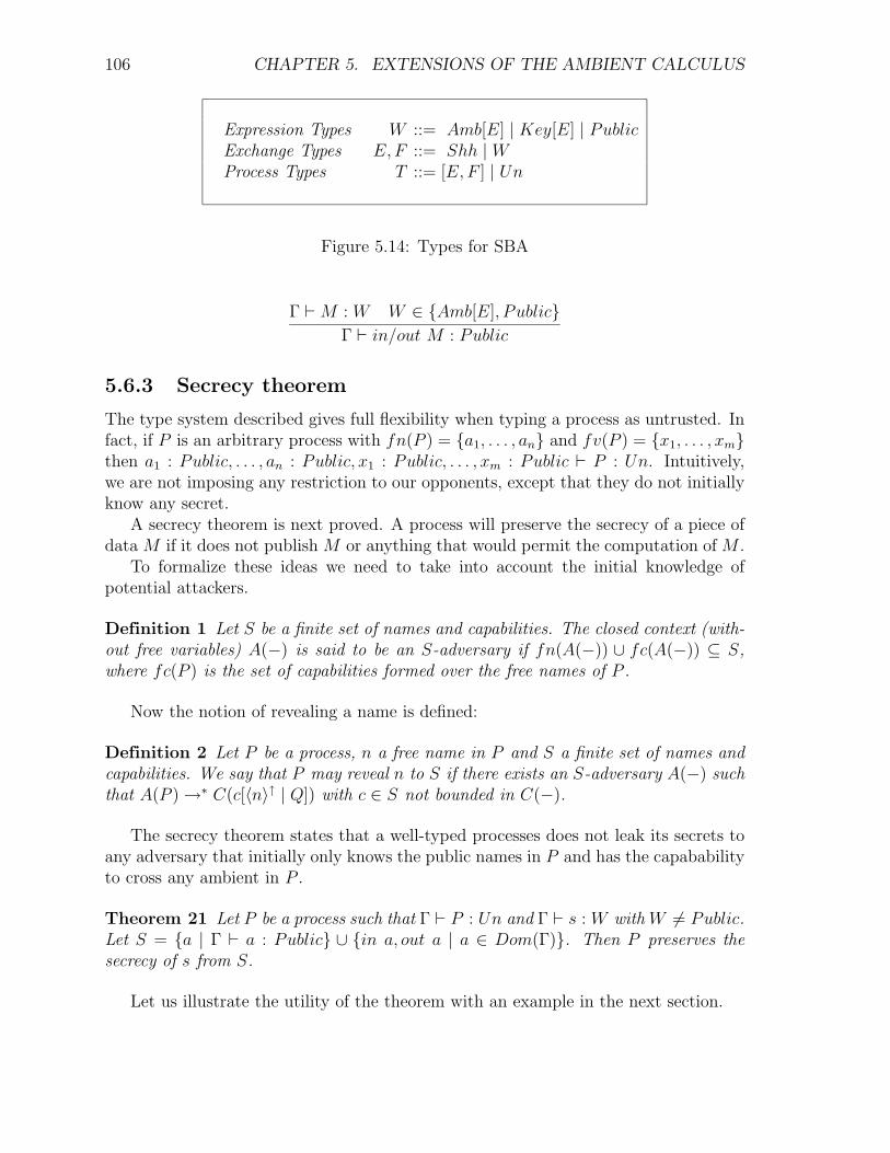
106 CHAPTER 5. EXTENSIONS OF THE AMBIENT CALCULUS
Expression Types W ::= Amb[E] | Key[E] | PublicExchange Types E,F ::= Shh | WProcess Types T ::= [E,F ] | Un
Figure 5.14: Types for SBA
Γ ` M : W W ∈ {Amb[E], Public}
Γ ` in/out M : Public
5.6.3 Secrecy theorem
The type system described gives full flexibility when typing a process as untrusted. Infact, if P is an arbitrary process with fn(P ) = {a1, . . . , an} and fv(P ) = {x1, . . . , xm}then a1 : Public, . . . , an : Public, x1 : Public, . . . , xm : Public ` P : Un. Intuitively,we are not imposing any restriction to our opponents, except that they do not initiallyknow any secret.
A secrecy theorem is next proved. A process will preserve the secrecy of a piece ofdata M if it does not publish M or anything that would permit the computation of M .
To formalize these ideas we need to take into account the initial knowledge ofpotential attackers.
Definition 1 Let S be a finite set of names and capabilities. The closed context (with-out free variables) A(−) is said to be an S-adversary if fn(A(−)) ∪ fc(A(−)) ⊆ S,where fc(P ) is the set of capabilities formed over the free names of P .
Now the notion of revealing a name is defined:
Definition 2 Let P be a process, n a free name in P and S a finite set of names andcapabilities. We say that P may reveal n to S if there exists an S-adversary A(−) suchthat A(P ) →∗ C(c[〈n〉↑ | Q]) with c ∈ S not bounded in C(−).
The secrecy theorem states that a well-typed processes does not leak its secrets toany adversary that initially only knows the public names in P and has the capababilityto cross any ambient in P .
Theorem 21 Let P be a process such that Γ ` P : Un and Γ ` s : W with W 6= Public.Let S = {a | Γ ` a : Public} ∪ {in a, out a | a ∈ Dom(Γ)}. Then P preserves thesecrecy of s from S.
Let us illustrate the utility of the theorem with an example in the next section.
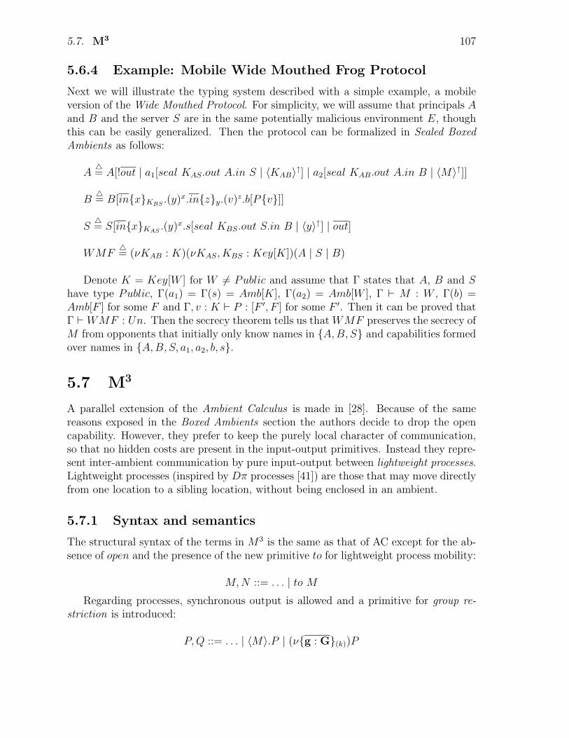
5.7. M3 107
5.6.4 Example: Mobile Wide Mouthed Frog Protocol
Next we will illustrate the typing system described with a simple example, a mobileversion of the Wide Mouthed Protocol. For simplicity, we will assume that principals Aand B and the server S are in the same potentially malicious environment E, thoughthis can be easily generalized. Then the protocol can be formalized in Sealed BoxedAmbients as follows:
A4= A[!out | a1[seal KAS.out A.in S | 〈KAB〉
↑] | a2[seal KAB.out A.in B | 〈M〉↑]]
B4= B[in{x}KBS
.(y)x.in{z}y.(v)z.b[P{v}]]
S4= S[in{x}KAS
.(y)x.s[seal KBS.out S.in B | 〈y〉↑] | out]
WMF4= (νKAB : K)(νKAS, KBS : Key[K])(A | S | B)
Denote K = Key[W ] for W 6= Public and assume that Γ states that A, B and Shave type Public, Γ(a1) = Γ(s) = Amb[K], Γ(a2) = Amb[W ], Γ ` M : W , Γ(b) =Amb[F ] for some F and Γ, v : K ` P : [F ′, F ] for some F ′. Then it can be proved thatΓ ` WMF : Un. Then the secrecy theorem tells us that WMF preserves the secrecy ofM from opponents that initially only know names in {A,B, S} and capabilities formedover names in {A,B, S, a1, a2, b, s}.
5.7 M3
A parallel extension of the Ambient Calculus is made in [28]. Because of the samereasons exposed in the Boxed Ambients section the authors decide to drop the opencapability. However, they prefer to keep the purely local character of communication,so that no hidden costs are present in the input-output primitives. Instead they repre-sent inter-ambient communication by pure input-output between lightweight processes.Lightweight processes (inspired by Dπ processes [41]) are those that may move directlyfrom one location to a sibling location, without being enclosed in an ambient.
5.7.1 Syntax and semantics
The structural syntax of the terms in M3 is the same as that of AC except for the ab-sence of open and the presence of the new primitive to for lightweight process mobility:
M,N ::= . . . | to M
Regarding processes, synchronous output is allowed and a primitive for group re-striction is introduced:
P,Q ::= . . . | 〈M〉.P | (ν{g : G}(k))P

108 CHAPTER 5. EXTENSIONS OF THE AMBIENT CALCULUS
g, h, . . . groupsS,C,E, . . . sets of groups, G is the universal set of groups
Amb::=amb(g) ambient type: ambients of group gPro ::=proc(g) process type: processes that can stay in ambients of group gCap ::=Pro1 → Pro2 capability type: capabilities that, prefixed to a process
of type Pro1, turn it into a process of type Pro2
W ::= message typeAmb ambient typeCap capability type
T ::= communication typeShh no communicationW communication of messages of type W
G ::=gr(S,C,E, T ) group type
Figure 5.15: M3 Types
where ν{g : G}(k) is a concise notation for ν{g1 : G1, . . . , gk : Gk}, the simultaneouscreation of groups. The syntax for types and group types will be defined in the nextsection.
Concerning the operational semantics it is only worth noting the rule for the newmobility primitive to:
n[to m.P | Q] | m[R] → n[Q] | m[P | Q] (R − to)
A lightweight process executing a to m action moves between sibling ambients:more precisely, it goes from an ambient n, where it is initially located, to a (different)ambient of name m that is a sibling of n, thus crossing two boundaries in one step(however, altogether, it does not change its nesting level) [28].
5.7.2 Types
The syntax of types is defined in Figure 5.15. The type system defined in this sec-tion will control communication and mobility, both ambient and process mobility.In order to do this but without using dependent types (with judgments of the formn : canEnter({m1, . . . ,mk})) a similar approach to that in [21] (already described inChapter 4) is taken, with the presence of groups. However, the approach is slightlydifferent. In [21] ambient types are essentially of the form amb(g,G)5, where G isthe expression of some properties concerning mobility and communication. Here, thecorresponding judgement would be less flexible: Γ ` m : amb(g) and Γ ` g : G, not
5In fact, following the same notation as in Chapter 4 the ambient type would be g[G]

5.7. M3 109
allowing different types for names in the same group. Therefore, all ambients belongingto group g will share the properties specified by G.
The intuitive meanings of types are the following:
• amb(g) is the type of ambients that belong to group g.
• proc(g) is the type of processes of type g, that is, processes that can safely runwithin ambients of type amb(g).
• proc(g1) → proc(g2) is the type of capabilities that, prefixed to a process oftype proc(g1), transform it into a process of type proc(g2) or, viewed at runtime,capabilities that, when exercised by a process of type proc(g2) (located in anambient of type amb(g2)), leave a continuation of type proc(g1) (located in anambient of type amb(g1)). Of course, it will be the case that g1 6= g2 only in thecase of the capability to.
• gr(S,C,E, T ), where S,C and E are sets of group names and T is a communicationtype; if g is a group of this type then the components have the following meaning:
– S is the set of ambient groups where the ambients of group g can stay;
– C is the set of ambient groups that ambients of group g can cross (it mustbe the case that C ⊆ S);
– E is the set of ambients that lightweight processes of type g can enter;
– T is the communication type within ambients of type g.
Now let us comment on some of the rules of the type system. If G = gr(S,C,E, T )is a group type we will write S(G), C(G), E(G) and T (G) respectively to denote thecomponents S, C, E and T of G. Moreover, whenever it is clear from the context wewill simply write g for amb(g) or proc(g) and g1 → g2 for proc(g1) → proc(g2). Rule(AMB)
Γ ` P : g Γ ` M : g Γ ` g : G g′ ∈ S(G)
Γ ` M [P ] : g′
states that the content process of an ambient must be of the same type as the ambientitself and that it can stay in ambients of any group g′ in S (which is exactly the set ofgroup names where ambients of type g can stay).
The most interesting rule for capabilities is the one for the primitive to:
Γ ` g2 : G2 Γ ` M : g1 g1 ∈ E(G2)
Γ ` to M : g1 → g2
It states that the action to m, performed by a process of group g2 leaves as contin-uation a process of group g1, if g1 is the group of m and one of the groups to which
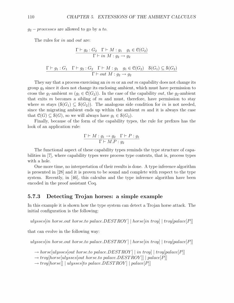
110 CHAPTER 5. EXTENSIONS OF THE AMBIENT CALCULUS
g2 − processes are allowed to go by a to.
The rules for in and out are:
Γ ` g2 : G2 Γ ` M : g1 g1 ∈ C(G2)
Γ ` in M : g2 → g2
Γ ` g1 : G1 Γ ` g2 : G2 Γ ` M : g1 g1 ∈ C(G2) S(G1) ⊆ S(G2)
Γ ` out M : g2 → g2
They say that a process exercising an in m or an out m capability does not change itsgroup g2 since it does not change its enclosing ambient, which must have permission tocross the g1-ambient m (g1 ∈ C(G2)). In the case of the capability out, the g2-ambientthat exits m becomes a sibling of m and must, therefore, have permission to staywhere m stays (S(G1) ⊆ S(G2)). The analogous side condition for in is not needed,since the migrating ambient ends up within the ambient m and it is always the casethat C(G) ⊆ S(G), so we will always have g1 ∈ S(G2).
Finally, because of the form of the capability types, the rule for prefixes has thelook of an application rule:
Γ ` M : g1 → g2 Γ ` P : g1
Γ ` M.P : g2
The functional aspect of these capability types reminds the type structure of capa-bilities in [7], where capability types were process type contexts, that is, process typeswith a hole.
One more time, no interpretation of their results is done. A type inference algorithmis presented in [28] and it is proven to be sound and complete with respect to the typesystem. Recently, in [46], this calculus and the type inference algorithm have beenencoded in the proof assistant Coq.
5.7.3 Detecting Trojan horses: a simple example
In this example it is shown how the type system can detect a Trojan horse attack. Theinitial configuration is the following:
ulysses[in horse.out horse.to palace.DESTROY ] | horse[in troy] | troy[palace[P ]]
that can evolve in the following way:
ulysses[in horse.out horse.to palace.DESTROY ] | horse[in troy] | troy[palace[P ]]
→ horse[ulysses[out horse.to palace.DESTROY ] | in troy] | troy[palace[P ]]→ troy[horse[ulysses[out horse.to palace.DESTROY ]] | palace[P ]]→ troy[horse[] | ulysses[to palace.DESTROY ] | palace[P ]]

5.7. M3 111
→ troy[horse[] | ulysses[] | palace[P | DESTROY ]]
Let us suppose that ambients ulysses, horse, . . . belong to groups gu, gh, . . . respec-tively and gm is the top-level ambient. Then, the initial process can be typed if theenvironment is such that Γ ` P : proc(gp), Γ ` DESTROY : proc(gp) and containsthe following assumptions:
gu : Gu = gr({gm, gt, gh}, {gh}, {gp}, Shh)gh : Gh = gr({gm, gt}, {gt}, φ, Shh)gt : Gt = gr({gm}, φ, φ, Shh)gp : Gp = gr({gt}, φ, φ, Shh)
Firstly,
Γ ` P : gt Γ ` palace : gp Γ ` gp : Gp gt ∈ S(Gp)
Γ ` palace[P ] : gt Γ ` troy : gt Γ ` gt : Gt gm ∈ S(Gt)
Γ ` troy[palace[P ]] : gm
Also,
Γ ` gh : Gh Γ ` troy : gt gt ∈ C(Gh)
Γ ` in troy : gh → gh Γ ` 0 : gh
Γ ` in troy.0 : gh Γ ` horse : gh Γ ` gh : Gh gm ∈ S(Gh)
Γ ` horse[in troy.0] : gm
We also have
Γ ` gu : Gu Γ ` horse : gh gh ∈ C(Gu)
Γ ` in horse : gu → gu
Γ ` gh : Gh Γ ` gu : Gu Γ ` horse : gh gh ∈ C(Gu) S(Gh) ⊆ S(Gu)
out horse : gu → gu
Γ ` gu : Gu Γ ` palace : gp gp ∈ E(Gu)
Γ ` to palace : gp → gu
and Γ ` DESTROY : gp. Then, applying several times the rule for prefixes we obtain
Γ ` in horse.out horse.to palace.DESTROY : gu
Finally, as gm ∈ S(Gu), we have
Γ ` ulysses[in horse.out horse.to palace.DESTROY ] : gm
and the whole process is typed.
112 CHAPTER 5. EXTENSIONS OF THE AMBIENT CALCULUS
Note that in order to type this process the following facts have played a crucial role:
· gt ∈ S(Gu), in order to fulfill the side condition S(Gh) ⊆ S(Gu) for the typing ofout horse, that is, Ulysses is allowed to stay in Troy.
· gp ∈ C(Gu), in order to type to palace, that is, Ulysses is allowed to cross thewalls of the palace.
Without these two assumptions (hardly assumable by Trojans) the process couldhave not been successfully typed.

Chapter 6
Operational Interpretation of
Results
In this chapter we will propose a general method for the treatment of history-dependantruntime errors. When one has to control this kind of errors, a tagged version of thelanguage is usually defined, in which tags capture only the needed information of thehistory of processes. We will characterize such languages as being quotients of thereachability tree defined by the transition graph. This fact tells us that the propertycharacterized by the tagged language is indeed a property of the original one, thusmaintaining an homogeneous framework instead of defining an ad-hoc semantics foreach property. In particular, we could still use the analysis machinery existing in thecalculus in order to prove that or other related properties.
6.1 Tagged Transitions Systems
In this section we will formally define what a tagged language will be for us. We startby defining the tagged syntax generated by a given many-sorted signature [32, 39] (aset of formal functional symbols with an associated arity), with respect to a symbol ofthe signature and the considered set of labels:
Definition 3 Given a many-sorted signature (S, Σ), let E be the S-sorted term algebraof Σ, f a symbol of Σ and L a set of labels (Γ, ∆, . . . ∈ L). We will call (f,L)-taggedsyntax of E, and we will denote it by EL
f (or sometimes just by E), to the S-sorted
term algebra of ΣL
f = (Σ − {f}) ∪ {fΓ|Γ ∈ L}, where arity(fΓ) = arity(f) for everyΓ ∈ L.
In terms of abstract syntax trees, tagged terms are usual terms where some nodes,that are leaves in case the distinguished symbol f is a constant operator, or internalnodes otherwise, are annotated with labels in L. A more general version of taggedsyntax, EL1,L2,...
f1,f2,... , would consider a collection of symbols f1, f2, . . . in Σ, and a (possibly)different set of labels for each one of them.
113

114 CHAPTER 6. OPERATIONAL INTERPRETATION OF RESULTS
+
Succ
Zero
×
Zero Succ
Zero
+
Succ
Zero
×
Zero Succ
Zero
Figure 6.1: Abstract syntax trees for 1 + (0 × 1) and 1 ⊕ (0� 1)
Example 1 Let us consider (S, Σ), where Σ = {Zero, Succ, +,×} and S = {Nat}with arity(Zero) = Nat, arity(Succ) = Nat → Nat and arity(+) = arity(×) =Nat → Nat → Nat; and the set of labels L = {�,◦}. The S-sorted term algebraof Σ defines a set of arithmetic expressions. One tagged syntax is that generated byΣL,L
+,× = {Zero, Succ,⊕,⊗,�,�}, which defines ordinary expressions in which the op-eration symbols are substituted by “encircled” or “framed” symbols. Figure 6.1 showsthe abstract syntax trees of expressions 1 + (0 × 1) and 1 ⊕ (0� 1).
We will use the usual definition of labelled transition system:
Definition 4 A labelled transition system S is a tuple S = (E, V,→, e0), where Eis the set of states, V is the set of transition labels, e0 ∈ E is the initial state and→⊂ E × V × E is the transition relation. If (e1, a, e2) ∈→ we will write e1
a→ e2.
We will write e →∗ e′ if there exists s = a1 ·. . .·an such that ea1→ e1
a2→ . . .an→ en = e′
and we will take Reach(S) = {e ∈ E | e0 →∗ e}, the set of reachable terms. For ourpurposes, we will say that two transition systems are isomorphic if they are equal upto renaming of states, disregarding non reachable terms:
Definition 5 Let S = (E, V,→, e0) and T = (F, V, 7→, f0) be two labelled transi-tion systems. We will say that S and T are isomorphic if there exists a mappingh : Reach(S) → Reach(T ) such that:
1. h is a bijection
2. h(e0) = f0
3. ea→ e′ ⇔ h(e)
a7→ h(e′) for all e ∈ Reach(S)

6.1. TAGGED TRANSITIONS SYSTEMS 115
Now we will define when a transition system over the tagged syntax is a tagging ofthe original transition system. In this definition we will use the notation O(e) for theterm obtained from a tagged term e once we have removed all the tags in it.
Definition 6 Let E be the S-sorted term algebra of Σ and E a (f,L)-tagged syntaxof E. Also let S = (E, V,→, e0) and T = (E, V, 7→, e0) be two transition systems withO(e0) = e0. We will say that T is a tagging of S if the following conditions hold:
1. If ea7→ e′ then O(e)
a→ O(e′).
2. If ea→ e′ then for all e reachable from e0 such that O(e) = e there exists a unique
e′ with O(e′) = e′ such that ea7→ e′.
The first condition is a correctness property on tagged systems: they do not intro-duce new transitions, that is, all their transitions come from an untagged one. Thesecond is a completeness condition: we have a unique tagged version for each origi-nal transition. The uniqueness intuitively states that we cannot separately rememberdifferent things about the same past.
Example 2 Let us consider S = {Nat}, Σ = {1, 2, 3, 4, 5} with arity(i) = Nat andthe set of tags L = {◦,2}. The terms obtained when we tag every terminal symbolwith L, are just the elements in {1, . . . , 5} encircled by ◦ or 2. Now let us considerthe transition system defined by the following graph:
1
2
3 4
5
In this simple example, in which the graph defining the transition system is in facta tree, a tagged system will consist on several copies of the original system, at mostone for each way of annotating the initial symbol, like in the following examples:
1
2
3 4
5
1
2
3 4
5
1
2
3 4
5

116 CHAPTER 6. OPERATIONAL INTERPRETATION OF RESULTS
However, these copies could partially overlap for non-reachable terms, getting forinstance:
1
2
3 4
5
1
2
3
1
2
3 4
5
1
2
Notice that we allow in the definition of tagged systems the existence of somegarbage nodes (under certain conditions), that will not be reachable from the initialstate. We do this to get a more flexible definition of tagged systems, so that we donot need an exact knowledge of the set of reachable terms to define a tagged system.Of course, in practice, we will try to define them with the least possible amount ofgarbage, in order to simplify them as much as possible.1
Note that all these tagged systems are indeed isomorphic: if we remove everynon reachable term they become equal, except for the name of states. This mustbe the case in this example because the transition graph is a tree and, therefore, eachnode determines a unique path from the initial node (the transition graph and thereachability tree are isomorphic). As a different example, let us consider the transitionsystem defined by the graph on the left of the following figure, that is not a tree. Thecorresponding tagged systems on the right can now discriminate between different waysof reaching state 3, although the one in the middle forgets this difference once we moveinto state 2.
1
2 3
1
2 3
3
1
2 3
3 2
It is the existence of several reachable nodes with different labels what makes labelsvaluable: just by checking the label in the reached state we have a (partial) knowledgeof the way we reached that node.
1Garbage nodes are useless, but at the same time they are absolutely innocuous, out of the in-creasing of the size of the system.
6.2. ALTERNATIVE CHARACTERIZATION OF TAGGED SYSTEMS 117
6.2 Alternative characterization of tagged systems
In this section we will characterize the tagged systems defined in the previous sectionas quotients of its reachability tree. To be more precise, tagged systems are isomorphic(in the sense we have defined) to the computation tree, once we have identified someof its nodes. We start by defining the computation tree:
Definition 7 Given S = (E, V,→, e0) a labelled transition system and C the set ofcomputation sequences of S we define the corresponding computation tree St = (C, V, 7→, e0),as the transition system obtained taking 7→⊂ C × V × C defined by the rule:
ea→ e′ last(L) = e
La7→ (L
a→ e′)
where “last” is the function that gives us the last state of each computation sequence.
The computation tree is simply the transition system defined by the reachabilitytree of the original system. It merely accumulates in its states the sequence of statesthat have been visited along the computation and the transitions between them. Thus,it contains all the information about the history of the process. We will sometimes callit the totally tagged system.
However, in general we will only be interested in a particular aspect of this in-formation. We will use equivalence relations among computations to identify thatinformation.
Definition 8 We will say an equivalence relation ∼⊂ C × C is suitable if it satisfiesthe following conditions:
1. L1, L2 ∈ C and L1 ∼ L2 ⇒ (L1a→ e) ∼ (L2
a→ e)
2. L1 ∼ L2 ⇒ last(L1) = last(L2)
For example the relations ∼⊥ such that L1 ∼⊥ L2 ⇔ last(L1) = last(L2) and ∼>
such that L1 ∼> L2 ⇔ L1 = L2 are trivial examples of suitable equivalences.By means of the suitable equivalences we will characterize the information about
the past we are interested in. For instance, ∼⊥ is the relation that forgets everythingabout the past, while ∼> is the one remembering absolutely everything. Now we definethe quotient transition system generated by such an equivalence relation:
Definition 9 Let S = (E, V,→, e0) be a labelled transition system and ∼⊂ C × C asuitable equivalence relation. We define S∼ = (C/∼, V, 7→∼, [e0]), and call it a quotienttransition system of S with respect to ∼, as the transition system defined by the rule
La7→ L′
[L]a7→∼ [L′]

118 CHAPTER 6. OPERATIONAL INTERPRETATION OF RESULTS
e1 e2 e3
e1 e2 e3
a b
a b
π π π
Figure 6.2: Commutative diagram induced by a quotient transition system
The first condition over ∼ indicates us that the quotient transition system is uni-formly defined, in the sense that its transitions do not depend on the election of therepresentatives of the equivalence classes. The second states that the relation remindsat least the final state reached by the computation. These conditions induce a com-mutative diagram for every computation sequence, as illustrated in Figure 6.2. In thisdiagram, function π is the quotient map, which is defined over the computation se-quence reaching each ei.
Quotient transition systems are a conservative extension of ordinary transition sys-tems in the following sense:
Proposition 22 If [L1], [L2] ∈ C/∼ and [L1]a7→∼ [L2] then last(L1)
a→ last(L2)
Proof. Let us suppose that [L1]a7→∼ [L2]. By definition of 7→∼ there exist L′
1
and L′2 such that L1 ∼ L′
1, L2 ∼ L′2 and L′
1a7→ L′
2. As well, by definition of 7→, itholds that last(L′
1)a7→ last(L′
2) and, since ∼ was suitable and Li ∼ L′i, it follows that
last(Li) = last(L′i) and, therefore, we are done.
2
Now let us take a closer view at the structure of the set of quotient transitionsystems.
Definition 10 We denote by S the set of quotient transition systems, S = {S∼ |∼ suitable},
and define the operators S∼1 tS∼24= S∼1∩∼2 and S∼1 uS∼2
4= S∼1∪∗∼2, where R1∪
∗ R2
denotes the transitive closure of R1 ∪ R2.
Then we have the following proposition:
Proposition 23 (S,u,t) is a complete lattice that has S and St as bottom and topelements, respectively.
Proof. First, (S,u,t) is a lattice, since both u and t are idempotent, commutative,associative and satisfy the absorption law. To prove that it is complete we have to

6.2. ALTERNATIVE CHARACTERIZATION OF TAGGED SYSTEMS 119
see that every subset of S has a supremum and an infimum. Let {S∼i | i ∈ I} bea subset of S and take ∼inf=
⋃∗i∈I ∼i and ∼sup=
⋂
i∈I ∼i. Both ∼inf and ∼sup aresuitable equivalence relations and S∼inf and S∼sup are the infimum and the supremum of{S∼i | i ∈ I}, respectively. Also, if ∼ is a suitable equivalence relation then ∼>⊆∼⊆∼⊥
and, therefore S∼⊥ � S∼ � S∼> . To conclude, it remains to see that S and St
are isomorphic to S∼⊥ and S∼> respectively. The latter is trivial. Let us see theformer. We take h(e) = [e]∼⊥
for e ∈ E, that is, the quotient mapping restricted toempty computations sequences. Let us see that h is a bijection satisfying the requiredcondition. h is bijective since it is the inverse of last([L]∼⊥
) = last(L), that does notdepend on the chosen representative of [L], since ∼⊥ is suitable. Indeed, it holds thatlast ◦ h = IdE and h ◦ last = IdC/∼
⊥
and since [ea→ e′]∼⊥
= [e′]∼⊥, it follows that
ea→ e′ ⇔ h(e)
a7→ h(e′), for all e ∈ Reach(S).
2
Now let us state the main theorem of this section:
Proposition 24 Let S = (E, V,→, e0) be a labelled transition system and let us con-sider T = (E, V, 7→, e0) a tagging of S. Then T is isomorphic to a quotient transitionsystem of S.
Proof. Let us suppose that T is a tagging of S. We must find a suitable relation∼, such that T will be isomorphic to S∼. We will get it by defining a function π over
the computation sequences of S, and taking ∼ as the kernel of π (that is, L1 ∼ L24⇔
π(L1) = π(L2)). For each computation L, we define π(L) by induction on its length.The base case is straightforward, π(e0) = e0. Let us suppose that we have just definedπ(L) = e and we want to define π(L
a→ e′). Since e
a→ e′ and O(e) = e, there exists
a single e′ satisfying condition 2 of the definition of tagged systems. Then we takeπ(L
a→ e′) = e′.
It is easy to see that the so defined relation is suitable and that T is isomorphicto S∼. It suffices to take h([L]) = π(L), that is well defined by definition of ∼, is abijection between reachable terms and satisfies the conditions to be an isomorphismbetween transition systems.
2
The reciprocal is also true:
Proposition 25 Let S = (E, V,→, e0) be a labelled transition system and ∼ a suitableequivalence relation. Then S∼ is isomorphic to a tagging of S.
Proof. Let S = (E, V,→, e0) be a labelled transition system and ∼ a suitablerelation over its computation sequences. We must define a tagging of S, S, isomorphicto S∼. First, we will tag every term of the syntax, so that tagged terms can be seen

120 CHAPTER 6. OPERATIONAL INTERPRETATION OF RESULTS
as pairs (e, Γ) with e ∈ E. Now, we take as set of labels the set C/∼ of equivalenceclasses defined by the suitable relation ∼. Then we define 7→ by the rule
ea→ e′ last(L) = e
(e, [L])a7→ (e′, [L
a→ e′])
The transition relation 7→ is well defined since ∼ is suitable. In the way we have definedit, it holds that S = (E × C/∼, V, 7→, (e0, [e0])) is a tagging of S. To conclude the proof,we just have to check that the function h([L]) = (last(L), [L]) defines an isomorphismbetween S and S∼, what is immediate.
2
In our Example 2 the lattice generated by the transition system is degenerate, sincethe bottom and the top elements are isomorphic. Therefore, all the tagged systems arealso isomorphic. Let us study a more interesting example:
Example 3 Let us consider another toy example using the language Dπ. Let us takethe process `
�∗(go κ.go `)� which spawns agents that go to location κ and back to `,
where they die. We will take the set of labels L = {�,◦} to label the transition systemthat the term generates. For each natural number let n = κ
�go `� | n. . . | κ
�go `� |
`�∗(go κ.go `)�, be the term that represents the state in which exactly n agents are at
κ. Then we can present the transition graph and the corresponding reachability tree inthe following way:
0
1
2
3
...
Quotienttransition systems
0
01
010 012
0101 0121 0123
...
Now the following two transition graphs define a couple of quotient transition sys-tems. The one on the left determines the parity of the number of agents that have died.The one on the right only determines whether any agent has ever died. More precisely,in this case state n corresponds to computation 01 . . . n, while state n identifiesevery computation sequence ending in state n, but 01 . . . n. In terms of the used suit-able relation, ∼ identifies only with itself every computation of the form 01 . . . n (theright-branch of the reachability tree), while for the rest of the nodes, it relates everycomputation ending in the same state.

6.3. DERIVING TAGGED LANGUAGES 121
0
1
2
3
0
1
2
3
...
0
1
2
3
0
1
2
3
...
6.3 Deriving Tagged Languages
Now we address the problem of deciding whether an operational semantics, defined bya reduction relation over a tagged syntax is in fact a tagging (and therefore a quotient)of the original semantics.
Tagged semantics will be parameterized over the set of possible initial taggingfunctions tag : E → E, that will depend on the specific application we are interestedin. In particular, tagging functions will satisfy O ◦ tag = IdE, but not the other wayaround. Typically, this function will capture on tags the static information needed toformalize the property in which we are interested.
In general, a semantics over the tagged syntax is a tagging of another operationalsemantics with respect to an initial tagging function tag if for every P the transitionsystem that generates tag(P ) is a tagging of the transition system generated by P :
Definition 11 We will say that a reduction relation R = (E, V, 7→) is a tagging ofR = (E, V,→) with respect to the initial tagging function tag if for every e ∈ E thelabelled transition system (E, V, 7→, tag(e)) is a tagging of (E, V,→, e)
We will just consider a particular case, that will be enough for our current purposes,this in which the reduction relation is structurally defined. Let us suppose that → isdefined by means of a set of axioms Ai : Pi
ai→ Qi for i = 1, 2, . . . and a set of structuralrules Ri of the form
Pa→ Q
Ci(P )a→ Ci(Q)
with contexts Ci = f i(t1, ..,�, .., tni), i = 1, 2, . . ., where the f i’s used in the contexts
are not distinguished symbols. Then, these structural rules can be directly consideredas rules for the tagged syntax. In this setting, if we replace every axiom by the set ofcorresponding tagged versions for every way of tagging the Pi’s, we obtain a taggingof R:
122 CHAPTER 6. OPERATIONAL INTERPRETATION OF RESULTS
Proposition 26 Let us consider R as above and a set of axioms Ai : P iai7→ Qi, with
i = 1, 2, . . ., such that O(P i) = Pi and O(Qi) = Qi; assume that each Ai is definedfor every possible tagging of Pi
2. Let R be the reduction relation defined by the set ofaxioms A1, A2, . . . and the set of compositional rules R1, R2, . . . Then R is a tagging ofR.
Proof. Given P0, we prove condition 1 by rule induction on the definition of 7→ andcondition 2 by rule induction on the definition of →:
1. If Pa7→ P ′ then O(P )
a→ O(P ′)
(a) Ai : Piai7→ Qi. By hypothesis Ai : O(Pi)
ai7→ O(Qi).
(b) For the sake of readability, let us suppose that Ri : P = f i(Q)a7→ f i(Q′) =
P ′ with Qa7→ Q′. By induction hypothesis we have O(Q)
a→ O(Q′). Since
the symbol f i is not distinguished, O(P ) = O(f i(Q)) = f i(O(Q)), and wecan apply rule Ri to obtain O(P ) = f i(O(Q))
a→ f i(O(Q′)) = O(f i(Q′)) =
O(P ′).
2. If Pa→ P ′ and P ∈ Reach(tag(P0)) such that O(P ) = P then there exists a
unique P ′ with O(P ′) = P ′ and Pa7→ P ′:
(a) Ai : Piai→ Qi. By hypothesis, for every tagging Pi of Pi we have a unique
tagged version of the axiom, Ai.
(b) Again for the sake of readability, let us suppose that P = f i(Q)a→ P ′ =
f i(Q′) with Qa→ Q′. Given P as above, since f i is not distinguished, it
must be the case that P = f i(Q) with O(Q) = Q. Now we can apply theinduction hypothesis: there exists a unique Q′ such that O(Q′) = Q′ andQ
a7→ Q′. Now we can take P ′ = f i(Q′), that is the only term such that
O(P ′) = P ′ and Pa7→ P ′.
2
This is the simplest way of deriving a tagged semantics from a given semantics.The same can be done if it is also defined by means of a structural congruence if thedistinguished symbols do not appear either in its axioms or in the rules. In this casethese axioms and rules can be also applied to the tagged relation, thus defining astructural equivalence between tagged terms. Then, if we add to the set of previousreduction rules the corresponding structural rule we also obtain a tagging of the originalsemantics. This is exactly the case we will study in the following section.
2In a more formal way, we could have an axiom Ai,P i: P i
ai→ Qi for each P i such that O(P i) = Pi,but usually they will all have a homogenous structure.
6.4. TAGGED Dπ 123
6.4 Tagged Dπ
In this section we will see how the proposed methodology can be applied to the languageDπ presented in Chapter 23.
To see that the tagged language defined in [41] is a tagging of the original languageit suffices to see that it can be defined in the way described in the previous section.
The set L of tags will be the set of partial functions from locality identifiers to K,the set of open locality types, as seen in Chapter 2. The distinguished symbol is thatdefining agents,
� �. By mere inspection of the rules defining the tagged language itcan be seen that they conform to the conditions considered in the previous section.Indeed, we have a tagged version of each axiom, for every way of tagging the term onits left hand-side. The rest of the rules of the original language can also be consideredas rules of the tagged one, since the symbol
� � does not appear in their definition.Then we have the following
Theorem 27 The tagged Dπ is indeed a tagging of Dπ
According to this result and our characterization of tagged systems it follows thatthe transition system generated by each term of Tagged Dπ is isomorphic to a quotienttransition system. Therefore, every property defined over Tagged Dπ is also a propertyof Dπ. In particular, every subset of tagged terms (e.g., that of erroneous terms) definesa subset of computations (that of erroneous computations).
The result is true whatever the initial tagging function is. However, the electionis crucial to adequately formalize the runtime errors we have in mind: in this casethe resource access errors. In [41] the chosen function tag is only defined for typedprocesses of the original calculus, so that if M is not typeable then tag(M) = ∅.Another possibility is to tag every original process, simply by adding in the tags thecreated names, which are exactly those the agents have initially permission to use. Wewill do so with the help of the mappings tagΓ(M), where Γ is the initial knowledge of M .Let us consider the system (νa : A)(k
�b!〈a〉� | k
�b?(x : A).x!〈c〉�) Though the channel
a is created with the two agents under its scope, only the agent on the left knows of itsexistence. In fact, the scope of the names can always be extended via extrusion. Forinstance, that system and (νa : A)k
�b!〈a〉� | k
�b?(x : A).x!〈c〉� are equivalent. In order
to deal with this fact, we will restrict ambient domains in tagΓ(M) to the set of freenames in M , that is, we will have the invariant dom(Γ) = fn(M), and we will denoteby ΓM the restriction Γ |M . Now we can define the initial tagging function:
Definition 12 Let Φ be the empty (partial) function in L (that with empty domain).Then we define the function tag : M → M by:
• tag(M) = tagΦ(M) if M is closed
3In fact, we see it for the language in which all the rules presented of the structural congruence,but S-EXTR and S-GARB1, have been turned into reduction rules
124 CHAPTER 6. OPERATIONAL INTERPRETATION OF RESULTS
• tagΓ(0) = 0
• tagΓ(M | N) = tagΓM(M) | tagΓN
(N)
• tagΓ((ν`e : E)M) = (ν`e : E)tagΓ,{`e:E}(M) if e ∈ fn(M)
• tagΓ((ν`e : E)M) = (ν`e : E)tagΓ(M) if e 6∈ fn(M)
• tagΓ(`�P �) = `
�P �Γ
In [41] an error relation on the corresponding tagged systems M → err is defined,meaning that a process can violate its permissions. To remove these errors, a typesystem ` for the original language and another related one for the tagged systemswere defined. We need the following lemma:
Lemma 28 If Γ ` M then Γ tagΓ(M)
Proof. The proof is straightforward by induction on the rules used to derive Γ ` M :
1. Γ ` 0. Since tagΓ(0) = 0 and Γ 0 the thesis follows.
2. Γ ` k�P �. Then it is the case that Γ `k P . Since Γ <: Γ it follows that Γ k
�P �.
3. Γ ` M1 | M2 with Γ ` Mi. By strengthening it follows that ΓMi` Mi and
by induction hypothesis, ΓMi tagΓMi
(Mi) and, by weakening, Γ tagΓMi(Mi).
Since tagΓ(M1 | M2) = tagΓM1(M1) | tagΓM2
(M2) it follows that Γ tagΓ(M1 |M2).
4. Γ ` (νke : E)M with Γ, {ke : E} ` M . By induction hypothesis it follows thatΓ, {ke : E} tagΓ,{ke:E}(M)
(a) If e ∈ fn(M) then tag((νke : E)M) = (νke : E)tagΓ,{ke:E}(M) and we canconclude Γ tagΓ((νke : E)M)
(b) If e /∈ fn(M) then by strengthening it also holds that Γ tagΓ,{ke:E}(M)and since in that case tag((νke : E)M) = (νke : E)tagΓ,{ke:E}(M), the thesisfollows.
2
The result is also said to be true in [41] but since there no formal relation betweenboth languages was established, then the corresponding proof should rephrase for thisparticular case the relations that are guaranteed by our tagging framework.
A subject reduction theorem and a safety theorem for the tagged system wereproved in [41]. Then we have our safety theorem:
Theorem 29 If Γ ` M and tagΓ(M) 7→∗ M ′ then M ′ 6→ err

6.4. TAGGED Dπ 125
and the following
Corolary 30 If Φ ` M and tag(M) 7→∗ M ′ then M ′ 6→ err
This result also appears in [41], but no interpretation of it is given in terms of theoriginal semantics of the language. Instead we can now interpret the fact that M 6→ erras the impossibility to use a resource when we have not received the permission to doit along the current computation, since the tags exactly remind the set of accumulatedpermissions.
Example 4 As a very simple example, let us consider
M = (ν` : loc{a : res〈T 〉})(νkb : res〈T 〉)(ν`c : T )`�b!〈c〉�
We can tag M , getting
tag(M) = (ν` : loc{a : res〈T 〉})(νkb : res〈T 〉)(ν`c : T )`�b!〈c〉�Γ
withΓ = {` : loc{a : res〈T 〉, c : T}, k : loc{b : res〈T 〉}}
However, M is not typeable and, in fact, tag(M) → err, since it attempts to usechannel b at locality l, what is not allowed by Γ. Of course, since types cannot becomplete, it could be the case that M is not typeable but tag(M) will not produce anyerror.

126 CHAPTER 6. OPERATIONAL INTERPRETATION OF RESULTS
Chapter 7
Conclusions and future work
In the present work we have studied several type-based approaches to the analysis offormal models for mobile systems. We have described the state of the art at the currentstage, starting from the π-calculus and its derivates to focus then on the AmbientCalculus and some of its extensions with the aid of examples, some original and sometaken out from the papers.
Some other related works that we have also considered but we decided not to in-clude in this work in order to avoid it from growing more than desired, are the JoinCalculus [35], the Seal Calculus [69], KLAIM [30] or λπv [73].
We have found that in many cases just a type system was defined, without definingthe property of the semantics it was intended to capture. This happened, in particular,in the original papers for the Ambient Calculus, though in these cases the correspond-ing definition is simple, due to the simplicity of the considered properties. We have
formalized them through a set of unary relationsΓ→ erri, (i = 1, 2, 3, 4) on processes
that represent the occurrence of runtime errors. In this case, these exceptions could bestatically spotted when the error-prone state was reached. First a syntactic error err1
was defined, that was independent of the current security policy and then some others(that subsumed the first one) for communication, err2, mobility and opening control,err3, and mobility and opening control with groups, err4. We have also introduced atype system that can deal with more than one single blackboard, one for each arity,and a notion of associated error.
Regarding the types for the Ambient Calculus with groups, they can be consideredas objective types, since they specify the permissions ambients have with respect to thegroups. Maybe it would be interesting to develop a dual subjective vision of types, inwhich types specify the permissions ambients offer to groups. This type system shouldtake into account the possible dynamic ambient topology of processes or even rely onan analysis approximating such structure, as the ones developed in [47] or in [58].
Another contribution of our work has been a rather simple but conceptually impor-tant justification of the use of tagged languages for the analysis of our systems. The
127

128 CHAPTER 7. CONCLUSIONS AND FUTURE WORK
fact that these systems are quotients of the corresponding reachability tree tells us thatthe properties defined over them are, in fact, also properties of the original semantics,thus keeping us within the same original framework for every possible property of ourinterest. It may also be worthy a further study of the algebraic structure of the set oftagged languages and exploit it for the combination of properties. For example, if wehave a language tagged with L and an injective mapping L ↪→ L′ then we can considerthe language as being tagged with L′. Therefore, if we have tagged a language in twodifferent ways, say with L1 and L2 to treat two different properties we can considerL = L1 ×L2 and consider both tagged languages as two different taggings in the sametagged syntax. Then we can consider the language satisfying both properties simulta-neously. If ∼1 and ∼2 were the equivalence relations defining each property then thecorresponding tagged language would be S∼1 t S∼2 .
Let us remember the Example 3 in Chapter 6. If we want to consider the con-junction of both properties (whether any agent has died, in which case, whether ithas been in an even or an odd number) it suffices to consider L = {�,◦} × {�,◦}and the corresponding joint transition system. If we denote ◦ = (◦,◦), � = (�,�)and � = (◦,�) (we will not need tag (�,◦) since terms tagged with it will not bereachable) then we have:
0
1
2
3
0
1
2
3
...
0
1
2
3
0
1
2
3
...
t =
0
1
2
3
0
1
2
3
...
0
1
2
3
...
where terms tagged with ◦ identify computations in which no agent has died, � identi-fies computations in which an odd number of agents have died and � identifies compu-tations in which an even, but greater than zero, number of agents have died. However,when we consider the meet of both transition systems (the disjunction of properties)we go all the way down to the bottom of the lattice:
0
1
2
3
0
1
2
3
...
0
1
2
3
0
1
2
3
...
u =
0
1
2
3
...

129
S
St
S
⊥S
Figure 7.1: Extended quotient systems lattice
So far, we have considered equivalences reminding at least the reached state, thusgetting always some tagged systems. However, this constraint could be relaxed toobtain a superset of our class of quotient systems (see Figure 7). Then the bottomwould represent the tagged system forgetting absolutely everything, even the reachedstate. Additionally, we would have transition systems lying in the diamond of thebottom of Figure 8, remembering only certain properties about the reached state, andtransition systems combining both approaches, the ones in the diamonds at both sidesof the figure, that remember some things about the past of the process but still onlypart of the information about the reached state.
Other field which could be worth studying in more detail is that of mobile cryptogra-phy. Current models supporting cryptography in this setting assume that cyphertextsare frozen pieces of code, that are defrosted at decoding. However, some recent researchin this field is concentrating on the possibility of computing with encrypted code andencrypted data. Therefore, we need models for analyzing these systems. For it we pro-pose a new calculus, that we will call SAC (Security Ambient Calculus). It is based onthe original Ambient Calculus, although coactions could also be considered. However,messages can be encrypted using a public-key cryptosystem such as RSA. The modeluses a function ( ·−1) : K 7→ K−1, such that if K is a public key then K−1 is thecorresponding private key and viceversa. The special case when K−1 = K for everyK can be used to model a symmetric cryptosystem, such as DES. Then a primitivefor input and decoding is introduced. In order to make the language more interesting,additional functionality is added to messages. The resulting tentative syntax is thatpresented in Figure 7.2.
For the definition of the semantics a subset of value expressions and evaluationcontexts for expressions and processes are defined, as done in [7]. Note that evalua-tion contexts impose an order on the evaluation of expressions. For example, in anapplication the function must be evaluated in the first place and then the argument.Only then, when both the λ-abstraction and the argument have been evaluated, thereduction proceeds using β-reduction. The definition of the structural equivalence isstandard. The reduction relation is defined in Figure 7.3.

130 CHAPTER 7. CONCLUSIONS AND FUTURE WORK
Processes: Expressions:P ::= 0 process nil M ::= k | n keys - names
P1 | P2 parallel composition ε empty path(νn)P name restriction x variables!P replication in M enterM [P ] ambient out M exitM.P prefix open M opening〈M〉 output M1.M2 path(x).P input {M}K cyphertext(x)M .P input+decoding λx.M λ-abstraction
M1M2 application. . .
Figure 7.2: The SAC Calculus
Values
V ::=n | λx.M | ε | V1.V2 | in V | out V | open V
Evaluation Contexts
E ::=�e | EM | V E | E.M | V.E | {E}K | in E | out E | open E
Process Evaluation Contexts
P ::=�p | E.P | E[P ] | 〈E〉 | (νn)P | n[P] | P | P
Reduction Rules
(Beta) (λx.M)V → M{x := V }(E-Str) M1 → M2 ⇒ E(M1) → E(M2)
(Usual reductions for movement and local communication)
(Exp-Ctx) M1 → M2 ⇒ P(M1)e → P(M2)e
(Proc-Ctx) P → Q ⇒ P(P )p → P(Q)p
(Dec) 〈{M}K〉 | (x)K−1 .P → P{x := M}(Str) P ≡ P ′ → Q′ ≡ Q ⇒ P → Q
Figure 7.3: SAC Reduction Relation

131
Using this language we can write the following version of the WMF protocol:
A4= A[a1[out A.in S | 〈{KAB}KAS
〉] | a2[out A.in B | 〈{M}KAB〉]]
B4= B[open a2 | open s.(x)KBS
.(y)xP{y}]
S4= S[open a1.(x)KAS
.s[〈{x}〉KBS| out S.in B]]
WMF4= E[Q | (νKAB, KAS, KBS)(A | S | B)]
Also, we can manage functions like signK1= λx.{x}K1
that signs messages withthe secret key K1. Since we probably would like to keep that function secret, we wouldsend {signK1
}K2, where K2 is someone’s public key, typically that of a delegate agent.
For instance, we could have A giving away to B its signing function, who uses it tosign M :
A4= A[a[out A.in B.(x).〈{signK1
}K2〉]]
B4= B[open a.(x)K−1
2
.P{x M}]
Sys = E[(A | B) | Q]
It could be interesting to develop within this framework a type system that specifiesthe degree of trust in agents, in such a way that in typed processes sensitive data neverappears in clear in untrusted environments.
As further future work we propose the formalization in the proposed models orin some other more appropriate, of existing cryptographic protocols for mobile agentprotection [64] and of the desirable properties for these protocols, to see how theseproperties can be proved to hold with the help of existing or new type systems. Also,it would be very useful to have an implementation of the proposed type systems, thusobtaining automatic tools for the checking of properties. Finally, an automatic modelextraction tool from a mobile agent language, such as Telescript, would give us thechance of using the model not only in the specification phase, but also for analyzingour protocols starting off directly from its implementation, in the style of the translationfrom XML-specified web secure services to the π-calculus [36].

132 CHAPTER 7. CONCLUSIONS AND FUTURE WORK

Bibliography
[1] ISO/IEC 15408-1:1999. Common Criteria for Information Technology SecurityEvaluation (CC 2.1). 1999.
[2] M. Abadi. Two facets of authentication. In Proceedings of the 11th IEEE ComputerSecurity Foundations Workshop, pages 27–32. IEEE Computer Society, 1998.
[3] M. Abadi. Secrecy by typing in security protocols. Journal of the ACM, 46(5):749–786, 1999.
[4] M. Abadi. Security protocols and their properties. In F.L Bauer and R. Stein-brueggen, editors, Foundations of Secure Computation, pages 39–60. IOS Press,2000.
[5] M. Abadi and B. Blanchet. Analyzing security protocols with secrecy types andlogic programs. In 29th ACM SIGPLAN-SIGACT Symposium on Principles ofProgramming Languages, pages 33–44. ACM Press, 2002.
[6] M. Abadi and A. D. Gordon. A calculus for cryptographic protocols: The spicalculus. In Fourth ACM Conference on Computer and Communications Security,pages 36–47. ACM Press, 1997.
[7] T. Amtoft, A. J. Kfoury, and S. M. Pericas-Geertsen. What are polymorphically-typed ambients? In Programming Languages and Systems, 10th European Sympo-sium on Programming, ESOP’01, volume 2028 of LNCS, pages 206–242. Springer,2001.
[8] T. Amtoft, A. J. Kfoury, and S. M. Pericas-Geertsen. Orderly communication inthe ambient calculus. Computer Languages, 28:29–60, 2002.
[9] C. Bodei, P. Degano, R. Focardi, and C. Priami. Primitives for authentication inprocess algebras. Theor. Comput. Sci., 283(2):271–304, 2002.
[10] C. Bodei, P. Degano, R. Focardi, and C. Priami. Authentication primitives for pro-tocol specification. In 12th international conference on parallell architectures andcompilation techniques (PACT’03), New Orleans, La., 27 September – 1 October2003.
133

134 BIBLIOGRAPHY
[11] M. Boreale. Symbolic trace analysis of cryptographic protocols. In Automata,Languages and Programming, 28th International Colloquium, ICALP’01, volume2076 of LNCS, pages 667–681. Springer, 2001.
[12] M. Boreale, R. De Nicola, and R. Pugliese. Proof techniques for cryptographic pro-cesses. In 14th Annual IEEE Symposium on Logic in Computer Science, LICS’99,pages 157–166. IEEE Computer Society, 1999.
[13] G. Boudol. Asynchrony and the pi-calculus. Technical Report INRIA RR-1702,1992.
[14] M. Bugliesi, G. Castagna, and S. Crafa. Boxed ambients. In Theoretical Aspectsof Computer Software, 4th International Symposium, TACS’01, volume 2215 ofLNCS, pages 38–63. Springer, 2001.
[15] M. Bugliesi, G. Castagna, and S. Crafa. Reasoning about security in mobileambients. In Concurrency Theory, 12th International Conference, CONCUR’01,volume 2154 of LNCS, pages 102–120. Springer, 2001.
[16] M. Bugliesi, S. Crafa, M. Merro, and V. Sassone. Communication interference inmobile boxed ambients. In 22nd Conference on Foundations of Software Technol-ogy and Theoretical Computer Science, FST TCS’02, volume 2556 of LNCS, pages71–84. Springer, 2002.
[17] M. Bugliesi, S. Crafa, A. Prelic, and V. Sassone. Secrecy in untrusted networks.In Proceedings of 30th International Colloquium on Automata, Languages andProgramming, ICALP’03, volume 2719 of LNCS, pages 969–983. Springer, 2003.
[18] M. Burrows, M. Abadi, and R. Needham. A logic of authentication. Proceedingsof the Royal Society, Series A, 426(1871):233–271, 1989.
[19] C. Busch, V. Roth, and R. Meister. Perspectives on electronic commerce withmobile agents. In Proceedings of the XI Amaldi Conference On Problems of GlobalSecurity, pages 89–101. Russian Academy of Sciences, 1998.
[20] L. Cardelli. Abstractions for mobile computation. In Secure Internet Program-ming, Security Issues for Mobile and Distributed Objects, volume 1603 of LNCS,pages 51–94. Springer, 1999.
[21] L. Cardelli, G. Ghelli, and A. D. Gordon. Mobility types for mobile ambi-ents. In Automata, Languages and Programming, 26th International Colloquium,ICALP’99, volume 1644 of LNCS, pages 230–239. Springer, 1999.
[22] L. Cardelli, G. Ghelli, and A. D. Gordon. Ambient groups and mobility types. InTheoretical Computer Science, Exploring New Frontiers of Theoretical Informat-ics, International Conference IFIP TCS’00, volume 1872 of LNCS, pages 333–347.Springer, 2000.

BIBLIOGRAPHY 135
[23] L. Cardelli, G. Ghelli, and A. D. Gordon. Types for the ambient calculus. Inf.Comput., 177(2):160–194, 2002.
[24] L. Cardelli, A. Gordon, and G. Ghelli. Secrecy and group creation. In Con-currency Theory, 11th International Conference, CONCUR’00, volume 1877 ofLNCS, pages 365–379. Springer, 2000.
[25] L. Cardelli and A. D. Gordon. Mobile ambients. In Foundations of SoftwareScience and Computation Structures: First International Conference, FOSSACS’98, volume 1378 of LNCS, pages 140–155. Springer, 1998.
[26] L. Cardelli and A. D. Gordon. Types for mobile ambients. In Proceedings ofthe 26th ACM SIGPLAN-SIGACT on Principles of Programming Languages,POPL’99, pages 79–92. ACM Press, 1999.
[27] F. Chang, A. Itzkovitz, and V. Karamcheti. User-level Resource-Constrained sand-boxing. In Proceedings of the 4th USENIX Windows Systems Symposium (WSS-00), pages 25–36. The USENIX Association, 2000.
[28] M. Coppo, M. Dezani-Ciancaglini, E. Giovannetti, and I. Salvo. Mobility types formobile processes in mobile ambients. In James Harland, editor, Electronic Notesin Theoretical Computer Science, volume 78. Elsevier, 2003.
[29] P. Cousot. Types as abstract interpretations. In Proceedings of the 24thACM SIGPLAN-SIGACT symposium on Principles of programming languages,POPL’97, pages 316–331. ACM Press, 1997.
[30] Rocco de Nicola, Gian Luigi Ferrari, and R. Pugliese. Klaim: a kernel languagefor agents interaction and mobility. IEEE Transactions on Software Engineering(Special Issue on Mobility and Network Aware Computing), 24(5):315–330, 1998.
[31] P. Degano and C. Priami. Enhanced operational semantics: a tool for describingand analyzing concurrent systems. ACM Comput. Surv., 33(2):135–176, 2001.
[32] Hartmut Ehrig and B. Mahr. Fundamentals of Algebraic Specification I. Springer-Verlag New York, Inc., 1985.
[33] R. Foccardi and R. Gorrieri. Classification of security properties (Part I: Informa-tion flow). In Foundations of Security Analysis and Design, FOSAD’00, volume2171 of LNCS, pages 331–396. Springer, 2001.
[34] R. Foccardi, R. Gorrieri, and F. Martinelli. Classification of security properties(Part II: Network security). In Foundations of Security Analysis and Design II,FOSAD’02, volume 2946 of LNCS, pages 139–185. Springer, 2004.
[35] C. Fournet, G. Gonthier, J. Levy, L. Maranget, and D. Remy. A calculus ofmobile agents. In Proceedings of the 7th International Conference on ConcurrencyTheory, CONCUR’96, LNCS, pages 406–421. Springer, 1996.

136 BIBLIOGRAPHY
[36] A. D. Gordon and R. Pucella. Validating a web service security abstraction bytyping. In Proceedings of the 2002 ACM workshop on XML security, pages 18–29.ACM Press, 2002.
[37] X. Guan, Y. Yang, and J. You. Making ambients more robust. In Proc. of theInternational Conference on Software: Theory and Practice, ICS’00, pages 377–384, 2000.
[38] X. Guan, Y. Yang, and J. You. Typing evolving ambients. Information ProcessingLetters, 80(5):265–270, 2001.
[39] M. Hennessy. The Semantics of Programming Languages: An Elementary Intro-duction Using Structural Operational Semantics. John Wiley and Sons, 1990.
[40] M. Hennessy, M. Merro, and J. Rathke. Towards a behavioural theory of access andmobility control in distributed systems. In Foundations of Software Science andComputational Structures, 6th International Conference, FOSSACS’03, volume2620 of LNCS, pages 282–298. Springer, 2003.
[41] M. Hennessy and J. Riely. Resource access control in systems of mobile agents. InHigh-Level Concurrent Languages, HLCL’98, volume 16 of ENTCS, pages 3–17.Elsevier, 1998.
[42] M. Hennessy and J. Riely. Trust and partial typing in open systems of mobileagents. In Proceedings of the 26th ACM SIGPLAN-SIGACT on Principles ofProgramming Languages, POPL’99, pages 93–104. ACM Press, 1999.
[43] M. Hennessy and J. Riely. Information flow vs. resource access in the asyn-chronous pi-calculus. ACM Transactions on Programming Languages and Systems(TOPLAS), 24(5):566–591, 2002.
[44] C. A. R. Hoare. Communicating sequential processes. Commun. ACM, 21(8):666–677, 1978.
[45] F. Hohl. Time limited blackbox security: Protecting mobile agents from mali-cious hosts. In Mobile Agents and Security, volume 1419 of LNCS, pages 92–113.Springer, 1998.
[46] F. Honsell and I. Scagnetto. Mobility types in coq. In Types for Proofs and Pro-grams: Third International Workshop, TYPES’03, volume 3085 of LNCS, pages324–337. Springer, 2004.
[47] F. Levi and S. Maffeis. On abstract interpretation of mobile ambients. Inf. Com-put., 188(2):179–240, 2004.
[48] F. Levi and D. Sangiorgi. Controlling interference in ambients. In Proceedingsof the 27th ACM SIGPLAN-SIGACT on Principles of Programming Languages,POPL’00, pages 352–364. ACM Press, 2000.
BIBLIOGRAPHY 137
[49] F. Levi and D. Sangiorgi. Mobile safe ambients. ACM Trans. Program. Lang.Syst., 25(1):1–69, 2003.
[50] C. Lhoussaine and V. Sassone. A dependently typed ambient calculus. In Pro-gramming Languages and Systems, 13th European Symposium on Programming,ESOP 2004, volume 2986 of LNCS, pages 171–187. Springer, 2004.
[51] M. Merro and M. Hennessy. Bisimulation congruences in safe ambients. In Pro-ceedings of the 29th SIGPLAN-SIGACT Symposium on Principles of ProgrammingLanguages, POPL’02, pages 71–80. ACM Press, 2002.
[52] R. Milner. A Calculus of Communicating Systems. Springer, 1982.
[53] R. Milner. Communication and Concurrency. Prentice-Hall, Inc., 1989.
[54] R. Milner. The polyadic pi-calculus: a tutorial. In Proceedings of the NATOAdvanced Study Institute on Logic and Algebra of Specification, Logic and Algebraof Specification, volume 94 of NATO ASI Series, pages 203–246. Springer, 1993.
[55] R. Milner, J. Parrow, and D. Walker. A calculus of mobile processes, I. Inf.Comput., 100(1):1–40, 1992.
[56] R. Milner, J. Parrow, and D. Walker. A calculus of mobile processes, II. Inf.Comput., 100(1):41–77, 1992.
[57] G. C. Necula and P. Lee. Safe, untrusted agents using proof-carrying code. InMobile Agents and Security, volume 1419, pages 61–91. Springer, 1998.
[58] F. Nielson, R. Rydhof Hansen, and H. R. Nielson. Abstract interpretation ofmobile ambients. Sci. Comput. Program., 47(2-3):145–175, 2003.
[59] Flemming Nielson, Hanne R. Nielson, and Chris Hankin. Principles of ProgramAnalysis. Springer-Verlag New York, Inc., 1999.
[60] United States Department of Defense Directive 5200.28-STD. Trusted ComputerSystem Evaluation Criteria (Orange Book). 1985.
[61] C. A. Petri. Introduction to general net theory. In Advanced Course on GeneralNet Theory of Processes and Systems, volume 84 of LNCS, pages 1–19. Springer,1980.
[62] B. C. Pierce. Types and programming languages. MIT Press, 2002.
[63] B. C. Pierce and D. Sangiorgi. Typing and subtyping for mobile processes. InProceedings 8th IEEE Logics in Computer Science, LICS’93, pages 376–385. IEEEComputer Society Press, 1993.

138 BIBLIOGRAPHY
[64] V. Roth. On the robustness of some cryptographic protocols for mobile agentprotection. In Proceedings of the 5th International Conference on Mobile Agents,MA’01, volume 2240 of LNCS, pages 1–14. Springer, 2002.
[65] T. Sander and C. F. Tschudin. Protecting mobile agents against malicious hosts.In Mobile Agents and Security, volume 1419 of LNCS, pages 44–60. Springer, 1998.
[66] D. Sangiorgi. Expressing Mobility in Process Algebras: First-Order and Higher-Order Paradigms. PhD thesis CST–99–93, Department of Computer Science,University of Edinburgh, 1992.
[67] D. Teller, P. Zimmer, and D. Hirschkoff. Using Ambients to Control Resources. InConcurrency Theory, 13th International Conference, CONCUR’02, volume 2421of LNCS, pages 288–303. Springer, 2003.
[68] G. Vigna. Cryptographic traces for mobile agents. In Mobile Agents and Security,volume 1419 of LNCS, pages 137–153. Springer, 1998.
[69] J. Vitek and G. Castagna. Seal: A framework for secure mobile computations.In Internet Programming Languages, ICCL’98 Workshop, volume 1686 of LNCS,pages 47–77. Springer, 1999.
[70] D. Volpano and G. Smith. Language issues in mobile program security. In MobileAgents and Security, volume 1419 of LNCS, pages 25–43. Springer, 1998.
[71] Mark Weiser. Some computer science issues in ubiquitous computing. Communi-cations of the ACM, 36(7):74–84, 1993.
[72] B. S. Yee. A sanctuary for mobile agents. In Secure Internet Programming:Security Issues for Mobile and Distributed Objects, volume 1603 of LNCS, pages261–273. Springer, 1999.
[73] N. Yoshida and M. Hennessy. Assigning types to processes. In 15th AnnualIEEE Symposium on Logic in Computer Science, LICS’00, pages 334–345. IEEEComputer Society, 2000.
[74] P. Zimmer. Subtyping and typing algorithms for mobile ambients. In Foundationsof Software Science and Computation Structures, 3rd International Conference,FOSSACS’00, volume 1784 of LNCS, pages 375–389. Springer, 2000.