typing the untypeable in erlang

Typing the Untypeable in ErlangA static type system for Erlang using Partial Evaluation

Master’s thesis in Algorithms, Logic and Languages

Nachiappan Valliappan

Department of Computer Science and EngineeringCHALMERS UNIVERSITY OF TECHNOLOGY

UNIVERSITY OF GOTHENBURG

Gothenburg, Sweden 2018

Master’s thesis 2018

Typing the Untypeable in Erlang

A static type system for Erlang using Partial Evaluation

Nachiappan Valliappan

Department of Computer Science and EngineeringChalmers University of Technology

University of GothenburgGothenburg, Sweden 2018

Typing the Untypeable in ErlangA static type system for Erlang using Partial EvaluationNachiappan Valliappan

© Nachiappan Valliappan, 2018.

Supervisor: John Hughes, Department of Computer Science and EngineeringExaminer: Carl-Johan Seger, Department of Computer Science and Engineering

Master’s Thesis 2018Department of Computer Science and EngineeringChalmers University of Technology and University of GothenburgSE-412 96 GothenburgTelephone +46 31 772 1000

iv

AbstractErlang is a dynamically typed concurrent functional programming language popular for itsuse in distributed applications. Being a dynamically typed language by design, the Erlangcompiler allows the successful compilation and execution of many programs which wouldbe rejected by a type checker of a statically typed language. This idiosyncrasy of Erlangmakes it difficult to retrofit static type checking technology onto the language. In thisthesis, we develop a static type system suitable for Erlang using a program specializationtechnique called partial evaluation.

Keywords: Erlang, Type Inference, Hindley-Milner, Partial evaluation

v

AcknowledgementsThis thesis is based on John’s idea to combine type inference and partial evaluation totype Erlang. Many good ideas in this thesis were developed in close collaboration withJohn. I would like to thank him for being a great guide along the way.I would also like to thank my parents for being of tremendous support during my edu-

cation at Chalmers.

Nachiappan Valliappan, Gothenburg, June 2018

vii

Contents

1 Introduction 11.1 Dialyzer and friends . . . . . . . . . . . . . . . . . . . . . . . . . . . . . . . 11.2 Beyond Type Inference: Partial Evaluation . . . . . . . . . . . . . . . . . . 2

2 Erlang Type Inference, by Example 52.1 Lists . . . . . . . . . . . . . . . . . . . . . . . . . . . . . . . . . . . . . . . . 52.2 Numeric types . . . . . . . . . . . . . . . . . . . . . . . . . . . . . . . . . . 52.3 Algebraic data types . . . . . . . . . . . . . . . . . . . . . . . . . . . . . . . 62.4 Overloaded data constructors . . . . . . . . . . . . . . . . . . . . . . . . . . 72.5 Messaging . . . . . . . . . . . . . . . . . . . . . . . . . . . . . . . . . . . . . 8

3 Typing Erlang 113.1 Overview of Hindley-Milner . . . . . . . . . . . . . . . . . . . . . . . . . . . 113.2 Beyond Hindley-Milner . . . . . . . . . . . . . . . . . . . . . . . . . . . . . . 133.3 Type classes . . . . . . . . . . . . . . . . . . . . . . . . . . . . . . . . . . . . 133.4 ADTs . . . . . . . . . . . . . . . . . . . . . . . . . . . . . . . . . . . . . . . 153.5 Overloading data constructors . . . . . . . . . . . . . . . . . . . . . . . . . . 163.6 Applying Dilemma rule . . . . . . . . . . . . . . . . . . . . . . . . . . . . . 18

4 Partial Evaluation 214.1 Overview of Partial Evaluation . . . . . . . . . . . . . . . . . . . . . . . . . 214.2 Partial Evaluation for Erlang . . . . . . . . . . . . . . . . . . . . . . . . . . 22

4.2.1 Setting up the basics . . . . . . . . . . . . . . . . . . . . . . . . . . . 224.2.2 Preserving program semantics . . . . . . . . . . . . . . . . . . . . . . 224.2.3 Pattern matching . . . . . . . . . . . . . . . . . . . . . . . . . . . . . 234.2.4 Branching . . . . . . . . . . . . . . . . . . . . . . . . . . . . . . . . . 254.2.5 Function application . . . . . . . . . . . . . . . . . . . . . . . . . . . 25

4.3 Termination . . . . . . . . . . . . . . . . . . . . . . . . . . . . . . . . . . . . 264.4 Combining with type inference . . . . . . . . . . . . . . . . . . . . . . . . . 26

5 Results 295.1 Evaluation . . . . . . . . . . . . . . . . . . . . . . . . . . . . . . . . . . . . . 295.2 More Examples . . . . . . . . . . . . . . . . . . . . . . . . . . . . . . . . . . 29

6 Discussion 336.1 Missing features . . . . . . . . . . . . . . . . . . . . . . . . . . . . . . . . . . 336.2 Limitations . . . . . . . . . . . . . . . . . . . . . . . . . . . . . . . . . . . . 336.3 Future work . . . . . . . . . . . . . . . . . . . . . . . . . . . . . . . . . . . . 33

6.3.1 Records . . . . . . . . . . . . . . . . . . . . . . . . . . . . . . . . . . 33

ix

Contents

6.3.2 Concurrency . . . . . . . . . . . . . . . . . . . . . . . . . . . . . . . 346.3.3 Partial Evaluation . . . . . . . . . . . . . . . . . . . . . . . . . . . . 346.3.4 Integrating Partial Evaluation and Type Inference . . . . . . . . . . 35

6.4 Conclusion . . . . . . . . . . . . . . . . . . . . . . . . . . . . . . . . . . . . 35

Bibliography 37

A Appendix 1 IA.1 Source code . . . . . . . . . . . . . . . . . . . . . . . . . . . . . . . . . . . . IA.2 Types of built-in operators . . . . . . . . . . . . . . . . . . . . . . . . . . . IA.3 Types of built-in functions . . . . . . . . . . . . . . . . . . . . . . . . . . . . IIA.4 Built-in type classes and instances . . . . . . . . . . . . . . . . . . . . . . . IIA.5 The need for Stålmarck’s method . . . . . . . . . . . . . . . . . . . . . . . . IIA.6 Type errors . . . . . . . . . . . . . . . . . . . . . . . . . . . . . . . . . . . . III

x

1Introduction

Erlang is widely used in the industry for developing distributed and fault-tolerant ap-plications. It has been used for a wide range of applications including telecom, socialnetworking, and cloud services. Its simple approach to distributed systems has influencedthe development of many distributed databases including Riak and Amazon SimpleDB.RabbitMQ, Ejabberd and WhatsApp are some other notable software applications writtenin Erlang.Many traits of Erlang make it particularly well suited for writing distributed programs.

It offers a functional concurrency oriented programming model based on message pass-ing. It provides built-in message passing primitives, which remove the need to deal withthe mechanics of message transportation. The functional paradigm makes the code con-cise, modular and easily composable. Data is immutable in Erlang, which implies thatindependent computations cannot interfere with each others data. This largely simplifiesreasoning about the concurrent computations.A prominent downside of Erlang, however, is the lack of ability to catch type errors

before runtime. This stems from the lack of a static type system. A static type systemrules out such errors by disallowing compilation if a program fails type checking. A recentstudy shows us that static typing serves as an advantage in practice: "it does appear thatstrong typing is modestly better than weak typing, and among functional languages, statictyping is also somewhat better than dynamic typing" [RPFD14].Developing a static type system for Erlang has been (and still is) an active topic of

research. This is because the ability to detect errors before runtime can be particularlyvaluable in a distributed and concurrent programming language. Unhandled type errorsduring runtime can cause programs to crash unexpectedly. In a distributed program, theseerrors might occur even on a remote machine, and can be hard to debug. A static typesystem can help catch such errors well in advance, and hence avoid the tedious task ofdebugging.

1.1 Dialyzer and friends

The development of static type checking and analysis has been attempted using variousapproaches. Among the earliest notable efforts were that of Marlow and Wadler [MW97]to develop a type system based on subtyping. Their system types a subset of Erlangby solving typing constraints of the form U ⊆ V , which denotes that the type U is asubtype of type V. Subtyping allows for more flexible programs, and, most importantlyfor Erlang, allows terms to belong to multiple types. Although their work has increasedtype awareness among Erlang programmers, it was not adopted as their system was slow,complex, and did not cover concurrency.Dialyzer is a static analysis tool which helps identify type errors in Erlang programs.

It has been widely adopted by the Erlang community, and type specifications understood

1

1. Introduction

by the Dialyzer can be found in most Erlang/OTP libraries these days. The type systememployed by Dialyzer is based on the idea of success typing [LS06]. A key property ofsuch a type system is that it does not produce false positives. The type checker takesan optimistic approach and assumes that a program is well-typed unless it can be proveotherwise. Dialyzer does not require the programmer to supply any type information, agood design choice for checking legacy code.On the other hand, in stark contrast, a type checker of a statically typed language

requires the programmer to prove that a program is well-typed. The programmer mustfix all type errors which arise from type checking before it can be compiled successfully.Languages such as Java and C++ achieve this by making the programmer specify explicittype annotations. But type annotations can get tedious and often clutter the code. Lan-guages such as Haskell and ML implement type inference to free the programmer fromhaving to specify excessive type annotations. The type inference implemented by Haskelland ML are both based on a type system popular for this purpose: the Hindley-Milnertype system.The success of Hindley-Milner based type systems for typing functional languages makes

us wonder whether it can be used to type Erlang. Most notable efforts to typing Erlang[LS05][LS06][MW97] reject Hindley-Milner in favour of subtyping. The most commonlycited reason to favour subtyping over the constructor based implementations of Hindley-Milner has been to avoid the restriction that constructors must exclusively belong to onetype. This restriction has been considered an inherent property of a type system based onHindley-Milner. However, we show that this need not necessarily be the case. Moreover,experience shows us that subtyping doesn’t mix well with type inference. Type signaturesinferred in a subtyping system can often be large and hard to understand—which beatsthe whole purpose of a type checker. The Dialyzer (which uses subtyping) appears to bemuch slower in practice when compared to a Haskell/ML type checker.In this thesis, we present a purely inference based type system suitable for Erlang

inspired by Haskell’s adoption of Hindley-Milner. We show that it is possible to typeoverloaded data constructors and yet retain the type inference properties of a Hindley-Milner system. To achieve this, we adopt a form of ad-hoc polymorphism similar toHaskell’s type class system. This leads to much faster type checking and comprehensibletype signatures and errors. Our work helps uncover the subset of Erlang which can betyped using a Hindley-Milner based type system.

1.2 Beyond Type Inference: Partial Evaluation

Type inference alone isn’t enough to type Erlang. Since Erlang was not designed with atype system in mind, it allows unrestricted programming of values. For example, a functioncan return different types values on different inputs. A Hindley-Milner type inferencer willsimply reject such functions as it cannot assign a single type to the function. Rejecting suchprograms can could lead to a large portion of the Erlang/OTP code base being rejected.Hence, we must find a way to type such programs while still maintaining rigorous typecorrectness.Partial evaluation [JGS93] is an evaluation technique which accepts a part of the pro-

gram’s input and yields a residual program, which when executed with the remaininginput, yields the same output as the original program. Often, the residual programsare relatively simpler, and present opportunities for type inference. Consider this Erlangprogram:tuplize([]) -> {};

2

1. Introduction

tuplize([X|Xs]) -> {X,tuplize(Xs)}.The function tuplize converts a given list to a tuple by replacing every occurrence of

a cons constructor with the constructor of a two tuple. That is, tuplize([1,2,3])= {1,{2,{3,{}}}}. The type of the input to this function is simply a list, but thetype of the output depends on the length of the list which is not known until runtime.Hence, this function cannot be assigned a type a compile time. However, the applicationtuplize([1,2,3]) can be simplified to {1,{2,{3,{}}}}, which can be assigned a type atcompile time. The idea that partial evaluation employs is the simplification of programswhen the input to this function is available at compile time. This simplification can beused to expand coverage of type inference.Partial evaluation is not limited to just computations involving constant values (also

known as constant folding), it is also capable of performing more sophisticated specializa-tion. For example, consider the following functions:

server (get_sum ,[X,Y]) -> X + Y;server (get_append ,[X,Y]) -> X ++ Y;server (get_id ,[X] -> X.

client (Input) -> server (get_sum ,Input ).

The server function pattern matches over the input arguments and returns differentvalues depending on the matched pattern. Notice in the body of client, the function callto server contains only one known argument. Partial evaluation of this program yieldsthe following residual program:

simplified_server ([X,Y]) -> X + Y.

client (Input) -> simplified_server (Input ).

In the residual program, the information known from the first parameter is used togenerate the specialized simplified_server function. Also, unlike the original serverfunction, the body of simplified_server is much simpler and its type can be inferredeasily.

3

1. Introduction

4

2Erlang Type Inference, by

Example

Type inference computes a type for a function, given the function’s body as an input. Inthis section, we illustrate the types inferred by our type checker for various functions.

2.1 Lists

The following Erlang function appends two lists and returns the resulting list.

append ([H|T], Tail) ->[H| append (T, Tail )];

append ([], Tail) ->Tail.

The type checker infers the type:

append/2 :: ([A], [A])→ [A]

Here, A is a polymorphic type variable which indicates that list elements can be of anytype. [A] is the type of a list where all elements are of type A (we implement homogeneouslists in our type system, and hence all elements of a list must be of the same type). Theinferred type signature for append states that the function accepts two lists of type [A],where A is any type, and returns a list of type [A].The inferred type of append is polymorphic over the type variable A, meaning that it

can be used on any two lists of the same type. When it is applied to two lists of a specifictype, the type variable A is instantiated with the type of the elements in the lists. Forexample, when it’s applied to lists of type [boolean()], A is instantiated with boolean(),and the type of append is specialized to ([boolean()], [boolean()])→ [boolean()].To understand how the type checker infers this type, note that the second function clause

returns the second argument of the function. Hence, the return type of the function mustbe the same as the type of the second argument. Moreover, the first clause appends thehead of the first argument list to the result of append, and so the first argument must beof the same type as the result. Using this information, the type checker infers that thearguments and the return value must all be of the same type.

2.2 Numeric types

In Erlang, there are two types of numbers: integers and floats. Some operations (suchas div) are allowed to operate only on integers, whereas other operations are overloadedover both integers and floats (such as + and *). Our type system allows overloading by

5

2. Erlang Type Inference, by Example

implementing a simple type class system for Erlang (inspired by Haskell’s type classes).Type classes allow us to assign polymorphic types to operators, restricted by a constraint.For example, the + operator (which is overloaded over integers and floats) is assigned thetype:

(+) :: Num A⇒ (A,A)→ A

where Num A is a constraint on the type A that asserts that A must be a numerictype (that is, an integer or a float). When A is instantiated with a concrete type in anapplication of +, the type checker checks whether the type constraint can be solved. If so,the application is accepted, otherwise it is rejected with a type error.For instance, in the expression 40.0 + 2.0, A is instantiated with float(), and the type

constraint is specialized to Num float(). The type checker knows that Num float() issolvable, and hence accepts the expression as well-typed. If A is instantiated with annon-numeric type, such as boolean(), the type checker reports a type error as it cannotsolve the constraint Num boolean().Let’s look at the type assigned to an expression which uses +. Consider this function:

sum ([]) -> 0;sum ([X|Xs]) -> X + sum(Xs).

It computes the sum of a given list. In its second clause, the + operator is applied toan element of the argument list and the result of sum. Since the type of + requires thearguments and the result to have the same numeric type, then the elements of the list andalso the computed sum must be of the same numeric type. Using this information, thetype checker infers the type:

sum/1 :: Num A⇒ ([A])→ A

This type states quite correctly that sum maybe used for either integers or floats.An operator restricted to arguments of specific numeric type, such as div which is

restricted to integers, is assigned a type as follows:

div :: (integer(), integer())→ integer()

On the other hand, the division operator /, which can be applied to operands of anynumeric types, is assigned a type using type constraints:

(/) :: (Num A, Num B)⇒ (A,B)→ float()

Note that the operands need not be of the same type—they may be an integer and a float,for instance. As an example, consider the following average function:

average (Xs) -> sum(Xs) / length (Xs).

It uses the / operator to divide the sum of a list (a numeric type) by its length (an integer)to return a float. The type checker infers the type:

average/1 :: Num A⇒ ([A])→ float()

2.3 Algebraic data typesADTs are used to define new types using user defined constructors. These constructorsmay optionally accept a number of arguments. An ADT definition must declare its con-structors and the types of their arguments. In the following example, tree(A) is an ADTparametrized over the type A.

6


-type tree(A) :: nil| {node , A, tree(A), tree(A)}.

nil is a nullary constructor which constructs a tree of type tree(A), and node is a threeargument constructor which constructs a tree of type tree(A) when given a value of typeA and two trees of type tree(A).In a function body, the type checker considers tuples where the first element is an atom

to be a constructor application. For nullary constructors, the type checker also allows justthe atom to be specified. Now, let’s look at an example of this usage:

findNode (_,nil) ->false;

findNode (N,{node ,N,Lt ,Rt}) ->true;

findNode (N,{node ,_,Lt ,Rt}) ->findNode (N, Lt) or findNode (N,Rt).

The findNode function pattern matches on a tree to search for a given node value andreturns a boolean indicating success or failure. Since the second clause of the findNodefunction matches the given value directly with a value in the node of a tree, the typechecker infers that the values of the nodes in the tree must be of the same type as thegiven value. As a result, the inferred type of this function is:

findNode/2 :: (A, tree(A))→ boolean()

Note that the ADT definition must be provided for this type to be inferred. In the absenceof an ADT definition for the above example, nil and node are simply treated as atoms.Also note that, in this case, the type checker would reject the findNode function since thesecond argument would have different types in the first and second clause.

2.4 Overloaded data constructors

Overloaded constructors make type inference tricky. Consider the following example wherethe constructor nil could construct a list or a tree.

-type list(A) ::nil | {cons , A, list(A)}.

-type tree(A) ::nil | {node , A, tree(A), tree(A)}.

empty () -> nil.

flattenTree (nil) ->[];

flattenTree ({node ,N,Lt ,Rt}) ->flattenTree (Lt) ++ [N| flattenTree (Rt )].

In the case of flattenTree, it is easy to see that it operates on trees, and not on lists,because the second function clause pattern matches on node—which only appears in thetree data type. Hence, flattenTree is assigned the type:

flattenTree/1 :: (tree(A))→ [A]

7


But what should the inferred type of empty be? Should the return type be a list or atree? Since the type checker lacks the reason to make a choice, it infers a type allowingempty to be used with either type:

empty/0 :: (D ∼ {tree(A) || list(B)})⇒ ()→ D

This type denotes that empty is a nullary function which returns a value of type D, underthe constraint thatD is a tree or a list. When it’s called to return a list, its return type getsspecialized to a list, and when it’s called to return a tree, its return type gets specializedto a tree. For example, in the expression flattenTree(empty()), since flattenTreeexpects a tree argument, D is instantiated with the type tree(A), and the type of theexpression is inferred as [A].

2.5 MessagingAt the heart of Erlang’s concurrency model lies message passing between processes. Ourtype system does not check whether the types of the messages sent to a process matchthe types of the messages it expects. However, messaging primitives such as ! (send),receive, spawn/1, etc., are used extensively in Erlang, and they must be assigned a typein order to type check Erlang programs. This section illustrates the types assigned to suchprimitives and the inferred types of expressions which use them.

spawn/1, which is used to spawn nullary functions, is assigned the type:

spawn/1 :: (()→ A)→ pid()

where the return type pid() is the type of a process identifier (or pid). Our type systemdoes not differentiate between pids of different processes, and all pids are assigned thetype pid().The ! operator, which sends a message to a process, is assigned the type:

(!) :: Padd A⇒ (A,B)→ B

where Padd A is type constraint over the first argument of type A (the destination), andthe return type B is also the type of the second argument (the message) . Padd (forProcess address) is a type constraint which restricts the first argument to a pid, an atom(a registered name) or a tuple of two atoms (registered name and node).The receive expression, on the other hand, is similar to a case expression, but is used

to pattern match over messages in the inbox of a process. The type checker expects allthe patterns of the receive expression to be of the same type. This may initially appearto be a limitation as it is quite common to pattern match over different types of messages.However, this can be easily overcome by adding an ADT definition which combines thetypes of the messages. Consider the following example:

-type request () :: {ping , pid ()}| {get_sum ,pid (), integer (), integer ()}.

server () ->receive

{ping , Ping_PID } ->Ping_PID ! {pong , self ()};

{get_sum , Pong_PID , X, Y} ->

8


Pong_PID ! {sum , X + Y}end ,server ().

The receive expression is well-typed because ping and get_sum are defined as construc-tors of the same type in the request() ADT, hence making the patterns to be of the sametype.Note that there is no such requirement for the clause bodies of the receive expression.

The type of the first clause body is {atom, pid()} and that of the second clause bodyis Num A ⇒ {atom,A}—clearly different types. This is because the clause bodies of areceive expression are not expected to be of the same type unless their return value isused. In this case, the value returned by the receive expression is discarded, and hencethe bodies need not be of the same type.

9


10

3Typing Erlang

The Hindley-Milner type system in [DM82] was devised for a small expression languagewhich supports functions and let-expressions. A notable property of the type system isits ability to infer the most general type of a given term in the language (the principaltype) without requiring any annotations. This property makes it a particularly appealingchoice for retrofitting a type system to Erlang.However, the original Hindley-Milner type system in itself is far too simple for a real

programming language such as Erlang. For example, it does not support overloading,and as we’ve seen earlier, overloading is required to type Erlang’s functions (operators)and data constructors. Programming languages such as Haskell and ML, which base theirtype system on Hindley-Milner, use a variation of it by adding several extensions. Haskell’stype system allows overloading of functions by implementing a form of adhoc polymor-phism called type classes. However, none of these languages allow data constructors to beoverloaded, and this is an absolute requirement for typing Erlang.The type system we propose for Erlang is also based on Hindley-Milner, but it supports

overloading of both functions and data constructors. For overloading functions, we im-plement a type class system similar to Haskell’s. Whereas, for overloading constructors,we implement a constraint system closely related to type classes. The main idea is toallow a constructor to belong to multiple types by using a type constraint. Like typeclass constraints, these constraints are then later specialized as more information is avail-able. For example, in the flattenTree function, when the type checker encounters nilas the argument in the first clause, its type is recorded to be a tree or a list in a typeconstraint. But, when it encounters the argument of type tree in the second clause, thistype constraint is specialized to a tree.We have implemented this type system as a parse transform in Erlang, which takes the

abstract syntax tree (AST) of a subject Erlang program as input and does type checkingas a side-effect. If type checking succeeds, the parse transform returns the AST, otherwiseit throws a type error using erlang:error/2—causing the compilation to crash. In thischapter, we are concerned with the implementation details of the type system.

3.1 Overview of Hindley-MilnerIn this section, we introduce key concepts of the Hindley-Milner type system such as typevariables, unification and generalization. Readers familiar with Hindley-Milner may skipthis section.Type variables are central to the Hindley-Milner type system. A type variable represents

an unknown type. It can be instantiated with a base type (such as integer() or boolean())or left as type variables itself until more information is available, i.e, it is also a valid type.The types in Hindley-Milner can be described using the grammar:

<type > ::= <base >

11

3. Typing Erlang

| <tvar >| (<type >,..,<type >) → <type >

where 〈base〉 represents a base type, 〈tvar〉 represents a type variable, and (〈type〉, .., 〈type〉)→〈type〉 represents a function type.During type inference, a type is considered to be a partially known type if it contains

type variables. Unification is a process which takes two partially known types that areexpected to be equal and instantiates the type variables in them to ensure that it is indeedthe case. For example, unification of the types (X)→ X and (boolean())→ Y yields thesubstitution {X 7→ boolean(), Y 7→ boolean()}, which when applied to the types equalizesthem. Unification is used by type inference to ensure that two types are of the same type.For example, it is used to ensure that both sides of a match expression are of the sametype, or to ensure that all patterns of the case expression are of the same type, etc.A substitution is defined as a mapping of type variables to types. The mapped variables

are called the domain of the substitution and the types it maps to are called the co-domain of the substitution. A substitution σ is applied to a type t—denoted as σ(t)—byreplacing all free occurrences of the type variables in t belonging to the domain of σ bytheir corresponding values in the co-domain of σ. For example, when the substitution inthe previous example is applied to either of the types, it yields the type (boolean()) →boolean(). Note that the notion of applying a substitution is the standard one whichreplaces only free variables and accounts for name capture.Formally, Unification is the process of computing a substitution σ that equalizes two

types t1 and t2 when applied to them, as in, σ(t1) = σ(t2). The unifying substitution isalso called the unifier. Note that there may be several (or no) unifiers for any two giventypes. The computation of the most general unifier (mgu) is an essential part of typeinference. A substitution σ is said to be the most general unifier of two types if for everyother unifier σ′ of the types, there exists γ such that σ′ = γ ◦ σ, where (γ ◦ σ)t = γ(σ(t)).That is, σ is the mgu if all other unifiers can be expressed in terms of it.An important feature of the Hindley-Milner type system which allows generic program-

ming is polymorphism. A function is said to be polymorphic if it can be used in differentcontexts with different types. To achieve this, the polymorphic function is assigned ageneric type schema. When the function is applied in a certain context, the type schemais instantiated to yield a unique type of the function, which is then specialized using thecontext specific information. The type schema acts as a representation of all the validtypes that the function can be assigned. It can be described using the grammar:

<schema > ::= <type >| ∀ <tvar >.< schema >

To generate a type schema, type inference employs a technique called generalization.Generalization essentially converts the inferred type of a function to a type schema. Anexample of generalization is the conversion of (T )→ T to ∀T.(T )→ T .To appreciate the need for generalization, consider the following example:

id(X) -> X.

Suppose that id is assigned the type T → T . Now, consider its applications in the followingfunction:

foo(X) ->id (5.0) ,id(true ).

12

3. Typing Erlang

On encountering the first application of id, suppose that type inference unifies the argu-ment type T with float(). This instantiates the type variable T with the float(), andas a result, specializes the type of id to (float(), f loat()) → float(). But, note how thisbecomes a problem for the second application of id. true, which is an argument of typeboolean(), cannot be applied to a function of type (float(), f loat()) → float(), and thisoccurrence would lead to a type error.To avoid this problem, id is assigned the generalized type schema ∀T.(T ) → T . Now,

when type inference encounters a term with a type schema, it replaces all the boundvariables in the type with fresh type variables to yield a type, which is used as the typeof the term. In the above example, when the first application of id is encountered, thebound type variable T is replaced with some type variable, say P , to yield P → P , and thesecond application would be instantiated with a (different) fresh type variable Q to yieldQ → Q. As a result, P would be instantiated with float() and Q would be instantiatedwith boolean(), hence avoiding the type error.

3.2 Beyond Hindley-MilnerType inference for Erlang requires techniques well beyond simple Hindley-Milner. Forinstance, a recursive function in Hindley-Milner is defined using an explicit fix point com-binator. Some modern implementations of Hindley-Milner, such as OCaml for instance,require the programmer to annotate recursive functions explicitly. But Erlang has no suchconstruct as this problem is irrelevant for a dynamically typed language. Hence, we needan approach to type inference that treats recursive and non-recursive functions alike. Thestandard solution to this problem is to assign a fresh type variable to the function in theenvironment (which assigns types to free variables in a function’s body) it’s being typechecked in, and then unify the inferred type with the assigned type. This way, the functionhas a type when its type is being inferred and it’s also enforced to be the same as theinferred type.The case of mutually recursive functions is a little more complex. OCaml [Rém02]

requires that programmers define mutually recursive functions using the same recursivelet. Haskell, on the other hand, has no such requirement. Programmers can write mutuallyrecursive bindings freely without any annotations or grouping. Haskell achieves this bydoing a kind of dependency analysis to group all mutually recursive functions and thenperforming type inference on them in the order of their dependency. Our implementationis based on Haskell’s technique. For further details, we refer the interested reader to theimplementation of Haskell’s type inference [Jon99].Another requirement beyond Hindley-Milner to type Erlang is the overloading of opera-

tors and functions. For this, we implement a simple type class system, which is discussedin the next section.

3.3 Type classesType classes are essentially a way to group types. A type class has a name and a groupof types which are referred to as its instances. For example, Num is a type class, andinteger() and float() are its instances. In Haskell, the programmer can define new typeclasses and extend existing ones. However, in our type system, type classes are a purelybuilt-in feature. The list of all valid type classes and their instances (also called the typeclass premise) is a pre-defined constant. For the reader familiar with Haskell’s type classes,also note that there is no class hierarchy in our system.

13

3. Typing Erlang

A type class constraint (which we’ve seen earlier in our examples) contains a type classand a type variable, and it specifies that the type which replaces the type variable mustbe an instance of the type class. For example, the constraint Num A⇒ ... specifies thata type which replaces A must be an instance of Num.A type class constraint over the type of a function is coupled along with the type in

its type schema. To add type constraints to a type schema, we modify the type schemagrammar from Hindley-Milner to:

<schema > ::= <type >| ∀ <tvar >. [<constraint >]. <schema >

<constraint > ::= <class >.<tvar >

When a type schema is instantiated, the type variables in the constraints are also re-placed with fresh type variables. For example, instantiating the type schema ∀T.Num T ⇒T → T yields the type U → U (for some fresh variable U) and the type constraint Num U .All type class constraints which arise from a function’s body during type inference are

collected as class predicates to be solved later. A class predicate {class, c, i} is an assertionthat the type i is an instance of the class c. The difference between a predicate and a classconstraint is that the type i of a predicate need not be a type variable. Moreover, classpredicates are not the only predicates, as we will see later.Class predicates are implemented as a three element tuple, where the first field is

the atom class, the second field is a string representing the class name, and the thirdfield is an Erlang term representing the instance type. For example, the Erlang term{class, ”Num”, integer} is a predicate asserts that the type integer() is an instance of theclass Num.To understand the collection of type class constraints, consider the average/1 function

which we saw earlier:

average (Xs) -> sum(Xs) / length (Xs).

The instantiation of the / operator’s type schema generates two type class constraints(one on each operand): Num A and Num B. These type constraints are collected as thefollowing predicates:

{class, ”Num”, A}, {class, ”Num”, B}

where A is the expected type of the first operand and B is the expected type of the secondoperand.The step which happens right after type inference of a function body in a pure Hindley-

Milner implementation is generalization. In the presence of type class constraints, how-ever, the collected predicates must be solved before the type is generalized. Solving thepredicates means checking if predicates are satisfiable using the premise. It is defined asfollows:

solveClassPs (Premise , ToSolve ) ->lists: filter (fun( Predicate ) ->

not lists: member (Predicate , Premise )end , ToSolve )

The predicate solver for class constraints is a function which accepts the premise (whichis implemented as a list of predicates that are known to be true) and a list of predicates tosolve as arguments, and returns a list of unsolvable predicates. If the result is an emptylist, then the type is generalized without any type constraints. If the result is non-emptyand contains a predicate where the instance type is not a type variable, then an "Invalid

14

3. Typing Erlang

instance" type error is reported. However, if the result contains predicates with typevariables, it means that these predicates cannot be solved at this time, and hence mustbe preserved in the type for later. Hence, these predicates are generalized along with thetype of the function, leading to a type class constraint in the type.Now, getting back to our average example, suppose that the inferred type of sum(Xs) is

Num T ⇒ T for some fresh variable T . Since the inferred type of an expression is unifiedwith the expected type, type inference unifies A with T , and as a result instantiates Awith T . Similarly, since the inferred type of length(Xs) is integer(), B is instantiatedwith integer(). These instantiations specialize the predicates to:

{class, ”Num”, T}, {class, ”Num”, integer()}

Now, applying solveClassPs to the specialized predicates removes the second predicate(as it follows from the premise) resulting in the unsolved predicate:

{class, ”Num”, T},

This predicate is then generalized along with the inferred type of the function ([T ])→ floatto yield the type schema ∀T.Num T ⇒ ([T ])→ float—which we saw as the "inferred type"of average earlier.

3.4 ADTs

To implement ADTs in the type system, we need a way to add user defined types tothe type system, a mechanism to assign these types to user defined constructors, and aninference algorithm to infer the types of data constructor applications in expressions. Weaddress these needs in this section.User defined types, such as tree(A), are added to the type system using a type construc-

tor. Just like a data constructor accepts some data arguments to construct a data value,a type constructor accepts some type arguments to construct a type. It can be defined asan extension to the grammar of types from the Hindley-Milner system as:

<type > ::= ...| <constructor > [<type >]

where 〈constructor〉 represents the name of the type constructor, and [〈type〉] representsthe list of type arguments. For example, in the type tree(A), tree is the type constructorand the type variable A is its argument.A data constructor constructs a term of a user defined data type when given some

arguments. In this sense, a data constructor is exactly like a function. Hence, it is assigneda function type, where the argument types are the argument types of the constructor andthe return type is the type defined by its corresponding ADT. In the tree ADT, nilis assigned the type nil/0 :: () → tree(A), and node is assigned the type node/3 ::(A, tree(A), tree(A))→ tree(A).To implement type inference for data constructor applications, we must first understand

how type inference is implemented for function applications.In a function application f(x1, ..., xn), the types of the arguments given to f must match

the arguments expected by it, and the inferred type of the application must be the returntype of the f . To implement this, we first lookup the type of the function f in the typeinference environment, and then we infer the types of the arguments. Let the inferredtype of the function be T and the inferred type of the arguments be (A1, ..., An). T is then

15

3. Typing Erlang

unified with the type (A1, ..., An) → V (where V is a fresh variable) to yield a unifier σ.And finally, the type of the application is the type V specialized using the result of theunification, i.e., σ(V ).A data constructor application is similar to function application. It merely has a different

syntax {c, x1, ..xn}, where c is the constructor and x1, ..xn are its arguments. If c is aunique constructor of a data type, then c is assigned a single type in the environment,and the treatment of the constructor application is no different from function application.However, if c is overloaded, then it has more than one type in the environment and thelookup for the type of c results in list of types. Which one should be used for unification?The treatment of the latter case requires more sophisticated techniques, which is the focusof the next section.

3.5 Overloading data constructors

When the lookup of an overloaded constructor returns a list of (non-empty) types [T1, ..., Tn],the type (A1, ..., An) → V (discussed in the previous section) may unify with more thanone of these types (as the types (A1, ..., An) are only partially known). Since we cannotalways make a decision on exactly one type of [T1, ..., Tn] at this time, we defer this uni-fication by generating a new kind of predicate called the deferred unification constraint(duc) predicate:

{duc, (A1, ..., An)→ V, [T1, ..., Tn]}which asserts that the type (A1, ..., An) unifies with any type from the list [T1, ..., Tn]

(called the candidate types). Like class predicates, duc predicates—generated during typeinference of a function—are collected and then solved before generalization. Solving themlater—as in the case of class predicates—allows us to use any specializing informationwhich arises during type inference.Solving a duc predicate later means performing the deferred unification. This is possible

only if the list of candidate types is exactly one. Checking if a duc predicate is solvable isimplemented as:solvableDucP ({duc ,_,[_]}) -> true;solvableDucP (_) -> false.

Now, recollect the findNode example from earlier:findNode (_,nil) ->

false;findNode (N,{node ,N,Lt ,Rt}) ->

true;findNode (N,{node ,_,Lt ,Rt}) ->

findNode (N, Lt) or findNode (N,Rt).

The first clause has an overloaded constructor nil as an argument, this generates thepredicate:

{duc, ()→ V, [()→ tree(A), ()→ list(B)]}where () → V is the inferred type of the application. Notice how this type unifies withboth the candidate types (with unifiers {V 7→ tree(A)} and {V 7→ list(B)}, and hence atthis stage the predicate is not solvable. However, the occurrence of the node constructorin the second clause, instantiates the V to tree(C) (the return type of node, for some typevariable C), hence specializing the predicate to

{duc, ()→ tree(C), [()→ tree(A), ()→ list(B)]}

16

3. Typing Erlang

Evidently, only one of the candidates types is now unifiable, and hence we may reduce thepredicate to:

{duc, ()→ tree(C), [()→ tree(A)]}This predicate is now solvable, and the unification can be performed to yield the substi-tution {C 7→ A}, which is then applied to the inferred type (C, tree(C)) → boolean() toyield the type (A, tree(A))→ boolean().However, if a duc predicate is not solvable, it is generalized along with the type of the

function as a type constraint called the duc type constraint. The duc type constraint isdefined by extending the constraint grammar as:<constraint > ::= ...

| <type > ∼ [<type >]

A constraint T ∼ [T1, T2, ..Tn] specifies that the type T unifies with any one of the typesT1, T2, ..Tn. These constraints are, like type class constraints, added to the type schemaof a function. To do this we extend the type schema grammar as:<schema > ::= ...

| <constraint > <schema >

For example, in the case of empty(), due the lack of specializing information the generatedduc predicate is generalized along with the type of the function to yield the type schemawith a type constraint.However, unlike the case of class predicates, simply retaining the unsolved duc predicates

as type constraints can lead to long and unreadable types, and even type errors beingmissed. To understand this problem, consider this example:-type sr(R) :: {’EXIT ’, pid (), R}.-type cl(R) :: {’EXIT ’, pid (), R}.

getReason ({’EXIT ’, _, Reason }) -> Reason .

{’EXIT’, pid(), R} the type which represents an exit signal sent by a process before itsexit with its pid and reason for exit. The getReason function here extracts the reasonfrom such a signal. Given the defined ADTs, one expects to see the inferred type as:

getReason/1 :: C ∼ [cl(B), sr(B)]⇒ (C)→ B

which specifies that the argument is of type C, where C unifies with sr(B) or cl(B), andthe return type is B. But, without any simplification of duc predicates, the type checkerinfers the type:

getReason/1 :: (A,B)→ C ∼[(pid(), B)→ cl(B), (pid(), B)→ sr(B)]

⇒ (C)→ B

The reason for this is that the generated predicates that cannot be solved have simply beengeneralized as type constraints. Although it’s possible for us to see from the generated typeconstraints that A always unifies with pid() and B always unifies with B, this informationhas not been exploited by the type checker to simplify the type constraint.The problem is not just one about simplification. There are cases in which not exploiting

the information in the type constraints can lead to missing type errors. A concrete exampleof such a case can be found in the Appendix (A.5).In the next section, we discuss a solution to this problem by applying a proof procedure

technique from classical propositional logic.

17

3. Typing Erlang

3.6 Applying Dilemma rule

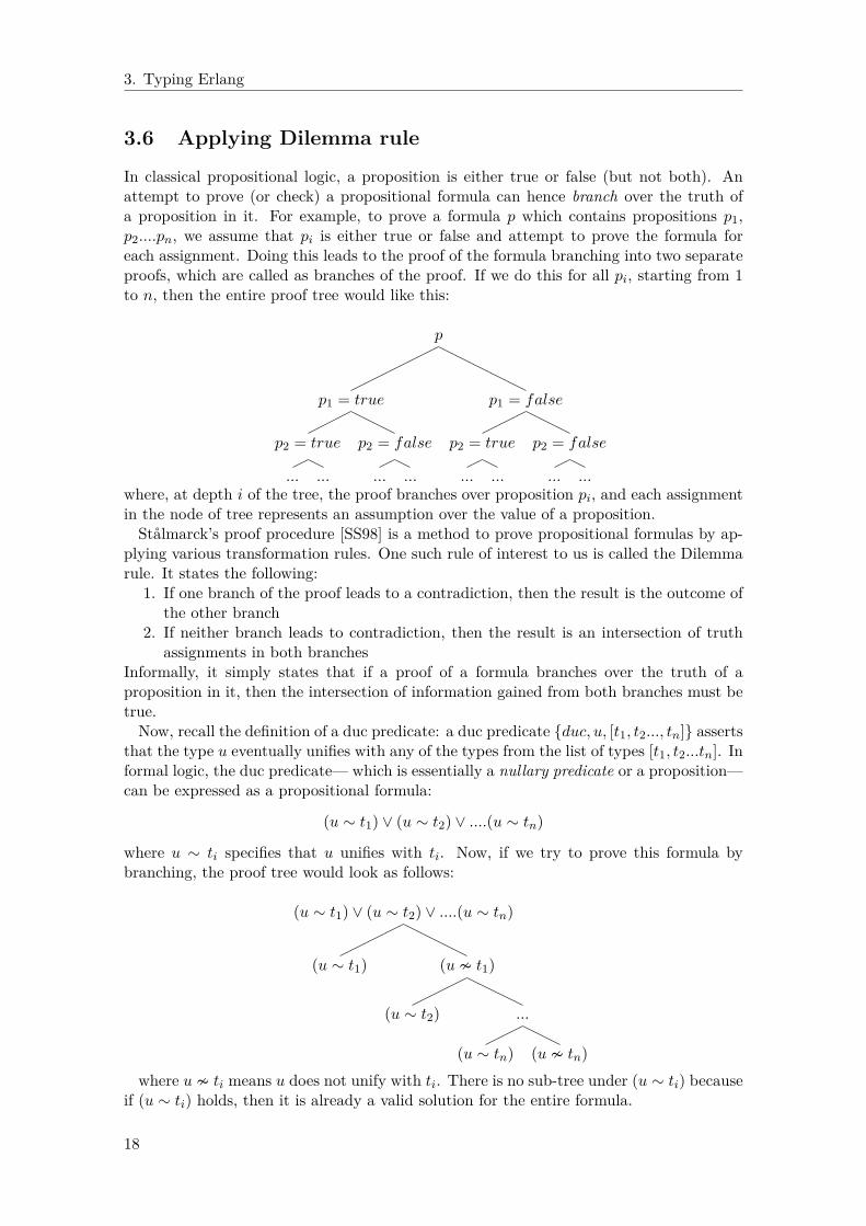
In classical propositional logic, a proposition is either true or false (but not both). Anattempt to prove (or check) a propositional formula can hence branch over the truth ofa proposition in it. For example, to prove a formula p which contains propositions p1,p2....pn, we assume that pi is either true or false and attempt to prove the formula foreach assignment. Doing this leads to the proof of the formula branching into two separateproofs, which are called as branches of the proof. If we do this for all pi, starting from 1to n, then the entire proof tree would like this:

p

p1 = true

p2 = true

... ...

p2 = false

... ...

p1 = false

p2 = true

... ...

p2 = false

... ...where, at depth i of the tree, the proof branches over proposition pi, and each assignmentin the node of tree represents an assumption over the value of a proposition.Stålmarck’s proof procedure [SS98] is a method to prove propositional formulas by ap-

plying various transformation rules. One such rule of interest to us is called the Dilemmarule. It states the following:

1. If one branch of the proof leads to a contradiction, then the result is the outcome ofthe other branch

2. If neither branch leads to contradiction, then the result is an intersection of truthassignments in both branches

Informally, it simply states that if a proof of a formula branches over the truth of aproposition in it, then the intersection of information gained from both branches must betrue.Now, recall the definition of a duc predicate: a duc predicate {duc, u, [t1, t2..., tn]} asserts

that the type u eventually unifies with any of the types from the list of types [t1, t2...tn]. Informal logic, the duc predicate— which is essentially a nullary predicate or a proposition—can be expressed as a propositional formula:

(u ∼ t1) ∨ (u ∼ t2) ∨ ....(u ∼ tn)

where u ∼ ti specifies that u unifies with ti. Now, if we try to prove this formula bybranching, the proof tree would look as follows:

(u ∼ t1) ∨ (u ∼ t2) ∨ ....(u ∼ tn)

(u ∼ t1) (u � t1)

(u ∼ t2) ...

(u ∼ tn) (u � tn)where u � ti means u does not unify with ti. There is no sub-tree under (u ∼ ti) because

if (u ∼ ti) holds, then it is already a valid solution for the entire formula.

18

3. Typing Erlang

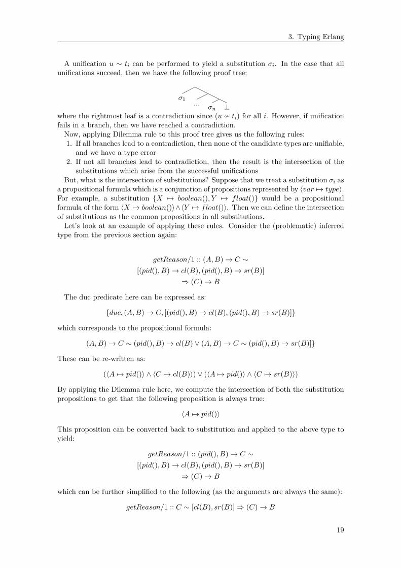
A unification u ∼ ti can be performed to yield a substitution σi. In the case that allunifications succeed, then we have the following proof tree:

σ1 ...σn ⊥

where the rightmost leaf is a contradiction since (u � ti) for all i. However, if unificationfails in a branch, then we have reached a contradiction.Now, applying Dilemma rule to this proof tree gives us the following rules:1. If all branches lead to a contradiction, then none of the candidate types are unifiable,

and we have a type error2. If not all branches lead to contradiction, then the result is the intersection of the

substitutions which arise from the successful unificationsBut, what is the intersection of substitutions? Suppose that we treat a substitution σi as

a propositional formula which is a conjunction of propositions represented by 〈var 7→ type〉.For example, a substitution {X 7→ boolean(), Y 7→ float()} would be a propositionalformula of the form 〈X 7→ boolean()〉∧〈Y 7→ float()〉. Then we can define the intersectionof substitutions as the common propositions in all substitutions.Let’s look at an example of applying these rules. Consider the (problematic) inferred

type from the previous section again:

getReason/1 :: (A,B)→ C ∼[(pid(), B)→ cl(B), (pid(), B)→ sr(B)]

⇒ (C)→ B

The duc predicate here can be expressed as:

{duc, (A,B)→ C, [(pid(), B)→ cl(B), (pid(), B)→ sr(B)]}

which corresponds to the propositional formula:

(A,B)→ C ∼ (pid(), B)→ cl(B) ∨ (A,B)→ C ∼ (pid(), B)→ sr(B)]}

These can be re-written as:

(〈A 7→ pid()〉 ∧ 〈C 7→ cl(B)〉) ∨ (〈A 7→ pid()〉 ∧ 〈C 7→ sr(B)〉)

By applying the Dilemma rule here, we compute the intersection of both the substitutionpropositions to get that the following proposition is always true:

〈A 7→ pid()〉

This proposition can be converted back to substitution and applied to the above type toyield:

getReason/1 :: (pid(), B)→ C ∼[(pid(), B)→ cl(B), (pid(), B)→ sr(B)]

⇒ (C)→ B

which can be further simplified to the following (as the arguments are always the same):

getReason/1 :: C ∼ [cl(B), sr(B)]⇒ (C)→ B

19

3. Typing Erlang

This is the essence of applying the Dilemma rule to extract type information from the ducpredicates.Here, we have illustrated the extraction of type information from a single duc predicate

and the simplification of the inferred type constraint. In the presence of multiple ducpredicates, say d1, d2, ..dn, the propositional formula at the root of the proof tree is aconjunction of all the propositional formulas of the corresponding duc predicates: d1∧d2∧..dn. To solve this formula, we first compute the substitution of d1 to yield a substitutionγ1. This substitution is then applied to d2 and then solved to yield a substitution γ2 andso on until dn . The final resulting substitution is γn ◦ ...γ2 ◦ γ1. The main idea here is tocompose all the substitutions as all the propositions must be true for the formula to betrue.

20

4Partial Evaluation

In this chapter, we discuss the implementation of a simple partial evaluator for Erlang.

4.1 Overview of Partial Evaluation

An evaluation of a function accepts some inputs and produces an output. The requiredinputs must be made available prior to evaluation of the function. Typically, the availabil-ity of all the inputs and the evaluation of the function happens only at runtime. However,one can often find values for some of these inputs at compile time. The availability ofthese inputs can be used to pre-compute parts of the function body at compile time. Thisis the essence of partial evaluation.Consider the following Erlang function which computes the Nth power of a number X:

power(0,_) -> 1;power(N,X) -> X * power(N-1,X).

The variables N and X are the required inputs for this function. The variables whose valuesare available at the time of partial evaluation are called static variables. The variableswhose values are not available until runtime are called dynamic variables. In the functioncall, power(3,2), N and X are both static variables with values N=3 and X=2. Partialevaluation of power(3,2) replaces the function call with its pre-computed value 8.Now, suppose X is dynamic and N is static with value N=3, as in power(3,X). In this

case, we cannot pre-compute the function application as the value of X is not known atthis time. However, we can use the value of N to reduce the application to a simpler form.By definition of the function, we get that power(3,X) equals X * power (3-1 ,X), whichcan be further simplified to X * power (2,X) by constant folding. In a similar fashion,we can reduce power (2,X) until we reach the base case power (0,X), which equals 1.Now by replacing the function applications with their reduced expressions, we get thatpower(3,X) equals X*X*X*1. The resulting expression is called the residual expression.Computing such a residual expression is the goal of partial evaluation.Partial evaluation specializes a program to another program by removing the computa-

tions involving static variables. The resulting specialized program is visibly simpler (forexample, function calls have been removed) and executes faster than the original programsince the static parts have been pre-computed. Partial evaluation’s ability to specializeprograms also has an interesting application in automatic compiler generation. This wasobserved by Futamura in 1971 [Fut71], and hence called the Futamura projections. Inthis thesis, we are interested in exploring a novel idea of applying partial evaluation ofprograms to aid type inference.

21

4. Partial Evaluation

4.2 Partial Evaluation for Erlang

Erlang is a call by value (CBV) language which, unlike a pure language, allows arbitraryside-effects to be performed during execution of a function. A partial evaluator for Erlangmust ensure that CBV semantics is preserved and that side-effects are not re-ordered.Another challenge is Erlang’s pattern matching, which is quite sophisticated and can be

tricky to get right. This section discusses the techniques used to solve these problems.

4.2.1 Setting up the basics

An Erlang program is a list of top level function definitions. As we will see later, weare only interested in partially evaluating some top level functions to aid type inference.Hence, the problem is essentially one of partially evaluating a top level function.A top level function contains a number of function clauses, each of which have a list of

arguments (which might be patterns), guards and a body. A body is a list of expressions.A variable in an expression is bound if it has been defined using pattern matching. Patternmatching can be done using match, case, try expressions or using function arguments. Abound variable may be static or dynamic. It is static if the value it is matched against isknown at specialization time, and dynamic if the value is not known.A core subroutine used by partial evaluation of a top level function is called reduce, and

is implemented by a function reduce/2 which partially evaluates a given expression usingan environment and returns the evaluated expression and a new environment.reduce (Expr ,Env) ->

...{ EvaluatedExpr , UpdatedEnv }

The environment is the state of partial evaluation, which contains things such as variablebindings, seen variables and function definitions. reduce returns the evaluated expressionand a new environment as it may update the environment during partial evaluation (forexample, reducing a match expression P = Q may bring new variable bindings into scope).

4.2.2 Preserving program semantics

The case for variables in reduce/2 is implemented by simply looking up the correspondingexpression bound to the variable in the environment. If the variable has a value in theenvironment (because it’s static), then the value is returned as the reduced expression.Otherwise, the variable is returned as it is (because it’s dynamic).Given this treatment of variables, it is important to ensure that an expression assigned to

a variable in the environment is always a value in order to preserve call by value semantics.To understand the need for it, consider the function expression:fun(Y) ->

X = foo(Y),X + X

end

Here, if we simply assign the function call foo(Y) to X in the environment, then X + Xwould be reduced to foo(Y) + foo(Y) which would end up in foo(Y) being called twice.This not only does not preserve CBV semantics, but might also end up in side-effectsbeing duplicated if foo(Y) does some side-effects.One option is to limit these expressions to static values alone. However, a lot of special-

ization information can be lost in doing so. For example,

22


fun(X) ->Y = XY

end

Here, X is dynamic. Evidently this function can be reduced to the identity function. Butthis cannot be achieved if we limit the expressions assigned to variables in the environmentto static values.A better solution is to treat variables as values. This is because variables are simply

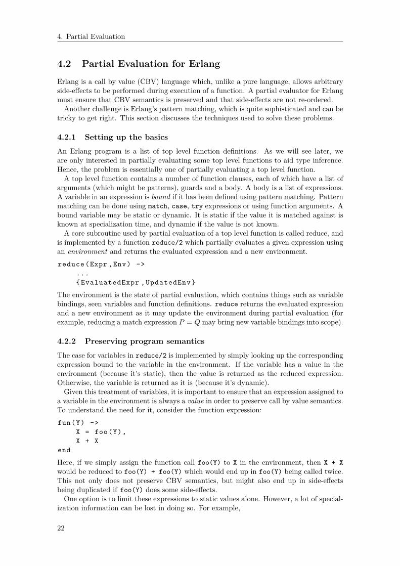
considered as references and duplicating them is harmless. Concretely, an expression isa value if the function isValue/1 returns true for it (implementation for part of whichis shown in figure 4.1). As discussed, the case of variable is defined as true. As a result,expressions such as {X,Y} are treated as values and this leads to much better specialization.Erlang allows the expression which is pattern matched against to contain non-value

expressions such as function calls. One option is to simply retain this expression as it isin the residual program and this would lead to the semantics being preserved. However,we can do much better than that. For example, consider the following function:

fst(A,B) ->X = {id(A),id(B)},case X of

{P,Q} -> Pend.

The expression {id(A),id(B)} returns false for isValue, and hence will not be assignedto X. As a result, this specialized version of this program will be the same as the originalprogram. But is it evident that this function can be reduced to return the value of id(A).To achieve this, we convert the expression {id(A),id(B)} to a value by replacing allfunction calls with variables as follows:

fst(A,B) ->X_1 = id(A),X_2 = id(B),X = {X_1 ,X_2},case X of

{P,Q} -> Pend.

Now, since {X_1,X_2} is a value, this function gets reduced to:

fst(A,B) ->X_1 = id(A),X_2 = id(B),X_1.

This conversion is implemented by a function convertToValue which accepts an expressionas an argument and returns the expression (where all function calls are replaced with freshvariables) and defining bindings for the fresh variables in the expression.

4.2.3 Pattern matching

Pattern matching in performed in Erlang using match (=), case, receive, try or functionarguments. In this section, we discuss partial evaluation of the match expression. The

23


isValue ({ float ,_,_}) -> true;isValue ({ integer ,_,_}) -> true;...isValue ({var ,_,_}) -> true;isValue ({cons ,_,H,T}) -> isValue (H) and isValue (T);isValue ({ tuple ,_,Es}) -> lists:all(fun isValue /1, Es);isValue (_) -> false.

Figure 4.1: Check if an AST node is a value

essence of pattern matching is the same in the other expressions and the implementationis analogous.Consider the match expression P = Q. P is allowed to have unbound variables, and such

variables are considered bound after the match expression. However, Q cannot containany unbound variables. For example, 3 = X is illegal if X is not already bound. Thesemantics of the P = Q is as follows: if the value of P and Q are known, then do aruntime check to ensure that their values are equal. Otherwise, assign the variables in Pto the corresponding values in Q, and vice-versa. The case that unbound variables cannotoccur in Q but variables in Q can be assigned values in P applies because Q can containdynamic variables. Recall that a dynamic variable is a bound variable. For example, theX in the expression foo (X) -> 3 = X, X + 1. is legal and is assigned the value 3 afterthe match expression.A partial evaluator must implement the exact same thing, except with partially available

values: if the value of P is known at specialization time, then assert that it matches Q,otherwise bind variables in P (Q) to the reduced values in Q (P ). To achieve this twoway instantiating of variables, we use unification. Unification, in the context of patternmatching, is very similar to unification in type inference. In type inference, unificationtakes two partially known types that must be equal and instantiates type variables inthem so that it is indeed the case. Instead, in pattern matching, it takes two terms andinstantiates term variables in them. For example, the unification of the terms {X, [Y ]}and {5.0, Z} yields a substitution {X 7→ 5.0, Z 7→ [Y ]}—which are the expected values ofthe corresponding variables in pattern matching.To reduce a match expression P = Q, first we reduce P in the given Env to get a

reduced P ′ and an updated Env′. This is because Erlang allows simple expressions whichcan be computed statically to occur on the left. Then, we reduce Q (in the same Env)to get Q′ and an environment which is discarded (as new variables cannot be bound onthe left). The reduced Q′ is then converted to a value using convertToValue to yieldQ′′. The resulting defining bindings are collected to be returned along with the finalreduced expression. Then, we unify P ′ and Q′′, which—if successful—yields a substitutionσ which maps variables in P ′ to their corresponding expressions in Q′′ and variablesin Q′′ to corresponding expressions in P ′. Note here that unification is more powerfulthan the expected semantics of the match expression in Erlang as the substitution mayalso instantiate an unbound variable on the right. To avoid this, we must ensure thatthe returned substitution only substitutes variables that are recorded as bound in theenvironment.Finally, we update the environment Env′ with the substitution σ (because a substitu-

tion is a list of assignments to a variables) to yield a new environment Env′′—which isthe returned environment. If P ′ is a variable and Q′′ is a value, then the final reduced

24


expression is block of expressions created using the accumulated defining bindings and thevalue Q′′ at the end. Otherwise, the block has P ′ = Q′′ at the end.

4.2.4 Branching

Branching can be done in Erlang using case, if, receive, try and function clauses. Inthis section, we discuss the implementation of reducing a case expression.A case expression consists of an expression E whose value is used for pattern matching

and a list of clauses C1, C2, ..Cn. Each clause contains a pattern Pi, a list of guards Gi

and a clause body Bi (which is a list of expressions). The expected behaviour of a caseexpression is as follows: the body of the first clause, whose pattern matches with E andwhose guards (if any) evaluate to true, is executed. This clause is also called the matchingclause. If no such clause is found, an error is reported.To achieve this semantics in the partial evaluator, we first reduce E to yield a reduced

E′. E′ is then converted to a value, which results in the value E′′ and some definingbindings for the generated fresh variables in E′′. Then, we reduce the clauses to yieldreduced clauses C ′

1, C′2, ..C

′n.

Now, we are ready to do the pattern matching on E′′, and we must chose the first(reduced) matching clause. If no one matching clause can be determined at specializationtime, a new case expression is built using the reduced clauses which may match at runtime.Otherwise, the body of the first matching is returned as the reduced expression.Finding a matching clause happens in two stages: a filter stage and a build stage. The

filter stage performs pattern matching in each clause and uses the result of unification toreduce the clause C ′

i to yield C ′′i . When P ′′

i and E′′ are static values, we can determine ifthe pattern matches: if it does, then we have found a matching clause and filter returnsimmediately. However, if they aren’t static values then we do not have enough informationat the time to decide whether this clause will match and hence we must retain it in theresult of filter. The other case is when the unification of pattern P ′

i E′′ fails, in which

case we may discard C ′′i (since they will never match), and proceeds to the check the next

clause.After this, the build stage packs the resulting clauses from filter into an expression. If

the result is exactly one clause, then the body of the clause is returned as the reducedexpression. However, if it contains multiple clauses, then it means that the reductioncannot decide over one clause. In this case, all the remaining clauses are packed into acase expression—which is returned as the reduced expression.

4.2.5 Function application

A function in Erlang can have multiple clauses. The selection of a function clause to beexecuted in a function call is the same as case: the body of the first matching clause (wherepatterns match the arguments and guards evaluate to true) is executed. The difference,however, is that a function can contain multiple patterns in a clause, while a case cancontain only one.To reduce a function application, first we reduce the arguments. The current implemen-

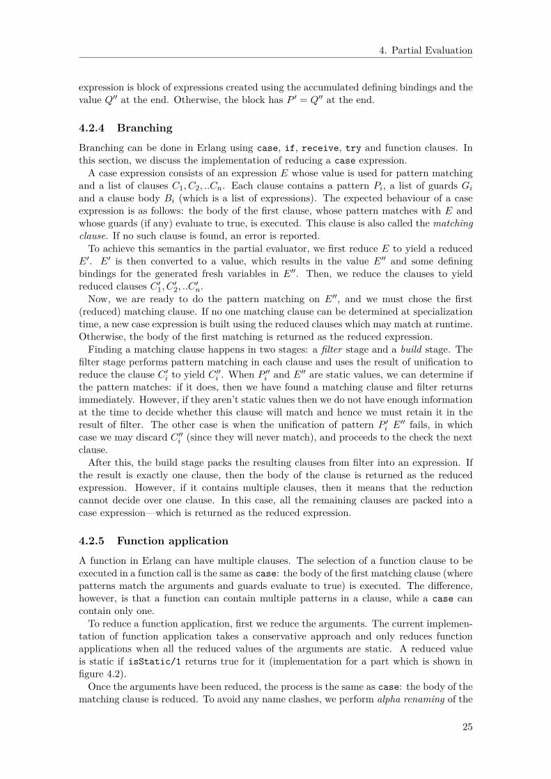
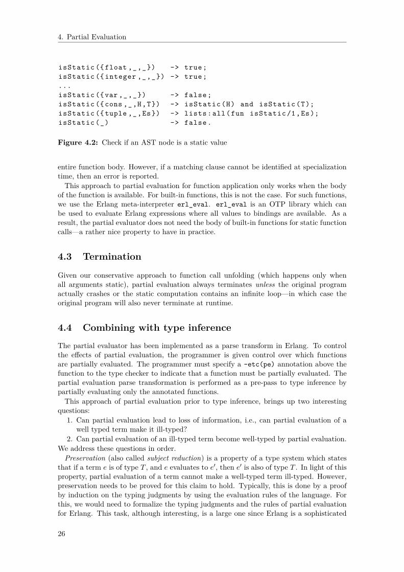
tation of function application takes a conservative approach and only reduces functionapplications when all the reduced values of the arguments are static. A reduced valueis static if isStatic/1 returns true for it (implementation for a part which is shown infigure 4.2).Once the arguments have been reduced, the process is the same as case: the body of the

matching clause is reduced. To avoid any name clashes, we perform alpha renaming of the

25


isStatic ({ float ,_,_}) -> true;isStatic ({ integer ,_,_}) -> true;...isStatic ({var ,_,_}) -> false;isStatic ({cons ,_,H,T}) -> isStatic (H) and isStatic (T);isStatic ({ tuple ,_,Es}) -> lists:all(fun isStatic /1,Es);isStatic (_) -> false.

Figure 4.2: Check if an AST node is a static value

entire function body. However, if a matching clause cannot be identified at specializationtime, then an error is reported.This approach to partial evaluation for function application only works when the body

of the function is available. For built-in functions, this is not the case. For such functions,we use the Erlang meta-interpreter erl_eval. erl_eval is an OTP library which canbe used to evaluate Erlang expressions where all values to bindings are available. As aresult, the partial evaluator does not need the body of built-in functions for static functioncalls—a rather nice property to have in practice.

4.3 Termination

Given our conservative approach to function call unfolding (which happens only whenall arguments static), partial evaluation always terminates unless the original programactually crashes or the static computation contains an infinite loop—in which case theoriginal program will also never terminate at runtime.

4.4 Combining with type inference

The partial evaluator has been implemented as a parse transform in Erlang. To controlthe effects of partial evaluation, the programmer is given control over which functionsare partially evaluated. The programmer must specify a -etc(pe) annotation above thefunction to the type checker to indicate that a function must be partially evaluated. Thepartial evaluation parse transformation is performed as a pre-pass to type inference bypartially evaluating only the annotated functions.This approach of partial evaluation prior to type inference, brings up two interesting

questions:1. Can partial evaluation lead to loss of information, i.e., can partial evaluation of a

well typed term make it ill-typed?2. Can partial evaluation of an ill-typed term become well-typed by partial evaluation.

We address these questions in order.Preservation (also called subject reduction) is a property of a type system which states

that if a term e is of type T , and e evaluates to e′, then e′ is also of type T . In light of thisproperty, partial evaluation of a term cannot make a well-typed term ill-typed. However,preservation needs to be proved for this claim to hold. Typically, this is done by a proofby induction on the typing judgments by using the evaluation rules of the language. Forthis, we would need to formalize the typing judgments and the rules of partial evaluationfor Erlang. This task, although interesting, is a large one since Erlang is a sophisticated

26


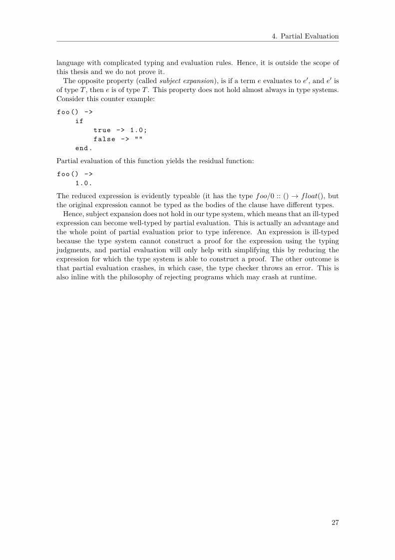
language with complicated typing and evaluation rules. Hence, it is outside the scope ofthis thesis and we do not prove it.The opposite property (called subject expansion), is if a term e evaluates to e′, and e′ is

of type T , then e is of type T . This property does not hold almost always in type systems.Consider this counter example:

foo () ->if

true -> 1.0;false -> ""

end.

Partial evaluation of this function yields the residual function:

foo () ->1.0.

The reduced expression is evidently typeable (it has the type foo/0 :: () → float(), butthe original expression cannot be typed as the bodies of the clause have different types.Hence, subject expansion does not hold in our type system, which means that an ill-typed

expression can become well-typed by partial evaluation. This is actually an advantage andthe whole point of partial evaluation prior to type inference. An expression is ill-typedbecause the type system cannot construct a proof for the expression using the typingjudgments, and partial evaluation will only help with simplifying this by reducing theexpression for which the type system is able to construct a proof. The other outcome isthat partial evaluation crashes, in which case, the type checker throws an error. This isalso inline with the philosophy of rejecting programs which may crash at runtime.

27


28

5Results

Evaluating a type checker is a tricky problem. One way to do this is by running it againstvarious libraries. However, applying our type checker to popular Erlang/OTP librariesdemands a much larger coverage of the language. For example, most Erlang programs usefeatures such as remote function calls (functions defined in other modules), records anderror handling. These features have not been implemented yet.

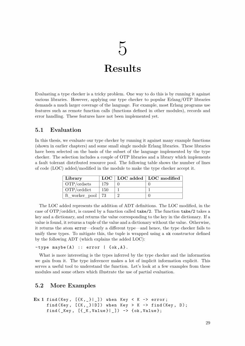
5.1 EvaluationIn this thesis, we evaluate our type checker by running it against many example functions(shown in earlier chapters) and some small single module Erlang libraries. These librarieshave been selected on the basis of the subset of the language implemented by the typechecker. The selection includes a couple of OTP libraries and a library which implementsa fault tolerant distributed resource pool. The following table shows the number of linesof code (LOC) added/modified in the module to make the type checker accept it.

Library LOC LOC added LOC modifiedOTP/ordsets 179 0 0OTP/orddict 150 1 1ft_worker_pool 73 2 0

The LOC added represents the addition of ADT definitions. The LOC modified, in thecase of OTP/orddict, is caused by a function called take/2. The function take/2 takes akey and a dictionary, and returns the value corresponding to the key in the dictionary. If avalue is found, it returns a tuple of the value and a dictionary without the value. Otherwise,it returns the atom error—clearly a different type—and hence, the type checker fails tounify these types. To mitigate this, the tuple is wrapped using a ok constructor definedby the following ADT (which explains the added LOC):

-type maybe(A) :: error | {ok ,A}.

What is more interesting is the types inferred by the type checker and the informationwe gain from it. The type inferencer makes a lot of implicit information explicit. Thisserves a useful tool to understand the function. Let’s look at a few examples from thesemodules and some others which illustrate the use of partial evaluation.

5.2 More Examples

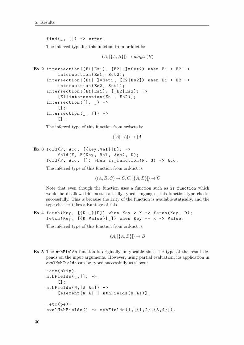
Ex 1 find(Key , [{K,_}|_]) when Key < K -> error;find(Key , [{K,_}|D]) when Key > K -> find(Key , D);find(_Key , [{_K ,Value }|_]) -> {ok ,Value };

29

5. Results

find(_, []) -> error.

The inferred type for this function from orddict is:

(A, [{A,B}])→ maybe(B)

Ex 2 intersection ([E1|Es1], [E2|_]= Set2) when E1 < E2 ->intersection (Es1 , Set2 );

intersection ([E1|_]=Set1 , [E2|Es2 ]) when E1 > E2 ->intersection (Es2 , Set1 );

intersection ([E1|Es1], [_E2|Es2 ]) ->[E1| intersection (Es1 , Es2 )];

intersection ([], _) ->[];

intersection (_, []) ->[].

The inferred type of this function from ordsets is:

([A], [A])→ [A]

Ex 3 fold(F, Acc , [{Key ,Val }|D]) ->fold(F, F(Key , Val , Acc), D);

fold(F, Acc , []) when is_function (F, 3) -> Acc.

The inferred type of this function from orddict is:

((A,B,C)→ C,C, [{A,B}])→ C

Note that even though the function uses a function such as is_function whichwould be disallowed in most statically typed languages, this function type checkssuccessfully. This is because the arity of the function is available statically, and thetype checker takes advantage of this.

Ex 4 fetch(Key , [{K,_}|D]) when Key > K -> fetch(Key , D);fetch(Key , [{K,Value }|_]) when Key == K -> Value.

The inferred type of this function from orddict is:

(A, [{A,B}])→ B

Ex 5 The nthFields function is originally untypeable since the type of the result de-pends on the input arguments. However, using partial evaluation, its application inevalNthFields can be typed successfully as shown:

-etc(skip ).nthFields (_ ,[]) ->

[];nthFields (N,[A|As]) ->

[ element (N,A) | nthFields (N,As )].

-etc(pe).evalNthFields () -> nthFields (1 ,[{1 ,2} ,{3 ,4}]).

30

5. Results

The inferred type of the latter function is:

evalNthFields/0 :: Num D ⇒ ()→ [D]

Ex 6 The following function replaces a cons constructor by a two-tuple, and a nil by anempty tuple. The original application (as in the previous example) is untypeable.However, we can type its application when the arguments are available:

-etc(skip ).tuplize ([]) ->

{};tuplize ([X|Xs]) ->

{X, tuplize (Xs )}.

-etc(pe).evalTuplize () -> tuplize ([1 ,2 ,3]).

The inferred type is:

evalTuplize/0 :: (Num E,Num F,Num G)⇒ ()→ {E, {F, {G, {}}}}

Ex 7 This example demonstrates that partial evaluation is not limited to static values.

-etc(pe).foo(F,G,X) ->

T = {F(X),G(X)},element (1,T).

In spite of F, G and X being dynamic variables, the inferred type of this function is:

foo/3 :: ((A)→ B, (A)→ C,A)→ B

This is because the structure of T to determine that that the return type must bethe type of F(X).

31

5. Results

32

6Discussion

6.1 Missing featuresThe current implementation is far from complete and there are many more features whichare required to type large Erlang programs. Most importantly, this includes modules,records and error handling.Currently, remote function calls (calls to functions in other modules) are handled as

follows: the type checker creates a module interface for a module which has been typechecked successfully, and when a remote function call is encountered, it reads the interfacefile if it exists and gets the type from it. However, if it does not exist, it simply spawnsa fresh set of type variables for the function and its arguments—creating an avenue foruncaught type errors. This is more of an in-place mechanism rather than a solution totype checking remote function calls. Given this simple approach, it also does not handlemodule level dependencies.

6.2 LimitationsThe main limitation of the current system is that it does not type check concurrency.Although it does not omit it, the current approach is very simplistic and can lead touncaught type errors. For example, consider this program:

foo () ->receive

X -> Xend.

baz () ->foo () + 1.0.

This program type checks successfully. This is because foo is assigned the type () → A.Evidently, this need not be the case, and if foo receives a non-numeric type, this programcrashes at baz.

6.3 Future work

6.3.1 Records

Records can be typed by generating an ADT for them. For example, for the followingrecord

-record (person ,{name :: [char ()],

33

6. Discussion

age :: integer (),id

}).

we could generate the following ADT:

-type person (A) ::{person ,[ char ()], integer (),A}

The ADT has a single constructor where the arguments to the constructors are the typesof the fields. When the type of a field is not defined, it is parametrized over the type of theADT. In this fashion, a record field access can simply return the type of the constructorargument corresponding to the field.A record update, on the other hand, returns a new record by changing the value of one

or more fields in the original record. If the type of a field has been specified in the recorddefinition, then updated value must be of the same type as the specified type. Otherwise,the updated value maybe of a different type. For example, consider the following recordupdate:

updateId (Rec ,ID) ->Rec# person {id=ID}

Here ID may be of a different type from that of Rec#person.id. Since we want to allowthe change in type of the value, we can assign this function the type

updateId/2 :: (person(A), B)→ person(B)

6.3.2 Concurrency

The most interesting next step would be to type check concurrency. For typing concurrencyin Erlang, an idea which has been "around for a while" is adding effects to the type system[MW97] [Hug02] and typing the pid of the process which receives a message of a certaintype, say float(), as pid(float()). Given that the pid is used to send messages, if the typeof a value received by a process can be captured in the type of its pid, the type system canensure that only messages of the expected type are sent. The types would look as follows:

spawn/1 :: (()→ τ receivesα)→ pid(α)(!) :: (pid(α), α)→ α

where, an expression e with value of type τ and a receive statement for messages of thetype α is of the type τ receives α. spawn/1 is a function which, when called with afunction as an argument, spawns a process and returns the pid. When a function of type() → e receivesα is spawned, it returns a pid of type pid(α). The send operation ! isassigned a type that ensures only messages of type α are sent to a process identified by apid of type pid(α).

6.3.3 Partial Evaluation

The current partial evaluator is very simple and far from complete. It does not specializefunctions where only some of the arguments are available statically. These are in fact themost interesting cases and would lead to much better residual code. For example, thereduction of power(3,X) to X*X*X*1 (discussed earlier) is an example of this because onlyone of the arguments are static. The partial evaluator also needs to be implemented formore parts of the language such as higher order functions and records.

34

6. Discussion

Currently, although partial evaluation strives to not re-order or duplicate side-effects,the preservation of semantics requires a more thorough analysis. The behaviour in thepresence of concurrency has not been tested, and is also an avenue for further work. Partialevaluation of concurrent programs is a challenging problem and appears to have very littleliterature which is directly applicable for Erlang.

6.3.4 Integrating Partial Evaluation and Type Inference

Another avenue for exploration is better integration of the partial evaluator and the typechecker. Currently, partial evaluation is simply a pre-pass to type checking, and thisapproach fails to take advantage of information in one stage in the other. For example,consider the following program

foo(Z) ->[{A,B}|[X|Xs]] = Z,element (2,X)

Type inference knows that X is of the same type as {A,B}, but partial evaluation does notknow that, and hence it does not reduce element(2,X) further.It might be possible to engineer the integration in more interesting ways. One way is to

use partial evaluation as a sub-routine in type inference and call it when a term cannotbe typed. This way, the partial evaluator can be supplied with information from typeinference. This approach may also avoid the need for annotations. A more closely coupledapproach is type specialization [Hug96], which achieves much better exploitation of staticinformation. However, this is a completely different line of work, and this thesis takesa more modular approach to this problem by developing the type inferencer and partialevaluator separately.

6.4 ConclusionIn this thesis, most notably, we develop ways to type overloaded constructors in a Hindley-Milner type system and also illustrate the novel idea of applying partial evaluation to aidtype inference. Overall, the results to type Erlang look promising. The inferred types arevery informative and appear to expose a lot of the program structure. Partial evaluationalso appears to be a suitable to choice to allow some restricted form of flexibility that isenjoyed by Erlang programmers.

35

6. Discussion

36

Bibliography

[DM82] Luis Damas and Robin Milner. Principal type-schemes for functional programs.In Proceedings of the 9th ACM SIGPLAN-SIGACT symposium on Principlesof programming languages, pages 207–212. ACM, 1982.

[Fut71] Yoshihiko Futamura. Partial evaluation of computation process an approachto a compiler-compiler. Systems, computers, controls, 2(5):45–50, 1971.

[Hug96] John Hughes. Type specialisation for the λ-calculus; or, a new paradigm forpartial evaluation based on type inference. In Partial Evaluation, pages 183–215. Springer, 1996.

[Hug02] John Hughes. Typing erlang, 2002.

[JGS93] Neil D Jones, Carsten K Gomard, and Peter Sestoft. Partial evaluation andautomatic program generation. Peter Sestoft, 1993.

[Jon99] Mark P Jones. Typing haskell in haskell. In Haskell workshop, volume 7, 1999.

[LS05] Tobias Lindahl and Konstantinos Sagonas. Typer: a type annotator of erlangcode. In Proceedings of the 2005 ACM SIGPLAN workshop on Erlang, pages17–25. ACM, 2005.

[LS06] Tobias Lindahl and Konstantinos Sagonas. Practical type inference based onsuccess typings. In Proceedings of the 8th ACM SIGPLAN international con-ference on Principles and practice of declarative programming, pages 167–178.ACM, 2006.

[MW97] Simon Marlow and Philip Wadler. A practical subtyping system for erlang.ACM SIGPLAN Notices, 32(8):136–149, 1997.

[Rém02] Didier Rémy. Using, understanding, and unraveling the ocaml language frompractice to theory and vice versa. In Applied Semantics, pages 413–536.Springer, 2002.

[RPFD14] Baishakhi Ray, Daryl Posnett, Vladimir Filkov, and Premkumar Devanbu. Alarge scale study of programming languages and code quality in github. In Pro-ceedings of the 22nd ACM SIGSOFT International Symposium on Foundationsof Software Engineering, pages 155–165. ACM, 2014.

[SS98] Mary Sheeran and Gunnar Stålmarck. A tutorial on stålmarck’s proof proce-dure for propositional logic. In International Conference on Formal Methodsin Computer-Aided Design, pages 82–99. Springer, 1998.

37

Bibliography

38

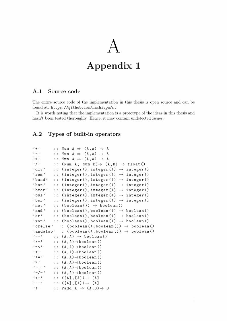
AAppendix 1

A.1 Source code

The entire source code of the implementation in this thesis is open source and can befound at: https://github.com/nachivpn/mtIt is worth noting that the implementation is a prototype of the ideas in this thesis and

hasn’t been tested thoroughly. Hence, it may contain undetected issues.

A.2 Types of built-in operators

’+’ :: Num A ⇒ (A,A) → A’-’ :: Num A ⇒ (A,A) → A’*’ :: Num A ⇒ (A,A) → A’/’ :: (Num A, Num B)⇒ (A,B) → float ()’div ’ :: ( integer (), integer ()) → integer ()’rem ’ :: ( integer (), integer ()) → integer ()’band ’ :: ( integer (), integer ()) → integer ()’bor ’ :: ( integer (), integer ()) → integer ()’bxor ’ :: ( integer (), integer ()) → integer ()’bsl ’ :: ( integer (), integer ()) → integer ()’bsr ’ :: ( integer (), integer ()) → integer ()’not ’ :: ( boolean ()) → boolean ()’and ’ :: ( boolean (), boolean ()) → boolean ()’or ’ :: ( boolean (), boolean ()) → boolean ()’xor ’ :: ( boolean (), boolean ()) → boolean ()’orelse ’ :: ( boolean (), boolean ()) → boolean ()’andalso ’ :: ( boolean (), boolean ()) → boolean ()’==’ :: (A,A) → boolean ()’/=’ :: (A,A)→boolean ()’=<’ :: (A,A)→boolean ()’<’ :: (A,A)→boolean ()’>=’ :: (A,A)→boolean ()’>’ :: (A,A)→boolean ()’=:=’ :: (A,A)→boolean ()’=/=’ :: (A,A)→boolean ()’++’ :: ([A],[A])→ [A]’--’ :: ([A],[A])→ [A]’!’ :: Padd A ⇒ (A,B)→ B

I

https://github.com/nachivpn/mt

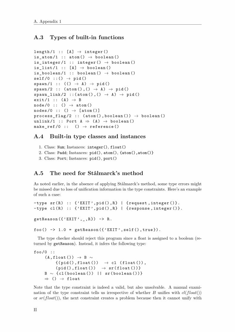
A. Appendix 1

A.3 Types of built-in functions

length /1 :: [A] → integer ()is_atom /1 :: atom () → boolean ()is_integer /1 :: integer () → boolean ()is_list /1 :: [A] → boolean ()is_boolean /1 :: boolean () → boolean ()self /0 ::() → pid ()spawn /1 :: (() → A) → pid ()spawn /2 :: (atom () ,() → A) → pid ()spawn_link /2 ::( atom () ,() → A) → pid ()exit /1 :: (A) → Bnode /0 :: () → atom ()nodes /0 :: () → [atom ()]process_flag /2 :: (atom (), boolean ()) → boolean ()unlink /1 :: Port A ⇒ (A) → boolean ()make_ref /0 :: () → reference ()

A.4 Built-in type classes and instances

1. Class: Num; Instances: integer(), float()2. Class: Padd; Instances: pid(), atom(), {atom(),atom()}3. Class: Port; Instances: pid(), port()

A.5 The need for Stålmarck’s method

As noted earlier, in the absence of applying Stålmarck’s method, some type errors mightbe missed due to loss of unification information in the type constraints. Here’s an exampleof such a case:

-type sr(R) :: {’EXIT ’,pid (),R} | {request , integer ()}.-type cl(R) :: {’EXIT ’,pid (),R} | {response , integer ()}.

getReason ({’EXIT ’,_,R}) -> R.

foo () -> 1.0 = getReason ({’EXIT ’,self (), true }).

The type checker should reject this program since a float is assigned to a boolean (re-turned by getReason). Instead, it infers the following type:

foo /0 ::(A,float ()) → B ∼

{( pid (), float ()) → cl (float ()),(pid (), float ()) → sr(float ())}

B ∼ {cl( boolean ()) || sr( boolean ())}⇒ () → float

Note that the type constraint is indeed a valid, but also unsolvable. A manual exami-nation of the type constraint tells us irrespective of whether B unifies with cl(float())or sr(float()), the next constraint creates a problem because then it cannot unify with

II

A. Appendix 1

cl(boolean()) or sr(boolean(). Applying Stålmarck’s method helps us extract this infor-mation from the type constraints to reject this program as all branches of the proof treewould lead to a contradiction.

A.6 Type errors1. Ensuring all function clauses return the same type:

1. foo4 () -> 3.0 ;2. foo4 () -> "hello ".

...> c(test ).test.erl: error in parse transform ’etc ’:{" Type Error: Cannot unify{bt ,1, float} with {bt ,2, string }" ,..

2. Ensuring a when clause is boolean:

41. foo5 (N) when 1.0 -> true.

...> c(test ).test.erl: error in parse transform ’etc ’:{" Type Error: Cannot unify{bt ,41, float} with {bt ,41, boolean }" ,..

3. Mixing integer and float values:

269. float3 () -> (1.0 + 2.0).270. integer3 () -> 3 div 1.271. heter_add () -> ( float3 () + integer3 ()).

...> c(test ).test.erl: error in parse transform ’etc ’:{" Type Error: Cannot unify{bt ,269 , float} with {bt ,270 , integer }" ,..

4. Mixing numeric with non-numeric values:

82. foo8 () -> 1;83. foo8 () -> "Hello ".

...> c(test ).test.erl: error in parse transform ’etc ’:{" Type Error: Cannot solve predicate :{class ," Num ",{bt ,83, string }}",

III

typing the untypeable in erlang

Documents