NASA Technical Memorandum 107566

/,u-5_7 _-

/-F

SYSTEM/OBSERVER/CONTROLLERIDENTIFICATION TOOLBOX

Jer-Nan Juang, Lucas G. Horta, and Minh Phan

February 1992

N/_ANational Aeronautics andSpace Administration

Langley Research CenterHampton, Virginia 23665

(NASA-TM-I07566) SYSTEM/OBSERVER/CONTROLLER

IDENTIFICATION TOOLBOX (NASA) 87 pCSCL 20K

G3139

N92-2_706

Uncl as

0088785

https://ntrs.nasa.gov/search.jsp?R=19920015463 2018-07-08T21:39:14+00:00Z

r

ACKNOWLEDGEMENT

This is considered as the second version of the original version entitled "System/ObserverRealization Toolbox" which was published in July, 1991 and presented at the short course

taught by the first author in NASA Langley Research Center, Hampton, Virginia. Sincethen, we have doubled the number of function files to include the closed-loopidentification and backward observer identification. The closed-loop identification allowsone to identify not only the open-loop system but also the feedback gain and the effectiveobserver gain. The backward observer identification allows one to smooth the currentmeasurement data from future data. Some of the original function files were completelyrewritten to improve the computational speed and reduce the storage memory. In

particular, the era function files were completely overhauled.

All the function files were written by the authors who developed the system identificationmethods shown in this toolbox, including the Eigensystem Realization Algorithm (ERA),the ERA using Data Correlation (ERA/DC), the Observer/Kalman Filter Identification(OKID), and the Observer/Controller Identification (OCID) and the Backward ObserverIdentification (BOLD). However, this toolbox will not come true without the followingco-developers of the methods mentioned above.

Richard S. Pappa (ERA), NASA Langley Research Center, USA

Jonathan E. Cooper (ERA/DC), University of Manchester, England

Jan R. Wright (ERA/DC), University of Manchester, England

Richard W. Longman (OKID), Columbia University, USA

Chung-Wen Chen (OKID), North Carolina University, North Carolina, USA

Dr. Jiann-shiun Lew who helped write the functions monera, peradc and svra in the

original version is also deeply appreciated.

It takes time to develop a system identification technique useful for structural dynamicsand control testing. We probably would not have been able to develop any usefultechnique had we not had a considerable strong support from our superiors. We thankBrantley R. Hanks and Larry D. Pinson for providing inspiring workingconditions and making our laboratory experience possible in control and systemidentification of flexible space structures.

INTRODUCTION

System identification is the process of constructing a mathematical model from input and output

data for a system under testing, and characterizing the system uncertainties and measurement

noises. The mathematical model structure can take various forms depending upon the intended

use. The SYSTEM/OBSERVER/CONTROLLER IDENTIFICATION TOOLBOX (SOCIT) is a

collection of functions, written in MATLAB I language and expressed in M-files, that implements

a variety of modern system identification techniques. For an open-loop system, the central

features of the SOCIT are functions for identification of a system model and its corresponding

forward and backward observers directly from input and output data. The system and its

observers are represented by a discrete model. The identified model and observers may be used

for controller design of linear systems as well as identification of modal parameters such as

dampings, frequencies, and mode shapes. For a closed-loop system, the central features of the

SOCIT include identification of an open-loop model, an observer and its corresponding

controller gain directly from input and output data. The basic package is capable of:

1- Identifying system, forward and backward observer Markov parameters (pulse responses)

from input and output time histories.

2- Constructing a state space model from pulse responses.

3- Identifying a state space model and its corresponding forward and backward observer gains

directly from input and output time histories.

4- Identifying a forward observer/Kalman filter gain with a given state space model, and input

and output time histories.

5- Computing variance and bias for identified modal parameters using Monte Carlo and

perturbation procedures.

6- Computing forward prediction errors and backward smoothing errors for any of the models

generated.

7- Identifying a state space model, and its corresponding controller gain and observer/Kalman

filter gain directly from input, output and control force time histories.

The unique features of this package are:

1- No nonlinear programming involved.

2- No a priori noise information required.

3- Guided model order selection.

4- Direct identification of system & observer/Kalman filter.

5- Direct identification of closed-loop controller.

6- Suitable for stable & unstable systems.

1 © Copyright 1985-91, by Mathworks, Inc. All rights reserved

Notes .....

2

SYSTEM�OBSERVER�CONTROLLERIDENTIFICATION TOOLBOX

Reference

Page

arx barx-bat

m

arxc

arx fb

arx_psbk_diagblock tr

cpulseera

eradc

freq_pthanklhankldc

k abcd

m2p

mar com

mar oc

mar_sepmar_yoc

matchmodal

monera

ocid

- calculates backward observer Markov parameters and residual error ......... 11

- calculates observer Markov parameters and prediction error ................... 11

- computes the combined observer/controller Markov parametersfrom feedback control input and output data ...................................... 14

- calculates forward and backward observer Markov parameters,and their residual errors ............................................................. 11

- calculates observer Markov parameters from pulse response samples ......... 16

- transforms the modal form into a real block diagonal form .................... 18

-computes matrix block transposition .............................................. 20

- converts rich input responses to pulse response time histories ................ 21

identifies a state space model from pulse response time historiesusing system realization theory (ERA) ............................................ 23

- identifies a state space model from pulse response time historiesusing a data correlation technique (ERA/DC) .................................... 23

- plots the transfer function representation of a discrete time system ............ 27

-forms a Hankel matrix from Markov parameters ................................. 29

- forms a data correlation matrix for eradc .......................................... 30

- identifies an Observer filter gain matrix from test data for a knowndiscrete system model to whiten the stochastic residual ........................ 31

- rearranges a Markov parameters sequence in the form of pulseresponse samples .................................................................... 33

- computes a specified number of system Markov parameters fromobserver Markov parameters. 34

- computes a specified number of system, observer, and controllerMarkov parameters from observer/controller Markov parameters ............. 36

- equivalent to mar_corn but with separate observer Makov parameters ........ 34

- computes a specified number of system, observer, and controllerMarkov parameters from feedback control inputs and outputs ................. 38

- matches the eigenvalues identified from forward and backward models ...... 40

- computes a reduced stable or unstable model in modal coordinates ........... 42

- calculates variance of ERA identified parameters using the MonteCarlo approach ...................................................................... 43

- identifies a state space model, an observer gain, and a controllergain from closed-loop experimental data ......................................... 45

3

okid

okid b

okid fb

okid_pp2m

peradc

pred_err

pred_efb

pred erbpulse-ryucovar

separatesvpm

svra

uy_stack

y_closed

y_esti

y_pred

yucovar

yucovfb

byucov_

yycovar

- identifies simultaneously a state space model and an observer gainfrom input and output data .......................................................... 50

- modified version of okid using a backward observer ........................... 50

- combined version of okid and okid_b using forward and backwardobservers .............................................................................. 50

- identifies a state space model from pulse response samples ................... 50

- rearranges pulse response samples in the form of Markov parameterssequence ............................................................................. 62

- c',dculates the variance and bias of ERA/DC identified parametersfor single input and single output systems ....................................... 63

- computes prediction error from estimated observer Markovparameters ............................................................................ 65

- computes prediction and smoothing errors from estimatedforward and backward observer Markov parameters ........................... 65

- computes smoothing errors from estimated backward parameters ............. 65

- computes pulse response samples from general input and output data ......... 67

- computes the left correlation matrix associated with the feedbackcontrol input for an observer/controller identification ............................ 69

- separates a given matrix sequence into two sequences ........................... 71

- calcalates modal observability matrix and the singular valuecontribution of each mode to the pulse response samples ....................... 72

- identifies a state space model from input and output data using astate vector realization technique .............................................. 74

- computes a stacked matrix with inputs and outputs .............................. 76

- reconstructs closed-loop response time histories using ocididentified system, observer, and controller gain matrices ...................... 77

- reconstructs outputs using an identified observer ................................ 78

- reconstructs outputs using an identified system model .......................... 79

- computes auto-correlation and cross-correlation matrices betweeninputs and outputs ................................................................... 80

- computes forward and backward auto-correlation and cross-correlation matrices between inputs and outputs ................................. 80

- computes backward auto-correlation and cross-correlation matricesbetween inputs and outputs ........................................................ 80

- computes the left and right output residual correlation matrix .................. 83

4

Road Map for Identification of anOpen-Loop System(general input/output data)

okid bokid_-fb

Input and Output Time Histories

r-"

I

I

I

I

I

arx b Iarx-fb arx_bat

Observer MarkovParameters

mar_corn

okid _ 1

System MarkovParameters

_ m2p _

Observer GainMarkov Parameters

L

era eradc

_r

System Matrices A, B, C, DObserver Gain Matrix G

1

I

I

I

I

I

I

I

I

I

I

I

I

I

I

I

I

I

I

I_J

Note that Markov parameters also mean pulse response time histories.

5

Road Map for Identification of anOpen-Loop System

(pulse response time histories)

okid_p

Pulse Response Time Histories

t arx_ps

Observer MarkovParameters

mar_sep

System MarkovParameters

Observer GainMarkov Parameters

m2p

era eradc

1

I

I

I

I

!

I

I

I

I

I

I

I

I

I

I

I

I

I

/

System Matrices A, B, C, DObserver Gain Matrix G

Note that Markov parameters also mean pulse response time histories.

6

Road Map for Identification of aClosed-Loop System(general input/output data)

Input, Output and Control ForceTime Histories

l arxc

ocid

L

System Markov

Observer/Controller

Markov Parameters

mar_oc _ mar_yoc

Parameters Observer Gain ]Markov Parameters

m2p

era

• "l'Controller Gain IMarkov Parameters I

eradc

J

System Matrices A, B, C, DObserver Gain Matrix G

Controller Gain F

Note that Markov parameters also mean pulse response time histories.

7

am

0

a

rd

0

IXI

_zF- _n_ O_

8

0

m

c0 O_ 0

Ill

IIm

1,1,,,,iim

9

Notes

10

arx_b,arx_bat,arx_fbPurpose:

Compute observer Markov parameters.

Synopsis:

l Ybf]=arx_b(m,r,u,y,p,icl)[Yf]=arx-bat(m,r,u,y,p ,ic2 )[Yf ,Yb ]=arx_fb(m,r,u,y,p ,ic2 )

Description:

The function computes observer Markov parameters from input/output data. The identified

observer system is deadbeat oforderp. Given I samples, r inputs, and m outputs, the inputmatrix u must have dimensions I x r and output y l × m. Multiple experiments may beused in these functions. In that case, the input matrix u becomes I x (rn,) where n, is thenumber of experiments, and the output matrix becomes I x (ran,). Function arx_bat solvesthe least squares problem of a forward observer;

where

y/= [y(0)y(1)...y(l - 1)l

Y/ = ID C-B CA-B ... C-A _'-'-B I

u(0) u(1) u(2)..- u(/-1)

v_ = v(0) v(l) ... v(t- 2):

v(O) ... v(l- p- 1)

_r,,,,1v(i) Ly(i)j, i = 0,1 ..... l- 1

Here "A= A + GC, -B = [B + GD -G], in which A, B, C, D are system matrices, and G isthe forward observer gain matrix. See function okid for more discussion on the definition

of these matrices. The solution is stored in Yf of dimension m ×[(r+ m)p + r] If the

experiment started from rest ic2(1)=O, otherwise, ic2(1)=l. Once an estimate of the

parameters is available the user is given the option to compute the prediction error

eI =Y_.I-Yyl

This computation when analyzing long records is time consuming. The square root of thediagonal elements of the inverse correlation matrix are proportional to the parametervariance. A chart depicting these values is plotted along with the prediction error. To bypassthe prediction error option, set the second element of ic2 to one, i.e. ic2(2)=0.

Function arx_b solves the least squares problem of a backward observer as follows

11

y_ = _V_where

Yb = [y(0)y(1)---y(l - p - 2)]

u(0) u(1) u(2) ... u(l-p-2) 1

v_= v(,p.) v(p + 1) v(p_+2) --- v(li- 2) /!

L v(l) v(2) v(3) ... v(l- p - 1)J

v(i)=i.y(i)j; /=o,1....,t-I

Here, ,4 = A -1 + GC, /} =-A-IB, in which A, B, C, D are system matrices, and G is the

backward observer matrix. See function okid_b for more discussion on the definition of

these matrices. The solution is stored in Yb of dimension m x [(r +m)p + r]. Once an

estimate of the parameters is available the user is given the option to compute the smoothingerror, instead of the prediction error as in the case for the forward observer.

eb = Yb -- YbVb

The square root of the diagonal elements of the inverse correlation matrix are proportional to

the parameter variance. A chart depicting these values is plotted along with the smoothingerror. To bypass the smoothing error opuon, set the the variable ic to one, i.e. icl=O. Notethat icl is a scalar whereas ic2 is a vector with two elements.

Observation. of the forward and backward formulations shown above immediately reals that

one may simultaneously compute forward and backward observer parameters. Bothmatrices are very similar in the sense that their lower sides are identical. Function arx_fbsolves for backward and forward observer parameters simultaneously. All parameters used

above also apply to this function.

Algorithm:

First, the correlation matrices are computed without actually constructing the individual

matrices. The parameter estimate is obtained by

Y = yV r (VV r)+

where (+) refers to pseudo inverse. The pseudo inverse is computed using singular value

decomposition.

12

Example:

r=l ;m=l ;ic=[0 11;index---0;p=2;L=100;a=[0 -0.16; 1 -ll; b=10 1]'; c=[0 1]; d:0; G=[0.16 1]';

u--rand(L,m);

y--dlsim(a,b,c,d,u);psize--r+p*(r+m);[Y] =arx_bat(m,r,u,y,p,ic);

Compute Prediction Error ( l = yes,O= no) =: ISquare Fitting Error Normalized1.9097e-29

_5

Z

2 xi0-14

0

-2 .... I ! I I I ! ! t__

2 3 4 5 6 7 8 9 I0

Time Steps

15

lo I5

0 ...................................E:=..-..--::;;-.:.-.:;= ......................................................................................................0.5 1 1.5 2 2.5 3 3.5 4 4.5 5 5.5

Parameter Number

See

Y = [0.0000 1.0000

also:

okid, okid_b, okid_fb

-1.0000 0.0000 -0.16001

13

arxc

Purpose:

Compute combined observer/controller Markov parameters.

Synopsis:

[Ybarl=arxc(y,ufb,ue,p,truncate)

Description:

This function computes combined observer/controller Markov parameters Ybar from

feedback control input ufb, additive input excitation ue, and closed-loop response y.

Consider a linear discrete system of the form

x(k + 1) = Ax(k) + Bu(k)

y(k) = Cx(k) + Du(k)

which is operating in closed-loop. The input to the system, u(k), consists of thefeedback signal up,(k) provided by an existing state feedback controller with gain F,and an additive excitation input signal ue(k)

u(k) = u_(k) + u,(k)

= -F_c(k)+u,(k)

The estimated state ._(k) is provided by an existing observer of the form

._(k + 1) = A_(k) + Bu(k) - Gd[y(k) - _(k)]

_(k ) = C_c(k ) + Du(k )

The output y(k) is the system closed-loop response due to an excitation ue(k). Thefunction arxc solves for the observer/controller Markov parameters in Ybar whichconsists of

[D], and [CF](A+GC),_,[B+GD -G], k=l, 2 ..... p

where A, B, C, D, and F are of the closed-loop system in operation, and G is another

observer gain for the system such that

[gF](A+GC)'-_[B+GD -G]=O, k=p+l, p+2

where p is a number specified by the user. The number truncate specifies the numberof data points to be deleted prior to application of the algorithm. This value is equal tothe number of time steps that is expected for the existing observer to converge.

14

Example:

An example data file is contained in the file xsamp712.

load xsamp712ue(1:600)=[];y(1:600)=1] ;u(1:600)=[1;[Ybar]=arxc(y,-u,ue,20,300)

Y "bar=

Columns 1 through 7

-0.0932 0.2513 0.8236 -0.0771 0.3786 -0.0357 -0.55920.1228 -0.0551 -0.7010 0.0188 -0.1409 0.0264 -0.0888

Columns 8 through 14

0.0686 0.0149 -0.2200 0.2012 0.1215 -0.0940 -0.10430.0247 -0.1287 0.0462 -0.0793 -0.0044 0.0364 -0.0138

Columns 15 through 21

-0.2484 0.0971 0.0189 -0.0101 0.0701 -0.1114 -0.06720.0932 -0.0401 0.0931 -0.0382 0.0814 -0.0203 0.0687

Columns 22 through 28

0.1137 -0.0833 -0.0444 -0.0189 0.0115 -0.0695 -0.0910-0.0387 0.0449 -0.0070 0.0210 -0.0074 0.0147 0.0149

Columns 29 through 35

0.0894 0.1423 -0.0596 -0.0859 -0.0226 0.0041 -0.0683-0.0062 -0.0320 -0,0272 -0.0006 -0.0963 0.0263 -0.0956

Columns 36 through 41

0.0041 0.0171 -0.0598 0.0512 0.0595 -0.08190.0579 -0.0791 0.0609 -0.0676 0.0661 -0.0833

Algorithm:

The observer/controller Markov parameters are computed from feedback control input,additive excitation input, and closed-loop response data. These parameters are used inthe function ocid to compute a realization of the system state space matrices, the existing

controller gain, and an observer gain.

See also:

ocid, mar_yoc, mar_oc, ryucovar, y_closed, separate

15

arx_psPurpose:

Compute observer Markov parameters from pulse response histories.

Synopsis:

[d, ys ,yo ]=arx_ps(y,m,p,ic )

Description:

The function computes observer Markov parameters from pulse response time histories. Theidentified observer system is deadbeat of order p. Given I samples, r inputs, and m outputs,y is 1 × mr .The least squares problem solves the following equations

y=YV

where

Y=[Y, Y2 "'" Yr]; Yi=[Yi(O) Yi(1)"'" y_(l-1)];i:l ..... r.

Y=[Y_ }'2]; Yt=| O C(B+GD) CA(B+GD)... C-AP-'(B+GD)];

Y2 = [-CG -C-A G .... C-A "-'G];

r ,q.v=[v, v2 -.- v,]; v,=lv,2 J,

u,,. u,.-.I1 [ Ju,(O) u,(1).., u,(t-2) ! o y,(O) y,(1).., y,(/-2)]

g, = V,2= y,(O) ... y,(l-3)

: ! " : !u_(0) -'- ui(l- p- l) j

" 0

ui(O ) = 1 (ithelement) ui(k ) = 0; k = 1..... 1- 1

0

The solution is stored in [d, ys, yd] where d is the system transmission matrix D,

ys=[C(B+GD) CA(B+GO) .,. C'A'-'(B+GO)]

and

yo = [-C G -C'AG .... C'A"-_G I

The matrixys has dimension m × rp and yo has dimension m × rap.

Algorithm:

First, the correlation matrices are computed without actually constructing the individual

matrices. The parameter estimate is obtained by

16

r =_yVT(WT)÷where (+) refers to pseudo inverse. The square matrix VV r has the following special form

wT=IIr(e+Oxr(p+I) O_r_p+i)x,,wl _x --_'_Vi2ViI,I_ (_.p_(p+t). _-p_.,p i--1

"0,,,, [y,(O)-.-y,(O)] [yt(1)-.-

[y,(O) -.-Ol_mpx (p+l) r =

-.-[y,(p-1) ... y,(p-1)]]

::i [y, Cp-2)"i" Y, CP =']/[y,(O) ... y,(O)] ]

which make the pseudo inverse (vvr) ÷ easier as shown below

(veT)÷ [/+ aT(p- aaT)+a -ar(/_- aar)÷"= -(p- aa _)÷a (# - aa _)+

The pseudo inverse (fl - aotr) + is computed using singular value decomposition. Once anestimate of the parameters is available the user is given the option to compute the prediction

error

e=y-YVm

This computation when analyzing long records is time consuming. The square root of thediagonal elements of the inverse correlation matrix are proportional to the parametervariance. A chart depicting these values is plotted along with the prediction error. To bypassthe prediction error option, set ic=O.

Example:

See also:

This example is to identify observer Markov parameters from the pulse response samples ofa three-mass-spring-dashpot system with two inputs and one output.

k 1= 1.0;k2=2.0;k3=3.0;m I = 1.0;m2= 1.0; m3= 1.0;ratio=2*0.005;K=lkl+k2 -k2 0 ; -k2 k2+k3-k3; 0 -k3 k3];Khalf=sqrtm(K);Damp---ratio*Khalf;Ac=[zeros(3,3) eye(3,3);-K -Damp];Bc=[zeros(3,2); 1 0; 0 1; 0 0];C=[zeros(1,5) 1];dt= 1.0;pt= 100;p= 10; [m,n] =size(C); [n,r]=size(Bc);D=zeros(m,r);

t=[dt:dt:pt*dt]';[A,B]=c2d(Ac,Bc,dt); Y=[1;for i= 1 :r;

y=[y dimpulse(A,B,C,D,i,pt)l;end;

[d,ys,yo]=arx_ps(y,m,p,0)H=mar_sep(ys,yo,d,m ,r, 10)

mar_sep, okid_p, arx_bat, arx_ps

17

bk_diag

Purpose:

Transform the complex modal formof a discrete modeiinto areai block diagonal form.

Synopsis:

[A b,Bb , Cb ] =bk_diag( Lambda,B,C)

Description:

Given a complex diagonal model

i

x(k + 1) = Ax(k) + Bu(k);

y(k ) = Cx(k ) + Du(k )

where

A = aias(Xl ..... X,. a,+_ + JP,+I. a,.- jp,+_ ..... a. + jp.. a,- y#.)

b,

O_s+l + J_s+lB=

Ofs+l -- J_:+l

Otn + J_n

an - J_n - -

C=[cl ... c, rl,,+jp,÷_ rl,,l-jP,+l "'" rl,,+jp,, _,,-jp,,]

which is a complex model, the function bk_diag transforms this model to the followingblock-diagonal form

xb(k + 1) = AbXb(k)+ Bbu(k);

y(k) = CbXb(k) + Du(k)

where

Ab

18

nb _

t_

b,

20_,+t

-213,+,!

2a.

-2ft.

C,=[c, -.- c, 0,÷, #,+, -" O. #.]

All the variables in this block-diagonal form are real rather than complex as in the diagonalform. This function is used in conjunction with function modal to reduce an identified

model (stable or unstable) to a stable real block diagonal model for numerical simulations to

compare with real data.

Example:rand('normal');n=7;am=rand(n,n);bm--rand(n,2);cm=rand(l,n);

[v,lambdal=eig(am);lambda=diag(lambda);bm--vXbm; cm=cm*v;

[lambda,kl=sort(lambda);bm=bm(k,:);cm=cm(:,k);

[a,b,cl=bk_diag(lambda,bm,cm)

a _

1.0188 0 0 0 0 0 00 -0.6935 -1.1752 0 0 0 00 1.1752 -0.6935 0 0 0 00 0 0 0.4642 -1.8936 0 00 0 0 1.8936 0.4642 0 00 0 0 0 0 1.9055 -0.86290 0 0 0 0 0.8629 1.9055

b=-3.5006 -0.9259-0.2835 1.3741

1.6978 2.75623.8881 0.6494

-1.5251 -2.3995

-3.3324 -0.04172.1830 0.0425

C _

-0.0730 -0.0421 -0.2797 -0.2737 0.3682 -1.0026 -0.4538

See also:

okid_b, okid_fb, modal

19

Purpose:

block trw

Compute the matrix block transposition.

Synopsis:

[at l=block_tr( nrow ,nblock,ncol, a flag )

Description:

The function performs a 2'way block transposition depending on the input matrix. When

flag is set to 1 the wide matrix

is block transposed to

a=[Y0 Yl "'" Y_ock]: .... _

[y0]Yl

at = Y_k

where each block Yi is a matrix of dimension nrow x ncol. The reverse operation is obtainedwhen inputing a tall matrix andflag = O.

Example:

See also:

y0 = [0 1; 2 31;yl =14 5; 6 71;a=iy0 ylla=

0 1 4 5

2 3 6 7

[at I=block_tr(2,2,2,a, 1)_=

0 12 34 56 7

a=block_tr(2,2,2,at,0)a=

0 I 4 52 3 6 7

mar_corn

20

cpulsePurpose:

Compute pulse response samples using FFT.

Synopsis:

[ys l=cpulse(y,u,r,m ) ;

Description:

The function cpulse calculates the unit pulse response samples (Markov parameters) frominput and output time histories by using a frequency domain approach. The input timehistories are required to be sufficiently rich (e.g. random inputs). The system input andoutput histories u(t) and y(t) must be stored as follows

I u11(0)

[ u11(1)

u=[ ui,_2)

Yi l (0)

y_(l)

y = y11(2)

yll(/-1)

•-- u,_(O) ... u)_(O) ... u,.,(O)

u,_(1) u_,(l) u,,(l)

•.- u_(2) ... u_,(2) ... u_,(2)

• .. url(l-I ) ... Uxs(l-I ) .,. Urs(l-1}

• -. Yml (0) --- Yls(O) .-- yms(O)

Yml(1) .)'Is(1) Yms(1)

• .- yml(2) -.- y_s(2) ..- yms(2)

•.. yml(l-l) yls(l-1) .-- Yms(l-1)

where r is the number of inputs and m is the number of outputs, and uo(t)(yo(t)) is the i-thinput (output) of the j-th test at discrete time t. The number of exl_rimefits s should begreater or equal to r, integer I is required to be even. The ouput of this function is the pulseresponse histories ys.

Example:

The example is to compute the pulse response samples from 5 data sets of random inputs fora single-input and single-output second-order system with sampling interval dt--0.2, pt=512samples, natural frequency o;, = 1 and damping factor _ = 0.1,

a=[0 l;-1 -0.2];b-[0; ll;c=[10];d--0;pt=512;dt=0.2;rand ('normar);t=[dt:dt:pt*dt]';u=rand(pt,5);for i= 1:5,

ytC,i)=lsim(a,b,c,d,u(:,i),t);endlY 1l=cpulse(yt,u,l,l);plot(y 1),title('Pulse response')

21

Algorithm:

The function cpulse uses a frequency domain approach to compute the pulse responsesamples (Markov parameters) from output time histories generated from rich input signals.First the FFT is applied to calculate the discrete frequency response functions of input u(t)and output y(t). Then the input and output frequency response functions are used tocompute the discrete transfer functions G(z), and the pulse response samples are the inverseFFT of G(z).

Y(z)=G(z)U(z), Y(t)=FFT- 1(G(z))

See also:

pulse

22

era,eradcPurpose:

Identify a state-space model from pulse response samples (Markov parameters).

Synopsis:

l a,b,c,d, sg,eg,mh l=era(y,m,r,n,nm,dt) ;l a,b ,c ,d,s g ,e g ,mh l =eradc (y ,m,r ,n,nm,dt ) ;

Description:

The function era identifies a state-space model of a multi-input and multi-output linear, time-

invariant system from pulse response samples (Markov parameters). The pulse responsesamples are stored as

_

Y]l (0)

Yll(l)i

LY_t(l-l)

•.- y,,,l(0) .-. yl,(0)

"'" Yml (1) "" Yir (1)

-'- y,a (1-1) •.. yl,(/-l)

•.- y,,_(O) ]

•.. y,,_q -1)j

where y_/(t) is the i-th output at discrete time t due to a unit pulse at the j-th input. Thesystem to be identified has r inputs and m outputs. The identified model order is chosen asn. When n is set to zero, user's inputs is required on-line to specify the desired order of anidentified model, based on the singular values of a Hankel matrix. Scalar nm specifies thenumber of sample shifts for forming the rows of a Hankel matrix (see the Algorithm sectionfor definition). Integer nm x m should be greater than the model order n. Scalar dt specifiesthe data sampling interval. [A,B,C,D,sg,eg,mhl=era(y,m,r,n,nm,dt) returns an n-th orderlinear, time-invariant identified d_screte model:

x(k + 1) = Ax(k) + Bu(k)

y(k) = Cx(k) + Du(k)

Matrix eg contains modal parameters of the identified model with damping ratios (%) in thefirst column and frequencies (Hz) in the second column. The third column of eg gives theeigenvalues of the corresponding continuous-time model. Note that the identified discretemodel can be easily transformed to a continuous-time model. Vector sg, whose elements are

singular values of the Hankel matrix, can be used as reference to choose the model order n.The first column of matrix mh gives the normalized singular contribution of each identifiedmode in matrix eg to the pulse response samples whereas the second column gives themodal amplitude coherence. The maximum singular value is chosen to normalize the firstcolumn of matrix mh. These normalized singular values are used to weight the importanceof the individual mode to the pulse response samples. Each element in the second columnof mhi (the i-th element of mh) is between 0 and 1; mh_ --_ 1 indicates that the identified

mode eg i (the i-th eigenvalue) is reliable.

The function eradc is similar to era, but it uses the ERA data correlation method [Juang88]

to identify the system model. For a long data lenght, eradc is recommended for use becauseit takes less memory and computational time to solve for singular values of the Hankel

23

matrix. In eradc, the size of the data correlation matrix has been minimized to save time in

computing its singular values.

Examples:

Example 1"

i) Calculate pulse response samples of a single-input and single-output second-order

stem with sampling interval dt--0.2, natural frequency to, = 1, and damping factor=0.1.

ii) Use era interactively to identify a model from the pulse response samples from (i) andtransform the identified discrete model to a continuous-time model.

iii) Plot the error between the pulse response samples from (i) and the pulse responsesamples of the identified model.

iv) Display eigenvalue matrix eg, singular value vector sg and modal amplitude coherencematrix mh.

a=[0 1;-1 -0.21; b=[0;l];c=[1 0];d=0;

pt= 100;dt---O.2;t=[dt:dt:pt*dt]';u=zeros(pt, l);u(l,l)=l.0;y--lsim(a,b,c,d,u,t);clg[a 1 ,b I ,c 1,d 1,sg,eg,mh ]=era(y, 1,1,0,20,dt);y 1=dlsim(a 1,b 1,c 1,d 1,u);

error=-y-y I;clgplot(error),title('Pulse response error')pauseeg,mh,sg(1:10)

Example 2:

i) Calculate pulse response samples from 6 data sets for a single-input and single-outputsecond order system with sampling interval dt=0.4, 1=512 samples, natural frequencyto, = 1, damping factor _"= 0.1, and noise standard deviation 0.04.

ii) Use eradc interactively to identify a model from the pulse response samples from (i)and transform the identified discrete model to a continuous-time model.

iii) Display eigenvalue matrix eg, singular value vector sg, and modal amplitude Coherencematrix mh of the eradc identified model.

iv) Plot the pulse response samples of the original model and the eradc-identified model.

!

=

24

a=[0 1;-1-0.2]; b=[0;I];c=[1 0];d=O;dt=0.4;pt=512;t=[dt:dt:pt*dt]';rand('normar);u=rand(pt,6);for i=1:6,ytC,i)=lsim(a,b,c,d,uC,i),t);endy=yt+0.04*rand(pt,6);yi=cpulse(y,u,1,1);clg[al,bl,cl,dl,sg,eg,mhl=eradc(yi,l,l,0,50,dt);eg,mh,sg(1:10)clearuu=zeros(pt,1);u(1,1)=l.0;y 1=dlsim(a1,bl ,c1,d1,u);y0=lsim(a,b,c,d,u,t);y=[y0 yl];clgplot(y),title('Pulseresponse')pause

Algorithm:

The function era uses the Eigensystem Realization Algorithm (ERA) from [Juang85], whichuses Markov parameters (pulse responses) to form the Hankel matrix

zj zj+# ]n(j_l)= Yj+I Yj+2 _+:+1

• : ". .

zy+r r+#j

Yi _

y11(i)

Y2 (i)

Yml(i)

"'" Ylr(i)]1

"'" Y2r(i) li

• .-y_ (i)]

where Y_ is the i-th Markov _arameter and Y_i is the i-th output at discrete time t due to a unitpulse at thej-th input. From the measurement Hankel matrix, ERA uses the SVD of H(O),H(O) = U Y.V r, to identify a k-th order discrete state-space model as

A k = Z_ 1/2 U[H(1)V k Z-_ llz

x"l/2 I/T_,Bk = z.,k "k _r

r y. /2ck =E;.Uk

O k = Y(O)

where matrix ]_ is the upper left hand k x k partition of Y. containing the k largest singularvalues along the diagonal. Man'ices U k and Vk are obtained from U and V by retaining onlythe k columns of singular vectors associated with the k singular values. Matrix E m is a

25

matrix of appropriate dimension having m columns, all zero except that the top m x mpartition is an identity matrix. Er is defined analogously.

The function eradc uses a special case of the ERA/DC algorithm from [Juang88]. It startswith the Hankel matrices H(0) and H(1) to generate the block correlation matricesR(i) = H(i)H(O) r. The SVD of R(0) = UY_V T, is applied to identify a kth order model as

Ak = Y i 1/2 U_R(I)V k Y_i 1/2

B, = x /2v[n<o)E,

ck r=Dk= Y(O)

The function eradc uses the block correlation matrices R(i) = H(i)rH(O) if this matrix issmaller than R(i) = H(i)H(O) T.

Limitations:

The most time consuming step in each algorithm is the singular value decomposition. Thenumber of floating point operations for SVD are roughly a cubic function of the matrixdimension. Also the SVD of a large matrix needs a lot of memory. The size of the SVDmatrix in era and eradc is (rim x m) x (t- wn - 1 x r) and (rim x m) x (rim x m) [or

(t - nm)x (l- rim) if this is smaller] respectively where l is the length of the data. In era,the column number of the l-lankel matrix may be very large if the data length is large.However, the column number in eradc can be chosen as large as desired, because the size ofthe data correlation matrix depends only on the number of rows.

See also:

cpulse, okid, okid_b, okid_fb

References:

[ll Juang, J. N. and Pappa, R. S., "An Eigensystem Realization Algorithm for ModalParameter Identification and Model Reduction," Journal of Guidance, Control, andDynamics, Vol. 8, No. 5, 1985, pp. 620-627.

[2] Juang, J. N., Cooper, J. E., and Wright J. R., "An Eigensystem Realization Algorithm

Using Data Correlation (ERA/DC) for Modal Parameter Identification," Control Theory andAdvanced Technology, Vol. 4, No. 1, pp. 5-14, 1988.

[31 Lew, J. S., Juang, J. N. and Longman, R. W., "Comparison of Several SystemIdentification Methods for Flexible Structures," Proceedings of the 32nd Structures,

Structural Dynamics, and Materials Conference, Baltimore, MD, April 1991, pp. 2304-2318.

I4] Juang, J. N., "Mathematical Correlation of Modal Parameter Identification Methods ViaSystem Realization Theory," International Journal of Analytical and Experimental ModalAnalysis, Vol. 2, No. 1, Jan. 1987, pp.l-18.

26

freq_pt

Purpose:

Plot the transfer function representation of a discrete time system.

Synopsis:

[mag,phase]=freq_pt(a,b,c,d,p,dt, iu)

Description:

Given a discrete model

x(k + 1) = Ax(k) + Bu(k)

y(k) = Cx(k) + Du(k)

the function computes the transfer function representation given by

G(d mr) = C(eJmr l - A)-I B + D

The parameter p determines the number of spectral lines plotted, dt is the sample time, iu isthe input number to be plotted. The function [mag,phase]=freq_pt(A,B,C,D,p,dt, iu)returns the magnitude (mag) and phase plots of the transfer functions for the iu-th input.The function prints the value for the Nyquist frequency. The user is prompted for lowestfrequency to plot, and for the upper frequency bound. The upper frequency bound must begiven in terms of percentage of the Nyquist frequency. These values are used to define thefrequency range. The actual plot scale may be slightly different because it is determined bythe plotting function.

Example:

a=[O 1;-100 -0.0021; b=[O; ll;c=[10];d=O;dt=O.O4;pt=lO24;t=[dt:dt:pt*dt]';rand('normal');u--rand(pt, 1);y=lsim(a,b,c,d,u,t);y=y+O.OO42*rand(pt,1); %3 percent noise[a,b,c,d,m]=okid(l,l,dt,u,y,'batch',lO);[mag,phase]=freq_pt(a,b,c,d,3OO,dt,1);

Nyquist frequency (Hz) is =: 12.5

Enter lower frequency to plot (Hz)= : 0.1

27

..o

-50

-I00I0-2

Response.due to, !nput- 1 9u!pu!= .1

t | aL t t • it! t I t t A I I|

10-_ 10ol i i | i iiii i L I I , i_

101 .... 102

Frequency (Hz)

=

0

_-200

-40010-2 10-1 10o 10]

Frequency (Hz)

• ]

See also:

28

hankl

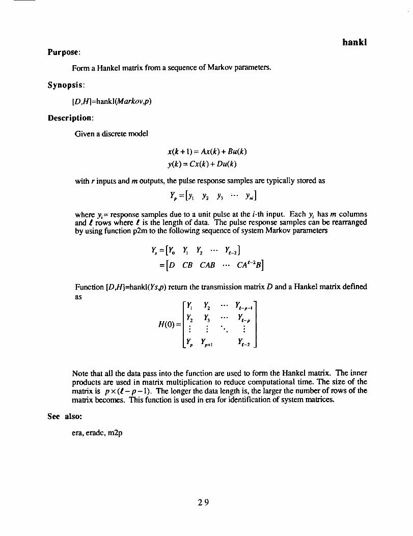
Purpose:

Form a Hankel matrix from a .sequence of Markov parameters.

Synopsis"

[D,H]=hankl(Markov,p)

Description"

Given a discrete model

x(k + 1) = Ax(k) + Bu(k)

y(k) = Cx(k) + Du(k)

with r inputs and m outputs, the pulse respon_ samples are typically stored as

Yp=[Y, Y2 Y3 "" Y,_]

where y_ = response samples due to a unit pulse at the i-th input. Each Yi has m columnsand l rows where ! is the length of data. The pulse response samples can be rearrangedby using function p2m to the following sequence of system Markov parameters

r,=[Vo v, ... v,_j=[D CB CAB ... CA t-2B]

Function [DJ1]=hankl(Ys,p) return the transmission matrix D and a Hankel matrix defined

as

[_ Y' ... h_,_,H(O)= r, ... Y,_,. ".. ."

Lv, r,÷, v,__

See

Note that all the data pass into the function are used to form the Hankel matrix. The inner

products are used in matrix multiplication to reduce computational time. The size of the

matrix is p x (l- p - 1). The longer the data length is, the larger the number of rows of thematrix becomes. This function is used in era for identification of system matrices.

also:

era, eradc, m2p

29

hankldc

Purpose:

Form a data correlation matrix from a sequence of Markov parameters.

Synopsis:

[D ,R ]=hankl( Markov _ )

Descri ption

Given a discrete model

x(k + 1)= Ax(k) + Bu(k)

y(k) = Cx(k) + Du(k)

with r inputs and m outputs, the pulse response samples are typically stored as

Yp=[Yl Y2 Y3 "'" Y,]

where y_= response samples due to a unit pulse at the i-th input. Each y_ has m columnsand t rows where l is the length of data. The pulse response samples can be rearrangedby using function p2m to the following sequence of system Markov parameters

r,=[ro=[D CB CAB ... CAt-2B]

From this sequence of Markov parameters, define two Hankel matrix as

i, r2 -.- ]

Y/-p-2

,qo=r2 r_ ... r__,,_,

: "'" YI-Yp+l 3

n __ [i"'" Y/p2

: °.

gp+l "'"

Yt,+l Yt,+2 "'" Yt-2

Function [D,R]=hankldc(Ys,p) returns the transmission matrix D and a data correlation

matrix R defined as

R = HHo r

See

Note that all the data pass into the function are used to form the data correlation matrix. The

size Of this matrix is (p + 1) x p which is independent of the length of the data. This

function is used in eradc for identification of system matrices.

also:

era, eradc, m2p

30

k abcd

Purpose:

Identify an Observer/Kalman filter gain matrix from test data for a discrete model to whitenthe stochastic residual.

Synopsis:

[G, Gmarl=k_abcd(A,B,C,D,u,y,p)

Description:

The function k_abcd solves for an observer/Kalman filter gain matrix of a system in theform

._(k + 1) = A_(k ) + Bu( k ) - Gly(k ) - _(k)]

_(k) = C._(k) + Du(k)

where ._(k) is the estimate of the state x(k) and ._(k) is the estimate ofy(k). The system has

m outputs, r-inputs, and time samples dt apart. The input/output time histories are stored ascolumn matrices. Initially an estimate of the desired observer Markov parameter number p

must be given for whitening the residuals. It is suggested that p is chosen such that theproduct p × m is greater than or equal to the order of the system. The identified matrix, G,and observer gain Markov parameters, Gmar (stored as a column matrix), are returned to themain program. See references for detailed information. To identify a stable observer whichwhitens the residual between the real output y(k) and the estimated output _(k), the system

matrices A, B, C, D, must be reasonably close to the true ones.

Example:

From the test data of a truss structure, use the function to compute a set of system matricesand an observer gain matrix. The order of the system is determined automatically by thefunction eradc. The residual is further whitened by using the function k_abcd to modify the

observer gain matrix. The function y_esti is used to compute the estimated outputs whichare then subtracted from the real output to obtain the residual. The following is output taken

from a typical run.

load sample|pt,il=size(u);|a,b,c,d,ml=okid(n,r,dt,u,y,'batch',20);

[time,y_e]=y_esti(a,b,c,d,m,u,y,dt,pt);[m 1,Cake] =k_abcd(a,b,c,d ,u,y ,20);[time,y_e 1]=y_esti(a,b,c,d,m 1,u ,y,dt,pt);clearabcd u

res=y-y__e;[yvt, vvt]-yycovar(n,2,pt,res, 1);clear resvvtwt =

2.1068e+02 -2.5208e+01-2.5208e+01 1.6014e+021.3304e+02 1.6889e+017.4350e+00 7.4626e+01

1.3304e+02 7.4350e+001.6889e+01 7.4626e+01

2.1061e+02 -2.5116e+01-2.5116e+01 1.6015e+02

31

res l =y-y__e l ;[yvt, vvt l ]=yycovar(res l ,2,1);clear res lvvtlwtl=

1.2454e+02 -4.8890e+01-4.8890¢+01 1.3218e+02-1.9179c+00 2.6610e-01-2.9991e+00 -1.4728e+01

- 1.9179e+002.6610e-011.2469e+02-4.8836e+01

-2.9991e+00-1.4728e+01-4.8836e+01

1.3220e+02

The mal_x

rr-:,<',_H res (l)

vvt = El l res_ (2)

Ltres (2).

resl(l) res2(1) rest(2)

res2(2)] 1

is the expected value of the auto- and cross-correlation of the residual obtained from theokid identified observer, whereas

rr,::,,,,>-!Alresl_(1) [,

vvtl = t_[ i resll (2 ) _resll (1)

[[resl2(2)J

resl2(l) resll(2)

resl2(2)]]

is obtained from the k_abcd identified observer gain using the okid identified system matrices.It is obvious that the residual resl is whiter than res.

Algorithm:

The algorithm used here is similar to that for the okid which identifies a set of systemmatrices, A, B, C, D, as well as an observer gain matrix, G. For given system matrices A,B, C, D, the deterministic component of the output can be subtracted out. The observergain is obtained by whitening the remaining residual. For details see references.

_ee also:

okid, okid_b, okid_fb, yycovar

References:

Ill Chen, C. W., Huang, J.'K., and Juang, J.-N., "Identification of Linear Stochastic Systems

Through Projection Filters," presented at the AJAA 33rd Structures, Structural Dynamics &Materials Conference, 1992, Paper No. AIAA-92-2520.

[2] Juang, J.-N., Chen, C. W., and Phan, M., "Estimation of Kalman Filter Gain from OutputResiduals" NASA Technical Memorandum TM-107603, Langley Research Center,Hampton, VA., March 1992.

32

m2pPurpose:

Rearrange a Markov parameters sequence in the form of pulse response time histories.

Synopsis:

Yp=m2p(Ys,r)

Description:

Given a discrete model

See

x(k + 1)= Ax(k) + Bu(k)

y(k) = Cx(k) + Du(k)

with r inputs and m outputs, the sequence of system Markov parameters is defined as

Y =[D CB CAB ... CAt-2B]

The pulse response samples are typically stored as

r,=[y, y2 y, "" Y,]

where yi= response samples due to a unit pulse at the i-th input. Each yi has m columns

and l rows where l is the length of data. The sequences Ys and Yp are equivalent in the

sense that both represent pulse response samples. The function converts Ys to Yp. Note

that Yp is the sequence used in the eradc and era functions.

If the combined system/observer Markov parameters (see function mar_com) are used, the

input matrix B becomes IB G] and the sequence Ys becomes

Y_=[D C[B G] CA[B G] "" CAt-2[B G]].

where the input number changes from r to r+m. The pulse response samples in Ypbecomes

Yp=[Yl Y2 Y3 "'" Y, Y,+I Y,+2 "'" Y,+m]

with m additional l x m matrices due to the observer gain matrix G which is treated as an

input matrix. The first r matrices represnt the system pulse response samples and the lastm matrices mean the observer gain pulse response samples.

also:

mar_com, okid, okid_b, okid_fb, p2m

33

mar_com, mar_sep

Purpose:

Recover the system Markov parameters from a set of observer Markov parameters.

Synopsis:

H=mar_com(ybar,r,n markov)H=mar_sep(yOb,y l b ,rg ,r,n_markov )

Description:

Given an observer of the form

"lfu(k )l

xtk l)=+ -Gl_y(k)f

y(k) = Cx(k) + Du(k)

with r inputs and m outputs, the sequence of observer Markov parameters previouslycomputed is passed to the function mar._com with

[o -c} cx{ -c} .. -c}]

or to the function mar_sep with

yOb=IC-B C'A-B C'A2-B ... C'A"-''*°'-'-B]and

ylb=[CG CA-G CA2G ... C'A"-'_°'-IG]

There is usually a small number, p, of nonzero observer parameters which is less thann markov. The observer matrices are related to the system matrices byA A + GC, B = B + GD, and D is the direct transmission term which is the same forsystem and observer. The function computes recursively n_markov parameters of the

original system and puts them in the form

H=[{O O} C{B -G} CA{B -G} "'" CAP{B -G}]

Algorithm:

The parameters are computed using the following recursive formula

k-!

CA'[B -G]=CA'B- ECAiGCA'-i-'[B -GI-CAkG[D O]i=0

for k=l,2,...n markov

34

Example:a=[0-0.16; 1 -11; b=[0 11';c=[0 11; d=0; G=[0.16 11';abar=a+G*c;

bbar=[b+G*d -G];

ybar=[d c*bbar e*abar*bbar];[H]=mar_com(ybar, l,2)

bg=lb -G1;Hs=[d 0 c*bg c*a*bgl

H

0 0 1.0000 -1.0000 -1.0000 0.8400

See

ns =

0

also:

okid, okid_b, okid_fb, okid_p

0 1.0000 -1.0000 -1.0000 0.8400

35

Purpose:mar oc

Compute a specified number of the system, observer, and controller Markov parametersfrom observer/controller Markov parameters ............

Synopsis:

[H]=mar_oc( Ybar ,r, rn,Ntotal)

Description:

From a sequence of observer/controller Markov parameters arranged in Ybar in thefollowing order

, and -F(A+GC)k-'[B+GD -G], k=l, 2,..., p

the function computes the following sequence of system, observer, and controller Markovparameters

[O]' I-C] [B -G], [gF]A[B -G] .... [CF]A_'ua-I[B -G]

that are arranged in the matrix H in this order. The scalar r denotes the number of inputs,

and m the number of outputs. Ntotal specifies the number of Markov parameters in H tobe returned to the user. For background information, the sequence of observer/controllerMarkov parameters are computed from closed-loop excitation data, and the function mar_oc

is then used to unscramble this sequence to obtain the system, observer, and controllerMarkov parameters.

Example:

load xsamp712ue(1:600)=I1;y(1:600)=ll;u(1:600)=11;[Ybar]=arxc(y,-u,ue,30,300);[H] =mar__oc (Ybar, 1,1,30)

n

Columns 1 through 7

-0.0689 0.1778 0.8012 0.0572 1.0144 0.1181 0.57740.0351 0.0422 -0.6740 -0.1063 -0.6234 -0.0419 -0.8527

Columns 8 through 14

0.0915 0.4184 -0.1442 0.2114 0.0086 0.0914 -0.1890-0.1076 -0.6742 -0.0692 -0.6106 0.0527 -0.3847 -0.0236

36

Columns15 through 21

-0.1854 -0.0041 -0.3831 -0.1030 -0.5743 -0.1404 -0.6633-0.1.319 0.1225 0.2654 0.0310 0.5776 0.1159 0.8443

Columns 22 through 28

-0.0318 -0.7223 -0.0736 -0.7292 0.0206 -0.7679 -0.10220.1240 0.9964 0.0591 1.0904 0.0730 1.1074 0.0075

Columns 29 through 35

-0.5967 0.0881 -0.4962 -0.0521 -0.2350 0.0872 -0.1258

1.0717 0.0602 0.8314 -0.0597 0.5758 0.0144 0.2073

Columns 36 through 42

0.0442 0.0852 0.0671 0.2845 0.1206 0.5419 0.0896-0.1010 -0.0944 -0.0799 -0.4433 -0.1145 -0.7440 -0.1510

Columns 43 through 49

0.7482 0.1712 0.8393 0.0375 0.9105 0.0575 0.8713- 1.0425 -0.1319 - 1.2376 -0.1653 - 1.2999 -0.0688 - 1.2899

Columns 50 through 56

0.0530 0.8104 0.0221 0.6379 0.0741 0.3764 -0.0248-0.0444 -1.1347 -0.0149 -0.8797 0.0075 -0.5058 -0.0365

Columns 57 through 61

0.1169 -0.0111 -0.1443 -0.1061 -0.3409-0.0961 0.0786 0.3044 0.0666 0.7439

Algorithm:

See

The system, observer, and controller Markov parameters are computed from the

observer/controller Markov parameters by a set of recursive equations. If more than pnumber of system, observer, and controller Markov parameters are required to be solved,the extra observer/controller Markov parameters are set to zero. For further details, seereferences.

also:

arxc, mar_yoc, ocid, ryucovar, separate

Reference:

Ill Juang, J. N. and Phan, M., "Identification of System, Observer, and Controller fromClosed-Loop Experimental Data," Presented at the AIAA Guidance, Navigation, andControl Conference, Hilton Head, South Carolina, Aug. 10-12, 1992.

37

mar_yoc

Purpose:

Compute system, observer, and controller Markov parameters directly from feedback

control input u/b, additive input excitation ue, and output resl:ionsey, '°

Synopsis:

[ocs ]=mar_ yoc (y, ufb ,ue ,p ,truncate ,Ntotal)

Description:

The function mar_yoc solves for the Markov parameters

I- C ] M_,i 1

[Do], [gF)B -G], [gF]A[B -G] .... L_FJA -[B -G]

from feedback control input ujb, additive input excitation ue, and output response y. Thedata is stored as column matrices. For example, for a system with m outputs, the closed-

loop output data matrix y contains m columns and as many rows as the number of data

points available. The data matrix uj'b contains the feedback control signal, ue contains the

additive excitation input signal. The number p denotes the number of observer/controller

Markov parameters to be solved. The number truncate specifies the number of data pointsto be deleted prior to application of the algorithm. This value is equal to the number of time

steps that is expected for the existing observer to converge. Ntotal is the total number of

Markov parameters to be solved for from p identified observer/controller Markovparameters. This is done by setting the extra observer/controller Markov parameters to bezero.

Fcq

[_FJAt-I[B -G]=O , k=p+l, p+2 ....

These Markov parameters are in the form ready to be used to obtain a state space realization ofthe system matrices, observer gain, and controller gain.

Example:

An example data file is contained in the file xsamp712.

load xsamp712[ocs]=mar_yoc(y,-u,ue,3,200,4)

OCS =

Columns 1 through 7

-0.0689 0.1778 0.8012 0.0572 1.0144 0.1181 0.5774

0.0351 0.0422 -0.6740 -0.1063 -0.6234 -0.0419 -0.8527

38

Columns8 through 14

0.0915 0.4184 -0.1442 0.2114 0.0086 0.0914 -0.1890-0.1076 -0.6742 -0.0692 -0.6106 0.0527 -0.3847 -0.0236

Columns 15 through 21

-0.1854 -0.0041 -0.3831 -0.1030 -0.5743 -0.1404 -0.6633-0.1319 0.1225 0.2654 0.0310 0.5776 0.1159 0.8443

Columns 22 through 28

-0.0318 -0.7223 -0.0736 -0.7292 0.0206 -0.7679 -0.10220.1240 0.9964 0.0591 1.0904 0.0730 1.1074 0.0075

Columns 29 through 35

-0.5967 0.0881 -0.4962 -0.0521 -0.2350 0.0872 -0.12581.0717 0.0602 0.8314 -0.0597 0.5758 0.0144 0.2073

Columns 36 through 42

0.0442 0.0852 0.0671 0.2845 0.1206 0.5419 0.0896-0.1010 -0.0944 -0.0799 -0.4433 -0.1145 -0.7440 -0.1510

Columns 43 through 49

0.7482 0.1712 018393 0.0375 0.9105 0.0575 0.8713- 1.0425 -0.1319 - 1.2376 -0.1653 - 1.2999 -0.0688 - 1.2899

Columns 50 through 56

0.0530 0.8104 0.0221 0.6379 0.0741 0.3764 -0.0248

-0.0444 -1.1347 -0.0149 -0.8797 0.0075 -0.5058 -0.0365

Columns 57 through 61

0.1169 -0.0111 -0.1443-0.0961 0.0786 0.3044

Algorithm:

See

-0.1061 -0.34090.0666 0.7439

The function first computes the observer/controller Markov parameters for the closed-loopsystem. Then, from the identified observer/controller Markov parameters, the individualsystem, observer, controller Markov parameters are computed and arranged in the specified

form which is ready to be used for realization. The function is a combination of thefunctions arxc and mar_oe.

also:

arxc, mar_oc, ocid, ryucovar, separate

39

Purpose: match

match system eigenvalues from identified forward and backward model and provide reducedforward and backward model in modal coordinates.

Synopsis:

[ lamdaf , bmf ,cmf ,msv_f ,lamdab,bmb,cmb ,msv_b l=match (af ,bf ,cf ,ab ,bb ,cb )

Description:

A typical forward state space model has the form

_,fu(k)1x(k + 1) : (A + GC)x(k) + [B + GD -Gl_y(k)_

y(k)-Cx(k)+ Du(k)

with m outputs, r inputs, and time samples dt apart. Here A, B, C, D are system matricesand G is referred to as the forward observer gain. The stable modes of the forward modelare inside the unit circle, whereas the unstable modes are outside the unit circle.

On the other hand, a typical backward state space model has the form

I-u(k)1x(k)=(A -! +GC)x(k + 1)+[-A-iB GD -G]/u(k +l) /

L y(k) J

y(k) = Cx(k) + Ou(k)

The stable _es of the backward model are outside the unit circle, whereas the unstablemodes are inside the unit circle. All matrices are the same as those described above for the

forward model, but here G is referred to as the backward observer gain matrix.

The matrices A, B, C, D, G, and t_ can be simultaneously identified by the functionokid_fb. For noise-free data, the A, B, C, D, identified either from the forward model or

from the backward model should have an identical input-output map, implying that theidentified system eigenvalues are identical. For noisy data, however, the system modes arecontaminated by the noises. In addition, there are many computational (spurious) modes inthe identified system matrices. As a result, the system matrices identified from both forwardand backward models are somewhat different because the system modes are contaminated

differently by noises. Note that the forward and backward models are identified byminimizing different residuals due to system uncertainties and measurement noises.Nevertheless, the system modes from both models should be reasonably close, whereas the

computational modes may be quite different. Therefore, matching is possible to distinguishthe system modes from the computational modes.

Given A, B, C identified for the forward model and A -t, -A-1B, C identified for thebackward model, function match return with a reduced forward model and backward model

in modal coordinates. The input parameters.af, bf, cfrepresent the forward model matricesA, B, C, whereas ab, bb, cb represent A-', -A-'B, Crespectively. The output vectors,lamdafand lamdab, contain the matched system eigenvalues for the forward and backward

models respectively. The matrices bmf, cmf, bmb,cmb are the corresponding input and

40

output matrices in modal coordinates, where the last character f means forward and bbackward. The output vectors msv_f and msv_b give the rosy (modal singular value, seefunction svpm) contribution to the pulse response samples for the forward and backwardmodal parameters, respectively. In addition to the eigenvalue matching, the rosycontribution is also examined. Those modes which has higher rosy contribution than thematched modes are also included in the reduced model. Therefore, both the reducedforward and backward modal models may not be the same in size. In general, the _ucedforward modal model is larger in size for stable modes than the reduced backward modalmodel. On the other hand, the reduced backward modal model may be larger in size forunstable modes than the reduced forward modal model. See references for detailedinformation. If the identified forward observer gain G and backward observer gain G are to

be counted in the computation of the rosy contribution, the input parameters bf should be

replaced by [bfgf] and bb by [bb gb], where gfmeans G and gb means G.

Example:

From two-input and three-output data of a three-mass-spring-dashpot system with twounstable modes and one stable mode, use okid and okid_b to identify a forward model and

backward model, and then match the identified eigenvalues. The input u and output y data

has 1 sec. sampling period, 250 data points and 10% noises.

[af, bf, cf,df, gf] =okid(3,2,1 ,u,y,'batch_lq',3);

[ab,bb,cb,db,gb] =okid_b(3,2,1 ,u,y,'batc h_lq',3);ab=inv(ab);bb=-ab*bb;[lamdaf, bmf,cmf, msv_f, lamdab,bmb,cmb,msv_b]=match(af,[bf gf],cf, ab,[bb gb],cb);n_b=length(lamdab);n_f=length(lamdaf);

eif=deg2hz(lamdaf, dt);disp([eif(:,1:2) msv_f]);

-1.4607e-01 2.7570e-01 2.5322e-01-1.4607e-01 2.7570e-01 2.5322e-01

-1.7733e-01 8.0889e-02 1.0000e+00-1.7733e-01 8.0889e-02 1.0000e+005.5570e-01 4.4269e-01 6.9444e-025.5570e-01 4.4269e-01 6.9444e-02

lamdab= 1.0 ./lamdab;bmb=-diag(lamdab)*bmb;

eib=deg2hz(lamdab,dt);disp([eib(:,1:2) msv_b]);

-1.8321e-01 2.7569e-01

-1.8321e-01 2.7569e-01-1.9672e-01 8.0897e-02-1.9672e-01 8.0897e-02

3.4786e-01 4.4260e-013.4786e-01 4.4260e-01

2.2238e-012.2238e-011.0000e+00

1.0000e+001.2439e-011.2439e-01

See also:

okid, okid_b, okid_fb, svpm

References:

[l] Juang, J.-N. and Phan, M., "Identification of Backward Observer Markov Parameters"Theory and Experiments," NASA Technical Memorandum TM-107632, Langley Research

Center, Hampton, VA., May 1992.

41

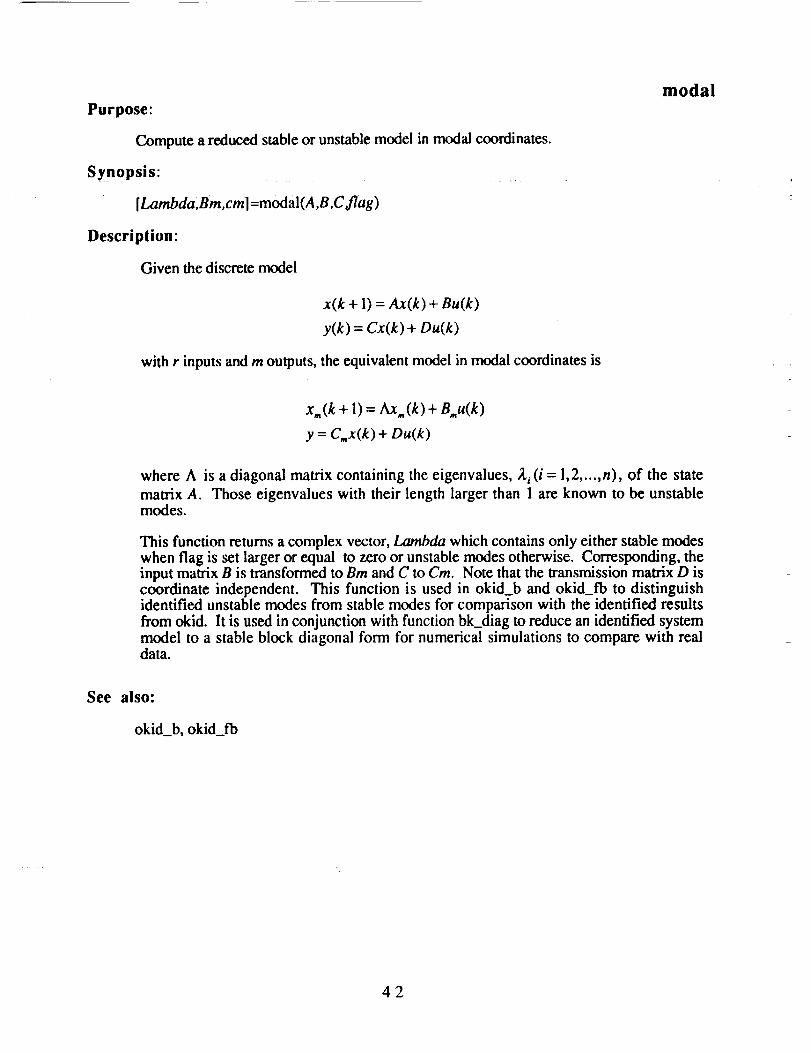
modal

Purpose:

Compute a reduced stable or unstable model in modal coordinates.

Synopsis:

[Lambda,Bm,cm| =m_a|(A,B,Cflag)

Description:

Given the discrete model

x(k + 1)= Ax(k) + Bu(k)

y(k) = Cx(k) + Du(k)

with r inputs and m outputs, the equivalent model in modal coordinates is

x.(k + 1) = Ax,.(k) + 8.u(k)

y = C,,,x(k) + Du(k)

where A is a diagonal matrix containing the eigenvalues, ,,q._(i = 1,2 ..... n), of the state

matrix A. Those eigenvalues with their length larger than 1 are known to be unstablemodes.

This function returns a complex vector,/_zanbda which contains only either stable modeswhen flag is set larger or equal to zero or unstable modes otherwise. Corresponding, theinput matrix B is transformed to Bm and C to Cm. Note that the transmission matrix D iscoordinate independent. This function is used in okid_b and okid_fb to distinguishidentified unstable modes from stable modes for comparison with the identified results

from okid. It is used in conjunction with function bk_diag to reduce an identified systemmodel to a stable block diagonal form for numerical simulations to compare with realdata.

See also:

okid_b, okid_fb

42

monera

Purpose:

Estimate variance of the ERA identified parameters.

Synopsis:

[e g ,e gm, vp ,vw,mh l=mone raO',m,r ,n,nm,dt,ni,nos ) ;

Description:

Monera uses the Monte Carlo approach to calculate the variance of the ERA identified

parameters contaminated by noise. The system pulse response samples y are stored as

.._

Yll (0) .-- Yml (0) "" Ylr(O) "" Ymr (0)

Y11(1) Yml (1) Ylr (1) Y,,w (1)

y11(2) ... yml(2) "-" ylr(2) .-. ym,(2)

yll(l--1) ... yml(l--l) "" yl,(l--1) "" y,,,,(l--ll

where yo(t) is the i-th output at discrete time t to a unit pulse at thej-th input. The system to

be identified has r inputs and m outputs. The identified model order, n, is chosen by theuser. Scalar nm specifies the row number of the Hankel matrix as described in era. Integers

nm x m should be greater than the model order n. Scalar dt specifies the data samplinginterval. Scalar ni specifies the number of the Monte Carlo runs used to estimate the varianceof the ERA identified parameters. Scalar nos specifies the standard deviation of the white,zero-mean and Gaussian measurement noise artificially added to the pulse response samples;nos should be much smaller than the root mean squared value of the pulse response samples

iny.

[eg,egm,vp,vw,mh]=monera(y,m,r,n,nm,dt, ni,nos) returns the eigenvalue vector eg andthe modal amplitude coherence vector mh of the ERA identified model from the pulseresponse samples y. The elements of vector egm are the mean values of the ni set of ERAidentified eigenvalues from the pulse response samples with added noise (nos). Vector vp(vw) is the variance of the ERA identified damping (frequency) corresponding to the

eigenvalue vector eg from ni set of Monte Carlo runs. The variable mh is the modalamplitude coherence.

43

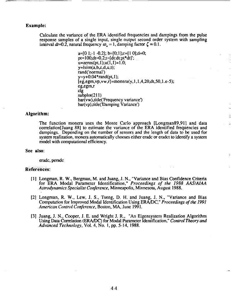
Example:

Calculate the variance of the ERA identified frequencies and dampings from the pulse

response samples of a single input, single output second order system with samplinginterval dt=0.2, natural frequency (o, = 1, damping factor _" = 0.1.

a=[0 1;-1 -0.21; b=[0;l];c=[l 0l;d--O;

pt= 100;dt=0.2;t=[dt:dt:pt dtl;u=zeros(pt, 1);u (1,1)= 1.0;y=lsim(a,b,c,d,u,t);rand('normar)y=y+0.04* rand(pt, 1);leg,egm,vp,vw,r]=monera(y,l,i,4,20,dt'50,1.e'5);eg,egm,rclgsubplot(211)bar(vw),title('Frequency variance')bar(vp),title('Damping Variance')

Algorithm:

The function monera uses the Monte Carlo approach [Longman89,91] and datacorrelation[Juang 881 to estimate the variance of the ERA identified frequencies anddampings. Depending on the number of sensors and the length of data to be used forsystem realization, monera automatically chooses either eradc or eradct to identify a systemmodel with computational efficiency.

See also:

eradc, peradc

References:

Ill Longman, R. W., Bergman, M. and Juang, J. N., "Variance and Bias Confidence Criteriafor ERA Modal Parameter Identification," Proceedings of the 1988 AAS/AIAAAstrodynamics Specialist Conference, Minneapolis, Minnesota, August 1988.

121 Longman, R. W., Lew, J. S., Tseng, D. H. and Juang, J. N., "Variance and BiasComputation for Improved Modal Identification Using ERA/DC," Proceedings of the 1991

American Control Conference, Boston, MA, June 199 I.

[31 Juang, J. N., Cooper, J. E. and Wright J. R., "An Eigensystem Realization AlgorithmUsing Data Con'elation (ERA/DC) for Modal Parameter Identification," Control Theory andAdvanced Technology, Vol. 4, No. 1, pp. 5-14, 1988.

44

ocid

Purpose:

Identify system, observer and controller gain matrices from closed-loop test data.

Synopsis:

[a,b,c,d,g fl=ocid(y,ufo,ue,p,dt,truncate,descripti°n)

Description:

The function ocid solves for the observer/controller Markov parameters of the following

system

_ru_(k) + u,(k)'x(k + 1) = (A + GC)x(k) + [B + GD - G]

y(k)L

I y(k) l I'C7• - i FiX(k) + Du(k)I_u, k J-L-j

with sampling time intervals dt apart. The data is stored as column matrices. For example,

for a system with m outputs, the closed-loop output data matrix y contains m columns and

as many rows as the number of data points available. The data matrix ufb contains thefeedback control signal, ue contains the additive excitation input signal. The number pdenotes the number of observer/controller Markov parameters to be solved for. The

number truncate specifies the number of data points to be deleted prior to application of thealgorithm. This value is equal to the number of time steps that is expected for the existing

observer to converge. The description is a short descriptive tag for the current data set and

indicates the computation procedure to be used to compute the observer and controller gain.

If the description is set to be 'lq', it means that a, b, c, d are realized first, and then g andf

are computed by least-squares (lq). Any other description indicates that a, b, c, d, g, andfare to be realized simultaneously. The function will first return a plot of singular values forthe user to select the desired model order. Once this is done, the function will ask whether

or not the user wants to see plots that show the actual responses and reconstructed

responses. Finally, a set of realized system matrices, observer gain, and controller gainwill be returned.

In general, if p observer/controller Markov parameters are to be solved for, then themaximum order of the system that can be recovered is pro, where m is the number of

outputs. The following rules apply with regard to the number of singular values computed.

If a flag value of zero is chosen, then the singular value plot will show (m+r)i singularvalues where i is the smallest integer such that (m+r)i is larger or equal to pm where r is

the number of inputs. If a flag value of one is chosen, then the singular value plot will

always show pm singular values. In either case, the user can always retain pm singularvalues to obtain a realized system that has the maximum order for a chosen value ofp.

The following information provides a better understanding of the OC1D problem. Considera linear discrete system of the form

45

which is operating

components

x(k + 1) = Ax(k) + Bu(k)

y(k) = Cx(k) + Du(k)

in closed-loop. The input to the system, u(k), consists of two

u(k) = UAk)

where u_(k) denotes the feedback signal provided by an existing linear state feedbackcontroller with gain F

uro(k ) = -Fj(k)

and u_(k) denotes an additive excitation input for closed-loop identification. The estimatedstate x(k) is provided by an existing observer of the form

._(k + 1) = A_(k) + Bu(k) - Ga[y(k) - _(k)]

_(k) = C_c(k)+ Du(k)

The output y(k) is the system closed-loop response due to an excitation ue(k). OCID firstsolves for the Markov parameters

o .....from which a realization of A, B, C, G, and F will be computed and returned to the user.Note that the matrices A, B, C, D are the system matrices and F is the existing feedbackcontroller gain as described above. The matrix G, however, is another observer gain

associated with the identifi _ system A, B, C, D. In general, this observer matrix gain G isnot the same as the existing ot_server gain G,_ of thecl0sed-loop system.'l_e m_x (7 is

an observer gain for the observer given below

./(k + 1)= A._(k)+ Bu(k)-G[y(k)- .9(k)]

.9(k) = C.i(k) + Du(k)

The function returns a, b, c, d, g, and f, which are a realization of A, B, C, D, G, and F.

Example:

Use test data from an aircraft flutter test. The items in italics is information prompted by thefunction ocid which has to be answered by the user. The rest is just general information

returned by the function ocid. The following is output taken from a typical run.

load xsamp712ue( 1:600)=[];y(1:600)=[1;u( 1:600)=[1;[m,nl=size(ue);time=dt* [0:m- 1]';

[a,b,c,d,g,f]=ocid(y,-u,ue,30,dt,300,'ocid');

ERADC is used now.

The Hankel matrix size for ERADC is 30 by 62.

46

MaximumHankelsingularvalue= 3.213077e+02Minimum Hankel singular value = 2.251935e-03

103

102

10-1

10-2

Hankel Matrix Singular Values

10-3 ......0 5 10 15 2O 25

Number

Desired Model Order (0=stop)=: 2Model Describes 98.9109 (%) of Test Data

Damping(%) Freq(HZ) Mode SV-3.2239e+00 9.1286e+00 1.0000e+00-3.2239e+00 9.1286e+00 1.00(K_+00

MAC9.9827e-019.9827e-01

30

Desired Model Order (0=stop)=: 4Model Describes 99.4891 (%) of Test Data

Damping(%) Freq(HZ) Mode SV2.2923e+01 1.1587e+01 5.7107e-022.2923e+01 1.1587e+01 5.7107e-02

-2.8767e+00 8.8912e+00 1.0000e+00-2.8767e+00 8.8912e+00 1.0000e+00

MAC

9.8650e-019.8650e-019.9987e-019.9987e-01

Desired Model Order (0=-stop)=: 8Model Describes 99.829 (%) of Test Data

Damping(%) Freq(HZ) Mode SV MAC1.8507e+01 1.9546e+01 1.2959e-02 9.4607e-011.8507e+01 1.9546e+01 1.2959e-02 9.4607e-01

2.9880e+00 8.7176e+01 2.2222e-02 9.8971e-012.9880e+00 8.7176e+01 2.2222e-02 9.8971e-011.6910e+01 1.1593e+01 9.2265e-02 9.9728e-011.6910e+01 1.1593e+01 9.2265e-02 9.9728e-01

-3.3582e+00 8.8459e+00 1.0000e+00 9.9995e-01-3.3582e+00 8.8459e+00 1.0000e+00 9.9995e-01

Desired Model Order (0=stop)=: 0

Compare closed-loop reconst, and actual resp. (l=yes,0=no) ?:= 1

47

O

<"O

60

40

20

0

-20

-40

-600

Number of sample points to reconstruct ?:= 400

Predicted open-loop and actual closed-loop responses

Output Number = 1

o'.5 i ' ' '1.5 2 2.5

Time (sec)

Actual vs. reconstructed closed-loop responses

_' 0.4

0.2

0

-0.2

-0.4_4

_" -0.6

<-0.8

0

Output Number = 1T r _ r

J

!

0.5 1 1.5 2

Time (sec)

/.,

2.5 3

48

Actual vs. reconstructed feedback control input histories

Input Number = 1

0.4

_ -O.2

| !0 0.5 l 2'.5 3Time (sec)

The solid lines represent the real data whereas the dashed lines mean the reconstructed data.

The predicted outputs are the reconstructed data from the identified system model only.The estimated outputs are the reconstructed data from the identified observer. It is obviousthat the reconstructed data match the real data very well.

Algorithm:

Identification of the observer/controller Markov parameters for the system shown before isobtained using a least-squares solution. The observer/controller Markov parameters areidentified first, from which the individual Markov parameters of the system, observer, andcontroller are computed, and used to obtain a realized state space model and the observerand controller gain matrices. For further details, see references.

See also:

arxc, mar_yoc, mar_oc, ryucovar, y closed, separate

Reference:

[]1 Juang, J. N. and Phan, M., "Identification of System, Observer, and Controller fromClosed-Loop Experimental Data," Presented at the AIAA Guidance, Navigation, andControl Conference, Hilton Head, South Carolina, Aug. 10-12, 1992.

49

Purpose:

okid,okid_b,okid_fb,okid_p

Identify a state space model and its corresponding observer from test data.

Synopsis:

[a,b,c,d,g]=okid(m,r,dt, u,y,description,p)[a,b,c,d,g] =okid_b(m,r, dt,y,description,p)[af ,bf ,cf ,df ,gf, ab, bb,cb ,db ,g b l=okid_fb(m,r,dt, u,y,des cription,p )

[a,b ,c,d,g ]=okid_p(m,r,dt,y,description,p )

Description:

The function [A,B,C,D,G]=okid(m,r,dt, u,y,description,p) identifies a state space model ofthe form

x(k + I)=(A +GC)x(k)+[B +GD

y(k)=Cx(k)+ Du(k)

with m outputs, r inputs, and time samples dt apart. Here A, B, C, D are system matricesand G is referred to as the forward observer gain. The input variable description is a short

descriptive tag for the current data set being analyzed and also serves as a flag which isdescribed latter. The input/output time histories are stored as column matrices. For sexperiments, the input matrix u must contain s x r columns and the output matrix y s x m.The number of rows in the input and output matrices equals the number of sample points.

Initially an estimate of the number of observer Markov parameters, p, must be specified.For a given p, the maximum system order that can be identified is the product p x m. Thefunction will prompt the user at various points for information. After computing theobserver Markov parameters, the option to compute the prediction error is given. Thecalculation of observer Markov parameters and the output prediction error is time consumingwhen analyzing long records, therefore, it should only be used when necessary. For thevery first run, the observer Markov parameters and related parameters including p are storedin the data file dokid_ffor function file okid, dokid b for okid_b, dokid_fb for okid_fb anddokid..p for okid_p. The user will be prompted if he has already stored these parameters inthe data file. If he did, computation of these parameters will be by-passed. A plot of the

Hankel matrix singular values is shown to aid selecting the correct system order. Thenumber of non-zero singular values equals the system order. The magnitude of the Hankelmatrix singular values, arranged in descending order, measures the state contribution. Fornoisy data, one has to make a judgement as to how many singular values to retain. Afterselecting a particular order, the percentage of the response realized by the model is computedusing the singular values. In addition, the corresponding frequencies and damping valuesare listed with the corresponding modal amplitude coherence factors. If the model isacceptable, the computation is completed. The identified matrices A,B,C,D, and G arereturned to the main program. See references for detailed information.

The user is recommended to run the batch job for the first time so that he does not have to

wait for the computation of observer Markov parameters which may take time for a longdata record. The user may then come back to run the same job again interactively and use

the existing data record for the observer Markov parameters.

50

The user is recommended to run the batch job for the first time so that he does not have towait for the computation of observer Markov parameters which may take time for a longdata record. The user may then come back to run the same job again interactively and use

the existing data record for the observer Markov parameters.

okid: It simultaneously identifies A, B, C, D and G directly from input/output data.User's interaction is required to determine the order of the system by looking at the

singular values plot.

description = "batch" ; It performs a batch job. The order of the system isdetermined internally in the era function file and thus user's interaction is not

required.

description = "lq" ; It computes the system matrices, A, B, C, and D, first and thenthe observer gain G using least-squares. Researchers who are interested inidentifying the system matrices only are recommended to use this function file.

okid_p: a modified version of okid, It uses pulse response samples, y, to simultaneouslyidentify A, B, C, D and G. No user inputs are required in this function file.

description = 'lq' ; It computes the system matrices, A, B, C, and D, f'trst and thenthe observer gain G using least-squares. Researchers who are interested inidentifying the system matrices only are recommended to use this function file.

The identified system has the following form

x(k + 1) = Ax(k) + Bu(k)

y(k) = Cx(k) + Du(k)

with its corresponding identified observer as

2(k + 1)= A/(k) + Bu(k)- Gly(k) - _(k)]

_(k ) = C_c(k) + Du(k )

where ./(k) is the estimate of the state x(k).

The function [A,B,C,D,G]=okid_b(m,r, dt, u,y,description_p) identifies a state space modelof the form

x(k) = (A -_ + GC)x(k + 1) +[-A-_B GD

y(k) = Cx(k) + Du(k)

[ u(k) ]

I_ y(k) .1

with m outputs, r inputs, and time samples dt apart. All the input and output parameters ofthis function are the same as those described above for the forward observer. Here A, B, C,D are system matrices and G is referred to as the backward observer gain matrix. Seereferences for detailed information.

51

okid_b: It simultaneously identifies A, B, C, D and t7 directly from input/output data.User's interaction is required to determine the order of the system by looking at the

singular values plot.

description = "batch' ; It performs a batch job. The order of the system isdetermined internally in the era function file and thus user's interaction is not

required.

description = "lq" ; It _omputes the system matrices, A, B, C, and D, first andthen the observer gain G using least-squares. Researchers who are interested in

identifying the system matrices only are recommended to use this function file.

The identified system is the same as above, whereas the observer becomes

£c(k ) = a-lYc(k + 1) + a-_ Bu(k )- Gly(k + 1) - _(k + 1)]

= c (k) + Du(k)where ._(k) is the estimate of the state x(k). Note that the backward approach identifies the

inverse of the system state matrix whereas the forward approach identifies the system statematrix directly. The advantage of the backward approach is that all the identified spuriousmodes tend to be stable and the strong system modes to be unstable. Therefore when theidentified state matrix is inverted, the strong system modes become stable but the

computational modes become unstable. Nevertheless, experiences suggest that theidentified results are somewhat underestimated particularly when noises are high. To donumerical simulations, functions modal and bk_diag may be used to reduce the identifiedmodel to a stable model in the real domain.

The function [Af, Bf ,Cf ,Df ,Gf ,Ab,Bb,Cb,Db,Gb ]=okid_fb(m,r,dt,u,y,description,p)identifies two state space models simultaneously using both the forward and backwardapproach. The small cases f and b behind the capital characters means forward andbackward respectively. In this function, comparison of stable system modes in terms of

frequencies and dampings from these two models is provided to the user for his judgementon how accurate the system modes are. The comparison is based on the error between theforward system eigenvalues and backward system eigenvalues, and their singular valuecontributions to the pulse response samples. The comparison provides the reduced outputforward model [Af, Bf, Cf, Df, Gj] and backward model [Ab,Bb, Cb,Db,Gb] where the statematrices Afand Ab are both in block-diagonal form (see function bk_diag). Note that thereduced modal observer may not be stable, since the modal reduction is not optimal in

general. In this case, the user is recommended to use function okid to identify a systemmodel and then reduced by other methods such as the optimal projection or balancedcoordinates. The function okid_fb is strongly recommeded for those users who do not careabout the observer identification. With the same order of observer markov parameters, it is

believed that the forward approach provides the identified results with better accuracy. Theforward model is in general larger in size than the backward model. The backwardapproach may miss some system modes particularly with light damping. However, it

provides information of strong system modes.

52

Example :

Use test data from a truss structure. The items in italics is information prompted by thefunction which has to be answered by the user. The rest is just general information returnedby the function. The following is output taken from a typical run.

load xsample[a,b,c,d,m] =okid_fb(n,r, dt,u,y,'okid_fb',20);

Total number of sample points = 2000Number of experiments in file = 1Number of inputs = 2Number of outputs = 2

Compute Observer Paramters For Data Set Number 1Time (min) to compute parameters 4.114

Have you run OKID_FB with the same data & P before (l=yes,0=-no) ?:= 0

0.02

o_-0.02

0

Compute Forward and Backward Error ( l=yes,O=no) ? =: 1

Compute Prediction Error For Data Set Number 1Forward Square Fitting Error Normalized

7.2631 e-02 -4.8648e-02-4.8648e-02 1.121 le-01

Backward Square Fitting Error Normalized1.5161e-01 -4.6554e-02

-4.6554e-02 1.4184e-01

Time (min) to Markov parameters 0.1517

i | ± 1 i i • | |

200 400 600 800 1000 1200 1400 1600 1800 2000

Time Steps

_0.02u.l

o

;_ -0.02 0

i

• 't ii: _ :, _I' _' " i : :_' _'' ,i

| I .... i I l I 1 I !

200 400 600 800 1000 1200 1400 1600 1800 2000

Time Steps

53

THE FOLLOWING COMPUTES A DISCRETE MODEL FROM A FORWARD OBSERVER.

Hankel Matrix Singular ValuesT103

102

101

10o

10-1

10-2

10-3

10-40

gggg

g

10 (5 2_0 2'5 30 3'5 40

Number

Desired Model Order (O=stop)= : 26Model Descdbes 99.9924 (%) of Test DataDamping(%) Freq(HZ) Mode SV MAC9.8448e+00 9.7606e+01 3.0499e-03 9.9677e-019.8448e+00 9.7606e+01 3.0499e-03 9.9677e-017.4294e+00 1.1862e+02 2.2901e-02 9.9957e-017.4294e+00 !.1862e+02 2.2901e-02 9.9957e-015.1193e+00 1.0573e+02 7.2535e-03 9.9891e-015.1193e+00 1.0573e+02 7.2535e-03 9.9891e-011.7537e+01 2.2577e+01 2.3866e-03 9.9869e-011.7537e+01 2.2577e+01 2.3866e-03 9.9869e-011.1365e+01 3.3578e+01 9.4557e-04 9.8801e-011.1365e+01 3.3578e+01 9.4557e-04 9.8801e-011.7740e+01 1.9096e+01 1.4288e-03 9.9687e-011.7740e+01 1.9096e+01 1.4288e-03 9.9687e-011.9292e+00 1.1410e+02 4.4511e-02 9.9999e-011.9292e+00 1.1410e+02 4A511e-02 9.9999e-013.4358e+00 6.1287e+01 1.6785e-03 9.9893e-013.4358e+00 6.1287e+01 1.6785e-03 9.9893e-011.4563e+00 4.6591e+01 1.222%-02 9.9996e-011.4563e+00 4.6591e+01 1.2229e-02 9.9996e-016.7864e-01 7.4241e+01 4.4470e-03 9.9929e-016.7864e-01 7.4241e+01 4.4470e-03 9.9929e-014.2429e-01 4.8646e+01 6.9666e-02 1.00(K_+004.2429e-01 4.8646e+01 6.9666e-02 1.0000e+003.1829e-01 7.2733e+00 4.8384e-01 1.000_+003.1829e-01 7.2733e+00 4.8384e-01 1.0000e+003.9005e-01 5.8479e+00 1.0000e+00 1.0000e+003.9005e-01 5.8479e+00 1.0000e+00 1.0000e+00

Desired Model Order (O=stop)= " 0

54

THE FOLLOWING COMPUTES A DISCRETE MODEL FROM A BACKWARD OBSERVER.

Hankel Matrix Singular Values1013

>

101o

107

104

101

10-2

10-5 .........0 5 10 15 20 25 30 35

Number

40

Desired Model Order (O=stop)= : 26

Model Describes 100 (%) of Test DataDamping(%) Freq(HZ) Mode SV MAC8.7805e+00 1.0444e+02 1.5233e-02 9.9862e-018.7805e+00 1.0444e+02 1.5233e-02 9.9862e-016.9248e+00 1.1904e+02 5.8056e-02 9.9986e-016.9248e+00 i.1904e+02 5.8056e-02 9.9986e-015.7392e+00 1.0529e+02 2.2203e-02 9.9896e-015.7392e+00 1.0529e+02 2.2203e-02 9.9896e-01!.9648e+00 1.1406e+02 8.8767e-02 1.0000e+001.9648e+00 1.1406e+02 8.8767e-02 1.0000e+007.0426e+00 3.1259e+01 2.6690e-03 9.8609e-017.0426e+00 3.1259e+01 2.6690e-03 9.8609e-012.6303e+00 6.1469e+01 2A191e-03 9.9780e-012.6303e+00 6.1469e+01 2.4191e-03 9.9780e-014.7085e+00 1.9505e+01 1.6134e-02 9.9995e-014.7085e+00 1.9505e+01 1.6134e-02 9.9995e-011.8700e+00 4.6542e+01 2.1705e-02 9.9976e-011.8700e+00 4.6542e+01 2.1705e-02 9.9976e-016.9673e-01 7.4489e+01 4.6185e-03 9.9365e-016.9673e-01 7.4489e+01 4.6185e-03 9.9365e-014.2593e-01 4.8600e+01 8.9072e-02 9.9999e-014.2593e-01 4.8600e+01 8.9072e-02 9.9999e-01

-8.8086e-01 5.8583e+00 1.0000e+00 1.0000e+00-8.8086e-01 5.8583e+00 1.0000e+00 1.0000e+00-9.3811e-01 7.3066e+00 3.9005e-01 9.9999e-01-9.381 le-01 7.3066e+00 3.9005e-01 9.9999e-01-1.9640e+01 1.4194e+01 3.1534e-02 1.0000e+00-1.9640e+01 1.4194e+01 3.1534e-02 1.0000e+00

Desired Model Order (O=stop)=." 0

55

COMPARISON OF FORWARD AND BACKWARD IDENTIFICATION

Forward Identification

Damping(%)1.7740e+011.7740e+013.4358e+003.4358e+001.7537e+01

1.7537e+011.4563e+001.4563e+006.7864e-016.7864e-019.8448e+009.8448e+005.1193e+005.1193e+004.2429e-01

Freq(hz)1.9096e+011.9096e+016.1287e+016.1287e+01

2.2577e+012.2577e+014.6591e+014.6591e+01

7.4241e+017.4241e+019.7606e+019.7606e+011.0573e+021.0573e+02

4.8646e+01

4.2429e-017.4294e+007.4294e+001.9292e+001.9292e+003.1829e-013.1829e-013.9005e-013.9005e-01

" 4.8646e+011.1862e+021.1862e+021.1410e+02

1.1410e+027.2733e+00

7.2733e+005.8479e+005.8479e+00

Mode SV1.8532e-031.8532e-033.2029e-033.2029e-033.2734e-033.2734e-031.3625e-021.%25e-02

1.7323e-02

1.7323e-022.8269e-022.8269e-025.7957e-025.7957e-02

7.3772e-027.3772e-022.0175e-012.0175e-013.2723e-013.2723e-01

4.4107e-014.4107e-011.0000e+00

1.00(K_+00

Backward Identification

Damping(%)1.9640e+01i.9640e+019.381 le-019.381 le-01

8.8086e-018.8086e-01

Freq(hz) Mode SV1.4194e+01 3.208 le-021.4194e+01 3.2081e-02

7.3066e+00 3.4642e-017.3066e+00 3.4642e-015.8583e+00 1.0000e+00

5.8583e+00 1.0000e+00

These are the modes selected from forward and backward modelsYou should al_ examine the list of modes from the forward modelto see if there are some other modes left out from the above table.

56

DATA RECONSTRUCTIONFROMTHE IDENTIFIEDFORWARDMODELCompare Recons. Output and True output (l=yes,O=no) ?:= 1

60

40

20

i °-20

-40

-600

:f20

_ 0

-20

-40

Number of Sample Points to Reconstruct ?:= I000

Comparison For Data Set Number No. 1The following figures show predicted and real outputs

Output Number = 1

a

i i , IJ

i!I

"i

! i i !

0.5 1 1.5 2 2.5

Time (sec)

Output Number = 2

h

i

3

r

t"

!i *J'¢ 'tI I:

i

3.5

..... j .... _ x

-_0 0.5 1 1.5 2 2.5

: i! • ,

4

0

r.

• i I

if-!t_

'!iI1

3 3.5

Time (sec)

4

4

57

60

40

20

m -20

-40

-6O0

40

30[

20

10

"_, -10U_

-20

-30

-400

The following figures show estimated and real outputs

Output Number = 1

A!1

!If ' !I

I

tii/!l

V

illY

0.5 1 1.5 2 2.5

Time (sec)

Output Number = 2r .......... _ ............ _r t ........... "1

li ,ii!_l

0.5 1.5 2 2.5

3 3.5 4

:1

V

3 315

I

!ii

li i:: ; : t

"I i.:vi!

,ii

4

Time (sec)

!

!

58

DATA RECONSTRUCTIONFROM THE IDENTIFIED BACKWARD MODELCompare Recons. Output and True output ( l=yes,O=no) ?:= 1

100

Number of Sample Points to Reconstruct ?:= 1000Comparison For Data Set No. 1The following figures show smoothed and real outputs

Output Number = 1

50

i °-50

, t ,'..i,,,,I t.

I:

? I'. t"

v "

:i II

!: II ""

f :l I_ i_ iI :4.: ! i :.

i: :

t

I I |

-1000 0.5 1 1.5

60

ol

f! ' :: _'l

t_ I

i .'....",;

,t

.: I:

I ,': I:

'_.I .

_,; iI

2

Time (sec)

2.5 3 3.5

Output Number = 2

4

20

i °-20

-40

ft:

Ii i:

,,:,/VI:Ili_!:.l_,_i,!'' _: V _I_ ' _ :1_ tt

I i." I. :lj

.I ii

.I

l,",,:/[ _,it:I,'_.\I:it it

t_iil!

0 ............ L ....... L ..............

0 0.5 1 1.5 2

Time (sec)

i I :

2.5t

3 3.5

ii!

4

59

The solid fines in the above figures represent the real data whereas the dashed lines mean thereconstructed data. The predicted outputs are the reconstructed data from the identifiedsystem model only. The estimated outputs are the reconstructed data from the identifiedobserver. It is obvious that the reconstructed data from the identified forward observer

match the real data much better than that from the identified model only. With the sameorder chosen which is 26 in this example, the forward results are somewhat better than thebackward results (see the reconstructed predicted outputs). In this example, only threestable modes (after the identified state matrix was inverted) are identified from the backward

approach.

Algorithm:

Identification of the pulse response (Markov parameters) for the observer system shown

before is obtained using singular value decomposition. The forward or backward observeris identified first, as opposed to the system itselT, Sui:h iliat ihe 0bserverhas all itspoiesplaced at the origin. From this, the system Markov parameters (pulse response) arerecovered and used in system realization. Theoretically, there are only a specific number ofindependent system Markov parameters for a finite set of observer Markov parameters.Therefore a minimum number of system Markov parameters may be used in the function eraor eradc to minimize the computational time in identifying the system. Nevertheless, itseems from experience that a little larger number than the minimum one for the systemMarkov parameters help a little bit for the identification of system with very low damping.The realization algorithm provides a state space model and permits the evaluation of differentsystem orders. Order selection is guided by the singular values of a Hankel matrix, but fortest data it is up to the user to decide. For details see references.

See Illso:

arx_b, arx_bat, arx_fb, era, eradc, k_abed, mar__com, match, pred_err, svmp, uy_stack,yucovar

References:

[ll Juang, J.-N., and Pappa, R. S.," An Eigensystem Realization Algorithm for Modal ParameterIdentification and Model Reduction," Journal of Guidance, Control, and Dynamics, Vol. 8,No. 5, Sept.-Oct. 1985, pp. 620-627.

[2] Juang, J.-N., Cooper, J. E., and Wright, J. R., "An Eigensystem Realization AlgorithmUsing Data Correlations (ERA/DC) for Modal Parameter Identification," Control-Theory andAdvanced Technology, Vol. 4, No. 1, 1988, pp. 5-14.

[31

[41

Juang, J.-N., Horta, L. G., and Longman, R. W., "Input/Output System Identification:Learning From Repeated Experiments," Mechanics and Control of Large Space Structuresedited by John L. Junkins, AIAA Monograph on Progress in Astronautics and Aeronautics,

Vol 29, 1990, pp. 87-99.

Chert, C. W., Huang, J.-K., Phan, M., and Juang, J.-N.,"Integrated System Identificationand Modal State Estimation for Control of Large Flexible Space Structures," Journal of

Guidance, Controland Dynamics, Vol. 15, No. 1, Jan.-Feb. 1992, pp. 88-95.

[5] Phan, M., Juang, J.-N., and Longman, R. W., "Identification of Linear Multivariable Systemsfrom a Single Set of Data by Identification of Observers with Assigned Real Eigenvalues,"Proceedings of the AIAA 32nd Structures, Structural Dynamics & Materials Conference,

60

Baltimore, MD., April 8-10, 1991, pp. 2325-2335, and to appear in the Journal of theAstronautical Sciences.

[6] Phan, M., Horta, L. G., Juang, J.-N., and Longman, R. W., "Linear System IdentificationVia an Asymptotically Stable Observer," Proceedings of the AIAA Guidance, Navigation andControl Conference, New Orleans, Louisiana, Aug. 1991, pp. 1180-1194, and NASATechnical Paper 3164, 1991, and to appear in the Journal of Optimization Theory and

Application.

[71 Juang, J.-N., Phan, M., Horta, L. G.,and Longman, L. G., "Identification of Observer andKalman Filter Markov Parameters: Theory and Experiments," Proceedings of the AIAA

Guidance, Navigation and Control Conference, New Orleans, Louisiana, Aug. 1991, pp.1195-1207.

[8] Horta, L. G., Phan, M., Juang, L-N., Longman, R. W., and Sulla, J., "Frequency Weighted

System Identification and Linear Quadratic Controller Design," Proceedings of the AIAAGuidance, Navigation and Control Conference, New Orleans, Louisiana, Aug. 1991, pp.1172-1179, and to appear in the Journal of Guidance, Control and Dynamics.

I91 Phan, M., Juang, L-N., and Longman, R. W., "On Markov Parameters in SystemIdentification," NASA Technical Memorandum TM-104156, Langley Research Center,

Hampton, VA., Oct. 1991.

[10] Juang, J.-N. and Phan, M., "Identification of Backward Observer Markov Parameters:Theory and Experiments," NASA Technical Memorandum TM-107632, Langley Research

Center, Hampton, VA., May 1992.

[11] Gawronski, W. and Juang, J. N., "Model Reduction for Flexible Structures," Advances inLarge Scale Systems Dynamics, Edited by C. T. Leondes, Academic Press, Inc., New York,

1990, pp. 143-222.

[12] Hollkamp, J.J. and Batill, S.M., "Automated Parameter Identification and Order Reductionfor Discrete Series Models," AIAA Journal, Vol. 29, No. 1, 1991.

[13] Hollkamp, J.J. and Batill, S.M., "Structural identification Using Order Overspecified Time-Series Models," Journal of Dynamic Systems, Measurement, and control, To appear.

61

Purpose:

Rearrange pulse response time histories in the form

Synopsis: .......

Yo=p2m(Yp, r)

Description" "

Given a discrete model

x(k + 1)= Ax(k) + Bu(k)

y(k) -- Cx(7_-+ DU(k)

p2m

of Markov pa_rameters sequ-e-nce.

with r inputs and m outputs, the pulse response samples are typically stored as

|

See

Yp=[Yl Y2 Y3 "'" Y,]

where y_= response samples due to a unit pulse at the i-th input. Each y_ has m columnsand I rows where l is the length of data. The sequence of system Markov parameters isdefined as

Yo=[D CB CAB ... CAt-2B]

The sequences Yo and Yp are equivalent in the sense that both represent pulse response

samples. The function converts Yp to Yo. Note that Yp is the sequence used in the eradcand era functions.

also:

m2p, okid, okid_b, okid_fb

62

peradcPurpose:

Calculate variance and bias of the ERA/DC identified parameters.

Synopsis:

[eg ,vp ,vw ,bp ,bw ,s g ,vs g ,bs g ]=peradc (y ,n,nm, nr ,dt) ;

Description:

The function peradc calculates the variance and bias of the single-input and single-outputeradc identified parameters from pulse response samples. The column vector y is the pulseresponse samples in which the ith element ofy is the unit pulse response at discrete time i.

Scalar n specifies the identified model order. Scalar nra(nr) specifies the number of rows(columns) of a Hankel matrix. In peradc, nr is required to be larger than or equal to rim.Scalar dt specifies the data sampling interval.

[eg,vp,vw,bp,bw,sg,vsg,bsgl=peradc(y,n,nm,nr,dt) returns the variance and quadraticbias of the eradc identified parameters. The elements of vector eg are the eigenvalues of theeradc identified model. Vector vp (vw) is the variance of the eradc identified dampings

(frequencies) corresponding to eigenvalue vector eg. Vector bp (bw) is the quadratic bias ofthe eradc identified dampings (frequencies) corresponding to eigenvalue vector eg. Vector

sg is the singular value vector of the correlation matrix in eradc. The elements in vector vsg(bsg) is the normalized variance (quadratic bias) of the singular values in sg.

Example:

Calculate the variance and bias of the eradc identified parameters from the noisy pulse

response samples of a single-input single-output second-order system with samplinginterval dt---0.2, natural frequency co = 1, and damping factor _"= 0.1.

a=[0 1;-1 -0.2]; b=[0;ll;c=[1 01;d--0;

pt=100;dt--0.2;t=[dt:dt:pt*dt]';u=zeros(pt, l);u(1,1)=l.0;

y=lsim(a,b,c,d,u,t);rand('normal')y=y+0.04*rand(pt, l);|eg,v p,vw,bp,bw,sg,v sg,bsg] =peradc(y,4,10,20,dt);

egclgsubplot(221)bar(vw),title('Frequency variance')bar(vp),title('Damping variance')bar(bw),title('Frequency bias')

bar(bp),title('Damping bias')

pauseclgsubplot(121)bar(vsg),title('Variance of singular values')bar(bsg),title('Quadratic bias of singular values')

63

Algorithm:

The function peradc uses the algorithm from [Longman89,91 ]. In peradc the perturbationtheory is applied to estimate the variance and quadratic bias of the ERA/DC identified

parameters.

See also:

monera, eradc

References:

[1] Longman, R. W., Bergman, M. and Juang, J. N., "Variance and Bias Confidence Criteriafor ERA Modal Parameter Identification," Proceedings of the 1988 AAS/AIAAAstrodynamics Specialist Conference, Minneapolis, Minnesota, August 1988.

[2] Longman, R. W., Lew, J. S., Tseng, D. H. and Juang, J. N., "Variance and BiasComputation for Improved Modal Identification Using ERA/DC," Proceedings of the 1991American Control Conference, Boston, MA, June 1991.

=

64

pred_efb, pred_erb, pred_errPurpose:

Compute the prediction error based on identified parameters.

Synopsis:

[errorf, yhaoq=pred_err(u,y, rf, p flag)[errorb,yhatb]=pred err(u,y,Yb,p flag)Ierrorf ,yhatf, errorb,yhatb l=pred_err( u,y, Yf ,Yb,p flag )

Description:

Given the input matrix u of dimension l x r, the output matrix y dimension I x m, and anestimate ofp forward observer Markov parameters stored in Yf, the forward prediction error

computed in matrix form is

where

%= g:- Y?:

yf = [y(0)y(1)---y(l - 1)1

YI= |o CB CAB ...

-u(0) u(D u(2)

v(0) v(1)vt=

[u(i)]v(i)=Ly(i)j;

v(O)

•.. u(t-1) ]/

-.- v(l-2) /

/•.. v(t- p- 1)j

i= 0,1, .... 1-1

See functions okid and arx_bat for the definition of matrices shown above. The number of

samples is 1 and the system has m outputs and r inputs. The computation is performedwithin a loop to reduce storage requirements at the expense of computation time. For caseswhere memory is not a problem flag=l yields faster computation time. The functionpred_err returns the prediction error in the vector errorfand the estimated measurement y inthe vector yharf.

Given an estimate ofp backward observer Markov parameters stored in Yb, the backward

smoothing error computed in matrix form is

e, =_y- r,v_where

65

u(0) u(l) u(2)

v(p) v(p+ 1) v(p + 2)K = _

kv(1) v(2) v(3)

y__= [y(O)yO)-..y(t-p -2)I

... u(l- p- 2)

... v(!- 2)

fu(i)]

v(i) = Ly(i)j;i=0,1 ..... l-1

• .. v(l-p-l)

...

See functions arx_b, arx_fb, okid_b and okid_fb for dcfinition of the matrices shown

above. The function pred__crb returns the backward smoothing error in the vector errorb

and the smoothed measurement y in the vector yha¢

Due to the strong similarity between the matrices VI and Vb, the forward and backwarderrors may be computed simultaneously. The function pred_efb returns the prediction error

in the vector errorf, the smoothing error in errorb, the estimated measurement y in yha(,

and the smoothed measurement y in yhatb.

Example:

See also:

m= 1;r=- 1;p=2;L=5;flag= 1;a=[0 -0.16; 1 -1]; b=i0 lr; c=[o 11; d=O; G=[0.16 1]';u=rand(L,r);

y=dlsim(a,b,c,d,u);abar=-a+G *c; bbar= Ib+G*d -G ];

Y=[d c*bbar c*abar*bbar];[error, yhat] =pred_err(u,y,Y,p,flag);

arx_bat

66

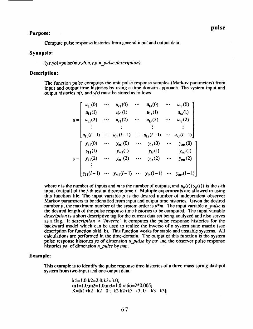
pulsePurpose:

Compute pulse response histories from general input and output data.

Synopsis:

[ys,yo]=pulse(m,r,dt, u,y,p,n_.pulse,description);

Description:

The function pulse computes the unit pulse response samples (Markov parameters) frominput and output time histories by using a time domain approach. The system input andoutput histories u(t) and y(t) must be stored as follows

U._--.

_

Ul_(O) --- u,_(o) ... u_,(o) -.. u,_(o)

Ull(1) Url (1) Uls(1) Urs(l )

utl(2) ..- Url(2) --- Uls(2) ... urs(2)

ujl(l-1 ) ... ud(l-1 ) ... uls(l-I ) ... Urs(l-1 )

Yl l (0) ... Yml (0) ... Yls (0) ... Yms (0)

Yll(1) Yml (1) Yls (1) Yms (1)

y1_(2) --- yml(2) --- yls(2) .-. y,,,s(2)

y_(l-l) ... yml(l-l) ... y_(l-1) -.- yms(l-1)

where r is the number of inputs and m is the number of outputs, and u_i(t)(y_i(t)) is the i-thinput (output) of the j-th test at discrete time t. Multiple experimentsare allowed in using

this function file. The input variable p is the desired number of independent observerMarkov parameters to be identified from input and output time histories. Given the desirednumber p, the maximum number of the system order is p*m. The input variable n__pulse isthe desired length of the pulse response time histories to be computed. The input variabledescription is a short descriptive tag for the current data set being analyzed and also servesas a flag. If description = 'inverse', it computes the pulse response histories for thebackward model which can be used to realize the inverse of a system state matrix (seedescription for function okid_b). This function works for stable and unstable systems. Allcalculations are performed in the time-domain. The output of this function is the system

pulse response histories ys of dimension npulse by mr and the observer pulse responsehistories yo. of dimension n_pulse by ram.

Example:

This example is to identify the pulse response time histories of a three-mass-spring-dashpotsystem from two-input and one-output data.

kl =1.0;k2=2.0;k3=3.0;ml=l.0;m2=l.0;m3=l.0;ratio=2*0.005;

K=[kl+k2 -k2 0 ; -k2 k2+k3 -k3; 0 -k3 k3];

67

Khalf=sqmn (K);Damp--ratio*Khalf;Ac=[zeros(3,3) eye(3,3);-K -Damp];Bc=[zeros(3,2);l 0; 0 I; 0 0];C=[zeros(1,5) 1];

dt=l.0;pt=200;p=10;[m,n]=size(C);[n,r]=size(Bc);D=-zeros(m,r);t=[dt:dt:pt*dt]';/A,B]=c2d(Ac,Bc,d0;rand('normal');

u=rand(pt,r);y=dlsim(A,B,C,D,u);[ys,yo]=pulse(m,r, dt,u,y,p,pt,'pulsc');%[ys,yo]=pulse(m,r,dt,u,y,p,pt,'inverse');% for backward only

Algorithm:

This is a time-domain approach. First, the forward or backward observer Markovparameters are identified (see arx_bat, arx_b), as opposed to the system itself, such that thecorresponding observer has all its poles placed at the origin. From these identified observerMarkov parameters, the system pulse response is recovered (see mar_com). For details seereferences.

See also:

arx_bat,arx_b,mar_com,m2p,okid,okid_b

References:

[1] Chen, C. W., Huang, J.-K., Phan, M., and Juang, J.-N.,"lntegrated System Identificationand Modal State Estimation for Control of Large Flexible Space Structures," Journal ofGuidance, Control and Dynamics, Vol. 15, No. 1, Jan.-Feb. 1992, pp. 88-95.

[2] Phan, M., Horta, L. G., Juang, J.-N., and Longman, R. W., "Linear System IdentificationVia an Asymptotically Stable Observer," Proceedings of the AIAA Guidance, Navigation andControl Conference, New Orleans, Louisiana, Aug. !99.1, pp. 1180-1194, and NASATechnical Paper 3164, 1991, and to appear in the Journal of Optimization Theory andApplication.

[3] Juang, J.-N., Phan, M., Horta, L. G.,and Longman, L. G., "Identification of Observer andKalman Filter Markov Parameters: Theory and Experiments," Proceedings of the AIAA

Guidance, Navigation and Control Conference, New Orleans, Louisiana, Aug. 1991, pp.1195-1207.

[4] Phan, M., Juang, J.-N., and Longman, R. W., "On Markov Parameters in SystemIdentification," NASA Technical Memorandum TM-104156, Langley Research Cente r,Hampton, VA., Oct. 1991.

[5] Juang, J.-N. and Phan, M., "Identification of Backward Observer Markov Parameters:Theory and Experiments," NASA Technical Memorandum TM-107632, Langley ResearchCenter, Hampton, "CA., May 1992.

!e

68

ryucovar

Pu r pose:

Compute the left correlation matrix associated with the feedback control input forobserver/controller identification.

Synopsis:

[ufoVt] = ryucovar(y,ufb,ue,p)

Description:

The data is stored as column matrices. For a system with m outputs, the closed-loop

output data matrix y contains m columns and as many rows as the number of data pointsavailable. The data matrix uJb cofitains the feedback control signal, ue contains the additive

excitation input signal in the same format as y. Let the given data be arranged as

Y=[y(O) y(l) y(2)..-y(N-1)]

U a,=[ua,(0 ) up,(1) u:,(2)-.-u_,(N-1)]

R=[u,(O) u,(1) u,(2).-, u,(N-1)]

The function ryucovar computes the following correlation matrix

uIbVt = U_,Vr

where the data matrix V is defined as

V

u(O) u(1) u(2) ... u(p) u(p+l) ... u(N-1)

z(0) z(1) -.- z(p-1) z(p) ... z(N- 2)

z(O) ... z(p- 2) z(p- 1) ..- z(N- 3)• . • . :

z(0) z(1) ... z(N- p- 1)

and z(k) is defined as

u_(k) + u,(k)z(k)=[ y(k) ]

As indicated, the number N specifies the number of data points to be used in the

computation. N can be less than the total number of data points available in ufl_, ue, and y.The matrix product returned by the function is used in the computation of theobserver/controller Markov parameters in the function ocid.

69

Example:

ufb-[1 -2 1 3 1 3 4 5 6]';

y=[O 3 2 1 3 1 446]';ue=[-I 0 2 -1 2 3 5 0 7]';

[ufbVt] = ryucovar(y,ufb, ue,2)ufbVt =

70 42 23 15 26

Algorithm:

To save memory space, the summations involved in the product U_Vrare performed using

inner matrix product multiplication.

See also:

ocid, arxc, mar_yoc, mar_oc, y_closed, separate

7O

Purpose:

Separate a given matrix sequence into two sequences with prescribed formats.

Synopsis:

[YI ,Y2] =separate(Y,q,m I ,m2)

Description:

Given a matrix Y in the following format

r=[Yt(l) Y_(2) Y2(1) Y2(2) ...... Y.(1) Y,(2)]

this function returns Y1 and Y2 which are

YI-[Y_(1) Y2(1)-.-Y,(l)]

Y2=[Y_(2) Y2(2)-.-Y,(2)]

Each Yi(1) has dimensions q ×ml, and each Y_(2) has dimensions q × m2.

Example:

Y=rand(2,9)

y=

Columns 1 through 7

0.9304 0.5269 0.6539 0.7012 0.7622 0.0475 0.32820.8462 0.0920 0.4160 0.9103 0.2625 0.7361 0.6326

Columns 8 through 9

0.7564 0.36530.9910 0.2470

[Y 1,Y2] =separate(Y,2,1,2)YI=

0.9304 0.7012 0.32820.8462 0.9103 0.6326

Y2=

0.5269 0.6539 0.7622 0.0475 0.7564 0.36530.0920 0.4160 0.2625 0.7361 0.9910 0.2470

See also:

arxc, mar_yoc, mar__oc, ocid, ryucovar, y_closed

separate

71

svpm

Purpose:

Compute modal observability matrix and singular values of the modal participation to the

pulse response samples.

Synopsis:

[svm, obsm]=svpm( lambda,bm,cm,n)

7

Descri ption:

Consider the discrete model in the modal coordinates

x.(k + 1)= Ax.(k) + B.u(tc)

y = C,_x(k)+ Du(k)

with r inputs and m outputs, where A is a diagonal matrix containing the eigenvalues,

_ (i = 1,2, .... n), of the system matrix. The modal observability matrix is computed by

obsm = q i

Lc, 7-'

Function [svm, obsm]=svpm(lambda,bm,cm,n) returns the complex modal

observability matrix and a normalized singular value vector svm (see algorithm) to

quantify the importance of each individual mode, for given system eigenvalues in the

vector lambda, the modal input matrix bin, modal output matrix cm and the desired

length n. Note that the maximum singular value is used to normalize the vector svm.

Example:

A three-mass-spring-dashpot system from two-input and three-output data is used.

kl =l.0;k2=2.0;k3=3.0;m 1= 1.0; m2= 1.0; m3= 1.0;ratio=2*0.005;

K=[kl+k2 -k2 0 ; -k2 k2+k3-k3; 0 -k3 k3];

Khalf=sqrtm(K);Damp=ratio*Khalf;Ac=lzeros(3,3) eye(3,3);-K -Damp];Bc=[zeros(3,2); 1 0; 0 1; 0 01;C=lzeros(3,3) eye(3,3)l;dt=l.0;pt=60;IA,B]=c2d(Ac,Bc,dt);[V,lambda]=eig(A);bm=V_B;crn=C*V;lambda---diag(lambda);[sv,obsvml = svpm(lambda,bm,cm,6);SV'

sv'= 0.2898 0.2898 1.0000 1.0000 0.1506 0.1506

72

Algorithm:

For a linear system, the map from input u to output y can be fully described by the

Markov parameter sequence

Y,,,=[D C.B,,, C,.AB,,, ... C,,,At-2B.]

This sequence is coordinate independent and unique. Let the input and output matrices

be partitioned as

I;1a.= ,c.=[c, c2 --- c.]

Lb.Jwhere n is the number of modal coordinates, bi (i=1,2 ..... n) a row vector of length r

and ci a column vector of length m. Each individual Markov parameter can then be

written as a combination of n components contributed from different modal coordinates.

C.AB,, = _ ciZ_b_i=1

Therefore, each coordinate has a sequence of Markov parameters described as follows

C l-2r, =[0 @, cAB, ... ,z, a,];i=1.2,....,,

The total Markov parameter sequence becomes

r.=_r.; r.o-[O o o ... o]i=0

From this representation, it is obvious that each modal coordinate contributes to the

pulse response sample by the individual modal sequence Y,,u, which can be quantified

by taking its maximum singular value, i.e.,

where IA._Iis assumed to be less than 1.

See also:

era, eradc, match

73

svraPurpose:

Identify a state space model from input and output data via a state vector realizationalgorithm.

Synopsis: _

lab c d eg sg]=svra(u y n nm nr dt k);

Description: .....

The functionsvra identifiesa state-spacemodel of a multi-inputand multi-outputlinear,tirne-invariantsystem from a setof richinputresponse data.The i-throw vectorof matrixu

(y)isthe system input (output)atdiscretetime i.Scalarn specifiesthe identifiedmodel

order.Scalarnm specifiesthe number of sample shiftinconstructingthe rows of a Hankelmatrix and itisrequiredtobe even, whereas nr specifiesthe column number of the Hankel

matrix.Integerstunx m(m isthe number of outputs)and nr are requiredto be not smaller

than the chosen model order n. Also, n + nm x r(r is the number of inputs)needs to be

smallerthaniv'.Scalaraftdenotes thedatasampling interval,and thedataused forrealization

startsfrom the k-thdiscretetime. [A,B,C,D,eg,sg]=svra(u,y,n,nm,nr,dt,kflag) returnsannth-orderlinear,time-invariantidentifieddiscretemodel:

x(k + 1) = Ax(k) + Bu(k)

y(k) = Cx(k)+ Du(k)

Vector eg contains modal parameters of the identified model including frequencies (Hz) in

the first column and damping ratios (%) in the second column. The third column of eg givesthe eigenvalues of the corresponding continuous time model. Note the identified discretemodel can be easily transformed to a continuous time model. Vector sg, whose elements aresingular values of the Hankel matrix, can be used as reference to choose the model order n.

Examples:

i) Use svra to identify a system model from a set of random input response data for a singleinput, single output second order system with sampling interval dt=0.3, natural frequencyto, = 1, and damping factor _"= 0.1.

ii) Transfer the identified discrete model to a continuous-time model and plot the originalsystem output and the output from the svra identified model.

|

74

a=[0 1;-1 -0.2]; b=10;l];c=[1 0];d=O;pt= 100;dt=0.4;t=[dt:dt:dt*pt]';rand('normar);u---rand(pt, 1);y=lsim(a,b,c,d,u,0;[a I ,b I ,c 1 ,d 1 ,sg,eg] =svra(u,y,2,20,40,dt, 10);yl=dlsim(al,bl,cl,dl,u);y2=[y yl];

clgplot(y2),title('Random input response')

pause• error=-y-yl;

clgplot(error),title('Error')pausesg

Algorithm:

The function svra uses the state vector realization algorithm from [Moonen89 Lew91]. Ituses output and input data to form the measurement malrix as

.._

Uk Uk+l ... Uk+nr_ 1

Yk Yk+l "'" Yk+nr-I

Uk+l Uk+2 • .. Uk+nr

Yk+l Yk+2 "'" Yk+nr. . • :

Uk+nm-I Uk+nm .'. Uk+nm+nr_ 2

Yk+nm-I Yk+nm "" Yk+nm+nr-2

where ui and Yi denote r-dimensional input vector and m-dimensional output vector at timei, respectively. In svra, the SVD of H is used for a state vector realization [Moonen89], i.e.

x_+Jk+m....,x_.__l.x_+j; j >> i. It then uses the following equation

:,.. x.,,)_, Yl+i "'" Yk÷_-l) "'" u_÷j-I

to identify a state-space model.

References:

[l] Moonen, M., Demoor, B., Vandenberghe, L. and Vandewalle, J., "On- and Off-LineIdentification of Linear State-Space Models," International Journal of Control, Vol. 49,1989, pp 219-232.

I2] Lew, J. S., Juang, J. N. and Longman, R. W., "Comparison of Several SystemIdentification Methods for Flexible Structures," Proceedings of the 32nd Structures,Structural Dynamics and Materials Conference, Baltimore, MD, April 1991, pp. 2304-2318.

75

Purpose:

Compute a stacked matrix with inputs and outputs.

Synopsis:

[vst ]=uy_stack (u,y,p )

Description:

Given a set of data with l .samples, r inputs, m outputs, and an assumed system order ofp'm, the function stacks a matrix using the inputs and outputs as follows

uy_stack

-u(0) u(l)

v(0)V=

u(2) ... u(t- 1)

v(1) -.- v(l- 2)

v(O) ... v(l- p-1)

i=0,1 ..... 1-1

The matrix dimension is [(r + m)p + r] x I

Example:

u=[0 1 2 3 4 5]';y=]6 7 8 9 10 1 lr;p=2;[vst]=uy_stack(u,y,p)vst =

0 1 2 3 4 50 0 1 2 3 40 6 7 8 9 100 0 0 1 2 3

0 0 6 7 8 9

See also:

arx_bat

D

76

y_closed

Purpose:

Reconstruct feedback control input and closed-loop response using oeid-identified system,

observer gain, and controller gain matrices.

Synopsis:

[ufb_rec,y_rec] =y_closed(A,B,C,D,G,F,y,ufb,ue)

Description:

Algorithm:

See

The function reconstructs the data histories ufb and y using the ocid-identified system

matrices A, B, C, D, identified observer gain G, and identified existing controller gain F.

The reconstructed t_,(k) , _(k) stored as column matrices in ufb_rec, y_rec, respectively,

are computed from the following equations.

._(k + 1)=(A + GC)_(k) +(B + GD)[ulb(k ) + u,(k)]-Gy(k)

Ctp,(k) = -F._(k )

Note that the above state equation equation is the same as the usual observer equation

expressed in terms of the prediction error y(k) - _(k)

_(k + 1)= A_(k) + B[u_(k)+u.(k)]-G[y(k)-_(k)]

= A_(k)+ B[up,(k)+u,(k)l-Gy(k)+G{C](k)+ D[ur.(k)+ u,(k)]}

=(A + GC)_c(k)+ (B + GD)[ur,(k) + u,(k )]-Gy(k )

The function is programmed using a Matlab function dlsim.

also:

ocid

77

Purpose:

Compute estimated outputs using an identified observer.

Synopsis:

[ t,yhat] =y_esti(a,b,c,d,G,u,y,dt, npts _ag)

Descri ption:

Any typical observer has the following form

y_esti

J(k + 1) = A_(k) + Bu(k) - Gly(k) - _(k)]

_(k) = CA(k) + Du(k)

See

where _(k) is the estimate of the state x(k) and ._(k) is the estimate of the output y(k). The

system matrices A, B, C, D, and the gain matrix G may be identified from input data u(k)

and output data y(k) using the function okid. The function

[t,yhatl=y._esti(A,B,C,D,G,u,y,dt, nptsJ'lag) returns a column vector, t, for the time period

corresponding to the desired number of sample points (npts), and an npts x m matrix, yhat,

for the estimated outputs. Theflag is set to 1 for plotting. The user will be prompted with

the desired number of sample points to be reconstructed. Plots will be given to show the

comparison between the real test outputs and the estimated outputs.

also:

okid, okid_b, okid_fb, y_pred

J

78

Purpose:

Compute predicted outputs using an identified system model.

Synopsis:

[t,yhat]=y_pred(a,b,c,d,u,y,dt, npts,flag)

Description:

The identified discrete system with the sampling time, dt, has the following form

y_pred

x(k + l) = Ax(k) + Bu(k)

y(k ) = Cx(k )+ Du(k )

where x(k) is the state vector. The system matrices A, B, C, D, and the gain matrix may be

identified from input data u(k) and output data y(k) using the function okid. The function

[t,yhat]=y_pred(A,B,C,D,u,y,dt, nptsJ'lag) returns a column vector, t, for the time period

corresponding to the desired number of sample points (npts), and an npts x m matrix, yhat,

for the reconstructed outputs. The outputs y(k) are used here for comparison with the

reconstructed outputs. Theflag is set to 1 for plotting. The user will be prompted with the

desired number of sample points to be reconstructed. Plots will be given to show the

comparison between the real test outputs and the reconstructed outputs.

See also:

okid, okid_b, okid_fb, y_.esti

79

yucovar, yucovfb, yucov_bPurpose:

Compute the left and right correlation matrices for least squares identification _roblem.

Synopsis:

lybarf, vbarf]=yucovar(u,y,p flag)[ybarb, vbarb ]=yucov_b(u,y,p )[ybarf, vbarf, ybarb, vbarb]=yucovfb(u,y,p)

=

Description: ..............

Given I sample points of a system with m outputs, r inputs, and an assumed system order

of p'm, the input matrix u is of dimension I x r whereas the output matrix y is 1 x m. The

flag is set to 1 for long histories. Let ybbe partitioned as

_yi=[y(O) y(1) y(2)---y(t-1)];

where each measurement y(i)(i=l,2 .... ) has the dimension m × 1. The least squaresproblem for the forward observer Markov parameters is posed as

Zlvf=Y 55"

The matrices. -yYV.r_ and VIV 7 have the same. structure as the cross and auto correlation asseen in the following

I-! 1-2l-p-1 ]

ZY(ii=o+ l)vr(i) ... ZY(ii=o+ plvr(i)j

1-1 1-2u(i)uT(i) _. u(i+l)vT(i)

i=0 i=0I-2 i-2_, v(i)uT(i+l) _. v(i)vT(i)

i=0 i=01-3 1-3_. v(i)uT(i+2) Y. v(i)vT(i+l)

i=0 i=0

l- -! " l-p-Iv(i)ur(i+p) _, v(i)vT(i+p-l)

i=0 i=0

1-3 I-_-IY u(i+2)vT(i) ... u(i+p)vT(oi=0 i=0

1-3 T i-_-1Y_v(i+l)v (i) ... v(i+p-1)vT(i)i=0 i=0

I-3 I-p-Iv(i)vT(i) ... _. v(i+p-2)vT(i)

i=0 i=0

l-p-I "- l-_-I_, v(i)vl(i+p-2)... _., v(i)vT(i)

i=0 i=0

where

i=O,1 .... ,l-1

The summations are performed using inner products to reduce computational time.

80

[ybarf, vbarJ]=yucovar(u,y,p flag) returns y fVf r and Vf V! r in ybarfand vbarfrespectively.

For the backward approach, let Yb be partitioned as

y_b=[Y(O) y(l) y(2)"'" y(l--p)];

where each measurementy(i)(i=l,2 .... ) has the dimension m x 1.

problem for the backward observer Markov parameters is posed as

The least squares

y,v -r v,v, TThe matrices Y_bVbr and VbVbr have the same structure as the cross and auto correlation as

seen in the following

Y_.bVbr =[tf_oY(i)ur(i) I-p l-p ]Ey(i)vr(i+ p) ... Ey(i)vr(i+ 1)i=0 i=0

VbVb7"=

l_flz,uri'u T_; (i) l- . l- l-_u(i)v'F (i+p) _Pu(i)vT (i+p-l) ... _u(i)vT (i+l)i=O i=0 i=0 i=O

l-p l-p l-p l-pY. v(i+p)uT(i) _, v(i+p)vT(i+p) _ v(i+p)vT(i+p-1) ... _, v(i+p)vT(i+l)

i=0 i=0 i=0 i=0

'_v(i+p-l)uT(i) l_v(i+p-l)vT(i+p) l-_v(i+p-l)vT(i+p-1) ... l-_v(i+p-1)vT(i+l)

i=0 i=0 i=0 i=0: ." : .,, ;

I- " l-p " I-p " I-p_v(i+l)uT(i) _, v(i+l)vT(i+p-1) _ v(i+l)vr(i+p-l) ... _, v(i+l)vr(i+l)

i=0 i=0 i=0 i=0

The summations are perfomw.d using inner products to reduce computational time.

[ybarb,vbarb l=yucov_b(u,y,p) returns.... YbV, r and VbVbr in ybarb and vbarb respectively.Note that there is noflag in mrs tunctioff.

The strong similarity among these matrices y Vf r, y Vbr, V V r and VbVbr suggests the• , --f. --b . f .

possibility of simultaneously compulang them m one single _unctmn.

[ybarf ,vbarf , ybarb,vbarb ]=yucovfb(u,y,p ) returns y fVf r, V;Vf r, YbVbr and VbVbr inybarf, vbarf, ybarb, and vbarb, respectively.

81

Example:

See also:

y=[56789]';p=2,flag=O;[ybar, ubar]=yucovar(u,y,p,flag)ybar _

80 50 200 26 146ubar --

30 20 70 II 56 ...........

20 14 44 8 38

70 44 174 23 128 _

11 8 23 5 20 _56 38 128 20 110 '

arx_bat, arx_b, arx_fb

. !

I

i

82

Purpose:

Compute the left and right output residual correlation matrices.

yycovar

Synopsis:

[yvt,vvt]=yycovar(y,p,iexp)

Description:

Given l sample points of a system with m output residuals (the stochastic part of the

system) and an assumed system order of p'm, the output residuals y is I x m. The flag isset to 1 for long histories. Let y be partitioned as

y=[y(O) y(1) y(2)-., y(/-1)];

where each y(i)(i= 1,2 .... ) has the dimension m x 1. The least squares problem for the

state estimator Markov parameters which whiten the residual is posed as

yV r = YVV rE

the matrices yV r and VV r have the same structure as the cross and auto correlation as seen

in the following

I-1 I-2

• .. y(i + p)yr (i)i=O

VV T .-

I-2 i-3 I-4 l--p-2

Y_y(i)yr(i) _y(i+ 1)yr(i) _.y(i + 2)yr(i) "'" XY(i + p-1)yr(i)i=O i=O i=O i=O

I-3 1-3 I-4 I'.p-2

_y(i)yr(i+l) _y(i)yr(i) _.y(i+l)yr(i) ... _y(i+p-2)yr(i)i=0 i=0 i=0 i=0I-4 I-4 i-4 l--p-2

_.y(i)yr(i+ 2) y_y(i)yr(i+ l) _ y(i)yr(i) "'" XY(i+ p-3)yr(i)i=O i=0 i=0 i=0

: : : ,,, :

" /- -2 "l- I- -2 . l- -2 "

-_2y(i)yr(i+ p) _y(i)y r(i+ p-1) _y(i)y r(i+ p-2) --- _y(i)y r(i)i=0 i=O i=0 i=0

where

_y=[y(l) y(2).., y(/-1)]

The summations are performed using inner products to reduce computational time.

[yvt, vvtl=yycovar(y,p,iexp) returns yV r and W r respectively in yvt and vvt.

83

Example: Some random numbers are created to verify the computation of this function.

rand('normar);y=rand(2,11);v=[y(:,1:10)];

yl=y(:,2:l 1);yl*v'ans =

-4.6867e-01 2.4383e+00- 1.0534e+00 -3.8444e+00

V*V'

ans =2.4726¢+00 -2.0860e+00

-2.0860e+00 1.3314e+01

y=y';lybar,ubarl=yycovar(y, 1,0)

ybar=-4.6867e-01 2.4383e+00-1.0534e+00 -3.8444e+00

ubar =2.4726e+00 -2.0860e+00

-2.0860e+00 1.3314e+01

See also:

kabed, arxbat

84

i

Form ApprovedREPORT DOCUMENTATION PAGE ONeNo.0 04-0I e

Pubhc reJ0ort=nq burden for th*_, collection of information _s est*mat_cl tO averaqP 1 hour i0e¢ response, mrtuding the time for reviewing instructions_ searching existing data sourc_c_,

gatherJncJ and ma,ntain=ng the data needed, and comtoleting and rewew*nq the collection of reformation ¢,end comments regard*ng this burden e_tlmate or any other aspect of this

colle<tion of information, mcludinq suqgest*on_ for roducmg this burden, to W.lshmqton =qe,_dquarters ¢.ervlces. DirectOrate tor Information Operations and Reports. 1215 Jefferson

Davis Highway. Suile 1204, Arlington, VA )220_-4 ]0. _, a.d to the Otfil e of M a.,*gement and Budget, P,}perwork Reduction Project (0)04-0188), Washington. DC 20503.

1. AGENCY'USE ONLY (Leave blank) 2. I_EPORTDATE | 3. REPORTTYPE AND DATES COVERED '

February 1992 I Technical Memorandum4. TITLEAND SUBTITLE 5. FUNDING NUMBERS ......

System�Observer�Controller Identification Toolbox

6.AUTHOR(S)

Jer-Nan Juang, Lucas Horta, and Minh Phan

7. PERFORMINGORGANIZATIONNAME(S) AND AOORESS(ES)

NASA Langley Research Center

Hampton, VA 23665-5225

9. SPOI_SORING/MONITORINGAGENCYNAME(S) AND ADDRESS(ES)

National Aeronautics and Space Administration

Washington, DC 20546-0001

WU 590-14-21-01

8. PERFORMINGORGANIZATIONREPORTNUMBER

10. SPONSORING/ MONITORINGAGENCY REPORTNUMBER

NASA TM-I07566

11. SUPPLEMENTARYNOTES

Jer-Nan Juang: Langley Research Center, Hampton, VA; Lucas Horta: Langley Research

Center, Hampton, VA; Minh Phan: Lockheed Engineering & Sciences Co., Hampton, VA.

12a. DISTRIBUTION/ AVAILABILITYSTATEMENT

Unclassified-Unlimited

Subject Category 39

1Zb. DISTRIBUTIONCOOt

13. ABSTRACT(Maximum200words)

System Identification is the process of constructing a mathematical model from input

and output data for a system under testing, and characterizing the system uncertain-

ties and measurement noises. The mathematical model structure can take various

forms depending upon the intended use. The SYSTEM/OBSERVER/CONTROLLER IDENTIFICATION

TOOLBOX (SOCIT) is a collection of functions, written in MATLAB language and

expressed in M-files, that implements a variety of modern system identification

techniques. For an open-loop system, the central features of the SOCIT are functions

for identification of a system model and its corresponding forward and backward

observers directly from input and output data. The system and its observers are

represented by a discrete model. The identified model and observers may be used for

controller design of linear systems as well as identification of modal parameters

such as dampings, frequencies, and mode shapes. For a closed-loop system, the

central features of the SOCIT include identification of an open loop model, an -

observer and its corresponding controller gain directly from input and output data.

14. SUBJECTTERMS

System Identification, Observer Identification, Controller

Identification, Modal Testing

17. SECURITYCLASSIFICATION 18. SECURITYCLASSIFICATIONOF REPORT OF THIS PAGE

Uriclass if led Unc lass if led

NSN 7540-O1-280-SSO0

19. SECURITYCLASSIFICATIONOF ABSTRACT

15. NUMBER OF PAGES86

16. PRICECOOE

A05

20. LIMITATION OFABSTRACT

Standard Form 298 tRey 2-89)Prescribed by ANSI _td Z39-18

_qR-1D2