ubiquitous & mobile computing

Copyrighted material; for CBU ICT Summer School 2009 student use only

Technische Universität Darmstadt

Telecooperation

Ubiquitous & Mobile ComputingConnectivity: Mobile Networks 1

Dr. Erwin Aitenbichler

Dr. Erwin AitenbichlerProf. Dr. M. Mühlhäuser

Telekooperation©

General Introduction – Connectivity

• Background: Elaborate Disciplines of– Computer Networks: connect computers around the world – Distributed Systems: software infrastructure atop Comp.Nets– what’s the distinction? well… not precisely defined, but:

• Dist. Systems establish a level of transparency atop Comp.Nets• … of locations, distribution, concurrency, performance…

• A very rough layering may look like this:

6. UC distributed application

2. Nodes i.e. computers (Resources, OS)

1. “Meshing”

distributed system: functionality, services

content/resource distribution

5. communication paradigm4. platform (middleware)

3. optional: overlay network

2


Telekooperation©

General Introduction – ConnectivityNotes about the “layers” shown on slide before:1. Meshing: how to interconnect adjacent computers

- today: mostly wired; since ~1990: shared switched media- UbiComp: wireless networks crucial

2. Nodes: apart from the mesh, computers are the resources added to system- today: mostly considered homogeneous (except: clients & servers for non-P2P)- today: resources mostly under control of computer owner- UbiComp: very heterogeneous nodes, resources partly ‘socialized’

3. Overlay Network- new: ‘socializes’ (some) resources from layer 2 ubiquitous distributed system- today: only used for special purposes (music exchange etc.)- UbiComp: increasing importance, towards general use

4. Platform: everything beyond 3 providing developers with ‘powerful, easy-to-use’ distr. sys.

- note: layers 3 & 4 use/contain the classical Internet layers TCP/IP etc.- today: 2 major purposes (same for UbiComp, but different (5), different services):

- providing basic services deemed useful for many applications/developers- implementing (5) via special protocols & bookkeeping instances

5. Communication abstraction: crucial for programmers!- today: mainly information pull, client/server paradigm- UbiComp: “push” dominates, but must embrace “pull”, too (see end of chapter)

6. Distributed applications themselves- today: rather ‘closed’ i.e. developed top-down by a team 3


Telekooperation©

Major Connectivity Trends in UC

6. UC distributed application

2. Nodes i.e. computers (Resources, OS)

1. “Meshing”

distributed system: functionality, services

content/resource distribution

5. communication paradigm4. platform (middleware)

3. optional: overlay network

new approach!lean! scalable!

services?

push!more elaborate! inte-gration w/pull, stream

scale!‚everyday‘ humans

& objects

wireless!!easy deployment;

integrating standards?

heterogeneity!federation,resou-rce ‚socialization‘?

Grid & P2P!content /compu-ting distribution?

4


Telekooperation©

Electromagnetic Spectrum

• VLF = Very Low Frequency• LF = Low Frequency• MF = Medium Frequency • HF = High Frequency • VHF = Very High Frequency• UHF = Ultra High Frequency• SHF = Super High Frequency• EHF = Extra High Frequency• UV = Ultraviolet Light

1 Mm300 Hz

10 km30 kHz

100 m3 MHz

1 m300 MHz

10 mm30 GHz

100 µm3 THz

1 µm300 THz

visible lightVLF LF MF HF VHF UHF SHF EHF infrared UV

optical transmissioncoax cabletwisted pair

f * λ = c (c: speed of light, 3* 108 m/s)

note: above figure showsorders-of-magnitude (log)

rules-of-thumb (remember!):1 MHz : 300 m100 MHz : 3 m10 GHz : 3 cm

5


Telekooperation©

Basics: 8* „Physics“ Laws & Observations

0. Beginner‘s Confusion don‘t mess up: carrier frequency ↔ bandwidth

1. Playground: electromagnetic spectrum• above FM (e.g. FM-Radio, ~ 108 Hz)• below visible light (~ 1015 Hz) in other words, mobComm uses• ~ microwaves 0.5 - 100 GHz or• ~ infrared > 100 THz

2. Rules-of-Thumb• signal energy ↔ data rate × reach (plus: observe rule 3.1 (-))

related to: electrosmog, advancements in EE, cost• the higher the frequency, the more behavior resembles that of light

– very low frequencies: „surface waves“– medium freq: e.g., reflection at ionosphere ...– very high freq.: „line-of-sight“ (cf. shadowing, distortion... below)

6


Telekooperation©


3. Carrier frequencies move up as R&D continues:

higher carrier frequencies mean ⇒1. (-) needs higher energy, more difficult (expensive) electronics2. (+) fewer competing „networks“ (a mess up to 2 GHz, difficult up to 10) 3. (+) larger bandwidths and/or # of channels ® higher data rates or more subscribers

examples:890 - 915 MHz (1990- today: GSM “uplinks”):5,1 – 5,8 GHz (2000 ff: Wlan 802.11a):59 - 62 GHz (20xx: future WLAN [“MBS”?], WiMax direct links in 50+ GHz)

(notes: 1. WLAN bandwidth still scattered: US 5,15-5,35 / 5,725-5,825,

EU 5,15-5,35 / 5,47-5,725; various [US/EU incompatible] energy leves 2. “MBS” has 3GHz of „space“, GSM uplink just 25 MHz)

7


Telekooperation©


4. Signal attenuation A („path loss“) is crucial• function of distance d, landscape, obstacles (buildings)• single most important difference to wired communications

(most substantial effect on protocol design etc.)!• A simple model for path loss

(A: mean received signal power, related to transmitted power):

– decreases w/ square of frequency

– decreases w/ power-of-α of distance (α = 2 in free space, up to 5 in urban environment)

A = (g: constant)

5. Signal path is crucial• highest attenuation: walls (steel?), signal „shadow“ (urban street?)• buildings reflection multipath distortion, interference !!• line-of-sight multipath: even different network designs!

Pr 1

Ps f2dα= g

8


Telekooperation©


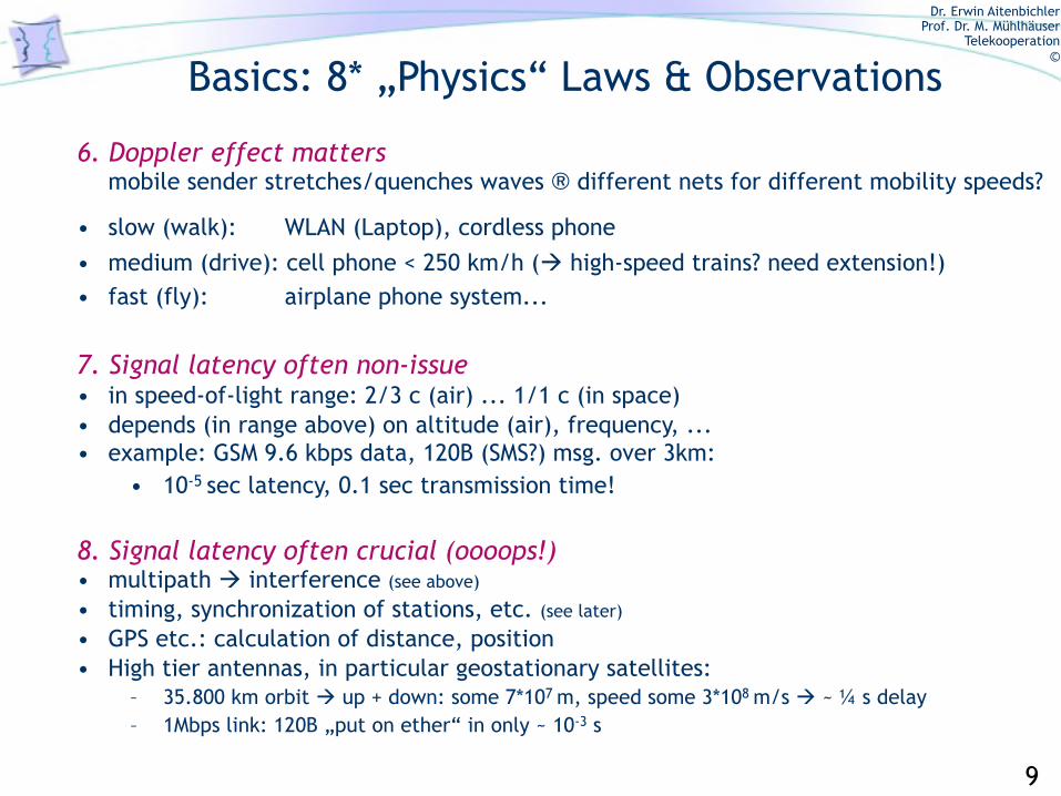
6. Doppler effect mattersmobile sender stretches/quenches waves ® different nets for different mobility speeds?

• slow (walk): WLAN (Laptop), cordless phone• medium (drive): cell phone < 250 km/h ( high-speed trains? need extension!)• fast (fly): airplane phone system...

7. Signal latency often non-issue• in speed-of-light range: 2/3 c (air) ... 1/1 c (in space)• depends (in range above) on altitude (air), frequency, ...• example: GSM 9.6 kbps data, 120B (SMS?) msg. over 3km:

• 10-5 sec latency, 0.1 sec transmission time!

8. Signal latency often crucial (oooops!)• multipath interference (see above)

• timing, synchronization of stations, etc. (see later)

• GPS etc.: calculation of distance, position• High tier antennas, in particular geostationary satellites:

– 35.800 km orbit up + down: some 7*107 m, speed some 3*108 m/s ~ ¼ s delay– 1Mbps link: 120B „put on ether“ in only ~ 10-3 s

9


Telekooperation©

Basics: „Physics“, Observations (6)

• recall attenuation: due to path loss• recall distortion: mainly due to multipath reflection• Further effects:

– shadowing (HiFreq: approaching 100%)– scattering (HiFreq: everyday objects [e.g., 30cm size])– diffraction: adds to attenuation, distortion

Summary of the four „obstacle“ effects

reflection scattering diffractionshadowing

10


Telekooperation©

Basics: SNR, Decibel

„design center“ of all networks (layer 1): Signal-2-Noise-Ratio SNR (or, S/R) i.e. power of ‚signal of interest‘ related to power of ‚what disturbs‘

Decibel: unit used to express relative differences in signal strengths. • given: two signals with powers P1, P2

• compute 10 * log10 (P1/P2)

• e.g.: P1 is 100 times P2:– P1/P2 = 100, log10 (100) = 2, ‚relation P1 : P2‘ is 20 dB

• ‚„relation‘ may be: SNR; power sent vs. received (attenuation); ...• e.g.: signal over 2 hops, no amplifier

– attenuation is 20:1, then 7:1 overall attenuation. is 140:1

– or: 13.01 dB + 8.45 dB = 21.46 dB (10*log1020 + 10*log107 = 10*log10140)

(note: power is f(amplitude2) 20*log10 (A1/A2) yields same result

11


Telekooperation©

Basics: ISI Peculiarities (1)

ISI (InterSymbol Interference) much different from wired networks

1. Hidden-Terminal Problem restricted listen-before-talk (LBT)• given goal: uncoordinated access of N senders to 1 medium • has risk of collision avoid by checking first if medium free• In example:

– S1 & S2 check: LBT o.k.– BUT: R experiences collision

(S2 may also be in „shadow“ of S1)

sender 1

reach (SNR>>0dB)

sender 2

receiver

receiver 1

sender 2

sender 1

receiver 2

2. Exposed-Terminal Problem LBT may be too pessimistic• In example:

– Both S1 and S2 could send– But S2 senses S1 during LBT

12


Telekooperation©

Basics: ISI Peculiarities (2)

ISI (InterSymbol Interference) much different from wired networks

3. Path Loss no listen-while-talk (LWT)• again goal: uncoordinated access of N senders to 1 medium • again: problem collisions detect, resolve• wire (Ethernet): LWT possible

– during Xmit: if signal-on-wire ≠ signal-sent: collision• wireless: LWT impossible (received signal much too low-energy)

4. Path Loss no full duplex traffic• wire (twisted pair): full duplex possible (2 peers use same wire)• wireless: needs two channels (= two carrier frequencies)

– mobile station MS base (transceiver) station BTS: „uplink“– base station mobile station: „downlink“ – (satellite jargon)

13


Telekooperation©

Basics: Cellular Networks

many categorizations of “cell sizes” exist! For our lecture: a) cell sizes (roughly) categorized according to radius, e.g.:

– pico: r = 50 m private (home, office) PicoNet– micro r = 500 m inner city (many users) wLAN, PLMN– macro r = 10 km ‚standard GSM‘; city, road PLMN– hyper r = 30 km rural area PLMN, HALO– overlay r = 200 km high tier antenna coverage HALO, LEO

Satellite

Macro-CellMicro-Cell

UrbanIn-Building

Pico-Cell

Global

Suburban

dik ©

b) categorizationaccording to‘outreach’:

BTS„coverage“ (reach): in reality, odd shape

r

cell

14


Telekooperation©

Basics: Cellular Networks

Roaming (option in cellular networks, some degree always supported):• MS may move freely between cells, even (!) switched-off • MS are “found”, identified upon switch-on (cf. incoming calls)Handover (option in cellular networks):• equals “roaming” during existing connection (active phone call)• connection „hand off“ to new cell• w/o interruption & noticeable effect to user(s)Home location register HLR:• admin. data in „home“ cell of subscriber• holds all permanent data of system-wide concern • may point at „current-VLR“, see belowVisitor location register VLR:• holds all admin. data relevant for the cell in which user „roams“

15


Telekooperation©

Multiple Access: Introduction (2)

• What is divided? ≥ four options (order ≈ tech. complexity):1. Space (SDMA):

• „bands“ are re-used at a certain distance (remote cell)• attenuation remote re-use won‘t interfere (much) with local cell

2. Frequency (FDMA):• different MS use different carrier frequencies• allocated frequency band divided into subbands• GSM900: 124*200kHz, GSM1800: 374*200kHz

3. Time (TDMA): • different MS use different time-slots• often: revolving frames, MS knows „its“ pos. (slot) in frame

4. Code (CDMA):• different MS use different „characteristic“ codes• receiver tunes to this code

16


Telekooperation©

Multiple Access: SDMA-1

• SDMA (SDM): frequency bands re-used in remote cells• different re-use patterns possible:

(repeated) clusters of cells– N = 3, 4, 7 (shown), 12, ... cells per cluster

– each band used only once per cluster

• design parameters:– reuse distance d=f(r,pattern)

– cell radius r (coverage)

• for different N (cluster sizes, patterns):– different d/r ratios different SNR

induced by remote cells of same band

– tradeoff: 1/N of all bands usable per cell

• realistic example (from Book by B. Walke):

1

23

45

6

7

1

23

45

6

7

1

23

45

6

7

1

23

45

6

7

1

23

45

6

7

1

23

45

6

7

1

23

45

6

7

d

d

17


Telekooperation©

Multiple Access: SDMA-2

1. channel assignment:• fixed: each cell has pre-assigned f‘s, for new calls & handover

• reservation: some f‘s reserved for handover• ‚borrowing‘ (from neighbors) ... totally dynamic

2. „Re-use related SNR“ (abstract from other noise)? E.g., N=7: – ...is called C/I ratio (C: carrier signal, I: interference sig.)

– remember path loss L = g⋅f–2⋅d-α (for fixed f: L= h⋅d-α )

– 6 neighbor BTSs w/ distance d (neglect others), max (BTSMS) = r

– see (figures, Pythagoras): d2 = (5⋅(½√3 r))2 + (r+½r)2 = 84/4 r2 = 21r2

– note: i) for carrier signal C: d=r; ii) let α=4; iii) 6 neighbors!

– C/I = (h⋅r-4) / (6⋅h⋅d-4) = d4/6r4 = 212r4/6r4 = 147/2 = 73,5 (18,66dB)

N=3: C/I=13.5=11.3dB (N=4: 16=12dB), but twice as many users possible

r

r

√ r2-¼r2 = ½√3 r

18


Telekooperation©

Multiple Access: FDMA

Example GSM900:

– carrier frequency of uplink/downlink Fu/Fd:

• Fu(n) = 890.2 MHz + (n-1) * 0.2 MHz, n=1 … 124

• Fd(n) = Fu(n) + 45 MHz

note: high-speed (wLAN, wATM etc.) increasing use of OFDM:overlapping bands, orthogonal frequencies (harmonic distances of

subcarriers, equals carrier distance) dyn. bandwidth assignment ...

frequency

time

channel 1

channel 2

channel 3

channel 4

channel 5

optional: gaps for better separationcarrier frequencies

Channels = subbands, distributed over available bandwidth

19


Telekooperation©

Multiple Access: TDMA

• Entire frequency dedicated to single sender-receiver pair, but only for a short period of time (time slot, slice)

• not applicable in analog transmission systems (old telephone net)• e.g., 9.6 kbps per channel > 80 kbps on ether for 8 channels• GSM: 8 slots (TDMA+FDMA!)• practical systems: TDMA always w/ FDMA

frequency

time

C1 C2 C3C0 C4 C5 C6 C7 C0 ........C7

Framesystem data („signaling“) channels = time slots

(1-in-many possible designs)

20


Telekooperation©

Multiple Access: CDMA

CDMA, also called „spread spectrum“ SS• versions: FH (FHSS), DS (DSSS) (chaotic crosstalk, but not ‚concurrent‘!)

• each sender uses “entire” bandwidth & time, „spreads“ code • Wideband (W-CDMA): plus FDMA, but huge subbands (~5MHz)

– Narrow (N-CDMA): smaller (~1MHz), but still >> FDMA+TDMA-subbands

• receiver knows coding rules of sender:– autocorrelations transforms signal back (to lo-bandwidth/hi-power)

– all other signals appear as noise ( # of senders limited, cf. TDM,FDM)

• no channel assignment simpler plus better spectrum utilization used in wireless LANs, increasingly in PLMN

• no synchronization needed (each code is self-synchronizing)• Problem: needs fine-grained transmission power control

– e.g., MSes must adjust such that all signals reach BTS w/ ~same power

– but: signal loss may change very fast (as MS moves)

– IS-95 (USA Qualcomm): 1kbps „adjustment channel“ per MS

21


Telekooperation©

Multiple Access: CDMA (FH)

Frequency-Hopping FH:

• Sender + receiver constantly change (hop-2-new) frequency– basis: pseudo-random sequence, initial value agreed

– origin: military networks (sequence unknown secret comm.)

• „Hope“: few collisions high probability of correction• Fast-FH: several / many hops per bit

– „a few“ collisions per bit don‘t harm

• Slow-FH: several bits per hop– GSM: optional (deterministic) slow-FH

• reason: distribute errors in „noisy“ bands over all channels • hope: corrected by forward-error-correction FEC

22


Telekooperation©

Direct Sequence (by far most commonly used):

• each bit mapped onto sequence of mini-bits (“chips”)• 10 chips / needs 10 times higher data rate (reality: up to ~1000)• Bit „1“ chip-sequence, Bit „0“ inverse sequence• receiver autocorrelates reconstructs original signal

– again: secrecy is by-product (IFF chip-seq. per station is random)SNR near 0 not even existence of communication detectable

– again: much more dynamic than FDM, TDM– plus: no (‚expensive‘) synchronous frequency-hopping needed!

Multiple Access: CDMA (DS)

“0” “1”

Note:in reality,Chip-seq.changesover time

23


Telekooperation©

Concurrent Access: ALOHA

• developed at U Hawaii (islands, hills!) since 1970: – wireless net connects terminals(/hubs) host system

– compares well to: MS BTS

– ‚grand father‘ of concurrent access schemes (wireless and Ethernet)

• channels: 407,350 MHz uplink, 413,475 downlink

– concurrent access (ALOHA) on uplink only

– downlink: packets + acknowledgements (ACK) for uplink packets

• MS send whenever packet ready• BTS sends corresponding ACK on downlink• if 2-or-more MS send with time overlap -> collision

-> BTS ignores „jam“ received -> no ACK

• MSes: timeout (no ACK received) -> send again -> collision repeated? no: since random „backoff“ (waiting time)

24


Telekooperation©

Concurrent Access: Pure ALOHA

• packets 1.1 (station A), 2.1 (B), 3.2 (C) transmitted ok• packets 1.2/3.1 collide, 1.3/2.2 too (partial as bad as total!)

receiptbasestation

total collision partial collisiontime

1.1 2.1 3.2

transmissions

station Apacket transmission time

1.1 1.2 1.3

station B 2.1 2.2

station C 3.1 3.2

25


Telekooperation©

Concurrent Access: Slotted ALOHA

• Fixed (maximum) packet size, equals time slots• common clock for slots (xmitted at downlink latency was rel. low)• start xmit w/ slot only (end ≤ slot end) all collisions are total• ‚surprise‘: mean throughput increased by factor of 2!

– why? xmission slightly later, but ‚just hit‘-overlaps avoided

1.1 1.2 1.3

2.1 2.2

3.1 3.2

station A

station B

station C

transmissions

1 2 3 4 5 6 7 8 9

1.1 2.1 3.21.3 2.2basestation

receipt

total collision

time

26


Telekooperation©

Concurrent Access: CSMA

Idea: stations ‚sense‘ channel before sending– CS = carrier sense („cs = on“ means: channel busy)

– CS also called LBT = listen-before-talk

• advantage: channel busy -> somebody sends -> don‘t disturb• total avoidance of collisions? NO

– MS1 ready2send, MS2 just started (signal has not arrived yet)

-> MS1: CS=off (no ‚busy‘ sensed) -> collision

• collision probability high at end of a transmission:– several MS want to send, sense channel during CS=on

• all MS realize CS=off immediate xmit

– CSMA variants therefore wrt. „when/how to start xmit“

27


Telekooperation©

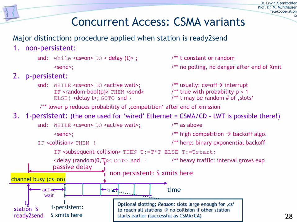
Concurrent Access: CSMA variantsMajor distinction: procedure applied when station is ready2send1. non-persistent:

snd: while <cs=on> DO < delay (t)> ; /** t constant or random

<send>; /** no polling, no danger after end of Xmit

2. p-persistent: snd: WHILE <cs=on> DO <active wait>; /** usually: cs=off interrupt

IF <random-bool(p)> THEN <send> /** true with probability p < 1 ELSE{ <delay t>; GOTO snd } /** t may be random # of ‚slots‘

/** lower p reduces probability of ‚competition‘ after end of xmission

3. 1-persistent: (the one used for ‘wired’ Ethernet = CSMA/CD – LWT is possible there!) snd: WHILE <cs=on> DO <active wait>; /** as above

<send>; /** high competition backoff algo. IF <collision> THEN { /** here: binary exponential backoff

IF <subsequent-collision> THEN T:=T*T ELSE T:=Tstart; <delay (random(0,T)>; GOTO snd } /** heavy traffic: interval grows exp

time

passive delaynon persistent: S xmits here

activewait

t0 1-persistent:S xmits here p - persistent:

channel busy (cs=on)

station Sready2send

slot

Optional slotting; Reason: slots large enough for ‚cs‘ to reach all stations no collision if other station starts earlier (successful as CSMA/CA) 28


Telekooperation©

Concurrent Access: CSMA/CA

• CA = collision avoidance; several minor variants as described here: ≈ slotted variant of p-persistent CSMA with p=0

• contention window CW = time interval considered collision intensive• after active wait; cs=off delay during IFS (interframe spacing)

– minimum IFS determined by wireless signal latency– 3 different IFSs (signal/priority/data: SIFS, PIFS, DIFS): priorities

• then:– draw random η ∈ [0,1)

– wait for slot that ‚contains‘ time η × CW (active wait: maybe cson)

η -> risk of collision ‚spread‘ over CW

– if still collision -> increase CW exponentially (up to maximum)

• fairness: if preceded by other station, # of slots waited count next time

time

xmit at slot startt0

channel busy

ready2sendIFS

CWdata

η x CW

slots 29


Telekooperation©Modulation (1)

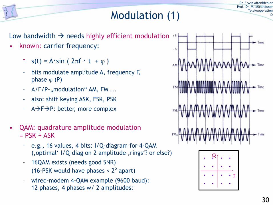
Low bandwidth needs highly efficient modulation• known: carrier frequency:

– s(t) = A.sin ( 2πf . t + ϕ )

– bits modulate amplitude A, frequency F,phase ϕ (P)

– A/F/P-„modulation“ AM, FM ...

– also: shift keying ASK, FSK, PSK

– AFP: better, more complex

• QAM: quadrature amplitude modulation= PSK + ASK– e.g., 16 values, 4 bits: I/Q-diagram for 4-QAM

(‚optimal‘ I/Q-diag on 2 amplitude ‚rings‘? or else?)

– 16QAM exists (needs good SNR)(16-PSK would have phases < 2o apart)

– wired-modem 4-QAM example (9600 baud):12 phases, 4 phases w/ 2 amplitudes:

I

Q

30


Telekooperation©Modulation (2)

• QPSK (Q=quadrature):– 4 phases: 0, 90, 180, 270 (a)– only phase changes, same amplitude– 2 bits per symbol (dibit)– Problem: 180° phase change -> zero crossing

-> decoding at receiver problematic,because temporarily no carrier

• π/4-QPSK– add 45° phase jump after each symbol,

independent of data– carrier signal always present

• OQPSK: Offset-QPSK– change of real part/imaginary part delayed by

half symbol time– max. phase change reduced to 90°

1100

01

10

11

00

01

10

or: b)a)

I

Q

31


Telekooperation©

Modulation (3)

• Advanced FSK: ambiguously called MSK, GMSK (GFSK unambiguous)• Example for M(F)SK below, gaussian filter would make it GFSK

data

even bits

odd bits

1 1 1 1 000

low frequency

highfrequency

MSKsignal

biteven 0 1 0 1odd 0 0 1 1

signal h l l hvalue - - + +

h: high frequencyl: low frequency+: original signal-: inverted signal

32

ubiquitous & mobile computing

Documents