ucla stat 110b linear regression analysis applied statistics for engineering and...
TRANSCRIPT
1
Stat 110B, UCLA, Ivo Dinov Slide 1
UCLA STAT 110BApplied Statistics for Engineering
and the Sciences
Instructor: Ivo Dinov, Asst. Prof. In Statistics and Neurology
Teaching Assistants: Brian Ng, UCLA Statistics
University of California, Los Angeles, Spring 2003http://www.stat.ucla.edu/~dinov/courses_students.html
Stat 110B, UCLA, Ivo DinovSlide 2
Linear Regression Analysis
Stat 110B, UCLA, Ivo DinovSlide 3
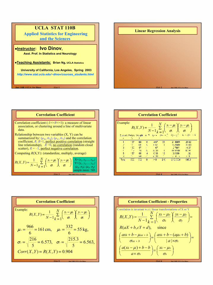
Correlation Coefficient
Correlation coefficient (-1<=R<=1): a measure of linear association, or clustering around a line of multivariate data.
Relationship between two variables (X, Y) can be summarized by: (µX, σX), (µY, σY) and the correlation coefficient, R. R=1, perfect positive correlation (straight line relationship), R =0, no correlation (random cloud scatter), R = –1, perfect negative correlation.
Computing R(X,Y): (standardize, multiply, average)
−
∑=
−
−=
y
yk
x
xk yN
k
xN
YXRσµ
σµ
111),(
X={x1, x2,…, xN,}Y={y1, y2,…, yN,}(µX, σX), (µY, σY)
sample mean / SD. Stat 110B, UCLA, Ivo DinovSlide 4
Correlation Coefficient
Example:
−
∑=
−
−=
y
yk
x
xk yN
k
xN
YXRσµ
σµ
111),(
Stat 110B, UCLA, Ivo DinovSlide 5
Correlation Coefficient
Example:
−
∑=
−
−=
y
yk
x
xk yN
k
xN
YXRσµ
σµ
111),(
904.0),(),(
,563.65
3.215 ,573.65
216
,kg 556
332 ,cm 1616
966
==
====
====
YXRYXCorr
YX
YX
σσ
µµ
Stat 110B, UCLA, Ivo DinovSlide 6
Correlation Coefficient - Properties
Correlation is invariant w.r.t. linear transformations of X or Y
−
=
×−+−
=
×
+−+=
−+
++
=
−
∑=
−
−=
+
+
x
xk
x
k
x
xk
bax
baxk
y
yk
x
xk
xa
bbxaa
babaxbax
dcYbaXR
yN
k
xN
YXR
σµ
σµ
σµ
σµ
σµ
σµ
)(||
)(
since ),,(11
1),(
2
Stat 110B, UCLA, Ivo DinovSlide 7
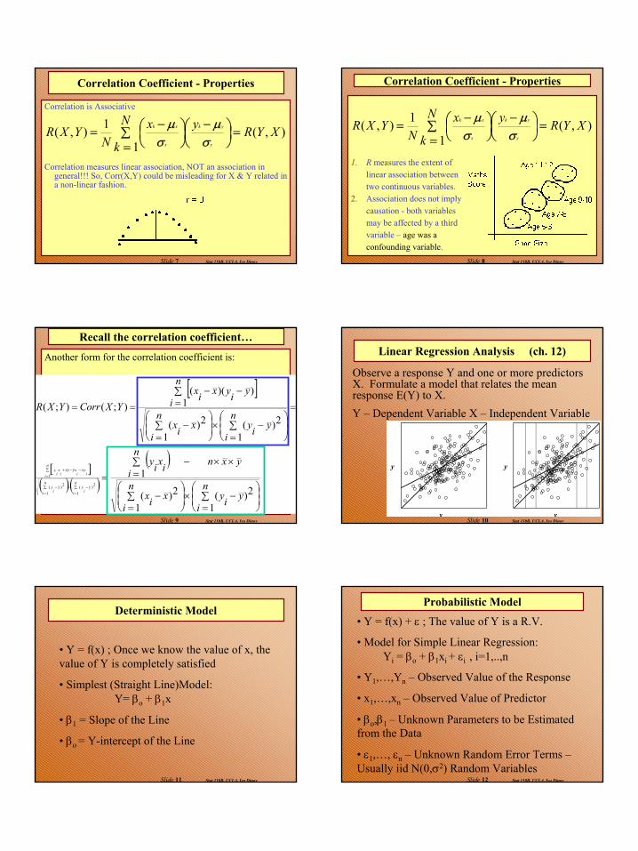
Correlation Coefficient - Properties
Correlation is Associative
Correlation measures linear association, NOT an association in general!!! So, Corr(X,Y) could be misleading for X & Y related in a non-linear fashion.
),(1
1),( XYRyN
k
xN
YXRy
yk
x
xk
=
−
∑=
−
=σµ
σµ
Stat 110B, UCLA, Ivo DinovSlide 8
Correlation Coefficient - Properties
1. R measures the extent oflinear association betweentwo continuous variables.
2. Association does not implycausation - both variablesmay be affected by a thirdvariable – age was a confounding variable.
),(1
1),( XYRyN
k
xN
YXRy
yk
x
xk
=
−
∑=
−
=σµ
σµ
Stat 110B, UCLA, Ivo DinovSlide 9
Recall the correlation coefficient…
Another form for the correlation coefficient is:
[ ]
[ ]( )( )
( )
∑=
−×
∑=
−
××−∑==
=
∑=
−×
∑=
−
∑=
−−
==
∑=
−×∑=
−
∑=
−−+
n
iyiy
n
ixix
yxnn
i ixiy
n
iyiy
n
ixix
n
iyiyxix
YXCorrYXR
n
iy
iy
n
ix
ix
n
i iyx
ixyyx
ix
iy
12)(
12)(
1
12)(
12)(
1))((
);();(
1
2)(1
2)(
1
Stat 110B, UCLA, Ivo DinovSlide 10
Linear Regression Analysis (ch. 12)
x x
y y
Observe a response Y and one or more predictors X. Formulate a model that relates the mean response E(Y) to X.Y – Dependent Variable X – Independent Variable
Stat 110B, UCLA, Ivo DinovSlide 11
Deterministic Model
• Y = f(x) ; Once we know the value of x, the value of Y is completely satisfied
• Simplest (Straight Line)Model: Y= βo + β1x
• β1 = Slope of the Line
• βo = Y-intercept of the Line
Stat 110B, UCLA, Ivo DinovSlide 12
Probabilistic Model
• Y = f(x) + ε ; The value of Y is a R.V.
• Model for Simple Linear Regression:Yi = βo + β1xi + εi , i=1,..,n
• Y1,…,Yn – Observed Value of the Response
• x1,…,xn – Observed Value of Predictor
• βo,β1 – Unknown Parameters to be Estimated from the Data
• ε1,…, εn – Unknown Random Error Terms –Usually iid N(0,σ2) Random Variables

3
Stat 110B, UCLA, Ivo DinovSlide 13
Interpretation of Model
For each value of x, the observed Y will fall above or below the line Y = βo + β1xaccording to the error term ε. For each fixed x
Y~N(βo + β1x , σ2)
Stat 110B, UCLA, Ivo DinovSlide 14
Questions
1. How do we estimate βo,β1, and σ2?
2. Does the proposed model fit the data well?
3. Are the assumptions satisfied?
Stat 110B, UCLA, Ivo DinovSlide 15
Plotting the Data
A scatter plot of the data is a useful first step for checking whether a linear relationship is plausible.
Stat 110B, UCLA, Ivo DinovSlide 16
Example (12.4)
A study to assess the capability of subsurface flow wetland systems to remove biochemical oxygen demand (BOD) and other various chemical constituents resulted in the following scatter plot of the data where x = BOD mass loading and y = BOD mass removal. Does the plot suggest a linear relationship?
x 3 8 10 11 13 16 27 30 35 37 38 44 103 142y 4 7 8 8 10 11 16 26 21 9 31 30 75 90
Stat 110B, UCLA, Ivo DinovSlide 17
Example (12.5)
An experiment conducted to investigate the stretchability of mozzarella cheese with temperature resulted in the following scatter plot where x = temperature and y = % elongation at failure. Does the scatter plot suggest a linear relationship?
Stat 110B, UCLA, Ivo DinovSlide 18
Estimating βo and β1
Consider an arbitrary line y = b0 + b1x drawn through a scatter plot. We want the line to be as close to the points in the scatter plot as possible. The vertical distance from (x,y) to the corresponding point on the line (x,b0 + b1x) is y-(b0 + b1x).
4
Stat 110B, UCLA, Ivo DinovSlide 19
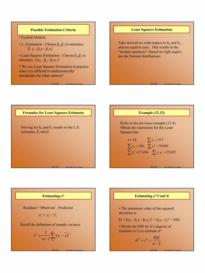
Possible Estimation Criteria
• Eyeball Method
• L1 Estimation - Choose βo,β1 to minimize Σyi - βox - β1xi
• Least Squares Estimation - Choose βo,β1 to minimize Σ(yi - βo - β1xi )2
* We use Least Squares Estimation in practice since it is difficult to mathematically manipulate the other options*
Stat 110B, UCLA, Ivo DinovSlide 20
Least Squares Estimation
Take derivatives with respect to b0 and b1, and set equal to zero. This results in the “normal equations” (based on right angles –not the Normal distribution)
Stat 110B, UCLA, Ivo DinovSlide 21
Formulas for Least Squares Estimates
Solving for b0 and b1 results in the L.S. estimates 10
ˆ and ˆ ββ
Stat 110B, UCLA, Ivo DinovSlide 22
Example (12.12)
Refer to the previous example (12.4). Obtain the expression for the Least Squares line
∑∑∑∑∑
==
==
==
825,25yx 454,17y
095,39x 346y
517x 14
ii2i
2ii
in
Stat 110B, UCLA, Ivo DinovSlide 23
Estimating σ2
Residual = Observed – Predicted
iii yye ˆ−=
Recall the definition of sample variance
∑=
−−
=n
ii xx
ns
1
22 )(1
1
Stat 110B, UCLA, Ivo DinovSlide 24
Estimating σ2 Cont’d
• The minimum value of the squared deviation is
D = Σ(yi - βox - β1xi )2 = Σ(yi - )2 = SSE
• Divide the SSE by it’s degrees of freedom (n-2) to estimate σ2
iy
2ˆ 22
−==
nSSEsσ
5
Stat 110B, UCLA, Ivo DinovSlide 25
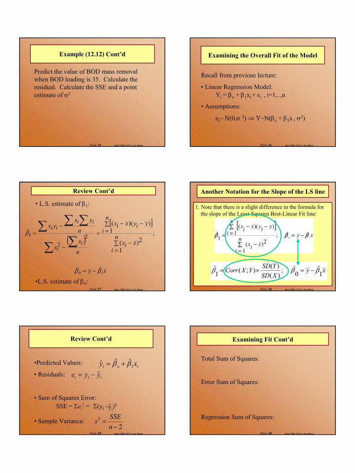
Example (12.12) Cont’d
Predict the value of BOD mass removal when BOD loading is 35. Calculate the residual. Calculate the SSE and a point estimate of σ2
Stat 110B, UCLA, Ivo DinovSlide 26
Examining the Overall Fit of the Model
Recall from previous lecture:
• Linear Regression Model:Yi = βo + β1xi + εi , i=1,..,n
• Assumptions:
εi~ N(0,σ 2) ⇒ Y~N(βo + β1x , σ2)
Stat 110B, UCLA, Ivo DinovSlide 27
Review Cont’d
• L.S. estimate of β1:
•L.S. estimate of β0:
( )[ ]
xy
n
ixix
n
iyiyxix
n
xx
n
yxyx
ii
iiii
10ˆˆ
;
12)(
1))((
ˆ2
2
1
ββ
β
−=
∑=
−
∑=
−−
=
−
−=
∑ ∑∑ ∑ ∑
Stat 110B, UCLA, Ivo DinovSlide 28
Another Notation for the Slope of the LS line
1. Note that there is a slight difference in the formula for the slope of the Least-Squares Best-Linear Fit line:
[ ]xyn
ixix
n
iyiyxix
10ˆˆ ;
12)(
1))((
1ˆ βββ −=
∑=
−
∑=
−−
=
xyXSDYSDYXCorr 1
ˆ0
ˆ ;)()();(1
ˆ βββ −=×=
Stat 110B, UCLA, Ivo DinovSlide 29
Review Cont’d
iy
•Predicted Values:
• Residuals:
• Sum of Squares Error:
• Sample Variance:
ioi xy 1ˆˆˆ ββ +=
iii yye ˆ−=
SSE = Σei2 = Σ(yi - )2
22
−=
nSSEs
Stat 110B, UCLA, Ivo DinovSlide 30
Examining Fit Cont’d
Total Sum of Squares:
Error Sum of Squares:
Regression Sum of Squares:
6
Stat 110B, UCLA, Ivo DinovSlide 31
Examining Fit Cont’d
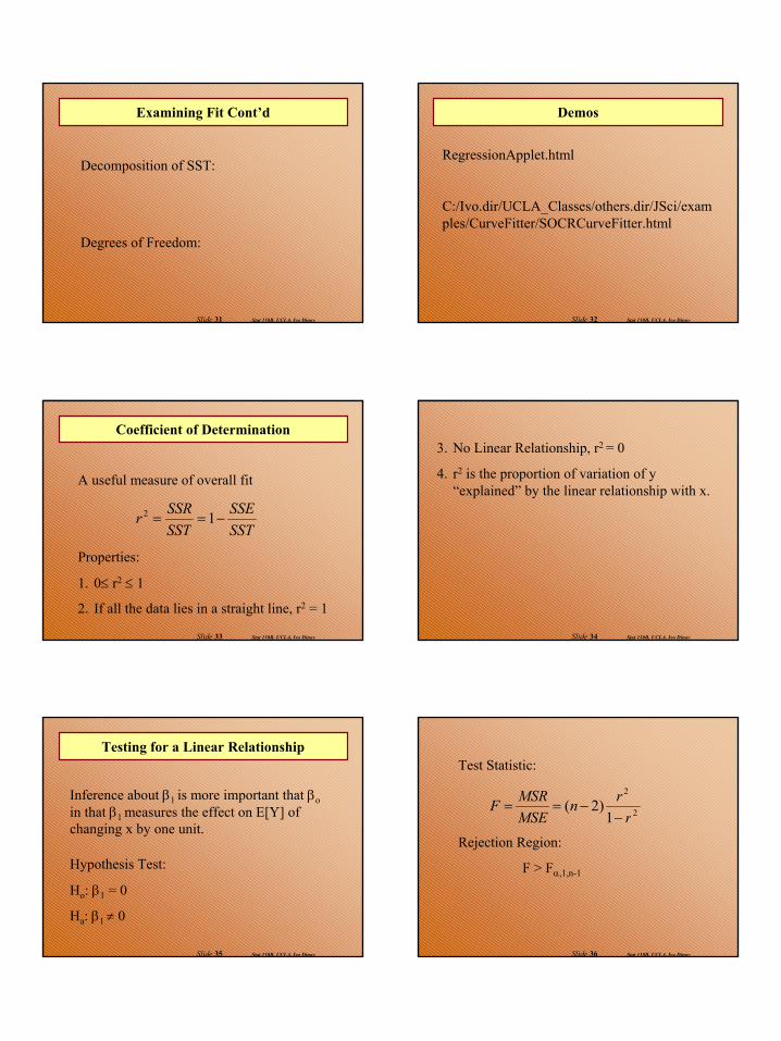
Decomposition of SST:
Degrees of Freedom:
Stat 110B, UCLA, Ivo DinovSlide 32
Demos
RegressionApplet.html
C:/Ivo.dir/UCLA_Classes/others.dir/JSci/examples/CurveFitter/SOCRCurveFitter.html
Stat 110B, UCLA, Ivo DinovSlide 33
Coefficient of Determination
A useful measure of overall fit
Properties:
1. 0≤ r2 ≤ 1
2. If all the data lies in a straight line, r2 = 1
SSTSSE
SSTSSRr −== 12
Stat 110B, UCLA, Ivo DinovSlide 34
3. No Linear Relationship, r2 = 0
4. r2 is the proportion of variation of y “explained” by the linear relationship with x.
Stat 110B, UCLA, Ivo DinovSlide 35
Testing for a Linear Relationship
Inference about β1 is more important that βoin that β1 measures the effect on E[Y] of changing x by one unit.
Hypothesis Test:
Ho: β1 = 0
Ha: β1 ≠ 0
Stat 110B, UCLA, Ivo DinovSlide 36
2
2
1)2(
rrn
MSEMSRF
−−==
Test Statistic:
Rejection Region:
F > Fα,1,n-1
7
Stat 110B, UCLA, Ivo DinovSlide 37
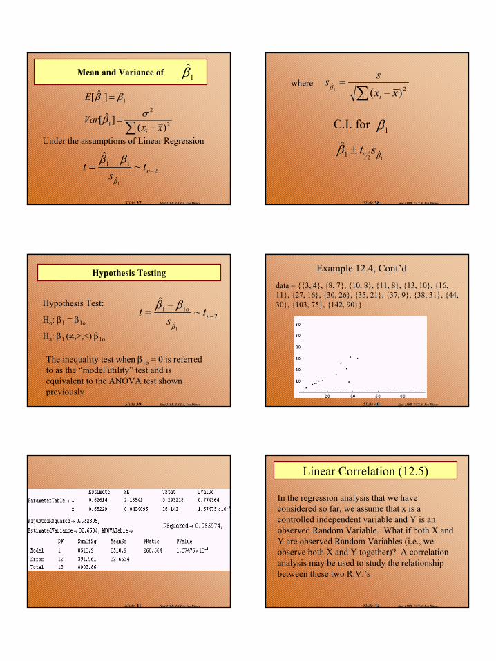
Mean and Variance of 1β
∑ −=
=
2
2
1
11
)(]ˆ[
]ˆ[
xxVar
E
i
σβ
ββ
Under the assumptions of Linear Regression
2ˆ
11 ~ˆ
1
−−
= ntst
β
ββ
Stat 110B, UCLA, Ivo DinovSlide 38
where∑ −
=2ˆ
)(1 xxssi
β
C.I. for 1β
12 ˆ1ˆ
βαβ st±
Stat 110B, UCLA, Ivo DinovSlide 39
Hypothesis Testing
Hypothesis Test:
Ho: β1 = β1o
Ha: β1 (≠,>,<) β1o
2ˆ
11 ~ˆ
1
−−
= no t
st
β
ββ
The inequality test when β1o = 0 is referred to as the “model utility” test and is equivalent to the ANOVA test shown previously
Stat 110B, UCLA, Ivo DinovSlide 40
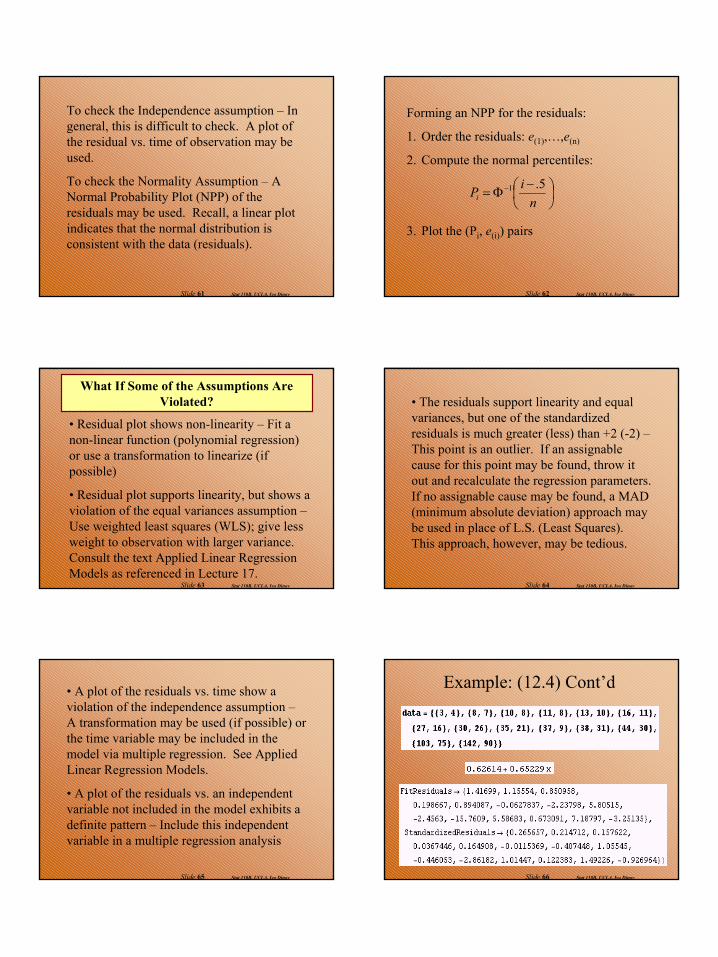
data = {{3, 4}, {8, 7}, {10, 8}, {11, 8}, {13, 10}, {16, 11}, {27, 16}, {30, 26}, {35, 21}, {37, 9}, {38, 31}, {44, 30}, {103, 75}, {142, 90}}
Example 12.4, Cont’d
Stat 110B, UCLA, Ivo DinovSlide 41 Stat 110B, UCLA, Ivo DinovSlide 42
In the regression analysis that we have considered so far, we assume that x is a controlled independent variable and Y is an observed Random Variable. What if both X and Y are observed Random Variables (i.e., we observe both X and Y together)? A correlation analysis may be used to study the relationship between these two R.V.’s
Linear Correlation (12.5)
8
Stat 110B, UCLA, Ivo DinovSlide 43
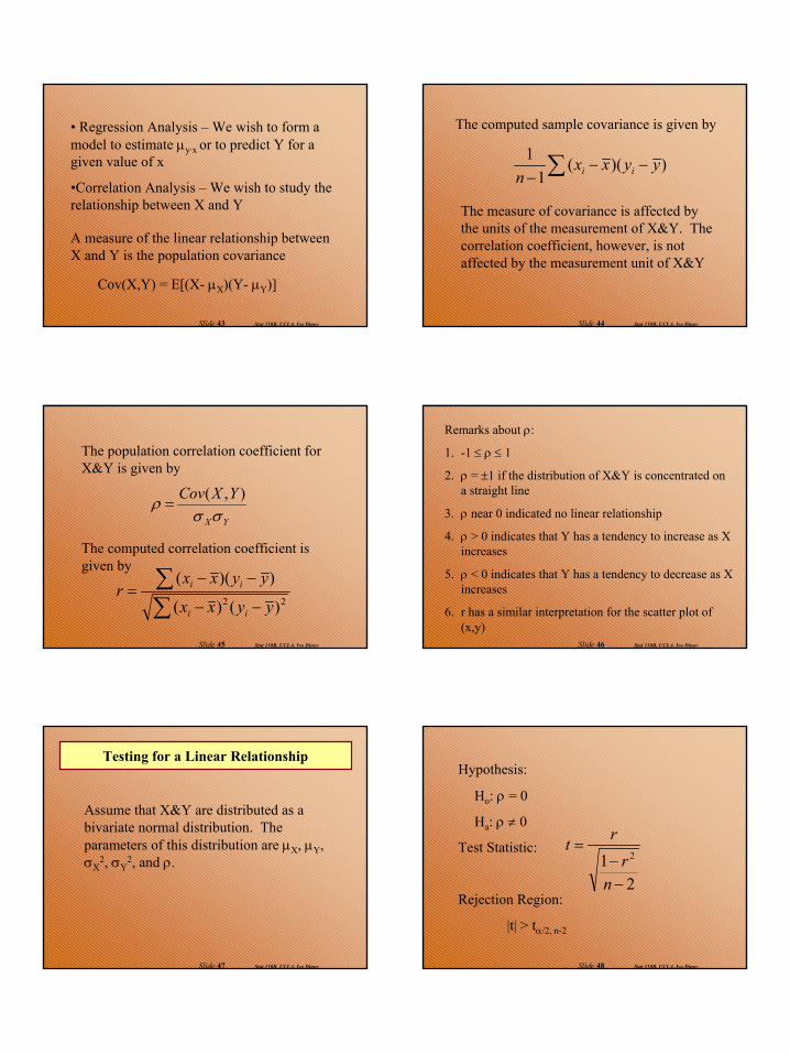
• Regression Analysis – We wish to form a model to estimate µy·x or to predict Y for a given value of x
•Correlation Analysis – We wish to study the relationship between X and Y
A measure of the linear relationship between X and Y is the population covariance
Cov(X,Y) = E[(X- µX)(Y- µY)]
Stat 110B, UCLA, Ivo DinovSlide 44
The computed sample covariance is given by
∑ −−−
))((1
1 yyxxn ii
The measure of covariance is affected by the units of the measurement of X&Y. The correlation coefficient, however, is not affected by the measurement unit of X&Y
Stat 110B, UCLA, Ivo DinovSlide 45
The population correlation coefficient for X&Y is given by
YX
YXCovσσ
ρ ),(=
The computed correlation coefficient is given by
∑∑
−−
−−=
22 )()(
))((
yyxx
yyxxr
ii
ii
Stat 110B, UCLA, Ivo DinovSlide 46
Remarks about ρ:
1. -1 ≤ ρ ≤ 1
2. ρ = ±1 if the distribution of X&Y is concentrated on a straight line
3. ρ near 0 indicated no linear relationship
4. ρ > 0 indicates that Y has a tendency to increase as X increases
5. ρ < 0 indicates that Y has a tendency to decrease as X increases
6. r has a similar interpretation for the scatter plot of (x,y)
Stat 110B, UCLA, Ivo DinovSlide 47
Testing for a Linear Relationship
Assume that X&Y are distributed as a bivariate normal distribution. The parameters of this distribution are µX, µY, σX
2, σY2, and ρ.
Stat 110B, UCLA, Ivo DinovSlide 48
Hypothesis:
Ho: ρ = 0
Ha: ρ ≠ 0
Test Statistic:
Rejection Region:
|t| > tα/2, n-2
21 2
−−
=
nr
rt
9
Stat 110B, UCLA, Ivo DinovSlide 49
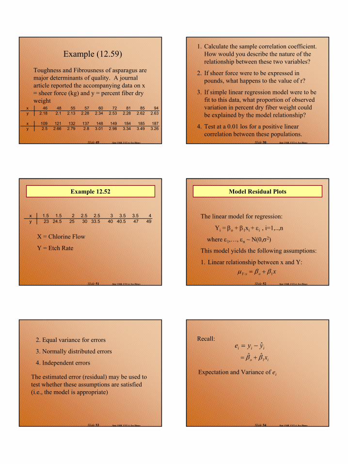
Example (12.59)
Toughness and Fibrousness of asparagus are major determinants of quality. A journal article reported the accompanying data on x = sheer force (kg) and y = percent fiber dry weight
x 46 48 55 57 60 72 81 85 94y 2.18 2.1 2.13 2.28 2.34 2.53 2.28 2.62 2.63
x 109 121 132 137 148 149 184 185 187y 2.5 2.66 2.79 2.8 3.01 2.98 3.34 3.49 3.26
Stat 110B, UCLA, Ivo DinovSlide 50
1. Calculate the sample correlation coefficient. How would you describe the nature of the relationship between these two variables?
2. If sheer force were to be expressed in pounds, what happens to the value of r?
3. If simple linear regression model were to be fit to this data, what proportion of observed variation in percent dry fiber weight could be explained by the model relationship?
4. Test at a 0.01 los for a positive linear correlation between these populations.
Stat 110B, UCLA, Ivo DinovSlide 51
Example 12.52
x 1.5 1.5 2 2.5 2.5 3 3.5 3.5 4y 23 24.5 25 30 33.5 40 40.5 47 49
X = Chlorine Flow
Y = Etch Rate
Stat 110B, UCLA, Ivo DinovSlide 52
Model Residual Plots
The linear model for regression:
Yi = βo + β1xi + εi , i=1,..,n
where ε1,…, εn ~ N(0,σ2)
This model yields the following assumptions:
1. Linear relationship between x and Y: xoxY 1ββµ +=⋅
Stat 110B, UCLA, Ivo DinovSlide 53
2. Equal variance for errors
3. Normally distributed errors
4. Independent errors
The estimated error (residual) may be used to test whether these assumptions are satisfied (i.e., the model is appropriate)
Stat 110B, UCLA, Ivo DinovSlide 54
Recall:iii yye ˆ−=
io x1ˆˆ ββ +=
Expectation and Variance of ei

10
Stat 110B, UCLA, Ivo DinovSlide 55
If the assumptions are correct, the residuals should behave like normally distributed random variables and the standardized residuals like standard normal random variables.
This leads to the standardized residual
∑ −−
−−
−=
2
2
*
)()(11
ˆ
xxxx
ns
yye
j
i
iii
Stat 110B, UCLA, Ivo DinovSlide 56
To check the linearity and equal variance assumptions, plot ei or ei* against xi or
The use of standardized residuals ei* in these plots additionally provides some information about the normality assumption.
iy
Stat 110B, UCLA, Ivo DinovSlide 57
Good Residual Plots
Stat 110B, UCLA, Ivo DinovSlide 58
Residual Plots w/ Nonlinear Data
Stat 110B, UCLA, Ivo DinovSlide 59
Residual Plots w/ Unequal Varaiances
Stat 110B, UCLA, Ivo DinovSlide 60
Residual Plots w/ Autocorrelation
11
Stat 110B, UCLA, Ivo DinovSlide 61
To check the Independence assumption – In general, this is difficult to check. A plot of the residual vs. time of observation may be used.
To check the Normality Assumption – A Normal Probability Plot (NPP) of the residuals may be used. Recall, a linear plot indicates that the normal distribution is consistent with the data (residuals).
Stat 110B, UCLA, Ivo DinovSlide 62
Forming an NPP for the residuals:
1. Order the residuals: e(1),…,e(n)
2. Compute the normal percentiles:
3. Plot the (Pi, e(i)) pairs
−
Φ= −
niPi
5.1
Stat 110B, UCLA, Ivo DinovSlide 63
What If Some of the Assumptions Are Violated?
• Residual plot shows non-linearity – Fit a non-linear function (polynomial regression) or use a transformation to linearize (if possible)
• Residual plot supports linearity, but shows a violation of the equal variances assumption –Use weighted least squares (WLS); give less weight to observation with larger variance. Consult the text Applied Linear Regression Models as referenced in Lecture 17.
Stat 110B, UCLA, Ivo DinovSlide 64
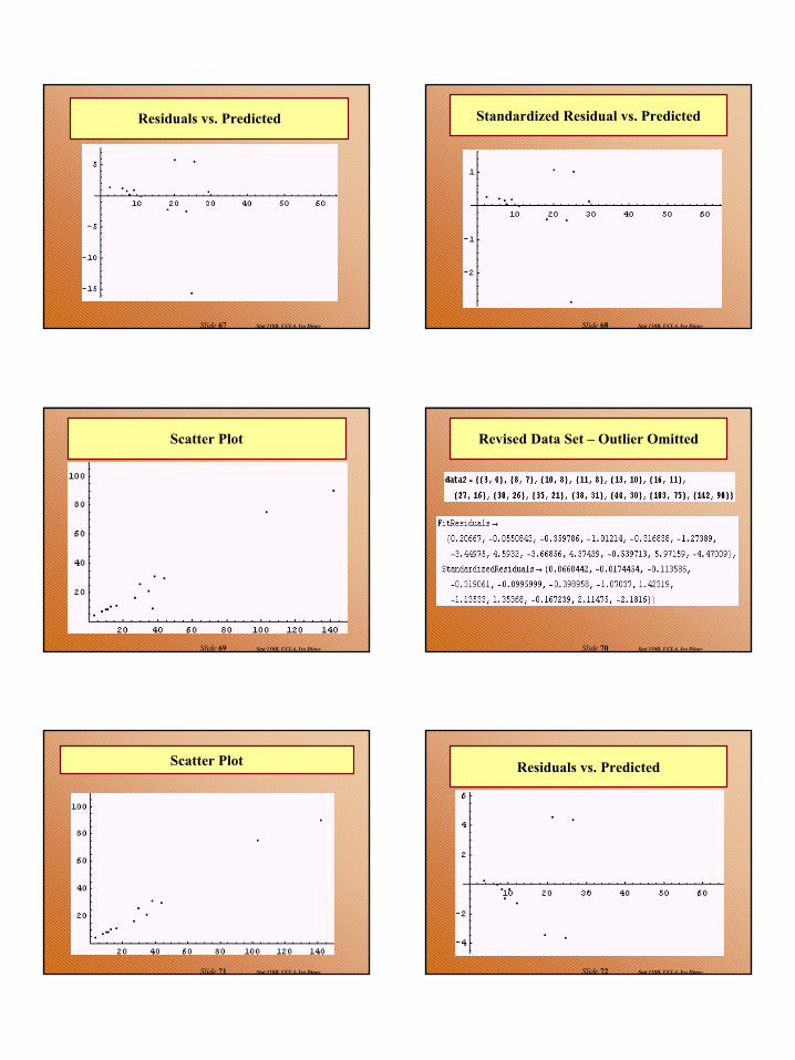
• The residuals support linearity and equal variances, but one of the standardized residuals is much greater (less) than +2 (-2) –This point is an outlier. If an assignable cause for this point may be found, throw it out and recalculate the regression parameters. If no assignable cause may be found, a MAD (minimum absolute deviation) approach may be used in place of L.S. (Least Squares). This approach, however, may be tedious.
Stat 110B, UCLA, Ivo DinovSlide 65
• A plot of the residuals vs. time show a violation of the independence assumption –A transformation may be used (if possible) or the time variable may be included in the model via multiple regression. See Applied Linear Regression Models.
• A plot of the residuals vs. an independent variable not included in the model exhibits a definite pattern – Include this independent variable in a multiple regression analysis
Stat 110B, UCLA, Ivo DinovSlide 66
Example: (12.4) Cont’d
12
Stat 110B, UCLA, Ivo DinovSlide 67
Residuals vs. Predicted
Stat 110B, UCLA, Ivo DinovSlide 68
Standardized Residual vs. Predicted
Stat 110B, UCLA, Ivo DinovSlide 69
Scatter Plot
Stat 110B, UCLA, Ivo DinovSlide 70
Revised Data Set – Outlier Omitted
Stat 110B, UCLA, Ivo DinovSlide 71
Scatter Plot
Stat 110B, UCLA, Ivo DinovSlide 72
Residuals vs. Predicted

13
Stat 110B, UCLA, Ivo DinovSlide 73
Standardized Residuals vs. Predicted
Stat 110B, UCLA, Ivo DinovSlide 74
Multiple Regression
The objective of multiple regression is to build a probabilistic model that relates a dependent (response) variable y to more than one independent (predictor) variables xi
Example: A particular steel company uses multiple regression to relate the dependent variable y = strength of hardened steel (psi) to the independent variables x1= temperature of heat treatment (oC) and x2= length of time treatment was applied (hours)
Stat 110B, UCLA, Ivo DinovSlide 75
General Multiple Regression Model
εβββ ++++= kk xxY ...110
Mean Response:**
110,..., ...**1
kkxxY xxn
βββµ +++=⋅
Stat 110B, UCLA, Ivo DinovSlide 76
Two Variable Models
First Order Model:
εβββ +++= 22110 xxY
First Order Model with Interactions:
εββββ ++++= 21322110 xxxxY
Stat 110B, UCLA, Ivo DinovSlide 77
Two Variable Models Cont’d
Second Order Model:
εβββββ +++++= 224
21322110 xxxxY
Second Order Model with Interactions:
εββββββ ++++++= 215224
21322110 xxxxxxY
Stat 110B, UCLA, Ivo DinovSlide 78
Data from Multiple Regression Model:
n observations: (y1,x11,…,xk1), (y2,x12,…,xk2), … , (yn,x1n,…,xkn)
Estimation of β’s: Take partial derivatives of D wrt b0,…,bk to obtain k+1 equations with k+1 unknowns. The solution yields L.S. estimates of the β’s
[ ]∑=
+⋅⋅⋅++−=n
ikikioi xbxbbyD
1
211 )(
14
Stat 110B, UCLA, Ivo DinovSlide 79
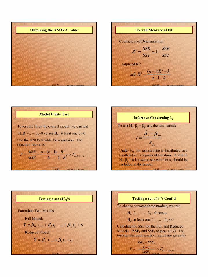
Obtaining the ANOVA Table
Stat 110B, UCLA, Ivo DinovSlide 80
Overall Measure of Fit
Coefficient of Determination:
SSTSSE
SSTSSRR −== 12
Adjusted R2:
knkRnRadj.
−−−−
=1)1(
22
Stat 110B, UCLA, Ivo DinovSlide 81
Model Utility Test
To test the fit of the overall model, we can test
Ho:β1=…= βk=0 versus Ha: at least one βj≠0
Use the ANOVA table for regression. The rejection region is
)1(,,2
2
1)1(
+−>−
+−== knkF
RR
kkn
MSEMSRF α
Stat 110B, UCLA, Ivo DinovSlide 82
Inference Concerning βj
To test Ho: βj = βjo use the test statistic
js
t jj
β
ββ
ˆ
0ˆ −
=
Under H0, this test statistic is distributed as a t with n-(k+1) degrees of freedom. A test of Ho: βj = 0 is used to see whether xj should be included in the model.
Stat 110B, UCLA, Ivo DinovSlide 83
Testing a set of βj’s
Formulate Two Models:
Full Model:
Reduced Model:
εβββ +++++= kkll xxY ......0
εββ +++= ll xY ...0
Stat 110B, UCLA, Ivo DinovSlide 84
Testing a set of βj’s Cont’d
To choose between these models, we test
Ho: βl+1=…= βk= 0 versus
Ha: at least one βl+1 ,…, βk ≠ 0
Calculate the SSE for the Full and Reduced Models. (SSEk and SSEl respectively). The test statistic and rejection region are given by
)1(,, +−−>−−
= knlkk
kl
FMSE
lkSSESSE
F α

15
Stat 110B, UCLA, Ivo DinovSlide 85
Confidence Intervals for the parameters βjand the mean response , and Prediction Intervals for future Y at x=x* are calculated in the usual manner. Consult page 583 of the text for the specific form of these intervals.
**1 ,..., nxxY ⋅
µ
Stat 110B, UCLA, Ivo DinovSlide 86
Picking a Regression Model – Variable Selection
1. Use Scientific Knowledge of the Problem
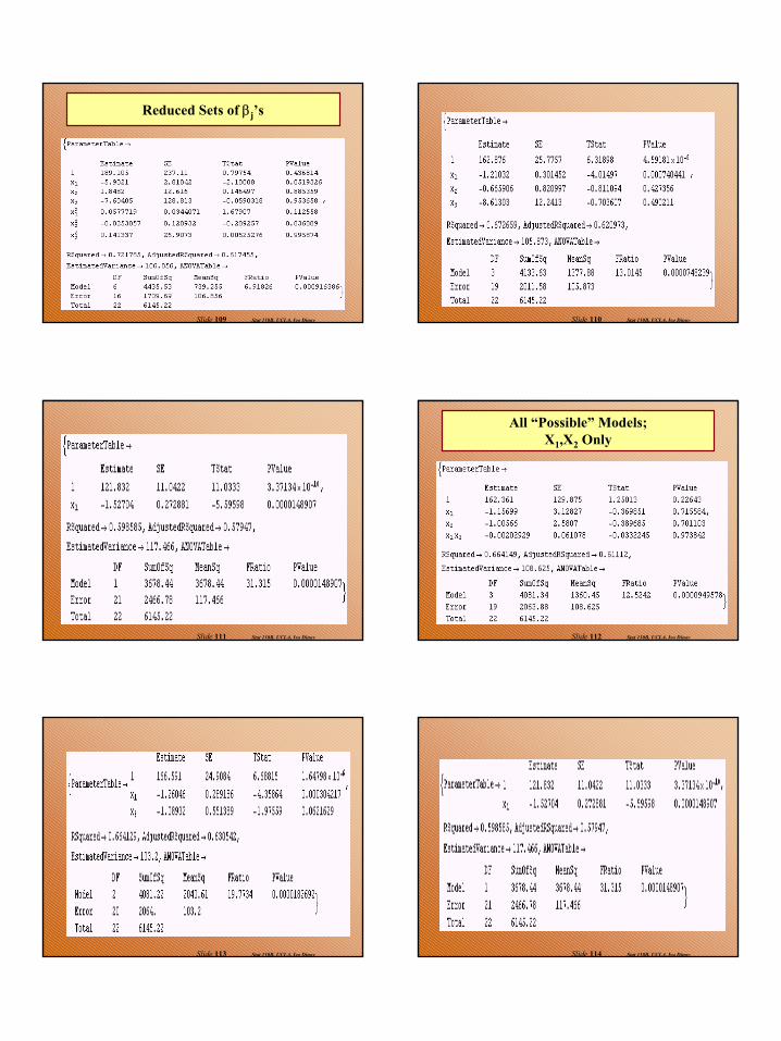
2. (Full Enumeration) Use a summary measure of fit on a possible regression models (R2, adj.R2, and SSE). Select the model with the “best” measures comparatively.
Stat 110B, UCLA, Ivo DinovSlide 87
3. (Backward Selection) Fit a model with all possible predictors included. Use t-tests for Ho: βj = 0 to suggest candidate xjpredictors to omit. Eliminate the “least significant” predictor and fit a new model. Continue until all variables are needed. Note: One cannot eliminate more than one variable at a time on this basis
Stat 110B, UCLA, Ivo DinovSlide 88
3. (Forward Selection) Build a model starting with the predictor most highly correlated with the response. Then find the best two-predictor model including this predictor, and so forth
Stat 110B, UCLA, Ivo DinovSlide 89
Multicollinearity
Multicollinearity among the predictor variables is said to exist when these variables are highly correlated amongst themselves.
Effects of Multicollinearity:
1. In general, data that exhibits multicollinearity does not inhibit our ability to obtain a good fit or affect inferences about the mean response and future observation
Stat 110B, UCLA, Ivo DinovSlide 90
2. In the presence of multicollinearity, The information obtained about the regression parameters, however, is imprecise. Hence the usual interpretation about these parameters in unwarranted (i.e. the effect of varying one parameter while holding the others constant).
Consult “Applied Linear Regression Models” for a detailed discussion of multicollinearity and possible remedies.
16
Stat 110B, UCLA, Ivo DinovSlide 91
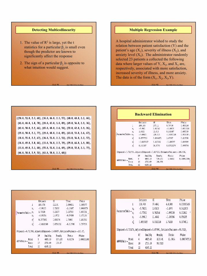
Detecting Multicollinearity
1. The value of R2 is large, yet the t statistics for a particular βj is small even though the predictor are known to significantly affect the response
2. The sign of a particular βj is opposite to what intuition would suggest.
Stat 110B, UCLA, Ivo DinovSlide 92
Multiple Regression Example
A hospital administrator wished to study the relation between patient satisfaction (Y) and the patient’s age (X1), severity of illness (X2), and anxiety level (X3). The administrator randomly selected 23 patients a collected the following data where larger values of Y, X2, and X3 are, respectively, associated with more satisfaction, increased severity of illness, and more anxiety. The data is of the form (X1, X2, X3,Y).
Stat 110B, UCLA, Ivo DinovSlide 93 Stat 110B, UCLA, Ivo DinovSlide 94
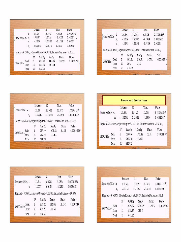
Backward Elimination
Stat 110B, UCLA, Ivo DinovSlide 95 Stat 110B, UCLA, Ivo DinovSlide 96
17
Stat 110B, UCLA, Ivo DinovSlide 97 Stat 110B, UCLA, Ivo DinovSlide 98
Stat 110B, UCLA, Ivo DinovSlide 99 Stat 110B, UCLA, Ivo DinovSlide 100
Forward Selection
Stat 110B, UCLA, Ivo DinovSlide 101 Stat 110B, UCLA, Ivo DinovSlide 102
18
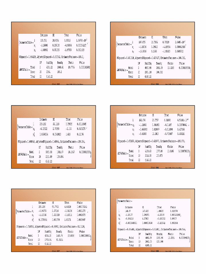
Stat 110B, UCLA, Ivo DinovSlide 103 Stat 110B, UCLA, Ivo DinovSlide 104
Stat 110B, UCLA, Ivo DinovSlide 105 Stat 110B, UCLA, Ivo DinovSlide 106
Stat 110B, UCLA, Ivo DinovSlide 107 Stat 110B, UCLA, Ivo DinovSlide 108
19
Stat 110B, UCLA, Ivo DinovSlide 109
Reduced Sets of βj’s
Stat 110B, UCLA, Ivo DinovSlide 110
Stat 110B, UCLA, Ivo DinovSlide 111 Stat 110B, UCLA, Ivo DinovSlide 112
All “Possible” Models; X1,X2 Only
Stat 110B, UCLA, Ivo DinovSlide 113 Stat 110B, UCLA, Ivo DinovSlide 114

20
Stat 110B, UCLA, Ivo DinovSlide 115 Stat 110B, UCLA, Ivo DinovSlide 116
Multicollinearity Example
The following data is a portion of that from a study of the relation of the amount of body fat (Y) to the predictor variables (X1) Tricep skinfold thickness, (X2) Thigh circumference, and (X3) Midarm circumference based on a sample of 20 healthy females 25-34 years old.
Stat 110B, UCLA, Ivo DinovSlide 117
Subject Triceps Thigh Midarm Body Fat1 19.5 43.1 29.1 11.92 24.7 49.8 28.2 22.83 30.7 51.9 37 18.7… … … … …18 30.2 58.6 24.6 25.419 22.7 48.2 27.1 14.820 25.2 51 27.5 21.1
Stat 110B, UCLA, Ivo DinovSlide 118
The L.S. regression coefficients for X1 and X2of various models are given in the table
Variables in Model b1 b2X1 0.8572 …X2 … 0.8565
X1, X2 0.224 0.6594X1, X2, X3 4.334 -2.857
Stat 110B, UCLA, Ivo DinovSlide 119
Hence, the regression coefficient of one variable depends upon which other variables are in the model and which ones are not. Therefore, a regression coefficient does not reflect any inherent effect of particular predictor variable on the response variable (Only a partial effect, given what other variables are included)