ultimate dance party - carnegie mellon universityee551/projects/f08/g2_final...of course, the...

ULTIMATE DANCE PARTY

Final Report 18-551 Fall 2008

Group 2

Yang Zhou ([email protected]) Tina Milo ([email protected])

David Tuzman ([email protected])

18-551: Group 2, Fall 2008 Ultimate Dance Party

of 2

TABLE OF CONTENTS 1 Project Explanation...................................................................................................4

1.1 Problem ...............................................................................................................4 1.2 Solution ...............................................................................................................4 1.3 Initial Goals .........................................................................................................5

2 Prior Projects .............................................................................................................6 2.1 One Voice: Vocal Harmony Generator Fall 2006, Group 9................................6 2.2 Look Who’s Talking Fall 2007, Group 2 ............................................................7

3 Algorithms..................................................................................................................7 3.1 Beat Detection .....................................................................................................7 3.2 Phase Vocoder ...................................................................................................11

4 Obstacles Encountered............................................................................................16 4.1 Internal Memory Usage Issues ..........................................................................16 4.2 Speed Issues and Estimates ...............................................................................18 4.3 Effects on Sampling Rate and FFT size ............................................................21 4.4 Optimizations ....................................................................................................22 4.5 Page Alignment .................................................................................................22

5 Results/Demo ...........................................................................................................23 5.1 Signal Flow........................................................................................................23 5.2 Database ............................................................................................................24 5.3 Demo: what worked ..........................................................................................24 5.4 GUI....................................................................................................................27

6 Additional Work......................................................................................................29 7 Schedule/Who Did What.........................................................................................30 8 Future Work ............................................................................................................31

8.1 Using FastRTS ..................................................................................................31 8.2 Get 8kHz codec playback to work ....................................................................32 8.3 Workout page alignment ...................................................................................32

9 Additional References .............................................................................................33


of 3

TABLE OF FIGURES Figure 1: Initial Beat Detection Diagram ............................................................................8 Figure 2: Final Beat Detection Diagram ...........................................................................10 Figure 3: STFT Example...................................................................................................11 Figure 4: Magnitude Interpolation ....................................................................................12 Figure 5: Phase Accumulation ..........................................................................................13 Figure 6: ISTFT Example..................................................................................................14 Figure 7: Libraries Used....................................................................................................18 Figure 8: Cycle times for various math functions on the DSK .........................................19 Figure 9: System Diagram.................................................................................................23 Figure 10: DSK and PC Data Flow ...................................................................................24 Figure 11: Original Spectrogram.......................................................................................25 Figure 12: Spectrogram with r = 1 ....................................................................................26 Figure 13: Spectrogram with r = 2 ....................................................................................26 Figure 14: Main GUI Screen .............................................................................................27 Figure 15: Progress Bar for Beat Detection ......................................................................28 Figure 16: Dialog box for sending song to DSK...............................................................28 Figure 17: Entertainment while phase vocoder is processing ...........................................28 Table 1: Beat Detection versus Pitch Detection..................................................................6 Table 2: DSK memory configuration excerpt from map file (in bytes) ............................17 Table 3: Memory Used and Page Size Correlation ...........................................................17 Table 4: Values of variables in the phase vocoder algorithm ...........................................18 Table 5: STFT Estimate ....................................................................................................20 Table 6: ISTFT Estimate ...................................................................................................20 Table 7: Observed Cycles..................................................................................................22 Table 8: Cycles after Optimization ...................................................................................29 Table 9: Schedule ..............................................................................................................30 Table 10: STFT Estimate using FastRTS..........................................................................31 Table 11: ISTFT Estimate using FastRTS ........................................................................31 Table 12: Total Estimates for Phase Vocoder using FastRTS ..........................................32


of 4

1 Project Explanation

1.1 Problem The problem we are addressing is called beat synchronization. Beat

synchronization refers to the process of first detecting the number of beats per minute (also known as the tempo) of a given recorded song or clip of music, and then modifying that tempo to match another desired tempo. However, simply altering the playback speed introduces unwanted effects in pitch (think of playing a 33 rpm vinyl record at 45 rpm), and it is therefore desirable to perform beat synchronization without affecting the frequency characteristics of the original song. Beat synchronization is common and extremely useful in modern music processing. For example there are many software-based products (such as Ableton Live or Digidesign “X-form” plug-in) that perform beat synchronization for music playback and computer music composition, but not any well-known hardware implementations. Other possible applications include slowing down speech (while otherwise minimally effecting the signal) for increased intelligibility, and, of course, the ultimate dance party, in which many songs can be normalized to one tempo and then strung together to provide maximum grooveability.

1.2 Solution Our project aims to automate the beat synchronization process. In other words, an

input song can be manipulated to have a desired tempo, or two input songs can be manipulated to have the same tempo. Most modern popular music has envelope peaks repeated in time with the tempo of the song. Using this assumption, we find peak patterns in the input data (the song). In order to separate different instruments in the recording, we analyze the input song using filter banks and search for patterns within groups of frequencies (loosely distinguishing drums/guitar/bass/vocals). We then perform time-scaling to change the bpm. Our project not only performs automatic beat synchronization of two songs, but also allows for user-defined time scaling of one input song.


of 5

1.3 Initial Goals

The signal to be processed will be professionally recorded music that has a static tempo. We will only analyze 2 seconds from the middle of the song for beat detection. The sampling frequency should optimally be 44.1 kHz to capture the entire bandwidth of the audio range: 20 Hz to 20 kHz. After initial calculations we chose an acceptable sampling rate of 22.050 kHz, however, we later had to reduce the sampling rate to improve efficiency. This will be detailed in the “Computations” section. For the beat detection component of our project, we will implement the algorithm developed in “Beat This”1, a project from Rice University. “Beat This” utilizes functions in MATLAB in order to detect a beat in a song. The MATLAB code for the beat detection algorithm is published and is tailored to run on a PC. We plan to combine the algorithm developed in this project with an algorithm constructed using wavelets2. We will first implement our combined algorithm in MATLAB code and then develop C code. In addition, we will need to implement code to change the tempo of a song, while maintaining its pitch, to match the beat detected earlier. We will use a Phase Vocoder3 algorithm to implement this change.

The database that the DSK will use will be a group of 50 songs, residing on the

PC. The DSK will take two songs as inputs: one song will have the target beat and the other song will be changed to have the beat as the first. We will perform beat detection, apply the phase vocoder, and the output from the DSK will be the new song playing in real time with a changed beat.

1 http://www.owlnet.rice.edu/~elec301/Projects01/beat_sync/beatalgo.html 2 http://soundlab.cs.princeton.edu/publications/2001_amta_aadwt.pdf 3 http://www.panix.com/~jens/pvoc‐dolson.par


of 6

2 Prior Projects

2.1 One Voice: Vocal Harmony Generator Fall 2006, Group 9 This project focused on pitch detection and pitch scaling, which is similar to our

focus of beat detection and time scaling. Their pitch detection algorithm started similarly by attempting to discover the periodicity of the signal through autocorrelation. Our strategy first split the signal into multiple filter banks and analyzed them separately since our input is composed of multiple fundamental tones; One Voice separated the unvoiced and voiced parts of speech and only analyzed the voiced parts. Both of our initial algorithms used multiple smoothing filters followed by autocorrelation. After this, both of our algorithms attempted to detect the periodicity of the signal (in their project periodicity = pitch; in our project periodicity = tempo). Both of our projects found the autocorrelation to be difficult to adapt to a robust algorithm applicable to various signals without individual tweaking for each, and we both decided to choose a varying comb filter in replacement of the autocorrelation (Carpentier algorithm).

The pitch scaling part of One Voice also is similar to the time scaling (phase vocoder) part of our project. Their algorithm manually detects peaks in the time domain throughout the song (wavelength follows pitch) and synthesizes them into a new signal through overlap-add, mapping detected peaks to new peak positions to scale the pitch (Pitch Synchronous OverLap-Add). Since our input signal is composed of many more frequencies, we use an STFT to estimate the magnitudes of multiple (N/2) frequencies. This estimation is compensated in our phase reconstruction, which also suppresses the noise caused by overlap-add process of PSOLA.

In short, One Voice pitch scales strictly in the time domain, precisely detecting single periodicities, and constructing result through overlap-add; Ultimate Dance Party pitch/time scales in a frequency domain (STFT), approximating multiple periodicities, and reconstructing through magnitude interpolation and phase accumulation.

2.1.1 Beat detection vs. pitch detection Beat detection and pitch detection are similar processes, since they both detect the

frequency of a signal. The human ear interprets audio as a beat (impulse) or a Tone depending on the signal’s frequency, thus determining the range of frequencies each algorithm will find: Beat Detection Pitch Detection What your ear hears: Beat / Impulse Tone Range in Hz (cyc/sec) 0 – 20 20 – 20,000 Range in BPM (cyc/min) 0 – 1,200 1,200 – 1,200,000

Table 1: Beat Detection versus Pitch Detection


of 7

2.2 Look Who’s Talking Fall 2007, Group 2 This project’s aim was to detect certain words spoken from a voice source. The

project involved training through Dynamic Time Warping to account for different speeds of speech. Through completing their project, they discovered Dan Ellis’s A Phase Vocoder in MatLab and commented that it is a superior algorithm for time shifting due to its clever way of magnitude interpolation. We have taken their advice and used his algorithm as a starting point in our project.

3 Algorithms

3.1 Beat Detection

3.1.1 Initial Desired Beat Detection Algorithm

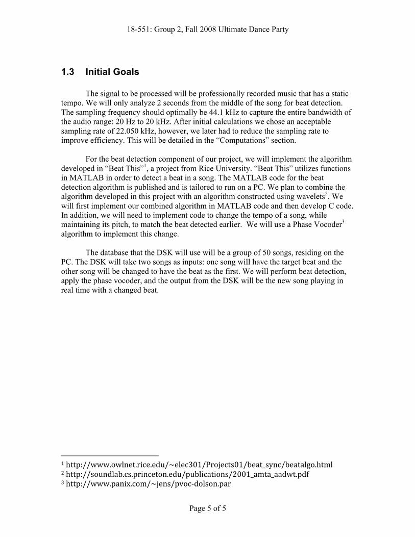
Our initial beat detection algorithm works as follows: a 2 second segment is extracted from the input song, and passed through a filter bank so that different instrument groups (bass, treble etc) are divided into frequency bands and can therefore be analyzed separately. Then for each frequency band, the signal is smoothed with a Hamming window to extract the envelope of the signal, and then differentiated to emphasize the change in the envelope. Then half-wave rectification is performed and the resulting signals are summed together. The goal of this is to obtain a signal with more salient beats so that the autocorrelation of this signal will produce distinct periodic peaks corresponding to each beat. We will then calculate the tempo based on the period of these peaks, repeat the whole process for other 2 second segments, and average the calculated tempos to obtain our final detected tempo.


of 8

Figure 1: Initial Beat Detection Diagram


of 9

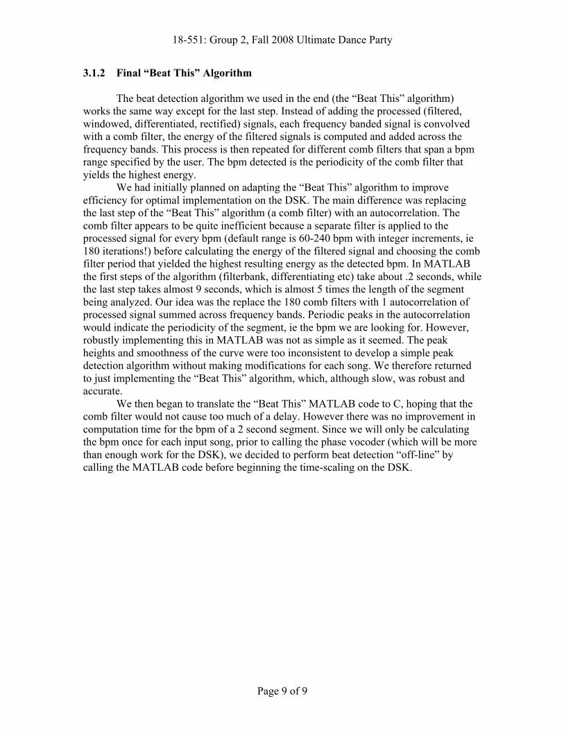
3.1.2 Final “Beat This” Algorithm

The beat detection algorithm we used in the end (the “Beat This” algorithm) works the same way except for the last step. Instead of adding the processed (filtered, windowed, differentiated, rectified) signals, each frequency banded signal is convolved with a comb filter, the energy of the filtered signals is computed and added across the frequency bands. This process is then repeated for different comb filters that span a bpm range specified by the user. The bpm detected is the periodicity of the comb filter that yields the highest energy.

We had initially planned on adapting the “Beat This” algorithm to improve efficiency for optimal implementation on the DSK. The main difference was replacing the last step of the “Beat This” algorithm (a comb filter) with an autocorrelation. The comb filter appears to be quite inefficient because a separate filter is applied to the processed signal for every bpm (default range is 60-240 bpm with integer increments, ie 180 iterations!) before calculating the energy of the filtered signal and choosing the comb filter period that yielded the highest resulting energy as the detected bpm. In MATLAB the first steps of the algorithm (filterbank, differentiating etc) take about .2 seconds, while the last step takes almost 9 seconds, which is almost 5 times the length of the segment being analyzed. Our idea was the replace the 180 comb filters with 1 autocorrelation of processed signal summed across frequency bands. Periodic peaks in the autocorrelation would indicate the periodicity of the segment, ie the bpm we are looking for. However, robustly implementing this in MATLAB was not as simple as it seemed. The peak heights and smoothness of the curve were too inconsistent to develop a simple peak detection algorithm without making modifications for each song. We therefore returned to just implementing the “Beat This” algorithm, which, although slow, was robust and accurate.

We then began to translate the “Beat This” MATLAB code to C, hoping that the comb filter would not cause too much of a delay. However there was no improvement in computation time for the bpm of a 2 second segment. Since we will only be calculating the bpm once for each input song, prior to calling the phase vocoder (which will be more than enough work for the DSK), we decided to perform beat detection “off-line” by calling the MATLAB code before beginning the time-scaling on the DSK.


of 10

Figure 2: Final Beat Detection Diagram


of 11

3.2 Phase Vocoder The Phase Vocoder algorithm begins with a Short Time Fourier Transform. This captures the frequency spectrum as it changes in time. In our implementation, N = 512 and Hop = 128: A) Take N-size sections of the original signal. The start/end points of each section are offset by Hop. When Hop is smaller than N, the STFT retains faster changes in the frequency spectrum. B) Multiply the each section by a Hamming window in order to suppress side lobes in the frequency spectrum C) Perform N-point FFT on each of the windowed sections. The magnitudes and phases are stored in columns of separate matrixes. In this way, progressing through a column of the FFT (Mag or Phase) matrix will relate to the FFT of the original samples: {Hop*Col#, Hop*Col# + N} For N = 512, Hop = 128 (as we use), and original signal length = 2048 (for example), the first few columns represent:{0 through 511} {128 through 639} {256 through 767} {384 through 895} …and the last few columns: {1152 through 1663} {1280 through 1791} {1408 through 1919}

Figure 3: STFT Example {1536 through 2047} Total Number of Columns = (length – N)/Hop + 1 = 13 Columns Note: We choose “length” so that (length – N)/Hop is an integer

Short Time Fourier Transform Example N = 512, Hop = 256… 3 iterations


of 12

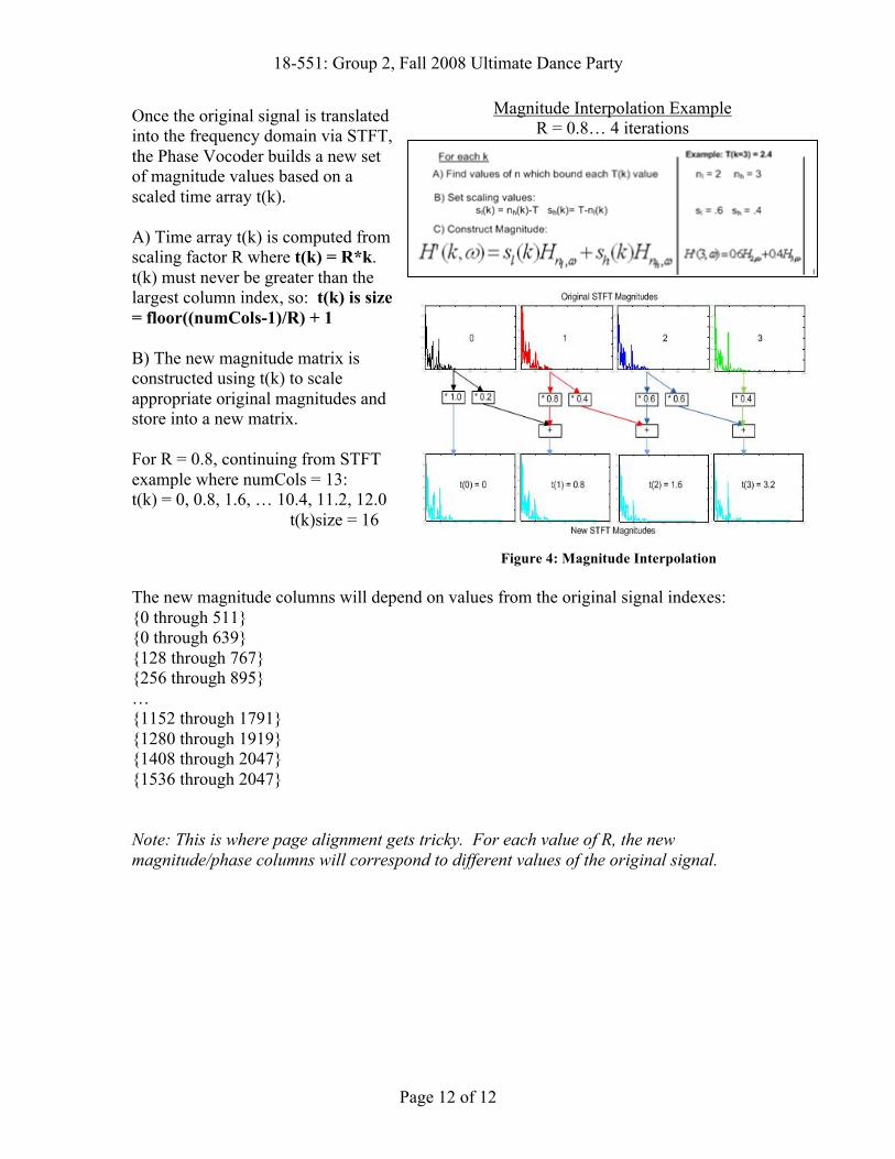
Once the original signal is translated into the frequency domain via STFT, the Phase Vocoder builds a new set of magnitude values based on a scaled time array t(k). A) Time array t(k) is computed from scaling factor R where t(k) = R*k. t(k) must never be greater than the largest column index, so: t(k) is size = floor((numCols-1)/R) + 1 B) The new magnitude matrix is constructed using t(k) to scale appropriate original magnitudes and store into a new matrix. For R = 0.8, continuing from STFT example where numCols = 13: t(k) = 0, 0.8, 1.6, … 10.4, 11.2, 12.0

t(k)size = 16

Figure 4: Magnitude Interpolation The new magnitude columns will depend on values from the original signal indexes: {0 through 511} {0 through 639} {128 through 767} {256 through 895} … {1152 through 1791} {1280 through 1919} {1408 through 2047} {1536 through 2047} Note: This is where page alignment gets tricky. For each value of R, the new magnitude/phase columns will correspond to different values of the original signal.

Magnitude Interpolation Example R = 0.8… 4 iterations


of 13

In order to construct the new phase matrix, the Phase Vocoder first computes the expected phase advance dphi(n) of each bin: dphi(n) = 2πHop*n / N. This is the phase advance you would see from a sinusoid at the center frequency of a bin in an N point FFT if you shifted the input window by Hop points. This is used to estimate the frequency of a sinusoid that makes the phase difference observed in the original phase matrix. Note: This is only necessary when the STFT and iSTFT have different Hop sizes. In our implementation, the Hop size is constant. We did not realize this until the end of our project. In the code, dphi(n) is simply added and then subtracted from the final phase, rendering it pointless. To start accumulating the phase, the phase of the first new column is set equal to the phase of the old new column. Then, using the same bounds and t(k) as the Magnitude Interpolation, the phase difference between respective original column is added to the current phase values.

Figure 5: Phase Accumulation The new STFT Phase columns depend on the same indexes from the original signal as the new STFT Magnitude columns (refer to prior page).

Phase Accumulation Example R = 1.2… 3 iterations


of 14

Finally, the iSTFT is performed: A) The new phase and magnitude values are converted in rectangular coordinates. N-point iFFT is performed on each section, and the result is Hamming windowed. B) The resulting sections are each offset accordingly (Offset(k) = Hop*k) and summed in order to produce the final output. C) Except for the first and last group of samples of the final output, each sample is the sum of four values. The first and last N-Hop samples (384 in our case) do not have enough overlapping iFFTs to sum similarly, thus they are inaccurately scaled and useless.

Figure 6: ISTFT Example t(0) depends on original signal values of indexes {0 through 511} t(1) depends on original signal values of indexes {0 through 629} t(2) depends on original signal values of indexes {128 through 767} t(3) depends on original signal values of indexes {256 through 895} t(4) depends on original signal values of indexes {384 through 1023} t(5) depends on original signal values of indexes {512 through 1151} t(6) depends on original signal values of indexes {512 through 1151} Values summed between the beginning and end of t(4) are accurate, therefore the original signal was accurately solved for indexes {384 through 1023}, leaving unsolved values of size 384 at the beginning of the input and the of size 128 at the end of the input. Note: While deriving this algorithm earlier, we wrongly found that the number of useless values on each side of the output was equal to N. We did not find our error until after the presentation and demo.

Inverse Short Time Fourier Transform Example R = 0.8, N = 512, Hop = 128… 7 iterations


of 15

3.2.1 Page Alignment

In Dan Ellis’s MatLab Phase Vocoder algorithm, the STFT for the entire song is executed at once. This causes only two cases of inaccurate output values (edge errors). Since these values are at the beginning and end of the song, which normally contains silence or near silence, the effect of these errors is negligible. In our DSK implementation, we perform the STFT of multiple input pages (splices) of the song. This causes the edge errors to occur multiple times in the output. In addition to this, all the pages must be concatenated together smoothly. This requires the end of one page to align perfectly with the beginning of the next page. If the pages are not aligned properly, there will be audible distortion in the output. Note: The following derivation is INCORRECT. This is what we were using at the time of the presentation and demo. The equations were found through using multiple values of R, finding their appropriate values, and then constructing equations which solved for all values of R. This derivation uses N = 512 and Hop = 128, Scaling factor = R.

Assuming the output of each page has 512 useless values in the beginning and 512+384=896 in the end, we must pad the input with more values accordingly. In order to solve how much padding is necessary, we will start from the output. The useless values in the output correspond to the first and last 4 columns of the new STFT. The original STFT values that correspond to the useless output depend on R as such:

Front columns floor(4*R) and lower are not solved for correctly End columns ceil((numCols – 5)*R) and higher are not solved for correctly

The useless columns in the original STFT matrix correspond to unsolved indexes in the original signal. This correspondence does not depend on R besides the column values:

Front indexes Hop*floor(4*R) - 1 and lower are not solved for correctly End indexes Hop*ceil((numCols – 5)*R) and higher are not solved for correctly

This results in Hop*floor(4*R) error-prone values the beginning of the page and Hop*floor(4*R) + 384 error-prone values in the end of the page. We chose to have a constant 2048 non-error-prone values between these values. To account for the error-prone values, each input page is offset from its neighbor by only 2048, rather than entire page length.

Note: We have not yet derived an accurate padding scheme. Some things we know are incorrect in our derivation is the assumption of useless values in the output and the conversion of the highest accurate original STFT column and the highest non-error-prone index.


of 16

4 Obstacles Encountered During the course of development we run into a variety of issues which hindered

the successful transition of the phase vocoder from C code on the PC to C code on the DSK. The main obstacles that we encountered related to storage, speed, paging, and code optimization.

4.1 Internal Memory Usage Issues In order to ensure that memory accesses would not bog down our computations,

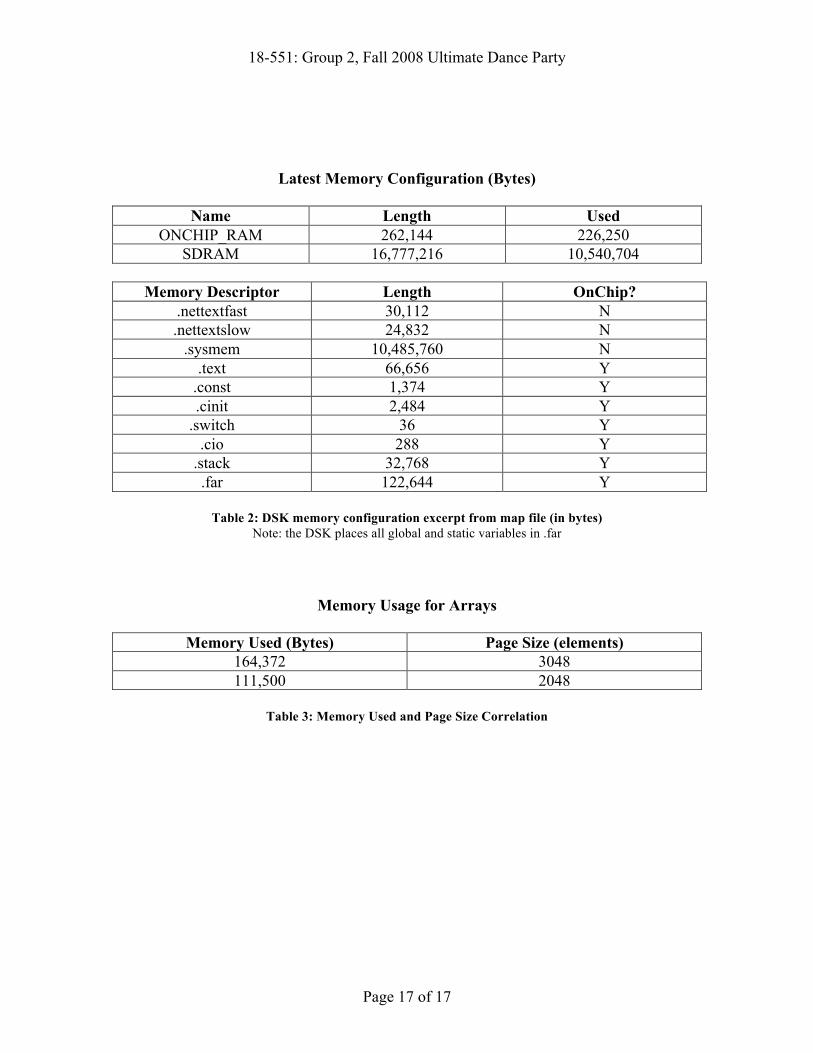
we determined that all of the arrays needed for the phase vocoder needed to be on the DSK in internal memory. However, during the initial phases of the transition between PC code and DSK code, we found out that there was not enough internal memory to store the arrays needed for the phase vocoder. Our previous estimates for storage requirements were incorrect because we did not take into account additional internal memory storage that is not a product of the phase vocoder.

Storage elements that we did not take into account were the code size (.text) and DSK network code from net.lib (.nettextfast and .nettextslow). The code size for our project ended up taking approximately 66,656 bytes and code from net.lib 54,944 bytes. Refer to Table x for more information. Thus code alone took up 121,600 bytes and since the DSK has only about 260 KB of internal memory this left only 103,500 bytes for our phase vocoder arrays (after taking into account all other memory usages). In order to maximize the amount of storage available for the algorithm, we had to evict sections of code from internal memory and place them in external memory. We tried to place .text in external memory but that drastically increased execution time. Because the PC->DSK transfer is only done in the beginning before the start of the algorithm, we moved net.lib from internal to external memory as this would not impact the execution time of the phase vocoder. Although this freed up much needed memory, everything still did not fit. We then proceeded to reduce the page size from 3048 samples to 2048 samples. Thus we finally had the room necessary to perform the phase vocoder entirely in internal memory. Refer to Table x+1 for additional information about page size and total memory needed. The scaling factor is directly proportional to the amount of memory needed to store the phase vocoder arrays. As scaling factor increases, the amount of memory needed also increases. This is because additional padding is needed during paging to compensate for the unusable portions of the output at the beginning and at the end. For more information about the phase vocoder please refer to the phase vocoder section of this document. The code that we have written can accommodate a song with a maximum scaling factor of 3.0.


of 17

Latest Memory Configuration (Bytes)

Name Length Used ONCHIP_RAM 262,144 226,250

SDRAM 16,777,216 10,540,704

Memory Descriptor Length OnChip? .nettextfast 30,112 N .nettextslow 24,832 N

.sysmem 10,485,760 N .text 66,656 Y

.const 1,374 Y .cinit 2,484 Y

.switch 36 Y .cio 288 Y

.stack 32,768 Y .far 122,644 Y

Table 2: DSK memory configuration excerpt from map file (in bytes)

Note: the DSK places all global and static variables in .far

Memory Usage for Arrays

Memory Used (Bytes) Page Size (elements) 164,372 3048 111,500 2048

Table 3: Memory Used and Page Size Correlation


of 18

Figure 7: Libraries Used

4.2 Speed Issues and Estimates

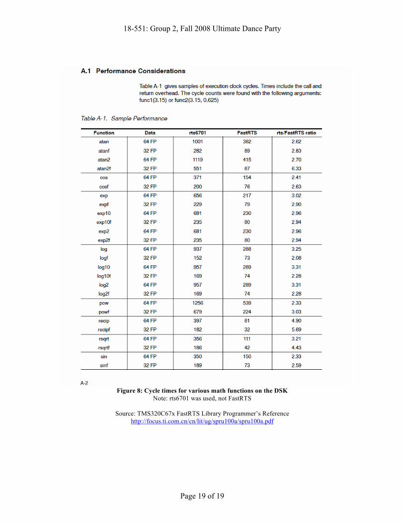
We ran into a major problem after handling our storage issues. We found that even with all of our arrays stored in internal memory the DSK still did not run the phase vocoder algorithm correctly for our real-time implementation. More specifically, the buffer storing the processed contents was being played twice by the codec. This implies that the output buffer was not getting refreshed with processed data quickly enough. After careful analysis, we found that the initial timing estimates computed for the phase vocoder algorithm were inaccurate . We did not account for the processing time it would take to execute math functions such as cosf, powf, sinf and atan2f. In addition, the paging process introduced additional code and made computation slower than was estimated. Another important variable that we did not account for was the fact that the arguments for fftn.c (the fft function used in the C implementation of the phase vocoder algorithm on the PC) were very different from the fft functions we used on the DSK. The fft functions used on the DSK needed real and imaginary data to be interleaved into one array whereas fftn.c took separate arrays for real and imaginary data. Thus, a process of interleaving and de-interleaving data had to be introduced making our code longer and adding additional computations / memory accesses. Out of all of the new code that was introduced into the DSK phase vocoder, the critical elements were found to be loops containing math functions. These math functions increased the cycle time for each function considerably. The most notable computation that took the longest amount of time was the calculation of the magnitude and phase during the STFT part of the phase vocoder algorithm. This calculation took 3 powf calls and one tan2f call for each pair of output from the FFT. During each paging process the FFT was called 13 times and for each FFT output, 256 magnitude and phase calculations had to be performed. The following is a delineation of how the speed estimates were calculated. Refer to table 1 for values of variables which were helpful in estimating cycle times. Refer to figure 1 for average speeds of various math functions on the DSK.

Page Size: 2048 Number of Rows: 257 Number of Columns: 13

Table 4: Values of variables in the phase vocoder algorithm


of 19

Figure 8: Cycle times for various math functions on the DSK

Note: rts6701 was used, not FastRTS

Source: TMS320C67x FastRTS Library Programmer’s Reference http://focus.ti.com.cn/cn/lit/ug/spru100a/spru100a.pdf


of 20

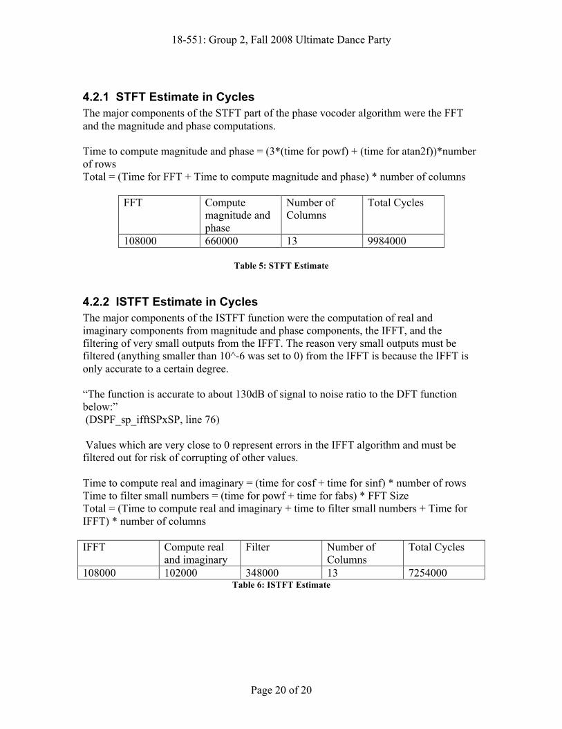
4.2.1 STFT Estimate in Cycles The major components of the STFT part of the phase vocoder algorithm were the FFT and the magnitude and phase computations. Time to compute magnitude and phase = (3*(time for powf) + (time for atan2f))*number of rows Total = (Time for FFT + Time to compute magnitude and phase) * number of columns

FFT Compute magnitude and phase

Number of Columns

Total Cycles

108000 660000 13 9984000

Table 5: STFT Estimate

4.2.2 ISTFT Estimate in Cycles The major components of the ISTFT function were the computation of real and imaginary components from magnitude and phase components, the IFFT, and the filtering of very small outputs from the IFFT. The reason very small outputs must be filtered (anything smaller than 10^-6 was set to 0) from the IFFT is because the IFFT is only accurate to a certain degree. “The function is accurate to about 130dB of signal to noise ratio to the DFT function below:” (DSPF_sp_ifftSPxSP, line 76) Values which are very close to 0 represent errors in the IFFT algorithm and must be filtered out for risk of corrupting of other values. Time to compute real and imaginary = (time for cosf + time for sinf) * number of rows Time to filter small numbers = (time for powf + time for fabs) * FFT Size Total = (Time to compute real and imaginary + time to filter small numbers + Time for IFFT) * number of columns IFFT Compute real

and imaginary Filter Number of

Columns Total Cycles

108000 102000 348000 13 7254000 Table 6: ISTFT Estimate


of 21

4.2.3 PVSample Estimate in Cycles Computing the timing estimate for PVSample is quite difficult. The floor function

was used 5 times in a loop that iterates 6144 times. In addition, much of the computation inside PVSample involved floating point multiplication which usually takes more than one cycle, and the number of cycles it will take is hard to predict. This number is not known and can fluctuate depending on the values of each factor in the multiply.

4.3 Effects on Sampling Rate and FFT size Based on our initial calculations, we decided the DSK could support our

algorithm using a sampling rate of 22.050kHz and 1024-point FFTs. We wanted to use TI’s fast radix-4 ASM FFT code, but this code is not-interruptible and therefore incompatible with codec playback. We acquired a newer version of the same code which is interrupt tolerant, but disabling interrupts before FFTs and then enabling interrupts afterwards causing significant lags in playback. We finally used mixed-radix C code which is fully interruptible but slow for computations at 22.050kHz. According to the FFT documentation, the 512 ASM FFT should take about 10,000 cycles, but our C FFT function took about 95,000 samples (measured with profiling). We did not profile the ASM FFT, so we are not sure if the measured discrepancy would be this large. We then decreased the sampling rate to 16kHz, which improved the output quality slightly. We also changed our FFT size from 1024 to 512 because tests in MATLAB revealed that a higher FFT size (2048 at 22.050kHz and 1024 at 16kHz) introduced a reverb-like effect which is an unwanted distortion. Unfortunately, after these modifications, processing and playback at 16kHz was still slow, and the output sounded quite choppy and delayed (even with all significant variables crammed into internal memory). We then profiled our phase vocoder function (see table below) and determined that each page (1024 samples) was taking about .0991 seconds to process, which is a much longer than the time required to play one page (1024 samples at 16kHz = .064 seconds). Based on these calculations, we think our phase vocoder could work in real-time if the sampling rate were reduced to 8kHz since 1024 samples at 8kHz = .128 seconds, which is greater than the .0991 second computation time. We tried to make this adjustment, but did not have time to complete the changes and debugging.


of 22

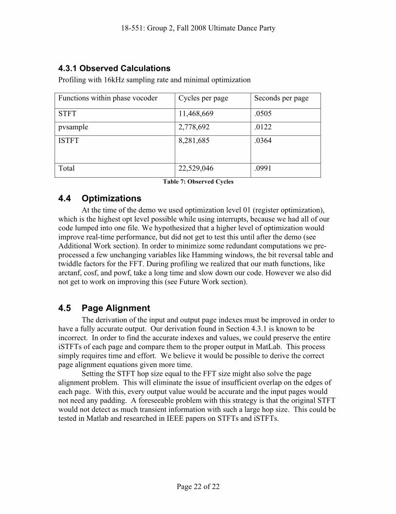
4.3.1 Observed Calculations Profiling with 16kHz sampling rate and minimal optimization Functions within phase vocoder Cycles per page Seconds per page

STFT 11,468,669 .0505

pvsample 2,778,692 .0122

ISTFT 8,281,685 .0364

Total 22,529,046 .0991

Table 7: Observed Cycles

4.4 Optimizations At the time of the demo we used optimization level 01 (register optimization),

which is the highest opt level possible while using interrupts, because we had all of our code lumped into one file. We hypothesized that a higher level of optimization would improve real-time performance, but did not get to test this until after the demo (see Additional Work section). In order to minimize some redundant computations we pre-processed a few unchanging variables like Hamming windows, the bit reversal table and twiddle factors for the FFT. During profiling we realized that our math functions, like arctanf, cosf, and powf, take a long time and slow down our code. However we also did not get to work on improving this (see Future Work section).

4.5 Page Alignment The derivation of the input and output page indexes must be improved in order to have a fully accurate output. Our derivation found in Section 4.3.1 is known to be incorrect. In order to find the accurate indexes and values, we could preserve the entire iSTFTs of each page and compare them to the proper output in MatLab. This process simply requires time and effort. We believe it would be possible to derive the correct page alignment equations given more time. Setting the STFT hop size equal to the FFT size might also solve the page alignment problem. This will eliminate the issue of insufficient overlap on the edges of each page. With this, every output value would be accurate and the input pages would not need any padding. A foreseeable problem with this strategy is that the original STFT would not detect as much transient information with such a large hop size. This could be tested in Matlab and researched in IEEE papers on STFTs and iSTFTs.


of 23

5 Results/Demo

5.1 Signal Flow

Below is an overview of our system and the dataflow between the PC and the DSK. Basically, the user either selects two input songs to beatmatch or selects one input song and a time scaling factor. For example, the user can pick a song and specify a scaling factor of 2 which indicates a desired output that is twice as fast as the original song. The input song, or song to be scaled is then transferred to the DSK and stored in external memory. Then chunks, or pages, of the song are paged into internal memory, processed with our phase vocoder, and played out through the codec while the next page is brought in and processed. Since we did not get our phase vocoder computations fast enough for real-time playback through the codec, we added the capability to send each processed paged back to the PC. Once the whole song is processed, all the pages are concatenated on the PC side, and the compiled output song can be played in MATLAB or another media player. In summary, the DSK stores the input song, handles paging, processes each page, and finally sends each processed block to the codec and to the PC. The PC read in the input files, performs the beat detection algorithm, hosts the GUI, sends the song, user inputs, and bpm to the DSK, and finally concatenates the DSK output chunks to create the final output song.

Figure 9: System Diagram

PC Audio Playback


of 24

Figure 10: DSK and PC Data Flow

5.2 Database Our database is segments of recorded music, wav files specifically. We planned to rip songs from various Billboard CD collections, but ended up using wav files from Sony Music website (pop and r&b songs), and converting them to 16kHz in MATLAB. For beat synchronization, we also assume that the song has a static tempo, which is generally true for pop music, but definitely not for classical music.

5.3 Demo: what worked For our demo, the user was able to select a file, and select a time-scaling factor for the input file in a slider in the GUI. Then the beat is detected, the song is processed, the output wav file is created from the output pages sent by the DSK, and the output is read in and played using MATLAB. As we mentioned above, we were not able to play the output in real-time from the DSK. Because of this, we were also unable to create a playback slider for the user to jump forward or backward in the song. Also, during the demo, we did not beat match two input files, but modifying our demo procedure for this is trivial. To evaluate the results of the phase vocoder, beat detection can be called on the output of the phase vocoder to verify the that new bpm is the product of the selected time scaling

7b. Send processed chunk to PC PC concatenates chunks for continuous play back


of 25

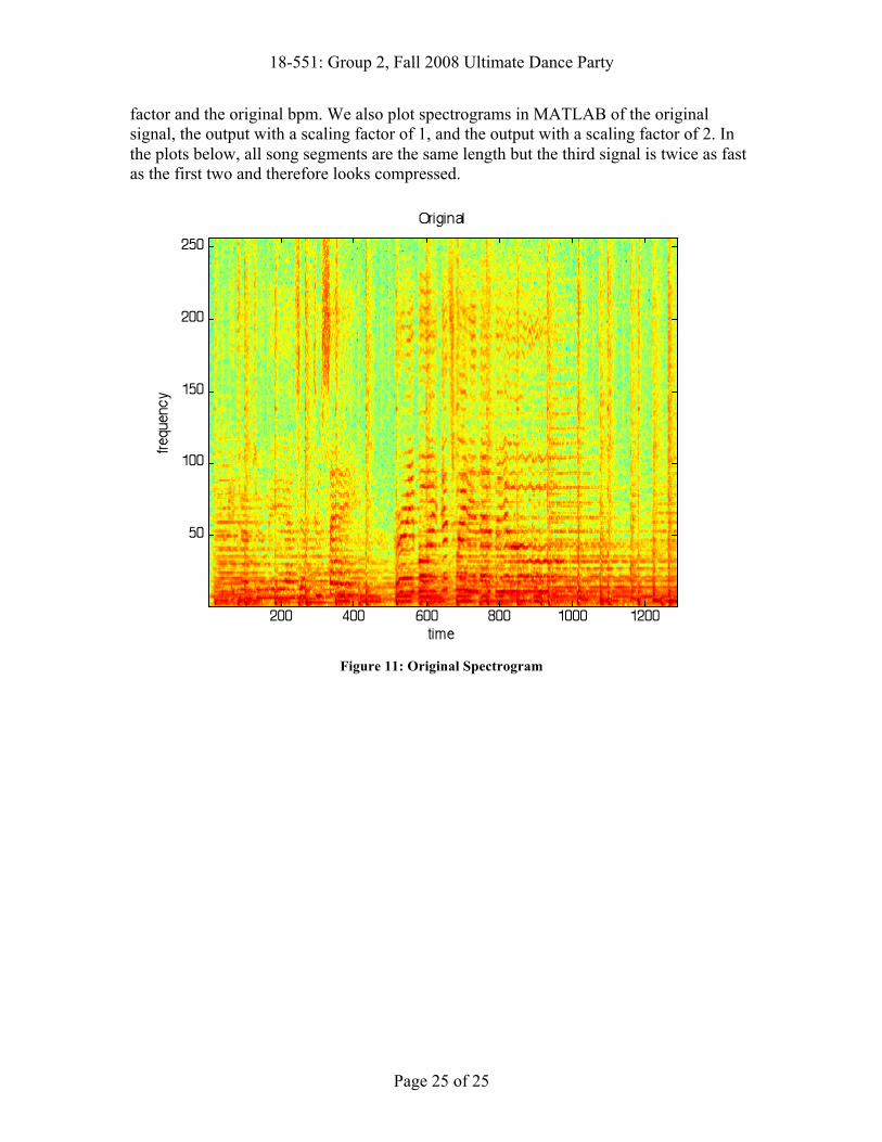
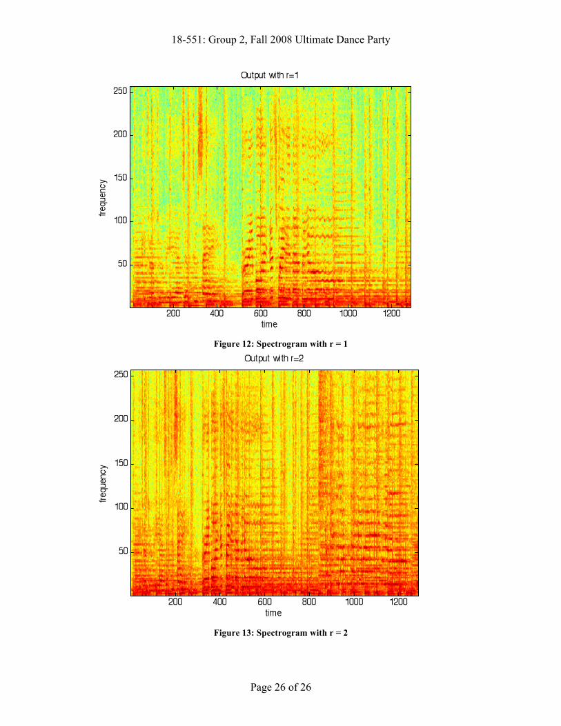
factor and the original bpm. We also plot spectrograms in MATLAB of the original signal, the output with a scaling factor of 1, and the output with a scaling factor of 2. In the plots below, all song segments are the same length but the third signal is twice as fast as the first two and therefore looks compressed.

Figure 11: Original Spectrogram


of 26

Figure 12: Spectrogram with r = 1

Figure 13: Spectrogram with r = 2


of 27

5.4 GUI Since a major part of the Demo would involve the user interaction with the GUI, copious amounts of effort was poured into the development of a Graphical User Interface that would be simple yet effective. Also, since beat detection was done on the PC and was already implemented in MATLAB, we decided to use the MATLAB GUI editor (guide). In order to transfer a song from MATLAB to the DSK, MATLAB’s MEX library was invoked so that MATLAB would be able to pass data back and forth from C code written on the PC. This involved researching the various intricacies that revolved around writing C code that can interface with MATLAB. This was not a trivial task. See the references section for a helpful website on using the MEX library in MATLAB. Much effort went into providing the user with a GUI that would execute tasks autonomously without manual help from the user (such as manually running separate C code). The main GUI screen is as follows.

Figure 14: Main GUI Screen

Result of beat detection

Acceptable scaling values


of 28

The GUI interfaces with MATLAB code on beat detection to compute the BPM of any wave file selected via a browse button. In addition, since beat detection can take anywhere from 5 to 10 seconds per song, a progress bar was added to the GUI to inform the user what the PC is doing. This progress bar not only computes percent done but also time left.

Figure 15: Progress Bar for Beat Detection

Dialog boxes were created and used for user confirmation. Since DSK processing can take anywhere from 10 to 30 seconds, it is necessary for the user to be absolute sure that they are ready to begin the phase vocoder progress on the DSK or risk losing their valuable time. In addition, entertainment was provided for the user to look at while the DSK is processing the song so that the user does not become overwhelmed with boredom. This entertainment came in the form of a popup playing a movie of a popular dancing banana within MATLAB.

Figure 16: Dialog box for sending song to DSK

Figure 17: Entertainment while phase vocoder is processing


of 29

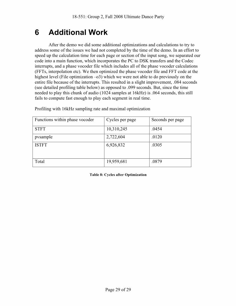
6 Additional Work

After the demo we did some additional optimizations and calculations to try to address some of the issues we had not completed by the time of the demo. In an effort to speed up the calculation time for each page or section of the input song, we separated our code into a main function, which incorporates the PC to DSK transfers and the Codec interrupts, and a phase vocoder file which includes all of the phase vocoder calculations (FFTs, interpolation etc). We then optimized the phase vocoder file and FFT code at the highest level (File optimization –o3) which we were not able to do previously on the entire file because of the interrupts. This resulted in a slight improvement, .084 seconds (see detailed profiling table below) as opposed to .099 seconds. But, since the time needed to play this chunk of audio (1024 samples at 16kHz) is .064 seconds, this still fails to compute fast enough to play each segment in real time. Profiling with 16kHz sampling rate and maximal optimization Functions within phase vocoder Cycles per page Seconds per page

STFT 10,310,245 .0454

pvsample 2,722,604 .0120

ISTFT 6,926,832 .0305

Total 19,959,681 .0879

Table 8: Cycles after Optimization


of 30

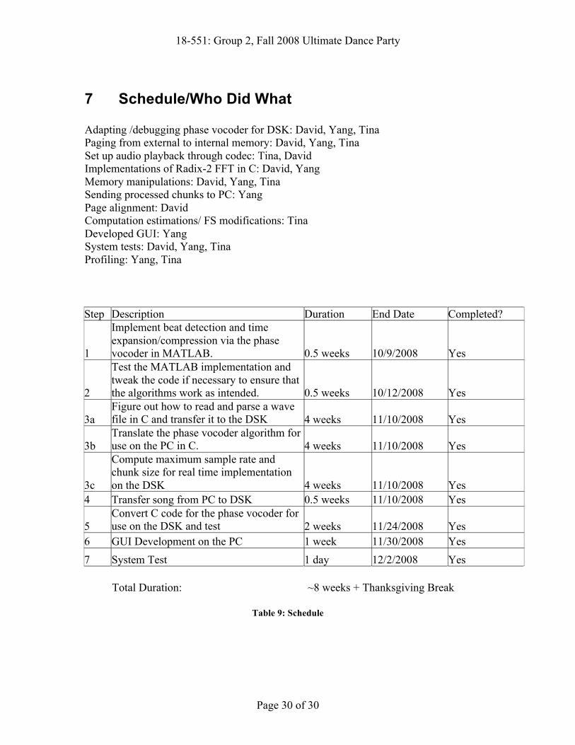
7 Schedule/Who Did What Adapting /debugging phase vocoder for DSK: David, Yang, Tina Paging from external to internal memory: David, Yang, Tina Set up audio playback through codec: Tina, David Implementations of Radix-2 FFT in C: David, Yang Memory manipulations: David, Yang, Tina Sending processed chunks to PC: Yang Page alignment: David Computation estimations/ FS modifications: Tina Developed GUI: Yang System tests: David, Yang, Tina Profiling: Yang, Tina Step Description Duration End Date Completed?

1

Implement beat detection and time expansion/compression via the phase vocoder in MATLAB. 0.5 weeks 10/9/2008 Yes

2

Test the MATLAB implementation and tweak the code if necessary to ensure that the algorithms work as intended. 0.5 weeks 10/12/2008 Yes

3a Figure out how to read and parse a wave file in C and transfer it to the DSK 4 weeks 11/10/2008 Yes

3b Translate the phase vocoder algorithm for use on the PC in C. 4 weeks 11/10/2008 Yes

3c

Compute maximum sample rate and chunk size for real time implementation on the DSK 4 weeks 11/10/2008 Yes

4 Transfer song from PC to DSK 0.5 weeks 11/10/2008 Yes

5 Convert C code for the phase vocoder for use on the DSK and test 2 weeks 11/24/2008 Yes

6 GUI Development on the PC 1 week 11/30/2008 Yes 7 System Test 1 day 12/2/2008 Yes Total Duration: ~8 weeks + Thanksgiving Break

Table 9: Schedule


of 31

8 Future Work

8.1 Using FastRTS A major improvement that could be implemented to speed up the processing on the DSK is the usage of FastRTS math functions instead of the regular rts6701 math functions. From figure 1 it can be seen that FastRTS can offer significant performance improvements, especially in areas where math functions are the major bottleneck. This is the case in our STFT and ISTFT functions.

8.1.1 Speed Estimates for STFT using FastRTS Time to compute magnitude and phase = (3*(time for powf) + (time for atan2f))*number of rows Total = (Time for FFT + Time to compute magnitude and phase) * number of columns

FFT Compute magnitude and phase

Number of Columns

Total Cycles

108,000 195,063 13 3,939,819

Table 10: STFT Estimate using FastRTS

8.1.2 ISTFT Estimate in Cycles Time to compute real and imaginary = (time for cosf + time for sinf) * number of rows Time to filter small numbers = (time for powf + time for fabs) * FFT Size Total = (Time to compute real and imaginary + time to filter small numbers + Time for IFFT) * number of columns IFFT Compute real

and imaginary Filter Number of

Columns Total Cycles

108,000 38,293 114,688 13 3,392,753

Table 11: ISTFT Estimate using FastRTS


of 32

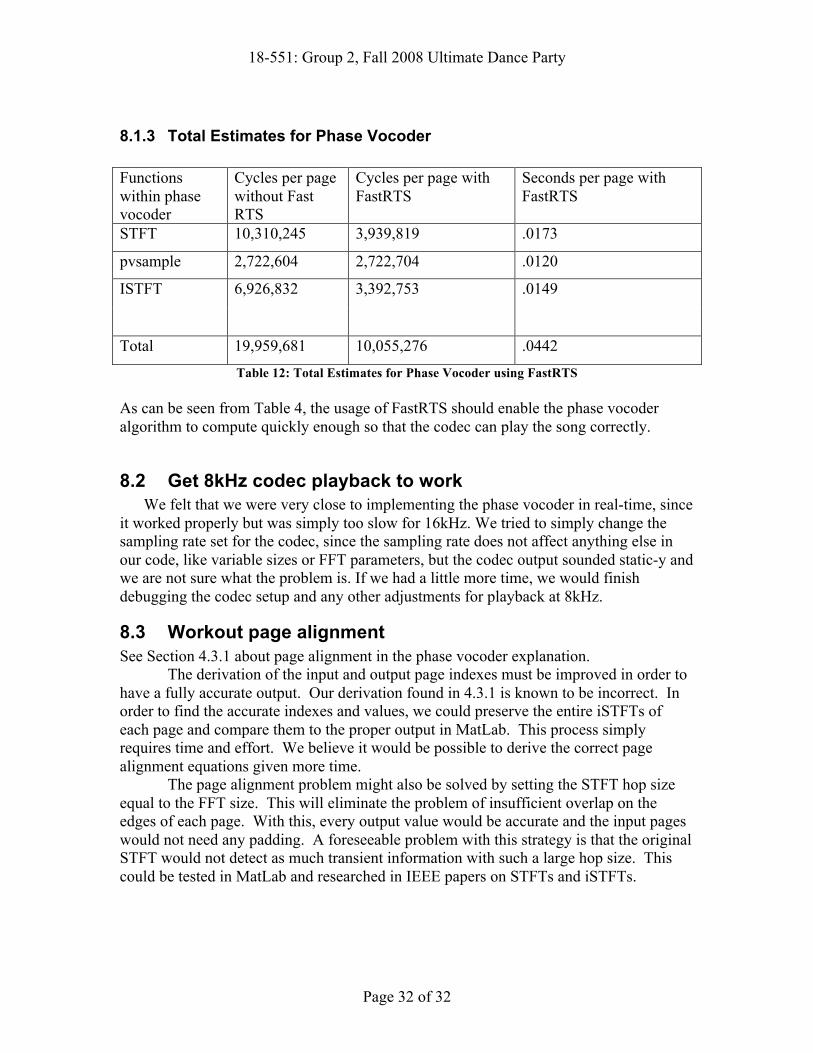
8.1.3 Total Estimates for Phase Vocoder Functions within phase vocoder

Cycles per page without Fast RTS

Cycles per page with FastRTS

Seconds per page with FastRTS

STFT 10,310,245 3,939,819 .0173

pvsample 2,722,604 2,722,704 .0120

ISTFT 6,926,832 3,392,753 .0149

Total 19,959,681 10,055,276 .0442 Table 12: Total Estimates for Phase Vocoder using FastRTS

As can be seen from Table 4, the usage of FastRTS should enable the phase vocoder algorithm to compute quickly enough so that the codec can play the song correctly.

8.2 Get 8kHz codec playback to work We felt that we were very close to implementing the phase vocoder in real-time, since

it worked properly but was simply too slow for 16kHz. We tried to simply change the sampling rate set for the codec, since the sampling rate does not affect anything else in our code, like variable sizes or FFT parameters, but the codec output sounded static-y and we are not sure what the problem is. If we had a little more time, we would finish debugging the codec setup and any other adjustments for playback at 8kHz.

8.3 Workout page alignment See Section 4.3.1 about page alignment in the phase vocoder explanation. The derivation of the input and output page indexes must be improved in order to have a fully accurate output. Our derivation found in 4.3.1 is known to be incorrect. In order to find the accurate indexes and values, we could preserve the entire iSTFTs of each page and compare them to the proper output in MatLab. This process simply requires time and effort. We believe it would be possible to derive the correct page alignment equations given more time. The page alignment problem might also be solved by setting the STFT hop size equal to the FFT size. This will eliminate the problem of insufficient overlap on the edges of each page. With this, every output value would be accurate and the input pages would not need any padding. A foreseeable problem with this strategy is that the original STFT would not detect as much transient information with such a large hop size. This could be tested in MatLab and researched in IEEE papers on STFTs and iSTFTs.


of 33

9 Additional References • MATLAB Code for phase vocoder

– A Phase Vocoder in MatLab Ellis Columbia University http://labrosa.ee.columbia.edu/MatLab/pvoc/

• MATLAB Code for beat detection algorithm – Beat This: A Beat Synchronization Project

Cheng, Nazer, Uppuluri, Verret Rice University http://www.owlnet.rice.edu/~elec301/Projects01/beat_sync/beatalgo.html

• FFT Code for phase vocoder testing on PC Side – From 18551 Homework 2

• ASM Code for FFT Routine on the DSK – Lab 2 (Texas Instruments) – DSPF_sp_cfftr4_dif -- Single Precision floating point Decimation in

Frequency radix-4 FFT with complex input • C Code for FFT Routine on the DSK

– Texas Instruments – DSPF_sp_fftSPxSP -- Single Precision floating point mixed radix

forwards FFT with complex input – DSPF_sp_ifftSPxSP -- Single Precision floating point mixed radix

inverse FFT with complex input • New Phase Vocoder Techniques for Pitch Shifting, Harmonizing and

Other Exotic Effects – Jean Laroche and Mark Dolson – http://www.ee.columbia.edu/~dpwe/papers/LaroD99-pvoc.pdf – Uses very similar phase vocoder algorithm, but for pitch detection/shifting

instead of time-scaling. Also suggests desirable parameters such as amount of overlap. However, Ellis documentation is more useful and ideal for our purposes

– Other IEEE resources were found to be overly convoluted and not aimed towards real-time time-scaling for music.

• Using the MEX Library in MATLAB – Provides examples of how to write C code so that MATLAB can call a C

file like it calls a function – Supports the passing of arguments/data from MATLAB to C and vice

versa. – https://people.scs.fsu.edu/~burkardt/m_src/MatLab_c/MatLab_c.html

ultimate dance party - carnegie mellon universityee551/projects/f08/g2_final...of course, the...

Documents