ultrasonic technique in determination of … · ultrasonic technique in determination of...
TRANSCRIPT
ULTRASONIC TECHNIQUE IN DETERMINATION OF GRID-GENERATED TURBULENT FLOW
CHARACTERISTICS
by
Tatiana A. Andreeva
A Dissertation
submitted to the Faculty of the
WORCESTER POLYTECHNIC INSTITUTE
in partial fulfillment of the requirements for the
Degree of Doctor of Philosophy
in
Mechanical Engineering
by
Tatiana A. Andreeva
October, 2003 Approved: Dr. William W. Durgin, Advisor Dr. Mikhail F. Dimentberg, Committee Member Dr. Zhikun Hou, Graduate Committee Representative Dr. David J. Olinger, Committee Member Dr. Suzanne L. Weekes, Committee Member

Abstract
The present study utilizes the ultrasonic travel-time technique to diagnose grid-
generated turbulence. The statistics of the travel-time variations of ultrasonic wave
propagation along a path are used to determine some metrics of the turbulence. The
motivation for this work stems from the observation of substantial delta-t variation in
ultrasonic measuring devices like flow meters and circulation meters. Typically,
averaging can be used to extract mean values from such time series. The corollary is that
the fluctuations contain information about the turbulence.
Experimental data were obtained for ultrasonic wave propagation downstream of a
heated grid in a wind tunnel. Such grid-generated turbulence is well characterized and
features a mean flow with superimposed velocity and temperature fluctuations. The
ultrasonic path could be perpendicular or oblique to the mean flow direction. Path
lengths were of the order of 0.3 m and the transducers were of 100 kHz working
frequency. The data acquisition and control system featured a very high-speed analog to
digital conversion card that enabled excellent resolution of ultrasonic signals.
Experimental data for the travel-time variance were validated using ray acoustic
theory along with the Kolmogorov “2/3” law. It is demonstrated that the ultrasonic
technique, together with theoretical models, provides a basis for turbulent flow
diagnostics. As a result, the structure constant appearing in the Kolmogorov “2/3” law is
determined based on the experimental data.
The effect of turbulence on acoustic waves, in terms of the travel time, was studied
for various mean velocities and for different angular orientations of the acoustic waves
i

with respect to the mean flow. Average travel time in the presence of turbulence was
shorter then in the undisturbed media. The effect of the time shift between the travel
times in turbulent and undisturbed media is associated with Fermat’s principle.
The travel time and log-amplitude variance of acoustic waves were investigated as
functions of travel distance and mean velocity over a range of Reynolds number varying
from 4000 to 20000. Experimental data are interpreted using classical ray acoustic
approach and the parabolic acoustic equation approach together with the perturbation
method. It was experimentally demonstrated that there is a strong dependence of the
travel time on the mean velocity even in the case where the propagation of acoustic
waves is perpendicular to the mean velocity. The effect of thermal fluctuations, which
result in fluctuations of sound speed, was studied for two temperatures of the grid: 59
(no grid heating) and 159 . A semi analytical acoustic propagation model that allows
determination of the spacial correlation functions of flow field is developed based on the
classical flow meter equation and statistics of the travel time of acoustic waves traveling
through the velocity and the thermal turbulence. The basic flow meter equation is
reconsidered in order to take into account sound speed fluctuations and turbulent
velocity. The resulting equation is written in terms of correlation functions of travel time,
sound speed fluctuation and turbulent velocity fluctuations. Experimentally measured
travel time statistics data with and without grid heating are approximated by Gaussian
function and used to solve the integral flow meter equation in terms of correlation
functions analytically.
Fo
Fo
ii
Acknowledgements I would like to express my deepest gratitude to my advisor, Professor William W.
Durgin. His knowledge and guidance inspired me to continue my education and try to
reach far beyond the level that I have now and had before. I would like to thank him for
his personal support, trust, and understanding throughout these years. Financial support
that he provided is deeply appreciated.
I would like to thank my entire committee Professor Zhikun Hou, Professor David J.
Olinger, Professor Suzanne L. Weekes, and especially Professor Mikhail F. Dimentberg,
who provided invaluable feedback during this work.
I would like to thank Professor Vladimir Palmov for his contribution to this work.
I would like to thank the following people for their assistance and support: Barbara
Furhman, Janice Dresser, Pam St. Louis, Gail Hayes, Nancy Hickman, Siamak Najafi,
Frank Weber.
I would like to express my admiration to Barbara Edilberti for her friendship and
moral support.
My thanks are extended to all my friends outside the school.
My special gratitude to my mother. Her love and belief in me lit the path for me
throughout my life.
And lastly, my very special thanks to my husband, Daniil, for his profound and
unconditional love. I would not have been able to complete this work without his support.
iii

Table of Contents
LIST OF FIGURES
LIST OF TABLES
NOMENCLATURE
CHAPTER 1. INTRODUCTION.................................................................................... 1
1.1 Theoretical, Computational and Experimental Issues in a Theory of Sound Propagation in a Moving Random Media............................................................... 4
1.1.1 Review of Theoretical Investigations ................................................................ 4
1.1.2 Review of Experimental Issues in Waves Propagation in Random Media........ 8
1.1.3 Review of Experimental Issues in Ultrasonic Technique ................................ 10
1.1.4 Review of Numerical Works in Modeling of Sound Propagation in Moving
Random Media ................................................................................................ 13
1.2 Objectives and Approach ........................................................................................ 14
CHAPTER 2. ISOTROPIC TURBULENCE............................................................... 16
2.1 Statistical Characteristics of the Medium................................................................ 16
2.1.1 Stationary Random Functions.......................................................................... 17
2.1.2 Random Functions with Stationary Increments ............................................... 19
2.1.3 Homogeneous and Isotropic Random Fields ................................................... 20
2.1.4 Locally Homogeneous and Isotropic Random Fields ...................................... 21
2.1.5 Frozen Turbulence Hypothesis ........................................................................ 22
2.2 Turbulence Spectral Models for Sound Propagation in Inhomogeneous Media .... 23
iv

2.2.1 Length Scales in Turbulent Flows ................................................................... 23
2.2.2 Isotropic Turbulence Spectrum Models........................................................... 25
2.3 Wind Tunnel Turbulence ........................................................................................ 29
2.3.1 Description of Ideal Grid Turbulence .............................................................. 29
2.3.2 The Decay of Flow Parameters Downstream of the Grid................................ 30
CHAPTER 3. SOUND PROPAGATION IN A MOVING RANDOM MEDIA ....... 32
3.1 The Aerodynamic Equations of a Compressible Gas.............................................. 33
3.2 The Acoustic Equations in the Absence of Wind ................................................... 37
3.3 Fundamental Acoustic Equations of the Moving Medium ..................................... 42
3.4 Ray Acoustics Approach......................................................................................... 44
3.4.1 Eikonal Equation.............................................................................................. 47
3.4.2 Fermat’s Principle ............................................................................................ 49
3.5 Turbulence of the Atmosphere, Travel-time Fluctuations, Kolmogorov’s “2/3” law......................................................................................................................... 50
3.6 Travel-time Statistics of Acoustic Waves as an Experimental Tool for Diagnostic of Turbulent Medium.......................................................................... 56
3.7 Parabolic Equation Approximation......................................................................... 59
CHAPTER 4. EXPERIMENTAL APPARATUS ........................................................ 64
4.1 Wind Tunnel............................................................................................................ 64
4.1.1 Boundary Layer ............................................................................................... 65
4.2 The Grid .................................................................................................................. 66
4.3 Description of the Ultrasonic System...................................................................... 67
4.3.1 Transit Time Flowmeters ................................................................................. 67
4.3.2 Data Acquisition and Analysis System............................................................ 69
v
CHAPTER 5. EXPERIMENTAL RESULTS AND DISCUSSION........................... 76
5.1 Application of Travel-time Ultrasonic Techniques for Data Acquisition............... 76
5.2 Ray Acoustics Approach......................................................................................... 79
5.2.1 Travel time fluctuations as a function of a separation distance . ................. 79 L
5.2.2 Transit Time Fluctuations as a Function of the Mean Velocity U . ................ 82
5.3 Parabolic Equation and Perturbation Method (Rytov’s Method)............................ 84
5.3.1 Travel Time Fluctuations as a Function of Mean Velocity and Travel
Distance. .......................................................................................................... 85
5.3.2 Travel-time and Log-Amplitude Variances ..................................................... 88
5.4 Methodology for Determination of Statistical Characteristics of Grid Generated Turbulence ............................................................................................................ 90
5.4.1 Methodology for Determination of Correlation Functions of Velocity and
Acoustic Waves Fluctuations .......................................................................... 90
5.4.2 Spectrum of Grid-Generated Turbulent Flow.................................................. 97
CHAPTER 6. SUMMARY, CONCLUSIONS, RECOMMENDATIONS .............. 102
6.1 Summary and Conclusions.................................................................................... 102
6.2 Recommendations ................................................................................................. 107
BIBLIOGRAPHY…………..……………………..………………………..…………109
APPENDIX A………………..…………………………………………..…………….117
APPENDIX B…..……………..……………………………………………………….120
vi
List of Figures
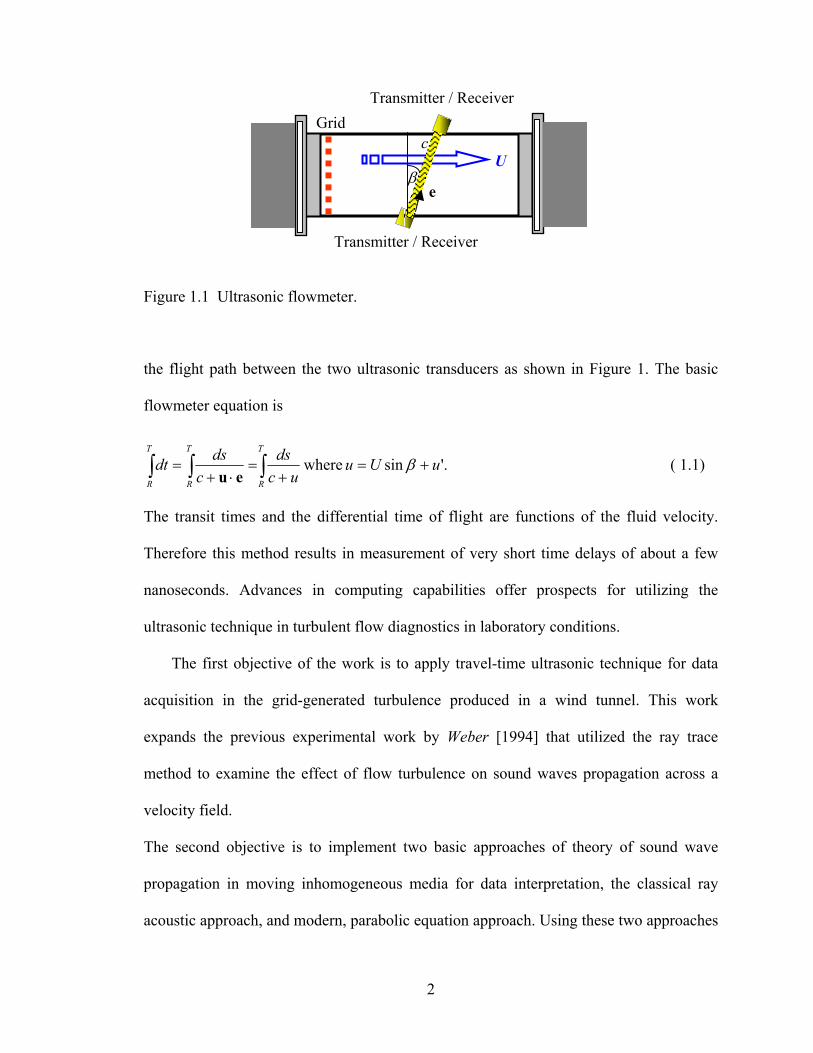
Figure 1.1 Ultrasonic flowmeter. ....................................................................................... 2
Figure 2.1 Example of realizations of random function u(t). .......................................... 17
Figure 2.2 Spectral view of three subranges of turbulence and corresponding length scales. .................................................................................................................... 25
Figure 2.3 Structure function with three limit approximations........................................ 26
Figure 2.4. Comparison of three 1-D primary turbulence spectra )(kF
const
and the corresponding length scales .................................................................................. 28
Figure 3.1. Kinematic relations in a geometrical theory of sound propagation............... 48
Figure 3.2. Surfaces of constant phase in an inhomogeneous medium. The rays are the curves perpendicular to the surfaces W = . ................................................. 49
Figure 3.3 Sketch of experimental setup......................................................................... 52
Figure 3.4. Sketch for the basic relations for the ultrasound measurement. .................... 53
Figure 3.5. Scheme of experimental setup....................................................................... 57
Figure 4.1. Sketch of the low turbulence, low speed research tunnel together with experimental setup. ............................................................................................... 65
Figure 4.2. Design characteristics of an ultrasonic transducer ........................................ 68
Figure 4.3. Transit-time ultrasonic flowmeter. ................................................................ 68
Figure 4.4. DAQ System Components ............................................................................ 70
Figure 4.5. Relationship between LabVIEW, Driver Software, and Measurement Hardware............................................................................................................... 71
Figure 4.6. Four-pulse burst of square shape waves........................................................ 72
Figure 4.7. Typical data representation obtained from CompuScope 82G DAQ, transferred to the PC and processed in Excel. Signals e1 and 2e are received and transmitted signals respectively. .................................................................... 73
vii

Figure 4.8. Magnification of received signal 1e e
5.3
and transmitted signal 2 , obtained from the digital data acquisition system CompuScope 82, shown in Figure 4.6.. 74
Figure 4.9. Block diagram of analog and digital processing. ........................................... 75
Figure 5.1. Sketch of wind-tunnel test section.................................................................. 79
Figure 5.2. Average travel time versus a path length, =U . ...................................... 81
Figure 5.3. Standard deviation of the travel time versus the travel distance, U 5.3= . ... 81
Figure 5.4. Correlation function 12K t of two waves. Maximum value of the correlation function corresponds to the travel time . .......................................... 82
( )t
0 m,33.0 == βL
0 m,33.0 == βL
L
o
Figure 5.5. Averaged travel time as a function of the mean velocity, . ................................................................................................. 83
Figure 5.6. Standard deviation of the travel time versus mean velocity, . ................................................................................................. 83
Figure 5.7. Variation of the structure constant C versus mean velocity. ......................... 84
Figure 5.8. Diagrams of the experimental setup that serves to investigate the average .. 85
Figure 5.9. Experimental data for mean travel time as a function of mean velocity for upstream and downstream propagation plotted along with theoretical estimates for the travel times in undisturbed medium. ......................................................... 86
Figure 5.10. Diagram of he experimental setup that serves to study the influence of the travel distance, .................................................................................................. 87
Figure 5.11. Experimental data for the travel time variance versus normalized travel distance. Rytov solution and theoretical model by Iooss et al. 2000 are plotted for comparison. ..................................................................................................... 88
Figure 5.12. Experimental data for the log-amplitude variance as a function of travel distance. Rytov solution for Kolmogorov spectra, Gaussian spectra and Frauhofer diffraction are plotted for comparison.................................................. 89
Figure 5.13. Correlation function of travel time obtained from experimental data collected at temperature of along with Gaussian function providing the best fit. 93
Figure 5.14. Experimentally obtained correlation function of turbulent velocity. ........... 94
Figure 5.15. Correlation function of travel time obtained from experimental data collected at temperature of 159 F along with Gaussian function providing the best fit.................................................................................................................... 94
viii
Figure 5.16. Difference in travel time correlation functions corresponding to temperatures and 159 Fo . ..................................................................................... 95
Figure 5.17. Correlation function of sound speed fluctuations......................................... 96
Figure 5.18. 1-D energy spectra of turbulent velocity and sound speed fluctuations..... 101
Figure 5.19. Comparison of 1-D energy spectrum of turbulent velocity recovered from experimentally measured travel time statistics with 1-D energy spectrum measured by Yeh and van Atta [1973] ............................................................... 101
Figure 6.1 The CS_SCOPE. VI Front Panel................................................................... 117
Figure 6.2. Gage Oscilloscope Sequence 0..................................................................... 118
Figure 6.3. Gage Sample Oscilloscope. VI (demonstration mode). ............................... 119
List of Tables
Table 5.1. Geometrical parameters. ................................................................................. 80
Table 5.2. Basic Parameters of the Flow Conditions for Heated Grid Turbulence at x/M=30. (Comparison with Yeh and Van Atta, 1973). ......................................... 98
ix
Nomenclature
B(u) Probability density function
c Speed of sound
effC Effective structure parameter
2uC Structure function parameter
c cv p, Specific heats at constant volume and constant pressure
( )21 , ttD Structure function of a random process
D Rod diameter
e Internal energy
tE Specific energy
k Wave number
K Correlation function
L Travel distance
0L Integral length scale
εl Characteristic inhomogenuity size
l Current length scale
Gl Gaussian length scale
vl Von Karman scale
M Grid size
),( 21 ttM Joint moment
r Distance between the observation points
P Pressure tensor
x
ijp Components of stress tensor
Pr Prandtl number
q Heat addition per unit mass
R Gas constant
Re Reynolds number
s Distance along a beam
S Entropy
t Travel time
T Mean temperature
T Stress tensor
U −x component of mean velocity
)(tu −x component of velocity at a fixed instant of time
),( rxv Complex wave amplitude
fV Phase velocity of a wave
Kv Kolmogorov velocity scale
Vol Specific volume
w Enthalpy
W Eikonal
α Mean dissipation rate of turbulent kinetic energy
β Coefficient of thermal expansion of air
2χ Variance of the log-amplitude of a wave
ε Index of refraction of sound waves
x y z, , Components of Cartesian position vector
xi
2φ Variance of phase fluctuations of a wave
( )ωΦ Spectral density
effΦ 3-D spectral density of a random field or an effective function
Π Velocity potential
γ Ratio of specific heats c cp v
η Kolmogorov microscale
λ Wave length
Tλ Taylor microscale
µv Viscosity coefficient
ν Kinematic viscousity
( )zyx ,,ν Complex wave amplitude
κ Thermal diffusivity
Æ Thermal conductivity
ρ Density
ijτ Components of viscous stress tensor
kτ Kolmogorov time scale
2σ Variance
ω Frequency of the sound wave
Superscripts
' Turbulent fluctuations
Subscripts
0 Ambient, undisturbed state of the medium
xii

Chapter 1. Introduction
This research investigates the influence of heated and non-heated grid-generated
turbulent flow on acoustic wave propagation. An acoustic wave carries some structural
information of the turbulent medium as a result of interaction with the medium so thus it
is possible to use some statistical characteristics of the acoustic wave as a diagnostic tool
to obtain some statistical information about the medium. Our interest in studying the
acoustic waves moving in a turbulent media is predicated on the fact that this problem is
found in many practical problems of atmospheric and oceanic acoustics and
aeroacoustics. Among these problems are noise pollution near highways, airports and
factories; acoustic remote sensing and tomography of the atmosphere and ocean;
detection, ranging and recognition of helicopters, aeroplanes, rockets and explosive
sources; and the study of noise emitted by nozzles and exhaust pipes.
The motivation of this study is recognition of the fact that ultrasonic technology is
evolving rapidly and technical advances offering great potential for performing
experimental investigations of statistical characteristics of turbulence in laboratory
conditions with high precision and non-invasively. Measuring flow parameters in
turbulent medium non-invasively and rapidly by means of ultrasound dating back to
experiments performed by Schmidt in 1970; demonstrated that ultrasonic flowmeters
provide many potential advantages over traditional techniques. The transit-time method is
the most widely used technique for ultrasonic flow metering. The principle is based on
modification of the time of flight of the ultrasound by the fluid velocity along the line of
1
Transmitter / Receiver
c
eβ
U
Grid
Transmitter / Receiver
Figure 1.1 Ultrasonic flowmeter.
the flight path between the two ultrasonic transducers as shown in Figure 1. The basic
flowmeter equation is
'.sin where uUuuc
dsc
dsdtT
R
T
R
T
R
+=+
=⋅+
= ∫∫∫ βeu
( 1.1)
The transit times and the differential time of flight are functions of the fluid velocity.
Therefore this method results in measurement of very short time delays of about a few
nanoseconds. Advances in computing capabilities offer prospects for utilizing the
ultrasonic technique in turbulent flow diagnostics in laboratory conditions.
The first objective of the work is to apply travel-time ultrasonic technique for data
acquisition in the grid-generated turbulence produced in a wind tunnel. This work
expands the previous experimental work by Weber [1994] that utilized the ray trace
method to examine the effect of flow turbulence on sound waves propagation across a
velocity field.
The second objective is to implement two basic approaches of theory of sound wave
propagation in moving inhomogeneous media for data interpretation, the classical ray
acoustic approach, and modern, parabolic equation approach. Using these two approaches
2
for interpretation of experimental measurements of travel time and wave amplitude an
investigation of the effect of turbulence on ultrasound wave propagation was conducted.
The work also demonstrates that combination of ultrasonic technique with one of the
theoretical models can be used to perform flow diagnostics.
Despite the advances in computing technology and consequently improvements in
measuring travel-time, ultrasonic flowmeter accuracy has not improved very much at all.
The explanation may lay in the effect of turbulence on ultrasound waves, namely velocity
and density fluctuations. To examine this possibility, the basic ultrasonic flowmeter
equation is reconsidered, where the effects of turbulent velocity and sound speed
fluctuations are included. The result is an integral equation in terms of correlation
functions of travel time, turbulent velocity and sound speed fluctuations. The third
objective is to develop an acoustic propagation model that allows determination of the
spatial correlation functions of travel time, turbulent velocity, sound speed fluctuations
and their spectra based on measured experimentally travel-time, thus identifying the
effect of sound speed fluctuations.
The intention to utilize ultrasonic methodology for turbulent flow diagnostics is also
motivated by the difficulty of obtaining laboratory measurements of time-of-flight
variance indicated by the dearth of data. Although a large number of atmospheric
measurements were made, they suffered from a lack of reliability and accuracy in
addition to poor characterization of the turbulence. The problem of travel-time
fluctuations is equivalent to the problem of finding the auto-correlation functions of these
fluctuations, which involves enormous amounts of experimental data and a large amount
of computational work. From the point of view of repeatability of experiments, it is much
3
more complicated and time-consuming to conduct outdoor experiments as compared to
those performed under convenient laboratory conditions. On the other hand, current
ultrasonic flow metering technology benefits from simple design and ease of operation
assuring high measurement precision.
1.1 Theoretical, Computational and Experimental Issues in a Theory of Sound
Propagation in a Moving Random Media
Our interest is concentrated on the effect of turbulence on sound wave propagation.
The random changes of velocity and temperature produced by turbulence are very rapid
and affect the sound propagation. This area of research lies on the boundary between
acoustics and aerodynamics. The present research is a result of experimental and
theoretical approaches. The literature review presents both classical and new results of
the theory of sound propagation in media with random inhomogeneities of sound speed,
density and medium velocity.
1.1.1 Review of Theoretical Investigations
The classical theory of wave propagation in turbulent media considers wave
propagation in isotropic or locally isotropic and homogeneous random media and based
on statistical representation of the turbulence [Chernov, 1960; Tatrskii, 1961, 1971;
Ishimaru, 1978]. The statistical moments of phase and log-amplitude fluctuations of a
sound wave propagating in the turbulent atmosphere have been calculated by Tatarskii
[1961] using the ray approximation and the Rytov method [Monin and Yaglom, 1981;
Brown and Hall, 1978]. Ray acoustics have been a standard approach for rigorous
consideration of sound wave parameters for outdoor experiments. The main advantages
4
of the ray theory of wave propagation are the clarity of its physics and relative simplicity.
The main results of geometrical acoustics were obtained before the mid-1940s and
summarized in the book by Blokhintzev [1953]. Nevertheless, until recently there was no
detailed treatment of geometrical acoustics in an inhomogeneous moving medium. The
main ideas are systematically reviewed in monograph by Ostashev [1997]. However, in
most cases, all scales of heterogeneities must be considered and mathematical conditions
for ray solutions are seldom met outdoors. Moreover, for example, in statistical
tomography in seismic media, all scales of heterogeneities are present so that scattering
occurs rapidly and geometrical optics fails [Samuelides, 1998; Iooss, 2000].
The modern theory of sound propagation in a moving random medium has been
developing intensively since mid-1980s. The governing system of linearized system of
equations of fluid dynamics, which allows description of the propagation of sound waves
in moving media, is rather complicated. Scientists have been trying to reduce it to a
single equation using various approximations and assumptions about a moving medium.
The most widely used single equation approaches in atmospheric acoustics are: Monin’s
equation [Tatarskii, 1961], Pierce’s equation [Pierce, 1990], parabolic equation [Rytov et
al., 1978]. The statistical characteristics of sound waves propagating in a moving random
medium with an arbitrary state equation have been calculated by the ray acoustics
method, Rytov and parabolic-equation methods. Efforts focusing on the stochastic
Helmholtz equation and its parabolic approximation are especially of interest.
The parabolic equation method is a very powerful method in the theory of wave
propagation. In certain cases it allows significant simplification of an analytical or
numerical solution of the problem. For describing acoustics in a moving medium, several
5

parabolic wave equations have been obtained [Godin, 1987; Nghiem-Phu and Tappert,
1985, Ostashev, 1987, Robertson et al., 1985]. In this approach the small perturbation
method is the most used solution to the parabolic approximation [Rytov et al., 1978;
Ostashev, 1997; Samueldis, 1998]. Clifford and Lataitis [1983] used the Rytov method to
calculate phase and log-amplitude fluctuations of the direct and ground-reflected waves
due to refractive index fluctuations. They followed Tatarskii, who considered the case,
when refractive index fluctuations are caused by temperature fluctuations. Furthermore,
Clifford and Lataitis calculated mean squared sound pressure by an energy conserving
approach. They presented a formula for mean squared sound pressure for a Gaussian
correlation function of refractive index fluctuations. These results made a significant
contribution to the development of atmospheric acoustics. Since the publication by
Clifford and Lataitis paper, the theory of atmospheric acoustics has been developed
significantly.
The effect of wind velocity and temperature fluctuations on the statistical moments
of a sound field was studied by numerous authors: Ostashev [1997, and references
therein], Ostashev and Wilson [1999]; Ostashev et al. [2001], Blanc-Benon et al. [1991],
Wilson [2000, and references therein]. Generalization of the theory by Clifford and
Lataitis was found in Ostashev and Goedecke [1998]; Ostashev et al. [2001]. The Rytov
approximation permits one to deal with log-amplitude and travel time fluctuations.
Lately, two effects of random heterogeneities have been investigated. First, the velocity
shift, which states, that the apparent velocity of the wave is greater than the average
sound velocity of the non-turbulent medium. This is in accordance with Fermat’s
principle, which states that the wave path minimizes the travel time of the wave [Landau
6
and Lifshitz, 1959]. This effect was discovered in the late 1980’s. The particular interest
to this effect lies in the area of surface seismic deterministic methods [Boyse, 1986, 1994;
Roth, 1993; Wielandt, 1987; Iooss and Galli, 2000]. Theoretical methods are based on
small perturbations in geometrical optics [Snieder and Aldridg, 1995 Boyse and Keller,
1994]. The results showed that if the magnitude of the heterogeneities is sufficiently
small, the relative velocity shift increases linearly with the propagation distance. In
seismology the determination of travel time is an important issue. Hence, the second
effect is the linear increase of the first-order travel-time variance with the propagation
distance [Chernov, 1960]. However, nonlinear effects appear at certain propagation
distances [Karweit et al., 1991; Iooss, 2000]. Overall, since the mid 1980s the rigorous
theory of line-of sight sound propagation through media with random inhomogeneities of
medium velocity, temperature has been developed; the statistical characteristics of the
sound wave have been calculated using the Born approximation, by ray, Rytov and
parabolic-equation methods, by the theory of multiple scattering and the diagram
technique [Ostashev, 1997]. Statistical characteristics are obtained for different models of
the random fields of velocity and temperature; homogeneous turbulence, homogeneous
and isotropic turbulence, turbulence with the Kolmogorov spectrum and Gaussian
correlation functions [Ostashev, 1997].
Further extension of our knowledge of sound propagation in the turbulent
atmosphere requires the validation of theory by experiments carried out outdoors and in
wind tunnels. Until recently, although a large number of atmospheric measurements were
made, they suffered a lack of reliability and accuracy in addition to poor characterization
of the turbulence. Laboratory experiments, despite there crucial importance, are
7
extremely rare. The objective in this dissertation is to demonstrate that ultrasonic
technology can be effectively utilized for data acquisition and flow diagnostics in
laboratory conditions.
1.1.2 Review of Experimental Issues in Waves Propagation in Random Media
We consider a locally isotropic, passive temperature field coupled with a locally
isotropic velocity field, which is realized by introducing a heated grid in a uniform flow
[Yeh and Van Atta, 1973 and references therein]. If temperature fluctuations are
sufficiently small then density is effectively constant and buoyancy forces are negligible.
Statistical turbulence data from hot and cold wire anemometry that describe the
temperature and velocity field downstream of a heated grid in a low speed wind tunnel
are typically given in the form of downstream decay of turbulence intensities, energy
spectra, autocorrelations, spatially separated cross correlations, phase, coherence
[Comte-Bellot and Corrsin, 1971; Yeh and Van Atta, 1973; Sepri, 1976; Warhaft and
Lumley, 1978; Sreenivasan et al, 1980; Van Atta, 1991; Nelkin, 1991; Sreenivasan and
Antonia, 1997; Warhaft (and references therein), 2000].
The influence of turbulence on sound wave propagation has been studied by a
number of authors, who conducted a variety of experiments and provided a wide range of
experimental and analytical results in this area for the last fifty years. The book by
Tatarskii [1971] and paper by Brawn and Hall [1978] present a detailed review of the
research into sound propagation in turbulent atmosphere prior to the mid 1970. Recently
outdoor sound propagation in a turbulent medium has received serious attention.
Measurements of the intensity fluctuations in the atmosphere or ocean have been
obtained by Daigle et al. [1978, 1983, 1986]; Ewart et al. [1986]. Experimental
8
measurements of sound propagation through the atmosphere with particular emphasis on
amplitude and phase fluctuations due to atmospheric turbulence were performed by Bass
et al, [1991 and references therein]. Particular interest to large-scale turbulence was paid
by Chessel, [1976]; Roth [1983], Wilken, [1986]. Noble et al.[1992] provided
experimental evidences that large eddies cause phase fluctuations over a broad range of
frequencies. The acoustic propagation model that incorporates the current state of
understanding of a large-scale atmospheric turbulence structure was developed by Wilson
and Thompson [1994, references therein].
It has been emphasized that sound propagation is sensitive to random variations in
the effective refractive index, which is a function of temperature and medium velocity
fluctuations. Di Iorio and Farmer [1996] showed that the velocity fluctuations can be
dominant source of acoustic scattering and in their 1998 paper they showed that the
random variations in temperature also contribute to the total scattered signal. Although a
large number of atmospheric measurements were made, the uncertainties with regard to
relevant environmental parameters, namely velocity and temperature variations, make it
difficult to assess their individual influence on acoustic wave propagation. Moreover,
outdoor experiments suffered a lack of reliability and accuracy in addition to poor
characterization of the turbulence. The problem of phase fluctuations is equivalent to the
problem of finding the auto-correlation functions of these fluctuations, which involves
enormous amounts of experimental data and a large amount of computational work. From
the repeatability of experiments point of view, it is much more complicated and time-
consuming to conduct outdoor experiments compared to those performed under
convenient laboratory conditions. The challenge in conducting laboratory experiment is
9
first the fact that there is a dearth of reliable data collected in well-controlled
experimental conditions. Secondly, to demonstrate that rapidly evolving computational
technology and ultrasonic technique provide great potential for conducting acoustic
experiments in laboratory conditions that will lead to further extension of knowledge of
sound propagation in the turbulent atmosphere. The propagation of sound waves through
turbulent velocity fields has been previously investigated under laboratory conditions. Ho
and Kovasznay [1974] made such measurements across an air jet over an extremely short
propagation distance. Blanc Benon in his work in 1981 generated an approximately plane
acoustic wave with a pistonlike sound source and aimed it across jet-generated air flows.
In his later work, in 1993 together with Juve he presented experimental results for the
variance of the normalized intensity fluctuations and for the probability functions of
acoustic waves that propagate through thermal grid-generated turbulence. Experimental
data were obtained by varying both the frequency of the wave and the distance of
propagation. Although review of the literature reveals a substantial improvement in the
understanding of the sound propagation in the turbulent atmosphere, it is obvious that
experimental investigations performed in laboratory conditions are very rare.
1.1.3 Review of Experimental Issues in Ultrasonic Technique
The breakthrough in the problem of measuring flow parameters in a turbulent
medium using sound was made by Schmidt [1970, 1975], who discovered the possibility
of measuring flow parameters non-invasively and without perturbation by means of
ultrasound. His concern was in connection with his efforts to measure the circulation
associated with aerodynamic surfaces in a wind tunnel. Johari and Durgin [1998]
reported a number of applications that extended Schmidt’s initial work. Specifically, they
10
investigated unsteady flow about an airfoil, the trailing vortex from a delta wing, and
swirling free-surface flows.
During the past twenty five years ultrasonic technology has progressed very rapidly
and has been used to improve flow measurement accuracy, specifically the development
of the equipment capable of measuring the very small time differences associated with
changes in the ultrasound wave propagation time resulted in measuring devices with
accuracy of the order of 0.25%. An exhaustive review of recent works on theory,
techniques and applications of ultrasonic measurements is presented in the book by
Lynnworth [1989]. The study of the transmission and attenuation of the signal and noise
mechanism performed by Brassier et al. [2001] gives us a preferred choice of the
frequency at which ultrasonic transducers can be operated. In their work authors
presented an innovative prototype of the ultrasonic flow meter using optimal choice of
ultrasonic frequency, the design and the “echo process”. With improved technology we
are now able to measure volumetric flow rate and other flow parameters in pipes and
conduits reliably and accurately in laboratory scale apparatus.
The intention to utilize the principles of the ultrasonic flowmeter for turbulent flow
diagnostics is motivated first by its advantages over traditional methods. The principle
advantages include noninvasiveness, relatively simple operation/installation, fast
response, high date rate, maintenance of long term accuracy be maintained, low
production cost, unit-to –unit interchangeability. Secondly, our interest in the ultrasonic
technique is substantiated by its broad range of applications in many engineering and
scientific fields. Potential applications include, but not limited to marine aviation,
meteorological and industrial areas [Kits van Heyningen, 1987]. Other potential
11
applications are: high accuracy sensors as part of a wind shear warning system for
airports and for meteorological stations where maintenance and/or environmental
considerations make mechanical devices impractical [Lynnworth, 1989]. The National
Institute of Standards and Technology investigates ways to reduce the uncertainty and
improve the operational capability of flow calibration facilities. As understanding of
ultrasonic metering methods spreads through the flow metering community, these
methods may evolve into primary flow standards [Mattingly and Yeh, 2000]. There are
fundamental theoretical and computational issues related to the ultrasonic flowmeter
technique that must be understood and in some instances resolved. Industrial flowmeters
are designed for idealized flows: usually a mean velocity profile while turbulence
including velocity and temperature fluctuations is ignored. The presence of secondary
flows is known to cause significant metering inaccuracies, so it is clear that non-ideal
flows are of concern for accurate measurements. Yeh and his colleagues [Yeh and Espina,
2001; Yeh et al., 2001] have been working to develop an intelligent ultrasonic flow meter
that can identify swirl and cross flow characteristics and appropriately influence
volumetric flow rate calculations. The objective in this thesis is to account for some of
the aforementioned shortcomings by identifying the effect of turbulence on ultrasound
wave propagation including the effect of velocity and density fluctuations on travel time
of ultrasound wave. Our theoretical formulation of the basic ultrasonic flowmeter
includes sound speed fluctuations and velocity fluctuations terms.
12
1.1.4 Review of Numerical Works in Modeling of Sound Propagation in Moving
Random Media
Another rapidly developing approach, besides analytical and experimental, is the
numerical one. Calculation of sound propagation in atmosphere requires accurate
representation of turbulence spectrum. The complexity of the turbulence dynamics,
however, makes development of turbulence models for propagation calculations difficult.
Another practical difficulty is that turbulence modeling is associated with fully three-
dimensional spatial models of the turbulence. Structure along the direction of
propagation, as well as in the direction transverse, must be known. Some initial efforts in
multidimensional modeling of sound propagation in atmosphere have been made by
Kristensen et al. [1989]; Mann, [1994]; Peltier et al. [1996]; and Wilson [2000].
Recognition of the fact that large eddies, belonging to the energy-containing subrange,
play a significant role in acoustic scattering favors a Gaussian model over the
Kolmogorov one [Wilson and Thomson, 1994; Daigle et al., 1983; Jojnson et al.]. To
reconcile the Kolmogorov and Gaussian approaches, recent investigators used a von
Karman model for the turbulence spectrum (Wilson, 2000 and references therein). The
effect of turbulence on sound propagation through numerical simulations was
investigated in works by Karweit et al. [1991 and references therein], Ph. Blanc-Benon et
al. [1991,1995], Chevret [1996], Ioos et al [2000] analytically and numerically studied
the high frequency propagation of acoustic plane and spherical waves in random media.
Using ray acoustics and a perturbation approach they obtained the travel time variance at
the second order and demonstrated nonlinear behavior of travel time variance at large
propagation distances.
13
1.2 Objectives and Approach
The primary goal of this work is to determine turbulent flow characteristics from the
statistics of travel-time variations. The thesis includes theoretical modeling, experimental
measurements, and comparison (interpretation) of experimental data with known
theoretical, numerical and experimental data.
The theoretical modeling includes:
1. Development of an acoustical propagation model that allows determination of the
spatial correlation functions of travel time, turbulent velocity, sound speed
fluctuations and their spectra based on measured experimentally travel time.
2. Derivation of the flowmeter equation in terms of cross correlations of travel time,
turbulent velocity and sound speed fluctuations.
3. Application of the spectral analysis as a technique in obtaining integral solutions
for the correlation functions, which are of interest in themselves.
4. Development of a methodology for spectral analysis of isotropic homogeneous
turbulence.
The experimental investigation is primarily concerned with application of the travel time
ultrasonic technique for data acquisition in the grid-generated turbulence produced in a
wind tunnel. The ultrasonic technique implementation includes two different
experimental setups for both heated and non-heated grid-generated turbulence:
1. Travel time versus travel distance (downstream and upstream propagation of
ultrasound with respect to the mean velocity vector);
14

2. Travel time versus mean flow velocity (perpendicular propagation of ultrasound
waves with respect to the mean velocity vector).
The experimental data validation is based on well-known Kolmogorov law, derived
purely from the dimensional analysis. The interpretation of experimental data includes:
a) Ray acoustics approach for travel time interpretation and determination of
structure constant.
b) Stochastic Helmholtz equation, its parabolic approximation and the small
perturbation method as a solution to the parabolic approximation for log-
amplitude, travel-time variations interpretations.
c) Demonstration of Fermat’s principle.
d) A Gaussian turbulent spectra model for travel-time sound propagation.
The thesis is organized as follows. In Chapter 2 we review several topics from the
theory of random fields and turbulence theory. In Chapter 3 we present the fundamental
equations of the acoustics of a moving inhomogeneous medium with its further two
approximations: ray acoustics and stochastic Helmholtz equation along with Rytov
approach. In Chapter 3 we also review some physical and mathematical issues of the
theory of sound propagation in a random media. In Chapter 4 we present description of
experimental apparatus, generation of grid-generated turbulence using grids, ultrasonic
system, data acquisition and analysis system. Chapter 5 is devoted to the analysis of
experimental data, discussion of results and comparisons with theoretical and numerical
data. Conclusions and recommendations are presented in Chapter 6.
15

Chapter 2. Isotropic Turbulence
In this chapter we give a brief exposition of some topics from the theory of random
fields and turbulence theory, which are necessary in the following experimental and
theoretical analysis. We give special attention to the representation of isotropic
turbulence by means of correlation functions, spectral expansions based on the
wavelength scale. Review of isotropic, homogeneous turbulence characteristics is
followed by the outline of length scales in turbulent flows and corresponding turbulence
spectrum models. The second part of the chapter is devoted to the generation of
approximately isotropic homogeneous turbulence in a wind tunnel by means of a grid.
The relations for decay of velocity, temperature fluctuations, integral length scale
downstream of a grid are presented.
2.1 Statistical Characteristics of the Medium
In what follows we repeatedly need basic information about the statistical properties
of developed turbulent flow. In this chapter we present only those results of statistical
theory of random functions and fields, which are important for our purposes, and refer to
the original sources [Kolmogorov, 1941, 1963; Obukhov, 1941; Loitsyanskii, 1939,
Batchelor, 1953; Tatarskii, 1961, 1971; Monin and Yaglom, 1981; Landau and Lifshitz,
1959; Stratonovich, 1961] for more detailed information.
16
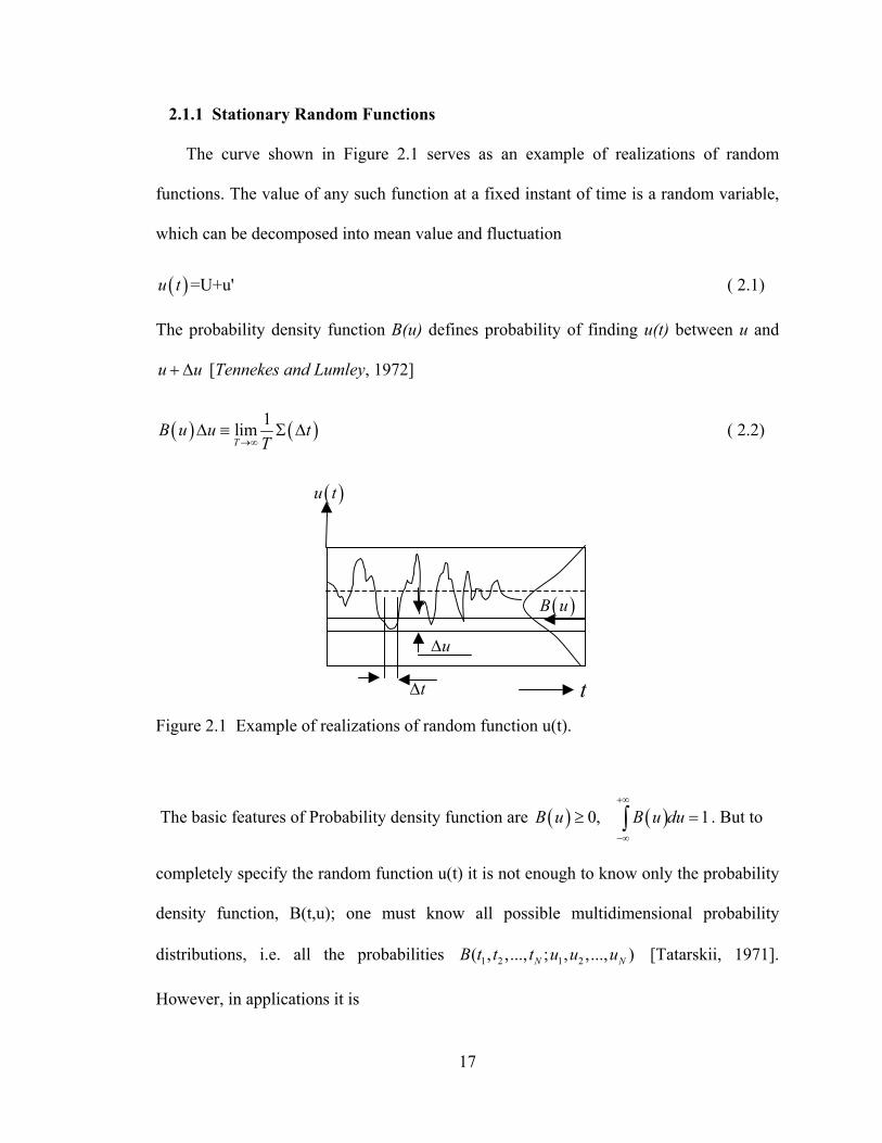
2.1.1 Stationary Random Functions
The curve shown in Figure 2.1 serves as an example of realizations of random
functions. The value of any such function at a fixed instant of time is a random variable,
which can be decomposed into mean value and fluctuation
( ) =U+u'u t ( 2.1)
The probability density function B(u) defines probability of finding u(t) between u and
[Tennekes and Lumley, 1972] u + ∆u
( ) (1limT
)B u u tT→∞
∆ ≡ Σ ∆ ( 2.2)
u∆
( )B u
tt∆
( )u t
Figure 2.1 Example of realizations of random function u(t).
The basic features of Probability density function are . But to ( ) ( )0, 1B u B u du+∞
−∞
≥ =∫
completely specify the random function u(t) it is not enough to know only the probability
density function, B(t,u); one must know all possible multidimensional probability
distributions, i.e. all the probabilities 1 2 1 2( , ,..., ; , ,..., )N NB t t t u u u [Tatarskii, 1971].
However, in applications it is
17

difficult to determine all the functions. It is customary used simpler characteristics of the
random field. They are called moments. The first moment is the mean value
( )U uB u du+∞
−∞
≡ ∫ . ( 2.3)
The second moment is a variance – mean square departure from the mean
( ) ( ) ( ) ( )22 2 2
1 1, ' = 'K t t u u t u t u B u duσ+∞
−∞
= ≡ − = ∫1 1 . ( 2.4)
The square root of variance is called standard deviation or rms amplitude. The joint
moment is
( ) ( ) ( ) ( )1 2 1 2 1 2 1 2 1 2, ,M t t u t u t u u B u u du du+∞ +∞
−∞ −∞
≡ = ∫ ∫ . ( 2.5).
The most important characteristic of a random function is its correlation function
[Tatarskii, 1961]
( ) ( ) ( ) ( )( ) ( )( ) ( ) ( )
1 2 1 2 1 1 2 2 1 2 1 2
1 2 1 2
, ' ' ,
,
K t t u t u t u u u u B u u du du
M t t u t u t
+∞ +∞
−∞ −∞
≡ = − −
= −
∫ ∫ =
2
. ( 2.6)
A random function u(t) is called stationary if its mean value does not depend on the time
and if its correlation function depends only on a difference [Tatarskii,
1961], i.e.
1 2( , )K t t 1t t−
( 2.7). 1 2 1 2( , ) ( )u uK t t K t t= −
For stationary random functions u(t) there exist expansions in Fourier integrals, namely a
stationary random function can be represented in the form of a stochastic Fourier-Stieltjes
18
integral with random complex amplitudes ( )ϕ ω , where ω is the frequency of the wave
[Tatarskii, 1961]
( ) i tu t e dωϕ ω+∞
−∞
= ∫ . ( 2.8)
Using the inverse Fourier transform, the function ( )ϕ ω can be expressed as follows:
1( ) ( )2
i tu t e dtωϕ ωπ
+∞−
−∞
= ∫ . ( 2.9)
The spectral density of the stationary random function u(t) by definition is [Rytov et al.,
1978] is
( ) ( ) ( )12
i tu uK t e dtωω
π
+∞−
−∞
Φ = ∫ . ( 2.10)
In its turn, a correlation function can be written as ( )uK t
( ) ( ) i tu uK t e dωω ω
+∞
−∞
= Φ∫ . ( 2.11)
Hence, and are Fourier transforms of each other. ( )uK t ( )u tΦ
2.1.2 Random Functions with Stationary Increments
In order to describe random functions that are more general then stationary random
functions, in turbulence theory a so-called structure function can be used instead of
correlation function [Kolmogorov, 1941; Obukhov, 1941]. The basic idea consists of the
following. In the case when u(t) represents a non-stationary random function, the
difference ( ) ( ) ( )uf t u t u tτ= + − can be considered instead of the random function u(t).
The advantage of this technique is in the fact that for values of τ , which are not too
19
large, slow changes in the function u(t) do not affect the value of this difference, and it
can be a stationary random function at least approximately. In the case where f(t) is a
stationary random function, the function u(t) is called a random function with stationary
increments. The function of arguments t where t and take the values 1 2, t 1 2t
1 1 2 2, , ,t t t tτ τ+
( )
+ is called the structure function of a random process and has the
following form
1 2, =uD t t u
1 2( , )uK u= r r
1 2( , ) (u uK Kr r
( )( )3
12
uπ
Φ =k
)uK r
( ( )
( ) ( ) 22t u t− 1 . ( 2.12)
2.1.3 Homogeneous and Isotropic Random Fields
For a random field u(r) (random function of three variables) a correlation function
can be defined as [Tatarskii, 1961]
1 1 2 2( ) ( ) ( ) ( )u u u− − r r r r . ( 2.13)
In the case of random fields the concept of stationarity generalizes to the concept of
homogeneity. A random field is called homogeneous if its mean value is a constant and if
its correlation function satisfies the relation
1 0 2 0, )= + +r r r r . ( 2.14)
Hence, the correlation function of a homogeneous random field depends only on 1 2−r . r
The spectral density function in a case of homogeneous random field is
( ) 3iuK e dω
+∞−
−∞∫ rr . ( 2.15) r
For even correlation functions ( ) (uK − =r , in particular, for correlation functions of
a real or isotropic field, spectral density is also even, )u uΦ − = Φr r . In this case, the
20
correlation function and spectral density can be expressed through cosine Fourier
transform:
( )( ) ( )3
1( ) cos2
u K dπ
+∞
−∞
Φ = ⋅∫ ∫ ∫k k r u r r . ( 2.16)
A homogeneous random field is called isotropic if the correlation function
depends only on
( )uK r
r = r , i.e. only on the distance between the observation points. In order
to derive an expression for the spectral density function in isotropic random field in the
integral (2.16) the spherical coordinates can be introduced and the angular integration
carried out. As a result we obtain an expression
( )20
1( ) sin( )2u uk rK r k
kπ
∞
∫ r drΦ = . ( 2.17)
2.1.4 Locally Homogeneous and Isotropic Random Fields
A very rough approximation for the spatial structure of atmospheric turbulence may
be obtained by applying the method of structure functions [Kolmogorov, 1941, Tatarskii,
1961]. The advantage of this approximation is in the fact that the difference between the
values of the field u(r) at two points r r is mainly affected by inhomogeneities of the
field u with characteristic size less than distance
1 2,
1 2−r r . If the distance is not too large,
the largest inhomogeneities have no effect on ( ) ( )u r1u −r 2 , and therefore the structure
function depends only on the difference 1 2−r r :
( ) ( ) ( ) (21 2 1 2 1 2, =uD u u D− = r r r r r r )u − . ( 2.18)
21
This local dependence is the basis of the concept of local homogeneity [Kolmogorov,
1941, Tatarskii, 1961]. A random field u(r) is said to be locally homogeneous in the
region G if the distribution functions of the random variable ( ) (1u u−r r )2 are invariant
with respect to shifts of the pair of points , as long as these points are located in the
region G. Thus, the mean value and the structure function (2.15) of locally homogeneous
random field depend only on
1 2,r r
21 −r [Kolmogorov, 1941, Tatarskii, 1961]. The
relationship between the spectral density function and the structure function can be
obtained as
r
( )( ) 2 1 cos ( )uD+∞
−∞
= − ⋅ Φ∫ ∫∫r k r u dk k . ( 2.19)
A locally homogeneous random field is said to be locally isotropic in the region G if
the distribution functions of the quantity ( ) ( )1 u−r r
1 2
2u are invariant with respect to
rotations and mirror reflections of the vector −r , as long as the points are located
in G [Kolmogorov, 1941, Tatarskii, 1961]. The structure function of a locally isotropic
random field depends only on
r 1 2,r r
1 2−r r :
( ) ( ) ( )[ ] ( )rDuuD u2
u =−+= 11 rrrr . ( 2.20)
In the case where the field is locally isotropic, equation (2.19) is
2sin( ) 8 1 ( )ukrD r k k dk
krπ
+∞
−∞
= − Φ ∫ u . ( 2.21)
2.1.5 Frozen Turbulence Hypothesis
Under some conditions, sound passes through the turbulence in a time that is short
compared to the timescales characteristic of the evolution of the turbulence. In such cases
22
the turbulence can be imagined as “frozen” during passage of the acoustic wave. If a real
field u(t,r) is stationary in time and homogeneous in space, it is described by means of
space-time correlation function
1( , ) ( , ) ( , )uK t u t t u t= +1r r + r r , ( 2.22)
assuming ( ) 0u =r . G. Tylor’s hypothesis [Tennekes and Lumley, 1972] states that the
entire spatial pattern of a random field is transported with the mean wind velocity U,
( , ') ( - ', )u uK t t K Ut+ =r r t . ( 2.23).
2.2 Turbulence Spectral Models for Sound Propagation in Inhomogeneous Media
In this subsection, isotropic models for the turbulence spectrum are presented on the
basis of the turbulence scales.
2.2.1 Length Scales in Turbulent Flows
No one model exists to accurately describe the entire turbulence spectrum in all
flows. It is important to know, which portion of the spectrum contributes significantly in
a given problem. There are three primary spectral subranges: the energy containing
subrange, the inertial subrange and the dissipation subrange, that are characterized by
their own length scales: Integral, Taylor and Kolmogorov respectively [Tennekes and
Lumley, 1972]. These subranges are schematically demonstrated in Figure 2.2. Whereas
the integral length scale is a characteristic length scale of the largest, most energetic,
and least dissipative motions, the Kolmogorov microscale
0L
η is the characteristic of the
23
smallest, most dissipative, and least energetic motions. The integral length scale is
defined by
0 20
1 ( )uL K rσ
∞
= ∫ dr . ( 2.24)
where uKu ,'22 =σ are the variance and autocorrelation of a velocity component (or
temperature), and r is the spatial displacement. By definition, the Kolmogorov microscale
is
( )1/ 43 /η ν ε= , ( 2.25)
where ε is a mean dissipation rate of turbulent kinetic energy. For velocity fluctuations,
for example, 21.5 /u d u dtε = − . In atmospheric turbulence, η is of order 1 to 10 mm,
many orders of magnitude smaller than . The inertial subrange consists of turbulent
motions having scales between
0L
L 0 and L η . The Taylor microscale Tλ falls within the
inertial subrange and is given in the isotropic turbulence by [Tennekes and Lumley, 1972]
22 15 u
Tσλ νε
= . ( 2.26)
The dissipation subrange can generally be ignored [Wilson et al, 1999] for the prediction
of acoustic propagation. For most frequencies the motions in the dissipation subrange are
very small compared to the acoustical wavelength and hence unimportant. Therefore, the
energy-containing and inertial subranges of atmospheric turbulence play the primary role.
It was demonstrated [Lawrence and Strohbehn, 1970; Wilson and Thompson, 1994] that
large scale energetic motions are responsible for phase fluctuations, while smaller scale
motions derive the amplitude fluctuations. However, the interplay between the
24
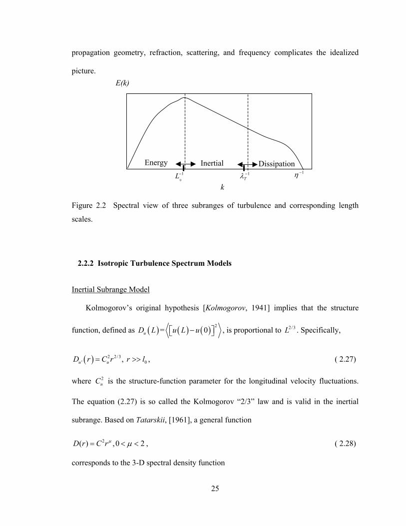
propagation geometry, refraction, scattering, and frequency complicates the idealized
picture.
k0
1L− 1Tλ − 1η −
E(k)
DissipationInertialEnergy
Figure 2.2 Spectral view of three subranges of turbulence and corresponding length
scales.
2.2.2 Isotropic Turbulence Spectrum Models
Inertial Subrange Model
Kolmogorov’s original hypothesis [Kolmogorov, 1941] implies that the structure
function, defined as ( ) ( ) ( ) 2=uD L u L u− 0 , is proportional to . Specifically, 2/3L
( ) 2 2/3' , u uD r C r r l= 0>>
<
, ( 2.27)
where is the structure-function parameter for the longitudinal velocity fluctuations.
The equation (2.27) is so called the Kolmogorov “2/3” law and is valid in the inertial
subrange. Based on Tatarskii, [1961], a general function
2uC
2( ) ,0 2D r C rµ µ= < , ( 2.28)
corresponds to the 3-D spectral density function
25

2 ( 32
( 2)( ) sin4 2
k C µµ πµπ
)k − +Γ + Φ =
. ( 2.29)
Consequently, the 1-D density for the inertial part of the spectrum is
2/3 5/3( )2u uk kα ε −Φ = , ( 2.30)
where α is a constant, whose value for atmosphere is approximately 0.52 [Högström,
1996].
For , structure function has a following form [Rytov et al., 1978] 0r << l
0<<
0>
( ) 4/32 2' 0 , u uD r C l r r l−= , ( 2.31)
Finally, at the structure function approaches the asymptotic value 0r L>>
( ) 2 2/3' 0 , u uD r C L r L= > , ( 2.32)
Figure 2.3 depicts a real structure function along with three approximations expressed by
equations (2.27, 2.31, 2.32) [Rytov et al., 1978].
( )D ∞
( )D r 2~D r 2/3~D r
0l 0Lr
Figure 2.3 Structure function with three limit approximations.
26
Gaussian Model
The starting point for the Gaussian model is the longitudinal velocity correlation
function
G
G
22
2expurKl
σ
= −
, ( 2.33)
where is the Gaussian length scale parameter. Fourier transformation yields the
spectrum
Gl
G
2 22G
G ( ) exp42
k llk σπ
Φ = −
. ( 2.34)
The Gaussian spectrum of inhomogeneities of the medium is very convenient for
analytical studies of wave propagation in random media. It allows accounting of the
effects of the largest inhomogeneities in a medium on the statistical moments of a sound
field [Rytov et al, 1978; Ostashev, 1997]. The Gaussian model is best suited for the
energy containing subrange. The Gaussian length scale parameter is the scale of the
largest inhomogeneities in a turbulent medium that affect the statistical moments of a
sound field [Ostashev, 1997]. In many practical cases l is of the order of , however,
can be less than . More advanced procedures for determination of the length scale
are described in Wilson [2000].
G 0L
Gl 0L
Von Karman Model
The von Karman model incorporates both the energy-containing and inertial
subranges [Ostashev, 1997]. The model is presented in many different, and not always
27
equivalent, forms in the literature. The correlation function for spatial separation parallel
to the direction of the velocity fluctuations, based on Wilson [2000] is
V
1/32
V
213
uLKl
σ = Γ
. ( 2.35)
The 1-D Fourier transform of the above correlation function is
( )( ) ( )V
2V
v 5/ 62 2
5 / 6( )
1/ 3 1
lkk l
σπΓ
Φ =Γ +
. ( 2.36)
A reasonable approach for determining the parameters in the von Karman model is to set
2σ to the actual variance of the field and then choose l to match the Kolmogorov model
in the inertial subrange. The von Karman model reduces, by design, to the inertial
subrange model. Qualitative comparison of three primary turbulence spectra is sketched
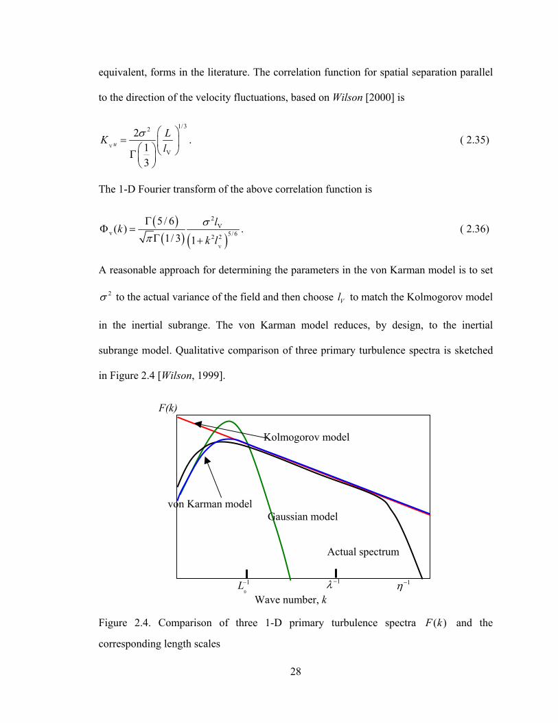
in Figure 2.4 [Wilson, 1999].
V
1λ −
0
1L− 1η−
Wave number, k
Kolmogorov model
von Karman model
Actual spectrum
Gaussian model
F(k)
Figure 2.4. Comparison of three 1-D primary turbulence spectra and the
corresponding length scales
)(kF
28
2.3 Wind Tunnel Turbulence
The following section is devoted to the description of the turbulence that may be
generated experimentally by the insertion of a grid into a low speed wind tunnel. The
actual experimental procedure is described in Chapter 5, while the theoretical issues are
considered here. Homogeneous, isotropic turbulence is considered an idealization that, at
most, can be achieved approximately in laboratory experiments.
2.3.1 Description of Ideal Grid Turbulence
The traditional method of generating, approximately, isotropic turbulence is by means
of a grid: a rectangular array of bars placed at the entrance of the test section [Batchelor,
1953; Comte-Bellot and Corrsin, 1966]. In practice the flow in a wind tunnel is
constrained by walls forming a finite boundary to the fluid motion. Boundary layer
effects are almost negligible for measurements made near the centerline of the tunnel. We
consider a fluid flow of infinite extent in its three spatial directions and being unconfined
by any boundaries. In the plane 0x x= a uniform grid is inserted. The grid is
characterized by two parameters: mesh size M and rod diameter D. The grid is imagined
to be of infinite extent in the plane such that the origin for the x-axis would be
indiscernible. The mean flow velocity is normal to the grid and is constant in time and
space (except in the immediate neighborhood of the grid). Sufficiently downstream of the
grid, the statistics of turbulence shall be assumed to be independent of (t,y,z) the cellular
flow generated by the grid having been consumed by the overall turbulent field. The
turbulence thus produced is statistically stationary, homogeneous with respect to
translations in the planes normal to the x-axis, and it decays in the downstream direction
of the grid. The above model shall be called ideal grid turbulence. For the generation of
29

thermal turbulence, the grid should be considered as being uniformly heated. Although
the thermal turbulence generated by heating the grid may exhibit large fluctuations, the
heat addition is small, so that there is no transfer of energy from thermal turbulence to
mean temperature. The thermal turbulence thus behaves like a passive scalar convected
by the mean velocity and is dissipated by conduction to the ultimate state of uniform
mean temperature [Sepri, 1976, Mydlarskii and Warhaft, 1998]. Since our research work
is not focused on investigation of turbulence characteristics, and the statistics of isotropic
turbulence are well known, we do not intend to go any further into representation of
equations of turbulence and statistics of turbulent flow. We limit ourselves to the
definitions and references.
2.3.2 The Decay of Flow Parameters Downstream of the Grid.
The Decay of Velocity Fluctuations
The downstream decay of the mean-squared streamwise turbulent velocity behind the
unheated grid is a relation of the type (Sreenivasan et al, 1980; Comte-Bellot & Corrsin,
1966; Kistler et al., 1954; Mills et al., 1958; Yeh & Van Atta, 1973; Warhaft & Lumley,
1978 (a,b))
20
12
nxu xU M M
α−
= −
, ( 2.37)
where 1 00.04, / 3, 1.2x M nα = = = are constants chosen to give the maximum possible
straight line fit to the experimental data in logarithmic co-ordinates [Sreenivasan et al,
1980].
The Decay of Temperature Fluctuations
30

The downstream decay of 2'T behind the heated grid is described by the relation of the
type
( )41 ,124.0,' 0
2
2
.mMx
Mx
TT m
==
−=
∆
−
ββ , ( 2.38)
where ,mβ were chosen as a best fit for experimental data [Sreenivasan et al, 1980]
The downstream development of the integral length scale
The expression for downstream decay of the integral length scale is
4.0013.0
−
−=
Mx
Mx
ML . ( 2.39)
The constants are chosen based on the best fit to the experimental data obtained by
Sreenivasan et al, [1980], Kistler et al, [1954], Mills et al, [1958], Yeh & Van Atta,
[1973].
31

Chapter 3. Sound Propagation in a Moving Random
Media
In this chapter, we present a derivation of the equations describing the propagation of
acoustical waves in inhomogeneous moving media. The main equations were obtained in
the literature by the mid forties [Blokhintzev, 1953; Kolmogorov, 1941; Chernov, 1960;
Tatarskii, 1961, 1967, 1971] while some of them have been derived just recently [Rytov
et al, 1978; Ostashev, 1997; Wilson, 1999, 2000]. The propagation of a sound wave in an
inhomogeneous moving medium is completely described by the system of linearized
equations of fluid dynamics. Then, starting from the general system of equations using
several assumptions with defined ranges of applicability, two well known approximate
theories of wave propagation, namely ray acoustics and the Rytov method are developed.
The statistical moments of a sound fields are calculated using these two approaches,
mainly following the reviews of published works [Tatarskii, 1967, 1971; Rytov, 1978;
Ostashev, 1997]. The eikonal equation and Fermat’s principle [Blokhintzev, 1953;
Landau and Lifshitz, 1959; Wilson, 1992] are discussed in application to the stationary,
inhomogeneous moving medium. The theory of travel-time fluctuations of sound waves
due to turbulence in the atmosphere based on a law, established by Obukhov [1941] and
Kolmogorov [1941], known as “2/3” law, is developed and the physical and mathematical
issues related to basic flowmeter equation are addressed. In subchapter 3.6 the classical
flowmeter equation is reconsidered in a form that includes turbulent velocity and sound
32

speed fluctuations. The result is an integral equation in terms of correlation functions for
travel time, turbulent velocity and sound speed fluctuations. Hence, the effect of velocity
and temperature fluctuations on acoustic wave propagation will be investigated. The
effect of these two factors in application to the flowmeter equation as well as a new
formulation of the classical flowmeter equation that has not been studied previously in
the literature will be shown.
3.1 The Aerodynamic Equations of a Compressible Gas
Any medium, in which sound is propagated, whether it is a gas, a liquid, or a solid,
has an atomic structure. However, it has been shown [Leontovich, 1936; Blokhintzev,
1953] that for a gas, if 1/ cf τ<< (where f is the sound frequency and cτ is the mean time
between collisions) the gas can be regarded as a continuous medium, which is
characterized by certain constants. Such a method of analysis is used in the theory of
aerodynamics [Blokhintzev, 1953]. The aerodynamic equations of a compressible gas are
taken as a basis of the theoretical analysis of the problem of the acoustics of a moving
medium. The aerodynamic equations of a compressible gas are expressed in three
fundamental conservation laws.
Continuity Equation
Assuming that there are no chemical reactions, the continuity equation is
( ) 0=⋅∇+∂∂ Vρρ
t. (3.1)
Momentum Equation
The general form of the momentum equation of is:
33
( ) ( ) gtρ ρ∂
+ ∇ ⋅ = ∇ ⋅ +∂
V VV P F . (3.2)
The pressure tensor is:
{ } .3,2,1,, where, =+−== jippp ijijijij τδP , ( 3.3)
where
=≠
=jiji
ij if 1 if 0
δ .
The term pij is the ij th components of the stress tensor acting on the area perpendicular to
ej with the direction given by ei. The term τ ij is the ij th components of the viscous stress
tensor T in accordance with Stokes theory, expressed for Newtonian fluids as
.3,2,1,,,32
=
∂∂
−
∂
∂+
∂∂
= kjixV
xV
xV
ijk
k
i
j
j
iv δµT , ( 3.4)
where µ is a viscosity coefficient. v
Energy Equation
( ) ( ) ( ) ( )t tE E pt
ρ ρ∂+ ∇ ⋅ = −∇ ⋅ + ∇ ⋅ + ∇ ⋅
∂V V T V q . ( 3.5)
The total specific energy Et is obtained as a sum of the specific internal energy e and the
specific kinetic energy
E e Vt = +
2
2. ( 3.6)
The heat transfer by conduction per unit mass is given by Fourier’s Law as
Tæ∇−=q , ( 3.7)
34

where the thermal conductivity æ is given by κρ 0cæ = , and κ is thermal diffusivity and
is specific heat at constant pressure. To the three basic laws of hydrodynamics there
must be added a constitutive equation such as the equation of state of the gas, which
connects the pressure, the density and the temperature:
pc
( , )p Z Tρ= . ( 3.8)
From the first law of thermodynamics we have for the energy per unit mass
de TdS pdVol= − , ( 3.9)
where S is the entropy, and Vol is a specific volume (Vol 1/ ρ= ). Then
2
de dS dVol dS p dT p Tdt dt dt dt dt
ρρ
= − = + . ( 3.10)
On the other hand,
( ) 2
d pdt t dt
p dρ ρ ρ ρρ ρ
∂ ∇ ⋅= + ⋅∇ = − ∇ ⋅ ⇒ = −
∂VV V ρ . ( 3.11)
The effect produced by viscosity and heat conduction in general energy balance usually
appears as small corrections [Blokhintzev, 1953] thus the process of sound propagation in
air is considered adiabatic. Consequently, for adiabatic processes we have
2
pde p d dp pedt dt
ρρ ρ ρ
= ⇒ = ∫ − , ( 3.12)
The quantity 2
pde p d p dpw edt dt
ρρ ρ ρ
= ⇒ = + = ∫ is known as enthalpy. If the process is
non-adiabatic, then equation (3.10) must be used. Then we get from equations (3.5) and
(3.10)
35

( )1 1dSTdt ρ ρ
= ∇ ⋅ + ∇ ⋅q T V . ( 3.13)
If we neglect æ and µ , since the effect produced by them in the general energy balance
usually negligible, we have
0dS S Sdt t
∂= + ⋅∇ =
∂V , ( 3.14)
i.e., the motion of fluid is adiabatic. If the motion is also irrotational, ∇× then the
Bernouilli theorem holds. It is convenient to introduce the velocity potential by putting
, momentum and energy equation (3.5) leads to
0=V
Π−= gradV
( )ρp
t∇
−=
Π∇+
∂Π∂
−∇ 25.0 . ( 3.15)
Taking into consideration that p wρ
∇= ∇ , integration of equation (3.15) yields
( )25.0 Π∇−∂Π∂
== ∫ tpw
p ρ. ( 3.16)
If the compressibility of the fluid is also neglected, then0
pw constρ
= + , consequently,
( ) constt
p +Π∇−∂Π∂
= 200 2
ρρ , ( 3.17
and for stationary flow,
( )22
2020 V
constconstpρρ
−=Π∇−= . ( 3.18).
The fact that the entropy of an ideal fluid ( )0æ == µ undergoing motion remains a
constant, makes it expedient to replace the variables ( ),Tρ in the equation of state (3.8)
36
by variables ( ) . , Sρ
3.2 The Acoustic Equations in the Absence of Wind
An oscillatory motion with small amplitude in a compressible fluid is called a sound
wave. The vibrations of the medium can be represented as acoustic vibrations under the
following assumptions:
1. Vibrations are small, so that any changes of state of the gas in an arbitrary small
volume can be neglected.
2. Frequencies under consideration are in the audible range (classical acoustics), or near
it (ultrasonic).
Based on aforementioned assumptions the terms of the second order can be neglected.
The relative changes in the fluid density and pressure are assumed to be small, namely
aappp ρρρ +=+= 00 , , ( 3.19)
where is the excess pressure, ap 0ρ is the density at 0p p= , 0T T= and ( is a
small velocity). In a similar fashion, we have for the temperature, entropy and energy
aVV = aV
aaa eeeSSSTTT +=+=+= 000 ,, . ( 3.20)
We then get from equations (3.1, 3.2)
Continuity Equation
00 =⋅∇+∂
∂a
a
tVρ
ρ. ( 3.21)
Momentum Equation
0312
0 =⋅∇∇+∇+−∇=∂
∂aaa
a pt
VVV
µµρ . ( 3.22)
37
The closure relation for an ideal gas is p RTρ= , where R is the gas constant per unit
mass. In terms of this becomes ( , Sρ )
0
0
expv
0p S Spc
γγρ
ρ −
=
v
, ( 3.23)
where is the specific heat at constant volume and vc /pc cγ = is the ratio of the specific
heats. The condition that the linearized equations of motion (3.21, 3.22) should be
applicable to the propagation of sound waves is that the velocity of the fluid particles in
the wave should be small compared with the velocity of sound: V c<<
0
. This condition
can be obtained, for example, from the requirement that ρρ <<a .
Energy Equation
For small changes in the state, equation (3.23) leads to [Blokhintzev, 1953]
vaaa
vaa c
phhSc
cpp
p 020
0
0 ...;... =++=++= ρρρρ
γ . ( 3.24)
For , the only term left is the one, which represents the small change in pressure
for small adiabatic expansions or compressions. The quantity
0=aS
0
0
pc γρ
= is adiabatic
sound velocity. The second term represents the change in pressure produced by the influx
or outflow of heat. The entropy changes satisfy equation (3.14), which, neglecting
quantities of second order, may be written in the form
aa Tt
ST 2
00
æ∇=
∂∂
ρ. ( 3.25)
Temperature changes T can be expressed in terms of the changes in the density and
entropy. Consequently, from equation (3.9)
a
38
eTS ρ
∂ = ∂ . ( 3.26)
The energy of an ideal gas is given by
( ) ( ) ( vav cSppTce /exp
11 0
10
γ
γ
ργρ
ργ −=
−==
−
) . ( 3.27)
Since aS
eSe
∂
∂=
∂
∂, equation (3.26) can be written in the form
( ) ( ) ( ) ργργρ
γ
γ
vva
v cpcS
cp
T1
/exp1 0
10
−=
−=
−
, ( 3.28)
i.e. for small changes of density and entropy
( ) ...1 0
20
20
0 +−
+=ργ
ρρρ
v
a
v
aa c
pcp
T . ( 3.29)
Here the first term represents the change in temperature, which follows from the adiabatic
expansion or compression of gas, while the second represents the change in temperature
due to a change in the entropy Substituting in equation (3.25) leads to
( )vaa
a cSt
S
01
21
2 1,ρ
γκκρκκ
−=∇+∇=
∂∂
. ( 3.30)
Equations (3.21, 3.22, 3.30) together with the equation of state (3.24) govern the
propagation of sound in a medium at rest, taking viscosity and heat conduction into
account. In all instances, in which sound absorption is not a matter of concern the
viscosity and thermal conductivity of the air can be ignored. Putting ( )0æ == µ leads to
, i.e. adiabatic sound propagation, and the governing equations are 0=aS
00 =⋅∇+∂
∂a
a
tVρρ , ( 3.31)
39

aa p
t
V−∇=
∂
∂0ρ , ( 3.32)
aa cp ρ2= . ( 3.33)
These equations can be solved using the velocity potential. Setting
aaa
a tp Π−∇=
∂Π∂
= V ;0ρ ( 3.34)
satisfies the equation (3.31). Then from equations (3.32, 3.33) the wave equation for the
potential is obtained
012
2
22 =
∂Π∂
−Π∇tc
aa . ( 3.35)
The wave is called plane wave if all its quantities depend only on one coordinate, for
example x-coordinate. That is, the flow is homogeneous in the yz-plane. The wave
equation (3.35) becomes
012
2
22
2
=∂Π∂
−∂Π∂
tcxaa . ( 3.36)
The solution of the equation (3.36) has the following form
( ) ( ctxfctxfa ++−=Π 21 ) . ( 3.37)
The distribution of the other quantities aaa Vp ,, ρ in a plane wave is given by functions
having the same form. If 2 0f = then, for density ( )ctxfa −= 1ρ . Expression
(1 )f x ct− represents a traveling plane wave. Since only xa
x ∂V Π∂= is non-zero
component of fluid velocity in a sound wave, sound wave in a fluid are longitudinal. In
the case of monochromatic waves all quantities are periodic (harmonic) functions of the
time. For example, velocity potential has the following form
40
( ) ([ tizyxre aa )]ω−Π=Π exp,,0 , ( 3.38)
where ω is the frequency of the wave. The function 0φ satisfies the equation
( ) 0/ 022
0 =Π+∆Π aa cω , ( 3.39)
which is obtained by substitution of equation (3.38) into the wave equation. In the case of
a monochromatic traveling plane wave, propagating in a positive direction of x-axis is
considered, the potential is of the form
(([ cxtiArea /exp −−=Π ))]ω , ( 3.40)
where A is a constant called the complex amplitude. Writing this as iA ae α= with real
constants a and α
[ ]αωω +−=Π tcxaa /cos , ( 3.41)
where a is called amplitude of the wave, and the argument of the cosine is called the
phase. If n is a unit vector in the direction of propagation, then the vector
( ) ( )/ 2 /cω π λ= =k n n
))]
( 3.42)
is called the wave vector, and its magnitude k the wave number. In terms of this vector
equation (3.40) can be written as
(([ tiArea ω−⋅−=Π rkexp . ( 3.43)
Any wave can be represented as a sum of superimposed monochromatic waves with
various wave vectors and frequencies. The decomposition of a wave into monochromatic
waves is an expansion as a Fourier series or integral.
41
3.3 Fundamental Acoustic Equations of the Moving Medium
Acoustic phenomena become more complicated in the presence of airflow. In the
general case, strictly speaking, it is not possible to distinguish acoustic phenomena from
the non-linear processes, which take place in a moving medium. For example, a current
of pulsating velocity acts on a microphone placed in the flow as if it were sound of the
corresponding frequency (provided that the frequency of these pulsations is sufficiently
high) although the velocity of propagation of these pulsations is different from the
velocity of sound. The relation between the pressure of these pulsations and their velocity
is non-linear and fundamentally different from the relation between the pressure and
velocity of sound wave. In order to distinguish sound propagation in a medium from
acoustic phenomena arising in the same medium as a result of motion of the medium, the
motion is considered to be frozen, i.e. it is assumed that motions in the flow are
sufficiently slow that
1/ fτ >> ( 3.44),
where τ is the time for an appreciable change in the state of flow [Tatarskii, 1961].
Supposing sound is propagated in the medium, the state of which is described by the
variables , , ,V p Sρ . The original state of the medium is considered as steady state and
the sound is regarded as a small perturbation, so that all the variables under consideration
have small fluctuations: aaaa SVp ,,, ρ . In order to obtain the equations of the sound
wave, the following replacements are introduced [Blokhintzev, 1953]
aaaa SSSpppVVV +=+=+=+= ,,, 00 ρρρ ( 3.45)
42
Limiting ourselves to the linear approximations, the terms of higher order of the
relatively small quantities aaaa SVp ,,, ρ . In addition, the irreversible processes, which
take place in sound propagation, are neglected. This means that in linear equations for
aaaa SVp ,,, ρ the terms that are proportional to viscosity and thermal conductivity are
neglected. Under the listed assumptions the fundamental acoustic equations of the
moving medium are [Blokhintzev, 1953]
0=⋅∇+⋅∇+∇⋅+∇⋅+∂
∂ VVVV aaaaa
tρρρρρ , ( 3.46)
( ) ( ) ( ) ( )2ρρ
ρaa
aaaa pp
tV ∇
+∇
−=⋅∇+××∇+××∇+∂
∂VVVVVV , ( 3.47)
0=∇⋅+∇⋅+∂
∂SS
tS
aaa VV . ( 3.48)
The equations of state are
ρρρρ
∂
∂=
∂
∂=+=
ph
pchScp
s
aaa ;; 22 . ( 3.49)
The linear character of the system of equations (3.46-3.49) requires small disturbances to
remain small in time, i.e. initial state is stable. The choice of thermodynamic variables
, Sρ is extremely useful for general theoretical considerations. For final numerical
calculations, however, the variables ,Tρ are more convenient. The quantities
,S
S∇pρ
∂ ∂
in terms of the variables p and T can be found in the following way.
The closed system of the linearized equations of fluid dynamics (3.46-3.49) gives the
starting equations for describing sound propagation in a moving medium. The first two
equations of this system were used in the first papers on acoustics in a moving medium.
43
All equations of this system were derived and used for the study of sound propagation by
Blokhintzev. In the system of fundamental equations (3.46-3.49) there are five unknown
even if one variable is eliminated by means of equation (3.49). The system therefore is
exceedingly complicated. The fundamental difficulty lies in the fact that as soon as the
pressure in the medium appears as a function of two coordinates , Sρ or ,Tρ , then even
in a quiescent medium, where there are no vortices and no current at all, the right hand
side of equation (3.46) will still not be a total differential and therefore sound will be
rotational. Important simplifications are obtained in the case when the changes in
aaaa SVp ,,, ρ are small over one wavelength of the sound. This approach is called ray
acoustics [Kolmogorov, 1941].
3.4 Ray Acoustics Approach
The basic characteristics of sound propagation in the atmosphere are determined by
slow changes in the state of the medium, for example, wind force, temperature and
density of the air. Under these conditions it is expedient to make use of the methods of
ray acoustics. In the following, the basic equations of ray acoustics are introduced in the
form that Blochintzev derived them. Starting with the system of equations (3.46-3.49), it
is assumed that flow parameters undergo only small changes within a single wavelength.
In order to make use of this fact in an approximate theory of sound propagation, it is
assumed that
00000
00
00
/2/ ,);exp();exp();exp( );exp(
λπωωρρ
==−=ΦΦ=Φ=Φ=Φ=
ckWktiSSiippiVV
aaaa
aaaa
, ( 3.50).
44
where ω is a sound frequency, 0 0 0/ 2 /k c 0ω π λ= =
0k
is the wave number in the
undisturbed state of the medium, W is called the eikonal. The following assumptions are
made in order to derive the system of ray acoustic equations [Blokhintzev, 1953]. The
quantities are considered to be slow changing functions of the
coordinated and time. The value of is considered to be large, so that the phase
changes very rapidly. The solutions for fluctuations of ambient flow parameters
0000 ,,, aaaa SpV ρ
aS
0k W
aV ,aap ,, ρ will be sought in the form of a series of inverse powers of the large
parameter ik 0
...;''
'...;''
'
...;''
'...;''
'
0
000
0
000
0
000
0
000
++=++=
++=++=
ik
SSS
ik
ik
ppp
ik
VVV
aaa
aaa
aaa
aaa
ρρρ
( 3.51)
Substituting (3.50) in equations (3.46-3.49) leads to the following system
( ) ( ) ( )
−∇+
∇−⋅∇−×∇×+×∇×−
∂∂
−=
=
∇−
200
20
0000
1
10
00 ,
chSppp
tb
bp
Wqik
aaaaaa
a
aa
ρρ
ρ
VVVVVVV
V
( 3.52 )
( )
( )[ ] ( ) ( ) VVVV
V
V
⋅∇−−⋅∇−⋅∇−−⋅
−−
∇⋅−
∂
∂+
∂
∂−=
=
∇−−
00200002
002
0
2
0
22
2002020
11
1'1'1
,''
aaaaaa
aaaa
aaa
hSpc
hSpc
hSpct
S
ct
p
cb
bWSc
hqp
c
qik
ρρ
ρ
( 3.53)
45
( ) ( )
refraction ofindex ; where
,,
0
000
3300
−∇⋅−=
∇⋅−∇⋅−∂
∂−==
c
qWcq
SSt
SbbqSik aa
aa
V
VV. ( 3.54).
Substituting (3.51) into system of equations (3.52-3.54) and collecting coefficients for
like powers the following two system of equations for zero and first power of ik
were obtained
0ik 0
For : ( )00ik
0'
' 00 =
−∇
ρa
ap
WqV , ( 3.55)
( ) 0''' 0002 =⋅∇−− WhSpcq
aaa Vρ , ( 3.56)
0' 0 =aqS ( 3.57).
For : ( )10ik
'1
00
'''' b
pWq a
a =
−∇
ρV , ( 3.58)
( ) '20002 '''''' bWhSp
cq
aaa =⋅∇−− Vρ , ( 3.59)
'30'' bqS a = , ( 3.60)
Here are the values of b b obtained upon substitution in them zero
approximations for V from equations (3.55-3.57). Solution of the system
of ray acoustic equations (3.55-3.57) leads to the eikonal equation and consequently to
the flowmeter equation. From the system of ray acoustic equations (3.58-3.60) an
equation for determination of sound pressure can be obtained. We conclude this
'3
'2
'1 ,, bbb 1 2 3, ,b
0000 ,,, aaaa Sp ρ
46
subchapter with a list of assumptions that define the range of applicability of the ray
acoustic approach [Rytov et al, 1978]:
, where is a characteristic inhomogenuity sizel lε ελ>>
, where is a travel distance; is a first Frenel zonel L L Lε λ λ>>
3.4.1 Eikonal Equation
We are concerned with a derivation of eikonal and flowmeter equations. In the
following, the derivation obtained by Blokhintzev is reproduced. Solution of the equations
(3.55-3.57) leads to the equation that connects particle velocity with pressure
( )ρ
00
'' aa
pqW∇
=V . ( 3.61)
By simultaneous solution of equations (3.56, 3.57) the equation of surface of constant
phase (W ) is obtained const=
22
2
qWc
∇ = . ( 3.62)
For V it follows from equation (3.54) that 0=
2220
2 2
cqc c
ε= = , ( 3.63),
where ε is the index of refraction of sound waves. The expression known as the eikonal
equation is
2 2W ε∇ = . ( 3.64)
47
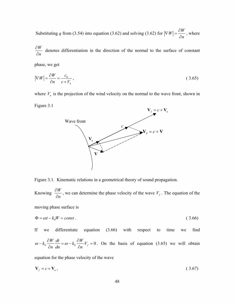
Substituting q from (3.54) into equation (3.62) and solving (3.62) for WWn
∂∇ =
∂, where
Wn
∂∂
denotes differentiation in the direction of the normal to the surface of constant
phase, we get
0
n
cWWn c V
∂∇ = =
∂ +, ( 3.65)
where V is the projection of the wind velocity on the normal to the wave front, shown in
Figure 3.1
n
Wave front
nV
c
f nc= +V V
V
S c= +V V
Figure 3.1. Kinematic relations in a geometrical theory of sound propagation.
Knowing Wn
∂∂
, we can determine the phase velocity of the wave V . The equation of the
moving phase surface is
f
0t k W constωΦ = − = . ( 3.66)
If we differentiate equation (3.66) with respect to time we find
0 0 0fW dt Wk kn dn n
ω ω∂ ∂− = −
∂ ∂V =
nV
. On the basis of equation (3.65) we will obtain
equation for the phase velocity of the wave
f c= +V , ( 3.67)
48

i.e. the phase velocity of the wave is equal to the local sound velocity plus the normal
component of the flow velocity. Kinematic relation is shown in Figure 3.1. Formula
(3.66) is one of the original assumptions in a geometrical theory of sound propagation.
3.4.2 Fermat’s Principle
Surfaces of constant phase are given by W const= , and therefore define the wave
fronts defined by equation (3.66) and shown in Figure 3.2 [Bergmann and Schaefer,
1999]. The direction of propagation is normal to the phase surfaces. It is the gradient
of the phase surfaces
n
gradWgradW
=n ( 3.68)
or, with equation (3.64)
gradWε =n . ( 3.69)
2W
1W
0W
En
n
E
Wave front
Figure 3.2. Surfaces of constant phase in an inhomogeneous medium. The rays are the
curves perpendicular to the surfaces W const= .
49
The beam propagation is in the direction of n . The curves, orthogonal to the phase
surfaces are called beams or rays, is the tangential vector to the beams. The difference
of two adjoining eikonals , whose distance along a beam is ds , is
n
dW
dW gradW ds= ⋅n , or with equation (3.69)
dW dsε= . ( 3.70)
The integral is the length of the optical path between a transmitter (T) and a receiver (R)
( ) ( )T
travel path= dsR
W T W Rε = −∫ . ( 3.71)
Fermat’s principle is a principle of extremum and says that the travel path between
transmitter and receiver always is an extremum [Bergmann and Schaefer, 1999]. The
length of the travel path, measured along a ray is always shorter then any other path
T T
R RrayS curveC
ds dsε ε≤∫ ∫ , ( 3.72)
where curve C is an arbitrary path. In terms of the travel time equation (3.72) has the
following form
( ) ( )2 1 2 1rayS curveCt t t t− < − . ( 3.73).
3.5 Turbulence of the Atmosphere, Travel-time Fluctuations, Kolmogorov’s “2/3”
law.
In the preceding section we considered the propagation of sound in a slowly
changing medium state. In a real atmosphere such characteristics give very general
characteristics of sound propagation. In fact, in addition to the slow changes of the state
50
of the atmosphere, there take place much more rapid changes, which are produced by
random fluctuations of the ambient temperature and wind velocity, i.e. by the turbulence
of the atmosphere. These changes are very rapid and their effect on sound propagation
cannot be treated by the methods of ray acoustics, since the dimensions of the region
under consideration can be comparable with the wavelength. As the waves propagate
through the medium, there occur scattering of the waves, fluctuations of amplitude,
phase, frequency and other wave parameters [Tatarskii, 1961]. In this subsection we are
interested in the phase or travel-time fluctuations. Since ray acoustics theory is not
sufficient, the theory of wave propagation in turbulent media is founded on the statistical
representation of isotropic and homogeneous turbulence together with Kolmogorov’s
“2/3” law, which states that the velocity fluctuations at two different points are
proportional to the distance between these points to the power 2/3, and therefore
sometimes it is called “2/3 law” [Kolmogorov, 1941, 1963; Obukhov, 1941]. For small
time intervals it is expedient to consider turbulence to be superimposed on the mean
wind, i.e. the change in the mean wind will fall outside of small units of time of the
observation [Blokhintzev, 1953]. The sound propagates a distance across the turbulent
flow from a speaker to microphone, as shown in Figure 3.3. The flowmeter equation may
be used to derive an expression for a travel time of a wave, traveling from a speaker to a
microphone and in opposite direction [Krasil’nikov, 1949]. Flowmeter equation
follows directly from eikonal equation (3.65). Travel times may be written as
L
1t 2t
51

'1 0 1 12
10 0
'2 0 2 22
20 0
1 , sin
1 , sin
L L
L L
dyt t u dy u Uc u c
dyt t u dy u Uc u c
β
β
= ≈ + = +−
= ≈ − =+
∫ ∫
∫ ∫
1
2
u
u+
2
, ( 3.74)
Speaker/Microphone
U
1uc −
2uc +
βL
Speaker/Microphone
Figure 3.3 Sketch of experimental setup.
where is a travel time in the undisturbed media, U is a mean velocity, c is a sound
speed, are fluctuations along the sound path. In Equation (3.74) we neglected the
terms of order U c . Then, for the time difference we find:
0t
u′
2/ , /U c
( )' '2 1 0 1 22 2
0 0
1 12L L
t t t t u u dy udyc c
∆ = + − ≈ − = ∆∫ ∫ . ( 3.75)
However, the turbulent velocity fluctuations on which travel time of the wave depends
appear as a random function of time and position. Then, from Equation (3.75)
( ) ( )24
0 0
1 ' '' ' 'L L
t dy dy u y uc
∆ = ∆ ∆∫ ∫ 'y . ( 3.76)
where the overscore indicates time averaging. The principal change in the total velocity
is due to the drift of the turbulence in the mean flow, so that the change in the velocity u
52
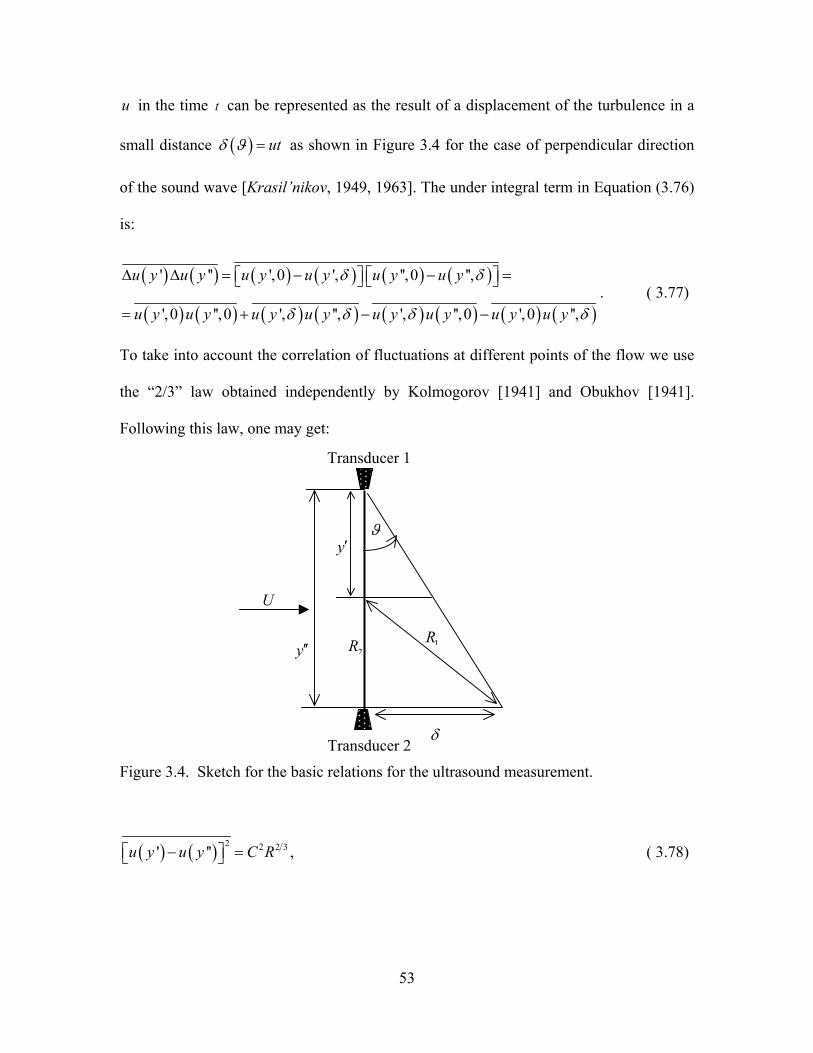
u in the time t can be represented as the result of a displacement of the turbulence in a
small distance as shown in Figure 3.4 for the case of perpendicular direction
of the sound wave [Krasil’nikov, 1949, 1963]. The under integral term in Equation (3.76)
is:
( ) utδ ϑ =
) ( )
( )
'
'',
',0
0 ',
u y
u y
=
= +
) 2 2 2' C R=
( ) ( ( ) ( ) ( )
( ) ( ) ( ) ( ) ( ) ( ) ( )
' ' ', '',0 '',
', 0 '', ', '', 0 ',0 '',
u y u y u y u y u y
u y u y u y u y u y u y u y
δ δ
δ δ δ
∆ ∆ − − =
− −. ( 3.77)
δ
To take into account the correlation of fluctuations at different points of the flow we use
the “2/3” law obtained independently by Kolmogorov [1941] and Obukhov [1941].
Following this law, one may get:
Transducer 1
Transducer 2
y′
δ
y′′
U
1R2R
ϑ
Figure 3.4. Sketch for the basic relations for the ultrasound measurement.
( ) ( 3' 'u y u y− , ( 3.78)
53
where constant C is the characteristic of turbulence having a dimension of 1 2/3 -1cm s×
and is a distance between the points and . However, based on the hypotheses of
isotropy of the turbulence the left side of Eq. (3.78) may be written as following
R 'y ''y
( ) ( ) ( )( ) ( ) ( )2 22 2/3 ' 2C R u y u y u y u y u y′′ ′ ′ ′′= − = −
. ( 3.79)
Based on the Figure 3.4 it is seen that
( ) ( )( ) ( ) ( )(1 , , ,0 ,0 , ,R R y y R y y )δ δ′ ′′ ′ ′′= = , ( 3.80)
( ) ( )( ) ( ) ( )(2 ,0 , ,0 , , ,R R y y R y y )δ δ′ ′′ ′ ′′= = , ( 3.81)
Simple geometry for small ϑ gives the following:
( 22 21 )R y yδ ′ ′′= + − , ( 3.82)
( 222 )R y y′′ ′= − . ( 3.83)
Now making use of the 2/3 law and equations (3.82), (3.83), one obtains for equation
(3.77):
( ) ( ) { } ( ) ( )( ){ }1/32 /3 22 2/3 2/3 2 21 2 0.5 2 2u y u y C R R C y y y y δ′ ′′ ′ ′′ ′ ′′∆ ∆ = − = − − − − + . ( 3.84)
Substitution of the Equation (3.84) into Equation (3.76), and integration yields the
following result:
22 2 5/3
2
1t C L constc
δ ∆ =
. ( 3.85)
in which the was determined experimentally in the works by Obukhov [1951] to be
equal to 3. Then, for the standard deviation the following expression takes place
[Krasil’nikov, 1949]
const
54
( )12 2 6
2
13t CLc
5σ δ = ∆ =
. ( 3.86)
Limits of Applicability of Geometrical Optics and Kolmogorov’s law
The theory of travel-time fluctuation, which we have just considered was based on
the equations of geometrical optics, statistical description of the turbulence and
Kolmogorov’s “2/3” law. The area of validity is defined by the following limits [Rytov et
al, 1978]
1. lελ <<
If there is a geometrical object with dimension lε is located on the propagation path of a
plane wave. At a distance from the obstacle we obtain its image with the same
dimension
L
lε . At the same time diffraction of the wave by the obstacle will occur. The
angle of divergence o the diffracted wave by the obstacle will be of order ~ / lα λ . At a
distance from the obstacle the size of the distracted bundle will be of order L
/ l~L Lα λ
/L l
. In order to neglect by diffraction effects it is necessary for the relation
lε ελ << to hold. Consequently, the second condition is
2. L lελ <<
Parameter Lλ is called the first Fresnel zone. The second condition applies restrictions
on the length of the travel path, i.e. 2 /criticalL L lε λ<< = . In the Chapter 4 it will be shown
based on our experimental data and supported by theoretical evidences [Rytov et al, 1978]
that for travel time variances in the presence of small diffraction effects, the ray acoustic
analytical approach may be considered as valid one for prediction of the travel time
55

variance. Consequently, the area of applicability of the ray acoustic approach for
calculation of travel time can be broader than the rigorous sufficient conditions define.
3.6 Travel-time Statistics of Acoustic Waves as an Experimental Tool for Diagnostic
of Turbulent Medium.
The fact that an acoustic wave carries some structural information regarding the
turbulent medium, after interaction, makes it possible to use the statistical characteristics
of the acoustic wave as a diagnostic tool to obtain some statistical information about the
medium. We consider isotropic homogeneous turbulence. The original goal of the
following theoretical derivations was firstly, to develop a methodology for determination
of correlation functions of turbulent velocity and sound speed fluctuations. Secondly, to
demonstrate quantitatively that effect of thermal fluctuations is as important as the effect
of velocity fluctuations on acoustic wave propagation. The ultrasonic flowmeter equation
is reconsidered, where the effects of turbulent velocity and sound speed fluctuations are
included [Andreeva and Durgin, 2001, 2002, 2003]. The result is an integral equation in
terms of correlation functions for travel time, turbulent velocity and sound speed
fluctuations.
We start with a classical equation for the flowmeter in the form it was derived in
equation (3.74) applied to waves traveling downstream shown in Figure 3.5
( ) sin ;'sin120 uUudyuU
ct
ucdyt
s s
+=++≈−
= ∫ ∫ ββ ' . ( 3.87)
In the experiment the only parameter that is measured is the travel time of ultrasound
pulses . Our intention is to construct a correlation function of the travel time using ( )t s
56
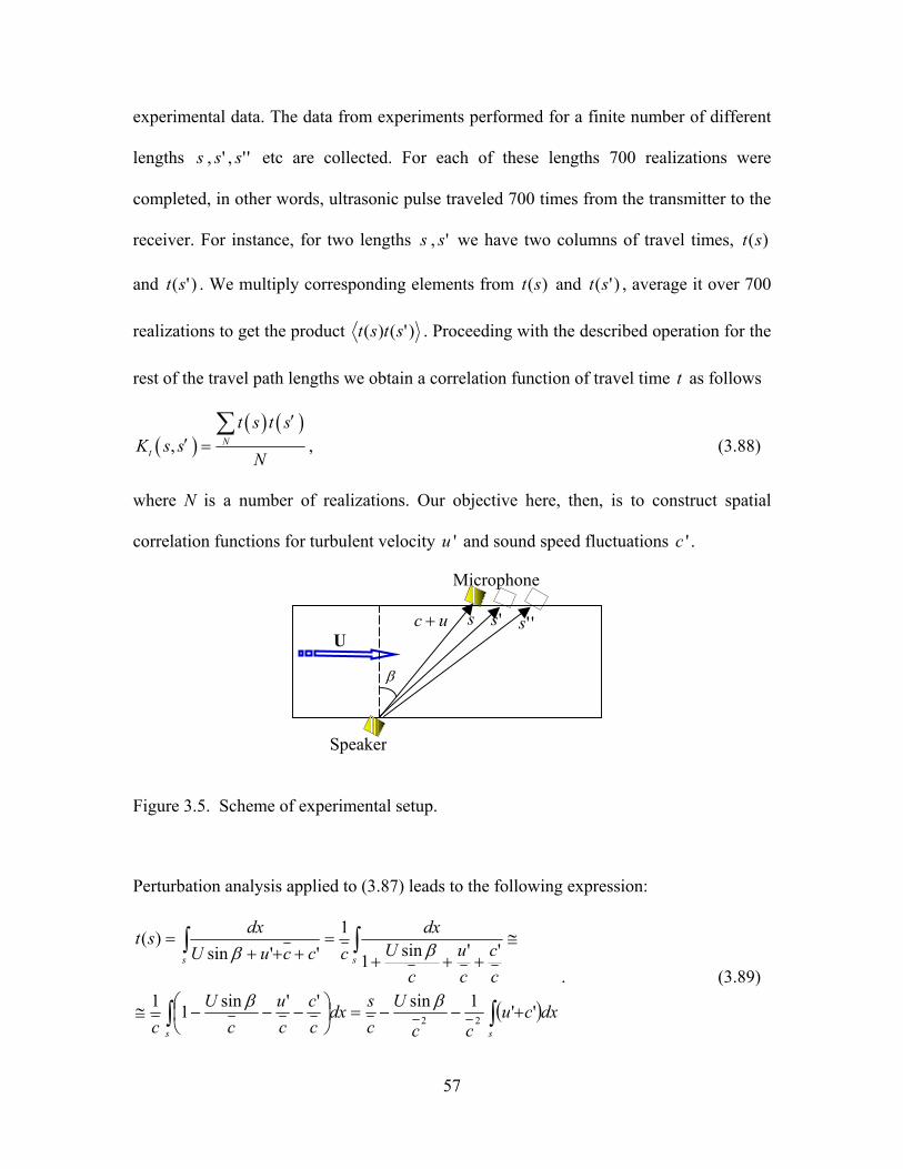
experimental data. The data from experiments performed for a finite number of different
lengths , , etc are collected. For each of these lengths 700 realizations were
completed, in other words, ultrasonic pulse traveled 700 times from the transmitter to the
receiver. For instance, for two lengths , we have two columns of travel times,
and . We multiply corresponding elements from and t , average it over 700
realizations to get the product
s
)
's ''s
s 's )(st
'(st )(st )'(s
)'()( stst . Proceeding with the described operation for the
rest of the travel path lengths we obtain a correlation function of travel time as follows t
( ), s′ N∑ t s
=
'u c
( )+ dxc'
∫
=s
1−
U +
β
+
c
dx
sin β
β
c
dx
sin2
β
U
sin
uc + s 's ''s
( ) ( )t
t sK s
N
′, (3.88)
where N is a number of realizations. Our objective here, then, is to construct spatial
correlation functions for turbulent velocity and sound speed fluctuations ' .
Speaker
Microphone
U
β
Figure 3.5. Scheme of experimental setup.
Perturbation analysis applied to (3.87) leads to the following expression:
∫ ∫
∫
−−=−−≅
≅++
=++
s s
s
uc
Ucsdx
cc
cu
c
cc
cu
cUcccu
st
'1''1
''sin1
1''
)(
2
.
(3.89)
57

Here we assumed that terms '/u c and '/c c are the same order infinitesimal compare to
unity. In order to construct the correlation function we introduce new variable:
( ) ( ) ( )ststst −=0. (3.90)
where angular brackets mean an operation of time averaging. Consequently,
( ) ( ) ( ) ( )0 02 2
1 1 ; s s
t s u c dx t s u c dxc c ′
′ ′ ′ ′ ′ ′= − + = − +∫ ∫ . (3.91)
Then,
( ) ( ) ( ) ( ) ( ) ( ){ }
( ) ( ) ( ) ( ){ }
0 04
4'
1
1 '
s s
s s
t s t s u x u x c x c x dxdxc
c x u x u x c x dxdxc
′
′ ′ ′ ′ ′ ′ ′= +
′ ′ ′ ′ ′ ′+ +
∫ ∫
∫ ∫
′ + . (3.92).
In the Equation (3.92) the first two terms represent the auto correlation functions of
turbulent velocity and sound speed fluctuations respectively. The second two terms are
cross correlation functions of turbulent velocity and sound speed fluctuations. In the
classical theory of isotropic, homogeneous turbulence cross correlation between velocity
and temperature, and, consequently between velocity and sound speed must necessarily
vanish everywhere. For the velocity measurement used here, the data were collected in
the isotropic region of flow, so that u and ' are not correlated. Consequently, the space
correlation function of time can be defined from the following equation
' c
( ) ( ) ( )( )
+== ∫ ∫
s scut dxdxxxKxxK
cssKstst
'''4
00 '',',1',)'()( .
(3.93)
It was observed experimentally [Sepri, 1976] that the velocity statistics were identical
within experimental limits with and without grid heating. It is important to emphasize
that the space correlation function alone can be defined based on data from ( , ')uK x x
58

room temperature experiments. Then, data from heated air experiments can be used to
identify knowing that is taken unchanged from the room temperature
experiment and .
( , ')cK x x
K
( , ')uK x x
( ', sst
λ
l Lλ
2 20 0/l L Lλ λ< < Dif− ction region
)
3.7 Parabolic Equation Approximation
As it was mentioned in section 3.2 the closed system of linearized equations (3.46-
3.49) is rather complicated. One of the simplifications, the ray acoustics approach, was
discussed and applied in the previous subsection. Nevertheless, scientists have been
trying to reduce the system to a single equation, which would be simpler then for analysis
then the starting system. There are various approximations or assumptions about a
moving medium in use, such as the Andreev-Rusakov-Blokhintzev equation for
irrotational flow, Monin’s equation for dry air, Goldstein equation for sound waves in
parallel shear flow, equation for acoustical and internal gravity waves in a stratified
moving medium, derived by Ostashev [1997], parabolic equation method approximation.
These are only a few approximations existing up to date. Because of the specifics of our
research work, namely, when limits of applicability of ray acoustics theory are violated,
i.e.
1. lε >>
2. ε <<
3. / fra
If this is the case, then effects of small diffractions must be taken into account. The
parabolic equation exhibits a perfect fit for this situation. The parabolic equation method
59
is very powerful method in the theory of wave propagation. We do not intend to rederive
the parabolic equations, but rather reproduce it in the form it was derived by Rytov [1978]
from the Helmholtz equation
( )( ) 0~12 =++∆ urku ε ( 3.94)
where is the wave field, is the wave number and u k ( )[ ] εεεε /~ −= r reflects the
relative fluctuations of dielectric permeability [Rytov, 1978]. We consider a plane wave
propagating along the direction x . Let u be such that ( )ikxA exp0u = . We assume that l
is the smallest correlation length. We study only the high-frequency propagation, .
This condition allows us to neglect, explicitly, the backscattered parts of the wave in the
Helmholtz equation. It is useful to express the solution of equation (3.94) in the following
form:
1>kl
),( ),exp(),(),( zyikxxvxu == rrr (3.95)
Here is complex wave amplitude. Substitution of the equation (3.95) in (3.94)
leads to the parabolic wave equation [Rytov, 1978]
( r,xv )
( ) 0,~2 22
2
2
2
=+∂∂
+∂∂
+∂∂ vxk
zv
yv
xvik rε . (3.96)
In a turbulent medium there are inhomogeneities with different scales, which are greater
than the inner scale of turbulence, l , and smaller than the outer scale, : . It
has been shown, [Ostashev, 1997] that in a turbulent medium the range of applicability of
the parabolic equation is given by inequality
0 0L 00 llL >>
λ>>0L . The parabolic equation cannot be
solved exactly in a general case. As the velocity fluctuations are small
( 21, where = ε εσ σ ε<< ), the parabolic equation can be solved using a perturbation
60
method or, so called, the first order Rytov approximation. The method of perturbations is
perfectly suited for investigating such wave parameters as the phase difference and the
log-amplitude. Introducing the complex amplitude ( )r,xv as follows
( )r,x
,y z
∂+ ∆
rrr (exp),(ln),((exp),( 00
0 AAxAxiAxv Φ=
+= φ . (3.97)
It follows from equation (3.97) that ( )0/ln Av=Φ . Here kxW −=φ - phase difference,
and ( ) χ≡0/ln AA - log-amplitude. Substitution (3.97) into (3.96) leads to the equation for
the complex phase.
( )2 2
2 22) , 0, ik k x 22 (
x y zε⊥ ⊥ ⊥ ⊥
∂Φ ∂ ∂ ∂+ ∆ Φ + ∇ Φ + = ∇ = = +
∂ ∂r%
∂ ∂ ∂. (3.98)
Solution can be expressed as a power series
21 2 ...ε εσ σΦ = Φ + Φ + . (3.99)
Substituting into the parabolic equation and keeping terms up to second order gives:
( )211
222 1
2 ,
2 (
ik k xx
ikx
ε⊥
⊥ ⊥
∂Φ+ ∆ Φ = −
∂
∂Φ+ ∆ Φ = − ∇ Φ
∂
r%
)
. (3.100)
The problem of phase and log-amplitude fluctuations is considered using these equations.
Equations (3.100) are solvable and valid only when the small fluctuations regime holds
[Rytov, 1997] i.e.
2 21 or k 2
1ε εσ λ⊥ ⊥∇ Φ << ∇ Φ << σ . (3.101)
Consequently, the parabolic approximation neglects the backscattered part of the wave.
Rytov’s approximation says that the wave field u is not different from the
61
monochromatic wave , which propagates in the background homogeneous
medium. Using the Rytov approximation, explicit equations for the phase of a sound
wave and its log-amplitude
)exp(ikx
Φ
χ are obtained.
2 2
2 21 sinF
F
K KKK K
2 2
2 21 sinF
F
K KKK K
e k her
1/3
The equations for the variances of the log-amplitude and phase fluctuations of a
plane wave in a moving random medium derived by means of Rytov method, have the
following form [Ostashev, 1997]
2 22
0
(0, )2 effk xπχ
∞ = − Φ
∫ , (3.102) K dK
2 22
0
(0, )2 effk xπφ
∞
= + Φ∫ . (3.103) K dK
Here is a wave number. Note, that 2 / , wherFK k x= 2 / , w e F F FK L Lπ λ= =
is the scale of the first Fresnel zone. effΦ is the three-dimensional spectral density of the
random field ε and is called an effective function. The equations for statistical moments
of φ and χ are valid for an arbitrary spectra of inhomogeneities in moving random
medium. For our purpose we use Kolmogorov and Gaussian spectra of medium
inhomogeneities. The Markov approximation for the effective spectral density is
[Ostashev, 1997]
x
2 1(0, )eff effK AC K −Φ = , (3.104)
where A is a numerical coefficient, and C is, so called, effective structure parameter,
given by
2eff
22 2
2
223
veff
CC Ccε
ε
= + . (3.105)
62
Here 2Cε and are the structure parameters of the random field [Ostashev, 1997].
Substituting (3.104) into (3.102) results into formula for the variance of the log-amplitude
fluctuations for a plane wave:
2vC
2
2 2 72
220.0773
vCC kcε
ε
χ
= +
/ 6 11/ 6x . (3.106)
Substitution of (3.104) for the Kolmogorov spectrum into the integral for phase
fluctuations results in a divergent integral. Therefore, 2φ can be determined neither for
a plane nor for a spherical wave [Ostashev, 1997]. The formula for an effective spectral
density for the Gaussian spectrum is
(2 2 23
23/ 2 2
0
(0, ) exp / 48
veff
K llKcε
ε
σσπ
Φ = + −
)2 2K l . (3.107)
For plane wave propagation, the variances of the log-amplitude and phase fluctuations
are [Ostashev , 1997]
22 22 2
20
4arctan arctan1 18
vk lx D DD Dε c
σπχ σ = − + −
, (3.108)
22 22 2
20
4arctan arctan1 18
vk lx D DD Dε c
σπφ σ = + + +
. (3.109)
In equations. (3.108) and (3.109) ( )24 /D x kl= is the wave parameter used in the theory
of waves in random media [Chernov, 1961] and vσ is a sound scattering cross section due
to the velocity fluctuations. Equations (3.108) and (3.109) in their original version were
given for [Rytov, 1978]. 2 0vσ =
63
Chapter 4. Experimental Apparatus
The experiment was performed in a low-speed tunnel. The turbulence was produced
by a grid. The ultrasonic technique was employed for diagnostic and determination of the
statistics of grid-generated turbulence. The following chapter is devoted to the description
of the experimental apparatus: wind tunnel, grid, ultrasonic system and data acquisition
and analysis system. The major steps of the performance of ultrasonic measurement
system with a discussion of each component of the system, namely, ultrasonic flowmeter,
Data Acquisition Cards, LabVIEW software and characteristics of each component are
summarized in this chapter. This chapter is concluded with description of LabVIEW Vi -
the block diagram of the OSCOPE module, responsible for driving data acquisition cards,
and analyzing acquired.
4.1 Wind Tunnel
The experiments were carried out in a wind tunnel of length with a
rectangular test section. The AEROLAB low turbulence, low speed,
research tunnel is of the Eiffel or Open Circuit type. The airspeed is infinitely variable
from 0 to 80 mph. The tunnel achieves a high energy ratio through its large contraction
ratio, 16:1, its small angle diffuser and efficient fan system. The high energy ratio is
45.25′′
11.75 x 11.62′′′′
64
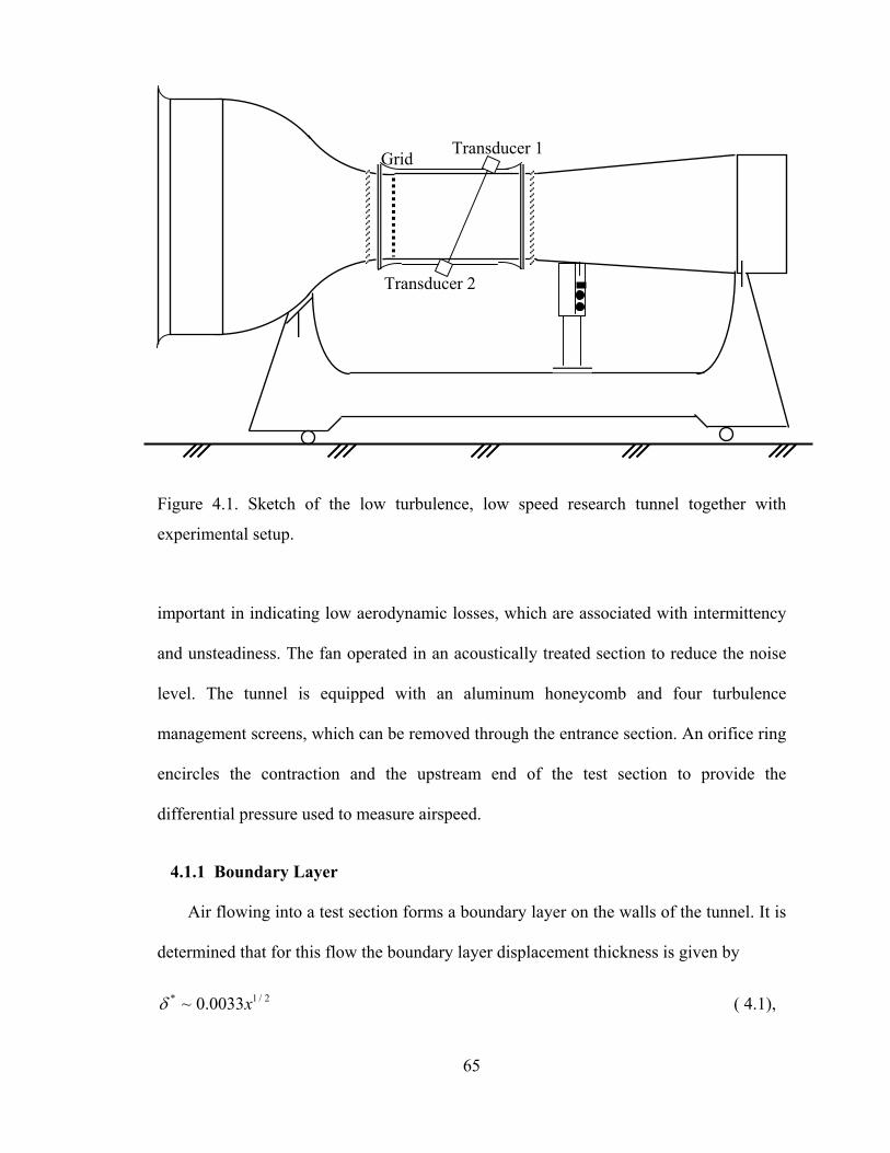
Transducer 2
Transducer 1Grid
Figure 4.1. Sketch of the low turbulence, low speed research tunnel together with
experimental setup.
important in indicating low aerodynamic losses, which are associated with intermittency
and unsteadiness. The fan operated in an acoustically treated section to reduce the noise
level. The tunnel is equipped with an aluminum honeycomb and four turbulence
management screens, which can be removed through the entrance section. An orifice ring
encircles the contraction and the upstream end of the test section to provide the
differential pressure used to measure airspeed.
4.1.1 Boundary Layer
Air flowing into a test section forms a boundary layer on the walls of the tunnel. It is
determined that for this flow the boundary layer displacement thickness is given by
2/1* 0033.0~ xδ ( 4.1),
65
where x is a distance downstream the tunnel. It can be estimated that the maximum
displacement thickness corresponding to the measurements taken at
downstream the grid. Consequently, the effect of boundary layer results in 7%
change in mean velocity U and in 0.05% in the total velocity which is a sum of the
velocity of a sound wave and a mean velocity.
m0031.0~*δ
mx .0= 89
4.2 The Grid
The turbulent velocity and turbulent temperature fluctuations are simultaneously
generated by a bi-planar grid composed of 18 round chromalox heating rods, model
TSSM 14XX [Sreenivasan, 1980], placed at the entrance of the test section. To insure
uniformity of the grid, the heating rods were inserted in hollow aluminum rods with
diameter of positioned 10.25′′ ′′ between centers. The mesh, M, was therefore 1′′ and the
grid solidity was 0.64. The rods are all heated evenly; hence the thermal mesh size is
equal to that of the momentum. The grid power was regulated by variable transformator.
The heated grid surface temperature was measured by thermocouple, while mean air
temperature of the tunnel flow is measured by thermometer. Overall, the grid structure
resembles the features of the grid used by Sreenivasan, who performed measurements of
turbulence decay in the wind tunnel with similar geometry. It has been experimentally
verified [Sreenivasan, 1980; Yeh and van Atta, 1973; Sepri, 1976; Mohammed and
LaRue, 1990] that this particular choice of the grid geometry together with geometry of
the tunnel, insures that in the region '25 '' 40 '− the turbulence can be considered
approximately isotropic.
66
4.3 Description of the Ultrasonic System
4.3.1 Transit Time Flowmeters
Measurements were performed by means of an ultrasonic system. The transducer is
one of the most critical components of any ultrasonic system. A transducer is any device
that converts one form of energy to another. An ultrasonic transducer converts electrical
energy to mechanical energy, in the form of sound, and vice versa. The main components
are the active element, backing, and wear plate as shown in Figure 4.2. The active
element, which is piezo or ferroelectric material, converts electrical energy such as an
excitation pulse from a flaw detector into ultrasonic energy. The backing is usually a
highly attenuative, high density material that is used to control the vibration of the
transducer by absorbing the energy radiating from the back face of the active element.
The basic purpose of the transducer wear plate is to protect the transducer element from
the testing environment. In the case of contact transducers, the wear plate must be a
durable and corrosion resistant material in order to withstand the wear caused by use on
materials such as steel. For our application we use Low Frequency Narrowband
Transducers, meant for use in pairs for through transmission in materials with working
frequency of 100KHz. The ultrasonic flowmeter utilizes two transducers functioning both
as a transmitter and as a receiver, as shown in Figure 4.3. The principle is based on
modification of the time of flight of the ultrasound by the fluid velocity along the line of
the flight path between the two transducers. The method results in measurement of very
short time delays of about a few nanoseconds.
67

connector
Electrodes Wear plate
Active element
Backing
Inner sleeve
Electrical leads
Electrical housing
Figure 4.2. Design characteristics of an ultrasonic transducer
A great deal of attention should be paid to selecting the proper transducer for the
application. The optimal choice of ultrasonic frequency depends on two factors.
Consistent with absorption factor and minor fluid turbulence the highest practical
frequency should be used. The lower limit is related to the vortex size, which, in turn, is
related to the size of the vortex-generating strut [Lynnworth, 1989]
1/ ; / , ( ) 2k L ck c f f Hzλ πω= = = = ( 4.2).
Transducer 2
Transducer 1
Figure 4.3. Transit-time ultrasonic flowmeter.
68
4.3.2 Data Acquisition and Analysis System
Measurement devices, such as general-purpose data acquisition (DAQ) devices and
special-purpose instruments, are concerned with the acquisition, analysis, and
presentation of measurements and other data you acquire. Acquisition is the means by
which physical signals, such as voltage, current, pressure, and temperature, are converted
into digital formats and brought into the computer. Popular methods for acquiring data
include plug-in DAQ and instrument devices. Data analysis transforms raw data into
meaningful information. This can involve such things as curve fitting, statistical analysis,
frequency response, or other numerical operations. DAQ devices are devices that connect
to the computer allowing the user to retrieve digitized data values. These devices
typically connect directly to the computer’s internal bus through a plug-in slot. With
DAQ devices, the hardware only converts the incoming signal into a digital signal that is
sent to the computer as shown in Figure 4.4. The DAQ device does not compute or
calculate the final measurement. That task is left to the software that resides in the
computer. The same device can perform a multitude of measurements by simply
changing the software application that is reading the data. Before a computer-based
system can measure a physical signal, a sensor or signal conditioning must convert the
physical signal into an electrical one, such as voltage or current. The software controls
the DAQ system by acquiring the raw data, analyzing the data, and presenting the results.
The role of software is crucial. Software takes the raw data and presents it in a form of a
graph, chart etc. The software controls the DAQ system, telling the DAQ device when to
acquire data. DAQ software includes drivers and application software. Drivers are unique
to the type of the device and include the set of commands the device accepts.
69

Software
Plug-in DAQ board
Conditioned Signal
Signal Conditioning
Transducers
Figure 4.4. DAQ System Components
Application software (in our case LabVIEW) sends the commands to the drivers, such as
acquire a transducer reading and return the reading, then displays and analyzes the data
acquired. Lab VIEW includes a set of Vis that let us configure, acquire data from and
send data to DAQ devices. LabVIEW DAQ Vis makes calls to the NI-DAQ Application
Program Interface (API). The NI-DAQ API contains the tools and basic functions that
interface to DAQ hardware. Lab VIEW instrument drivers simplify instrument
programming to high-level commands, so there is no need to learn the low-level
instrument-specific syntax needed to control the instrument. Figure 4.5 shows the
relationship between LabVIEW, driver software, and measurement hardware.
70
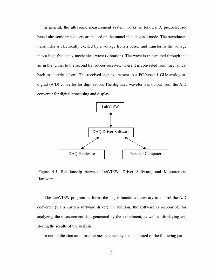
In general, the ultrasonic measurement system works as follows. A piezoelectric-
based ultrasonic transducers are placed on the tunnel in a diagonal mode. The transducer-
transmitter is electrically excited by a voltage from a pulser and transforms the voltage
into a high frequency mechanical wave (vibration). The wave is transmitted through the
air in the tunnel to the second transducer-receiver, where it is converted from mechanical
back to electrical form. The received signals are sent to a PC-based 1 GHz analog-to-
digital (A/D) converter for digitization. The digitized waveform is output from the A/D
converter for digital processing and display.
Personal Computer DAQ Hardware
DAQ Driver Software
LabVIEW
Figure 4.5. Relationship between LabVIEW, Driver Software, and Measurement
Hardware
The LabVIEW program performs the major functions necessary to control the A/D
converter (via a custom software driver). In addition, the software is responsible for
analyzing the measurement data generated by the experiment, as well as displaying and
storing the results of the analysis.
In our application an ultrasonic measurement system consisted of the following parts:
71
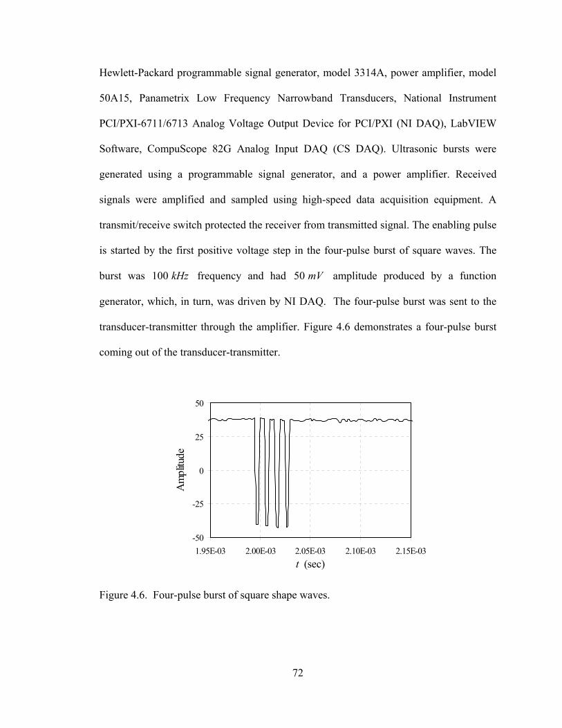
Hewlett-Packard programmable signal generator, model 3314A, power amplifier, model
50A15, Panametrix Low Frequency Narrowband Transducers, National Instrument
PCI/PXI-6711/6713 Analog Voltage Output Device for PCI/PXI (NI DAQ), LabVIEW
Software, CompuScope 82G Analog Input DAQ (CS DAQ). Ultrasonic bursts were
generated using a programmable signal generator, and a power amplifier. Received
signals were amplified and sampled using high-speed data acquisition equipment. A
transmit/receive switch protected the receiver from transmitted signal. The enabling pulse
is started by the first positive voltage step in the four-pulse burst of square waves. The
burst was 100 frequency and had 50 amplitude produced by a function
generator, which, in turn, was driven by NI DAQ. The four-pulse burst was sent to the
transducer-transmitter through the amplifier. Figure 4.6 demonstrates a four-pulse burst
coming out of the transducer-transmitter.
kHz mV
-50
-25
0
25
50
1.95E-03 2.00E-03 2.05E-03 2.10E-03 2.15E-03t (sec)
Am
plitu
de
Figure 4.6. Four-pulse burst of square shape waves.
72
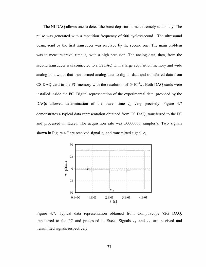
The NI DAQ allows one to detect the burst departure time extremely accurately. The
pulse was generated with a repetition frequency of 500 cycles/second. The ultrasound
beam, send by the first transducer was received by the second one. The main problem
was to measure travel time t with a high precision. The analog data, then, from the
second transducer was connected to a CSDAQ with a large acquisition memory and wide
analog bandwidth that transformed analog data to digital data and transferred data from
CS DAQ card to the PC memory with the resolution of . Both DAQ cards were
installed inside the PC. Digital representation of the experimental data, provided by the
DAQs allowed determination of the travel time t very precisely. Figure 4.7
demonstrates a typical data representation obtained from CS DAQ, transferred to the PC
and processed in Excel. The acquisition rate was 50000000 samples/s. Two signals
shown in Figure 4.7 are received signal e and transmitted signal .
n
95 10 s−⋅
n
1 2e
-50
-25
0
25
50
0.E+00 1.E-03 2.E-03 3.E-03 4.E-03t (s)
Am
plitu
de
1e
2
e
Figure 4.7. Typical data representation obtained from CompuScope 82G DAQ,
transferred to the PC and processed in Excel. Signals e and are received and
transmitted signals respectively.
1 2e
73
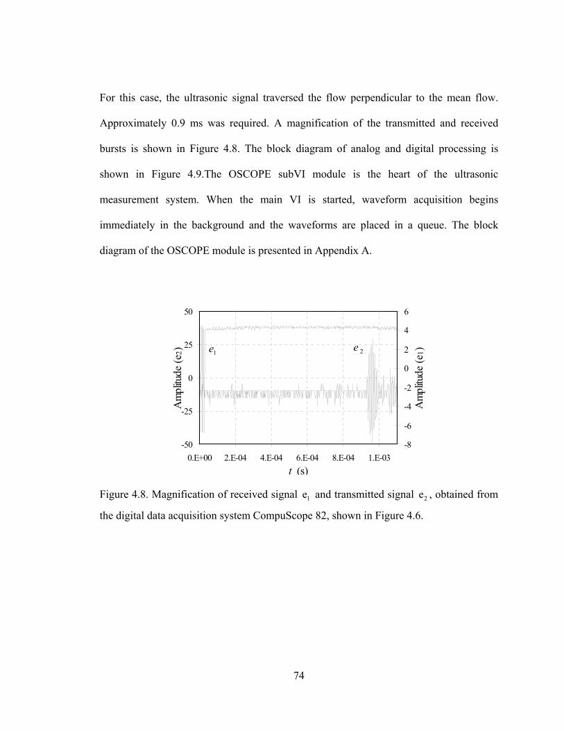
For this case, the ultrasonic signal traversed the flow perpendicular to the mean flow.
Approximately 0.9 ms was required. A magnification of the transmitted and received
bursts is shown in Figure 4.8. The block diagram of analog and digital processing is
shown in Figure 4.9.The OSCOPE subVI module is the heart of the ultrasonic
measurement system. When the main VI is started, waveform acquisition begins
immediately in the background and the waveforms are placed in a queue. The block
diagram of the OSCOPE module is presented in Appendix A.
-50
-25
0
25
50
0.E+
Am
plitu
de (e
2) 2
4
6
e 1)1e 2e
Figure 4.8. Magnificati
the digital data acquisit
00 2.E-04 4.E-04 6.E-04 8.E-t (s)
on of received signal e and tra
ion system CompuScope 82, sho
1
74
04 1.E-03-8
-6
-4
-2
0
Am
plitu
de (
nsmitted signal e , obtained from
wn in Figure 4.6.
2
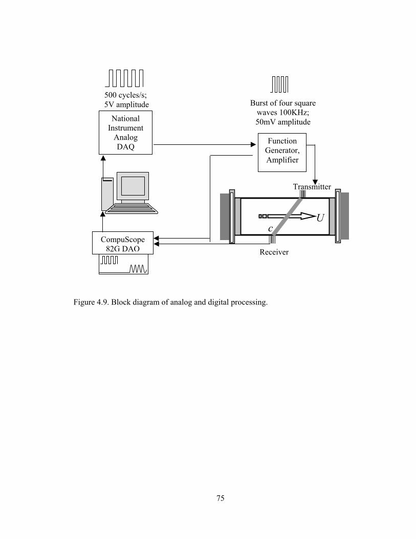
Uc
Receiver
Transmitter
Burst of four square waves 100KHz; 50mV amplitude
Function Generator, Amplifier
CompuScope 82G DAQ
500 cycles/s; 5V amplitude
National Instrument
Analog DAQ
Figure 4.9. Block diagram of analog and digital processing.
75
Chapter 5. Experimental Results and Discussion
In this chapter we present the most important aspect of the dissertation: application
of the travel-time ultrasonic technique for data acquisition in a grid-generated turbulence
and analysis of the experimental data.
5.1 Application of Travel-time Ultrasonic Techniques for Data Acquisition
We consider here a locally isotropic turbulent flow, which can be approximately
generated by introducing a grid into a uniform flow. At a sufficient distance downstream
from the grid the flow becomes locally isotropic and a power law spectral representation
is applicable. Studies that permit identification of the downstream position where the
flow be considered nearly homogeneous and locally isotropic are described in detail by G
Corrsin; Uberoi and Wallis [1967], Comte-Bellot and Corrsin [1971] Mohamed and
LaRue [1990]. In order to collect experimental data in nearly isotropic and homogeneous
portions of flow, the locations of transducers as well as mean flow speed were chosen
using the criteria established by Mohamed and LaRue. Specifically, experimental data
were collected in the portion of the test section. The specific grid structure as
well as the tunnel geometry were essentially the experimental setups used by previous
investigators to insure that turbulence level and other statistical characteristics of the
turbulence were the same as measured by Yeh and van Atta [1973], Sepri [1976],
25 '' 42 ''−
76
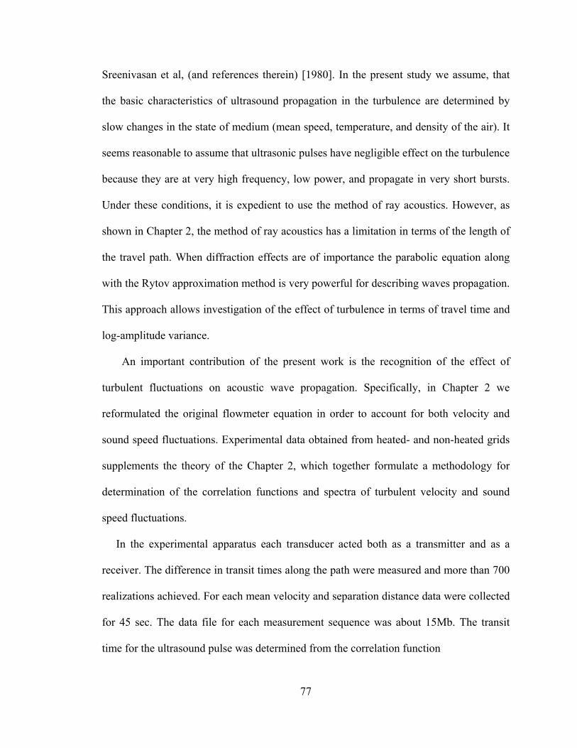
Sreenivasan et al, (and references therein) [1980]. In the present study we assume, that
the basic characteristics of ultrasound propagation in the turbulence are determined by
slow changes in the state of medium (mean speed, temperature, and density of the air). It
seems reasonable to assume that ultrasonic pulses have negligible effect on the turbulence
because they are at very high frequency, low power, and propagate in very short bursts.
Under these conditions, it is expedient to use the method of ray acoustics. However, as
shown in Chapter 2, the method of ray acoustics has a limitation in terms of the length of
the travel path. When diffraction effects are of importance the parabolic equation along
with the Rytov approximation method is very powerful for describing waves propagation.
This approach allows investigation of the effect of turbulence in terms of travel time and
log-amplitude variance.
An important contribution of the present work is the recognition of the effect of
turbulent fluctuations on acoustic wave propagation. Specifically, in Chapter 2 we
reformulated the original flowmeter equation in order to account for both velocity and
sound speed fluctuations. Experimental data obtained from heated- and non-heated grids
supplements the theory of the Chapter 2, which together formulate a methodology for
determination of the correlation functions and spectra of turbulent velocity and sound
speed fluctuations.
In the experimental apparatus each transducer acted both as a transmitter and as a
receiver. The difference in transit times along the path were measured and more than 700
realizations achieved. For each mean velocity and separation distance data were collected
for 45 sec. The data file for each measurement sequence was about 15Mb. The transit
time for the ultrasound pulse was determined from the correlation function
77

( ) ( )12 1 2( )K t e t e tτ= + , ( 5.1)
where is a cross correlation function of received and transmitted waves and
shown in Figure 4.7. By definition
)t(K12 1e
2e
( ) ( ) ( )12 1 2 1 20
( ) , ,K t e t e t p e e t dtτ∞
= +∫ , ( 5.2)
where ( 1 2, , )p e e t is a probability density function. However, assuming the process to be
ergodic, spatial averaging may be replaced by averaging over the time:
( ) ( )12 1 20
1( )T
K t e t e t dtT
τ= +∫ . ( 5.3)
Hence, the travel time may be determined as nt
12 12max ( ) ( )nK t K t= . ( 5.4)
The numerical computation of the cross correlation function involves the computation of
average products among the sample data values [Bendat and Piersol, 1971]. Namely, we
consider data values {N } , 1, 2,...,nx n = N sampled at equally spaced time intervals dt
from a transformed record ( ) ( )x t x ndt= . The cross correlation function of ( )x t can be
estimated from the sample values at the time delay by rdt
( )121
1 , 0,1,2,...,N r
n n rn
K rdt x x r mN r
−
+=
= =− ∑ . ( 5.5)
The number of real multiply-add operations required to compute the cross correlation
estimate is approximately , assumingNm N m<<
12
. The numerical code, which was used
to calculate the cross correlation function K included module CCF from IMSL Fortran
78
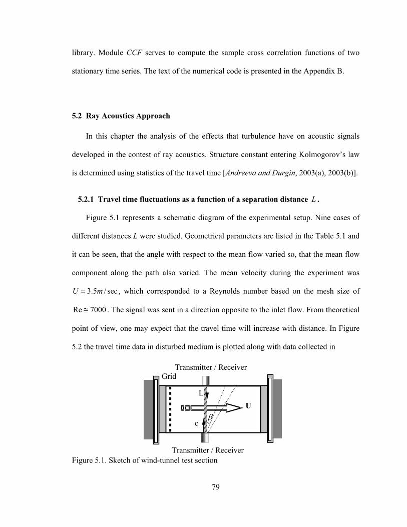
library. Module CCF serves to compute the sample cross correlation functions of two
stationary time series. The text of the numerical code is presented in the Appendix B.
5.2 Ray Acoustics Approach
In this chapter the analysis of the effects that turbulence have on acoustic signals
developed in the contest of ray acoustics. Structure constant entering Kolmogorov’s law
is determined using statistics of the travel time [Andreeva and Durgin, 2003(a), 2003(b)].
5.2.1 Travel time fluctuations as a function of a separation distance . L
Figure 5.1 represents a schematic diagram of the experimental setup. Nine cases of
different distances L were studied. Geometrical parameters are listed in the Table 5.1 and
it can be seen, that the angle with respect to the mean flow varied so, that the mean flow
component along the path also varied. The mean velocity during the experiment was
, which corresponded to a Reynolds number based on the mesh size of
. The signal was sent in a direction opposite to the inlet flow. From theoretical
point of view, one may expect that the travel time will increase with distance. In Figure
5.2 the travel time data in disturbed medium is plotted along with data collected in
3.5 / secU m=
Re 7000≅
Figure 5.1. Sketch of wind-tunnel test section
U
Transmitter / Receiver
Transmitter / Receiver
β
c
Grid
L
79

undisturbed medium and compared with theoretical estimation of the travel time without
taking into account the effect of turbulence, namely, ( ) sintheoretical
t L c U β= − . Figure 5.3
demonstrates well-expected result of significant decrease of mean travel time in presence
β (deg) 0 5 10 15 20 25 30 35 40
L (m) 0.33 0.3335 0.3395 0.3483 0.3603 0.3758 0.3955 0.42 0.45
Table 5.1. Geometrical parameters.
of turbulence. The decrease due to turbulence is 5% or greater. The uncertainty in
measurements of the ambient temperature is at most 3.5%, which would introduce an
uncertainty in the mean travel time determination of only 0.2%. Similarly, the uncertainty
in measurements of the travel distance 0.3%, which would introduce an uncertainty in the
measurement of the travel time of approximately 0.3%. Figure 5.3 demonstrates the
travel time standard deviation as a function of traveled distance. The result obtained by
Kolmogorov and Obukhov predicts that the standard deviation should increase in
proportion to the square root of a distance, which is depicted by the solid line. Therefore,
the experimental data is plotted together with 1 2L curve in order to verify that the
standard deviation obtained experimentally is indeed proportional to 1 2L . Although the
standard deviation is increasing with distance, the scattering of the data can be clearly
seen. The scattered data must be interpreted with some caution and may not be
inconsistent with the theoretical analysis, but rather may be due to the uncertainty of the
measurements, which were found to be around 20%.
80
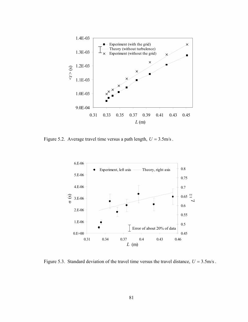
9.0E-04
1.0E-03
1.1E-03
1.2E-03
1.3E-03
1.4E-03
0.31 0.33 0.35 0.37 0.39 0.41 0.43 0.45L (m)
<t>
(s)
Experiment (with the grid)Theory (without turbulence)Experiment (without the grid)
Figure 5.2. Average travel time versus a path length, m/s5.3=U .
0.E+00
1.E-06
2.E-06
3.E-06
4.E-06
5.E-06
6.E-06
0.31 0.34 0.37 0.4 0.43 0.46L (m)
(s)
0.45
0.5
0.55
0.6
0.65
0.7
0.75
0.8
L1/
2
Experiment, left axis Theory, right axis
σ
Error of about 20% of data
Figure 5.3. Standard deviation of the travel time versus the travel distance, U . m/s5.3=
81

5.2.2 Transit Time Fluctuations as a Function of the Mean Velocity U .
For this case we used two transducers placed at a distance from each other with
the direction of mean flow perpendicular to L. The Reynolds number based on the mesh
size
L
M varied from 4016 to 20080. Following the procedure described in the foregoing
section the cross correlation function of two signals for U was
obtained and is shown in Figure 5.4. After calculation of the travel time t for each
sample using formula we calculated the averaged travel time
12K 21 e,e 4 (m/sec)=
t< > and deviation of the
transit time σ for each velocity.
-0.3
-0.2
-0.1
0.0
0.1
0.2
0.3
0.0E+00 2.0E-04
K12
(s2 )
Figure 5.4. Correlation function ( )12K t
tfunction corresponds to the travel time
Averaged travel time and deviation of
carry the most information about exp
substantial decrease in t as mean velo
for a standard deviation, σ , theory pred
travel time t
4.0E-04 6.0E-04 8.0E-04 1.0E-03t (s)
of two waves. Maximum value of the correlation
.
the travel time are two crucial parameters that
erimental data. As expected, Figure 5.5 shows
city increases. As it was stated in the section 3.5,
icts a dependence of ( . Figure 5.6 )5/ 6U t< >
82
9.44E-04
9.45E-04
9.46E-04
9.47E-04
9.48E-04
0 1 2 3 4 5 6 7 8 9 10U (m/s)
<t>(
s)
Averaged travel time with the gridAveraged travel time without the mean flow
Figure 5.5. Averaged travel time as a function of the mean velocity, 0 m,33.0 == βL .
0.E+00
1.E-02
2.E-02
3.E-02
4.E-02
1.5E-03 6.5E-03 1.2E-02U<t> (m)
(U<
t>)5/
6
0.E+00
4.E-05
8.E-05
1.E-04
2.E-04
2.E-04
(s)
Theory, left axis Experiment, right axis
Error of about 20% of data
Figure 5.6. Standard deviation of the travel time versus mean velocity, 0 m,33.0 == βL .
illustrates that experimental results are in fairly good accordance with theoretical
predictions, namely, standard deviation is proportional to . After validation of ( 5/ 6U t< >)
our experimental results we may determine the turbulent constant from equation (3.85) C
83
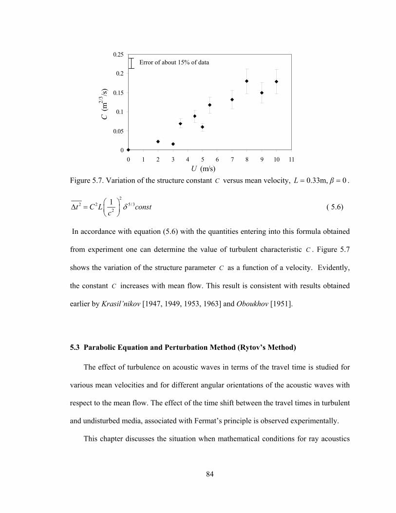
0
0.05
0.1
0.15
0.2
0.25
0 1 2 3 4 5 6 7 8 9 10 11U (m/s)
C (m
2/3 /s)
Error of about 15% of data
Figure 5.7. Variation of the structure constant C versus mean velocity, 0 m,33.0 == βL .
22 2 5/3
2
1t C L constc
δ ∆ =
( 5.6)
In accordance with equation (5.6) with the quantities entering into this formula obtained
from experiment one can determine the value of turbulent characteristic . Figure 5.7
shows the variation of the structure parameter as a function of a velocity. Evidently,
the constant increases with mean flow. This result is consistent with results obtained
earlier by Krasil’nikov [1947, 1949, 1953, 1963] and Oboukhov [1951].
C
C
C
5.3 Parabolic Equation and Perturbation Method (Rytov’s Method)
The effect of turbulence on acoustic waves in terms of the travel time is studied for
various mean velocities and for different angular orientations of the acoustic waves with
respect to the mean flow. The effect of the time shift between the travel times in turbulent
and undisturbed media, associated with Fermat’s principle is observed experimentally.
This chapter discusses the situation when mathematical conditions for ray acoustics
84
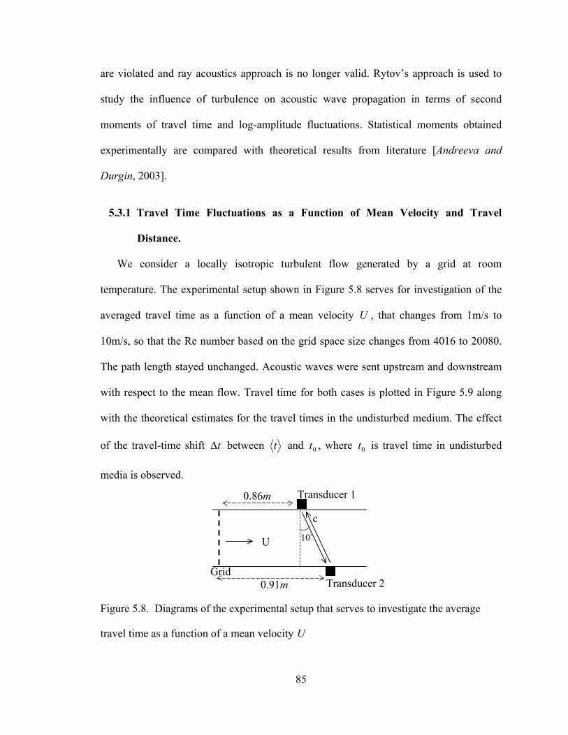
are violated and ray acoustics approach is no longer valid. Rytov’s approach is used to
study the influence of turbulence on acoustic wave propagation in terms of second
moments of travel time and log-amplitude fluctuations. Statistical moments obtained
experimentally are compared with theoretical results from literature [Andreeva and
Durgin, 2003].
5.3.1 Travel Time Fluctuations as a Function of Mean Velocity and Travel
Distance.
We consider a locally isotropic turbulent flow generated by a grid at room
temperature. The experimental setup shown in Figure 5.8 serves for investigation of the
averaged travel time as a function of a mean velocity U , that changes from 1m/s to
10m/s, so that the Re number based on the grid space size changes from 4016 to 20080.
The path length stayed unchanged. Acoustic waves were sent upstream and downstream
with respect to the mean flow. Travel time for both cases is plotted in Figure 5.9 along
with the theoretical estimates for the travel times in the undisturbed medium. The effect
of the travel-time shift between t∆ t and t , where is travel time in undisturbed
media is observed.
0 0t
10o
Transducer 2
Transducer 1
Grid 0.91m
0.86m
c
U
Figure 5.8. Diagrams of the experimental setup that serves to investigate the average
travel time as a function of a mean velocity U
85

Due to the fast path effect, the effective velocity is higher than the mean velocity of the
medium. Indeed, 0tt ≤ and 0t
XtX
≥ [Iooss, 2000]. The experimental setup shown in
Figure 5.10 serves to illustrate the influence of the travel distance varying from 0.33m to
0.45m. The mean velocity was unchanged, 3.5 m/s. Another interesting effect of acoustic
wave propagation is the linear increase of travel time variance with distance [Chernov,
1960]. Nonlinear effects become apparent at a certain propagation distances both in the
numerical experiments by Karweit et al, [1991] and in the work by Iooss et al, [2000].
9.70E-04
9.73E-04
9.76E-04
9.79E-04
9.82E-04
9.85E-04
9.88E-04
9.91E-04
9.94E-04
0 1 2 3 4 5 6 7 8 9 1
U (m/s)
<t>
(s)
0
Downstram propagation in turbulent meadia, experimentUpstream propagation in turbulent media, experimentDownstream propagation in undisturbed media, theoryUpstream propagation in undisturbed media, theory
Figure 5.9. Experimental data for mean travel time as a function of mean velocity for
upstream and downstream propagation plotted along with theoretical estimates for the
travel times in undisturbed medium.
86

U
Transducer 2
Transducer 1
Grid
0.59m
Figure 5.10. Diagram of he experimental setup that serves to study the influence of the
travel distance, . L
In our experiment due to the limited size of the wind tunnel we did not reach the
distances where these nonlinear effects could be observed. In Figure 5.11 we compare
our experimental data firstly with theoretical results obtained by Iooss et al [2000]. In
their work, the authors were investigating travel time using a geometrical optics
approach, which neglects all diffraction phenomena. They developed a theoretical model
for the second order travel time variance for the plane waves. Secondly, we compare our
results with solution of the parabolic equation for the travel time variance of a plane wave
in a moving random media, derived by means of the Rytov method and Markov
approximation for the Gaussian spectrum of medium inhomogeneities, modified Equation
(3.109), derived in Chapter 3.7
22 22 2
20
4arctan arctan1 18
vk lx D DD Dε c
σπφ σ = + + +
, ( )24 /D x kl= ( 5.7)
During the experiment we did not have the ability to measure all flow parameters
appearing in the Equation (5.7). Consequently, for the comparison, we simply reproduce
the arctangent behavior of the travel time variance, namely,
87
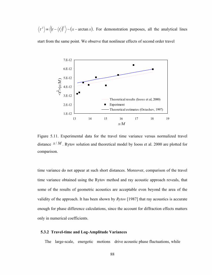
( ) ( xxtt arctan~22 −−≡τ ) . For demonstration purposes, all the analytical lines
start from the same point. We observe that nonlinear effects of second order travel
1.E-12
2.E-12
3.E-12
4.E-12
5.E-12
6.E-12
7.E-12
13 14 15 16 17 18 19x/M
<t>(
x/M
)
Theoretical results (Iooss et al, 2000)ExperimentTheoretical estimates (Ostashev, 1997)
Figure 5.11. Experimental data for the travel time variance versus normalized travel
distance /x M . Rytov solution and theoretical model by Iooss et al. 2000 are plotted for
comparison.
time variance do not appear at such short distances. Moreover, comparison of the travel
time variance obtained using the Rytov method and ray acoustic approach reveals, that
some of the results of geometric acoustics are acceptable even beyond the area of the
validity of the approach. It has been shown by Rytov [1987] that ray acoustics is accurate
enough for phase difference calculations, since the account for diffraction effects matters
only in numerical coefficients.
5.3.2 Travel-time and Log-Amplitude Variances
The large-scale, energetic motions drive acoustic phase fluctuations, while
88

3.0E-04
5.0E-04
7.0E-04
9.0E-04
1.1E-03
1.3E-03
1.5E-03
0.32 0.34 0.36 0.38 0.4 0.42 0.44 0.46x (m)
<2 >
Experiment Gaussian spectrum, D~1Kolmogorov spectrum Gaussian spectrum, D>>1
Figure 5.12. Experimental data for the log-amplitude variance as a function of travel
distance. Rytov solution for Kolmogorov spectra, Gaussian spectra and Frauhofer
diffraction are plotted for comparison.
smaller-scale motions drive the amplitude fluctuations [Wilson, 2000]. The energy-
containing subrange play the primary role in the experiment reported here. For our
experimental conditions the smallest, Kolmogorov, scale is l , while the
largest, integral scale has a size of the grid spacing,
m40 106.5 −⋅≈
m0 0.025L = . The diffraction region
is approximately defined as , so that according to the geometry of the
experiment our experimental domain falls into the diffraction region. Figure 5.12 shows
experimental data for log-amplitude variations plotted along with theoretical results,
Equation (3.108), derived in Chapter 3.7 for Kolmogorov spectra, Gaussian spectra and
its limiting case, Frauhofer diffraction for
λλ // 20
20 LLl <<
D >> 1
89
22 22 2
20
4arctan arctan1 18
vk lx D DD Dε c
σπχ σ = − + −
, ( )24 /D x kl= ( 5.8)
In case of D close to 1, which is the case in our experiment, the non-linearity due to
arctangent is well established. The general form of the log-amplitude variance in the case
of Gaussian spectra, which takes into consideration small diffraction effects, is the best fit
for our data. For demonstration purposes, all the analytical lines start from the same
point.
5.4 Methodology for Determination of Statistical Characteristics of Grid Generated
Turbulence
Experimental data were obtained for ultrasonic wave propagation downstream of a
non-heated and heated grid in a wind tunnel for different angular orientations of the
acoustic waves with respect to the mean flow. Since travel time fluctuations contain
information about the turbulence the developed methodology suggests using statistics of
travel time fluctuations for recovering of the correlation functions and spectra of
turbulent velocity and sound speed fluctuations [Andreeva and Durgin, 2001, 2002,2003
(c)].
5.4.1 Methodology for Determination of Correlation Functions of Velocity and
Acoustic Waves Fluctuations
The velocity and temperature fluctuations were generated simultaneously using a
heated grid. Nine cases of different distances L for two different temperatures
and , are studied. The defined temperatures correspond to the T 59 F= o T 159 F= o
90
temperature of aluminum rods of the grid. The angle β in Figure 5.1 is changed from 0
to 40 degrees with 5-degree step. It was experimentally demonstrated that for an open
loop tunnel thermal stratification is not significant even for low-speed flows, and also that
the mean air temperature is independent of downstream location within the range
considered [Yeh and van Atta, 1973; Sepri, 1976]. In the earlier works [Yeh and van Atta,
1973; Sepri, 1976] it was found that near the grid the wall temperature is higher than that
of the fluid because of the radiation from the hot grid. Therefore, the measurements were
collected at , where radiation effects are negligible. "45 "25/ ÷=Mx
M
Pr R
( )'
'40 0
1 , 's s
t K x xc
= ∫ ∫
The mean flow velocity was 5.3=U m/s. During the recording of turbulent data the
low velocity was chosen in favor of higher velocity in order to maximize the effect of
temperature fluctuations. The Reynolds number based on Re M and U was about
6000 and the corresponding Péclet number e ~ 4350M MPe = ; for the
working fluid air. Following the strategy described in the Section 3.6 we first use
flowmeter integral equation for the case of temperature of ,
Pr = 0.725
59 Fo
( )59 , 'FuK s s dxdx ' . ( 5.9)
In many practical problems, the form of the correlation function is not known.
However, its general shape is often approximated by a Gaussian function. It is very
convenient for analytical studies of wave propagation in random media, and, besides, it
allows taking into consideration the effect of the largest inhomogeneities in a medium on
the statistical moments of a sound field [Ostashev, 1997]. In addition, the combination of
numerical simulations and analytical approximations confirmed that a sound pulse tend to
91
effectively obey Gaussian statistics [Dacol, 2001]. We represent the correlation function
in equation (5.9) by
( ) ( )( ) ( )259 2 2 2 2 2
59 59, ' exp ' / exp /F
t t tF FK s s s s l lσ σ= − − = −τ . ( 5.10)
Here 2tσ is a variance of travel time fluctuations. Selection of l is problematic. In some
applications is chosen to be equivalent to a Taylor microscale. A better procedure is to
choose on the basis of the integral length scale of the turbulence [Ostashev, 1997].
Since we are considering travel time fluctuations in, rigorously speaking, diffractive
media in the approximation of ray acoustics, we should realize that there is some
uncertainty up to some numerical coefficient [Rytov et al, 1978]. Figure 5.13
demonstrates correlation function of travel time obtained using experimental data as a
function of separation distance compared with Gaussian curve providing the best fit. The
experimental data allow us to determine the unknown coefficients, and
. Integration of equation (5.10) with known
l
l
0.0036
2 9.85 15t eσ = −
2l = 2tσ and leads to the following
form of correlation function of turbulent velocity
2l
( ) ( ) (2 2
59 4 2 2 4 2 2 259 59' 2 42 exp / 4 exp /t tF F F
uK c l cl l
σ στ τ τ
= − − −
o o o )lτ
. ( 5.11)
It is apparent that the correlation function of turbulent velocity is no longer Gaussian,
although a Gaussian part is present in the first term in equation (5.11) and the second
term vanishes rapidly with distance. Figure 5.14 shows the correlation function of
turbulent velocity for our particular experimental data. The variance of velocity
fluctuations is 2
2 4' 22 0.0801t
u clσσ = = . At the same time we know, that
0.52'u uσ ′= ,
92
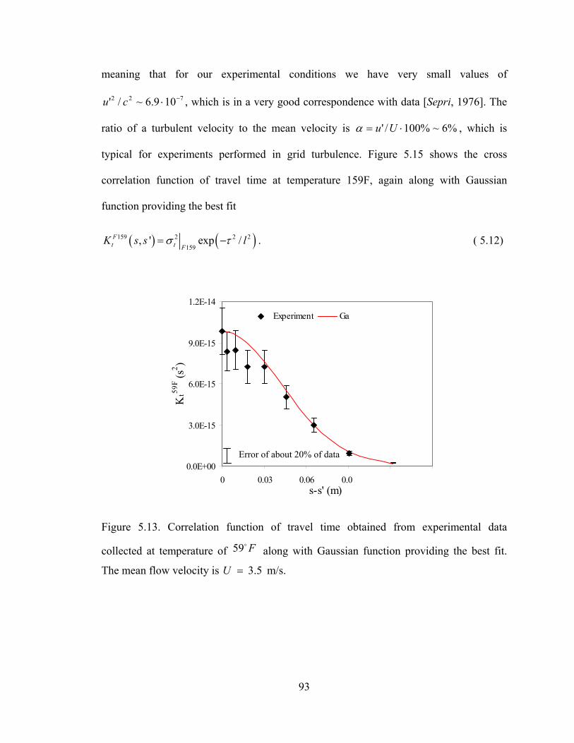
meaning that for our experimental conditions we have very small values of
, which is in a very good correspondence with data [Sepri, 1976]. The
ratio of a turbulent velocity to the mean velocity is
722 109.6~/' −⋅cu
%6~%100/' ⋅= Uuα , which is
typical for experiments performed in grid turbulence. Figure 5.15 shows the cross
correlation function of travel time at temperature 159F, again along with Gaussian
function providing the best fit
( )159 2, 'Ft t F
K s s
9 0.12 0.15
ussian Function
( 2 2
159exp / lσ τ= − . ( 5.12) )
0.0E+00
3.0E-15
6.0E-15
9.0E-15
1.2E-14
s-s' (m)
Kt59
F (s2 )
Experiment Ga
0 0.03 0.06 0.0
Error of about 20% of data
Figure 5.13. Correlation function of travel time obtained from experimental data
collected at temperature of 59 along with Gaussian function providing the best fit.
The mean flow velocity is
Fo
5.3=U m/s.
93

-3E-12
-2E-12
-1E-12
0
1E-12
2E-12
3E-12
4E-12
5E-12
6E-12
0 0.03 0.06 0.09 0.12 0.15
s-s' (m)
[Ku'
(m2 /s2 )]/
c4
Figure 5.14. Experimentally obtained correlation function of turbulent velocity.
0
5E-14
1E-13
1.5E-13
2E-13
2.5E-13
0 0.03 0.06 0.09 0.12 0.15
s-s' (m)
Kt15
9F (s
2 )
Experiment Gaussian Function
Figure 5.15. Correlation function of travel time obtained from experimental data
collected at temperature of 159 along with Gaussian function providing the best fit.
The mean flow velocity is
Fo
5.3=U m/s.
94
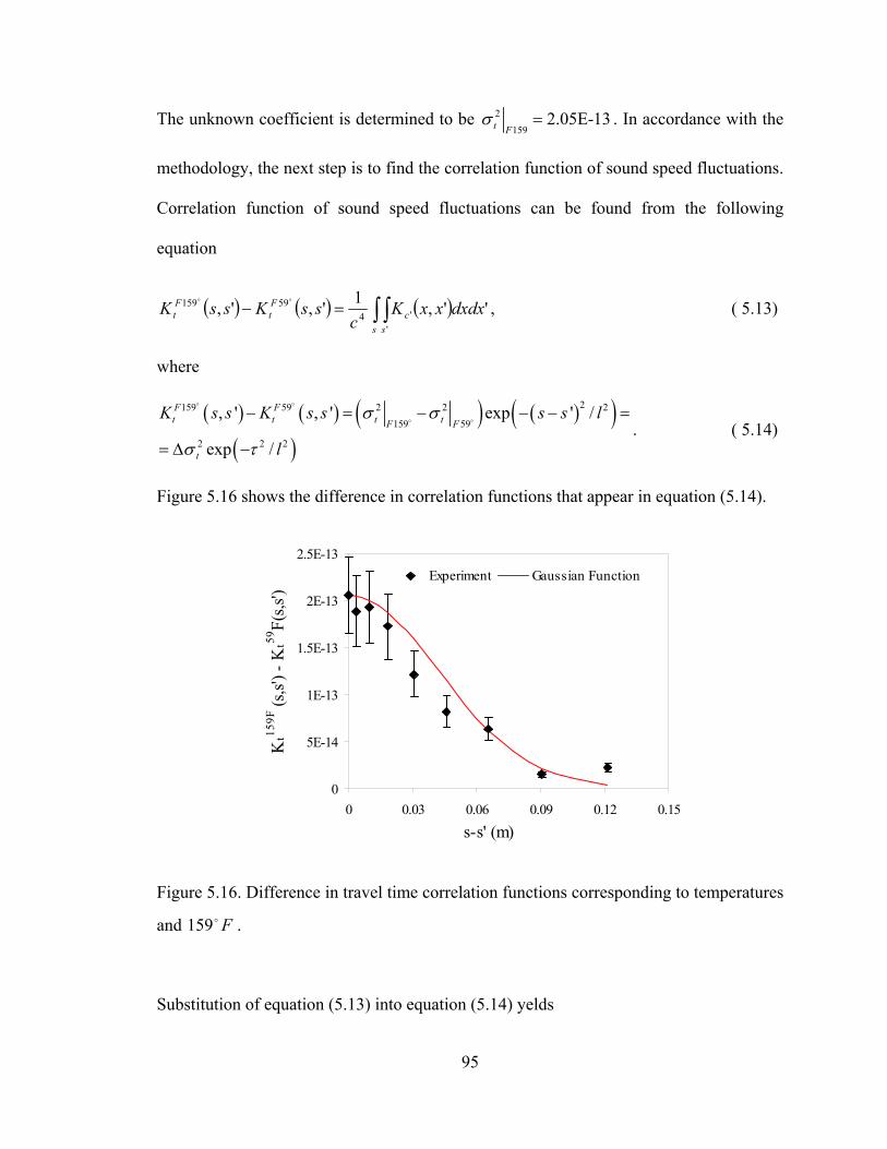
The unknown coefficient is determined to be 2
1592.05E-13t F
σ = . In accordance with the
methodology, the next step is to find the correlation function of sound speed fluctuations.
Correlation function of sound speed fluctuations can be found from the following
equation
( ) ( ) ( )∫ ∫=−s s
cFt
Ft dxdxxxK
cssKssK
''4
59159 ',1',',oo
' , ( 5.13)
where
( ) ( ) ( ) ( )( )( )
2159 59 2 2 2
159 59
2 2 2
, ' , ' exp ' /
exp /
F Ft t t tF F
t
K s s K s s s s l
l
σ σ
σ τ
− = − − −
= ∆ −
o o
o o=
. ( 5.14)
Figure 5.16 shows the difference in correlation functions that appear in equation (5.14).
0
5E-14
1E-13
1.5E-13
2E-13
2.5E-13
0 0.03 0.06 0.09 0.12 0.
s-s' (m)
Kt15
9F (s
,s') -
Kt59
F(s,s
')
15
Experiment Gaussian Function
Figure 5.16. Difference in travel time correlation functions corresponding to temperatures
and 159 . Fo
Substitution of equation (5.13) into equation (5.14) yelds
95
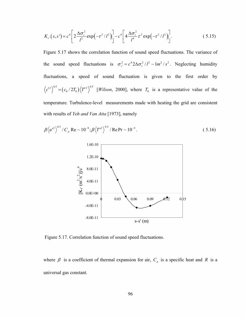
( ) ( ) (2 2
4 2 2 4 2' 2 4, ' 2 exp / 4 exp /t t
cK s s c l c ll lσ στ τ
∆ ∆= − − −
)2 2τ
2s
. ( 5.15)
Figure 5.17 shows the correlation function of sound speed fluctuations. The variance of
the sound speed fluctuations is . Neglecting humidity
fluctuations, a speed of sound fluctuation is given to the first order by
2 4 2 2 2' 2 / ~ 1 /c tc l mσ σ= ∆
( )0.5 0.520 0/ 2c c T T′ = 2′ [Wilson, 2000], where T is a representative value of the
temperature. Turbulence-level measurements made with heating the grid are consistent
with results of Yeh and Van Atta [1973], namely
0
55.0295.02 10~PrRe/';10~Re/' −− TCu p ββ . ( 5.16)
-8.0E-11
-4.0E-11
0.0E+00
4.0E-11
8.0E-11
1.2E-10
1.6E-10
0 0.03 0.06 0.09 0.12 0.15
s-s' (m)
[Kc'
(m2 /s2 )]/
c4
Figure 5.17. Correlation function of sound speed fluctuations.
where β is a coefficient of thermal expansion for air, C is a specific heat and p R is a
universal gas constant.
96
In the Table 5.1 we compare the basic flow parameters of the flow conditions such as
standard deviation of velocity fluctuations uσ , rate of dissipation uε , Kolmogorov length
scale , with corresponding wave number , time scale kl kk kτ , velocity scale , Taylor
microscale
kv
Tλ with corresponding Reynolds number Reλ , and Reynolds number based
on the mesh size M and mean velocity U. Standard deviation of turbulent velocity is
recovered from travel time measurements, consequently it is extremely important to
measure the length of a travel path precisely, otherwise small inconsistency in measuring
the travel distance results in considerable errors in determination other flow parameters.
Standard deviation of velocity fluctuations is almost three times as higher as it was
experimentally measured by Yeh and van Atta [1973]. Exceedingly high Reynolds
number is a consequence of a rough approximation of the standard deviation
of turbulent velocity.
4~ 00λR
5.4.2 Spectrum of Grid-Generated Turbulent Flow.
Early works on wave propagation in random media were based on 3-D Gaussian
turbulence models [Wilson, 2000]. As it was mentioned above, the model has an
advantage of analytical convenience. However, one range of turbulence structure it does
not capture is the inertial subrange, where energy is proportional to the wave number
raised to the power, which exists in high Reynolds number flows, such as
atmosphere [Wilson, 2000]. For the present experimental conditions an inertial subrange
is not expected in the power spectrum. Under similar conditions Van Atta and Chen
[1968] reported the absence of an inertial subrange in their velocity spectra for unheated
grids. Yeh and Van Atta [1973], Sepri [1976] observed no inertial subrange in the velocity
5 / 3−
97
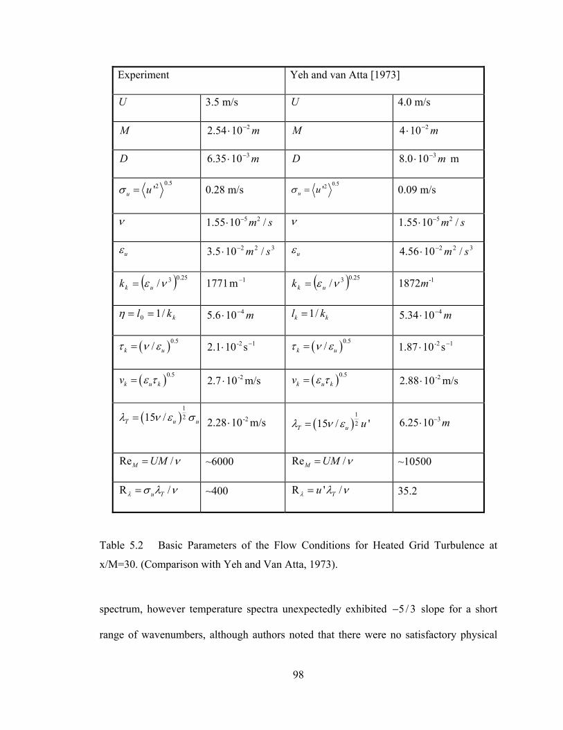
Experiment Yeh and van Atta [1973]
U 3.5 m/s U 4.0 m/s
M m21054.2 −⋅ M m2104 −⋅
D m31035.6 −⋅ D m3100.8 −⋅ m
0.52'u uσ = 0.28 m/s 0.52'u uσ = 0.09 m/s
ν 5 21.55 10 /m s−⋅ ν 5 21.55 10 /m s−⋅
uε 322 /105.3 sm−⋅ uε 322 /1056.4 sm−⋅
( ) 25.03/νε ukk = 1m 1771 − ( ) 25.03/νε ukk = -11872m
kkl /10 ==η m4106.5 −⋅ 1/k kl k= m41034.5 −⋅
( )0.5/k uτ ν ε= 1-2 s102.1 −⋅ ( )0.5/k uτ ν ε= 1-2 s101.87 −⋅
( )0.5k u kv ε τ= m/s102.7 -2⋅ ( )0.5
k u kv ε τ= m/s102.88 -2⋅
( )1215 /T u uλ ν ε σ=
m/s102.28 -2⋅ ( )
1215 / 'T u uλ ν ε= 36.25 10 m−⋅
Re /M UM ν= ~6000 Re /M UM ν= ~10500
R u Tλ /σ λ ν= ~400 R ' /Tuλ λ ν= 35.2
Table 5.2 Basic Parameters of the Flow Conditions for Heated Grid Turbulence at
x/M=30. (Comparison with Yeh and Van Atta, 1973).
spectrum, however temperature spectra unexpectedly exhibited 5 / 3− slope for a short
range of wavenumbers, although authors noted that there were no satisfactory physical
98

explanation for the appearance of the temperature spectrum.
The one-dimensional energy spectra were directly calculated from analytical
expressions of cross-correlation function of turbulent velocity and sound speed
fluctuations.
( ) ( )∫∫+∞+∞
∞−
=−=Φ0
)cos(1)exp(21 τττ
πτττ
πdkKdikK ttt . (5.17)
The PSD of the travel time at the room temperature is
( AakaARTt /exp
21 2−=Φ ππ
). ( 5.18)
The PSD of the turbulent velocity is
( ) ( )
( ) ( )
242 259
'0
242 2 259
40
( ) exp / cos
exp / cos
t Fu
t F
ck la
c l k dl
σk dτ τ τ
π
στ τ τ τ
π
+∞
+∞
Φ = −
− −
∫
∫
o
o
−
. (5.19)
Integration of Equation (5.16) yields to the final expression for the PSD of turbulent
velocity
( )4 2 2
2 2 2' 259
1( ) exp / 424u t F
c k kl k ll
ω σπ
Φ = − +
o . ( 5.20)
As expected, the PSD of sound speed fluctuations will have the same form, the only
difference will be in the numerical coefficient, 2tσ∆ instead of 2
59t Fσ
o. Figure 5.18
shows typical spectra for turbulent velocity and sound speed fluctuations. It is remarkable
that the spectral shapes appear unchanged at each of the locations, but that they appear to
be shifted uniformly in magnitude. The appearance of such difference was observed in
experiments by Sepri [1971, 1976], who studied velocity and temperature spectra under
99
similar conditions. In Figure 5.19 we compare 1-D velocity spectra is compared with one
obtained experimentally by Yeh and van Atta. Experiments by Yeh and van Atta were
carried out in the 0.76m x 0.76m 9m test section of the low turbulence wind tunnel. The
grid mesh size was M was 0.04m, with tubular rods of diameter of 0.008m. Comparison
reveals good correspondence between the velocity spectra recovered from travel time
measurements and the one, measured experimentally for the wave number up to
. For the larger wave numbers the present velocity spectra is different from
the measured velocity spectra. There are several aspects that may explain this difference.
First, our velocity spectra are recovered from experimental data for travel time, modeled
by the Gaussian function. Apriori, we did not expect to observe -5/3 slope corresponding
to the inertial subrange exhibited by the velocity spectra data by Yeh and van Atta [1973].
Secondly, due to the fact that turbulent velocity spectra as well as the sound speed
fluctuations spectra were drawn directly from travel time data, uncertainty in
determination of a length of the travel path leads to considerable errors in modeling of the
velocity spectra.
1100k m−=
100
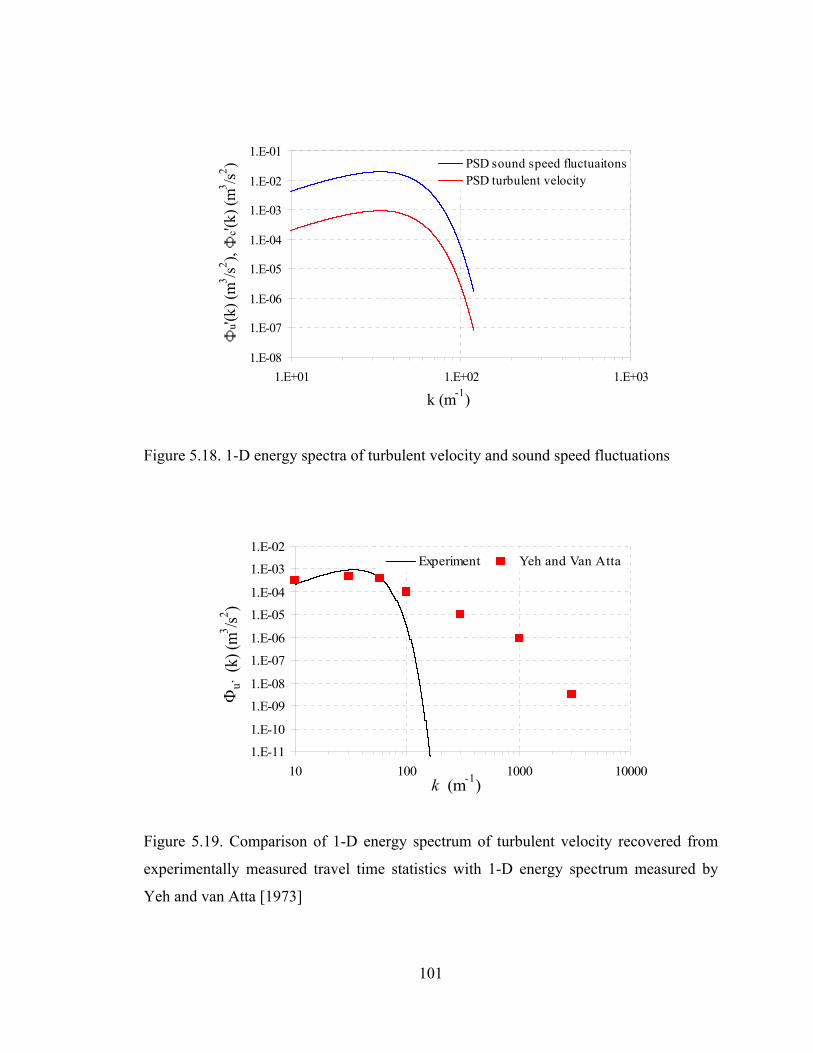
1.E-08
1.E-07
1.E-06
1.E-05
1.E-04
1.E-03
1.E-02
1.E-01
1.E+01 1.E+02 1.E+03
k (m-1)
u'(k)
(m3 /s2 ),
c'(k)
(m3 /s2 ) PSD sound speed fluctuaitons
PSD turbulent velocity
Figure 5.18. 1-D energy spectra of turbulent velocity and sound speed fluctuations
1.E-11
1.E-10
1.E-09
1.E-08
1.E-07
1.E-06
1.E-05
1.E-04
1.E-03
1.E-02
10 100 1000 10000k (m-1)
u'(k)
(m3 /s2 )
Experiment Yeh and Van Atta
Φu ’
Figure 5.19. Comparison of 1-D energy spectrum of turbulent velocity recovered from
experimentally measured travel time statistics with 1-D energy spectrum measured by
Yeh and van Atta [1973]
101
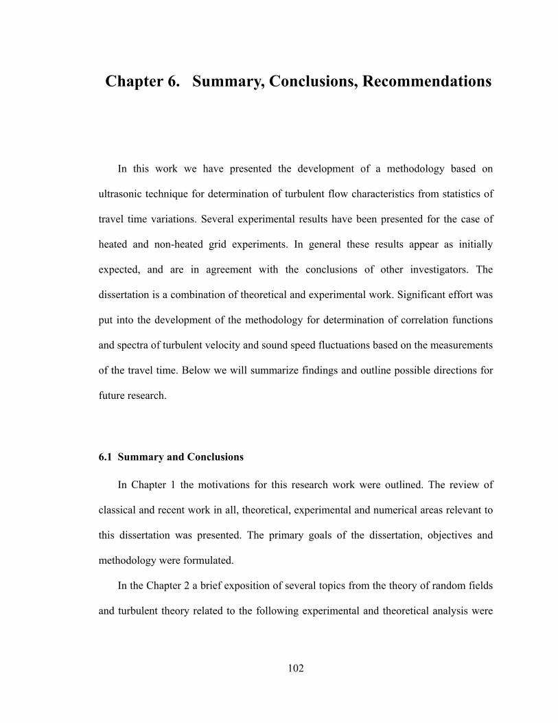
Chapter 6. Summary, Conclusions, Recommendations
In this work we have presented the development of a methodology based on
ultrasonic technique for determination of turbulent flow characteristics from statistics of
travel time variations. Several experimental results have been presented for the case of
heated and non-heated grid experiments. In general these results appear as initially
expected, and are in agreement with the conclusions of other investigators. The
dissertation is a combination of theoretical and experimental work. Significant effort was
put into the development of the methodology for determination of correlation functions
and spectra of turbulent velocity and sound speed fluctuations based on the measurements
of the travel time. Below we will summarize findings and outline possible directions for
future research.
6.1 Summary and Conclusions
In Chapter 1 the motivations for this research work were outlined. The review of
classical and recent work in all, theoretical, experimental and numerical areas relevant to
this dissertation was presented. The primary goals of the dissertation, objectives and
methodology were formulated.
In the Chapter 2 a brief exposition of several topics from the theory of random fields
and turbulent theory related to the following experimental and theoretical analysis were
102

given.
Theoretical model
Chapter 3 was devoted to the derivation and analysis of the equations describing the
propagation of acoustical waves in inhomogeneous moving media. Two well known
approximate theories of wave propagation, namely ray acoustics and the Rytov method
were presented. Statistical moments of a sound field were calculated using these two
approaches following the reviews of published works. The theory of travel time
fluctuations of sound waves due to the turbulence in the atmosphere based on the
Kolmogorov’s “2/3” law was presented and the physical and mathematical issues related
to the basic flowmeter equation were addressed. Special attention was put into the
reformulation of the classical flowmeter equation in the form that includes turbulent
velocity and sound speed fluctuations. The resulting integral equation in terms of
correlation functions for the travel time, turbulent velocity and sound speed fluctuations
is novel and important not only in the perspective of development of the methodology for
spectral analysis of isotropic homogeneous turbulence but also as an important issue in
achieving of a higher accuracy of ultrasonic devices.
Experimental model
The ultrasonic technique was employed for diagnostics and determination of the
statistics of grid-generated turbulence. Chapter 4 was devoted to the description of the
experimental apparatus. The major steps of the performance of ultrasonic measurement
system with a discussion of each component of the system, namely, ultrasonic flowmeter,
Data Acquisition Cards, LabVIEW software and characteristics of each component were
summarized in this chapter.
103
Chapter 5 was devoted to the key aspect of the dissertation: application of the travel-
time ultrasonic technique for data acquisition in the grid-generated turbulence and
analysis of the experimental data. The difficulty of obtaining laboratory measurements of
phase or time of flight variance, as well as amplitude variance is indicated by the dearth
of data. The chapter was opened with an overview of ultrasonic technique. The effect of
turbulence on acoustic waves in terms of the travel time was studied for various mean
velocities and for different angular orientations of the acoustic waves with respect to the
mean flow. The overview was followed by the analysis of the effects that turbulence has
on acoustic signals developed in the context of ray acoustic approach. Further, the
situation when mathematical conditions for ray acoustics are violated and ray acoustic
approach is no longer valid was discussed. Rytov’s approach was used to study the
influence of turbulence in terms of second moments of the travel time and log-amplitude
fluctuations. Comparison with theoretical results provided in literature was performed. In
the second half of Chapter 5 experimental data were obtained for ultrasonic wave
propagation downstream of a heated and non-heated grid for different angular
orientations of the acoustic waves with respect to the mean flow. A new methodology for
determination of correlation functions and spectra of turbulent velocity and sound speed
fluctuations has been proposed. The travel time statistics are approximated by a Gaussian
function. The coefficients and decay exponent of Gaussian function are determined by
the experimental data. Originally meant for ideal flow ultrasonic flowmeter equation has
been reformulated in terms of correlation functionsin order to account for turbulent
velocity and sound speed fluctuations.
.
104
1. It has been experimentally demonstrated that an ultrasonic travel-time method can be
efficiently utilized for determination of turbulent flow statistical characteristics in
laboratory conditions.
2. Simple methodology using the ultrasonic technique together with Kolmogorov’s 2/3
law was implemented for diagnostic of the grid-generated turbulent flow.
a. Methodology was validated using analytical estimates obtained from ray acoustic
theory.
b. In the experiment with different values of mean velocity, the experimental results
have indicated that there is strong dependence on the former.
c. The experimental results have shown that the ultrasonic method along with ray
acoustic approach can be efficiently utilized for measuring characteristics of
turbulent flow in laboratory scale, such as structure coefficient, C (m2/3/s).
3. From the travel time measurements performed in both turbulent and non-turbulent
media, Fermat’s principle is demonstrated.
4. Using experimental data of travel time effect of turbulence on acoustic wave
propagation has been demonstrated in terms of travel time variation and log-
amplitude variation. The experimental data have been interpreted using the ray
acoustic method and diffraction theory, or Rytov’s method.
a. It is clear from experimental results for travel time variance that in the presence of
small diffraction effects, the ray acoustic approach is valid, so area of ray acoustic
105
approach is broader than the rigorous sufficient conditions defined, at least for
travel-time fluctuations.
b. The experimental data confirm the Rytov theory in that amplitude variation is
greatly influenced by diffraction effects.
5. Experimental data for the case of both, velocity and thermal turbulence interpreted
using updated version of flowmeter equation, reveal a significant effect due to sound
speed fluctuations, thus, sound speed fluctuations may not be neglected in the
flowmeter equation as has often been supposed previously both in experiments and
theory.
6. The results provided by the methodology appear to be consistent with the wealth of
experimental data provided.
7. Updated flowmeter technology has a great potential for flow metering in industrial
facilities for various flow types, including non-ideal flows, thus reducing errors
caused by disturbances of the flow profile.
8. The combination of the proposed methodology together with ultrasonic technique
benefits not only from high accuracy provided by high-tech equipment, but also
offers a portable, simple in installation and use apparatus that can be used for
turbulent flow diagnostic in commercial and non-commercial applications.
106
6.2 Recommendations
1. The experimental data presented as well as their interpretation, are a subject to re-
examination in improved experimental conditions. Namely,
• Well-controlled mean temperature
• Stable wind tunnel flow at low speeds
• Extremely accurate determination and control of a travel distance
• Accurate determination of the temperature far downstream the grid, since small errors
in temperature determination may lead to large errors in sound speed fluctuations
2. In situ characterization of the turbulence as well as a good source of data for a
comparison ultrasonic measurements could be combined probe studies (hot, cold wire
anemometry).
3. Along theoretical lines it would be useful to examine the von Karman spectrum for
travel time experimental data approximation since the von Karman in many case,
especially in a grid-generated turbulent flow it provides a fairly good approximation
to the spectrum of turbulence [Ostashev, 1997; Wilson, 2000].
4. The methodology developed based on the measurements of the travel time
fluctuations at the receiver can be used to reconstruct not only velocity but also
temperature field.
5. The basic theory of wave propagation in turbulent media demonstrates the linear
107
increase of travel-time variance with the propagation distance [Chernov, 1960].
However, recent numerical and theoretical studies exhibit an almost quadratic growth
of travel time variance with travel distance [Karweit et al, 1991; Iooss et al, 2001].
The reason for this behavior is not entirely understood yet, but it proved to be closely
related to the occurrence of first caustics [Kulkarny and White, 1982; Blanc-Benon et
al, 1991, Klyatskin, 1993]. It would be useful to perform similar experiments for
larger travel distances in order to detect nonlinear behavior of travel time variance
[Durgin, et al., 2004 (accepted)].
108
Bibliography
Andreeva, T.A., Durgin, W.W., Weber, F.J., Johari, H, “Determination of Statistical Characteristics of Isotropic Turbulence,” Proceedings of ASME FEDSM’01, ASME Fluids Engineering Division Summer Meeting, New Orleans, Louisiana, May 29-June 1, 2001.
Andreeva T.A and Durgin, “Ultrasonic Technique in Characterization of the Grid-Generated Turbulent Flow,” Advanced Problems in Mechanics, XXX International Conference, Russia, St.-Petersburg, June 22-July 2, 2002.
Andreeva T.A. and Durgin, W.W., “Ultrasonic Technique for Investigation of the Effect of Grid-generated Turbulence on Sound Wave Propagation, “AIAA Paper 2003-1090, 41st Aerospace Science Meeting and Exhibit, Reno, Nevada, 2003 (a).
Andreeva T.A. and Durgin, W.W., “Ultrasound Technique for Prediction of Statistical Characteristics of Grid-Generated Turbulence,” AIAA Journal, Vol. 41(8), 2003, pp.1438-1443 (b).
Andreeva T.A. and Durgin, “Some Theoretical and Experimental Aspects in Ultrasonic Travel Time Method for Diagnostic of Grid-generated Turbulence,” World Congress on Ultrasonics , Paris, France, September 7-10, 2003 (c).
Andreeva, T.A, and Durgin, W.W., “Experimental Investigation of Ultrasound Propagation in Turbulent, Diffractive Media,” The Journal of the Acoustical Society of America, accepted for publication, 2003 (d).
Bass, H.E., Bolen, L.N., Raspet, R., McBride, W. and Noble, J., “Acoustic propagation through a turbulent atmosphere: Experimental characterization,” Journal of Acoustical Society of America, Vol. 90 (96), 1991, pp.3307-3313.
Batchelor, G.K., The Theory of Homogeneous Turbulence, Cambridge University Press., 1953.
Bergman L., and Schaefer, C., Optics of Waves and Particles., Berlin ; New York : W. de Gruyter, 1999.
Bendat, J. S. and Piersol, A.G., Random data; analysis and measurement procedures, New York, Wiley-Interscience, 1971.
Blanc-Benon, Ph., Juvé, D. and Comte-Bellot, G., “Occurrence of caustics for high-frequency caustic waves propagating through turbulent field,” Theoretical and Computational Fluid Dynamics Vol. 2, 1991, pp. 271-278.
Blanc-Benon, Ph., Juvé, D. and Chevret, P., “On the influence of the turbulence modeling for atmospheric sound propagation,” Journal of Acoustical Society of America,
109
Vol. 98, 1995, p. 2924.
Blokhintzev, D., The Acoustics of an Inhomogeneous Moving Medium, 1953
Boyse, W.E., “Wave Propagation and the Inversion in Slightly Inhomogeneous Media,” Ph.D. Dissertation, Stanford University, 1986.
Boyse, W.E., and Keller, J.B., “Short Acoustic, Electromagentic, and Elastic Waves in Random Media,” Journal of Optical Society of America A, Vol. 12, 1994, pp. 380-389.
Brassier, P., Hosten.B., Vulovic, F., “High-frequency Transducers and Correlation Method to Enchance Ultrasonic Gas Flow Metering,” Flow Measurement and Instrumentation, Vol. 12, 2001, pp. 201-211.
Brown, E.H. and Hall, F.F., “Advances in atmospheric acoustics,” Rev. Geophys. Space Phys.16, 47-110 (1978).
Chernov, L.A. Wave Propagation in a Random Medium, McGraw-Hill Book Company, Inc, 1960.
Chevret, P., Blanc-Benon, Ph. and Juvé, D., “A numerical model for sound propagation through a turbulent atmosphere near the ground,” Journal of Acousitcal Society of America, Vol. 100(6), 1996, pp. 3587-3599.
Clifford, S.F. and Lataitis, R.J., “Turbulence Effects on Acoustic Wave Propagation over a Smooth Surface,” Journal of Acoustical Society of America, Vol. 73(5), 1983, pp. 1545-1550.
Comte-Bellot, G. and Corrsin, S., “Simple Eulerian Time Correlation of Full- and Narrow- Band Velocity Signals in Grid-Generated “Isotropic” Turbulence,” Journal of Fluid Mechanics, Vol. 48, 1971, pp. 273-336.
Corrsin, S., “Encyclopedia of Physics,” Vol. 8(2), 1963, p.568.
Daigle, G.A., J.E. Piercy, J.E. and Embleton, T.F., “Effect of atmopspheric turbulence on the interference of sound waves near a hard boundary,” Journal of Acousitcal Society of America, Vol. 64, 1978, pp. 622-630.
Daigle, G.A., Piercy, J.E. and Embleton, T.F. “Line-of-site propagation through atmospheric turbulence near the ground,” Journal of Acoustical Society of America, Vol. 74, 1983, pp.1505-1513.
Daigle, G.A., Embleton, T.F.W. and Piercy, J.E., “Propagation of sound in the presence of gradients and turbulence near the ground,” Journal of Acoustical Society of America, Vol. 79, 1986, pp. 613-627.
Dacol, D.K., “Pulse Propagation in Randomly Fluctuating Media,” Journal of Acoustical Society of America, Vol. 109 (6), 2001, pp.2581-2586.
110
Di Iorio, D.D. and Farmer, D.M., “Separation of current and sound speed in the effective refractive index for a turbulent environment using reciprocal acoustic transmission,” The Journal of the Acoustical Society of America, Vol. 103(1), 1981, pp. 321-329.
Di Iorio, D.D. and Farmer, D.M., “Two-Dimensional Angle of Arrival Fluctuations,” The Journal of the Acoustical Society of America, Vol. 100(2) (Part1), 1996, pp.814-824.
Durgin, W.W., Meleschi, S.B. and Andreeva, T.A., “Experimental Investigation of Statistical Moments of Travel Time in Grid-Generated Turbulence,” 42nd AIAA Aerospace Sciences Meeting and Exhibit, 5-8 January, 2004, Reno, Nevada. (Accepted)
Ewart, T.E. and Percival, D.B., “Forward Scattered Waves in Rnadom Media: The Probability Distribution of Intensity,” The Journal of the Acoustical Society of America, Vol. 80, 1986, pp.1745-1753.
Godin, O.A., “Wave Equation for Sound in a Medium with Slow Current,” Trans. Acad. Sci. USSR Earth Science, Vol. 293 (1), 1987, pp.63-67.
Ho, C.M. and Kovasznay, L.S.G., “Modulation of an acoustic wave by turbulent shear flow,” U.S. Air Force Office of Scient. Res., Interim Tech. Rep., F44-620-69-C-0023, 1974.
Högström, U, “Review of some basic characteristics of the atmospheric surface layer,” Boundary- Layer Meteorology, Vol. 78, 1996, pp. 215-246.
Iooss, B., Blanc-Benon, Ph. and Lhuillier, C., “Statistical moments of travel times at second order in isotropic and anisotropic random media,” Waves in Random Media Vol. 10, 2000, pp. 381-394.
Iooss, B. and Galli, A., “Statistical tomography for seismic reflection data,” Proceedings of the 6th International Geostatistics Congress, Cape Town, South Africa, April 2000.
Ishimaru, A., Wave Propagation and Scattering in Random Media, Academic, New York, 1978.
Johari, H. and Durgin, W.W., “Direct Measurements of Circulation using Ultrasound,” Experiments in Fluids, Vol. 25, 1998, pp.445-454.
Jojnson, M.A., Raspet, R. and Bobak, M.T., “A Turbulence Model for Sound Propagation from an Elevated Above Level Ground,” The Journal of the Acoustical Society of America, Vol.81(3), 1987, pp. 638-646.
Karweit, M., Blanc-Benon, Ph., Juvé, D. and Comte-Bellot, G., Simulation of the Propagation of an Acoustic Wave through a Turbulent Velocity Field: a Study of Phase Variance,” The Journal of the Acoustical Society of America, Vol. 89(1), 1991, pp. 52-62.
Kistler, A.L., O’Brien, V. and Corrsin, S., “Preliminary Measurements of Turbulence and Temperature Fluctuations Behind a Heated Grid,” N.A.S.A. RM 54D19, 1954.
111

Kits, A.H. van Heyningen, “Solid State Doppler Wind Sensor,” Abstracts, SBIR Topic No. N85-181, 1987
Klyatskin, V.I., “Caustics in Random Media,” Waves in Random Media, Vol. 3, 1993, pp. 93-100.
Kolmogorov, A., “The Local Structure of Turbulence in Incompressible Viscous Fluid for Very Large Reynolds Numbers, C.R. Akad. Sci. SSSR, Vol. 30, 1941, pp. 301-305.
Kolmogorov, A.N., “Energy Dissipation with Locally Isotropic Turbulence,” DAN SSSR, Vol. 32(1), 1941, p.19
Kolmogorov, A., “A Refinement of Previous Hypothesis Concerning the local Structure in a Viscous Incompressible Fluid in High Reynolds Number,” Journal of Fluid Mechanics, Vol. 13, 1963, p.82.
Krasil’nikov, V.A., “Propagation of Sound in a Turbulent Atmosphere,” Doklady Acadenii Nauk SSSR (in Russian), Vol. 47, 1945, pp.486-489.
Krasil’nikov, V.A. “Phase Fluctuations in Ultrasonic Waves During Propagation of Sound in the Atmosphere,” Doklady Academii Nauk SSR (in Russian), Vol. 88, 1953, pp. 657-660.
Krasil’nikov, V.A., Sound and Ultrasound Waves in Air, Water and Solid Bodies, Jerusalem, 1963.
Krasil’nikov, V.A., “The Effect of Refractive Index Fluctuations in the Atmosphere on Propagation of Ultrashort Radio Waves,” Izvestiya AN SSSR, Seria Geograficheskaya I Geofizicheskaya, vol. 13(1), 1949, p.33
Kristensen, L., Lenschow, D. H., Kirkegaard, P. and Courtney, M., ‘‘The spectral velocity tensor for homogeneous boundary-layer turbulence,’’ Boundary-Layer Meteorology. Vol. 47, 1989, pp. 149–193.
Kulkarny, V.A. and White, B.S., “Focusing of Waves in Turbulent Inhomogeneous Media,” Journal of Physics of Fluids, Vol. 25 (10), 1982, pp. 1779-1784.
Landau, L.D. and Lifshitz, E.M., Course of Theoretical Physics, Fluid Mechanics, Volume 6, 2nd edition, Institute of Physical Problems, USSR Academy of Science, Moscow.
Leontovich, M.A., Journal of Experimental Physics, Vol. 6, 1936, p.561. In Russian
Loitsianskii, L.G., “Some Basic Laws of Isotropic Turbulent Flow,” Cent. Aero. Hydrodyn. Inst. Moscow, Rept. 440. (Trans. NACA TM 1079.) 1939.
Lawrence, R.S. and Strohbehn, J.W., “A survey of clear-air propagation effects relevant to optical communications,” Proceedings IEEE, Vol. 58, 1970, pp. 1523-1545.
112
Lynnworth, L.C., “Ultrasonic Measurements for Process Control,” Academic Press, San Diego, CA, 1989.
Mann, J., “The spatial structure of neutral atmospheric surface layer turbulence,” Journal of Fluid Mechanics, Vol. 273, 1994, pp. 141–168.
Mills, R.R. and Kistler, A.L., O’Brien, V. and Corrsin, S., “Turbulence and Temperature Fluctuations Behind a Heated Grid,” N.A.S.A. Technical Note 4288, 1958.
Mohamed, M.S. and LaRue J.C., “The Decay Power Law in Grid-generated Turbulence,” Journal of Fluid Mechanics, Vol. 219, 1990, pp. 195-214.
Monin, A.S. and Yaglom, A. M., Statistical Fluid Mechanics, Cambridge, MA: MIT Press, 1981.
Mydlarskii, L. and Warhaft, Z., “Passive Scalar Statistics in High_Péclet-number Grid Turbulence,” Journal of Fluid Mechanics, Vol. 358, 1998, pp. 135-175.
Nelkin, M., “Universality and Scaling in Fully Developed Turbulence,” Advanced Physics, Vol. 43, 1991, pp.143-181.
Nghiem-Phu, L. and Tappert, F., “Parabolic Equation Modeling of the Effects of Ocean Currents on Sound Transmission and Reciprocity in the Time Domain,” Journal of Acoustical Society of America,” Vol. 78(2), 1985, pp. 642-648.
Noble, J. M., Bass, H. E. and Raspet, R., “The Effect of Large-scale Atmospheric Inhomogeneities on Acoustic Aropagation,” Journal of Acoustical Society of America, Vol. 92, 1992, pp.1040–1046.
Obukhov, A.M., “Scattering of Sound in Turbulent Flow,” DAN SSSR, Vol. 30(7), 1941, pp. 611
Obukhov, A.M., “Characteristics of wind microstructures in the atmosphere near the surface,” Izv. Acad. Sci. USSR Atmos. Ocean. Phys., Vol. 3, 1951, p.49.
Obukhov, A.M., “ Energy Distribution in the Spectrum of Turbulent Flow,” Izvestiya AN SSSR, Seriya Geograficheskaya I Geofizichaskaya, Vol. 5(4/5), 1941, pp.453.
Ostashev, V.E. Acoustics in Moving Inhomogeneous Media, E & FN SPON, London, UK, 1997.
Ostashev, V.E., Salomons, E.M., Clifford, S.F., Lataitis, R.J., Wilson, D.K., Blanc-Benon, Ph., Juvé, D., “Sound propagation in a turbulent atmosphere near the ground: A parabolic equation approach,” Journal of Acoustical Society of America, Vol. 109(5), 2001, pp. 1894-1906.
Ostashev, V.E. and G. H. Goedecke, ‘‘Interference of direct and ground reflected waves in a turbulent atmosphere,’’ Proceedings of the 8th International Symposium on Long
113
Range Sound Propagation, Penn State University,1998, pp. 313–325.
Peltier, L. J., Wyngaard, J. C., Khanna, S. and Brasseur, J. G., ‘‘Spectra in the unstable surface layer,’’ Journal of atmospheric Science, Vol. 53, 1996, pp. 49–61.
Pierce, A.D., Acoustics: An Introduction to Its Physical Principles and Applications, McGraw-Hill, New York, 1981.
Pierce, A.D., “Wave Equation for Sound in Fluids with Unsteady Inhomogeneous Flow,” The Journal of the Acoustical Society of America, Vol. 87(6), 1990, pp. 2292-2299.
Robertson, J.S., Siegmann, W.L. and Jacobson, M.J., “Current and Current Shear Effects in the Parabolic Approximation for Underwater Sound Channel,” Journal of Acoustical Society of America, Vol. 77(5), 1985, pp. 1768-1780.
Roth, S.D., Acoustic Propagation in the Surface Layer under Convectively Unstable Conditions, Ph.D. Dissertation in Acoustics, The Pennsylvania State University, University Park, Pennsylvania, 1983.
Roth, M., Müller, G. and Snieder, R., “Velocity Shift in Random Media,” Geophysical Journal Internationa, Vol 115, 1993, pp. 552-563.
Rytov, S.M., Kravcov, Yu.A., Tatarskii, V.I., Elements of Random Process Theory: Principles of Statistical Radiophysics, Springer-Verlag, Berlin, 1987, Vol. 4.
Samuelides, Y., “Velocity shift using the Rytov approximation,” Journal of Acoustical Society of America, Vol. 104, 1998, pp. 2596-2603.
Schmidt, D.W., “Acoustical Method for Fast Detection and Measurement of Vortices in Wind Tunnels,”ICIASF’75 Record”, pp.216-228.
Schmidt, D.W., Tilmann, P.M., “Experimental Study of Sound-wave Phase Fluctuations caused by Turbylant Wakes,” Journal of Acoustical Society of America, Vol. 47, 1970, pp.1310-1324.
Sepri, P., “Two-point Turbulence Measurements Downstream of a Heated Grid,” The Physics of Fluids, Vol. 19 (12), 1976, pp. 1876-1884.
Snieder, T., and Aldridge, D.F., “Perturbation Theory for Travel Times,” Journal of Acoustical Society of America, Vol. 98, 1995, pp. 1565-1569
Sreenivasan, K.R. and Antonia, R.A., “The phenomenology of Small-Scale Turbulence,” Annual Review of Fluid Mechanics, Vol. 29, 1997, pp. 435-472.
Sreenivasan, K.R., Tavoularis, S., Henry, R. and Corrsin, S., “Temperature Fluctuations and Scales in Grid-generated Turbulence,” Journal of Fluid Mechanics, Vol. 100(3), 1980, pp. 597-621.
114
Stratonovich, R.L., Selected Topics in the Theory of Fluctuations in Radio Engineering, Sovetskoe Radio, 1961.
Tatarskii, V.I., Wave Propagation in a Turbulent Medium, McGraw-Hill, New York, 1961.
Tatarski, V.I., The Effect of the Turbulent Atmosphere on Waves Propagation, Israel Program for Scientific Translation, Jerusalem, 1971.
Tatarskii, V.I., Wave Propagation in Turbulent Media, (Nauka, Moscow, 1967, in Russian).
Tennekes, H. and Lumley, J.L., First Course in Turbulence, The MIT Press, 1972.
M.S. Uberoi and S. Wallis, “Effect of Grid Geometry on Turbulence Decay, ”Journal of Physics of Fluids, Vol. 10, 1967, pp. 1216-1230.
Van W. Atta and Chen, W.Y., Journal of Fluid Mechanics, Vol. 34, 1968, p.497.
Warhaft, Z., “Passive Scalars in Turbulent Flows,” Annual Review of Fluid Mechanics, Vol. 32, 2000, pp. 203-240.
Warhaft, Z., and Lumley, J.L., “The Decay of Temperature Fluctuations and Heat Flux in Grid-Generated Turbulence,”Structure and Mechanism of Turbulence, Vol. 2, Lectures Notes in Physycs, Vol. 76, 1978(a).
Warhaft, Z., and Lumley, J.L., “An Experimental Study of the Decay of Temperature Fluctuations in Grid-generated Turbulence,” Journal of Fluid Mechanics, Vol. 88 (4), 1978 (b), pp.659-684.
Wielandt, E., “On the Validity of the Ray Approximation for Interpreting Delay Times,” in Seismic Tomography, edited by G. Nolet (Reidel, Dordrecht, 1987), pp.85-98.
Weber, F.J., Ultrasonic Circulation-meter for Determining the Magnitude of Circulation about a Rapidly Pitching Airfoil, Master Thesis, Worcester Polytechnic Institute, 1994.
Wilken, W., ‘‘Experimental study of the influence of varying atmospheric conditions on sound propagation close to the ground’’ Acustica, Vol. 62, 1986, pp. 55–65.
Wilson, D.K., Acoustic Tomographic Monitoring of the Atmospheric Boundary Layer, Ph.D. Dissertation, The Pennsylvania State University, 1992.
Wilson, D.K., Brasseur, J.G., Gilbert, K.E., “Acoustic scattering and the spectrum of atmospheric turbulence,” The Journal of the Acoustic Society of America, Vol. 105(1), 1999, pp.30-34.
Wilson, D. K., “A turbulence spectral model for sound propagation in the atmosphere that incorporates shear and buoyancy forcing,” Journal of Acoustical Society of America,
115
Vol. 108 (5), 2000, pp.2021-2038.
Wilson, D. K. and Thomson, D. W., ‘‘Acoustic propagation through anisotropic, surface-layer turbulence,’’ The Journal of the Acousitcal Society of America, Vol. 96, 1994, pp. 1080–1095.
Yeh, T.T. and van Atta, C.W., “Spectral Transfer of Scalar and Velocity Fields in Heated-grid Turbulence,” Journal of Fluid Mechanics, Vol. 58, 1973, pp. 233-261.
Yeh, T.T. and Espina, P.I., “Special Ultrasonic Flowmeters for In-situ Diagnosis of Swirl and Cross Flow,” Proceedings of ASME Fluids Engineering Division Summer Meeting, FEDSM 2001-18037, 2001.
Yeh, T.T. and Mattingly, G.E., “Ultrasonic Technology: Prospects for Improving Flow Measurements and Standards,” Proceedings of the 4th International Symposium on Fluid Flow Measurements, Denver, Co, NAFFMC 1999 and Proceedings FLOMEKO 2000.
Yeh, T.T. and Espina P.I., Osella, S.A., “An Intelligent Ultrasonic Flow Meter for Improved Flow Measurements and Flow Calibration Facility,” IEEE Instrumentation and Measurement technology Conference, Budapest, Hungary, May 21-23, 2001.
116
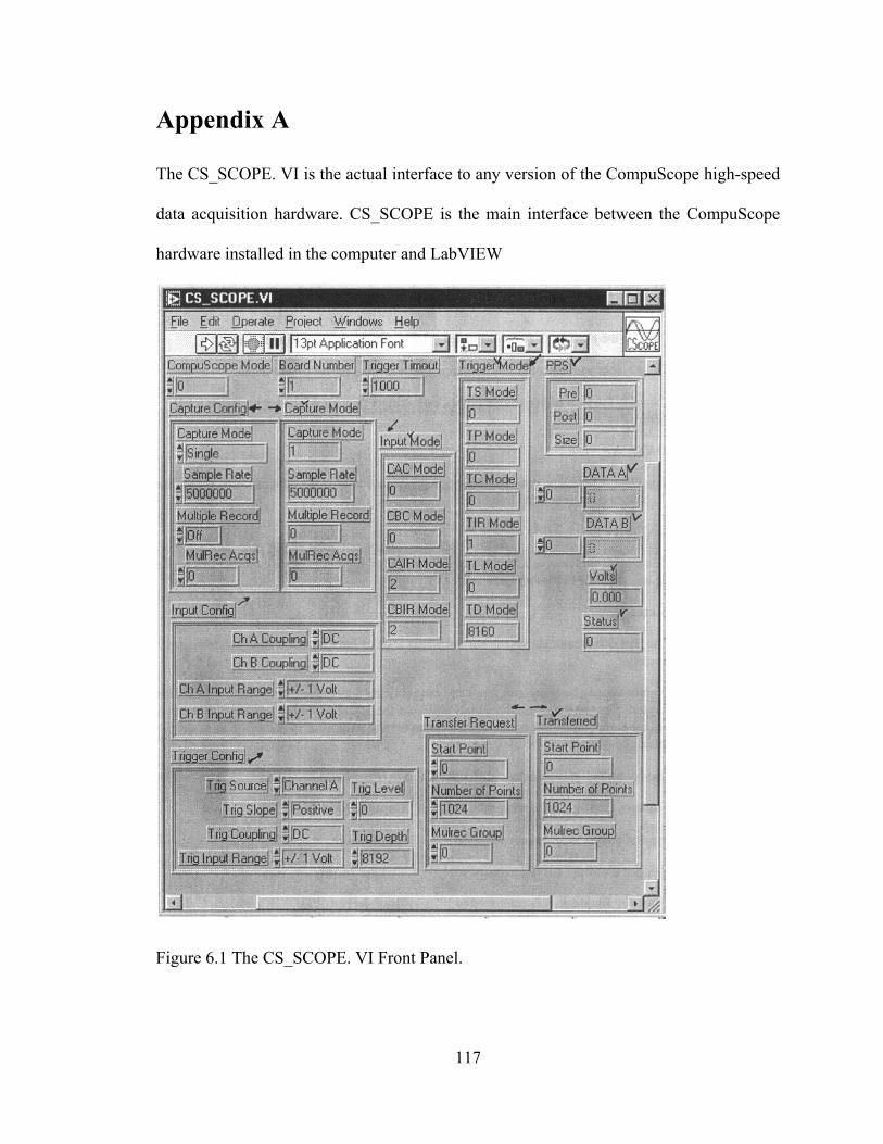
Appendix A
The CS_SCOPE. VI is the actual interface to any version of the CompuScope high-speed
data acquisition hardware. CS_SCOPE is the main interface between the CompuScope
hardware installed in the computer and LabVIEW
Figure 6.1 The CS_SCOPE. VI Front Panel.
117

The Gage Oscilloscope.VI is a program that uses the CompuScope modes to capture,
transfer and display data acquired from CompuScope board.
Figure 6.2. Gage Oscilloscope Sequence 0.
118

Figure 6.3. Gage Sample Oscilloscope. VI (demonstration mode).
119
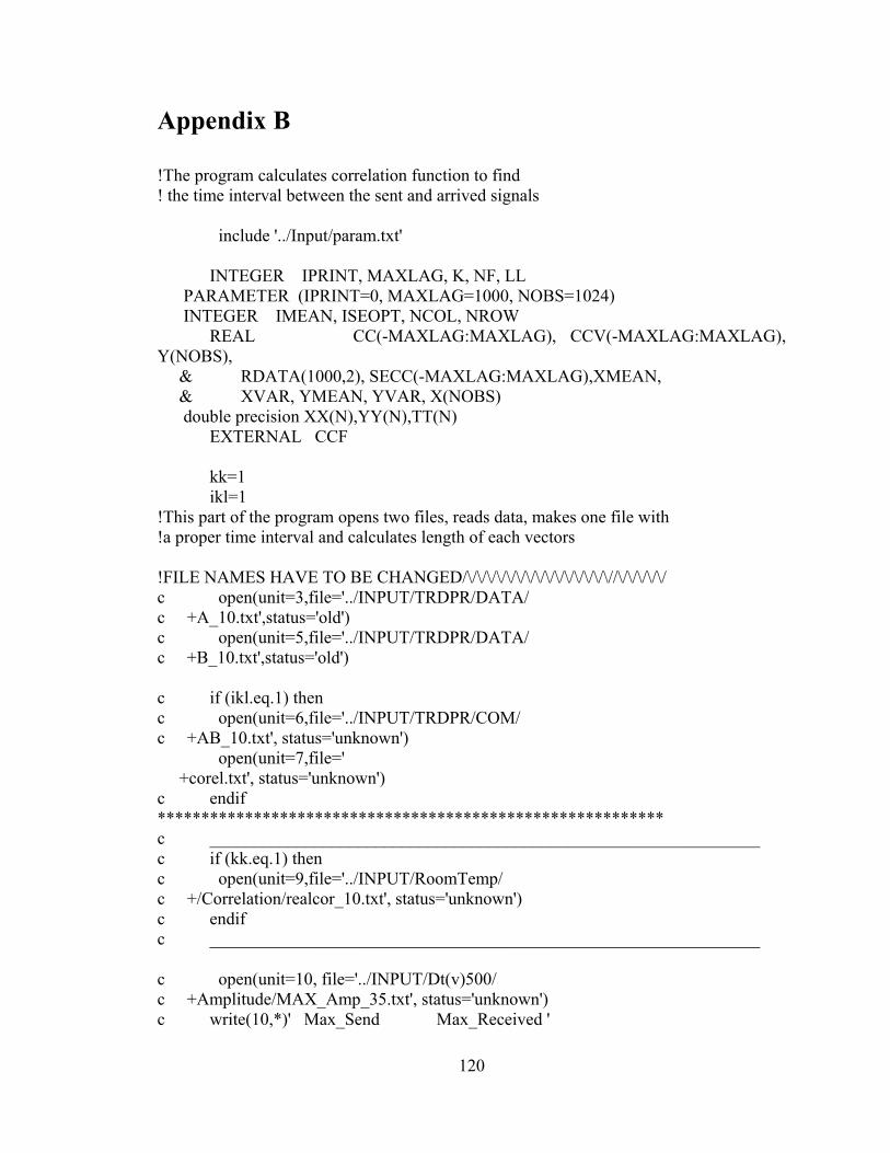
Appendix B
!The program calculates correlation function to find ! the time interval between the sent and arrived signals include '../Input/param.txt' INTEGER IPRINT, MAXLAG, K, NF, LL PARAMETER (IPRINT=0, MAXLAG=1000, NOBS=1024) INTEGER IMEAN, ISEOPT, NCOL, NROW REAL CC(-MAXLAG:MAXLAG), CCV(-MAXLAG:MAXLAG), Y(NOBS), & RDATA(1000,2), SECC(-MAXLAG:MAXLAG),XMEAN, & XVAR, YMEAN, YVAR, X(NOBS) double precision XX(N),YY(N),TT(N) EXTERNAL CCF kk=1 ikl=1 !This part of the program opens two files, reads data, makes one file with !a proper time interval and calculates length of each vectors !FILE NAMES HAVE TO BE CHANGED/\/\/\/\/\/\/\/\/\/\/\/\/\/\/\//\/\/\/\/\/ c open(unit=3,file='../INPUT/TRDPR/DATA/ c +A_10.txt',status='old') c open(unit=5,file='../INPUT/TRDPR/DATA/ c +B_10.txt',status='old') c if (ikl.eq.1) then c open(unit=6,file='../INPUT/TRDPR/COM/ c +AB_10.txt', status='unknown') open(unit=7,file=' +corel.txt', status='unknown') c endif ********************************************************** c _______________________________________________________________ c if (kk.eq.1) then c open(unit=9,file='../INPUT/RoomTemp/ c +/Correlation/realcor_10.txt', status='unknown') c endif c _______________________________________________________________ c open(unit=10, file='../INPUT/Dt(v)500/ c +Amplitude/MAX_Amp_35.txt', status='unknown') c write(10,*)' Max_Send Max_Received '
120
!THE LAST FILE IS THE ONE WITH PROPER TIME AND TWO COLUMNS OF DATA !/\/\/\/\/\/\/\/\/\/\/\/\/\/\/\/\/\/\/\/\/\/\/\/\/\/\/\/\/\/\/\/\/\/\ c do i=1,N c read(3,*,end=2) TT(i),YY(i) c end do c 2 continue c do i=1,N c read(5,*,end=4) TT(i),XX(i) c end do c 4 continue c do j=1,N c TT(j)=TT(2)*(j-1) ********************************** c print*,'TT=',TT(2),TT(j) c if (TT(2).GT.1.e-5) then c print*,'j=',j c endif ********************************** c if (ikl.eq.1) then c write(6,8)TT(j),XX(j),YY(j) c 8 format(3x,3(E15.6,3x)) c endif c enddo c close(3) c close(5) c close(6) !/\/\/\/\/\/\/\/\/\/\/\/\/\/\/\/\/\/\/\/\/\/\/\/\/\/\/\/\/\/\/\/\/\/\/ !/\/\/\/\/\/\/\/\/\/\/\/\/\/\/\/\/\/\/\/\/\/\/\/\/\/\/\\/\/\/\\/\/\/\/ PI = 4.*atan(1.) IMEAN = 1 ISEOPT = 0 !===================================================================== ! This block selects a data interval from all data c NF=N/NOBS c do LL=1,NF !====================================================================== c do J=NOBS*(LL-1)+1,LL*NOBS c X(-NOBS*(LL-1)+J)=1.*XX(J)
121
c Y(-NOBS*(LL-1)+J)=1.*YY(J) c end do CALL CCF (NOBS, X, Y, MAXLAG, IPRINT, ISEOPT, IMEAN, XMEAN, & YMEAN, XVAR, YVAR, CCV, CC, SECC) c S=0. print*,XMEAN, YMEAN do I=1,2*MAXLAG+1 c c if (CC(I).GE.S) then c S=CC(I) c K=I c endif c if (kk.eq.1) then write(7,*)(I-1)*0.1*PI,CC(I) c endif end do c write(7,*)'delta_T',K*TT(2) sum=0 do I=1,1024 sum=sum+Y(I) enddo averageY=sum/1024. smaxX=0. smaxY=0. do I=1, 1024 if (abs (X(I)).GT.smaxX) then smaxX=abs(X(I)) endif if (abs (Y(I)-averageY).GT.smaxY) then smaxY=abs(Y(I)-averageY) endif end do write (10,*)smaxX,smaxY c end do end Make sure your input files are in ../Input/*.* directory! !========================================================== open(unit=3,file='../INPUT/TRDPR/DATA/
122
123
+A_10.txt',status='old') open(unit=5,file='../INPUT/TRDPR/DATA/ +B_10.txt',status='old') open(unit=4,file='../INPUT/param.txt', status='unknown') i=1 1 read(3,*,end=10) t,t i=i+1 goto 1 10 N1=i j=1 2 read(5,*,end=20) t,t j=j+1 goto 2 20 N2=j if (N1.lt.N2) then N=N1 else N=N2 endif Print*,'N=',N write(4,5)N-1 5 format(' PARAMETER (N=',I8,')') write(*,*)'File "param.txt" has been successfully created' close(3) close(4) close(5) end