ultrasound technique for the dynamic mechanical analysis (dma) · ultrasound technique for the...
TRANSCRIPT
Ultrasound Technique for theDynamic Mechanical Analysis (DMA)of Polymers
M. Sc. Jarlath Mc Hugh
BAM-Dissertationsreihe • Band 31Berlin 2008
Impressum
Ultrasound Technique for theDynamic Mechanical Analysis (DMA)of Polymers
2008
Herausgeber:Bundesanstalt für Materialforschung und -prüfung (BAM)Unter den Eichen 8712205 BerlinTelefon: +49 30 8104-0Telefax: +49 30 8112029E-Mail: [email protected]: www.bam.de
Copyright © 2008 by Bundesanstalt fürMaterialforschung und -prüfung (BAM)
Layout: BAM-Arbeitsgruppe Z.64
ISSN 1613-4249ISBN 978-3-9812072-0-0
Die vorliegende Arbeit entstand an der Bundesanstalt für Materialforschung und -prüfung(BAM).
Ultrasound Technique for the Dynamic Mechanical Analysis (DMA) of Polymers
vorgelegt von B.Eng MSc Jarlath Mc Hugh
aus Longford, Irland
von der Fakultät III - Prozesswissenschaften der Technischen Universität Berlin
zur Erlangung des akademischen Grades
Doktor der Ingenieurwissenschaften - Dr.-Ing. -
genehmigte Dissertation
Promotionsausschuss:
Vorsitzender: Prof. Dr. rer. nat. H. J. Hoffmann Berichter: Prof. Dr.-Ing. M. H. Wagner Berichter: Dr. rer. nat. habil. W. Stark
Tag der wissenschaftlichen Aussprache: 24. Mai 2007
BERLIN 2007 D 83


To my Parents and Family - Thanks for your Support

Abstract
The objective of this work is to demonstrate the practical application and sensitivity of
ultrasound as a high frequency Dynamic Mechanical Analysis DMA technique for the
characterisation of polymers. Conventional DMA techniques are used to determine thermo-
mechanical behaviour of polymers by typically employing dynamic shear or tensile loading
modes at defined frequencies between 0.1 and 50 Hz. Sound waves may also be employed for
DMA applications and depending on type of wave propagated, shear G´, G´´ and longitudinal
L´, L´´ storage or loss modulus and tan(δ) may be determined from the measured acoustic
parameters sound velocity and amplitude. The primary advantage of ultrasound DMA is that
due to the compact sensor size it can easily be integrated into most manufacturing processes.
To demonstrate the sensitivity of ultrasound to variations in the viscoelastic properties
of polymers, the acoustic properties of a cured epoxy with an observed glass transition
temperature of 86 °C (tan(δ) peak, 1Hz) were monitored in a temperature range from 20 to
200 °C and compared to conventional DMA results. The influence of measurement frequency,
dispersion, hysteresis, reflections at material boundaries, and changes in material density on
the measured sound velocity and amplitude were taken into account. To support conclusions a
wide range of experimental data was evaluated using sensors operating in the frequency
ranges 400 to 800 kHz and 3 to 6 MHz. The ultrasound results are compared to the tensile
moduli E´, E´´ and tan(δ) measured using a conventional DMA technique operating at 0.1 to
33 Hz. Using different evaluation strategies such as the Williams Landel Ferry WLF equation
it was possible to study the sensitivity of wave propagation to variations in the viscoelastic
behaviour of a polymer. Taking advantage of this background knowledge, further
experimental results are presented with the aim of demonstrating the sensitivity of this
technique for cure monitoring applications and to the material transformations: gelation and
vitrification. For this purpose an epoxy resin was cured at a range of constant temperatures
whereby the curing reaction and the corresponding change in viscoelastic properties were
monitored. Analysis techniques employed included ultrasound at 3 to 6 MHz, Differential
Scanning Calorimeter DSC and Rheometry at 1 Hz. All results were summarised and
presented graphically. Additionally an Arrhenius relationship was employed enabling direct
comparison of results obtained from analysis techniques based on different working
principles. Using this information, it was possible to demonstrate the practical application and
the sensitivity of this technique to even small changes in viscoelastic properties of polymers.

Acknowledgements
I would like to thank my supervisor, Prof. Dr. Manfred W. Wagner at the Technical
University in Berlin for his supportive advice. In particular, I am very grateful to
Dr. habil. Wolfgang Stark for his motivational support and professional advice. Starting with
his supervision of my masters at Cranfield University, England he has always encouraged my
work. The time and effort he invested were voluntary and comes from his tremendous interest
and enthusiasm for this subject. I hope that in the future such commitment will obtain the
credit it deserves.
Further thanks to my colleagues at the BAM (Bundesanstalt für Materialforschung und
–prüfung) who supported me throughout my work. Thank you to Dr. Joachim Döring for
detailed and helpful discussions especially in the field of physical acoustics. Other colleagues
that have followed and supported this work from the beginning include Jürgen Bartusch who
helped program the FFT analysis software employed here and also Dr. Harald Goering who
aided in evaluating the results from the Differential Scanning Calorimeter. The support of my
superiors and in particular Dr. Anton Erhard and Dr. Werner Mielke for their aptness at
juggling contracts and designation of work which provided me with the freedom to
concentrate on this thesis is also gratefully acknowledged.
Last but not least, I would like to thank my family at home and abroad who supported
me throughout this work. You have been tremendous throughout and hopefully I have no
longer an excuse for forgetting all future birthdays and anniversaries – once again thank
you!!!!

xi
Contents
Notations and Abbreviations xv
1 Introduction 1
1.1 Objectives………………………………………………………………………….3
2 Characterisation of Elastic Properties of Polymers using Ultrasound 6 2.1 Literature Review and Background………………………………………………..6
2.1.1 Fundamental Development………………………………………………6
2.1.2 Characterisation of Polymers…………………………………………….8
2.1.3 Characterisation of Reactive Thermosetting Polymers…………………10
2.2 Wave Propagation and Dynamic Mechanical Analysis…………………………..12
2.2.1 Propagation of Waves…………………………………………………..12
2.2.2 Mechanical Oscillations and Wave Theory…………………………….13
2.2.3 Interrelation of Elastic Modulus………………………………………..18
2.2.4 Phase Velocity and Dispersion…………………………………………21
2.3 Time Temperature and Frequency Effects in Dynamic Measurements…………..22
2.3.1 Time Dependence in Mechanical Relaxation Studies…………………..23
2.3.2 TTS Theory: Time – Temperature Superposition………………………26
3 Epoxy Resins: Chemorheological Properties 30 3.1 Introduction and Background………………………………………………..……30
3.2 Major Transition during Epoxy-Amine Cure……………………………………..32
3.3 Cure Modelling: Kinetics and Chemorheology………………………………......35
3.3.1 Application of Arrhenius equation……………………………………...37
3.3.2 Reaction Rate Laws in Kinetic Modelling……………………………...37
3.3.3 Network Formation and Glass Transition………………………………41
Contents
xii BAM-Dissertationsreihe
4 Analysis Techniques for Cured and Reactive Epoxy Resins 43
4.1 Ultrasound Measurement Systems………………………………………………..43
4.1.1 Ultrasonic Measurement Assembly and Working Principles…………..43
4.1.2 Design and Function: Testing Cells and Ultrasound Sensors…………..45
4.1.2.1 Thermal Analysis at 2 to 7 MHz on a fully Cured Epoxy……45
4.1.2.2 Thermal Analysis at 200 to 700 kHz on a fully Cured Epoxy..46
4.1.2.3 Cure Monitoring on a Reactive Epoxy at 1 to 6 Hz…………..47
4.2 Ultrasound Generation and Detection…………………………………………….50
4.2.1 Spectral Analysis using FFT Software………………………………….53
4.2.2 Evaluation of Phase Velocity and Attenuation…………………………57
4.2.3 System Qualification……………………………………………………58
4.3 Conventional Analysis Techniques for Polymer Characterisation……………….59
4.3.1 Dynamic Mechanical Analysis…………………………………………59
4.3.2 Rheometric Analysis……………………………………………………61
4.3.3 Differential Scanning Calorimetry DSC………………………………..64
4.4 Epoxy-Amine System…………………………………………………………….67
5 Experimental Results 68
5.1 Investigations on a Cured Epoxy…………………………………………………69
5.1.1 DMA in the Frequency Range 0.1 to 33 Hz……………………………70
5.1.2 Ultrasound Measurements: Frequency Range 300 kHz to 6 MHz……..76
5.1.3 Comparison of Ultrasound Results with Conventional DMA………….79
5.1.4 Interrelation of Complex Longitudinal Modulus and Poisson’s Ratio…84
5.2 Adaptation of Measuring Set-up for Cure Monitoring…………………………...88
5.3 Characterisation of Cure Behaviour……………………………………………...90
5.3.1 Introduction and Background…………………………………………...90
5.3.2 Interpretation of Isothermal Cure Profiles……………………………...91
5.3.2.1 Signal Analysis……………………………………………….91
5.3.2.2 Characterisation of Cure Behaviour at Constant
Temperatures………………………………………………….94
Contents
xiii
5.3.3 Rheometry………………………………………………………………98
5.3.3.1 Interpretation of Cure Profile…………………………………98
5.3.3.2 Cure Behaviour as a function of Temperature………………100
5.3.4 Dynamic Scanning Calorimetry DSC…………………………………102
5.3.4.1 Degree of Cure and Cure Profile…………………………….102
5.3.4.2 Fractional Conversion as a function of Temperature………..103
5.3.5 Summary: Sensitivity of Ultrasound to Cure Monitoring……………..107
6 Conclusions 114
Future Work 118
References 119

xv
Notations
Symbols (by order of appearance)
f Frequency; functionality
λ Wavelength (acoustics); adjustable parameter in Di Benedetto’s equation
M* Complex modulus
M´; M´´ Real and imaginary parts of the complex modulus
L* Complex longitudinal wave modulus
L´; L´´ Real and imaginary parts of the complex longitudinal modulus
K* Complex bulk compression modulus
L´; L´´ Real and imaginary parts of the complex bulk modulus
G* Complex shear modulus
G´; G´´ Real and imaginary parts of the complex shear modulus
δ Phase angle
tan(δ) Loss Factor
A Amplitude; Pre-exponential factor in Arrhenius equation
x Direction of wave propagation
ρ Density
ω Angular frequency
α Attenuation; degree of Cure (Conversion)
τ Relaxation time; Transmission time (Acoustics)
c, cp, cg Sound velocity, phase velocity and group velocity
aT Shift factor
k Wave number; reaction rate
Qt; Q∞ Partial and total heats of reaction
C1; C2 Parameters in WLF equation
s Slope of a line
i intercept of a plotted function
Ea Activation energy
Ed Activation energy for diffusion controlled reaction
λ Wavelength (acoustics); Adjustable parameter in Di Benedetto’s equation
Tg Glass rubber transition temperature
T Tension force; Temperature
Notations and Abbreviations
xvi BAM-Dissertationsreihe
d Thickness
Z Acoustic impedance
D Transmission factor
R Reflection factor; gas constant (8.314 JK-1mol-1)
τTotal Transmission time from sender to receiver
k1, k2 Chemical reaction rate constants
pc Critical point of epoxy conversion for gelation
cp0; cp∞ Heat capacities of initial mixture and fully cured resin
n, m Reaction orders
Tg Glass transition temperature
Tg0 Glass transition temperature of the uncured resin
Tg∞ Glass transition temperature of the fully cured resin
gelTg Glass transition temperature at gel point
Tcure Cure temperature
Fx Segmental mobility for crosslinked polymer
Fm Segmental mobility for uncrosslinked polymer
c Concentration
N Number of sample points
φs1; φs2 Phase angle for sample 1 and sample 2
τ Shear stress
τ0 Maximum shear stress
Mt Torque
A Stress factor
r Radius
&γ Strain rate
γ Amplitude or displacement
γ0 Maximum amplitude
σ Stress
η Steady state viscosity
η* Complex viscosity
η´; η´´ Real and imaginary parts of the complex viscosity
ηcrit Critical value for viscosity
ΔHres; ΔHT Residual and total heat of reaction
Notations and Abbreviations
xvii
Abbreviations
A-Scan Amplitude Scan or Oscillogram
BAM Bundesanstalt für Materialforschung und –prüfung
English translation: Federal Institute for Material Research and Testing
DMA Dynamic Mechanical Analysis
DMTA Dynamic Mechanical Thermal Analysis
DSC Differential Scanning Calorimetry
US Ultrasound
DEA Di-Electric Analysis
DETA Di-Electric Thermal Analysis
RTM Resin Transfer Moulding
FFT Fast Fourier Transformation
WLF William Landel Ferry
TTT Time Temperature Transformation
RTD Resistance Temperature Detector (e.g. Pt 100)
DGEBA Diglycidyl Ether of Bisphenol A
PMMA Polymethylmethacrylate
PE Polyethylene
IIW International Institute of Welding
ASCII American Standard Code for Information Interchange
DIN Deutsches Institute für Normung
A/D Analog to Digital Converter
VFT Vogel Fulcher Tammann

1
Chapter 1
1 Introduction
Characterisation of mechanical properties of polymer materials using acoustics dates back to
the late 1940’s whereby A.W. Nolle was one of the first authors to discuss in detail the
propagation of sound waves in rubber materials and also provide a solution to the wave
equation taking into consideration damping of waves in polymers. It has been well
documented (Ferry `53, `80; Papadakis `72) that by using longitudinal and shear wave
propagation techniques the corresponding complex dynamic modulus of polymers may be
determined. Considering the large amount of literature published over the last 50 years, it may
seem surprising that research in this field still remains very important. Early studies cited in
this chapter were mainly concerned with demonstrating the feasibility of various acoustic
techniques for characterising the viscoelastic properties of polymers and were unsuited to
practical implementation. In the last decade the renewed interest in acoustic techniques most
likely results from advancements in sensors, hardware and evaluation technologies making
the application of compact equipment a practical financial option for commercial production
technologies. In the mid to late nineties an ultrasound transmission technique was developed
at the BAM Berlin for the industrial process monitoring of thermosetting moulding
compounds (Stark `97). To my awareness it is the only commercial acoustic equipment
available at present (software, hardware and sensors) that has this capability. The instrument
is presently in its third generation with several modifications in software and hardware mainly
facilitating adaptations for commercial applications (Döring `01). The development of high
temperature stable sensors capable of being mounted behind the mould wall and thus leaving
no impression or markings on moulded components have opened new doors in terms of the
potential to analyse polymers under adverse conditions (temperature and pressure) and in
confined spaces. Several examples can also be found relating to industrial applications in
moulds for a range of materials and applications (Rath `00, Starke `05). More modern
analytical publications (Lionetto `04a, `04b; Challis `00 and Döring `01) go a step further and
compare several analysis techniques facilitating improved interpretation of acoustic
parameters. However, the conclusions rely heavily on general correlations between often
unrelated analysis techniques e.g. Differential Scanning Calorimetry DSC and Di-Electric
Introduction
2 BAM-Dissertationsreihe
Analysis DEA. This makes it difficult to assess the sensitivity of ultrasound parameters to
changes in physical material properties such as the elastic modulus or transformations in
curing epoxies such as gelation and vitrification.
The necessity for continued research in this field is reflected by the level of funding at
BAM in the last 5 years for themes concerning, in foremost, the acoustic characterisation of
polymer materials also including rubbers and polymer composites. Research grants in this
field and independent of my PhD funding totalled in the region of 400 k€. The vast majority
of finances was spent on manpower either directly involved in the testing and analysis of a
variety of polymer composites e.g. interpretation of acoustic results or in the development of
customised software or pulse analysis techniques. It is expected that the demand for
intelligent process control techniques such as ultrasound will gain in importance as the need
for adequate quality control increases especially for complex engineering components
constructed from fibre reinforced polymer composites. The aerospace industry is an obvious
market for sophisticated carbon fibre structures particularly as the use of lighter materials in
aircraft construction allows for larger fuel savings or greater payloads. At present the Airbus
A380 commercial aircraft employs an estimated 35 tonnes of CFRP (carbon fibre reinforced
plastic) normally in combination with a thermosetting polymer matrix e.g. epoxy. For newer
aircraft models in planning such as the Airbus A350 volume/weight ratios are guaranteed to
increase. According to market forecasts∗ a rise in the worldwide production of carbon fibre
from 25 to over 50 thousand tonnes per year is predicted in the next 5 years. One of the main
reasons for this large prediction is the expected trend towards carbon fibre applications in the
automobile branch which is the biggest growth industry in this sector. The versatility of the
presented ultrasound technique and in particular the temperature stable sensors has proved to
be a huge advantage as this system can be adapted to virtually all polymer moulding
processes or laboratory applications. Additionally, as demonstrated in a recent EU project
(McHugh `05) characterisation of polymers using ultrasound is not limited to reactive
thermoset polymers. In the a forenamed project loaded/filled epoxies were developed for
application in ultrasound phased array sensors employed at depths up to 10 km in oil
boreholes. The array sensors are currently being developed to detect corrosion or porosity in
steel borehole piping. A major challenge in this project was to characterise and improve the
acoustic and mechanical properties of epoxy based systems used in the array sensor at
temperatures and pressures up to 180 °C and 1400 bar caused by the large depths.
∗ http://www.toray.com/ir/library/pdf/lib_a136.pdf: Market research forecasts from Toray Inc., Tokyo
Introduction
3
To make decisions on the suitability of new and advanced epoxy polymer composites for such
applications the mechanical properties were measured in this working range using a modified
ultrasound technique and sensors integrated into a testing device placed in a high pressure
autoclave.
This wide research spectrum provided a unique opportunity to study both the curing reaction
and the influence of temperature on the mechanical properties of a fully cured epoxy. The
common link between research projects is that a large change in viscoelastic properties will be
observed. Although this background was extremely helpful, methodical and conclusive
analysis of results could only realistically have been achieved in the framework of a funded
PhD. This is mainly because of time constraints, project deadlines or restrictions such as
disclosure agreements or choice of materials. In line with the above research projects, the
overall goal of this work is to demonstrate the application and sensitivity of ultrasound as a
high frequency Dynamic Mechanical Analysis DMA technique for analysis of polymer
materials. To achieve this objective, experiments were performed on both a cured and a
reactive epoxy system. The results on the cured epoxy as a function of temperature tend
towards fundamental interpretation of acoustic parameters in terms of elastic modulus, taking
factors such as measurement frequency, choice of parameters and evaluation of complex
modulus etc. into account. Secondly, by using this background knowledge the sensitivity of
ultrasound parameters to the polymerisation reaction and for example transformations such as
gelation and vitrification are investigated. The same epoxy polymer is employed throughout
this work so that a correlation of results from experiments on the fully cured resin and the
polymerisation (curing) reaction is possible, which as will be shown is very helpful in
supporting conclusions. In the following two pages a more detailed breakdown of objectives
is provided.
1.1 Objectives
Experimental results in Chapter 5.1 deal with fundamental questions relating to the
application of ultrasound as a high frequency DMA technique for the characterisation of
polymers. A fully cured epoxy with a glass to rubber transition at approximately 80 °C that is
taken as tan(δ) maximum at 1 Hz is employed for these investigations. The advantage of
using a cured epoxy is that its properties are thermally reversible so that consistent heating
and cooling runs up to 200 °C are possible without adverse effects (e.g. degradation).
Secondly, the glass transition region of the selected epoxy lies within the measurement range
Introduction
4 BAM-Dissertationsreihe
of all analysis techniques employed so that its influence on the elastic modulus may be
studied over a large frequency range. Following topics are of major interest:
Influence of measurement frequency on interpretation of results. This is
investigated as function of temperature in the frequency range 0.1 to 50 Hz using
conventional DMA with a dual cantilever setup. Using the Williams Landel Ferry
WLF equation it is possible to predict the influence of measurement frequency on
the ultrasound results.
Determination of complex longitudinal and shear modulus as well as tan(δ) from
sound velocity and attenuation measurements. Expression of acoustic parameters
in terms of their representative moduli or tan(δ) is necessary to compare ultrasound
measurements with conventional DMA at measurement frequencies between 0.1
and 33 Hz. All acoustic parameters are evaluated as a function of frequency and
temperature using a specifically developed software package based on Fast Fourier
Transformation FFT principles. Using this analysis technique, factors such as the
influence of frequency on the measured sound velocity and attenuation are
considered. Signal amplitude losses at material boundaries, for example due to
reflection are also accounted for by employing a two sample measuring technique.
Clarification of the relationship between ultrasound parameters and the complex
modulus. For example, are measured attenuation values sufficient or should the
results be expressed in terms of longitudinal loss L´´ or tan(δ)? Furthermore, the
longitudinal storage modulus L´ is typically evaluated from the measured sound
velocity. However, L´ is a rather unfamiliar quantity. To determine the sensitivity
of L´ it is compared to other more commonly used storage moduli as a function of
temperature e.g. Shear G´, Bulk K´, and Tensile E´ modulus.
The measurement set-up and evaluation techniques presented needed to be adapted for
experiments performed on a curing epoxy. In Chapter 5.2 a brief description relating to the
accuracy and limitations of this new technique is provided. This technique is employed in
Chapter 5.3 to measure the variations in ultrasound parameters that are related to changes in
viscoelastic properties of epoxy polymers as a result of the curing reaction. Only isothermal
cure is monitored over a range of temperatures using transducers operating in transmission
mode at a middle frequency of 4 MHz. Interpretation of ultrasound results is possible when
qualified information about the chemical reaction as well as the resulting changes in
viscoelastic properties in terms of complex modulus is available. Two macroscopic
Introduction
5
phenomena gelation and vitrification usually mark the progress of this polymerisation
process. The point at which growth and branching of polymer chains leads to a transition from
a liquid state to a rubbery state is called gelation. At or about this transition an abrupt change
in viscosity or complex modulus will be observed. As the reaction continues it typically slows
as the glass transition temperature nears the set mould temperature. This gradual cessation of
the reaction marks the transition from the rubbery to the glassy state of the curing material.
The resin eventually solidifies unless further reaction is triggered by increasing the cure
temperature. This transition is referred to as vitrification. From the perspective of a material
processor it is important to follow the progression of the reaction and if possible identify the
two phenomena, for example on the variation of a complex modulus curve. Taking the Resin
Transfer Moulding RTM process as an example, fibre wetting must be completed well before
gelation otherwise the viscosity of the resin will be too high to ensure optimal fibre
impregnation whereas knowledge of vitrification times may be employed to optimise cure
cycle times. Experiments are performed using a Differential Scanning Calorimeter DSC and a
rheometer which are employed to obtain information relating to the degree of cure or
progression of the polymerisation reaction and the resulting changes in viscoelastic properties
and state transitions. The analysis techniques are based on different physical operating
principles making a direct comparison very difficult. The Arrhenius relation that is valid for
all techniques is employed to compare results. By combining results it is possible to
determine the sensitivity of the ultrasound parameters to changes in the viscoelastic properties
of the epoxy during the curing reaction and specifically to the material transformations at
gelation and vitrification.
6 BAM-Dissertationsreihe
Chapter 2
2 Characterisation of the elastic properties of polymers using ultrasound
2.1 Literature Review and Background
2.1.1 Fundamental Development
Ultrasound as a non-destructive testing technique is normally associated with the detection of
defects, cracking, pores etc. Acoustic techniques are also well suited for determining the
effective values of elastic and viscous coefficients for polymer materials. All acoustic
phenomena involve the vibrations of particles of a medium moving back and forth under the
combination of stiffness and inertial forces. For crystalline materials a simple relationship
describing elastic recovery exists: M=ρc², whereby M represents the mechanical modulus, ρ
the density and c is transversal or longitudinal sound velocity. On the other hand, viscoelastic
materials such as polymers dissipate energy (anelastic behaviour) and wave propagation is
attenuated. Therefore equations used to describe the relationship between wave propagation
and modulus are expressed using a complex modulus M*. M* is a general term commonly
used by authors in mathematical equations (Challis `02; Ferry `80; Hueter and Bolt `55) to
represent various modulus types that will dependent on type of loading stress and include
tensile E*; shear G*, bulk compression K* and longitudinal modulus L*. M* is described on
the next page and is composed of two frequency dependent components M´(ω) is the real part
or storage modulus describing elastic components and M´´(ω) the imaginary part or loss
modulus describing viscous components.
M*(ω) = M´(ω) + iM´´(ω)
where the angular frequency ω=2πf and i=-11/2. A more detailed description is provided in
Chapter 2.2.3 and this explanation is only used to promote a discussion of available
background literature. Nolle (Nolle `47) formulated an equation that describes the relationship
between the measured acoustic parameters sound velocity c and attenuation α and M´ or M´´
by (ρ is density):
Characterisation of the Elastic Properties of Polymers Using Ultrasound
7
ρ α′ ′′= ρ = ω3
2 2 cM c and M (see Chapter 2.2.3)
The general wave theory in combination with experimental evidence for propagation of bulk
waves in polymers was mainly developed by the following authors Nolle `46-`52;
Cunningham `56; Ivey `49 and Witte `49 as well as strong complimentary works from
Maeda `55 and Kolsky `63. The mathematical derivation of the above formula is explained in
Chapter 2.2.3 and as illustrated is only valid in this form if the term r = αc/ω<<1, otherwise
more complex equations will have to be employed (see Eqs. 2.9 and 2.11). In standard
textbooks it is automatically assumed that this statement is true on the basis of these early
papers. However, a few points should be considered before accepting that this reduced
equation is universally valid for polymers, which was not the conclusion of the forenamed
authors. The early experiments from Nolle (Nolle `47) and Ivey (Ivey `49) were performed in
transmission mode using longitudinal waves at frequencies ranging from kHz to MHz on
different rubber mixtures. Generally measurements took place in a bath which depending on
the required temperature was either filled with alcohol (T<0 °C) or water (T>0 °C). The
liquids performed a double function, working as heating- as well as coupling medium
between sensor and sample. Nolle and Ivey made the following general assumptions to
simplify experiments:
Attenuation is calculated from the amplitude ratio of the experimental apparatus
with and without a sample according to Eq. 4.5. Sound velocity is measured by
considering transmission times and sample thickness. This setup assumes no loss
in amplitude as the sound wave passes from the coupling liquid into the sample.
However, this statement is only valid if liquids of approximately the same acoustic
impedance of rubber are used and that the impedance relationship remains constant
over the whole temperature measurement range (-40 to 70 °C). According to table
values (Kräutkramer `89) a 10 dB loss in amplitude due to reflections is to be
expected at a rubber/glycerine boundary. Different impedance values are also
expected for water/rubber boundary.
Scattering effects (on particle boundaries, Chapter 2.2.4) that may lead to both a
variation in attenuation and sound velocity are not considered. The standard rubber
employed contains several very different ingredients including filler, accelerator,
sulphur etc. and the range of particle size is unknown.
Characterisation of the Elastic Properties of Polymers Using Ultrasound
8 BAM-Dissertationsreihe
Changes in density are assumed to be negligible. From experience change in
density would be expected to be less than 5 % in the temperature range employed.
Taking the above points into consideration there is at least reasonable doubt in regard
to the accuracy of the above measurements. The cited authors typically quote peak values of
r = αc/ω of approx. 0.1 or slightly higher. Other authors (Maeda `55) quote attenuation
values for PVC at Tg of up to 20 dB/mm at 1600 m/s [λ = 0.2 mm] i.e. r = 0.8. From Kono
(Kono, `60) maximum r values for Polystyrene of 0.11 are estimated (using c = 1650 m/s,
f = 2.25 MHz and 8 dB/mm). Maximum values of r>0.11 are very unusual in the literature and
are only expected at high attenuation at temperatures in the vicinity of a molecular relaxation
process such as the α relaxation. The published values are only valid for longitudinal wave
propagation. It has been shown for shear wave propagation in rubber materials
(Cunningham `56), that it is not unusual for r values to reach unity for soft rubber. The same
author assumes that for r values greater than unity, shear waves will not propagate for
example in soft materials or liquids (see Chapter 2.2.1). From the literature studied it remains
uncertain if the statement r<<1 is valid for all polymers especially over a large temperature
range e.g. 200 °C or in the region of molecular relaxations.
2.1.2 Characterisation of a Polymer’s Elastic Properties using Ultrasound
The acoustic parameters relating to material elastic properties are obtained from the signal
transmission times τ and amplitudes A through the sample. When the sample thickness is
known, sound velocity c and attenuation α can easily be calculated (see Eqs. 4.6 and 4.7) and
provide the basis for the calculation of a complex dynamic modulus. In the case of
longitudinal waves the following terms are employed to describe the complex storage L´ and
loss L´´ modulus. The loss factor tan(δ) is also commonly used to describe material losses and
is defined by the relationship L´´/L´. In general no standard parameters are employed to
describe the material properties using ultrasound. For example several authors just use sound
velocity and attenuation (Ferry `80) to describe the elastic modulus whereas others prefer the
longitudinal modulus, real part of the complex Poisson’s ratio (Kono `61;
Waterman `63, `77), phase and group velocities (Sutherland `72; Freemantle `98), relaxation
times (Sahoune `96; Challis `03), attenuation per wavelength (Ivey `49; Cunningham `56),
real and imaginary part of the complex modulus (Nolle `46; Maeda `55; Richeton `05;
Characterisation of the Elastic Properties of Polymers Using Ultrasound
9
Alig `94; Kroll `06) and tan(δ) (Parthun `95). It is interesting to note from the publishing
years that up to the present day this wide distribution concerning the choice of acoustic
parameters employed still exists. Each author is correct in his own right as this choice is often
closely related to the actual application. For example, to compare the ultrasound technique
with a technique based on other measurement principles a parameter common to both
techniques is often employed. To facilitate comparison with Di-electric Thermal Analysis
DETA results on a curing epoxy, Challis (Challis `00) chose to formulate the acoustic results
in terms of relaxation times. Commonly, where comparisons between various analysis
techniques occur, most authors are largely satisfied with empirical correlation of the results.
Lionetto (Lionetto `04) went a step further and compared the results from DMA, DEA and
ultrasound to investigate post cure on an unsaturated polyester resin. Using the Williams
Landel Ferry WLF (Ferry `80) equation which roughly fits a six point scatter diagram
(although 4 points are taken from DEA) curve obtained from experimental data, the author
concluded that all techniques are sensitive to the α relaxation process. The results are
however not convincing considering that a frequency range over almost 8 decades is covered
with techniques based on different physical measurement principles. This is reflected by the
author’s estimates for the WLF constants C1 and C2 with respective values of 22 and 111.9 K.
According to estimates from Strobl (Strobl `96) using the glass transition temperature Tg as a
reference temperature the constants should only vary between 14 to 18 for C1 and 30 K to 70
K for C2. If experimental data is not available the constants are often taken as universal
(Aklonis `72 and Eisele `90) with C1 taken as 17.44 and C2 as 51.6 K. Therefore the statement
from the author that “he has proven without ambiguity” that the attenuation peak in acoustic
measurement is caused by the α relaxation, especially considering experimental evidence and
the estimated values for C1 and C2 employed in the WLF fit are not convincing. More detailed
analysis was completed by Maeda (Maeda `55) who employed both ultrasound techniques and
DEA in a similar frequency range to study PVC plasticiser compositions. The author’s results
are in strong contrast to Lionetto (above) as he revealed that the tan(δ) loss peak maximum
associated with α relaxation is observed at completely different temperatures (almost 40 °C
apart) depending on analysis technique used independent of measurement frequency. He
concluded that ultrasound measurements are based on mechanical principles and directly
related to the elastic modulus and loss, whereas dielectric measurements are based on
electronic properties related mainly to dipole mobility and therefore only indirectly related to
the mechanical properties. Therefore the results will depend very strongly not only on actual
physical properties but also material composition (dipole content). This indicates as the author
Characterisation of the Elastic Properties of Polymers Using Ultrasound
10 BAM-Dissertationsreihe
states that DEA is very dependent on the actual material employed (dipole content) and not
just viscoelastic changes in material properties. Ferry (Ferry `53), also confirms discrepancies
between dielectric and DMA results for investigations on two PVC compositions.
Comparison between techniques based on different measurement principles should be treated
carefully as the results are very dependent on material composition. Alig (Alig `98)
investigated the formation of acrylic-styrene based copolymer films using both rheological
and ultrasound techniques. His results and discussion indicate that the loss peak observed is
caused by the α relaxation process. Only two frequencies at 1 Hz and 4 MHz were illustrated
and the loss peak associated with the α relaxation was observed at approximately 50 °C
higher temperature at 4 MHz than at 1 Hz. Although only very limited experimental evidence
is provided, the results do support a general rule of thumb based on DEA data (Cowie `91,
Sperling `92) which states that the loss peak will be observed at approximately 7 K higher
temperatures for each decade increase in measurement frequency. However, deviations from
this linear rule that is based on Arrhenius principles (see Chapter 2.3.2) are common. For this
reason the WLF relation is preferred to predict the frequency dependence of the α relaxation
and a fit of experimental data normally follows an exponential function. As described by
(Aklonis `72) an Arrhenius plot is better suited to describe the frequency dependence of
secondary relaxations.
Attenuation α, loss modulus L´´, and tan(δ) are all employed to describe damping
losses in polymer materials. For acoustic measurements on polymers, the relationship
between the three parameters attenuation α, loss modulus L´´, and tan(δ) is not clear. For
example, as stated by Pethrick (Pethrick `83) without further explanation tan(δ) = αλ. This
has the appearance of a very simple relationship and is slightly misleading as both α and λ are
calculated independently and are both frequency dependent variables. Furthermore, as shown
in Eq. 2.14, tan(δ) = αλ/π is only valid if the term r<<1 as discussed in the last subsection.
This equation is of large practical value as both attenuation α and wavelength λ are variables
that can be obtained directly from experimental measurements.
2.1.3 Characterisation of Reactive Thermoset Polymers using Ultrasound
The bulk of modern research work on acoustic cure monitoring of thermosetting resins has
been published by the authors Alig (Alig `88, `89, `94), Challis (Challis `98, `03) as well as
Maffezoli and co-workers (Frigione `00; Lionetto `04a and Maffezoli `99) and researchers at
Characterisation of the Elastic Properties of Polymers Using Ultrasound
11
the BAM in Berlin (Döring `02, `03; Mc Hugh `03, `06 and Stark `97, `99). In nearly all cases
the authors use sound velocity as the main parameter and a plot of sound velocity as a
function of time (cure profile) forms a sigmoidal shape for a curing resin. Secondly, the
attenuation goes through a maximum (forms a broad relaxation peak) at isothermal cure
temperatures. Alig (Alig `89) was one of the first authors to attribute the attenuation peak to
the dynamic glass transition and not as suspected by earlier publications to gelation. Both
Alig (Alig `94) and Challis (Challis`03) independently compared relaxation times calculated
from dielectric analysis DEA and ultrasound. The authors estimated gelation times from
conductivity data (slight inflection in curve) and compared these times with the ultrasound
data, gelation was reached shortly after the large increase in sound velocity. However, as no
inflection point or other anomaly is observed in the acoustic data in this region it is difficult to
conclude as the authors do that ultrasound is sensitive to gelation, especially as viscosity or
gelation can only be determined indirectly using DEA techniques.
Challis (Challis `98, `03) combined shear and longitudinal wave measurements using a
single measurement set-up. Such techniques have the advantage that both the complex shear
and longitudinal modulus may be determined during epoxy cure. This is a particularly
interesting paper because it is known that shear waves do not propagate in liquids. The author
demonstrated that the curing epoxy could first sustain shear wave propagation after gelation.
Phase velocity cp (Chapter 2.2.4) throughout curing showing that the sound velocity remains
stationary as a function of frequency in the 2 to 12 MHz range if evaluated at selected times
during cure i.e. dispersion does not play a significant role. Other authors (Alig `88;
Lionetto `04) have shown that small changes in the degree of cure at the end of the reaction
although barely distinguishable using the DSC analysis technique can be detected by
monitoring the sound velocity. Because of these results the authors state that ultrasound is
very sensitive to vitrification. No physical evidence in the form of models or further
explanation is provided that supports this view and vitrification is broadly defined as the
cessation of the curing reaction and not a specific transition point. It is difficult from the
information available to make a conclusive decision on its sensitivity of ultrasound as a cure
monitoring technique particularly in relation to the transformations gelation or vitrification.
Chow (Chow `92) is the only author found that demonstrated on a curing epoxy resin that
simultaneous sound velocity and shear modulus measured using a rheometer will have a
similar profile. He also tries to account for the large difference in measuring frequencies
between techniques. No further papers on this topic could be found from this author although
the technique showed great potential.
Characterisation of the Elastic Properties of Polymers Using Ultrasound
12 BAM-Dissertationsreihe
2.2 Wave Propagation and Dynamic Mechanical Analysis
2.2.1 Propagation of Sound Waves
Ultrasonic testing is based on time varying deformations or oscillations in materials. All
materials are comprised of atoms which may be forced into vibrational motion about their
equilibrium position. Acoustics focuses on particles that contain atoms that move in unison to
produce a mechanical wave. When the particles are displaced from their equilibrium
positions, internal restoration forces arise. It is these restoration or binding forces, combined
with inertia of the particles that leads to oscillatory motions of the medium. The individual
particles or oscillators do not progress through the medium with the waves. Their motion is
simple harmonic and limited to oscillations about their equilibrium position. Waves in elastic
bodies can be characterized in space by oscillatory patterns that are capable of maintaining
their shape and propagating in a stable manner. The propagation of these waves are described
in terms of “wave modes” with this work being constrained to waves travelling through the
material bulk or volume i.e. longitudinal and transversal waves. Waves on surfaces and
interfaces or various types of elliptical or complex vibrations of the particles which make
possible propagation of other wave types such as Rayleigh, Lamb or Love waves are not
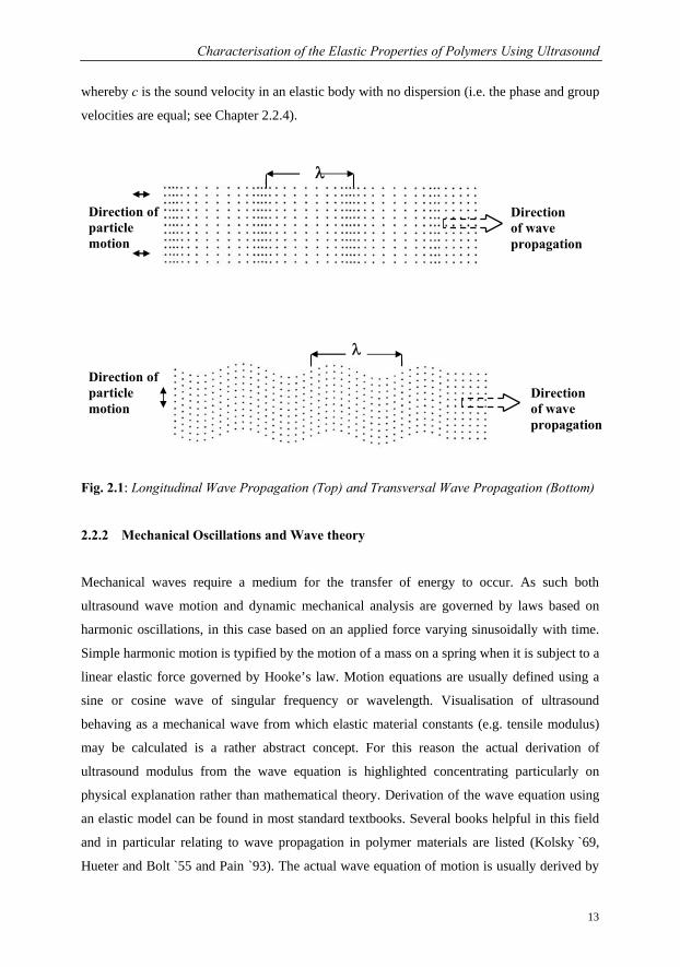
considered. Longitudinal wave propagation involves particle oscillations that occur in the
direction of the wave propagation as shown in the schematic Fig. 2.1 (on next page). Since
dilatational forces are active in these waves they are often referred to as compression or
pressure waves. Compression waves can be generated in both liquids and solids because the
energy travels through the atomic structure by a series of comparison and expansion
movements. For transverse or shear waves the particles oscillation of particles takes place at a
right or transverse angle to the direction of propagation. The particle displacement shown in
this figure is approx. 10 % of the wavelength, which is rather high and chosen for illustration
purposes. In a steel sample the particle displacement is about 1.8∗10-6 λ or 2 millionth of a
wavelength (Krautkrämer `86). Shear waves require an acoustically solid material for
effective propagation and therefore are not effectively propagated in materials such as liquids
or gases. The basic motion relationship "distance = velocity c * time t" is the key to the basic
wave relationship. Taking wavelength λ as distance, this relationship becomes λ = ct. By
using f = 1/t (where f = frequency) the standard wave relationship is formed c f λ= ,
Characterisation of the Elastic Properties of Polymers Using Ultrasound
13
whereby c is the sound velocity in an elastic body with no dispersion (i.e. the phase and group
velocities are equal; see Chapter 2.2.4).
Fig. 2.1: Longitudinal Wave Propagation (Top) and Transversal Wave Propagation (Bottom)
2.2.2 Mechanical Oscillations and Wave theory
Mechanical waves require a medium for the transfer of energy to occur. As such both
ultrasound wave motion and dynamic mechanical analysis are governed by laws based on
harmonic oscillations, in this case based on an applied force varying sinusoidally with time.
Simple harmonic motion is typified by the motion of a mass on a spring when it is subject to a
linear elastic force governed by Hooke’s law. Motion equations are usually defined using a
sine or cosine wave of singular frequency or wavelength. Visualisation of ultrasound
behaving as a mechanical wave from which elastic material constants (e.g. tensile modulus)
may be calculated is a rather abstract concept. For this reason the actual derivation of
ultrasound modulus from the wave equation is highlighted concentrating particularly on
physical explanation rather than mathematical theory. Derivation of the wave equation using
an elastic model can be found in most standard textbooks. Several books helpful in this field
and in particular relating to wave propagation in polymer materials are listed (Kolsky `69,
Hueter and Bolt `55 and Pain `93). The actual wave equation of motion is usually derived by
Direction of particle motion
λ
Direction of wave propagation
Direction of particle motion
Direction of wave propagation
λ
Characterisation of the Elastic Properties of Polymers Using Ultrasound
14 BAM-Dissertationsreihe
Eq. 2.1
Eq. 2.2
Eq. 2.3
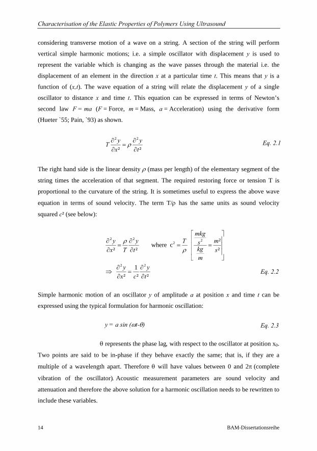
considering transverse motion of a wave on a string. A section of the string will perform
vertical simple harmonic motions; i.e. a simple oscillator with displacement y is used to
represent the variable which is changing as the wave passes through the material i.e. the
displacement of an element in the direction x at a particular time t. This means that y is a
function of (x,t). The wave equation of a string will relate the displacement y of a single
oscillator to distance x and time t. This equation can be expressed in terms of Newton’s
second law F = ma (F = Force, m = Mass, a = Acceleration) using the derivative form
(Hueter `55; Pain, `93) as shown.
2 2
² ²∂ ∂
=∂ ∂
y yTx t
ρ
The right hand side is the linear density ρ (mass per length) of the elementary segment of the
string times the acceleration of that segment. The required restoring force or tension T is
proportional to the curvature of the string. It is sometimes useful to express the above wave
equation in terms of sound velocity. The term T/ρ has the same units as sound velocity
squared c² (see below):
2 2 22
2 2
² where c ² ² ²
1 ² ² ²
mkgy y T ms
kgx T t sm
y yx c t
ρρ
⎡ ⎤⎢ ⎥∂ ∂
= = =⎢ ⎥∂ ∂ ⎢ ⎥⎣ ⎦
∂ ∂⇒ =
∂ ∂
Simple harmonic motion of an oscillator y of amplitude a at position x and time t can be
expressed using the typical formulation for harmonic oscillation:
y = a sin (ωt-θ)
θ represents the phase lag, with respect to the oscillator at position x0.
Two points are said to be in-phase if they behave exactly the same; that is, if they are a
multiple of a wavelength apart. Therefore θ will have values between 0 and 2π (complete
vibration of the oscillator). Acoustic measurement parameters are sound velocity and
attenuation and therefore the above solution for a harmonic oscillation needs to be rewritten to
include these variables.
Characterisation of the Elastic Properties of Polymers Using Ultrasound
15
Eq. 2.4
Eq. 2.6
Eq. 2.5
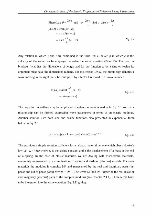
2 2 2Phase Lag and = =2 f ; also k=
( , ) sin( ) sin ( )
2 sin ( )
=
= −= −
= −
x c
y x t a ta k ct x
a ct x
π π πθ ω πλ λ λ
ω θ
πλ
Any relation in which x and t are combined in the form (ct+x) or (ct-x) in which c is the
velocity of the wave can be employed to solve the wave equation (Pain `93). The term in
brackets (ct-x) has the dimensions of length and for the function to be a sine or cosine its
argument must have the dimensions radians. For this reason (ct-x), the minus sign denotes a
wave moving to the right, must be multiplied by a factor k referred to as wave number.
2( , ) sin ( )
= sin( )
y x t a ct x
a t kx
πλ
ω
= −
−
This equation in radians may be employed to solve the wave equation in Eq. 2.1 so that a
relationship can be formed expressing wave parameters in terms of an elastic modulus.
Another solution uses both sine and cosine functions also presented in exponential form
below in Eq. 2.6.
( )(sin( ) cos( )) −= − + − = i t kxy a t kx i t kx ae ωω ω
This provides a simple solution sufficient for an elastic material i.e. one which obeys Hooke’s
law i.e. -KY =Ma where K is the spring constant and Y the displacement of a mass at the end
of a spring. In the case of plastic materials we are dealing with viscoelastic materials,
commonly represented by a combination of spring and dashpot (viscous) models. For such
materials the modulus is complex M* and represented by the real and imaginary parts (in-
phase and out of phase parts) M*=M´+ iM´´. The terms M´ and iM´´ describe the real (elastic)
and imaginary (viscous) parts of the complex modulus (see Chapter 2.1.1). These terms have
to be integrated into the wave equation (Eq. 2.1) giving:
Characterisation of the Elastic Properties of Polymers Using Ultrasound
16 BAM-Dissertationsreihe
Eq. 2.7
Eq. 2.8
Eq. 2.9
Eq. 2.10
Eq. 2.11
Eq. 2.12
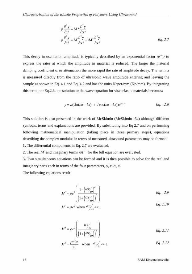
2 2
2 2 2
y yM *t² x²y y yM´ iM´
t² x² x²
∂ ∂ρ =
∂ ∂∂ ∂ ∂
ρ = +∂ ∂ ∂
This decay in oscillation amplitude is typically described by an exponential factor (e-αx ) to
express the rates at which the amplitude in material is reduced. The larger the material
damping coefficient α or attenuation the more rapid the rate of amplitude decay. The term α
is measured directly from the ratio of ultrasonic wave amplitude entering and leaving the
sample as shown in Eq. 4.1 and Eq. 4.2 and has the units Neper/mm (Np/mm). By integrating
this term into Eq.2.6, the solution to the wave equation for viscoelastic materials becomes:
(sin( ) cos( )) −= − + − xy a t kx i t kx e αω ω
This solution is also presented in the work of McSkimin (McSkimin `64) although different
symbols, terms and explanations are provided. By substituting into Eq 2.7 and on performing
following mathematical manipulation (taking place in three primary steps), equations
describing the complex modulus in terms of measured ultrasound parameters may be formed.
1. The differential components in Eq. 2.7 are evaluated.
2. The real M´ and imaginary terms iM ´´ for the full equation are evaluated.
3. Two simultaneous equations can be formed and it is then possible to solve for the real and
imaginary parts each in terms of the four parameters, ρ, c, α, ω.
The following equations result:
( )( )( )
2
' 22
' 2
1
1
when 1
cM c
c
cM c
αωρ
αω
αρ ω
⎛ ⎞−⎜ ⎟
= ⎜ ⎟⎜ ⎟+⎝ ⎠
= <<
( )( )2
2
3
1
when 1
cM c
c
c cM
αωρ
αω
ρ α αωω
⎛ ⎞⎜ ⎟
′′ = ⎜ ⎟⎜ ⎟+⎝ ⎠
′′ = <<
Characterisation of the Elastic Properties of Polymers Using Ultrasound
17
Eq. 2.14
Eq. 2.13
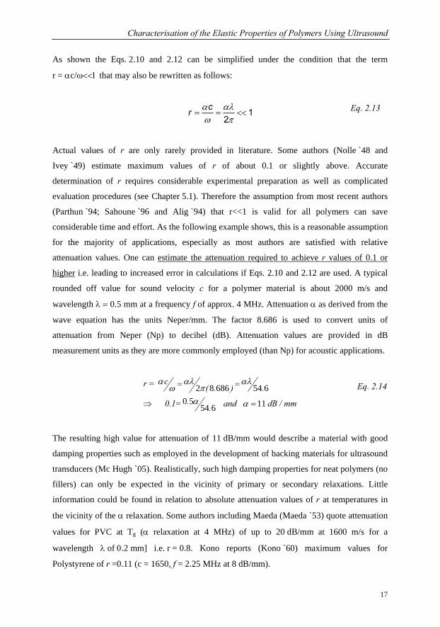
As shown the Eqs. 2.10 and 2.12 can be simplified under the condition that the term
r = αc/ω<<1 that may also be rewritten as follows:
= = <<α αλω π
12
cr
Actual values of r are only rarely provided in literature. Some authors (Nolle `48 and
Ivey `49) estimate maximum values of r of about 0.1 or slightly above. Accurate
determination of r requires considerable experimental preparation as well as complicated
evaluation procedures (see Chapter 5.1). Therefore the assumption from most recent authors
(Parthun `94; Sahoune `96 and Alig `94) that r<<1 is valid for all polymers can save
considerable time and effort. As the following example shows, this is a reasonable assumption
for the majority of applications, especially as most authors are satisfied with relative
attenuation values. One can estimate the attenuation required to achieve r values of 0.1 or
higher i.e. leading to increased error in calculations if Eqs. 2.10 and 2.12 are used. A typical
rounded off value for sound velocity c for a polymer material is about 2000 m/s and
wavelength λ = 0.5 mm at a frequency f of approx. 4 MHz. Attenuation α as derived from the
wave equation has the units Neper/mm. The factor 8.686 is used to convert units of
attenuation from Neper (Np) to decibel (dB). Attenuation values are provided in dB
measurement units as they are more commonly employed (than Np) for acoustic applications.
2 8 686 54 60 5 1154 6
= =
⇒ =
cr = ( . ) .. 0.1= and dB / mm.
α αλ αλω π
α α
The resulting high value for attenuation of 11 dB/mm would describe a material with good
damping properties such as employed in the development of backing materials for ultrasound
transducers (Mc Hugh `05). Realistically, such high damping properties for neat polymers (no
fillers) can only be expected in the vicinity of primary or secondary relaxations. Little
information could be found in relation to absolute attenuation values of r at temperatures in
the vicinity of the α relaxation. Some authors including Maeda (Maeda `53) quote attenuation
values for PVC at Tg (α relaxation at 4 MHz) of up to 20 dB/mm at 1600 m/s for a
wavelength λ of 0.2 mm] i.e. r = 0.8. Kono reports (Kono `60) maximum values for
Polystyrene of r =0.11 (c = 1650, f = 2.25 MHz at 8 dB/mm).
Characterisation of the Elastic Properties of Polymers Using Ultrasound
18 BAM-Dissertationsreihe
Eq. 2.15
Eq. 2.16
These publications provide evidence that r<<1 should not be universally assumed for all
polymers at temperatures especially in a relaxation region.
The imaginary part of the modulus M´´ is a quantity measuring the amount of energy
dissipated as heat when the material is deformed. Another parameter commonly used to
describe the materials damping properties is tan(δ) which is a measure of the internal friction
of the system. tan(δ) is defined as the ratio of the energy dissipated per cycle to the maximum
potential energy stored during a cycle i.e. tan(δ) = M´´/M´. In the field of acoustics damping
loss is also described by the Quality Factor or simply “Q” value, which is employed as a
measure of the rate at which energy decays (Pain `93). Q is simply the reciprocal of tan(δ) i.e.
Q=1/tan(δ). For acoustic measurements tan(δ) is quite easy to perceive as it can be determined
directly from the acoustic parameters as follows:
2 2tan( ) 2 and when 1
tan( ) 2
′′= = <<
′ −
= =
M ccM c
c
ω αδ α ωω α
α αλδ ω π
Interestingly, from Eqs. 2.13 and 2.15 it is observed that tan(δ) ≈ 2r. In practice r is usually
less than 0.1 apart from a few exceptions explained above. Application of tan(δ) as a
measurement parameter for describing a material’s damping properties has following
advantages (context of DMA):
does not require density values (compare to M´´) which can only be determined
from a separate experiment
can be evaluated directly from the acoustic parameters wavelength and attenuation.
can be easily compared with tan(δ) ascertained from other measurement techniques
2.2.3 Interrelation of Elastic Modulus
The velocity of longitudinal waves in a solid depends upon the dimensions of the specimen in
which the waves are travelling. The complex modulus term M* has been defined in
Chapter 2.1. If one takes a bar shaped specimen (lateral dimensions are small in comparison
to the wavelength) under tensile loading then the complex dynamic modulus M* can be
replaced by a complex tensile modulus E*. On the other hand a longitudinal wave in a
Characterisation of the Elastic Properties of Polymers Using Ultrasound
19
Eq. 2.17
Eq. 2.18
Eq. 2.19
medium compresses it and distorts it laterally. Because a solid can develop a shear force in
any direction such a lateral distortion is accompanied by a transverse shear. However, in the
case of bulk solids the longitudinal and transverse wave modes can be considered separately.
If a large (dimensions large compared to wavelength) flat poker shaped specimen is placed
under tension or compression then the complex modulus M* can be replaced by a complex
longitudinal L* or complex shear modulus G* depending on which wave mode is propagated.
The specimens employed in this project were typically a minimum of 6 times larger than the
actual wavelength of a longitudinal wave. Therefore following formulations are valid for M*
and can each be derived from the wave equation as shown.
M* M´ iM´where M * can represent L* - Longitudinal Modulus; G* - Shear Modulus K*- Bulk Modulus; E* - Youngs Modulus
= +
The various moduli can typically be interrelated using the Poisson’s ratio µp. Using the
example of a bar shaped specimen under tensile loading µp describes the relationship between
changes in length per unit length to changes in width per unit length. Poisson’s ratio can be
derived from this tensile experiment (Ferry, `80). Interrelation of G*, E* and K* and µp* is as
follows (Cowie, `91) :
p9 * * ** giving * 1
* 3 * 2 *= = −
+G K EE
G K Gμ
A three-way equation may be written relating the four basic mechanical properties.
* 3 *(1 2 *) 2(1 *) *= − = +p pE K µ µ G
Any two of these properties may be varied independently, and, conversely knowledge of any
two may be employed to calculate the remaining unknown parameters. For example, when E*
and G* in Eq. 2.19 are known then B* and µp* can be calculated. To a good approximation
Poisson’s number is µp*≈ 0.5 for soft rubbers and therefore E*=3G*. The modulus for
longitudinal waves is given by Loves Mathematical Theory of Elasticity (Love `27).
Characterisation of the Elastic Properties of Polymers Using Ultrasound
20 BAM-Dissertationsreihe
Eq. 2.20
Eq. 2.21
Eq. 2.22
L K
L K L K
= +
′ ′ ′ ′′ ′′ ′′= + = +
4Love's Theory: * * G* 3
4 4G and G (Nolle `52)3 3
This was also confirmed mathematically by rewriting Eq. 2.19 in terms of its real and
imaginary components and evaluating. Such formulations are particularly useful as one can
relate terms evaluated from experimental measurements (L´and L´´) to various other moduli.
It is evident that K´ and K´´ can only be evaluated when sound velocity and attenuation are
available for both longitudinal and shear waves. It is easy to appreciate that in liquids where it
is not possible for shear waves to propagate then L*=K*. In other words the longitudinal
modulus in liquids is equal to the bulk compression modulus (Eq. 2.19). A plot of the various
moduli for the same material will have following intensity relationship L*>K*>E*>G*
whereby G* is roughly 1/5 L* (Vogel `66). For acoustic characterisation of materials bulk
properties the interrelation of moduli is of interest, particularly as is the case here, when
comparing different measurement techniques. From the Eqs. 2.18 to 2.21 the interrelation of
L*, G* and E* can be formulated:
* 4 * 4 * ** * = ** 3 * 3*
− −=
− −
E G G EL G EE GG
Similar to Eq. 2.21, the complex modulus in Eq. 2.22 may also be replaced either by the
respective storage or loss modulus term. This was also confirmed mathematically. In the field
of material science the longitudinal modulus is a rather unfamiliar term and tensile or shear
modulus values are more common. The tensile modulus can be also obtained by longitudinal
wave propagation in thin strips or rods but this technique breaks down when the wavelength
becomes comparable to the cross-sectional dimension of the strips at higher frequencies. In
this case the longitudinal waves yield not E´ but the quantity K´+4/3G´ or simply the
longitudinal modulus L´ as in Eq. 2.20. As it is difficult to guarantee slim geometries over a
range of temperature longitudinal modulus is a much more practical value. Similarly shear
modulus can be determined using shear wave propagation but it has the distinct disadvantage
that it is very difficult to obtain accurate values in liquids or soft polymers because of their
inability to support transverse (shear) excitations.
Characterisation of the Elastic Properties of Polymers Using Ultrasound
21
2.2.4. Phase Velocity and Dispersion
The discussion so far has been limited to monochromatic waves, waves of a single frequency
and wavelength. However, it is much more common for waves to occur as a number or group
of frequency components. In the field of wave motion two main velocities that are quite
distinct although mathematically connected are of practical importance (Pain `93).
1. The phase velocity cp of a wave is the rate at which the phase of the wave propagates in the
material. This is the velocity at which the phase of any one frequency component of the wave
will propagate. You could pick one particular phase of the wave (for example the crest) and it
would appear to travel at the phase velocity. The phase velocity cp is given in terms of the
wavelength at a specific frequency or as in Eq. 2.4 in terms of the wavenumber k:
= =pc f kωλ . In mechanics a perfectly elastic material is normally represented by a spring
and the complex modulus M*=M´ as no viscous effects (M´´ or out of phase components, see
Eq. 2.7) have to be considered. In such cases wave form will be independent of frequency
(fλ is a constant) and the phase velocity cp is equal to the group velocity cg (refer to point 2).
2. A number of waves of different frequencies, wavelengths and velocities may be superposed
to form a group. The group velocity cg of a wave is the velocity with which the variations in
the shape of the wave's amplitude (known as the modulation or envelope of the wave)
propagate through space. Publications in which results are presented show that a large
difference on phase and group velocities may be observed in polymer materials (Ping `98;
Challis `00) within a limited MHz frequency range at isothermal temperatures.
A brief insight into superposition of waves and Fourier analysis principles is provided
in more detail in Chapter 4.2. Distinction of group and phase velocities is of particular interest
in dispersive medium such as polymers because the absorption properties or attenuation α
(defined in Eq. 2.8) can often change dramatically as a function of temperature. Attempts
have been made to determine suitable mathematical relations between the respective damping
for α(ω) and cp(ω) phase functions using the Kramers-Konig relations (O’Donnell `81;
Zellouf `96; Wintle `99). However such relationships are not trivial particularly in regard to
viscoelastic materials and the results are, as admitted by the last two authors cited sometimes
contradictory. Propagation of sound waves in dispersive media may distort the time domain
signal leading to a possible shift of resonance frequency, change in wavelength or signal
form. This leads to different phase shifts in different frequency components. Dispersion refers
Characterisation of the Elastic Properties of Polymers Using Ultrasound
22 BAM-Dissertationsreihe
Eq. 2.23
to the fact that the phase velocity cp of a propagating wave in dispersive media will vary with
frequency or wavelength as formulated below:
( )∂ ∂∂ ∂
= = = + = −∂ ∂ ∂ ∂
p pg p p p
c cc kc c k c
k k kω λ
λ
Dispersion may also be caused by geometry effects or scattering when heterogeneities
such as voids or crystallites occur. The frequency spectrum of the ultrasonic pulses scattered
reveal information about the scatterer’s size, shape and orientation. For heterogeneities with
sizes ranging from 1/1000 to 1/100 of the wavelength scattering is non-influential. Larger
heterogeneities if not considered in the calculations can lead to large errors in determining
modulus values using wave propagation (Krautkrämer `86). Therefore care was taken that the
epoxy samples or mixtures were homogenous enough to neglect this effect.
2.3 Time, Temperature and Frequency Effects
In the previous section the theoretical relationships between measured acoustic parameters
and the complex dynamic modulus for polymer materials, was discussed. The concepts
discussed are strictly independent of the existence of molecules; the results of those concepts
fall into the realm of continuum mechanics. The emphasis in the following is the
interpretation of the viscoelastic behaviour on a molecular scale and discussion of glass
transition phenomenon. Molecular mechanisms at least in terms of mechanical analogues are
discussed in the following which will aid in understanding time/frequency and temperature
correspondence for polymer materials. Viscoelastic materials as the name suggests exhibit a
combination of elastic and viscous behaviour. Using an amorphous polymer as an example
most textbooks describe five distinct regions of viscoelastic behaviour. The regions are
marked in Fig. 2.4 (used to demonstrate superposition principles) for a thermoplastic
(polyisobutlyene) material. Using a continued heating regime starting at low temperatures the
Glassy region refers to stiff polymer properties. Region 2 is the glass transition and describes
the transition zone from glass to rubber. Region 3 is the rubbery plateau region. As the
temperature is raised past the rubbery plateau region the polymer is marked by both rubber
elasticity and flow properties – this zone is called the rubbery flow region (4). At still higher
temperatures the liquid flow region 5 is reached. For a crosslinked polymer such as the cured
epoxy used in this work, only the first 3 regions are of interest as to a first approximation the
Characterisation of the Elastic Properties of Polymers Using Ultrasound
23
modulus will remain constant in the rubbery plateau region (see Fig. 2.2). Liquid flow will not
occur. The complex modulus is a function of time as well as temperature. Therefore, the same
viscoelastic behaviour can be observed by measuring the modulus as a function of time at
constant temperature or by measuring the modulus as a function of temperature at a constant
frequency. Modulus plotted as a function of temperature or as a function of time/frequency at
constant temperature will yield the same viscoelastic profile. The second region describes the
glass to rubber transition and results in large drop in modulus of approx. 3 orders in
magnitude and a peak in the loss modulus. This considerable variation in properties makes it
one of the most important parameters in characterising the mechanical behaviour of a cured
epoxy resin. Changes associated with the glass transition include volume and expansion
coefficients, enthalpy and mechanical properties. Experiments performed in this work take
place using different techniques but always on samples prepared in exactly the same manner
and also at low cooling rates. In the following, the influences time/frequency effects on the
determination of the glass transition are discussed from an analytical perspective.
2.3.1 Time Dependence in Mechanical (DMA) Relaxation Studies
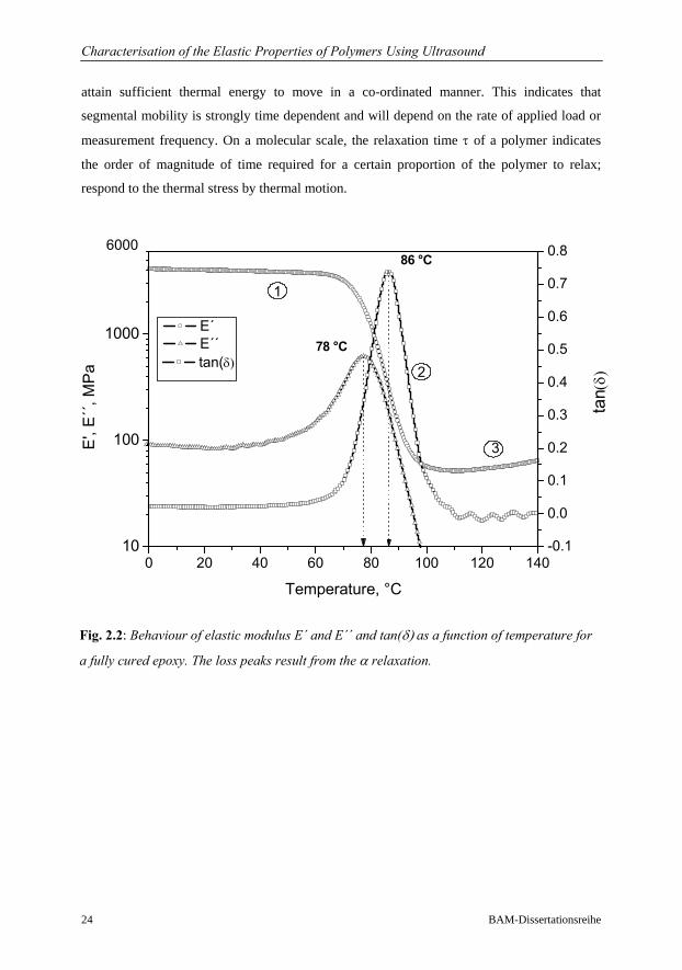
In Fig 2.2, the dynamic tensile storage E´, loss modulus E´´, and tan(δ) for a 3 point bending
experiment performed at 1 Hz on a fully cured epoxy are illustrated. DMA measurement
principles are explained in Chapter 4.3. The first 3 regions of viscoelastic behaviour for a
crosslinked polymer are clearly marked, (discussed above). At low temperatures (0 to 40 °C),
the polymer is stiff/frozen and has a high storage modulus E´ and low loss modulus E´´. The
chains are frozen in fixed positions because insufficient energy for translational and rotational
motions of the polymer segments is available. As the temperature increases, the polymer
obtains sufficient thermal energy to enable its chains to move more freely. At temperatures
larger than 100 °C the modulus decreases to about 10 MPa, a typical value for rubberlike
materials. In analogy with this process a transition occurs at temperatures between 60 to
100 °C and the loss modulus E´´ goes through a maximum. This region is referred to as the
glass rubber transition or glass transition Tg and can be qualitatively interpreted as the onset
of large scale conformational rearrangements of the polymer chain backbone (Mc Crum `67).
Frictional interaction between polymer chain segments leads to energy being dissipated as
heat and a corresponding maximum will be observed in the loss factor E´´ or tan(δ). The
temperature at which this peak maximum is observed is conventionally defined as Tg. Below
Tg only 1 to 4 chain atoms are involved in movement while above Tg 10 to 50 chain atoms
Characterisation of the Elastic Properties of Polymers Using Ultrasound
24 BAM-Dissertationsreihe
attain sufficient thermal energy to move in a co-ordinated manner. This indicates that
segmental mobility is strongly time dependent and will depend on the rate of applied load or
measurement frequency. On a molecular scale, the relaxation time τ of a polymer indicates
the order of magnitude of time required for a certain proportion of the polymer to relax;
respond to the thermal stress by thermal motion.
0 20 40 60 80 100 120 14010
100
1000
-0.1
0.0
0.1
0.2
0.3
0.4
0.5
0.6
0.7
0.8
E´ E´´
tan(
δ)
86 °C
E',
E´´
, MP
a
Temperature, °C
78 °C
6000
1
2
3
tan(δ)
Fig. 2.2: Behaviour of elastic modulus E´ and E´´ and tan(δ) as a function of temperature for
a fully cured epoxy. The loss peaks result from the α relaxation.
Characterisation of the Elastic Properties of Polymers Using Ultrasound
25
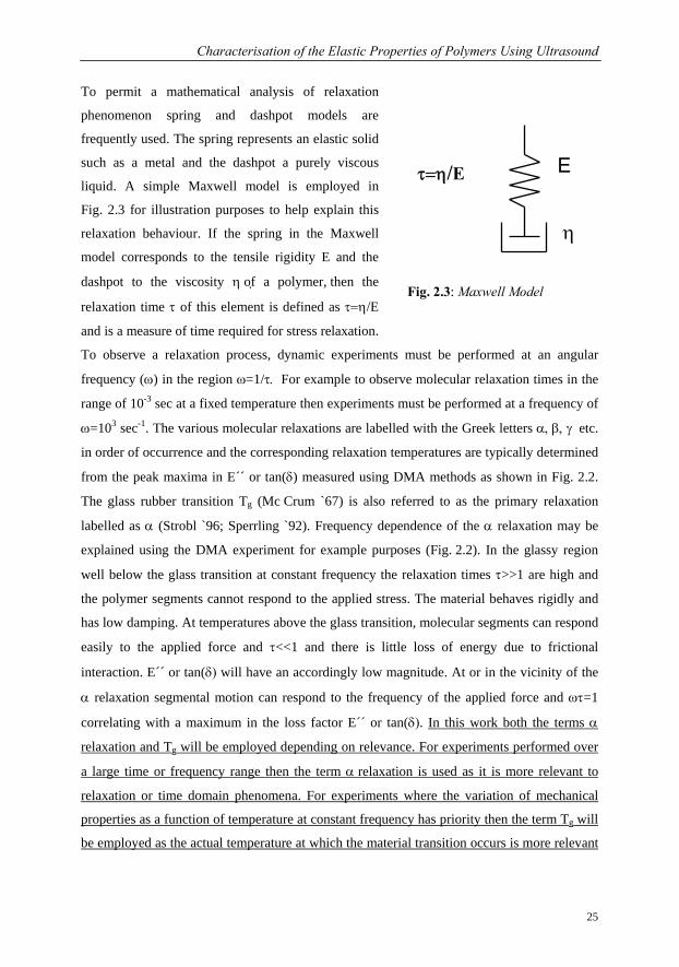
To permit a mathematical analysis of relaxation
phenomenon spring and dashpot models are
frequently used. The spring represents an elastic solid
such as a metal and the dashpot a purely viscous
liquid. A simple Maxwell model is employed in
Fig. 2.3 for illustration purposes to help explain this
relaxation behaviour. If the spring in the Maxwell
model corresponds to the tensile rigidity E and the
dashpot to the viscosity η of a polymer, then the
relaxation time τ of this element is defined as τ=η/E
and is a measure of time required for stress relaxation.
To observe a relaxation process, dynamic experiments must be performed at an angular
frequency (ω) in the region ω=1/τ. For example to observe molecular relaxation times in the
range of 10-3 sec at a fixed temperature then experiments must be performed at a frequency of
ω=103 sec-1. The various molecular relaxations are labelled with the Greek letters α, β, γ etc.
in order of occurrence and the corresponding relaxation temperatures are typically determined
from the peak maxima in E´´ or tan(δ) measured using DMA methods as shown in Fig. 2.2.
The glass rubber transition Tg (Mc Crum `67) is also referred to as the primary relaxation
labelled as α (Strobl `96; Sperrling `92). Frequency dependence of the α relaxation may be
explained using the DMA experiment for example purposes (Fig. 2.2). In the glassy region
well below the glass transition at constant frequency the relaxation times τ>>1 are high and
the polymer segments cannot respond to the applied stress. The material behaves rigidly and
has low damping. At temperatures above the glass transition, molecular segments can respond
easily to the applied force and τ<<1 and there is little loss of energy due to frictional
interaction. E´´ or tan(δ) will have an accordingly low magnitude. At or in the vicinity of the
α relaxation segmental motion can respond to the frequency of the applied force and ωτ=1
correlating with a maximum in the loss factor E´´ or tan(δ). In this work both the terms α
relaxation and Tg will be employed depending on relevance. For experiments performed over
a large time or frequency range then the term α relaxation is used as it is more relevant to
relaxation or time domain phenomena. For experiments where the variation of mechanical
properties as a function of temperature at constant frequency has priority then the term Tg will
be employed as the actual temperature at which the material transition occurs is more relevant
E
η
τ=η/E
Fig. 2.3: Maxwell Model
Characterisation of the Elastic Properties of Polymers Using Ultrasound
26 BAM-Dissertationsreihe
Eq. 2.24
than the actual molecular relaxation times. This differentiation is common procedure in
standard literature related to polymer science (Murayama `78; Ferry `86).
2.3.2 TTS Theory: Time Temperature Superposition
As stated, determination of the modulus for a viscoelastic material will depend on frequency
or timescale and temperature of a given experiment. However, only a small range of
viscoelastic response manifests itself during an experimentally accessible time range. The
accessible time scale for stress relaxation experiments lies in the 101 to 106 sec range but
obviously a wider range would be desirable. Observations on viscoelastic materials showed
that changing stress relaxation times is equivalent to changing temperature (Leaderman `43).
Using this information a composite isothermal curve covering the required temperature range
can be constructed from data collected at different temperatures (Fig. 2.4). This is
accomplished by translation of small curves along the logarithmic time axis until they are all
superimposed to form a large master curve. Stress relaxations data at one temperature can be
superimposed on data taken at a different temperature merely by shifting the creep curves.
The time scale (relaxation time) at each individual measurement temperature is multiplied by
a shift factor aT. The shift factor is estimated by shifting each individual component curve so
that it can be superimposed on a reference curve at time tref. The component curves represent
measurements at different constant temperatures. The factor aT is chosen so that the
component curves can be joined onto the reference curve at tref forming a smooth profile. The
curve obtained at each temperature is shifted by an amount aT:
ref T Tref
log log = loga a− ⇒ =tt t
t
The so-called master curve formed illustrates the relaxation behaviour over the generated time
scale at the chosen reference temperature. The relaxation rate equals the rate of transitions
between two conformational states. The observed activation energy Ea has to be identified
with the height of the energy barrier which has to be passed over during this change. In
Fig. 2.4 a logarithmic plot of the shift factor against temperature is illustrated. Over a small
temperature interval such a plot will often be linear indicating a thermally activated process,
with a relaxation time being given by the Arrhenius law:
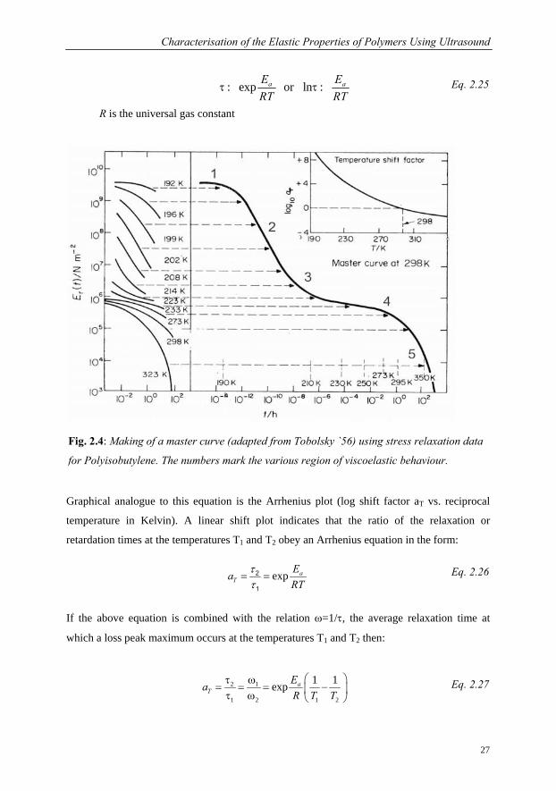
Characterisation of the Elastic Properties of Polymers Using Ultrasound
27
Eq. 2.25
Eq. 2.26
Eq. 2.27
R is the universal gas constant
Graphical analogue to this equation is the Arrhenius plot (log shift factor aT vs. reciprocal
temperature in Kelvin). A linear shift plot indicates that the ratio of the relaxation or
retardation times at the temperatures T1 and T2 obey an Arrhenius equation in the form:
If the above equation is combined with the relation ω=1/τ, the average relaxation time at
which a loss peak maximum occurs at the temperatures T1 and T2 then:
2 1
1 2 1 2
1 1exp ⎛ ⎞τ ω
= = = −⎜ ⎟τ ω ⎝ ⎠a
TEaR T T
exp or lna aE ERT RT
τ τ: :
exp aT
EaRT
ττ
= =2
1
Fig. 2.4: Making of a master curve (adapted from Tobolsky `56) using stress relaxation data
for Polyisobutylene. The numbers mark the various region of viscoelastic behaviour.
1
Characterisation of the Elastic Properties of Polymers Using Ultrasound
28 BAM-Dissertationsreihe
Eq. 2.28
Using this equation the influence of high measurement frequencies (ultrasound - MHz) on the
determination of Tg can be estimated. As an example, if one considers an increase in
frequency of one decade (e2.303) then the above equation can be reformulated as follows:
2.303
1 2
1 2
1 1exp
1 1 2.303
a
a
EeR T T
RandT T E
⎛ ⎞= −⎜ ⎟
⎝ ⎠⎛ ⎞
− =⎜ ⎟⎝ ⎠
Estimated values of Ea = 84 kcal/mol (355 kJ/mol) for the α relaxation process in polystyrene
can be found in the literature (Sperling `92). Also an approximate value of Tg = 373 K for
polystyrene that was obtained using low frequency techniques (Brydson `90) can be placed
into Eq. 2.28 by letting T2 = Tg. In this manner T1 is determined and yields a value of 7.5 or in
other words Tg will be observed at a temperature approx. 7.5 K higher for every decade
increase in frequency. This value is also commonly quoted in textbooks on the basis of DEA
measurements (Sperling `92 and Cowie `91). However, following points should be considered
before using accepting that such a general rule is valid for the majority for polymers:
1. This rule will be very dependent on the actual activation energy of the individual
polymer (see Eq. 2.27).
2. For the majority of polymers if Tg is plotted against the reciprocal of frequency it will
not exhibit linear behaviour but will be slightly curved. In this case the Williams
Landel Ferry WLF equation is better suited for modelling the frequency behaviour.
Some authors (Aklonis `72) suggest using such plots to differentiate between primary
and secondary relaxations. The former exhibiting WLF behaviour and the latter
Arrhenius dependence Polystyrene is one of the few exceptions where the Arrhenius
equation is better suited to describe frequency dependence of observed Tg.
The derivation of this WLF equation is based on free volume principles (Ferry `80) and is
illustrated in Eq. 2.28. According to Ferry (Ferry `80) the constants C1 and C2 can be
calculated experimentally by plotting (T-Tref )/log aT against T-Tref: whereby T refers to
temperature and Tref is a constant reference. From the slope s and the intercept i of the
resulting line the constants are calculated: C1 = 1/s and C2=i/s.
Characterisation of the Elastic Properties of Polymers Using Ultrasound
29
Eq. 2.29
Eq. 2.30
1
2
( )log ref
Tref
C T Ta
C T T− −
=+ −
According to investigations performed by the WLF author if a temperature approx 50 K
above the Tg is chosen then C1 = 8.86 and C2 =101.6 K are constants independent of polymer.
It is more common is to reduce relaxation, temperature or creep data to the glass transition
temperature Tg. In such experiments Tg = Tref and if no experimental data is available then C1
and C2 are chosen as 17.44 and 51.6 °K respectively. Nowadays, these values are normally
taken as universal for polymers (prerequisite Tg = Tref). According to Strobl, (Strobl `96) this
is not true and the constants C1 and C2 are material dependent parameters that will normally
vary in the ranges C1 = 14 to 18 and C2 = 30 to 70 K. For the example illustrated in Fig. 2.4,
the Tg of Polyisobutylene is given as 202 K (at low frequencies). If C1 and C2 are chosen as
17.44 and 51.6 °K then a shift factor of approx. 5 °C for every decade increase in frequency
can be estimated. Therefore the rule of thumb describing the influence of measurement
frequency on Tg should just be taken as a rough estimate as it typically varies somewhere
between 5 and 8 K per decade and will depend on whether an Arrhenius or WLF model is
used. It is obviously better, where possible, to determine the constants C1 and C2
experimentally. In order to obtain an analytical expression that can be used to estimate the
activation energy Ea from the WLF equation, Aklonis (Aklonis `72) placed the Arrhenius law
written in the form shown in Eq. 2.25 back into the WLF Eq. 2.28 using aT as the common
term. This expression is used to determine the activation energy and will be very dependent
on the actual glass transition temperature. If the universal constants are employed for C1 and
C2 then the equation can be rewritten as 6.47 (Tg²), which means that for a polymer with a α
relaxation process at 353 K, an activation energy of 800 kJ/mol is obtained. The activation
energy will obviously increase the higher the glass transition of the polymer i.e. will depend
on the measurement frequency of the experiment.
R = Universal gas constant .
( )2
21 2 12
22
2.303 2.303a g
g
C C RT CE = RT CC T T
⎛ ⎞= ⎜ ⎟
+ − ⎝ ⎠
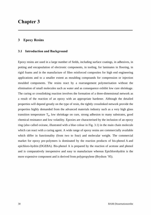
30 BAM-Dissertationsreihe
Chapter 3
3 Epoxy Resins
3.1 Introduction and Background
Epoxy resins are used in a large number of fields, including surface coatings, in adhesives, in
potting and encapsulation of electronic components, in tooling, for laminates in flooring, in
rigid foams and in the manufacture of fibre reinforced composites for high end engineering
applications and to a smaller extent as moulding compounds for compression or injection
moulded components. The resins react by a rearrangement polymerisation without the
elimination of small molecules such as water and as consequence exhibit low cure shrinkage.
The curing or crosslinking reaction involves the formation of a three-dimensional network as
a result of the reaction of an epoxy with an appropriate hardener. Although the detailed
properties will depend greatly on the type of resin, the tightly crosslinked network provide the
properties highly demanded from the advanced materials industry such as a very high glass
transition temperature Tg, low shrinkage on cure, strong adhesion to many substrates, good
chemical resistance and low volatility. Epoxies are characterised by the inclusion of an epoxy
ring (also called oxirane, illustrated with a blue colour in Fig. 3.1) in the main chain molecule
which can react with a curing agent. A wide range of epoxy resins are commercially available
which differ in functionality (from two to four) and molecular weight. The commercial
market for epoxy pre-polymers is dominated by the reaction products of bis-phenol A and
epichloro-hydrin (DGEBA). Bis-phenol A is prepared by the reaction of acetone and phenol
and is comparatively inexpensive and easy to manufacture whereas Epichlorohydrin is the
more expensive component and is derived from polypropylene (Brydson `95).
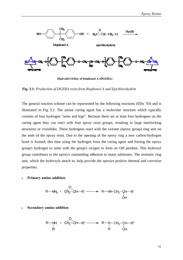
Epoxy Resins
31
The general reaction scheme can be represented by the following reactions (Ellis `93) and is
illustrated in Fig. 3.2. The amine curing agent has a molecular structure which typically
consists of four hydrogen “arms and legs”. Because there are at least four hydrogens on the
curing agent they can react with four epoxy resin groups, resulting in large interlocking
structures or crosslinks. These hydrogens react with the oxirane (epoxy group) ring unit on
the ends of the epoxy resin. Due to the opening of the epoxy ring a new carbon-hydrogen
bond is formed, this time using the hydrogen from the curing agent and freeing the epoxy
group's hydrogen to unite with the group's oxygen to form an OH pendant. This hydroxyl
group contributes to the epoxy's outstanding adhesion to many substrates. The aromatic ring
unit, which the hydroxyls attach to, help provide the epoxies positive thermal and corrosion
properties.
• Primary amine addition
• Secondary amine addition
Diglycidyl Ether of bisphenol A (DGEBA)
Fig. 3.1: Production of DGEBA resin from Bisphenol A and Epichlorohydrin
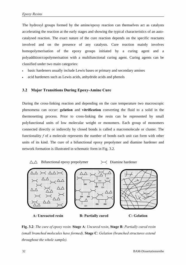
Epoxy Resins
32 BAM-Dissertationsreihe
The hydroxyl groups formed by the amine/epoxy reaction can themselves act as catalysts
accelerating the reaction at the early stages and showing the typical characteristics of an auto-
catalysed reaction. The exact nature of the cure reaction depends on the specific reactants
involved and on the presence of any catalysts. Cure reaction mainly involves
homopolymerisation of the epoxy groups initiated by a curing agent and a
polyaddition/copolymerisation with a multifunctional curing agent. Curing agents can be
classified under two main categories:
• basic hardeners usually include Lewis bases or primary and secondary amines
• acid hardeners such as Lewis acids, anhydride acids and phenols
3.2 Major Transitions During Epoxy-Amine Cure
During the cross-linking reaction and depending on the cure temperature two macroscopic
phenomena can occur: gelation and vitrification converting the fluid to a solid in the
thermosetting process. Prior to cross-linking the resin can be represented by small
polyfunctional units of low molecular weight or monomers. Each group of monomers
connected directly or indirectly by closed bonds is called a macromolecule or cluster. The
functionality f of a molecule represents the number of bonds each unit can form with other
units of its kind. The cure of a bifunctional epoxy prepolymer and diamine hardener and
network formation is illustrated in schematic form in Fig. 3.2.
A: Unreacted resin B: Partially cured C: Gelation
Bifunctional epoxy prepolymer Diamine hardener
OH
OH OH
OH OH OH
OH OH
OH
OH
Fig. 3.2: The cure of epoxy resin. Stage A: Uncured resin, Stage B: Partially cured resin
(small branched molecules have formed), Stage C: Gelation (branched structures extend
throughout the whole sample).
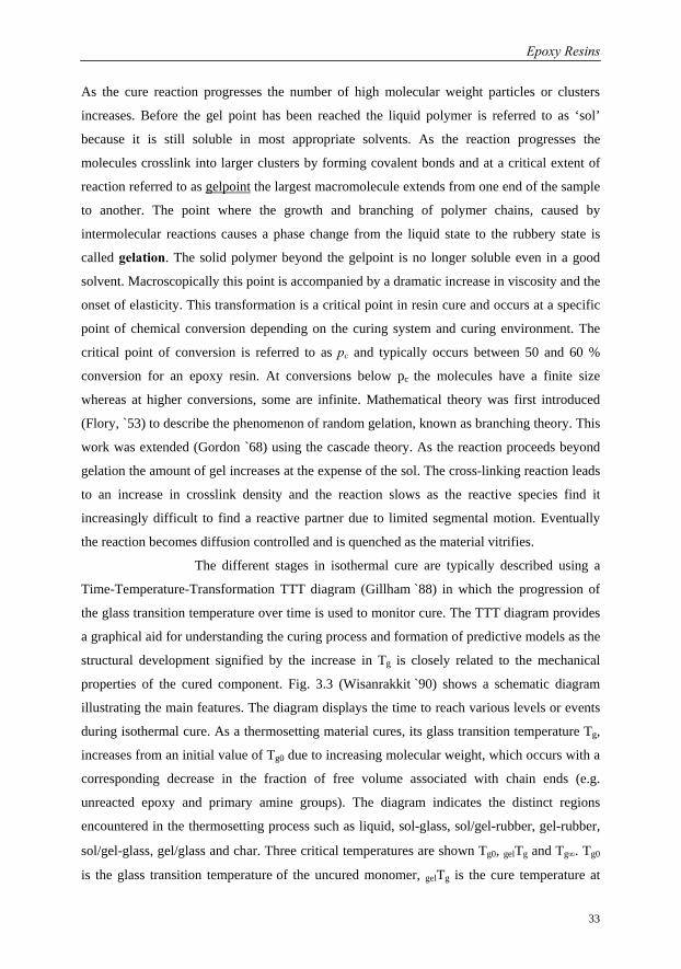
Epoxy Resins
33
As the cure reaction progresses the number of high molecular weight particles or clusters
increases. Before the gel point has been reached the liquid polymer is referred to as ‘sol’
because it is still soluble in most appropriate solvents. As the reaction progresses the
molecules crosslink into larger clusters by forming covalent bonds and at a critical extent of
reaction referred to as gelpoint the largest macromolecule extends from one end of the sample
to another. The point where the growth and branching of polymer chains, caused by
intermolecular reactions causes a phase change from the liquid state to the rubbery state is
called gelation. The solid polymer beyond the gelpoint is no longer soluble even in a good
solvent. Macroscopically this point is accompanied by a dramatic increase in viscosity and the
onset of elasticity. This transformation is a critical point in resin cure and occurs at a specific
point of chemical conversion depending on the curing system and curing environment. The
critical point of conversion is referred to as pc and typically occurs between 50 and 60 %
conversion for an epoxy resin. At conversions below pc the molecules have a finite size
whereas at higher conversions, some are infinite. Mathematical theory was first introduced
(Flory, `53) to describe the phenomenon of random gelation, known as branching theory. This
work was extended (Gordon `68) using the cascade theory. As the reaction proceeds beyond
gelation the amount of gel increases at the expense of the sol. The cross-linking reaction leads
to an increase in crosslink density and the reaction slows as the reactive species find it
increasingly difficult to find a reactive partner due to limited segmental motion. Eventually
the reaction becomes diffusion controlled and is quenched as the material vitrifies.
The different stages in isothermal cure are typically described using a
Time-Temperature-Transformation TTT diagram (Gillham `88) in which the progression of
the glass transition temperature over time is used to monitor cure. The TTT diagram provides
a graphical aid for understanding the curing process and formation of predictive models as the
structural development signified by the increase in Tg is closely related to the mechanical
properties of the cured component. Fig. 3.3 (Wisanrakkit `90) shows a schematic diagram
illustrating the main features. The diagram displays the time to reach various levels or events
during isothermal cure. As a thermosetting material cures, its glass transition temperature Tg,
increases from an initial value of Tg0 due to increasing molecular weight, which occurs with a
corresponding decrease in the fraction of free volume associated with chain ends (e.g.
unreacted epoxy and primary amine groups). The diagram indicates the distinct regions
encountered in the thermosetting process such as liquid, sol-glass, sol/gel-rubber, gel-rubber,
sol/gel-glass, gel/glass and char. Three critical temperatures are shown Tg0, gelTg and Tg∞. Tg0
is the glass transition temperature of the uncured monomer, gelTg is the cure temperature at
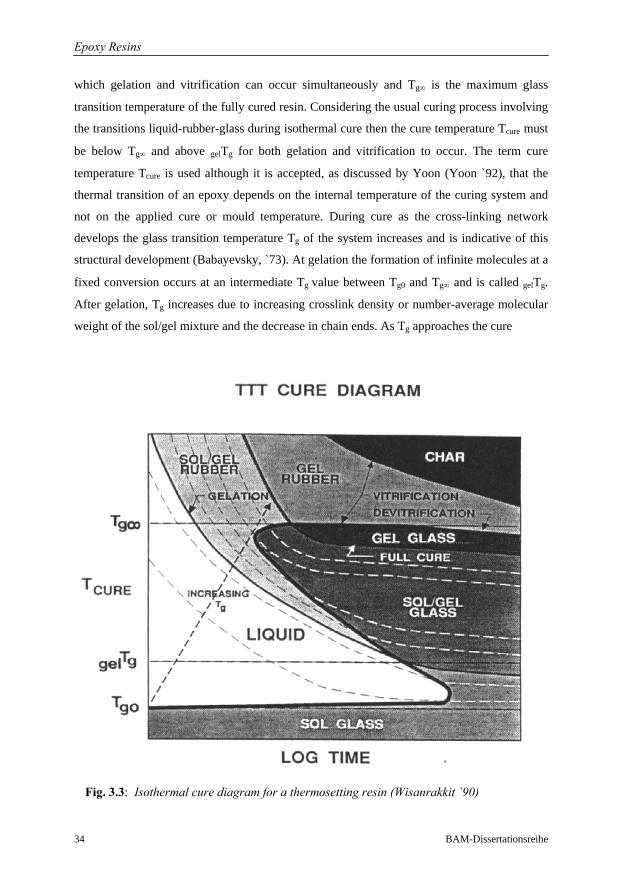
Epoxy Resins
34 BAM-Dissertationsreihe
which gelation and vitrification can occur simultaneously and Tg∞ is the maximum glass
transition temperature of the fully cured resin. Considering the usual curing process involving
the transitions liquid-rubber-glass during isothermal cure then the cure temperature Tcure must
be below Tg∞ and above gelTg for both gelation and vitrification to occur. The term cure
temperature Tcure is used although it is accepted, as discussed by Yoon (Yoon `92), that the
thermal transition of an epoxy depends on the internal temperature of the curing system and
not on the applied cure or mould temperature. During cure as the cross-linking network
develops the glass transition temperature Tg of the system increases and is indicative of this
structural development (Babayevsky, `73). At gelation the formation of infinite molecules at a
fixed conversion occurs at an intermediate Tg value between Tg0 and Tg∞ and is called gelTg.
After gelation, Tg increases due to increasing crosslink density or number-average molecular
weight of the sol/gel mixture and the decrease in chain ends. As Tg approaches the cure
Fig. 3.3: Isothermal cure diagram for a thermosetting resin (Wisanrakkit `90)
Epoxy Resins
35
temperature, the material enters the glass transition region and is defined to vitrify when Tg
equals Tcure. The gradual cessation of the reaction marks the transition from rubber to glass.
This transition is defined as vitrification and is considered the end of cure. If the cure
temperature is above the Tg of the fully cured material, Tg∞ by definition, the material cannot
vitrify at Tcure and in this case the chemical kinetics will govern the progress of the reaction. If
the temperature is held for long periods of time at Tg∞ then devitrification which is caused by
degradation may occur as well as char formation at even higher temperatures. One particular
feature of the TTT diagram that should not be overlooked is the S-shaped curve form between
the boundary lines Tg0 and Tg showing that an increase in reaction rate will mean that the cure
time for a particular event or transition will decrease decrease with increasing cure
temperature. The time axis has a logarithmic scale so that for example a sol/gel glass state
may only realistically be achieved over a period of days or weeks. In a typical commercial
curing cycle the resin will pass from a liquid to a gel/rubber state and vitrify (otherwise it
would deform on removal from a mould). Cure times vary very broadly from days to minutes
depending on the manufacturing process for example hand lay-up or automated resin injection
moulding.
3.3 Cure Modelling: Kinetics and Chemorheology
During the cure of a thermosetting resin a number of complex chemical and physical changes
occur as the material turns from a viscous liquid to a highly crosslinked solid. These changes
are reflected in the chemorheological characteristics of each individual resin system and
determine the optimum set of process parameters for the production of a material. Adequate
models combining cure kinetics and chemorheology are a primary component of
thermosetting composites manufacturing simulations. Two main approaches to modelling can
be distinguished:
1. Phenomenological or empirical modelling: tends to ignore the chemical reaction
mechanisms and utilises approximate relationships which usually resemble
chemical kinetic expressions. This is the more traditional method of searching for
a rate law and its activation parameters which describes the overall reaction within
a range of conversion as well as possible.
Epoxy Resins
36 BAM-Dissertationsreihe
2. Mechanistic modelling: Overall reaction is broken down by a combination of
reaction steps with constant activation parameters. The single steps can be
described by all known rate laws for homogenous and heterogeneous reactions. A
reaction scheme representing the curing mechanism is selected which can be
described by a mathematical reaction rate equation system. The fact that a multiple
parameter estimation for a non-analytical expression of resin kinetics makes
mechanistic models sometimes unattractive. However, new evaluation programs
(Flammersheim `02) provide help in this area. The formal kinetic models as a rule
do not correspond to real elementary reactions but provide very high fitting values
i.e. are helpful in understanding real reaction behaviour.
The complexity as well as the importance of cure kinetics is reflected by innumerable
publications and models which can be found relating to points 1 and 2. Despite the effort that
has been expended on cure kinetics of epoxy, there is still no general model which can be
applied to the cure of all epoxy resins. As I am interested in comparing various
physiochemical analytical techniques, the suitability of applying phenomenological models
for comparison purposes was looked at.
A wide variety of models are available to aid in analysis and prediction of the curing
reaction. Choice of kinetic or chemorheological depends largely on area of interest and
analytical technique. Every chemical reaction is associated with a certain heat of reaction. It
therefore follows that the heat flow rate is proportional to the rate of reaction. Kinetic
modelling is therefore typically based on calorimetric measurement techniques. Techniques
sensitive to network formation or progress of modulus or viscosity naturally come under the
title chemorheology. A linear relationship exists between conversion and Tg (related to
structure development) for the kinetic part of the crosslinking reaction so that both kinetics
and chemorheological models are known to be closely interlinked (Gillham `79). Although
this relationship still exists it breaks down signified by non linearity in the latter part of cure
at high conversion values (> 60%). At this point the reaction becomes diffusion controlled i.e.
at temperatures Tcure < Tg. Traditionally many kinetic evaluation techniques were directed at
finding a rate law and its parameters which describes the overall reaction within a conversion
range. As discussed in Chapter 3.1 Epoxy cure may take place in a series of reaction steps
e.g. catalysis and autocatalysis may even occur simultaneously and published models are
therefore usually material specific and not universal. This point will be discussed in the
following section starting with the basis equation for rate constant calculation and therefore
kinetic analysis, known as the Arrhenius equation.
Epoxy Resins
37
-
0
EaR Tk A e ×= ×
0
ln aEkA R T
= −⋅
3.3.1 Application of the Arrhenius Equation
Chemical reactions are normally associated with a certain heat of reaction. It therefore follows
that the heat flow rate is proportional to the progress of the reaction. This process is normally
explained by the barrier theory and the activation energy. The basic assumptions are that for a
reaction to occur, reactant species must come together and secondly must have sufficient
energy to form a product (overcome an energy barrier). The Swedish chemist Arrhenius (1859
to 1927) postulated that the energetic term (Ea) correlates with the enthalpic activation barrier
for the reaction and can be described by the following equations:
or logarithmic form
A0 = Pre-exponential term; k = rate of reaction
R = Gas constant; Ea = Activation Energy (J/mol)
The actual equation was formed from observations on the effect of temperature on reaction
rate. It was found empirically that a plot of log k vs. 1/T produced a linear relationship. Thus a
plot of ln k vs. (1/T) will provide a line with a slope of – Ea/R and an intercept of ln A. The
(extrapolated) cut with the ln y-axis provides directly the value of the pre-exponential factor
A, and the slope of the straight line gives the activation energy Ea. (Standard: ASTM E698).
One of the primary objectives of kinetic analysis is parameterizing the temperature
dependence of the reaction rate. Although both Arrhenius parameters A and Ea are needed to
describe the temperature dependence, the discussion of the reaction kinetics tends to focus on
the activation energy. This is probably because the temperature sensitivity of the reaction rate
is predominantly determined by Ea, whereas A plays the role of a scaling parameter, which
determines the absolute value of the reaction rate.
3.3.2 Reaction Rate Laws in Kinetic Modelling
Every quantitative kinetic analysis starts with the determination of a continuous
sequence of concentration of reactants versus time data. The goal of kinetics is to measure a
concentration of a species at a particular time during the reaction so that a rate law may be
determined. When thermoanalytic techniques such as Differential Scanning Calorimetry DSC
Eq. 3.1
Epoxy Resins
38 BAM-Dissertationsreihe
( ) tQtQ
α∞
=
are used for the investigation of kinetic problems, the concentrations of the reactants which
are often unknown are usually replaced by degrees of reaction α that are typically obtained
from DSC measurements (Borchardt `57). In this case the measured heat of reaction is Q. For
a curing reaction the degree of conversion α is calculated from the heat of reaction and is
determined from the ratio of the partial area Qt to the total area Q∞ of an exothermal DSC
peak and α ranges from 0 to 1.:
Three general methods (Höhne `03) can be described for the determination of kinetic
parameters although numerous variations are available. The direct method following the
procedure of Borchardt (Borchardt `57) is used here. A general reaction rate k(T) law may be
written as follows:
( ) ( ) where ( ) (1 )nd k T f fdtα α α α= ⋅ = −
f(α) is assumed to be a function of conversion independent of temperature. The value n
describes the order of a reaction with respect to a certain reactant. It is defined as the power to
which the concentration (or conversion) term in the above rate equation is raised. If the
correct reaction order is chosen then a linear plot of (1-α) vs. reaction time should result
(Standard: DIN 53 529). At present different calorimeter manufacturers offer linear regression
software so that multiple experiments at different heating rates can be quickly and efficiently
analysed and values for n, lnA and EA can be determined. For an epoxy amine system such as
described in this work the reaction is quite complicated and cannot be described by just one
rate constant. The cure process can be split into three regions: kinetic control with initial small
activation energies which can be attributed to the initial catalytic or autocatalytic reaction. As
the reaction advances, the autocatalysis reaction diminishes giving way to the non-catalytic
epoxy amine addition reaction with a consequent increase in the activation energy of the
reacting system and a transition to the diffusion control region with an accordingly strong
decrease in reaction rate. For such multiple step reactions it is generally accepted that the
Arrhenius equation, which describes a linear relationship between reaction rate and
temperature, can only be used as a reaction rate law in a limited range. Even so, most authors
(Guibe `96; Karkanas `97) agree that this equation provides a good linear fit to experimental
Eq. 3.2
Eq. 3.3
Epoxy Resins
39
1 2(1 ) (1 )n m nd k c kdtα α α α= ⋅ ⋅ − + ⋅ ⋅ −
1 1 1
overall chem diffk k k= +
data up to about 60 to 65 % conversion. Some authors argue that because both catalysed and
non-catalysed reactions (may have different activation energies) can occur simultaneously for
epoxy amine reactions a true description of multiple step reactions is risky using Arrhenius
approximations because they may actually hinder further advances towards understanding the
true reaction mechanism. This statement should be approached with care as even with modern
software the large number of free parameters used in kinetic modelling, mean that often only
a very experienced user could come to any conclusion about the “real” reaction mechanism.
The advantage of using more complex models which employ an overall rate law is that they
allow for catalytic and autocatalytic reactions, and often provide a more accurate fit to
experimental data. One such popular model employs the Sourour-Kamal (Sourour `71)
equation:
where c is the concentration of the catalyst, n and m are formal reaction
orders, k1 is the rate constant for the initial reaction including effects of catalysts and k2
describes the autocatalysed reaction. The reaction orders n and m are mathematical fitting
parameters and as such the physiochemical validity is questionable. For an epoxy amine
crosslinking systems this equation only characterises the initial stages of the reaction.
Deviations are observed in the later stages such that the reaction is decelerated or even
quenched due to restrictions in chain mobility by the tightening molecular network. This
process is referred to as vitrification and can also be described in terms of state as a rubber to
glass transition Tg. In the vicinity of vitrification diffusion of the reactive species will become
very slow and governs the curing reaction. The separate reaction mechanisms can then be
divided into: pure chemical reaction and diffusion control. For both phenomenological and
mechanistic models at high conversions, modification to Sourour-Kamal (Eq.3.4) kinetic
model has to be introduced. Therefore to achieve a complete evaluation of reaction kinetics
the above model must also take into account the more or less complete change from
chemically to diffusion controlled reaction steps. The most frequently used integration
formulation is given below (Rabinowitch `37).
Eq. 3.4
Eq. 3.5
Epoxy Resins
40 BAM-Dissertationsreihe
1 10
2 2
0
( ) 2.303 ( )( )log ln ln( ) ( ) ( )
exp
− −= = +
+ − + +
⎛ ⎞−⎜ ⎟
⎝ ⎠
cure g cure gdd d
d g cure g cure g
dd d
cure
C T T C T Tk T or k kk T C T T C T T
Ewhere k =A RT
As usual the term kchem describes the pure chemical reaction (k1, k2) with no
diffusion considerations. Several approaches to determine kdiff are discussed in the literature
(Karkanas `97; Höhne `03). However, whilst the chemical rate constant follows an Arrhenius
dependence this is not the case for the diffusion rate constant. Since diffusion is a measure of
the structure development, it must follow the changes both in Tg and in cure temperature.
(Karkanas `00). One of the more popular techniques to determine kdiff uses a modified WLF
equation (Enns `83) that is also described by Wise (Wise `97). The parameters C1 and C2 are
presumed to be constants with respective values of 40 and 51.6 K (Ferry `80). kd is the
diffusion rate constant and kd0 = k(Tg) is taken as the diffusion rate constant at Tg.Tcure is the
cure temperature.
In particular Karkanas (Karkanas `00) provides a convincing argument
based on experimental data from several epoxy resins that C1 and C2 do not remain constant
during cure, further complicating evaluation procedures. When diffusion becomes significant
the rate constants (k1 and k2) in Eq. 3.4 should be replaced by apparent rate constants, which
are a combination of the diffusion rate constant and the chemical reaction constants shown in
Eq. 3.5 and estimated using Eq. 3.6. Taking these factors into consideration the Sourour-
Kamal equation (Eq. 3.4) can now be modified to include diffusion control (Karkanas `96).
As shown the equations and models typically employed to describe the
reaction kinetics of a curing epoxy can become quite complex. Taking all factors into
consideration Skordos (Skordos `00) stated that his colleague (Karkanas `97), derived non-
linear equations with 7 to 11 free parameters to fit experimental data obtained from four
different epoxy systems. The fits achieved using these models are excellent, but it is relatively
easy to loose the overview. Such models have been shown to function quite well for a specific
resin system however any alteration of the resin system will require the reiteration of the
laborious model parameter estimation procedure. In such cases the models become more
mathematically based and have limited validity in rigorous chemistry terms. This is the main
argument for using a mechanistic model whereby a reaction scheme representing the curing
Eq. 3.6
Epoxy Resins
41
mechanism is selected which can be described by a mathematical reaction rate equation
system. The disadvantage is that mechanistic results are very dependent on adequacy (in
particular in terms of quantity) of experimental data. This traditional form of searching for
rate laws and activation parameters for the overall reaction is as shown complicated and time
consuming and therefore evaluation programs independent on which modelling system is
used are very useful.
3.3.3 Network formation and Glass Transition
Up to this point the objective was to find a relatively simple a rate law that is best suited to
describe the chemical reaction and that could be employed to model the measured ultrasound
results used in this work. All models presented rely almost exclusively on data obtained from
DSC experiments. Rheological models describing the development of the modulus or
viscosity throughout cure are much rarer. This is most likely due to the fact that most
rheological instruments are limited in their measurement range and a model is only as good as
the experimental data available. Therefore models only exist for prediction of viscosity
behaviour up to about gelation point (50 to 60 % conversion). The most common equation
used to model viscosity or rheological measurements in this range is an adapted WLF
equation (Williams `55), adapted to describe the variation of viscosity of thermoplastics with
temperature (Ferry `80). It should be noted that in the original WLF formulation the
temperature is replaced by cure temperature Tcure. The equation implies that if we know the
viscosity η at some temperature ηT then we can estimate the viscosity at Tg where C1 and C2
are normally taken as constant with respective values of 17.44 and 51.6 K.
Unlike thermoplastics, thermosets undergo a polymerisation reaction so that a change of
structure occurs and C1 and C2 will become as material dependent parameters (Mijovic `89).
The rate of network formation is a function of kinetics which in turn is a function of
temperature and time. Hence to correctly employ Eq. 3.7 one requires (a) the increase in glass
transition as a function of network formation i.e. degree of cure and (b) variation of C1 and C2
as a function of cure temperature from viscosity experiments. Karkanas provides
(Karkanas `00) provides a detailed explanation on the calculation of C1 and C2 using linear
1
2
( )ln
( )−
= −+ −
c gT
g c g
C T TC T T
ηη
Eq. 3.7
Epoxy Resins
42 BAM-Dissertationsreihe
regression mathematics. Taking these factors into consideration the authors (Mijovic `89 and
Karkanas `00) were able to provide excellent models for viscosity advancement for a range of
epoxy resins. Of course the modelled data, is just as good as the experimental results
available, which means only the early stages of cure (about 50 to 60 % conversion) were
considered, so that such models are not suitable for predicted diffusion behaviour i.e. have not
been employed to model vitrification.
Therefore a different model or more importantly experimental analysis technique is required
to describe the relationship between glass transition and conversion or extent of reaction. It is
well known that in the case of epoxy/amine reactive mixtures the relationship between Tg and
conversion is independent of cure temperature. The most comprehensive expression that
correlates segmental motion and chemical conversion with Tg is the following expression
(Adabbo `82 and DiBenedetto `87):
αλλα)1(1)( 0
0 −−
−+= ∞ gg
gg
TTTT where λ=
m
x
FF
where α is the conversion at the glass transition; glass transition temperatures of the
uncross-linked Tg0, partial- Tg and fully cross-linked Tg∞ polymer and Fx/Fm is the ratio of
segmental mobility’s for the polymer at Tg0 and Tg∞.. Theoretically the adjustable parameter λ
is equated to the ratio of the respective heat capacities cp for the initial mixture cp0 and the
fully cured network cp∞ (Pascault `90; Georjon`93).
This is an important statement as quite often segmental motion activity can only be estimated
whereas heat capacities can be measured using modern calorimetric techniques. It has been
suggested (Karkanas `00) that a single λ value is able to describe all characteristic cure
behaviour for a specific resin. For each new thermosetting polymer analysed it will have to be
determined experimentally. The results from the above authors show a significant amount of
scatter when the experimental results, degree of conversion α versus Tg are fitted with the
experimental model obtained from the Eqs. 3.8 and Eq. 3.9. The authors attribute this to the
lower sensitivity of conversion in the later stages of cure.
Eq. 3.8
∞ =p
p0
cc
λ Eq. 3.9
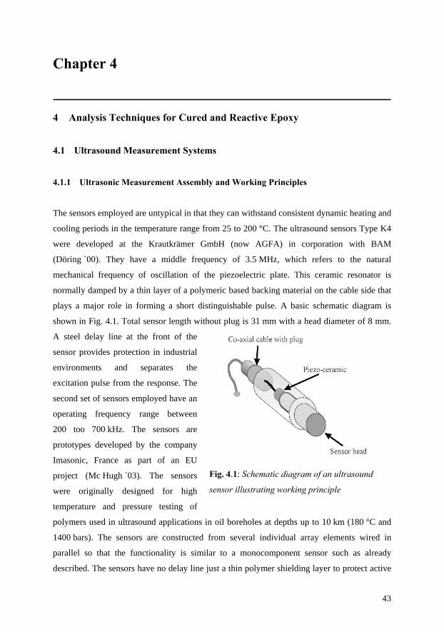
43
Chapter 4
4 Analysis Techniques for Cured and Reactive Epoxy
4.1 Ultrasound Measurement Systems
4.1.1 Ultrasonic Measurement Assembly and Working Principles
The sensors employed are untypical in that they can withstand consistent dynamic heating and
cooling periods in the temperature range from 25 to 200 °C. The ultrasound sensors Type K4
were developed at the Krautkrämer GmbH (now AGFA) in corporation with BAM
(Döring `00). They have a middle frequency of 3.5 MHz, which refers to the natural
mechanical frequency of oscillation of the piezoelectric plate. This ceramic resonator is
normally damped by a thin layer of a polymeric based backing material on the cable side that
plays a major role in forming a short distinguishable pulse. A basic schematic diagram is
shown in Fig. 4.1. Total sensor length without plug is 31 mm with a head diameter of 8 mm.
A steel delay line at the front of the
sensor provides protection in industrial
environments and separates the
excitation pulse from the response. The
second set of sensors employed have an
operating frequency range between
200 too 700 kHz. The sensors are
prototypes developed by the company
Imasonic, France as part of an EU
project (Mc Hugh `03). The sensors
were originally designed for high
temperature and pressure testing of
polymers used in ultrasound applications in oil boreholes at depths up to 10 km (180 °C and
1400 bars). The sensors are constructed from several individual array elements wired in
parallel so that the functionality is similar to a monocomponent sensor such as already
described. The sensors have no delay line just a thin polymer shielding layer to protect active
Fig. 4.1: Schematic diagram of an ultrasound
sensor illustrating working principle
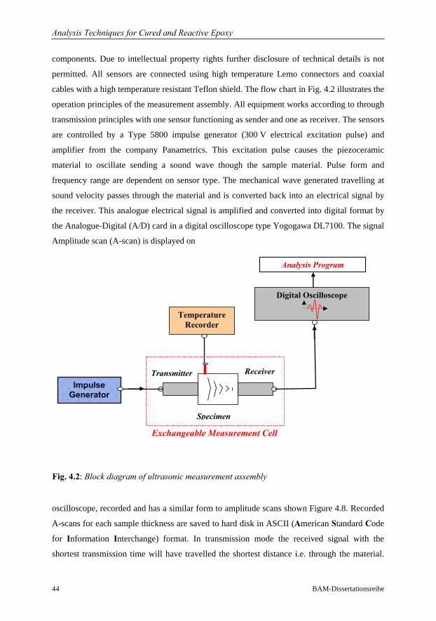
Analysis Techniques for Cured and Reactive Epoxy
44 BAM-Dissertationsreihe
components. Due to intellectual property rights further disclosure of technical details is not
permitted. All sensors are connected using high temperature Lemo connectors and coaxial
cables with a high temperature resistant Teflon shield. The flow chart in Fig. 4.2 illustrates the
operation principles of the measurement assembly. All equipment works according to through
transmission principles with one sensor functioning as sender and one as receiver. The sensors
are controlled by a Type 5800 impulse generator (300 V electrical excitation pulse) and
amplifier from the company Panametrics. This excitation pulse causes the piezoceramic
material to oscillate sending a sound wave though the sample material. Pulse form and
frequency range are dependent on sensor type. The mechanical wave generated travelling at
sound velocity passes through the material and is converted back into an electrical signal by
the receiver. This analogue electrical signal is amplified and converted into digital format by
the Analogue-Digital (A/D) card in a digital oscilloscope type Yogogawa DL7100. The signal
Amplitude scan (A-scan) is displayed on
oscilloscope, recorded and has a similar form to amplitude scans shown Figure 4.8. Recorded
A-scans for each sample thickness are saved to hard disk in ASCII (American Standard Code
for Information Interchange) format. In transmission mode the received signal with the
shortest transmission time will have travelled the shortest distance i.e. through the material.
Impulse Generator
Analysis Program
Digital Oscilloscope
Temperature Recorder
Specimen
Transmitter Receiver
Exchangeable Measurement Cell
Fig. 4.2: Block diagram of ultrasonic measurement assembly
Analysis Techniques for Cured and Reactive Epoxy
45
The technique has the added advantage that interference caused by surface waves, reflections
at material boundaries and electrical noise (because two separate electrical lines are used) will
not be as strong as for a reflection technique.
4.1.2 Design and Function: Testing Equipment and Ultrasound Sensors
4.1.2.1 Thermal Analysis at 2 to 7 MHz on a fully Cured Epoxy
Fig. 4.3 illustrates a measurement cell designed for testing solid polymers. The cell contains
4 sensors i.e. two measurement lines in through transmission. Two solid polymer samples
with different thicknesses are measured simultaneously using this technique. The
measurement cell was originally designed for use in high pressure autoclaves and therefore
has a threaded (not visible) steel adapter. Both samples were clamped using personal
judgement (hand tight) without applying any excessive pressure. The main criterion was that
no deformation of samples occurred. Both top and bottom sensor rows can be adjusted
individually and the clamp adjusts the bottom cylindrical back plate (on the adapter side). The
opposite aluminium cylindrical plate on the side of the clamp is stationary. This means the
assembly can be adjusted quite finely to obtain optimal contact with the samples while at the
same time ensuring samples of varying thicknesses can be safely clamped in position. For
heating or cooling experiments the whole cell is placed in a silicon oil bath. The clamped
samples are heated to approximately 180 °C over a 2 hour period and held at this temperature
for 30 minutes before the experiment is started. This is to ensure that the samples are fully
cured. As it is difficult to control the temperature in a dynamic heating run, the oil-bath
containing cell and samples is heated to 200 °C and cools slowly in air, to room temperature.
Metal components are constructed from aluminium. Although one measurement can take up
to 8 hours before the oil-bath reaches room temperature, this technique has the advantage that
samples with different thicknesses should have equivalent homogeneous temperatures.
Temperature was monitored using a Type K thermocouple wire placed in the vicinity of the
epoxy samples Another thermocouple wire is placed in the oil-bath itself to monitor
differences. The thermocouple is connected to a WE 4000 measuring station from Yogogawa
which is connected to the computer by an RS232 interface. Samples are prepared by pouring
the epoxy mixture at room temperature into a 12 mm diameter cylindrical silicon mould. The
prepared samples are then sanded down to thicknesses of approx. 4 mm and 8 mm. Sample
thickness is checked before and after each measurement to account for sample deformation or
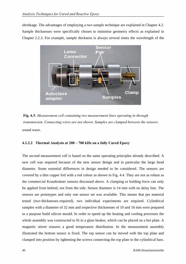
Analysis Techniques for Cured and Reactive Epoxy
46 BAM-Dissertationsreihe
shrinkage. The advantages of employing a two sample technique are explained in Chapter 4.2.
Sample thicknesses were specifically chosen to minimise geometry effects as explained in
Chapter 2.2.3. For example, sample thickness is always several times the wavelength of the
sound wave.
4.1.2.2 Thermal Analysis at 200 – 700 kHz on a fully Cured Epoxy
The second measurement cell is based on the same operating principles already described. A
new cell was required because of the new sensor design and in particular the large head
diameter. Some essential differences in design needed to be considered. The sensors are
covered by a thin copper foil with a red colour as shown in Fig. 4.4. They are not as robust as
the commercial Krautkrämer sensors discussed above. A clamping or holding force can only
be applied from behind, not from the side. Sensor diameter is 14 mm with no delay line. The
sensors are prototypes and only one sensor set was available. This means that per material
tested (two thicknesses required), two individual experiments are required. Cylindrical
samples with a diameter of 32 mm and respective thicknesses of 10 and 16 mm were prepared
in a purpose build silicon mould. In order to speed up the heating and cooling processes the
whole assembly was constructed to fit in a glass beaker, which can be placed on a hot plate. A
magnetic stirrer ensures a good temperature distribution. In the measurement assembly
illustrated the bottom sensor is fixed. The top sensor can be moved with the top plate and
clamped into position by tightening the screws connecting the top plate to the cylindrical bars.
Fig. 4.3: Measurement cell containing two measurement lines operating in through
transmission. Connecting wires are not shown. Samples are clamped between the sensors.
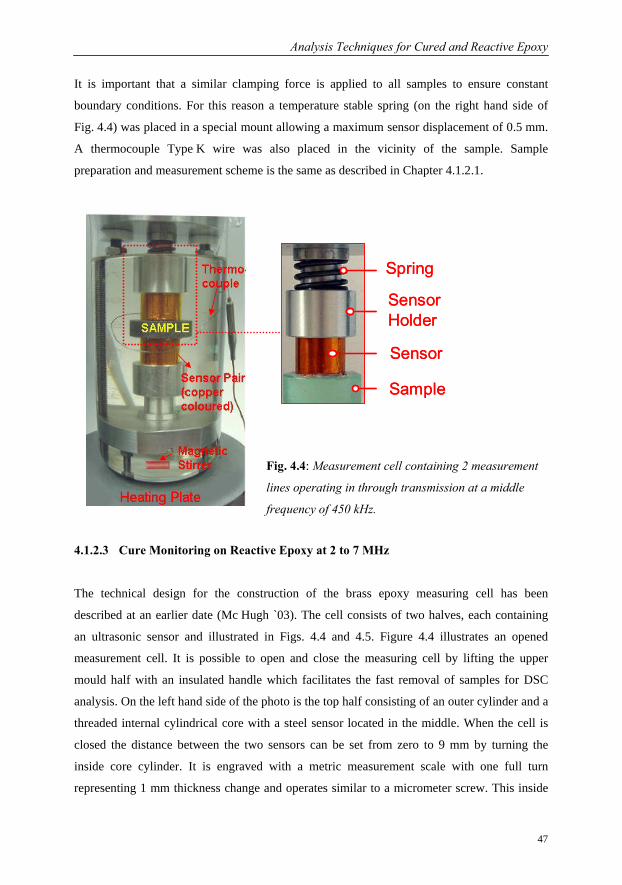
Analysis Techniques for Cured and Reactive Epoxy
47
It is important that a similar clamping force is applied to all samples to ensure constant
boundary conditions. For this reason a temperature stable spring (on the right hand side of
Fig. 4.4) was placed in a special mount allowing a maximum sensor displacement of 0.5 mm.
A thermocouple Type K wire was also placed in the vicinity of the sample. Sample
preparation and measurement scheme is the same as described in Chapter 4.1.2.1.
4.1.2.3 Cure Monitoring on Reactive Epoxy at 2 to 7 MHz
The technical design for the construction of the brass epoxy measuring cell has been
described at an earlier date (Mc Hugh `03). The cell consists of two halves, each containing
an ultrasonic sensor and illustrated in Figs. 4.4 and 4.5. Figure 4.4 illustrates an opened
measurement cell. It is possible to open and close the measuring cell by lifting the upper
mould half with an insulated handle which facilitates the fast removal of samples for DSC
analysis. On the left hand side of the photo is the top half consisting of an outer cylinder and a
threaded internal cylindrical core with a steel sensor located in the middle. When the cell is
closed the distance between the two sensors can be set from zero to 9 mm by turning the
inside core cylinder. It is engraved with a metric measurement scale with one full turn
representing 1 mm thickness change and operates similar to a micrometer screw. This inside
Sample
Sensor Holder
Spring
Sensor
Sample
Sensor Holder
Spring
Sensor
Fig. 4.4: Measurement cell containing 2 measurement
lines operating in through transmission at a middle
frequency of 450 kHz.
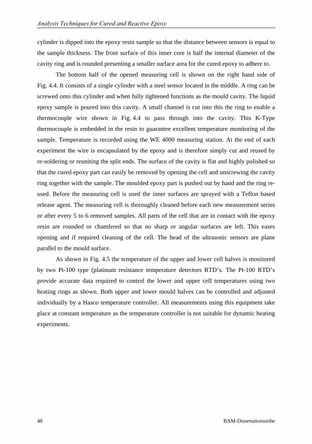
Analysis Techniques for Cured and Reactive Epoxy
48 BAM-Dissertationsreihe
cylinder is dipped into the epoxy resin sample so that the distance between sensors is equal to
the sample thickness. The front surface of this inner core is half the internal diameter of the
cavity ring and is rounded presenting a smaller surface area for the cured epoxy to adhere to.
The bottom half of the opened measuring cell is shown on the right hand side of
Fig. 4.4. It consists of a single cylinder with a steel sensor located in the middle. A ring can be
screwed onto this cylinder and when fully tightened functions as the mould cavity. The liquid
epoxy sample is poured into this cavity. A small channel is cut into this the ring to enable a
thermocouple wire shown in Fig. 4.4 to pass through into the cavity. This K-Type
thermocouple is embedded in the resin to guarantee excellent temperature monitoring of the
sample. Temperature is recorded using the WE 4000 measuring station. At the end of each
experiment the wire is encapsulated by the epoxy and is therefore simply cut and reused by
re-soldering or reuniting the split ends. The surface of the cavity is flat and highly polished so
that the cured epoxy part can easily be removed by opening the cell and unscrewing the cavity
ring together with the sample. The moulded epoxy part is pushed out by hand and the ring re-
used. Before the measuring cell is used the inner surfaces are sprayed with a Teflon based
release agent. The measuring cell is thoroughly cleaned before each new measurement series
or after every 5 to 6 removed samples. All parts of the cell that are in contact with the epoxy
resin are rounded or chamfered so that no sharp or angular surfaces are left. This eases
opening and if required cleaning of the cell. The head of the ultrasonic sensors are plane
parallel to the mould surface.
As shown in Fig. 4.5 the temperature of the upper and lower cell halves is monitored
by two Pt-100 type (platinum resistance temperature detectors RTD’s. The Pt-100 RTD’s
provide accurate data required to control the lower and upper cell temperatures using two
heating rings as shown. Both upper and lower mould halves can be controlled and adjusted
individually by a Hasco temperature controller. All measurements using this equipment take
place at constant temperature as the temperature controller is not suitable for dynamic heating
experiments.
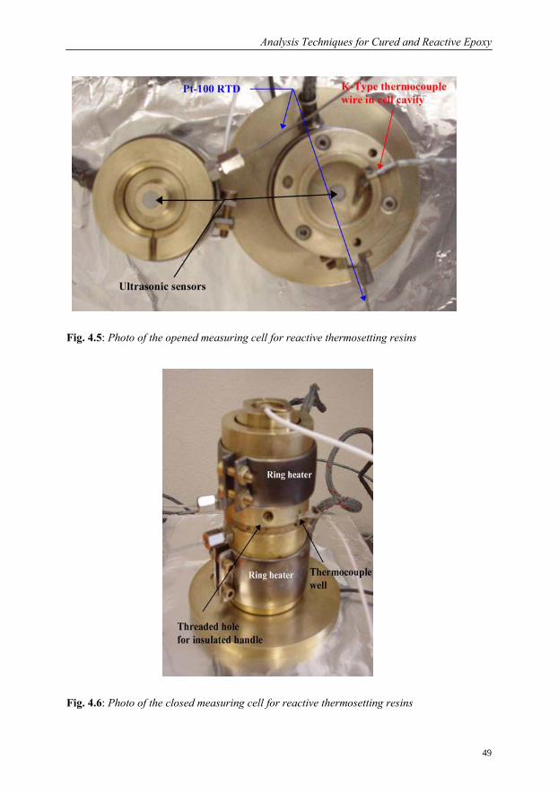
Analysis Techniques for Cured and Reactive Epoxy
49
Fig. 4.5: Photo of the opened measuring cell for reactive thermosetting resins
Fig. 4.6: Photo of the closed measuring cell for reactive thermosetting resins
Analysis Techniques for Cured and Reactive Epoxy
50 BAM-Dissertationsreihe
4.2 Ultrasound Generation and Detection
The amplitude of a sound wave passing through different media will decrease continuously
with distance as it loses mechanical energy. In the discussion on wave theory and interrelation
to mechanical modulus, it was shown that sound velocity in the medium is related to the
elastic constants whereas attenuation depends primarily on the inelastic or viscous properties.
Two principle forms of acoustic losses are of particular relevance to this study:
1. Scattering processes or reflections on material boundaries causes a decrease in wave
amplitude. Such losses are a result of different material impedance values as the wave
propagates through one medium to another (see Eqs. 4.3 and 4.4 on following page).
Particularly during dynamic temperature runs (from 20 to 200 °C) it is expected that
the impedance difference between, for example, the surface of a steel sensor and a
polymer will not remain constant. The polymer will exhibit a much larger change in
sound velocity than a metal in this temperature range. .
2. Absorption of wave energy mainly caused by internal friction or relaxation effects,
and hysteresis (frequency dependence of wave propagation in polymers). Essentially
this refers to dissipative dispersion or any mechanism leading to the conversion of
acoustic energy to thermal energy that results in a loss of wave amplitude (increase in
attenuation).
Great care has been taken in preparing the samples so that no inhomengenities or voids
occur and therefore related scattering effects can be neglected. The measured acoustic
attenuation will be influenced strongly by a combination of both the above effects. To
understand which mechanism actually leads to a reduction in signal amplitude, it was
necessary to find a means to quantify or separate each effect. This may be achieved
experimentally. The attenuation α in the polymer sample is calculated from the ratio of the
ultrasonic wave amplitude entering the sample Ai and exiting the sample Ae taking into
consideration sample thickness d (Eqs. 4.1 and 4.2). A schematic illustration of measurement
setup is also shown in Fig. 4.7.
Eq. 4.1
Eq. 4.2 ln
i e
e
i
dA = A e
A1 d A
− α⋅
α =
Analysis Techniques for Cured and Reactive Epoxy
51
The measured amplitude value Ae will be influenced by several factors including frequency,
thickness of sample and boundary losses already discussed. In order to determine the actual
material attenuation, other sources of acoustic losses need to be accounted for. One of the
main sources causing a loss in amplitude occurs at the boundary. Each material has its own
characteristic sound velocity c and density ρ, which are related by the acoustic impedance Z.
The reflection factor R at the boundary of two materials with respective impedances Z1 and Z2
can be calculated as follows:
The problem with reflectivity on material boundaries is aggravated by the fact that the
temperature during experiments on the cured epoxy is not constant. This means accurate
evaluation of attenuation is difficult using one sample because material dependent impedance
values and reflectivity e.g. between steel sensor and epoxy boundaries will very probably vary
disproportionately over the temperature range employed. If two identical samples with
different thicknesses are used the reflectivity factor R may be considered identical (Fig. 4.7)
and the attenuation may be calculated directly from the amplitude ratio of the samples. The
attenuation α is calculated from the measured signal amplitude A1 and A2 after transmission
through the respective samples with thickness d1 and d2. Attenuation α in damped oscillations
measures the rate at which the amplitude decays and is described by an exponential function
e-αd as shown in Eq. 4.1. In the following Eq. 4.2 is adapted to the two sample measuring
technique as follows and presented in Neper and dB units.
Also sound velocity c is calculated using the two sample technique by measuring the sample
transmission times τ1 and τ2 for different thicknesses d1 and d2 as shown in Eq.4.7.
2 1
2 1
( ) - or c ( ) -
d thickness d dcTransmission Timeτ τ τ
= =
Eq. 4.5 2
1 2 1
2
1 2 1
A 1ln [Np/mm]A
A 120 log [dB/mm]A
d d
d d
α
α
=−
=−
Eq. 4. 3
Eq. 4. 4 2 1
1 2
-
= ρ
=+
Z c
Z ZRZ Z
Eq. 4.7
Eq. 4.6
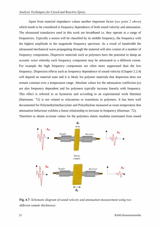
Analysis Techniques for Cured and Reactive Epoxy
52 BAM-Dissertationsreihe
Apart from material impedance values another important factor (see point 2 above)
which needs to be considered is frequency dependence of both sound velocity and attenuation.
The ultrasound transducers used in this work are broadband i.e. they operate at a range of
frequencies. Typically a sensor will be classified by its middle frequency, the frequency with
the highest amplitude in the magnitude frequency spectrum. As a result of bandwidth the
ultrasound mechanical wave propagating through the material will also consist of a number of
frequency components. Dispersive materials such as polymers have the potential to damp an
acoustic wave whereby each frequency component may be attenuated to a different extent.
For example the high frequency components are often more suppressed than the low
frequency. Dispersion effects such as frequency dependence of sound velocity (Chapter 2.2.4)
will depend on material state and it is likely for polymer materials that dispersion does not
remain constant over a temperature range. Absolute values for the attenuation coefficient (α)
are also frequency dependent and for polymers typically increase linearly with frequency.
This effect is referred to as hysteresis and according to an experimental work Hartman
(Hartmann `72) is not related to relaxations or transitions in polymers. It has been well
documented for Polymethylmethacrylate and Polyethylene measured at room temperature that
attenuation behaviour exhibits a linear relationship to increase in frequency (Hartman `72).
Therefore to obtain accurate values for the polymers elastic modulus (estimated from sound
Epoxy sample
d2
A0 A2 Receiver Sender
Sender Receiver A1
A0
d1
Fig. 4.7: Schematic diagram of sound velocity and attenuation measurement using two
different sample thicknesses

Analysis Techniques for Cured and Reactive Epoxy
53
velocity and attenuation), phase and group velocities of waves in dispersive media as well as
frequency dependent attenuation need be determined. This is achieved using spectral analysis
of the broadband pulses. At each temperature an oscillogram or amplitude scan (A-scan) is
recorded and analysed. For this specific application using a two component technique no
evaluation software was available facilitating the evaluation of attenuation and sound velocity
as a function of frequency. For this reason a program was written by J. Mc Hugh and
J. Bartusch at BAM using the Labview® computer language from National Instruments. In
the following paragraphs the basic background and evaluation principles used for this analysis
software are described starting with a basic description of Fast Fourier Transformation FFT
analysis.
4.2.1 Spectral Analysis using Fast Fourier Transformation FFT Software
The advantage of using the Labview® program language is that several Digital Signal
Processing DSP functions such as the FFT analysis are available in the program library and
can be adapted to specific problems. The following passages provide a step by step
breakdown on how the phase velocity and attenuation are evaluated using this software. The
hardware setup for recording the A-scans has been discussed in Chapter 4.1.1. To demonstrate
how the program functions a real evaluation example is provided for measurements using the
two sample set-up shown in Fig. 4.3. Two fully cured epoxy samples 10 and 16 mm thick are
placed in the experimental assembly illustrated. The assembly is placed in an oil bath which is
used as a heating medium. The sensors operate in the kHz range and have a middle frequency
of 450 kHz. An A-scan is recorded at specific temperatures using a digital oscilloscope
described in section 4.1 and loaded into the Labview program. The ASCII files loaded contain
the recorded amplitude (curve form) information with 1002 sample points containing
amplitude values. Time information is obtained from the oscilloscope measured window
settings, in this example the A-scan is measured in the 0 to 20 µs time window. As different
time and amplification settings may be employed, these settings are also written into the
source file name – white box above the A-Scan in Figure 4.8 e.g. 20dB_25°C_10mm.
Window settings and amplification are then typed into settings boxes clearly marked with
yellow and black colours above the A-Scan.
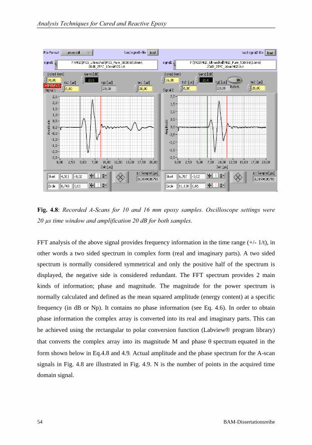
Analysis Techniques for Cured and Reactive Epoxy
54 BAM-Dissertationsreihe
Fig. 4.8: Recorded A-Scans for 10 and 16 mm epoxy samples. Oscilloscope settings were
20 µs time window and amplification 20 dB for both samples.
FFT analysis of the above signal provides frequency information in the time range (+/- 1/t), in
other words a two sided spectrum in complex form (real and imaginary parts). A two sided
spectrum is normally considered symmetrical and only the positive half of the spectrum is
displayed, the negative side is considered redundant. The FFT spectrum provides 2 main
kinds of information; phase and magnitude. The magnitude for the power spectrum is
normally calculated and defined as the mean squared amplitude (energy content) at a specific
frequency (in dB or Np). It contains no phase information (see Eq. 4.6). In order to obtain
phase information the complex array is converted into its real and imaginary parts. This can
be achieved using the rectangular to polar conversion function (Labview® program library)
that converts the complex array into its magnitude M and phase θ spectrum equated in the
form shown below in Eq.4.8 and 4.9. Actual amplitude and the phase spectrum for the A-scan
signals in Fig. 4.8 are illustrated in Fig. 4.9. N is the number of points in the acquired time
domain signal.
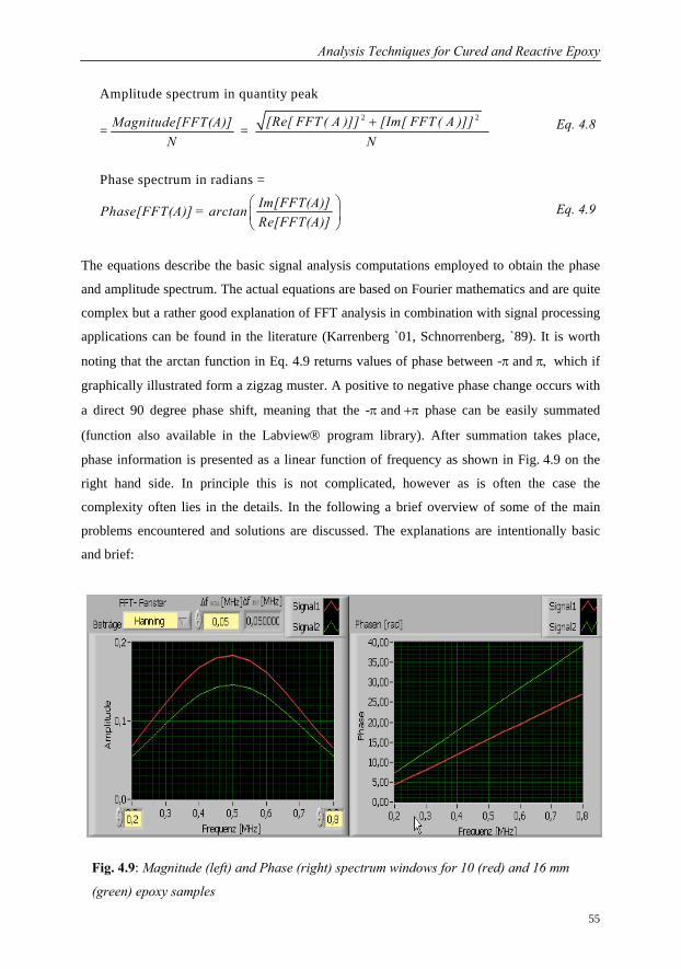
Analysis Techniques for Cured and Reactive Epoxy
55
The equations describe the basic signal analysis computations employed to obtain the phase
and amplitude spectrum. The actual equations are based on Fourier mathematics and are quite
complex but a rather good explanation of FFT analysis in combination with signal processing
applications can be found in the literature (Karrenberg `01, Schnorrenberg, `89). It is worth
noting that the arctan function in Eq. 4.9 returns values of phase between -π and π, which if
graphically illustrated form a zigzag muster. A positive to negative phase change occurs with
a direct 90 degree phase shift, meaning that the -π and +π phase can be easily summated
(function also available in the Labview® program library). After summation takes place,
phase information is presented as a linear function of frequency as shown in Fig. 4.9 on the
right hand side. In principle this is not complicated, however as is often the case the
complexity often lies in the details. In the following a brief overview of some of the main
problems encountered and solutions are discussed. The explanations are intentionally basic
and brief:
Eq. 4.8
Eq. 4.9
2 2
Amplitude spectrum in quantity peak
= =
Phase spectrum in radians =
[Re[ FFT ( A )]] [Im[ FFT ( A )]]Magnitude[FFT(A)]N N
Im[FFT(A)]Phase[FFT(A)] = arctanRe[FFT(A)]
+
⎛ ⎞⎜ ⎟⎝ ⎠
Fig. 4.9: Magnitude (left) and Phase (right) spectrum windows for 10 (red) and 16 mm
(green) epoxy samples
Analysis Techniques for Cured and Reactive Epoxy
56 BAM-Dissertationsreihe
• The FFT analysis provides frequency information about phase and amplitude over an
almost unlimited frequency spectrum. However only 1002 sample points are available
and therefore resolution will suffer, if as in the case here only a tiny part of the
spectrum (200 to 800 kHz) is analysed.
If only the spectrum, as in this example, between 2 and 7 MHz is considered the
number of sample points and therefore resolution is reduced considerably. The resolution
(distance between points) in the frequency spectrum is given by Δf=1/(N⋅Δt), where Δt is the
sampling period, Δf frequency period and N is the number of points in the acquired time
domain signal. The sampling frequency will determine the frequency bandwidth of the
spectrum and for a given sampling frequency, the number of points acquired in the recorded
time domain signal determines the resolution frequency. Simply, if one wishes to increase
frequency resolution, increase the number of points acquired at a given sampling frequency.
As the A-scan (time domain) is recorded and not analysed in real time, it can be loaded into
the program and easily padded with extra points through interpolation. In this case the
amplitude before the green line is set to exactly zero and padded by 10000 zero amplitude
sample points having the effect of spectrum smoothing and increasing the frequency
resolution.
• The green and red cursor line can be shifted with the mouse so that only the signal of
interest is analysed (as shown in Fig. 4.8). For signal analysis of the frequency
spectrum a Hanning window was used. Why?
Under normal signal acquisition conditions it is difficult to obtain a nicely scaled,
single sided spectrum. This has largely to do with the fact that the FFT algorithm assumes that
signals contained in the time domain are periodic at intervals that are a multiple of the original
signal. If the time domain has a non-integral number of cycles, this assumption is violated and
spectral leakage occurs. Another way of looking at this case is that the non-integral cycle of
the frequency component does not correspond exactly to one of the spectrum frequency lines.
This may eventually lead to a smearing of the spectrum known as spectral leakage eventually
leading to some amplitude error in the frequency peak. This is a common problem in Digital
Signal Processing DSP and several window functions are available for analysis, which help
avoid such discontinuities. The windowing of input data is mathematically equivalent to
convolving the original spectrum with the spectrum of the window function. All window
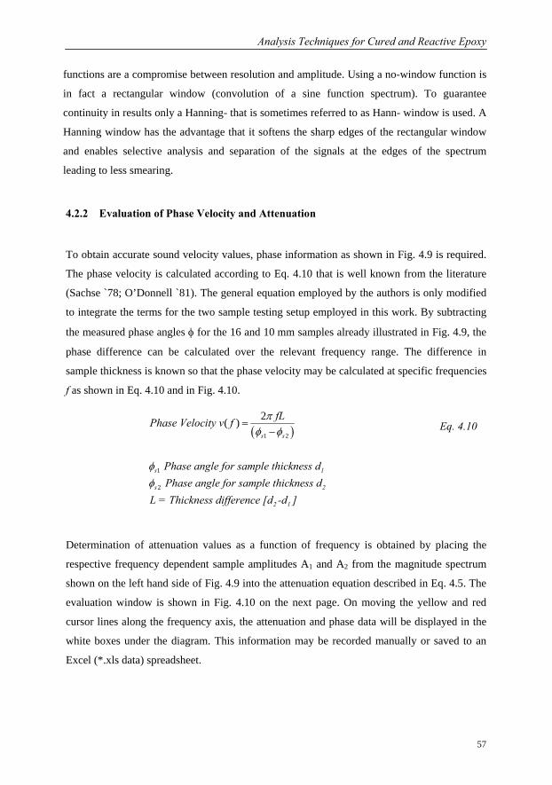
Analysis Techniques for Cured and Reactive Epoxy
57
( )1 2
1
2
2( )s s
s 1
s 2
2 1
fLPhase Velocity v f
Phase angle for sample thickness d Phase angle for sample thickness d
L = Thickness difference [d -d ]
πφ φ
φφ
=−
functions are a compromise between resolution and amplitude. Using a no-window function is
in fact a rectangular window (convolution of a sine function spectrum). To guarantee
continuity in results only a Hanning- that is sometimes referred to as Hann- window is used. A
Hanning window has the advantage that it softens the sharp edges of the rectangular window
and enables selective analysis and separation of the signals at the edges of the spectrum
leading to less smearing.
4.2.2 Evaluation of Phase Velocity and Attenuation
To obtain accurate sound velocity values, phase information as shown in Fig. 4.9 is required.
The phase velocity is calculated according to Eq. 4.10 that is well known from the literature
(Sachse `78; O’Donnell `81). The general equation employed by the authors is only modified
to integrate the terms for the two sample testing setup employed in this work. By subtracting
the measured phase angles φ for the 16 and 10 mm samples already illustrated in Fig. 4.9, the
phase difference can be calculated over the relevant frequency range. The difference in
sample thickness is known so that the phase velocity may be calculated at specific frequencies
f as shown in Eq. 4.10 and in Fig. 4.10.
Determination of attenuation values as a function of frequency is obtained by placing the
respective frequency dependent sample amplitudes A1 and A2 from the magnitude spectrum
shown on the left hand side of Fig. 4.9 into the attenuation equation described in Eq. 4.5. The
evaluation window is shown in Fig. 4.10 on the next page. On moving the yellow and red
cursor lines along the frequency axis, the attenuation and phase data will be displayed in the
white boxes under the diagram. This information may be recorded manually or saved to an
Excel (*.xls data) spreadsheet.
Eq. 4.10
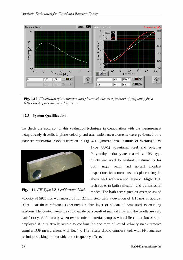
Analysis Techniques for Cured and Reactive Epoxy
58 BAM-Dissertationsreihe
Fig. 4.10: Illustration of attenuation and phase velocity as a function of frequency for a fully cured epoxy measured at 25 °C
.
4.2.3 System Qualification:
To check the accuracy of this evaluation technique in combination with the measurement
setup already described, phase velocity and attenuation measurements were performed on a
standard calibration block illustrated in Fig. 4.11 (International Institute of Welding: IIW
Type US-1) containing steel and polymer
Polymethylmethacrylate materials. IIW type
blocks are used to calibrate instruments for
both angle beam and normal incident
inspections. Measurements took place using the
above FFT software and Time of Flight TOF
techniques in both reflection and transmission
modes. For both techniques an average sound
velocity of 5920 m/s was measured for 22 mm steel with a deviation of ± 10 m/s or approx.
0.3 %. For these reference experiments a thin layer of silicon oil was used as coupling
medium. The quoted deviation could easily be a result of manual error and the results are very
satisfactory. Additionally when two identical material samples with different thicknesses are
employed it is relatively simple to confirm the accuracy of sound velocity measurements
using a TOF measurement with Eq. 4.7. The results should compare well with FFT analysis
techniques taking into consideration frequency effects.
Fig. 4.11: IIW Type US-1 calibration block
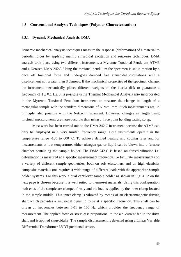
Analysis Techniques for Cured and Reactive Epoxy
59
4.3 Conventional Analysis Techniques (Polymer Characterisation)
4.3.1 Dynamic Mechanical Analysis, DMA
Dynamic mechanical analysis techniques measure the response (deformation) of a material to
periodic forces by applying mainly sinusoidal excitation and response techniques. DMA
analysis took place using two different instruments a Myrenne Torsional Pendulum ATM3
and a Netzsch DMA 242C. Using the torsional pendulum the specimen is set in motion by a
once off torsional force and undergoes damped free sinusoidal oscillations with a
displacement not greater than 3 degrees. If the mechanical properties of the specimen change,
the instrument mechanically places different weights on the inertia disk to guarantee a
frequency of 1 ± 0.1 Hz. It is possible using Thermal Mechanical Analysis also incorporated
in the Myrenne Torsional Pendulum instrument to measure the change in length of a
rectangular sample with the standard dimensions of 60*5*1 mm. Such measurements are, in
principle, also possible with the Netzsch instrument. However, changes in length using
torsional measurements are more accurate than using a three point bending testing setup.
Most work has been carried out on the DMA 242 C instrument because the ATM3 can
only be employed in a very limited frequency range. Both instruments operate in the
temperature range -150 to 600 °C. To achieve defined heating and cooling rates and for
measurements at low temperatures either nitrogen gas or liquid can be blown into a furnace
chamber containing the sample holder. The DMA 242 C is based on forced vibration i.e.
deformation is measured at a specific measurement frequency. To facilitate measurements on
a variety of different sample geometries, both on soft elastomers and on high elasticity
composite materials one requires a wide range of different loads with the appropriate sample
holder systems. For this work a dual cantilever sample holder as shown in Fig. 4.12 on the
next page is chosen because it is well suited to thermoset materials. Using this configuration
both ends of the sample are clamped firmly and the load is applied by the inner clamp located
in the sample middle. This inner clamp is vibrated by means of an electromagnetic driving
shaft which provides a sinusoidal dynamic force at a specific frequency. This shaft can be
driven at frequencies between 0.01 to 100 Hz which provides the frequency range of
measurement. The applied force or stress σ is proportional to the a.c. current fed to the drive
shaft and is applied sinusoidally. The sample displacement is detected using a Linear Variable
Differential Transformer LVDT positional sensor.
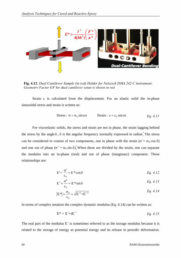
Analysis Techniques for Cured and Reactive Epoxy
60 BAM-Dissertationsreihe
Strain ε is calculated from the displacement. For an elastic solid the in-phase
sinusoidal stress and strain is written as:
For viscoelastic solids, the stress and strain are not in phase, the strain lagging behind
the stress by the angle δ , δ is the angular frequency normally expressed in radian The stress
can be considered to consist of two components, one in phase with the strain (σ´= σ0 cos δ)
and one out of phase (σ´´= σ0 sin δ). When these are divided by the strain, one can separate
the modulus into an in-phase (real) and out of phase (imaginary) component. These
relationships are:
In terms of complex notation the complex dynamic modulus (Eq. 4.14) can be written as:
The real part of the modulus E´ is sometimes referred to as the storage modulus because it is
related to the storage of energy as potential energy and its release in periodic deformation.
0 0Stress : sin t Strain : sin tσ = σ ω ε = ε ω
0
0
2 20
0
E´= E *cos
E´ E*sin
E* E´ +E´
′σ= δ
ε′′σ
= = δε
σ= =
ε
E* = E´+iE´´
Eq. 4.11
Eq. 4.12
Eq. 4.13
Eq. 4.14
Eq. 4.15
Fig. 4.12: Dual Cantilever Sample (in red) Holder for Netszsch DMA 242 C instrument: Geometry Factor GF for dual cantilever setup is shown in red
3
3
**4( ) *
l FEbh a
⎛ ⎞= ⎜ ⎟⎝ ⎠
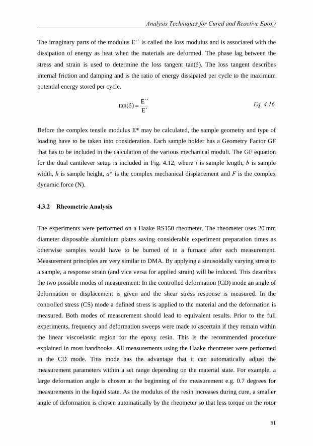
Analysis Techniques for Cured and Reactive Epoxy
61
The imaginary parts of the modulus E´´ is called the loss modulus and is associated with the
dissipation of energy as heat when the materials are deformed. The phase lag between the
stress and strain is used to determine the loss tangent tan(δ). The loss tangent describes
internal friction and damping and is the ratio of energy dissipated per cycle to the maximum
potential energy stored per cycle.
Before the complex tensile modulus E* may be calculated, the sample geometry and type of
loading have to be taken into consideration. Each sample holder has a Geometry Factor GF
that has to be included in the calculation of the various mechanical moduli. The GF equation
for the dual cantilever setup is included in Fig. 4.12, where l is sample length, b is sample
width, h is sample height, a* is the complex mechanical displacement and F is the complex
dynamic force (N).
4.3.2 Rheometric Analysis
The experiments were performed on a Haake RS150 rheometer. The rheometer uses 20 mm
diameter disposable aluminium plates saving considerable experiment preparation times as
otherwise samples would have to be burned of in a furnace after each measurement.
Measurement principles are very similar to DMA. By applying a sinusoidally varying stress to
a sample, a response strain (and vice versa for applied strain) will be induced. This describes
the two possible modes of measurement: In the controlled deformation (CD) mode an angle of
deformation or displacement is given and the shear stress response is measured. In the
controlled stress (CS) mode a defined stress is applied to the material and the deformation is
measured. Both modes of measurement should lead to equivalent results. Prior to the full
experiments, frequency and deformation sweeps were made to ascertain if they remain within
the linear viscoelastic region for the epoxy resin. This is the recommended procedure
explained in most handbooks. All measurements using the Haake rheometer were performed
in the CD mode. This mode has the advantage that it can automatically adjust the
measurement parameters within a set range depending on the material state. For example, a
large deformation angle is chosen at the beginning of the measurement e.g. 0.7 degrees for
measurements in the liquid state. As the modulus of the resin increases during cure, a smaller
angle of deformation is chosen automatically by the rheometer so that less torque on the rotor
E´tan( )E´
δ = Eq. 4.16
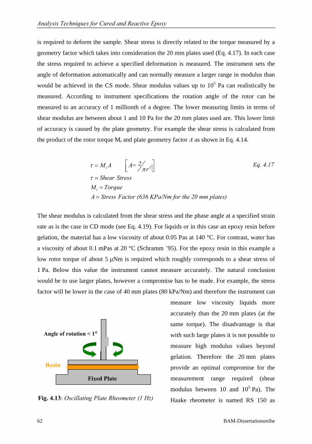
Analysis Techniques for Cured and Reactive Epoxy
62 BAM-Dissertationsreihe
is required to deform the sample. Shear stress is directly related to the torque measured by a
geometry factor which takes into consideration the 20 mm plates used (Eq. 4.17). In each case
the stress required to achieve a specified deformation is measured. The instrument sets the
angle of deformation automatically and can normally measure a larger range in modulus than
would be achieved in the CS mode. Shear modulus values up to 105 Pa can realistically be
measured. According to instrument specifications the rotation angle of the rotor can be
measured to an accuracy of 1 millionth of a degree. The lower measuring limits in terms of
shear modulus are between about 1 and 10 Pa for the 20 mm plates used are. This lower limit
of accuracy is caused by the plate geometry. For example the shear stress is calculated from
the product of the rotor torque Mt and plate geometry factor A as shown in Eq. 4.14.
The shear modulus is calculated from the shear stress and the phase angle at a specified strain
rate as is the case in CD mode (see Eq. 4.19). For liquids or in this case an epoxy resin before
gelation, the material has a low viscosity of about 0.05 Pas at 140 °C. For contrast, water has
a viscosity of about 0.1 mPas at 20 °C (Schramm `95). For the epoxy resin in this example a
low rotor torque of about 5 µNm is required which roughly corresponds to a shear stress of
1 Pa. Below this value the instrument cannot measure accurately. The natural conclusion
would be to use larger plates, however a compromise has to be made. For example, the stress
factor will be lower in the case of 40 mm plates (80 kPa/Nm) and therefore the instrument can
measure low viscosity liquids more
accurately than the 20 mm plates (at the
same torque). The disadvantage is that
with such large plates it is not possible to
measure high modulus values beyond
gelation. Therefore the 20 mm plates
provide an optimal compromise for the
measurement range required (shear
modulus between 10 and 105 Pa). The
Haake rheometer is named RS 150 as
3t
t
2M A A= rShear Stress
M TorqueA Stress Factor (636 KPa/Nm for the 20 mm plates)
τ πτ
⎡ ⎤= ⎢ ⎥⎣ ⎦=
==
Eq. 4.17
Resin
Angle of rotation < 1°
Fixed Plate
Fig. 4.13: Oscillating Plate Rheometer (1 Hz)
Analysis Techniques for Cured and Reactive Epoxy
63
150 mNm is the maximum torque at which the instrument can measure. The 20 mm
measurement plate diameter will not influence the determination of the gel point which
typically occurs at a viscosity of 10 kPas and is well within instrument measurement
tolerances. All experiments were conducted under isothermal conditions in the temperature
range between 60 and 100 °C. Before each measurement the parallel plate system was fully
closed and preheated to the isothermal temperature required. The instrument is then opened
and a few drops of resin are placed between the gap (see Fig. 4.12) and the measurement
starts when a gap of 0.5 mm is reached. Temperature is monitored by a thermocouple located
directly under the surface of the lower plate on which the resin is placed. Both the upper and
lower plates are electrically heated and an insulating ring is placed around the plates to
minimise heat loss. In the case of a pure solid the strain is directly related to the stress. The
strain response is said to be ‘In Phase’ and the phase angle δ = 0°. For a Newtonian liquid the
strain follows the stress at δ = 90°. In reality for an epoxy resin during cure the phase angle is
not constant and is between 0<δ<90°. In the controlled deformation mode, the deformation or
strain is described by the maximum amplitude or displacement γ0 and the angular velocity ω.
0 sin( )γ γ ω= ⋅ ⋅ t Eq. 4.18
The resulting shear stress is characterised by the amplitude of the stress and the phase angle δ.
0 sin( )τ τ ω δ= ⋅ ⋅ +t Eq. 4.19
The complex modulus G * and its parts G´ and G´´ are calculated as follows:
0
0
*G τγ
= Eq. 4.20
0
0
* ' '' τγ
= + =G G iG Eq.4.21
0
0
' * cos cosτδ δγ
= ⋅ =G G Eq. 4.22
0
0
* sin sinG G τδ δγ
′′ = ⋅ = ⋅ Eq. 4.23
For oscillatory shear measurements, the complex modulus and its parts are related to the
measured shear stress (Eqs. 4.18 to 4.23). The empirical Cox-Merz rule (Cox `58) states that
Analysis Techniques for Cured and Reactive Epoxy
64 BAM-Dissertationsreihe
the shear viscosity η should be the same function of shear rate as complex viscosity η * is of
frequency ω where:
2 21* '' G Gηω
′= + Eq. 4.24
and η ηω ω
′′ ′′ ′′= =
G G Eq. 4.25
The real or dynamic component η´ is often described as being related to the steady state or
shear viscosity and that it measures the rate of energy dissipation whereas the parameter η´´ is
related to the elastic or stored energy of the resin as described in Eq. 4.25. This is sometimes
confusing as one could easily assume that the steady state viscosity (typically measured in
rotation η) is equal to the dynamic viscosity η´. The measured viscosity for a steady shear
flow at low strain rates or velocity gradients is actually equal to the complex viscosity ⏐η*⏐
(as illustrated in Eq. 4.24) under the condition that small deformation angles or amplitudes are
employed for such experiments (Cox `58). This rule applies for liquids and not for relaxations
in polymers or viscoelastic materials i.e. ωτ<<1 (see Chapter 2.3.1). The deformation range in
which this rule may be applied is usually determined by varying the deformation amplitude as
function of measurement frequency. In the linear range this rule is generally accepted as being
valid in most scientific literature (Schramm `95).
4.3.3 Differential Scanning Calorimetry (DSC)
All experiments were conducted on a Netzsch DSC 204 F1 Phoenix instrument and take place
in the presence of nitrogen to avoid oxidation of the samples. The construction is based on the
heat flux principle. The instrument (Fig. 4.14) holds two identical pans: a sample pan with
about 10 mg of resin and a generally empty reference or neutral pan. The pans and lids are
composed of aluminium and are not airtight as it may lead to unwanted volume changes
between sample and reference. Heat flux is based on the transfer of heat to the sample and
reference being closely controlled while the instrument monitors the temperature difference
between the two pans. Experiments are performed both at constant temperature and also by
changing the temperature at various constant heating rates, called temperature scanning. As
long as the sample and the reference pan respond to the temperature program in the same way,
the heat flux remains nearly constant as does the temperature difference between the two
sensor plates located beneath the pans. If the sample absorbs heat because of melting or glass
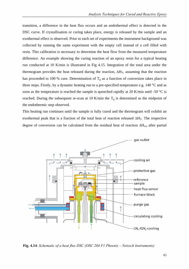
Analysis Techniques for Cured and Reactive Epoxy
65
transition, a difference in the heat flux occurs and an endothermal effect is detected in the
DSC curve. If crystallisation or curing takes place, energy is released by the sample and an
exothermal effect is observed. Prior to each set of experiments the instrument background was
collected by running the same experiment with the empty cell instead of a cell filled with
resin. This calibration is necessary to determine the heat flow from the measured temperature
difference. An example showing the curing reaction of an epoxy resin for a typical heating
run conducted at 10 K/min is illustrated in Fig 4.15. Integration of the total area under the
thermogram provides the heat released during the reaction, ΔHT, assuming that the reaction
has proceeded to 100 % cure. Determination of Tg as a function of conversion takes place in
three steps. Firstly, by a dynamic heating run to a pre-specified temperature e.g. 140 °C and as
soon as the temperature is reached the sample is quenched rapidly at 20 K/min until -50 °C is
reached. During the subsequent re-scan at 10 K/min the Tg is determined as the midpoint of
the endothermic step observed.
This heating run continues until the sample is fully cured and the thermogram will exhibit an
exothermal peak that is a fraction of the total heat of reaction released ΔHT. The respective
degree of conversion can be calculated from the residual heat of reaction ΔHres after partial
Fig. 4.14: Schematic of a heat flux DSC (DSC 204 F1 Phoenix – Netzsch Instruments)
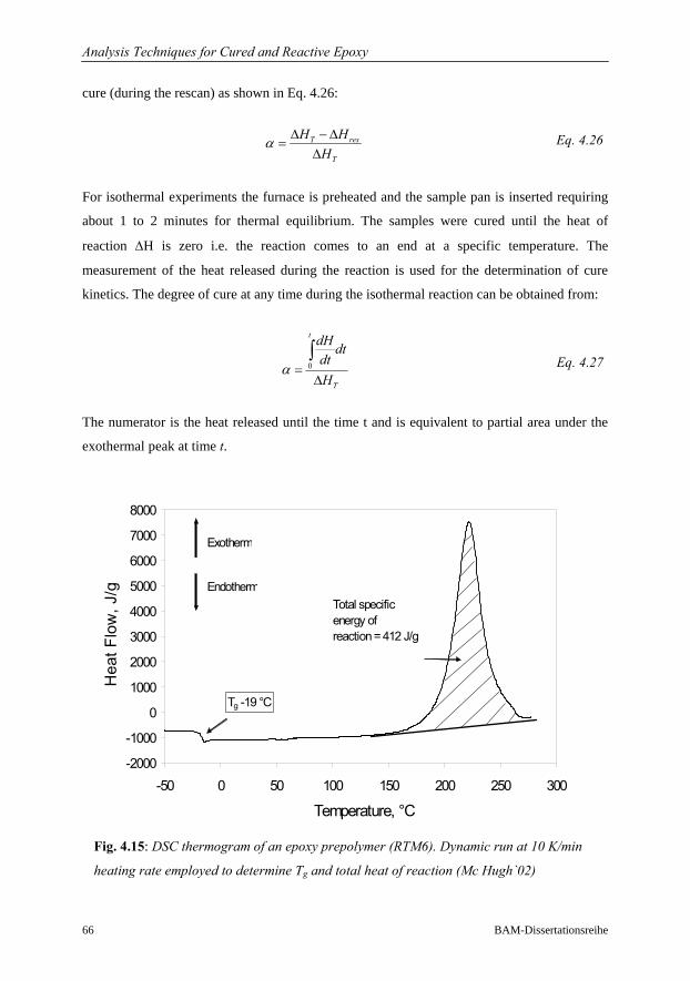
Analysis Techniques for Cured and Reactive Epoxy
66 BAM-Dissertationsreihe
cure (during the rescan) as shown in Eq. 4.26:
For isothermal experiments the furnace is preheated and the sample pan is inserted requiring
about 1 to 2 minutes for thermal equilibrium. The samples were cured until the heat of
reaction ΔH is zero i.e. the reaction comes to an end at a specific temperature. The
measurement of the heat released during the reaction is used for the determination of cure
kinetics. The degree of cure at any time during the isothermal reaction can be obtained from:
The numerator is the heat released until the time t and is equivalent to partial area under the
exothermal peak at time t.
-2000
-1000
0
1000
2000
3000
4000
5000
6000
7000
8000
-50 0 50 100 150 200 250 300
Temperature, °C
Hea
t Flo
w, J
/g
Tg -19 °C
Total specific energy of reaction = 412 J/g
Exotherm
Endotherm
Fig. 4.15: DSC thermogram of an epoxy prepolymer (RTM6). Dynamic run at 10 K/min
heating rate employed to determine Tg and total heat of reaction (Mc Hugh`02)
Eq. 4.26
Eq. 4.27
T res
T
H HH
α Δ − Δ=
Δ
0=Δ
∫t
T
dH dtdtH
α
Analysis Techniques for Cured and Reactive Epoxy
67
4.4 Epoxy-Amine System
Only one epoxy resin system is employed throughout this thesis. It is a commercial epoxy
laminating epoxy resin with the trade name L335 from the company Martin G. Scheuffler
(now part of the Hexion Group). The resin system is approved by the German Federal
Aviation Authority and it is mainly employed in the production of light airplanes, gliders and
boots. It is also employed as a laminating resin in combination with either glass or carbon
fibre. It has a pot life at room temperature that depending on mixing ratio ranges between
10 mins and 6 to 7 h. It is most commonly used in combination with an amine based hardener
systems referred to as H335 or H340. The resin system employed here is a combination of
L385:H340 in the mixing ratio of 100:38 parts per weight. At room temperature cure times of
between 24 and 30 h requiring about 4 h to gel (defined as time to reach a viscosity of
5000 mPas) are recommended. The viscosity value of 5000 mPas is an arbitrary value
normally provided on manufacturer’s data sheets. For viscosity values higher than 5000 mPas
it becomes increasingly difficult to achieve mould filling and fibre impregnation. The amine
hardener referred to by the number H340 has a light blue colour. Both components
L335:H340 are mixed until a homogene blue colour is obtained for the mixture. All mixing
takes place at room temperature independent of the experimental routine or heating regime
following. The cured epoxy has a light blue transparent colour and according to its data sheet
has a glass transition temperature of approx. 75 °C for the fully cured resin system. No
information is provided on how this value is obtained and it is presumed that it is determined
by the peak maximum in the loss modulus for DMA techniques at low frequency, which is
common for material data sheets. The epoxy system has a density of 1.18 to 1.2 g/cm³.
Viscosity of the epoxy is listed on the data sheet as between 2300 to 2900 mPas and the
hardener has a viscosity of 170 to 190 mPas both measured individually at room temperature.
68 BAM-Dissertationsreihe
Chapter 5
5 Experimental Results
Remarks on Layout of Experimental Results
Experimental results are split into three sections: Chapter 5.1 is concerned with principle
questions relating to the suitability of acoustic measurements for accurate analysis of dynamic
mechanical thermal properties of a non-reactive fully cured epoxy*. Factors such as
interpretation of longitudinal L´ and shear G´ storage moduli as determined from wave
propagation experiments as well as the influence of measurement frequency are considered
and the results are compared with conventional DMA. A detailed breakdown of objectives is
provided on the next page.
In Chapter 5.2 starting on page 87 the two sample technique already presented is
adapted for cure monitoring experiments. The crosslinking reaction for epoxy polymers is
exothermic and the thicker the sample the more heat will be given off. If a two sample
technique with varying sample thickness were used it would be difficult to maintain or
guarantee constant temperatures for both samples. However, constant temperatures are
essential for comparison of all cure monitoring experiments using different analysis
techniques. In Chapter 5.2 the adaptation as well as accuracy, limitations and advantages of a
new single sample technique are discussed using experimental results.
In Chapter 5.3 the sensitivity of a single sample technique to variations in the
viscoelastic properties resulting from the curing reaction of an epoxy is evaluated. The
measured ultrasound parameters are compared with conventional analysis techniques
typically used to characterise chemorheological cure properties i.e. changes in viscoelastic
properties as a result of the curing reaction. More detailed explanations and breakdown of
objectives and procedures are provided in Chapter 5.3.1 and starting on page 88.
* Only one epoxy is used for all experiments (see Chapter 4.4)
Experimental Results
69
5.1 Investigations on a Cured Epoxy
A breakdown of the objectives for experiments on cured epoxy is provided in the following.
As it is difficult to maintain an overview, the results are divided under three sub-headings. All
experiments take place in the dynamic temperature range between 20 and 200 °C.
1. The mechanical behaviour of an epoxy is analysed using conventional DMA in the
frequency range 0.1 to 50 Hz. From the results the parameters for the Williams Landel
Ferry WLF relation can be determined using Time Temperature Superposition
principles and employed to predict the influence of measurement frequency on
experimental results up to MHz range. This information provides a means of
predicting and interpreting results at ultrasound measurement frequencies.
2. Interpretation of the measured ultrasound parameters sound velocity and attenuation as
a function of temperature are considered. This takes into account the influence of
dispersion and attenuation on measured results. Secondly, the measured ultrasound
parameters are converted into longitudinal storage L´ modulus and tan(δ). Reduced
equations (Eqs. 2.9 to 2.16) are validated by showing that the term αλ/2π <<1 and
may be used to evaluate L´ and G´. Using a two sample technique quantitative values
for attenuation can be determined and the influence of high attenuation α values at Tg
on the accuracy of the calculated modulus L´ and tan(δ) can be discussed. Lastly
the influence of measurement frequency is discussed and the α relaxation is shown to
obey a WLF-temperature dependence.
3. The longitudinal L´ and shear G´ storage moduli are measured using wave propagation
techniques as a function of temperature. By measuring any two storage moduli, it is
possible to evaluate any other modulus term or Poisson’s ratio μp´ (see Chapter 2.2.3).
Because shear waves do not propagate in soft polymers it was only possible to
estimate G´ in the soft polymer by extrapolating μp´ to known values for rubbers. In
this manner, the respective bulk K´ and tensile E´ storage moduli could be determined
over a large temperature range and for an α relaxation process. This provides the
opportunity to study the interrelationship of the various moduli and to investigate the
sensitivity or limitations of longitudinal modulus L´, in contrast to for example other
more commonly used moduli such as G´ or E´.
Experimental Results
70 BAM-Dissertationsreihe
5.1.1 DMA in the Frequency Range between 0.1 to 50 Hz
Fig. 5.1 illustrates the tensile storage E´ modulus and tan(δ) as a function of temperature at
specific frequencies between 0.1 and 50 Hz. Measurements were performed using the DMA
242 C instrument (Chapter 4.3) and a dual cantilever setup. Straight lines and symbols are
employed only to differentiate between the curves and should not be mistaken for
measurement points. All curves are smoothed automatically with Netzsch instrument software
and the data is saved as ASCII file. From the elastic modulus values, three distinct regions can
be identified in the 25 to 200 °C temperature range. At low temperatures, the polymer is stiff
or frozen with an accordingly high modulus and low tan(δ). As the temperature increases, the
polymer softens and in the third region (>100°C) the material behaves like a soft rubber and
has a low modulus. This transition from a hard stiff polymer to a rubber-like polymer and the
associated loss peak is referred to as glass transition Tg or α relaxation depending on
relevance (see Chapter 2.3.1). In analogy with this process a drop in modulus occurs and the
loss factor tan(δ) forms a peak. For reference purposes this transition region is typically
described by one specific temperature referred to as Tg and taken as the peak maximum
temperature of tan(δ). A shift in the tan(δ) maximum from 82°C at 0.1 Hz to 98°C at 50 Hz is
observed, which is an apparent shift of 16 K over 2.5 decades in frequency or approx. 6.5 K
per decade change in frequency. This is close to a general rule of thumb stating that the α
relaxation will be observed at 7 K higher temperatures for every decade increase in frequency
(Sperling `92; Cowie `91). As discussed in Chapter 2.3.2 this rule assumes a linear
relationship between frequency and the reciprocal of temperature, commonly illustrated by an
Arrhenius plot. Although some exceptions exist, an Arrhenius plot of α relaxation
temperature values versus frequency will typically form a curve (Aklonis `72). In such cases
the Williams Landel Ferry (WLF) equation (Eq. 2.28) is more suitable to describe frequency
behaviour. Values for WLF parameters may be obtained using Time Temperature
Superposition (TTS) principles. Rather than presenting temperature dependent measurements
at specific frequencies, the same mechanical modulus or loss factor may be plotted as a
function of frequency at constant temperature. A master curve may be formed by shifting
these partial isothermal temperature curves to form a smooth composite curve (Fig. 5.2). On
constructing this master curve the time-dependent modulus obtained at 80 °C was used as
reference (full circles), while all other curves were horizontally displaced along the
logarithmic frequency axis by a shift factor denoted as aT.
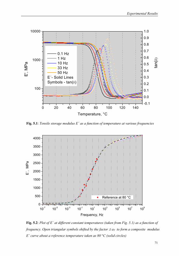
Experimental Results
71
0 20 40 60 80 100 120 140
100
1000
10000
-0.1
0.0
0.1
0.2
0.3
0.4
0.5
0.6
0.7
0.8
0.9
1.0
0.1 Hz 1 Hz 10 Hz 33 Hz 50 Hz
E´- Solid LinesSymbols - tan(δ)
tan(
δ)
E',
MPa
Temperature, °C
Fig. 5.1: Tensile storage modulus E´ as a function of temperature at various frequencies
10-7 10-5 10-3 10-1 101 103 105 107 1090
500
1000
1500
2000
2500
3000
3500
4000
Reference at 80 °C
E´,
MP
a
Frequency, Hz
Fig. 5.2: Plot of E´ at different constant temperatures (taken from Fig. 5.1) as a function of
frequency. Open triangular symbols shifted by the factor ± aT to form a composite modulus
E´ curve about a reference temperature taken as 80 °C (solid circles)
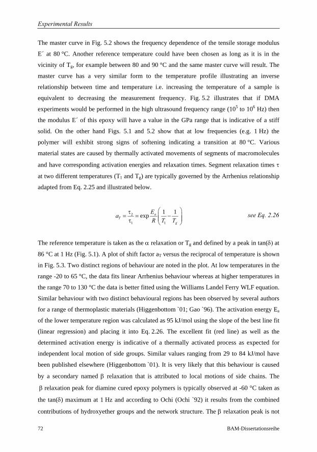
Experimental Results
72 BAM-Dissertationsreihe
The master curve in Fig. 5.2 shows the frequency dependence of the tensile storage modulus
E´ at 80 °C. Another reference temperature could have been chosen as long as it is in the
vicinity of Tg, for example between 80 and 90 °C and the same master curve will result. The
master curve has a very similar form to the temperature profile illustrating an inverse
relationship between time and temperature i.e. increasing the temperature of a sample is
equivalent to decreasing the measurement frequency. Fig. 5.2 illustrates that if DMA
experiments would be performed in the high ultrasound frequency range (105 to 106 Hz) then
the modulus E´ of this epoxy will have a value in the GPa range that is indicative of a stiff
solid. On the other hand Figs. 5.1 and 5.2 show that at low frequencies (e.g. 1 Hz) the
polymer will exhibit strong signs of softening indicating a transition at 80 °C. Various
material states are caused by thermally activated movements of segments of macromolecules
and have corresponding activation energies and relaxation times. Segment relaxation times τ
at two different temperatures (T1 and Tg) are typically governed by the Arrhenius relationship
adapted from Eq. 2.25 and illustrated below.
The reference temperature is taken as the α relaxation or Tg and defined by a peak in tan(δ) at
86 °C at 1 Hz (Fig. 5.1). A plot of shift factor aT versus the reciprocal of temperature is shown
in Fig. 5.3. Two distinct regions of behaviour are noted in the plot. At low temperatures in the
range -20 to 65 °C, the data fits linear Arrhenius behaviour whereas at higher temperatures in
the range 70 to 130 °C the data is better fitted using the Williams Landel Ferry WLF equation.
Similar behaviour with two distinct behavioural regions has been observed by several authors
for a range of thermoplastic materials (Higgenbottom `01; Gao `96). The activation energy Ea
of the lower temperature region was calculated as 95 kJ/mol using the slope of the best line fit
(linear regression) and placing it into Eq. 2.26. The excellent fit (red line) as well as the
determined activation energy is indicative of a thermally activated process as expected for
independent local motion of side groups. Similar values ranging from 29 to 84 kJ/mol have
been published elsewhere (Higgenbottom `01). It is very likely that this behaviour is caused
by a secondary named β relaxation that is attributed to local motions of side chains. The
β relaxation peak for diamine cured epoxy polymers is typically observed at -60 °C taken as
the tan(δ) maximum at 1 Hz and according to Ochi (Ochi `92) it results from the combined
contributions of hydroxyether groups and the network structure. The β relaxation peak is not
2
1 1
1 1exp ⎛ ⎞τ
= = −⎜ ⎟⎜ ⎟τ ⎝ ⎠
aT
g
EaR T T
see Eq. 2.26
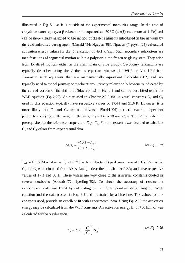
Experimental Results
73
illustrated in Fig. 5.1 as it is outside of the experimental measuring range. In the case of
anhydride cured epoxy, a β relaxation is expected at -70 °C (tan(δ) maximum at 1 Hz) and
can be more clearly assigned to the motion of diester segments introduced in the network by
the acid anhydride curing agent (Masaki `84; Nguyen `95). Nguyen (Nguyen `95) calculated
activation energy values for the β relaxation of 49.1 kJ/mol. Such secondary relaxations are
manifestations of segmental motion within a polymer in the frozen or glassy state. They arise
from localised motions either in the main chain or side groups. Secondary relaxations are
typically described using the Arrhenius equation whereas the WLF or Vogel-Fulcher-
Tammann VFT equations that are mathematically equivalent (Schönhals `02) and are
typically used to model primary or α relaxations. Primary relaxation behaviour is indicated by
the curved portion of the shift plot (blue points) in Fig. 5.3 and can be best fitted using the
WLF equation (Eq. 2.29). As discussed in Chapter 2.3.2 the universal constants C1 and C2
used in this equation typically have respective values of 17.44 and 51.6 K. However, it is
more likely that C1 and C2 are not universal (Strobl `96) but are material dependent
parameters varying in the range in the range C1 = 14 to 18 and C2 = 30 to 70 K under the
prerequisite that the reference temperature Tref = Tg. For this reason it was decided to calculate
C1 and C2 values from experimental data.
1
2
( )log ref
Tref
C T Ta
C T T− −
=+ −
Tref in Eq. 2.29 is taken as Tg = 86 °C i.e. from the tan(δ) peak maximum at 1 Hz. Values for
C1 and C2 were obtained from DMA data (as described in Chapter 2.2.3) and have respective
values of 17.3 and 56 K. These values are very close to the universal constants quoted in
several textbooks (Aklonis `72; Sperling `92). To check the accuracy of results the
experimental data was fitted by calculating aT in 5 K temperature steps using the WLF
equation and the data plotted in Fig. 5.3 and illustrated by a blue line. The values for the
constants used, provide an excellent fit with experimental data. Using Eq. 2.30 the activation
energy may be calculated from the WLF constants. An activation energy Ea of 760 kJ/mol was
calculated for the α relaxation.
see Eq. 2.29
21
2
2.303 ⎛ ⎞
= ⎜ ⎟⎝ ⎠
a gCE RTC
see Eq. 2.30
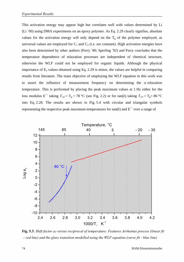
Experimental Results
74 BAM-Dissertationsreihe
This activation energy may appear high but correlates well with values determined by Li
(Li `00) using DMA experiments on an epoxy polymer. As Eq. 2.29 clearly signifies, absolute
values for the activation energy will only depend on the Tg of the polymer employed, as
universal values are employed for C1 and C2 (i.e. are constant). High activation energies have
also been determined by other authors (Ferry `80; Sperling `92) and Ferry concludes that the
temperature dependence of relaxation processes are independent of chemical structure,
otherwise the WLF could not be employed for organic liquids. Although the physical
importance of Ea values obtained using Eq. 2.29 is minor, the values are helpful in comparing
results from literature. The main objective of employing the WLF equation in this work was
to assert the influence of measurement frequency on determining the α relaxation
temperature. This is performed by placing the peak maximum values at 1 Hz either for the
loss modulus E´´ taking Tref = Tg = 78 °C (see Fig. 2.2) or for tan(δ) taking Tref = Tg= 86 °C
into Eq. 2.28. The results are shown in Fig. 5.4 with circular and triangular symbols
representing the respective peak maximum temperatures for tan(δ) and E´´ over a range of
2.4 2.6 2.8 3.0 3.2 3.4 3.6 3.8 4.0 4.2-10
-8
-6
-4
-2
0
2
4
6
8
10
12- 35
Temperature, °C145 540 85 - 20
80 °C
Log
a T
1000/T, K-1
Fig. 5.3: Shift factor aT versus reciprocal of temperature. Features Arrhenius process (linear fit
– red line) and the glass transition modelled using the WLF equation (curve fit - blue line)
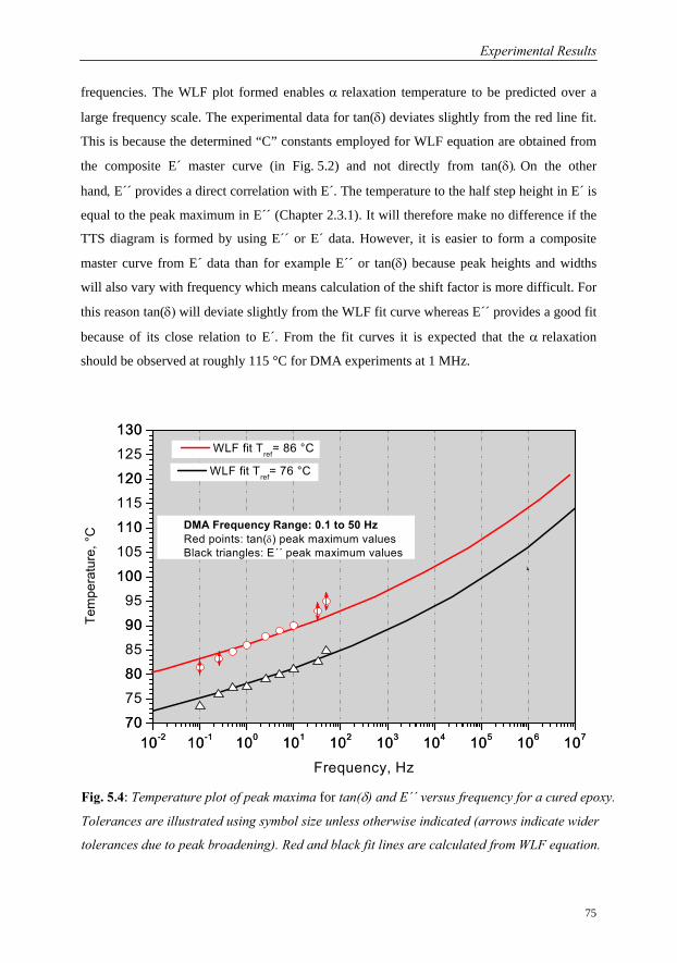
Experimental Results
75
frequencies. The WLF plot formed enables α relaxation temperature to be predicted over a
large frequency scale. The experimental data for tan(δ) deviates slightly from the red line fit.
This is because the determined “C” constants employed for WLF equation are obtained from
the composite E´ master curve (in Fig. 5.2) and not directly from tan(δ). On the other
hand, E´´ provides a direct correlation with E´. The temperature to the half step height in E´ is
equal to the peak maximum in E´´ (Chapter 2.3.1). It will therefore make no difference if the
TTS diagram is formed by using E´´ or E´ data. However, it is easier to form a composite
master curve from E´ data than for example E´´ or tan(δ) because peak heights and widths
will also vary with frequency which means calculation of the shift factor is more difficult. For
this reason tan(δ) will deviate slightly from the WLF fit curve whereas E´´ provides a good fit
because of its close relation to E´. From the fit curves it is expected that the α relaxation
should be observed at roughly 115 °C for DMA experiments at 1 MHz.
10-2 10-1 100 101 102 103 104 105 106 10770
75
80
85
90
95
100
105
110
115
120
125
130
10-2 10-1 100 101 102 103 104 105 106 10770
80
90
100
110
120
130
Tem
pera
ture
, °C
Frequency, Hz
WLF fit Tref= 86 °C
DMA Frequency Range: 0.1 to 50 HzRed points: tan(δ) peak maximum valuesBlack triangles: E´´ peak maximum values
WLF fit Tref= 76 °C
Fig. 5.4: Temperature plot of peak maxima for tan(δ) and E´´ versus frequency for a cured epoxy.
Tolerances are illustrated using symbol size unless otherwise indicated (arrows indicate wider
tolerances due to peak broadening). Red and black fit lines are calculated from WLF equation.
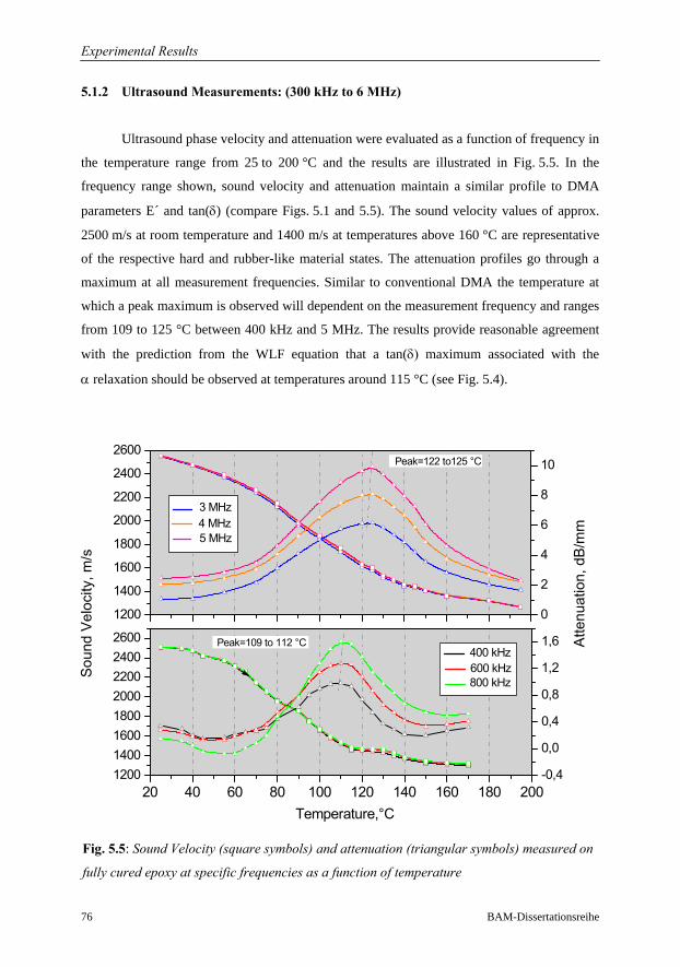
Experimental Results
76 BAM-Dissertationsreihe
5.1.2 Ultrasound Measurements: (300 kHz to 6 MHz)
Ultrasound phase velocity and attenuation were evaluated as a function of frequency in
the temperature range from 25 to 200 °C and the results are illustrated in Fig. 5.5. In the
frequency range shown, sound velocity and attenuation maintain a similar profile to DMA
parameters E´ and tan(δ) (compare Figs. 5.1 and 5.5). The sound velocity values of approx.
2500 m/s at room temperature and 1400 m/s at temperatures above 160 °C are representative
of the respective hard and rubber-like material states. The attenuation profiles go through a
maximum at all measurement frequencies. Similar to conventional DMA the temperature at
which a peak maximum is observed will dependent on the measurement frequency and ranges
from 109 to 125 °C between 400 kHz and 5 MHz. The results provide reasonable agreement
with the prediction from the WLF equation that a tan(δ) maximum associated with the
α relaxation should be observed at temperatures around 115 °C (see Fig. 5.4).
Fig. 5.5: Sound Velocity (square symbols) and attenuation (triangular symbols) measured on
fully cured epoxy at specific frequencies as a function of temperature
1200
1400
1600
1800
2000
2200
2400
2600
0
2
4
6
8
10
20 40 60 80 100 120 140 160 180 20012001400160018002000220024002600
-0,4
0,0
0,4
0,8
1,2
1,6
4 MHz4 MHz
Atte
nuat
ion,
dB
/mm
Peak=109 to 112 °C
Peak=122 to125 °C
Sou
nd V
eloc
ity, m
/s
3 MHz4 MHz 5 MHz
Temperature,°C
600 kHz800 kHz
400 kHz
Experimental Results
77
Combining this information with the interpretation of the temperature profile of the
corresponding sound velocity data it is supposed that the attenuation peak and large change in
sound velocity occurring in the 90 to 130 °C range are caused by a the α relaxation. This is
easily confirmed by calculating the parameters tan(δ) and L´ and placing the information into
the WLF equation as will be demonstrated later in this chapter. At present it is worth
discussing some other interesting effects, in particular regarding the attenuation profile and
measured values obtained. Firstly, the intensity of the attenuation peak is frequency
dependent, clearly increasing with increasing frequency. This behaviour is well known and is
also observed in conventional DMA when the behaviour of the loss modulus E´´ and not
tan(δ) is considered. For the α relaxation process, the peak intensity of the loss factor is
directly related to the co-ordinated chain molecular friction, which dissipates mechanical
energy as heat (Ding `06). Therefore at higher frequencies energy dissipation is larger and
accordingly the intensity of attenuation. However, an effect that is not well understood is the
frequency dependence of attenuation intensity at lower temperatures or well above or below
the primary α relaxation process. For example, if attenuation is plotted as a function of
frequency at 40 °C a linear dependence is observed as illustrated in Fig. 5.6. According to the
literature this attenuation behaviour is typical for polymers either with amorphous or
crystalline structures (McIntire `91; Hartmann `72). Hartman (Hartman `72, `94) compared
some of the more common acoustic models with experimental results (on PMMA and PE
thermoplastic polymers) but came to no satisfactory conclusion that would provide a physical
explanation for this behaviour. He also concluded, from experimental data, that this effect is
not caused by relaxation behaviour or as Ferry (Ferry `80) suggested by a broad distribution
of relaxation times. It is most likely caused by anelastic behaviour i.e. time dependence of the
stress strain response of polymers outside regions of molecular relaxation. If the stress strain
curve for a single cycle of vibrations is in the form of a hysteresis loop, then the area enclosed
under the loop will represent the mechanical energy that has been lost as heat (Kolsky `63). It
is known that hysteresis losses due to absorption αh in polymers should follow a linear
frequency dependence, where Ch is a constant and the notation h refers to hysteresis
(McIntire `91):
h h=C fα
As the wavelength is inversely proportional to frequency at constant sound velocity then
hysteresis absorption is one for which: .constαλ = The effect of this type of hysteresis is that
the energy loss per cycle will be constant so that the actual intensity of αλ will be
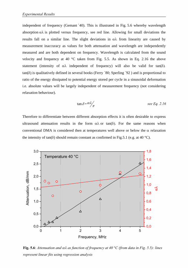
Experimental Results
78 BAM-Dissertationsreihe
independent of frequency (Gemant `40). This is illustrated in Fig. 5.6 whereby wavelength
absorption αλ is plotted versus frequency, see red line. Allowing for small deviations the
results fall on a similar line. The slight deviations in αλ from linearity are caused by
measurement inaccuracy as values for both attenuation and wavelength are independently
measured and are both dependent on frequency. Wavelength is calculated from the sound
velocity and frequency at 40 °C taken from Fig. 5.5. As shown in Eq. 2.16 the above
statement (intensity of αλ independent of frequency) will also be valid for tan(δ).
tan(δ) is qualitatively defined in several books (Ferry `80; Sperling `92 ) and is proportional to
ratio of the energy dissipated to potential energy stored per cycle in a sinusoidal deformation
i.e. absolute values will be largely independent of measurement frequency (not considering
relaxation behaviour).
Therefore to differentiate between different absorption effects it is often desirable to express
ultrasound attenuation results in the form αλ or tan(δ). For the same reasons when
conventional DMA is considered then at temperatures well above or below the α relaxation
the intensity of tan(δ) should remain constant as confirmed in Fig.5.1 (e.g. at 40 °C).
see Eq. 2.16 tan =αλδ π
Fig. 5.6: Attenuation and αλ as function of frequency at 40 °C (from data in Fig. 5.5): lines
represent linear fits using regression analysis
0 1 2 3 4 50,0
0,5
1,0
1,5
2,0
2,5
3,0
0,0
0,2
0,4
0,6
0,8
1,0
1,2
1,4
1,6
1,8α
λ
Atte
nuat
ion,
dB
/mm
Frequency, MHz
Temperature 40 °C
Experimental Results
79
5.1.3 Comparison of Ultrasound Results with Conventional DMA
To compare ultrasound with the results from conventional DMA, sound velocity and
attenuation need to be converted into corresponding modulus terms L´ and L´´ and tan(δ). As
shown in Eqs. 2.9 to 2.12 the calculation of tan(δ) and the longitudinal moduli L´ and L´´ can
be greatly simplified if the term αλ/ω shown in Eq. 2.13 has a value much less than unity. As
accurate values for both α and λ as functions of frequency are available from the experiments,
it can be demonstrated that αλ/ω<<1 is valid even for peak maximum values occurring at
α relaxation. Maximum attenuation values (Fig. 5.5) are taken as 8 dB/mm at 4 MHz and a
correlating wavelength λ of 0.54 mm (2160 m/s). The attenuation term α employed in the
wave equation to derive the complex modulus in Chapter 2.2.3 is measured in Neper whereas
results presented in this work use decibel dB units, which are more common for acoustic
applications. To convert from dB to Neper a multiplication factor of 8.686 is employed (see
Eq. 2.13).
With this knowledge the following reduced equations are valid for longitudinal modulus L´
and loss L´´ taking αλ/ω <<1 .
Before L´ and L´´ can be calculated the change in density ρ as a function of temperature is
required. Firstly ρ is measured at room temperature using Archimedes principles according to
DIN 53479. Using Thermal Mechanical Analysis TMA (Chapter 4.3) the change in sample
length for a rectangular sample can be measured experimentally over the temperature range
from -20 to 160 °C and the results are shown in Fig. 5.7. When the change of length is known
then the resulting change in volume V for a sample of known geometry can be calculated.
Mass m is taken as constant and the density change over the temperature range can be easily
calculated from using m/ΔV. Density only changes by about 4 % in the relevant temperature
range from 20 to 160 °C. All necessary parameters have been determined making it possible
to determine L´; L´´ and tan(δ) as function of temperature.
32 and ′ ′′= = cL c L ρ αρ ω
see Eqs. 2.9 to 2.12
108.0)686.8(2
)54.0(82
c<<=
π=
παλ
=ω
α
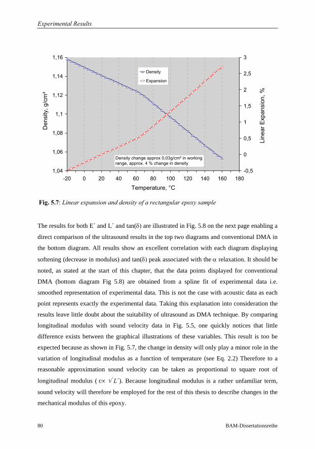
Experimental Results
80 BAM-Dissertationsreihe
The results for both E´ and L´ and tan(δ) are illustrated in Fig. 5.8 on the next page enabling a
direct comparison of the ultrasound results in the top two diagrams and conventional DMA in
the bottom diagram. All results show an excellent correlation with each diagram displaying
softening (decrease in modulus) and tan(δ) peak associated with the α relaxation. It should be
noted, as stated at the start of this chapter, that the data points displayed for conventional
DMA (bottom diagram Fig 5.8) are obtained from a spline fit of experimental data i.e.
smoothed representation of experimental data. This is not the case with acoustic data as each
point represents exactly the experimental data. Taking this explanation into consideration the
results leave little doubt about the suitability of ultrasound as DMA technique. By comparing
longitudinal modulus with sound velocity data in Fig. 5.5, one quickly notices that little
difference exists between the graphical illustrations of these variables. This result is too be
expected because as shown in Fig. 5.7, the change in density will only play a minor role in the
variation of longitudinal modulus as a function of temperature (see Eq. 2.2) Therefore to a
reasonable approximation sound velocity can be taken as proportional to square root of
longitudinal modulus ( c∝ √ L´). Because longitudinal modulus is a rather unfamiliar term,
sound velocity will therefore be employed for the rest of this thesis to describe changes in the
mechanical modulus of this epoxy.
Fig. 5.7: Linear expansion and density of a rectangular epoxy sample
1,04
1,06
1,08
1,1
1,12
1,14
1,16
-20 0 20 40 60 80 100 120 140 160 180
Temperature, °C
Den
sity
, g/c
m³
-0,5
0
0,5
1
1,5
2
2,5
3
Line
ar E
xpan
sion
, %
Density
Expansion
Density change approx 0,03g/cm² in working range, approx. 4 % change in density
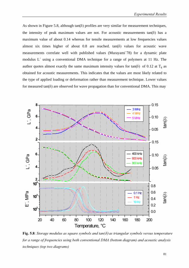
Experimental Results
81
As shown in Figure 5.8, although tan(δ) profiles are very similar for measurement techniques,
the intensity of peak maximum values are not. For acoustic measurements tan(δ) has a
maximum value of about 0.14 whereas for tensile measurements at low frequencies values
almost six times higher of about 0.8 are reached. tan(δ) values for acoustic wave
measurements correlate well with published values (Murayami`78) for a dynamic plate
modulus L´ using a conventional DMA technique for a range of polymers at 11 Hz. The
author quotes almost exactly the same maximum intensity values for tan(δ) of 0.12 at Tg as
obtained for acoustic measurements. This indicates that the values are most likely related to
the type of applied loading or deformation rather than measurement technique. Lower values
for measured tan(δ) are observed for wave propagation than for conventional DMA. This may
Fig. 5.8: Storage modulus as square symbols and tan(δ) as triangular symbols versus temperature
for a range of frequencies using both conventional DMA (bottom diagram) and acoustic analysis
techniques (top two diagrams)
2
4
6
8
0.05
0.10
0.15
2
4
6
8
0.00
0.05
0.10
0.15
20 40 60 80 100 120 140 160 180 200
102
103
104
0.0
0.2
0.4
0.6
0.8
3 MHz4 MHz5 MHz
E´, M
PaL´
, GP
aL´
, GPa
400 kHz600 kHz800 kHz
ta
n(δ)
tan(
δ)ta
n(δ)
Temperature, °C
0.1 Hz1 Hz10 Hz
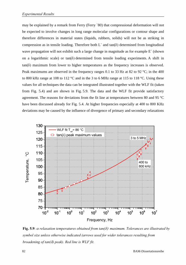
Experimental Results
82 BAM-Dissertationsreihe
may be explained by a remark from Ferry (Ferry `80) that compressional deformation will not
be expected to involve changes in long range molecular configurations or contour shape and
therefore differences in material states (liquids, rubbers, solids) will not be as striking in
compression as in tensile loading. Therefore both L´ and tan(δ) determined from longitudinal
wave propagation will not exhibit such a large change in magnitude as for example E´ (shown
on a logarithmic scale) or tan(δ) determined from tensile loading experiments. A shift in
tan(δ) maximum from lower to higher temperatures as the frequency increases is observed.
Peak maximums are observed in the frequency ranges 0.1 to 33 Hz at 82 to 92 °C; in the 400
to 800 kHz range at 108 to 112 °C and in the 3 to 6 MHz range at 115 to 118 °C. Using these
values for all techniques the data can be integrated illustrated together with the WLF fit (taken
from Fig. 5.4) and are shown in Fig. 5.9. The data and the WLF fit provide satisfactory
agreement. The reasons for deviations from the fit line at temperatures between 80 and 95 °C
have been discussed already for Fig. 5.4. At higher frequencies especially at 400 to 800 KHz
deviations may be caused by the influence of divergence of primary and secondary relaxations
Fig. 5.9: α relaxation temperatures obtained from tan(δ) maximum. Tolerances are illustrated by
symbol size unless otherwise indicated (arrows used for wider tolerances resulting from
broadening of tan(δ) peak). Red line is WLF fit.
10-2 10-1 100 101 102 103 104 105 106 10770
75
80
85
90
95
100
105
110
115
120
125
130
10-2 10-1 100 101 102 103 104 105 106 10770
80
90
100
110
120
130
3 to 5 MHz
400 to 800 kHz
Tem
pera
ture
, °C
Frequency, Hz
WLF fit Tref= 86 °C tan(δ) peak maximum values
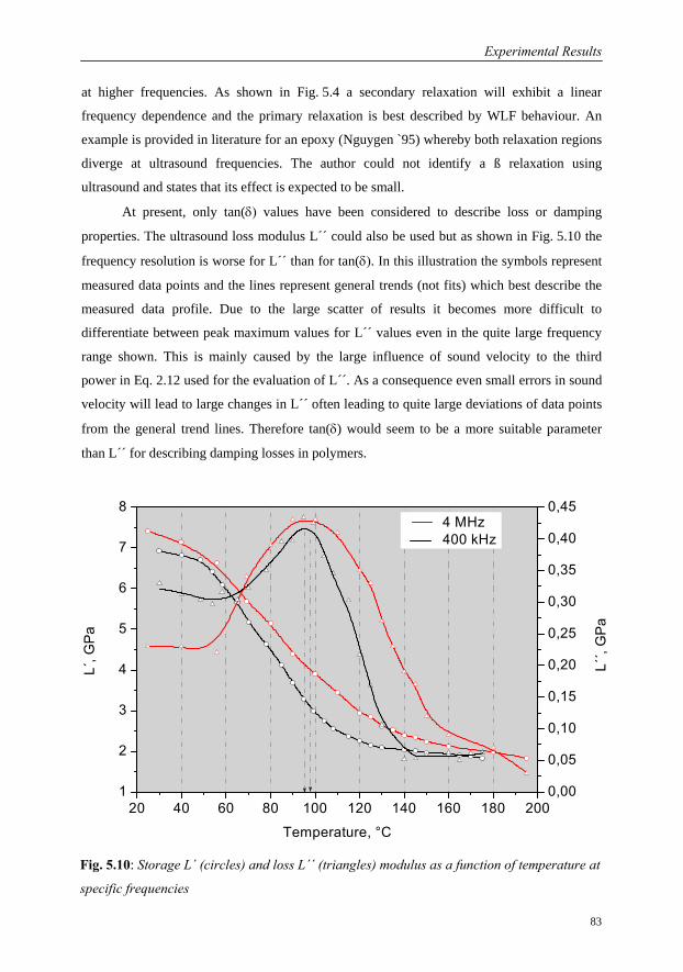
Experimental Results
83
at higher frequencies. As shown in Fig. 5.4 a secondary relaxation will exhibit a linear
frequency dependence and the primary relaxation is best described by WLF behaviour. An
example is provided in literature for an epoxy (Nguygen `95) whereby both relaxation regions
diverge at ultrasound frequencies. The author could not identify a ß relaxation using
ultrasound and states that its effect is expected to be small.
At present, only tan(δ) values have been considered to describe loss or damping
properties. The ultrasound loss modulus L´´ could also be used but as shown in Fig. 5.10 the
frequency resolution is worse for L´´ than for tan(δ). In this illustration the symbols represent
measured data points and the lines represent general trends (not fits) which best describe the
measured data profile. Due to the large scatter of results it becomes more difficult to
differentiate between peak maximum values for L´´ values even in the quite large frequency
range shown. This is mainly caused by the large influence of sound velocity to the third
power in Eq. 2.12 used for the evaluation of L´´. As a consequence even small errors in sound
velocity will lead to large changes in L´´ often leading to quite large deviations of data points
from the general trend lines. Therefore tan(δ) would seem to be a more suitable parameter
than L´´ for describing damping losses in polymers.
20 40 60 80 100 120 140 160 180 2001
2
3
4
5
6
7
8
0,00
0,05
0,10
0,15
0,20
0,25
0,30
0,35
0,40
0,45 4 MHz 400 kHz
L´´,
GP
a
L´, G
Pa
Temperature, °C
Fig. 5.10: Storage L´ (circles) and loss L´´ (triangles) modulus as a function of temperature at
specific frequencies
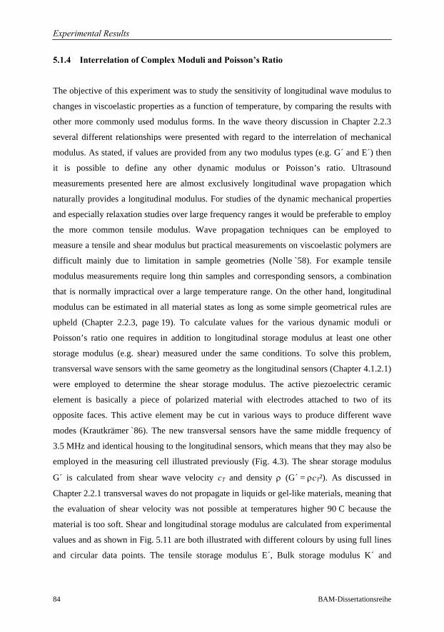
Experimental Results
84 BAM-Dissertationsreihe
5.1.4 Interrelation of Complex Moduli and Poisson’s Ratio
The objective of this experiment was to study the sensitivity of longitudinal wave modulus to
changes in viscoelastic properties as a function of temperature, by comparing the results with
other more commonly used modulus forms. In the wave theory discussion in Chapter 2.2.3
several different relationships were presented with regard to the interrelation of mechanical
modulus. As stated, if values are provided from any two modulus types (e.g. G´ and E´) then
it is possible to define any other dynamic modulus or Poisson’s ratio. Ultrasound
measurements presented here are almost exclusively longitudinal wave propagation which
naturally provides a longitudinal modulus. For studies of the dynamic mechanical properties
and especially relaxation studies over large frequency ranges it would be preferable to employ
the more common tensile modulus. Wave propagation techniques can be employed to
measure a tensile and shear modulus but practical measurements on viscoelastic polymers are
difficult mainly due to limitation in sample geometries (Nolle `58). For example tensile
modulus measurements require long thin samples and corresponding sensors, a combination
that is normally impractical over a large temperature range. On the other hand, longitudinal
modulus can be estimated in all material states as long as some simple geometrical rules are
upheld (Chapter 2.2.3, page 19). To calculate values for the various dynamic moduli or
Poisson’s ratio one requires in addition to longitudinal storage modulus at least one other
storage modulus (e.g. shear) measured under the same conditions. To solve this problem,
transversal wave sensors with the same geometry as the longitudinal sensors (Chapter 4.1.2.1)
were employed to determine the shear storage modulus. The active piezoelectric ceramic
element is basically a piece of polarized material with electrodes attached to two of its
opposite faces. This active element may be cut in various ways to produce different wave
modes (Krautkrämer `86). The new transversal sensors have the same middle frequency of
3.5 MHz and identical housing to the longitudinal sensors, which means that they may also be
employed in the measuring cell illustrated previously (Fig. 4.3). The shear storage modulus
G´ is calculated from shear wave velocity cT and density ρ (G´ = ρcT²). As discussed in
Chapter 2.2.1 transversal waves do not propagate in liquids or gel-like materials, meaning that
the evaluation of shear velocity was not possible at temperatures higher 90 C because the
material is too soft. Shear and longitudinal storage modulus are calculated from experimental
values and as shown in Fig. 5.11 are both illustrated with different colours by using full lines
and circular data points. The tensile storage modulus E´, Bulk storage modulus K´ and
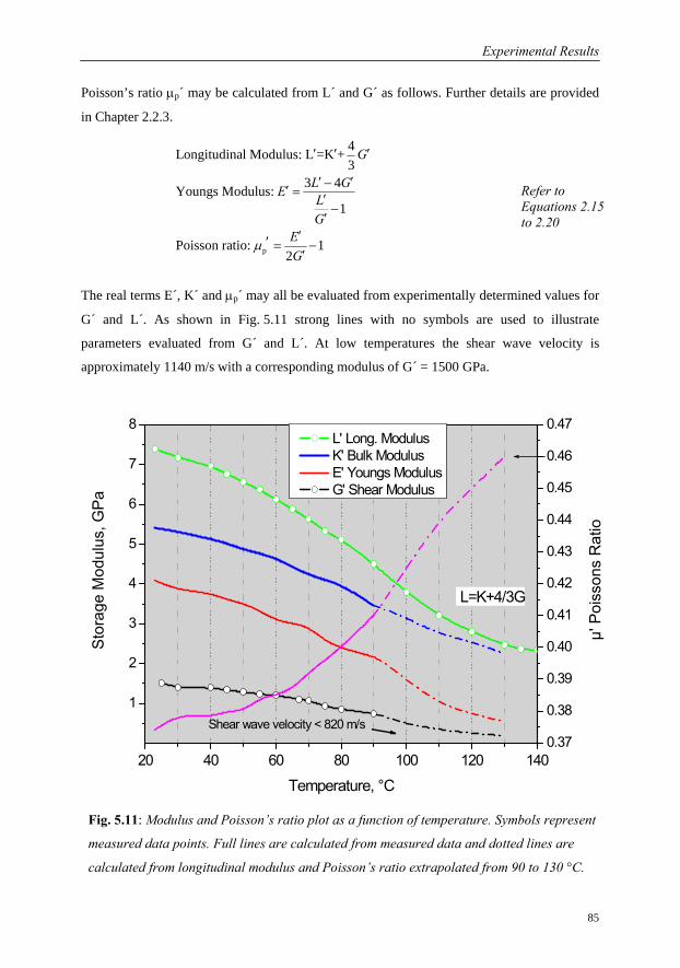
Experimental Results
85
Poisson’s ratio μp´ may be calculated from L´ and G´ as follows. Further details are provided
in Chapter 2.2.3.
The real terms E´, K´ and μp´ may all be evaluated from experimentally determined values for
G´ and L´. As shown in Fig. 5.11 strong lines with no symbols are used to illustrate
parameters evaluated from G´ and L´. At low temperatures the shear wave velocity is
approximately 1140 m/s with a corresponding modulus of G´ = 1500 GPa.
20 40 60 80 100 120 140
1
2
3
4
5
6
7
8
0.37
0.38
0.39
0.40
0.41
0.42
0.43
0.44
0.45
0.46
0.47
µ' P
oiss
ons
Rat
io
Sto
rage
Mod
ulus
, GP
a
Temperature, °C
L' Long. Modulus K' Bulk Modulus E' Youngs Modulus G' Shear Modulus
L=K+4/3G
Shear wave velocity < 820 m/s
Fig. 5.11: Modulus and Poisson’s ratio plot as a function of temperature. Symbols represent
measured data points. Full lines are calculated from measured data and dotted lines are
calculated from longitudinal modulus and Poisson’s ratio extrapolated from 90 to 130 °C.
p
4Longitudinal Modulus: L =K +3
3 4Youngs Modulus: 1
Poisson ratio: 12
′ ′ ′
′ ′−′ = ′−
′′′ = −′
G
L GE LG
EG
μ
Refer to Equations 2.15 to 2.20
Experimental Results
86 BAM-Dissertationsreihe
Shear waves propagate roughly 45 % slower than longitudinal waves and therefore the shear
storage modulus calculated using G´ = ρcT² is much lower than its longitudinal modulus
counterpart. Both measured moduli decrease with increasing temperature and in the vicinity
of the glass rubber transition at temperatures higher than 80 °C the signal to noise ratio
becomes so small that it is no longer possible to evaluate shear wave velocity with certainty.
The minimum velocity measured was approx. 820 m/s at 80 °C which would seem to
represent a critical lower level measurement limit for shear wave propagation (Döring `02).
From the determined values G´ and L´ it is possible to estimate the Poisson’s ratio using the
above equations. The calculated value of approx. 0.37 at 40 °C is typical for glassy polymers,
for example synthetic glass sapphire has a Poisson’s ratio of approx. 0.31. As already
explained at T > 90 °C it was impossible to evaluate shear data and therefore from
experimental data alone it would not be possible to calculate μp´. However from standard
material values it is known that for incompressible elastic solid the theoretical Poisson’s ratio
is about 0.5. For example natural rubber is quoted (Sperling `92) as having a Poisson’s ratio
of 0.49 and according to Alig (Alig ´02) an epoxy material in the rubber state at temperatures
above Tg has a value of 0.46. Considering this background, a value of 0.46 would seem to
provide a reasonable estimate for polymers in a rubberlike state and therefore the Poisson’s
ratio curve was extrapolated to a value of 0.46 at 130 °C. This temperature was chosen
because, as demonstrated in this chapter, this epoxy is definitely in the rubber state even for
experiments at MHz frequencies. Therefore the μp´ data measured up to 90 °C could be
extrapolated up to 130 °C. This extended curve is illustrated in the form of a dotted pink line.
As the longitudinal modulus is known throughout the whole temperature range (green line
with circular symbols), it is now possible using the data from the extrapolated Poisson’s ratio
to continue calculation of E´, K´ and also G´. At temperature above 90 °C these values are
also graphically illustrated using dashed lines. From the graphic illustration following
conclusions can be made:
• All modulus forms have similar profiles and each show a clear decrease with
temperature that is associated with the α relaxation.
• The magnitude values for the various storage moduli can be ordered in following
sequence, with L´ having the highest magnitude L´>K´>E´>G´. This behaviour is
expected as most materials resist a change in volume as determined by the bulk
modulus K´ more than they would resist a change in shape, as determined by the shear
Experimental Results
87
modulus G´. This result is easily visualised when one considers the load required
achieving compressional deformation in a polymer in comparison to forces required to
achieve a similar deformation using tensile or torsional loading techniques.
• A linear axis was chosen to best illustrate the results and one could quickly form an
incorrect opinion that the longitudinal modulus L´ is more sensitive than the shear
modulus G´ to changes in the viscoelastic properties due to what would seem to be a
larger change in modulus. This would also contradict the last statement (above). In
actual fact the opposite is true as G´ tends towards values in the hundred Pascal range.
This means changes in G´ could actually cover several orders of magnitude and will
therefore be more sensitive than a longitudinal or bulk compression modulus to
modulus variation independent of cause.
• At high temperatures higher than 90 °C the shear modulus G´ will tend towards very
low values because a viscous material cannot sustain shear wave propagation. Eq. 2.20
states L´ = K´ + 4/3G´ and shows that when G´ is low then the longitudinal storage
modulus L´ is nearly equal to the bulk storage modulus K´. This can be observed in
Fig. 5.11 at about 120 °C.
Experimental Results
88 BAM-Dissertationsreihe
5.2 Adaptation of Measuring Set-up for Cure Monitoring
In the previous section a two sample measuring set-up was employed to characterise a
cured epoxy. This was necessary because dynamic heating of both the epoxy sample and
sensors leads to a disproportionate change in impedance values between material boundaries
(see Eq. 4.4) making it difficult to accurately estimate the attenuation in the sample itself.
Ideally this technique should also work for curing epoxy systems, however the reaction is
exothermic and as a result the thicker the sample the more difficult it becomes to maintain or
guarantee constant sample temperatures (McHugh `03). On the other hand very thin samples
e.g. 1 mm may lead to errors in calculation of attenuation or sound velocity. A thickness error
of just 0.1 mm would consequently lead to deviations in sound velocity (Eq. 4.7) of about
10 %. Most authors in the past were mainly interested in obtaining quantitative values for
sound velocity whereas attenuation was only of secondary interest and therefore relative
values or simply, the change in attenuation over the curing reaction were normally deemed
sufficient for evaluation purposes. In such cases a measuring set-up using a single sample and
a reference sensor to sensor signal is employed (Döring `01) to obtain this information. In this
situation one of the two measured sample signals described under measurement principles
(Fig 4.7, Chapter 4.2) is replaced by a constant reference value at thickness null. To obtain
this reference signal the mould (Figs. 4.5 and 4.6) is fully closed so that the ultrasound
sensors are in direct contact and a thin layer of silicon oil of negligible thickness is used as
couple medium. The sound velocity and a relative attenuation are calculated as usual by
comparing these two signals (one constant and one variable) over the curing reaction.
In the cure monitoring experiments discussed in the following chapter a quantitative
value for attenuation is desired as it would facilitate a direct comparison with the DMA
results already presented. As all experiments take place at constant temperatures it is possible
to estimate if this new measurement setup will lead to significant errors in calculating
quantitative values for attenuation or if a correction factor is required. For this reason A-scan
signals were analysed at the start and end of cure. An evaluation example is provided below
in Fig. 5.12. The results show the A-scan signals obtained from the reference signal and a
3 mm epoxy sample at the beginning of cure at 60 °C whereby the epoxy has a low viscosity.
Impulse amplification was 40 dB for both reference and sample signal. The signals are
converted into their magnitude spectrum using the FFT analysis technique. Both signals are
similar in form and an attenuation loss in the 3 mm sample of 0.25 dB/mm was calculated at
3.5 MHz using Eq. 4.6. This attenuation value is quite low considering that the sound wave
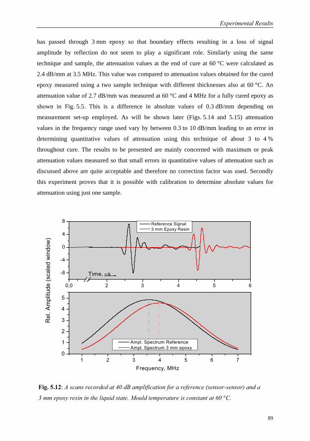
Experimental Results
89
has passed through 3 mm epoxy so that boundary effects resulting in a loss of signal
amplitude by reflection do not seem to play a significant role. Similarly using the same
technique and sample, the attenuation values at the end of cure at 60 °C were calculated as
2.4 dB/mm at 3.5 MHz. This value was compared to attenuation values obtained for the cured
epoxy measured using a two sample technique with different thicknesses also at 60 °C. An
attenuation value of 2.7 dB/mm was measured at 60 °C and 4 MHz for a fully cured epoxy as
shown in Fig. 5.5. This is a difference in absolute values of 0.3 dB/mm depending on
measurement set-up employed. As will be shown later (Figs. 5.14 and 5.15) attenuation
values in the frequency range used vary by between 0.3 to 10 dB/mm leading to an error in
determining quantitative values of attenuation using this technique of about 3 to 4 %
throughout cure. The results to be presented are mainly concerned with maximum or peak
attenuation values measured so that small errors in quantitative values of attenuation such as
discussed above are quite acceptable and therefore no correction factor was used. Secondly
this experiment proves that it is possible with calibration to determine absolute values for
attenuation using just one sample.
1 2 3 4 5 6 70
1
2
3
4
5
0,0 2 3 4 5 6
-8
-4
0
4
8
Rel
. Am
plitu
de (s
cale
d w
indo
w)
Frequency, MHz
Ampl. Spectrum Reference Ampl. Spectrum 3 mm epoxy
Time, μs
Reference Signal 3 mm Epoxy Resin
Fig. 5.12: A scans recorded at 40 dB amplification for a reference (sensor-sensor) and a
3 mm epoxy resin in the liquid state. Mould temperature is constant at 60 °C.
Experimental Results
90 BAM-Dissertationsreihe
5.3 Characterisation of Cure Behaviour
5.3.1 Introduction and Background
As discussed in the literature review in Chapter 2.1.3 acoustic parameters seem to be
sensitive to changes in the mechanical properties resulting from the growing network
structure. However, in the past the majority of research has relied largely on empirical
comparisons from a variety of analysis techniques that were based largely on differing
physical measurement principles e.g. dielectric analysis and NMR. This makes it very
difficult to form conclusions on how sensitive the acoustic technique is to chemorheological
changes occurring during cure and in particular transformations such as gelation and
vitrification. The objective of the following chapter is to investigate the sensitivity of
ultrasound sound velocity and tan(δ) to changes in the viscoelastic properties of a curing
epoxy polymer. To achieve this goal the results from ultrasound are compared to other more
common techniques used to characterise the curing reaction and changes in the viscoelastic
properties of a curing epoxy. Following a description of these changes, the main topics of this
section can be divided under following central themes:
Evaluation of isothermal cure experiments from each individual analysis
technique e.g. Ultrasound, DSC and Rheometric techniques.
General comparison of techniques and application of an Arrhenius based
relationship that provides an opportunity to quantitatively compare the
sensitivity of analysis techniques based on different measuring principles, but
which should all be sensitive to the curing reaction.
Discussion on the sensitivity of ultrasound to overall reaction and the
transformations: gelation and vitrification
Experimental Results
91
5.3.2 Interpretation of Isothermal Cure Profiles
5.3.2.1 Signal Analysis
Two signal analysis techniques are available that can be employed for the evaluation of sound
velocity and attenuation. The first is based on manual analysis of recorded A-scans using the
FFT analysis and was described in Chapter 4.2.1. The second technique uses the automatic
software “US-Plus system” developed at the BAM (Döring `02) and currently in use for
commercial applications in the field of cure monitoring. The main difference between the two
analysis techniques is that one is based on spectral analysis i.e. sound velocity and attenuation
data are evaluated as a function of frequency and the other is based on direct analysis of
ultrasound parameters from transmission times and signal amplitude over the whole
frequency bandwidth. To differentiate between the techniques, the second technique that is
mainly based on Peak Analysis will be referred to with the abbreviation PA. For the PA
technique, amplitude values are taken as the peak amplitude values for the first positive peak
observed in the sample and reference A-scans. Similarly transmission time is calculated by
subtracting the time taken to reach the first positive maximum in the sample A-scan from the
time to first positive maximum in the A-scan of the reference signal. This procedure is
standard evaluation practice in conventional acoustics. The main advantage of employing PA
is that measurement and evaluation takes place automatically in real-time by analysing peak
amplitudes and transmission times from the A-scans using specially developed software
(Döring `01). Once the sample amplitudes and transmission times have been recorded (using
FFT spectral analysis and PA techniques) then the same equations can be employed to
calculate attenuation and sound velocity (Eqs. 4.6 and 4.7). To illustrate the difference
between the two techniques, both were employed to analyse data obtained during epoxy cure
at 60 °C (see Figs. 5.13 and 5.14). As shown both evaluation techniques deliver similar sound
velocity and tan(δ) profiles over time and this general cure profile will be discussed before
commenting on specific differences between results. The sound velocity curves have a
sigmoidal form and can be split into three distinct regions (independent of evaluation method)
according to sound velocity magnitude.
Region 1: This region describes the low sound velocity values at the beginning of cure i.e. in
the range between 1450 to 1530 m/s depending on the measuring frequency. Filling and
closing the mould takes about 20 s and the epoxy assumes the environment temperature
immediately on filling due to the small amount of resin employed (less than 3 g). On filling a
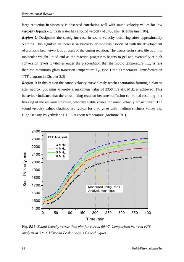
Experimental Results
92 BAM-Dissertationsreihe
large reduction in viscosity is observed correlating well with sound velocity values for low
viscosity liquids e.g. fresh water has a sound velocity of 1435 m/s (Krautkrämer `86).
Region 2: Designates the strong increase in sound velocity occurring after approximately
50 mins. This signifies an increase in viscosity or modulus associated with the development
of a crosslinked network as a result of the curing reaction. The epoxy resin starts life as a low
molecular weight liquid and as the reaction progresses begins to gel and eventually at high
conversion levels it vitrifies under the precondition that the mould temperature Tcure is less
than the maximum glass transition temperature Tg∞ (see Time Temperature Transformation
TTT diagram in Chapter 3.3).
Region 3: In this region the sound velocity curve slowly reaches saturation forming a plateau
after approx. 350 mins whereby a maximum value of 2350 m/s at 6 MHz is achieved. This
behaviour indicates that the crosslinking reaction becomes diffusion controlled resulting in a
freezing of the network structure, whereby stable values for sound velocity are achieved. The
sound velocity values obtained are typical for a polymer with medium stiffness values e.g.
High Density Polyethylene HDPE at room temperature (McIntire `91).
0 50 100 150 200 250 300 350 4001400
1500
1600
1700
1800
1900
2000
2100
2200
2300
2400FFT Analysis
3 MHz 4 MHz 5 MHz 6 MHz
Measured using Peak Analysis technique
Sou
nd V
eloc
ity, m
/s
Time, min
Fig. 5.13: Sound velocity versus time plot for cure at 60 °C. Comparison between FFT
analysis at 3 to 6 MHz and Peak Analysis PA techniques.
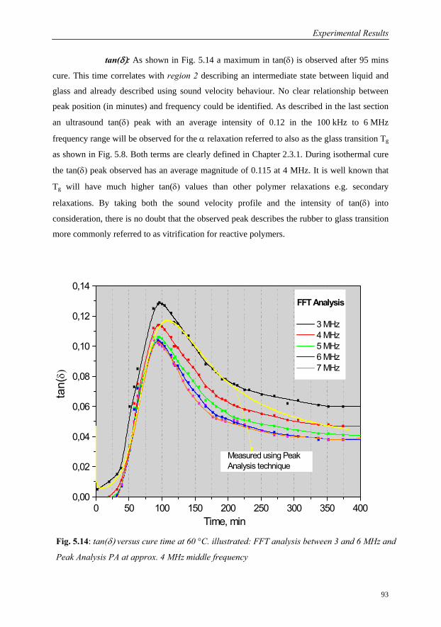
Experimental Results
93
tan(δ): As shown in Fig. 5.14 a maximum in tan(δ) is observed after 95 mins
cure. This time correlates with region 2 describing an intermediate state between liquid and
glass and already described using sound velocity behaviour. No clear relationship between
peak position (in minutes) and frequency could be identified. As described in the last section
an ultrasound tan(δ) peak with an average intensity of 0.12 in the 100 kHz to 6 MHz
frequency range will be observed for the α relaxation referred to also as the glass transition Tg
as shown in Fig. 5.8. Both terms are clearly defined in Chapter 2.3.1. During isothermal cure
the tan(δ) peak observed has an average magnitude of 0.115 at 4 MHz. It is well known that
Tg will have much higher tan(δ) values than other polymer relaxations e.g. secondary
relaxations. By taking both the sound velocity profile and the intensity of tan(δ) into
consideration, there is no doubt that the observed peak describes the rubber to glass transition
more commonly referred to as vitrification for reactive polymers.
0 50 100 150 200 250 300 350 4000,00
0,02
0,04
0,06
0,08
0,10
0,12
0,14FFT Analysis
3 MHz 4 MHz 5 MHz 6 MHz 7 MHz
tan(
δ)
Time, min
Measured using Peak Analysis technique
Fig. 5.14: tan(δ) versus cure time at 60 °C. illustrated: FFT analysis between 3 and 6 MHz and
Peak Analysis PA at approx. 4 MHz middle frequency
Experimental Results
94 BAM-Dissertationsreihe
Comments on Analysis Techniques: In Figs. 5.13 and 5.14 the colour yellow signifies
measurements using the PA technique. One major disadvantage of this technique is that
frequency specific information may be lost. However as the sensors operate in a limited
frequency bandwidth of approx. 5 MHz as shown in Fig. 5.12, large errors resulting from
assuming a middle frequency are not to be expected. To calculate tan(δ) = αλ/π using this
technique values for both attenuation α and wavelength λ are required. Wavelength is
calculated from sound velocity c and the frequency f is taken as constant at 4 MHz, associated
with the sensor middle frequency (see Fig. 5.12). The middle frequency is an average value
and will typically drift during cure by about ± 0.5 MHz, depending on extent of cure. This
explains slight deviations of the yellow tan (δ) curve from the frequency dependent
measurements using FFT analysis at 4 MHz. Frequency dependence of sound velocity or
dispersion is well known in polymer materials (see Chapter 2.2.4). If during cure a constant or
middle frequency is assumed as is the case using the PA technique then dispersion effects will
be neglected leading to a deviation of yellow sound velocity line from values measured at a
specific frequencies e.g. red line at 4 MHz both illustrated in Fig. 5.13. To summarise; results
will vary slightly depending on analysis technique employed but the same crucial information
will remain, for example cure times required until sound velocity increases or reaches
saturation and also a maximum in tan(δ) is observed after similar cure times. The main
advantage of using PA over FFT analysis is that ultrasound parameters can be evaluated
automatically in real time, saving considerable evaluation time, especially where large
amounts of data need to be evaluated.
5.3.2.2 Characterisation of Cure Behaviour at Constant Temperatures
Ultrasound measurements were performed at temperatures between 40 and 100 °C using the
PA evaluation technique. To help compare the results with other characterisation methods,
characteristic cure times common to the isothermal cure profiles were identified as shown in
Fig. 5.15 at 60 °C. tonset describes the cure time at which a strong increase in sound velocity is
observed. tOffset is the turnover time employed to define the cure time required until the sound
velocity curve begins to saturate, after which only a very gradual increase in sound velocity is
identified. Both turning points are defined by the crossing of two tangents drawn in the area
of interest as shown in Fig. 5.15. tOffset times are difficult to determine with high accuracy
because their positions will vary depending on how the tangents are placed and should only
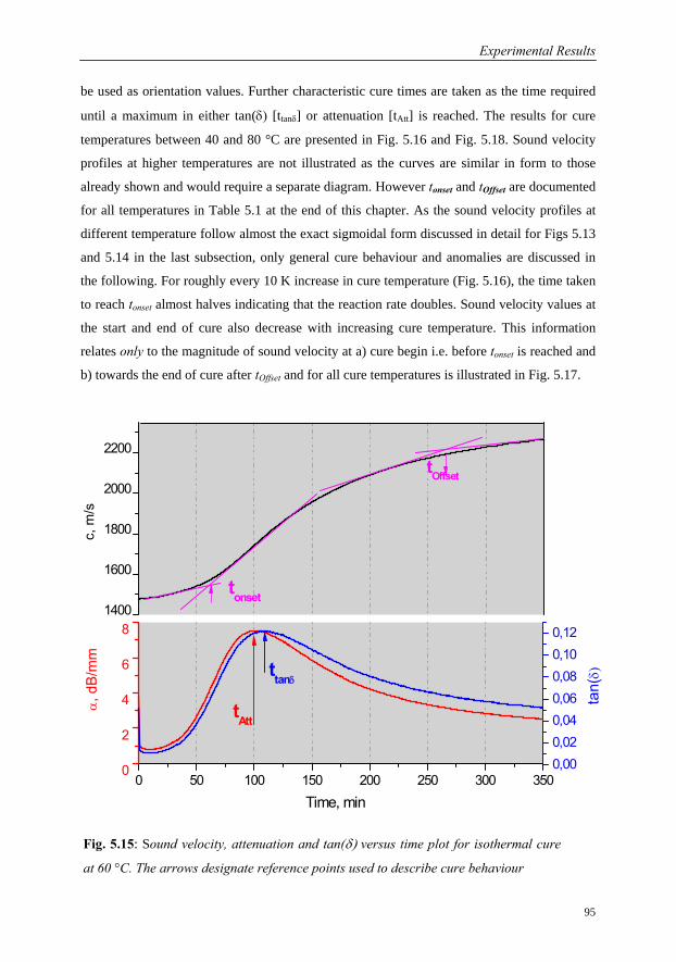
Experimental Results
95
be used as orientation values. Further characteristic cure times are taken as the time required
until a maximum in either tan(δ) [ttanδ] or attenuation [tAtt] is reached. The results for cure
temperatures between 40 and 80 °C are presented in Fig. 5.16 and Fig. 5.18. Sound velocity
profiles at higher temperatures are not illustrated as the curves are similar in form to those
already shown and would require a separate diagram. However tonset and tOffset are documented
for all temperatures in Table 5.1 at the end of this chapter. As the sound velocity profiles at
different temperature follow almost the exact sigmoidal form discussed in detail for Figs 5.13
and 5.14 in the last subsection, only general cure behaviour and anomalies are discussed in
the following. For roughly every 10 K increase in cure temperature (Fig. 5.16), the time taken
to reach tonset almost halves indicating that the reaction rate doubles. Sound velocity values at
the start and end of cure also decrease with increasing cure temperature. This information
relates only to the magnitude of sound velocity at a) cure begin i.e. before tonset is reached and
b) towards the end of cure after tOffset and for all cure temperatures is illustrated in Fig. 5.17.
1400
1600
1800
2000
2200
0 50 100 150 200 250 300 3500
2
4
6
8
0,000,020,040,060,080,100,12
tOffset
tan(
δ)
α, d
B/m
m
Time, min
c, m
/s
tonset
ttanδ
tAtt
Fig. 5.15: Sound velocity, attenuation and tan(δ) versus time plot for isothermal cure
at 60 °C. The arrows designate reference points used to describe cure behaviour
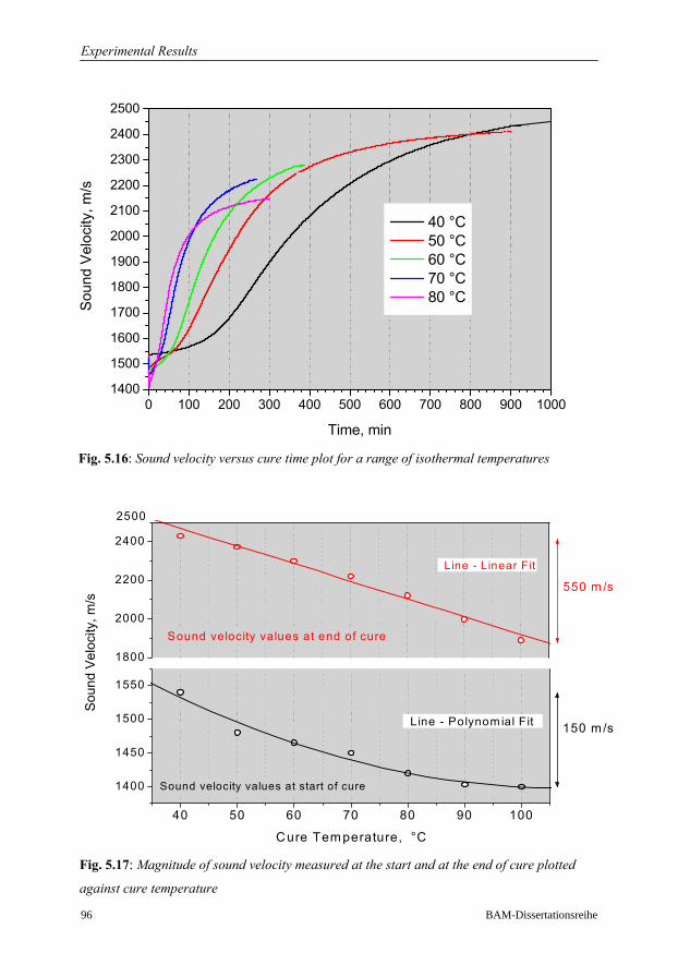
Experimental Results
96 BAM-Dissertationsreihe
0 100 200 300 400 500 600 700 800 900 10001400
1500
1600
1700
1800
1900
2000
2100
2200
2300
2400
2500
40 °C 50 °C 60 °C 70 °C 80 °CS
ound
Vel
ocity
, m/s
Time, min
Fig. 5.16: Sound velocity versus cure time plot for a range of isothermal temperatures
1800
2000
2200
2400
40 50 60 70 80 90 100
1400
1450
1500
1550
Sou
nd V
eloc
ity, m
/s
150 m /s
550 m /s
Line - Linear Fit
Sound velocity values at end of cure
2500
Line - Polynom ial Fit
Cure Tem perature, °C
Sound velocity values at start of cure
Fig. 5.17: Magnitude of sound velocity measured at the start and at the end of cure plotted
against cure temperature
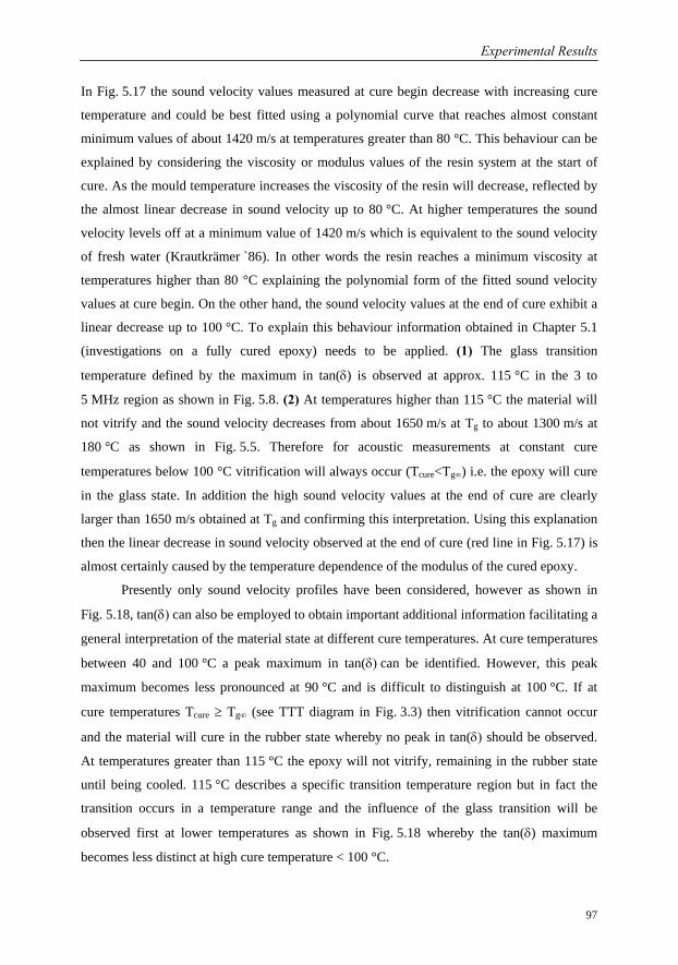
Experimental Results
97
In Fig. 5.17 the sound velocity values measured at cure begin decrease with increasing cure
temperature and could be best fitted using a polynomial curve that reaches almost constant
minimum values of about 1420 m/s at temperatures greater than 80 °C. This behaviour can be
explained by considering the viscosity or modulus values of the resin system at the start of
cure. As the mould temperature increases the viscosity of the resin will decrease, reflected by
the almost linear decrease in sound velocity up to 80 °C. At higher temperatures the sound
velocity levels off at a minimum value of 1420 m/s which is equivalent to the sound velocity
of fresh water (Krautkrämer `86). In other words the resin reaches a minimum viscosity at
temperatures higher than 80 °C explaining the polynomial form of the fitted sound velocity
values at cure begin. On the other hand, the sound velocity values at the end of cure exhibit a
linear decrease up to 100 °C. To explain this behaviour information obtained in Chapter 5.1
(investigations on a fully cured epoxy) needs to be applied. (1) The glass transition
temperature defined by the maximum in tan(δ) is observed at approx. 115 °C in the 3 to
5 MHz region as shown in Fig. 5.8. (2) At temperatures higher than 115 °C the material will
not vitrify and the sound velocity decreases from about 1650 m/s at Tg to about 1300 m/s at
180 °C as shown in Fig. 5.5. Therefore for acoustic measurements at constant cure
temperatures below 100 °C vitrification will always occur (Tcure<Tg∞) i.e. the epoxy will cure
in the glass state. In addition the high sound velocity values at the end of cure are clearly
larger than 1650 m/s obtained at Tg and confirming this interpretation. Using this explanation
then the linear decrease in sound velocity observed at the end of cure (red line in Fig. 5.17) is
almost certainly caused by the temperature dependence of the modulus of the cured epoxy.
Presently only sound velocity profiles have been considered, however as shown in
Fig. 5.18, tan(δ) can also be employed to obtain important additional information facilitating a
general interpretation of the material state at different cure temperatures. At cure temperatures
between 40 and 100 °C a peak maximum in tan(δ) can be identified. However, this peak
maximum becomes less pronounced at 90 °C and is difficult to distinguish at 100 °C. If at
cure temperatures Tcure ≥ Tg∞ (see TTT diagram in Fig. 3.3) then vitrification cannot occur
and the material will cure in the rubber state whereby no peak in tan(δ) should be observed.
At temperatures greater than 115 °C the epoxy will not vitrify, remaining in the rubber state
until being cooled. 115 °C describes a specific transition temperature region but in fact the
transition occurs in a temperature range and the influence of the glass transition will be
observed first at lower temperatures as shown in Fig. 5.18 whereby the tan(δ) maximum
becomes less distinct at high cure temperature < 100 °C.
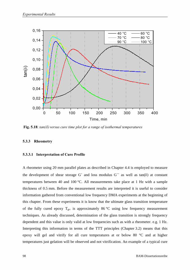
Experimental Results
98 BAM-Dissertationsreihe
5.3.3 Rheometry
5.3.3.1 Interpretation of Cure Profile
A rheometer using 20 mm parallel plates as described in Chapter 4.4 is employed to measure
the development of shear storage G´ and loss modulus G´´ as well as tan(δ) at constant
temperatures between 40 and 100 °C. All measurements take place at 1 Hz with a sample
thickness of 0.5 mm. Before the measurement results are interpreted it is useful to consider
information gathered from conventional low frequency DMA experiments at the beginning of
this chapter. From these experiments it is know that the ultimate glass transition temperature
of the fully cured epoxy Tg∞ is approximately 86 °C using low frequency measurement
techniques. As already discussed, determination of the glass transition is strongly frequency
dependent and this value is only valid at low frequencies such as with a rheometer. e.g. 1 Hz.
Interpreting this information in terms of the TTT principles (Chapter 3.2) means that this
epoxy will gel and vitrify for all cure temperatures at or below 80 °C and at higher
temperatures just gelation will be observed and not vitrification. An example of a typical cure
0 50 100 150 200 250 300 350 4000,00
0,02
0,04
0,06
0,08
0,10
0,12
0,14
0,16ta
n(δ)
Time, min
40 °C 60 °C 70 °C 80 °C 90 °C 100 °C
Fig. 5.18: tan(δ) versus cure time plot for a range of isothermal temperatures
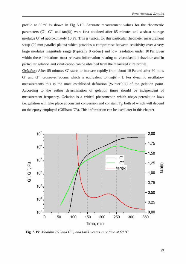
Experimental Results
99
profile at 60 °C is shown in Fig. 5.19. Accurate measurement values for the rheometric
parameters (G´, G´´ and tan(δ)) were first obtained after 85 minutes and a shear storage
modulus G´ of approximately 10 Pa. This is typical for this particular rheometer measurement
setup (20 mm parallel plates) which provides a compromise between sensitivity over a very
large modulus magnitude range (typically 8 orders) and low resolution under 10 Pa. Even
within these limitations most relevant information relating to viscoelastic behaviour and in
particular gelation and vitrification can be obtained from the measured cure profile.
Gelation: After 85 minutes G´ starts to increase rapidly from about 10 Pa and after 90 mins
G´ and G´´ crossover occurs which is equivalent to tan(δ) = 1. For dynamic oscillatory
measurements this is the most established definition (Winter `97) of the gelation point.
According to the author determination of gelation times should be independent of
measurement frequency. Gelation is a critical phenomenon which obeys percolation laws
i.e. gelation will take place at constant conversion and constant Tg; both of which will depend
on the epoxy employed (Gillham `73). This information can be used later in this chapter.
0 50 100 150 200 250 300 350101
102
103
104
105
106
107
0,000,00
0,25
0,500,50
0,75
1,001,00
1,25
1,501,50
1,75
2,002,00
G' G''
tan(
δ)
G´,
G´´,
Pa
Time, min
tan(δ)
Fig. 5.19: Modulus (G´ and G´´) and tanδ versus cure time at 60 °C
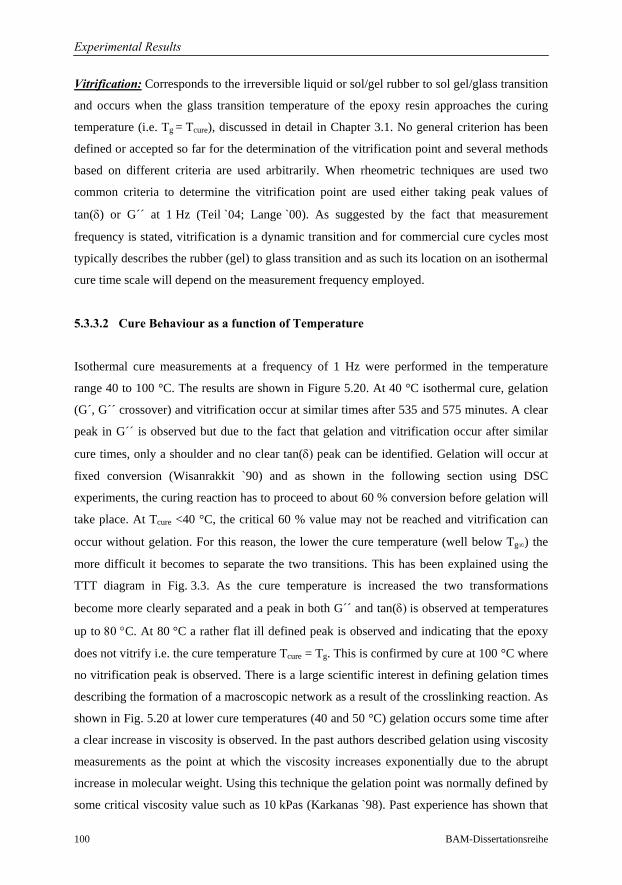
Experimental Results
100 BAM-Dissertationsreihe
Vitrification: Corresponds to the irreversible liquid or sol/gel rubber to sol gel/glass transition
and occurs when the glass transition temperature of the epoxy resin approaches the curing
temperature (i.e. Tg = Tcure), discussed in detail in Chapter 3.1. No general criterion has been
defined or accepted so far for the determination of the vitrification point and several methods
based on different criteria are used arbitrarily. When rheometric techniques are used two
common criteria to determine the vitrification point are used either taking peak values of
tan(δ) or G´´ at 1 Hz (Teil `04; Lange `00). As suggested by the fact that measurement
frequency is stated, vitrification is a dynamic transition and for commercial cure cycles most
typically describes the rubber (gel) to glass transition and as such its location on an isothermal
cure time scale will depend on the measurement frequency employed.
5.3.3.2 Cure Behaviour as a function of Temperature
Isothermal cure measurements at a frequency of 1 Hz were performed in the temperature
range 40 to 100 °C. The results are shown in Figure 5.20. At 40 °C isothermal cure, gelation
(G´, G´´ crossover) and vitrification occur at similar times after 535 and 575 minutes. A clear
peak in G´´ is observed but due to the fact that gelation and vitrification occur after similar
cure times, only a shoulder and no clear tan(δ) peak can be identified. Gelation will occur at
fixed conversion (Wisanrakkit `90) and as shown in the following section using DSC
experiments, the curing reaction has to proceed to about 60 % conversion before gelation will
take place. At Tcure <40 °C, the critical 60 % value may not be reached and vitrification can
occur without gelation. For this reason, the lower the cure temperature (well below Tg∞) the
more difficult it becomes to separate the two transitions. This has been explained using the
TTT diagram in Fig. 3.3. As the cure temperature is increased the two transformations
become more clearly separated and a peak in both G´´ and tan(δ) is observed at temperatures
up to 80 °C. At 80 °C a rather flat ill defined peak is observed and indicating that the epoxy
does not vitrify i.e. the cure temperature Tcure = Tg. This is confirmed by cure at 100 °C where
no vitrification peak is observed. There is a large scientific interest in defining gelation times
describing the formation of a macroscopic network as a result of the crosslinking reaction. As
shown in Fig. 5.20 at lower cure temperatures (40 and 50 °C) gelation occurs some time after
a clear increase in viscosity is observed. In the past authors described gelation using viscosity
measurements as the point at which the viscosity increases exponentially due to the abrupt
increase in molecular weight. Using this technique the gelation point was normally defined by
some critical viscosity value such as 10 kPas (Karkanas `98). Past experience has shown that
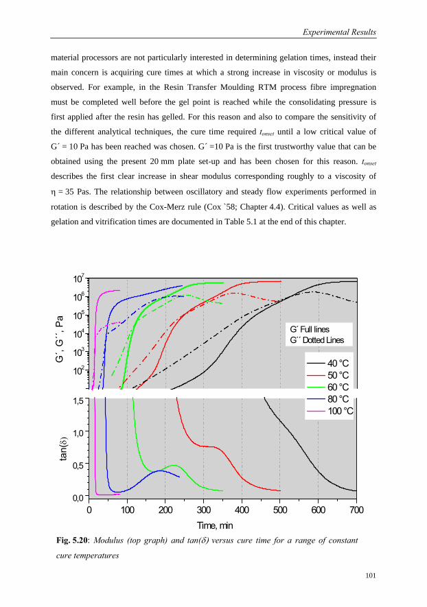
Experimental Results
101
Fig. 5.20: Modulus (top graph) and tan(δ) versus cure time for a range of constant
cure temperatures
101
102
103
104
105
106
107
0 100 200 300 400 500 600 7000,0
0,5
1,0
1,5
G Full linesG Dotted Lines
40 °C 50 °C 60 °C 80 °C 100 °C
Time, min
tan(
δ)G
´, G
´´, P
amaterial processors are not particularly interested in determining gelation times, instead their
main concern is acquiring cure times at which a strong increase in viscosity or modulus is
observed. For example, in the Resin Transfer Moulding RTM process fibre impregnation
must be completed well before the gel point is reached while the consolidating pressure is
first applied after the resin has gelled. For this reason and also to compare the sensitivity of
the different analytical techniques, the cure time required tonset until a low critical value of
G´ = 10 Pa has been reached was chosen. G´ =10 Pa is the first trustworthy value that can be
obtained using the present 20 mm plate set-up and has been chosen for this reason. tonset
describes the first clear increase in shear modulus corresponding roughly to a viscosity of
η = 35 Pas. The relationship between oscillatory and steady flow experiments performed in
rotation is described by the Cox-Merz rule (Cox `58; Chapter 4.4). Critical values as well as
gelation and vitrification times are documented in Table 5.1 at the end of this chapter.
Experimental Results
102 BAM-Dissertationsreihe
5.3.4 Dynamic Scanning Calorimetry DSC
5.3.4.1 Degree of Cure and Cure Profile
DSC provides information on the extent of the curing reaction in terms of evolution of the
fractional degree of cure (most often referred to as fractional conversion α). By heating the
epoxy sample to 300 °C in a dynamic heating run at 10 K/min, it is possible to obtain the
total exothermic heat of reaction released during the curing reaction from the area enclosed
under a thermogram (see Eq. 4.27, p64). It can be confirmed that the reaction has proceeded
to 100 % by a consecutive heating run or rescan. By determining the exothermic heat of
reaction for either isothermal or dynamic cure runs and placing it in relationship to total cure
it is possible to determine fractional conversion for a particular cure cycle (see Figure 5.21).
More detailed example is provided in Fig. 4.14 and with help of Eqs. 4.23 to 4.24.
0.00
0.05
0.10
0.15
0.20
0 50 100 150 200 250 3000
20
40
60
80
100
Hea
t Flo
w, m
W/m
g
Exotherm
Frac
. Con
vers
ion,
%
Time, min
Fig. 5.21: Exothermic heat flow for cure at 80 °C (top half). The area under the curve is
determined by integration and presented as percentage of the total heat of reaction in terms
of conversion
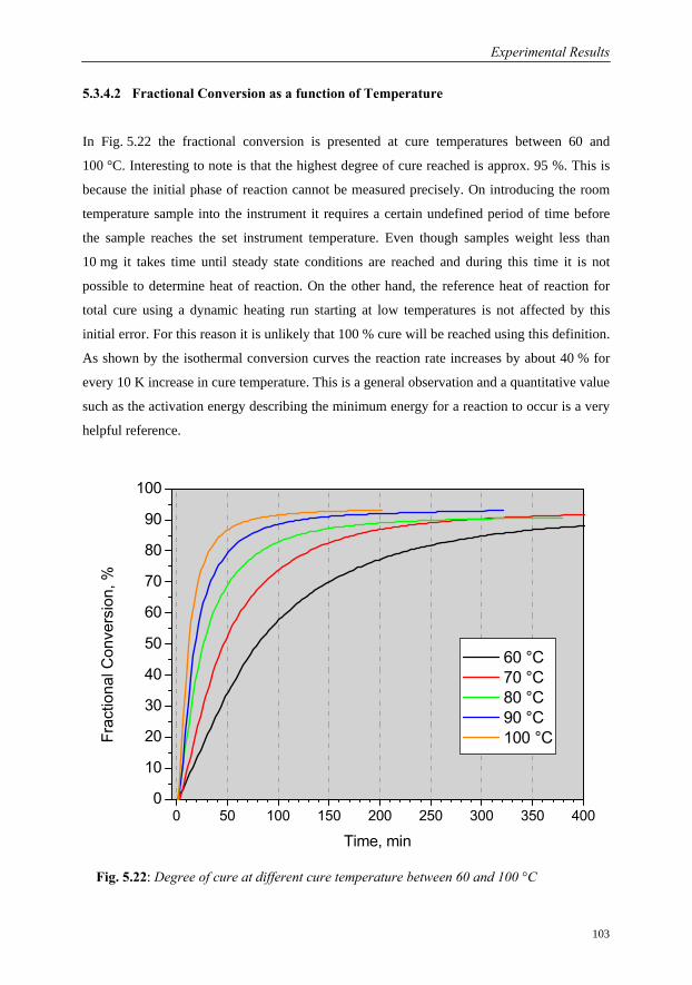
Experimental Results
103
5.3.4.2 Fractional Conversion as a function of Temperature
In Fig. 5.22 the fractional conversion is presented at cure temperatures between 60 and
100 °C. Interesting to note is that the highest degree of cure reached is approx. 95 %. This is
because the initial phase of reaction cannot be measured precisely. On introducing the room
temperature sample into the instrument it requires a certain undefined period of time before
the sample reaches the set instrument temperature. Even though samples weight less than
10 mg it takes time until steady state conditions are reached and during this time it is not
possible to determine heat of reaction. On the other hand, the reference heat of reaction for
total cure using a dynamic heating run starting at low temperatures is not affected by this
initial error. For this reason it is unlikely that 100 % cure will be reached using this definition.
As shown by the isothermal conversion curves the reaction rate increases by about 40 % for
every 10 K increase in cure temperature. This is a general observation and a quantitative value
such as the activation energy describing the minimum energy for a reaction to occur is a very
helpful reference.
0 50 100 150 200 250 300 350 4000
10
20
30
40
50
60
70
80
90
100
Frac
tiona
l Con
vers
ion,
%
Time, min
60 °C 70 °C 80 °C 90 °C 100 °C
Fig. 5.22: Degree of cure at different cure temperature between 60 and 100 °C
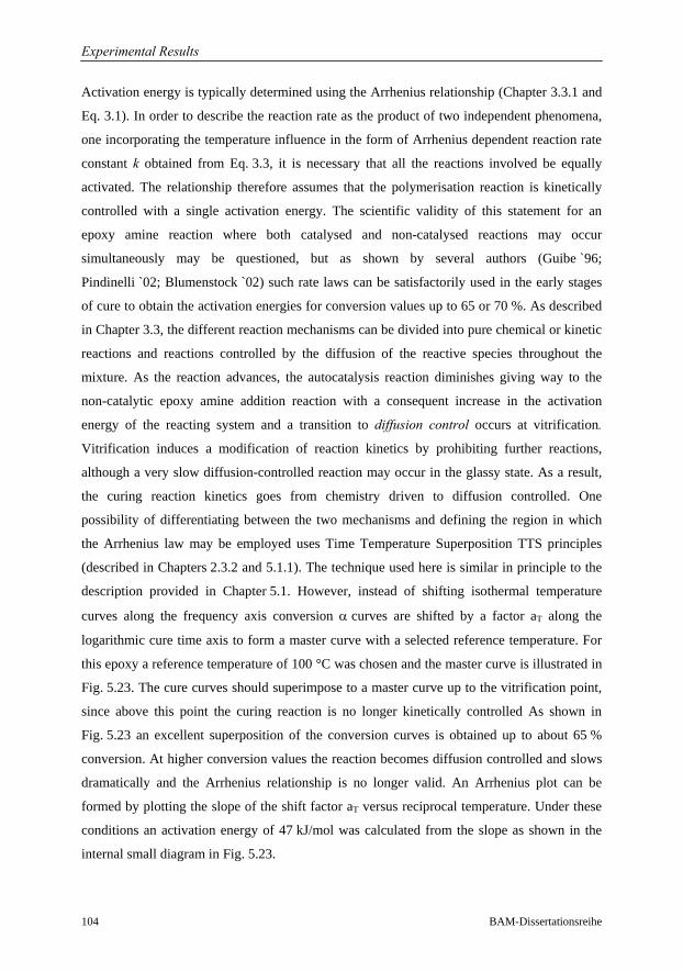
Experimental Results
104 BAM-Dissertationsreihe
Activation energy is typically determined using the Arrhenius relationship (Chapter 3.3.1 and
Eq. 3.1). In order to describe the reaction rate as the product of two independent phenomena,
one incorporating the temperature influence in the form of Arrhenius dependent reaction rate
constant k obtained from Eq. 3.3, it is necessary that all the reactions involved be equally
activated. The relationship therefore assumes that the polymerisation reaction is kinetically
controlled with a single activation energy. The scientific validity of this statement for an
epoxy amine reaction where both catalysed and non-catalysed reactions may occur
simultaneously may be questioned, but as shown by several authors (Guibe `96;
Pindinelli `02; Blumenstock `02) such rate laws can be satisfactorily used in the early stages
of cure to obtain the activation energies for conversion values up to 65 or 70 %. As described
in Chapter 3.3, the different reaction mechanisms can be divided into pure chemical or kinetic
reactions and reactions controlled by the diffusion of the reactive species throughout the
mixture. As the reaction advances, the autocatalysis reaction diminishes giving way to the
non-catalytic epoxy amine addition reaction with a consequent increase in the activation
energy of the reacting system and a transition to diffusion control occurs at vitrification.
Vitrification induces a modification of reaction kinetics by prohibiting further reactions,
although a very slow diffusion-controlled reaction may occur in the glassy state. As a result,
the curing reaction kinetics goes from chemistry driven to diffusion controlled. One
possibility of differentiating between the two mechanisms and defining the region in which
the Arrhenius law may be employed uses Time Temperature Superposition TTS principles
(described in Chapters 2.3.2 and 5.1.1). The technique used here is similar in principle to the
description provided in Chapter 5.1. However, instead of shifting isothermal temperature
curves along the frequency axis conversion α curves are shifted by a factor aT along the
logarithmic cure time axis to form a master curve with a selected reference temperature. For
this epoxy a reference temperature of 100 °C was chosen and the master curve is illustrated in
Fig. 5.23. The cure curves should superimpose to a master curve up to the vitrification point,
since above this point the curing reaction is no longer kinetically controlled As shown in
Fig. 5.23 an excellent superposition of the conversion curves is obtained up to about 65 %
conversion. At higher conversion values the reaction becomes diffusion controlled and slows
dramatically and the Arrhenius relationship is no longer valid. An Arrhenius plot can be
formed by plotting the slope of the shift factor aT versus reciprocal temperature. Under these
conditions an activation energy of 47 kJ/mol was calculated from the slope as shown in the
internal small diagram in Fig. 5.23.
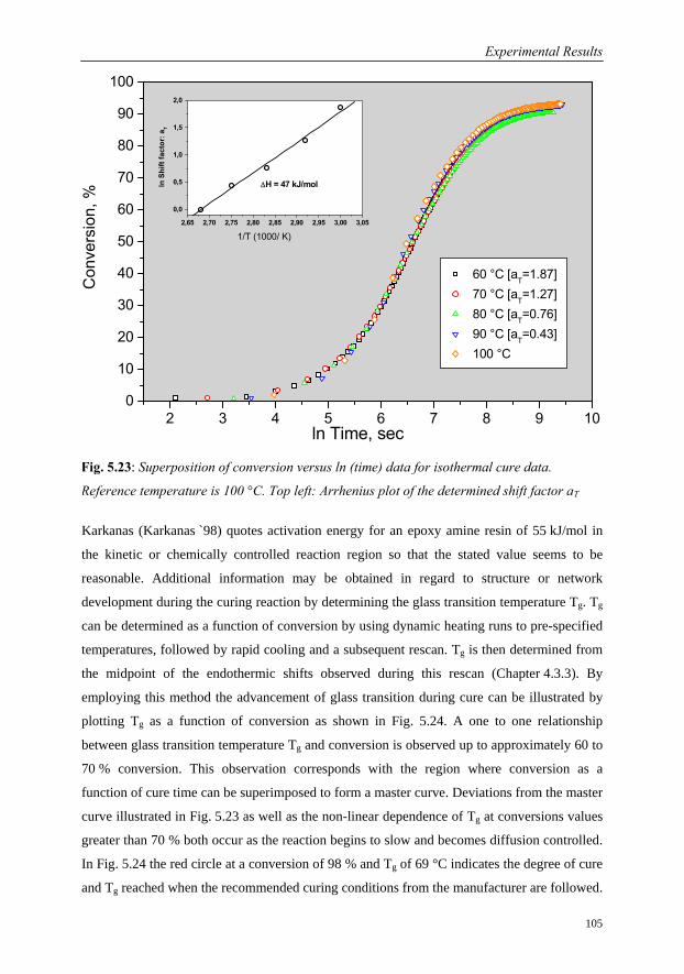
Experimental Results
105
Karkanas (Karkanas `98) quotes activation energy for an epoxy amine resin of 55 kJ/mol in
the kinetic or chemically controlled reaction region so that the stated value seems to be
reasonable. Additional information may be obtained in regard to structure or network
development during the curing reaction by determining the glass transition temperature Tg. Tg
can be determined as a function of conversion by using dynamic heating runs to pre-specified
temperatures, followed by rapid cooling and a subsequent rescan. Tg is then determined from
the midpoint of the endothermic shifts observed during this rescan (Chapter 4.3.3). By
employing this method the advancement of glass transition during cure can be illustrated by
plotting Tg as a function of conversion as shown in Fig. 5.24. A one to one relationship
between glass transition temperature Tg and conversion is observed up to approximately 60 to
70 % conversion. This observation corresponds with the region where conversion as a
function of cure time can be superimposed to form a master curve. Deviations from the master
curve illustrated in Fig. 5.23 as well as the non-linear dependence of Tg at conversions values
greater than 70 % both occur as the reaction begins to slow and becomes diffusion controlled.
In Fig. 5.24 the red circle at a conversion of 98 % and Tg of 69 °C indicates the degree of cure
and Tg reached when the recommended curing conditions from the manufacturer are followed.
Fig. 5.23: Superposition of conversion versus ln (time) data for isothermal cure data.
Reference temperature is 100 °C. Top left: Arrhenius plot of the determined shift factor aT
2 3 4 5 6 7 8 9 100
10
20
30
40
50
60
70
80
90
100
2,65 2,70 2,75 2,80 2,85 2,90 2,95 3,00 3,05
0,0
0,5
1,0
1,5
2,0
ln Time, sec
Con
vers
ion,
%
60 °C [aT=1.87] 70 °C [aT=1.27] 80 °C [aT=0.76] 90 °C [aT=0.43] 100 °C
ΔH = 47 kJ/mol
1/T (1000/ K)
ln S
hift
fact
or: a
T
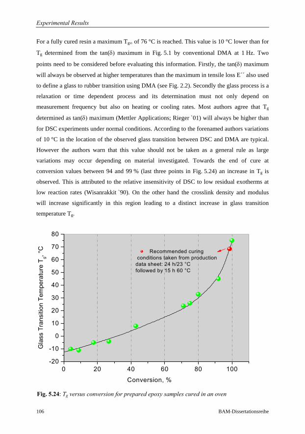
Experimental Results
106 BAM-Dissertationsreihe
For a fully cured resin a maximum Tg∞ of 76 °C is reached. This value is 10 °C lower than for
Tg determined from the tan(δ) maximum in Fig. 5.1 by conventional DMA at 1 Hz. Two
points need to be considered before evaluating this information. Firstly, the tan(δ) maximum
will always be observed at higher temperatures than the maximum in tensile loss E´´ also used
to define a glass to rubber transition using DMA (see Fig. 2.2). Secondly the glass process is a
relaxation or time dependent process and its determination must not only depend on
measurement frequency but also on heating or cooling rates. Most authors agree that Tg
determined as tan(δ) maximum (Mettler Applications; Rieger `01) will always be higher than
for DSC experiments under normal conditions. According to the forenamed authors variations
of 10 °C in the location of the observed glass transition between DSC and DMA are typical.
However the authors warn that this value should not be taken as a general rule as large
variations may occur depending on material investigated. Towards the end of cure at
conversion values between 94 and 99 % (last three points in Fig. 5.24) an increase in Tg is
observed. This is attributed to the relative insensitivity of DSC to low residual exotherms at
low reaction rates (Wisanrakkit `90). On the other hand the crosslink density and modulus
will increase significantly in this region leading to a distinct increase in glass transition
temperature Tg.
0 20 40 60 80 100-20
-10
0
10
20
30
40
50
60
70
80
Recommended curing conditions taken from productiondata sheet: 24 h/23 °C followed by 15 h 60 °C
Gla
ss T
rans
ition
Tem
pera
ture
Tg, °
C
Conversion, %
Fig. 5.24: Tg versus conversion for prepared epoxy samples cured in an oven
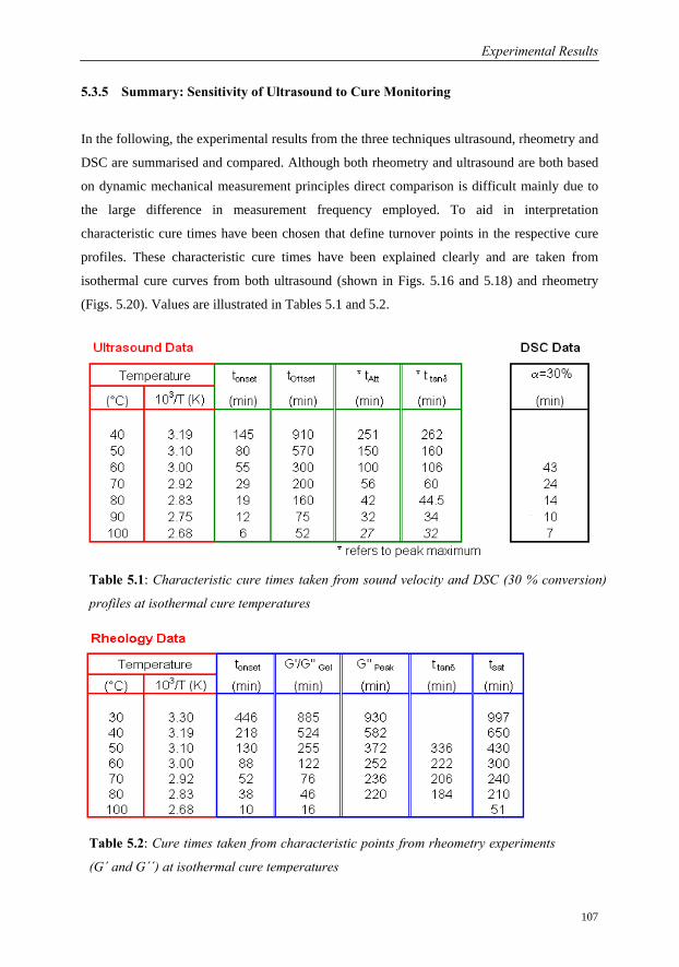
Experimental Results
107
5.3.5 Summary: Sensitivity of Ultrasound to Cure Monitoring
In the following, the experimental results from the three techniques ultrasound, rheometry and
DSC are summarised and compared. Although both rheometry and ultrasound are both based
on dynamic mechanical measurement principles direct comparison is difficult mainly due to
the large difference in measurement frequency employed. To aid in interpretation
characteristic cure times have been chosen that define turnover points in the respective cure
profiles. These characteristic cure times have been explained clearly and are taken from
isothermal cure curves from both ultrasound (shown in Figs. 5.16 and 5.18) and rheometry
(Figs. 5.20). Values are illustrated in Tables 5.1 and 5.2.
Table 5.2: Cure times taken from characteristic points from rheometry experiments
(G´ and G´´) at isothermal cure temperatures
Table 5.1: Characteristic cure times taken from sound velocity and DSC (30 % conversion)
profiles at isothermal cure temperatures
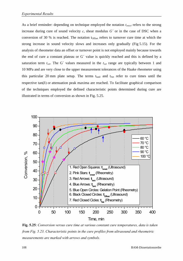
Experimental Results
108 BAM-Dissertationsreihe
As a brief reminder: depending on technique employed the notation tonset refers to the strong
increase during cure of sound velocity c, shear modulus G´ or in the case of DSC when a
conversion of 30 % is reached. The notation tOffset refers to turnover cure time at which the
strong increase in sound velocity slows and increases only gradually (Fig 5.15). For the
analysis of rheometer data an offset or turnover point is not employed mainly because towards
the end of cure a constant plateau or G´ value is quickly reached and this is defined by a
saturation term tsat. The G´ values measured in the tsat range are typically between 1 and
10 MPa and are very close to the upper measurement tolerances of the Haake rheometer using
this particular 20 mm plate setup. The terms ttanδ and tAtt refer to cure times until the
respective tan(δ) or attenuation peak maxima are reached. To facilitate graphical comparison
of the techniques employed the defined characteristic points determined during cure are
illustrated in terms of conversion as shown in Fig. 5.25.
Fig. 5.25: Conversion versus cure time at various constant cure temperatures, data is taken
from Fig. 5.23. Characteristic points in the cure profiles from ultrasound and rheometric
measurements are marked with arrows and symbols.
0 50 100 150 200 250 300 350 4000
10
20
30
40
50
60
70
80
90
100
***
Con
vers
ion,
%
Time, min
60 °C 70 °C 80 °C 90 °C 100 °C
*1. Red Open Squares: tonset (Ultrasound)2. Pink Stars: tonset (Rheometry)3. Red Arrows: ttanδ
(Ultrasound)4. Blue Arrows: ttanδ
(Rheometry)5. Blue Open Circles: Gelation Point (Rheometry)6. Black Closed Circles: tOffset (Ultrasound)7. Red Closed Cicles: tSat (Rheometry)
Experimental Results
109
From this illustration following observations were made:
• Cure Begin: A large increase in sound velocity tonset (red squares) is observed before
any results could be evaluated from rheometric experiments. tonset for rheometric
experiments was chosen as G´ = 10 Pa representing the lower critical measurement
limit for the 20 mm plates setup employed for this experiment. Accurate values for G´
below 10 Pa were not obtained as shown in Fig. 5.20. For ultrasound experiments tonset
represents the large increase in sound velocity defined in Fig. 5.15 and occurs for all
cure temperatures at conversion values below 40 %. Even before tonset is reached a
gradual increase in sound velocity is observed. This is corroborated by Fig. 5.17
showing that even small changes in viscosity at the start of cure may be distinguished
by differences in sound velocity magnitude.
• Gelation point: This point is defined by the crossover of G´ and G´´ in rheometry.
Shortly after the increase in sound velocity, the shear modulus tonset (rheometric
measurements) increases dramatically and gelation occurs at approx. 62 to 65 %
conversion. These values indicate the accuracy of the results, as according to
publications discussed in Chapters 3.2 gelation should occur at constant conversion
and Tg independent of cure temperature. Also, conversion values of about 60 % are
typical for stoichiometric mixtures of epoxy systems (Mc Hugh `01; Nunez `05).
• End of Cure: The end of cure is defined as the region in which the reaction becomes
diffusion controlled and was determined experimentally as shown in Fig.5.23. This
occurs at 65 to 70 % conversion correlating well with gelation point. The saturation or
plateau region of the conversion curves marks the cessation of the reaction. As shown
both G´ and sound velocity can be measured close to the end of reaction at all cure
temperatures. However for rheometric experiments it is no longer possible to obtain
trustworthy results almost immediately after vitrification i.e. after tan(δ) maximum is
reached as shown in Fig. 5.19. This is the upper measurement limit of this rheometer
set-up. At similar cure times sound velocity also reaches tOffset (black closed circles).
After this turnover time is reached sound velocity only increases gradually as shown
in Fig. 5.16. It was demonstrated in Fig. 5.24 that even a small increase in conversion
of about 5 % towards the end of cure can cause a significant increase in Tg. Small
changes in conversion occurring at the end of cure are hardly negligible using DSC
but will lead to an increase in crosslink density and modulus. The results indicate that
sound velocity is a highly sensitive parameter capable of detecting changes in modulus
occurring after vitrification.
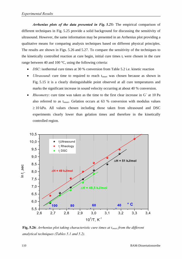
Experimental Results
110 BAM-Dissertationsreihe
Arrhenius plots of the data presented in Fig. 5.25: The empirical comparison of
different techniques in Fig. 5.25 provide a solid background for discussing the sensitivity of
ultrasound. However, the same information may be presented in an Arrhenius plot providing a
qualitative means for comparing analysis techniques based on different physical principles.
The results are shown in Figs. 5.26 and 5.27. To compare the sensitivity of the techniques to
the kinetically controlled reaction at cure begin, initial cure times ti were chosen in the cure
range between 40 and 100 °C, using the following criteria:
• DSC: isothermal cure times at 30 % conversion from Table 5.2 i.e. kinetic reaction
• Ultrasound: cure time to required to reach tonset was chosen because as shown in
Fig. 5.15 it is a clearly distinguishable point observed at all cure temperatures and
marks the significant increase in sound velocity occurring at about 40 % conversion.
• Rheometry: cure time was taken as the time to the first clear increase in G´ at 10 Pa
also referred to as tonset. Gelation occurs at 63 % conversion with modulus values
≥ 10 kPa. All values chosen including those taken from ultrasound and DSC
experiments clearly lower than gelation times and therefore in the kinetically
controlled region.
2,6 2,7 2,8 2,9 3,0 3,1 3,2 3,3 3,45,5
6,0
6,5
7,0
7,5
8,0
8,5
9,0
9,5
10,0
10,5
tiUltrasound ti Rheology ti DSC
ΔH = 49 kJ/mol
ΔH = 51 kJ/mol
ΔH = 48,5 kJ/mol
ln t i ,s
ec
103/T, K-1
100 80 60 40 ° C
Fig, 5.26: Arrhenius plot taking characteristic cure times at tonset from the different
analytical techniques (Tables 5.1 and 5.2).
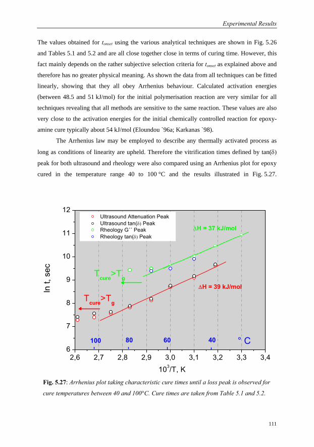
Experimental Results
111
The values obtained for tonset using the various analytical techniques are shown in Fig. 5.26
and Tables 5.1 and 5.2 and are all close together close in terms of curing time. However, this
fact mainly depends on the rather subjective selection criteria for tonset as explained above and
therefore has no greater physical meaning. As shown the data from all techniques can be fitted
linearly, showing that they all obey Arrhenius behaviour. Calculated activation energies
(between 48.5 and 51 kJ/mol) for the initial polymerisation reaction are very similar for all
techniques revealing that all methods are sensitive to the same reaction. These values are also
very close to the activation energies for the initial chemically controlled reaction for epoxy-
amine cure typically about 54 kJ/mol (Eloundou `96a; Karkanas `98).
The Arrhenius law may be employed to describe any thermally activated process as
long as conditions of linearity are upheld. Therefore the vitrification times defined by tan(δ)
peak for both ultrasound and rheology were also compared using an Arrhenius plot for epoxy
cured in the temperature range 40 to 100 °C and the results illustrated in Fig. 5.27.
2,6 2,7 2,8 2,9 3,0 3,1 3,2 3,3 3,46
7
8
9
10
11
12
Tcure>Tg
Ultrasound Attenuation Peak Ultrasound tan(δ) Peak Rheology G´´ Peak Rheology tan(δ) Peak
ΔH = 37 kJ/mol
ΔH = 39 kJ/mol
100
103/T, K
80 60
ln t,
sec
40 ° C
Tcure>Tg
Fig. 5.27: Arrhenius plot taking characteristic cure times until a loss peak is observed for
cure temperatures between 40 and 100°C. Cure times are taken from Table 5.1 and 5.2.
Experimental Results
112 BAM-Dissertationsreihe
As additional information the cure times for loss peak in attenuation from ultrasound and
shear loss modulus G´´ from rheometry were also plotted in the same diagram
The activation energies calculated of 39 and 37 kJ/mol are very similar for both DMA
techniques presented and correlate well with values obtained by Guibe (Guibe `96) using
DSC experiments whereby the author describes vitrification time as cure time required until
Tcure=Tg (see Chapter 3.2). However, the determined values should not be confused with
activation energy for the diffusion controlled reaction and the estimated energies simply
provide a good means to compare two different analysis techniques. The actual physical
meaning of the absolute values and their application is unclear at present. The time scale of
the experiment illustrates that the loss peak associated with vitrification will be observed first
with the ultrasound technique. As shown in Chapter 5.1 determination of the temperature at
which the glass transition is observed will depend strongly on the measurement frequency of
the technique employed. Using ultrasound as DMA at 4 MHz and conventional DMA
experiments at 1 Hz the respective Tg∞ values determined were 115 °C and 86 °C as shown in
Fig. 5.8. Therefore deviations from linearity occur at temperatures at which a glass rubber
transition is no longer distinguished using the respective analysis technique i.e. at Tcure ≥ Tg∞
when the selected cure temperature approaches the maximum achievable Tg∞ of the epoxy
system.
Comments: Sensitivity of the Acoustic Parameters to Gelation
One recurring question with regard to ultrasound investigations on a curing resin has
not been clearly answered. Is the measured sound velocity or attenuation sensitive to
gelation taking place during epoxy cure? The simple answer is no! The reason that gelation
point is conventionally taken as the crossover point G´and G´´ or tan(δ) = 1 and should be
independent of measurement frequency at 1 Hz (Winter `87) although the same author admits
that there are some exceptions to this rule (Winter `97). Ultrasound measurements have been
performed to a high accuracy and throughout cure tan(δ) has remained smaller than 0.13 so
that according to classical convention ultrasound parameters will not be influenced by
gelation. Explanation for the insensitivity of ultrasound to gelation as defined by the
percolation theory (not to be confused with increase in viscosity) may result from the nature
of longitudinal waves. It is known that for longitudinal wave measurement that the following
equation describes the relationship between longitudinal storage L´, bulk storage K´ and shear
storage G´ module:
Experimental Results
113
L´=K´+4/3G´ see Eq. 2.18
Shear waves do not propagate in liquids and are first observed after gelation (Parthun `95).
Therefore before gelation L´=K´ meaning that only a compression wave can propagate in the
polymer. Losses in polymers due to internal friction or damping will be significantly lower
for dynamic compression than for tensile or shear loading experiments (Murayama `78). This
is corroborated by the low intensity values for tan(δ) values obtained for ultrasound
measurements in comparison to values obtained by conventional DMA (see Figs. 5.1 and
5.20). For this reason the differences in storage modulus will not be as striking for a measured
longitudinal modulus as for shear modulus that will change by several orders of magnitude
during cure. Taking these points into consideration a definition of gelation as the crossover
between L´ and L´´ or tan(δ) =1 is unlikely to be fulfilled for dynamic compression
experiments.
Another possible explanation for this apparent insensitivity to gelation may be
demonstrated using Fig. 5.25. In this figure the glass transition is observed for all cure
temperatures either before or in close vicinity to gelation. Determination of gelation should be
independent of frequency as explained above whereas the rubber-glass transition temperature
taken as the tan(δ) maximum is not and is observed much earlier at high acoustic
measurement frequencies than for rheometer experiments (see Fig. 5.25) For this reason, in
the temperature range employed even if this acoustic techniques were sensitive to gelation, it
would most likely be overshadowed by vitrification.
114 BAM-Dissertationsreihe
Chapter 6
6 Conclusions
It is well know that acoustic wave propagation can be employed to determine the dynamic
modulus of polymers. However, several questions remain open in regard to the sensitivity of
the determined longitudinal modulus L´ particularly in comparison to more conventional
modulus values e.g. shear G´ or tensile E´ storage modulus measured using conventional
DMA performed at low frequencies. The academic potential of this acoustic technique is
presently only limited by complications in an exact interpretation of results. If wave
propagation techniques are employed for DMA of material properties several additional
factors may influence quantitative determination of L´, L´´ or tan(δ). Amongst others, they
include the high frequency of measurement, acoustic coupling of sensors, amplitude losses at
boundaries and temperature stability of sensors. These points were taken into consideration as
follows:
A two sample measuring setup was constructed so that boundary effects
(reflections) leading to a large decrease in amplitude could be neglected
Fast Fourier Transformation analysis software was developed so that
frequency specific sound velocity and attenuation could be determined
In order to obtain data over a wider range of frequency high temperature
sensors in the 2 to 6 MHz and 250 to 650 kHz range were employed.
To study the influence of the glass rubber transition on measurement results, a
commercial epoxy was chosen with a glass rubber transition Tg of 86 °C i.e.
well within the limits of the ultrasound and DMA techniques measuring range.
Integration of these factors into experimental setup and evaluation strategy means that enough
accurate acoustic data are available over a large frequency and temperature range to make
credible conclusions on the application of ultrasound as a DMA technique.
Conclusions
115
The experimental results are divided into two main sections: investigations on a fully
cured and on a reactive epoxy resin. In the first section all investigations took place on a fully
cured epoxy with a glass rubber transition at approximately 86 °C as defined by a
tan(δ) maximum at 1 Hz. The results from ultrasound longitudinal and in just one example for
shear wave propagation were compared to conventional DMA. The main topics covered are
briefly introduced and demonstrate the application potential of ultrasound as a high frequency
DMA technique:
Acoustic Parameters: L´, L´´ and tan(δ) were evaluated as a function of frequency
from the ultrasound parameters sound velocity and attenuation. The term
αc/ω<< 1 was calculated and has a maximum value of 0.08 even in the α relaxation
region that is associated with high damping. Therefore reduced equations will almost
always be valid for unfilled polymers and can be employed to calculate L´, L´´ and
tan(δ). Material damping properties are best described using tan(δ). This loss factor
has the added advantage that it can easily calculated from acoustic parameters and is
common to all DMA techniques. The elastic modulus is typically expressed using L´
but because change of density is negligible then sound velocity c ∝√ L´ and may also
be used to express changes in viscoelastic properties.
Influence of Frequency: By analysing the results from conventional DMA in the
frequency range 0.1 to 50 Hz and using the Williams Landel Ferry WLF equation it
was possible to predict the influence of measurement frequencies on the determination
of the α relaxation. The model correlated well with experimental results evaluated at
specific frequencies in the ranges 400 to 800 kHz and 2 to 5 MHz. Clearly shown was
that the α relaxation observed at 86 °C at 1 Hz will be observed at 118 °C at 4 MHz or
approx. a shift of 5 K per decade increase in measurement frequency.
Interrelation of Modulus: By measuring both shear and longitudinal wave propagation
for the epoxy system as a function of temperature in the range 20 to 200 °C their
respective storage moduli G´ and L´ could be determined. From these parameters the
bulk K´ and tensile E´ storage moduli as well as the real part of Poisson’s ratio µ´ can
be calculated. This provides the background necessary to understand the interrelation
of the different dynamic moduli as well as Poisson’s ratio. More importantly it
demonstrated the sensitivity of the longitudinal modulus to changes in the viscoelastic
properties.
Conclusions
116 BAM-Dissertationsreihe
The second section of this thesis is concerned with determining the sensitivity of
sound velocity and attenuation to changes in the viscoelastic properties of a curing resin i.e.
application of ultrasound as a cure monitoring technique. Sound velocity and attenuation or
tan(δ) are compared to the results from other laboratory analysis techniques, all measured
over a range of constant cure temperatures between 40 and 100 °C. Differential Scanning
Calorimeter DSC is employed to obtain information relating to the extent of the curing
reaction and network formation. A rheometer is also employed as DMA technique to monitor
variations in G´ and tan(δ) during the curing reaction. To discuss the sensitivity of the
ultrasound technique the cure process is divided under the following four headings:
Start of Cure: Sound velocity increases gradually at the start of cure with a large
increase occurring at approx. 40% conversion and referred to as tonset. Using a rheometer
measured values for the storage G´ modulus could first be determined after approx. 50 %
conversion. As discussed, for conversion values below 60 % the reaction remains kinetically
controlled which means that the activation energy for the reaction can be calculated using the
Arrhenius equation. The respective activation energies calculated for Ultrasound, Rheometer
and DSC techniques were 51, 49 and 48.5 KJ/mol providing a clear indication that all
methods are sensitive to the same initial polymerisation reaction.
Gelation Point: No evidence indicates that sound velocity is sensitive to gelation
according to conventional definitions such as tan(δ)=1. Possible reasons are that measured
tan(δ) values obtained using compressional or longitudinal loading forces had a maximum
value of 0.14 or well under the above gelation criteria. Another explanation for the apparent
insensitivity of ultrasound to gelation was demonstrated using Fig. 5.25. In this figure the
glass transition is observed for all cure temperatures either before or in close vicinity to
gelation. Determination of gelation should be independent of frequency as explained above
whereas the rubber-glass transition temperature taken as the tan(δ) maximum is not and is
observed much earlier in the MHz frequency range than at low frequencies used for rheometer
experiments. For this reason, even if acoustic techniques are sensitive to gelation for this
epoxy it is most likely that gelation would be overshadowed by vitrification. Although, the
results show that a specific gelation point could not be identified, the continued increase in
sound velocity in this region indicates a high sensitivity to changes in viscosity or modulus as
the curing reaction proceeds.
Vitrification: it was demonstrated that the ultrasound tan(δ) peak observed at different
cure temperatures is caused by vitrification. Maximum values of tan(δ)=0.14 are obtained at
Conclusions
117
vitrification and provide excellent correlation with values obtained for the glass rubber
transition for ultrasound investigations on the fully cured epoxy discussed in Chapter 5.1. At
vitrification the reaction becomes diffusion controlled and a gradual change of material state
from gel/rubber to a glassy state occurs. This rubber-glass transition is a dynamic transition
and during cure will be observed at shorter cure times the higher the measurement frequency
employed. For this reason the tan(δ) peak will be observed at shorter cure times for ultrasound
than for rheometric experiments.
End of Cure: Vitrification induces a modification of the reaction kinetics by
prohibiting further reactions, although a very slow diffusion controlled reaction may occur in
the glassy state. DSC is relatively insensitive to this latter reaction as conversion reaches
saturation shortly after vitrification. It is only with subsequent rescans that an increase in Tg
can be detected proving the epoxy has reacted further. The results confirm that even small
changes in conversion that are difficult to measure using DSC lead to an increase in crosslink
density and modulus. At present the only DMA technique capable of providing quantitative
storage modulus values over the whole curing reaction is the ultrasound wave propagation
technique presented in this work. For isothermal cure, even the newer rheological instruments
require at least one change of plates (large plates for liquid to rubberlike state and small plates
for the rubber to glass-like state) or at least two separate experiments pro cure temperature
before a change in modulus can be accurately measured throughout cure.
Application for Cure Monitoring: The main advantage of ultrasound over most
laboratory based analysis techniques is that it is based on wave propagation principles so that
only relatively small sensors are required to provide information on the viscoelastic state of
polymers. The sensors employed here are temperature resistance to 190 °C and can easily be
incorporated into most production processes. By using a dry coupling technique with copper
foil as couple medium modern sensors can even be mounted behind the mould wall so that
marking of the moulding does not take place. These factors combined with the high
sensitivity of this technique for DMA of polymer materials demonstrates its potential for a
range of applications.
118 BAM-Dissertationsreihe
Suggestions for Further Work
The ultrasound cure monitoring technique “US Plus” is currently in use for several
commercial applications in the field of injection moulding of thermosetting powder
compounds e.g. Phenol or Urea Formaldehyde. Other applications include flow front and cure
monitoring of epoxy based compounds reinforced with carbon or glass fibre e.g Resin
Transfer Moulding RTM. The work presented here is intended to aid interpretation of results
and to fill existing gaps in knowledge regarding the accuracy of this technique in-particular to
understand relationships between storage and loss modulus and tan(δ) and the measured
ultrasound parameters. The experiments were performed on neat or virgin resin materials to
avoid further complicating interpretation and to minimise sources of potential error. Futher
work will continue particularly in directions relating to possible future commercial
applications.
Continued development of ultrasound system and evaluation techniques for new
applications such as the characterisation of Carbon Fibre Reinforced Plastics
CFRP. This will mean taking the information published here a step further and
applying it to fibre reinforced composites whereby additional problems such as
scattering on fibre interfaces, voids, or filler combinations may have to be
considered.
Future applications especially in the materials science field will most likely
involve the combination of sound velocity analysis with kinetic models for the
prediction of cure behaviour. Such predictive models are commonly used in
combination with DSC but as mentioned in the literature review are not common
for DMA techniques.
The ultrasound technique has shown great potential for cure monitoring especially
when employed in combination with other analysis techniques such as rheometry.
One possibility would be to develop an ultrasound technique for laboratory
application for example employing a larger frequency bandwidth than used here
and with an additional oven enabling dynamic heating and cooling runs.
119
References
Adabbo, E., Williams, R. J .J., “The Evolution of Thermosetting Polymers in a Conversion-
Temperature Phase Diagram”, Journal of Applied Polymer Science, 27, 1327, (1982)
Aklonis, J. J., MacKnight, W. J., Shen, M., “Introduction to Polymer Viscoelasticity”, Wiley-
Interscience New York, London, (1972)
Alig, I., Fedtke, M., Häusler, K. G., Tänzer, W., Wartewig, S., “Modified Epoxies as Studied
by Ultrasonic Methods”, Progr. Colloid Poly. Sci., 78, 54, (1988)
Alig, I., Häusler, K., Nancke, K., Tänzer, W., Wartewig, S., “Ultraschalluntersuchungen zur
Bildung von diolmodifizierten Epoxidharznetzwerken”, Acta Polymerica, 40, 508, (1989)
Alig, I., “Ultrasonic Relaxation and Complex Heat Capacity”, Thermochimica Acta, 35, 304,
(1997)
Alig, I., Lellinger, D., Tadjbakhsch, S., “Sonic Methods for Characterising Polymeric
Materials’’, Polymeric Materials Science and Engineering, 79, 31, (1998)
Alig, I., Nancke, K., Johari, G. P., “Relaxation in Thermosets XXVI. Ultrasonic Studies of the
Temperature Dependence of Curing Kinetics of Diglycidyl Ether of Bisphenol A with
Catalyst”, Journal of Polymer Science: Part B, 32, 1465, (1994)
Alig, I., Tadjbakash, S., Zosel, A., “Comparison of Ultrasonic Shear Wave and Dynamic-
Mechanical Measurement in Acrylic-Type Copolymers”, Journal of Polymer Science: Part
B., 36, 1793, (1998)
American Society for Testing and Materials ASTM E698: “Standard Test Method for
Arrhenius Kinetic Constants for Thermally Unstable Materials”, (1984)
Asay, J. R., Lamerson, D.L., Guenther, A.H., “Pressure and Temperature Dependence of
Acoustic Velocities in Polymethylmethacrylate”, Journal of Applied Physics, 40, 1768,
(1968)
References
120 BAM-Dissertationsreihe
Babayevsky, P. G., Gillham, J. K., “Epoxy Thermosetting Systems: Dynamic Mechanical
Analysis of the Reactions of Aromatic Diamines with the Diglycidyl Ether of Bisphenol A”,
Journal of Applied Polymer Science, 17, 2067, (1973)
Blumenstock, T., “Analyse der Eigenspannungen während der Aushärtung von Epoxidharz-
massen”, PhD Thesis, University of Stuttgart, (2002)
Borchardt, H.-J., Daniels, F. ,“The Application of Differential Thermal Analysis to the Study
of Reaction Kinetics”, Journal American Chemical Society, 79, 41, (1957)
Brockman, N.L., Eisenberg, A., “The Bulk viscoelastic Properties of Poly(styrene –co-sodium
styrene-p-carboxylate)”, Journal of Polymer Science: Polymer Physics Edition, 23, 1145,
(1985)
Brown, E. C., Olley, P., Coates, P. D., “In Line Temperature Measurement during Real Time
Ultrasound Monitoring of Single Screw Extrusion”, Plastics, Rubber and Composites, 29, 3,
(2000)
Brydson, J. A., Plastics Materials, 6th Edition, Butterworth-Heinemann, Oxford, 1995
Challis, R. E., “Viscoelasticity of thin Adhesive Layers as a function of Cure and Service
Temperature Measured by a Novel Technique”, Journal of Applied Polymer Science, 44, 65,
(1992)
Challis, R. E., Cocker, R. P., Chadwick, D. L., Dare, D. J., Martin, C., Mahendrasingam, A.,
Fuller, W., “Ultrasonic Measurements related to Evolution of Structure in Curing Epoxy
Resins”, Plastics, Rubber and Composites, 29, 110, (2000)
Challis, R. E., Unwin, M. E., Chadwick, D. L., Freemantle, R. J., Partridge, I. K., Dare, D. J.,
Karkanas, P. I., “Following Network Formation in an Epoxy/Amine by Ultrasound, Dielectric
and Nuclear Magnetic Resonance Measurements: A Comparative Study, Journal of Applied
Polymer Science, 88, 1665, (2003)

References
121
Choy, I. C, Plazek, D. J, “The Physical Properties of Bisphenol—Based Epoxy Resins during
and after Curing”, Journal of Polymer Science: Part B: Polymer Physics, 24, 1303, (1986)
Chow, A.W., Bellin, J. L., “Simultaneous Acoustic Wave Propagation and Dynamic
Mechanical Analysis of Curing of Thermoset Resins”, Polymer Engineering and Science, 32,
182, (1992)
Cowie, J. M. G., “Polymers Chemistry & Physics of Modern Materials”, 2nd Edt., Blackie
Glasgow and London, (1991)
Cox, W.P., Merz, E.H., “Correlation of Dynamic and Steady Flow Viscosities”, Journal of
Polymer Science, 28, 619, (1958)
Cunningham, J. R., Ivey, D.G., “Dynamic Properties of Various Rubbers at High
Frequencies”, Journal of Applied Physics, 27, 967, (1956)
DiBenedetto, A. T., “Prediction of the Glass Transition Temperature of Polymer: A Model
based on the Principle of Corresponding States”, Journal of Polymer Science, Part B:
Polymer Physics, 25, 1949, (1987)
DIN 53 479 (German Standard): “Bestimmung der Dichte“, Verfahren A, (1976)
DIN 53 529 (German Standard): “Vulkametrie: Bestimmung des Vulkanisationsverlaufes und
reaktionskinetische Auswertung von Vernetzungsisothermen”, Teil 2, (1983)
Döring, J., Stark, W., “Untersuchung zur Aushärtung von Duroplasten”, Zerstörungsfreie
Materialprüfung, Jahrestagung, Lindau, (1996)
Döring, J., Stark, W., Bartusch, J., Mc Hugh, J., “Contribution to Ultrasound Cure Control for
Composite Manufacturing”, 15th World Congress of Non-Destructive Testing, Rome, (2000)
Döring, J., Stark, W., “Produktionskontrolle mit Ultraschall”, Kunststoffe, 91, 83, (2001)
References
122 BAM-Dissertationsreihe
Döring, J., Mc Hugh, J., Schmachtenberg, E., Töpker, J., “RTM Process Optimization Using
Incorporated Ultrasonic Sensors”, 5. International AVK-TV Conference, Baden-Baden,
Germany, (2002)
Döring, J., McHugh, J., Bartusch, J., Stark, W., “Process Monitoring using Incorporated
Ultrasound Sensors” 6th International Conference for Reinforced Plastics, Baden–Baden,
Germany, (2003)
Eckstein, A., Suhm, J., Friedrich, C., Maier, R.D., Sassmannshausen, J., Bochmann, M.,
Müllhaupt, R., “Determination of Plateau Moduli and Entanglement Molecular Weights of
Isotactic, Syndiotactic and Atactic Polypropylenes Synthesised with Metallocene Catalysts”,
Macromolecules, 31, 1335, (1998)
Eisele, U., “Introduction to Polymer Physics”, Springer-Verlag, Berlin, Heidelberg, (1990)
Ellis, B., “Chemistry and Technology of Epoxy Resins”, Blackie Academic and Professional,
Glasgow, (1993)
Enns, J. B., Gillham, J. K., “Time-Temperature-Transformation (TTT) Cure Diagram:
Modelling the Cure Behaviour of Thermosets”, Journal of Applied Polymer Science, 28, 2567
(1983)
Eloundou, J.P., Gerard, J.F, Harran, D., Pascault, J. P., “Temperature Dependence of the
Behavior of a Reactive Epoxy-Amine system near the Gel point through Viscoelastic Study 1:
Low Tg Epoxy Amine System”, Macromolecules, 29, 6207, (1996a)
Eloundou, J.P., Gerard, J.F, Harran, D., Pascault, J. P., “Temperature Dependence of the
Behavior of a Reactive Epoxy-Amine system by means of Dynamic Rheology 2: High Tg
Epoxy Amine System”, Macromolecules, 29, 6917, (1996b)
Flory, J., “Principles of Polymer Chemistry”, Chap IX, Cornell University Press, Ithaca, New
York, (1953)
References
123
Flammersheim H. J., Opferman, J., “Kinetic evaluation of DSC curves for reacting systems
with variable stoichiometric compositions”, Themochemica Acta, 388, 389, (2002)
Fitzgerald, E. R., Ferry, J. D., “Method for determining the Dynamic Mechanical Behaviour
of Gels and Solids at Audio Frequencies: Comparison of Mechanical and Electric Poperties”,
Journal of Colloid Science, 8, 1, (1953)
Ferry, J. D., “Viscoelastic Properties of Polymers”, 3rd edt, John Wiley and Sons Inc., (1980)
Ferry, J. D., Fitzgerald E, “Mechanical and electrical relaxation distribution functions of two
compositions of polyvinyl chloride and dimethylthianthrene”, Journal of Colloid Science, 8,
244, (1953)
Freemantle, R. J., Challis, R. E., “Combined Compression and Shear Wave Ultrasonic
Measurements on Curing Adhesive”, Measurement Science & Technology, 9, 148, (1998)
Frigione, M., Maffezzoli, A., Acierno, A., Luprano, V.A.M., Montagna, G., “Non-
destructive and in-situ Monitoring of Mechanical Property Build-Up in Epoxy Adhesives for
Civil Applications by Propagation of Ultrasonic Waves”, Polymer Engineering and Science,
40, 656, (2000)
Gemant, A., “The Measurement of Solid Frictions of Plastics: Friction in Solids”, Journal of
Applied Physics, 11, 647, (1940)
Gillham, J. K., “The Time-Temperature-Transformation (TTT) State Diagram” in the Role of
the Polymeric Matrix in the Processing and Structural Properties of Composite Materials”,
Edts. Seferis, J.C., Nicolais, L., Plenum Press, New York and London, (1988)
Gillham, J. K., “Formation and Properties of Network Polymeric Materials”, Polymer
Engineering and Science, 19, 676, (1979)
Gordon, M., Scantlebury, G. R., “The Theory of Branching Processes and Kinetically
Controlled Ring–Chain Competition Processes”, Journal of Polymer Science: Part C, 16,
3933, (1968)
References
124 BAM-Dissertationsreihe
Guibe, C., Frabcillette, J., “Time-Temperature-Transformation (TTT) Cure Diagrams:
Relationships between Tg, Cure Temperature, and Time for DGEBA/DETA Systems”,
Journal of Applied Polymer Science, 62, 1941, (1996)
Harismendy, I, Gomez, C. M., Del Rio, M., Mondragon, I., “Cure Monitoring of Catalysed
Cyanate Ester Resins”, Polymer International, 49, 735, (2000)
Hartmann, B., Jarzynski, J., “Ultrasonic Hysteresis Absorption in Polymers”, Journal of
Applied Physics, 43, 4304, (1972)
Höhne, G. W. H., Hemminger, W. F., Flammersheim, H. J., “Differential Scanning
Calorimetry”, Springer-Verlag Berlin, (2003)
Hou, T.H., Huang, J. Y. Z., Hinkley, J. A., “Chemorheology of an Epoxy Resin System under
Isothermal Curing”, Journal of Applied Polymer Science, 41, 819, (1990)
Hoffman, M., Krömer, H., Kuhn, R., “Polymeranalytik”, George Thieme Verlag, Stuttgart,
(1977)
Hueter, T. F., Bolt, R. H., “Sonics: Techniques for the use of Sound and Ultrasound in
Engineering and Science”, John Wiley and Sons, Inc, (1955)
Ivey, D.G, Mrowca, B.A., Guth, E., “Propagation of Ultrasonic Bulk Waves in High
Polymers”, Journal of Applied Physics, 20, 486, (1949)
Karkanas, P. I., Partridge, I. K., Attwood, D., “Modelling the Cure of a Commercial Epoxy
Resin for Applications in Resin Transfer Moulding”, Polymer International, 41,183, (1996)
Karkanas, P. I., “Cure Modelling and Monitoring of Epoxy/Amine Resin Systems”,
PhD Thesis, Cranfield University, England, (1998)
Karkanas, P. I., Partridge, I. K., “Cure Modelling and Monitoring of Epoxy/Amine Resin
Systems:I. Cure Kinetics Modeling”, Journal of Appl. Polym. Sci., 77, 1419, (2000a)

References
125
Karkanas, P. I., Partridge, I. K., “Cure Modelling and Monitoring of Epoxy/Amine Resin
Systems: II. Network Formation and Chemoviscosity Modelling”, Journal of Appl. Polym.
Sci., 77, 2178, (2000b)
Karrenberg, U., “Signale Prozesse Systeme”, 2. Auflage, Springer Verlag, Berlin, Heidelberg,
New York, (2001)
Kolsky, H., “Stress Waves in Solids”, Dover Publications, New York, (1963)
Kono, R., “The Dynamic Bulk Viscosities of Polystyrene and Polymethylmethacrylate”,
Journal of the Physical Society of Japan, 15, 718, (1960)
Kono, R., “The Dynamic Bulk and Shear Viscosities of PVC”, Journal of the Physical Society
of Japan, 16, 1793, (1961)
Kroll, J., Alshuth, T., Shuster, R. H., “Dynamische Moduli von Elastomeren in Ultraschall
und Dynamisch-Mechanischer-Analyse” Kautschuk, Gummi, Kunststoffe, 4, 49, (2006)
Krautkrämer, J., Krautkrämer, H., “Werkstoffprüfung mit Ultraschall”, Springer Verlag,
Berlin, (1986)
Landi, V.R., “Determining the Cure of Phenolics by Ultrasonic Sound Transmission during
Molding”, 1st Tagung der Arbeitsgemeinschaft verstärkter Kunststoffe-Technische
Vereinigung (AVK-TV), Baden-Baden, Germany, (1998)
Lange, J., Altmann, N., Kelly, C.T., Halley, P. J., “Understanding Vitrification during Cure of
Epoxy Resins using Dynamic Scanning Calorimetry and Rheological Techniques”, Polymer,
41, 5949, (2000)
Leaderman, H., “Elastic and Creep Properties of Filamentious Materials and other High
Polymers”, The Textile Foundation, Washington, (1943)
References
126 BAM-Dissertationsreihe
Li, G., Lee-Sullivan, P., Thring, R.W., “Determination of the Activation Energies for Glass
Transition of an Epoxide Adhesive using Dynamic Mechanical Analysis”, Journal of Thermal
Analysis and Calorimetry, 60, 377, (2000)
Lionetto, F., Maffezzoli, A., “Relaxations during the Postcure of Unsaturated Polyester
Networks by Ultrasonic Wave Propagation, Dynamic Mechanical Analysis, and Dielectric
Analysis”, Journal of Polymer Science Part B, 43, 596, (2004a)
Lionetto, F., Rizzo, R., Luprano, V. A .M., Maffezzoli, A., “Phase Transformations during the
Cure of Unsaturated Polyester Resins”, Materials Science and Engineering A,” 370, 284,
(2004b)
Love, A. E. H., “Mathematical Theory of Elasticity”, Cambridge University Press, London,
(1927)
Maeda, Y., “Ultrasonic Studies of high Polymers”, Journal of Polymer Science, 18, 87,
(1955)
Maffezoli, A., Quarta, E., Luprano, A. M., Montagna, G., Nicolais, L., “ Cure Monitoring of
Epoxy Matrices for Composites by Ultrasonic Wave Propagation”, Journal of Applied
Polymer Science, 73, (1999)
Mettler Toledo, “DMA Application Notes: DMA Glass Transition Compared to DSC”,
www.Thermal-Easy.com
McCrum, N. G., Read, B. E.,Williams. G, “Anelastic and Dielectric Effects in Polymeric
Solids”, John Wiley and Sons, Inc. New York, (1967)
Mc Hugh, J., Döring, J., Stark, W., Guey, J. L., “Relationship between the Mechanical and
Ultrasound Properties of Polymer Materials”, 9th European Conference on NDT, Deutsche
Gesellschaft für Zerstörungsfreie Prüfung e.V Berlin, (2006)
References
127
Mc Hugh, J., Döring, J., Bartusch, J., “EU Project: Phased Array Ultrasonic Transducers for
Inspection of Tubing: Project Report on Materials Selection, PROJECT NO: GRD1-2001-
4053”1, Acronym: PharusIT, (2005)
Mc Hugh, J., Döring, J., Stark, W., “Einsatz der Ultraschalltechnik bei der Produktion von
Faserverbundteilen”, Deutsche Gesellschaft für Zerstörungsfreie Prüfung: Jahrestagung
DGZfP, Mainz, (2003)
Mc Hugh, J., Stark, W., Döring, J., “Evaluation of the Cure Behaviour of Epoxy Resin Using
Rheometric and Ultrasonic Techniques”, Nondestructive Characterization of Materials XI
(2003), 651-658; Edt. Robert E. Green, Springer-Verlag, (2003)
Mc Hugh, J., “Ultrasonic Process Monitoring for Thermosetting Polymers”, MSc Research
Thesis, SIMS, Cranfield University, Cranfield, England, (2001)
McIntire, P., “Nondestructive Testing Handbook-Ultrasonic Testing”, 2nd Edition, 7,
American Society for Nondestructive Testing, (1991)
McSkimin H. J, “Ultrasonic methods for measuring the mechanical properties of liquids and
solids” Physical Acoustics vol 1, edt. Warren P. Mason, New York: Academic (1964)
Mijovic, J, Lee, C. H., “Modelling of Chemorheology of Thermoset Cure by Modified WLF
Equation”, Journal of Applied Polymer Science, 37, 889, (1989)
Murayama, T, “Dynamic Mechanical Analysis of Polymer Material”, Elsevier North Holland,
(1978)
Nguyen, N. T., Lethiecq, M., Gerard, J. F.,“Glass Transition Characterisation of Homogenous
and Heterogenous Polymers by an Ultrasonic Method”, Ultrasonics, 33, 323, (1995)
Nolle, A. W., “Acoustic Determination of the Physical Properties of Rubber-like Materials” J.
Acoustic Society of America, 19, 194, (1946)
References
128 BAM-Dissertationsreihe
Nolle, A. W., Mowry, S.C., “Measurement of Ultrasonic Bulk-Wave Propagation in High
Polymers”, J. Acoustical Society of America, 20, 432, (1948)
Nolle, A. W., Sieck, P. W., “Longitudinal and Transverse Ultrasonic Waves in a Synthetic
Rubber”, J. Applied Physics, 23, 888, (1952)
North, A.M., Pethrick, R. A., Philips, D. W., “Ultrasonic Studies of solid poly(akyl
methacrylates)”, Polymer, 18, 324, (1977)
Nunez-Regueira, L., Gracia-Fernandez, C. A., Gomez-Barreiro, S., “Use of Rheology,
Dielectric Analysis for Gel Time Determination of a Thermoset”, 46, 5979, (2005)
Ochi, M., Okazaki, M., Masaki, S., “Mechanical Relaxation of Epoxide Resins Cured with
Aliphatic Diamines”, Journal of Polymer Science, 20, 689, (1982)
O’ Connell, P. A., Mc Kenna, G. B., “Arrhenius Type Temperature Dependence of the
Segmental Relaxation below Tg”, Journal of Chemical Physics, 110, 11054, (1999)
O’Donnell, M., Jaynes, E.T., Miller J. G., “Kramers-Kronig Relationship between Ultrasonic
Attenuation and Phase Velocity”, Journal of the Acoustical Society of America, 69, 696,
(1981)
Papadakis, E.P., “Monitoring the Moduli of Polymers with Ultrasound”, Journal of Applied
Physics, 45, (1974)
Parthun, M.G., “Dynamics of a Molecules Growth: Ultrasonic Relaxation Studies”, Journal of
Chemical Physics, 15, 6301, (1994)
Parthun, M.G., Johari, “Dynamics of a Molecules Growth: Ultrasonic Relaxation Studies”,
Journal of Chemical Physics, 102, 6301, (1995)
Pethrick, R.A., “Ultrasonic Studies of Macromolecules”, Prog. Polymer Science. 9, 197-295,
(1983)
References
129
Pain, H.J., “The Physics of Vibrations and Waves”, 4th Edition, Wiley & Sons, New York,
(1993)
Ping, H., “Direct Measurement of Ultrasonic Dispersion using a Broadband Transmission
Technique”, Ultrasonics, 37, 67, (1999)
Pindenelli, C., Montagna, G., Luprano, V. A. M., Maffezoli, A., “Network Development
During Epoxy Curing: Experimental Ultrasonic Data and Theoretical Predictions”,
Macromoles Symp., 180, 73, (2002)
Rabinowitch, E., “Collision, Co-ordination, Diffusion and Reaction Velocity in Condensed
Systems”, Transactions Faraday Society, 33, 1225, (1937)
Rath, M., Döring, J., Stark, W., Hinrichsen, G., “Process Monitoring of Moulding
Compounds by Ultrasonic Measurements in a Compression Mould”, NDT&E International,
33, 123, (2000)
Rawabdeh, I. A., Petersen, P. F., “In-line Ultrasonic Monitoring of Injection Moulding
Operations: A literature Review”, Journal Injection Molding Technology, 3, 47, (1999)
Retting, W., “Mechanik der Kunststoffe”, Hanser Verlag, München, (1990)
Richeton, J., Schlatter, G., Vecchio, K. S., Remond, Y., Ahzi, S., “A Unified Model of the
Stiffness of Amorphous Polymers across Transition Temperatures and Strain Rates”,
Polymer, 46, 8194, (2005)
Sachse, W., Pao, Y-H., “On the determination of Phase and Group Velocities of Dispersive
Waves in Solids”, Journal of Applied Physics, 49, 4320, (1978)
Rohklin, S. I., Lewis, D. I., Graff, K. F., Laszlo, A., “Real-Time Study of Frequency
Dependence of Attenuation and Velocity of Ultrasonic Waves During the Curing Reaction of
Epoxy Resin”, Journal of the Acoustical Society of America, 79, 1786, (1986)
References
130 BAM-Dissertationsreihe
Rieger, J., “The Glass Transition Temperature Tg of Polymers – Comparison of the values
from Differential Thermal Analysis (DTA, DSC) and Dynamic Mechanical Measurements”,
Polymer Testing, 20, 199, (2001)
Sahoune, A., Massine, F., Piche, L., “Ultrasonic Measurement of Relaxation Behaviour in
Polystyrene”, Journal of Polymer Science: Polymer Physics, 34, 341, (1996)
Schmachtenberg, E., Töpker, J., Bartusch, J., Mc Hugh, J., “Online-Prozesskontrolle bei der
Herstellung von Faserverbundkunststoffen”, GAK: Gummi, Fasern, Kunststoffe, 56, 84,
(2003)
Schnorrenberg, W., “Messen und Testen: Frequenzanalyse durch FFT”, Elektronik, 26,
54,(1989)
Kremer, F., Schönhals, A. “Broadband Dielectric Spectroscopy” Springer Verlag, Heidelberg,
Germany, (2002)
Shephard, D. D., Smith, K. R., “A Complete Ultrasonic Measurement System for In-Process
Cure Monitoring and Control of Composites”,
http://www.ndt.net/article/aero1197/shephard/shephard.htm, (1997)
Shimbo, M., Ochi, M., Iesako, H., “Mechanical Relaxation of Epoxide Resins Cured with
Acid Anhydrides, Journal of Polymer Science: Polymer Physics Edition, 22, 1461, (1984)
Simon, S. L., Gilham, J. K., „Reaction Kinetics and TTT Cure Diagrams for Off-
Stoichiometric Ratios of a High Tg Epoxy/Amine System“, Journal Applied Polymer Science,
46, 1245, (1992)
Skordos, A.A., “Modelling and Monitoring of Resin Transfer Moulding”, PHD Thesis,
Cranfield University, Bedfordshire, England, (2000)
Smythe, C., Kudryashov, E.D., Buckin, V., “High frequency shear and viscoelastic moduli
measurement of casein particle Gel”, Colloids and Surfaces, 183, 517, (2001)
References
131
Sourour, S., Kamal, M. R., “Differential Scanning Calorimetry of Epoxy Cure: Isothermal
Cure Kinetics”, Thermochemica Acta, 14, 41, (1976)
Sperling, L. H., “Introduction to Physical Polymer Science”, 2nd Edition, New York-
Chichester, John Wiley & Sons Inc., (1992)
Starkweather, H. W., “Distribution of Activation Enthalpies in Viscoelastic Relaxations”,
Macromolecules, 23, 328, (1993)
Stark, W., Döring, J., Kelm, J., “Measuring the State of Cure of Elastomers by using an
Ultrasonic Technique“ Kautschuk-Gummi-Kunststoffe KGK, (2002)
Stark, W., Döring, J., McHugh, J., Rath, M., “Fließ-härtungsverhalten von vernetzenden
Systemen- das neue BAM Verfahren im kritischen Vergleich”, 2. Int. Jahrestagung der
AVK/TV, Baden-Baden, Tagungsband, (1999)
Stark, W., “Thermoanalytische Charakterisierung Duroplastischer Formassen”, Materialprüfung, 41, 115, (1999b) Stark, W., Döring, J., “Aushärtung von Duroplasten mit Ultraschall messen”,
Materialprüfung, 39, 308, (1997)
Starke, C., “Ultraschall- Analyse des Formteilbildungsprozesses beim Thermoplast-
Spritzgießen”, PhD Thesis, Institut für Kunststoffverarbeitung, Aachen, (2005)
Straet, T., Bayerl., H., Stark, W., Kürten, C., “Ultraschallmessungen an Duroplastischen
Formassen”, Kunststoffe, 7, 73, (2005)
Strobl, G., “The Physics of Polymers”, Springer Verlag, Berlin Heidelberg, (1996)
Stutz, H., Mertes, J., Neubecker, K., “Kinetics of Thermoset Cure and Polymerisation in the
Glass Transition Region”, Journal of Polymer Science: Part A, 13, 1879, (1933)
Sutherland, H. J., Lingle, R., “An Acoustic Characterization of Polymethylmethacrylate and
Three Epoxy Formulations”, Journal of Applied Polymer Physics, 43, 4022, (1972)
References
132 BAM-Dissertationsreihe
Teil, H., Page, S. A., Michaud, V., Manson J-A. E., “TTT Cure Diagram of an Anhydride-
Cured Epoxy System Including Gelation, Vitrification, Curing Kinetics Model and
Monitoring of the Glass Transition Temperature”, Journal of Applied Polymer Science, 93,
1774, (2004)
Ting, S., Sachse, W., “Measurement of Ultrasonic Dispersion by Phase Comparison of
Continious Harmonic Waves”, Journal Acoustic Society of America, 64, 852, (1978)
Tobolsky, A.V., Catsiff, E., “Elastoviscous Properties of Polyisobutylene (and other
amorphous polymers) from Stress-Relaxation Studies: IX. A Summary of Results”, Journal of
Polymer Science, 19, 111, (1956)
Vogel, K., “Untersuchung der Spannungsrelaxations-verhaltens von Hochpolymeren
Kunststoffen bei verschiedene einfachen Beanspruchungsarten”, Dissertation im
Naturwissenschaften, TH-Braunschweig, (1966)
Waterman, H. A., “Determination of the Complex Moduli of Viscoelastic Materials with the
Ultrasonic Pulse Method (Part 1 & Part 2), Kolloid-Zeitschrift & Zeitschrift für Polymere,
192, 1-16, (1963)
Waterman, H. A., “Relations between Loss Angles in Isotropic Viscoelastic Materials”,
Rheologica Acta, 16, 31, (1977)
Wen, S.-S. L, Jen, C. K., Nguyen, K. T., “Advances in On-line Monitoring of the Injection
Moulding Process using Ultrasonic Techniques”, International Polymer Processing XIV, 2,
175, (1999)
Williams, P. R., William, R. L.,"Rheometrical Aspects of the viscoelastic dispersion of shear
waves in gel-like mechanical networks”, Journal of Newtonian Fluid Mechanics, 78, 203,
(1998)
Williams, M. L., Landel, R. F., Ferry, J. D., “The Temperature Dependence of Relaxation
Mechanisms in Amorphous Polymers and other Glass-forming Liquids”, Journal American
Chemical Society, 77, 3701, (1955)
References
133
Wintle, H. J., “Kramer-Konig Analysis of Polymer Acoustic data”, Journal of Applied
Physics, 85, 44, (1999)
Winter, H. H., “Can the Gel Point of a Cross-linking Polymer be Detected by the G´-G´´
Cross-Over?”, Polymer Engineering Science, 27, 1698, (1987)
Winter, H. H., Mours, M., “Rheology of Polymers Near Liquid-Solid Transitions”, Advances
in Polymer Science, 134, 166, (1997)
Witte, R. S., Mrowca, B.A., Guth, E., “Propagation of Audiofrequency Sound in High
Polymers” Journal of Applied Physics, 20, 481, (1949)
Wisanrakkit, G., Gillham, J. K., “The Glass Transition Temperature (Tg) as an Index of
Chemical Conversion for a High Tg Amine Epoxy System: Chemical and Diffusion
Controlled Reaction Kinetics”, Journal of Applied Polymer Scence, 41, 2885, (1990)
Wise, C. W., Cook, W. D., Goodwin, A.A., “Chemico-Diffusion Kinetics of Model Epoxy-
Amine Resins”, Polymer, 38, 3251, (1997)
Yoon, S. S., Yu, W. J., Kim, H. C., “Phase Transition of Epoxy Resin during Isothermal
Curing Monitored by Ultrasonic Velocity Measurements”, Journal Materials Science Letters,
11, 1392, (1992)
Zellouf, D., Jayet, Y., Saint-Pierre, N., Tatibouet, J., Baboux, J. C., “Ultrasonic Spectroscopy
in Polymeric Materials: Application of the Kramers-Konig Relations”, Journal of Applied.
Physics, 80, 2728, (1996)

Curriculum Vitae
Name: Jarlath J. Mc Hugh Date of Birth: 30.08.1972; Longford, Ireland Nationality: Irish Education
09/1985 – 06/1990 St. Mels College Longford, Ireland Graduation: Leaving Certificate (Hochschulreife) 09/1990 – 06/1992 Athlone Institute of Technology (formerly RTC), Ireland Certification: National Certificate in Polymer Engineering 09/1993 – 06/1995 University of North London, England Degree: Bachelor of Polymer Engineering 1/1996 – 6/1996 German Learning Courses 1-3 03/1999 – 1/2001 Cranfield University, Bedfordshire, England School of Industrial and Manfacturing Science (SIMS) Degree: Master of Science 05/2003 - 06/2007 PhD at BAM Bundesanstalt für Materialforschung und –prüfung/ Federal Institute for Materials Research and Testing Employment
06/1992 - 12/1992 Fenelon Group Engineering, Ireland Description: Technician; Polymer Processes
01/1993 – 09/1993 ABC International (London), Tolents (Berlin) 7/1995 – 12/1995 Work Description: Carpentry, Dry-lining, Façade work 11/1996-5/2001 Engineer at BAM Dept VI: Performance of Polymer Materials
Work Description: Polymer Eng. Testing and Characterisation 5/2001 -10/2006 Scientist at BAM Dept VIII: Non-Destructive Testing NDT
Work Description: In-process integration of ultrasound cure monitoring. Development of polymer materials for sensor applications at high temperatures and pressures.
From 10/2006 Scientist at BAM Dept VI: Materials Protection and Surface Technologies Work Description: Characterisation and modelling (kinetics and chemorheology) of curing epoxy and prepregs