unbiased approximation in multicriteria optimization

Math Meth Oper Res (2002) 56 :413–437

Unbiased approximation in multicriteria optimization

Kathrin Klamroth1, Jørgen Tind1, Margaret M. Wiecek2

1Department of Statistics and Operations Research, Institute for Mathematical Sciences,University of Copenhagen, Denmark (e-mail: [email protected])2Department of Mathematical Sciences, Clemson University, Clemson, SC, USA

Manuscript received: September 2001/Final version received: March 2002

Abstract. Algorithms generating piecewise linear approximations of the non-dominated set for general, convex and nonconvex, multicriteria programs aredeveloped. Polyhedral distance functions are used to construct the approxima-tion and evaluate its quality. The functions automatically adapt to the prob-lem structure and scaling which makes the approximation process unbiasedand self-driven. Decision makers preferences, if available, can be easily incor-porated but are not required by the procedure.

Key words: multicriteria programs, nondominated set, approximation, dis-tance functions

1 Introduction

Multicriteria optimization problems have countless applications, for example,in engineering design, capital budgeting and location and layout planning. Tosupport the decision making process, approximations of the nondominated setare an attractive tool since they visualize the alternatives for the decision makerand provide valuable trade-o¤ information in a simple and understandablefashion.

In this paper, algorithms generating piecewise linear approximations of thenondominated set for general, convex and nonconvex, multicriteria programsare developed. Although this type of approximation of the nondominated sethas already been introduced in the literature, the proposed algorithms havesome distinct properties that make them di¤erent from other approaches. Tojustify this statement, we first review the literature and then discuss the prop-erties of the new algorithms.

The approximation of the nondominated set has been of interest toresearchers at least since the nineteen seventies. Most approaches and algo-

rithms discussed in the literature focus on bicriteria problems (see, for example,Schandl et al., 2001, for an overview) or multiple criteria convex problemswhile comparatively fewer methods are available for general, possibly non-convex and/or discrete, multicriteria problems on which this review is focused.

The methods can be classified with respect to di¤erent evaluation criteriaand properties. Of particular importance are the following aspects: the concep-tual approach to approximation, the method used for the generation of non-dominated points, the measure used to evaluate the approximation quality, andthe interface to the decision making stage of MCDM.

Convolution-based approximation methods were proposed as early as1982 by Popov (1982) and then researched by Belov and Shafranskii (1991)and Smirnov (1996). The methods involve constructing a parametric family ofproblems that produce the approximation of the related multicriteria problem.Nefedov (1984) studies the approximation by a finite set of elements using aconvolution method and a method of regular points.

In Helbig (1991), a direction method is used to compute a discrete approxi-mation of the nondominated set for multicriteria optimization problems withconvex cones.

Lemaire (1992) presents results on the approximation of the e‰cient set ofa limit multicriteria problem by the e‰cient sets of a sequence of related mul-ticriteria problems.

An approximation method based on the Tchebyche¤ approach is developedin Kaliszewski (1994). Using a modified weighted Tchebyche¤ norm, severalnondominated points are generated and combined into an approximation byintersecting cones that correspond to the employed norms and that are pointedat the generated nondominated points.

Kostreva et al. (1995) minimize the weighted Tchebyche¤ distance to theutopia point to find points in the nondominated set that are later used to con-struct approximating simplices. The method is applicable to problems withdiscontinuous criteria and/or disconnected feasible set. Statnikov and Matusov(1996) and Sobol’ and Levitan (1997) develop approximation methods that arebased on the parameter space investigation producing a discrete representationof the nondominated set.

Benson and Sayin (1997) propose a global shooting procedure to find aglobal representation of the nondominated set for problems with compact setsof feasible criterion vectors. Das (1999) briefly discusses an approach based onthe normal-boundary intersection technique. Using the hyperplane defined bythe individual minimizers of the criteria, the nondominated points with maxi-mal distance from this hyperplane in some specified directions are determinedand included in a piecewise linear approximation.

A very di¤erent approach is o¤ered by Galperin and Wiecek (1999) whopropose the balance set as an approximation tool and demonstrate its deriva-tion for problems with no more than three criteria.

Recently, approximation algorithms based on metaheuristics, and, in par-ticular, evolutionary algorithms, have had some success in the e¤ective gener-ation of well-diversified approximations of the nondominated set for combina-torial multicriteria problems. For a survey of the application of evolutionaryalgorithms we refer to Deb (2001) and Zitzler et al. (2001). Simulated annealingbased algorithms are studied, among others, by Czyzak and Jaszkiewicz (1998)and Ulungu et al. (1999), and Gandibleux et al. (1997) propose a metaheuristicbased on tabu search.

414 K. Klamroth et al.

There are two general conceptual approaches in the methods reviewedabove: the use of a family (series) of auxiliary problems whose solution setsapproximate the nondominated set, and the generation of points in thenondominated set that become a final discrete approximation or are fitted intoan approximating set (e.g., simplex, polyhedral set).

The approximation algorithms proposed in this paper follow upon anearlier research e¤ort initiated by Schandl (1999) and continued by Schandlet al. (2002b). The approximation comes in the form of a polyhedral dis-tance measure that is being constructed successively during the executionof the algorithm. The measure is being utilized both to evaluate the quality ofthe approximation and to generate additional nondominated solutions. Theauthors are not aware of another approximation technique with all theseproperties.

For convex problems, the approximating measure is defined as a polyhedralgauge. Although the concept of a gauge cannot be carried over to the non-convex case due to lack of convexity, it serves as an inspiration to define anonconvex distance function in that case. In e¤ect, the use of these distancemeasures guarantees that given an initial approximation in the form of adistance function, the algorithms automatically construct successive approx-imations (functions) emulating the shape of the nondominated set. In each step,the approximation is independent of scalings of the objective functions.

The algorithms require that the decision maker provide an initial approxi-mation (a starting ‘‘point’’), and two termination parameters to be used jointlyor separately. The parameters are related to the desired accuracy of the approx-imation and the maximum number of steps to be performed. Upon the initiali-zation, the algorithms are performed without any interaction with the decisionmaker. As the resulting approximation is induced by the problem and adaptedto its structure, the approximation itself entirely controls the algorithmic pro-cess. Therefore the process is unbiased and once started, it is naturally self-driven.

In the next section the multicriteria program is stated and some generaldefinitions and notations are given. Section 3 discusses inner as well asouter approximation algorithms for problems with an Rne-convex set of fea-sible criterion vectors along with some convergence results for the bicriteriacase. Algorithms for inner and outer approximation in the nonconvex caseare presented in Section 4. The paper is concluded with a short summary inSection 5.

2 Problem formulation

To facilitate further discussions, the following notation is used throughout thepaper.

Let u;w A Rn be two vectors. We denote components of vectors by sub-scripts and enumerate vectors by superscripts. u > w denotes ui > wi for alli ¼ 1; . . . ; n. ubw denotes uibwi for all i ¼ 1; . . . ; n, but u0w. ufw al-lows equality. The symbols <;a;e are used accordingly. Let Rne :¼fx ARn :xe 0g. The set Rnf is defined accordingly and the set uþ Rnf, where u A Rn,is referred to as a dominating cone.

We consider the following general multicriteria program

Unbiased approximation in multicriteria optimization 415

max fz1 ¼ f1ðxÞg

..

.

max fzn ¼ fnðxÞg

s:t: x A X ; ð1Þ

where XJRm is the feasible set and fiðxÞ, i ¼ 1; . . . ; n, are real-valued func-tions. We define the set of all feasible criterion vectors Z, the set of all (glob-ally) nondominated criterion vectors N and the set of all e‰cient points E of (1)as follows

Z ¼ fz A Rn : z ¼ f ðxÞ; x A Xg ¼ f ðXÞ

N ¼ fz A Z :6 b~zz A Z s:t: ~zzb zg

E ¼ fx A X : f ðxÞ A Ng;

where f ðxÞ ¼ ð f1ðxÞ; . . . ; fnðxÞÞT . We assume that the set Z is Rne-closed, i.e.,the set Z þ Rne is closed.

The set of properly nondominated solutions is defined according to Geo¤-rion (1968): A point z AN is called properly nondominated, if there existsM > 0such that for each i ¼ 1; . . . ; n and each z A Z satisfying zi > zi there exists aj0 i with zj < zj and

zi � zizj � zj

aM:

Otherwise z A N is called improperly nondominated. The set of all properly non-dominated points is denoted by Np.

Moreover, a point z A Z is called weakly nondominated if there does not ex-ist z A Z with z > z, and the set of all weakly nondominated points is denotedby Nw.

The point z A Rn with

zi ¼ maxf fiðxÞ : x A Xg þ ei i ¼ 1; . . . ; n

is called the ideal (utopia) criterion vector, where the components of e ¼ðe1; . . . ; enÞ ARn are small positive numbers. We assume that we can find u ARnsuch that uþZJRne and thus an ideal criterion vector exists. Without loss ofgenerality let z ¼ 0. For bicriteria problems, the point z A R2 with

zi ¼ max fiðxÞ : fjðxÞ ¼ maxx AX

fjðxÞ; j0 i� �

i ¼ 1; 2

is called the nadir point. Note that this definition cannot be directly generalizedto multicriteria problems.

We define polyhedral gauges according to Minkowski (1911):


Definition 2.1. Let B be a polytope in Rn containing the origin in its interiorand let z A Rn.

(1) The polyhedral gauge g : Rn ! R of z is defined as

gðzÞ :¼ minflb 0 : z A lBg:

(2) If B is symmetric with respect to the origin, then g is called a block norm.(3) The vectors defined by the extreme points of the unit ball B of g are calledfundamental vectors and are denoted by vi. The fundamental vectors de-fined by the extreme points of a facet of B span a fundamental cone.

(4) A block norm g with a unit ball B is called oblique (Schandl et al., 2002a)if it has the following properties:(i) g is absolute, i.e., gðwÞ ¼ gðuÞ Ew A RðuÞ :¼ fw A Rn : jwij ¼ juijEi ¼

1; . . . ; ng,

(ii) ðz� RnfÞXRnfX qB ¼ fzg Ez A ðqBXRnfÞ.

If z is in a fundamental cone C of a polyhedral gauge g then one needsto consider only the fundamental vectors generating this cone to calculate thegauge of z.

Lemma 2.2 (Schandl et al. (2002a)). Let g be a polyhedral gauge with the unitball BJRn. Let z A C where C is the fundamental cone generated by the fun-damental vectors v1; . . . ; vk, kb n. Let z ¼

Pki¼1 liv

i be a representation of zin terms of v1; . . . ; vk. Then gðzÞ ¼

Pki¼1 li.

3 Approximation in the Rne-convex case

Let ZJRn be Rne-convex, i.e. Z þ Rne is convex, with intZ0q, and as-sume without loss of generality that 0 A Ze :¼ Z þ Rne.

3.1 Inner approximation

For a polyhedral gauge g, consider the problem

max gðzÞ

s:t: z A RnfXZ: ð2Þ

Theorem 3.1 (Schandl et al. (2002b)). If g is an oblique norm then the solutionof (2) is nondominated. Conversely, for any properly nondominated solution zthere exists an oblique norm g such that z solves (2).

In the following we consider the more general case that g is an arbitrarypolyhedral gauge and discuss alternative formulations of (2) as generalizationsof Theorem 3.1.

Let d 1; . . . ; d s A Rn be the normal vectors of the facets of the unit ball B ofa polyhedral gauge g such that fzf 0 : d iza 1; i ¼ 1; . . . ; sg ¼ BXRnf and

fzf 0 : d iza 1; i ¼ 1; . . . ; sgJZ:


Then problem (2) can be formulated as the following disjunctive programmingproblem:

max l

s:t: 4s

i¼1

ðd izib l5zi A ZÞ

l A R: ð3Þ

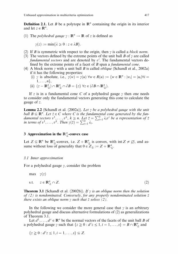
Figure 1 shows an example with two facets represented by the normal vectorsd 1 and d 2. The point z corresponds to an optimal l in (3).

Problem (3) can be reformulated as a linear programming problem in thecase that the set Z has a linear programming representation, i.e., Z ¼ fCx :Axe b; xf 0; x A Rmg, where C is an nm-matrix with Cx ¼ f ðxÞ and X ¼fx A Rm : Axe b; xf 0g is a bounded polyhedron. Then (3) can be written as

max l

s:t: 4s

i¼1

ðl� d iCxia 05Axie b5xif 0Þ

l A R: ð4Þ

As shown by Balas (1985), an equivalent linear programming representation of(4) is given by

maxXsi¼1

li

s:t: li � d iCxia 0 Ei ¼ 1; . . . ; s

Axie pib Ei ¼ 1; . . . ; s

Xsi¼1

pi ¼ 1

pib 0; xif 0; li A R Ei ¼ 1; . . . ; s: ð5Þ

From an algorithmic point of view we would like to decompose problem

Fig. 1. Inner approximation


(2) (or problem (3), respectively) into subproblems whose structure is as simpleas possible. For this purpose, let B be the unit ball of g and denote by C1; . . . ;Csand v1; . . . ; vt the fundamental cones and the fundamental vectors of BXRnf,respectively. If we denote by Ij the index set of those fundamental vectors gen-erating the cone Cj, j ¼ 1; . . . ; s, then Lemma 2.2 implies that (2) can be de-composed into s subproblems ðP jinnerÞ, j ¼ 1; . . . ; s, of the form

dj ¼ maxXi A Ij

li

s:t:Xi A Ij

livie z

lib 0 Ei A Ij

z A Z: ð6Þ

Note that each subproblem (6) has a very simple linear objective function andonly linear inequality constraints in addition to the problem dependent con-straint z A Z.

We will show in the following that, under some assumptions of non-degeneracy, each subproblem (6) generates a nondominated solution z.

Theorem 3.2. Let Z be strictly int Rne-convex, i.e. Z þ int Rne is strictly convex,and let Cj be a fundamental cone of a polyhedral gauge g. Then the optimal solu-tion of problem (6) is properly nondominated.

Proof. Let z be an optimal solution of (6). Then there exist optimal dual multi-pliers ub 0 of (6) such that z solves

maxXi A Ij

li � uXi A Ij

livi � z

0@

1A

s:t: z A Z; lib 0 Ei A Ij; ð7Þ

(see, for example, Rockafellar, 1970). We rewrite the objective function of (7)as

Xi A Ij

li � uXi A Ij

livi � z

0@

1A ¼

Xi A Ij

lið1 � uviÞ þ uz:

Since the problem is bounded it follows that ð1 � uviÞa 0 for all i A Ij (other-wise, increasing li would result in an unbounded objective value). Hence anoptimal solution of (7) satisfies li ¼ 0 whenever ð1 � uviÞ0 0, i A Ij. There-fore

Pi A Ij

lið1 � uviÞ ¼ 0 at optimality, and (7) can be replaced by

max uz

s:t: z A Z ð8Þ


with ub 0. Under the assumption that Z is strictly intRne-convex this implies

that z is indeed a properly nondominated solution. r

Note that if Z is not strictly intRne-convex, problem (6) may generate

weakly nondominated solutions since the optimal dual multiplier u used in theproof of Theorem 3.2 may have zero components. However, in the non-degenerate case that u > 0 the result of Theorem 3.2 applies also to Rn

e-convexproblems.

Corollary 3.3. Under the assumptions of Theorem 3.2, the optimal solution of(2) (or (3), respectively) is properly nondominated.

Based on the above results, an inner approximation of the nondominatedset can be constructed by iteratively solving a problem (2) (or (3), respectively).The generated solution (which is nondominated at least in the strictly intRn

e-convex case) is then added to the current approximation by including it intothe convex hull of the unit ball of the polyhedral gauge g, and a new iterationis performed with the updated g.

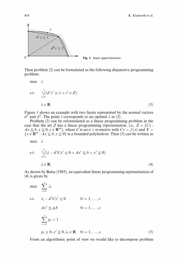
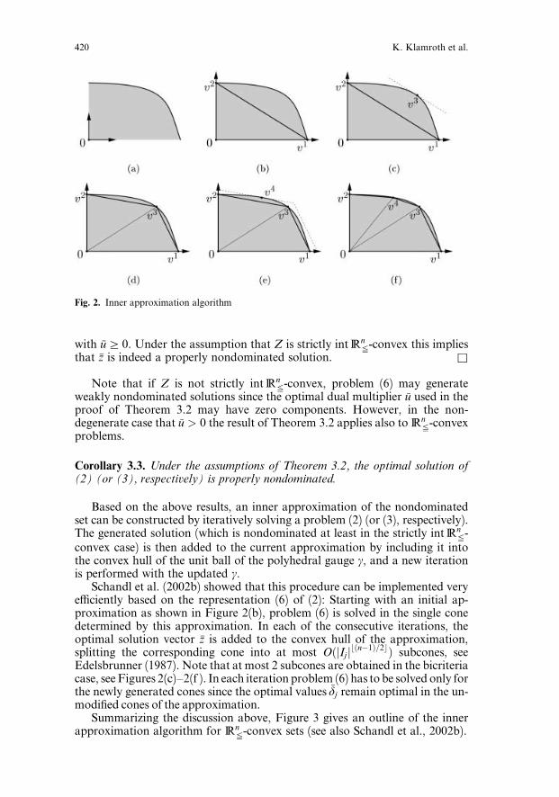
Schandl et al. (2002b) showed that this procedure can be implemented verye‰ciently based on the representation (6) of (2): Starting with an initial ap-proximation as shown in Figure 2(b), problem (6) is solved in the single conedetermined by this approximation. In each of the consecutive iterations, theoptimal solution vector z is added to the convex hull of the approximation,splitting the corresponding cone into at most OðjIj jbðn�1Þ=2cÞ subcones, seeEdelsbrunner (1987). Note that at most 2 subcones are obtained in the bicriteriacase, see Figures 2(c)–2(f ). In each iteration problem (6) has to be solved only forthe newly generated cones since the optimal values dj remain optimal in the un-modified cones of the approximation.

Summarizing the discussion above, Figure 3 gives an outline of the innerapproximation algorithm for Rn

e-convex sets (see also Schandl et al., 2002b).

Fig. 2. Inner approximation algorithm


Two di¤erent stopping criteria are implemented in the above procedurethat can be either jointly used or that can be specified separately, according todecision maker’s suggestions. Here, the value of e > 0 specifies a bound on therequired accuracy of the approximation, where the approximation error is mea-sured as jgðzÞ�1j (z denotes the next point being added in the current iteration).Thus the error is measured in a problem dependent way and using the currentapproximation in the evaluation. Alternatively, the total number of subprob-lems (6) solved during the algorithm can be bounded by specifying the maxi-mum number of cones maxConeNo to be generated during the algorithm. Notethat then maxConeNo is also an upper bound on the number of nondominatedpoints generated and added to the approximation.

The addition of new points to the convex hull of the previous approxi-mation is implemented using one iteration of the Beneath-Beyond Algorithm(see Edelsbrunner, 1987). This algorithm is among the most e‰cient convexhull algorithms (given a set S of k points in Rn, the convex hull of S is com-puted in Oðk log k þ kbðnþ1Þ=2cÞ time) and particularly well-suited for an incor-poration into the above procedure.

Summarizing the discussion above, the complexity of the inner approxi-

mation algorithm can be bounded byOðk log k þ kbðnþ1Þ=2c þ maxConeNo � TÞwhere kamaxConeNo denotes the total number of nondominated solutionsgenerating the approximation and OðTÞ is the complexity of solving (6) whichparticularly depends on the structure of the set Z.

3.2 Outer approximation

Let B be the unit ball of a polyhedral gauge g such that the fundamental vec-tors v1; . . . ; vt of BXRn

f satisfy

ðZXRnfÞJ zf 0 : ze

Xti¼1

livi;Xti¼1

li ¼ 1; lb 0

( )

Procedure: Inner Approximation

Read/generate stopping criteria: e > 0, maxConeNo;Read/generate an initial inner approximation represented by apolyhedral gauge g with unit ball B;Construct cones using the facets of B in Rn

f

for all cones doSolve (6) to find z and gðzÞ

end forwhileacones < maxConeNo and jgðnext pointÞ � 1jb e doAdd next point using the Beneath-Beyond technique;Identify new and modified conesfor all new or modified cones doSolve (6) to find z and gðzÞ

end forend whileOutput inner approximation

Fig. 3. Pseudo code of the inner approximation algorithm for an Rne-convex problem


and consider the problem

max l

s:t: lvi e zi Ei ¼ 1; . . . ; t

lb 0

zi A Z: ð9Þ

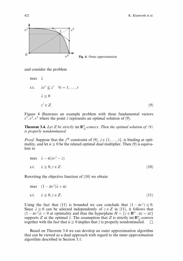
Figure 4 illustrates an example problem with three fundamental vectorsv1; v2; v3 where the point z represents an optimal solution of (9).

Theorem 3.4. Let Z be strictly intRne-convex. Then the optimal solution of (9)

is properly nondominated.

Proof. Suppose that the j th constraint of (9), j A f1; . . . ; tg, is binding at opti-mality, and let ub 0 be the related optimal dual multiplier. Then (9) is equiva-lent to

max l� uðlv j � zÞ

s:t: lb 0; z A Z: ð10Þ

Rewriting the objective function of (10) we obtain

max ð1� uv jÞlþ uz

s:t: lb 0; z A Z: ð11Þ

Using the fact that (11) is bounded we can conclude that ð1� uv jÞa 0.Since lb 0 can be selected independently of z A Z in (11), it follows thatð1� uv jÞl ¼ 0 at optimality and thus the hyperplane H ¼ fz A Rn : uz ¼ uzgsupports Z at the optimal z. The assumption that Z is strictly intRn

e-convextogether with the fact that ub 0 implies that z is properly nondominated. r

Based on Theorem 3.4 we can develop an outer approximation algorithmthat can be viewed as a dual approach with regard to the inner approximationalgorithm described in Section 3.1:

Fig. 4. Outer approximation


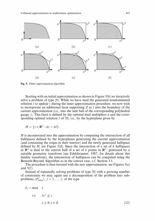
Starting with an initial approximation as shown in Figure 5(b) we iterativelysolve a problem of type (9). While we have used the generated nondominatedsolution z to update g during the inner approximation procedure, we now wishto incorporate an additional facet supporting Z at z into the boundary of thecurrent approximation (i.e., into the unit ball of the corresponding polyhedralgauge g). This facet is defined by the optimal dual multipliers u and the corre-sponding optimal solution z of (9), i.e., by the hyperplane given by

H ¼ fz A Rn : uz ¼ uzg:

H is incorporated into the approximation by computing the intersection of allhalfspaces defined by the hyperplanes generating the current approximation(and containing the origin in their interior) and the newly generated halfspacedefined by H, see Figure 5(d). Since the intersection of a set of k halfspacesin Rn is dual to the convex hull of a set of k points in Rn, generated by asuitable geometric transform (see Edelsbrunner, 1987, for details about thisduality transform), the intersection of halfspaces can be computed using theBeneath-Beyond Algorithm as in the convex case, c.f. Section 3.1.

The procedure is then iterated with the new approximation, see Figures 5(e)and 5(f ).

Instead of repeatedly solving problems of type (9) with a growing numberof constraints we may again use a decomposition of the problem into sub-problems ðP j

outerÞ, j ¼ 1; . . . ; t, of the type

dj ¼ max l

s:t: lv j e z

lb 0; z A Z: ð12Þ

Fig. 5. Outer approximation algorithm


Obviously the optimal solution of (9) can be obtained by minimizing dj overall the subproblems ðP j

outerÞ, j ¼ 1; . . . ; t, and (10) is dual to (12) for the optimalj. Since only a subset of the fundamental vectors v j changes in each iteration ofthe procedure (note that in the bicriteria case at most two new fundamentalvectors are generated in each iteration), problem (12) has to be solved only forthe newly generated fundamental vectors while the values of dj can be storedand reused for all unchanged vectors v j .

Figure 6 outlines the outer approximation algorithm for Rne-convex prob-

lems.Note that the stopping criteria used in the above algorithm correspond

exactly to those used in the inner approximation algorithm discussed in Sec-tion 3.1. Moreover, the complexity of the outer approximation algorithm cor-responds exactly to that of the inner approximation algorithm.

3.3 Simultaneous inner and outer approximation

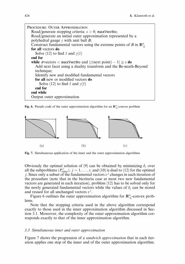
Figure 7 shows the progression of a sandwich approximation that in each iter-ation applies one step of the inner and of the outer approximation algorithm.

Procedure: Outer Approximation

Read/generate stopping criteria: e > 0, maxVecNo;Read/generate an initial outer approximation represented by apolyhedral gauge g with unit ball B;Construct fundamental vectors using the extreme points of B in Rn

f

for all vectors doSolve (12) to find z and gðzÞ

end forwhileavectors < maxVecNo and jgðnext pointÞ � 1jb e doAdd next facet using a duality transform and the Be-neath-Beyondtechnique;Identify new and modified fundamental vectorsfor all new or modified vectors doSolve (12) to find z and gðzÞ

end forend whileOutput outer approximation

Fig. 6. Pseudo code of the outer approximation algorithm for an Rne-convex problem

Fig. 7. Simultaneous application of the inner and the outer approximation algorithms


Since the nondominated set is enclosed by the two polyhedral unit balls,this approach not only allows a nice visualization of the achieved approxima-tion accuracy but also generates a set of nondominated points whose overalldistribution on the nondominated set is in general better than in each of thetwo approximations separately.

3.4 Convergence rate of the approximation for bicriteria problems

The problem of generating a piecewise linear approximation of a nondomi-nated set is closely related to the problem of approximating a convex set byan inscribed or a circumscribed polyhedron. Since the literature on polyhedralapproximations of convex sets is relatively rich (see, for example, Gruber, 1992,for an overview), in this section we use this connection to derive convergenceresults for the two algorithms described in Sections 3.1 and 3.2, concentratingon the special case of bicriteria problems (i.e., n ¼ 2).

As we have indicated, the outer approximation algorithm is closely relatedto the inner approximation algorithm by the concept of geometric duality, seeEdelsbrunner (1987). Consequently, the discussion will mainly focus on the in-ner approximation algorithm while transferring results to the case of the outerapproximation algorithm whenever it is convenient.

Wlog let the unit ball B of the current approximating gauge g be given bythe reflection set of BXRn

f, i.e., B is symmetric with respect to the origin andsatisfies

B ¼ RðBXRnfÞ :¼ fb A Rn : jbij ¼ jbij; b A ðBXRn

fÞg:

Moreover, let Z be the reflection set of ZXRnf, i.e.,

Z ¼ RðZXRnfÞ :¼ fz A Rn : jzij ¼ jzij; z A ðZXRn

fÞg:

Then the Hausdor¤ distance, dHðB;ZÞ, between the convex set Z and its poly-hedral approximation B is given by

dHðB;ZÞ ¼ supb AB

infz AZ

kz� bk2;

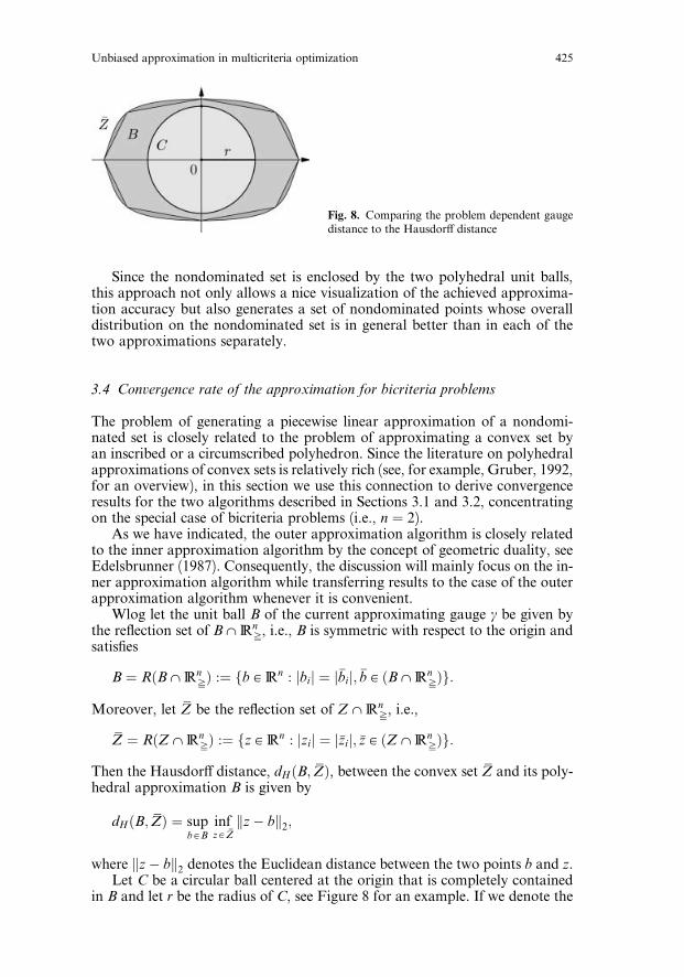
where kz� bk2 denotes the Euclidean distance between the two points b and z.Let C be a circular ball centered at the origin that is completely contained

in B and let r be the radius of C, see Figure 8 for an example. If we denote the

Fig. 8. Comparing the problem dependent gaugedistance to the Hausdor¤ distance


norm with unit ballC by k � kC , we obviously have kuk2 ¼ r � kukC for all u ARn.Moreover, kukC b gðuÞ for all u A Rn since CJB. Hence,

dHðB;ZÞ ¼ r � supb AB

infz AZ

kz� bkC

b r � supb AB

infz AZ

gðz� bÞ

¼ r � jgðzÞ � 1j;

where z is an optimal solution of (2) (or (9), respectively). Observe that theabove relations are true for the approximating gauge g and unit ball B at everyiteration of the inner as well as the outer approximation algorithm.

Rote (1992) showed that if a so-called sandwich algorithm is applied toapproximate a convex set Z in R2 by an inscribed and a circumscribed poly-hedron Pinner and Pouter, having k extreme points each (kb 4), and using thechord rule or themaximum error rule to generate the next point in each iterationof the algorithm, then the Hausdor¤ distance between the two approximatingpolyhedra can be bounded by

dHðPinner;PouterÞa8D

ðk � 2Þ2;

where D is the circumference of Z. If k approaches infinity, the value of themultiplicative constant 8 can be reduced arbitrarily close to 2p, see Rote (1992).

Since the chord rule applied in the sandwich algorithm generates the samepoints that are also found by solving problem (2), this result can be immedi-ately transferred to the inner approximation algorithm as described in Section3.1. Moreover, the maximum error rule of the sandwich algorithm applied toconvex functions generates the same points as problem (9) in the outer approx-imation algorithm if we assume that the boundary of Z is decomposed into infi-nitely small curve segments.

If we additionally use the fact that dHðPinner;PouterÞb dHðPinner;ZÞ (anddHðPinner;PouterÞb dHðZ;PouterÞ, respectively) and that in our case an approx-imation of Z is generated only in the nonnegative orthant of the coordinatesystem (the other parts of the approximating polyhedra follow by symmetry),the approximation error of the inner and the outer approximation after k iter-ations can be bounded by

jgðzÞ � 1ja 1

r� dHðB;ZÞ

¼ 1

r� dHðPinner;ZÞ

a2D

rk2; kb 4: ð13Þ

(Note that the approximation either consists of k þ 2 nondominated pointsafter k iterations, or it is exact.) Since the above bound is inversely proportional


to the radius r of the circular ball C inscribed into the final approximation, wecan try to choose C as large as possible to obtain a sharper bound. Yet anycircular ball inscribed into the initial inner approximation yields a constant rthat can be used in the above inequality and hence the inner approximation al-gorithm has a quadratic convergence rate. Note that any ball C inscribed intothe initial inner approximation can be used as a ball inscribed into the initialouter approximation so that the arguments and conclusion above are also validfor the outer approximation algorithm.

Theorem 3.5. The approximation error after k iterations of the inner approxi-mation algorithm or the outer approximation algorithm, respectively, measured

by the approximating gauge g, decreases by the order of O�1k2

�which is optimal.

Proof. The convergence rate of O�1k2

�follows directly from (13). That a qua-

dratic convergence rate is best possible for approximating a convex set inR2 byinscribed or by circumscribed polyhedra is a well known result which can beeasily verified by considering the example of a circle (see, for example, Gruber,1992). r

It may be conjectured that the convergence rate of the two approximation

algorithms if applied to problems in Rn, nb 3, is of the order O 1k2=ðn�1Þ

� �which

would be also best possible. However, corresponding results for algorithms ap-proximating convex sets inRn are – to the best knowledge of the authors – notyet available in the literature, and further research is needed in this direction.

4 Approximation in the Rne-nonconvex case

Let ZJRn be Rne-closed with intðZÞ0q, and assume without loss of gener-

ality that 0 AZe¼ZþRne.

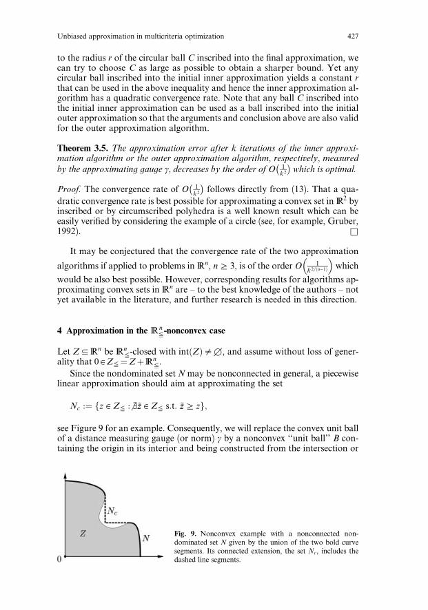
Since the nondominated set N may be nonconnected in general, a piecewiselinear approximation should aim at approximating the set

Nc :¼ fz A Ze :6 b~zz A Ze s:t: ~zzb zg;

see Figure 9 for an example. Consequently, we will replace the convex unit ballof a distance measuring gauge (or norm) g by a nonconvex ‘‘unit ball’’ B con-taining the origin in its interior and being constructed from the intersection or

Fig. 9. Nonconvex example with a nonconnected non-dominated set N given by the union of the two bold curvesegments. Its connected extension, the set Nc, includes thedashed line segments.


union of dominating cones. This unit ball is then used to define a new distancemeasuring function g as

gðzÞ :¼ minfl : z A lBg: ð14Þ

The basic idea for an approximation procedure is – similar to the convex case– to minimize the maximum g-distance between a nondominated point in Zand the boundary of B. However, while the concept of using hyperplanes andtheir corresponding normal vectors for the generation of nondominated solu-tions works well in the convex case, it has to be replaced by a suitable alterna-tive in the nonconvex case. Since the approximation itself will be constructedfrom dominating cones, it is natural to use variants of the Tchebyche¤ methodfor this purpose which theoretically allows the generation of the complete non-dominated set (Steuer and Choo, 1983; Kaliszewski, 1987).

4.1 Inner approximation

Let d 1; . . . ; d s A Rnf be a nonempty and finite set of vectors generating the non-

negative orthant, i.e., fv A Rn : v ¼Psi¼1 lid

i; lf 0g ¼ Rnf. We additionally

assume that the set B defined by

B ¼ cl Rnf

�6

i¼1;...; sðd i þ Rn

fÞ !

is bounded, has nonempty interior and that BJ ðZeXRnfÞ. Even though the

assumption of boundedness is quite restrictive in general, it will automaticallybe satisfied during all stages of the approximation algorithm that will be de-scribed at the end of this section.

Note that B could be symmetrically extended to all orthants of the coor-

dinate system, yielding a compact set BB that contains the origin in its interior.However, since we only consider points in the nonnegative orthant of the co-ordinate system, this extension has no impact on the following discussion andwe omit it for the sake of simplicity.

If we interpret the vectors d 1; . . . ; d s as local nadir points, they define a cor-responding set of local utopia points v1; . . . ; vs. The components v ji , i¼ 1; . . . ; nof these local utopia points v j, j ¼ 1; . . . ; s can be found as

vji ¼ maxfvi : vk ¼ d jk Ek0 i; k A f1; . . . ; ng; ve z; z A Zg

¼ maxfzi : zk ¼ d jk Ek0 i; k A f1; . . . ; ng; z A Zeg:

Each pair ðd j; v jÞ, j ¼ 1; . . . ; s defines an n-dimensional axis-parallel rectan-gular box which can be used to define the weights for a local application of theTchebyche¤ method. Consequently, a point v A Nc, that is currently worst ap-proximated with respect to the distance measure g and that is generated by avariation of a ‘‘local Tchebyche¤ method’’, can be determined using the follow-ing disjunctive programming problem:

max gðvÞ

s:t: 4s

i¼1ðd i þ liðvi � d iÞ ¼ v5li b 05ve zi5zi A ZÞ: ð15Þ


Within a cone d j þ Rnf, j A f1; . . . ; sg, solving (15) is equivalent to the appli-

cation of the lexicographic weighted Tchebyche¤ method with the utopia pointv j and with the weights w

ji :¼ 1

vji�d j

i

, i ¼ 1; . . . ; n, i.e., to solving

lexmin ðkv j � zkwj

y ; kv j � zk1Þ

s:t: z A Z: ð16Þ

The two problems can indeed be viewed as being equivalent since there ex-ist optimal solutions z of (16) and v; l; z j of maxfgðvÞ : d j þ lðv j � d jÞ ¼ v,lb 0; ve z j; z j A Zg such that z ¼ z j.

Moreover, problem (15) can be simplified to

max l

s:t: 4s

i¼1d i þ l v i�d i

gðv iÞ�1 e zi5zi A Z� �

lb 0: ð17Þ

In this formulation, the search directions v j � d j are normalized by the ex-

pression gðv jÞ � 1 ¼ gðv jÞ � gðd jÞ ¼ minvji�d j

i

dji

: i A f1; . . . ; ng

. Thus the dis-

tance information between the current approximation (given by B) and a pointd j þ l v j�d j

gðv jÞ�1 is captured in the value of l. In particular, the optimal solutions

v of (15) and l of (17) satisfy gðvÞ ¼ 1þ l. This is due to the fact that the op-timal v has to be located in some cone d j þ Rn

f, j A f1; . . . ; sg (note that thesame cone also contains the vector v j) and satisfies

gðvÞ ¼ g d j þ lv j � d jgðv jÞ � 1

� �

¼ g 1� l

gðv jÞ � 1

� d j þ l

gðv jÞ � 1

� v j

� �

¼ 1� l

gðv jÞ � 1

� gðd jÞ|ffl{zffl}

¼1

þ l

gðv jÞ � 1 gðv jÞ

¼ 1þ l:

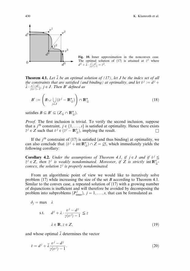
The third equality holds since d j and v j are located in the same fundamentalcone of B and thus gðad j þ bv jÞ ¼ agðd jÞ þ bgðv jÞ for all nonnegative scalarsa and b. In fact, the nonnegativity constraint in problem (17) can be relaxed dueto the defintion of the unit ball B. Figure 10 illustrates problem (17) and its op-timal solution.

Note that the disjunctive programming problem (17) has a linear program-ming reformulation if the set Z has a linear programming representation, c.f.problems (4) and (5) in Section 3.1.


Theorem 4.1. Let l be an optimal solution of (17), let J be the index set of allthe constraints that are satisfied (and binding) at optimality, and let v j :¼ d j þl v j�d j

gðv jÞ�1, j A J. Then B0 defined as

B 0 :¼ BW 6j A J

ðv j � RnfÞ

!XRn

f ð18Þ

satisfies BJB 0 J ðZeXRnfÞ.

Proof. The first inclusion is trivial. To verify the second inclusion, supposethat a j th constraint, j A f1; . . . ; sg is satisfied at optimality. Hence there existsz j A Z such that v j A ðz j � Rn

fÞ, implying the result. r

If the j th constraint of (17) is satisfied (and thus binding) at optimality, wecan also conclude that ðv j þ intRn

fÞXZ ¼ q, which immediately yields thefollowing corollary:

Corollary 4.2. Under the assumptions of Theorem 4.1, if j A J and if v j ez j A Z, then z j is weakly nondominated. Moreover, if Z is strictly intRn

e-convex, the solution z j is properly nondominated.

From an algorithmic point of view we would like to iteratively solveproblem (17) while increasing the size of the set B according to Theorem 4.1.Similar to the convex case, a repeated solution of (17) with a growing numberof disjunctions is ine‰cient and will therefore be avoided by decomposing theproblem into subproblems (P jinner), j ¼ 1; . . . ; s, that can be formulated as

dj ¼ max l

s:t: d j þ l vj � d j

gðv jÞ � 1e z

l A R; z A Z; ð19Þ

and whose optimal l determines the vector

v ¼ d j þ lv j � d jgðv jÞ � 1

: ð20Þ

Fig. 10. Inner approximation in the nonconvex case.The optimal solution of (17) is attained at z2 whered 2 þ l v2�d 2

gðv2Þ�1 ¼ z2.


Having the solution of all the subproblems (P jinner), j ¼ 1; . . . ; s available, the

optimal solution value of (17) equals the maximum value of dj which also yieldsthe related vector v as given above.

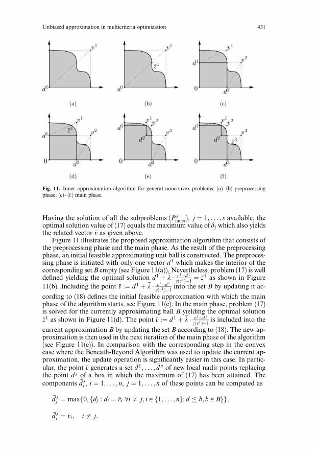
Figure 11 illustrates the proposed approximation algorithm that consists ofthe preprocessing phase and the main phase. As the result of the preprocessingphase, an initial feasible approximating unit ball is constructed. The preproces-sing phase is initiated with only one vector d 1 which makes the interior of thecorresponding set B empty (see Figure 11(a)). Nevertheless, problem (17) is welldefined yielding the optimal solution d 1 þ l v1�d 1

gðv1Þ�1 ¼ z1 as shown in Figure

11(b). Including the point v :¼ d 1 þ l v1�d 1gðv1Þ�1 into the set B by updating it ac-

cording to (18) defines the initial feasible approximation with which the mainphase of the algorithm starts, see Figure 11(c). In the main phase, problem (17)is solved for the currently approximating ball B yielding the optimal solutionz1 as shown in Figure 11(d). The point v :¼ d 1 þ l v1�d 1

gðv1Þ�1 is included into the

current approximation B by updating the set B according to (18). The new ap-proximation is then used in the next iteration of the main phase of the algorithm(see Figure 11(e)). In comparison with the corresponding step in the convexcase where the Beneath-Beyond Algorithm was used to update the current ap-proximation, the update operation is significantly easier in this case. In partic-ular, the point v generates a set d 1; . . . ; d n of new local nadir points replacingthe point d j of a box in which the maximum of (17) has been attained. Thecomponents d ji , i ¼ 1; . . . ; n, j ¼ 1; . . . ; n of these points can be computed as

djj ¼ maxf0; fdj : di ¼ vi Ei0 j; i A f1; . . . ; ng; de b; b A Bgg;

dji ¼ vi; i0 j:

Fig. 11. Inner approximation algorithm for general nonconvex problems: (a)–(b) preprocessingphase, (c)–(f ) main phase.


In the subsequent iterations, problem (19) has to be solved only in thenewly generated rectangular boxes (defined by the added local nadir and utopiapoints) while the remaining values of dj remain unchanged, see Figures 11(d)–11(f ).

As stopping criteria we can use, similar to the convex case, a bound e on therequired approximation accuracy which is again measured in a problem depen-dent way, or a bound maxBoxNo on the number of rectangular boxes that aregenerated during the algorithm. Figure 12 gives an outline of the main phase ofthe inner approximation algorithm for general nonconvex problems.

4.2 Outer approximation

Let B be defined by a nonempty and finite set of fundamental vectorsv1; . . . ; vt A Rn

b as

B ¼ RnfX 6

i¼1;...; tðvi � Rn

fÞ

and let ðZeXRnfÞJB. Note that the set B is always closed and bounded.

Moreover, since B as defined above encloses the unit ball used in the inner ap-proximation, independently of the choice of the vectors d 1; . . . ; d s (inner ap-proximation) and v1; . . . ; vt (outer approximation), the corresponding distancemeasure g used in the outer approximation is always a lower bound on thatused in the inner approximation.

Analogously to the inner approximation approach, we can interpret thevectors v1; . . . ; vt as local utopia points defining a corresponding set of local

nadir points d 1; . . . ; d t and thereby the desired Tchebyche¤ boxes. Even though

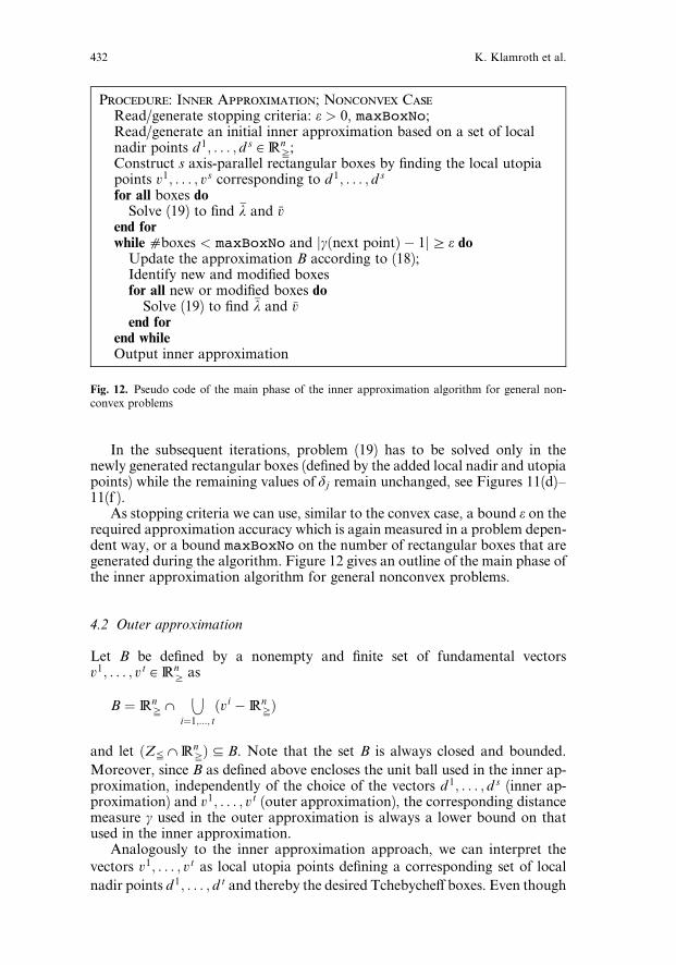
Procedure: Inner Approximation; Nonconvex CaseRead/generate stopping criteria: e > 0, maxBoxNo;Read/generate an initial inner approximation based on a set of localnadir points d 1; . . . ; d s A Rn

f;Construct s axis-parallel rectangular boxes by finding the local utopiapoints v1; . . . ; vs corresponding to d 1; . . . ; d s

for all boxes doSolve (19) to find l and v

end forwhileaboxes < maxBoxNo and jgðnext pointÞ � 1jb e doUpdate the approximation B according to (18);Identify new and modified boxesfor all new or modified boxes doSolve (19) to find l and v

end forend whileOutput inner approximation

Fig. 12. Pseudo code of the main phase of the inner approximation algorithm for general non-convex problems


the concept of nadir points is not unique for higher dimensional problems, wecan use the symmetry to the inner approximation approach and compute thecomponents d j

i , i ¼ 1; . . . ; n of local nadir points d j, j ¼ 1; . . . ; t as

dji ¼ maxfdi : dk ¼ v

jk Ek0 i; k A f1; . . . ; ng; d e z; z A Zg

¼ maxfzi : zk ¼ vjk Ek0 i; k A f1; . . . ; ng; z A Zeg:

Using this definition, each pair ðd j; v jÞ, j ¼ 1; . . . ; t again defines an n-dimensional axis-parallel rectangular box and thus the weights needed for theTchebyche¤ method. Consequently, the disjunctive programming problems(15) and (17) can also be applied in the case of an outer approximation sincethese programs are solely based on pairs of local nadir and utopia points. How-ever, since the current approximation (given by B) encloses the set ZeXRn

f,

the orientation of the search direction as well as its normalization as used in(17) have to be adapted to the new situation. This leads to the following vari-ation of (17) in which the nonnegativity constraint for l can also be relaxed:

min l

s:t: 4s

i¼1

vi � l � vi � d i

1 � gðd iÞ e zi5zi A Z

� �

l A R: ð21Þ

Note that the search within each of the cones d j þ Rnf is now initiated at the

point v j, outside the set ZeXRnf, and thus the search is directed ‘‘inward’’.

The normalization term can be evaluated as 1 � gðd jÞ ¼ gðv jÞ � gðd jÞ ¼

minvji�d j

i

vj

i

: i A f1; . . . ; ng� �

. A similar analysis as in Section 4.1 shows that the

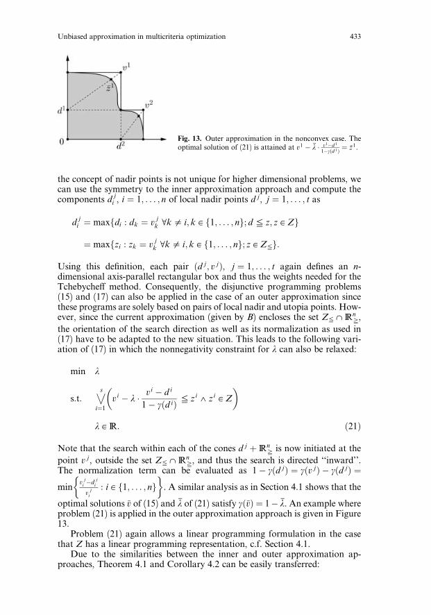
optimal solutions v of (15) and l of (21) satisfy gðvÞ ¼ 1� l. An example whereproblem (21) is applied in the outer approximation approach is given in Figure13.

Problem (21) again allows a linear programming formulation in the casethat Z has a linear programming representation, c.f. Section 4.1.

Due to the similarities between the inner and outer approximation ap-proaches, Theorem 4.1 and Corollary 4.2 can be easily transferred:

Fig. 13. Outer approximation in the nonconvex case. Theoptimal solution of (21) is attained at v1 � l � v1�d 1

1�gðd 1Þ ¼ z1.


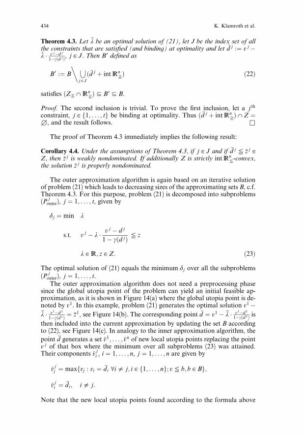
Theorem 4.3. Let l be an optimal solution of (21), let J be the index set of allthe constraints that are satisfied (and binding) at optimality and let d j :¼ v j �l � v j�d j

1�gðd jÞ, j A J. Then B 0 defined as

B 0 :¼ B

�6j A J

ðd j þ int RnfÞ ð22Þ

satisfies ðZeXRnfÞJB 0 JB.

Proof. The second inclusion is trivial. To prove the first inclusion, let a j th

constraint, j A f1; . . . ; tg be binding at optimality. Thus ðd j þ int RnfÞXZ ¼

q, and the result follows. r

The proof of Theorem 4.3 immediately implies the following result:

Corollary 4.4. Under the assumptions of Theorem 4.3, if j A J and if d j e z j AZ, then z j is weakly nondominated. If additionally Z is strictly int Rn

e-convex,the solution z j is properly nondominated.

The outer approximation algorithm is again based on an iterative solutionof problem (21) which leads to decreasing sizes of the approximating sets B, c.f.Theorem 4.3. For this purpose, problem (21) is decomposed into subproblems(P

jouter), j ¼ 1; . . . ; t, given by

dj ¼ min l

s:t: v j � l � v j � d j

1 � gðd jÞ e z

l A R; z A Z: ð23Þ

The optimal solution of (21) equals the minimum dj over all the subproblems(P

jouter), j ¼ 1; . . . ; t.The outer approximation algorithm does not need a preprocessing phase

since the global utopia point of the problem can yield an initial feasible ap-proximation, as it is shown in Figure 14(a) where the global utopia point is de-noted by v1. In this example, problem (21) generates the optimal solution v1 �l � v1�d 1

1�gðd 1Þ ¼ z1, see Figure 14(b). The corresponding point d ¼ v1 � l � v1�d 1

1�gðd 1Þ is

then included into the current approximation by updating the set B accordingto (22), see Figure 14(c). In analogy to the inner approximation algorithm, the

point d generates a set v1; . . . ; vn of new local utopia points replacing the pointv j of that box where the minimum over all subproblems (23) was attained.Their components v ji , i ¼ 1; . . . ; n, j ¼ 1; . . . ; n are given by

vjj ¼ maxfvj : vi ¼ di Ei0 j; i A f1; . . . ; ng; ve b; b A Bg;

vji ¼ di; i0 j:

Note that the new local utopia points found according to the formula above


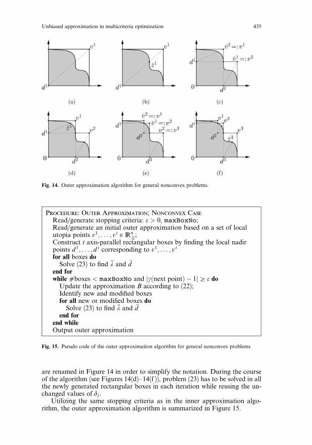
are renamed in Figure 14 in order to simplify the notation. During the courseof the algorithm (see Figures 14(d)–14(f )), problem (23) has to be solved in allthe newly generated rectangular boxes in each iteration while reusing the un-changed values of dj.

Utilizing the same stopping criteria as in the inner approximation algo-rithm, the outer approximation algorithm is summarized in Figure 15.

Procedure: Outer Approximation; Nonconvex Case

Read/generate stopping criteria: e > 0, maxBoxNo;Read/generate an initial outer approximation based on a set of localutopia points v1; . . . ; vt A Rn

f;Construct t axis-parallel rectangular boxes by finding the local nadirpoints d 1; . . . ; d t corresponding to v1; . . . ; vt

for all boxes doSolve (23) to find l and d

end forwhileaboxes < maxBoxNo and jgðnext pointÞ � 1jb e do

Update the approximation B according to (22);Identify new and modified boxesfor all new or modified boxes do

Solve (23) to find l and dend for

end whileOutput outer approximation

Fig. 14. Outer approximation algorithm for general nonconvex problems.

Fig. 15. Pseudo code of the outer approximation algorithm for general nonconvex problems


4.3 Simultaneous inner and outer approximation in the Rne-nonconvex case

Even though Figures 11 and 14 suggest that the pairs of local nadir andutopia points generating the approximating boxes in the inner as well as in theouter approximation approach coincide if both algorithms are initialized ac-cordingly, this is not true in general for two reasons: On one hand, the distancemeasure g and the approximation B di¤er between the two algorithms and dif-ferent boxes may contain the optimal solution of (17) and (21), respectively. Onthe other hand, the new local nadir and utopia points computed within one it-eration of the procedure may not coincide in higher dimensional problems, afact that immediately leads to di¤erent approximations. This indicates that acombination of the two procedures may be beneficial also for nonconvex prob-lems.

5 Conclusions

In this paper we have developed inner as well as outer approximation algo-rithms that generate piecewise linear approximations of the nondominated setof convex and nonconvex multicriteria programs. In all cases, the approxima-tion itself is used to define a problem dependent distance measure, leading tounbiased and scale-independent approximations. Moreover, the approxima-tion is always improved where it is needed most, that is, where the current ap-proximation error is maximal. This self-correcting property of the approxima-tion was not present in the algorithms proposed for the nonconvex problems inSchandl et al. (2002b) and is a significant improvement.

The algorithms limit the involvement of the decision maker only to the ini-tialization when the starting approximation has to be given. If such an interac-tion was desirable while approximation is being constructed, the algorithmscould be easily modified. The authors however believe that decision makersmay appreciate an interaction-free approximating technique releasing themfrom interrogation and queries.

A byproduct of the developed algorithms are the new scalarization tech-niques for generating (weakly) nondominated points. These techniques searchthe objective space by means of properly defined directions.

While quadratic convergence of the developed algorithms is proven forconvex bicriteria problems, similar results can only be conjectured for the mul-ticriteria case. Future research should focus, among others, on convergence re-sults under more general assumptions as well as practical studies and compar-isons of the proposed algorithms with other approximation approaches.

References

Balas E (1985) Disjunctive programming and a hierarchy of relaxations for discrete optimizationproblems. SIAM J. Algebraic Discrete Methods 6:466–486

Belov YA, Shafranskii SV (1991) Application of a di¤erentiable family of convolutions in the so-lution of problems of multicriterial optimization. Dokl. Akad. Nauk Ukrain. SSR 163:49–52.Russian

Benson HP, Sayin S (1997) Towards finding global representations of the e‰cient set in multipleobjective mathematical programming. Naval Research Logistics 44:47–67

Czyzak P, Jaszkiewicz A (1998) Pareto simulated annealing – a metaheuristic technique for multi-ple-objective combinatorial optimization. Journal of Multi-Criteria Decision Analysis 7:34–47


Das I (1999) An improved technique for choosing parameters for Pareto surface generation usingnormal-boundary intersection. In: Short Paper Proceedings of the Third World Congress ofStructural and Multidisciplinary Optimization 2:411–413

Deb K (2001) Multi-objective optimization using evolutionary algorithms. John Wiley & SonsLtd., Chichester, England

Edelsbrunner H (1987) Algorithms in combinatorial geometry. Springer-Verlag, BerlinGalperin EA, Wiecek MM (1999) Retrieval and use of the balance set in multiobjective global

optimization. Computers and Mathematics with Applications 37:111–123Gandibleux X, Mezdaoui N, Freville A (1997) A tabu search procedure to solve multiobjective

combinatorial optimization problems. In: Caballero R, Ruiz F, Steuer RE (eds) Advances inMultiple Objective and Goal Programming, pp. 291–300. Springer-Verlag, Berlin

Geo¤rion AM (1968) Proper e‰ciency and the theory of vector maximization. Journal of Math-ematical Analysis and Applications 22(3):618–630

Gruber PM (1992) Approximation of convex bodies. In: Gruber PM, Wills JM (eds) Handbook ofConvex Geometry, pp. 321–345. North-Holland, Amsterdam

Helbig S (1991) Approximation of the e‰cient set by perturbation of the ordering cone. ZOR –Methods and Models of Operations Research 35:197–220

Kaliszewski I (1987) A modified weighted Tchebyche¤ metric for multiple objective program-ming. Computers and Operations Research 14:315–323

Kaliszewski I (1994) Quantitative Pareto analysis by cone separation technique. Kluwer AcademicPublishers, Dordrecht

Kostreva MM, Zheng Q, Zhuang D (1995) A method for approximating solutions of multicriterianonlinear optimization problems. Optimization Methods and Software 5:209–226

Lemaire B (1992) Approximation in multiobjective optimization. Journal of Global Optimization2:117–132

Minkowski H. Gesammelte Abhandlungen, Band 2. In: Hilbert D (ed) Teubner Verlag, Leipzigund Berlin (1911). Also in: Chelsea Publishing Company, New York, 1967

Nefedov VN (1984) On the approximation of a Pareto set. U.S.S.R. Computational Mathematicsand Mathematical Physics 24(4):19–28

Popov NM (1982) Approximation of a Pareto set by the convolutions method. Vestnik Moskov.Univ. Ser. XV Vychisl. Mat. Kibernet 81:35–41. Russian

Rockafellar RT (1970) Convex analysis. Princeton University Press, Princeton, NJRote G (1992) The convergence rate of the sandwich algorithm for approximating convex func-

tions. Computing 48:337–361Schandl B (1999) Norm-based evaluation and approximation in multicriteria programming.

Ph.D. thesis, Clemson University, Clemson, SC. Available at http://www.math.clemson.edu/a¤ordability/publications.html (15.12.1999)

Schandl B, Klamroth K, Wiecek MM (2001) Norm-based approximation in bicriteria program-ming. Computational Optimization and Applications 20:23–42

Schandl B, Klamroth K, Wiecek MM (2002a) Introducing oblique norms into multiple criteriaprogramming. Journal of Global Optimization 23:81–97

Schandl B, Klamroth K, Wiecek MM (2002b) Norm-based approximation in multicriteria pro-gramming. Computers and Mathematics with Applications. To appear

Smirnov MM (1996) On a logical convolution of a criterion vector in the Pareto set approxima-tion problem. Computational Mathematics and Mathematical Physics 36:605–614

Sobol’ IM, Levitan YL (1997) Error estimates for the crude approximation of the trade-o¤ curve.In: Fandel G, Gal T (eds) Multiple Criteria Decision Making, pp. 83–92. Springer-Verlag,Berlin

Statnikov RB, Matusov JB (1996) Use of Pt-nets for the approximation of the Edgeworth-Paretoset in multicriteria optimization. Journal of Optimization Theory and Applications 91:543–560

Steuer RE, Choo EU (1983) An interactive weighted Tchebyche¤ procedure for multiple objectiveprogramming. Mathematical Programming 26:326–344

Ulungu EL, Teghem J, Fortemps PH, Tuyttens D (1999) MOSA method: A tool for solving mul-tiobjective combinatorial optimization problems. Journal of Multi-Criteria Decision Analysis8:221–236

Zitzler E, Deb K, Thiele L, Coello CA, Cotne D (2001) Evolutionary multi-criterion optimization.Volume 1993 of Lecture Notes in Computer Science. Springer-Verlag, Berlin


unbiased approximation in multicriteria optimization

Documents