unbiased recursive partitioning: a conditional inference...

Unbiased Recursive Partitioning: A Conditional

Inference Framework

Torsten HothornFriedrich-Alexander-Universitat

Erlangen-Nurnberg,

Kurt HornikWirtschaftsuniversitat Wien

Achim ZeileisWirtschaftsuniversitat Wien

Abstract

Recursive binary partitioning is a popular tool for regression analysis. Two fundamentalproblems of exhaustive search procedures usually applied to fit such models have been knownfor a long time: overfitting and a selection bias towards covariates with many possible splitsor missing values. While pruning procedures are able to solve the overfitting problem, thevariable selection bias still seriously affects the interpretability of tree-structured regressionmodels. For some special cases unbiased procedures have been suggested, however lacking acommon theoretical foundation. We propose a unified framework for recursive partitioningwhich embeds tree-structured regression models into a well defined theory of conditionalinference procedures. Stopping criteria based on multiple test procedures are implemented andit is shown that the predictive performance of the resulting trees is as good as the performanceof established exhaustive search procedures. It turns out that the partitions and thereforethe models induced by both approaches are structurally different, confirming the need for anunbiased variable selection. Moreover, it is shown that the prediction accuracy of trees withearly stopping is equivalent to the prediction accuracy of pruned trees with unbiased variableselection. The methodology presented here is applicable to all kinds of regression problems,including nominal, ordinal, numeric, censored as well as multivariate response variables andarbitrary measurement scales of the covariates. Data from studies on glaucoma classification,node positive breast cancer survival and mammography experience are re-analyzed.

Keywords: permutation tests, variable selection, multiple testing, ordinal regression trees, multi-variate regression trees.

1. Introduction

Statistical models that regress the distribution of a response variable on the status of multiplecovariates are tools for handling two major problems in applied research: prediction and expla-nation. The function space represented by regression models focusing on the prediction problemmay be arbitrarily complex; indeed, ‘black box’ systems like support vector machines or ensemblemethods are excellent predictors. In contrast, regression models appropriate for gaining insightinto the mechanism of the data generating process are required to offer a human readable repre-sentation. Generalized linear models or the Cox model are representatives of regression modelswhere parameter estimates of the coefficients and their distribution are used to judge the relevanceof single covariates.

With their seminal work on automated interaction detection (AID), Morgan and Sonquist (1963)introduced another class of simple regression models for prediction and explanation nowadaysknown as ‘recursive partitioning’ or ‘trees’. Many variants and extensions have been published inthe last 40 years, the majority of which are special cases of a simple two-stage algorithm: firstpartition the observations by univariate splits in a recursive way and second fit a constant modelin each cell of the resulting partition. The most popular implementations of such algorithms are‘CART’ (Breiman, Friedman, Olshen, and Stone 1984) and ‘C4.5’ (Quinlan 1993). Not unlike AID,both perform an exhaustive search over all possible splits maximizing an information measure of

This is a preprint of an article published in Journal of Computational and Graphical Statistics,Volume 15, Number 3, Pages 651–674. Copyright c© 2006 American Statistical Association,Institute of Mathematical Statistics, and Interface Foundation of North America

2 Unbiased Recursive Partitioning: A Conditional Inference Framework

node impurity selecting the covariate showing the best split. This approach has two fundamentalproblems: overfitting and a selection bias towards covariates with many possible splits. Withrespect to the overfitting problem Mingers (1987) notes that the algorithm

[. . . ] has no concept of statistical significance, and so cannot distinguish between asignificant and an insignificant improvement in the information measure.

Within the exhaustive search framework, pruning procedures, mostly based on some form ofcross-validation, are necessary to restrict the number of cells in the resulting partitions in orderto avoid overfitting problems. While pruning is successful in selecting the right-sized tree, theinterpretation of the trees is affected by the biased variable selection. This bias is induced bymaximizing a splitting criterion over all possible splits simultaneously and was identified as aproblem by many researchers (e.g., Kass 1980; Segal 1988; Breiman et al. 1984, p. 42). The natureof the variable selection problem under different circumstances has been studied intensively (Whiteand Liu 1994; Jensen and Cohen 2000; Shih 2004) and Kim and Loh (2001) argue that exhaustivesearch methods are biased towards variables with many missing values as well. With this articlewe enter at the point where White and Liu (1994) demand for

[. . . ] a statistical approach [to recursive partitioning] which takes into account thedistributional properties of the measures.

We present a unified framework embedding recursive binary partitioning with piecewise constantfits into the well-defined theory of permutation tests developed by Strasser and Weber (1999). Theconditional distribution of statistics measuring the association between responses and covariatesis the basis for an unbiased selection among covariates measured at different scales. Moreover,multiple test procedures are applied to determine whether no significant association between anyof the covariates and the response can be stated and the recursion needs to stop. We show thatsuch statistically motivated stopping criteria implemented via hypothesis tests lead to regressionmodels whose predictive performance is equivalent to the performance of optimally pruned trees,therefore offering an intuitive and computationally efficient solution to the overfitting problem.The development of the framework presented here was inspired by various attempts to solve boththe overfitting and variable selection problem published in the last 25 years (a far more detailedoverview is given by Murthy 1998). The χ2 automated interaction detection algorithm (‘CHAID’,Kass 1980) is the first approach based on statistical significance tests for contingency tables. Thebasic idea of this algorithm is the separation of the variable selection and splitting procedure. Thesignificance of the association between a nominal response and one of the covariates is investigatedby a χ2 test and the covariate with highest association is selected for splitting. Consequently, thisalgorithm has a concept of statistical significance and a criterion to stop the algorithm can easilybe implemented based on formal hypothesis tests.A series of papers aiming at unbiased recursive partitioning for nominal and continuous responsesstarts with ‘FACT’ (Loh and Vanichsetakul 1988), where covariates are selected within an analysisof variance (ANOVA) framework treating a nominal response as the independent variable. Basi-cally, the covariate with largest F -ratio is selected for splitting. Nominal covariates are coerced toordered variables via the canonical variate of the corresponding matrix of dummy codings. Thisinduces a biased variable selection when nominal covariates are present and therefore ‘QUEST’(Loh and Shih 1997) addresses this problem by selecting covariates on a P -value scale. For contin-uous variables, P -values are derived from the corresponding ANOVA F -statistics and for nominalcovariates a χ2 test is applied. This approach reduces the variable selection bias substantially.Further methodological developments within this framework include the incorporation of a lineardiscriminant analysis model within each node of a tree (Kim and Loh 2003) and multiway splits(‘CRUISE’, Kim and Loh 2001). For continuous responses, ‘GUIDE’ (Loh 2002) seeks to implementunbiasedness by a different approach. Here, the association between the sign of model residualsand each covariate is measured by a P -value derived from a χ2 test. Continuous covariates arecategorized to four levels prior to variable selection; however, models are fitted to untransformed

Copyright c© 2006 American Statistical Association, Institute of Mathematical Statistics, and InterfaceFoundation of North America

Torsten Hothorn, Kurt Hornik, Achim Zeileis 3

covariates in the nodes. These approaches are already very successful in reducing the variableselection bias and typically perform very well in the partitioning tasks they were designed for.Building on these ideas, we introduce a new unifying conceptual framework for unbiased recursivepartitioning based on conditional hypothesis testing that, in addition to models for continuous andcategorical data, includes procedures applicable to censored, ordinal or multivariate responses.

Previous attempts to implement permutation (or randomization) tests in recursive partitioningalgorithms aimed at solving the variable selection and overfitting problem (Jensen and Cohen2000), however focusing on special situations only. Resampling procedures have been employed forassessing split statistics for censored responses by LeBlanc and Crowley (1993). Frank and Witten(1998) utilize the conditional Monte-Carlo approach for the approximation of the distribution ofFisher’s exact test for nominal responses and the conditional probability of an observed contingencytable is used by Martin (1997). The asymptotic distribution of a 2×2 table obtained by maximizingthe χ2 statistic over possible splits in a continuous covariate is derived by Miller and Siegmund(1982). Maximally selected rank statistics (Lausen and Schumacher 1992) can be applied tocontinuous and censored responses as well and are applied to correct the bias of exhaustive searchrecursive partitioning by Lausen, Hothorn, Bretz, and Schumacher (2004). An approximation tothe distribution of the Gini criterion is given by Dobra and Gehrke (2001). However, lackingsolutions for more general situations, these auspicious approaches are hardly ever applied and themajority of tree-structured regression models reported and interpreted in applied research papersis biased. The main reason is that computationally efficient solutions are available for special casesonly.

The framework presented in Section 3 is efficiently applicable to regression problems where bothresponse and covariates can be measured at arbitrary scales, including nominal, ordinal, discreteand continuous as well as censored and multivariate variables. The treatment of special situationsis explained in Section 4 and applications including glaucoma classification, node positive breastcancer survival and a questionnaire on mammography experience illustrate the methodology inSection 5. Finally, we show by benchmarking experiments that recursive partitioning based on sta-tistical criteria as introduced in this paper lead to regression models whose predictive performanceis as good as the performance of optimally pruned trees.

2. Recursive binary partitioning

We focus on regression models describing the conditional distribution of a response variable Ygiven the status of m covariates by means of tree-structured recursive partitioning. The responseY from some sample space Y may be multivariate as well. The m-dimensional covariate vectorX = (X1, . . . , Xm) is taken from a sample space X = X1 × · · · × Xm. Both response variableand covariates may be measured at arbitrary scales. We assume that the conditional distributionD(Y|X) of the response Y given the covariates X depends on a function f of the covariates

D(Y|X) = D(Y|X1, . . . , Xm) = D(Y|f(X1, . . . , Xm)),

where we restrict ourselves to partition based regression relationships, i.e., r disjoint cells B1, . . . , Br

partitioning the covariate space X =⋃r

k=1 Bk. A model of the regression relationship is to befitted based on a learning sample Ln, i.e., a random sample of n independent and identicallydistributed observations, possibly with some covariates Xji missing,

Ln = {(Yi, X1i, . . . , Xmi); i = 1, . . . , n}.

A generic algorithm for recursive binary partitioning for a given learning sample Ln can be for-mulated using non-negative integer valued case weights w = (w1, . . . , wn). Each node of a tree isrepresented by a vector of case weights having non-zero elements when the corresponding observa-tions are elements of the node and are zero otherwise. The following generic algorithm implementsrecursive binary partitioning:

Copyright c© 2006 American Statistical Association, Institute of Mathematical Statistics, and Interface

Foundation of North America


1. For case weights w test the global null hypothesis of independence between any of the mcovariates and the response. Stop if this hypothesis cannot be rejected. Otherwise select thej∗th covariate Xj∗ with strongest association to Y.

2. Choose a set A∗ ⊂ Xj∗ in order to split Xj∗ into two disjoint sets A∗ and Xj∗ \ A∗. Thecase weights wleft and wright determine the two subgroups with wleft,i = wiI(Xj∗i ∈ A∗)and wright,i = wiI(Xj∗i 6∈ A∗) for all i = 1, . . . , n (I(·) denotes the indicator function).

3. Recursively repeat steps 1 and 2 with modified case weights wleft and wright, respectively.

As we sketched in the introduction, the separation of variable selection and splitting procedureinto steps 1 and 2 of the algorithm is the key for the construction of interpretable tree structuresnot suffering a systematic tendency towards covariates with many possible splits or many missingvalues. In addition, a statistically motivated and intuitive stopping criterion can be implemented:We stop when the global null hypothesis of independence between the response and any of the mcovariates cannot be rejected at a pre-specified nominal level α. The algorithm induces a partition{B1, . . . , Br} of the covariate space X , where each cell B ∈ {B1, . . . , Br} is associated with avector of case weights.

3. Recursive partitioning by conditional inference

In the main part of this section we focus on step 1 of the generic algorithm. Unified tests forindependence are constructed by means of the conditional distribution of linear statistics in thepermutation test framework developed by Strasser and Weber (1999). The determination of thebest binary split in one selected covariate and the handling of missing values is performed basedon standardized linear statistics within the same framework as well.

Variable selection and stopping criteria

At step 1 of the generic algorithm given in Section 2 we face an independence problem. We needto decide whether there is any information about the response variable covered by any of the mcovariates. In each node identified by case weights w, the global hypothesis of independence isformulated in terms of the m partial hypotheses Hj

0 : D(Y|Xj) = D(Y) with global null hypothesisH0 =

⋂mj=1 Hj

0 . When we are not able to reject H0 at a pre-specified level α, we stop the recursion.If the global hypothesis can be rejected, we measure the association between Y and each of thecovariates Xj , j = 1, . . . ,m, by test statistics or P -values indicating the deviation from the partialhypotheses Hj

0 .For notational convenience and without loss of generality we assume that the case weights wi areeither zero or one. The symmetric group of all permutations of the elements of (1, . . . , n) withcorresponding case weights wi = 1 is denoted by S(Ln,w). A more general notation is given inAppendix A. We measure the association between Y and Xj , j = 1, . . . ,m, by linear statistics ofthe form

Tj(Ln,w) = vec

(n∑

i=1

wigj(Xji)h(Yi, (Y1, . . . ,Yn))>)∈ Rpjq (1)

where gj : Xj → Rpj is a non-random transformation of the covariate Xj . The influence functionh : Y×Yn → Rq depends on the responses (Y1, . . . ,Yn) in a permutation symmetric way. Section 4explains how to choose gj and h in different practical settings. A pj × q matrix is converted intoa pjq column vector by column-wise combination using the ‘vec’ operator.

The distribution of Tj(Ln,w) under Hj0 depends on the joint distribution of Y and Xj , which

is unknown under almost all practical circumstances. At least under the null hypothesis one candispose of this dependency by fixing the covariates and conditioning on all possible permutations ofthe responses. This principle leads to test procedures known as permutation tests. The conditional



expectation µj ∈ Rpjq and covariance Σj ∈ Rpjq×pjq of Tj(Ln,w) under H0 given all permutationsσ ∈ S(Ln,w) of the responses are derived by Strasser and Weber (1999):

µj = E(Tj(Ln,w)|S(Ln,w)) = vec

((n∑

i=1

wigj(Xji)

)E(h|S(Ln,w))>

),

Σj = V(Tj(Ln,w)|S(Ln,w))

=w·

w· − 1V(h|S(Ln,w))⊗

(∑i

wigj(Xji)⊗ wigj(Xji)>)

(2)

− 1w· − 1

V(h|S(Ln,w))⊗

(∑i

wigj(Xji)

)⊗

(∑i

wigj(Xji)

)>

where w· =∑n

i=1 wi denotes the sum of the case weights, ⊗ is the Kronecker product and theconditional expectation of the influence function is

E(h|S(Ln,w)) = w−1·

∑i

wih(Yi, (Y1, . . . ,Yn)) ∈ Rq

with corresponding q × q covariance matrix

V(h|S(Ln,w)) = w−1·

∑i

wi (h(Yi, (Y1, . . . ,Yn))− E(h|S(Ln,w)))

(h(Yi, (Y1, . . . ,Yn))− E(h|S(Ln,w)))> .

Having the conditional expectation and covariance at hand we are able to standardize a linearstatistic T ∈ Rpq of the form (1) for some p ∈ {p1, . . . , pm}. Univariate test statistics c mappingan observed multivariate linear statistic t ∈ Rpq into the real line can be of arbitrary form. Anobvious choice is the maximum of the absolute values of the standardized linear statistic

cmax(t, µ,Σ) = maxk=1,...,pq

∣∣∣∣∣ (t− µ)k√(Σ)kk

∣∣∣∣∣utilizing the conditional expectation µ and covariance matrix Σ. The application of a quadraticform cquad(t, µ,Σ) = (t−µ)Σ+(t−µ)> is one alternative, although computationally more expensivebecause the Moore-Penrose inverse Σ+ of Σ is involved. It is important to note that the teststatistics c(tj , µj ,Σj), j = 1, . . . ,m, cannot be directly compared in an unbiased way unless allof the covariates are measured at the same scale, i.e., p1 = pj , j = 2, . . . ,m. In order to allowfor an unbiased variable selection we need to switch to the P -value scale because P -values forthe conditional distribution of test statistics c(Tj(Ln,w), µj ,Σj) can be directly compared amongcovariates measured at different scales. In step 1 of the generic algorithm we select the covariatewith minimum P -value, i.e., the covariate Xj∗ with j∗ = argminj=1,...,m Pj , where

Pj = PHj0(c(Tj(Ln,w), µj ,Σj) ≥ c(tj , µj ,Σj)|S(Ln,w))

denotes the P -value of the conditional test for Hj0 .

So far, we have only addressed testing each partial hypothesis Hj0 , which is sufficient for an unbiased

variable selection. A global test for H0 required in step 1 can be constructed via an aggregationof the transformations gj , j = 1, . . . ,m, i.e., using a linear statistic of the form

T(Ln,w) = vec

(n∑

i=1

wi

(g1(X1i)>, . . . , gm(Xmi)>

)>h(Yi, (Y1, . . . ,Yn))>

).




However, this approach is less attractive for learning samples with missing values. Universally ap-plicable approaches are multiple test procedures based on P1, . . . , Pm. Simple Bonferroni-adjustedP -values or a min-P -value resampling approach are just examples and we refer to the multipletesting literature (e.g., Westfall and Young 1993) for more advanced methods. We reject H0 whenthe minimum of the adjusted P -values is less than a pre-specified nominal level α and otherwisestop the algorithm. In this sense, α may be seen as a unique parameter determining the size ofthe resulting trees.The conditional distribution and thus the P -value of the statistic c(t, µ,Σ) can be computed inseveral different ways (see Hothorn, Hornik, van de Wiel, and Zeileis 2006, for an overview). Forsome special forms of the linear statistic, the exact distribution of the test statistic is tractable;conditional Monte-Carlo procedures can always be used to approximate the exact distribution.Strasser and Weber (1999) proved (Theorem 2.3) that the conditional distribution of linear statis-tics T with conditional expectation µ and covariance Σ tends to a multivariate normal distributionwith parameters µ and Σ as n,w· → ∞. Thus, the asymptotic conditional distribution of teststatistics of the form cmax is normal and can be computed directly in the univariate case (pjq = 1)or approximated by means of quasi-randomized Monte-Carlo procedures in the multivariate setting(Genz 1992). Quadratic forms cquad follow a asymptotic χ2 distribution with degrees of freedomgiven by the rank of Σ (Theorem 6.20, Rasch 1995), and therefore asymptotic P -values can becomputed efficiently.

Splitting criteria

Once we have selected a covariate in step 1 of the algorithm, the split itself can be established by anysplitting criterion, including those established by Breiman et al. (1984) or Shih (1999). Instead ofsimple binary splits, multiway splits can be implemented as well, for example utilizing the work ofO’Brien (2004). However, most splitting criteria are not applicable to response variables measuredat arbitrary scales and we therefore utilize the permutation test framework described above tofind the optimal binary split in one selected covariate Xj∗ in step 2 of the generic algorithm. Thegoodness of a split is evaluated by two-sample linear statistics which are special cases of the linearstatistic (1). For all possible subsets A of the sample space Xj∗ the linear statistic

TAj∗(Ln,w) = vec

(n∑

i=1

wiI(Xj∗i ∈ A)h(Yi, (Y1, . . . ,Yn))>)∈ Rq

induces a two-sample statistic measuring the discrepancy between the samples {Yi|wi > 0 and Xji ∈A; i = 1, . . . , n} and {Yi|wi > 0 and Xji 6∈ A; i = 1, . . . , n}. The conditional expectation µA

j∗ andcovariance ΣA

j∗ can be computed by (2). The split A∗ with a test statistic maximized over allpossible subsets A is established:

A∗ = argmaxA

c(tAj∗ , µ

Aj∗ ,Σ

Aj∗). (3)

Note that we do not need to compute the distribution of c(tAj∗ , µ

Aj∗ ,Σ

Aj∗) in step 2. In order to

prevent pathological splits one can restrict the number of possible subsets that are evaluated, forexample by introducing restrictions on the sample size or the sum of the case weights in each ofthe two groups of observations induced by a possible split.

Missing values and surrogate splits

If an observation Xji in covariate Xj is missing, we set the corresponding case weight wi to zerofor the computation of Tj(Ln,w) and, if we would like to split in Xj , in TA

j (Ln,w) as well. Oncea split A∗ in Xj has been implemented, surrogate splits can be established by searching for a splitleading to roughly the same division of the observations as the original split. One simply replacesthe original response variable by a binary variable I(Xji ∈ A∗) coding the split and proceeds asdescribed in the previous part.



Choice of α

The parameter α can be interpreted in two different ways: as pre-specified nominal level of theunderlying association tests or as a simple hyper parameter determining the tree size. In the firstsense, α controls the probability of falsely rejecting H0 in each node. The typical conventions forbalancing the type I and type II errors apply in this situation.

Although the test procedures used for constructing the tree are general independence tests, theywill only have high power for very specific directions of deviation from independence (dependingon the choice of g and h) and lower power for any other direction of departure. Hence, a strategyto assure that any type of dependence is detected could be to increase the significance level α.To avoid that the tree grown with a very large α overfits the data, a final step could be addedfor pruning the tree in a variety of ways, for example by eliminating all terminal nodes until theterminal splits are significant at level α′, with α′ being much smaller than the initial α. Note, thatby doing so the interpretation of α as nominal significance level of conditional test procedures islost. Moreover, α can be seen as a hyper parameter that is subject to optimization with respectto some risk estimate, e.g., computed via cross-validation or additional test samples.

For explanatory modelling, the view of α as a significance level seems more intuitive and easierto explain to subject matter scientists, whereas for predictive modelling the view of α as a hyperparameter is also feasible. Throughout the paper we adopt the first approach and also evaluate itin a predictive setting in Section 6.

Computational complexity

The computational complexity of the variable selection step is of order n (for fixed pj , j = 1, . . . ,mand q) since computing each Tj with corresponding µj and Σj can be performed in linear time.The computations of the test statistics c is independent of the number of observations. Searchingthe optimal splits in continuous variables involves ranking these and hence is of order n log n.However, for nominal covariates measured at K levels, the evaluation of all 2K−1 − 1 possiblesplits is not necessary for the variable selection.

4. Examples

Univariate continuous or discrete regression

For a univariate numeric response Y ∈ R, the most natural influence function is the identityh(Yi, (Y1, . . . ,Yn)) = Yi. In cases where some observations with extremely large or small valueshave been observed, a ranking of the observations may be appropriate: h(Yi, (Y1, . . . ,Yn)) =∑n

k=1 wkI(Yk ≤ Yi) for i = 1, . . . , n. Numeric covariates can be handled by the identity trans-formation gji(x) = x (ranks or non-linear transformations are possible, too). Nominal covariatesat levels 1, . . . ,K are represented by gji(k) = eK(k), the unit vector of length K with kth elementbeing equal to one. Due to this flexibility, special test procedures like the Spearman test, theWilcoxon-Mann-Whitney test or the Kruskal-Wallis test and permutation tests based on ANOVAstatistics or correlation coefficients are covered by this framework. Splits obtained from (3) max-imize the absolute value of the standardized difference between two means of the values of theinfluence functions. For prediction, one is usually interested in an estimate of the expectation ofthe response E(Y|X = x) in each cell; an estimate can be obtained by

E(Y|X = x) =

(n∑

i=1

wi(x)

)−1 n∑i=1

wi(x)Yi,

where wi(x) = wi when x is element of the same terminal node as the ith observation and zerootherwise.




Censored regression

The influence function h may be chosen as logrank or Savage scores taking censoring into accountand one can proceed as for univariate continuous regression. This is essentially the approach firstpublished by Segal (1988). An alternative is the weighting scheme suggested by Molinaro, Dudoit,and van der Laan (2004). A weighted Kaplan-Meier curve for the case weights w(x) can serve asprediction.

J-Class classification

The nominal response variable at levels 1, . . . , J is handled by influence functions h(Yi, (Y1, . . . ,Yn)) =eJ(Yi). Note that for a nominal covariate Xj at levels 1, . . . ,K with gji(k) = eK(k) the corre-sponding linear statistic Tj is a vectorized contingency table of Xj and Y. The conditional classprobabilities can be estimated via

P(Y = y|X = x) =

(n∑

i=1

wi(x)

)−1 n∑i=1

wi(x)I(Yi = y), y = 1, . . . , J.

Ordinal regression

Ordinal response variables measured at J levels, and ordinal covariates measured at K levels, areassociated with score vectors ξ ∈ RJ and γ ∈ RK , respectively. Those scores reflect the ‘distances’between the levels: If the variable is derived from an underlying continuous variable, the scorescan be chosen as the midpoints of the intervals defining the levels. The linear statistic is now alinear combination of the linear statistic Tj of the form

MTj(Ln,w) = vec

(n∑

i=1

wiγ>gj(Xji)

(ξ>h(Yi, (Y1, . . . ,Yn)

)>)

with gj(x) = eK(x) and h(Yi, (Y1, . . . ,Yn)) = eJ(Yi). If both response and covariate are ordinal,the matrix of coefficients is given by the Kronecker product of both score vectors M = ξ ⊗ γ ∈R1,KJ . In case the response is ordinal only, the matrix of coefficients M is a block matrix

M =

ξ1 0. . .

0 ξ1

∣∣∣∣∣∣∣ . . .

∣∣∣∣∣∣∣ξq 0

. . .0 ξq

or M = diag(γ)

when one covariate is ordered but the response is not. For both Y and Xj being ordinal, thecorresponding test is known as linear-by-linear association test (Agresti 2002).

Multivariate regression

For multivariate responses, the influence function is a combination of influence functions appropri-ate for any of the univariate response variables discussed in the previous paragraphs, e.g., indicatorsfor multiple binary responses (Zhang 1998; Noh, Song, and Park 2004), logrank or Savage scoresfor multiple failure times and the original observations or a rank transformation for multivariateregression (De’ath 2002).

5. Illustrations and applications

In this section, we present regression problems which illustrate the potential fields of application ofthe methodology. Conditional inference trees based on cquad-type test statistics using the identityinfluence function for numeric responses and asymptotic χ2 distribution are applied. For the



varip < 0.001

1

≤≤ 0.059 >> 0.059

vasgp < 0.001

2

≤≤ 0.046 >> 0.046

vartp = 0.001

3

≤≤ 0.005 >> 0.005

Node 4 (n = 51)

glaucoma

0

0.2

0.4

0.6

0.8

1Node 5 (n = 22)

glaucoma

0

0.2

0.4

0.6

0.8

1Node 6 (n = 14)

glaucoma

0

0.2

0.4

0.6

0.8

1

tmsp = 0.049

7

≤≤ −0.066 >> −0.066

Node 8 (n = 65)

glaucoma

0

0.2

0.4

0.6

0.8

1Node 9 (n = 44)

glaucoma

0

0.2

0.4

0.6

0.8

1

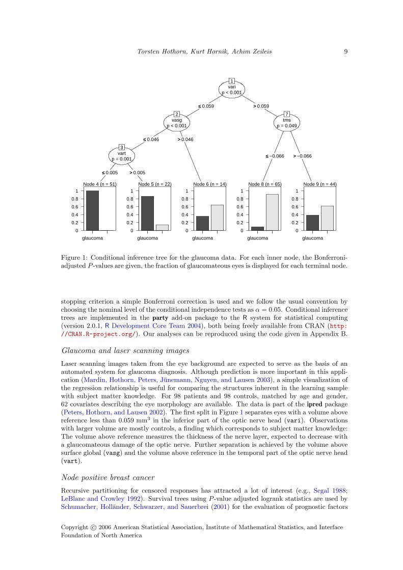
Figure 1: Conditional inference tree for the glaucoma data. For each inner node, the Bonferroni-adjusted P -values are given, the fraction of glaucomateous eyes is displayed for each terminal node.

stopping criterion a simple Bonferroni correction is used and we follow the usual convention bychoosing the nominal level of the conditional independence tests as α = 0.05. Conditional inferencetrees are implemented in the party add-on package to the R system for statistical computing(version 2.0.1, R Development Core Team 2004), both being freely available from CRAN (http://CRAN.R-project.org/). Our analyses can be reproduced using the code given in Appendix B.

Glaucoma and laser scanning images

Laser scanning images taken from the eye background are expected to serve as the basis of anautomated system for glaucoma diagnosis. Although prediction is more important in this appli-cation (Mardin, Hothorn, Peters, Junemann, Nguyen, and Lausen 2003), a simple visualization ofthe regression relationship is useful for comparing the structures inherent in the learning samplewith subject matter knowledge. For 98 patients and 98 controls, matched by age and gender,62 covariates describing the eye morphology are available. The data is part of the ipred package(Peters, Hothorn, and Lausen 2002). The first split in Figure 1 separates eyes with a volume abovereference less than 0.059 mm3 in the inferior part of the optic nerve head (vari). Observationswith larger volume are mostly controls, a finding which corresponds to subject matter knowledge:The volume above reference measures the thickness of the nerve layer, expected to decrease witha glaucomateous damage of the optic nerve. Further separation is achieved by the volume abovesurface global (vasg) and the volume above reference in the temporal part of the optic nerve head(vart).

Node positive breast cancer

Recursive partitioning for censored responses has attracted a lot of interest (e.g., Segal 1988;LeBlanc and Crowley 1992). Survival trees using P -value adjusted logrank statistics are used bySchumacher, Hollander, Schwarzer, and Sauerbrei (2001) for the evaluation of prognostic factors



http://CRAN.R-project.org/

http://CRAN.R-project.org/


pnodesp < 0.001

1

≤≤ 3 >> 3

horThp = 0.035

2

no yes

Node 3 (n = 248)

0 1 2 3 4 5 6 7

0

0.2

0.4

0.6

0.8

1Node 4 (n = 128)

0 1 2 3 4 5 6 7

0

0.2

0.4

0.6

0.8

1

progrecp < 0.001

5

≤≤ 20 >> 20

Node 6 (n = 144)

0 1 2 3 4 5 6 7

0

0.2

0.4

0.6

0.8

1Node 7 (n = 166)

0 1 2 3 4 5 6 7

0

0.2

0.4

0.6

0.8

1

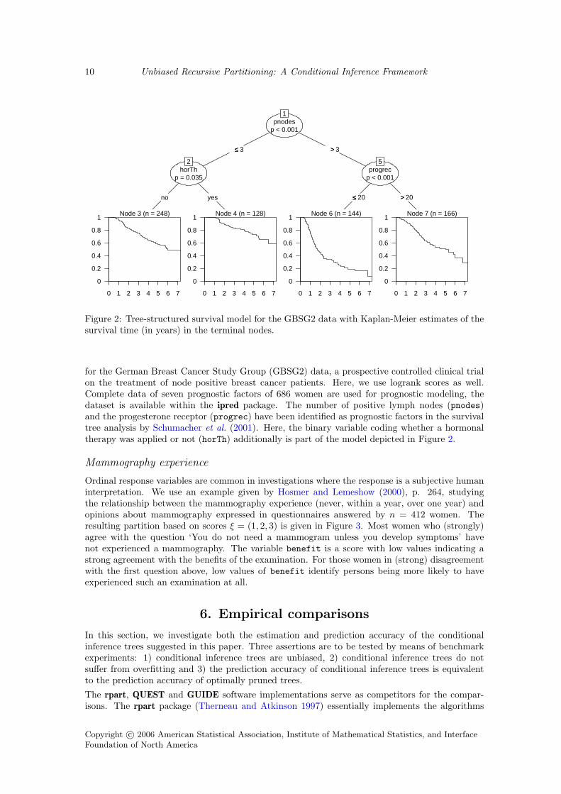
Figure 2: Tree-structured survival model for the GBSG2 data with Kaplan-Meier estimates of thesurvival time (in years) in the terminal nodes.

for the German Breast Cancer Study Group (GBSG2) data, a prospective controlled clinical trialon the treatment of node positive breast cancer patients. Here, we use logrank scores as well.Complete data of seven prognostic factors of 686 women are used for prognostic modeling, thedataset is available within the ipred package. The number of positive lymph nodes (pnodes)and the progesterone receptor (progrec) have been identified as prognostic factors in the survivaltree analysis by Schumacher et al. (2001). Here, the binary variable coding whether a hormonaltherapy was applied or not (horTh) additionally is part of the model depicted in Figure 2.

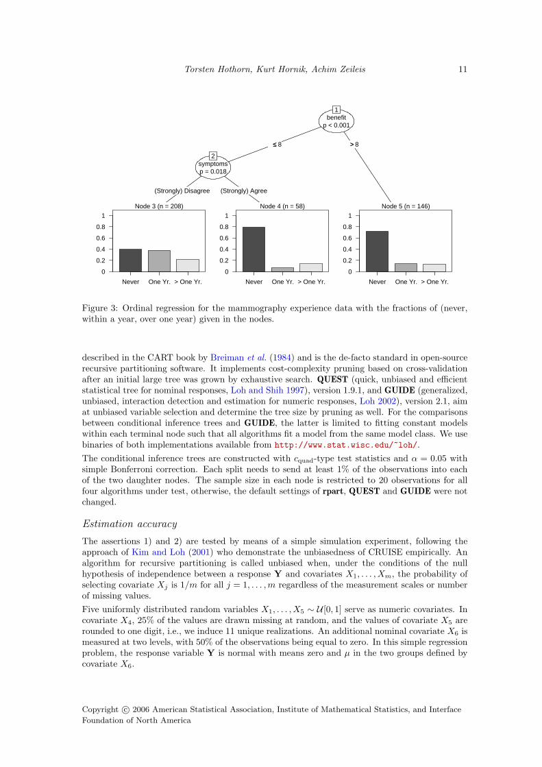
Mammography experience

Ordinal response variables are common in investigations where the response is a subjective humaninterpretation. We use an example given by Hosmer and Lemeshow (2000), p. 264, studyingthe relationship between the mammography experience (never, within a year, over one year) andopinions about mammography expressed in questionnaires answered by n = 412 women. Theresulting partition based on scores ξ = (1, 2, 3) is given in Figure 3. Most women who (strongly)agree with the question ‘You do not need a mammogram unless you develop symptoms’ havenot experienced a mammography. The variable benefit is a score with low values indicating astrong agreement with the benefits of the examination. For those women in (strong) disagreementwith the first question above, low values of benefit identify persons being more likely to haveexperienced such an examination at all.

6. Empirical comparisons

In this section, we investigate both the estimation and prediction accuracy of the conditionalinference trees suggested in this paper. Three assertions are to be tested by means of benchmarkexperiments: 1) conditional inference trees are unbiased, 2) conditional inference trees do notsuffer from overfitting and 3) the prediction accuracy of conditional inference trees is equivalentto the prediction accuracy of optimally pruned trees.

The rpart, QUEST and GUIDE software implementations serve as competitors for the compar-isons. The rpart package (Therneau and Atkinson 1997) essentially implements the algorithms



benefitp < 0.001

1

≤≤ 8 >> 8

symptomsp = 0.018

2

(Strongly) Disagree (Strongly) Agree

Node 3 (n = 208)

Never One Yr. > One Yr.

0

0.2

0.4

0.6

0.8

1

Node 4 (n = 58)


0

0.2

0.4

0.6

0.8

1

Node 5 (n = 146)


0

0.2

0.4

0.6

0.8

1

Figure 3: Ordinal regression for the mammography experience data with the fractions of (never,within a year, over one year) given in the nodes.

described in the CART book by Breiman et al. (1984) and is the de-facto standard in open-sourcerecursive partitioning software. It implements cost-complexity pruning based on cross-validationafter an initial large tree was grown by exhaustive search. QUEST (quick, unbiased and efficientstatistical tree for nominal responses, Loh and Shih 1997), version 1.9.1, and GUIDE (generalized,unbiased, interaction detection and estimation for numeric responses, Loh 2002), version 2.1, aimat unbiased variable selection and determine the tree size by pruning as well. For the comparisonsbetween conditional inference trees and GUIDE, the latter is limited to fitting constant modelswithin each terminal node such that all algorithms fit a model from the same model class. We usebinaries of both implementations available from http://www.stat.wisc.edu/~loh/.The conditional inference trees are constructed with cquad-type test statistics and α = 0.05 withsimple Bonferroni correction. Each split needs to send at least 1% of the observations into eachof the two daughter nodes. The sample size in each node is restricted to 20 observations for allfour algorithms under test, otherwise, the default settings of rpart, QUEST and GUIDE were notchanged.

Estimation accuracy

The assertions 1) and 2) are tested by means of a simple simulation experiment, following theapproach of Kim and Loh (2001) who demonstrate the unbiasedness of CRUISE empirically. Analgorithm for recursive partitioning is called unbiased when, under the conditions of the nullhypothesis of independence between a response Y and covariates X1, . . . , Xm, the probability ofselecting covariate Xj is 1/m for all j = 1, . . . ,m regardless of the measurement scales or numberof missing values.Five uniformly distributed random variables X1, . . . , X5 ∼ U [0, 1] serve as numeric covariates. Incovariate X4, 25% of the values are drawn missing at random, and the values of covariate X5 arerounded to one digit, i.e., we induce 11 unique realizations. An additional nominal covariate X6 ismeasured at two levels, with 50% of the observations being equal to zero. In this simple regressionproblem, the response variable Y is normal with means zero and µ in the two groups defined bycovariate X6.



http://www.stat.wisc.edu/~loh/


rpart Conditional Inference TreesEstimate 95% Confidence Interval Estimate 95% Confidence Interval

X1 ∼ U [0, 1] 0.231 (0.220, 0.243) 0.168 (0.159, 0.178)X2 ∼ U [0, 1] 0.225 (0.214, 0.236) 0.167 (0.157, 0.177)X3 ∼ U [0, 1] 0.227 (0.216, 0.238) 0.162 (0.153, 0.172)X4, missings 0.197 (0.187, 0.208) 0.169 (0.159, 0.179)X5, ties 0.100 (0.092, 0.108) 0.166 (0.156, 0.176)X6, binary 0.020 (0.017, 0.024) 0.169 (0.159, 0.179)

Table 1: Simulated probabilities of variable selection of six mutually independent variables whenthe response is independent of X1, . . . , X6, i.e., µ = 0. The results are based on 10,000 replications.

0.0 0.2 0.4 0.6 0.8 1.0

0.0

0.2

0.4

0.6

0.8

1.0

µ

Sim

ulat

ed P

ower

rpartcond. inf. trees

0.0 0.2 0.4 0.6 0.8 1.0

0.0

0.2

0.4

0.6

0.8

1.0

µ

Con

ditio

nal P

roba

bilit

y of

Cor

rect

Spl

it

Figure 4: Simulated power, i.e. the probability of a root split (left), and the simulated conditionalprobability of a correct split in variable X6 given that any root split was established (right) aredisplayed. The dotted horizontal line represents α = 0.05. The results are based on 10,000replications.

Y ∼{N (0, 1) if X6 = 0N (µ, 1) if X6 = 1.

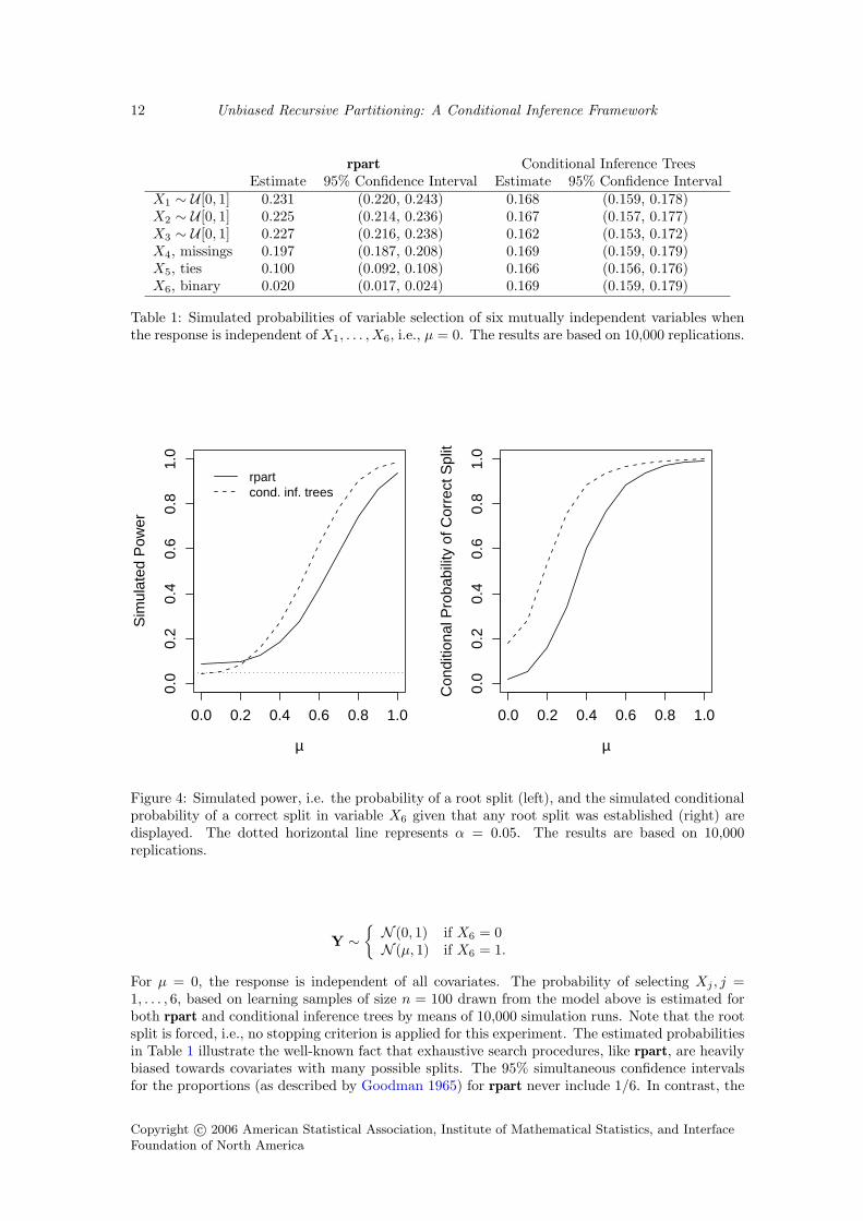
For µ = 0, the response is independent of all covariates. The probability of selecting Xj , j =1, . . . , 6, based on learning samples of size n = 100 drawn from the model above is estimated forboth rpart and conditional inference trees by means of 10,000 simulation runs. Note that the rootsplit is forced, i.e., no stopping criterion is applied for this experiment. The estimated probabilitiesin Table 1 illustrate the well-known fact that exhaustive search procedures, like rpart, are heavilybiased towards covariates with many possible splits. The 95% simultaneous confidence intervalsfor the proportions (as described by Goodman 1965) for rpart never include 1/6. In contrast, the



confidence intervals for the conditional inference trees always include the probability 1/6 expectedfor an unbiased variable selection, regardless of the measurement scale of the covariates. This resultindicates that the selection of covariates by asymptotic P -values of conditional independence testsis unbiased.From a practical point of view, two issues with greater relevance arise. On the one hand, theprobability of selecting any of the covariates for splitting for some µ ≥ 0 (power) and, on theother hand, the conditional probability of selecting the “correct split” in covariate X6 given anycovariate was selected for splitting are interesting criteria with respect to which the two algorithmsare compared. Figure 4 depicts the estimated probabilities for varying µ. For µ = 0, the probabilityof splitting the root node is 0.0435 for conditional inference trees and 0.0893 for rpart. Thus, theprobability of such an incorrect decision is bounded by α for the conditional inference trees and istwice as large for pruning as implemented in rpart. Under the alternative µ > 0, the conditionalinference trees are more powerful compared to rpart for µ > 0.2. For small values of µ the largerpower of rpart is due to the size distortion under the null hypothesis. In addition, the probability ofselecting X6 given that any covariate was selected is uniformly greater for the conditional inferencetrees.The advantageous properties of the conditional inference trees are obvious for the simple simulationmodel with one split only. We now extend our investigations to a simple regression tree with fourterminal nodes. The response variable is normal with mean µ depending on the covariates asfollows:

Y ∼

N (1, 1) if X6 = 0 and X1 < 0.5N (2, 1) if X6 = 0 and X1 ≥ 0.5N (3, 1) if X6 = 1 and X2 < 0.5N (4, 1) if X6 = 1 and X2 ≥ 0.5.

(4)

We will focus on two closely related criteria describing the partitions induced by the algorithms:the complexity of the induced partitions and the structure of the trees. The number of terminalnodes of a tree is a measure of the complexity of the model and can easily be compared with thenumber of cells in the true data partition defined by (4). However, the appropriate complexityof a tree does not ensure that the tree structure describes the true data partition well. Here, wemeasure the discrepancy between the true data partition and the partitions obtained from recursivepartitioning by the normalized mutual information (‘NMI’, Strehl and Ghosh 2003), essentiallythe mutual information of two partitions standardized by the entropy of both partitions. Valuesnear one indicate similar to equal partitions while values near zero are obtained for structurallydifferent partitions.For 1,000 learning samples of size n = 100 drawn from the simple tree model, Table 2 givesthe cross-tabulated number of terminal nodes of conditional inference trees and pruned exhaustivesearch trees computed by rpart. The null hypothesis of marginal homogeneity for ordered variables

Conditional Inference Trees2 3 4 5 6 ≥ 7

2 3 4 5 0 0 0 123 0 48 47 3 0 0 98

rpart 4 0 36 549 49 3 0 6375 0 12 134 25 1 0 1726 2 6 42 10 1 0 61

≥ 7 0 3 10 6 1 0 205 109 787 93 6 0 1000

Table 2: Number of terminal nodes for rpart and conditional inference trees when the learningsample is actually partitioned into four cells.




−0.3 −0.2 −0.1 0.0 0.1 0.2

02

46

8

NMI (rpart, true) − NMI (conditional inference tree, true)

Den

sity

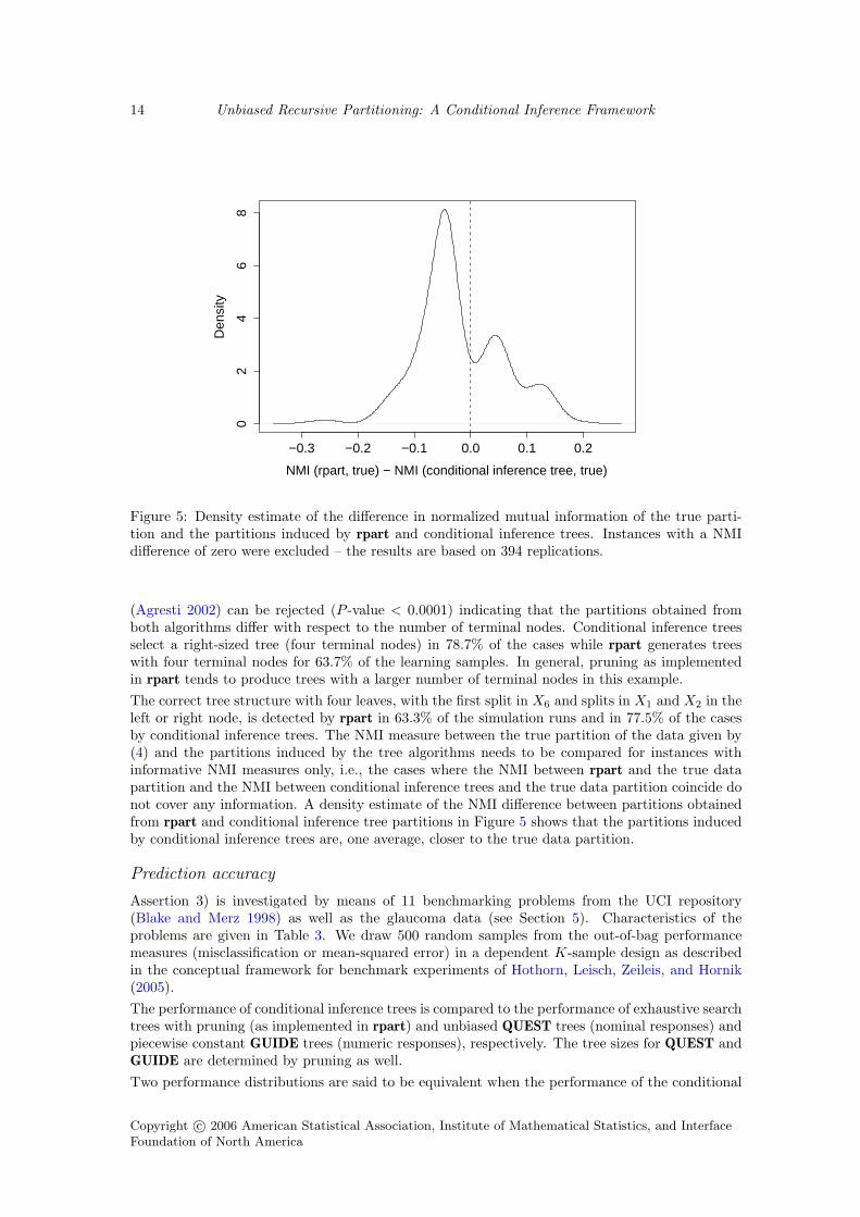
Figure 5: Density estimate of the difference in normalized mutual information of the true parti-tion and the partitions induced by rpart and conditional inference trees. Instances with a NMIdifference of zero were excluded – the results are based on 394 replications.

(Agresti 2002) can be rejected (P -value < 0.0001) indicating that the partitions obtained fromboth algorithms differ with respect to the number of terminal nodes. Conditional inference treesselect a right-sized tree (four terminal nodes) in 78.7% of the cases while rpart generates treeswith four terminal nodes for 63.7% of the learning samples. In general, pruning as implementedin rpart tends to produce trees with a larger number of terminal nodes in this example.The correct tree structure with four leaves, with the first split in X6 and splits in X1 and X2 in theleft or right node, is detected by rpart in 63.3% of the simulation runs and in 77.5% of the casesby conditional inference trees. The NMI measure between the true partition of the data given by(4) and the partitions induced by the tree algorithms needs to be compared for instances withinformative NMI measures only, i.e., the cases where the NMI between rpart and the true datapartition and the NMI between conditional inference trees and the true data partition coincide donot cover any information. A density estimate of the NMI difference between partitions obtainedfrom rpart and conditional inference tree partitions in Figure 5 shows that the partitions inducedby conditional inference trees are, one average, closer to the true data partition.

Prediction accuracy

Assertion 3) is investigated by means of 11 benchmarking problems from the UCI repository(Blake and Merz 1998) as well as the glaucoma data (see Section 5). Characteristics of theproblems are given in Table 3. We draw 500 random samples from the out-of-bag performancemeasures (misclassification or mean-squared error) in a dependent K-sample design as describedin the conceptual framework for benchmark experiments of Hothorn, Leisch, Zeileis, and Hornik(2005).The performance of conditional inference trees is compared to the performance of exhaustive searchtrees with pruning (as implemented in rpart) and unbiased QUEST trees (nominal responses) andpiecewise constant GUIDE trees (numeric responses), respectively. The tree sizes for QUEST andGUIDE are determined by pruning as well.Two performance distributions are said to be equivalent when the performance of the conditional



J n NA m nominal ordinal continuousBoston Housing – 506 – 13 – – 13Ozone – 361 158 12 3 – 9Servo – 167 – 4 4 – –Breast Cancer 2 699 16 9 4 5 –Diabetes 2 768 – 8 – – 8Glass 6 214 – 9 – – 9Glaucoma 2 196 – 62 – – 62Ionosphere 2 351 – 33 1 – 32Sonar 2 208 – 60 – – 60Soybean 19 683 121 35 35 5 –Vehicle 4 846 – 19 – – 19Vowel 11 990 – 10 1 – 9

Table 3: Summary of the benchmarking problems showing the number of classes of a nominalresponse J (‘–’ indicates a continuous response), the number of observations n, the number ofobservations with at least one missing value (NA) as well as the measurement scale and numberm of the covariates.

inference trees compared to the performance of one competitor (rpart, QUEST or GUIDE) doesnot differ by an amount of more than 10%. The null hypothesis of non-equivalent performancesis then defined in terms of the ratio of the expectations of the performance distribution of condi-tional inference trees and its competitors. Equivalence can be established at level α based on twoone-sided level α tests by the intersection-union principle (Berger and Hsu 1996). Here, this corre-sponds to a rejection of the null hypothesis of non-equivalence performances at the 5% level whenthe 90% two-sided Fieller (1940) confidence interval for the ratio of the performance expectationsis completely included in the equivalence range (0.9, 1.1).

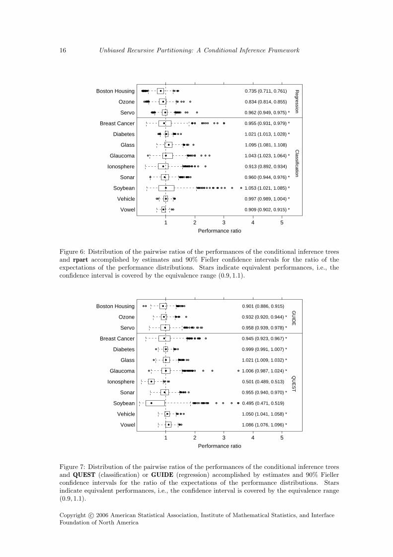
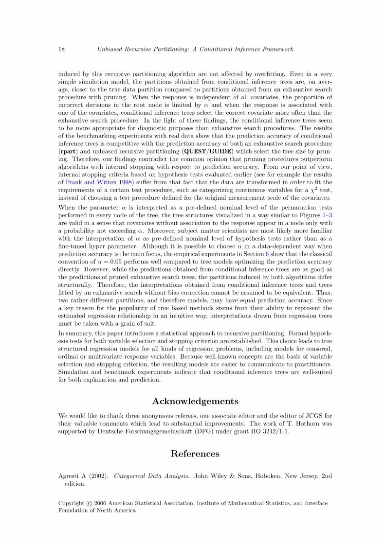
The boxplots of the pairwise ratios of the performance measure evaluated for conditional in-ference trees and pruned exhaustive search trees (rpart, Figure 6) and pruned unbiased trees(QUEST/GUIDE, Figure 7) are accomplished by estimates of the ratio of the expected perfor-mances and corresponding Fieller confidence intervals. For example, an estimate of the ratio ofthe misclassification errors of rpart and conditional inference trees for the glaucoma data of 1.043means that the misclassification error of conditional inference trees is 4.3% larger than the mis-classification error of rpart. The confidence interval of (1.023, 1.064) leads to the conclusion thatthis inferiority is within the pre-defined equivalence margin of ±10% and thus the performance ofconditional inference trees is on par with the performance of rpart for the glaucoma data.

Equivalent performance between conditional inference trees and rpart cannot be postulated for theGlass data. The performance of the conditional inference trees is roughly 10% worse comparedwith rpart. In all other cases, the performance of conditional inference trees is better than orequivalent to the performance of exhaustive search (rpart) and unbiased procedures (QUEST orGUIDE) with pruning. The conditional inference trees perform better compared to rpart treesby a magnitude of 25% (Boston Housing), 10% (Ionosphere) and 15% (Ozone). The improvementupon unbiased QUEST and piecewise constant GUIDE models is 10% for the Boston Housingdata and 50% for the Ionosphere and Soybean data. For all other problems, the performance ofconditional inference trees fitted within a permutation testing framework can be assumed to beequivalent to the performance of all three competitors.

The simulation experiments with model (4) presented in the first paragraph on estimation accuracylead to the impression that the partitions induced by rpart trees are structurally different from thepartition induced by conditional inference trees. Because the ‘true’ partition is unknown for thedatasets used here, we compare the partitions obtained from conditional inference trees and rpartby their normalized mutual information. The median normalized mutual information is 0.447 anda bivariate density estimate depicted in Figure 8 does not indicate any relationship between the




Performance ratio

1 2 3 4 5

Vowel

Vehicle

Soybean

Sonar

Ionosphere

Glaucoma

Glass

Diabetes

Breast Cancer

Servo

Ozone

Boston Housing ●●● ●●● ● ●●● ●● ●● ●●● ● ●●● ●●●●●● ●●●

● ●● ● ●● ●● ●●● ● ●●●● ●

●●●● ●● ●●● ●●●●●●● ●●

● ●● ●● ●●●●● ●

● ●●● ● ●●● ● ●●●● ●● ●●

● ● ●● ●●● ●●●● ●●●● ● ●●● ●●●

●●●●● ●●●● ●●●●● ● ●● ●●●●● ●

● ●● ● ● ●●● ● ●● ●● ●●● ●●●● ●● ● ●● ●

● ●●● ●●● ●●● ●● ●● ● ●● ●

● ● ●● ●●●● ● ● ●● ●● ●● ●●●●

● ●●●●●●

● ●●

0.735 (0.711, 0.761)

0.834 (0.814, 0.855)

0.962 (0.949, 0.975) *

0.955 (0.931, 0.979) *

1.021 (1.013, 1.028) *

1.095 (1.081, 1.108)

1.043 (1.023, 1.064) *

0.913 (0.892, 0.934)

0.960 (0.944, 0.976) *

1.053 (1.021, 1.085) *

0.997 (0.989, 1.004) *

0.909 (0.902, 0.915) *

Regression

Classification

Figure 6: Distribution of the pairwise ratios of the performances of the conditional inference treesand rpart accomplished by estimates and 90% Fieller confidence intervals for the ratio of theexpectations of the performance distributions. Stars indicate equivalent performances, i.e., theconfidence interval is covered by the equivalence range (0.9, 1.1).

Performance ratio

1 2 3 4 5

Vowel

Vehicle

Soybean

Sonar

Ionosphere

Glaucoma

Glass

Diabetes

Breast Cancer

Servo

Ozone

Boston Housing ● ●●● ●● ●●●● ●● ●●● ●

● ● ●●●●●● ●●● ●● ●●● ●●● ●●●

● ●●● ●●● ●●● ●● ●● ● ●

● ●● ●● ●

● ●● ●●●●●● ●●● ●

● ● ● ●● ●●

● ●●● ●● ●●

● ● ●●●● ●●● ● ●●●● ●● ●● ●● ●● ●●● ●

● ● ●● ●● ●● ●

● ●● ●●●● ●● ●● ●● ●● ●● ●●

● ● ●●●● ●●● ● ●●● ●●●● ●● ●●● ● ●

● ●● ●●

0.901 (0.886, 0.915)

0.932 (0.920, 0.944) *

0.958 (0.939, 0.978) *

0.945 (0.923, 0.967) *

0.999 (0.991, 1.007) *

1.021 (1.009, 1.032) *

1.006 (0.987, 1.024) *

0.501 (0.489, 0.513)

0.955 (0.940, 0.970) *

0.495 (0.471, 0.519)

1.050 (1.041, 1.058) *

1.086 (1.076, 1.096) *

GU

IDE

QU

ES

T

Figure 7: Distribution of the pairwise ratios of the performances of the conditional inference treesand QUEST (classification) or GUIDE (regression) accomplished by estimates and 90% Fiellerconfidence intervals for the ratio of the expectations of the performance distributions. Starsindicate equivalent performances, i.e., the confidence interval is covered by the equivalence range(0.9, 1.1).



0.0 0.5 1.0 1.5 2.0

0.0

0.2

0.4

0.6

0.8

1.0

Performance ratio

NM

I

dx$x

Figure 8: Distribution of the pairwise performance ratios of conditional inference trees and rpartand the normalized mutual information measuring the discrepancy of the induced partitions.

ratio of the performances and the discrepancy of the partitions.

This results is interesting from a practical point of view. It implies that two recursive partitioningalgorithms can achieve the same prediction accuracy but, at the same time, represent structurallydifferent regression relationships, i.e., different models and thus may lead to different conclusionsabout the influence of certain covariates on the response.

7. Discussion

In this paper, recursive binary partitioning with piecewise constant fits, a popular tool for regres-sion analysis, is embedded into a well-defined framework of conditional inference procedures. Boththe overfitting and variable selection problems induced by a recursive fitting procedure are solvedby the application of the appropriate statistical test procedures to both variable selection and stop-ping. Therefore, the conditional inference trees suggested in this paper are not just heuristics butnon-parametric models with well-defined theoretical background. The methodology is generallyapplicable to regression problems with arbitrary measurement scales of responses and covariates.In addition to its advantageous statistical properties, our framework is computationally attractivesince we do not need to evaluate all 2K−1 − 1 possible splits of a nominal covariate at K levelsfor the variable selection. In contrast to algorithms incorporating pruning based on resampling,the models suggested here can be fitted deterministically, provided that the exact conditionaldistribution is not approximated by Monte-Carlo methods.

The simulation and benchmarking experiments in Section 6 support two conclusions: Conditionalinference trees as suggested in this paper select variables in an unbiased way and the partitions




induced by this recursive partitioning algorithm are not affected by overfitting. Even in a verysimple simulation model, the partitions obtained from conditional inference trees are, on aver-age, closer to the true data partition compared to partitions obtained from an exhaustive searchprocedure with pruning. When the response is independent of all covariates, the proportion ofincorrect decisions in the root node is limited by α and when the response is associated withone of the covariates, conditional inference trees select the correct covariate more often than theexhaustive search procedure. In the light of these findings, the conditional inference trees seemto be more appropriate for diagnostic purposes than exhaustive search procedures. The resultsof the benchmarking experiments with real data show that the prediction accuracy of conditionalinference trees is competitive with the prediction accuracy of both an exhaustive search procedure(rpart) and unbiased recursive partitioning (QUEST/GUIDE) which select the tree size by prun-ing. Therefore, our findings contradict the common opinion that pruning procedures outperformalgorithms with internal stopping with respect to prediction accuracy. From our point of view,internal stopping criteria based on hypothesis tests evaluated earlier (see for example the resultsof Frank and Witten 1998) suffer from that fact that the data are transformed in order to fit therequirements of a certain test procedure, such as categorizing continuous variables for a χ2 test,instead of choosing a test procedure defined for the original measurement scale of the covariates.

When the parameter α is interpreted as a pre-defined nominal level of the permutation testsperformed in every node of the tree, the tree structures visualized in a way similar to Figures 1–3are valid in a sense that covariates without association to the response appear in a node only witha probability not exceeding α. Moreover, subject matter scientists are most likely more familiarwith the interpretation of α as pre-defined nominal level of hypothesis tests rather than as afine-tuned hyper parameter. Although it is possible to choose α in a data-dependent way whenprediction accuracy is the main focus, the empirical experiments in Section 6 show that the classicalconvention of α = 0.05 performs well compared to tree models optimizing the prediction accuracydirectly. However, while the predictions obtained from conditional inference trees are as good asthe predictions of pruned exhaustive search trees, the partitions induced by both algorithms differstructurally. Therefore, the interpretations obtained from conditional inference trees and treesfitted by an exhaustive search without bias correction cannot be assumed to be equivalent. Thus,two rather different partitions, and therefore models, may have equal prediction accuracy. Sincea key reason for the popularity of tree based methods stems from their ability to represent theestimated regression relationship in an intuitive way, interpretations drawn from regression treesmust be taken with a grain of salt.

In summary, this paper introduces a statistical approach to recursive partitioning. Formal hypoth-esis tests for both variable selection and stopping criterion are established. This choice leads to treestructured regression models for all kinds of regression problems, including models for censored,ordinal or multivariate response variables. Because well-known concepts are the basis of variableselection and stopping criterion, the resulting models are easier to communicate to practitioners.Simulation and benchmark experiments indicate that conditional inference trees are well-suitedfor both explanation and prediction.

Acknowledgements

We would like to thank three anonymous referees, one associate editor and the editor of JCGS fortheir valuable comments which lead to substantial improvements. The work of T. Hothorn wassupported by Deutsche Forschungsgemeinschaft (DFG) under grant HO 3242/1-1.

References

Agresti A (2002). Categorical Data Analysis. John Wiley & Sons, Hoboken, New Jersey, 2ndedition.



Berger RL, Hsu JC (1996). “Bioequivalence Trials, Intersection-Union Tests and EquivalenceConfidence Sets.” Statistical Science, 11(4), 283–319. With discussion.

Blake C, Merz C (1998). “UCI Repository of Machine Learning Databases.” URL http://www.ics.uci.edu/~mlearn/MLRepository.html.

Breiman L, Friedman JH, Olshen RA, Stone CJ (1984). Classification and Regression Trees.Wadsworth, California.

De’ath G (2002). “Multivariate Regression Trees: A New Technique For Modeling Species-Environment Relationships.” Ecology, 83(4), 1105–1117.

Dobra A, Gehrke J (2001). “Bias Correction in Classification Tree Construction.” In “Proceedingsof the Eighteenth International Conference on Machine Learning,”pp. 90–97. Morgan KaufmannPublishers Inc. ISBN 1-55860-778-1.

Fieller EC (1940). “The Biological Standardization of Insulin.” Journal of the Royal StatisticalSociety, Supplement, 7, 1–64.

Frank E, Witten IH (1998). “Using a Permutation Test for Attribute Selection in Decision Trees.”In “Proceedings of the Fifteenth International Conference on Machine Learning,” pp. 152–160.Morgan Kaufmann Publishers Inc. ISBN 1-55860-556-8.

Genz A (1992). “Numerical Computation of Multivariate Normal Probabilities.” Journal of Com-putational and Graphical Statistics, 1, 141–149.

Goodman LA (1965). “On Simultaneous Confidence Intervals for Multinomial Proportions.” Tech-nometrics, 7(2), 247–254.

Hosmer DW, Lemeshow S (2000). Applied Logistic Regression. John Wiley & Sons, New York,2nd edition.

Hothorn T, Hornik K, van de Wiel MA, Zeileis A (2006). “A Lego System for Conditional Infer-ence.” The American Statistician, 60, 257–263. doi:10.1198/000313006X118430.

Hothorn T, Leisch F, Zeileis A, Hornik K (2005). “The Design and Analysis of Benchmark Exper-iments.” Journal of Computational and Graphical Statistics, 14(3), 675–699.

Jensen DD, Cohen PR (2000). “Multiple Comparisons in Induction Algorithms.” Machine Learn-ing, 38, 309–338.

Kass G (1980). “An Exploratory Technique for Investigating Large Quantities of Categorical Data.”Applied Statistics, 29(2), 119–127.

Kim H, Loh WY (2001). “Classification Trees With Unbiased Multiway Splits.” Journal of theAmerican Statistical Association, 96(454), 589–604.

Kim H, Loh WY (2003). “Classification Trees with Bivariate Linear Discriminant Node Models.”Journal of Computational and Graphical Statistics, 12, 512–530.

Lausen B, Hothorn T, Bretz F, Schumacher M (2004). “Assessment of Optimal Selected PrognosticFactors.” Biometrical Journal, 46(3), 364–374.

Lausen B, Schumacher M (1992). “Maximally Selected Rank Statistics.” Biometrics, 48, 73–85.

LeBlanc M, Crowley J (1992). “Relative Risk Trees for Censored Survival Data.” Biometrics, 48,411–425.

LeBlanc M, Crowley J (1993). “Survival Trees by Goodness of Split.” Journal of the AmericanStatistical Association, 88(422), 457–467.



http://www.ics.uci.edu/~mlearn/MLRepository.html

http://www.ics.uci.edu/~mlearn/MLRepository.html

http://dx.doi.org/10.1198/000313006X118430


Loh WY (2002). “Regression Trees With Unbiased Variable Selection And Interaction Detection.”Statistica Sinica, 12, 361–386.

Loh WY, Shih YS (1997). “Split Selection Methods for Classification Trees.” Statistica Sinica, 7,815–840.

Loh WY, Vanichsetakul N (1988). “Tree-Structured Classification via Generalized DiscriminantAnalysis.” Journal of the American Statistical Association, 83, 715–725. With discussion.

Mardin CY, Hothorn T, Peters A, Junemann AG, Nguyen NX, Lausen B (2003). “New GlaucomaClassification Method Based on Standard HRT Parameters by Bagging Classification Trees.”Journal of Glaucoma, 12(4), 340–346.

Martin JK (1997). “An Exact Probability Metric for Decision Tree Splitting and Stopping.”Machine Learning, 28, 257–291.

Miller R, Siegmund D (1982). “Maximally Selected Chi Square Statistics.” Biometrics, 38, 1011–1016.

Mingers J (1987). “Expert Systems – Rule Induction with Statistical Data.” Journal of theOperations Research Society, 38(1), 39–47.

Molinaro AM, Dudoit S, van der Laan MJ (2004). “Tree-based Multivariate Regression and DensityEstimation with Right-Censored Data.” Journal of Multivariate Analysis, 90(1), 154–177.

Morgan JN, Sonquist JA (1963). “Problems in the Analysis of Survey Data, and a Proposal.”Journal of the American Statistical Association, 58, 415–434.

Murthy SK (1998). “Automatic Construction of Decision Trees from Data: A Multi-DisciplinarySurvey.” Data Mining and Knowledge Discovery, 2, 345–389.

Noh HG, Song MS, Park SH (2004). “An Unbiased Method for Constructing Multilabel Classifi-cation Trees.” Computational Statistics & Data Analysis, 47(1), 149–164.

O’Brien SM (2004). “Cutpoint Selection for Categorizing a Continuous Predictor.” Biometrics,60, 504–509.

Peters A, Hothorn T, Lausen B (2002). “ipred: Improved Predictors.” R News, 2(2), 33–36. ISSN1609-3631, URL http://CRAN.R-project.org/doc/Rnews/.

Quinlan JR (1993). C4.5: Programs for Machine Learning. Morgan Kaufmann Publishers Inc.,San Mateo, California.

Rasch D (1995). Mathematische Statistik. Johann Ambrosius Barth Verlag, Heidelberg, Leipzig.

R Development Core Team (2004). R: A Language and Environment for Statistical Computing.R Foundation for Statistical Computing, Vienna, Austria. ISBN 3-900051-00-3, URL http://www.R-project.org/.

Schumacher M, Hollander N, Schwarzer G, Sauerbrei W (2001). “Prognostic Factor Studies.” InJ Crowley (ed.), “Statistics in Clinical Oncology,” pp. 321–378. Marcel Dekker, New York, Basel.

Segal MR (1988). “Regression Trees for Censored Data.” Biometrics, 44, 35–47.

Shih YS (1999). “Families of Splitting Criteria for Classification Trees.” Statistics and Computing,9, 309–315.

Shih YS (2004). “A Note on Split Selection Bias in Classification Trees.” Computational Statistics& Data Analysis, 45, 457–466.


http://CRAN.R-project.org/doc/Rnews/

http://www.R-project.org/

http://www.R-project.org/


Strasser H, Weber C (1999). “On the Asymptotic Theory of Permutation Statistics.” MathematicalMethods of Statistics, 8, 220–250. URL http://epub.wu-wien.ac.at/dyn/openURL?id=oai:epub.wu-wien.ac.at:epub-wu-01_94c.

Strehl A, Ghosh J (2003). “Cluster Ensembles - A Knowledge Reuse Framework for CombiningMultiple Partitions.” Journal of Machine Learning Research, 3, 583–617.

Therneau TM, Atkinson EJ (1997). “An Introduction to Recursive Partitioning using the rpartRoutine.” Technical Report 61, Section of Biostatistics, Mayo Clinic, Rochester. URL http://www.mayo.edu/hsr/techrpt/61.pdf.

Westfall PH, Young SS (1993). Resampling-based Multiple Testing. John Wiley & Sons, New York.

White AP, Liu WZ (1994). “Bias in Information-based Measures in Decision Tree Induction.”Machine Learning, 15, 321–329.

Zhang H (1998). “Classification Trees for Multiple Binary Responses.” Journal of the AmericanStatistical Association, 93, 180–193.

Appendix A

An equivalent but computational simpler formulation of the linear statistic for case weights greaterthan one can be written as follows. Let a = (a1, . . . , aw·), al ∈ {1, . . . , n}, l = 1, . . . ,w·, denotethe vector of observation indices, with index i occuring wi times. Instead of recycling the ithobservation wi times it is sufficient to implement the index vector a into the computation of thetest statistic and its expectation and covariance. For one permutation σ of {1, . . . ,w·}, the linearstatistic (1) may be written as

Tj(Ln,w) = vec

(w·∑

k=1

gj(Xjak)h(Yσ(a)k

, (Y1, . . . ,Yn))>)∈ Rpjq

now taking case weights greater zero into account.

Appendix B

The results shown in Section 5 are, up to some labelling, reproducible using the following R code:

library("party")

data("GlaucomaM", package = "ipred")

plot(ctree(Class ~ ., data = GlaucomaM))

data("GBSG2", package = "ipred")

plot(ctree(Surv(time, cens) ~ ., data = GBSG2))

data("mammoexp", package = "party")

plot(ctree(ME ~ ., data = mammoexp))



http://epub.wu-wien.ac.at/dyn/openURL?id=oai:epub.wu-wien.ac.at:epub-wu-01_94c

http://epub.wu-wien.ac.at/dyn/openURL?id=oai:epub.wu-wien.ac.at:epub-wu-01_94c

http://www.mayo.edu/hsr/techrpt/61.pdf

http://www.mayo.edu/hsr/techrpt/61.pdf

unbiased recursive partitioning: a conditional inference...

Documents