uncertainty analysis and model “validation” or confidence building
TRANSCRIPT

Uncertainty Analysis
and
Model “Validation” or Confidence Building

Conclusions
• Calibrations are non-unique.
• A good calibration (even if ARM = 0) does not ensure that the model will make good predictions.
• Field data are essential in constraining the model so that the model can capture the essential features of the system.
• Modelers need to maintain a healthy skepticism about their results.

• Head predictions are more robust (consistent among different calibrated models) than transport (particle tracking) predictions.
Conclusions
• Need for an uncertainty analysis to accompany calibration results and predictions.
Ideally models should be maintained for the long termand updated to establish confidence in the model.Rather than a single calibration exercise, a continualprocess of confidence building is needed.
Uncertainty in the Calibration
Involves uncertainty in:
Parameter values
Conceptual model including boundary conditions,zonation, geometry, etc.
Targets

Zonation
Kriging

To use conventional inverse models/parameter estimationmodels in calibration, you need to have a pretty good idea of zonation (of K, for example).
Also need to identify reasonable ranges for thecalibration parameters and weights.
(New version of PEST with pilot points does not need zonation as it works with continuous distribution of parameter values.)
Zonation vs Pilot Points

• Field data are essential in constraining the model so that the model can capture the essential features of the system.
Parameter Values

Calibration Targets
calibration value
associated error
20.24 m
0.80 m
Target with relativelylarge associated error.
Target with smaller associated error.
Need to establish model specific calibration criteria and define targets including associated error.

Examples of Sources of Errorin a Calibration Target
• Surveying errors • Errors in measuring water levels• Interpolation error• Transient effects• Scaling effects• Unmodeled heterogeneities

Importance of Flux Targets
When recharge rate (R) is a calibration parameter, calibrating to fluxes can help in estimating K and/or R.
R was not a calibration parameter in our final project.

H1H2
q = KI
In this example, flux information helps calibrate K.

Here discharge information helps calibrate R.
Q

H1H2
q = KI
In this example, flux information helps calibrate K.

All water discharges to the playa.Calibration to ET merely fine tunesthe discharge rates within the playaarea. Calibration to ET does nothelp calibrate the heads and K valuesexcept in the immediate vicinityof the playa.
In our example, total recharge is known/assumed to be 7.14E08 ft3/year and discharge = recharge.

Smith Creek Valley (Thomas et al., 1989)
Calibration Objectives (matching targets)
1. Heads within 10 ft of measured heads. Allows forMeasurement error and interpolation error.
2. Absolute residual mean between measured and simulated heads close to zero (0.22 ft) and standard deviation minimal (4.5 ft).
3. Head difference between layers 1&2 within 2 ft of field values.
4. Distribution of ET and ET rates match field estimates.

0
0.5
1
1.5
2
2.5
3
3.5
4
4.5
0 0.5 1 1.5 2 2.5 3
Calibrated ARMP
red
icte
d A
RM
-ta
rge
ts
0
2
4
6
8
10
12
14
0 0.5 1 1.5 2 2.5 3
Calibrated ARM
Pre
dic
ted
AR
M-p
um
pin
g w
ells
Includes results from2006 and 4 other years
724 Project Results
A “good” calibrationdoes not guarantee
an accurate prediction.
?

Sensitivity analysis to analyze uncertaintyin the calibration
Use an inverse model (automated calibration) to quantify uncertainties and optimize the calibration.
Perform sensitivity analysis during calibration.
Sensitivity coefficients

(Zheng and Bennett)
Sensitivityanalysis performedduring the calibration
Steps in Modeling
calibrationloop

Uncertainty in the Prediction
Involves uncertainty in how parameter values(e.g., recharge) or pumping rates will varyin the future.
Reflects uncertainty in the calibration.

Stochastic simulation
Ways to quantify uncertaintyin the prediction
Scenario analysis - stresses
Sensitivity analysis - parameters

(Zheng and Bennett)
Sensitivityanalysis performedafter the prediction
Steps in Modeling
Traditional Paradigm

Multi-modelAnalysis (MMA) Predictions and sensitivity
analysis are insidethe calibration loop
From J. Doherty 2007
New Paradigmfor Sensitivity& ScenarioAnalysis

Stochastic simulation
Ways to quantify uncertaintyin the prediction
Scenario analysis - stresses
Sensitivity analysis - parameters

MADE site – Feehley and Zheng, 2000, WRR 36(9).
Stochastic simulation Stochastic modeling option available in GW Vistas

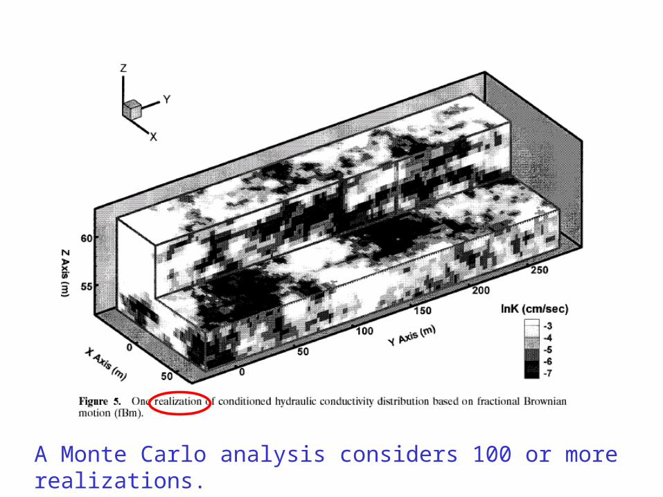
A Monte Carlo analysis considers 100 or more realizations.

0
20
40
60
80
100
120
140
1 2 3 4 5 6 7
Drawdown at pumping well
nu
mb
er o
f re
aliz
atio
ns

Zheng & BennettFig. 13.2

Hydraulic conductivity
Initial concentrations(plume configuration)
Both
Zheng & BennettFig. 13.5

Reducing Uncertainty
Hard data only
Soft and hard data
With inverse flow modeling
Hypotheticalexample
truth
Z&BFig. 13.6

How do we “validate” a model so thatwe have confidence that it will makeaccurate predictions?
Confidence Building

Modeling Chronology
1960’s Flow models are great!
1970’s Contaminant transport models are great!
1975 What about uncertainty of flow models?
1980s Contaminant transport models don’t work. (because of failure to account for heterogeneity)
1990s Are models reliable? Concerns overreliability in predictions arose over efforts to modelgeologic repositories for high level radioactive waste.

“The objective of model validation is to determine how well the mathematical representation of the processes describes the actual system behavior in terms of the degree of correlation between model calculations and actual measured data”(NRC, 1990)
Hmmmmm…. Sounds like calibration…What they really mean is that a valid model willyield an accurate prediction.

Oreskes et al. (1994): paper in Science
Calibration = forced empirical adequacy
Verification = assertion of truth (possible in a closed system, e.g., testing of codes)
Validation = establishment of legitimacy (does not contain obvious errors), confirmation, confidence building
What constitutes “validation”? (code vs. model)
NRC study (1990): Model validation is not possible.

How to build confidence in a model
Calibration (history matching) steady-state calibration(s) transient calibration
“Verification” requires an independent set of field data
Post-Audit: requires waiting for prediction to occur
Models as interactive management tools (e.g., theAEM model of The Netherlands)

HAPPY MODELING!