uncertainty analysis for the integration of seismic and...

Geophysical Prospecting, 2011, 59, 609–626 doi: 10.1111/j.1365-2478.2010.00937.x

Uncertainty analysis for the integration of seismic and controlledsource electro-magnetic data

Myoung Jae Kwon∗ and Roel SniederCenter for Wave Phenomena, Department of Geophysics, Colorado School of Mines, 1500 Illinois St., Golden, CO 80401, USA

Received September 2009, revision accepted October 2010

ABSTRACTWe study the appraisal problem for the joint inversion of seismic and controlledsource electro-magnetic (CSEM) data and utilize rock-physics models to integratethese two disparate data sets. The appraisal problem is solved by adopting a Bayesianmodel and we incorporate four representative sources of uncertainty. These are un-certainties in 1) seismic wave velocity, 2) electric conductivity, 3) seismic data and 4)CSEM data. The uncertainties in porosity and water saturation are quantified by aposterior random sampling in the model space of porosity and water saturation in amarine one-dimensional structure. We study the relative contributions from the fourindividual sources of uncertainty by performing several statistical experiments. Theuncertainties in the seismic wave velocity and electric conductivity play a more sig-nificant role on the variation of posterior uncertainty than do the seismic and CSEMdata noise. The numerical simulations also show that the uncertainty in porosity ismost affected by the uncertainty in the seismic wave velocity and that the uncertaintyin water saturation is most influenced by the uncertainty in electric conductivity.The framework of the uncertainty analysis presented in this study can be utilized toeffectively reduce the uncertainty of the porosity and water saturation derived fromthe integration of seismic and CSEM data.

Key words: Controlled source electro-magnetic, Metropolis-Hastings algorithm,Uncertainty analysis.

INTRODUCTION

The controlled source electro-magnetic (CSEM) method hasbeen studied for the last few decades (Chave and Cox 1982;Cox et al. 1986) and its application for the delineation of ahydrocarbon reservoir has recently been discussed (Constableand Srnka 2007). Currently, there is an increasing interest inthe integration of the seismic and CSEM methods in deep ma-rine exploration (Harris and MacGregor 2006). Although theCSEM method has less resolution than the seismic method, itprovides extra information about, for example, electric con-ductivity. This property is important for the economic evalua-tion of reservoirs. Therefore, the CSEM method is considered

∗E-mail: [email protected]

an effective complementary tool when combined with seismicexploration.

The seismic and CSEM methods are disparate explorationtechniques that are sensitive to different medium properties:the seismic method is sensitive to density and seismic wavevelocity and the CSEM method to electric conductivity. Therehave been several approaches for joint inversion that integratedisparate data sets. Some of them assume a common structure(Musil, Maurer and Green 2003) or similar structural vari-ations of different medium properties (Gallardo and Meju2004; Hu, Abubakar and Habashy 2009). More recently, theapplication of rock-physics models for joint inversion has beenstudied (Hoversten et al. 2006). Rock-physics models enableus to interrelate seismic wave velocity and electric conduc-tivity with the reservoir parameters such as porosity, wa-ter saturation, or permeability. The main advantage of the

C© 2011 European Association of Geoscientists & Engineers 609

610 M.J. Kwon and R. Snieder

approach is that these reservoir parameters have great eco-nomic importance. The application of a rock-physics model islimited, however, by the fact that such a model is site-specificand there are not yet any universal solutions to the inverseproblem. Furthermore, even for a particular area of interest,any rock-physics model is generally described as a cloud ofsamples. These limitations imply that joint inversion via arock-physics model intrinsically necessitates a stochastic ap-proach. Stochastic inversion has recently been studied for seis-mic inversion (Spikes et al. 2007) and joint inversion of seismicand CSEM data (Chen et al. 2007). The contributions of rock-physics model uncertainties are also being studied (Chen andDickens 2009). Generally, the accuracy of joint inversion ofseismic and CSEM data via rock-physics models is limited bythe uncertainty of the rock-physics model as well as by datanoise. The contribution of seismic and CSEM data noise onthe joint inversion via rock-physics models, however, has notyet been studied. Moreover, it is not yet understood whetherrock-physics model uncertainties play a more significant rolethan data noise on the joint inversion process.

We aim to investigate the relative contribution of differentsources of overall uncertainty that arise when we use rock-physics models for joint inversion. These include seismic datanoise, CSEM data noise and uncertainties of rock-physicsmodels. We implement several numerical experiments thatreflect scenarios we may encounter in practice and comparethe uncertainties in the inferred parameters. The comparisonreveals the relative contributions of different sources of un-certainty and we can utilize the procedure to more effectivelyreduce the uncertainty, depending on whether our interestsfocus on porosity or water saturation.

METHODOLOGY

The goal of geophysical inversion is to make quantitative in-ferences about the earth from noisy data. There are mainlytwo different approaches for attaining this goal: in one, theunknown models are assumed to be deterministic and one usesinversion methods such as Tikhonov regularization (Tikhonovand Arsenin 1977; Aster, Borchers and Thurber 2005); in theother, all the unknowns are random and one uses Bayesianmethods (Bayes 1763; Ulrych, Sacchi and Woodbury 2001;Tarantola 2005). The object of this project is to provide aframework for Bayesian joint inversion that leads to modelestimates and their uncertainties.

The connection between geophysical data d and model m iswritten as

d = L[m] + e (1)

where L denotes a linear or non-linear operator that mapsthe model into the data and e represents data measurementerror. The details of the operator are presented in the mod-elling procedure section. Bayes’ theorem relates conditionaland marginal probabilities of data d and model m as follows(Tarantola 2005):

π (m|d) = π (m) f (d|m)π (d)

∝ π (m) f (d|m), (2)

where π (m) is a prior probability in the sense that it doesnot take into account any information about data d; f (d|m)is likelihood of data d, given model m; and π (m|d) is theposterior probability density that we are inferring.

Hierarchical Bayesian model

The P-wave velocity and electric conductivity are derivedfrom two reservoir parameters: porosity and water saturation.These reservoir parameters are the target model parameters inthis project. There are two layers of likelihood probabilitiesthat have hierarchical dependency. The variables and their hi-erarchical dependencies are displayed in Fig. 1. The uppermostrow represents prior probabilities of the reservoir parameters:the porosity (mφ) and water saturation (mSw

). The middlerow denotes the likelihoods of the P-wave velocity (dVp) andlogarithm of electric conductivity (dσe ). Finally, the lower-most row represents the likelihoods of seismic (ds) and CSEMdata (de).

Within the Bayesian framework, the prior probabilitiesof the reservoir parameters are expressed as πprior(mφ)and πprior (mSw

). Likewise, four possible likelihoods areexpressed as follows: the likelihoods of the P-wave ve-locity f (dVp |mφ, mSw

), logarithm of electric conductivityf (dσe |mφ, mSw

), seismic data f (ds |dVp) and CSEM dataf (de|dσe ). Therefore, the posterior probabilities (πpost) of theporosity and water saturation are derived from the prior(πprior) and likelihood (f ) probabilities as follows:

πpost(mφ, mSw|dVp, dσe , ds, de)

∝ πprior (mφ)πprior (mSw) f (dVp |mφ, mSw)

× f (dσe |mφ, mSw) f (ds |dVp) f (de|dσe ). (3)

Equation (3) indicates that the posterior probability is pro-portional to the product of individual priors and likelihoods.

In statistics, the central limit theorem states that the sumof a sufficiently large number of identically distributed inde-pendent random variables follows a normal distribution. Thisimplies that the normal distribution is a reasonable choice fordescribing probability. Therefore, throughout this project, we

C© 2011 European Association of Geoscientists & Engineers, Geophysical Prospecting, 59, 609–626

Integration of seismic and CSEM data 611

Figure 1 A hierarchical dependency structure represented by a di-rected graph. The nodes represent stochastic variables, the dashedarrows represent probability dependencies and the solid arrows rep-resent deterministic relationships. μ and � denote expectation vec-tors and covariance matrices, respectively. mφ and mSw represent tworeservoir parameters: medium porosity and water saturation. dVp anddσe denote the P-wave velocity and logarithm of electric conductivity,respectively. ds and de represent two different data sets: seismic andCSEM data.

assume that the priors and likelihoods generally follow mul-tivariate Gaussian distribution with expectation vector μ andcovariance matrix �, such that

f (x) = 1√(2π )ndet(�)

exp[−1

2(x − μ)T�−1(x − μ)

], (4)

where x denotes data or model and n denotes the dimensionof x. Equation (4) expresses the general form of the probabil-ity function used in this project and the covariance matricesfor individual prior and likelihoods are discussed later. Notethat since the forward operations in this project (solid arrowsin Fig. 1) are non-linear, the posterior distributions are notnecessarily Gaussian.

Prior and likelihood model

In the Bayesian context, there are several approaches to rep-resent prior information (Scales and Tenorio 2001). The priormodel encompasses all the information we have before thedata sets are acquired. In practice, the prior information in-

cludes the definition of the model parameters, geologic in-formation about the investigation area and preliminary in-vestigation results. Therefore, the prior model is the startingpoint of a Bayesian approach and we expect to have a pos-terior probability distribution with less uncertainty than theprior probability. The prior model plays an important role inBayesian inversion by eliminating unreasonable models thatalso fit the data (Tenorio 2001). Obvious prior informationwe have is the definition of the porosity and water satura-tion, such that 0 ≤ mφi ≤ 1 and 0 ≤ mSwi

≤ 1. This definitionimplies that the prior distributions of the porosity and watersaturation are intrinsically non-Gaussian. Furthermore, therecan be several fluid phases within the pore space, and the prob-ability distribution of each fluid saturation can be described bya different distribution such as Dirichlet distribution (Gelmanet al. 2003). In this study, we consider two fluid phases (gasand water) and assume that the variance of the water satura-tion is sufficiently small to warrant the assumption of Gaus-sian a priori probability density functions. We aim to assessthe porosity and water saturation of the subsurface mediumthat has several layers. Generally, these reservoir parametersof each layer are correlated and have different variances. Theassessment of the correlation and variance requires detailedanalysis of geology and well logging data. In this study, wefocus our study on the formulation of Bayesian joint inversionand, as a starting point, regard that the reservoir parametersof each layer are uncorrelated and have identical variance.In other words, we assume that the covariance matrices �φ

and �Sw(Fig. 1) are diagonal and that the diagonal elements

within each covariance matrix are identical.For the hierarchical Bayesian model shown in Fig. 1, there

are four elementary likelihoods. Each of these likelihoods de-scribes how well any rock-physics model or geophysical for-ward modeling fits with the rock-physics experiment results orthe noisy observations. The details of the likelihood modellingare covered in the modelling procedure section.

Markov-Chain Monte Carlo sampling

The assessment of the posterior probability requires greatcomputational resources and, in most cases, is still imprac-tical for 3D inverse problems. Pioneering studies about theassessment were performed for 1D seismic waveform inver-sion (Mosegaard et al. 1997; Gouveia and Scales 1998). Theposterior model space of this project encompasses porosityand water saturation of several layers. We use a Markov-Chain Monte Carlo sampling method to indirectly estimatethe posterior probability distribution of the porosity and water



saturation. In this project, the goal of the Markov-ChainMonte Carlo sampling method is to retrieve a set of samples,such that the sample distribution describes the joint poste-rior probability of equation (3). The Markov-Chain MonteCarlo sampling method is a useful tool to explore the spaceof feasible solutions and to investigate the resolution or un-certainty of the solution (Mosegaard and Sambridge 2002;Sambridge et al. 2006). The Metropolis-Hastings algorithm(Metropolis et al. 1953; Hastings 1970) and Gibbs sampler(Geman and Geman 1984) are the most widely used samplersfor this purpose. We apply the Metropolis-Hastings algorithmfor the assessment of posterior probability. The details of theMetropolis-Hastings algorithm are presented in Appendix A.

MODELLING PR OC E DUR E S

The marine 1D model used in this research is shown in Fig. 2.The target layer, a gas saturated sandstone layer, is locatedbetween shale layers. The soft shale layer is modelled to havethe highest clay content and the gas saturated sandstone layerto have the lowest clay content. The modelled values of theporosities φ, water saturations Sw, P-wave velocities Vp andelectric conductivities σ e are summarized in Table 1. The meanprior porosity μφ and water saturation μSw

values are assumedto be the modelled values.

Rock-physics likelihood modelling

Rock-physics models play a central role in the joint inver-sion presented here. However, in many cases the rock-physicsmodels are site-specific and complicated functions of many

Figure 2 The employed marine 1D model. Seismic source and receiverare located 10 m below the sea-surface. The CSEM source is located 1m above the sea-bottom and the receiver is on the bottom. The earth ismodelled as four homogeneous isotropic layers: seawater, soft shale,gas saturated sandstone and hard shale. The air and hard shale layerare two infinite half-spaces. The thicknesses (z) of the layers betweenthe two half-spaces are fixed.

Table 1 The modelled values of porosity φ, water saturation Sw, P-wave velocities Vp, and electric conductivities σ e of the 1D modelshown in Fig. 2. φc is the critical porosity. Kd, K0 and Kf denotethe bulk modulus of the dry rock, mineral material and pore fluid,respectively. μ0 is the shear modulus of the mineral material andρw and ρ0 are the density of the water phase and mineral material,respectively. σw denotes the electric conductivity of the water phaseand m and n are the cementation and saturation exponents. CEC is thecation exchange capacity. A detailed explanation on the rock-physicsparameters are presented in Appendix B.

Soft shale Gas saturated sandstone Hard shale

φ (%) 35 25 10Sw (%) 90 10 50Vp (km/s) 2.28 3.56 4.88σ e (S/m) 0.580 0.007 0.044

φc (%) 60 40 40Kw (MPa) 2.2 3.2 4.2Kg (MPa) 0.03 0.03 0.03K0 (MPa) 16 36 40μ0 (MPa) 6 24 30ρw (g/cc) 1 1 1ρ0 (g/cc) 2.55 2.65 2.75σw (S/m) 3.33 3.33 3.33m 2 2 2n 2 2 2CEC(C/kg) 10000 2000 6000

variables that include porosity, water saturation and clay con-tent. Furthermore, there is an additional source of uncertaintyassociated with the choice of the rock-physics model. The mo-tivation of this research is not to develop rock-physics modelsthat better describe the earth and have smaller uncertainty.Instead, it is to understand the contribution of rock-physicsmodel uncertainties on the overall uncertainty of joint inver-sion. However, by comparing the posterior density functionsfrom different possible rock-physics models, we can deducewhich rock-physics model better fits the given lithology. Inthis study, we utilize several empirical relations that are widelyaccepted. The quantitative dependence of the P-wave velocityand electric conductivity on porosity and water saturation ispresented in Appendix B.

As stated in Appendix B, the distribution of the P-wavevelocity is affected by several rock-physics parameters and,in the scale of geophysical exploration, there is no statisti-cal model that universally describes the distribution of theP-wave velocity. The statistical description of P-wave velocityis therefore site-specific and involves detailed analysis of welllogging data and laboratory experiments. The rough range



of the P-wave velocity of the earth minerals is 2–10 km/s(Mavko, Mukerji and Dvorkin 1998). In this study, we adoptthe Gaussian distribution for the modelling of uncertainty ofP-wave velocity. In contrast, considering that the electric con-ductivity exhibits exponential variation in most geologic envi-ronments (Palacky 1987), we assume that the electric conduc-tivity follows a lognormal distribution. The P-wave velocityand electric conductivity are derived from empirical relationsand Gaussian and log normal random numbers are thereafter

added to the P-wave velocity and electric conductivity, re-spectively, to account for the uncertainty in the rock-physicsmodel. Figures 3–6 show the simulated rock-physics models,where the porosity and water saturation samples of each layeris retrieved from the prior distributions. The distributionsfor the P-wave velocity indicate that the velocity is stronglydependent on the porosity and the contribution of the wa-ter saturation is less significant. In contrast, the distributionsfor the electric conductivity show that both the porosity and

Figure 3 Simulated rock-physics model between porosity φ and P-wave velocity Vp. Among the three layers, the P-wave velocity dependsleast on the porosity in the soft shale layer. The quantitative dependence of the P-wave velocity on porosity is presented in Appendix B andTable 1.

Figure 4 Simulated rock-physics model between water saturation Sw and P-wave velocity Vp. The P-wave velocity depends less on the watersaturation than on the porosity. The quantitative dependence of the P-wave velocity on water saturation is presented in Appendix B andTable 1.



Figure 5 Simulated rock-physics model between porosity φ and electric conductivity σ e. For each layer, increased porosity tends to accompanylarger electric conductivity. The quantitative dependence of the electric conductivity on porosity is presented in Appendix B and Table 1.

Figure 6 Simulated rock-physics model between water saturation Sw and electric conductivity σ e. Among the three layers, the dependency ofthe electric conductivity on the water saturation is strongest in the sandstone layer. The quantitative dependence of the electric conductivity onwater saturation is presented in Appendix B and Table 1.

water saturation influence the electric conductivity. Note thatthe dependencies are different for each layer. The dependencyof the P-wave velocity on the porosity is weakest in the softshale layer and the dependency of the electric conductivityon the water saturation is strongest in the sandstone layer.These differential dependencies in the different layers play asignificant role in the joint inversion presented for this project.

We assume the likelihoods of the P-wave velocityf (dVp |mφ, mSw

) and logarithm of electric conductivityf (dσe |mφ, mSw

) to follow the multivariate Gaussian distribu-

tion (equation (4)). Generally, the P-wave velocity and log-arithm of electric conductivity of the layers are correlatedand have different variance. The assessment of the correla-tion and variance requires a detailed analysis of geology andwell logging data, which are beyond the scope of this study.For the evaluation of the likelihoods, we assume that the P-wave velocity and electric conductivity of each layer (Fig. 2)are independent. We model the covariance matrices �Vp and�σe (Fig. 1) as diagonal matrices whose diagonal elements areconstants.



Seismic data likelihood modelling

There are many kinds of seismic data we can utilize: reflec-tion data, traveltime data, amplitude versus offset or angledata and full waveform data. The full waveform data are themost general and encapsulate the largest amount of infor-mation. Seismic migration is the most common approach forhandling full waveform data to reconstruct subsurface geom-etry. The application of the full waveform inversion is limitedby its poor convergence speed. We use the waveform datafor the joint inversion of seismic and CSEM data because theMonte Carlo method is effective for the least-squares misfitoptimization for the velocities (Jannane et al. 1989; Sniederet al. 1989). Seismic waveform data are synthesized by a ray-tracing algorithm (Docherty 1987) and we model the primaryreflections of the P-wave from the top and bottom bound-aries of the target sandstone layer. There are many sources ofseismic noise in a marine environment: ambient noise, guidedwaves, tail-buoy noise, shrimp noise, and side-scattered noise(Yilmaz 1987). We model the seismic noise by adding band-limited noise. The frequency band of the noise is between10–55 Hz and the central frequency of the source wavelet is30 Hz.

We assume that the seismic data likelihood probabil-ity f (ds |dVp) follows the multivariate Gaussian distribution(equation (4)). For the calculation of the likelihood, it is nec-essary to evaluate the covariance matrix �s (Fig. 1). For band-limited noise, the covariance matrix follows from the powerspectrum of the bandpass filter and the resulting covariancematrix is not diagonal; a row of the covariance matrix is a sincfunction. It is possible to derive the inverse covariance matrixfrom the above described covariance matrix. However, the in-verse covariance matrix is generally unstable and we need totruncate the singular values of the covariance matrix, whichyields an inverse matrix that has no significant improvementover the inverse of a diagonal matrix. We therefore approx-imate the covariance matrix of a band-limited noise as thecovariance matrix of white noise. We model the covariancematrix �s (Fig. 1) as a diagonal matrix whose diagonal ele-ments are constant.

Controlled source electro-magnetic data likelihood modelling

The CSEM signal measured at a receiver location comprisesthree components. The first propagates through the solidearth and contains information on the reservoir properties.The second propagates through the seawater and attenuatesrapidly. It is therefore only significant near the transmitter.

The third travels as a wave along the seawater-air interface(air-wave) and decreases with increasing water depth. In thisproject, the depth of the sea is 1.5 km and the air-wave is notsignificant.

Even though the deep sub-sea environment has little culturalnoise, the CSEM measurements are not free from noise. Thesenoise sources include the magneto-telluric signal, streamingpotential and instrument noise. The magneto-telluric signalis significant at frequencies lower than 1 Hz. The streamingpotential is generated by seawater movement. The naturalbackground noise at frequencies around 1 Hz is about 1 pV/m(Chave and Cox 1982) and its influence can be minimized byusing a stronger transmitter. The instrument noise is moreimportant and mainly comes from the transmitter amplifieror receiver electrodes. At a lower frequency range, the noisefrom the amplifier and electrodes is proportional to 1/f and1/

√f , respectively. On the other hand, the instrument noise

is saturated at the higher frequency range, i.e., Johnson noiselimit. Furthermore, the CSEM data quality is influenced by thepositioning or aligning error of the transmitter and receiverlocations/directions.

The CSEM data we utilize consists of the real and imagi-nary parts of the CSEM signal. We design the CSEM noisefrom the amplitude of the CSEM response and then add thenoise to the real and imaginary parts of the response. TheCSEM noise is categorized as systematic and non-systematicnoise as shown in Fig. 7. The systematic noise includes instru-ment noise and positioning error. We assume the systematicnoise to be proportional to the amplitude of the CSEM sig-nal whereas the non-systematic noise is independent of thesignal. A realization of noisy CSEM data is shown in Fig. 8,where the systematic noise is 5% of each noise-free amplitudeand the non-systematic noise is 5 × 10−14 V/m. The CSEMsignal decreases with frequency and the CSEM noise is moreobvious.

We assume the CSEM data likelihood probability f (de|dσe )follows the multivariate Gaussian distribution (equation (4)).For the calculation of the likelihood, we assume that theCSEM data noise is independent. We model the covariancematrix �e (Fig. 1) as a diagonal matrix. Assuming that thesystematic and non-systematic noise is uncorrelated, the diag-onal element of the covariance matrix that corresponds to i-thdatum (σ 2

i ) is derived as

σ 2i (de) = σ 2

i (εsys) + σ 2i (εnonsys), (5)

where εsys and εnonsys denote the systematic and non-systematicnoise, respectively. Note that σ 2

i (εsys) values decrease at



Figure 7 Two different types of CSEM noise: systematic noise (open dots) and non-systematic background noise (dashed curve). The systematicnoise decreases with frequency. In contrast, the non-systematic noise is independent of frequency.

Figure 8 Electric field amplitude and phase response of a noise free (solid and dashed curves) and noise contaminated case (black and opendots). The exact electric conductivities used for the CSEM data calculation are shown here. The CSEM noise is significant in the high-frequencyrange.

the larger frequency whereas σ 2i (εnonsys) is independent of

frequency.

UNCERTAINTY A N A LY SI S

Histogram analysis of posterior distributions

We perform MCMC sampling to describe the posterior prob-ability distribution (equation (3)). The random sampling isperformed within a six-dimensional model space that accounts

for porosity or water saturation of soft shale, sandstone andhard shale layers (Fig. 2). The initial sample is drawn from theprior distribution and subsequent samplings are performed bythe algorithm summarized in Appendix A. An example of therandom sampling is shown in Fig. 9, which shows subsequentsamples of the water saturation of the sandstone layer. In thegiven example, the initial sample is far away from the range ofthe posterior distribution and the initial movement of randomsamples toward posterior distribution, the burn-in stage, isclearly shown (shaded area). We exclude those samples from



Figure 9 Samples of the water saturation (Sw) of the sandstone layer for subsequent samples with sampling number n. In the initial stage ofrandom sampling (shaded area), the random sample is located away from the modelled value (dashed line) and shows gradual approach towardthe posterior distribution (burn-in process). We discard the burn-in stage from the calculation of the sample variance.

Figure 10 Convergence of the variance of the water saturation (Sw) as a function of the total number of samples. The burn-in samples areexcluded from the calculation of the sample variance. For a sufficiently large sampling number n, the variance of the random samples convergesto the posterior variance value (dashed line).

assessing the posterior distribution. For the diagnosis of theconvergence of the random sampling toward the posteriordistribution, we monitor the variance of the random samplesas a function of the total number of samples (Fig. 10). Forsufficiently large sampling number n, the variance of the ran-dom samples converges and we use this value for the varianceof the posterior distribution.

The random samples of the porosity and water saturationare drawn from the posterior probability distribution of threedifferent cases: using seismic data only, using CSEM data onlyand using both seismic and CSEM data. The uncertainty levels

applied to the comparison are summarized as the base statevariances in Table 2. The posterior distributions of the poros-ity and water saturation of the target sandstone layer are sum-marized as histograms, as shown in Figs 11 and 12. Note thatfor the given uncertainties of the rock-physics model and datanoise levels, the histograms show that the models based onseismic data or CSEM data alone weakly constrain porosityand water saturation. However, the histograms from the jointinterpretation exhibit a narrower sample distribution of theporosity and water saturation. The figures also show that theseismic data are more sensitive to the porosity than to the wa-



Table 2 Two representative uncertainty levels used in the project.

Type of uncertainty source Base state variance Reduced state variance

Seismic wave velocity (0.1 km/s)2 (0.03 km/s)2

Electric conductivity (0.1 log10 (S/m))2 (0.03 log10 (S/m))2

Seismic noise (30% of max. amplitude)2 (10% of max. amplitude)2

CSEM noise (systematic) (5% of each amplitude)2 (2% of each amplitude)2

CSEM noise (non-systematic) (5 × 10−14 V/m)2 (2 × 10−14 V/m)2

Figure 11 Histograms of posterior porosity (φ) samples of the sandstone layer. Vertical lines indicate the true porosity values.

Figure 12 Histograms of posterior water saturation (Sw) samples of the sandstone layer. Vertical lines indicate the true water saturation values.

ter saturation. This is partly due to the rock-physics models inFigs 3 and 4, which show that the P-wave velocity has weakercorrelation with the water saturation than with porosity. Therelatively poor resolution from the CSEM data is attributed

to the fact that the sandstone layer is electrically shielded bythe more conductive overburden (soft shale layer). These ex-amples illustrate the strength and limitation of both seismicand CSEM methods and explain the motivation of the joint



interpretation of seismic and CSEM data. The histograms ofthe joint interpretation show smaller posterior uncertaintythan do the single interpretations. The reduction of uncer-tainty is more pronounced for water saturation than forporosity.

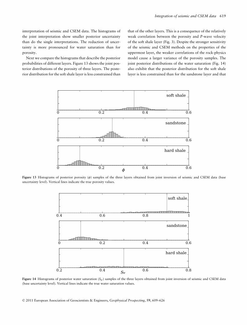
Next we compare the histograms that describe the posteriorprobabilities of different layers. Figure 13 shows the joint pos-terior distributions of the porosity of three layers. The poste-rior distribution for the soft shale layer is less constrained than

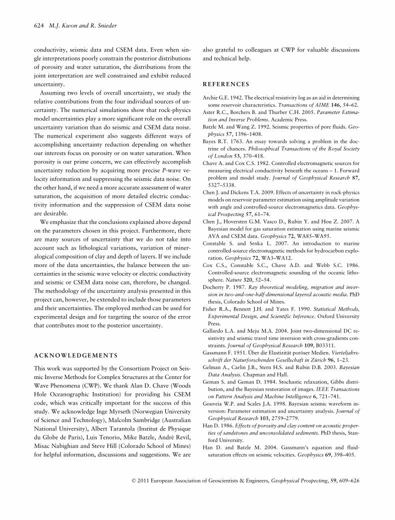
that of the other layers. This is a consequence of the relativelyweak correlation between the porosity and P-wave velocityof the soft shale layer (Fig. 3). Despite the stronger sensitivityof the seismic and CSEM methods on the properties of theuppermost layer, the weaker correlations of the rock-physicsmodel cause a larger variance of the porosity samples. Thejoint posterior distributions of the water saturation (Fig. 14)also exhibit that the posterior distribution for the soft shalelayer is less constrained than for the sandstone layer and that

Figure 13 Histograms of posterior porosity (φ) samples of the three layers obtained from joint inversion of seismic and CSEM data (baseuncertainty level). Vertical lines indicate the true porosity values.

Figure 14 Histograms of posterior water saturation (Sw) samples of the three layers obtained from joint inversion of seismic and CSEM data(base uncertainty level). Vertical lines indicate the true water saturation values.



the rock-physics model uncertainty has more significance onconstraining the posterior distribution than the resolution ofthe seismic and CSEM methods.

Finally, we study two representative uncertainty levels: abase state and a new state with reduced data uncertainties(Table 2). Note that the uncertainty of the electric conduc-tivity is defined on a logarithmic scale. The seismic data un-certainty is defined as a ratio from the maximum amplitudevalue and the CSEM data uncertainty is defined as a sum ofsystematic and non-systematic noise. Figures 13 and 14 rep-resent the posterior probability for the base uncertainty level.

The histograms for the reduced uncertainty level are shownin Figs 15 and 16. The reduced uncertainty level leads, ofcourse, to a sharper posterior probability distribution thanthe base state and thus increases the accuracy in the estimatesof porosity and water saturation. This stronger constraint ismore obvious for porosity than for water saturation. This isdue to the smaller resolution of the CSEM method comparedto the seismic method.

The correlation of reservoir parameters between differ-ent layers can be studied by cross-plot analysis. An exam-ple of a cross-plot analysis is shown in Fig. 17, where the

Figure 15 Histograms of posterior porosity (φ) samples of the three layers obtained from joint inversion of seismic and CSEM data (reduceduncertainty level). Vertical lines indicate the true porosity values.

Figure 16 Histograms of posterior water saturation (Sw) samples of the three layers obtained from joint inversion of seismic and CSEM data(reduced uncertainty level). Vertical lines indicate the true water saturation values.



Figure 17 Cross-plot of posterior water saturation samples of thesoft shale and sandstone layers. The histograms of the correspondingsamples are shown in Fig. 16. The vertical and horizontal lines indicatethe true water saturation values. The correlation coefficient betweenthe two random variables is negative (dashed line).

posterior water saturation samples of the soft shale and sand-stone layers are cross-plotted. The example demonstrates thatthe water saturation of the two layers has a negative corre-lation, which arises from the weak depth resolution of theCSEM exploration. Therefore, the correlation between thetwo layers becomes weaker as the thickness of the sandstonelayer increases. The weaker correlation of a reservoir param-eter between different layers generally accompanies reduceduncertainty of the reservoir parameter. The correlation anal-ysis can help diagnose the trade-off between different modelparameters.

Different scenarios for uncertainty reduction

In the previous section, we presented histograms that charac-terize the posterior uncertainty. As stated before, we assumethe multivariate Gaussian distribution (equation (4)) for thecalculation of prior and likelihood. There are however severalfactors that make the distribution of the posterior samplesnon-Gaussian. First, the porosity or water saturation has val-ues between 0–1. Second, the porosity sampling is bounded bythe critical porosity φc. The critical porosity is the thresholdvalue between the suspension and the load-bearing domain

and denotes the upper porosity limit of the range where therock-physics model can be applied (Mavko et al. 1998). Thecritical porosity values we apply for the soft shale, sandstoneand hard shale layer are 0.6, 0.4, and 0.4, respectively. Thesebounds can lead to skewed sample distributions. Furthermorethe posterior distributions do not necessarily follow the Gaus-sian distribution because of the non-linearity of the forwardmodels. The posterior uncertainty can generally be assessed bysample mean and sample variance. For reasons of clarity, weuse the Gaussian curves for the representation of the samplemean and sample variance.

In this project, we model four factors of uncertainty: rock-physics model uncertainties of the P-wave velocity and elec-tric conductivity and noise of the seismic and CSEM data.We discussed the posterior probabilities of the porosity andwater saturation for the base and reduced uncertainty levels(Table 2) in the previous section (Figs 13–16). We performthe following numerical experiments to quantify the contri-butions of the four possible sources of uncertainty. The initialsimulation is performed based on the base uncertainty level.For analysis of the contributions of each of the factors on theposterior uncertainties, six subsequent simulations are per-formed with reduced uncertainty levels of one or two of thefour factors of uncertainty. We perform the last simulationbased on reduced uncertainty levels of all factors of uncer-tainty (reduced level). These eight numerical experiments aresummarized in Table 3. We compare the posterior distribu-tions from different treatments with the base and reducedlevels and deduce how much a treatment contributes to theoverall change of the sample variances. The posterior distri-butions of the porosity and water saturation are shown inFigs 18–23.

Table 3 Eight numerical experiments for the analysis of the contribu-tions of four possible factors of uncertainty. Two states of uncertaintyfor the individual factors are listed in Table 2.

Uncertainty of the individual factors

Base level None of the factors are reducedTreatment-1 Only reducing P-wave velocity uncertaintyTreatment-2 Only reducing electric conductivity uncertaintyTreatment-3 Only reducing seismic noise levelTreatment-4 Only reducing CSEM noise levelTreatment-5 Reducing P-wave velocity uncertainty

and seismic noise levelTreatment-6 Reducing electric conductivity uncertainty

and CSEM noise levelReduced level Reducing all of the four uncertainty factors



Figure 18 Posterior probability distributions of porosity φ of thesandstone layer. The distributions from treatments 1 and 2 (Table3) are compared with those from the base and reduced levels. Verticalline indicates the true porosity value.

Figure 19 Posterior probability distributions of water saturation Sw

of the sandstone layer. The distributions from treatments 1 and 2(Table 3) are compared with those from the base and reduced levels.Vertical line indicates the true water saturation value.









Figures 18 and 19 show the posterior probability distribu-tions acquired after performing the treatments 1 and 2. Whenwe reduce uncertainty levels of the P-wave velocity or elec-tric conductivity, the resultant posterior distributions exhibitsmaller sample variances than the base level. Furthermore,the sample means are generally closer to the modelled valuesas we reduce the individual uncertainty levels. The proba-bility density distribution for the porosity of the sandstonelayer (Fig. 18) reveals that the P-wave velocity uncertaintyplays a significant role on the overall uncertainty reductionof the porosity and the contribution of the electric conductiv-ity uncertainty is limited. In contrast, Fig. 19 shows that theoverall uncertainty variation of the water saturation is morestrongly influenced by the uncertainty of the electric conduc-tivity than by the uncertainty of the P-wave velocity. This isconsistent with the simulated rock-physics models shown inFigs 3–6. From the rock-physics models, we can deduce thatthe porosity strongly influences both the P-wave velocity andelectric conductivity. The rock-physics models also show thatthe water saturation strongly influences the electric conduc-tivity while its influence on the P-wave velocity is limited.

The posterior probability distributions for treatments 3 and4 are shown in Figs 20 and 21. When we reduce the noise lev-els of the seismic or CSEM data, the improvements of theposterior uncertainties of the porosity and water saturationare much less significant than the improvements due to the re-duction of rock-physics model uncertainties. This shows thatthe overall uncertainty of the porosity and water saturation ismore influenced by the rock-physics model uncertainties thanby the noise of the seismic or CSEM data. The figures alsoshow that for the given range of data noise, the seismic datanoise reduction yields a more precise estimate than when theCSEM data noise is reduced.

Figures 22 and 23 show the posterior probability distribu-tions for treatments 5 and 6. Compared to the single improve-ment cases, it is clear that the combined improvements givebetter assessments about the porosity and water saturation.The probability density distributions shown in Figs 22 and 23are similar to the distributions shown in Figs 18 and 19. Thisimplies that the posterior uncertainty variations from the com-bined improvements are mainly governed by the improvementof rock-physics model uncertainties and the contributions ofthe seismic and CSEM data noise are less significant.

The posterior probability distributions shown in Figs 18–23are summarized in Table 4. The comparison of the variancevalues clearly show that the reductions of the sample vari-ances of the porosity and water saturation are most stronglyinfluenced by the uncertainty of the P-wave velocity and elec-

Table 4 Sample variances S2 of porosity φ andwater saturation Sw of the sandstone layer. Thedetails about the treatments are in Table 3.

Sample variance (× 10−3) S2 (φ) S2 (Sw)

Base level 0.560 1.997Treatment-1 0.041 1.456Treatment-2 0.516 0.205Treatment-3 0.501 1.865Treatment-4 0.532 1.728Treatment-5 0.039 1.251Treatment-6 0.498 0.198Reduced level 0.038 0.117

tric conductivity, respectively. The contributions of the rock-physics model uncertainties on the posterior uncertainties aregenerally larger than those of the seismic and CSEM datanoise. The numerical experiments suggest different ways ofaccomplishing uncertainty reduction depending on whetherour interests focus on the porosity or water saturation. Whenporosity is our prime concern, we can effectively accomplishuncertainty reduction by improving the P-wave velocity modeland by suppressing the seismic data noise. On the other hand,if we need a more accurate assessment of water saturation, theacquisition of more detailed electric conductivity informationand the suppression of CSEM data noise are preferred.

Note that the above assessments are based on marginalanalysis of posterior probability, and a possible correlationbetween different uncertainty factors is ignored. This can bemisleading in the presence of strong correlation. The correla-tion between uncertainty factors can be analysed by the fullfactorial experiment (Fisher, Bennett and Yates 1990) that re-quires 2n treatments, where n is the number of uncertaintyfactors.

CONCLUSIONS

We have shown that the posterior probability random sam-pling based on the Metropolis-Hastings algorithm is capableof assessing the multi-dimensional probability distribution ofporosity and water saturation. We have also shown that thejoint inversion of the seismic and CSEM data can be achievedby introducing rock-physics models that interconnect the P-wave velocity and electric conductivity. There are four rep-resentative sources of uncertainty that influence the posteriorprobability density of porosity and water saturation. Theseuncertainties are related to seismic wave velocity, electric



conductivity, seismic data and CSEM data. Even when sin-gle interpretations poorly constrain the posterior distributionsof porosity and water saturation, the distributions from thejoint interpretation are well constrained and exhibit reduceduncertainty.

Assuming two levels of overall uncertainty, we study therelative contributions from the four individual sources of un-certainty. The numerical simulations show that rock-physicsmodel uncertainties play a more significant role on the overalluncertainty variation than do seismic and CSEM data noise.The numerical experiment also suggests different ways ofaccomplishing uncertainty reduction depending on whetherour interests focus on porosity or on water saturation. Whenporosity is our prime concern, we can effectively accomplishuncertainty reduction by acquiring more precise P-wave ve-locity information and suppressing the seismic data noise. Onthe other hand, if we need a more accurate assessment of watersaturation, the acquisition of more detailed electric conduc-tivity information and the suppression of CSEM data noiseare desirable.

We emphasize that the conclusions explained above dependon the parameters chosen in this project. Furthermore, thereare many sources of uncertainty that we do not take intoaccount such as lithological variations, variation of miner-alogical composition of clay and depth of layers. If we includemore of the data uncertainties, the balance between the un-certainties in the seismic wave velocity or electric conductivityand seismic or CSEM data noise can, therefore, be changed.The methodology of the uncertainty analysis presented in thisproject can, however, be extended to include those parametersand their uncertainties. The employed method can be used forexperimental design and for targeting the source of the errorthat contributes most to the posterior uncertainty.

ACKNOWLEDGEME N T S

This work was supported by the Consortium Project on Seis-mic Inverse Methods for Complex Structures at the Center forWave Phenomena (CWP). We thank Alan D. Chave (WoodsHole Oceanographic Institution) for providing his CSEMcode, which was critically important for the success of thisstudy. We acknowledge Inge Myrseth (Norwegian Universityof Science and Technology), Malcolm Sambridge (AustralianNational University), Albert Tarantola (Institut de Physiquedu Globe de Paris), Luis Tenorio, Mike Batzle, Andre Revil,Misac Nabighian and Steve Hill (Colorado School of Mines)for helpful information, discussions and suggestions. We are

also grateful to colleagues at CWP for valuable discussionsand technical help.

REFERENCES

Archie G.E. 1942. The electrical resistivity log as an aid in determiningsome reservoir characteristics. Transactions of AIME 146, 54–62.

Aster R.C., Borchers B. and Thurber C.H. 2005. Parameter Estima-tion and Inverse Problems. Academic Press.

Batzle M. and Wang Z. 1992. Seismic properties of pore fluids. Geo-physics 57, 1396–1408.

Bayes R.T. 1763. An essay towards solving a problem in the doc-trine of chances. Philosophical Transactions of the Royal Societyof London 53, 370–418.

Chave A. and Cox C.S. 1982. Controlled electromagnetic sources formeasuring electrical conductivity beneath the oceans – 1. Forwardproblem and model study. Journal of Geophysical Research 87,5327–5338.

Chen J. and Dickens T.A. 2009. Effects of uncertainty in rock-physicsmodels on reservoir parameter estimation using amplitude variationwith angle and controlled-source electromagnetics data. Geophys-ical Prospecting 57, 61–74.

Chen J., Hoversten G.M. Vasco D., Rubin Y. and Hou Z. 2007. ABayesian model for gas saturation estimation using marine seismicAVA and CSEM data. Geophysics 72, WA85–WA95.

Constable S. and Srnka L. 2007. An introduction to marinecontrolled-source electromagnetic methods for hydrocarbon explo-ration. Geophysics 72, WA3–WA12.

Cox C.S., Constable S.C., Chave A.D. and Webb S.C. 1986.Controlled-source electromagnetic sounding of the oceanic litho-sphere. Nature 320, 52–54.

Docherty P. 1987. Ray theoretical modeling, migration and inver-sion in two-and-one-half-dimensional layered acoustic media. PhDthesis, Colorado School of Mines.

Fisher R.A., Bennett J.H. and Yates F. 1990. Statistical Methods,Experimental Design, and Scientific Inference. Oxford UniversityPress.

Gallardo L.A. and Meju M.A. 2004. Joint two-dimensional DC re-sistivity and seismic travel time inversion with cross-gradients con-straints. Journal of Geophysical Research 109, B03311.

Gassmann F. 1951. Uber die Elastizitat poroser Medien. Vierteljahrs-schrift der Naturforschenden Gesellschaft in Zurich 96, 1–23.

Gelman A., Carlin J.B., Stern H.S. and Rubin D.B. 2003. BayesianData Analysis. Chapman and Hall.

Geman S. and Geman D. 1984. Stochastic relaxation, Gibbs distri-bution, and the Bayesian restoration of images. IEEE Transactionson Pattern Analysis and Machine Intelligence 6, 721–741.

Gouveia W.P. and Scales J.A. 1998. Bayesian seismic waveform in-version: Parameter estimation and uncertainty analysis. Journal ofGeophysical Research 103, 2759–2779.

Han D. 1986. Effects of porosity and clay content on acoustic proper-ties of sandstones and unconsolidated sediments. PhD thesis, Stan-ford University.

Han D. and Batzle M. 2004. Gassmann’s equation and fluid-saturation effects on seismic velocities. Geophysics 69, 398–405.



Harris P. and MacGregor L. 2006. Determination of reservoir prop-erties from the integration of CSEM and seismic data. First Break24, 53–59.

Hastings W.K. 1970. Monte Carlo sampling methods using MarkovChains and their applications. Biometrika 57, 97–109.

Hoversten G.M., Cassassuce F., Gasperikova E., Newman G.A., ChenJ., Rubin Y. et al. 2006. Direct reservoir parameter estimation usingjoint inversion of marine seismic AVA and CSEM data. Geophysics71, C1–C13.

Hu W., Abubakar A. and Habashy T. 2009. Joint electromagneticand seismic inverion using structural contraints. Geophysics 74,R99–R109.

Jannane M., Beydoun W., Crase E., Cao D., Koren Z., Landa E. et al.1989. Wavelengths of earth structures that can be resolved fromseismic reflection data. Geophysics 54, 906–910.

Kaipio J.P., Kolehmainen V., Somersalo E. and Vauhkonen M. 2000.Statistical inversion and Monte Carlo sampling methods in electri-cal impedance tomography. Inverse Problems 16, 1487–1522.

Mavko G., Mukerji T. and Dvorkin J. 1998. The Rock Physics Hand-book. Cambridge University Press.

Metropolis N., Rosenbluth A.W., Rosenbluth M.N. and Teller A.H.1953. Equation of state calculations by fast computing machines.The Journal of Chemical Physics 21, 1087–1092.

Mosegaard K. and Sambridge M. 2002. Monte Carlo analysis ofinverse problems. Inverse Problems 18, R29–R54.

Mosegaard K., Singh S., Snyder D. and Wagner H. 1997. Monte Carloanalysis of seismic reflections from Moho and the W reflector.Journal of Geophysical Research 102, 2969–2981.

Musil M., Maurer H.R. and Green A.G. 2003. Discrete tomographyand joint inversion for loosely connected or unconnected physicalproperties – Application to crosshole seismic and georadar datasets. Geophysical Journal International 153, 389–402.

Palacky G.J. 1987. Resistivity characteristics of geologic targets.In: Electromagnetic Methods in Applied Geophysics (ed. M.N.Nabighian), pp. 53–129. SEG.

Revil A., Cathles L.M. and Losh S. 1998. Electrical conductivity inshaly sands with geophysical applications. Journal of GeophysicalResearch 103, 23925–23936.

Sambridge M., Beghein C., Simons F.J. and Snieder R. 2006. How dowe understand and visualize uncertainty?. The Leading Edge 25,542–546.

Scales J.A. and Tenorio L. 2001. Prior information and uncertaintyin inverse problems. Geophysics 66, 389–397.

Snieder R., Xie M.Y., Pica A. and Tarantola A. 1989. Retrieving boththe impedance contrast and background velocity – A global strategyfor the seismic reflection problem. Geophysics 54, 991–1000.

Spikes K., Mukerji T., Dvorkin J. and Mavko G. 2007. Probabilisticseismic inversion based on rock-physics models. Geophysics 72,R87–R97.

Tarantola A. 2005. Inverse Problem Theory and Methods for ModelParameter Estimation. Society for Industrial and Applied Mathe-matics.

Tenorio L. 2001. Statistical regularization of inverse problems. SIAMReview 43, 347–366.

Tikhonov A.N. and Arsenin V.Y. 1977. Solution of Ill-posed Prob-lems. Winston and Sons.

Ulrych T.J., Sacchi M.D. and Woodbury A. 2001. A Bayes tour ofinversion – A tutorial. Geophysics 66, 55–69.

Waxman M.H. and Smits L.J.M. 1968. Electrical conductivities inoil-bearing shaly sands. Society of Petroleum Engineering Journal8, 107–122.

Wood A.W. 1955. A Textbook of Sound. The MacMillan Co.Yilmaz O. 1987. Seismic Data Processing. SEG.

APPENDIX A: METROPOLIS -HASTINGSALGORITHM

The Metropolis-Hastings algorithm (Metropolis et al. 1953;Hastings 1970) is a method for generating a sequence of sam-ples from a probability distribution that is difficult to sampledirectly. The actual implementation of the algorithm is com-prises of the following steps.

1 Pick an initial sample mprev ∈ Rn and set k = 1, m(k) = mprev.

2 Set k → k + 1.3 Draw a proposal sample mprop ∈ R

n from the proposal dis-tribution q(mprev, mprop) and calculate the acceptance ratio

α(mprev, mprop) = min[1,

πpost(mprop)q(mprop, mprev)πpost(mprev)q(mprev, mprop)

].

(A1)

4 Draw t ∈ [0, 1] from the uniform probability density.5 If α(mprev, mprop) ≥ t, set m(k) = mprop; otherwise, m(k) =mprev.6 When k is the desired sample size, stop; otherwise, repeatthe procedure starting with step (2).

We choose a Gaussian distribution as a proposal distributionas follows:

mprop ∼ N(mprev, σ

2i I

), (A2)

where the variances σ 2i describe the probabilistic sampling step

of the model parameters during the random simulation. If σ 2i

is too large, the drawn mprop is practically never accepted. Onthe other hand, if σ 2

i is too small, a proper sampling of thedistribution requires a prohibitively large sample set. A goodrule of thumb is that roughly 20–30% of all mprop should beaccepted (Kaipio et al. 2000).



APPENDIX B: ROCK-PHYSICS MODELSOF THIS STUDY

P-wave velocity Vp is defined as a function of bulk modulusK, shear modulus μ and density ρ, such that

Vp =√

K + 43 μ

ρ. (B1)

The bulk modulus K is related to porosity φ and water sat-uration Sw. For a fluid saturated medium, the bulk modulusis given by Gassmann’s equation (Gassmann 1951; Han andBatzle 2004) as follows:

K = Kd +(1 − Kd

K0

)2

φ

K f+ 1−φ

K0− Kd

K20

, (B2)

where Kd, K0 and Kf are the bulk modulus of the dry rock,mineral material and pore fluid, respectively. We model twophases of pore fluid: water and gas. A mixture of two differentpore fluids can be regarded as an effective fluid model and thebulk modulus is derived from Wood’s equation (Wood 1955;Batzle and Wang 1992) as follows:

1K f

= Sw

Kw

+ 1 − Sw

Kg, (B3)

where Kw and Kg are the bulk modulus of the water and gasphases. We also relate the bulk modulus of the dry rock Kd

and shear modulus μ with porosity φ as follows:

Kd = K0

(1 − φ

φc

), (B4)

μ = μ0

(1 − φ

φc

), (B5)

where μ0 is the shear modulus of the mineral material andφc is the critical porosity that is the threshold porosity value

between the suspension and the load-bearing domain. Finally,we model the dependence of density ρ on porosity and watersaturation as:

ρ = φSwρw + (1 − φ)ρ0, (B6)

where ρw and ρ0 are the density of water phase and mineralmaterial, respectively.

The relationship between the reservoir parameters and elec-tric conductivity is first given by Archie’s second law (Archie1942), which describes electric conductivity in clean sands. Infact, electric conductivity in shaley sands is complicated bythe presence of clays and is described by the Waxman-Smitsformula (Waxman and Smits 1968):

σe = φmSnw

[σw + BQv

Sw

], (B7)

where m is the cementation exponent, n is the saturation ex-ponent and σ w is electric conductivity of the pore fluid. Theparameter B is an equivalent counterion mobility and Qv isthe excess of surface charge per unit pore volume. ParameterB is given empirically at 25◦C by

B = B0

[1 − 0.6 exp

(− σw

0.013

)], (B8)

where σ w is in S/m and the maximum counterion mobilityB0 is given by 4.78 × 10−8 m2/V/s (Revil, Cathles and Losh1998). Parameter Q is related to the mineral density ρ0 (inkg/m3) and the cation exchange capacity (CEC) by

Qv = ρ01 − φ

φCEC. (B9)

The cation exchange capacity is only significant for clay miner-als and the variation of cation exchange capacity for differentclay minerals is dramatic.

The modelled values of each rock-physics parameters intro-duced above are summarized in Table 1.


uncertainty analysis for the integration of seismic and...

Documents