uncertainty analysis review · 2017-11-06 · storage reservoir stormwater treatment areas (stas)...

Uncertainty Analysis Review

Alaa Ali, PhD, PE, PMP, DWRE

Principal Engineer

Hydrologic and Environmental Systems Modeling

South Florida Water Management District

PRESENTATION HIGHLIGHTS

Introduction to SFWMD including CERP

SFWMD primary models

Previous workshops on UA

Uncertainty Analysis and Sensitivity Analysis Basic definition

Sources and measures of uncertainty

Uncertainty Analysis techniques

Application to NSRSM to demonstrate the following:

• Local sensitivity analysis

• Global sensitivity analysis

• Uncertainty Analysis techniques

• Global Sensitivity Analysis

Conclusion and lessons learned

SFWMD Mission

To manage and protect

water resources of the

region by balancing and

improving water quality,

flood control, natural

systems and water supply

Coastal Watersheds & Estuaries

Everglades

Kissimmee

Lake Okeechobee

Mange Drought & Floods

Provide Water Supply

Protect & Restore Ecosystems

Prepare for Emergencies

Science, Planning, Engineering, & Construction

Land Management

Operation & Maintenance

Regulation

Water Supply Development

Objectives

Jan

Feb Mar

Apr

May

Jun

Jul

Aug

Sep

Oct

Nov

Dec

0

5

10

15

20

25

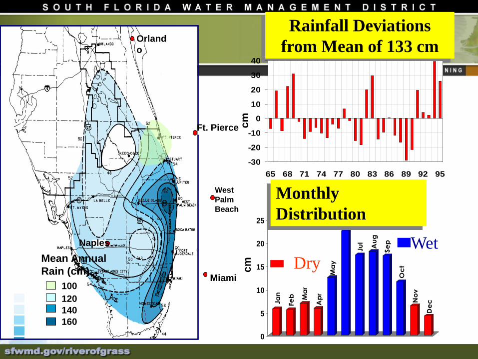
Monthly

Distribution

Wet

Drycm

Rainfall Deviations

from Mean of 133 cm

-30

-20

-10

0

10

20

30

40

65 68 71 74 77 80 83 86 89 92 95

cm

Mean Annual

Rain (cm)

100

120

140

160

Orland

o

Ft. Pierce

West

Palm

Beach

Miami

Naples

Soil Subsidence

Pre-drainage

Post-drainage

EAA Water Conservation

Areas

Lake O

Current

Flow

Our

Ecosystem

has been

altered

dramatically

Orlando

Florida Bay

Big Cypress

National

Preserve

Ft. Myers

Okeechobee

WCAs

Lake

CERP

Components

Everglades

National

Park

Aquifer

Storage

& Recovery

Surface Water

Storage Reservoir

Stormwater

Treatment Areas

(STAs)

Reuse Wastewater

Seepage

Management

Removing Barriers

to Sheetflow

Operational

Changes

• 6 pilot projects

• 15 surface storage areas(~170,000 acres)

• 3 in-ground reservoirs(~11,000 acres)

• 19 stormwatertreatment areas (~36,000 acres)

• 330 aquifer storage and recovery wells

• 2 wastewater reuse plants

• Removal of over 240 miles ofcanals, leveesand structures

• Operational changes

Major C&SF Project Components

River Channelization

Herbert Hoover Dike

Water Conservation Areas

Protective Levees

• Everglades Agricultural Area

• Lower East Coast

Drainage Network

• Salinity Structures

What is a MODEL?

Input data at limited

sites in space/time

Mathematical representation

of the system processes and

Numerical implementation

System's

parameters &

BC measured at

limited points

Management

Decisions

Prediction

Integrated surface water groundwater model

Regional-scale 3.2 x 3.2 km, daily time step

Major components of hydrologic cycle

Overland and groundwater flow

Canal and levee seepage

Operations of C&SF system

Water shortage policies

Extensive performance measures

Provides input and boundary conditions for other models

South Florida Water Management Model (SFWMM)

www.sfwmd.gov/org/pld/hsm/models

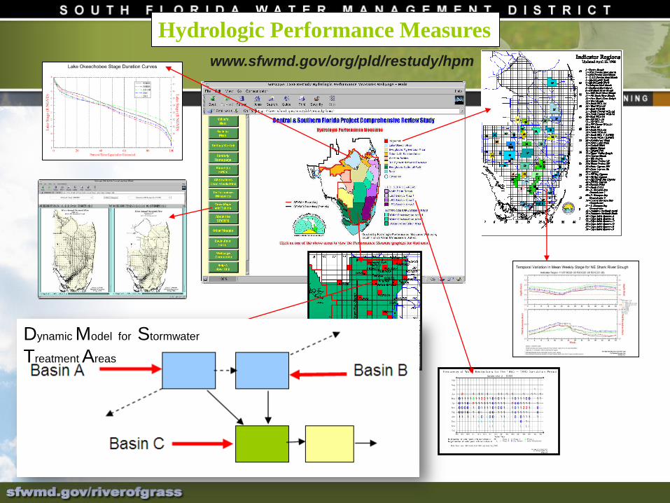
Hydrologic Performance Measures

www.sfwmd.gov/org/pld/restudy/hpm

Dynamic Model for Stormwater

Treatment Areas

RSM

Hydrologic Simulation

Engine (HSE)

Management Simulation

Engine (MSE)

RSM Engines

South Florida Regional Simulation Model

SFRSM

• Model physical setup

• Simulate hydrologic

processes

• Overland flow

• Groundwater flow

• Canal network

• Calibration/validation

of model parameters

• Use observed

structure flows

• Simulate structure

operations

• Implementation of

operational rules

• Flood control rules

• Water supply policies

• Maintain minimum

flows & levels

• Regional operational

coordination

Numerical Mesh

5,794 triangular cells

Mean & standard deviation of mesh cell sizes: 1.01 mi2 & 0.74 mi2

Mesh cell size range: 0.05 mi2 to 3.92 mi2

WCA-3B has the finest resolution; BCNP has the coarsest resolution

WCA-3A has a total of 984cells

Average cell size in WCA-3Ais 0.79 mi2; standard deviation is 0.24 mi2

0 9 18 27 36

Miles

Legend

Structure

Canals

Basins

Mesh

Model Boundary

Previous Workshops at SFWMD

January 18-19, 1994 Workshop on Reduction of Uncertainties in Regional Hydrologic Simulation Models produced a report:

• Sensitivity and Uncertainty Analysis in Hydrologic Simulation Modeling of the South Florida Water Management District Daniel P. Loucks and Jery R. Stedinger March 1, 1994

August 1995: An evaluation of the certainty of system performance measures generated by the South Florida Water Management Model Paul J. Trimble.

January 15-17, 2002: MODEL UNCERTAINTY WORKSHOP produced a report

• Quantifying and Communicating Model Uncertainty for Decision Making in the Everglades Upmanu Lall, Donald L. Phillips, Kenneth H. Reckhow and Daniel P. Loucks May 2002

September 24, 2004: Uncertainty Workshop, Interagency Modeling Center : Presented by Christine Shoemaker, Jack Gwo and Wasantha Lal

May 2005: Interagency Modeling Center Calculating MODFLOW Analytical Sensitivities Using ADIFOR for Effective and Efficient Estimation of Uncertainties Amir Gamliel, Mike Fagan and Maged Hussein

August 2005: Interagency Modeling Center : Uncertainty of A Remediation Cost: A Demonstration of the NLH Technique in the analysis of uncertainty of objective value in model application Jack Gwo and George Shih

Bias, Precision, and Total Error

Bias Error

Total Error

Precision

Error

H True H simulated

It determines the probability distribution of entire set of

possible outcomes by considering the uncertainties in

model input, parameters and algorithm.

As it pertains to SFWMM/RSM, UA is a procedures of

mapping uncertainty bands of model

input/parameters/structure to uncertainty bands of

model outcomes (prediction).

Uncertainty Analysis (UA)

Uncertainty Analysis (UA)Sensitivity Analysis (SA), definition

• A procedure to determine the sensitivity of model

outcomes to changes in its parameters. If a small

change in a parameter results in relatively large

changes in the outcomes, the outcomes are said to be

sensitive to that parameter.

To understand which parameters are most critical for

the model output

• To estimate parameter maximum and minimum values

that provide plausible model outcomes for the purpose

of providing some information about the parameter

uncertainty.

• To calculate sensitivity matrix (Jacobian) which is a

requirement for uncertainty analysis techniques.

Uncertainty Analysis (UA)Sensitivity Analysis (SA), purpose

Is the investigation of the combined effect of input uncertainty and the input/output sensitivity on the output uncertainty.

Is the Isolation of the input parameters with most contribution to model output variance.

Function of input uncertainty and output sensitivity to that input

IA techniques:

• Stepwise Rank Regression Analysis

• Classification Tree Analysis

Uncertainty Analysis (UA)Importance Analysis (IA), OR Global Sensitivity Analysis

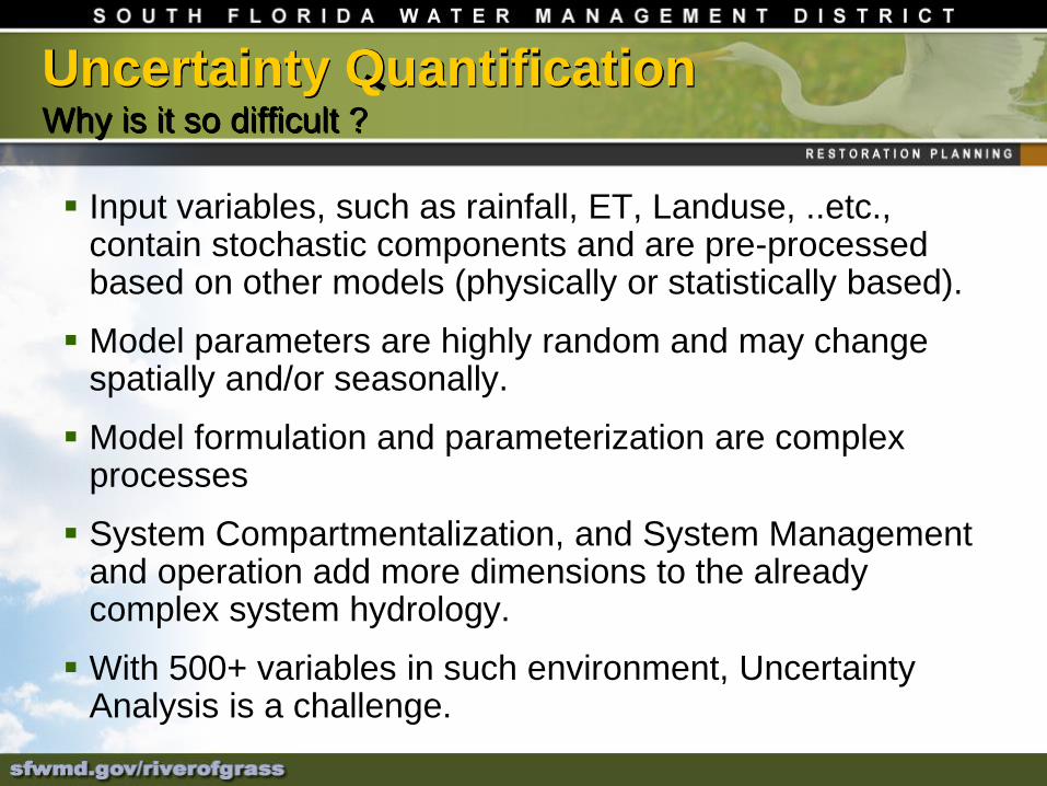
Input variables, such as rainfall, ET, Landuse, ..etc., contain stochastic components and are pre-processed based on other models (physically or statistically based).

Model parameters are highly random and may change spatially and/or seasonally.

Model formulation and parameterization are complex processes

System Compartmentalization, and System Management and operation add more dimensions to the already complex system hydrology.

With 500+ variables in such environment, Uncertainty Analysis is a challenge.

Uncertainty QuantificationWhy is it so difficult ?

Uncertainty due to our inability to fully understand

the natural variability of input process to the

model at a scale smaller than the gauging scale.

Examples of these uncertainties are:

• Spatial variability such as rainfall, PET, and topography

• Temporal variability such as inflow and tidal boundary

conditions

Sources of Uncertainty

SOURCES OF UNCERTAINTY, cont.

Uncertainty due to measurement errors. This

covers all field measurements and published data

based on which input and output data are directly

used, or estimated using an external data

processing (or modeling).

Uncertainty due to conceptual and implementation

errors :-

• Error in specifying boundary conditions such as inflow

and tidal boundaries and initial conditions such as stage.

• Model structural and numerical errors

SOURCES OF UNCERTAINTY, cont.

Conceptual and implementation errors (cont.)

• Model parameter errors due to parameter modeling errors

and/or calibration imperfection.

• Model inability to resolve variability smaller than the

designated time step and mesh cell size

• Temporal and spatial discretizations and their

interdependence

Model linkage to other models

• Water quality and hydrologic model integration/coupling

• Input preprocessing models (demands, runoffs, rainfall, ..etc.

MEASURES AND SOME USES OF

UNCERTAINTY

In its simple format, a mean and a standard deviation of a given

output, performance measure or index. This simplified

uncertainty metric is rarely sufficient for a complete

characterization of uncertainty.

Model output in terms of a range rather than a single value. This

describes the system performance as a range of potential

outputs, classes of likely events, or probability density function.

Provides a level of confidence that a certain output is within an

acceptable performance indicators.

Provides probability that a certain output exceeds a specific

target value.

TECHNIQUES TO QUANTIFY

UNCERTAINTY

ANALYTICAL:

• Derive the output error distribution (e.g., variance)

• Feasible for simple models with few stochastic

(random) input parameters.

• Given the complexities and large variables in our

models, this approach does not go very far.


UNCERTAINTY

FIRST-ORDER SECOND MOMENT ANALYSES:

• This method derives the output variance from input parameter

variance / covariance functions

• This method can identify the relative contribution of each

parameter to the output variance.

• Suitable when parameter-output relationship is linear or mildly

nonlinear.

• If the linearity condition is not “properly” satisfied, then second

order term of Taylor expansion must be considered and a

correction term must be applied

• Refer to Loucks & Stedinger 1994, Trimble 1995, and Lal

1995.


UNCERTAINTY

)ˆ()ˆ()( ii

i i

xxx

FFF

xx

]])[[(][ 22 FFFV F EE

][])ˆ()ˆ[()( ji

jj ii

jjii

jj ii

xxCx

F

x

Fxxxx

x

F

x

FFV

E

][)(

2

i

i i

xVx

FFV

FIRST-ORDER SECOND MOMENT ANALYSES:


UNCERTAINTY

Stochastic Numerical Models:

• Develop and solve the governing equation with

stochastic component

• Probability distribution is inherent in the solution

• Very simple models compared to SFWMD system

• Numerical solution of such a stochastic equation is far

more complex than the already challenging solution of

the deterministic equation.


UNCERTAINTY

Monte Carlo with Random Sampling

• Recognize some input variables/parameters as random.

Identify their probability distributions by expert judgment and

historical data.

• For each simulation model run, draw the actual values of

input variables/parameters from their respective distribution.

Record the corresponding output.


UNCERTAINTY

Monte Carlo with Random Sampling (cont.)

• With considerable number of simulations and many recorded

outputs (all are equally likely outcomes), obtain output

probability distribution.

• Massive number of simulations is needed

• Input parameters/variables are likely correlated both in space

and time and hence sampling must be drawn from a joint

probability distribution that reflect both scales. The

construction of such distributions is not easy


UNCERTAINTY

Bayes’ Theorm

P(K) is the prior (marginal) probability of K (e.g., Hydraulic Conductivity).

P(K|Q) is the conditional (posterior) probability of K, given Q (e.g.,

Observed flow).

P(Q|K) is the conditional probability of Q given K. It is also called the

likelihood of K for observed Q. P(Q|K) ≈ L(K|Q). A measure of the

ability of “K” set in predicting the Observed “Q” set.

P(Q) is the prior or marginal probability of Q, and acts as a normalizing

constant.

Bayes' theorem in this form gives a mathematical representation of how

the conditional probability of event K given Q is related to the converse

conditional probability of Q given K.


UNCERTAINTY

Bayesian Monte Carlo analysis

• Combine prior information about the input parameter

distribution with the ability of these parameters to

describe available data on state variables.

• Start with the traditional Monte Carlo sampling from

prior distributions.

• Compare each simulation results to field

observations of the model state variables (e.g., flow)

and Score each results with respect to the ability of

each parameter set to describe the observed data.

•


UNCERTAINTY

Bayesian Monte Carlo analysis

• Scoring system can be as simple as yes/no binary

function or it can be based on a likelihood function

P(Q|K) ≈ L(K|Q).

• Perform sufficient simulations for the n parameters and

build n-dimensional matrix describing the marginal

parameter uncertainty and the entire error covariance

structure.

• You can do one of two things: define model prediction

uncertainty or investigate the parameter individual

contributions to overall uncertainty.

TECHNIQUES TO

QUANTIFY

UNCERTAINTY

Generalized Likelihood Uncertainty Estimation

Monte Carlo Markov Chain

DISADVANTAGE OF MONTE CARLO

TECHNIQUE

Large number of simulations is expensive

computationally especially for distributed models with

long run time

Risk of obtaining unrealistic combinations of input

values especially if the input variables/parameters are

NOT independent.

TECHNIQUES FOR COMPUTATION

EFFICIENCY

Latin Hypercube Sampling

• It reduces the number of input sampling variability

• For each input variable/parameter, the probability distribution is divided into segments of equal probability

• The algorithm assures sampling only once from each segment.

• Modification to this algorithm considers the variables/parameters interdependency

Latin hypercube sampling method

NSRSM UNCERTAINTY ANALYSIS

OBJECTIVES **

Considering a select group of parameters:

• Provide local sensitivity analysis

• Provide uncertainty analysis using more than one technique.

• Provide Global sensitivity analysis

STEPS**

1. Selection of a limited set of key inputs and outputs

based on previous modeling studies and expert

opinion.

2. Application of formal local sensitivity analysis (via

Singular Value Decomposition of the input-output

sensitivity matrix) to identify significant input

uncertainties.

3. Assignment of probability distributions to characterize

uncertainty in selected model inputs and their

correlation structure (based on the best available data).

STEPS (cont.)**

4. Application of uncertainty quantification techniques to

determine the uncertainty in model output (s) as a

function of the uncertainty in model inputs.

5. Application of global sensitivity (uncertainty

importance) analysis techniques to identify those

model inputs that are key contributors to the overall

uncertainty in model output(s). This results in an

importance ranking that is dependent on both input

uncertainty and input-output sensitivity, whereas the

importance ranking based on SVD factorization is only

dependent on input-output sensitivity.

1) Input/Output Selection

!(

!(

!(!(!(!(

!(

!(!(

!(!(

!(!(!(!(!(

!(!(!(!(!(!(!( !(!(!(!(!(!(!(!(!(!(!(!(!(!(!(!(!(!(!(!(

0 10 20 305Miles

25492

25087

NSRSM Model Boundary

Ridge and Slough Marsh

Mesic Pine Flatwood

Rivers

Tamiami Transect

T712_East Transect

Land cover types chosen for parameter variation and locations of output metrics.

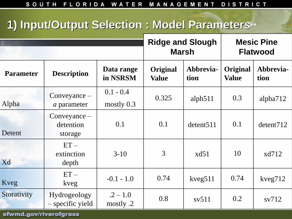
1) Input/Output Selection : Model Parameters**

Ridge and Slough

Marsh

Mesic Pine

Flatwood

Parameter DescriptionData range

in NSRSM

Original

Value

Abbrevia-

tion

Original

Value

Abbrevia-

tion

AlphaConveyance –

a parameter

0.1 - 0.4

mostly 0.30.325 alph511 0.3 alpha712

Detent

Conveyance –

detention

storage

0.1 0.1 detent511 0.1 detent712

Xd

ET –

extinction

depth

3-10 3 xd51 10 xd712

KvegET –

kveg-0.1 - 1.0 0.74 kveg511 0.74 kveg712

Storativity Hydrogeology

– specific yield

.2 – 1.0

mostly .20.8 sv511 0.2 sv712

Metric Type Location Abbreviation

Stage 25492, land cover 511 25492stage

Stage 25087, land cover 712 25087stage

Transect Flow land cover 511 Tamiami

Transect Flow land cover 712 T712_East

1) Input/Output Selection : Output Metric**

2) SVD-Based Local Sensitivity Analysis:

SVD Singular Value Decomposition**

Consider Sensitivity Matrix (Jacobian) AmXn , with an entry ai,j

αij = the sensitivity of the jth simulated output metric to the ith parameter

hj = the jth simulated output

ki = the ith parameter

m = # of observations, n = # of parameters

mjnik

h

i

j

ji ......,2,1........,...,2,1........,

a

Matrix A can be decomposed into three matrices V,

S, and U

S is a diagonal matrix of singular values of A (i.e., the value that makes the corresponding row of matrix A = 0.)

VT gives the coefficients of linear combinations of the original parameters that give rise to new, independent parameter groups

U gives the coefficients of linear combinations of the observation groups.

The parameter groups and observation groups are related by the diagonal matrix S

The relative magnitude of the singular values in S indicates the relative importance of each of the parameter groups

T

nxnmxnmxm VSUA ..

TVVR .

Other Important Matrices for Sensitivity

Analysis

Resolution Matrix gives insight

regarding parameter resolution

(parameter interdependence)

i

j

ijx

y

a

Correlation Matrix gives insight regarding parameter resolution (parameter interdependence)

jjii

ij

ji

TVSV

.,..)./1(

2

,

2

The singular values, U and VT, the resolution matrix, and the

correlation matrix are the primary sources of information used

to construct groups of parameters, understand their

interdependence, and analyze their sensitivity

RESULTS: SVD-BASED SENSITIVITY ANALYSIS

alp

ha511

alp

ha712

dete

nt5

11

dete

nt7

12

xd

511

xd

712

kveg

511

kveg

712

sv511

sv712

25492

25087

Tamiami

T712East

Bubble plot of the sensitivity matrix


Singular values from the SVD decomposition,

Cutoff to control data error: smin/smax < 0.001

RESULTS: SVD-BASED SENSITIVITY

ANALYSIS

U matrix elements showing linear coefficients of the output groups

RESULTS: SVD-BASED SENSITIVITY

ANALYSIS

Elements of the VT matrix showing linear coefficients of parameter groups


Bubble plot of the Resolution matrix

alp

ha511

alp

ha712

dete

nt5

11

dete

nt7

12

xd

511

xd

712

kveg

511

kveg

712

sv511

sv712

alpha511

alpha712

detent511

detent712

xd511

xd712

kveg511

kveg712

sv511

sv712


Bubble plot of the Correlation matrix

alp

ha511

alp

ha712

dete

nt5

11

dete

nt7

12

xd

511

xd

712

kveg

511

kveg

712

sv511

sv712

alpha511

alpha712

detent511

detent712

xd511

xd712

kveg511

kveg712

sv511

sv712

3) CHARACTERIZATION OF

PARAMETER UNCERTAINTY

Ridge and Slough

Marsh (.325)

Mesic Pine Flatwood

(.3)

Value CDF

.06 0

.3 .15

.35 .95

.4 1

Value CDF

.3 0

.35 .10

.45 .90

.6 1

Manning’s n

Ridge and Slough

Marsh (.1)

Mesic Pine Flatwood

(.1)

Value CDF

.1 0

.6 1

Value CDF

.1 0

.2 1

Detention Storage

Conveyance

Ridge and Slough

Marsh (.88)

Mesic Pine Flatwood

(.84)

Value CDF

.7 0

.8 .5

.9 1.0

Value CDF

.4 0

.6 .40

.7 .90

.8 1

Vegetation Crop Coefficient

Ridge and Slough

Marsh (3.0)

Mesic Pine Flatwood

(10.0)

2-4 Normal

Distribution

3.0 mean .33

standard dev.

8-12 Normal

Distribution

10.0 mean 0.667

stand dev

Extinction Depth

ET

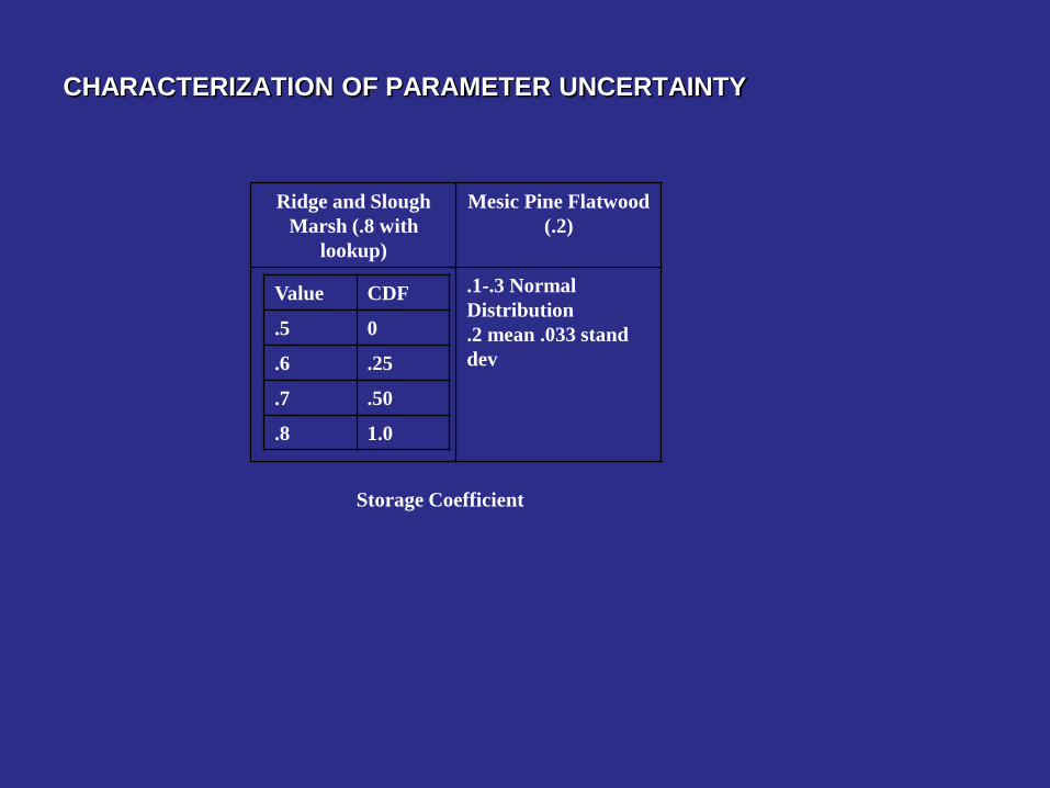
CHARACTERIZATION OF PARAMETER UNCERTAINTY

Ridge and Slough

Marsh (.8 with

lookup)

Mesic Pine Flatwood

(.2)

.1-.3 Normal

Distribution

.2 mean .033 stand

dev

Value CDF

.5 0

.6 .25

.7 .50

.8 1.0

Storage Coefficient

4) UNCERTAINTY Quantification:

Monte Carlo Simulation

First Order Second Moment Analysis

UNCERTAINTY PROPAGATION **:Comparison of MCS and FOSM results.

FOSM MCS

Mean Stdev Mean Stdev

25492stage 1.26 0.12 1.26 0.14

24087stage 0.13 0.054 0.13 0.047

Tamiami 2.55E+08 3.25E+07 2.70E+08 7.86E+07

T712_East -8.49E+07 9.80E+06 -8.25E+07 1.13E+07

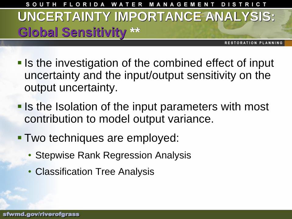
UNCERTAINTY IMPORTANCE ANALYSIS:

Global Sensitivity **

Is the investigation of the combined effect of input uncertainty and the input/output sensitivity on the output uncertainty.

Is the Isolation of the input parameters with most contribution to model output variance.

Two techniques are employed:

• Stepwise Rank Regression Analysis

• Classification Tree Analysis


Stepwise Rank Regression Analysis

Fit a linear response surface between the rank-transformed input and output variables and Perform a sensitivity analysis on this “surrogate” model.

Include variables to the regression in a stepwise fashion. The order by which variables are added to the regression model corresponds to their order of importance.

The order of importance is measured by the relative contribution to the regression variance.

The stepwise regression process continues until the input-output model contains all of the input variables that explain “statistically significant” amounts of variance.

Stepwise Rank Regression AnalysisStepwise-Regression Analysis

Results for metric [25492stage].

Rank Variable R2 SRC

1 KVEG511 0.379 -0.632

2 ALPHA511 0.545 0.425

3 TOPOSELECT 0.653 0.322

4 DETENT511 0.750 0.315

5 KVEG712 0.819 -0.264

Stepwise-Regression Analysis

Results for metric [25087stage].


1 KVEG712 0.971 -0.981

2 ALPHA712 0.981 0.099

3 DETENT712 0.982 0.044


Results for metric [Tamiami].


1 KVEG511 0.557 -0.679

2 ALPHA511 0.742 -0.428

3 KVEG712 0.810 -0.259

4 DETENT511 0.861 0.214

5 XD511 0.871 0.103


Results for metric [ T712_East].


1 KVEG712 0.620 0.800

2 ALPHA712 0.889 0.508

3 DETENT712 0.941 -0.228

4 ALPHA511 0.943 0.048


Classification Tree Analysis

• The decision tree is generated by recursively finding the variable splits that best separate the output into groups where a single category dominates.

• The importance of the variables is demonstrated by their order of split, with the variables at the top of the classification tree (the first variables split) considered more important than the variables involved in later splits


|KVEG511< 0.8409

ALPHA511>=0.2766

high49/0

low 1/18

low 0/32

Classification tree for metric [25492stage].


0.70 0.75 0.80 0.85 0.90

0.1

00

.15

0.2

00

.25

0.3

00

.35

0.4

0

KVEG511

AL

PH

A5

11

highlow

Partition plot for metric [25492stage]

CONCLUSION **

SVD, Stepwise rank regression and classification tree analysis are useful tools in

isolating and identifying parameters contributing to model output sensitivity and

uncertainty.

Monte Carlo Simulation is a powerful (but expensive) tool for full characterization

of model output uncertainty.

FOSM analysis can be a useful tool in lieu of MCS provided that 1) Gaussian and

stationarity assumptions are reasonably satisfied, and 2) mean and variance are

the user’s primary interests.

Among the parameters considered, Crop Coefficient Kveg, and (Manning

Conveyance Alpha with lesser extent) have the greatest contribution to model

output uncertainty.

CONCLUSION **

The uncertainty analysis was “sensitive” to the location of the time slice

selected.

CDFs obtained at various time slices exhibited non-stationarity that must

be addressed and must be linked to the subsequent use of the

uncertainty analysis.

DISTRICT LONG TERM GOAL FOR

UNCERTAINTY ANALYSIS **

Identify, isolate, and quantify those sources of uncertainties with significant and unique contribution to the overall model output uncertainty.

Develop a suite of Uncertainty and Sensitivity Analysis tools for all the district hydrologic models.

Provide the enduser with a decision making tool that enables him/her infer the model output uncertainty given all variables and parameters presented above.

Identify areas of improvement in all sources of uncertainties identified above.

Lessons learned

UA is a long term journey that needs to be harbored in house.

In house staff to lay out short and long term plans for uncertainty analysis.

Pursue UA short term goals for model “endorsement”, for proof of concepts, pilot studies, …etc.

Pursue UA long term goals

• Develop simpler (more parsimonious) models in consistency with the available data.

• Manage performance measures and enduser expectations.

Lessons learned

• Pursue more comprehensive UA (beyond parameterization) including other factors such as input data, boundary conditions, management rules, …etc.

• Initiate a data collection program to allow for real time analysis and model updating reduce uncertainty

• Pursue Bayesian Networks and Bayesian Approach to combine priori and posterior information to improve prediction.

Don’t be “married” to one school of thought, to one type of expertise, or to one technique.

The utilization of uncertainty results by the end user is yet another difficult task.

uncertainty analysis review · 2017-11-06 · storage reservoir stormwater treatment areas (stas)...

Documents