uncertainty analysis through development of seismic...

1

Uncertainty analysis through development of seismic fragility curve for a

SMRF structure using adaptive neuro-fuzzy inference system based on fuzzy

c-means algorithm

Fooad Karimi Ghaleh Jough1, S.B. Beheshti Aval2

Abstract. The present study is mainly focused on development of the fragility curves for the sidesway collapse

limit state. One important aspect of deriving fragility curves is how uncertainties are blended and incorporated into

the model under seismic conditions. The collapse fragility curve is influenced by different uncertainty sources. In

this paper in order to reduce the dispersion of uncertainties, Adaptive Neuro Fuzzy Inference System (ANFIS) based

on fuzzy C-means algorithm used to derive structural collapse fragility curve, considering effects of epistemic and

aleatory uncertainties associated with seismic loads and structural modeling. This approach is applied to a Steel

Moment Resisting Frame (SMRF) structural model whose relevant uncertainties have not been yet considered by the

others in particular by using ANFIS method for collapse damage state. The results show the superiority of ANFIS

solution in comparison with excising probabilistic methods e.g., First Order Second Moment Method (FOSM) and

Monte Carlo (MC)/Response Surface Method (RSM) to incorporate epistemic uncertainty in terms of reducing

computational effort and increasing calculation accuracy. As a result, it can be concluded that comparing with

proposed method rather than Monte Carlo method, the mean and the standard deviation are increased 2.2 % and 10

% respectively.

Keywords. ANFIS C-means algorithm, Collapse fragility curve, First order second moment method, Epistemic

uncertainty, Aleatory uncertainty, Incremental dynamic analysis.

1. Introduction

Seismic fragility curves describe probability of structures bearing assorted damage steps versus seismic

intensity [1]. Sideway collapse that is described as lateral instability of structures excited by strong

earthquake is the concern of many recent studies [2]. Complete evaluation of the risk of earthquake-

induced structural collapse demands a robust analytical model with nonlinear behavior and at the same

time a clear observation of the various significant sources of uncertainty [3]. Factors leading to changes in

collapse capacity of a building are divided into two categories: aleatory and epistemic uncertainties.

Accordingly, aleatory (record-to-record) uncertainty consists of factors that possess random features or

according to our current knowledge and data, cannot be accurately predicted. As far as is known, the

earthquake ground motions contain of the main source of uncertainty regarding to other identified

sources. Site-specific seismic hazard curve describes uncertainties in ground motion intensity, which

maintains a connection between the spectral intensity and the mean annual frequency of exceedance.

1 PhD Candidate, Faculty of Civil Engineering, Eastern Mediterranean University, Famagusta, via Mersin 10

Turkey. Tel: 00905338386361 Email: [email protected]

(Present address: Assistant Professor, Department of Civil Engineering, Sarab Branch, Islamic Azad University,

Sarab, Iran. Tel: 00989145353339, Email: [email protected]) 2 Corresponding author, Associate Professor, Faculty of Civil Engineering, K. N. Toosi University of Technology,

Tehran, Iran. Fax: 0098(21)88779476, Tel: 00989126434632, Email: [email protected]

2

Record-to-record variability stands for the extra uncertainties allied with frequency content and other

characteristics of the ground motion records.

There are other uncertainties associated with the simulation of the structural responses in the analysis

approaches and development of idealized model describing real behavior. The epistemic uncertainties can

be reduced by developing knowledge boarders. The effect of this uncertainty factors can be reduced by

collecting more data or using more appropriate analytical model. The parameters of modeling

assumptions (analytical model) are mainly sources of epistemic uncertainties, which are propagated into

the structure responses through numerical analysis [4]. To simulate structural responses, detailed

nonlinear response history analysis is usually applied and the source of elementary uncertainty modeling

is placed in description of the model parameters especially the strength, the deformation capacity, the

stiffness and energy absorption properties of the building components [5].

Some simple methods from First-Order-Second-Moment to more complicated method like crude Monte

Carlo method have been used to combine such uncertainties [6]. Crude Monte Carlo simulation method

needs a lot of simulation to cover all probabilistic distributions allied with each source of uncertainty,

which would be completely time-consuming. For solving this problem, the response surface in

combination with Monte Carlo simulation method has been suggested to reduce computing effort.

Besides, the response surface method could be replaced with Artificial Neural Network method (ANN) to

imply effects of uncertainties in reliability models[7-8]. The prediction of the mean and standard

deviation of collapse fragility curve using permanent function is the most important limitation of response

surface method. Moreover, taking advantage of the higher level of response functions demands more data

to compute coefficients. It was represented that ANNs can be applied to any estimated form of functions.

ANN approaches have been applied for deriving fragility curves in a limited number of studies. Lagaros

and Fragiadakis [9] used ANN for the quick assessment of the exceedance probabilities for each limit

state at a particular hazard level. They have applied Monte Carlo simulation based on ANN while

randomness incorporated in material and geometry parameters in addition to considering uncertainty in

seismic loading. Mitropoulou and Papadrakakis [10] suggested Monte Carlo simulation based on ANN

for the sensitivity analysis of large concrete dams. ANN method was used by Mitropoulou and

Papadrakakis [10] to establish fragility curves for different limit states of concrete structures. They

suggested that strong ground motion parameters and the spectral acceleration at different limit states were

regarded as input and output layers, respectively. This study was expanded by deriving the fragility curve

considering various uncertainties. Cardaliaguet and Euvrand [11] applied an ANN algorithm to estimate

a function and its derivatives in control theory. Li [12] indicated that any multivariate performance

measure and its existing derivatives could be coincidentally estimated by a radial basis ANN while the

presumption on the performance were relevantly mild. Chapman and Crossland [13] showed an example

of ANN application for prediction of the failure probability of pipe work under different working

situation.

While ANN was employed to develop fragility curves in mentioned several works, using Adaptive Neuro

Fuzzy Inference System (ANFIS) in this respect to the author’s knowledge, was not reported.

Advantages such as better matching between input and output, faster computation in complex problems,

lower encountered error and hence more accrued results may be considered for ANFIS in comparison to

ANN in various application fields [14, 15]. The main objective of this paper is to show effectiveness of

ANFIS method in deriving collapse fragility curves. Moreover, modeling parameter uncertainty effects

are incorporated in this study. ANFIS is trained and tested according to limited numbers of simulations

derived from nonlinear analyses of structure under strong ground motion excitations. The responses of

3

structure simulated by modeling parameters under ground motion excitation are acquired through

application of Incremental Dynamic Analysis (IDA) method. The mean and the standard deviation of

collapse capacity (𝑆𝑎𝑐𝑜𝑙𝑙𝑝𝑎𝑠𝑒

) are derived as the results of implementing ANFIS. To explain the capability

of the suggested method, a three-story moment-resisting steel frame is modeled as the case study in this

work. Results of proposed method are compared against results of FOSM and Monte Carlo simulation

along with response surface method in view of developing collapse fragility curves. In this study, ANFIS

with Grid Partition (GP), Subtractive Clustering (SC) and FCM algorithm are applied to predict mean and

standard deviation of fragility curve for the first time and finally compared with Monte Carlo and FOSM

methods.

2. Development of analytical fragility curves

IDA is a common method in evaluating fragility curves for different limit states of structures affected by

different earthquake intensity. Each IDA curve is developed by implementing successive nonlinear

dynamic analyses of structure, while it is influenced by amplifying intensities of strong ground motions

[16]. These curves show structural response parameter (deformation or force quantity), named as

Engineering Demand Parameter (EDP), versus features of affected strong ground motion, named as

Intensity Measure (IM).

2.1. Collapse fragility curve

Based on selection of key variables, the collapse fragility function can be written in IM-Based or EDP-

Based formats [14]. IM-Based formulation, which uses IM as controlling variable, is exhibited by

equation (1):

LSi i LS IM iP Collapse|IM im P im IM F im (1)

Using EDP as intermediate variable, EDP-Based formulation is presented by equation (2):

)| | , . (i

c

i d C c c i C c i

all edp

P Collapse IM im P EDP EDP EDP edp IM im P EDP edp

(2)

Where, P (Collapse | IM=imi) estimates probability of collapse given IM. P (EDPd>EDPc | EDPc = edpci,

IM=imi) specifies the probability of applied engineering demand (EDPd) exceeding associated collapse

capacity of structure in the form of Engineering demand parameter (EDPc). Each random value of

capacity (edpci) and intensity measures (imi) should be calculated in above equation. Moreover, the

expression P (EDPc = edpci) specifies the probability that the structure's capacity equals the specific

capacity of edpci.

In equation (1), 𝐹𝐼𝑀𝐿𝑆(𝑖𝑚𝑖) is the cumulative probability distribution function for the specific limit state,

described by intensity measure of imposed strong ground motion, which is obtained through application

of IDA to the structure. Derivation of the parameters of this probability distribution function demands an

explanation of IM and a process to propagate the epistemic and aleatory uncertainties involved in IM [6].

The collapse limit state, considered in this paper, is described as the IM of strong ground motion in which

the structure experiences the lateral dynamic instability in a sidesway collapse mode. In other words, IMc

is described as the last-converged result on an IDA curve through implementation of successive nonlinear

dynamic analyses [17]. In this study, IM-based formulation is used to calculate collapse fragility curve of

structures. Using this approach, for a set of IDA curves points which is indication of specified IM

4

exceeded probability of collapse limit state. In this method, the random variable is defined as the collapse

capacity in the form of intensity measure (IMc). The collapse fragility curves are often defined by

lognormal probability distributions [4]. The fragility curves obtained from IDA analysis is represented by

equation (3)

( | ) Φc

RC

Ln IM LnP C IM

(3)

In this equation Φ(.) is the standard Gaussian distribution function and, ηc and 𝛽𝑅𝐶 are the mean and the

standard deviation of collapse fragility curve, respectively [18].

2.1.1. Treatment of epistemic uncertainty

There are different types of methods for incorporating epistemic uncertainties in a seismic reliability

analysis, like the sensitivity analysis, the mean estimate method [19], the confidence interval method [19],

the First-Order-Second-Moment Method (FOSM), the Monte Carlo simulation methods along with the

Response Surface Method (RSM) [20,21]or other inference methods such as the Artificial Neural

Network (ANN) [7, 10]. In sensitivity analysis, the effect of each random variable on structural response

is distinguished by changing a single model parameter and re-evaluating the structure’s performance. This

method has been used to choose the most influential parameters affecting performance assessment of

structures. In the mean estimate method, it is assumed that only variance of fragility curves is changed by

epistemic uncertainties; on the contrary, in the confidence interval method, the mean values are affected

by epistemic uncertainties and variance remains unchanged. Unlike these simplifying assumptions, it is

shown that epistemic uncertainty causes a shift in both the mean and the standard deviation values of

collapse fragility curves.

A general version of the FOSM method is formulated in standard Gaussian space [20, 21], and has an

advantage in comparison with some other methods since it involves a small number of structural analyses.

Moreover, the mean seismic capacity and its variance can be estimated without understanding the actual

probability distribution of the performance function Z (Q1, Q2,…, Qn) where Q1, Q2,…, Qn represent a set

of input random variables [22]. FOSM is an approximation method for computing the mean and the

standard deviation of a function of variables, which are shown by probability distributions. Considering

variable 𝑍, which is a function of n random variables 𝑄𝑖, the mean and the standard deviation of 𝑍 can be

approximated by expansion of function 𝑍 using Taylor’s series, about the expected values of random

variables. In FOSM method, first-order terms of Taylor series and the first two moments of expected

function 𝑍 are considered. The mean and the standard deviation of 𝑍 is computed as follows [4, 23].

Z Qμ Z μ (4)

i j i j

n n2

Z Q Q Q Q

i 1 j 1 i j

Z Zσ ρ σ σ

Q Q

(5)

In equations (4) and (5) μZ and σZ2 are the first two moments of function 𝑍, 𝜌𝑄𝑖𝑄𝑗

stands for the

correlation coefficient between two variables 𝑄𝑖and 𝑄𝑗, 𝜎𝑄𝑖 is variance of 𝑄𝑖 and 𝑛 is the number of input

variables.

5

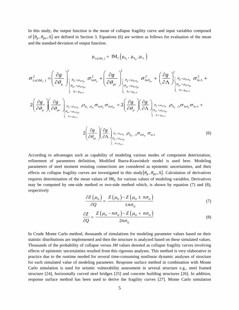
In this study, the output function is the mean of collapse fragility curve and input variables composed

of {𝜃𝑝 , 𝜃𝑝𝑐 , Λ} are defined in Section 3. Equations (6) are written as follows for evaluation of the mean

and the standard deviation of output function.

p pcC

C θ θ Λ Ln IMμ IM μ , μ ,μ

lnln ln

lnln ln

ln Λln Λ ln Λ

2 22

2 2 2 2

ln ln lnΛ

μ μ μ

Λ

p pp pp pcC p p

pc pcpc pcpc pc

Ln IM

p pc

g g g

lnln

lnln

ln Λln Λ

, ln ln ,Λ ln lnΛ

μ μ

2 2Λ

p pp p pc p pc p pp

pc pcpc pc

p pc p

g g g g

ln

ln

ln Λ

,Λ ln lnΛ

μ

2 Λ

p ppc pc

pc pcpc

g g

(6)

According to advantages such as capability of modeling various modes of component deterioration,

refinement of parameters definition, Modified Ibarra-Krawinkelr model is used here. Modeling

parameters of steel moment resisting connections are considered as epistemic uncertainties, and their

effects on collapse fragility curves are investigated in this study{𝜃𝑝 , 𝜃𝑝𝑐 , Λ}. Calculation of derivatives

requires determination of the mean values of IMC for various values of modeling variables. Derivatives

may be computed by one-side method or two-side method which, is shown by equation (7) and (8),

respectively

Q Q Q Q

Q

Z Z Z n

Q n

(7)

2

Q Q Q Q

Q

Z n Z nZ

Q n

(8)

In Crude Monte Carlo method, thousands of simulations for modeling parameter values based on their

statistic distributions are implemented and then the structure is analyzed based on these simulated values.

Thousands of the probability of collapse versus IM values denoted as collapse fragility curves involving

effects of epistemic uncertainties resulted from this rigorous analyses. This method is very elaborative in

practice due to the runtime needed for several time-consuming nonlinear dynamic analyses of structure

for each simulated value of modeling parameter. Response surface method in combination with Monte

Carlo simulation is used for seismic vulnerability assessment in several structure e.g., steel framed

structure [24], horizontally curved steel bridges [25] and concrete building structures [26]. In addition,

response surface method has been used to derive the fragility curves [27]. Monte Carlo simulation

6

applying a predefined regressed function, as response surface, has been proposed as an alternative to

substitute time history dynamic analysis and to reduce the computational effort in the context of the

previous researches. In this method, first, fixed formats of functions were interpolated to the limited

number of simulations of modeling variables as inputs, which lead to resultant means and standard

deviations of collapse fragility curves and as outputs of the function. In the next step, means and standard

deviations of collapse fragility curves for a large number of simulations of modeling parameters are

calculated applying derived analytical functions. The cost of reducing analysis time in the response

surface–based method is loss of accuracy in approximated collapse fragility curves. To overcome this

deficiency and to reduce the simulation runtime, the Monte Carlo along with inference method such as

ANN and ANFIS Methods in lieu of Response Surface method may be suggested. In this paper, ANFIS

Method is used for prediction the mean and the standard deviation of fragility curves for the first time.

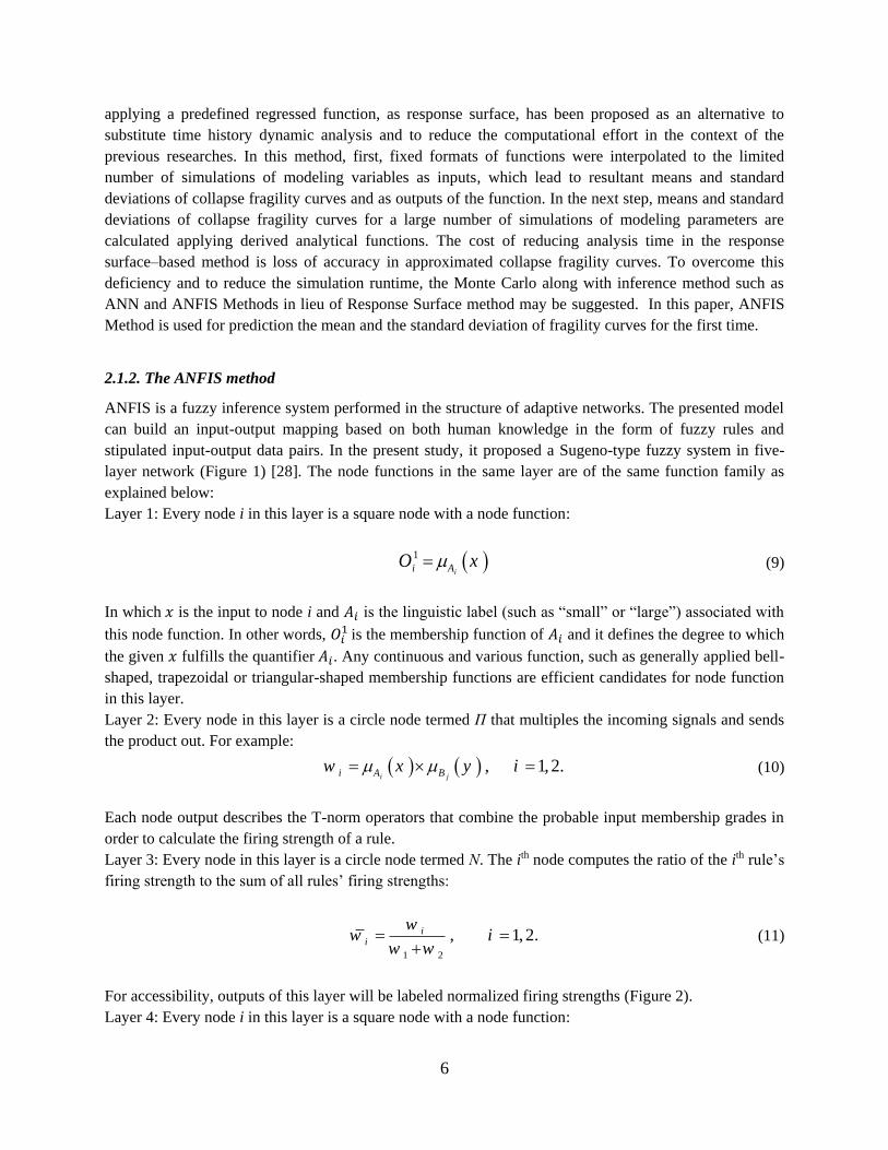
2.1.2. The ANFIS method

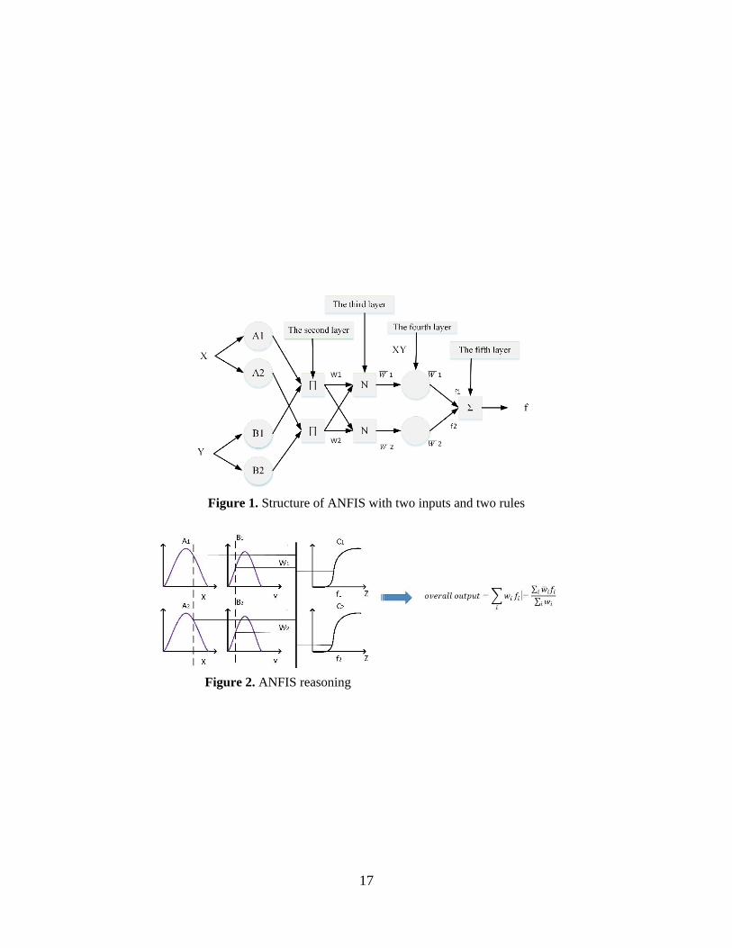
ANFIS is a fuzzy inference system performed in the structure of adaptive networks. The presented model

can build an input-output mapping based on both human knowledge in the form of fuzzy rules and

stipulated input-output data pairs. In the present study, it proposed a Sugeno-type fuzzy system in five-

layer network (Figure 1) [28]. The node functions in the same layer are of the same function family as

explained below:

Layer 1: Every node i in this layer is a square node with a node function:

1

ii AO x (9)

In which 𝑥 is the input to node i and 𝐴𝑖 is the linguistic label (such as “small” or “large”) associated with

this node function. In other words, 𝑂𝑖1 is the membership function of 𝐴𝑖 and it defines the degree to which

the given 𝑥 fulfills the quantifier 𝐴𝑖. Any continuous and various function, such as generally applied bell-

shaped, trapezoidal or triangular-shaped membership functions are efficient candidates for node function

in this layer.

Layer 2: Every node in this layer is a circle node termed Π that multiples the incoming signals and sends

the product out. For example:

, 1,2.i ji A Bw x y i (10)

Each node output describes the T-norm operators that combine the probable input membership grades in

order to calculate the firing strength of a rule.

Layer 3: Every node in this layer is a circle node termed Ν. The ith node computes the ratio of the ith rule’s

firing strength to the sum of all rules’ firing strengths:

1 2

, 1, 2.ii

ww i

w w

(11)

For accessibility, outputs of this layer will be labeled normalized firing strengths (Figure 2).

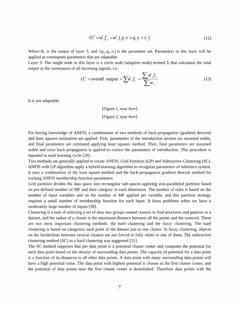
Layer 4: Every node i in this layer is a square node with a node function:

7

4

i i i i i i iO w f w p x q y r (12)

Where �̅�𝑖 is the output of layer 3, and {𝑝𝑖 , 𝑞𝑖 , 𝑟𝑖} is the parameter set. Parameters in this layer will be

applied as consequent parameters that are adaptable.

Layer 5: The single node in this layer is a circle node (adaptive node) termed Σ that calculates the total

output as the summation of all incoming signals, i.e.

5

i iii i i

i ii

w fO overall output w f

w

(13)

It is not adaptable.

[Figure 1, near here]


For having knowledge of ANFIS, a combination of two methods of back-propagation (gradient descent)

and least squares estimation are applied. First, parameters of the introduction section are assumed stable,

and final parameters are estimated applying least squares method. Then, final parameters are assumed

stable and error back-propagation is applied to correct the parameters of introduction. This procedure is

repeated in each learning cycle [29].

Two methods are generally applied to create ANFIS: Grid Partition (GP) and Subtractive Clustering (SC).

ANFIS with GP algorithm apply a hybrid-learning algorithm to recognize parameters of inference system.

It uses a combination of the least square method and the back-propagation gradient descent method for

training ANFIS membership function parameters.

Grid partition divides the data space into rectangular sub-spaces applying axis-paralleled partition based

on pre-defined number of MF and their category in each dimension. The number of rules is based on the

number of input variables and on the number of MF applied per variable, and this partition strategy

requires a small number of membership function for each input. It faces problems when we have a

moderately large number of inputs [30].

Clustering is a task of selecting a set of data into groups named clusters to find structures and patterns in a

dataset, and the radius of a cluster is the maximum distance between all the points and the centroid. There

are two most important clustering methods: the hard clustering and the fuzzy clustering. The hard

clustering is based on categorize each point of the dataset just to one cluster. In fuzzy clustering, objects

on the borderlines between several clusters are not forced to fully relate to one of them. The subtractive

clustering method (SC) as a hard clustering was suggested [31].

The SC method supposes that per data point is a potential cluster center and computes the potential for

each data point based on the density of surrounding data points. The capacity of potential for a data point

is a function of its distances to all other data points. A data point with many surrounding data points will

have a high potential value. The data point with highest potential is chosen as the first cluster center, and

the potential of data points near the first cluster center is demolished. Therefore data points with the

8

highest remaining potential as the next cluster center and the potential of data points near the new cluster

center are demolished.

It is remarkable that the important radius of cluster is vital for deciding the number of clusters and data

points outside this radius has little effect on the potential decision. Also, a smaller radius results in many

smaller clusters in the data space, which leads to more rules [31].

In this study, GP, SC, and another technique which is named Fuzzy C-means (FCM) are applied to

generate the ANFIS model. FCM is a strong unsupervised algorithm. FCM clustering was first informed

by Dunn [32]. It was extended by Bezdek (1981). FCM is an algorithm where per data point has a

membership degree between 0 and 1 to each fuzzy subset. In other words, each data in FCM can be

related to all groups with various membership grades. The algorithm generates an optimal c partition by

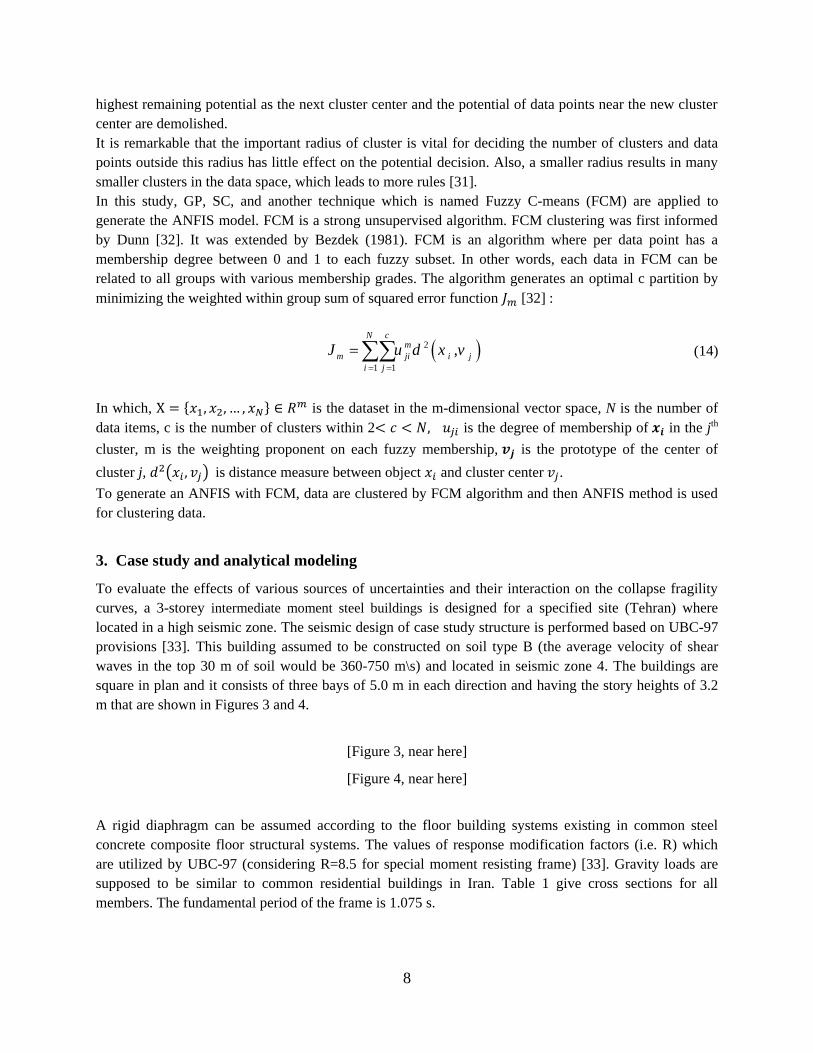
minimizing the weighted within group sum of squared error function 𝐽𝑚 [32] :

2

1 1

, N c

m

m ji i j

i j

J u d x v

(14)

In which, Χ = {𝑥1, 𝑥2, … , 𝑥𝑁} ∈ 𝑅𝑚 is the dataset in the m-dimensional vector space, N is the number of

data items, c is the number of clusters within 2< 𝑐 < 𝑁, 𝑢𝑗𝑖 is the degree of membership of 𝒙𝒊 in the jth

cluster, m is the weighting proponent on each fuzzy membership, 𝒗𝒋 is the prototype of the center of

cluster j, 𝑑2(𝑥𝑖 , 𝑣𝑗) is distance measure between object 𝑥𝑖 and cluster center 𝑣𝑗.

To generate an ANFIS with FCM, data are clustered by FCM algorithm and then ANFIS method is used

for clustering data.

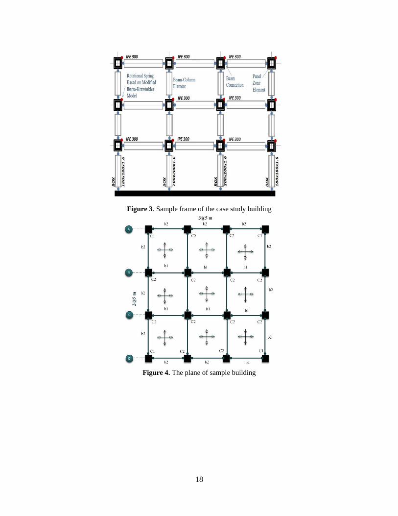
3. Case study and analytical modeling

To evaluate the effects of various sources of uncertainties and their interaction on the collapse fragility

curves, a 3-storey intermediate moment steel buildings is designed for a specified site (Tehran) where

located in a high seismic zone. The seismic design of case study structure is performed based on UBC-97

provisions [33]. This building assumed to be constructed on soil type B (the average velocity of shear

waves in the top 30 m of soil would be 360-750 m\s) and located in seismic zone 4. The buildings are

square in plan and it consists of three bays of 5.0 m in each direction and having the story heights of 3.2

m that are shown in Figures 3 and 4.



A rigid diaphragm can be assumed according to the floor building systems existing in common steel

concrete composite floor structural systems. The values of response modification factors (i.e. R) which

are utilized by UBC-97 (considering R=8.5 for special moment resisting frame) [33]. Gravity loads are

supposed to be similar to common residential buildings in Iran. Table 1 give cross sections for all

members. The fundamental period of the frame is 1.075 s.

9

[Table 1, near here]

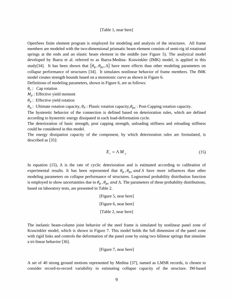
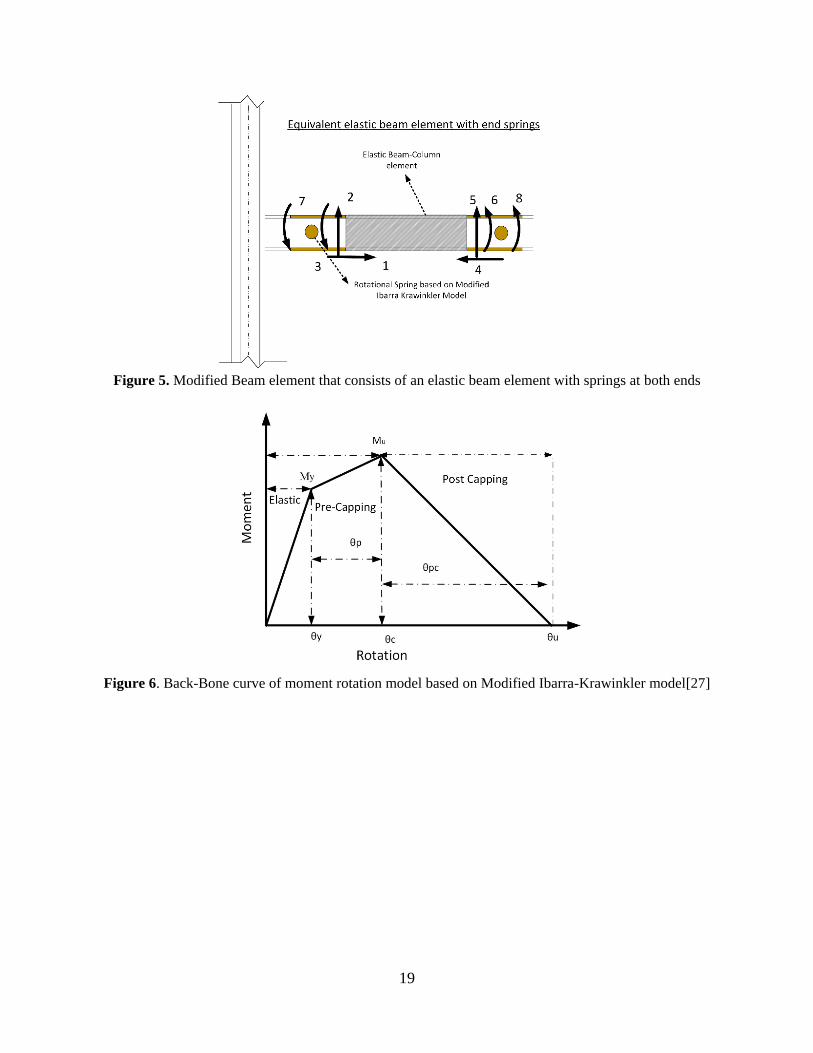
OpenSees finite element program is employed for modeling and analysis of the structures. All frame

members are modeled with the two-dimensional prismatic beam element consists of semi-rig id rotational

springs at the ends and an elastic beam element in the middle (see Figure 5). The analytical model

developed by Ibarra et al. referred to as Ibarra-Medina- Krawinkler (IMK) model, is applied in this

study[34]. It has been shown that {𝜃𝑝 , 𝜃𝑝𝑐 , Λ} have more effects than other modeling parameters on

collapse performance of structures [34]. It simulates nonlinear behavior of frame members. The IMK

model creates strength bounds based on a monotonic curve as shown in Figure 6.

Definitions of modeling parameters, shown in Figure 6, are as follows:

𝜃𝑐 : Cap rotation

𝑀𝑦 : Effective yield moment

𝜃𝑦 : Effective yield rotation

𝜃𝑢 : Ultimate rotation capacity, 𝜃𝑃 : Plastic rotation capacity,𝜃𝑝𝑐 : Post-Capping rotation capacity.

The hysteretic behavior of the connection is defined based on deterioration rules, which are defined

according to hysteretic energy dissipated in each load-deformation cycle.

The deterioration of basic strength, post capping strength, unloading stiffness and reloading stiffness

could be considered in this model.

The energy dissipation capacity of the component, by which deterioration rules are formulated, is

described as [35]:

Λ t yE M (15)

In equation (15), Λ is the rate of cyclic deterioration and is estimated according to calibration of

experimental results. It has been represented that 𝜃𝑝 , 𝜃𝑝𝑐 𝑎𝑛𝑑 Λ have more influences than other

modeling parameters on collapse performance of structures. Lognormal probability distribution function

is employed to show uncertainties due to 𝜃𝑝 , 𝜃𝑝𝑐 𝑎𝑛𝑑 Λ. The parameters of these probability distributions,

based on laboratory tests, are presented in Table 2.




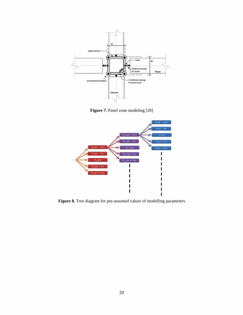
The inelastic beam-column joint behavior of the steel frame is simulated by nonlinear panel zone of

Krawinkler model, which is shown in Figure 7. This model holds the full dimension of the panel zone

with rigid links and controls the deformation of the panel zone by using two bilinear springs that simulate

a tri-linear behavior [36].


A set of 40 strong ground motions represented by Medina [37], named as LMSR records, is chosen to

consider record-to-record variability in estimating collapse capacity of the structure. IM-based

10

formulation is used to derive collapse fragility curves from performing IDA of the sample structure.

These records are normal strong ground motions recorded in California region and do not involve pulse –

type near-field features that is introduced in Table 3. The hunt&fill tracing algorithm is used to scale

records in IDA method to achieve good performance [16].

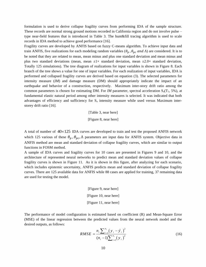
Fragility curves are developed by ANFIS based on fuzzy C-means algorithm. To achieve input data and

train ANFIS, five realizations for each modeling random variables (𝜃𝑝 , 𝜃𝑝𝑐 𝑎𝑛𝑑 Λ) are considered. It is to

be noted that they are related to mean, mean minus and plus one standard deviation and mean minus and

plus two standard deviations (mean, mean ±1× standard deviation, mean ±2.0× standard deviation,

Totally 125 simulations). The tree diagram of realizations for input variables is shown in Figure 8. Each

branch of the tree shows a value for one of input variables. For each realization of input variables, IDA is

performed and collapsed fragility curves are derived based on equation (3). The selected parameters for

intensity measure (IM) and damage measure (DM) should appropriately indicate the impact of an

earthquake and behavior of a construction, respectively. Maximum inter-story drift ratio among the

common parameters is chosen for estimating DM. For IM parameter, spectral acceleration Sa(T1, 5%), at

fundamental elastic natural period among other intensity measures is selected. It was indicated that both

advantages of efficiency and sufficiency for Sa intensity measure while used versus Maximum inter-

storey drift ratio [16].



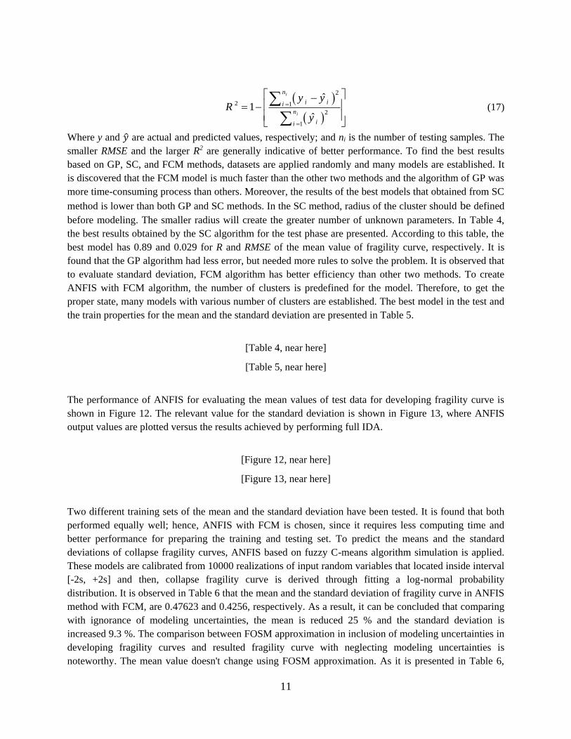
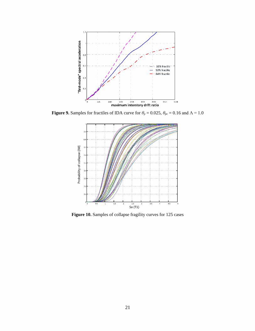
A total of number of 40 125 IDA curves are developed to train and test the proposed ANFIS network

which 125 various of these 𝜃𝑝 , 𝜃𝑝𝑐 , Λ parameters are input data for ANFIS system. Objective data in

ANFIS method are mean and standard deviation of collapse fragility curves, which are similar to output

functions in FOSM method.

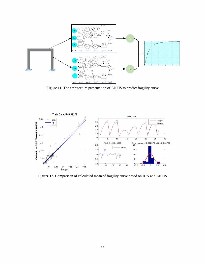
A sample of IDA curves and fragility curves for 10 cases are presented in Figures 9 and 10, and the

architecture of represented neural networks to predict mean and standard deviation values of collapse

fragility curves is shown in Figure 11. As it is shown in this figure, after analyzing for each scenario,

which includes epistemic uncertainty, ANFIS predicts mean and standard deviation of collapse fragility

curves. There are 125 available data for ANFIS while 88 cases are applied for training, 37 remaining data

are used for testing the model.




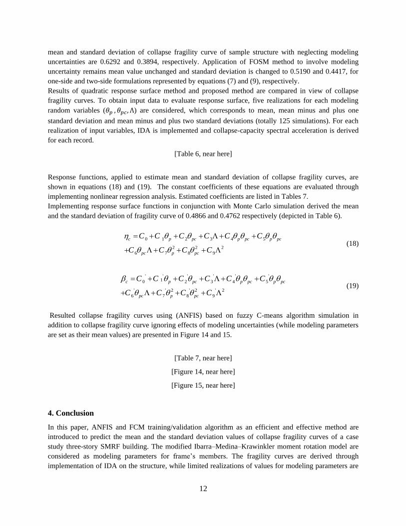
The performance of model configuration is estimated based on coefficient (R) and Mean-Square Error

(MSE) of the linear regression between the predicted values from the neural network model and the

desired outputs, as follows:

2

1

2

1( 1

ˆ

)

i

i

n

i i ii

n

i ii

n y yRMSE

n y

(16)

11

2

2 1

2

1

ˆ

ˆ1

i

i

n

i ii

n

ii

y yR

y

(17)

Where y and �̂� are actual and predicted values, respectively; and ni is the number of testing samples. The

smaller RMSE and the larger R2 are generally indicative of better performance. To find the best results

based on GP, SC, and FCM methods, datasets are applied randomly and many models are established. It

is discovered that the FCM model is much faster than the other two methods and the algorithm of GP was

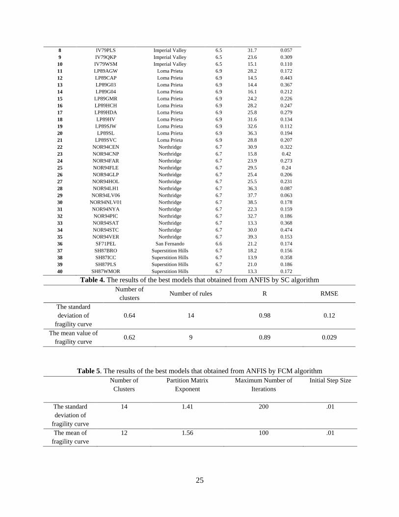
more time-consuming process than others. Moreover, the results of the best models that obtained from SC

method is lower than both GP and SC methods. In the SC method, radius of the cluster should be defined

before modeling. The smaller radius will create the greater number of unknown parameters. In Table 4,

the best results obtained by the SC algorithm for the test phase are presented. According to this table, the

best model has 0.89 and 0.029 for R and RMSE of the mean value of fragility curve, respectively. It is

found that the GP algorithm had less error, but needed more rules to solve the problem. It is observed that

to evaluate standard deviation, FCM algorithm has better efficiency than other two methods. To create

ANFIS with FCM algorithm, the number of clusters is predefined for the model. Therefore, to get the

proper state, many models with various number of clusters are established. The best model in the test and

the train properties for the mean and the standard deviation are presented in Table 5.



The performance of ANFIS for evaluating the mean values of test data for developing fragility curve is

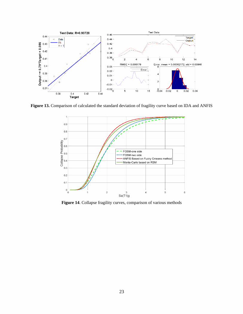
shown in Figure 12. The relevant value for the standard deviation is shown in Figure 13, where ANFIS

output values are plotted versus the results achieved by performing full IDA.



Two different training sets of the mean and the standard deviation have been tested. It is found that both

performed equally well; hence, ANFIS with FCM is chosen, since it requires less computing time and

better performance for preparing the training and testing set. To predict the means and the standard

deviations of collapse fragility curves, ANFIS based on fuzzy C-means algorithm simulation is applied.

These models are calibrated from 10000 realizations of input random variables that located inside interval

[-2s, +2s] and then, collapse fragility curve is derived through fitting a log-normal probability

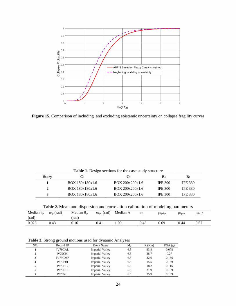
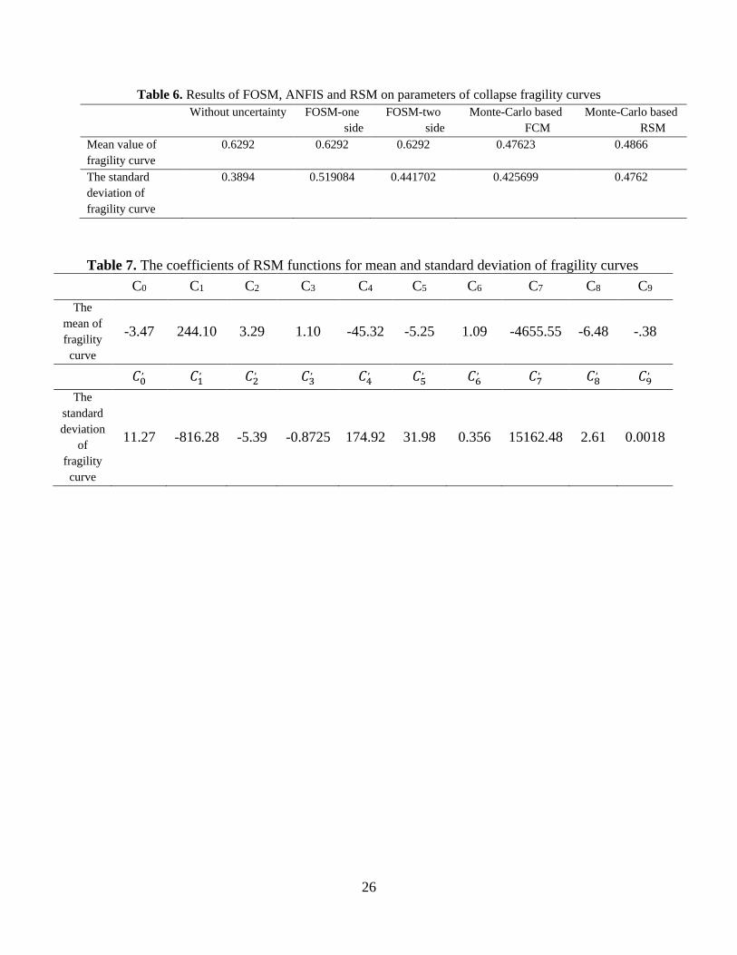
distribution. It is observed in Table 6 that the mean and the standard deviation of fragility curve in ANFIS

method with FCM, are 0.47623 and 0.4256, respectively. As a result, it can be concluded that comparing

with ignorance of modeling uncertainties, the mean is reduced 25 % and the standard deviation is

increased 9.3 %. The comparison between FOSM approximation in inclusion of modeling uncertainties in

developing fragility curves and resulted fragility curve with neglecting modeling uncertainties is

noteworthy. The mean value doesn't change using FOSM approximation. As it is presented in Table 6,

12

mean and standard deviation of collapse fragility curve of sample structure with neglecting modeling

uncertainties are 0.6292 and 0.3894, respectively. Application of FOSM method to involve modeling

uncertainty remains mean value unchanged and standard deviation is changed to 0.5190 and 0.4417, for

one-side and two-side formulations represented by equations (7) and (9), respectively.

Results of quadratic response surface method and proposed method are compared in view of collapse

fragility curves. To obtain input data to evaluate response surface, five realizations for each modeling

random variables (𝜃𝑝 , 𝜃𝑝𝑐 , Λ) are considered, which corresponds to mean, mean minus and plus one

standard deviation and mean minus and plus two standard deviations (totally 125 simulations). For each

realization of input variables, IDA is implemented and collapse-capacity spectral acceleration is derived

for each record.


Response functions, applied to estimate mean and standard deviation of collapse fragility curves, are

shown in equations (18) and (19). The constant coefficients of these equations are evaluated through

implementing nonlinear regression analysis. Estimated coefficients are listed in Tables 7.

Implementing response surface functions in conjunction with Monte Carlo simulation derived the mean

and the standard deviation of fragility curve of 0.4866 and 0.4762 respectively (depicted in Table 6).

0 1 2 3 4 5

2 2 2

6 7 8 9

c p pc p pc p pc

pc p pc

C C C C C C

C C C C

(18)

' ' ' ' ' '10 2 3 4 5

' ' 2 ' 2 ' 2

6 7 8 9

c p pc p pc p pc

pc p pc

C C C C C C

C C C C

(19)

Resulted collapse fragility curves using (ANFIS) based on fuzzy C-means algorithm simulation in

addition to collapse fragility curve ignoring effects of modeling uncertainties (while modeling parameters

are set as their mean values) are presented in Figure 14 and 15.




4. Conclusion

In this paper, ANFIS and FCM training/validation algorithm as an efficient and effective method are

introduced to predict the mean and the standard deviation values of collapse fragility curves of a case

study three-story SMRF building. The modified Ibarra–Medina–Krawinkler moment rotation model are

considered as modeling parameters for frame’s members. The fragility curves are derived through

implementation of IDA on the structure, while limited realizations of values for modeling parameters are

13

presumed. To this end, three inputs (θP, θpc and Λ) and two output data values (mean and standard

deviation) are considered. The system is trained by a dataset of 125 values obtained from 5000 IDA

curves. Then, dataset consisting of 10000 inputs are applied to predict a basis fragility curve with aleatory

and epistemic uncertainty. As a result, involvement of modeling uncertainties reduces the mean and

increases the standard deviation of obtained fragility curves. To compare the results, collapse fragility

curves of sample frame are derived using other approaches such as FOSM and RSM methods. Modeling

parameters involved in moment-rotation relationship of connections, entitled (θp, θpc and Λ) are

considered as epistemic uncertain parameters. The effects of epistemic uncertainties, on collapse fragility

curves, are estimated by aforementioned methods. Many ANFIS models based on GP, SC, and FCM are

expanded, and it is understood that the ANFIS-FCM predicts the fragility curve with higher accuracy than

other methods (GP, SC). GP is more time-consuming process than other methods and needs more rules to

solve the problem and in the SC method, the problem is radius value of the cluster, which should be

defined before modeling, hence the smaller radius will create the greater number of unknown parameters.

In this respect, FCM algorithm has better efficiency than other two methods. Therefore, FCM algorithm

in comparison with Monte Carlo method are known as precise methodology. Nevertheless, the proposed

method presented here demonstrates a small prediction error and leads to comparable results with those

obtained using Monte Carlo method.

5. References

1. Whittaker, A., Hamburger, R. and Mahoney, M. "Performance-based engineering of

buildings and infrastructure for extreme loadings", in Proceedings, AISC-SINY Symposium

on Resisting Blast and Progressive Collapse. American Institute of Steel Construction, New

York (2003).

2. Khurana, A. "Report on earthquake of 8th October in some parts of northern India" ( 2005).

3. Liel, A.B., Haselton, C.B., Deierlein, G.G. and Baker, J.W. "Incorporating modeling

uncertainties in the assessment of seismic collapse risk of buildings", Structural Safety, 31,

pp. 197-211 (2009).

4. Ibarra L.F. and Krawinkler, H. "Global collapse of frame structures under seismic

excitations", Pacific Earthquake Engineering Research Center (2005).

5. Benjamin, J.R. and Cornell, C.A. "Probability, statistics, and decision for civil engineers",

Courier Corporation (2014).

6. Zareian, F., Krawinkler, H., Ibarra, L. and Lignos, D. "Basic concepts and performance

measures in prediction of collapse of buildings under earthquake ground motions," The

Structural Design of Tall and Special Buildings, 19, pp. 167-181 (2010).

7. Khojastehfar, E., Beheshti-Aval, S.B., Zolfaghari, M.R. and Nasrollahzade, K. "Collapse

fragility curve development using Monte Carlo simulation and artificial neural network",

Proceedings of the Institution of Mechanical Engineers, Part O: Journal of Risk and

Reliability, 228, pp. 301-312 (2014).

8. Beheshti-Aval, S.B., Khojastehfar, E., Noori, M. and Zolfaghar, M.R. " A comprehensive

collapse fragility assessment of moment resisting steel frames considering various sources of

uncertainties", Canadian Journal of Civil Engineering, vol. 43(2): 118-131 (2016).

9. Lagaros N.D. and Fragiadakis, M. "Fragility assessment of steel frames using neural

networks", Earthquake Spectra, 23, pp. 735-752 (2007).

14

10. Mitropoulou C.C. and Papadrakakis, M. "Developing fragility curves based on neural

network IDA predictions", Engineering Structures, 33, pp. 3409-3421 (2011).

11. Cardaliaguet, P. and Euvrard, G. "Approximation of a function and its derivative with a

neural network", Neural Networks, 5, pp. 207-220 (1992).

12. Li, X. "Simultaneous approximations of multivariate functions and their derivatives by

neural networks with one hidden layer", Neurocomputing, 12, pp. 327-343 (1996).

13. Chapman, O. and Crossland, A. "Neural networks in probabilistic structural mechanics", in

Probabilistic Structural Mechanics Handbook, pp. 317-330 (1995).

14. Atmaca, H., Cetişli, B. and Yavuz, H.S. "The Comparison of Fuzzy Inference Systems and

Neural Network Approaches with ANFIS Method for Fuel Consumption Data", Yavuz

Osmangazi University, Electrical and Electronic Engineering Department (2001).

15. Farahani, M. K. and Mehralian, S. "Comparison Between Artificial Neural Network and

Neuro-Fuzzy for Gold Price Prediction", Fuzzy Systems (IFSC), 13th Iranian

Conference on, At Qazvin, Iran (2013).

16. Vamvatsikos D. and Cornell, C.A. "Incremental dynamic analysis", Earthquake Engineering

& Structural Dynamics, 31, pp. 491-514 (2002).

17. Zareian, F., Lignos, D.G. and Krawinkler, H. "Quantification of modeling uncertainties for

collapse assessment of structural systems under seismic excitations," in Proceedings of the

2nd international conference on computational methods in structural dynamics and

earthquake engineering (COMPDYN 2009), pp. 22-24 (2009).

18. Beheshti-Aval, S.B., Verki A.M. and Rastegaran, M. " Systematical Approach to Evaluate

Probability of Steel MRF Buildings Based on Engineering Demand and Intensity Measure",

Proc. of the Intl. Conf. on Advances in Civil, Structural and Mechanical Engineering (2014).

19. Zareian F. and Krawinkler, H. "Assessment of probability of collapse and design for

collapse safety", Earthquake Engineering & Structural Dynamics, vol. 36, pp. 1901-1914,

(2007).

20. Celarec D. and Dolšek, M. "The impact of modelling uncertainties on the seismic

performance assessment of reinforced concrete frame buildings", Engineering Structures,

52, pp. 340-354 (2013).

21. Rubinstein R.Y. and Kroese, D.P. "Simulation and the Monte Carlo method", vol. 707: John

Wiley & Sons (2011).

22. Esteva, L. and Ruiz, S. E. "Seismic failure rates of multistory frames", Journal of Structural

Engineering, 115, pp. 268-284 (1989).

23. Baker J.W. and Cornell, C.A. "A vector‐valued ground motion intensity measure consisting

of spectral acceleration and epsilon", Earthquake Engineering & Structural Dynamics, 34,

pp. 1193-1217 (2005).

24. He, J.N. and Wang, Z. "Analysis on System Reliability of Steel Framework Structure and

Optimal Design , Applied Mechanics and Materials, 105,pp. 902-906 (2011).

25. Seo, J. and Linzell, D.G. "Horizontally curved steel bridge seismic vulnerability assessment

", Engineering Structures, 34: 21-32 (2012).

26. Liel, A.B., Haselton, C.B., Deierlein, G.G. and Baker, J.W. "Incorporating modelling

uncertainties in the assessment of seismic collapse risk of buildings", Structural Safety,

31(2), pp. 197-211 (2009).

27. Rajeev, P. and Tesfamariam, S. "Seismic fragilities for reinforced concrete buildings with

consideration of irregularities", Structural Safety, 39,pp. 1-13 (2012).

15

28. Jang, J.S.R. "ANFIS: adaptive-network-based fuzzy inference system", Systems, Man and

Cybernetics, IEEE Transactions on, 23, pp. 665-685 (1993).

29. Bezdek, J.C. "Pattern recognition with fuzzy objective function algorithms", Springer

Science & Business Media (2013).

30. Jang, J.S.R., Sun, C.T. and Mizutani, E. "Neuro-fuzzy and soft computing; a computational

approach to learning and machine intelligence", (1997).

31. Chiu, S.L. "Fuzzy model identification based on cluster estimation", Journal of intelligent

and Fuzzy systems, 2, pp. 267-278 (1994).

32. Dunn, J.C. "A fuzzy relative of the ISODATA process and its use in detecting compact

well-separated clusters", (1973).

33. UBC, U.B.C. "Uniform building code," in Int. Conf. Building Officials" (1997).

34. Ellingwood B.R. and Kinali, K. "Quantifying and communicating uncertainty in seismic risk

assessment," Structural Safety, 31, pp. 179-187 (2009).

35. Ibarra, L.F., Medina, R.A. and Krawinkler, H. "Hysteretic models that incorporate strength

and stiffness deterioration", Earthquake engineering and structural dynamics, 34, pp. 1489-

1512 (2005).

36. Foutch D. A. and Yun, S.Y. "Modeling of steel moment frames for seismic loads", Journal

of Constructional Steel Research, 58, pp. 529-564 (2002).

37. Medina R.A. and Krawinkler, H. "Seismic demands for nondeteriorating frame structures

and their dependence on ground motions", Pacific Earthquake Engineering Research Center

(2004).

Biographies

Fooad Karimi Ghaleh Jough was born in 1982. He obtained his BS degree in Civil Engineering from

Tabriz Azad University, Iran in 2006, and MSc degree in Structural Engineering from Sistan &

Baluchestan University, Zahedan, Iran in 2008. He received his PhD in earthquake engineering from

Eastern Mediterranean University, Famagusta, Turkey in 2016 and has been a faculty member at Sarab

branch of Islamic Azad University. His research interests include vulnerability assessment of existing

buildings and using metaheuristic algorithms in seismic risk analysis.

Seyed Bahram Beheshti Aval is associate professor at Civil Engineering Department at the K.N. Toosi

University of Technology. He received his PhD degree from the Sharif University of Technology (SUT)

in 1999. He is responsible for teaching of courses in design of reinforced concrete structures, energy

methods in finite element analysis, seismic rehabilitation of existing buildings, structural reliability, and

probabilistic seismic analysis of structures. His research activities have included studies of seismic

reliability analysis of structures, composite structures, and various problems in seismic design of

structures. He has authored more than 50 published papers and two textbooks entitled Energy Principles

and Variational Methods in Finite Element Analysis and Seismic Rehabilitation of Existing Buildings.

https://blume.stanford.edu/rms-tech/probabilistic-seismic-demand-analysis-nonlinear-structures

16

The list of figures’ captions

Figure 1. Structure of ANFIS with two inputs and two rules

Figure 2. ANFIS reasoning

Figure 3. Sample frame of the case study building

Figure 4. The plane of sample building

Figure 5. Modified Beam element that consists of an elastic beam element with springs at both ends

Figure 6. Back-Bone curve of moment rotation model based on Modified Ibarra-Krawinkler model[27]

Figure 7. Panel zone modeling [28]

Figure 8. Tree diagram for pre-assumed values of modelling parameters

Figure 9. Samples for fractiles of IDA curve for θp = 0.025, θpc = 0.16 and Λ = 1.0

Figure 10. Samples of collapse fragility curves for 125 cases

Figure 11. The architecture presentation of ANFIS to predict fragility curve

Figure 12. Comparison of calculated mean of fragility curve based on IDA and ANFIS

Figure 13. Comparison of calculated the standard deviation of fragility curve based on IDA and ANFIS

Figure 14. Collapse fragility curves, comparison of various methods

Figure 15. Comparison of including and excluding epistemic uncertainty on collapse fragility curves

The list of tables’ captions

Table 1. Design sections for the case study structure

Table 2. Mean and dispersion and correlation calibration of modeling parameters

Table 3. Strong ground motion used for dynamic Analysis

Table 4. The results of the best models that obtained from ANFIS by SC algorithm

Table 5. The results of the best models that obtained from ANFIS by FCM algorithm.

Table 6. Results of FOSM, ANFIS and RSM on parameters of collapse fragility curves

Table 7. The coefficients of RSM functions for mean and standard deviation of fragility curves

17

Figure 1. Structure of ANFIS with two inputs and two rules

Figure 2. ANFIS reasoning

18

Figure 3. Sample frame of the case study building

Figure 4. The plane of sample building

19

Figure 5. Modified Beam element that consists of an elastic beam element with springs at both ends

Figure 6. Back-Bone curve of moment rotation model based on Modified Ibarra-Krawinkler model[27]

20

Figure 7. Panel zone modeling [28]

Figure 8. Tree diagram for pre-assumed values of modelling parameters

21

Figure 9. Samples for fractiles of IDA curve for θp = 0.025, θpc = 0.16 and Λ = 1.0

Figure 10. Samples of collapse fragility curves for 125 cases

22

Figure 11. The architecture presentation of ANFIS to predict fragility curve

Figure 12. Comparison of calculated mean of fragility curve based on IDA and ANFIS

23

Figure 13. Comparison of calculated the standard deviation of fragility curve based on IDA and ANFIS

Figure 14. Collapse fragility curves, comparison of various methods

24

Figure 15. Comparison of including and excluding epistemic uncertainty on collapse fragility curves

Table 1. Design sections for the case study structure

Story C1 C2 B1 B2

1 BOX 180x180x1.6 BOX 200x200x1.6 IPE 300 IPE 330



Table 2. Mean and dispersion and correlation calibration of modeling parameters

Median θp

(rad)

σθp (rad) Median θpc

(rad)

σθpc (rad) Median Λ σΛ ρθp,θpc ρθp,Λ ρθpc,Λ

0.025 0.43 0.16 0.41 1.00 0.43 0.69 0.44 0.67

Table 3. Strong ground motions used for dynamic Analyses NO. Record ID Event Name Mw R (Km) PGA (g)

1 IV79CAL Imperial Valley 6.5 23.8 0.078

2 IV79CHI Imperial Valley 6.5 28.7 0.27

3 IV79CMP Imperial Valley 6.5 32.6 0.186

4 IV79E01 Imperial Valley 6.5 15.5 0.139



7 IV79NIL Imperial Valley 6.5 35.9 0.109

25

8 IV79PLS Imperial Valley 6.5 31.7 0.057

9 IV79QKP Imperial Valley 6.5 23.6 0.309

10 IV79WSM Imperial Valley 6.5 15.1 0.110

11 LP89AGW Loma Prieta 6.9 28.2 0.172

12 LP89CAP Loma Prieta 6.9 14.5 0.443

13 LP89G03 Loma Prieta 6.9 14.4 0.367

14 LP89G04 Loma Prieta 6.9 16.1 0.212

15 LP89GMR Loma Prieta 6.9 24.2 0.226

16 LP89HCH Loma Prieta 6.9 28.2 0.247

17 LP89HDA Loma Prieta 6.9 25.8 0.279

18 LP89HV Loma Prieta 6.9 31.6 0.134

19 LP89SJW Loma Prieta 6.9 32.6 0.112

20 LP89SL Loma Prieta 6.9 36.3 0.194

21 LP89SVC Loma Prieta 6.9 28.8 0.207

22 NOR94CEN Northridge 6.7 30.9 0.322

23 NOR94CNP Northridge 6.7 15.8 0.42

24 NOR94FAR Northridge 6.7 23.9 0.273

25 NOR94FLE Northridge 6.7 29.5 0.24

26 NOR94GLP Northridge 6.7 25.4 0.206

27 NOR94HOL Northridge 6.7 25.5 0.231

28 NOR94LH1 Northridge 6.7 36.3 0.087

29 NOR94LV06 Northridge 6.7 37.7 0.063

30 NOR94NLV01 Northridge 6.7 38.5 0.178

31 NOR94NYA Northridge 6.7 22.3 0.159

32 NOR94PIC Northridge 6.7 32.7 0.186

33 NOR94SAT Northridge 6.7 13.3 0.368

34 NOR94STC Northridge 6.7 30.0 0.474

35 NOR94VER Northridge 6.7 39.3 0.153

36 SF71PEL San Fernando 6.6 21.2 0.174

37 SH87BRO Superstition Hills 6.7 18.2 0.156

38 SH87ICC Superstition Hills 6.7 13.9 0.358

39 SH87PLS Superstition Hills 6.7 21.0 0.186

40 SH87WMOR Superstition Hills 6.7 13.3 0.172

Table 4. The results of the best models that obtained from ANFIS by SC algorithm

Number of

clusters Number of rules R RMSE

The standard

deviation of

fragility curve

0.64 14 0.98 0.12

The mean value of

fragility curve 0.62 9 0.89 0.029

Table 5. The results of the best models that obtained from ANFIS by FCM algorithm

Number of

Clusters

Partition Matrix

Exponent

Maximum Number of

Iterations

Initial Step Size

The standard

deviation of

fragility curve

14 1.41 200 .01

The mean of

fragility curve

12 1.56 100 .01

26

Table 6. Results of FOSM, ANFIS and RSM on parameters of collapse fragility curves

Without uncertainty FOSM-one

side

FOSM-two

side

Monte-Carlo based

FCM

Monte-Carlo based

RSM

Mean value of

fragility curve

0.6292 0.6292 0.6292 0.47623 0.4866

The standard

deviation of

fragility curve

0.3894 0.519084 0.441702 0.425699 0.4762

Table 7. The coefficients of RSM functions for mean and standard deviation of fragility curves

C0 C1 C2 C3 C4 C5 C6 C7 C8 C9

The

mean of

fragility

curve

-3.47 244.10 3.29 1.10 -45.32 -5.25 1.09 -4655.55 -6.48 -.38

𝐶0, 𝐶1

, 𝐶2

, 𝐶3

, 𝐶4

, 𝐶5

, 𝐶6

, 𝐶7

, 𝐶8

, 𝐶9

,

The

standard

deviation

of

fragility

curve

11.27 -816.28 -5.39 -0.8725 174.92 31.98 0.356 15162.48 2.61 0.0018

uncertainty analysis through development of seismic...

Documents