Uncertainty and Labor Contract Durations

Robert RichJoseph Tracy

December 8, 1999

Abstract

This paper provides an empirical investigation into the relationship between ex ante U.S.labor contract durations and uncertainty over the period 1970 to 1995. We construct measures ofinflation uncertainty as well as aggregate nominal and real uncertainty. The results not onlycorroborate previous findings of an inverse relationship between contract duration and inflationuncertainty, but also document that this relationship extends to both measures of aggregateuncertainty. We also explore the robustness of this relationship to the various measures ofinflation uncertainty that have appeared in the literature.

We thank Nathaniel Baum-Snow for his excellent research assistance. We received helpful commentsfrom seminar participants at the University of Missouri, New York University and Wharton. The viewsexpressed in this paper are those of the individual authors and do not necessarily reflect the position ofthe Federal Reserve Bank of New York or the Federal Reserve System. Address correspondence to theauthors at the Federal Reserve Bank of New York, Domestic Research Division, 33 Liberty Street, NewYork, NY 10045. Email: robert.rich@ny.frb.org or joseph.tracy@ny.frb.org

1The BLS defines a major union contract to be one which covers at least 1,000 workers. The exante duration as reported by the BLS is the number of months between the effective date of the contractand the planned expiration date. The ex post duration may differ from the ex ante durations due to earlyrenegotiations or delayed settlements (which effectively extend the duration of the contract). For theremainder of this paper, we will refer to the ex ante duration simply as the contract duration.

I. IntroductionIt is widely agreed that the existence of long-term labor contracts has potentially

important implications for the behavior of the macroeconomy. Specifically, contract length is

particularly important for issues relating to the efficacy of stabilization policies and the dynamic

behavior of aggregate fluctuations. For example, labor contracts, by limiting the actions of agents

during the duration of the contracts, can provide the monetary authority with an advantage in

reacting to shocks in an economy and a role for stabilizing output [Fischer (1977)]. In addition,

multi-period contracts can serve as a key propagation mechanism for shocks, with their structure

being central to the adjustment process of output, prices and wages. This latter consideration is

extremely relevant for the design and conduct of disinflation policy [Taylor (1980)].

Recent union labor contract renewals have resulted in significantly longer contracts being

signed than in the past. For example, the three major auto manufacturers and the United Auto

Workers signed four-year national contracts in their last round of negotiations, breaking a long

standing tradition of three-year contracts [Bloomberg (1999) and Hyde (1999)]. The United Steel

Workers and Kennecott Copper Corporation signed a five-year contract in October of 1996

[Thomson (1996)]. A six-year contract with Goodyear Tire Company was ratified by the United

Steel Workers in May of 1997 [Gamboa (1997)].

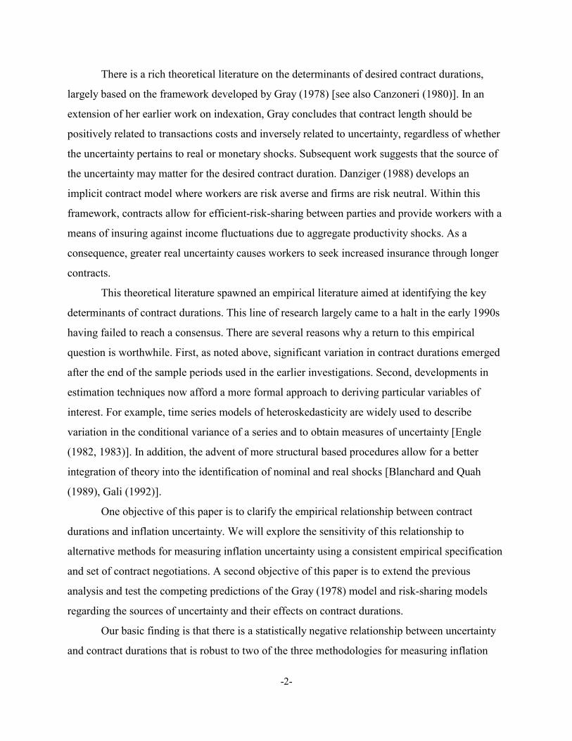
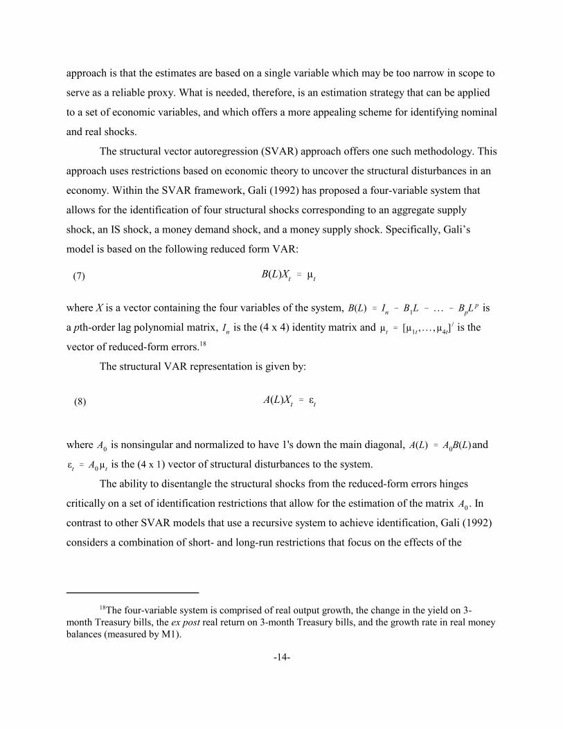
These examples illustrate an important recent trend in the duration of union labor

contracts. Figure 1 shows by year the 10th, 25th, 50th , 75th and 90th percentiles of the distribution

of ex ante contract duration for all major union contracts negotiated in that year and included in

the Bureau of Labor Statistics (BLS) data.1 Apart from some volatility in the early 1970s, the 10th

and 50th percentiles have been remarkably constant over this period. In contrast, the 90th

percentile shows a steady upward progression starting in the mid-1980s, with the 75th percentile

following suit beginning in the early 1990s. This recent shift in the distribution of contract

durations provides an important source of variation for identifying the underlying determinants of

the desired contract duration.

-2-

There is a rich theoretical literature on the determinants of desired contract durations,

largely based on the framework developed by Gray (1978) [see also Canzoneri (1980)]. In an

extension of her earlier work on indexation, Gray concludes that contract length should be

positively related to transactions costs and inversely related to uncertainty, regardless of whether

the uncertainty pertains to real or monetary shocks. Subsequent work suggests that the source of

the uncertainty may matter for the desired contract duration. Danziger (1988) develops an

implicit contract model where workers are risk averse and firms are risk neutral. Within this

framework, contracts allow for efficient-risk-sharing between parties and provide workers with a

means of insuring against income fluctuations due to aggregate productivity shocks. As a

consequence, greater real uncertainty causes workers to seek increased insurance through longer

contracts.

This theoretical literature spawned an empirical literature aimed at identifying the key

determinants of contract durations. This line of research largely came to a halt in the early 1990s

having failed to reach a consensus. There are several reasons why a return to this empirical

question is worthwhile. First, as noted above, significant variation in contract durations emerged

after the end of the sample periods used in the earlier investigations. Second, developments in

estimation techniques now afford a more formal approach to deriving particular variables of

interest. For example, time series models of heteroskedasticity are widely used to describe

variation in the conditional variance of a series and to obtain measures of uncertainty [Engle

(1982, 1983)]. In addition, the advent of more structural based procedures allow for a better

integration of theory into the identification of nominal and real shocks [Blanchard and Quah

(1989), Gali (1992)].

One objective of this paper is to clarify the empirical relationship between contract

durations and inflation uncertainty. We will explore the sensitivity of this relationship to

alternative methods for measuring inflation uncertainty using a consistent empirical specification

and set of contract negotiations. A second objective of this paper is to extend the previous

analysis and test the competing predictions of the Gray (1978) model and risk-sharing models

regarding the sources of uncertainty and their effects on contract durations.

Our basic finding is that there is a statistically negative relationship between uncertainty

and contract durations that is robust to two of the three methodologies for measuring inflation

2The term labor contract is a legal misnomer, since they are agreements and not contracts. Oneconsequence of this distinction is that the portion of the agreement dealing with the terms and conditionsof employment is deemed to survive the expiration of the agreement (so long as no new agreement hasbeen negotiated and the parties have not reached a bargaining impasse). For the rest of the paper,however, we will ignore this distinction and will refer to these agreements as contracts.

-3-

uncertainty. We further argue that the one method that does not provide evidence of a negative

relationship yields a measure of inflation uncertainty that appears to be unreliable. When we

extend the analysis to incorporate nominal and real uncertainty, we find that both sources of

uncertainty have a significant negative relationship with contract durations. Taken together, this

evidence indicates that labor contract durations are endogenous to the economic environment

prevailing at the time they are signed, but that risk-sharing concerns are not paramount.

In the next section of the paper, we discuss various measurement issues that arise when

dealing with labor contract durations. We also outline the econometric framework we use in our

estimation. Section III explores the various methodologies that have been proposed in the

literature to measure inflation uncertainty as well as nominal and real uncertainty, and discusses

recent statistical advances in this area. The variables used in the estimation are discussed in

section IV along with the empirical findings. The paper concludes with a short summary of our

findings.

II. Econometric SpecificationThe next four subsections discuss issues related to the econometric framework used to

analyze the determinants of contract durations. These issues are: the measurement of the contract

duration, censoring, indexation and scheduled reopenings, and the unbalanced nature of the panel

data.

1. Measurement of the Contract Duration

The empirical literature has considered two different definitions of a contract’s duration.2

Wallace and Blanco (1991) define the contract duration to be the number of months between the

prior contract expiration and the current contract expiration (Dur1 = Expt > Expt-1). The BLS in

their publication Current Wage Developments (CWD) defines the contract duration as the

number of months between the contract’s effective date and its expiration date

-4-

(Dur2 = Expt > Efft). This definition has been adopted by Christofides and Wilton (1983),

Christofides (1985, 1990), Vroman (1989), and Murphy (1992).

The theoretical literature stresses the importance of the information available to the

bargaining unit (BU) at the time the contract is negotiated. Testing for the impact of uncertainty

on contract durations may require that we pay particular attention to the timing of the actual

negotiations. This suggests a third definition of the contract duration which is the number of

months between the contract’s negotiation date and it expiration date (Dur3 = Expt > Negt). In

practice, the negotiation date can precede or follow a contract’s effective date (and prior

expiration date). In an early settlement (6% of negotiations), the negotiation date precedes the

effective and prior expiration date. In a delay settlement with backdating (35% of negotiations),

the negotiation date follows the effective date and prior expiration date.

There are two potential consequences of using either of the two existing definitions of the

contract duration. First, the dependent variable in the analysis may be mis-measured. Second,

there may be a timing mismatch between the uncertainty measure and the contract duration it is

trying to explain. The extent of this mismatch depends on the time differences between the prior

expiration date, the effective date and the negotiation date, as well as the degree of time

aggregation used in the construction of the uncertainty measure.

All of the prior empirical studies have used uncertainty proxies measured at a quarterly

frequency. Table 1 shows the extent of this timing mismatch for our sample of contract

negotiations. For each of the two existing duration measures, the table indicates the percent of the

sample that would be mismatched for a given number of quarters. For example, the table shows

that for 75% of the negotiations using the effective date involves the same quarterly timing as the

negotiation date, while 18% of the negotiations would involve timing that is either one quarter

ahead or one quarter behind the negotiation quarter. It is also clear from the table that there is a

much greater coincidence of timing between the effective date and the negotiation date (Dur2 vs

Dur3), than between the effective date and the prior expiration date (Dur1 vs Dur3).

3By desired we mean from the vantage point of the economic model to be tested.

4We include in this figure contract durations that are 11, 23, 35, 47 and 59 months since these aregenerally the result of a prior expiration date being at the end of a month and the negotiation date beingat the beginning of the next month.

-5-

2. Censoring of the Contract Duration

The empirical literature on contract durations has assumed implicitly that the observed

contract duration is the same as the desired contract duration.3 Given the heterogeneity across

BUs in the data, this would likely imply a smooth distribution of observed contract durations.

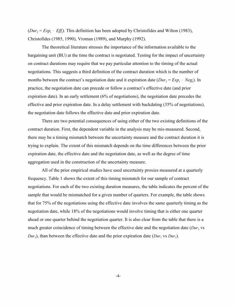
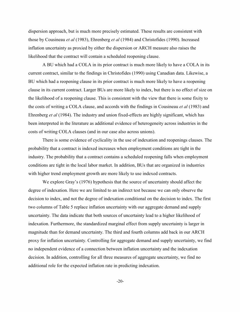
Figure 1 suggests that this may be at variance with the data. Define a “timely settlement” to be

one where the negotiation of the subsequent contract is concluded at the expiration of the current

contract ( Expt-1 = Negt = Efft ). Timely settlements have the feature that all three definitions of the

contract duration are the same. Figure 2 shows a histogram of durations for all timely settlements

pooled across the years of our sample. A clear feature of the data is the prominence of contracts

that are multiples of twelve months in duration. Ninety-three percent of these settlements involve

contracts durations that are multiples of twelve months.4

This pattern of contract durations illustrates the strong desire by many BUs to conduct

their contract renewals during a specific time of the year. This interest (which is outside of the

basic economic model under consideration in this paper) creates an inertia to the decisions of the

BUs regarding the current contract duration. Variations in the prevailing uncertainty at the time

of the negotiations may generate changes in the desired contract durations, but not in the

observed contract durations. That is, the advantages arising from making small adjustments in

the contract duration are outweighed by the disadvantages of departing from the current seasonal

timing of the negotiations.

In addition, when the BU does decide to adjust its contract duration, it is apt to adjust the

duration in a way that maintains the seasonal timing. This can be seen in Figure 3, where we

show the first difference in contract durations, again for the sample of timely settlements. For the

cases where we have adjacent timely settlements, 80% involve no change in the duration. In 74%

of the cases where the duration is adjusted, the change involves a multiple of a year.

5For reasons of data availability, most of the literature has included only an indicator for whethera contract contains a cost-of-living adjustment clause. Christofides and Wilton (1983), Card (1986) andChristofides (1990) examine the degree of indexation.

6A minority of reopening clauses are triggered by a prespecified movement in a cost-of-livingindex, instead of having their date prespecified. These are referred to as COLA reopenings. We lumpthese together with scheduled reopenings since there are too few of them to analyze separately.

-6-

Allowing for some censoring of the underlying desired contract durations can be

accommodated by assuming that the union and firm use the following simple rounding rule. If

the BU chooses to only negotiate at a particular time of year, we assume that they round their

desired contract duration up or down to satisfy that constraint in the way that minimizes the

absolute deviation between the actual and their desired contract duration. For any censored

contract duration, this implies that the unobserved desired duration is in an interval between six

months prior to and six months following the observed contract duration.

3. Indexation and Scheduled Contract Reopenings

The empirical literature has included as an explanatory variable a measure of the

indexation of the contract to changes in the cost-of-living.5 Because cost-of-living adjustment

(COLA) clauses are jointly negotiated along with the length of the contract, the COLA indicator

is treated as endogenous.

There is a second mechanism by which the BU can build flexibility into the contract. A

contract can specify one or more scheduled reopenings for the purpose of negotiating deferred

wage increases. A scheduled reopening differs from an unscheduled reopening. An unscheduled

reopening of the contract can occur at any time during the term of the contract with the mutual

consent of the firm and the union. An unscheduled reopenings requires the firm and the union to

negotiate in “good faith” over all terms and conditions of employment. In contrast, a scheduled

reopening occurs at a prespecified date, and only obligates the firm and the union to negotiate in

good faith over that specific deferred wage increase.6

The existing literature has not controlled for the presence of a reopening clause. The

relative importance of these two forms of contract flexibility for our data is illustrated in Table 2

which shows a cross-tabulation of these two contract provisions. Sixty-three percent of all

7The data ends in 1995 due to the decision by the BLS to stop collecting data on major unioncontracts.

8The correlation between the contract duration and the number of contract negotiations by a BUis >0.33, which is statistically significant.

9Weighting each contract equally gives an overall mean duration of 32.8 months. Weighting eachBU equally gives an overall mean contract duration of 33.8 months.

-7-

contracts in our sample contain neither a COLA nor a reopener clause. The more prevalent type

of flexibility is a COLA clause, which appears in 34% of the contracts. Scheduled reopening

clauses appear in less than 5% of the contracts. Few contracts (less than one percent) contain

both a COLA and a reopener clause.

4. Unbalanced Panel

The data consist of all major contract negotiations followed by the BLS from 1970 to

1995.7 The BLS data provide a unique identification number for each BU, as well as a variable

which tracks each negotiation. Together these two variables provide a panel structure to the data.

The time period covered by different BUs can vary due to either changes in the scope of the

coverage of major collective BUs by the BLS over the sample period, or changes in the size of

the BU.

The nature of the sample implies that on average the number of contract negotiations that

we observe for a specific BU is related to the average length of its contracts. For example, a BU

that negotiates three year contracts can at most have nine observations in the data. In contrast, a

BU that negotiates one year contracts can have up to twenty-five observations. This not only

leads to an unbalanced panel structure, but also implies that the length of each BU’s panel is

inversely related to the variable of interest.8 Allowing each negotiation to have an equal weight

in the estimation would result in over weighting short duration contracts relative to their

importance at any point in time.9 Table 3 shows the sample frequency, median, and mean

contract duration for each panel length in the sample.

10We exclude the contract duration from the list of explanatory variables for the COLA andreopener specifications. See Appendix A for further discussion.

-8-

( )

*

*

*

*

*

1, (0, )

1

1 if 0

0 otherwise

1 if 0

0 otherwise

it it cit

it it rit

cr

cit rit

it

it

it

it

it it it c it r dit

C Z

R M

N

CC

RR

D X C R

γ ε

δ ε

σε ε

β β β ε

= +

= +

Σ Σ =

≥=

≥=

= + + +

�

�

(1)

5. Econometric Framework

These four data considerations can be accommodated in the following econometric

framework:th

th

1 if the contract for BU contains a COLA clause

0 otherwise

1 if the contract for BU contains a reopener clause

0 oth

it

it

t iC

t iR

=

=erwise

We estimate the parameter vectors (γ,δ) using a bivariate probit model. We replace the actual

COLA and reopener indicators with their predicted values when estimating the duration

specification.10

Assuming that εdit is distributed normally with mean zero and standard deviation σd, the

contribution to the overall likelihood from the tth contract for BU i is given by:

11 These papers contrast with the conclusion of Dye (1985) who argues that contract duration isunaffected by uncertainty.

-9-

1

^ ^

^ ^ ^ ^

it

it

I

it itit

I

U Lit it

it c it r

d

it itc it c itr r

d d

D XL

D X D X

C R

C R C R

βφ

σ

β βσ σ

β β

β β β β

−

− −=

− − − −Φ − Φ

−

− −

�

(2)

To address the unbalanced nature of our panel, we set up the likelihood function so that

each BU receives an equal weight. Let Ni denote the number of contract negotiations observed

for the ith BU. Then the contribution of this BU to the overall likelihood, Li, is given as follows:

( )1

1

iNi

N

i itt

L L=

= ∏(3)

III. Measuring Changes in Aggregate Uncertainty Over Time

1. Time-Varying Estimates of Inflation Uncertainty

Theoretical work has identified uncertainty as a key determinant of contract length,

although no consensus has emerged about the sign of the effect. The early papers of Gray (1978),

Canzoneri (1980), and Fethke and Policano (1982) posit a negative relationship between contract

length and uncertainty. On the other hand, Harris and Holmstrom (1987) and Danziger (1988)

predict a positive relationship.11

While the papers listed above principally concern aggregate nominal and real uncertainty,

a number of empirical studies have narrowed the focus to investigate the relationship between the

duration of wage contracts and inflation uncertainty. The lack of direct observations on inflation

12 There is a large empirical literature that has employed forecast dispersion measures fromsurvey series to quantify the effect of inflation uncertainty on aggregate economic activity. These includeCukierman and Wachtel (1979), Levi and Makin (1980), Mullineaux (1980) and Holland (1986, 1993).

-10-

πt�1 � Xtβt � εt�1,

σ2t (π) � E [(ε2

l )], l�1,2 , . . . , t .(4)

σ2t (π) � (1/N)ˆ

N

i�1(πj

it � π̄jt)

2(5)

uncertainty, however, has required these researchers to adopt various methods to measure (and

allow) shifts in the variance of inflation over time.

As one approach, Christofides and Wilton (1983) and Christofides (1985, 1990) specify

an autoregressive process for inflation, and then reestimate the model sequentially by adding

individual observations to the sample. The square of the standard error of the estimate from the

sliding regressions is then used as a proxy for inflation uncertainty. This approach can be

described as follows:

where is the inflation rate between period t and period t+1, is a vector of explanatoryπt�1 Xt

variables (lagged inflation rates) available through period t, βt is the coefficient vector of the

model through period t, is the error term of the model, and is the measure of inflationεt�1 σ2t (π)

uncertainty in period t.

Another approach is to examine survey data on price expectations. This provides direct

measures of inflation expectations, which circumvents possible errors in specifying how people

form their inflation expectations. Researchers have used the dispersion of forecasts across

respondents as a proxy for the variance of inflation.12 Vroman (1989) adopts this procedure and

constructs a measure of inflation uncertainty based on the cross-sectional variance of predicted

price changes from the Livingston survey. This approach can be described by:

where is individual i’s forecast of inflation between period t and period t+j, is theπjit π̄j

t

consensus (average) inflation forecast across the N survey respondents at time t, and j is defined

13Equation (5) accounts for the fact that some survey series involve overlapping data, where theforecast horizon of the survey series is greater than its sampling interval. Overlapping data results in the respondents’ predictions acting as a multi-step-ahead forecast and a value of j that exceeds unity. Whilethis point has no direct bearing on the construction of the forecast dispersion measure in (5), it is relevantfor our subsequent discussion.

14The formulation in (6) can accommodate the use of overlapping data. Overlapping data placesrestrictions on the specification of the ARCH process due to informational considerations, and does notpreclude autocorrelation of the model’s disturbance terms. Rich, Raymond and Butler (1992) provide

-11-

E[εt,j |It ] � E[πt�j� π̄jt |It ] � 0

σ2t (π) � E[ε2

t , j |It ] � ht , j � α0 � ˆp

i�jαiε

2t�i , j

(6)

as the ratio of the forecasting horizon to the sampling interval of the survey data.13 Underlying

this approach is an assumption that consensus among individuals’ point predictions for inflation

is indicative of a high degree of predictive confidence on the their part.

The validity of using proxies based on equation (5) depends critically on the relationship

between disagreement and uncertainty. It is important to note, therefore, that Pagan, Hall and

Trivedi (1983) and Zarnowitz and Lambros (1987) argue that there is little reason to believe that

inferences from the (observed) distribution of point predictions should be informative about the

(subjective) probability distribution of possible outcomes used by individuals to generate their

point predictions. Thus, the relationship between forecast dispersion and forecast uncertainty

remains an untested empirical question.

As an alternative to (5), Rich, Raymond and Butler (1992) propose a survey-based

measure of inflation uncertainty that is directly linked to the predictability of the inflation

process. Drawing on the work of Engle (1982, 1983), Rich, Raymond and Butler model the

conditional variance of the consensus forecast errors an Autoregressive Conditional

Heteroskedasticity (ARCH) process. Specifically, they consider the following two-equation

system to generate a time-varying measure of inflation uncertainty:

where is the rate of inflation between period t and period t+j, is the consensus inflationπt�j εt , j

forecast error from the survey conducted in period t, denotes an information set that includesIt

all information available through time t, and is the variance of conditional on .14 Theht , j εt , j It

details on how estimation of (6) can be conducted within a generalized method of moments framework.

15Rich, Raymond and Butler (1992) find evidence of a positive and statistically significantrelationship between the cross-sectional variance of the survey forecasts and the ARCH estimate ofinflation uncertainty for the SRC survey series. We interpret this evidence as partial justification for theuse of the forecast dispersion measure as a proxy for inflation uncertainty. Unlike Vroman (1989), ouranalysis does not employ data from the Livingston survey series because the survey is conducted on asemi-annual basis and does not coincide with the quarterly frequency of our data.

-12-

key feature of equation (6) is that it explicitly models the conditional variance process, and

thereby provides a natural measure of inflation uncertainty from survey data on expected price

changes.

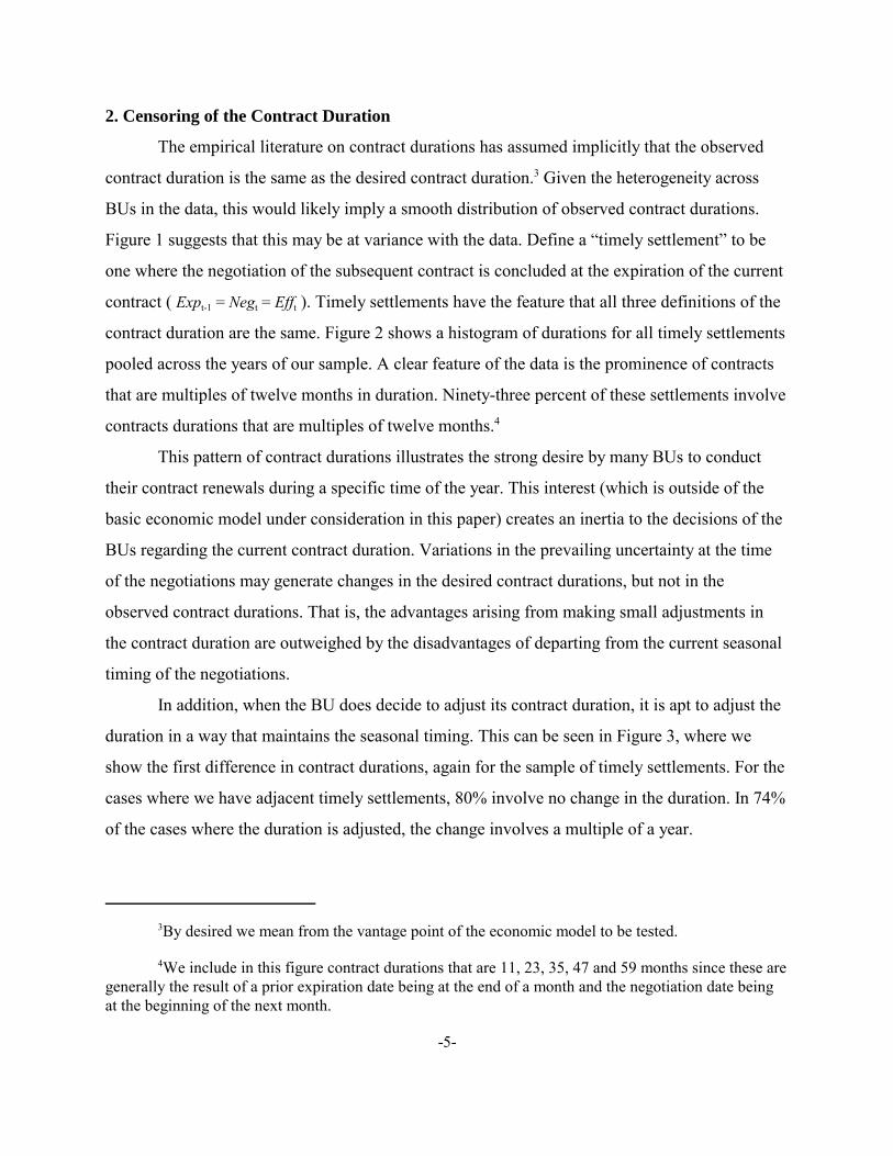
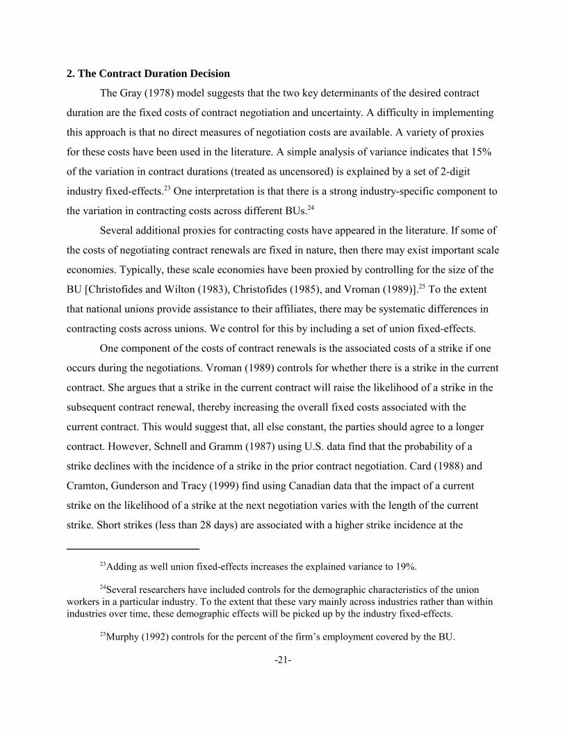
Figure 4 illustrates estimates of inflation uncertainty for the period 1969:Q2-1995:Q3

based on the approaches described in equations (4)-(6). The upper panel plots an estimate of

inflation uncertainty using the sliding regression technique. For purposes of comparison, we also

include a rolling variance measured with a five-year window with equal weights. The five-year

rolling window was applied to the updated residuals from the sliding regressions.

The middle and lower panels of Figure 4 depict estimates of inflation uncertainty using

measures of forecast dispersion and forecast uncertainty from the Survey Research Center (SRC)

expected price change series. The survey series data are quarterly observations on the one-year

CPI inflation forecasts (this implies that j = 4 in equation (6)). The measures of forecast

dispersion and forecast uncertainty correspond, respectively, to the cross-sectional variance of the

survey forecasts and an ARCH estimate of inflation uncertainty.15

Figure 4 illustrates that the estimates of inflation uncertainty can vary considerably across

approaches. Taken together, the measures of forecast dispersion and forecast uncertainty display

the greatest similarity. Specifically, both rise rather dramatically with the food and oil price

shocks of 1973-74 and then generally decline through the middle-1980s and early-1990s. There

is an additional episode of low consensus that coincides with the second round of adverse supply

shocks toward the latter part of the 1970s.

In contrast, the sliding regression technique yields an estimate of inflation uncertainty that

trends slightly upward over the bulk of the sample period. The behavior of this series differs

markedly from the survey-based measures due to its long-term memory process. Because the

16The weights are inversely related to the degrees of freedom in the regression equation. Thisweighting scheme will also act to smooth the inflation uncertainty series as the sample increases.

17Wallace and Blanco (1991) also employ sliding regressions to construct their time-varyingestimates of nominal uncertainty and real uncertainty.

-13-

rolling variance and ARCH estimate of inflation uncertainty depend on the more recent history of

squared forecast errors, their movements are more responsive to variations in the predictability of

the inflation process. However, the sliding regressions generate an estimate of inflation

uncertainty that is a weighted average of all past squared forecast errors.16 As a consequence,

large (squared) forecast errors exert a smaller, but longer-lived influence on this inflation

uncertainty measure. Thus, the increased unpredictability of the inflation process during the

1970s and early 1980s leads to a steady rise in its value, while the increased predictability of

inflation toward the latter part of the sample only translates into a slight decline in its value.

2. Nominal Uncertainty, Real Uncertainty and Structural Vector Autoregressive Models

While the measures of inflation uncertainty in equations (4)-(6) differ in terms of their

construction, there is an issue that concerns each proxy and its inclusion in empirical models of

contract durations. Specifically, the previous discussion abstracted from any consideration of

aggregate nominal and real shocks. If contract length depends in different ways on the source of

uncertainty in an economy, then any attempt to interpret the relationship between contract

duration and inflation uncertainty is problematic due to the influence of both nominal and real

shocks on the behavior of inflation. This consideration would not only be relevant for previous

empirical work, but would also pertain to any study using aggregate uncertainty and inflation

uncertainty interchangeably.

Due to the recognition of this problem, or simply because of their inherent interest in

alternative uncertainty measures, some empirical studies on contract durations have drawn a

distinction between nominal and real shocks. For example, Wallace and Blanco (1991) use

residual-based estimates of money supply shocks and industry-specific productivity shocks to

construct proxies for nominal uncertainty and real uncertainty, respectively.17 While Wallace and

Blanco attempt to account for different types of uncertainty, a potential drawback of their

18The four-variable system is comprised of real output growth, the change in the yield on 3-month Treasury bills, the ex post real return on 3-month Treasury bills, and the growth rate in real moneybalances (measured by M1).

-14-

B(L)Xt � µt(7)

A(L)Xt � εt(8)

approach is that the estimates are based on a single variable which may be too narrow in scope to

serve as a reliable proxy. What is needed, therefore, is an estimation strategy that can be applied

to a set of economic variables, and which offers a more appealing scheme for identifying nominal

and real shocks.

The structural vector autoregression (SVAR) approach offers one such methodology. This

approach uses restrictions based on economic theory to uncover the structural disturbances in an

economy. Within the SVAR framework, Gali (1992) has proposed a four-variable system that

allows for the identification of four structural shocks corresponding to an aggregate supply

shock, an IS shock, a money demand shock, and a money supply shock. Specifically, Gali’s

model is based on the following reduced form VAR:

where X is a vector containing the four variables of the system, isB(L) � In � B1L � . . . � BpLp

a pth-order lag polynomial matrix, is the (4 x 4) identity matrix and is theIn µt � [µ1t , . . . ,µ4t]�

vector of reduced-form errors.18

The structural VAR representation is given by:

where is nonsingular and normalized to have 1's down the main diagonal, andA0 A(L) � A0B(L)

is the (4 x 1) vector of structural disturbances to the system.εt � A0 µt

The ability to disentangle the structural shocks from the reduced-form errors hinges

critically on a set of identification restrictions that allow for the estimation of the matrix . InA0

contrast to other SVAR models that use a recursive system to achieve identification, Gali (1992)

considers a combination of short- and long-run restrictions that focus on the effects of the

19The normalization of the diagonal elements in as well as the assumption that the structuralA0shocks are mutually uncorrelated provide a subset of the restrictions used for identification purposes. SeeGali (1992) for further discussion of the identifying restrictions.

-15-

structural shocks on particular variables.19 The popularity of the Gali model partly stems from its

nonrecursive structure. In addition, the model is capable of generating reasonable responses on

the part of its variables within a relatively low dimensional system.

For our investigation into the determinants of contract duration, the SVAR approach

provides a particularly attractive framework to isolate different sources of uncertainty in the

economy. The IS shock, money demand shock, and money supply shock can be combined into a

composite aggregate demand shock and used to characterize the behavior of nominal

disturbances, while the aggregate supply shock can be interpreted as a real shock. Following

Friedman and Kuttner (1996), we use a rolling window procedure to obtain time-varying

estimates of the variance of nominal and real shocks.

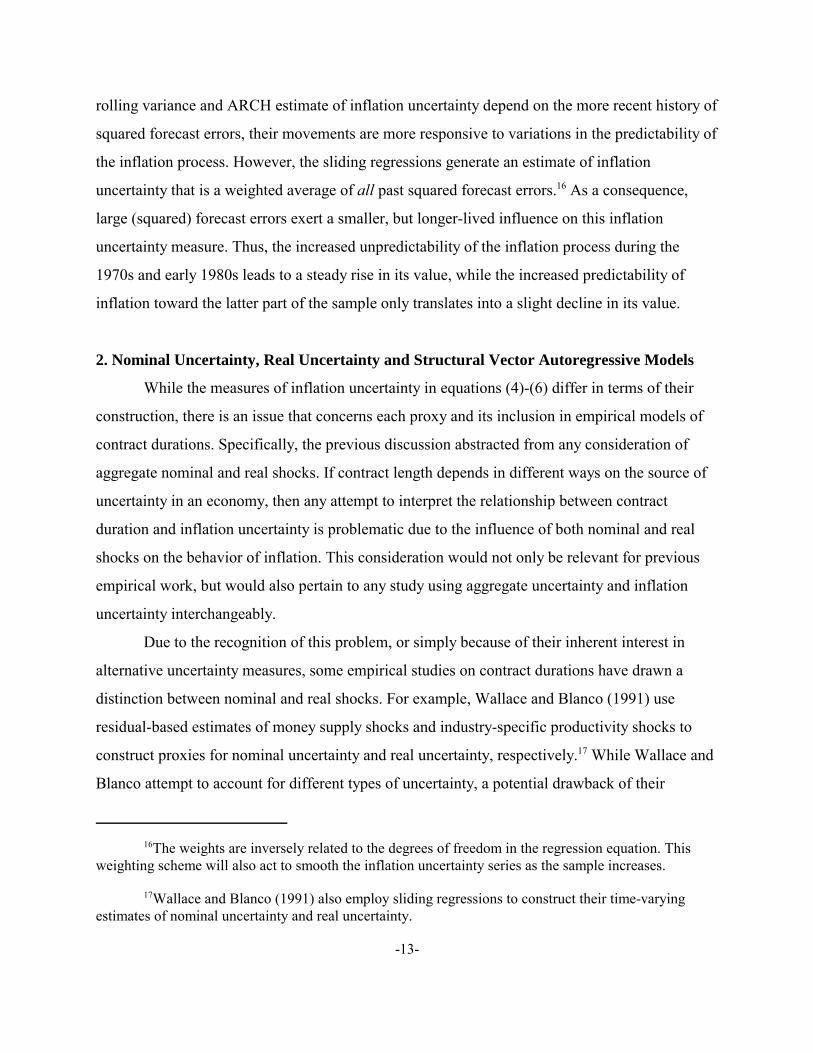
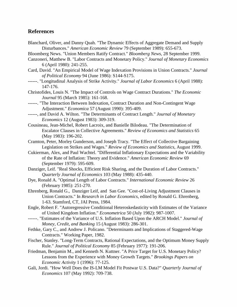
Figure 5 illustrates the estimates of nominal and real uncertainty for the period 1969:Q2-

1995:Q3 from the Gali (1992) model. The moving-average variances are constructed using a

five-year rolling window with equal weights. As is evident from the plots, the variances of these

structural shocks do change over time, as well as relative to each other. Aggregate demand

shocks became increasingly more variable in the late 1970s and early 1980s, and declined sharply

at the outset of the current expansion. In the case of aggregate supply shocks, they are more

variable during the early and mid-1970s, before declining and remaining fairly steady since the

mid-1980s. The patterns in Figure 5 also imply that the uncertainty of nominal shocks relative to

real shocks rose steadily and dramatically through the middle 1980s, before returning to levels

comparable to those at the beginning of the sample period.

An important question is the relative contribution of real and nominal shocks to inflation

uncertainty. To address this issue, we regressed our ARCH inflation uncertainty measure on the

Gali aggregate demand and aggregate supply uncertainty measures. While the results indicate that

inflation uncertainty is positively related to both aggregate demand (nominal) uncertainty and

20However, the evidence indicates that forecast dispersion is positively and statisticallysignificantly related to both nominal and real uncertainty.

21Alternatives would be to scale by some measure of the size of the firm, or the number of BUs atthe firm.

-16-

aggregate supply (real) uncertainty, only the latter yielded evidence of a statistically significant

relationship.20

IV. Empirical Specification and ResultsIn this section, we discuss the additional explanatory variables which we use in

estimating the econometric model outlined in section two. We begin with the bargaining unit’s

(BU’s) decision to adopt a COLA and/or a reopener clause in the current contract. We then turn

our attention to its decision regarding the desired duration of the contract.

1. COLA and Contract Reopeners

The theoretical work on COLA clauses has not explicitly modeled the bargaining process

between a union and a firm. Rather, the literature has adopted the simplifying assumption that the

outcome of this bargaining will be well approximated by an optimal risk-sharing model

[Ehrenberg et al (1984) and Card (1986)]. There are several predictions from this approach

which have guided the empirical literature.

The starting point in the modeling is to assume that there is a fixed cost to writing a

COLA clause into the contract, which suggests that scale economies exist in the use of indexed

contracts. While there are a number of ways to capture these scale economies, we will follow the

literature and control for the size of the BU [Cousineau et al (1983), Ehrenberg et al (1984)].21

Similarly, if a BU had a COLA in its prior contract, the cost of indexing the current contract is

likely to be lower. In most cases, the basic structure of the COLA is maintained between

contracts. This motivates the frequent use of a lag COLA indicator as an instrument for current

indexation [Vroman (1989) and Christofides (1990)]. To the extent that the costs of writing a

COLA vary systematically by industry, the inclusion of industry fixed-effects may be an effective

way to capture this cost variation [Cousineau et al (1983) and Vroman (1989)]. Unions as well

22More specifically, indexation should depend on the correlation between the unexplainedvariance in the index and the unexplained variation in the firm’s output and input prices.

-17-

may develop some expertise in negotiating COLA clauses, which can be passed on to their local

affiliates. In addition to controlling for industry fixed-effects, we also include union fixed-effects

in our specification.

Gray (1976) develops a model in which the optimal degree of indexation depends on the

source of shocks to the economy. Aggregate demand shocks tend to move prices and spot market

wages in the same direction. Indexation, then, helps to maintain the contract wage relative

relation to the spot market wage in response to demand shocks. In contrast, aggregate supply

shocks tend to move prices and spot market wages in opposite directions. For example, a

negative supply shock will tend to push up prices, while lowering the marginal productivity of

labor. Indexation will push the contract wage up when spot market wages are facing downward

pressure. Gray’s analysis suggests that the optimal degree of indexation is increasing in the

importance of aggregate demand shocks relative to aggregate supply shocks. We test this

prediction by separately controlling for nominal and real uncertainty.

Assuming that an indexed contract will use the optimal degree of indexation, Ehrenberg

et al (1984) show that the decision to adopt a COLA depends on the level of inflation

uncertainty, but not on the expected inflation rate over the next contract. Ehrenberg et al (1984)

and Murphy (1992) include both a proxy for expected inflation and inflation uncertainty in order

to test this hypothesis. Vroman (1989) controls for the unexpected inflation rate over the prior

contract and current inflation uncertainty. Cousineau et al (1983) and Christofides (1990) control

for inflation uncertainty, but not the expected inflation rate. We will include proxies for both the

expected inflation rate and inflation uncertainty. In addition, we will explore the sensitivity of the

results to the choice of proxies for inflation uncertainty, and the robustness of the inflation

uncertainty effect when additional proxies for aggregate uncertainty are included.

A central prediction of the risk-sharing framework is that the decision to index and the

degree of indexation should depend in part on the degree of correlation between the COLA index

and the firm’s output and input prices.22 Card (1986) tests for whether the marginal elasticity of

indexation in his sample of Canadian contracts varies with measures of both correlations.

-18-

Hendricks and Kahn (1983), Ehrenberg et al (1984), Christofides (1990) and Murphy (1992)

include measures of the correlation between the consumer price index and the producer price

index for the firm’s industry. A problem with using this control variable in our sample is that

producer price data only exits for some of the industries in our sample, and for some of the years

covered by our sample. Since the literature has not allowed these correlations to be time-varying,

their effects will be picked up by the industry fixed-effects.

Wage and price controls may affect a BU’s decision to index a contract. Cousineau et al

argue that in the case of the Canadian controls, parties have an incentive to index a contract that

has an expiration date following the likely end date of the control period. Wage increases

generated by the COLA clause after the control period ends would not be subject to review. This

suggests that early phases of wage/price controls should have little if any impact on the decision

to index a contract, but that indexation may rise as the expectation of the cessation of controls

begins to set in. Vroman (1989) in her analysis of U.S. labor contracts includes indicators for the

Nixon and Carter control periods.

Several researchers include controls for tightness in the labor market. The choice of the

level of aggregation to use varies across studies. Vroman (1989) uses the aggregate

unemployment rate, Christofides (1990) uses a regional unemployment rate, while Murphy

(1992) uses a state unemployment rate. We follow a hybrid of these approaches by including

measures of tightness in both the local labor market (measured at the state level) and the national

labor market (using the firm’s industry as the reference point).

We control for both trend and cyclical conditions in the state and industry where the BU

is located. We assume that the employment process follows a quadratic time trend, where we

allow for seasonal employment effects and up to a second-order autocorrelation in the errors. We

use BLS state employment data and national industry employment data measured at a quarterly

frequency to estimate the parameters. Letting Eit denote the employment in state or industry i in

period t and Qjt denote quarterly seasonal dummy variables, we estimate the following:

-19-

32

0 1 21

1 1 2 22

log ,

(0, )

it i i i ij jt itj

it it it it

it i

E t t Q

N

β β β δ υ

υ ρ υ ρ υ εε σ

=

− −

= + + + +

= + +

∑

�

(9)

We proxy long-run employment trends in the state or industry by the implied employment

growth, βi1 + 2βi2 t. The composite employment residual, νit, provides a proxy for cyclical

conditions in the state or industry, with tighter labor market conditions represented by larger

residuals.

We use the same set of control variables to model the decision to include a reopening

clause in the contract. As in the case of a COLA clause, we use an indicator for a reopening

clause in the prior contract as an instrument for the presence of a reopening clause. The fixed

costs of writing a reopener clause are likely to be less than the fixed costs of writing a COLA

clause. However, we expect that the presence of a reopener in the prior contract will still increase

the likelihood of having a reopener in the current contract, since the parties are familiar with the

process of negotiating under such a clause.

The results comparing different measures of expected inflation and the level of inflation

uncertainty on the decision to include an indexation and/or reopening clause in the contract are

given in Table 4. The extent to which the indexation decision is sensitive to the source of

aggregate uncertainty is explored in Table 5. Variable sources and summary statistics are given in

the Data Appendix.

The likelihood of indexation increases with both of our measures of expected inflation.

Higher expected inflation, though, does not raise the likelihood of a reopener clause. In contrast,

the inflation uncertainty results are sensitive to the methodology used to construct the uncertainty

measure. The sliding regression methodology generates an uncertainty measure which has a

significant negative effect on the likelihood of a COLA. Using the dispersion of inflation

forecasts as the uncertainty measure produces a positive but insignificant relationship with the

indexation decision. Finally, the ARCH approach produces a quantitatively similar effect as the

-20-

dispersion approach, but is much more precisely estimated. These results are consistent with

those by Cousineau et al (1983), Ehrenberg et al (1984) and Christofides (1990). Increased

inflation uncertainty as proxied by either the dispersion or ARCH measure also raises the

likelihood that the contract will contain a scheduled reopening clause.

A BU which had a COLA in its prior contract is much more likely to have a COLA in its

current contract, similar to the findings in Christofides (1990) using Canadian data. Likewise, a

BU which had a reopening clause in its prior contract is much more likely to have a reopening

clause in its current contract. Larger BUs are more likely to index, but there is no effect of size on

the likelihood of a reopening clause. This is consistent with the view that there is some fixity to

the costs of writing a COLA clause, and accords with the findings in Cousineau et al (1983) and

Ehrenberg et al (1984). The industry and union fixed-effects are highly significant, which has

been interpreted in the literature as additional evidence of heterogeneity across industries in the

costs of writing COLA clauses (and in our case also across unions).

There is some evidence of cyclicality in the use of indexation and reopenings clauses. The

probability that a contract is indexed increases when employment conditions are tight in the

industry. The probability that a contract contains a scheduled reopening falls when employment

conditions are tight in the local labor market. In addition, BUs that are organized in industries

with higher trend employment growth are more likely to use indexed contracts.

We explore Gray’s (1976) hypothesis that the source of uncertainty should affect the

degree of indexation. Here we are limited to an indirect test because we can only observe the

decision to index, and not the degree of indexation conditional on the decision to index. The first

two columns of Table 5 replace inflation uncertainty with our aggregate demand and supply

uncertainty. The data indicate that both sources of uncertainty lead to a higher likelihood of

indexation. Furthermore, the standardized marginal effect from supply uncertainty is larger in

magnitude than for demand uncertainty. The third and fourth columns add back in our ARCH

proxy for inflation uncertainty. Controlling for aggregate demand and supply uncertainty, we find

no independent evidence of a connection between inflation uncertainty and the indexation

decision. In addition, controlling for all three measures of aggregate uncertainty, we find no

additional role for the expected inflation rate in predicting indexation.

23Adding as well union fixed-effects increases the explained variance to 19%.

24Several researchers have included controls for the demographic characteristics of the unionworkers in a particular industry. To the extent that these vary mainly across industries rather than withinindustries over time, these demographic effects will be picked up by the industry fixed-effects.

25Murphy (1992) controls for the percent of the firm’s employment covered by the BU.

-21-

2. The Contract Duration Decision

The Gray (1978) model suggests that the two key determinants of the desired contract

duration are the fixed costs of contract negotiation and uncertainty. A difficulty in implementing

this approach is that no direct measures of negotiation costs are available. A variety of proxies

for these costs have been used in the literature. A simple analysis of variance indicates that 15%

of the variation in contract durations (treated as uncensored) is explained by a set of 2-digit

industry fixed-effects.23 One interpretation is that there is a strong industry-specific component to

the variation in contracting costs across different BUs.24

Several additional proxies for contracting costs have appeared in the literature. If some of

the costs of negotiating contract renewals are fixed in nature, then there may exist important scale

economies. Typically, these scale economies have been proxied by controlling for the size of the

BU [Christofides and Wilton (1983), Christofides (1985), and Vroman (1989)].25 To the extent

that national unions provide assistance to their affiliates, there may be systematic differences in

contracting costs across unions. We control for this by including a set of union fixed-effects.

One component of the costs of contract renewals is the associated costs of a strike if one

occurs during the negotiations. Vroman (1989) controls for whether there is a strike in the current

contract. She argues that a strike in the current contract will raise the likelihood of a strike in the

subsequent contract renewal, thereby increasing the overall fixed costs associated with the

current contract. This would suggest that, all else constant, the parties should agree to a longer

contract. However, Schnell and Gramm (1987) using U.S. data find that the probability of a

strike declines with the incidence of a strike in the prior contract negotiation. Card (1988) and

Cramton, Gunderson and Tracy (1999) find using Canadian data that the impact of a current

strike on the likelihood of a strike at the next negotiation varies with the length of the current

strike. Short strikes (less than 28 days) are associated with a higher strike incidence at the

26Christofides and Wilton (1983) specified a cost-of-adjustment model. However, it is not clearwhy the adjustment costs should depend on the magnitude of the change in the contract duration (giventhat a change is being made).

27As previously noted, an exception is Wallace and Blanco (1991) who attempt to control forboth nominal and real uncertainty.

-22-

contract renewal, while long strikes (more than 50 days) are associated with a lower strike

incidence at the contract renewal. There is no clear connection, then, between the occurrence of a

strike in the current and subsequent contract negotiation.

To the extent that there is a BU-specific component to contracting costs, researchers have

tried to capture this by including the prior contract duration as an additional control variable

[Christofides (1985) and Vroman (1989)]. This approach is problematic if the underlying

specification does not involve controlling for the lag contract duration.26 If the BU-specific error

components are uncorrelated with the control variables, then no bias is induced by ignoring them

in the estimation. If the BU-specific error components are correlated with the control variables

(which seems plausible if they are proxying for negotiating costs), then ignoring them in the

estimation leads to biased estimates. In either situation, though, adding the lag contract duration

involves including an endogenous variable in the model which also leads to biased estimates.

The other key aspect for testing the Gray (1978) model is controlling for uncertainty.

Most of the literature has focused exclusively on proxying for nominal uncertainty [Christofides

and Wilton (1983), Christofides (1985), Vroman (1989) and Murphy (1992).27 The implicit

assumption has been that nominal uncertainty is well captured by a measure of inflation

uncertainty. While various methods for measuring inflation uncertainty have been used, there has

not been a systematic investigation of how sensitive the results are to the specific measure (based

on a given set of contract negotiations). We consider the three basic methodologies previously

examined in section three. We also apply the Gali (1992) methodology to derive aggregate

nominal and real uncertainty measures. This allows us to conduct two important tests. First, we

can determine if the effect of aggregate uncertainty on contract durations differs depending on the

source of the uncertainty. Second, we can assess the extent to which inflation uncertainty

captures the underlying level of nominal uncertainty.

28Wallace and Blanco (1991) use a nominal uncertainty measure derived from a slidingregression of M1 on its lags and seasonal dummy variables. We estimated two uncertainty measures fromthis model. The first averages the squared residuals over the entire sliding estimation period, while thesecond averages the squared residuals over the most recent five years. The first measure had a positiveand significant coefficient in the duration equation, while the second measure had an insignificantcoefficient in the duration equation.

-23-

Christofides (1985) argues that a BU’s desired contract duration will depend on whether

the contract is negotiated during a period of wage and price controls. If there is a perception that

controls will expire in the near future, then there is an incentive for the parties to negotiate a

shorter contract. This will permit them at the renewal to reset the contract terms unconstrained by

the controls. Christofides (1985) tests this prediction using Canadian contract data, while

Vroman (1989) and Wallace and Blanco (1991) investigate this hypothesis using U.S. contract

data.

We also control for conditions in the industry and local labor markets. As we discussed

earlier, we control for trend employment growth in the industry and state, as well as for the

degree to which current employment in the industry and state is above or below its trend.

Vroman (1989) controls for the overall tightness in the labor market using the aggregate

unemployment rate. Murphy (1992) controls for the employment growth rate in the BU’s

industry in the year prior to the contract renewal.

The impact of inflation uncertainty on contract durations is explored in Table 6.

Specification (1) uses the uncertainty measure produced by the sliding regression methodology.

As was evident in Figure 4, this measure behaves quite differently from the dispersion and

ARCH measures. The data indicate no significant relationship between the sliding regression

inflation uncertainty measure and contract durations.28 In contrast, both measures derived from

the SRC survey data generate inflation uncertainty estimates that have a negative and significant

relationship with desired contract durations. The dispersion measure displays a larger

standardized impact than the ARCH measure. There is clear evidence, then, of a negative

relationship between inflation uncertainty (appropriately measured) and contract durations.

In specification (4) of Table 6 we substitute our two aggregate uncertainty measures for

the inflation uncertainty measure. Consistent with the Gray (1978) model and in contrast to the

-24-

predictions from Danziger (1988), we find that both nominal and real uncertainty are associated

with shorter contract durations. The real uncertainty effect is slightly larger in absolute value than

the nominal uncertainty effect, while both are larger than the earlier inflation uncertainty effects.

When we include the ARCH measure of inflation uncertainty with the aggregate demand and

supply uncertainty measures [specification (5) of Table 6], the coefficients on the aggregate

uncertainty measures are relatively unaffected, while the coefficient on inflation uncertainty is no

longer significant.

The aggregate demand uncertainty measure used in specification (4) is a composite built

up from three underlying components: an IS shock, a money demand shock, and a money supply

shock. Table 7 explores the question of whether the negative effect of the composite aggregate

demand uncertainty is being driven primarily by any of its underlying components. The data

indicate a negative, significant and roughly equal effect of uncertainty over each of the three

components on desired contract durations.

A prediction from some models is that after controlling for the uncertainty over future

inflation, the expected inflation rate should have no independent influence on contract durations.

The impact of the expected inflation rate on the desired duration is sensitive to how we control

for inflation uncertainty. When we use the dispersion measure of inflation uncertainty, the

expected rate of inflation has no impact on the desired contract duration. When we use the

ARCH measure of inflation uncertainty, periods of higher expected inflation are associated with

shorter contract durations. Adding the aggregate nominal and real uncertainty measures to the

ARCH inflation uncertainty measure does not eliminate the effect of the expected rate of

inflation on the desired length of contracts. However, when we control for aggregate demand

uncertainty using either our proxy for money supply uncertainty or IS uncertainty, the expected

inflation rate has no additional impact on contract durations.

Contracts which build in flexibility either through indexation or reopening provisions are

associated with longer desired contracts. The effect of a reopening provision is twice the

magnitude of a COLA clause, though less precisely estimated. The data strongly reject for all

specifications the hypothesis that the COLA are reopening clauses are exogenous.

29Christofides and Wilton (1983) can measure not only whether a contract is indexed, but also thedegree of indexation among indexed contracts. They find that the duration response to their inflationuncertainty proxy is larger in absolute magnitude for nonindexed contracts, and that it diminishes withthe contract’s degree of indexation.

-25-

Indexation and reopening clauses may also affect the sensitivity of the desired contract

duration to changes in uncertainty. To explore this, we interact the COLA and scheduled

reopening indicators with the ARCH inflation uncertainty proxy. We find that the negative effect

of increased inflation uncertainty on desired contract durations is entirely driven by the non-

indexed contracts.29 Contracts with schedule reopening clauses have the same sensitivity as

contracts without COLAs and reopenings. We construct similar interactions with the aggregate

demand and supply uncertainty proxies. Here we find that the durations of indexed contracts are

less responsive to aggregate demand and supply uncertainty, but we can reject the hypothesis that

the duration of indexed contracts do not respond to aggregate uncertainty. In contrast, contracts

with scheduled reopenings have durations that are significantly more sensitive to aggregate

demand and supply uncertainty.

The industry and union fixed-effects are jointly significant in every specification. When

we add to the specification an indicator for a short strike in the current contract negotiation, it has

a negative and insignificant effect in all of the specifications. In contrast to the decision to adopt

a COLA clause, there appears to be no significant scale economies in negotiating contracts

associated with larger BUs. Holding the size of the BU constant, we also test for whether BUs

which have experienced membership declines over the prior contract period prefer longer or

shorter contracts. One hypothesis is that BUs faced with membership declines will have a

stronger preference for job security protections to be written into the current contract. This gives

the union an incentive to write a longer contract in order to extend the life of these job

protections. The data suggest that larger membership losses over the prior contract do lengthen

the current contract, though the magnitude of this effect is quite small.

Desired contract durations also vary with cyclical and trend conditions in the industry and

local labor markets. When conditions in the industry are above trend, BUs favor longer contracts.

In contrast, cyclical conditions in the local labor market have no effect on desired contract

durations. This is broadly consistent with Vroman (1989) who finds that tighter aggregate labor

30The expected inflation and ARCH inflation uncertainty in this case are merged in based on theeffective date rather than the negotiation date.

-26-

market conditions as measured by the aggregate unemployment rate lead to longer contracts. In

contrast, stronger trend employment growth in the industry or the local labor market is associated

with shorter contract durations.

Finally, the data indicate that contract durations were shorter during the Nixon wage and

price controls, with the effect being much stronger during Phase II than during the later phases.

There is no systematic evidence that the Carter wage and price controls led to shorter contracts.

Vroman (1989) reports lower contract durations in her sample for both the Nixon and Carter

control periods, with the strongest effects occurring during the Nixon Phase III & IV periods.

Appendix Table A1 explores the sensitivity of the results for specification (3) of Table 6

to the issues of weighting, censoring, and the definition of the contract duration. Specification (2)

of Table A1 weights each contract equally in the estimation. Specification (3) continues to

equally weight all contracts and relaxes the assumption that most observed contract durations are

censored. Specification (4) defines the contract duration to be from the effective date of the

contract to its planned expiration date.30 Finally, specification (5) limits the sample to

manufacturing contracts negotiated prior to 1981. This restricts our sample to roughly the

coverage and time period used by Wallace and Blanco (1991). What emerges from this exercise

is that the weighting, censoring and dating decisions all have meaningful impacts on some of the

estimated coefficients. Restricting the sample to manufacturing contracts negotiated prior to 1981

produces a positive and insignificant coefficient on our ARCH inflation uncertainty measure.

This suggests that part of the reason that the Wallace and Blanco results differ from Vroman

(1989) and Murphy (1992) is that their sample did not capture the changes in contract durations

that began in the mid-1980s.

V. ConclusionsMacro economists have long been interested in understanding the behavior of labor

contracts. These contracts provide a natural source of rigidity in labor markets. By limiting the

actions of the firm and the union during the term of the contract, labor contracts provide a vehicle

-27-

for monetary policy to have short-run real effects [Fischer (1977)]. However, as the degree of

uncertainty in the economy increases, firms and unions should react by shortening the term of

their labor agreements [Gray (1978)]. This endogeneity of the contract duration, if present, would

act to limit the effectiveness of activist monetary policy.

The behavior of labor contracts in practice is an empirical question. Using different

proxies for inflation uncertainty and contract data from different countries, early research built a

case for a robust negative relationship between inflation uncertainty and contract durations

[Christofides and Wilton (1983), Christofides (1985), Vroman (1989) and Murphy (1992)]. On

the other hand, Wallace and Blanco (1991) argued that there was no significant relationship

between U.S. contract durations and inflation uncertainty. In order to resolve this issue, we test

several different measures of inflation uncertainty using a common data set and specification. We

argue that our ARCH uncertainty measure is the preferred proxy, and find that reductions in

inflation uncertainty based on this measure are associated with longer labor contracts. The

empirical relationship is stronger as contracts from the mid-eighties and early nineties are

included in the sample.

Because inflation uncertainty reflects the influence of both real and nominal shocks, we

also investigated the response of contract durations to changes in real and nominal uncertainty.

Risk-sharing models such as Danziger (1988) imply that contracts may increase in length in

response to greater real uncertainty. We provide the first direct test of this hypothesis by using

structural-based estimates of supply (real) and demand (nominal) uncertainty. Consistent with

Gray’s (1978) model, we find that both sources of aggregate uncertainty have a significant

negative relationship with contract durations. Taken together, this evidence suggests that labor

contract durations are endogenous to the economic environment prevailing at the time they are

negotiated, but that risk-sharing concerns are not paramount.

References

Blanchard, Oliver, and Danny Quah. "The Dynamic Effects of Aggregate Demand and SupplyDisturbances." American Economic Review 79 (September 1989): 655-673.

Bloomberg News. "Union Members Ratify Contract." Bloomberg News, 28 September 1999.Canzoneri, Matthew B. "Labor Contracts and Monetary Policy." Journal of Monetary Economics

6 (April 1980): 241-255.Card, David. "An Empirical Model of Wage Indexation Provisions in Union Contracts." Journal

of Political Economy 94 (June 1986): S144-S175.------. "Longitudinal Analysis of Strike Activity." Journal of Labor Economics 6 (April 1988):

147-176.Christofides, Louis N. "The Impact of Controls on Wage Contract Durations." The Economic

Journal 95 (March 1985): 161-168.------. "The Interaction Between Indexation, Contract Duration and Non-Contingent Wage

Adjustment." Economica 57 (August 1990): 395-409.------, and David A. Wilton. "The Determinants of Contract Length." Journal of Monetary

Economics 12 (August 1983): 309-319.Cousineau, Jean-Michel, Robert Lacroix, and Banielle Bilodeau. "The Determination of

Escalator Clauses in Collective Agreements." Review of Economics and Statistics 65(May 1983): 196-202.

Cramton, Peter, Morley Gunderson, and Joseph Tracy. "The Effect of Collective BargainingLegislation on Strikes and Wages." Review of Economics and Statistics, August 1999.

Cukierman, Alex, and Paul Wachtel. "Differential Inflationary Expectations and the Variabilityof the Rate of Inflation: Theory and Evidence." American Economic Review 69(September 1979): 595-609.

Danziger, Leif. "Real Shocks, Efficient Risk Sharing, and the Duration of Labor Contracts."Quarterly Journal of Economics 103 (May 1988): 435-440.

Dye, Ronald A. "Optimal Length of Labor Contracts." International Economic Review 26(February 1985): 251-270.

Ehrenberg, Ronald G., Danziger Leif, and San Gee. "Cost-of-Living Adjustment Clauses inUnion Contracts." In Research in Labor Economics, edited by Ronald G. Ehrenberg,1-63. Stamford, CT, JAI Press, 1984.

Engle, Robert F. "Autoregressive Conditional Heteroskedasticity with Estimates of the Varianceof United Kingdom Inflation." Econometrica 50 (July 1982): 987-1007.

------. "Estimates of the Variance of U.S. Inflation Based Upon the ARCH Model." Journal ofMoney, Credit, and Banking 15 (August 1983): 286-301.

Fethke, Gary C., and Andrew J. Policano. "Determinants and Implications of Staggered-WageContracts." Working Paper, 1982.

Fischer, Stanley. "Long-Term Contracts, Rational Expectations, and the Optimum Money SupplyRule." Journal of Political Economy 85 (February 1977): 191-206.

Friedman, Benjamin M., and Kenneth N. Kuttner. "A Price Target for U.S. Monetary Policy?Lessons from the Experience with Money Growth Targets." Brookings Papers onEconomic Activity 1 (1996): 77-125.

Gali, Jordi. "How Well Does the IS-LM Model Fit Postwar U.S. Data?" Quarterly Journal ofEconomics 107 (May 1992): 709-738.

Gamboa, Glenn. "Goodyear Union Members in Fayetteville Approve Contract, Return to Work."Akron Beacon Journal, 8 May 1997.

Gray, Jo Anna. "Wage Indexation: A Macroeconomic Approach." Journal of MonetaryEconomics 2 (April 1976): 221-35.

------. "On Indexation and Contract Length." Journal of Political Economy 86 (February 1978):1-18.

Harris, Milton, and Bengt Holmstrom. "On the Duration of Agreements." InternationalEconomic Review 28 (June 1987): 389-406.

Heckman, James. "Dummy Endogenous Variables in a Simultaneous Equation System."Econometrica 46 (July 1978): 931-959.

Hendricks, Wallace E., and Lawrence M. Kahn. "Cost-of-Living Clauses in Union Contracts:Determinants and Effects." Industrial and Labor Relations Review 36 (April 1983):447-460.

Holland, Steven A. "Wage Indexation and the Effect of Inflation Uncertainty on Unemployment:An Empirical Analysis." American Economic Review 76 (March 1986): 235-243.

------. "Uncertain Effects of Money and the Link Between the Inflation Rate and InflationUncertainty." Economic Inquiry 31 (January 1993): 39-51.

Hyde, Justin. "UAW Gives Ford Right to Spin Off Visteon Plants - Not Workers." TheAssociated Press, October 14 1999.

Juster, F. Thomas, and Robert Comment. "A Note on the Measurement of Price Expectations."Mimeo. University of Michigan Research Center, 1980.

Levi, Maurice D., and John H. Makin. "Inflation Uncertainty and the Phillips Curve: SomeEmpirical Evidence." American Economic Review 70 (December 1980): 1022-1027.

Mullineaux, Donald J. "Unemployment, Industrial Production, and Inflation Uncertainty in theUnited States." Review of Economics and Statistics 62 (May 1980): 163-169.

Murphy, Kevin J. "Determinants of Contract Duration in Collective Bargaining Agreements."Industrial and Labor Relations Review 45 (January 1992): 352-365.

Pagan, Adrian R., Alistar D. Hall, and Pravin K. Trivedi. "Assessing the Variability of Inflation."Review of Economic Studies 50 (October 1983): 585-596.

Phillips, David, and Peronet Despeignes. "Costs May Outweigh UAW Gains: Automakers Waitfor Results of Four-Year Contracts With Union." The Detroit News, 27 October 1999.

Rich, Robert W., Jennie E. Raymond, and J.S. Butler. "The Relationship Between ForecastDispersion and Forecast Uncertainty: Evidence From a Survey-Data ARCH Model."Journal of Applied Econometrics 7 (April 1992): 131-148.

Schnell, John F., and Cynthia L. Gramm. "Learning by Striking: Estimates of the TeetotalerEffect." Journal of Labor Economics 5 (April 1987): 221-241.

Taylor, John B. "Aggregate Dynamics and Staggered Contracts." Journal of Political Economy88 (February 1980): 1-23.

Thomson, Linda. "Kennecott Workers Ratify Pact." The Desert News, 25 October 1996.Vroman, Susan. "Inflation Uncertainty and Contract Duration." Review of Economics and

Statistics 71 (November 1989): 677-681.Wallace, Frederick H., and Hermino Blanco. "The Effects of Real and Nominal Shocks on

Union-Firm Contract Duration." Journal of Monetary Economics 27 (June 1991):361-380.

Zarnowitz, Victor, and Louis A. Lambros. "Consensus and Uncertainty in EconomicPredictions." Journal of Political Economy 95 (June 1987): 591-621.

10th

25th

50th75th

90th

Months

Year1975 1980 1985 1990 1995

0

20

40

60

Figure 1. Evolution of Contract Durations

Notes: Private sector labor contracts covering at least 1,000 workers. Duration is measured from theeffective date to the expiration date.

Fra

ctio

n

Contract duration (months)12 24 36 48 60

0

.2

.4

.6

Fra

ctio

n

Change in contract duration-36 -24 -12 0 12 24 36

0

.2

.4

.6

.8

Figure 2. Distribution of Contract Durations - Timely Settlements

Figure 3. Distribution of the Change in Contract Durations - Timely Settlements

Sliding Regression Measure - 1969:Q2 - 1995:Q3

Year1970 1975 1980 1985 1990 1995

0

2

4

6

Rolling Variance

SEE Squared

SRC Survey Forecast Dispersion Measure - 1969:Q2 - 1995:Q3

Year1970 1975 1980 1985 1990 1995

0

50

100

150

SRC Survey ARCH Measure - 1969:Q2 - 1995:Q3

Year1970 1975 1980 1985 1990 1995

0

5

10

15

Figure 4. Alternative Measures of Inflation Uncertainty

Note: Dates on the horizontal axis correspond to the end of the five-year window in the top panel.

Aggregate Demand: 1969:Q2 - 1995:Q3

Year1970 1975 1980 1985 1990 1995

0

2

4

6

8

Aggregate Supply: 1969:Q2 - 1995:Q3

Year1970 1975 1980 1985 1990 1995

.5

1

1.5

2

2.5

Figure 5. Variances of Structural Shocks > Gali Model

Note: Dates on the horizontal axis correspond to the end of the five-year window.

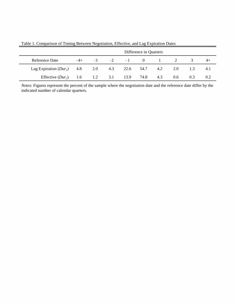
Table 1. Comparison of Timing Between Negotiation, Effective, and Lag Expiration Dates

Difference in Quarters

Reference Date >4+ >3 >2 >1 0 1 2 3 4+

Lag Expiration (Dur1) 4.8 2.0 4.3 22.6 54.7 4.2 2.0 1.3 4.1

Effective (Dur2) 1.6 1.2 3.1 13.9 74.8 4.3 0.6 0.3 0.2

Notes: Figures represent the percent of the sample where the negotiation date and the reference date differ by theindicated number of calendar quarters.

Table 2. Distribution of COLA and Reopener Clauses

Reopener Clause

No Yes

COLA Clause No 61.3 4.7

Yes 33.3 0.7

Notes: Numbers indicate the percent of contracts which have theindicated combination of COLA and reopener clauses.

Table 3. Panel Lengths and Contract Durations

Panel Length% of

Sample% of BUs

MedianDuration

MeanDuration

1 1.37 7.67 35 37.8

2 1.75 4.89 35 33.7

3 5.30 9.87 35 35.2

4 9.90 13.83 36 34.3

5 8.61 9.61 35 33.5

6 13.05 12.14 35 33.4

7 24.63 19.65 35 35.3

8 19.81 13.83 35 33.2

9 5.98 3.71 26.5 28.6

10 4.53 2.53 23 26.1

11 2.49 1.26 24 23.8

12+ 2.58 1.01 12 16.0

Notes: Sample restricted to the set of contracts used in theestimation.

Table 4. Bivariate Probit - COLA and Reopener Clause, Expected Inflation and Inflation Uncertainty

Variable COLA Reopener COLA Reopener COLA Reopener

Lag COLA 2.093**

(0.060)>0.132(0.100)

2.029**

(0.058)>0.160(0.103)

2.040**

(0.058)>0.144(0.101)

Lag reopener 0.040(0.128)

1.117**

(0.104)0.047

(0.128)1.111**

(0.105)0.043

(0.129)1.123**

(0.105)

Log BU Size 0.098**

(0.024)>0.006(0.039)

0.106**

(0.024)>0.002(0.039)

0.105**

(0.024)>0.003(0.039)

Expected inflation: • Regression forecast 0.219**

(0.041)0.003

(0.056)

• SRC survey concensus 0.277**

(0.077)>0.051(0.091)

0.302**

(0.039)0.044

(0.051)

Inflation uncertainty: • Regression SEE >0.240**

(0.035)>0.087(0.050)

• SRC - dispersion of forecasts 0.064(0.067)

0.150*

(0.083)

• SRC - ARCH 0.074**

(0.025)0.080**

(0.029)

State employment residual >0.022(0.025)

>0.114**

(0.032)>0.013(0.025)

>0.112**

(0.031)>0.010(0.025)

>0.113**

(0.032)

State employment trend 0.037(0.026)

0.077**

(0.033)0.042

(0.027)0.077**

(0.033)0.038

(0.027)0.075**

(0.033)

Industry employment residual 0.080**

(0.024)>0.020(0.031)

0.100**

(0.024)>0.020(0.031)

0.105**

(0.024)>0.016(0.030)

Industry employment trend 0.060(0.116)

0.155(0.160)

0.289**

(0.120)0.201

(0.165)0.259**

(0.120)0.165

(0.165)

Nixon phase II >0.086(0.678)

0.835(0.774)

0.973(0.673)

1.284*

(0.763)0.982

(0.664)1.258

(0.769)

Nixon phase III & IV >0.528**

(0.191)0.129

(0.208)>0.109(0.165)

0.233(0.185)

>0.189(0.167)

0.156(0.185)

Carter phase I >0.515**

(0.133)0.242

(0.168)>0.792**

(0.139)0.082

(0.175)>0.728**

(0.140)0.181

(0.175)

Carter phase II >0.089(0.145)

>0.073(0.213)

>0.146(0.125)

>0.203(0.176)

>0.099(0.127)

>0.137(0.178)

Rho >0.307**

(0.062)>0.295**

(0.062)>0.306**

(0.062)

Notes: Standard errors are given in parentheses and have been adjusted for any nonindependence across contracts in thesame BU. Sample size is 6,524. Continuous RHS variables have been standardized to have a zero mean and unit standarddeviation. All specifications control for 2-digit industry fixed effects and 43 union fixed effects.** significant at the 5% level * significant at the 10% level

Table 5. Bivariate Probit - COLA and Reopener Clause, Aggregate Demand and Supply Uncertainty

Variable COLA Reopener COLA Reopener

Expected inflation: • SRC survey consensus 0.081*

(0.045)0.076

(0.058)0.070

(0.045)0.045

(0.058)

Uncertainty: • Aggregate demand 0.148**

(0.040)0.093*

(0.053)0.145**

(0.040)0.087

(0.053)

• Aggregate supply 0.527**

(0.054)0.109

(0.072)0.518**

(0.054)0.087

(0.073)

• Inflation, SRC - ARCH 0.031(0.026)

0.078**

(0.029)

Notes: Standard errors are given in parentheses and have been adjusted for any nonindependenceacross contracts in the same BU. Sample size is 6,524. Continuous RHS variables have beenstandardized to have a zero mean and unit standard deviation. All specifications control for 2-digitindustry fixed effects and 43 union fixed effects.** significant at the 5% level * significant at the 10% level

Table 6. Contract Durations - Inflation, Aggregate Demand & Supply Uncertainty

Variable (1) (2) (3) (4) (5)

COLA1 1.17*

(0.062)1.43**

(0.63)1.31**

(0.62)1.65**

(0.60)1.65**

(0.60)

Reopener1 3.23(2.43)

3.23(2.44)

3.81(2.36)

3.99*

(2.35)4.18*

(2.37)

Log BU Size 0.06(0.19)

0.06(0.19)

0.07(0.18)

0.06(0.18)

0.06(0.19)

Percent change in BU size(negative changes)

0.18(0.13)

0.17(0.13)

0.16(0.13)

0.22*

(0.13)0.22*

(0.13)

Expected inflation: • Regression forecast >1.15**

(0.29)

• SRC survey consensus >0.03(0.39)

>1.11**

(0.29)>0.61*

(0.30)>0.59*

(0.30)

Inflation uncertainty: • Regression SEE >0.03

(0.19)

• SRC - dispersion of forecasts >1.25**

(0.40)

• SRC - ARCH >0.33**

(0.11)>0.12(0.12)

Aggregate uncertainty: • Aggregate demand >2.05**

(0.34)>2.03**

(0.34)

• Aggregate supply >2.66**

(0.35)>2.62**

(0.36)

Table 6. Continued

Variable (1) (2) (3) (4) (5)

State employment residual >0.13(0.13)

>0.22(0.14)

>0.15(0.13)

>0.01(0.13)

>0.02(0.13)

State employment trend >0.74**

(0.20)>0.72**

(0.19)>0.72**

(0.19)>0.58**

(0.19)>0.58**

(0.19)

Industry employment residual 0.74**

(0.22)0.69**

(0.22)0.70**

(0.22)0.65**

(0.21)0.64**

(0.21)

Industry employment trend >3.74**

(1.12)>3.36**

(1.20)>3.23**

(1.21)>0.58(1.39)

>0.58(1.39)

Nixon phase II >10.94**

(4.82)>11.78**

(4.79)>11.72**

(4.79)>11.76**

(4.82)>11.91**

(4.82)

Nixon phase III & IV >1.54*

(0.92)>1.43*

(0.93)>1.04(0.95)

>1.01(0.94)

>0.88(0.95)

Carter phase I 0.39(0.52)

1.09*

(0.58)0.88

(0.57)0.02

(0.57)>0.03(0.57)

Carter phase II 1.22**

(0.60)0.34

(0.38)0.26

(0.38)>1.09**

(0.38)>1.12**

(0.38)

Notes: Standard errors are given in parentheses and have been adjusted for anynonindependence across contracts in the same BU. Sample size is 6,524. ContinuousRHS variables have been standardized to have a zero mean and unit standard deviation.All specifications control for 2-digit industry fixed effects and 43 union fixed effects.1 Predicted values used** significant at the 5% level * significant at the 10% level

Table 7. Decomposition of Aggregate Uncertainty

Variable (1) (2) (3) (4)

Expected inflation - SRC survey consensus >0.61*

(0.30)>0.74**

(0.31)>0.05(0.27)

>0.07(0.28)

Aggregate demand uncertainty• Composite >2.05**

(0.34)

• Money supply uncertainty >1.47**

(0.19)

• Money demand uncertainty >1.45**

(0.18)

• IS uncertainty >1.33**

(0.16)

Aggregate supply uncertainty >2.66**

(0.35)>1.80**

(0.22)>1.88**

(0.24)>1.75**

(0.23)

Notes: Standard errors are given in parentheses and have been adjusted for any nonindependenceacross contracts in the same BU. Sample size is 6,524. Continuous RHS variables have beenstandardized to have a zero mean and unit standard deviation. All specifications control for 2-digitindustry fixed effects and 43 union fixed effects.1 Predicted values used** significant at the 5% level * significant at the 10% level

Table A1. Contract Durations - Sensitivity Analysis

Variable(1)

Baseline

(2)

Unweighted

(3)No

Censoring2

(4)Effective

Date3

(5)Mfg,

1970-19804

COLA1 1.31**

(0.62)1.84**

(0.57)2.73**

(0.60)2.98**

(0.60)6.17**

(1.01)

Reopener1 3.81(2.36)

4.75**

(2.40)3.10

(2.17)3.26

(2.16)1.21

(3.55)

Log BU Size 0.07(0.18)

0.21(0.15)

0.19(0.15)

0.20(0.15)

>0.26(0.21)

Percent change in BU size(negative changes)

0.16(0.13)

0.18*

(0.10)0.20**

(0.10)0.25**

(0.10)0.35

(0.22)

Expected inflation: • SRC survey consensus

>1.11**

(0.29)>0.92**

(0.19)>0.91**

(0.18)>0.92**

(0.18)0.22

(0.39)

Inflation uncertainty: • SRC - ARCH

>0.33**

(0.11)>0.32**

(0.10)>0.27**

(0.10)>0.24**

(0.10)0.09

(0.17)

State employment residual >0.15(0.13)

>0.09(0.12)

>0.13(0.12)

>0.12(0.12)

>0.13(0.27)

State employment trend >0.72**

(0.19)>0.65**

(0.19)>0.73**

(0.19)>0.65**

(0.19)0.21

(0.25)

Industry employment residual 0.70**

(0.22)0.72**

(0.12)0.69**

(0.12)0.78**

(0.12)0.05

(0.30)

Industry employment trend >3.23**

(1.21)>4.20**

(0.82)>3.95**

(0.82)>4.26**

(0.80)>2.50(2.87)

Nixon phase II >11.72**

(4.79)>8.80*

(5.35)>10.17*

(5.56)>9.58*

(5.25)>7.62(4.79)

Nixon phase III & IV >1.04(0.95)

>1.30*

(0.79)>1.38*

(0.77)>2.34**

(0.84)>1.88**

(0.89)

Carter phase I 0.88(0.57)

0.31(0.49)

0.50(0.48)

0.56(0.50)

>0.11(0.83)

Carter phase II 0.26(0.38)

>0.10(0.37)

>0.15(0.37)

>0.12(0.30)

0.53(0.48)

Notes: Standard errors are given in parentheses and have been adjusted for any nonindependence acrosscontracts in the same BU. Sample size is 6,524. Continuous RHS variables have been standardized to havea zero mean and unit standard deviation. All specifications control for 2-digit industry fixed effects and 43union fixed effects.1 Predicted values used2 Maintain equal weighting of all contract negotiations3 Maintain equal weighting of all contract negotiations and assume no censoring.4 Maintain equal weighting of all contract negotiations, assume no censoring and use effective date.** significant at the 5% level * significant at the 10% level

Appendix A: Econometric Specification Issues

In this appendix we provide additional details regarding the econometric specification weestimate. A natural framework is to allow for contract durations to depend onindexation/reopening clauses and vice versa. Our specification only allows the duration decisionto depend on the presence or absence of indexation and/or reopening clauses. There is nofeedback between the desired contract duration and the decisions to include these clauses in thecontract. The rationale for this restriction is detailed below.

Heckman (1978) discusses the following general framework.* *1 1 1 1 2 1 1

* *2 2 2 2 1 2 2

*21 iff 0

0 otherwise

i i i i i

i i i i i

ii

y x d y uy x d y u

yd

α β γα β γ

= + + +

= + + +

>=

where the y variables are potentially unobserved latent variables, and the x variables are assumedto be exogenous. Heckman shows that this is a valid statistical framework if and only ifγ2β1 + β2 = 0.

Consider a simplified version of our model. Ignoring the issue of censoring of somecontract durations and the presence of reopening provisions, we can write our basic specificationinto Heckman’s framework.

*1 1 1 1 1

*2 2 2 2 2

*1 if 00 otherwise

it it it it i

it it it it i

itit

D X C C uC X C D u

CC

α β γα β γ

= + + +

= + + +

>=

Here we assume that the contract duration is observed.Consider first the contract duration equation. In the general framework, both the presence

of a COLA clause as well as the underlying latent variable affecting the indexation decision areallowed to influence the contract duration decision. In this specific application, it is reasonable toallow the presence of a COLA to affect the length of a contract since it provides additionalflexibility (β1 £ 0). However, there is little reason to believe that variation in the latent variableC* would have any independent influence on the contract duration (γ1 = 0).

Turn now to the specification of the latent variable governing the indexation decision.There is little justification in this context to assume that a COLA clause would shift the latentvariable C*. This suggests that we set β2 to zero. Heckman’s restriction is that γ2β1 + β2 = 0. Forthis restriction to be satisfied, we drop D from the equation (set γ 2= 0).

Data Appendix B

Data Definitions and Sources

Sliding Regression Technique. Inflation is measured as the quarterly growth (at an annualrate) in the consumer price series PCU. The slidingregressions are initially estimated using a sample coveringthe period 1966:Q2-1969:Q3.

Expected InflationThe expected inflation series is computed according toequation (5), where the conditional mean of the inflationprocess is specified as an AR(4) process.

Inflation UncertaintyThe inflation uncertainty measure is computed according toequation (5) as the square of the standard error of theestimate.

The Survey Research Center (SRC) Expected Price ChangeSeries. The SRC survey is conducted at the University of Michiganand actually begins in 1948, but has undergone changes inboth the sampling interval and in the form of the surveyquestionnaire. We restrict our attention to post-1966:Q2data because this corresponds to a transition in the survey tocomplete closed-end quantitative data. In addition, thesurvey made a transition from quarterly data to monthlydata in 1977. Therefore, we examine data corresponding tothe months of February, May, August and November tomaintain consistency in the dates of the surveys. Furtherdetails on the SRC survey series are provided in Juster andComment (1980) and Rich, Raymond and Butler (1992).

Expected InflationMeasures of expected inflation are forecasts of CPI inflationover the next year.

Inflation Uncertainty - Forecast Dispersion MeasureThe forecast dispersion measure is computed according toequation (6) as the cross-sectional variance of the inflationforecasts.

Summary Statistics Mean Standard Deviation

5.79 2.96

3.86 0.46

6.08 2.13

56.86 23.64

Data Definitions and Sources

Inflation Uncertainty - ARCH MeasureThe inflation uncertainty measure is computed according toequation (7). The forecast error is constructed as thedifference between the annual rate of change in theconsumer price series PCU and the consensus inflationforecast. The ARCH specification includes the fourth laggedsquared forecast error and is estimated using data from the1968:Q2-1995:Q3 surveys.

3. Gali (1992) Model. All data are quarterly and theestimation is conducted over the sample period 1959:Q1-1995:Q4.

OutputThe output series GDPH is measured as real gross domesticproduct in chain-weighted 1992 dollars.

PricesThe price data are a quarterly average of the monthlyconsumer price series PCU for all urban consumers.

Interest RatesThe interest rate data are a quarterly average of the monthlyseries FTBS3 which represents the yield on three-monthTreasury Bills.

Money StockThe data on the money stock are for M1 and are a quarterlyaverage of the series FM1. The measures of M1 prior to1959 are taken from the Federal Reserve Bulletin.

Aggregate Real and Nominal UncertaintyThe measure of real uncertainty is computed as a rollingvariance of the aggregate supply shock with a five-yearwindow with equal weights. The measure of nominaluncertainty is computed as a rolling variance of a compositeaggregate demand shock with a five-year window with equalweights.

Aggregate Supply

Aggregate Demand

IS Shock

Money Demand Shock

Money Supply Shock

Summary Statistics Mean Standard Deviation

3.42 2.07

0.98 0.48

3.76 1.80

1.40 0.67

1.40 0.83

1.19 0.45

Data Definitions and Sources

Contract DurationThe uncensored duration is measured as the number ofmonths between the negotiation date of the contract and theexpected expiration date. Source: BLS Major Agreementfile.

Cost-of-Living ClauseIndicator taking a value of one if the current contractcontains a cost-of-living adjustment clasue. Source: BLSMajor Agreement file.

Reopening ClauseIndicator taking a value of one if the current contractcontains either one or more scheduled reopening clauses ora cost-of-living reopening clause. Source: BLS MajorAgreement file.

Bargaining Unit SizeLog of the number of workers covered by the laborcontract. Source: BLS Major Agreement file.

Percent Reduction in Bargaining Unit SizeMaximum of zero and the percent change in the size of thebargaining unit between the current contract and the priorcontract. Source: BLS Major Agreement file.

State Employment ResidualResidual from a regression of quarterly log state privatesector nonagricultural employment on a quadratic trend andquarterly seasonal indicators. See equation (10) in text.Source: BLS Employment and Earnings: States & Areasdata.

State Employment TrendTrend growth rate of quarterly state employment impliedfrom equation (10) in text. Source: BLS Employment andEarnings: States & Areas data.

Summary Statistics Mean Standard Deviation 32.74 9.11

0.35 0.48

0.04 0.21

7.94 0.93

9.22 15.26

!0.002 0.028

0.004 0.002

Data Definitions and Sources

Industry Employment ResidualResidual from a regression of quarterly log 2-digit industryemployment on a quadratic trend and quarterly seasonalindicators. See equation (10) in text. Source: BLSEmployment and Earnings: National data.

Industry Employment TrendTrend growth rate of quarterly 2-digit industry employmentimplied from equation (10) in text. Source: BLSEmployment and Earnings: National data.

Wage & Price Controls:

Nixon Phase IIIndicator taking a value of one for contracts negotiatedbetween 1 August 1971 and 31 December 1972.

Nixon Phase III & IVIndicator taking a value of one for contracts negotiatedbetween 1 January 1973 and 30 April 1974.

Carter Phase IIndicator taking a value of one for contracts negotiatedbetween 1 November 1978 and 31 December 1979.

Carter Phase IIIndicator taking a value of one for contracts negotiatedbetween 1 January 1980 and 31 August 1980.

Summary Statistics Mean Standard Deviation 0.002 0.005

!0.002 0.066

0.00 0.02

0.02 0.15

0.05 0.22

0.05 0.21