uncertainty and sensitivity analysis...introduction: sensitivity analysis framework step a...
TRANSCRIPT

Uncertainty and Sensitivity Analysis
Computational Methods for Safety and Risk Analysis A+B

1. Introduction & framework
2. Local approaches:
▪ One-factor-at-a-time sensitivities on the nominal range
o Tornado diagram to spider plot
o Elementary effect & elasticity measures
▪ Morris’ method
3. Global/probabilistic approaches:
▪ Discrete:
o Event and probability tree
o Method of discrete probabilities
▪ Continuous:
o Method of moments
o Regression-based method
• Input/output correlation coefficients
• SRC/SRRC
o Distribution-based method
• Variance decomposition method
• Moment-independent method
4. Model structure uncertainty
Outline
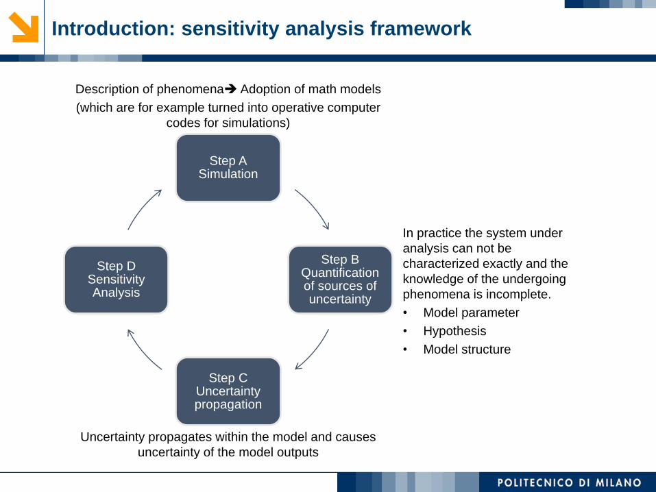
Introduction: sensitivity analysis framework
Step ASimulation
Step BQuantification of sources of uncertainty
Step CUncertainty propagation
Step DSensitivity Analysis
Description of phenomena➔ Adoption of math models
(which are for example turned into operative computer
codes for simulations)
In practice the system under
analysis can not be
characterized exactly and the
knowledge of the undergoing
phenomena is incomplete.
• Model parameter
• Hypothesis
• Model structure
Uncertainty propagates within the model and causes
uncertainty of the model outputs

• Uncertainty analysis and propagation:
propagates the uncertainties of the input parameters and the model structure to the
model output
• Parameter prioritization:
identify the most influential inputs to the output uncertainty
➔more information on those parameters would lead to the largest reduction in the
output uncertainty
• Parameter fixing:
determine non-influential inputs that can be fixed at certain values
➔model simplification
• Direction of change (trend):
whether an increase in an input causes an increase (decrease) in the model output
• Insights about model structure
interactions, etc.
Introduction: objectives of sensitivity analysis

Introduction: how uncertainty propagates
𝒚 = 𝑚(𝒙)
𝒙 = (𝑥1, 𝑥2, … , 𝑥𝑛) : vector of 𝑛 input parameters
𝒚 : output vector correspondent to 𝒙 and 𝑚(𝒙)
𝑚 𝒙 : model structure
• Deterministic (e.g., advection-dispersion equation, Newton law)
• Stochastic (e.g., Poisson model, exponential model)
𝑚(𝒙)
𝒙 = (𝑥1, 𝑥2, … , 𝑥𝑛) 𝒚
𝑚 𝒙

LOCAL APPROACHES
• Tornado diagram to spider plots
• Elementary effect & elasticity measures
• Morris’ method
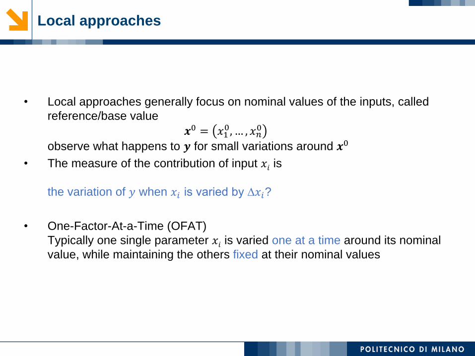
• Local approaches generally focus on nominal values of the inputs, called
reference/base value
𝒙0 = 𝑥10, … , 𝑥𝑛
0
observe what happens to 𝒚 for small variations around 𝒙0
• The measure of the contribution of input 𝑥𝑖 is
the variation of 𝑦 when 𝑥𝑖 is varied by ∆𝑥𝑖?
• One-Factor-At-a-Time (OFAT)
Typically one single parameter 𝑥𝑖 is varied one at a time around its nominal
value, while maintaining the others fixed at their nominal values
Local approaches

• A graphical representation of two series of OFAT sensitivities
• For each parameter 𝑥𝑖, a low level 𝑥𝑖− and high level 𝑥𝑖
+are defined
• When no information on the distributions of 𝑥𝑖 ’s are available, these are the best
estimation of the bounds on the parameters
Tornado diagrams, Howard (1988)
Sensitivity Analysis: An Introduction for the Management Scientist (Borgonovo, 2017)
𝑦 = 𝑚 𝑥1 , 𝑥2, 𝑥3 = 𝑥1 + 𝑥2 + 5𝑥3
𝑥10 = 𝑥2
0 = 𝑥30 = 1, 𝑥𝑖 ∈ [0.5,1.5]

Spider plot of one-way sensitivity functions,
Eschenbach (1992)
∆𝑦1+, ∆𝑦2
+
Relation between spider plot and tornado diagram
∆𝑦1−, ∆𝑦2
−
∆𝑦3−
∆𝑦3+
൯ℎ(𝑥𝑖) = 𝑚(𝑥𝑖 , 𝐱~𝑖0
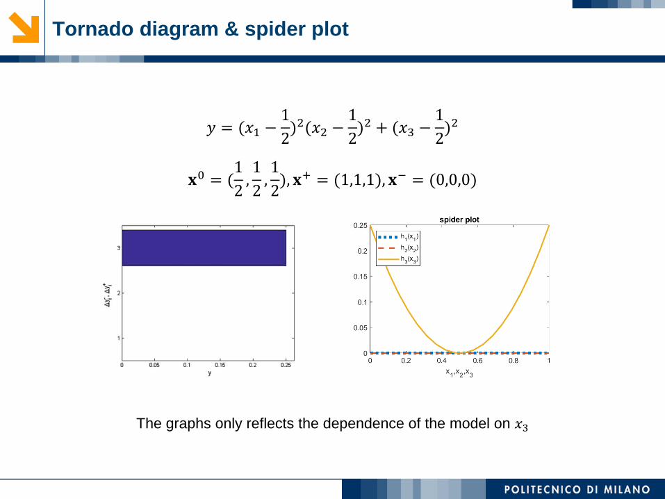
Tornado diagram & spider plot
The graphs only reflects the dependence of the model on 𝑥3
𝑦 = (𝑥1 −1
2)2(𝑥2 −
1
2)2 + (𝑥3 −
1
2)2
𝐱0 = (1
2,1
2,1
2), 𝐱+ = (1,1,1), 𝐱− = (0,0,0)
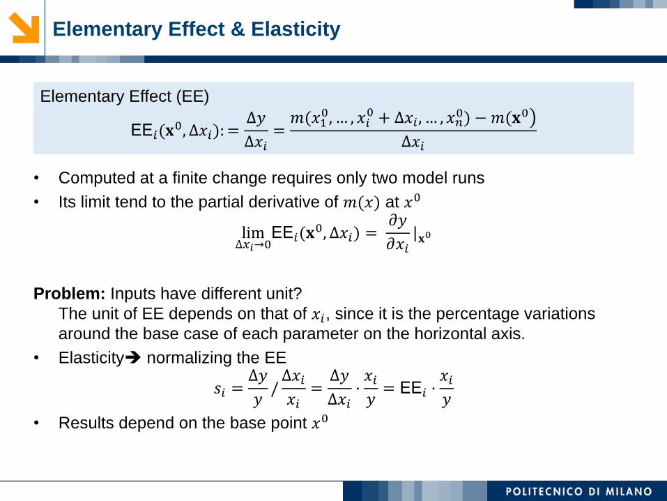
• Computed at a finite change requires only two model runs
• Its limit tend to the partial derivative of 𝑚(𝑥) at 𝑥0
lim∆𝑥𝑖→0
EE𝑖(𝐱0, ∆𝑥𝑖) =
𝜕𝑦
𝜕𝑥𝑖|𝐱0
Elementary Effect & Elasticity
Problem: Inputs have different unit?
The unit of EE depends on that of 𝑥𝑖, since it is the percentage variations
around the base case of each parameter on the horizontal axis.
• Elasticity➔ normalizing the EE
𝑠𝑖 =∆𝑦
𝑦/∆𝑥𝑖𝑥𝑖
=∆𝑦
∆𝑥𝑖·𝑥𝑖𝑦= EE𝑖 ·
𝑥𝑖𝑦
• Results depend on the base point 𝑥0
Elementary Effect (EE)
EE𝑖(𝐱0, ∆𝑥𝑖): =
∆𝑦
∆𝑥𝑖=
൯𝑚(𝑥10, … , 𝑥𝑖
0 + ∆𝑥𝑖 , … , 𝑥𝑛0) − 𝑚(𝐱0
∆𝑥𝑖

Idea of Morris method:
Generalize EE approach by varying the base point over the support of X and
averaging the results
EE & Morris’ method
Assume that the inputs are independent uniformly distributed in
0,1 𝑛, i.e. 𝑋𝑖 ~𝑖.𝑖.𝑑
𝑈 0,1
1. Define a grid of equally spaced (𝑝 + 1) points in each
dimension:
grid𝑖 = {0,1
𝑝,2
𝑝, … , 1}, 𝑖 = 1…𝑛,Grid = grid1 ⊗⋯⊗ grid𝑛
2. Select randomly 𝑁 different points {𝐱1, … , 𝐱𝑗 , … , 𝐱𝑁}
in the grid, and compute the EEijin each point and each
dimension.
𝐱𝑗
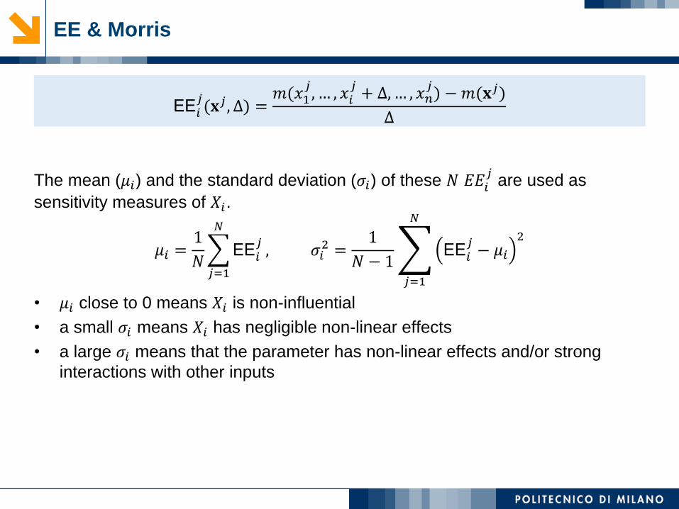
The mean (𝜇𝑖) and the standard deviation (𝜎𝑖) of these 𝑁 𝐸𝐸𝑖𝑗
are used as
sensitivity measures of 𝑋𝑖.
𝜇𝑖 =1
𝑁
𝑗=1
𝑁
EE𝑖𝑗, 𝜎𝑖
2 =1
𝑁 − 1
𝑗=1
𝑁
EE𝑖𝑗− 𝜇𝑖
2
• 𝜇𝑖 close to 0 means 𝑋𝑖 is non-influential
• a small 𝜎𝑖 means 𝑋𝑖 has negligible non-linear effects
• a large 𝜎𝑖 means that the parameter has non-linear effects and/or strong
interactions with other inputs
EE & Morris
EE𝑖𝑗(𝐱𝑗 , ∆) =
𝑚(𝑥1𝑗, … , 𝑥𝑖
𝑗+ ∆,… , 𝑥𝑛
𝑗) − 𝑚(𝐱𝑗)
∆
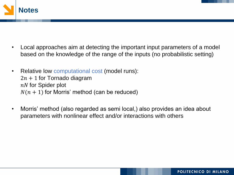
• Local approaches aim at detecting the important input parameters of a model
based on the knowledge of the range of the inputs (no probabilistic setting)
• Relative low computational cost (model runs):
2𝑛 + 1 for Tornado diagram
𝑛𝑁 for Spider plot
𝑁(𝑛 + 1) for Morris’ method (can be reduced)
• Morris’ method (also regarded as semi local,) also provides an idea about
parameters with nonlinear effect and/or interactions with others
Notes

GLOBAL APPROACHES
• Discrete:
Event and probability tree
Method of Discrete Probabilities
• Continuous:
Method of moments
Regression-based method
Distribution-based method

• Inputs and outputs are random variables: 𝑿, 𝑌
• Focus on determining the influence of inputs to the output uncertainty
distribution 𝑓𝒀(𝒚)
• 𝑓𝒀(𝒚) contains all relevant information on the uncertainty of the model
response regardless the values of the input
Global approaches
Global vs Local
• Global approaches account for the whole input variability range
Local approaches account for small variations around nominal values
• Global approaches account for interactions between the inputs
Local approaches consider variations of one input at a time
Better results at a higher computational expense
Discrete global approaches:
Event & probability tree (1)
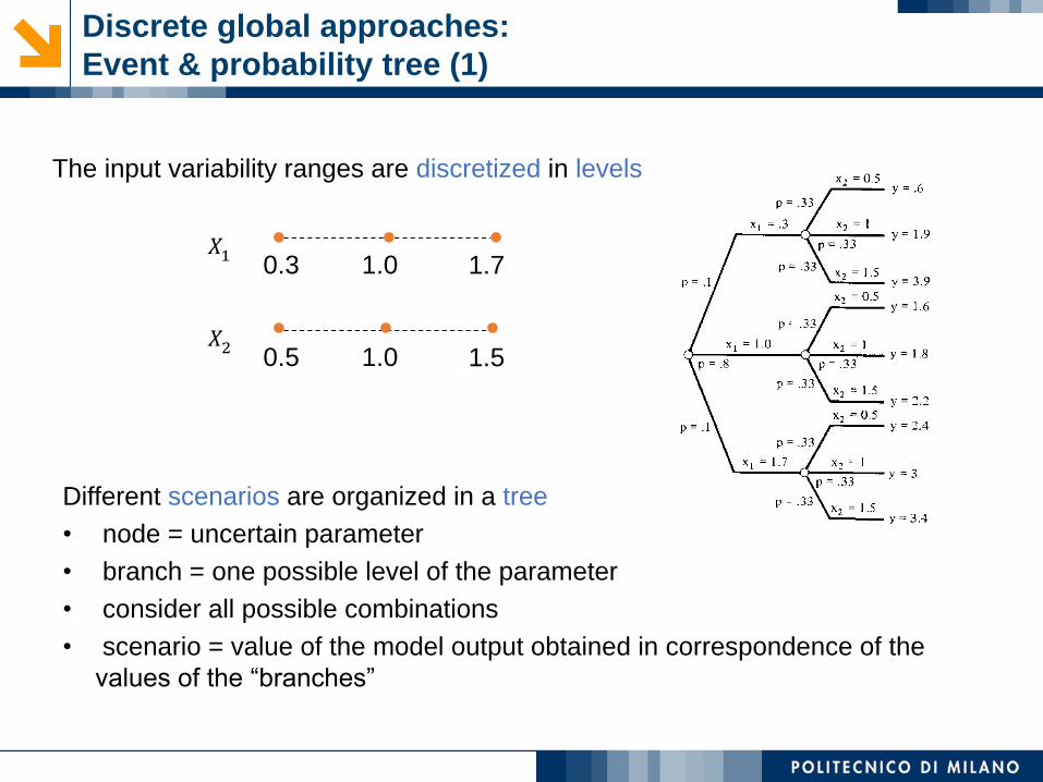
The input variability ranges are discretized in levels
Different scenarios are organized in a tree
• node = uncertain parameter
• branch = one possible level of the parameter
• consider all possible combinations
• scenario = value of the model output obtained in correspondence of the
values of the “branches”
𝑋10.3 1.71.0
𝑋20.5 1.51.0

• Assign discrete probabilities to the branches
o if discrete probability distributions → straightforward
o if continuous probability distributions → discretize
o probabilities of the branches are conditional on the values of the
“previous” branches
• Evaluate the probability of the scenarios y (product of conditional
probabilities)
Uncertainty
Propagation
Discrete global approaches:
Event & probability tree (2)

Discrete global approaches:
Event & probability tree (3)
• Extract sensitivity information (see sensitivity on the nominal range)
Sensitivity
Analysis
• It considers interactions between the inputs
• Problem: combinatorial explosion!
(𝑛 inputs, 𝑘 levels → 𝑘𝑛 combinations)
• To reduce computational cost ➔ discrete probability method
𝑦 = 𝑚(𝑥1, 𝑥2)
𝑥1
𝑥2 = 0.5
𝑥2 = 1
𝑥2 = 1.5
0.3 1.71.0
Discrete global approaches:
Discrete probability method (1)
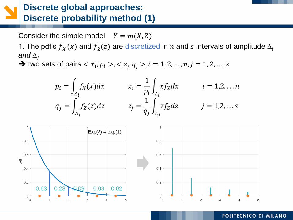
Consider the simple model 𝑌 = 𝑚(𝑋, 𝑍)
1. The pdf’s 𝑓𝑋 (𝑥) and 𝑓𝑍(𝑧) are discretized in 𝑛 and 𝑠 intervals of amplitude 𝑖and 𝑗➔ two sets of pairs < 𝑥𝑖 , 𝑝𝑖 >,< 𝑧𝑗, 𝑞𝑗 >, 𝑖 = 1, 2, … , 𝑛, 𝑗 = 1, 2, … , 𝑠
𝑝𝑖 = න𝛥𝑖
𝑓𝑋(𝑥)𝑑𝑥 𝑥𝑖 =1
𝑝𝑖න𝛥𝑖
𝑥𝑓𝑋𝑑𝑥 𝑖 = 1,2, . . . 𝑛
𝑞𝑗 = න𝛥𝑗
𝑓𝑍(𝑧)𝑑𝑧 𝑧𝑗 =1
𝑞𝑗න𝛥𝑗
𝑧𝑓𝑍𝑑𝑧 𝑗 = 1,2, . . . 𝑠
Exp(λ) = exp(1)
0.63 0.23 0.09 0.03 0.02
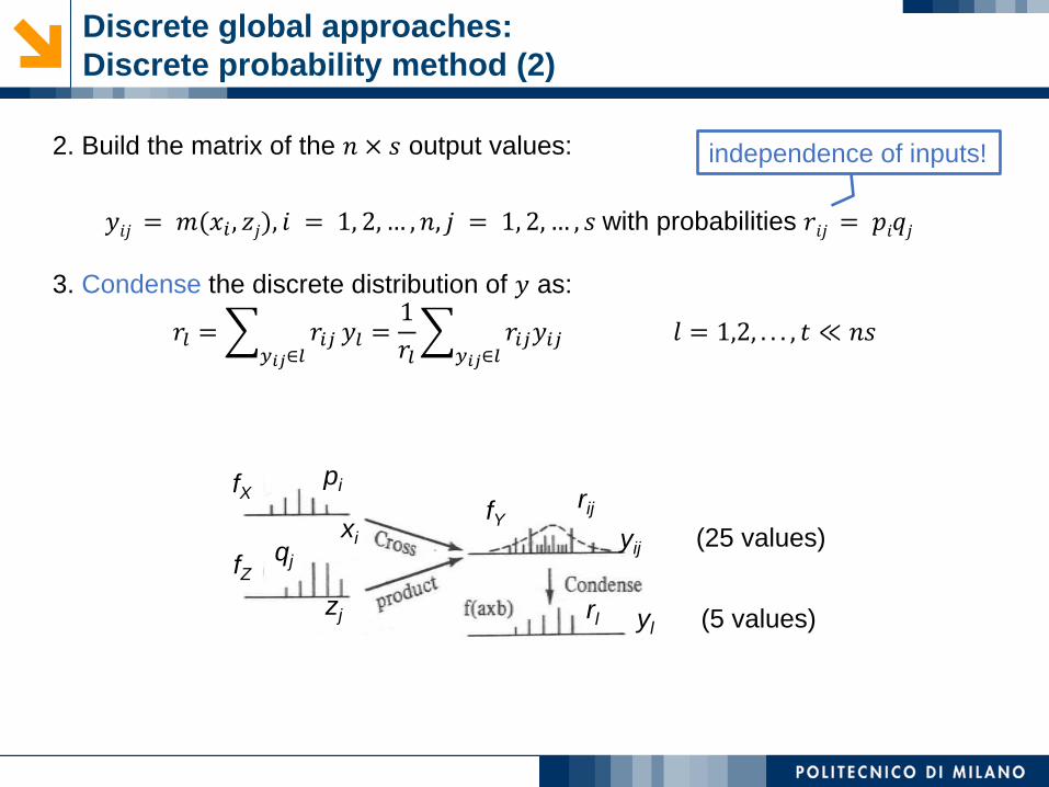
2. Build the matrix of the 𝑛 × 𝑠 output values:
𝑦𝑖𝑗 = 𝑚(𝑥𝑖 , 𝑧𝑗), 𝑖 = 1, 2, … , 𝑛, 𝑗 = 1, 2, … , 𝑠 with probabilities 𝑟𝑖𝑗 = 𝑝𝑖𝑞𝑗
3. Condense the discrete distribution of 𝑦 as:
𝑟𝑙 =𝑦𝑖𝑗∈𝑙
𝑟𝑖𝑗 𝑦𝑙 =1
𝑟𝑙
𝑦𝑖𝑗∈𝑙𝑟𝑖𝑗𝑦𝑖𝑗 𝑙 = 1,2, . . . , 𝑡 ≪ 𝑛𝑠
Discrete global approaches:
Discrete probability method (2)
independence of inputs!
fX
fZ
rij
yijxi
zj
pi
qj
fY
rl yl
(25 values)
(5 values)
Discrete global approaches:
Discrete probability method (3)
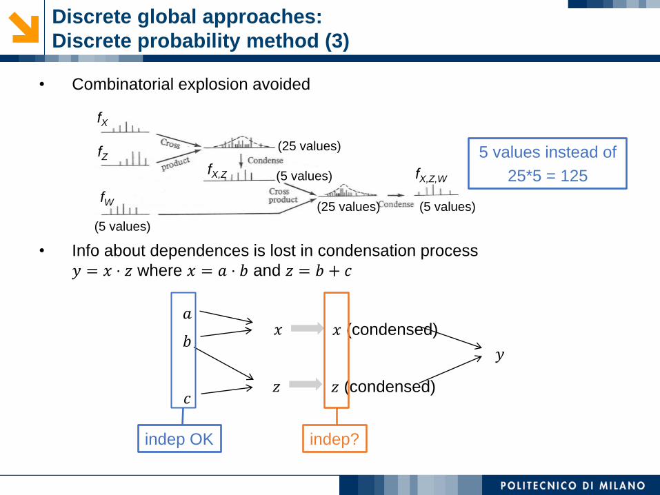
• Combinatorial explosion avoided
• Info about dependences is lost in condensation process
𝑦 = 𝑥 ⋅ 𝑧 where 𝑥 = 𝑎 ⋅ 𝑏 and 𝑧 = 𝑏 + 𝑐
fX
fZ
fW
fX,Z fX,Z,W
(25 values)
(5 values)
(5 values)
(25 values) (5 values)
5 values instead of
25*5 = 125
𝑎
𝑏
𝑐
𝑥
𝑧
𝑥 (condensed)
𝑧 (condensed)
𝑦
indep OK indep?

GLOBAL APPROACHES
• Discrete:
Event and probability tree
Method of Discrete Probabilities
• Continuous:
Method of moments
Regression-based method
Distribution-based method
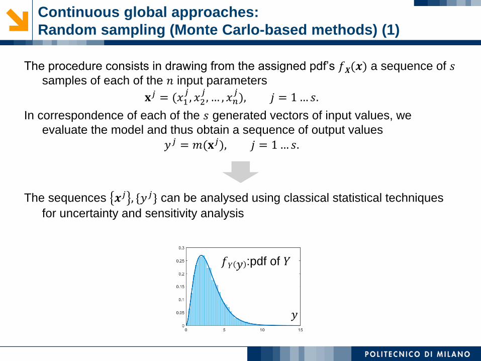
The procedure consists in drawing from the assigned pdf’s 𝑓𝑿(𝒙) a sequence of 𝑠samples of each of the 𝑛 input parameters
𝐱𝑗 = (𝑥1𝑗, 𝑥2
𝑗, … , 𝑥𝑛
𝑗), 𝑗 = 1…𝑠.
In correspondence of each of the 𝑠 generated vectors of input values, we
evaluate the model and thus obtain a sequence of output values
𝑦𝑗 = 𝑚(𝐱𝑗), 𝑗 = 1…𝑠.
The sequences 𝒙𝑗 , {𝑦𝑗} can be analysed using classical statistical techniques
for uncertainty and sensitivity analysis
Continuous global approaches:
Random sampling (Monte Carlo-based methods) (1)
𝑦
𝑓𝑌 𝑦 :pdf of 𝑌
• It covers the space of the input parameters by random sampling from the
corresponding probability distributions
• It provides a direct estimation of the output uncertainty via the corresponding
distribution 𝑓𝑌(𝑦)
• It is an approximated method, but its accuracy can be assessed and improved
by increasing the sample size s.
e.g. the RMSE of approximating mean using MC method is O s−1/2
Continuous global approaches:
Random sampling (Monte Carlo-based methods) (2)
Global approaches:
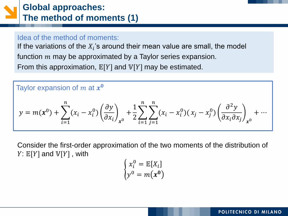
The method of moments (1)
Consider the first-order approximation of the two moments of the distribution of
𝑌: 𝔼[𝑌] and 𝕍[𝑌] , with
൝𝑥𝑖0 = 𝔼 𝑋𝑖
𝑦0 = 𝑚 𝒙𝟎
Idea of the method of moments:
If the variations of the 𝑋𝑖 ’s around their mean value are small, the model
function 𝑚 may be approximated by a Taylor series expansion.
From this approximation, 𝔼[𝑌] and 𝕍[𝑌] may be estimated.
Taylor expansion of 𝑚 at 𝒙𝟎
𝑦 = 𝑚(𝒙0) +
𝑖=1
𝑛
(𝑥𝑖 − 𝑥𝑖0)
𝜕𝑦
𝜕𝑥𝑖 𝒙0+1
2
𝑖=1
𝑛
𝑗=1
𝑛
(𝑥𝑖 − 𝑥𝑖0)( 𝑥𝑗 − 𝑥𝑗
0)𝜕2𝑦
𝜕𝑥𝑖𝜕𝑥𝑗 𝒙0+⋯
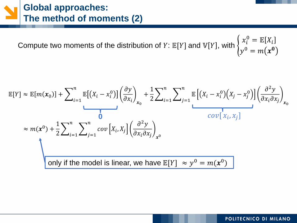
Global approaches:
The method of moments (2)
Compute two moments of the distribution of 𝑌: 𝔼[𝑌] and 𝕍 𝑌 , with ൝𝑥𝑖0 = 𝔼 𝑋𝑖
𝑦0 = 𝑚 𝒙𝟎
𝔼[𝑌] ≈ 𝔼 𝑚 𝒙0 +𝑖=1
𝑛
𝔼 𝑋𝑖 − 𝑥𝑖0 𝜕𝑦
𝜕𝑥𝑖 𝒙0
+1
2
𝑖=1
𝑛
𝑗=1
𝑛
𝔼 𝑋𝑖 − 𝑥𝑖0 𝑋𝑗 − 𝑥𝑗
0 𝜕2𝑦
𝜕𝑥𝑖𝜕𝑥𝑗 𝒙0
0 𝑐𝑜𝑣[ 𝑥𝑖 , 𝑥𝑗]
≈ 𝑚(𝒙0) +1
2
𝑖=1
𝑛
𝑗=1
𝑛
ቃ𝑐𝑜𝑣 ቂ𝑋𝑖 , 𝑋𝑗𝜕2𝑦
𝜕𝑥𝑖𝜕𝑥𝑗 𝒙0
only if the model is linear, we have 𝔼[𝑌] ≈ 𝑦0 = 𝑚(𝒙0)
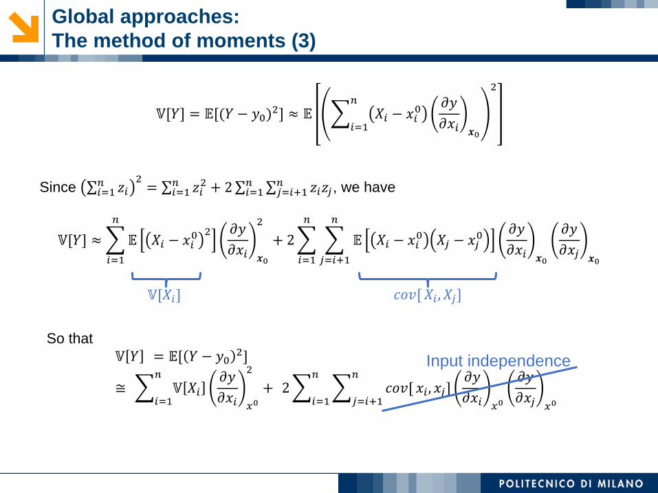
Global approaches:
The method of moments (3)
𝕍[𝑌] = 𝔼[(𝑌 − 𝑦0)2] ≈ 𝔼
𝑖=1
𝑛
𝑋𝑖 − 𝑥𝑖0 𝜕𝑦
𝜕𝑥𝑖 𝒙0
2
Since σ𝑖=1𝑛 𝑧𝑖
2= σ𝑖=1
𝑛 𝑧𝑖2 + 2σ𝑖=1
𝑛 σ𝑗=𝑖+1𝑛 𝑧𝑖𝑧𝑗, we have
𝕍[𝑌] ≈
𝑖=1
𝑛
𝔼 𝑋𝑖 − 𝑥𝑖0 2 𝜕𝑦
𝜕𝑥𝑖 𝒙0
2
+ 2
𝑖=1
𝑛
𝑗=𝑖+1
𝑛
𝔼 𝑋𝑖 − 𝑥𝑖0 𝑋𝑗 − 𝑥𝑗
0 𝜕𝑦
𝜕𝑥𝑖 𝒙0
𝜕𝑦
𝜕𝑥𝑗 𝒙0
𝕍[𝑋𝑖] 𝑐𝑜𝑣[ 𝑋𝑖 , 𝑋𝑗]
So that
𝕍 𝑌 = 𝔼[ 𝑌 − 𝑦02]
≅ 𝑖=1
𝑛
𝕍 𝑋𝑖𝜕𝑦
𝜕𝑥𝑖 𝑥0
2
+ 2𝑖=1
𝑛
𝑗=𝑖+1
𝑛
𝑐𝑜𝑣[ 𝑥𝑖 , 𝑥𝑗]𝜕𝑦
𝜕𝑥𝑖 𝑥0
𝜕𝑦
𝜕𝑥𝑗 𝑥0
Input independence
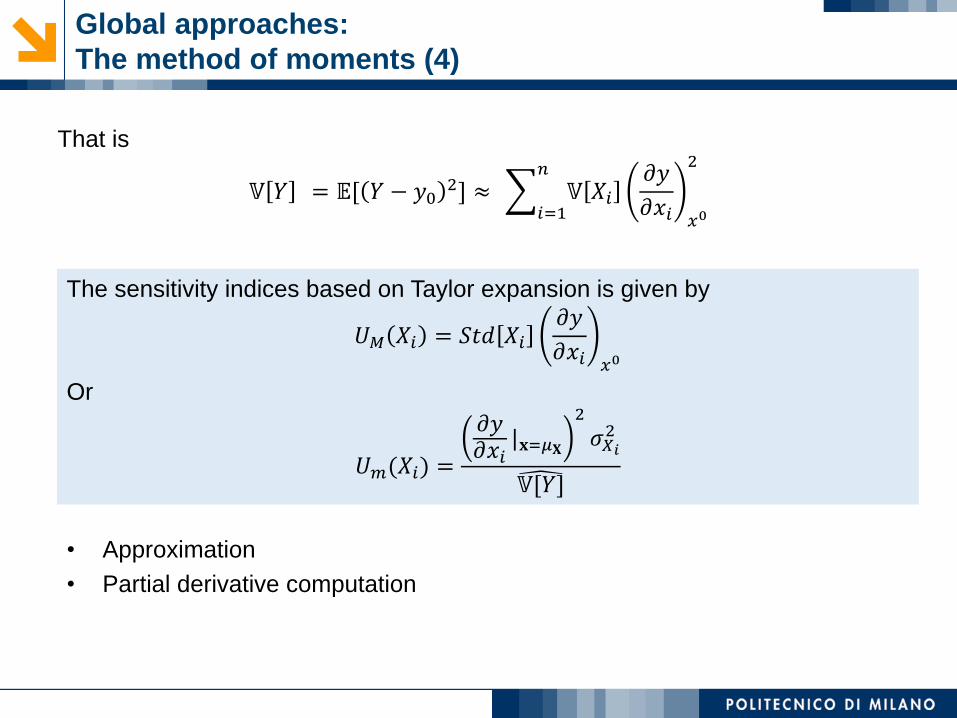
Global approaches:
The method of moments (4)
• Approximation
• Partial derivative computation
That is
𝕍 𝑌 = 𝔼[ 𝑌 − 𝑦02] ≈
𝑖=1
𝑛
𝕍 𝑋𝑖𝜕𝑦
𝜕𝑥𝑖 𝑥0
2
The sensitivity indices based on Taylor expansion is given by
𝑈𝑀 𝑋𝑖 = 𝑆𝑡𝑑 𝑋𝑖𝜕𝑦
𝜕𝑥𝑖 𝑥0
Or
𝑈𝑚(𝑋𝑖) =
𝜕𝑦𝜕𝑥𝑖
|𝐱=𝜇𝐗
2
𝜎𝑋𝑖2
𝕍[𝑌]
Continuous global approaches:
Pearson’s Input/output correlation coefficients, 1880s
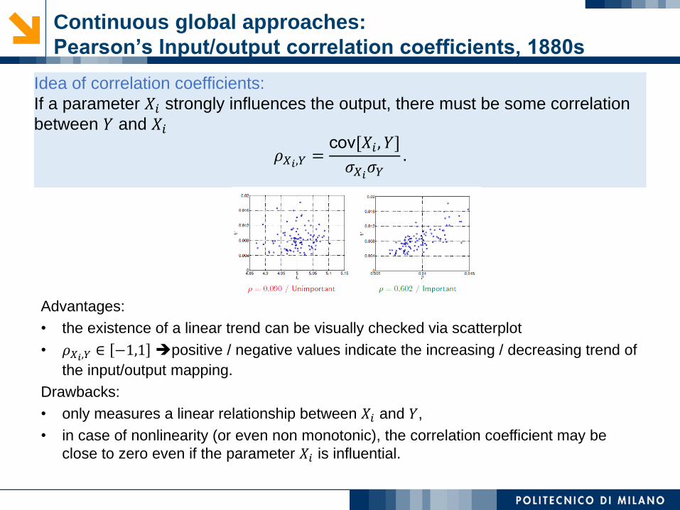
Idea of correlation coefficients:
If a parameter 𝑋𝑖 strongly influences the output, there must be some correlation
between 𝑌 and 𝑋𝑖
𝜌𝑋𝑖,𝑌 =cov[𝑋𝑖 , 𝑌]
𝜎𝑋𝑖𝜎𝑌.
Advantages:
• the existence of a linear trend can be visually checked via scatterplot
• 𝜌𝑋𝑖,𝑌 ∈ −1,1 ➔positive / negative values indicate the increasing / decreasing trend of
the input/output mapping.
Drawbacks:
• only measures a linear relationship between 𝑋𝑖 and 𝑌,
• in case of nonlinearity (or even non monotonic), the correlation coefficient may be
close to zero even if the parameter 𝑋𝑖 is influential.
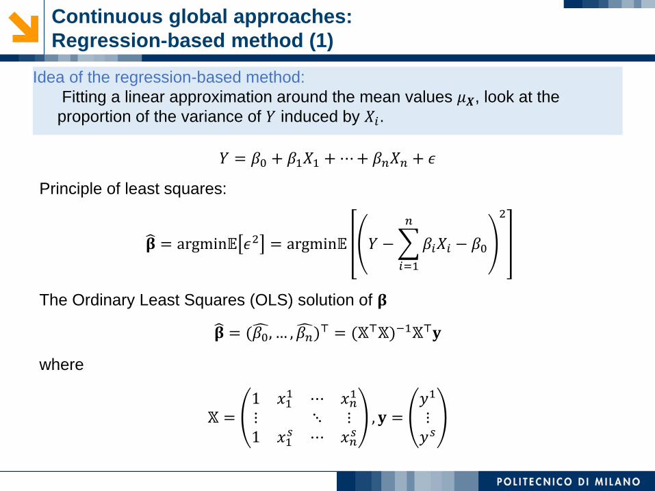
Idea of the regression-based method:
Fitting a linear approximation around the mean values 𝜇𝑿, look at the
proportion of the variance of 𝑌 induced by 𝑋𝑖.
Continuous global approaches:
Regression-based method (1)
𝑌 = 𝛽0 + 𝛽1𝑋1 +⋯+ 𝛽𝑛𝑋𝑛 + 𝜖
Principle of least squares:
𝛃 = argmin𝔼 𝜖2 = argmin𝔼 𝑌 −
𝑖=1
𝑛
𝛽𝑖𝑋𝑖 − 𝛽0
2
The Ordinary Least Squares (OLS) solution of 𝛃
𝛃 = (𝛽0, … , 𝛽𝑛)⊤ = (𝕏⊤𝕏)−1𝕏⊤𝐲
where
𝕏 =1 𝑥1
1 ⋯ 𝑥𝑛1
⋮ ⋱ ⋮1 𝑥1
𝑠 ⋯ 𝑥𝑛𝑠
, 𝐲 =𝑦1
⋮𝑦𝑠

The Standard Regression Coefficients SRC𝑖 associated with 𝑋𝑖 is given as:
SRC𝑖: = 𝛽𝑖𝜎𝑋𝑖𝜎𝑌
Continuous global approaches:
Regression-based method (2)
Under assumptions
• the input variables are independent,
• ϵ is independent of the inputs,
the variance decomposition of 𝑌 is given by
𝕍[𝑌] =
𝑖=1
𝑛
𝛽𝑖2𝕍[𝑋𝑖] + 𝜎𝜖
2.
Thus, 𝛽𝑖2𝕍[𝑋𝑖] is the proportion of the variance of 𝑌 induced by 𝑋𝑖.
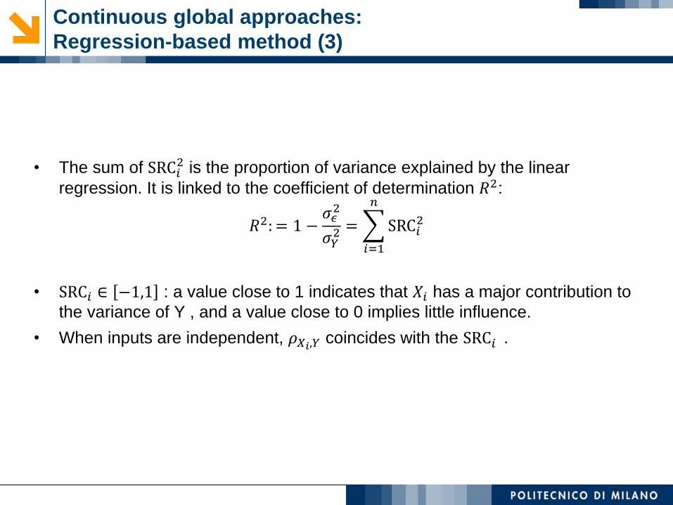
• The sum of SRC𝑖2 is the proportion of variance explained by the linear
regression. It is linked to the coefficient of determination 𝑅2:
𝑅2: = 1 −𝜎𝜖2
𝜎𝑌2 =
𝑖=1
𝑛
SRC𝑖2
• SRC𝑖 ∈ −1,1 : a value close to 1 indicates that 𝑋𝑖 has a major contribution to
the variance of Y , and a value close to 0 implies little influence.
• When inputs are independent, 𝜌𝑋𝑖,𝑌 coincides with the SRC𝑖 .
Continuous global approaches:
Regression-based method (3)
Notes
• When the model is linear or accurately approximated by a linear model:
▪ Importance measures based on Taylor series expansion
▪ Input/output correlation coefficients
▪ Standard regression coefficients
• In case of non linear, yet monotonic models the rank transform shall be used:
• Input/output rank correlation coefficients
• Standard Rank Regression Coefficients (SRRC)
• For more general situations, one may consider distribution-based methods.

GLOBAL APPROACHES
• Discrete:
Event and probability tree
Method of Discrete Probabilities
• Continuous:
Method of moments
Regression-based method
Distribution-based method
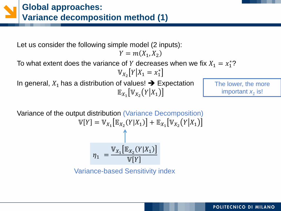
Let us consider the following simple model (2 inputs):
𝑌 = 𝑚 𝑋1, 𝑋2To what extent does the variance of 𝑌 decreases when we fix 𝑋1 = 𝑥1
∗?
𝕍𝑋2 𝑌ห𝑋1 = 𝑥1∗
In general, 𝑋1 has a distribution of values! ➔ Expectation
𝔼𝑋1 𝕍𝑋2 𝑌ห𝑋1
Variance of the output distribution (Variance Decomposition)
𝕍 𝑌 = 𝕍𝑋1 𝔼𝑋2 𝑌|𝑋1 + 𝔼𝑋1 𝕍𝑋2 𝑌ห𝑋1
The lower, the more
important x1 is!
𝜂1 =𝕍𝑋1 𝔼𝑋2 𝑌|𝑋1
𝕍 𝑌
Variance-based Sensitivity index
Global approaches:
Variance decomposition method (1)
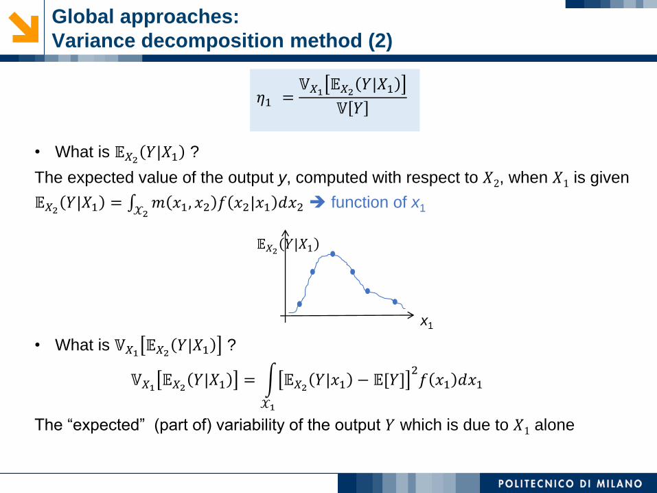
• What is 𝔼𝑋2 𝑌|𝑋1 ?
The expected value of the output y, computed with respect to 𝑋2, when 𝑋1 is given
𝔼𝑋2 𝑌|𝑋1 = 𝒳2𝑚 𝑥1, 𝑥2 𝑓 𝑥2|𝑥1 𝑑𝑥2 ➔ function of x1
𝔼𝑋2 𝑌|𝑋1
x1
• What is 𝕍𝑋1 𝔼𝑋2 𝑌|𝑋1 ?
𝕍𝑋1 𝔼𝑋2 𝑌|𝑋1 = න
𝒳1
𝔼𝑋2 𝑌|𝑥1 − 𝔼[𝑌]2𝑓 𝑥1 𝑑𝑥1
The “expected” (part of) variability of the output 𝑌 which is due to 𝑋1 alone
Global approaches:
Variance decomposition method (2)
𝜂1 =𝕍𝑋1 𝔼𝑋2 𝑌|𝑋1
𝕍 𝑌
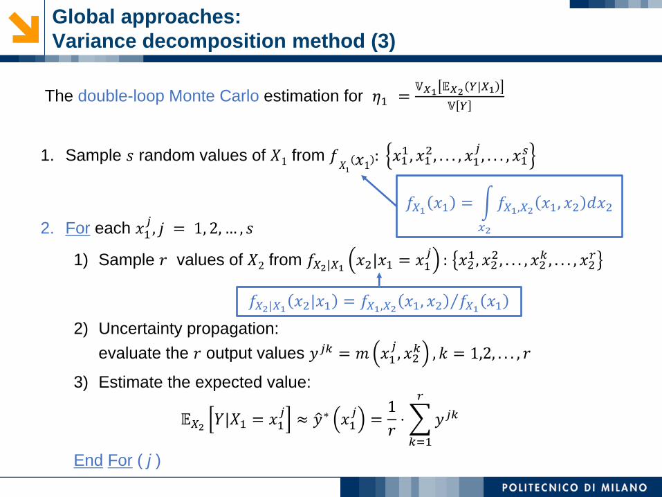
1. Sample 𝑠 random values of 𝑋1 from 𝑓𝑋1𝑥1 : 𝑥1
1, 𝑥12, . . . , 𝑥1
𝑗, . . . , 𝑥1
𝑠
2. For each 𝑥1𝑗, 𝑗 = 1, 2, … , 𝑠
1) Sample 𝑟 values of 𝑋2 from 𝑓𝑋2|𝑋1 𝑥2|𝑥1 = 𝑥1𝑗: 𝑥2
1, 𝑥22, . . . , 𝑥2
𝑘 , . . . , 𝑥2𝑟
2) Uncertainty propagation:
evaluate the 𝑟 output values 𝑦𝑗𝑘 = 𝑚 𝑥1𝑗, 𝑥2
𝑘 , 𝑘 = 1,2, . . . , 𝑟
3) Estimate the expected value:
𝔼𝑋2 𝑌|𝑋1 = 𝑥1𝑗≈ ො𝑦∗ 𝑥1
𝑗=1
𝑟⋅
𝑘=1
𝑟
𝑦𝑗𝑘
End For ( j )
The double-loop Monte Carlo estimation for 𝜂1 =𝕍𝑋1 𝔼𝑋2 𝑌|𝑋1
𝕍 𝑌
Global approaches:
Variance decomposition method (3)
𝑓𝑋1 𝑥1 = න
𝑥2
𝑓𝑋1,𝑋2 𝑥1, 𝑥2 𝑑𝑥2
𝑓𝑋2|𝑋1 𝑥2|𝑥1 = Τ𝑓𝑋1,𝑋2 𝑥1, 𝑥2 𝑓𝑋1 𝑥1
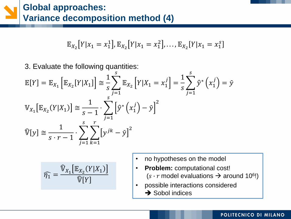
𝔼𝑋2 𝑌|𝑥1 = 𝑥11 , 𝔼𝑋2 𝑌|𝑥1 = 𝑥1
2 , . . . , 𝔼𝑋2 𝑌|𝑥1 = 𝑥1𝑠
3. Evaluate the following quantities:
𝔼 𝑌 = 𝔼𝑋1 𝔼𝑋2 𝑌|𝑋1 ≅1
𝑠
𝑗=1
𝑠
𝔼𝑋2 𝑌|𝑋1 = 𝑥1𝑗=1
𝑠
𝑗=1
𝑠
ො𝑦∗ 𝑥1𝑗= lj𝑦
𝕍𝑋1 𝔼𝑋2 𝑌|𝑋1 ≅1
𝑠 − 1⋅
𝑗=1
𝑠
ො𝑦∗ 𝑥1𝑗− lj𝑦
2
𝕍 𝑦 ≅1
𝑠 ⋅ 𝑟 − 1⋅
𝑗=1
𝑠
𝑘=1
𝑟
𝑦𝑗𝑘 − lj𝑦2
• no hypotheses on the model
• Problem: computational cost!
(𝑠 ∙ 𝑟 model evaluations → around 106!)
• possible interactions considered
➔ Sobol indices
Global approaches:
Variance decomposition method (4)
ෞ𝜂1 =𝕍𝑋1 𝔼𝑋2 𝑌|𝑋1
𝕍 𝑌
Contribution of 𝑋1 and 𝑋2(alone and interacting)
𝑋1 alone 𝑋2 alone
= only interaction!
Global approaches:
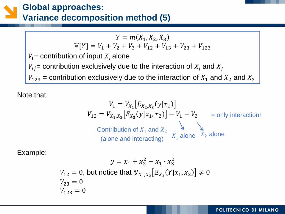
Variance decomposition method (5)
𝑌 = 𝑚 𝑋1, 𝑋2, 𝑋3𝕍[𝑌] = 𝑉1 + 𝑉2 + 𝑉3 + 𝑉12 + 𝑉13 + 𝑉23 + 𝑉123
𝑉𝑖= contribution of input 𝑋𝑖 alone
𝑉𝑖𝑗= contribution exclusively due to the interaction of 𝑋𝑖 and 𝑋𝑗
𝑉123 = contribution exclusively due to the interaction of 𝑋1 and 𝑋2 and 𝑋3
Note that:
𝑉1 = 𝑉𝑋1 𝐸𝑋2,𝑋3 𝑦|𝑥1𝑉12 = 𝑉𝑋1,𝑋2 𝐸𝑋3 𝑦|𝑥1, 𝑥2 − 𝑉1 − 𝑉2
Example:
𝑦 = 𝑥1 + 𝑥22 + 𝑥1 ⋅ 𝑥3
2
𝑉12 = 0, but notice that 𝕍𝑋1,𝑋2 𝔼𝑋3 𝑌|𝑥1, 𝑥2 ≠ 0
𝑉23 = 0𝑉123 = 0
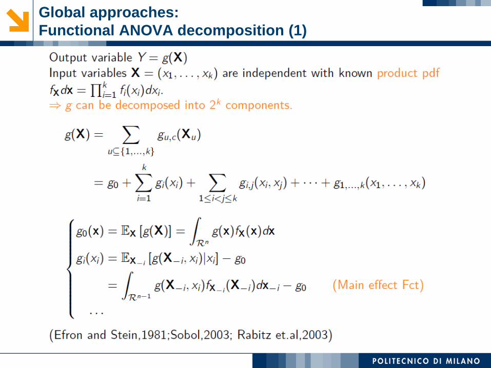
Global approaches:
Functional ANOVA decomposition (1)

Global approaches:
Functional ANOVA decomposition (2)
• The index 𝑆𝑖 corresponds to the fraction of 𝕍[𝑌] associated with the individual
contribution of 𝑋𝑖.
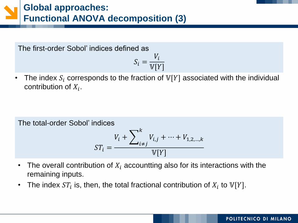
Global approaches:
Functional ANOVA decomposition (3)
The first-order Sobol’ indices defined as
𝑆𝑖 =𝑉𝑖𝕍[𝑌]
• The overall contribution of 𝑋𝑖 accountting also for its interactions with the
remaining inputs.
• The index 𝑆𝑇𝑖 is, then, the total fractional contribution of 𝑋𝑖 to 𝕍[𝑌].
The total-order Sobol’ indices
𝑆𝑇𝑖 =
𝑉𝑖 +𝑖≠𝑗
𝑘
𝑉𝑖,𝑗 +⋯+ 𝑉1,2,…,𝑘
𝕍[𝑌]
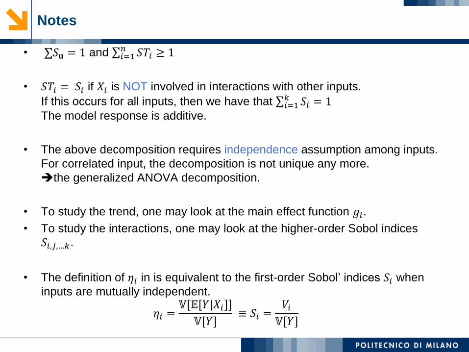
• σ𝑆𝐮 = 1 and σ𝑖=1𝑛 𝑆𝑇𝑖 ≥ 1
• 𝑆𝑇𝑖 = 𝑆𝑖 if 𝑋𝑖 is NOT involved in interactions with other inputs.
If this occurs for all inputs, then we have that σ𝑖=1𝑘 𝑆𝑖 = 1
The model response is additive.
• The above decomposition requires independence assumption among inputs.
For correlated input, the decomposition is not unique any more.
➔the generalized ANOVA decomposition.
• To study the trend, one may look at the main effect function 𝑔𝑖.
• To study the interactions, one may look at the higher-order Sobol indices
𝑆𝑖,𝑗,…𝑘.
• The definition of 𝜂𝑖 in is equivalent to the first-order Sobol’ indices 𝑆𝑖 when
inputs are mutually independent.
𝜂𝑖 =𝕍[𝔼[𝑌|𝑋𝑖]]
𝕍[𝑌]≡ 𝑆𝑖 =
𝑉𝑖𝕍[𝑌]
Notes
Global approaches:
Moment-independent sensitivity measures (1)
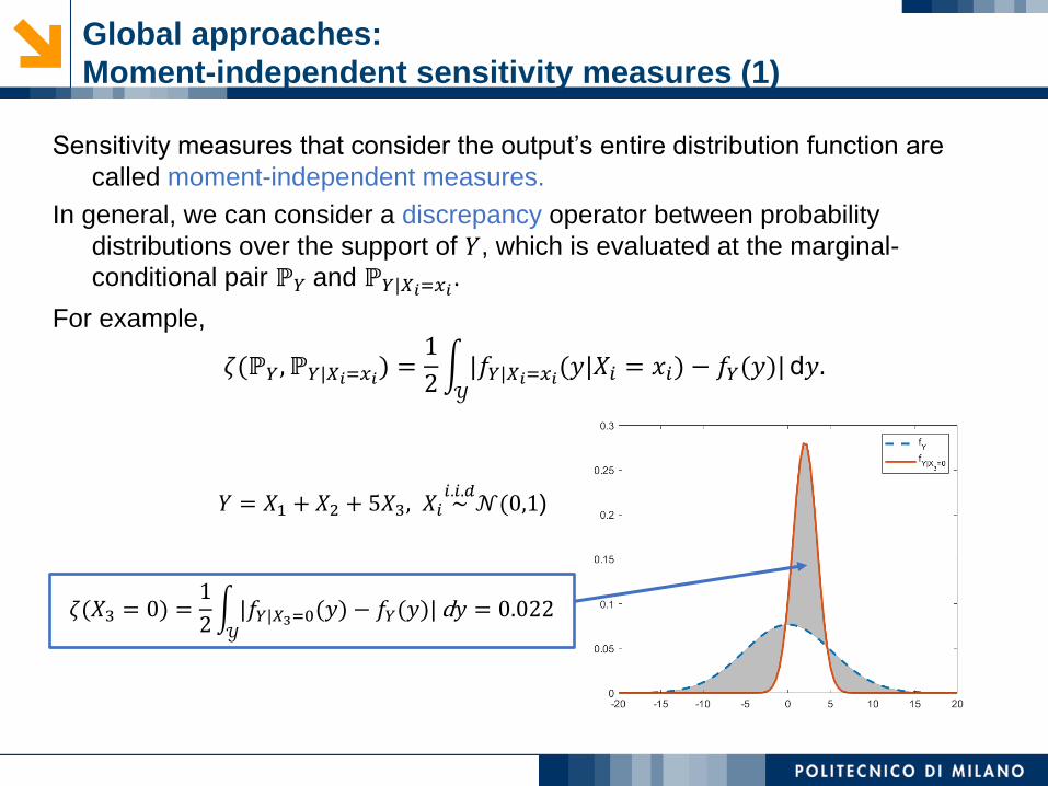
Sensitivity measures that consider the output’s entire distribution function are
called moment-independent measures.
In general, we can consider a discrepancy operator between probability
distributions over the support of 𝑌, which is evaluated at the marginal-
conditional pair ℙ𝑌 and ℙ𝑌|𝑋𝑖=𝑥𝑖.
For example,
𝜁(ℙ𝑌, ℙ𝑌|𝑋𝑖=𝑥𝑖) =1
2න𝒴
|𝑓𝑌|𝑋𝑖=𝑥𝑖(𝑦|𝑋𝑖 = 𝑥𝑖) − 𝑓𝑌(𝑦)| d𝑦.
𝑌 = 𝑋1 + 𝑋2 + 5𝑋3, 𝑋𝑖 ~𝑖.𝑖.𝑑
𝒩(0,1)
𝜁(𝑋3 = 0) =1
2න𝒴
|𝑓𝑌|𝑋3=0(𝑦) − 𝑓𝑌(𝑦)| d𝑦 = 0.022
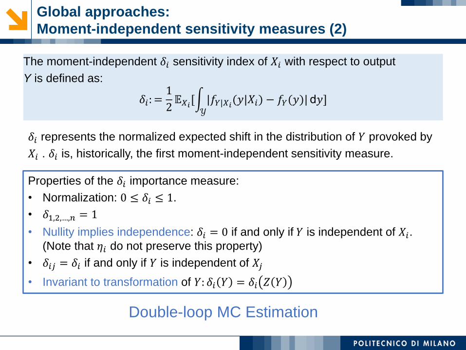
The moment-independent 𝛿𝑖 sensitivity index of 𝑋𝑖 with respect to output
Y is defined as:
𝛿𝑖: =1
2𝔼𝑋𝑖[න
𝒴
|𝑓𝑌|𝑋𝑖(𝑦|𝑋𝑖) − 𝑓𝑌(𝑦)| d𝑦]
Global approaches:
Moment-independent sensitivity measures (2)
Double-loop MC Estimation
𝛿𝑖 represents the normalized expected shift in the distribution of 𝑌 provoked by
𝑋𝑖 . 𝛿𝑖 is, historically, the first moment-independent sensitivity measure.
Properties of the 𝛿𝑖 importance measure:
• Normalization: 0 ≤ 𝛿𝑖 ≤ 1.
• 𝛿1,2,…,𝑛 = 1
• Nullity implies independence: 𝛿𝑖 = 0 if and only if 𝑌 is independent of 𝑋𝑖. (Note that 𝜂𝑖 do not preserve this property)
• 𝛿𝑖𝑗 = 𝛿𝑖 if and only if 𝑌 is independent of 𝑋𝑗
• Invariant to transformation of 𝑌: 𝛿𝑖 𝑌 = 𝛿𝑖 𝑍 𝑌
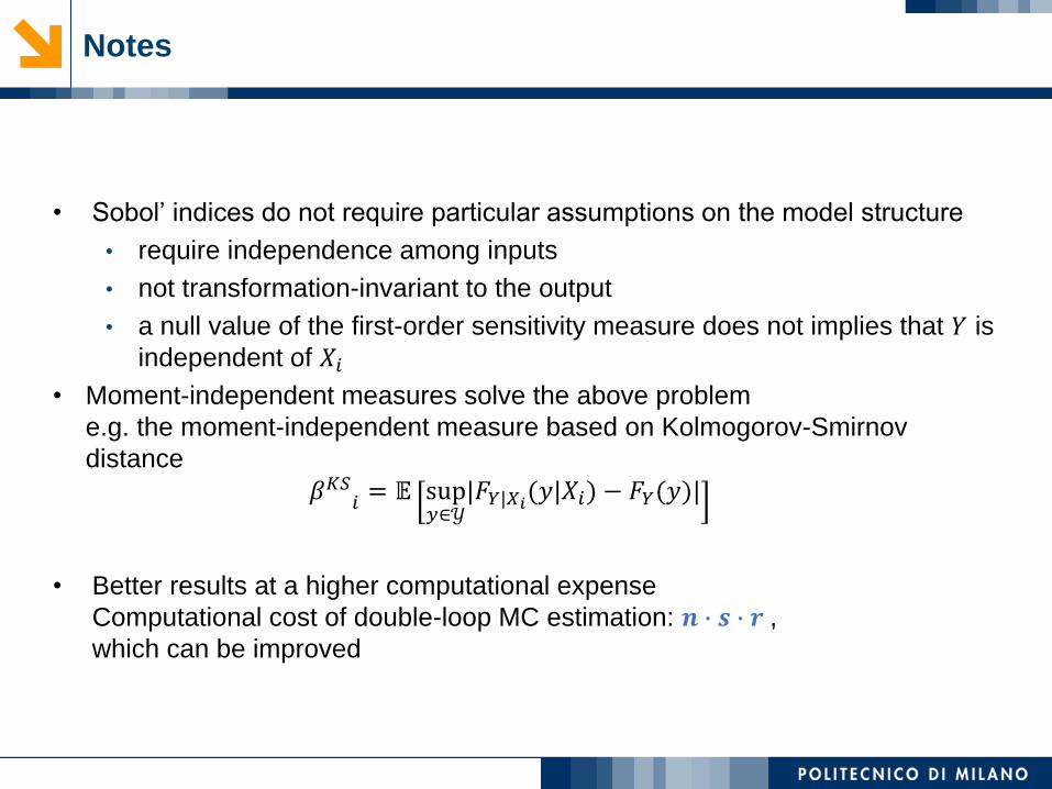
• Sobol’ indices do not require particular assumptions on the model structure
• require independence among inputs
• not transformation-invariant to the output
• a null value of the first-order sensitivity measure does not implies that 𝑌 is
independent of 𝑋𝑖• Moment-independent measures solve the above problem
e.g. the moment-independent measure based on Kolmogorov-Smirnov
distance
𝛽𝐾𝑆𝑖= 𝔼 sup
𝑦∈𝒴|𝐹𝑌|𝑋𝑖(𝑦|𝑋𝑖) − 𝐹𝑌(𝑦)|
• Better results at a higher computational expense
Computational cost of double-loop MC estimation: 𝒏 ∙ 𝒔 ∙ 𝒓 ,
which can be improved
Notes

MODEL (STRUCTURE)
UNCERTAINTY
• The alternative model approach
• The perturbative treatment of the reference model

Model (structure) uncertainty:
The alternative model approach
Consider a set of 𝑀 plausible models 𝑚𝑖, 𝑖 = 1,2, … ,𝑀 , each characterized by a
set of uncertain parameters 𝒂𝒊 with distribution (𝒂𝒊| 𝑚𝑖)
𝑦𝑖 𝐱, 𝐚𝑖 = 𝑚𝑖 𝐱, 𝐚𝑖
𝑦𝑖 𝐱 = න
𝐚𝑖
𝑚𝑖 𝐱, 𝐚𝑖 𝜋 𝐚𝑖|𝑚𝑖 𝑑𝐚𝑖
Model uncertainty quantified by a discrete probability distribution
𝑝(𝑚𝑖), 𝑖 = 1, 2, … ,𝑀
Output 𝑦 estimation ➔ total probability theorem
𝑦 𝐱 =
𝑖=1
𝑀
𝑝 𝑚𝑖 න
𝐚𝑖
𝑚𝑖 𝐱, 𝐚𝑖 𝜋 𝐚𝑖|𝑚𝑖 𝑑𝐚𝑖

Model (structure) uncertainty:
The perturbative treatment of the reference model
• One single model 𝑚∗ is considered, typically the most plausible, and a
perturbation is directly introduced in the model output
• The perturbation is a sort of error term with which one accounts for the
structural uncertainties due to the incomplete knowledge of the
phenomenon
• In practice, one adopts additional or multiplicative perturbative terms
𝑦 = 𝑚∗(𝒙, 𝒂∗) + 𝐷𝑎∗ 𝑦 = 𝑚∗ 𝒙, 𝒂∗ 𝐷𝑚
∗
• The perturbations 𝐷𝑎∗ and 𝐷𝑚
∗ are not exactly known, but they may be
described in terms of opportune probability distributions
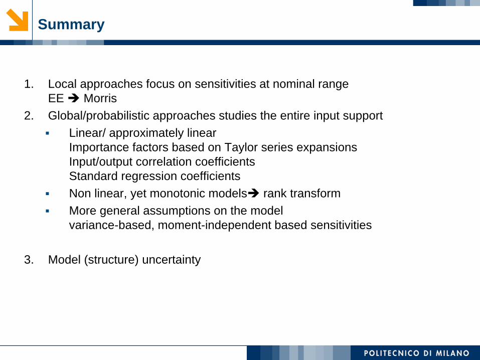
Summary
1. Local approaches focus on sensitivities at nominal range
EE ➔ Morris
2. Global/probabilistic approaches studies the entire input support
▪ Linear/ approximately linear
Importance factors based on Taylor series expansions
Input/output correlation coefficients
Standard regression coefficients
▪ Non linear, yet monotonic models➔ rank transform
▪ More general assumptions on the model
variance-based, moment-independent based sensitivities
3. Model (structure) uncertainty

QUESTIONS?
Xuefei Lu