Uncertainty and the Demand for Insurance(PRELIMINARY)

Amit GandhiUniversity of Pennsylvania and Airbnb

Anya SamekUniversity of California, San Diego

Ricardo Serrano-Padial∗

Drexel University

October 22, 2021

AbstractWe investigate the determinants of insurance demand under uncertainty about

underlying risks. We use demand elicitation surveys on a representative sample ofUS households in which we vary risks and the degree of uncertainty about them.We find that uncertainty in the form of compound and ambiguous risks can leadto large increases in individual demand for insurance. We also find that riskaversion and uncertainty aversion are negatively related in the population. Weshow that preferences that rely on expected utility for the evaluation of known(objective) risks cannot explain the data. In contrast, we prove that second-orderanticipated utility exhibiting probability weighting can rationalize the observedpatterns and be tractably estimated. Our preference estimates imply substantialoverweighting of small probabilities and underweighting of large probabilities. Wefind that preference heterogeneity is largely driven by substantial heterogeneityof probability weighting of known (objective) risks.

JEL classification: D12, D14, D81, G22, J33

Keywords : risk, uncertainty, ambiguity, insurance, compound risk, probability weight-ing, incentivized survey

∗Corresponding Author: Ricardo Serrano-Padial, email: rspadial@gmail.com. We thank DavidDillenberger, Ben Handel, Glenn Harrison, Shaowei Ke, Jay Lu, Adam Sanjurjo, Charlie Sprenger,Shoshana Vasserman and audiences at the NBER summer institute in IO, Alicante, Risk TheorySociety, CEAR Behavioral Insurance Workshop and the ASSA/Econometric Society winter meetingsfor helpful comments. This paper was funded as a pilot project as part of a Roybal grant awardedto the University of Southern California, entitled “Roybal Center for Health Decision Making andFinancial Independence in Old Age” (5P30AG024962-12). The project described in this paper relieson data from surveys administered by the Understanding America Study (UAS) which is maintainedby the Center for Economic and Social Research (CESR) at the University of Southern California.The opinions and conclusions expressed herein are solely those of the authors and do not representthe opinions or policy of any institution with which the authors are affiliated nor of USC, CESR orthe UAS.

1 Introduction

Insurance markets play a central role in the economy. In the United States, insurancepremiums amount to $1.2 trillion each year, or about 7% of gross domestic product.1

Arguably the most critical task faced by consumers in these markets is the assessmentof their underlying risks in the presence of uncertainty and complex information aboutthose risks. In this context, laboratory experiments using lottery choices have docu-mented that individuals are ambiguity averse and have difficulty reducing compoundlotteries (Halevy, 2007). This suggests that willingness-to-pay (WTP) for insuranceshould be higher under uncertainty than under known risks. That is, uncertainty averseconsumers would be willing to pay an “uncertainty premium” to obtain insurance, ontop of the risk premium associated with aversion to known risks.

However, while there is a growing literature on the estimation of risk preferencesfrom insurance data, little is known about the nature of uncertainty preferences in thepopulation and the overall impact of uncertainty on insurance demand. This paperaims to fill this gap by analyzing the demand for insurance under uncertainty and byestimating the distribution of uncertainty preferences in the population. We overcomethe inherent lack of observability of demand determinants using an incentivized surveyon a representative sample of the U.S. population that elicits individual demand underdifferent risk and uncertainty scenarios.

The paper makes three main contributions. First, we quantify the impact of uncer-tainty on insurance demand and document key empirical regularities of WTP for in-surance under uncertainty. Second, we theoretically identify conditions on uncertaintypreferences needed to explain these patterns and characterize a class of preferences thatcan rationalize the data. Finally, equipped with this characterization, we estimate thedistribution of uncertainty preferences in the population and examine the degree andsources of preference heterogeneity. We also show how to partially identify uncertaintypreferences and do welfare analysis using field data from insurance markets.

In our survey, over 4,000 individuals representative of the U.S. population are givenmonetary incentives to reveal their WTP to fully insure a hypothetical product that hasa known value. Respondents make a series of decisions in which we exogenously varyboth the risk probability that the product looses its value and the degree of uncertaintyabout the risk probability. We introduce uncertainty by making risk probability arandom variable, and either inform agents about its distribution (compound risks) or itspossible range of values (ambiguous risks). We elicit agents’ WTP under both known

1See https://www.iii.org/fact-statistic/facts-statistics-industry-overview.

1

risks, in which agents are given the actual risk probability, and unknown risks (wesplit the sample of respondents between compound and ambiguous risks). The surveyincludes rich sociodemographic information, including measures of financial literacyand cognitive ability.

Our data reveals several key patterns of demand behavior. First, uncertainty sig-nificantly increases individuals’ willingness to pay (WTP) for insurance. To measureits magnitude, we define the uncertainty premium as the difference in WTP between agiven unknown risk and the known risk whose probability equals the mean probabilityof the unknown risk. We observe uncertainty premia as high as 100% of the actuar-ially fair price of insurance, especially at low risk probabilities. Importantly, we findthat the uncertainty premium is negatively correlated to the risk premium across indi-viduals, implying that the more risk averse agents tend to be less uncertainty averse.Finally, we find that both the uncertainty premium and the risk premium go down asrisk probabilities go up, with the risk premium becoming significantly negative at highrisk probabilities. To check for external validity we implement a laboratory experimentand analyze existing experimental data from previous studies on risk and ambiguityattitudes. In both cases we find similar patterns as those exhibited by our survey data.

We explore the ability of different models of choice under uncertainty to explainthe data. We show that uncertainty preferences that reduce to expected utility for theevaluation of known risks cannot rationalize agents’ choices, as is the case for mostmodels of ambiguity aversion (e.g., maximin expected utility (Gilboa and Schmeidler,1989) and smooth ambiguity aversion (Klibanoff et al., 2005)). This is because prob-ability weighting is needed to explain the fact that a majority of individuals switchfrom risk averse (positive risk premium) to risk loving (negative risk premium) as riskprobabilities go up. Accordingly, we propose a simple generalization of recursive an-ticipated utility (Segal, 1987), which we call second-order anticipated utility, featuringtwo probability weighting functions, one for risk probabilities and another for the un-certainty distribution (of risk probabilities). We identify natural conditions for suchpreferences to be consistent with observed patterns. Specifically, an individual will ex-hibit a positive uncertainty premium if on average she weighs uncertain distributionsmore than an expected utility maximizer. In addition, we show that a negative correla-tion between uncertainty and risk premia arises if more risk averse individuals are lesssensitive to changes in risk probabilities, while the switch between risk aversion andrisk loving can be explained by overweighting (resp. underweighting) of small (large)risk probabilities.

The paper, to the best of our knowledge, provides the first estimate of the distribu-

2

tion of uncertainty preferences in the US population. To do so, we propose a Bayesianhierarchical model in which individual WTP for insurance is determined by secondorder anticipated utility preferences. We use a flexible functional form for probabilityweighting functions, given by the two-parameter Prelec function (Prelec, 1998) com-monly used in the experimental literature. The hierarchical structure of the modelassumes that individual-level preference parameters are drawn from population-leveldistributions. Our Bayesian approach yields an estimate of the full distribution ofpreference parameters at the individual level, enabling us to do an in-depth analysisof sources of heterogeneity and their relationship with socio-demographic charteristics.We find that individuals’ attitudes toward uncertainty are much more homogeneousthan their risk attitudes, and that preference heterogeneity is largely driven by wideheterogeneity in the probability weighting of known risks. Nonetheless, the vast major-ity of individuals exhibit overweighting of low to moderate probabilities, regardless ofwhether such probabilities correspond to know risks or are associated with uncertaintydistributions. Individuals with higher levels of financial literacy and cognitive abilitytend to exhibit lower probability distortions, suggesting that less sophisticated agentsare over-represented in insurance markets.

Our estimation exploits the observed variation of risk and uncertainty of our data,which is typically absent in insurance market data. To overcome these data limitations,we also provide a theoretical characterization of the uncertainty premium that does notrequire full identification of the probability weighting function for uncertain distribu-tions. We illustrate how this characterization reduces the data requirements neededto estimate the preference parameters governing insurance demand under uncertainty,making it amenable to empirical work using field data.

The paper’s results have several implications. First, uncertainty can lead to a sub-stantial misallocation of insurance by increasing aggregate demand and by introducingselection effects in insurance markets. Higher demand is associated with the presenceof an uncertainty premium, while its negative correlation with risk attitudes can in-duce more risk averse agents not to buy insurance while less risk averse agents do so.We explore the welfare and policy implications of these effects in a companion paper(Gandhi et al., 2020). Second, abstracting from uncertainty in the empirical estima-tion of risk preferences can introduce significant biases. From a modeling perspective,our results highlight the need to incorporate probability weighting in both risk anduncertainty preferences. Finally, our estimation approach highlights the advantages ofgenerating distributional estimates of individual preferences, since they provide a muchmore comprehensive picture of the determinants of insurance demand.

3

In what follows, Section 2 provides a discussion of our contribution to related work.Section 3 summarizes the survey design. Section 4 describes our main empirical find-ings. Section 5 identifies preferences that account for the empirical patterns. Weestimate the distribution of uncertainty preferences in Section 6. Section 7 concludes.

2 Related Literature

This paper contributes to the literature that uses insurance take-up and claims data tostudy the demand for insurance (Einav et al., 2010; Jaspersen, 2016) by studying theimpact of uncertainty. Most of existing work focus on estimating risk preferences underthe assumption that consumers do not face uncertainty about underlying risks (Sydnor,2010; Barseghyan et al., 2011; Einav et al., 2012), or that preferences are unrelated toinformation frictions (Handel and Kolstad, 2015; Handel et al., 2019). Our resultshighlight the need to account for uncertainty in order to obtain unbiased preferenceestimates. In addition, we provide a direct, non-parametric evidence of the need forpreferences to incorporate probability weighting, which supports existing results thatrely on the structural estimation of risk preferences (Barseghyan et al., 2013).

Our study is related to the experimental literature exploring the relationship be-tween risk and uncertainty preferences. Existing work has looked at the relationshipbetween ambiguity and risk attitudes (Cohen et al., 1987; Einhorn and Hogarth, 1986;Di Mauro and Maffioletti, 2004; Chapman et al., 2020) and has documented a positiveassociation between compound lottery aversion and ambiguity aversion (Halevy, 2007;Abdellaoui et al., 2015; Chew et al., 2017). We build on this literature by providing acomprehensive empirical analysis of these relationships in the US population. Specif-ically, our dataset covers most of the spectrum of risk probabilities and includes richvariation in uncertainty, allowing us to look at the impact of uncertainty on insurancedemand and to measure the correlation of risk and uncertainty premia at differentunderlying risk probabilities.

Regarding the theoretical literature on risk and uncertainty preferences, the major-ity of models reduce to expected utility when risks are known. Two notable exceptionsexhibiting probability weighting of known risks are recursive anticipated utility (Segal,1987) and the model of Dean and Ortoleva (2017). We build on the work of Segal(1987) by proposing a variant of recursive anticipated utility that allows for probabil-ity weighting functions to be different across risk and uncertainty domains. This classof preferences are well-suited for empirical work, since they allow for both under- andover-weighting of probabilities, which we show is necessary to explain the data, and

4

can be tractably estimated using flexible functional forms.

3 Data

We conducted an incentivized survey with a representative sample of the U.S. popu-lation who are part of the online panel Understanding America Study (UAS) at theUniversity of Southern California. Over four thousand respondents participated in thesurvey, which included rich socio-demographic information as well as measures of cog-nitive ability and financial literacy.2 Appendix A provides summary statistics of therespondents.

In the survey, we asked each participant to make a series of 10 decisions. Eachparticipant was told to be the owner of a machine, which was described to have someprobability p of being damaged. An undamaged machine paid out 100 virtual dollars(equivalent to 5 USD) to the subject at the end of the survey, while damaged machinespaid out nothing. The probability of damage, including information I given to the par-ticipant about p, was varied in each decision. Specifically, we considered the followinginformation environments:

(i) known risks : I represents the underlying risk probability, i.e., I = p.

(ii) Unknown risks : I represents either a range of probabilities centered around p

(ambiguous risk) or the uniform distribution on such a range (compound risk),i.e., I = [p− ε, p+ ε] or I = U [p− ε, p+ ε], with ε ∈ (0,min{p, 1− p}].

We elicited maximum willingness to pay for full insurance using the Becker-DeGroot-Marschak mechanism (Becker et al., 1964),3 where the actual price of in-surance was drawn at random from the uniform distribution on (0, 100). Appendix Icontains the survey instructions. We divided participants into four groups, as describedin Table 1. Participants received a block of decisions with 5 risk probabilities underknown risk, and a block of decisions with 5 probability ranges under unknown risks.The order of blocks was randomized, but the order of probabilities within each blockwas kept constant and was ordered from smallest to largest. In addition, half of the par-ticipants received a range noting that ‘all numbers within this range are equally likely’

2All 5,674 UAS panel members were recruited to complete the survey online, and 4,534 respondentsaccessed and completed the survey. 62 respondents started but did not complete the survey and areexcluded from our analysis.

3This is a common mechanism in similar experiments, for instance see Halevy (2007).

5

Table 1: Summary of Decisions Presented to Respondents, Survey 1

Group Decision #(within block)

(1) Probability ofLoss (%)

(2) RangeProbability (%)

1 5 3-72 10 1-19

1 3 20 13-274 50 46-545 80 68-921 5 1-92 10 3-17

2 3 20 18-224 40 28-525 70 61-791 2 1-32 10 6-14

3 3 20 8-324 40 38-425 90 83-971 2 0-42 10 8-12

4 3 20 16-244 30 21-395 60 48-72

Notes: Respondents were assigned to one of four groups, and were presented both the probabilities describedin (1) and (2) in the order displayed here. Half of respondents were told that each probability in the range isequally likely, while half were not given information about the probability distribution within a range.

while the other half did not receive this information. Hence, the former group wassubject to compound risk, while the latter group faced ambiguous risks. This designfeature allowed us to check for potential differences in attitudes towards two commonsources of uncertainty in insurance markets, the perception of risks as the realizationof a series of bad shocks and the lack of precise information about the distribution ofshocks, respectively.

One decision from each block was randomly chosen to be actually implemented. Atthe end of the survey participants were asked a question eliciting their ability to reducecompound lotteries, and received $1 for a correct answer. Participation in all parts ofthe survey required approximately 15 minutes, and participants earned $10 for surveycompletion plus $8.6 on average on incentives associated with insurance questions.4

4It is common in the UAS to combine multiple studies in one survey session. As such, prior tocompleting the experiment, participants also received a series of un-incentivized questions designed toevaluate understanding of annuity products for another project (?).

6

4 Empirical Analysis

This section presents the main empirical patterns of determinants of insurance demandunder uncertainty. First, we illustrate the magnitude of risk and uncertainty premiaand estimate their correlation structure, correcting for potential bias due to measure-ment error in WTP. In what follows, to facilitate comparisons, we report underlyingrisk probability p, WTP, as well as risk and uncertainty premia in percentages. Notethat, since the magnitude of the potential loss is 100 virtual dollars, the actuariallyfair price of insurance against known risk p ∈ (0, 100) is given by p.

We denote by W (I) the WTP for insurance given information I. The risk premiumassociated with risk p is given by µ(p) := W (p)− p. Finally, we define the uncertaintypremium associated with compound risk I = U [p − ε, p + ε] or ambiguous risk I =

[p−ε, p+ε] as µ(I) := W (I)−W (p). Accordingly WTP for insurance against unknownrisk I can be decompose as the sum of the actuarially fair price of insurance, the riskpremium and the uncertainty premium:

W (I) = p+ µ(p) + µ(I).

4.1 Risk Premium

Figure 1 displays the average risk premium at each possible p, both for the overallsample and by household income. The 0 line represents risk neutrality. A clear patternemerges from the figure: average risk aversion decreases as losses become more likely,suggesting that agents transition from exhibiting significant risk aversion at small prob-abilities to becoming risk lovers at very high p. Table B.2 in Appendix B reports theestimates and their statistical significance. In addition, we find risk premium to bewidely heterogeneous: its standard deviation ranges from 25% to 30%. Despite theheterogeneity, the switch from risk averse to risk loving seems to be around 60% formost income levels. While the figure shows a swtich from positive to negative of theaverage risk premium, we find that roughly 50% of individuals exhibit a mix of riskaversion, neutrality and risk loving at different probabilities.

4.2 Uncertainty premium

Turning to the impact of uncertainty, as we show in Appendix B, we do not find majordifferences in uncertainty premium across compound and ambiguous risks. Accordingly,we pool the data of both types of unknown risks together in the empirical analysis

7

Figure 1: Average Risk Premium at Different Probabilities (bars represent 95% confidence intervals).

and, unless noted otherwise, use I(p, ε) to denote compound and ambiguous risks withsupport [p− ε, p+ ε].

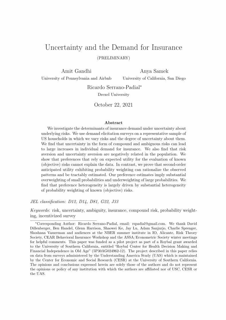
Figure 2 presents the average uncertainty premium at each possible p. Each datapoint shows the size of the range of probabilities associated with it, given by 2ε. Sinceour design includes two range sizes for most of the probabilities, the graph displays twolines, respectively associated with small and big ranges.5

On average, agents exhibit significantly large uncertainty premia at p < 50% whenrange sizes are big, leading to an increase in WTP as high as 100% of the expected loss.Smaller range sizes still elicit a strong response for p < 50%. Uncertainty premiumdecreases with risk probability p, which is consistent with the finding by Abdellaouiet al. (2015) that aversion to compound and ambiguous lotteries increases as winningprobability goes up. Uncertainty premium is less heterogeneous than risk premia, witha standard deviation between 14% and 20%. We do not find major differences inthe uncertainty premium by ability to reduce compound lotteries (see Table B.5 inAppendix B).

Since the typical probability of filing an insurance claim in most insurance marketsis substantially lower than 50%, the fact that we observe large uncertainty premia atp < 50% points to a strong effect of uncertainty on insurance demand.

4.3 Relationship Between Risk and Uncertainty premium

We next look at the correlation between the risk premium and the uncertainty premium,normalized by range size. We do so for each probability p separately to control for thenegative relationship between p and both µ(p) and µ(I).

5Table B.2 in Appendix B shows the average uncertainty premium at each p by group.

8

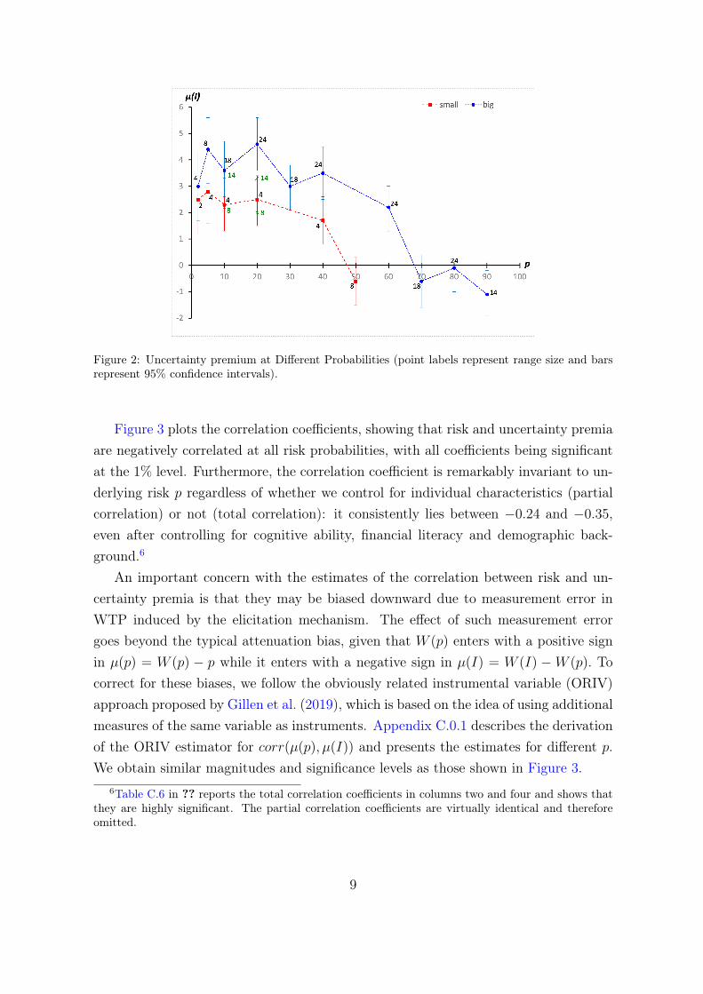
Figure 2: Uncertainty premium at Different Probabilities (point labels represent range size and barsrepresent 95% confidence intervals).

Figure 3 plots the correlation coefficients, showing that risk and uncertainty premiaare negatively correlated at all risk probabilities, with all coefficients being significantat the 1% level. Furthermore, the correlation coefficient is remarkably invariant to un-derlying risk p regardless of whether we control for individual characteristics (partialcorrelation) or not (total correlation): it consistently lies between −0.24 and −0.35,even after controlling for cognitive ability, financial literacy and demographic back-ground.6

An important concern with the estimates of the correlation between risk and un-certainty premia is that they may be biased downward due to measurement error inWTP induced by the elicitation mechanism. The effect of such measurement errorgoes beyond the typical attenuation bias, given that W (p) enters with a positive signin µ(p) = W (p) − p while it enters with a negative sign in µ(I) = W (I) −W (p). Tocorrect for these biases, we follow the obviously related instrumental variable (ORIV)approach proposed by Gillen et al. (2019), which is based on the idea of using additionalmeasures of the same variable as instruments. Appendix C.0.1 describes the derivationof the ORIV estimator for corr(µ(p), µ(I)) and presents the estimates for different p.We obtain similar magnitudes and significance levels as those shown in Figure 3.

6Table C.6 in ?? reports the total correlation coefficients in columns two and four and shows thatthey are highly significant. The partial correlation coefficients are virtually identical and thereforeomitted.

9

Figure 3: Correlation Coefficients between Risk Premium and Uncertainty Premium.

4.4 External Validity

Our empirical results are confirmed by a companion laboratory experiment with about120 undergraduate students at the University of Wisconsin-Madison and by the analysisof publicly available experimental data. The experiment design included a similar set ofdecision questions. We also added an additional treatment for all subjects, multiplica-tive risks to check the robustness of our results to alternative forms of compound risks.Elicitation mechanisms and payments were similar to those in the survey. Appendix Hprovides a full description of the experiment as well as detailed results.

We find that both risk and uncertainty premia are decreasing in risk probabilityp (Figure H.5). The only major difference is that subjects in the experiment weresignificantly less risk averse. In addition, risk and uncertainty premia exhibit a neg-ative correlation of similar magnitude: estimates lie between −0.24 and −0.35, evenafter controlling for both measurement error and personal characteristics (Table H.10).Finally, we analyze covariates of uncertainty premium with the experimental data andfind that qualitatively similar results (see Appendix H.4).

Our analysis of the correlation between risk and uncertainty premium using datafrom three prominent experimental studies on uncertainty preferences (Halevy, 2007;Abdellaoui et al., 2015; Chew et al., 2017) shows that correlation coefficients are sig-nificantly negative and large in magnitude (see Appendix C.0.2). In a recent paper,Chapman et al. (2020) find a mild negative correlation using objective lotteries andbets on ambiguous urns.

10

5 Uncertainty Preferences

We focus on two main families of preferences, namely, EU-based preferences, i.e., thosethat reduce to expected utility (EU) when evaluating known risks, and probability-weighting preferences which apply non-identity weights to probabilities.

The family of EU-based preferences includes most of the proposed models of uncer-tainty preferences: α-maximin expected utility and variational preferences (Maccheroniet al., 2006), which include maximin expected utility (Gilboa and Schmeidler, 1989)and multiplier preferences (Hansen and Sargent, 2001) as special cases, as well assmooth ambiguity preferences (Klibanoff et al., 2005) and uncertainty averse prefer-ences Cerreia-Vioglio et al. (2011). Since preferences reduce to EU under known risks.That is, the value of binary risk (p,−1; 1− p, 0) involving a loss of −1 with probabilityp for an agent with initial wealth w is given by

EU(p) = pu(w − 1) + (1− p)u(w). (1)

As show below, EU-based preferences cannot explain the data on WTP for insur-ance against known risks, unless we resort to non-standard functional forms of utility.In contrast, uncertainty preferences involving probability-weighting can generate riskpremium patterns similar to those illustrated in Figure 1. Two leading examples arerecursive anticipated utility (Segal, 1987) and multiple priors–multiple weighting pref-erences (Dean and Ortoleva, 2017). We restrict attention to the former since it allowsfor flexible weighting functions, whereas the latter requires concave probability weight-ing functions, which we show below cannot explain the risk premium data.

The idea behind recursive anticipated utility is to represent unknown risks as atwo-stage lottery and to apply probability weights recursively. The second-stage lot-tery represents know risks, in our case (p,−1; 1 − p, 0), while the first stage lottery isa probability distribution over p, e.g., U [p− ε, p + ε], representing the decision maker(DM) beliefs about p. Recursive anticipated utility evaluates unknown risks by firstobtaining certainty equivalents of second-stage lotteries, and then evaluate the distri-bution over certainty equivalents induced by the first-stage lottery. In order to applythese preferences to ambiguous risks, it is assumed that the DM has a subjective prob-ability distribution F (p) over known risks.

While recursive anticipated utility uses the same weighting function for both stages,we allow for different probability weighting functions across stages. We call such prefer-ences second order anticipated utility (SOAU)and they are characterized by probability-weighting functions πk and utility functions ui at each stage k = 1, 2. Both πk and uk

11

are increasing with πk(0) = 0 and πk(1) = 1.

Known risks (p,−1; 1−p, 0) are evaluated by applying weighting function π2 to lossprobability p and by using u2 to evaluate changes to final wealth.7 Accordingly, theDM’s valuation of p is given by

V (p) = π2(p)u2(w − 1) + (1− π2(p))u2(w). (2)

To isolate the effect of probability weighting, consider the case of linear utility u2(x) =

x. The certainty equivalent of risk p is −π2(p) and thus the risk premium is given byµ(p) = π2(p)− p.

The evaluation of unknown risk I given by probability distribution F (p) over knownrisks involves the evaluation of certainty equivalents using utility u1 and the applicationof weighting function π1 to the distribution of certainty equivalents induced by F.

Let y(p) be the certainty equivalent of risk p, and G(y) the distribution of certaintyequivalents. If G is continuous and has full support in [y, y], the value of I is given by

V (I) = u1(y) +

y∫y

u′1(y)(1− π1(G(y))dy. (3)

The next proposition characterizes the value of unknown risks of the form I(p, ε) =

U [p−ε, p+ε] with ε ∈ (0,min{p, 1−p}] under SOAU with linear utility u1(x) = u2(x) =

x. Assuming linear utility isolates the role of probability weighting in explaining thedata. All proofs are in Appendix D.

Proposition 1. The value of unknown risk I(p, ε) under SOAU with linear utility isgiven by

Vw(I(p, ε)) = −π2(p− ε)− 2ε

1∫0

π′2(p+ ε(2z − 1))π1 (1− z) dz. (4)

In addition, the uncertainty premium of I(p, ε) is

µ(I(p, ε)) = ε

1∫0

[π′2(p+ εz)π1

(1− z

2

)− π′2(p− εz)

(1− π1

(1 + z

2

))]dz. (5)

7The weighting function is applied over the cdf of outcomes. Alternative formulations involveapplying weights πk(z) = 1−πk(1− z) to the decumulative distribution of outcomes. Following Segal(1987), we use this formulation since it is more convenient when dealing with binary risks.

12

Since the functional form of the uncertainty premium does not lend itself to an easyinterpretation, we define the “marginal uncertainty premium” µ0(p) as the limit of theuncertainty premium, normalized by range size, as ε → 0. The uncertainty premiumassociated with unknown risk I(p, ε) can be well approximated by εµ0(p) as long as π2

exhibits little curvature in the range [p− ε, p+ ε].

Proposition 2. Let µ0(p) := limε→0µ(I(p,ε))

εdenote the marginal uncertainty premium

at p. SOAU with linear utility implies that

µ0(p) = π′2(p)(2Eπ1 − 1), (6)

where Ew1 =∫ 1

0π1(z)dz is the expected value of first-stage probability weights.

Expression (6) shows that the marginal uncertainty premium only depends on thesensitivity of the risk premium to changes in p, measured by the slope of π2, and on theaverage of first stage weights (Eπ1). In particular, µ0(p) is increasing in the averagefirst-stage weight π1, being positive whenever there is overweighting on average, i.e.,Ew1 > 0.5. In addition, the more sensitive the risk premium is to changes in p the largerthe magnitude of µ0(p). Intuitively, individuals whose risk attitudes are insensitive tochanges in loss probability exhibit little variation in WTP for insurance across differentp, and thus do not react strongly to the (initial) introduction of uncertainty.

Next, we provide a series of results showing that, while EU-based preferences cannotexplain the pattern exhibited by risk premium, SOAU preferences can rationalize thethree key empirical facts documented above.

5.1 Risk Premium

As the next proposition formally establishes, EU-based models cannot explain theswitch from risk aversion to risk loving as p goes up without resorting to non-standardutility functions involving concave-then-convex utility at small stakes. We also showin Appendix E that adding a reference point (deterministic or stochastic) to the utilityfunction does not help reconcile the model with the data. In contrast, a probabilityweighting function featuring overweighting of small probabilities and underweighting oflarge ones can rationalize the behavior of the risk premium. An example is the inverteds-shaped weighting function commonly found in experiments on risk prefrences (e.g.,Gonzalez and Wu, 1999).

Proposition 3. Assume that there exists p∗ ∈ [0, 1] such that µ(p) > 0 for p < p∗ andµ(p) < 0 for p > p∗.

13

(i) Expected utility: if the DM has initial wealth w and maximizes expected util-ity under known risks then the upper convex envelope of u(x) is below the lineconnecting u(w − 1) and u(w) for all x ∈ (w − 1, w − p∗) and its lower concaveenvelope is above such line for all x ∈ (w − p∗, w).

(ii) Probability-weighting: if the DM maximizes anticipated utility with linear util-ity then π2(p) > p for p ∈ [0, p∗) and π2(p) < p for p ∈ (p∗, 1].

5.2 Uncertainty premium

SOAU preferences can rationalize the pattern illustrated in Figure 2. To see how, recallthat the marginal uncertainty premium at small ranges is given by π′2(p)(2Eπ1 − 1).

Hence, if preferences exhibit overweighting of 1st-stage probabilities on average (Eπ1 >

0.5) and a 2nd-stage weighting function π2(p) that is steeper at smaller p, then themarginal uncertainty premium is larger at smaller p.

5.3 Correlation between Risk and Uncertainty Premia

The next result provides two possible ways by which a population of individuals withSOAU preferences can exhibit a negative correlation between risk and uncertaintypremia. The first one involves more risk averse individuals being less sensitive tochanges in risk than comparatively less risk averse individuals. This seems like a naturalbehavioral explanation: more risk averse individuals have a stronger incentive to avoidrisks and thus might be less sensitive to variation in underlying risks. Intuitively, theymay be cautious and willing to ‘overpay’ for insurance, regardless of whether underlyingrisks turn out to be smaller or larger than expected. The second explanation is lessplausible since it involves a negative relationship between probability weighting acrossstages, i.e., individuals who have higher second order weights exhibit lower first-orderweights. Such negative relation is hard to reconcile with the notion that risk averseagents dislike ‘randomness.’

Proposition 4. Consider two DM i, j satisfying π2i(p) > π2j(p) for some p ∈ (0, 1).

Then µi(p) > µj(p) and

(i) if π′2i(p) < π′2j(p) and Eπ1i ≤ Eπ1j then µ0i(I(p, ε)) < µ0j(I(p, ε));

(ii) if π′2i(p) ≤ π′2j(p) and Eπ1i < Eπ1j then µ0i(I(p, ε)) < µ0j(I(p, ε)).

The proof is immediate and therefore omitted.

14

One way to test whether SOAU can generate the negative correlation is to estimatethe slope of π2 and the average of first-stage weights Eπ1 at the individual level usingthe following two-step approach. First, for each subject i we estimate π′i2 by running thefollowing linear regression using the observations t = 1, · · · , 5 on WTP for insuranceagainst known risks:

Wit = ai + bipit + νit, t = 1, · · · , 5. (7)

Since W (p) = π2(p), bi is an estimate of π′i2(p). Second, we regress bi on the uncer-tainty premium associated with unknown risks, normalized by range size:

µitεit

= αkbit + ξit. (8)

Since µ0 = π′2(p)(2Eπ1 − 1) we can estimate Eπ1 using Eπi1 = αk+12. Table 2 presents

the average estimates of π′i2(p) and Eπ1 in the population, as well as its cross-sectionalcorrelation with risk and uncertainty premia. The latter confirms the hypothesis thatrisk averse agents exhibit lower sensitivity to changes in underlying risk probabilities,inducing a negative correlation between risk and uncertainty premia. Figure 4 showsthat such negative correlation is mostly driven by individuals with the lowest sensitivity.Specifically, individuals with π′i2 estimates at the bottom quintile of its distributionexhibit significantly higher risk premium and significantly lower uncertainty premiumthan the rest of subjects.

Table 2: Components of uncertainty premium

Regression Estimates

Estimate Average Std. error

π′2(p) 0.61 0.59Eπ1 0.52 1.06

Correlationa

Risk premium Info premiumπ′2(p) -0.15∗∗∗ 0.12∗∗∗Eπ1 -0.01 0.02∗∗∗

No. Obs. 4,442a Statistical significance: *p-value < 0.10, **p-value < 0.05, ***p-value < 0.01.

15

Figure 4: Average Risk and uncertainty premium at different estimates of π′i2.

6 Preference Estimation

This section presents our approach to estimate the distribution of SOAU preferencesin the population and analyzes some of its key features, namely, the typical shape ofweighting functions, the degree of heterogeneity and the distribution of preferencesacross different socio-demographic characteristics.

Our approach is based on the decomposition of WTP into the sum of risk anduncertainty premium, which under linear utility takes on the following form by Propo-sition 1:

W (I(p, ε)) = p+ µ(p) + µ(I(p, ε))

= π2(p) + ε

1∫0

[π′2(p+ εz)π1

(1− z

2

)− π′2(p− εz)

(1− π1

(1 + z

2

))]dz. (9)

We impose a parametric form on πk and estimate them at the individual level usinga hierarchical Bayesian model. Specifically, we assume that weighting functions in (9)have a 2-parameter Prelec functional form:

πk(p) = e−βk(− log(p))αk , αk, βk > 0, k = 1, 2. (10)

This functional form is commonly used to model rank-dependent utility and allows forlinear, concave, convex, as well as s-shaped and inverted s-shaped weighting functions,as illustrated by Table 3 and Figure 5. Lower values of βk globally lead to higherweights πk(p), i.e., to comparatively higher risk aversion, while parameter αk mostlyaffects the shape of πk, determining whether small probabilities are overweighted and

16

large probabilities underweighted (α < 1) or vice versa (α > 1).8 The Prelec weighting

Table 3: Prelec weighting function

Shape of πk αk βkLinear 1 1Concave 1 < 1Convex 1 > 1

Inverted s-shape < 1 anys-shape > 1 any

function crosses the diagonal once at p∗ = e−β1/(1−α) for all α 6= 1. Accordingly, α < 1

implies overweighting of probabilities in [0, p∗]. Note that e−β1/(1−α) is decreasing in βfor all α < 1, implying that smaller β lead to a larger interval [0, p∗] of overweightedprobabilities. Let θ = (α1, β1, α2, β2) be the parameter vector of Prelec weighting

αk = 1 βk = 1

Figure 5: Prelec weighting functions for different values of βk (left) and αk (right).

functions (10) and let W (·; θ) denote the resulting WTP function given by (9). Ourgoal is to estimate the distribution of θ in the population. To do so, we assume thatagent i’s observed WTP for insurance against Iit = I(pit, εit) is given by the randomvariable Wit whose mean is determined by W (Iit; θi), where θi represents the agent’sweighting function parameters. Letting Wit to be random allows for the possibility of

8Specifically, the slope of πk(p) at p = 0 is infinity for αk < 1 and zero for αk > 1, whereas theopposite is true at p = 1.

17

mistakes or for random preferences. Notice that, sinceW (Iit; θi) falls inside the interval(0, 1) for p ∈ (0, 1), we could assume that Wit follows a continuous distribution withsupport in (0, 1) such as the beta distribution. However, a non-negligible subset ofsubjects sometimes report WTP of zero or one. Accordingly, we instead assume thatWit follows a flexible zero-one inflated beta distribution, which allows for the possibilitythat Wit takes on values in {0, 1}. The distribution has two point masses, at 0 and 1,and follows a beta distribution on (0, 1). That is, Wit follows mixture distribution

f(w|Iit, θi, q, q1, φ) =

q(1− q1) w = 0

qq1 w = 1

(1− q)Beta(W (Iit; θi)φ, (1−W (Iit; θi))φ) w ∈ (0, 1),

(11)

where q = Pr(Wit ∈ {0, 1}), q1 = Pr(Wit = 1|Wit ∈ {0, 1}), and φ is the precisionof the beta distribution. Unlike the weighting function parameter vector θi, which isallowed to vary across individuals, we set these three parameters at the populationlevel since we only have ten observations per individual.

We next build a hierarchical model by assuming that αik and βik are drawn frompopulation-level distributions with support on the positive real line. Specifically, weset the prior distribution of αik for k = 1, 2 to be lognormal, with the population-levelmean and standard deviation of logαik given by α and σα, respectively. Similarly, theprior distribution of βik is lognormal with parameters β and σβ.

We close the model by specifying hyperprior distributions for population-level pa-rameters. First, we assume a standard normal prior for α and β, which is centeredaround the values associated with linear probability weighting and its unit varianceyields an informative but dispersed prior.9 Second, we choose a half t-student prior forstandard deviations of Prelec parameters θi. Third, we choose a gamma prior for theprecision of the Beta distribution φ. Finally, we let the probability parameters q0 andq1 to have beta priors given by Beta(1, 1).10

9For values of α or β larger than five the weighting function becomes very close to a step function,so having a vague hyperprior that places a substantial mass above those values is not going to lead tosignificantly different weighting functions while affecting the ability of the model to converge.

10We have tried alternative hyperprior specifications and have not found significant differences inour estimates.

18

Accordingly, our hierarchical model is given by

Wit ∼ f(·|Iit, θi, q0, q1, φ), θi = (α1i, β1i, α2i, β2i)

αik ∼ Lognormal(α, σα), k = 1, 2

βik ∼ Lognormal(β, σβ), k = 1, 2

α ∼ Normal(0, 1)

β ∼ Normal(0, 1) (12)

σα ∼ Half-student t(3, 0, 2.5)

σβ ∼ Half-student t(3, 0, 2.5)

φ ∼ Gamma(1, 2)

qh ∼ Beta(1, 1), h = 0, 1.

Our main goal is to estimate the posterior distribution of θi for each subject in thesample, and use the estimated posteriors to learn about the distribution of uncertaintypreferences in the population, e.g., the distribution of the individual median valuesof θi. In order to do so, we excluded 245 individuals (5.4% of the sample) reportingWTP of always zero or always one in all their choices. Such choices either reflect non-truthfull responses or are associated with infinite degrees of risk love and risk aversion,respectively.

The estimation involves two main hurdles. First, the model is a high-dimensionalnon-linear model. Second, computing the distribution of WTP involves an integralwith no closed-form solution. These features make the model difficult to estimate andcomputationally demanding. To overcome these hurdles we code and fit our model inStan (Stan Development Team, 2019), a probabilistic modeling language that allowsfor Bayesian inference with Markov Chain Monte Carlo (MCMC) sampling. Stan isideally suited for non-linear models and provides built-in functions such as numericalintegration. In addition, it has an adaptive sampling algorithm (No U-turn sampleror NUTS) that facilitates MCMC convergence and allows for within-chain parallelcomputing to speed up the estimation.11 The estimation involved two chains withdifferent starting values and 2,000 iterations each. Standard convergence tests weresatisfactory, with almost all parameters exhibiting effective sample sizes greater than0.75 (see Appendix F for details).

Figure 6 depicts the posterior distributions of individual median values for the fourPrelec parameters and the distribution of individual-level standard deviations, while

11We fit our model using the R interface CmdStanR (Gabry and Češnovar, 2021).

19

Table 4 presents the population-level estimates.12 The distributions of medians give ameasure of heterogeneity of weighting functions in the population while the std. devia-tion distributions reflect the precision of individual-level estimates. Summary statisticsof these distributions are presented in Table 4. The distribution of median values re-

Median Std. Deviation

Figure 6: Posterior density of median values (left) and standard deviations (right) of θi. Red linesrepresent distribution medians.

veals several aspects of risk and uncertainty preferences. First, α2i and β2i exhibitsubstantial dispersion, implying that the 2nd-stage weighting function π2i. In contrast,median values of α1i and β1i are much more concentrated leading to a relatively ho-mogeneous 1st-stage weighting function π1i. Second, individual estimates of 2nd-stageweighting parameters are much more precise than 1st-stage estimates given that theformer exhibit much lower standard deviations. This is likely due to the fact that, since1st-stage weights only affect the uncertainty premium while 2nd-stage weights affectboth the risk and uncertainty premia, all individual observations are effectively used toestimate α2i, β2i while one half of the observations contain information about α1i, β1i.

The population-level parameter estimates in Table 4 help us measure the tendencyto report extreme values of WTP as well as the degree of randomness/deviations ofWTP responses with respect to SOAU preferences. On average, the estimated proba-

12We obtain similar results using mean rather than median values.

20

Table 4: Model Estimates: Population-level Parameters

Parameter Median Std. deviation

q0 0.0688 0.0012q1 0.852 0.0071φ 16.2 0.140α -0.831 0.0137β -0.222 0.0096σα 0.768 0.0122σβ 0.639 0.0076Log Probabilitya 6560 137

No. Obs. 39,950No. Individuals 4,268a Unnormalized log density of the model.

bility of reporting WTP of 0 or 1 is about 7%, with most of these choices being one(85%). This gives us a rough measure of irrationality, in the sense that such valuesimply a violation of stochastic dominance. The precision of the beta distribution isabout 16, which suggests that, while WTP is clearly informed by preferences it exhibitssubstantial randomness.13

What do these parameter distributions tell us about the distribution of individualpreferences? First, they show that the vast majority of individuals exhibit invertedS-shape weighting functions in both probability stages, given that median values of α1i

are below one, while α2i is lower than one for 93% of individuals. In addition, almostall median values of β1i and a majority of β2i are below one, implying overweighting ofprobabilities in a range [0, p∗] with p∗ > e−1 ≈ 0.368.14

To learn more about the distribution of SOAU preferences we look at the joint den-sity of weighting parameters (αik, βik) for k = 1, 2, shown in the top row of Figure 7.Confirming the above results regarding marginal distributions, the joint distribution of(αi2, βi2) is highly dispersed, with most of the mass roughly placed in the lower triangleof rectangle [0, 1.5] × [0, 3]. This implies that, despite wide heterogeneity of risk pref-erences, virtually no agent exhibits risk love at low probabilities and αi2 and βi2 arenegatively correlated. The peak of the joint density, depicted in the bottom-left graphof Figure 7, occurs at αi2 = 0.86, βi2 = 0.92, leading to a weighting function relatively

13For instance, if the mean WTP is 0.5, the interquartile range associated with a precision of 16.2is [0.416, 0.584].

14Since p∗ = e−β1/(1−α)

is decreasing in β for all α < 1, the smallest p∗ when β ≤ 1 is associatedwith b = 1.

21

close to the risk neutral benchmark. Nonetheless, the joint distribution is quite asym-metric, with αi2 typically falling well below one, i.e., most agents exhibit substantialrisk aversion (overweighting) at low probabilities and risk loving (underweighting) athigh probabilities. This is illustrated by the weighting function associated with themedian (of median) values of αi2 and βi2 (see bottom-left graph of Figure 7).

In contrast, the joint density of (αi1, βi1) is highly concentrated along the diagonalof rectangle [0.4, 0.5] × [0.5, 1], with the mode given by αi1 = 0.44, βi1 = 0.8. Accord-ingly, these estimates suggest that all agents in the population significantly overweigh(underweighs) 1st-stage probabilities below (above) 0.5, as illustrated in bottom-rightgraph of Figure 7).

Figure 7: Top panel: Posterior joint density of median values of (αi2, βi2) (left) and (αi1, βi1) (right);white lines represent median values of each parameter. Bottom panel: 2nd-stage weighting function(left) and 1st-stage weighting function (right); the mode represents the weighting function associatedwith the mean of the distribution and the median refers to the weighting function associated with themedian (of median) values of each parameter.

The dispersion of 2nd-stage weighting functions leads to wide heterogeneity in risk

22

preferences. Since 1st-stage weighting functions are very homogeneous one might con-clude that heterogeneity in risk preferences drives heterogeneity in uncertainty pref-erences. However, this is unclear because the uncertainty premium depends on theslope of π2 and the level of π1. One way to understand the relative contribution ofeach weighting function to the heterogeneity of uncertainty preferences is to lookat their relative contribution to the variation of the marginal uncertainty premiumµ0(p) = π′2(p)(2Eπ1 − 1). Using the above joint distribution we compute the standarddeviation of π′2(p) for p ∈ (0.1, 0.9) and the standard deviation of 2Eπ1.

15 We find thatthe standard deviation of π′2(p) ranges between 0.26 and 0.44, while the std. deviationof 2Eπ1 is about 0.12. These differences are much smaller than the large differencesin heterogeneity between π2 and π1 exhibited by the joint distributions in Figure 7,although 2nd-stage weights still contribute between two to four times more to theheterogeneity of marginal uncertainty premia than 1st-stage weights.

6.1 Sociodemographic Differences

We next analyze potential differences in the distribution of preferences across differentsociodemographic characteristics. Specifically, we plot the joint distribution of 2nd-stage weighting parameters by income, age and gender (Figure 8), and also by financialliteracy and cognitive ability (Figure 9).

There are some differences across groups, with higher income individuals and menexhibiting less probability mass at low values of (αi2, βi2) than lower income individualsand women respectively, but overall heterogeneity remains substantial across groups.The starkest differences appear when we compare groups by financial literacy andcognitive ability test scores. The distribution of (αi2, βi2) is more concentrated athigher values for individuals with scores above the median, with very little mass inthe rectangle [0, 0.5] × [0, 1]. In addition, both have a peak close to linear weighting.In contrast, the distribution of those with scores lower than the median score exhibitsubstantial mass in [0, 0.5]× [0, 1].

We do not find any meaningful differences in the joint distribution of 1st stageweights across these characteristics, and thus we do not present them here. This is notsurprising, given that the distribution (αi1, βi1) is very concentrated.

These results are confirmed by the estimates from regressing risk and uncer-15We avoid extreme values of p since the slope of π2 tends to infinity (or zero) under the Prelec

functional form.

23

Figure 8: Joint distribution of median values of (α2i, β2i) by selected demographics.

24

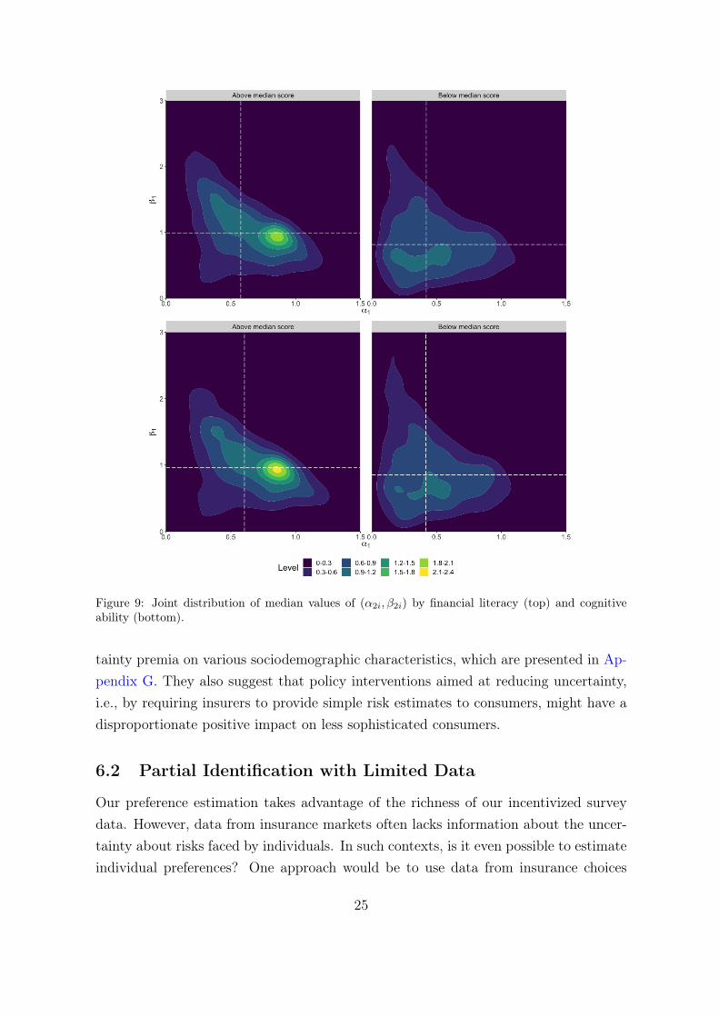
Figure 9: Joint distribution of median values of (α2i, β2i) by financial literacy (top) and cognitiveability (bottom).

tainty premia on various sociodemographic characteristics, which are presented in Ap-pendix G. They also suggest that policy interventions aimed at reducing uncertainty,i.e., by requiring insurers to provide simple risk estimates to consumers, might have adisproportionate positive impact on less sophisticated consumers.

6.2 Partial Identification with Limited Data

Our preference estimation takes advantage of the richness of our incentivized surveydata. However, data from insurance markets often lacks information about the uncer-tainty about risks faced by individuals. In such contexts, is it even possible to estimateindividual preferences? One approach would be to use data from insurance choices

25

across domains, e.g., auto insurance and home insurance, to partially estimate pref-erences by using a linear approximation of the 2nd-stage weighting function π2. Sinceinformation and uncertainty about risks varies across domains, we can use them asproxies for uncertainty, while the linear approximation makes the uncertainty premiumproportional to the slope of π2. Specifically, under linear approximation π2(p) = a+ bp,the WTP for insurance against unknown risk (p, ε) is given by

W (p, ε) = π2(p) + εµ0(p) = a+ bp+ εb(2Eπ1 − 1) = a+ bp+ cε. (13)

In principle, we can estimate this linear regression from data {Wit, pit, εt}i, where trepresents the insurance domain. While pit and εt are not observed, pit can be measuredusing empirical claim rates, as is the typically done in the empirical insurance literature,and the volatility of claim rates in each domain can serve as a proxy for εt.

Expression (13) also serves to illustrate the potential effects of abstracting fromthe presence of uncertainty in the estimation of risk preferences. As an example, notincluding εt in the linear regression implied by (13) translates into omitted variablebias, leading to a biased intercept and a higher (lower) slope estimates depending onwhether risk p and uncertainty ε are positively or negatively correlated.

7 Conclusion

Our study uncovers the impact of uncertainty on insurance demand and uncovers keyfeatures about the nature and distribution of risk and uncertainty attitudes. There areseveral takeaways from our analysis, which point to methodological changes, policy in-terventions and potential avenues for future research. Such implications of our analysisacquire particular relevance given that we find similar patterns across multiple datasources.

Methodologically, our work emphasizes the need to account for uncertainty in theestimation of preferences and suggests ways to do so even with limited data. It alsohighlights the need to develop models of uncertainty preferences that incorporate prob-ability weighting and proposes a class of preferences amenable to empirical estimation.From an econometrics perspective, our preference estimation exercise illustrates the po-tential of Bayesian hierarchical methods to obtain distributional estimates that allowfor a comprehensive analysis of agent heterogeneity.

The paper highlights that different types of information frictions affect markets indifferent ways. Whereas frictions about insurance contracts (e.g., information about

26

coverage, pricing, transaction costs) tend to depress demand for those contracts (Handeland Kolstad, 2015; Bhargava et al., 2017; Handel et al., 2019; Domurat et al., 2019), weshow that uncertainty about risks increases insurance demand and can lead to selectioneffects. These differences imply that friction-mitigation policies aimed at improvingwelfare need to be tailored to the specific frictions being targeted. In particular, policiesaimed at regulating disclosure of known risk estimates can have large welfare effects,primarily benefiting less-sophisticated lower-income consumers. While conducting awelfare analysis is beyond the scope of this paper, we do so in a companion paperGandhi et al. (2020).

Finally, the sources of agents’ reaction to unknown risks remain elusive. Most of thesociodemographic variables traditionally associated with risk attitudes, such as incomeor education, lack explanatory power when it comes to uncertainty preferences. Thisimplies that information frictions cannot be controlled for in empirical work by simplyconditioning on observable characteristics.

27

ReferencesAbdellaoui, Mohammed, Peter Klibanoff, and Lætitia Placido, “Experiments on

Compound Risk in Relation to Simple Risk and to Ambiguity,” Management Science, 2015,61 (6), 1306–1322.

Barseghyan, Levon, Francesca Molinari, Ted O’Donoghue, and Joshua C Teit-elbaum, “The nature of risk preferences: Evidence from insurance choices,” AmericanEconomic Review, 2013, 103 (6), 2499–2529.

, Jeffrey Prince, and Joshua C Teitelbaum, “Are Risk Preferences Stable AcrossContexts? Evidence from Insurance Data,” American Economic Review, 2011, 101 (2),591–631.

Becker, Gordon M, Morris H DeGroot, and Jacob Marschak, “Measuring Utility bya Single-Response Sequential Method,” Behavioral Science, 1964, 9 (3), 226–232.

Bell, David E, “Disappointment in decision making under uncertainty,” Operations research,1985, 33 (1), 1–27.

Bhargava, Saurabh, George Loewenstein, and Justin Sydnor, “Choose to Lose: HealthPlan Choices from a Menu with Dominated Option,” The Quarterly Journal of Economics,2017, 132 (3), 1319–1372.

Cerreia-Vioglio, Simone, Fabio Maccheroni, Massimo Marinacci, and Luigi Mon-trucchio, “Uncertainty averse preferences,” Journal of Economic Theory, 2011, 146 (4),1275–1330.

Chapman, Jonathan, Mark Dean, Pietro Ortoleva, Erik Snowberg, and ColinCamerer, “Econographics,” Technical Report 2020. Working paper.

Chew, Soo Hong, Bin Miao, and Songfa Zhong, “Partial Ambiguity,” Econometrica,2017, 85 (4), 1239–1260.

Cohen, Michele, Jean-Yves Jaffray, and Tanios Said, “Experimental comparison of in-dividual behavior under risk and under uncertainty for gains and for losses,” Organizationalbehavior and human decision processes, 1987, 39 (1), 1–22.

Dean, Mark and Pietro Ortoleva, “Allais, Ellsberg, and preferences for hedging,” Theo-retical Economics, 2017, 12 (1), 377–424.

Dillenberger, David and Uzi Segal, “Skewed Noise,” Journal of Economic Theory, 2017,169 (C), 344–364.

Domurat, Richard, Isaac Menashe, and Wesley Yin, “The Role of Behavioral Frictionsin Health Insurance Marketplace Enrollment and Risk: Evidence from a Field Experiment,”National Bureau of Economic Research, Working Paper No. 26153 2019.

Einav, Liran, Amy Finkelstein, and Jonathan Levin, “Beyond Testing: EmpiricalModels of Insurance Markets,” Annual Review of Economics, 2010, 2, 311.

28

, , Iuliana Pascu, and Mark R Cullen, “How General are Risk Preferences? ChoicesUnder Uncertainty in Different Domains,” American Economic Review, 2012, 102 (6), 2606–2638.

Einhorn, Hillel J and Robin M Hogarth, “Decision making under ambiguity,” Journalof Business, 1986, pp. S225–S250.

Fischbacher, Urs, “z-Tree: Zurich Toolbox for Ready-Made Economic Experiments,” Ex-perimental Economics, 2007, 10 (2), 171–178.

Frederick, Shane, “Cognitive Reflection and Decision Making,” The Journal of EconomicPerspectives, 2005, 19 (4), 25–42.

Gabry, Jonah and Rok Češnovar, cmdstanr: R Interface to ’CmdStan’ 2021. https://mc-stan.org/cmdstanr.

Gandhi, Amit, Anya Samek, and Ricardo Serrano-Padial, “On Information and theDemand for Insurance,” 2020. working paper.

Gilboa, Itzhak and David Schmeidler, “Maxmin expected utility with non-unique prior,”Journal of mathematical economics, 1989, 18 (2), 141–153.

Gillen, Ben, Erik Snowberg, and Leeat Yariv, “Experimenting with Measurement Error:Techniques with Applications to the Caltech Cohort Study,” Journal of Political Economy,2019, 127 (4), 1826–1863.

Gonzalez, Richard and George Wu, “On the shape of the probability weighting function,”Cognitive psychology, 1999, 38 (1), 129–166.

Gul, Faruk, “A theory of disappointment aversion,” Econometrica: Journal of the Econo-metric Society, 1991, pp. 667–686.

Halevy, Yoram, “Ellsberg Revisited: An Experimental Study,” Econometrica, 2007, 75 (2),503–536.

Handel, Benjamin R and Jonathan T Kolstad, “Health Insurance for “Humans”: Infor-mation Frictions, Plan Choice, and Consumer Welfare,” The American Economic Review,2015, 105 (8), 2449–2500.

, , and Johannes Spinnewijn, “Information Frictions and Adverse Selection: PolicyInterventions in Health Insurance Markets,” Review of Economics and Statistics, 2019, 101(2), 326–340.

Hansen, LarsPeter and Thomas J Sargent, “Robust Control and Model Uncertainty,”American Economic Review, 2001, 91 (2), 60–66.

Jaspersen, Johannes G, “Hypothetical Surveys and Experimental Studies of InsuranceDemand: A Review,” Journal of Risk and Insurance, 2016, 83 (1), 217–255.

Klibanoff, Peter, Massimo Marinacci, and Sujoy Mukerji, “A smooth model of decisionmaking under ambiguity,” Econometrica, 2005, 73 (6), 1849–1892.

29

Kőszegi, Botond and Matthew Rabin, “A model of reference-dependent preferences,”The Quarterly Journal of Economics, 2006, 121 (4), 1133–1165.

Loomes, Graham and Robert Sugden, “Disappointment and dynamic consistency inchoice under uncertainty,” The Review of Economic Studies, 1986, 53 (2), 271–282.

Maccheroni, Fabio, Massimo Marinacci, and Aldo Rustichini, “Ambiguity aversion,robustness, and the variational representation of preferences,” Econometrica, 2006, 74 (6),1447–1498.

Mauro, Carmela Di and Anna Maffioletti, “Attitudes to risk and attitudes to uncer-tainty: experimental evidence,” Applied Economics, 2004, 36 (4), 357–372.

Outreville, J François, “Risk Aversion, Risk Behavior, and Demand for Insurance: A Sur-vey,” Journal of Insurance Issues, 2014, pp. 158–186.

Prelec, Drazen, “The probability weighting function,” Econometrica, 1998, pp. 497–527.

Segal, Uzi, “The Ellsberg paradox and risk aversion: An anticipated utility approach,” In-ternational Economic Review, 1987, pp. 175–202.

Sprenger, Charles, “An endowment effect for risk: Experimental tests of stochastic referencepoints,” Journal of Political Economy, 2015, 123 (6), 1456–1499.

Stan Development Team, Stan Modeling Language Users Guide and Reference Manual2019. Version 2.27, https://mc-stan.org.

Sydnor, Justin, “(Over) Insuring Modest Risks,” American Economic Journal: AppliedEconomics, 2010, 2 (4), 177–199.

30

Appendix A Descriptive StatisticsTable A.1 presents the summary statistics of the main sociodemographic variables ofhouseholds in the UAS in Surveys 1 and 2.

Table A.1: Descriptive Statistics - UAS

Variable Mean Std. Dev.Age 48.34 15.52Female 0.57 0.49Married 0.59 0.49Some College 0.39 0.49Bachelor’s Degree or Higher 0.36 0.48HH Income: 25k-50k 0.24 0.43HH Income: 50k-75k 0.20 0.40HH Income: 75k-100k 0.13 0.34HH Income: Above 100k 0.20 0.40Black 0.08 0.27Hispanic/Latino 0.10 0.29Other Race 0.10 0.30Financial Literacy (range: 0-100) 67.52 22.11Cognitive Ability 50.70 8.66No. Individuals 4,442

Appendix B Statistical Analysis of WTPIn this section we present the average WTP under known risk (W (p)) and the uncer-tainty premium. We report both averages for the whole sample, and also distinguishingby whether decisions involved ambiguous ranges. Finally, we use our incentivized quizabout reducing compound risks, to contrast average WTP by subjects’ ability to reducecompound lotteries.

Table B.2 presents whole sample averages and reports both whether WTP are dif-ferent from risk probabilities and whether uncertainty premium is significantly differentfrom zero using one-sided paired t-tests.

Ambiguity Tables B.3 and B.4 show the effect of presenting agents with non-ambiguous versus ambiguous ranges. There is no clear effect of ambiguity on the

31

Table B.2: WTP for Insurance: Pooled Compound and Ambiguous Risk

Group 1 Group 2 Group 3 Group 4p W (p)a µ(I)b,c W (p) µ(I) W (p) µ(I) W (p) µ(I)

2 28.2∗∗∗ 2.5∗∗∗ 28.3∗∗∗ 3.0∗∗∗(2) (4)

5 25.8∗∗∗ 2.8∗∗∗ 28.9∗∗∗ 4.4∗∗∗(4) (8)

10 28.5∗∗∗ 3.6∗∗∗ 31.4∗∗∗ 3.5∗∗∗ 31.4∗∗∗ 2.2∗∗∗ 30.9∗∗∗ 2.3∗∗∗(18) (14) (8) (4)

20 34.1∗∗∗ 3.5∗∗∗ 36.8∗∗∗ 2.5∗∗∗ 36.6∗∗∗ 4.6∗∗∗ 37.1∗∗∗ 2.0∗∗∗(14) (4) (24) (8)

30 42.4∗∗∗ 3.0∗∗∗(18)

40 48.1∗∗∗ 3.5∗∗∗ 49.1∗∗∗ 1.7∗∗∗(24) (4)

50 54.7∗∗∗ -0.6∗(8)

60 60.3 2.2∗∗∗(24)

70 66.5∗∗∗ -0.6(18)

80 69.8∗∗∗ -0.1(4)

90 77.9∗∗∗ -1.1∗∗(14)

a Statistical significance of one-sided paired t-test with null hypothesis W (p) > (<) p:*p-value < 0.10, **p-value < 0.05, ***p-value < 0.01.b Statistical significance of one-sided paired t-test with null hypothesis µ(I) > (<) 0:*p-value < 0.10, **p-value < 0.05, ***p-value < 0.01.c Range sizes in parenthesis.

uncertainty premium. Overall, effects seem to be quantitatively of the same order ofmagnitude.

Ability to reduce compound lotteries. Table B.5 shows the average WTP asso-ciated with the range used in the incentivized question that asked subjects to computethe underlying failure probability. There are no substantial differences in uncertaintypremia between those who answered correctly and those who did not correctly reducethe range, except for the last 2 ranges, in which those who reduced the range properlyactually exhibit a higher WTP.

32

Table B.3: WTP for Insurance: Compound Risk I = U [p− ε, p+ ε]

Group 1 Group 2 Group 3 Group 4p W (p)a µ(I)b,c W (p) µ(I) W (p) µ(I) W (p) µ(I)

2 29.2∗∗∗ 2.3∗∗ 28.5∗∗∗ 2.8∗∗∗(2) (4)

5 25.3∗∗∗ 2.6∗∗∗ 29.2∗∗∗ 3.4∗∗∗(4) (8)

10 27.6∗∗∗ 4.1∗∗∗ 32.0∗∗∗ 2.9∗∗∗ 32.0∗∗∗ 2.1∗∗∗ 30.1∗∗∗ 3.0∗∗∗(18) (14) (8) (4)

20 32.8∗∗∗ 3.6∗∗∗ 37.6∗∗∗ 1.7∗∗∗ 37.2∗∗∗ 4.4∗∗∗ 35.9∗∗∗ 2.7∗∗∗(14) (4) (24) (8)

30 41.5∗∗∗ 4.0∗∗∗(18)

40 48.4∗∗∗ 3.9∗∗∗ 49.9∗∗∗ 1.4∗∗(24) (4)

50 53.0∗∗∗ 0.03(8)

60 60.3 3.1∗∗∗(24)

70 66.8∗∗∗ 0.0(18)

80 67.7∗∗∗ 0.8∗(4)

90 78.2∗∗∗ -0.8∗(14)

a Statistical significance of one-sided paired t-test with null hypothesis W (p) > (<) p:*p-value < 0.10, **p-value < 0.05, ***p-value < 0.01.b Statistical significance of one-sided paired t-test with null hypothesis µ(I) > (<) 0:*p-value < 0.10, **p-value < 0.05, ***p-value < 0.01.c Range sizes in parenthesis.

33

Table B.4: WTP for Insurance: Ambiguous Risk I = [p− ε, p+ ε].

Group 1 Group 2 Group 3 Group 4p W (p)a µ(I)b,c W (p) µ(I) W (p) µ(I) W (p) µ(I)

2 27.2∗∗∗ 2.8∗∗∗ 28.1∗∗∗ 3.3∗∗∗(2) (4)

5 26.2∗∗∗ 2.9∗∗∗ 28.7∗∗∗ 5.4∗∗∗(4) (8)

10 29.4∗∗∗ 3.1∗∗∗ 30.7∗∗∗ 4.1∗∗∗ 30.7∗∗∗ 2.4∗∗∗ 31.7∗∗∗ 1.6∗∗∗(18) (14) (8) (4)

20 35.4∗∗∗ 2.9∗∗∗ 36.1∗∗∗ 3.3∗∗∗ 36.1∗∗∗ 4.7∗∗∗ 38.2∗∗∗ 1.2∗∗(14) (4) (24) (8)

30 43.3∗∗∗ 2.0∗∗∗(18)

40 47.8∗∗∗ 3.1∗∗∗ 48.3∗∗∗ 2.0∗∗∗(24) (4)

50 56.4∗∗∗ -1.2∗∗(8)

60 60.3 1.2∗∗(24)

70 66.3∗∗∗ -1.2∗∗(18)

80 71.9∗∗∗ -1.1∗∗(4)

90 77.5∗∗∗ -1.4∗∗(14)

a Statistical significance of one-sided paired t-test with null hypothesis W (p) > (<) p:*p-value < 0.10, **p-value < 0.05, ***p-value < 0.01.b Statistical significance of one-sided paired t-test with null hypothesis µ(I) > (<) 0:*p-value < 0.10, **p-value < 0.05, ***p-value < 0.01.c Range sizes in parenthesis.

Table B.5: WTP by Ability to Reduce Compound Lotteries

Correct IncorrectDecision p W (p)a µ(I)b n W (p) µ(I) n

Range3-7 5 22.6∗∗∗ 2.7∗∗∗ 658 34.2∗∗∗ 2.7∗∗ 2473-17 10 26.3∗∗∗ 3.3∗∗∗ 484 37.3∗∗∗ 3.3∗∗∗ 4178-32 20 30.6∗∗∗ 5.2∗∗∗ 523 42.4∗∗∗ 3.9∗∗∗ 53921-39 30 38.7∗∗∗ 4.0∗∗∗ 655 48.5∗∗∗ 1.2∗ 406a Statistical significance of one-sided paired t-test with null hypothesis W (p) > (<) p:*p-value < 0.10, **p-value < 0.05, ***p-value < 0.01.b Statistical significance of one-sided paired t-test with null hypothesis µ(I) > (<) 0:*p-value < 0.10, **p-value < 0.05, ***p-value < 0.01.

34

Appendix C Robustness and External ValidityC.0.1 Measurement Error Correction

This section provides estimates of the correlation between risk and uncertainty premiumthat correct for potential biases due to measurement error. To formally show theproblem, let W (I) = W (I) + εI be the elicited WTP under information I, where εI isa random variable representing classical measurement error. Accordingly, the elicitedrisk premium is given by µ(p) = µ(p) + εp and the elicited uncertainty premium isgiven by µ(I) = µ(I) + εI − εp. Assuming that measurement errors are independentlydrawn and that they are independent of W (·), the correlation between µ(I) and µ(p)is given by

corr(µ(I), µ(p)) =cov(µ(I), µ(p))− V ar(εp)√

(V ar(µ(I) + V ar(εI − εp))(V ar(µ(p) + V ar(εp)).

Hence, the numerator is negatively biased while the denominator is biased upwards,making both the direction and the size of the bias indeterminate.

However, if we have duplicate measures of the risk premium, µ(p) and µd(p) =µ(p) + εdp we can use µd(p) as an instrument for µ(p) in a regression of µ(I) on µ(p).Since errors are independent across measures the measurement error in µ(I), given byεI − εp, is independent of the measurement error εdp in µd(p), making the latter a validinstrument. Accordingly, the regression coefficient β delivers a consistent estimate ofcov(µ(I), µ(p))

V ar(µ(p)). If, in addition, we have an additional measure µd(I) of the uncertainty

premium, the correlation between the risk and uncertainty premia can be consistentlyestimated using

corr(µ(p), µ(I)) = β

√cov(µ(p), µd(p))

cov(µ(I), µd(I)), (14)

where corr and cov represent sample correlation and covariance, respectively.Gillen et al. (2019) exploit the use of duplicate measures or replicas to obtain not

only consistent but also efficient estimates via stacked IV regressions, one per availablereplica, with the remaining replicas acting as instruments. They call their approachan obviously related instrumental variable (ORIV) regression and show how to obtainconsistent correlation estimates and bootstrapped standard errors.

To obtain replicas of risk and uncertainty premia, we take advantage of the factthat our experimental design elicits subjects’ WTP for insurance for multiple riskprobabilities. Specifically, we use the linear interpolation of risk premium associatedwith the probability points adjacent to p as the second measure of µ(p). That is, ifp′ < p and p′′ > p are the loss probabilities closest to p in the experimental design, thereplicas of risk and uncertainty premia are given by

µd(p) = µ(p′)p′′ − pp′′ − p′

+ µ(p′′)p− p′

p′′ − p′,

35

µd(I) = µ(I ′)p′′ − pp′′ − p′

+ µ(I ′′)p− p′

p′′ − p′,

where I ′ and I ′′ represent the unknown risks respectively associated with p′ and p′′.We normalize uncertainty premium by dividing it by range size and perform the linearinterpolation using the normalized premia.

Table C.6 shows the ORIV correlation for probabilities with adjacent probabilitieson both sides (column three). The estimates are of similar magnitude if not slightlymore negative. These results indicate that the negative relationship between risk anduncertainty premia is not an artifact of measurement error.

Table C.6: Correlation between risk and insurance premia

p correlationa ORIV correlationb

2 -0.312∗∗∗ -5 -0.291∗∗∗ -10 -0.276∗∗∗ -0.310∗∗∗20 -0.241∗∗∗ -0.319∗∗∗30 -0.329∗∗∗ -0.324∗∗∗40 -0.256∗∗∗ -0.353∗∗∗50 -0.347∗∗∗ -0.306∗∗∗60 -0.284∗∗∗ -70 -0.309∗∗∗ -80 -0.267∗∗∗ -90 -0.276∗∗∗ -a Statistical significance: *p-value < 0.10, **p-value < 0.05, ***p-value < 0.01.b p-values for ORIV correlation are computed using bootstrapped standard errors.

C.0.2 Correlation in Existing Experimental Data

The remarkable invariance of our correlation estimates raises the question whetherwe have uncovered a robust feature of uncertainty preferences or whether they arejust a byproduct of our specific survey design. We address this question by replicatingour analysis in our companion laboratory experiment, which is described below, and bycomputing the correlation between risk premium and compound risk premia in the dataof some of the most prominent studies looking at the relationship between ambiguityand compound risk attitudes, namely the papers by Halevy (2007), Abdellaoui et al.(2015) and Chew et al. (2017).

As Table C.6 shows, correlation coefficients are significantly negative in all thedatasets. Interestingly, since the data in Abdellaoui et al. (2015) includes three differentprobabilities we were able to calculate the ORIV correlation for p = 1/2, which turnsout to be identical to the ORIV correlation of −0.3 in our data.16

16Abdellaoui et al. (2015) use compound lotteries in their ‘hypergeometric CR’ treatment, preventing

36

Table C.7: Correlation between risk and insurance premia

p Study N correlation ORIV correlation50 This paper - UAS 1,043 -0.347∗∗∗ -0.306∗∗∗50 This paper - Experiment 119 -0.401∗∗∗ -0.299∗∗∗50 Halevy (2007) - $2 treatment 104 -0.557∗∗∗ -50 Halevy (2007) - $20 treatment 38 -0.542∗∗∗ -8.33 Abdellaoui et al. (2015)c 115 -0.418∗∗∗ -50 Abdellaoui et al. (2015)d 115 -0.365∗∗∗ -0.310∗∗91.67 Abdellaoui et al. (2015) 115 -0.518∗∗∗ -50 Chew et al. (2017) 188 -0.493∗∗∗ -a Statistical significance: *p-value < 0.10, **p-value < 0.05, ***p-value < 0.01.b p-values for ORIV correlation are computed using bootstrapped standard errors.c Correlation between the known risk premium and hypergeometric CR premium.d ORIV correlation from the Abdellaoui et al. (2015) dataset is computed using the average risk premium undersimple lotteries with winning probabilities 1/12 and 11/12 as a replica for the risk premium at probability 1/2.

Appendix D Omitted ProofsProof of Proposition 1. Under linear utility u(x) = x the certainty equivalent of knownrisk (q,−1; 1− q, 0) is −π2(q). Since this expression is decreasing in q, the distributionof certainty equivalents induced by the uniform distribution on [p− ε, p+ ε] is given by

G(y) = Pr(q ≥ π−12 (−y)) = 1− π−1

2 (−y)− p+ ε

2ε=p+ ε− π−1

2 (−y)

2ε,

where π−12 denotes the inverse of π2. In addition, the lowest and highest certainty

equivalents are respectively associated with the highest and lowest loss probabilities,i.e., y = −π2(p+ ε) and y = −π2(p− ε). Accordingly, expression (3) leads to

Vw(I(p, ε)) = −π2(p− ε)−−π2(p−ε)∫−π2(p+ε)

π1

(p+ ε− π−1

2 (−y)

2ε

)dy.

Applying the change of variable t = π−12 (−y) we obtain

Vw(I(p, ε)) = −π2(p− ε)−p+ε∫p−ε

π′2(t)π1

(p+ ε− t

2ε

)dt.

A second change of variable z = t−p+ε2ε

implies that 2εdz = dt and that the new limitsof integration are z = 0 and z = 1, leading to expression (4).

To prove the second part of the proposition, note that the uncertainty premium

us from obtaining a replica of the uncertainty premium given that such lotteries are hard to compareacross p. Nonetheless, the ORIV correction can still be performed by using a replica of the riskpremium at 1/2, obtained via linear interpolation with probabilities 1/12 and 11/12.

37

satisfies Vw(I(p, ε)) = −µ(I(p, ε))− µ(p)− p. Since µ(p) = π2(p)− p, we have that

µ(I(p, ε)) = −π2(p) + π2(p− ε) + 2ε

1∫0

π′2(p+ ε(2z − 1))π1 (1− z) dz.

By the fundamental theorem of calculus we can express π2(p) as

π2(p) = π2(p− ε) +

0∫−ε

π′2(p+ t)dt = π2(p− ε) + 2ε

1/2∫0

π′2(p+ ε(2z − 1))dz,

where the last equality follows from the change of variable z = t+ε2ε. Hence,

µ(I(p, ε)) = −2ε

1/2∫0

π′2(p+ ε(2z − 1))dz + 2ε

1∫0

π′2(p+ ε(2z − 1))π1 (1− z) dz

= −2ε

1/2∫0

π′2(p+ ε(2z − 1)) (1− π1 (1− z)) dz + 2ε

1∫1/2

π′2(p+ ε(2z − 1))π1 (1− z) dz.

The last expression leads to (5) by applying the change of variable z′ = 1− 2z to thefirst integral and z′ = 2z − 1 to the second integral.

Proof of Proposition 2. Dividing both sides of (5) and taking the limit as ε → 0 weobtain

limε→0

µ(I(p, ε))

ε= π′2(p)

1∫0

π1

(1− z

2

)dz +

1∫0

π1

(1 + z

2

)dz − 1

= π′2(p)

2

1/2∫0

π1 (z′) dz′ + 2

1∫1/2

π1 (z′) dz′ − 1

= π′2(p)

2

1∫0

π1 (z′) dz′ − 1

.

Proof of Proposition 3. Part (i): We prove first the condition regarding the lowerconcave envelope. The expected utility of risk (p,−1; 1 − p, 0) is given by pu(w −1) + (1 − p)u(w). A positive risk premium for p ∈ (0, p∗) involves u(w − p) >pu(w − 1) + (1 − p)u(w). Letting x = w − p we get that u(x) > x(u(w) − u(w −1)) + u(w)(1 − w) + wu(w − 1). Since the RHS is linear in x the strict inequalityimplies that we can always find a concave function g(x) satisfying u(x) ≥ g(x) >

38

x(u(w)− u(w − 1)) + u(w)(1− w) + wu(w − 1) for all x ∈ (w − p∗, w). The proof forthe upper convex envelope is similar and therefore omitted.

Part (ii): The risk premium under linear utility u(x) = x is given by µ(p) = π2(p)−pso the condition is immediate.

Appendix E Reference-Dependent PreferencesWe show in this section that adding reference dependence to EU-based uncertaintypreferences cannot explain the risk premium patterns without resorting to non-standardfunctional forms of the utility function.

Reference-dependent preferences involve taking expectations over the utility ofchanges w.r.t. a reference point x∗, given by the function v(x − x∗). Reference pointscan be deterministic or stochastic. Regarding stochastic reference points, which wereintroduced by Kőszegi and Rabin (2006), when evaluating WTP for full insurance, it isnatural to make the lottery (p,−1; 1− p, 0) the reference point. In this case, Sprenger(2015) has shown that stochastic reference point leads to risk neutrality when choosinga deterministic outcome (full insurance), thereby predicting a risk premium equal tozero for all p. Accordingly, we focus on deterministic reference points.

The value of known risk (p,−1; 1−p, 0) for a DM with initial wealth w and referencepoint x∗ is given by

Vr(p) = pv(w − 1− x∗) + (1− p)v(w − x∗). (15)

Two popular choices of reference points are either initial wealth (x∗ = w) or expectedfinal wealth (x∗ = w−p) as in the model of dissapointment aversion (Bell, 1985; Loomesand Sugden, 1986; Gul, 1991). They respectively lead to

Vr(p) = pv(−1) + (1− p)v(0) (16)

andVr(p) = pv(−1 + p) + (1− p)v(p). (17)

The next results shows that for reference-dependent preferences to explain the riskpremium data we would need to resort to non-standard utility functions that switchbetween concavity/convexity or between loss averse/gain loving as wealth changes goabove some threshold p∗ ∈ (0, 1).

Proposition 5. Assume that there exists p∗ ∈ [0, 1] such that µ(p) > 0 for p < p∗ andµ(p) < 0 for p > p∗. If the DM maximizes expected utility v(x− x∗) over gains/losseswith respect to reference point x∗ then

(iii.a) if x∗ = w then the upper convex envelope of v(z) is below the line connectingv(−1) and v(0) for all z ∈ (−1,−p∗) and then its lower concave envelope abovethe line for all z ∈ (−p∗, 0);

(iii.b) if x∗ = w − p then v(0)−v(p−1)1−p > v(p)−v(0)

p(loss averse) for all p ∈ [0, p∗) and

v(0)−v(p−1)1−p < v(p)−v(0)

p(gain loving) for all p ∈ (p∗, 1].

39

Proof. Part (iii.a): If the reference point is current wealth, then the expected valueof risk (p,−1; 1 − p, 0) is given by pv(−1) + (1 − p)v(0). A positive risk premiumimplies v(−p) > pv(−1)+(1−p)v(0). Hence, the proof follows from applying the sameargument in the proof of part (i) of Proposition 3 to v instead of u for the range oflosses (−p∗, 0).

Part (iii.b): If the reference point is expected final wealth y− p, then the expectedvalue of risk (p,−1; 1−p, 0) is given by pv(p−1)+(1−p)v(p). A positive risk premiumimplies

v(0) > pv(p− 1) + (1− p)v(p)⇒ p (v(0)− pv(p− 1)) > (1− p) (v(p)− v(0)) ,

which proves the condition.

Appendix F Bayesian EstimationThis section presents some convergence tests of the MCMC sampling both within andbetween chains. Initial values for chain 1 were set to α = −0.7, β = −0.36, σα = σβ =0.4, φ = 4, q = 0.1, q1 = 0.8 and αi = β = i = 0.5 for all i. Initial values for chain 2were set to α = β = 0.1, σα = σβ = 2, φ = 2, q = 0.3, q1 = 0.6 and αi = β = i = 1.1 forall i.

Figure F.1 shows that the traces of the last (post warm-up) 1,000 iterations of bothchains mix well, with the two chains exploring the same region of parameter values.Overall, there was only one divergent iteration out of 2,000.

Figure F.1: Traces of selected parameters.

A typical statistic to check for convergence to a common distribution is the split-R, which measures the ratio of the average variance of draws within each chain to

40

the variance of the pooled draws across chains. Such ratios should be one if the chainshave converged. If the chains have not converged to a common distribution, the split-Rstatistic will be greater than one. A common threshold for divergence is 1.05. Figure F.2shows the values of split-R for all the parameters (over 17, 000). All of the values areextremely close to 1.

Figure F.2: Split-R of model parameters.

Figure F.3: Energy distributions for chain 1 (left) and chain 2 (right).

Figure F.3 plots for each chain the marginal energy distribution πE and the first-differenced distribution π∆E. Both histograms overlap nicely and show an absence of

41

heavy tails, which are challenging for sampling.Finally, Figure F.4 shows the ratio of effective sample size (Neff ) to actual sample

size (N) for all model parameters. this ratio estimates the fraction of independentdraws from the posterior distribution. The ratio is larger than 0.75 for almost allparameters, implying low autocorrelation of MCMC draws.17

Figure F.4: Effective sample size ratio of model parameters.

Appendix G Covariates of WTPTable G.8 shows the results of regressing uncertainty premium on range size, whetherthe information about the range is ambiguous, the error in the quiz regarding reducingcompound risk (normalized by range size), financial literacy and cognitive ability, aswell as sociodemographic variables. All the regressions control for risk probability pand for whether the known risk scenario was presented before uncertain risks or if theorder was reversed (p-values are adjusted to control for multiple hypothesis testing).The first column shows the regression estimates without controlling for risk attitudes(µ(p)), while the second column does control for risk attitudes.

Several conclusions emerge from these estimates. First, risk attitudes are by far themost important covariate of uncertainty premium: Risk premium accounts for about9% of the overall variation of the uncertainty premium, while the rest of variables com-bined only account for a R2 of 3%. Second, the table reflects the relationship betweenrisk probabilities and range sizes depicted in Figure 2, namely, the wider the rangeand the lower the risk probability the higher the uncertainty premium. In contrast,

17A ratio greater than one implies negative autocorrelation leading to a smaller variance of the meanestimate than the one obtained from independent draws of the true posterior.

42

Table G.8: Covariates of uncertainty premium and Risk Premium

µ(I) µ(I) µ(p)Risk Probability -0.06*** -0.14*** -0.41***

(0.01) (0.01) (0.01)Range Size 0.11*** 0.11***

(0.01) (0.01)Ambiguity 0.54 0.50

(0.33) (0.32)µ(p) -0.19***

(0.01)Financial literacy -0.15 -0.45 -1.71**

(0.23) (0.23) (0.50)Average Cognitive Score 0.49 0.30 -1.34*

(0.24) (0.23) (0.48)Quiz Error -0.06 0.22

(0.09) (0.09)Age -0.05 -0.04 0.08

(0.07) (0.06) (0.14)Age2/100 0.04 -0.01 -0.24

(0.07) (0.06) (0.13)Female -0.64 0.11 3.90***

(0.35) (0.35) (0.76)Married -0.60 -0.73 -0.59

(0.37) (0.36) (0.83)Some College 0.29 0.01 -1.22

(0.48) (0.47) (1.02)Bachelor’s Degree or Higher 0.28 -0.15 -2.19

(0.54) (0.54) (1.16)Hh Income: 25k-50k 0.45 0.53 0.21

(0.54) (0.53) (1.16)Hh Income: 50k-75k 0.38 -0.11 -2.82

(0.60) (0.58) (1.26)Hh Income: 75k-100k 0.75 0.59 -0.97

(0.62) (0.62) (1.41)Hh Income: Above 100k 0.29 -0.85 -6.38***

(0.62) (0.62) (1.33)Non-Hispanic Black -1.70 -1.21 2.58

(0.75) (0.71) (1.53)Spanish/Hispanic/Latino 0.31 0.30 0.04

(0.70) (0.70) (1.37)Other Race/Ethnicity -0.12 0.10 1.23

(0.66) (0.63) (1.24)Reverse Order 4.64*** 4.13*** -2.51***

(0.33) (0.32) (0.71)R2 0.03 0.13 0.20N 19,050 19,050 19,432All regressions include a constant and standard errors are clustered. Regressions including µ(p)are IV regressions with the linear interpolation of adjacent risk premia as the instrument for µ(p).Bonferroni-adjusted p-values: *p < 0.10, **p < 0.05, ***p < 0.01

whether the range is ambiguous or not does not lead to significant differences in theuncertainty premium. Information attitudes do not seem to be driven by misperceptionof risks, as measured by the error in the incentivized quiz about reducing compoundrisk (normalized by range size). Third, cognitive and socio-demographic variables donot seem to significantly drive information attitudes. In contrast, gender, income, aswell as cognitive ability and financial literacy are significantly associated with risk at-titudes. The third column in Table G.8 shows that individuals with higher financialliteracy and cognitive ability are less risk averse. Similarly, being male and earning anincome above $100k are associated with lower risk aversion. These relationships areconsistent with previous studies about risk attitudes (Outreville, 2014).

Finally, we find significant order effects, with higher uncertainty premia associatedwith the reverse order, i.e., when agents were asked about WTP for unknown risksfirst. This may suggest that being exposed to known risk may have an anchoring effecton WTP for insurance against unknown risks.18

Appendix H Experiment

H.1 Design

The laboratory experiment was conducted at the BRITE Laboratory for economics re-search and computerized using ZTree (Fischbacher, 2007). Participants were recruitedfrom a subject pool of undergraduate students at the University of Wisconsin-Madison.A total of 119 subjects participated in 9 sessions, with an average of 13 subjects par-ticipating in each session. Upon arriving to the lab, subjects were seated at individualcomputers and given copies of the instructions. After the experimenter read the in-structions out loud, she administered a quiz on understanding (see Appendix I for thecomplete instructions and quiz provided to subjects).

Each participant made 52 insurance decisions individually and in private. In eachdecision period, the subject was the owner of a unit called the A unit. The A unithad some chance of failing, and some chance of remaining intact. Intact A units paidout 100 experimental dollars to the subject at the end of the experiment, while failedA units paid out nothing. The probability of A unit failure, including the informationavailable about said probability, was varied in each decision.

In each decision period, we elicited the maximum willingness to pay for full in-surance using the Becker-DeGroot-Marschak mechanism. Subjects moved a slider toindicate how much of their 100 experimental dollar participation payment they wouldlike to use to pay for insurance. Then, the actual price of insurance was drawn atrandom using a bingo cage from a uniform distribution on (0,100). If WTP was equalto or greater than the actual price, the subject paid the actual price, which assuredthat the A unit would be replaced if it failed. On the other hand, if WTP was lessthan the actual price, the subject did not pay for insurance and lost the A unit if therewas a failure.

We randomized subjects to two different treatments; No Ambiguity group and18No such order effects seem to be present in our lab experiment (see Table H.11 in Appendix H.4).

44

Ambiguity group. All subjects faced multiple information environments; in that sense,our design includes both within- and between- subject components.

We start by explaining the decisions faced by the No Ambiguity group. We dividethe decisions into 4 different ‘blocks’ of 13 decisions each. In each ‘block’ of decisions, weasked subjects to state their maximum WTP for an expected rate of failure of between2% and 98%, as described in Table H.9. The four ‘blocks’ were as follows: 1) Probabilityof Loss, which provided full information about the failure rate, 2) Range Small, whichprovided a small range of possible probabilities of failure, 3) Range Big, which providedranges of greater size, and 4) Multiplicative Risks.19 It was clearly explained thatwithin the Range blocks, the actual probability of failure would be chosen from withinthe range with all integer numbers equally likely. Multiplicative Risks imply a lossonly if both probabilities are realized. As can be noted from Table H.9, each decisionwithin the block has a corresponding decision with the same expected probability acrossinformation environments for ease of comparison.

Both Multiplicative Risks and Range blocks constitute a decision that involvessolving a compound risk problem. Along the range treatments, we chose Small andBig range in order to vary levels - Big Range is somewhat more imprecise than Smallrange.

The Ambiguity group faced similar decisions to the No Ambiguity group (as denotedby Table H.9, except that the actual selection of the probability of failure for the Range‘blocks’ was left ambiguous. Specifically, subjects were told that the actual probabilityis within the range but is unknown.

Subjects made decisions one at a time, but had a record sheet in front of themsummarizing the ranges and probabilities for all 52 decisions. To control for any ordereffects, we conducted the experiment using 4 different possible orders, assigned atrandom to each session: (1, 2, 3, 4); (2, 3, 4, 1)’ (3, 4, 1, 2) and (4, 1, 2, 3). Followingthe decision rounds, subjects also completed a quiz testing their ability to reducecompound lotteries and a short demographic questionnaire.

At the end of the experiment, only one of the decisions was selected at random andpaid out, and no feedback on outcomes was given until the end, so we consider eachdecision made an independent decision. At the end of the experiment, we first randomlyselected one decision to be the ‘decision-that-counts.’ Then, we randomly selected theactual price of insurance. Finally, we used the reported probability of failure in the‘decision-that-counts’ to randomly choose whether or not the A unit would fail. Allrandom selections were carried out using a physical bingo cage and bag of orange andwhite balls rather than a computerized system to assure transparency.

Earnings in experimental dollars were converted to US dollars at the rate of 10experimental dollars = $1. Participation required approximately one hour and subjectsearned an average of about $29.5 each.20

19In the experiment itself, these were called ‘Known Failure Rate’ (1), ‘Uncertain Failure Rate’ (2and 3), and ‘Failure Rate Depends on Environmental Conditions’ (4)

20In this paper, we report only on the insurance choice experiment, which was conducted at the be-ginning of the session. However, subjects stayed to participate in another risk task after the insurancetask was over. The time and earnings reported above exclude the additional task time and payout.

45

Table H.9: Experiment Treatments

Decision #(within block)

(1) Probability ofLoss (%)

(2) RangeSmall (%)

(3) RangeBig (%)

(4) Multiplicative Risks1st; 2nd, (%)

1 2 1-3 0-4 40; 52 5 3-7 1-9 10; 503 10 3-17 1-19 40; 254 20 16-24 8-32 25; 805 30 29-31 21-39 85; 356 40 38-42 28-52 50; 807 50 46-54 38-62 66; 768 60 58-62 48-72 86; 709 70 69-71 61-79 75; 9310 80 76-84 68-92 95; 8411 90 83-97 81-99 92; 9812 95 93-97 91-99 99; 9613 98 97-99 96-100 99; 99

H.2 Risk and Uncertainty Premium

The experiment confirms the results found in both surveys. Both risk premium anduncertainty premium are decreasing in risk probability p, as shown in Figure H.5. Theonly difference is that subjects in the experiment were significantly less risk averse.

-­‐12  

-­‐10  

-­‐8  

-­‐6  

-­‐4  

-­‐2  

0  

2  

4  

6  

0   10   20   30   40   50   60   70   80   90   100  

μ(p)  

P  

2  

4   14  

8  

2  

4  

8  

4  

2  

8  14   4  

2  

4  

8  18  

24  

18  

24  

24  

24  

18  

24  18  

8  

4  

-­‐2  

-­‐1  

0  

1  

2  

3  

4  

5  

6  

0   10   20   30   40   50   60   70   80   90   100  

μ(I)  

p  

small   big  

Figure H.5: Average Risk and Uncertainty Premia at Different Probabilities.

The effects of multiplicative risks are much stronger than those associated withranges. Figure H.6 shows the comparison of uncertainty premia for multiplicative riskand range treatments. Whereas the uncertainty premium associated with multiplicativerisks also declines as p goes up, it is still large at p ≤ 80%. A possible explanation forthis disparity is that multiplicative risks are perceived as more complex. Using theincentivized quiz about reducing both range and multiplicative risks, Table H.14 showsthat the inability to reduce lotteries seems to increase WTP under multiplicative risks.

46

-­‐2  

0  

2  

4  

6  

8  

10  

12  

14  

0   10   20   30   40   50   60   70   80   90   100  

μ(I)  

p  

Mul0plica0ve  risks   Big  range  

Figure H.6: uncertainty premium of Big Range and Multiplicative Risk Treatments

H.3 Relationship Between Risk and Uncertainty Premium

Table H.10 presents the correlation coefficients for different p between risk and un-certainty premia, as well as the ORIV correlation coefficients. To perform the ORIVcorrection we use the linear interpolation of adjacent risk premia as a replica of riskpremium. We do not use replicas of the uncertainty premium given the lack of a directcomparability of uncertainty premium between different multiplicative risks.21

Table H.10: Correlation between risk and insurance premia – Experiment

Range Multi-Riskp correlationa ORIV correlationb correlation ORIV correlation

2 -0.197∗∗ - -0.249∗∗ -5 -0.120 -0.059 -0.166∗∗ -0.01210 -0.214∗∗ 0.210 -0.304∗∗∗ -0.333∗20 -0.394∗∗∗ -0.405∗∗∗ -0.315∗∗∗ -0.268∗∗∗30 -0.567∗∗∗ -0.499 -0.388∗∗∗ -0.301∗∗∗40 -0.203∗∗ -0.428∗ -0.239∗∗∗ -0.192∗∗∗50 -0.401∗∗∗ -0.299∗∗∗ -0.378∗∗∗ -0.366∗∗∗60 -0.240∗∗∗ -0.289∗∗ -0.347∗∗∗ -0.254∗∗∗70 -0.374∗∗∗ -0.299∗∗∗ -0.372∗∗∗ -0.373∗∗∗80 -0.388∗∗∗ -0.425∗∗∗ -0.402∗∗∗ -0.373∗∗∗90 -0.459∗∗∗ -0.529∗∗∗ -0.525∗∗∗ -0.530∗∗∗95 -0.538∗∗∗ -0.596∗∗∗ -0.539∗∗∗ -0.529∗∗∗98 -0.569∗∗∗ - -0.587∗∗∗ -a Statistical significance: *p-value < 0.10, **p-value < 0.05, ***p-value < 0.01.b p-values for ORIV correlation are computed using bootstrapped standard errors.

21Not having a replica for the uncertainty premium implies that the ORIV correlation is consistentas long as the variation in each replica of the risk premium due to measurement error is identical(Gillen et al., 2019).

47

Table H.11: Covariates of uncertainty premium and Risk Premium - Experiment

µ(I) µ(p)Range Multi-Risk

Risk Probability -0.04* -0.07*** -0.07 -0.15*** -0.12***(0.01) (0.01) (0.04) (0.04) (0.03)

Probability Range 0.25** 0.18(0.08) (0.08)

(Probability Range)2 -0.01 -0.01(0.00) (0.00)

1st Stage Probability -0.04 0.00(0.03) (0.03)

Ambiguity -0.28 0.17(1.21) (1.24)

Quiz Score -0.12 -0.26 0.39 0.30(0.47) (0.46) (0.48) (0.51)

Quantitative Major 1.35 0.88 -2.11 -3.10 -2.84(1.41) (1.49) (2.17) (2.34) (3.02)

Statistics Course 1.88 1.52 -2.73 -3.11 -3.22(1.97) (1.86) (2.74) (2.94) (4.04)

Cumulative GPA 0.88 1.30 -0.12 0.28 1.20(0.96) (0.91) (1.53) (1.47) (1.59)

CRT Score -0.46 -0.28 -3.09*** -3.35*** 0.15(0.56) (0.55) (0.86) (0.90) (1.13)

µ(p) -0.15*** -0.31***(0.04) (0.07)

Age -0.20 -0.18 1.48*** 1.62*** 0.15(0.09) (0.09) (0.18) (0.16) (0.22)

Female 0.27 -0.19 3.63 1.88 -4.56(1.43) (1.54) (1.87) (1.99) (2.63)

Years in College -0.18 -0.13 -0.36 -0.27 0.96(0.76) (0.81) (1.16) (1.29) (1.69)

Black/African American -2.51 -2.69 -2.92 -2.12 -0.19(3.88) (4.03) (8.40) (9.38) (3.86)

Asian -1.97 -2.21 -1.61 -1.44 0.94(1.53) (1.40) (2.14) (2.20) (3.45)

Hispanic 3.14 5.50 0.71 4.47 10.30(1.66) (2.23) (3.18) (3.81) (6.07)

Reverse Order -2.21 -1.64 -1.67 -1.34 4.08(1.21) (1.24) (1.64) (1.65) (2.42)

R2 0.04 0.13 0.14 0.28 0.09N 3094 2618 1547 1309 1547All regressions include a constant and standard errors are clustered. Regressions including µ(p)are IV regressions with the linear interpolation of adjacent risk premia as the instrument for µ(p).Bonferroni-adjusted p-values: *p < 0.10, **p < 0.05, ***p < 0.01

48

H.4 Covariates of Uncertainty Preferences in the Laboratory

Table H.11 presents the regression estimates from the experiment. We run separateregressions for the range and multiplicative risk treatments. In the latter regressionswe include the first stage risk probability since it is associated with negative skewe-ness (Dillenberger and Segal, 2017).22 We also include as proxies for financial literacywhether the subject’s major is quantitative (life sciences, natural sciences, economicsand business, and engineering majors) and whether she took an economic course. GPAand the number of correct answers in the cognitive reflection test (CRT) (Frederick,2005) are proxies for cognitive ability.

The results in terms of the explanatory power of risk premium largely replicate thefindings using the UAS data. The regression R2 goes from 0.03 to 0.14 in the rangetreatment and from 0.14 to 0.28 for multiplicative risks. Neither ambiguity nor skewe-ness seem to significantly affect uncertainty premia. Interestingly, a higher cognitiveability (CRT score) is significantly associated with a lower uncertainty premium onlyin the multiplicative risks treatment, potentially reflecting the fact that these risks aremore complex than range risks and thus elicit a higher reaction in subjects with lowerability. In terms of demographics only age is statistically significant in the multi-risktreatment.

Unlike the field experiment, order effects are not significant. To measure them weconsider whether the subjects answered the known risk questions first or faced thereverse order, meaning that the answer questions of the respective treatment (range ormultiplicative risks) first.

H.5 Analyisis of WTP

Table H.12 presents the average WTP under known risk as well as the uncertaintypremium across treatments. The table also reports both whether W (p) is differentfrom p and whether the uncertainty premium is different from zero according to one-sided paired t-tests.

Table H.13 shows the comparison of presenting agents with non-ambiguous versusambiguous ranges. No clear pattern emerges, with uncertainty premium being some-times smaller and other times larger under ambiguity.

Finally, we check whether the results might be solely driven by subjects’ lack ofunderstanding of how to reduce compound lotteries. The next table shows the WTPand risk premia of subjects that answered correctly an incentivized quiz asking themto compute the underlying failure probability of some of the above scenarios. Therewere six questions in the quiz, three for ranges and three regarding compound risks.Table H.14 presents the results. While the magnitude of µ(I) is higher on averagefor those who respond incorrectly, subjects that reduce compound risks still exhibitsignificant uncertainty premia, especially under multiplicative risks.

49

Table H.12: WTP for Insurance

Range Multi-Riskp W (p)a µ(I)b (size) µ(I) (size) µ(I)

2 3.98∗∗ 0.14 (2) 1.29 (4) 6.74∗∗∗5 5.51 2.55∗∗ (4) 5.37∗∗∗ (8) 10.88∗∗∗10 13.38∗∗ 2.70∗∗∗ (14) 5.20∗∗∗ (18) 11.28∗∗∗20 23.27∗∗ 0.94 (8) 3.27∗∗∗ (24) 12.23∗∗∗30 31.38 -0.51 (2) 2.11∗ (18) 9.41∗∗∗40 38.94 1.78∗∗ (4) 5.41∗∗∗ (24) 13.88∗∗∗50 50.29 -0.45 (8) 1.53 (24) 9.47∗∗∗60 58.11 0.83 (4) 0.92 (24) 9.10∗∗∗70 65.80∗∗ 1.68∗∗ (2) -0.08 (18) 7.86∗∗∗80 75.58∗∗ -1.66∗ (8) -1.52 (24) 3.60∗∗90 82.92∗∗∗ -1.34∗ (14) -1.19 (18) 2.0595 86.61∗∗∗ -1.29 (4) 0.57 (8) 1.2598 89.04∗∗∗ -0.42 (2) -0.80 (4) 1.29a Statistical significance of one-sided paired t-test with null hypothesis W (p) > (<) p:*p-value < 0.10, **p-value < 0.05, ***p-value < 0.01.b Statistical significance of one-sided paired t-test with null hypothesis µ(I) > (<) 0:*p-value < 0.10, **p-value < 0.05, ***p-value < 0.01.

Table H.13: WTP by Ambiguity

Non-ambiguous Range Ambiguous rangep W (p)a µ(I)b (size) µ(I) (size) W (p) µ(I) (size) µ(I) (size)

2 3.48∗ -0.45 (2) -0.05 (4) 4.46∗ 0.15 (2) 2.56∗ (4)5 4.77 2.41 (4) 3.55∗∗ (8) 6.21 2.67∗ (4) 7.10∗∗∗ (8)10 12.40 3.21∗∗ (14) 4.40∗∗∗ (18) 14.31∗∗ 2.21∗∗ (14) 5.97∗∗∗ (18)20 22.21 1.79∗ (8) 2.59∗ (24) 24.28∗∗ 0.13 (8) 3.92∗∗ (24)30 31.05 -0.21 (2) 1.28 (18) 31.69 -0.80 (2) 2.90∗ (18)40 38.05 2.55∗∗ (4) 5.90∗∗∗ (24) 39.79 1.05 (4) 4.95∗∗∗ (24)50 50.28 -0.97 (8) 0.24 (24) 50.31 0.05 (8) 2.75 (24)60 56.84 0.62∗ (4) 1.47 (24) 59.31 1.03 (4) 0.41 (24)70 63.97∗∗ 1.97∗ (2) 0.31 (18) 67.54 1.41 (2) -0.44 (18)80 72.72∗∗∗ -0.12 (8) -0.69 (24) 78.30 -3.13∗∗∗ (8) -2.31 (24)90 80.14∗∗∗ -1.19 (14) -0.48 (18) 85.56∗∗ -1.49 (14) -1.87 (18)95 83.26∗∗∗ 0.57 (4) 2.02 (8) 89.79∗∗ -3.07∗∗ (4) -0.80 (8)98 86.74∗∗∗ -0.33 (2) 0.05 (4) 91.23∗∗∗ -0.51 (2) -1.61 (4)a Statistical significance of one-sided paired t-test with null hypothesis W (p) > (<) p:*p-value < 0.10, **p-value < 0.05, ***p-value < 0.01.b Statistical significance of one-sided paired t-test with null hypothesis µ(I) > (<) 0:*p-value < 0.10, **p-value < 0.05, ***p-value < 0.01.

22It can be shown that lotteries with p1 < (>) 0.5 are negatively skewed.

50

Table H.14: WTP by Ability to Reduce Compound Lotteries - Lab

Correct IncorrectDecision p W (p)a µ(I)b n W (p) µ(I) n

Range0-4 2 3.18∗∗ 0.31 105 10.00 8.64 143-17 10 13.02∗ 2.13∗∗ 88 14.39∗ 4.32∗∗ 3161-79 70 64.56∗∗∗ 0.32 89 69.47 -1.24 30

Multi-Risk10; 50 5 4.69 9.50∗∗∗ 84 7.49 14.20∗∗∗ 3550; 80 40 37.61 11.47∗∗∗ 77 41.38 18.31∗∗∗ 4295; 84 80 73.88∗∗ 4.10∗∗ 50 76.81∗ 3.23∗ 69a Statistical significance of one-sided paired t-test with null hypothesis W (p) > (<) p:*p-value < 0.10, **p-value < 0.05, ***p-value < 0.01.b Statistical significance of one-sided paired t-test with null hypothesis µ(I) > (<) 0:*p-value < 0.10, **p-value < 0.05, ***p-value < 0.01.

51

Appendix I Instructions

I.1 Survey

You can earn up to $10 for the next part. The amount you earn depends on thedecisions you make, so you should read carefully!

We will ask you to make decisions about insurance in a few different scenarios. Thistime, at the end of the survey, one of the scenarios will be selected by the computeras the “scenario that counts.” The money you earn in the “scenario that counts” willbe added to your usual UAS payment. Since you won’t know which scenario is the“scenario that counts” until the end, you should make decisions in each scenario as ifit might be the one that counts.

We will use virtual dollars for this part. At the end of the survey, virtual dollarswill be converted to real money at the rate of 20 virtual dollars = $1. This means that200 virtual dollars equals $10.00.

Each Scenario

• You have 100 virtual dollars

• You are the owner of a machine worth 100 virtual dollars.

• Your machine has some chance of being damaged, and some chance of remainingundamaged, and the chance is described in each decision.

• You can purchase insurance for your machine. If you purchase insurance, adamaged machine will always be replaced by an undamaged machine.

• At the end, in the scenario-that-counts, you will get 100 virtual dollars for anundamaged machine. You will not get anything for a damaged machine.

Paying for InsuranceYou will move a slider to indicate how much you are willing to pay for insurance,

before learning the actual price of insurance. To determine the actual price of insurancein the “scenario that counts”, the computer will draw a price between 0 and 100 virtualdollars, where any price between 0 and 100 virtual dollars is equally likely.

If the amount you are willing to pay is equal to or higher than the actual price,then:

• You pay for the insurance at the actual price, whether or not your machine getsdamaged

• If damage occurs, your machine is replaced at no additional cost

• If there is no damage, your machine remains undamaged

• You get 100 virtual dollars for your machine

52

• That means you would earn 100 virtual dollars (what you start with) PLUS 100virtual dollars (amount you get for machine) MINUS the price of insurance.

If the amount you are willing to pay for insurance is less than the actual price, then:

• You do not pay for the insurance

• If damage occurs, your machine is damaged and you do not get any money foryour machine. That means you would earn 100 (what you start with) but youwould not earn anything for your machine.

• If there is no damage, your machine remains undamaged and you get 100 virtualdollars. That means you would earn 100 virtual dollars (what you start with)PLUS 100 virtual dollars (amount you get for the machine).

This means that the higher your willingness to pay, the more likely it is that youwill buy insurance.

BASELINE BLOCK: ALL TREATMENTSRemember: You can earn up to $10 for the next part. The amount you earn depends

on the decisions you make, so you should read carefully!KNOWN DAMAGE RATE: The chance of your machine being damaged is 5% [10,

20, etc].Please move the slider to indicate the maximum amount you are willing to pay for

insurance.Remember, if the amount you are willing to pay is higher than the actual price,

then you will pay for insurance at the actual price, whether or not your machine isdamaged. Should there be damage, your machine will be replaced and you will get 100virtual dollars for it. If the amount you are willing to pay is less than the actual price,then you will not pay for insurance, but if damage occurs, your machine will not bereplaced and you will not get any money for it.

[ Slider moves from 0 to 100 in integer increments. ]CONFIRMATION MESSAGEYou have indicated you are willing to pay up to X for insurance. Continue? Y / NRANGE BLOCK: AMBIGUOUS RANGEUNCERTAIN DAMAGE RATE: The chance of your machine being damaged is

between 3% and 7% [8-32 etc]. The exact rate of damage within this range is unknown.Please move the slider to indicate the maximum amount you are willing to pay for

insurance.Remember, if the amount you are willing to pay is higher than the actual price,

then you will pay for insurance at the actual price, whether or not your machine isdamaged. Should there be damage, your machine will be replaced and will pay out100 virtual dollars. If the amount you are willing to pay is less than the actual price,then you will not pay for insurance, but if damage occurs, your machine will not bereplaced and will not pay out any money.

[ Slider moves from 0 to 100 in integer increments. ]RANGE BLOCK: NON-AMBIGUOUS RANGE

53

UNCERTAIN DAMAGE RATE: The chance of your machine being damaged isbetween 3% and 7% [8-32 etc]. All damage rates in this range are equally likely.

Please move the slider to indicate the maximum amount you are willing to pay forinsurance.

Remember, if the amount you are willing to pay is higher than the actual price,then you will pay for insurance at the actual price, whether or not your machine isdamaged. Should there be damage, your machine will be replaced and will pay out100 virtual dollars. If the amount you are willing to pay is less than the actual price,then you will not pay for insurance, but if damage occurs, your machine will not bereplaced and will not pay out any money.

[ Slider moves from 0 to 100 in integer increments. ]QUESTIONBefore we finish, we’d like you to answer a final question. You will receive $1 for a

correct answer.Suppose a machine has a chance of being damaged between X and Y%. All damage

rates in this range are equally likely. What is the average rate of damage for thismachine?

The ranges to use in the question are: Group 1: range 3-7%; group 2: range 3-17%;group 3: 8-32%; group 4: 21-39%

END SCREENThank you for participating!The computer selected scenario X to be the “scenario that counts”The computer selected the price of X virtual dollars for the insurance. Since the

maximum you were willing to pay for insurance was X virtual dollars, you [bought/didnot buy] insurance at the price of X.

The likelihood of damage for scenario X was [X%/between X% and Y%]. Yourmachine [was / was not] damaged and you got [ nothing / amount ] for your machine.

Based on the scenario the computer selected, your earnings for this part are Xvirtual dollars.

Converted to real money, your earnings are $X (X virtual dollars divided by 20).You also earned $0 / $1 in the previous question.A total of $X will be added to your usual UAS payment.

54

I.2 Laboratory Experiment: Order 1, No Ambiguity

Instructions for different orders are the same, except for the order of presentation.

In this part, we will use experimental dollars as our currency. At the end ofthe experiment, your experimental dollars will be converted to US dollars and paidout to you in CASH with the following conversion rate:

10 experimental dollars = $1. This means 100 experimental dollars = $10.

You will start with 100 experimental dollars – this is your participation paymentfor this part of the experiment ($10).

You will make a series of 52 different decisions. Once all decisions have beenmade, we will randomly select one of those to be the decision-that-counts by drawinga number at random from a bingo cage with balls numbered from 1 to 52. Note, thatsince all decisions are equally likely to be chosen, you should make each decision as ifit will be the decision-that-counts. Please pay close attention because you can earnconsiderable money in this part of the experiment depending on the decisions youmake. You should think of each decision as separate from the others.

Each Decision PeriodIn each decision period, you will be the owner of a unit called an A unit. Your A

unit has some chance of failing, and some chance of remaining intact. The probabilityof failure differs for different decision periods, so you should pay careful attentionto the instructions in each decision period. In each decision period, you will havethe opportunity to purchase insurance for your A unit. You can use up to 100experimental dollars from your participation payment to purchase the insurance. Ifyou purchase insurance, a failed A unit will always be replaced for you. At the end ofthe experiment, in the decision-that-counts, intact A units (those that have not failed)will pay out 100 experimental dollars. Failed A units will pay out 0 experimentaldollars.

Paying for InsuranceYou will indicate how much you are willing to pay for insurance in each decision by

moving a slider. You will indicate your willingness to pay before learning the actualprice of insurance for that round. To determine the actual price of insurance in the‘decision that counts’, a number will be drawn at random from a bingo cage withnumbers from 1 to 100. Any number is equally likely to be drawn.

If the maximum amount you were willing to pay for insurance is equal to or higherthan the actual price of insurance, then: You pay for the insurance at the actual price,whether or not a failure occurs. If a failure occurs, your A unit is replaced at noadditional cost to you. If there is no failure, your A unit remains intact. Your A unitalways pays out 100 experimental dollars.

If the maximum amount you were willing to pay for insurance is less than the actualprice of insurance, then: You do not pay for the insurance. If a failure occurs, your A

55

unit will fail and you get no experimental dollars. If there is no failure, your A unitwill remain intact and pays out 100 experimental dollars.

If you indicate you are willing to pay 0 experimental dollars for insurance, thenyou will never buy the insurance.

Failure of the A unitAfter learning whether you have purchased insurance, you will find out whether

your A unit has failed or not in the ‘decision that counts’. The likelihood of failuredepends on the specific directions in each decision. In some decisions, the likelihoodof failure is known, and in some decisions, the likelihood of failure is uncertain. Let’sgo through some examples:

Known Failure RateIn decisions with a known failure rate, the failure rate will be given to you. For

example, suppose the failure rate is 15%. To determine whether your A unit will fail,we will place 100 balls in this bag. 15 will be orange and 85 will be white. Then, youwill draw a ball at random. If the ball you drew is orange, your A unit will fail. If itis white, your A unit will remain intact (will not fail).

As another example, suppose the failure rate is 50%. To determine whether yourA unit will fail, we will place 100 balls in this bag. 50 will be orange and 50 will bewhite. Again, if the ball you drew is orange, your A unit will fail and if it is whiteyour A unit will remain intact (will not fail). In this type of decision, drawing anorange ball means your A unit fails.

Uncertain Failure RateIn decisions with an uncertain failure rate, the failure rate will be given to you as a

range. For example, suppose the failure rate is in the range 5% to 25%. To determinewhether your A unit will fail, we will place 100 balls in this bag. Between 5 and 25of the balls will be orange, and the remaining balls will be white. All failure rates inthis range will be equally likely - a separate bingo draw will determine the number oforange balls before they are put in the bag. This means it is equally likely that thereare 5, 6, 7...through 25 orange balls in the bag. Then, you will draw a ball at random.If the ball you drew is orange, your A unit will fail. If it is white, your A unit willremain intact (will not fail).

As another example, suppose the failure rate is in the range 40%-60%. Todetermine whether your A unit will fail, we will place 100 balls in this bag. Between 40and 60 of the balls will be orange, and the remaining balls will be white. All numbersin this range will be equally likely. Again, if the ball you drew is orange, your A unitwill fail and if it is white your A unit will remain intact (will not fail). In this type ofdecision, drawing an orange ball means your A unit fails.

Failure Rate Depends on Environmental ConditionsIn decisions where the failure rate depends on environmental conditions, the A

unit may only fail if environmental conditions are poor, but not if the environmentalconditions are good. The likelihood of poor environmental conditions and the actual

56

likelihood of failure are known and given to you. For example, suppose that the chanceof poor environmental conditions is 50%. If the environment is poor, then there is a30% chance of failure of the A unit. This means that we will have 2 bags with 100balls each. In the first bag, we will put 50 orange balls and the remaining balls willbe white. You will draw a ball at random from the first bag. If the ball is white, theenvironmental conditions are good and your A unit will not fail. If the ball is orange,the environmental conditions are poor and you will draw from the second bag. In thesecond bag, we will put 30 orange balls and the remaining balls will be white. You willdraw a ball at random from the second bag. If the ball you drew from the second bagis orange, your A unit will fail. If it is white, your A unit will remain intact (will notfail).

As another example, suppose that the chance of poor environmental conditionsis 70%. If the environment is poor, then there is a 50% chance of failure of theA unit. This means that the first bag will have 100 balls - 70 orange and theremaining white. You will draw a ball from the first bag at random. If it is white,your A unit will remain intact. If it is orange, we will prepare the second bag.The second bag will have 100 balls - 50 orange and the remaining white. You willdraw a ball from the second bag at random. If the ball you drew from the secondbag is orange, your A unit will fail. If it is white, your A unit will remain intact(will not fail). In this type of decision, both balls must be orange for your A unit to fail.

In summaryEach decision is equally likely to be the decision-that-counts. Therefore you should

pay close attention to each decision you make. The likelihood of failure may be differentin each decision period. Pay close attention and reference the instructions if you needto. Intact A units pay out 100 experimental dollars at the end of the experiment.Failed A units pay out nothing. In each decision period, you will decide how much youare willing to pay for insurance. If your willingness to pay is greater than or equal tothe actual price of insurance, then you will buy insurance. If your willingness to payis less than the actual price of insurance, then you will not buy insurance. This meansthat the higher your willingness to pay, the more likely it is that you will buy insurance.Insurance guarantees that your A unit will be replaced at no cost and will pay out 100experimental dollars. If you bought insurance, you pay for insurance whether or notyour A unit fails.

Before you begin making decisions, you will answer the next set of questions onyour screen to confirm your understanding. You may refer back to instructions at anytime. Please answer the questions on your screen now.

Your decisionsYou will now have 30 minutes for this part. Please take your time when making

each of the 52 decisions. There will be a 5-second delay before you can submit each ofyour decisions on the screen. Please also record your decisions on the record sheet.

57

I.3 Laboratory Experiment: Order 1, Ambiguity in Ranges

Instructions are the same as those without ambiguity, except for the ’uncertain failurerate’ scenario. We provide just the instructions that are different from Appendix I.2.

Uncertain Failure Rate In decisions with an uncertain failure rate, the fail-ure rate will be given to you as a range. For example, suppose the failure rate is inthe range 5% to 25%. To determine whether your A unit will fail, we will place 100balls in this bag. Between 5 and 25 of the balls will be orange, and the remainingballs will be white. The exact number of orange balls is unknown and could be anynumber between 5 and 25. Then, you will draw a ball at random. If the ball you drewis orange, your A unit will fail. If it is white, your A unit will remain intact (will notfail).

As another example, suppose the failure rate is in the range 40%-60%. To determinewhether your A unit will fail, we will place 100 balls in this bag. Between 40 and 60 ofthe balls will be orange, and the remaining balls will be white. Again, if the ball youdrew is orange, your A unit will fail and if it is white your A unit will remain intact(will not fail). In this type of decision, drawing an orange ball means your A unit fails.

58