uncertainty propagation from sensing to modeling and
TRANSCRIPT

University of Pennsylvania University of Pennsylvania
ScholarlyCommons ScholarlyCommons
Real-Time and Embedded Systems Lab (mLAB) School of Engineering and Applied Science
10-19-2013
Uncertainty Propagation from Sensing to Modeling and Control in Uncertainty Propagation from Sensing to Modeling and Control in
Buildings - Technical Report Buildings - Technical Report
Madhur Behl University of Pennsylvania, [email protected]
Truong Nghiem University of Pennsylvania, [email protected]
Rahul Mangharam University of Pennsylvania, [email protected]
Follow this and additional works at: https://repository.upenn.edu/mlab_papers
Part of the Computer Engineering Commons, and the Controls and Control Theory Commons
Recommended Citation Recommended Citation Madhur Behl, Truong Nghiem, and Rahul Mangharam, "Uncertainty Propagation from Sensing to Modeling and Control in Buildings - Technical Report", . October 2013.
@TechReport{uncertinty2013, author = {Behl, M. and Nghiem, T. X. and Mangharam, R.}, title = "{Uncertainty Propagation from Sensing to Modeling and Control in Buildings - Technical Report}", institution = {University of Pennsylvania}, year = 2013, month = "Oct"}
This paper is posted at ScholarlyCommons. https://repository.upenn.edu/mlab_papers/63 For more information, please contact [email protected].

Uncertainty Propagation from Sensing to Modeling and Control in Buildings - Uncertainty Propagation from Sensing to Modeling and Control in Buildings - Technical Report Technical Report
Abstract Abstract A fundamental problem in the design of closed-loop Cyber-Physical Systems (CPS) is in accurately capturing the dynamics of the underlying physical system. To provide optimal control for such closed-loop systems, model-based controls require accurate physical plant models. It is hard to analytically establish (a) how data quality from sensors affects model accuracy, and consequently, (b) the effect of model accuracy on the operational cost of model-based controllers. We present the Model-IQ toolbox which, given a plant model and real input data, automatically evaluates the effect of this uncertainty propagation from sensor data to model accuracy to controller performance. We apply the Model-IQ uncertainty analysis for model-based controls in buildings to demonstrate the cost-benefit of adding temporary sensors to capture a building model. Model-IQ's automated process lowers the cost of sensor deployment, model training and evaluation of advanced controls for small and medium sized buildings. Model-IQ provides recommendation of sensor placement and density to trade-off the cost of additional sensors with energy savings by the improved controller performance. Such end-to-end analysis of uncertainty propagation has the potential to lower the cost for CPS with closed-loop model based control. We demonstrate this with real building data in the Department of Energy's HUB.
Keywords Keywords energy efficient buildings, control systems, uncertainty analysis
Disciplines Disciplines Computer Engineering | Controls and Control Theory | Electrical and Computer Engineering
Comments Comments @TechReport{uncertinty2013, author = {Behl, M. and Nghiem, T. X. and Mangharam, R.}, title = "{Uncertainty Propagation from Sensing to Modeling and Control in Buildings - Technical Report}", institution = {University of Pennsylvania}, year = 2013, month = "Oct"}
This technical report is available at ScholarlyCommons: https://repository.upenn.edu/mlab_papers/63
Model-IQ:Uncertainty Propagation from Sensing to Modeling and Control in Buildings
Madhur Behl, Truong X. Nghiem and Rahul MangharamDept. of Electrical and Systems Engineering
University of Pennsylvania{mbehl, nghiem, rahulm}@seas.upenn.edu
Abstract— A fundamental problem in the design of closed-loop Cyber-Physical Systems is in accurately capturing thedynamics of the underlying physical system.
I. INTRODUCTION
One of the biggest challenges in the domain of cyberphysical energy systems is in accurately capturing the dy-namics of the underlying physical system. In the contextof buildings, the modeling difficulty arises due to the factthat each building is designed and used in a different wayand therefore, it has to be uniquely modeled. Furthermore,each building system is a collection of a large numberof interconnected subsystems which interact in a complexmanner and are subjected to time varying environmentalconditions.
Controls-oriented models are needed to enable optimalcontrol in buildings. Learning mathematical models of build-ings from sensor data has a fundamental property that themodel can only be as accurate and reliable as the datathat it was learned from. Any measurement exhibits somedifference between the measured value and the true valueand, therefore, has an associated uncertainty. Non-uniformmeasurement conditions (e.g. sensor placement and density),less accurate sensors and limited sensor calibration makethe measurements in the field vulnerable to errors. Withappropriate understanding of the source of error and theireffect on the operating cost of the controller, the errorassociated with some of these sources can be minimized.In the case of using sensor data for training inverse models(e.g. grey box or black box), the goal is to provide maximumbenefit, in terms of model accuracy, for the least sensor cost.
One major challenge to the use of models for buildingscontrols lies in understanding the impact of uncertainty in themodel structure, the estimation algorithm, and the quality ofthe training data. It is known that the quality of the trainingdata, characterized by uncertainty, depends on factors suchas the accuracy of sensors, sensor placement and density, andthe assumption that air is well mixed. It is intuitive to assumethat installing additional sensors to obtain higher qualitytraining data should result in more accurate models, whichwill further result in better performance of a model basedcontroller (e.g. Model Predictive Control (MPC)). Howeveran understanding of the cost-benefit associated with addingadditional sensors to a building is either limited or missing
Model-‐IQ Toolbox
• Input Uncertainty Analysis • Input Sensi:vity Coefficient
Inverse Model of Building
Training Data Input Streams
Parameter Es:ma:on Algorithm
Model Uncertainty and MPC Cost Tradeoff
Sensor density and posi:on recommenda:on
Controller Savings
Uncertainty
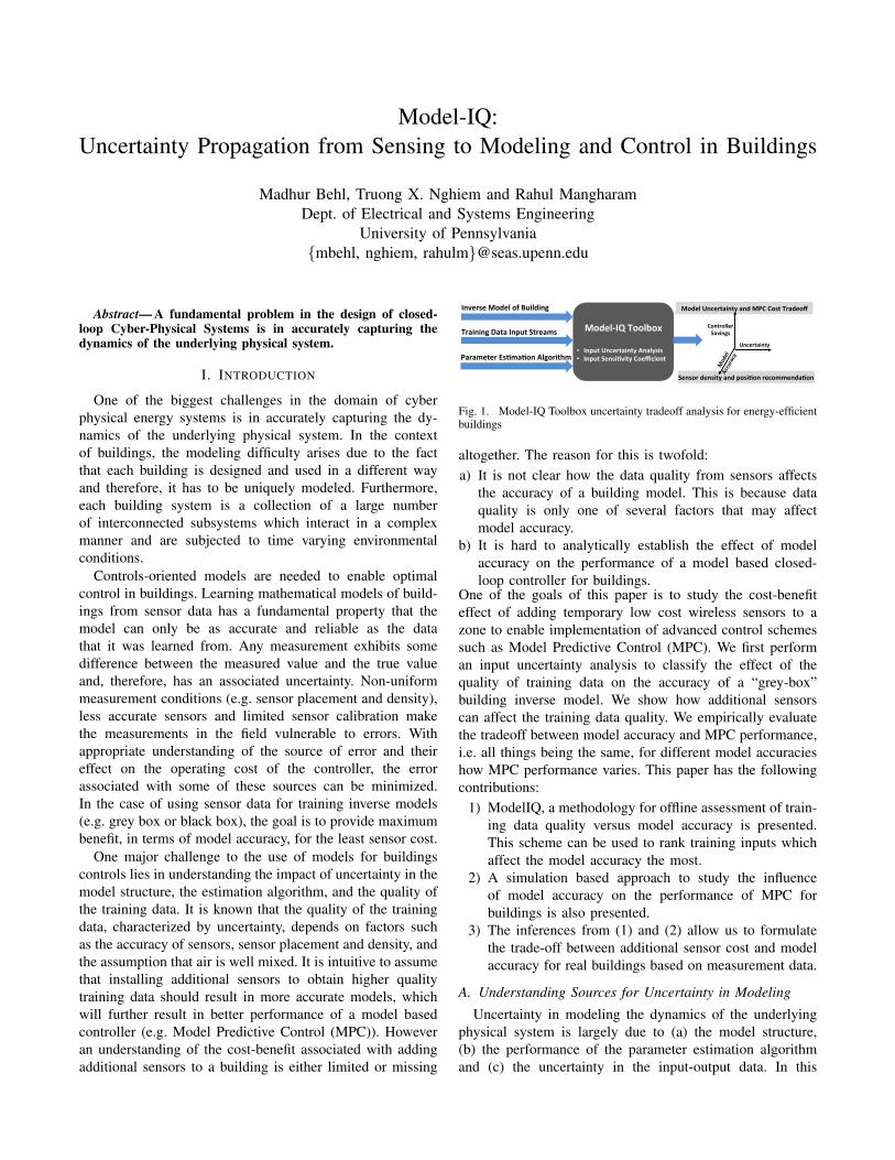
Fig. 1. Model-IQ Toolbox uncertainty tradeoff analysis for energy-efficientbuildings
altogether. The reason for this is twofold:a) It is not clear how the data quality from sensors affects
the accuracy of a building model. This is because dataquality is only one of several factors that may affectmodel accuracy.
b) It is hard to analytically establish the effect of modelaccuracy on the performance of a model based closed-loop controller for buildings.
One of the goals of this paper is to study the cost-benefiteffect of adding temporary low cost wireless sensors to azone to enable implementation of advanced control schemessuch as Model Predictive Control (MPC). We first performan input uncertainty analysis to classify the effect of thequality of training data on the accuracy of a “grey-box”building inverse model. We show how additional sensorscan affect the training data quality. We empirically evaluatethe tradeoff between model accuracy and MPC performance,i.e. all things being the same, for different model accuracieshow MPC performance varies. This paper has the followingcontributions:
1) ModelIQ, a methodology for offline assessment of train-ing data quality versus model accuracy is presented.This scheme can be used to rank training inputs whichaffect the model accuracy the most.
2) A simulation based approach to study the influenceof model accuracy on the performance of MPC forbuildings is also presented.
3) The inferences from (1) and (2) allow us to formulatethe trade-off between additional sensor cost and modelaccuracy for real buildings based on measurement data.
A. Understanding Sources for Uncertainty in Modeling
Uncertainty in modeling the dynamics of the underlyingphysical system is largely due to (a) the model structure,(b) the performance of the parameter estimation algorithmand (c) the uncertainty in the input-output data. In this

effort, we assume the first two are fixed as there are well-established inverse models for buildings. Our focus is thus onunderstanding the effect of uncertainty of the training datafrom the building and environment sensors on the overallcost of operating a model-based controller for the buildingsHVAC systems.
The uncertainty in training data can be characterized intwo ways: bias error or measurement noise (i.e. randomerror). Biases are essentially offsets in the observations formthe true value. Bias error can also be referred to as thesystematic error, precision or fixed error. The bias in thesensor measurement is due to a combination of two reasons.The first reason is the sensor precision. The best correctiveaction in this case is to ascertain the extent of the bias(using the data-sheet or by re-calibration) and to correctthe observations accordingly. The sensor may also exhibitbias due to its placement, especially if it is measuring aphysical quantity which has a spatial distribution, e.g. airtemperature in a zone. In this case, it is hard to detector estimate the bias unless additional spatially distributedmeasurements are obtained. Random error is an error due tothe unpredictable and unknown extraneous conditions thatcan cause the sensor reading to take some random valuesdistributed about a mean. Furthermore, random errors can beadditive or multiplicative. Additive errors are independent ofthe magnitude of the observation while multiplicative errordepend on the magnitude of the observation.
In buildings, the density and location of sensors in a zoneeffects the deviation of the measured temperature value fromthe true temperature value. For instance, a temperature sensorplaced too close to the wall, window, supply or return air ductcan introduce a bias in the sensor measurement. As we willsee in the next section, a bias in the zone temperature valuecan lead to wastage of energy and discomfort with simplezone air control schemes like On-Off and PID control.
B. A Simple Example of Uncertainty Propagation
In this example we examine how underestimating or over-estimating the temperature of a zone can directly affect theenergy consumption and comfort levels in a zone. Considerthe case of controlling a heater in a single zone house asshown in Fig 2. The set point of the temperature inside thezone is fixed at 21◦C. Due to the low temperature (averagevalue 8◦C) outside the house the heater has to constantlywork to maintain the zone temperature at the set-point.
ThermostatSet Point
21
Sensor Bias
0
PlotResults
1/s
House
Heater
On/Off
TroomHeatFlow
Daily TempVariation
Cost Calculator
cost
Avg OutdoorTemp
8
blowercmdTerr
Tindoors
Toutdoors Temperatures
HeatCost
Fig. 2. Thermal model of a house with on-off control
We consider two different control strategies for the heater:On-Off control and PID control, which are widely use dinexisting buildings. In On-Off control the thermostat switchesthe heater on or off while ensuring that the temperature in thezone always remains within ±2◦ of the set-point temperature.This simple control scheme is also referred to as 2-setthermostat control. In the second case, the PID controllerdirectly controls the supply air temperature and flow into thezone in order to always maintain the set point temperature.The simulation period is run for 48h and the cost of energyis fixed at 15c per kW h. The baseline scenario is the casewhen there is no sensor bias in the zone temperature value.In this case the mean zone temperature for the duration of thesimulation is always the same as the set point temperatureof 21◦C for both On-Off and PID control. For the baselinecase, the total energy cost for On-Off control is $36.41 and$36.33 for the PID case. The costs are nearly identical sincethe mean value of the zone temperatures are nearly the samein both cases.
In both the cases we deliberately introduce a fixed sensorbias and evaluate the zone output in terms of comfort andcost of energy. Let us assume that the bias occurs dueto incorrect placement of the temperature sensor. Figure 3shows the comparison of the zone temperature for differentbias values for the two different control schemes. It alsoshows the change in the energy cost of the zone fromthe baseline cost for different values of the sensor bias.When the sensor underestimates the zone temperature bysome bias value (say −3◦C) the mean temperature of thezone increases by the same bias and causes the zone tooverheat i.e. the mean zone temperature goes up to 24◦Cfrom 21◦C. This causes the heating system to consume moreenergy as it needs to compensate for the underestimated zonetemperature. On the other hand, if there is a positive sensorbias (say +3◦C) then it causes the mean value to decreaseby the amount of bias and results in a lower and muchcooler zone temperature i.e. mean zone temperature dropsfrom 21◦C to 18◦C. Although, the energy consumption forthis case is less, it is only at a the cost of zone comfort.The change in energy cost is the same for both the controlschemes. This is because the mean temperature of the zonefor all values of the sensor bias is very similar for both thecases and hence they consume almost the same amount oftotal energy.
Therefore, a bias in the temperature measurement of thezone ( due to the location and density of temperature sensors)affects the zone comfort and energy consumption. However,note that both the controllers are model-independent i.e. theyonly used the measurement of the process variable (whichis the room temperature in this case) to compute the controlsignal that will either track the set-point (PID) or keep thetemperature bounded around the set-point (On-Off). As weproceed to apply model based control schemes for buildingretrofits, the bias or the uncertainty in the measured data willalso influence the accuracy of the model itself which in turnaffects the performance of the model based controller, whichis the focus of this paper.

0 5 10 15 20 25 30 35 40 45 5015
20
25
time(hr)
Tem
p(C
)Temperature vs Time
No Bias+3-3
0 5 10 15 20 25 30 35 40 45 5016
18
20
22
24
time(hr)
Tem
p(C
)
Temperature vs Time
No Bias +1+2 +3-1 -2-3
+3 +2 +1 No Bias -1 -2 -3
−20
0
20
Sensor Bias
Chan
gefrom
baseline Bias vs Energy Consumption
Fig. 3. The zone temperature for the simulation period is plotted fordifferent temperature sensor bias values for: (a) On-Off control, and (b)PID control. (c) shows the change in the energy cost of the zone from itsbaseline value for different bias values
Organization: This paper is structured as follows. Webegin with a short primer on the inverse modeling processfor buildings in Section II. The Model-IQ approach forinput uncertainty analysis for inverse models is presented inSection III. In Section IV, we quantify the effect of the modelaccuracy on the performance of a model predictive controller.Section V then presents a data-driven case study in whichwe demonstrate our approach on sensor data obtained from areal building. Section VI presents the result of an experimentto understand the relationship between the quality of dataand the location of the sensor. Section IX follows the relatedwork and concludes the paper with a discussion on the useof the free and open-source Model-IQ toolbox.
II. INVERSE MODELING
The main objective of an HVAC system for air temperaturecontrol is to reject disturbances due to outside weather con-dition and internal heat gain caused by occupants, lightingand plug-in appliances. Therefore, the building model mustaccurately capture the thermal response of the building tothe different disturbances.
Building models can be broadly classified into three cate-gories:
1) White-box models are based on the laws of physicsand permit accurate and microscopic modeling of thebuilding system. High fidelity building simulation pro-grams like EnergyPlus and TRNSYS ♥1 fall into thiscategory. Although such models provide a high degreeof accuracy they are unsuitable for control design dueto their high level of complexity. These models use alarge number of parameters which must be obtainedfrom a detailed description of the building. Furthermore,
1RAHUL: Need citations
the process of constructing the model and tuning theparameters with limited data is very time consumingand not cost effective.
2) Black-box models are not based on physical behaviors ofthe system but rely on the available data to identify themodel structure. These models are often purely statisti-cal and have a simple structure (e.g. linear regression).However, they provide little insight into the dynamicsdictating the system behavior.
3) Grey-box models fall in between the two above cate-gories. A simplified model structure is chosen looselybased on the physics of the underlying system and theavailable data is used to estimate the values of the modelparameters. These models are suitable for control designand still respect the physics of the system.
A. Model Structure
While there are several methods available for modelingthe dynamics of a building, in this paper we will focus onthe analysis of only grey-box RC models. A commonly usedgrey-box representation of the thermal response of a buildingdue to heat disturbances uses a lumped parameter Resistive-Capacitative (RC) network. This approach for modelingbuildings has been used widely, e.g. in [1], [2], [3]. Figure 4shows an example of such a model for a single zone, as usedin [1]. In this representation, the central node of the RC net-work represents the zone temperature Tz(◦C). The geometryof the zone is divided into different kinds of surfaces, eachof which is modeled using a ’lumped-parameter’ branch ofthe network. For instance, all the external walls of the zoneare lumped into a single wall with 3R2C (3 resistances and 2capacitance) parameters. The same process is applied to theceiling, the floor and the internal (or adjacent) walls of thezone. The zone is subject to several (heat) disturbances whichare applied at different nodes in the network in the followingmanner: (a) solar irradiation on the external wall Qsol,e(W)and the ceiling Qsol,c(W) is applied on the exterior nodeof the lumped wall. (b) incident solar radiation transmittedthrough the windows Qsolt(W) is assumed to be absorbedby the internal and adjacent walls, (c) radiative internal heatgain Qrad(W) which is distributed with an even flux tothe walls and the ceiling, (d) the convective internal heatgain Qconv(W) and the sensible cooling rate Qsens(W) isapplied directly to the zone air, (e) The zone is also subject toheat gains due to the ambient temperature Tamb(◦C), groundtemperature Tg(◦C) and temperatures in other zones whichare accounted for by adding boundary condition nodes toeach branch of the network. The list of all parameters in themodel and their descriptions is given in Table I.
Given this model, the nodal equations for the lumped

Fig. 4. RC lumped-parameter model representation for a thermal zone
external wall and the ceiling network are:
CeoTeo(t) = Ueo(Ta − Teo(t)) + Uew(Tei(t)− Teo(t)) + Qsol,e(1a)
CeiTei(t) = Uew(Teo(t)− Tei(t)) + Uei(Tz(t)− Tei(t)) + Qrad,e(1b)
CcoTco(t) = Uco(Ta − Tco(t)) + Ucw(Tci(t)− Tco(t)) + Qsol,c(1c)
CciTci(t) = Ucw(Tco(t)− Tci(t)) + Uci(Tz(t)− Tci(t)) + Qrad,c(1d)
Similarly, one can write the equations for the dynamics ofthe nodes of the floor and internal wall network. The law ofconservation of energy gives us the following heat balanceequation for zone
CzTz(t) = Uei(Tei(t)− Tz(t)) + Uci(Tci(t)− Tz(t))+ Uii(Tii(t)− Tz(t)) + Ugi(Tgi(t)− Tz(t))
+ Uwin(Ta(t)− Tz(t)) + Qconv + Qsens (2)
Differential equations (1a) to (1d) and (2) can be combinedto give the state space model of the system:
x(t) = Ax(t) +Bu(t)
y(t) = Cx(t) +Du(t)(3)
where the state x is a vector of all node temperatures ofthe model, i.e. x = [Teo, Tei, Tco, Tci, Tgo, Tgi, Tio, Tii, Tz]
T .The input u is a vector of all the inputs to the systems, i.e.u = [Ta, Tg, Ti, Qsol,e, Qsol,c, Qrad,e, Qrad,c, Qrad,g, Qsolt,Qconv, Qsens]
T . The control input to the zone is the sensiblecooling rate Qsens. The cooling rate can be controlled bychanging the mass flow rate of cold air which enters thezone (in case of cooling) or by changing the set point of thesupply air temperature. The rest of the inputs are disturbancesto the zone. The elements of the state matrix A and the inputmatrix B depend non-linearly on the U and C parameters ofthe model. Let us consider θ = [Ueo, Uew, Uei, . . . Cio, Cii]
T ,as a vector of all the parameters of the model Then thestate space equations have the following representation which
TABLE ILIST OF PARAMETERS
U?o convection coefficient between the wall and outside airU?w conduction coefficient of the wallU?i convection coefficient between the wall and zone airUwin conduction coefficient of the windowC?? thermal capacitance of the wallCz thermal capacity of zone zig floore external wallc ceilingi internal wall
emphasizes the parameterization of the A, B, C and Dmatrices.
x(t) = Aθx(t) +Bθu(t)
y(t) = Cθx(t) +Dθu(t)(4)
The entries of output matrix C and the feed-forward matrixD depend on the output of interest. For instance, if theoutput of the model is the zone temperature then C =[0, 0, . . . , 0, 1], which is a row vector with all entries equalto zero except the last entry corresponding to the zonetemperature Tz equal to one. In this case D = 0, the nullmatrix. The model structure is based on the underlyingassumption that the air inside the zone is well mixed andthus, it can be represented by a single node. Furthermore,only one dimensional heat transfer is assumed for the wallsand there is no lateral temperature difference. The parametersof the model are assumed to be time invariant.
B. Parameter Estimation (Model Training)
We first consider the discrete-time state space representa-tion of the dynamical system of Eq. (4)
x(k + 1) = Aθx(k) +Bθu(k)
y(k) = Cθx(k) +Dθu(k)(5)
The goal of parameter estimation is to obtain estimatesof the parameter vector θ of the model from input-outputtime series measurement data. The parameter search spaceis constrained both above and below by θl ≤ θ ≤ θu. For agiven parameter set θ, the model, given by Eq. (5), can be
used to generate a time series of the zone air temperatureTzθ using the measured time series data for the inputs u(t).The subscript θ denotes that the temperature value Tzθ isthe predicted value using the model with parameters θ andthe inputs u. This model generated time series Tzθ may thenbe compared with the corresponding observed values of thezone temperature Tzm , and the difference between the two isquantified by a statistical metric. The metric usually chosenis the sum of the squares of the differences between the twotime series. The parameter estimation problem is to find theparameters θ∗, subject to θl ≤ θ ≤ θu, which result in theleast square error between the predicted and the measuredtemperature values, i.e.
minθ∗
J =
N∑i=1
(Tzm(i)− Tzθ (i))2 (6)
where the summation is over the N data points of the input-output time series under investigation.
The least square optimization of Eq. (6) is a constrainedminimization of a non-linear objective. It is numericallysolved using a trust region reflective algorithm [4] suchas the Levenberg-Marquardt [5] algorithm. A well knownproblem with non-linear search algorithms is the problem ofthe solution getting stuck at a local minima. For this reason,it is required that the initial parameter estimates θ0 shouldbe as close as practicable to their (unknown) optimal (true)values. Generally speaking, the further the initial guess aboutthe parameters values is away from the true values, the biggerthe search region is for the optimization. As search regiongrows, it becomes more likely that the estimation processwill converge to a local optimum.
III. MODELIQ
In this section, we describe the ModelIQ approach for an-alyzing uncertainty propagation for building inverse models.We describe the methodology through an elaborated casestudy.
The accuracy of the building inverse model depends pri-marily on the following three factors:(a) The structure of the model which depends on the extent
to which the model respects the physics of the underlyingphysical system,
(b) The performance of the estimation algorithm. Asdiscussed previously, in the case of non-linear estimationthe performance of the algorithm depends heavily on thenominal values of the parameters, and
(c) The quality of the training data, which can be char-acterized by its uncertainty.
The main premise of the input uncertainty propagation isthat once the model structure and the parameter algorithmare fixed, one can study the influence of the uncertaintyin the training data on the accuracy of the model usingvirtual simulations which utilize artificial data-sets. For theremaining part of the section we describe the results ofconducting the input uncertainty propagation analysis for avirtual building modeled in TRNSYS.
3,600 3,700 3,800 3,900 4,000 4,100 4,200 4,300 4,40014
14.5
15
15.5
16
C
Ground Temeprature
3,600 3,700 3,800 3,900 4,000 4,100 4,200 4,300 4,4000
10
20
30
40
C
Ambient temperature
3,600 3,700 3,800 3,900 4,000 4,100 4,200 4,300 4,4000
0.5
1
1.5
2·104
W
External Solar Irradiation
3,600 3,700 3,800 3,900 4,000 4,100 4,200 4,300 4,4000
1,000
2,000
3,000
4,000
W
Transmitted Solar Irradiation
3,600 3,700 3,800 3,900 4,000 4,100 4,200 4,300 4,4000
1,000
2,000
3,000
4,000
W
Convective Heat Gain
3,600 3,700 3,800 3,900 4,000 4,100 4,200 4,300 4,4000
500
1,000
1,500
2,000W
Radiative Heat Gain
3,600 3,700 3,800 3,900 4,000 4,100 4,200 4,300 4,4000
1,000
2,000
3,000
4,000
June (time in hours)
W
Sensible Cooling Rate
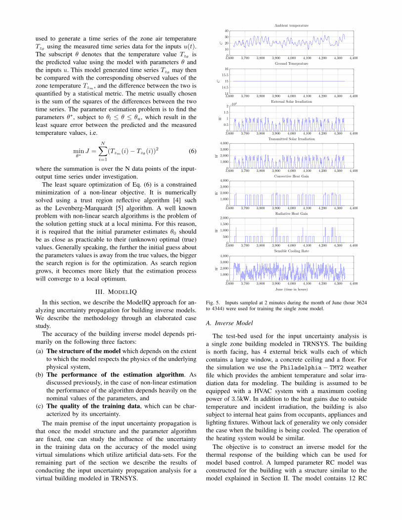
Fig. 5. Inputs sampled at 2 minutes during the month of June (hour 3624to 4344) were used for training the single zone model.
A. Inverse Model
The test-bed used for the input uncertainty analysis isa single zone building modeled in TRNSYS. The buildingis north facing, has 4 external brick walls each of whichcontains a large window, a concrete ceiling and a floor. Forthe simulation we use the Philadelphia− TMY2 weatherfile which provides the ambient temperature and solar irra-diation data for modeling. The building is assumed to beequipped with a HVAC system with a maximum coolingpower of 3.5kW. In addition to the heat gains due to outsidetemperature and incident irradiation, the building is alsosubject to internal heat gains from occupants, appliances andlighting fixtures. Without lack of generality we only considerthe case when the building is being cooled. The operation ofthe heating system would be similar.
The objective is to construct an inverse model for thethermal response of the building which can be used formodel based control. A lumped parameter RC model wasconstructed for the building with a structure similar to themodel explained in Section II. The model contains 12 RC

3,600 3,700 3,800 3,900 4,000 4,100 4,200 4,300 4,400
15
20
25
30
June (time in hours)
ZoneTem
eprature
◦C
Training Error
PredictedActual
(a)
4,340 4,360 4,380 4,400 4,420 4,440 4,460 4,480 4,500 4,520
15
20
25
30
First week of July (time in hours)
ZoneTem
eprature
◦C
Testing Error
PredictedActual
(b)
Fig. 6. The fit between the predicted and actual values of the zonetemperature for the training period (June) is shown in (a) while, (b) showsthe fit between the predicted and actual zone temperature values for thetesting period which was the first week of July
parameters which need to be estimated. The inverse modelcontains a total of seven inputs and an output. The sixdisturbance inputs are: the ambient temperature (Ta), theground temperature (Tg), the external incident solar irradi-ation (Qsole), the solar irradiation transmitted through thewindows (Qsoltr), radiative heat gain (Qgrad) and convectiveinternal heat gain (Qconv). The output of the inverse modelis the temperature of the zone while the control input isthe sensible cooling rate (Qsen). The training data for themodel is in the form of time-series data for each of theinputs and the output. The training period is the month ofJune (hours 3624-4344 in TRNSYS). The input-output time-series data is generated at a sampling rate of 2 minutes forthe entire training period. All the different training inputsused for inverse modeling are shown in Fig. 5.
For this case study, the nominal values of the RC parame-ters of the model were estimated from the construction detailsof the building, obtained from TRNSYS. Fig. 6(a) showsthe result of non-linear parameter estimation problem (6) forthe training period. The result of the inverse model trainingare estimates of the RC parameters, and hence the matricesA,B,C and D of the state-space model. The comparisonbetween the predicted zone temperature values from themodel and the actual zone temperature is shown. The rootmean square error (RMSE) of the fit was 0.187 and theR2 value is 0.971. The R2 coefficient of determination isa statistical measure of the goodness of fit of a model.Its value lies between [0, 1] with a value of 1 indicatingthat the model perfectly fits the data. The R2 coefficientalso indicates how much of the variance of the data can bedescribed by the model. However, measuring the fit statisticson the training period alone is never sufficient, since themodel may be over-fitting the data. Therefore, the accuracyof the inverse model was also tested on a test data set. Thetest data set corresponds to the first week of July (hours
4344-4512 in TRNSYS). The time-series of inputs for thetest period were used with the learned model and the resultsof the comparison between the predicted model output andthe actual zone temperature is shown in Fig. 6(b). The RMSEfor the testing period was 0.292 with a R2 value of 0.961.These stats are a better indicator of the accuracy of the modelsince during the testing period the model is subject to aninput data-set that it was not trained on.
B. Input Uncertainty Analysis
The aim of this analysis is to determine the influence of theuncertainty (bias) in the training data inputs on the accuracyof the inverse model and then, to quantify the relativeimportance of the inputs. First, some notation is introducedfor brevity. We consider a model with m > 0 training inputdata sets denoted by U = {u1, · · · , um}. Note that these areinputs for model training, not the inputs for the model itself,e.g. even though zone temperature is a model output, it isstill a required data-set (hence, an input) for model training.Ui,δ = {ui = ui + δ, uj = uj |i, j ≤ m, j 6= i} denotes theartificial data-set obtained by perturbing input ui by anamount δ while keeping all other inputs data sets unper-turbed. U0 denotes the data-set in which all the inputs areunperturbed. Now, MUi,δ is the inverse model with obtainedby training on the data-set Ui,δ and MU0 is the modelobtained by training on a completely unperturbed data-set.We denote the RMSE of the model MUi,δk
by r(MUi,δk).
The ModelIQ approach for conducting an input uncertaintyanalysis consists of the following steps:(a) Establish a baseline (reference) model: The baseline
model, MU0, is the inverse model obtained by training
on the unperturbed data set U0, which is considered asthe ground truth.
(b) Determine which model outputs will be investigated fortheir accuracy and what are their practical implications.
(c) Each of the input data streams are then perturbed withinsome bounds. There are a total of N perturbationsδ1, · · · , δN for each input stream ui, i ≤ m. This resultsin N artificial data-sets Ui,δ1 , · · · , Ui,δN for each inputstream i.
(d) Corresponding to every perturbation, the inverse mod-eling process is run again and a new model MUi,δk
isobtained.
(e) The prediction accuracy of each of the trained modelis evaluated on a common input data stream UT . Theaccuracy of the model MUi,δk
is measured by the RMSEr(MUi,δk
) between the predicted and the actual modeloutput values for the common input stream UT .
(f) Using the RMSE of the fit and the magnitude of theperturbation, determine the sensitivity coefficient (orinfluence coefficient) for each input training stream.
An overview of the steps for the input uncertainty analysisis shown in Fig. 8.
For our case study, the baseline model is the model trainedon unperturbed training data-set i.e. the original input data-set corresponding to the month of June. The RMSE for the

−20 −15 −10 −5 0 5 10 15 20
0
50
100
150
200
250
300
350
400
Percentage of input perturbationNormalized
percentagechange
inmodelaccuracy
Ambient Temperature
(a)
−20 −15 −10 −5 0 5 10 15 20
0
20
40
60
80
100
120
140
Percentage of input perturbation
Normalized
percentagechange
inmodelaccuracy
External Solar irradiance
(b)
−20 −15 −10 −5 0 5 10 15 20
0
10
20
30
40
50
60
Percentage of input perturbation
Normalized
percentagechange
inmodelaccuracy
Radiative Heat Gain
(c)
−20 −15 −10 −5 0 5 10 15 20
0
50
100
150
200
250
300
Percentage of input perturbation
Normalized
percentagechange
inmodelaccuracy
Convective Heat Gain
(d)
−20 −15 −10 −5 0 5 10 15 200
100
200
300
400
500
600
700
800
Percentage of input perturbation
Normalized
percentagechange
inmodelaccuracy
Sensible Cooling Load
(e)
−20 −15 −10 −5 0 5 10 15 20
0
50
100
150
200
250
300
350
Percentage of input perturbation
Normalized
percentagechange
inmodelaccuracy
Transmitted solar irradiation
(f)
−20 −15 −10 −5 0 5 10 15 20−5
0
5
10
15
20
25
30
35
40
Percentage of input perturbation
Normalized
percentagechange
inmodelaccuracy
Ground Temperature
(g)
Fig. 7. Input uncertainty analysis results for a single zone TRNSYS model. The x axis shows the magnitude of the perturbation in percent change fromthe unperturbed data while the y axis is the percent change in the model accuracy compared to the RMSE for the model trained on unperturbed data. Thefollowing inputs are shown: (a) ambient temperature (◦C); (b) incident solar irradiation on the external walls (W); (c) radiative internal heat gain (W);(d) convective internal heat gain (W); (e) sensible cooling rate (W); (f) solar irradiation transmitted through the windows (W); and, (g) floor (ground)temperature (◦C).
Parameter
Estimation
(Inverse
Model
Training)
Prediction
Error
Perturb
each input
stream(N perturbations)
Common
input for
evaluation
Different parameters
estimated for each
perturbation(N models)
(N different fits)
...
...
Input Data Stream
Sensible Cooling
Convective Gain
External Solar
Radiative gain
Transmitted Solar
Ambient temp.
Ground temp.
Fig. 8. Overview of the ModelIQ input uncertainty analysis methodology,an offline method to confirm the influence of each training input on theaccuracy of the model.
baseline model is denoted by r(MU0). The artificial data-
sets are created in a normalized manner by adding (andsubtracting) a bounded and fixed bias to the unperturbeddata in the form of the per-cent change from the unperturbed(baseline) value i.e. the perturbations δk’s are in form of per-cent changes around the unperturbed data point. Therefore,each data-point xi belonging to the unperturbed input uigets perturbed to a new value of xi = xi(1 + δk/100).This is done so that every input is treated in the samemanner regardless of the scale of the input. One can relatethe per-cent change to the absolute value of the change,simply through the mean of the data-set. For e.g. if themean of unperturbed ambient temperature was 20◦C, thenthe mean of data which was perturbed δ = +10% wouldbe 22◦C which is equivalent to a mean absolute bias of 2◦
degrees in the ambient temperature. Each of the 7 traininginput data streams (Fig. 8) are perturbed one at a timewithin [−20%, 20%] around the unperturbed nominal valuewith increments of 1%. Every perturbation for each of theinputs creates an artificial training set for the inverse model.Therefore for each of the 7 input streams, N = 40 additional
artificial data-sets Ui,δ1 , ·, Ui,δ40 were created resulting in atotal 280 different training data-sets. The inverse model forthe single zone building was trained on each of the artificialdata-set and the accuracy of the model was evaluated in termsof the RMSE on the test data-set. The use of a common testdata-set for evaluating the accuracy of the model ensures afairness in the comparison of the influence of the uncertaintyamong different inputs on the model accuracy.
Finally the model accuracy sensitivity coefficient is calcu-lated as follows:
γi = Mean(k=1,··· ,N)
(r(MUi,δk
)− r(MU0)/r(MU0
)
|δk|
)(7)
It is the mean of the ratio of the normalized change in themodel accuracy to that of the normalized change in the mag-nitude of the input data stream. Both normalization’s are withrespect to the baseline case. The magnitude of the sensitivitycoefficient γi can be interpreted as the mean value of thechange in the RMSE of the model due to 1% bias uncertaintyin the training data stream i. The sensitivity coefficient issometimes also referred to as the influence coefficient orpoint elasticity. The results for the input uncertainty analysisfor the TRNSYS building are shown in Fig. 7. These resultsalign well with the intuition that as the magnitude of theuncertainty bias increases in the input data stream the inversemodel becomes worse and its prediction error increases. Thisis the case for all the input data streams and it results in theparabolic trend. The shape of the curve varies from input toinput, due to a different sensitivity coefficient value, and is an

Qsen Ta Qsoltr Qconv Qsole Qgrad Tg0
10
20
30
Inputs
Model
Acc
ura
cySen
siti
vit
yC
oeffi
cien
t
Fig. 9. Comparison of model sensitivity coefficients for the different inputtraining data streams.
indicator of the extend to which a particular input influencesthe model accuracy.
The model accuracy sensitivity coefficients were calcu-lated for every input data stream and their comparison isshown in Fig. 9. For the building under consideration, itis clear that the sensible cooling rate, ambient temperature,transmitted solar gain and convective heat gains shouldbe measured accurately in order to learn a good inversemodel. Note that, although the results presented in this paperassume a particular building and a fixed model structure, theModelIQ approach itself is a general approach which can beused to identify the inputs which should be measured moreaccurately in order to obtain accurate building models.
IV. MODEL ACCURACY VS MPC PERFORMANCE
While the input uncertainty analysis reveals importantinsights about the relationship between data quality andmodel accuracy, it is not clear how much of an impactdoes model accuracy have on the performance of a modelbased building controller. Therefore, it is also necessary toexamine if the model accuracy can have any direct economicimpact. Especially when energy-efficient control algorithmsrely on the accuracy of the underlying mathematical modelof the building in order to figure out optimal control inputs.Installation of additional sensors in a building can yieldbetter quality of data for model training but there is a trade-off between how good can an inverse model can performversus how much cost is spent on obtaining the inversemodel. These trade-offs can be better understood if anend-to-end relationship between the data uncertainty, modelaccuracy and control cost are known. There is significantvalue in knowing how much the cost of a model predictivecontroller changes with changes in the model accuracy. Thisinformation can be used to provide ”target” accuracy levelsfor the inverse model, which in turn specify the degree ofaccuracy required on the sensing.
However, it is a hard problem to analytically determine theimpact of the model accuracy on the MPC performance. Theproblem arises due to the complexity of the model structureand the MPC formulation itself. For this reason, to quantifythe effect of model accuracy on the performance of a MPCcontroller we make use of an empirical analysis with thesame single zone TRNSYS model used in section III. First,a model predictive controller was designed for the zone.The MPC simulation is then ran for models of different
t t+ 1 t+N
u(t)
u(t+ 1)u(t+N − 1)
applied
moving windowfuturepast
Fig. 10. Finite-horizon moving window of MPC: at time t, the MPCoptimization problem is solved for a finite length window of N steps andthe first control input u(t) is applied; the window then recedes one stepforward and the process is repeated at time t+ 1.
accuracy and the outputs are compared to reveal the trendof model accuracy vs MPC cost. We now describe the MPCformulation followed by the results of this analysis.
A. MPC formualtion
The MPC problem involves optimizing a cost functionsubject to the dynamics of the system, over a finite horizonof time. Based on the cost function and the constraints on thezone temperature, the MPC controller calculates a sequenceof control inputs which minimize the cost for the length ofthe finite horizon. The first computed input is applied, andat the next step the optimization is solved again as shown inFigure 10.
The state-space model zone model in eq (5) can also bewritten as follows:
x(k + 1) = Ax(k) +Bu(k) + Ed(k) (8a)y(k) = Cx(k) (8b)
Where the cooling rate to the zone is the control input u(k)and d(k) is the vector of all the disturbances into the zone(ambient temperature, heat gains etc).
To reduce the number of control variables we use themove-blocking technique. During each move-blocking win-dow of length l, the control u is held constant. So u(0) =u(1) = · · · = u(l − 1), u(l) = u(l + 1) = · · · = u(2l − 1)and in general u(il) = u(il+ 1) = · · · = u((i+ 1)l− 1) i.e.MPC re-optimizes at integral multiples of the window lengthil only.
Let us consider a control horizon H in terms of move-blocking windows, so the number of time steps is Hl. Attime t = il, the MPC problem is to minimize
H−1∑k=0
t+(k+1)l−1∑σ=t+kl
(PU (σ)u(k) + PT (σ) (y(σ − ysp(σ))
2)

subject to
x(t) = x0 cx(t+ kl + 1)...
x(t+ (k + 1)l)
= diag(A)
cx(t+ kl)...
x(t+ (k + 1)l − 1)
+ col(B)u(k) + diag(E)
cd(t+ kl)...
d(t+ (k + 1)l − 1)
umin(σ) ≤ u(k) ≤ umax(σ)
where the last two constraints hold for all k = 0, . . . ,H − 1and σ = t+kl, . . . , t+(k+1)l−1, diag(·) represents a blockdiagonal matrix of appropriate dimensions, and col(B) is thecolumn vector constructed by stacking the columns of matrixB. PU (σ) is the price of electricity at time σ and PT (σ) isthe penalty for errors in tracking the desired zone temperaturetrajectory ysp(σ). Both the cost and penalty functions varythroughout the day, for example the price of electricity can behigh during the peak hours of the day as compared to the offpeak hours. Similarly, the set-point temperature can changeduring the day depending on the zone occupancy. Note thatin our MPC formulation we only consider soft constraints onthe zone temperature. The initial state of the system is x0,while umin(σ) and umax(σ) are the lower and upper boundson the cooling rate u(k) which can vary during the day toaccount for equipment schedules.
B. State Observer
In order for us to use the state space model (5) for modelpredictive control, we also need to design a state observer.The state observer is designed to provide the estimates ofx(k|k), the state of the plant model at every MPC timestep. The estimates are computed from the measured outputym(k) by the linear state observer. The reason for estimatingthe states of the plant is that the states x1, · · · , xn−1 arelumped parameter temperatures which are hard (and almostimpossible) to measure.
Given the discrete plant model
x(k + 1) = Ax(k) +Bu(k) +Gw(k)
y(k) = Cx(k) +Du(k) +Hw(k) + v(k)
where, w(k) is white process noise and v(k) is white mea-surement noise satisfying E(w(k)) = E(v) = 0, E(wwT ) =Q, E(vvT ) = R, E(wvT ) = N . The estimator has thefollowing state equation:
x(k + 1|k) = Ax(n|n− 1) +Bu(k)
+ L(y(k)− Cx(k|k − 1)) (9)
The gain matrix L is derived by solving a discrete Riccatiequation:
L = (APCT + N)(CPCT + R)−1 (10)
where,
R = R+HN +NTHT +HQHT (11)
N = G(QHT +N) (12)
The prediction x(k|k−1) is updated using the new measure-ment y(k) as:
x(k|k) = x(k|k− 1) +M(y(k)−Cx(k|k− 1)−Du(k))
where the innovation gain M is defined as:
M = PCT (CPCT + R)−1
For the simple case, E(wvT ) = N = 0 , Dd = Du = 0,H = 0, and G = B.
C. Single zone example
The MPC control described above was implemented forthe single zone TRNSYS model. The cooling system ofthe building is always switched on during the occupancyperiod from 8 a.m. in the morning to 6 p.m. in the eveningon weekdays and remains off during the weekend. Themaximum and minimum constraints on the cooling rate wereumax = 3500(W) and umin = 0. The set point temperatureof the zone was kept at 24◦C for the occupancy period. Thezone temperature is allowed to float during the weekend. Thesimulation was ran for a part of the first week of July fromhour 4344-4400 in TRNSYS. The building is also subject topeak demand pricing, i.e. the price of electricity is 10 timethe nominal price during the on-peak hours , which are from1 p.m. to 5 p.m.. We compare two different cases. The first isthe comparison of the building operation with and without anMPC controller. Without MPC control, the cooling switcheson at 8 am and then tries to supply exactly the amount ofcooling energy required to keep the temperature at 24 degreesfor the occupancy period. The total energy consumption forthe simulation period is 93.71(kW h). In this case, the powerconsumption of the cooling system remains high even duringthe peak pricing hours resulting in a total cost of 511.83units.
The baseline model for MPC is the model with the bestRMSE (0.187) for the testing data. This is the model whichwas trained on unperturbed data and was also used asthe baseline for the input uncertainty analysis. The move-blocking step of MPC is 5 minutes and the MPC horizonis 2 hours. The performance of the MPC controller with thecase without MPC is shown in figure 11. The MPC controllerrapidly pre-cools the zone just before the peak power pricingperiod begins at 1 p.m. This can be seen in both the coolingrate and the zone temperature plots. As a result of this, theenergy consumption of the building during the peak hoursis reduced and it results in an overall lower energy cost.The total energy consumption for this case was 87.29(kW h)and the total energy cost was reduced to 442.06 units. Sothere is a 13.63% reduction in the energy cost and a 6.85%reduction in the total energy consumption. While the primaryreason for the reduction in cost is the pre-cooling of thezone, another reason for the lower energy consumption is

4,340 4,350 4,360 4,370 4,380 4,390 4,400 4,410 4,420 4,430 4,4400
1,000
2,000
3,000W
Sensible rate comparison
Without MPCMPC
(a)
4,340 4,350 4,360 4,370 4,380 4,390 4,400 4,410 4,420 4,430 4,44020
22
24
26
C
Zone Temperature
Without MPCMPC
(b)
Fig. 11. (a) shows the comparison between the performance of anMPC controller with the default case without MPC. (b) shows the zonetemperature values for both the controllers.
4,340 4,360 4,380 4,400 4,420 4,440 4,460 4,480 4,500 4,520
15
20
25
30
Zon
eTem
eprature
Model Fit on test data
ActualBaselineInaccurate
(a)
4,340 4,350 4,360 4,370 4,380 4,390 4,400 4,410 4,420 4,430 4,4400
1,000
2,000
3,000
W
Sensible rate comparison
No MPCBaseline Model MPCInaccurate Model MPC
(b)
Fig. 12. (a) shows the comparison of the fit on the test data between thebaseline model RMSE 0.187) and an inaccurate model (RMSE 0.538) (b)shows the comparison between the MPC performance of the models.
that because the MPC has soft temperature constraints, thezone temperature is slightly above the set-point temperaturerequiring it to use less cooling energy.
Having implemented MPC for the baseline model (trainedon unperturbed data), we next use models trained on per-turbed data and compare their performance with the baselinecase. This allows us to observe the trend between MPCperformance and model accuracy. An example of such a sim-ulation run is shown in figure 12. The MPC performance ofthe baseline model has been compared with the performanceof a relatively inaccurate model, with a much higher RMSE(0.538) value than the baseline model with RMSE (0.187).It can be seen that an inaccurate model performs poorlycompared with the ”good” baseline case. The total energyconsumption for the inaccurate model was 91.68(kW h)which is about 2.2% less than the baseline case. The totalenergy cost was 492.53 units, which is a reduction of only
0.15 0.2 0.25 0.3 0.35 0.4 0.45 0.5 0.55
5
10
RMSE of Model
%energy
cost
savings
Fig. 13. Change in the performance of the model predictive controller formodels of different accurateness.
(a)
(b)
Fig. 14. 3D view of Building 101, the site chosen for the case study andthe location of suite 210 in the north-wing of the building.
3.77% as compared with the cost reduction of 13.63% forthe baseline model based MPC. Several inverse models withdifferent accurateness, in terms of their testing RMSE, wereran with the MPC controller. The savings achieved by MPCfor the different models is shown in figure 13. The savingsare measured with respect to the case when no MPC wasused. The trend of the plot aligns with intuition and showsthat MPC performance deteriorates as the underlying modelbecomes worse.
We have now seen that models can lose their predictiveperformance if they are trained on uncertain (biased) data.The input uncertainty analysis revealed the extent to whichdifferent inputs are responsible for the accuracy of theinverse model. By empirically, establishing a relationshipbetween model accuracy and MPC performance, one cantake informed decisions about the investment on additionalsensor requirements to improve the data quality. In the nextsection we apply the ModelIQ tool-chain on a model for areal building using real sensor data.
V. CASE STUDY
The ModelIQ approach described in Section III was ap-plied to real sensor data. The site chosen for analysis iscalled Building 101. Building 101, located in the Navy Yardin Philadelphia, is the temporary headquarters of the U.S.Department of Energy’s Energy Efficient Building Hub [6].It is a highly instrumented commercial building and theacquired data is continuously stored and is made availableto Hub researchers. The building is in the shape of a ”T”with three wings (Figure 14(a)), and is comprised of offices,a lunchroom, mechanical spaces, and miscellaneous support
0 100 200 300 400 500 600 700 800 900 1,000 1,100 1,20023
23.5
24
24.5
25
◦C
Ceiling temperature
0 100 200 300 400 500 600 700 800 900 1,000 1,100 1,200
26
28
30
32
34
◦C
Ambient temperature
0 100 200 300 400 500 600 700 800 900 1,000 1,100 1,20020
22
24
◦C
Porch Temperature
0 100 200 300 400 500 600 700 800 900 1,000 1,100 1,20022
22.5
23
23.5
24
◦C
Floor Temeprature
0 100 200 300 400 500 600 700 800 900 1,000 1,100 1,2000
2
4
·104
W
External Solar Irradiation
0 100 200 300 400 500 600 700 800 900 1,000 1,100 1,200100
150
200
250
300
W
Radiative Heat Gain on Floor
0 100 200 300 400 500 600 700 800 900 1,000 1,100 1,2000
500
1,000
1,500
2,000
W
Convective Heat Gain
0 100 200 300 400 500 600 700 800 900 1,000 1,100 1,2000
200
400
600
800
1,000
W
Radiative Heat Gain on Ceiling
0 100 200 300 400 500 600 700 800 900 1,000 1,100 1,2000
0.2
0.4
0.6
0.8
1·104
June (time in hours)
W
Sensible Cooling Rate
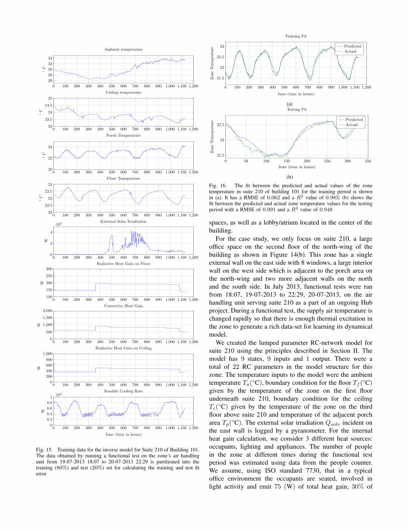
Fig. 15. Training data for the inverse model for Suite 210 of Building 101.The data obtained by running a functional test on the zone’s air handlingunit from 19-07-2013 18:07 to 20-07-2013 22:29 is partitioned into thetraining (80%) and test (20%) set for calculating the training and test fiterror
0 100 200 300 400 500 600 700 800 900 1,000 1,100 1,200
21.5
22
22.5
23
June (time in hours)
Zon
eTem
eprature
Training Fit
PredictedActual
(a)
0 50 100 150 200 250 300 350
21.5
22
22.5
June (time in hours)
Zon
eTem
eprature
Testing Fit
PredictedActual
(b)
Fig. 16. The fit between the predicted and actual values of the zonetemperature in suite 210 of building 101 for the training period is shownin (a). It has a RMSE of 0.062 and a R2 value of 0.983; (b) shows thefit between the predicted and actual zone temperature values for the testingperiod with a RMSE of 0.091 and a R2 value of 0.948
spaces, as well as a lobby/atrium located in the center of thebuilding.
For the case study, we only focus on suite 210, a largeoffice space on the second floor of the north-wing of thebuilding as shown in Figure 14(b). This zone has a singleexternal wall on the east side with 8 windows, a large interiorwall on the west side which is adjacent to the porch area onthe north-wing and two more adjacent walls on the northand the south side. In July 2013, functional tests were ranfrom 18:07, 19-07-2013 to 22:29, 20-07-2013, on the airhandling unit serving suite 210 as a part of an ongoing Hubproject. During a functional test, the supply air temperature ischanged rapidly so that there is enough thermal excitation inthe zone to generate a rich data-set for learning its dynamicalmodel.
We created the lumped parameter RC-network model forsuite 210 using the principles described in Section II. Themodel has 9 states, 9 inputs and 1 output. There were atotal of 22 RC parameters in the model structure for thiszone. The temperature inputs to the model were the ambienttemperature Ta(◦C), boundary condition for the floor Tf (◦C)given by the temperature of the zone on the first floorunderneath suite 210, boundary condition for the ceilingTc(
◦C) given by the temperature of the zone on the thirdfloor above suite 210 and temperature of the adjacent porcharea Tp(◦C). The external solar irradiation Qsole incident onthe east wall is logged by a pyranometer. For the internalheat gain calculation, we consider 3 different heat sources:occupants, lighting and appliances. The number of peoplein the zone at different times during the functional testperiod was estimated using data from the people counter.We assume, using ISO standard 7730, that in a typicaloffice environment the occupants are seated, involved inlight activity and emit 75 (W) of total heat gain, 30% of
−20 −15 −10 −5 0 5 10 15 20−10
−5
0
5
10
15
20
25
30
35
40
45
Percentage of input perturbation
Normalized
percentagechange
inmodelaccuracy
Ambient Temperature
(a)
−20 −15 −10 −5 0 5 10 15 20
0
50
100
150
200
250
300
350
400
450
500
Percentage of input perturbation
Normalized
percentagechange
inmodelaccuracy
Porch Temperature
(b)
−20 −15 −10 −5 0 5 10 15 20
0
20
40
60
80
100
120
140
Percentage of input perturbation
Normalized
percentagechange
inmodelaccuracy
External Solar irradiance
(c)
−20 −15 −10 −5 0 5 10 15 20−10
0
10
20
30
40
50
60
70
Percentage of input perturbation
Normalized
percentagechange
inmodelaccuracy
Radiative Heat Gain on External Wall
(d)
−20 −15 −10 −5 0 5 10 15 20−10
−8
−6
−4
−2
0
2
4
6
8
10
12
Percentage of input perturbation
Normalized
percentagechange
inmodelaccuracy
Radiative Heat Gain on Ceiling
(e)
−20 −15 −10 −5 0 5 10 15 20−10
−8
−6
−4
−2
0
2
4
6
8
10
12
14
16
Percentage of input perturbation
Normalized
percentagechange
inmodelaccuracy
Convective Heat Gain
(f)
−20 −15 −10 −5 0 5 10 15 20
0
50
100
150
200
250
300
350
Percentage of input perturbation
Normalized
percentagechange
inmodelaccuracy
Sensible Cooling Load
(g)
−20 −15 −10 −5 0 5 10 15 20−10
0
10
20
30
40
50
60
Percentage of input perturbationNormalized
percentagechange
inmodelaccuracy
Ground Temperature
(h)
−20 −15 −10 −5 0 5 10 15 20−10
−5
0
5
10
15
20
25
30
35
40
45
Percentage of input perturbation
Normalized
percentagechange
inmodelaccuracy
Ceiling Temperature
(i)
−20 −15 −10 −5 0 5 10 15 200
100
200
300
400
500
600
Percentage of input perturbation
Normalized
percentagechange
inmodelaccuracy
Zone Temeprature
(j)
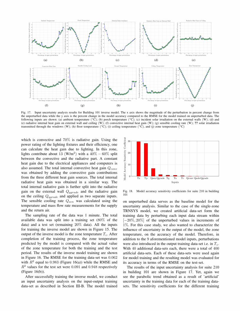
Fig. 17. Input uncertainty analysis results for Building 101 inverse model. The x axis shows the magnitude of the perturbation in percent change fromthe unperturbed data while the y axis is the percent change in the model accuracy compared to the RMSE for the model trained on unperturbed data. Thefollowing inputs are shown: (a) ambient temperature (◦C); (b) porch temperature (◦C); (c) incident solar irradiation on the external walls (W); (d) and(e) radiative internal heat gain on external wall and ceiling (W); (f) convective internal heat gain (W); (g) sensible cooling rate (W); ?? solar irradiationtransmitted through the windows (W); (h) floor temperature (◦C); (i) ceiling temperature (◦C), and (j) zone temperature (◦C)
which is convective and 70% is radiative gain. Using thepower rating of the lighting fixtures and their efficiency, onecan calculate the heat gain due to lighting. In this zone,lights contribute about 13 (W/m2) with a 40% − 60% splitbetween the convective and the radiative part. A constantheat gain due to the electrical appliances and computers isalso assumed. The total internal convective heat gain Qconvwas obtained by adding the convective gain contributionsfrom the three different heat gain sources. The total internalradiative heat gain was obtained in a similar way. Thetotal internal radiative gain is further split into the radiativegain on the external wall Qqgrade and the radiative gainon the ceiling Qqgradc and applied as two separate inputs.The sensible cooling rate Qsen was calculated using thetemperature and mass flow rate measurements for the supplyand the return air.
The sampling rate of the data was 1 minute. The totalavailable data was split into a training set (80% of thedata) and a test set (remaining 20% data). All the inputsfor training the inverse model are shown in Figure 15. Theoutput of the inverse model is the zone temperature Tz . Aftercompletion of the training process, the zone temperaturepredicted by the model is compared with the actual valueof the zone temperature for both the training and the testperiod. The results of the inverse model training are shownin Figure 16. The RMSE for the training data-set was 0.062with R2 equal to 0.983 (Figure 16(a)) while the RMSE andR2 values for the test set were 0.091 and 0.948 respectively(Figure 16(b)).
After successfully training the inverse model, we conductan input uncertainty analysis on the input-output trainingdata-set as described in Section III-B. The model trained
Tz Tp Qsen Qgrade Tg Ta Tc Qconv QsoleQgradc0
10
20
30
Inputs
Model
Acc
ura
cySen
siti
vit
yC
oeffi
cien
t
Fig. 18. Model accuracy sensitivity coefficients for suite 210 in building101
on unperturbed data serves as the baseline model for theuncertainty analysis. Similar to the case of the single-zoneTRNSYS model, we created artificial data-set form thetraining data by perturbing each input data stream within[−20%, 20%] of the unperturbed values in increments of1%. For this case study, we also wanted to characterize theinfluence of uncertainty in the output of the model, the zonetemperature, on the accuracy of the model. Therefore, inaddition to the 9 aforementioned model inputs, perturbationswere also introduced in the output training data-set i.e. in Tz .With 40 additional data-sets each, there were a total of 400artificial data-sets. Each of these data-sets were used againfor model training and the resulting model was evaluated forits accuracy in terms of the RMSE on the test-set.
The results of the input uncertainty analysis for suite 210in building 101 are shown in Figure 17. Yet, again wesee the parabolic trend obtained as a result of ’artificial’uncertainty in the training data for each of the training data-sets. The sensitivity coefficients for the different training
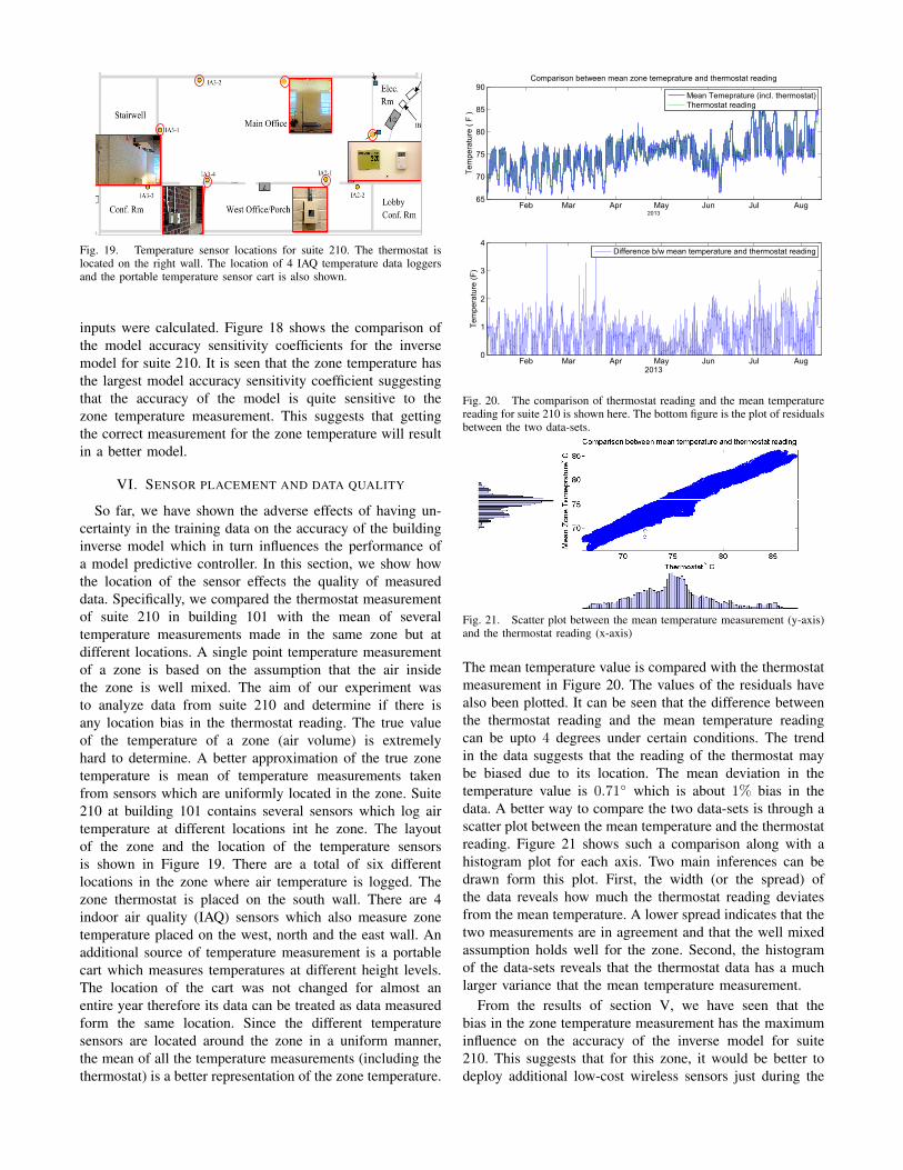
Fig. 19. Temperature sensor locations for suite 210. The thermostat islocated on the right wall. The location of 4 IAQ temperature data loggersand the portable temperature sensor cart is also shown.
inputs were calculated. Figure 18 shows the comparison ofthe model accuracy sensitivity coefficients for the inversemodel for suite 210. It is seen that the zone temperature hasthe largest model accuracy sensitivity coefficient suggestingthat the accuracy of the model is quite sensitive to thezone temperature measurement. This suggests that gettingthe correct measurement for the zone temperature will resultin a better model.
VI. SENSOR PLACEMENT AND DATA QUALITY
So far, we have shown the adverse effects of having un-certainty in the training data on the accuracy of the buildinginverse model which in turn influences the performance ofa model predictive controller. In this section, we show howthe location of the sensor effects the quality of measureddata. Specifically, we compared the thermostat measurementof suite 210 in building 101 with the mean of severaltemperature measurements made in the same zone but atdifferent locations. A single point temperature measurementof a zone is based on the assumption that the air insidethe zone is well mixed. The aim of our experiment wasto analyze data from suite 210 and determine if there isany location bias in the thermostat reading. The true valueof the temperature of a zone (air volume) is extremelyhard to determine. A better approximation of the true zonetemperature is mean of temperature measurements takenfrom sensors which are uniformly located in the zone. Suite210 at building 101 contains several sensors which log airtemperature at different locations int he zone. The layoutof the zone and the location of the temperature sensorsis shown in Figure 19. There are a total of six differentlocations in the zone where air temperature is logged. Thezone thermostat is placed on the south wall. There are 4indoor air quality (IAQ) sensors which also measure zonetemperature placed on the west, north and the east wall. Anadditional source of temperature measurement is a portablecart which measures temperatures at different height levels.The location of the cart was not changed for almost anentire year therefore its data can be treated as data measuredform the same location. Since the different temperaturesensors are located around the zone in a uniform manner,the mean of all the temperature measurements (including thethermostat) is a better representation of the zone temperature.
Feb Mar Apr May Jun Jul Aug65
70
75
80
85
90
2013
Tem
pera
ture
( F
)
Comparison between mean zone temeprature and thermostat reading
Mean Temeprature (incl. thermostat)Thermostat reading
Feb Mar Apr May Jun Jul Aug0
1
2
3
4
2013
Tem
pera
ture
(F)
Difference b/w mean temperature and thermostat reading
Fig. 20. The comparison of thermostat reading and the mean temperaturereading for suite 210 is shown here. The bottom figure is the plot of residualsbetween the two data-sets.
Fig. 21. Scatter plot between the mean temperature measurement (y-axis)and the thermostat reading (x-axis)
The mean temperature value is compared with the thermostatmeasurement in Figure 20. The values of the residuals havealso been plotted. It can be seen that the difference betweenthe thermostat reading and the mean temperature readingcan be upto 4 degrees under certain conditions. The trendin the data suggests that the reading of the thermostat maybe biased due to its location. The mean deviation in thetemperature value is 0.71◦ which is about 1% bias in thedata. A better way to compare the two data-sets is through ascatter plot between the mean temperature and the thermostatreading. Figure 21 shows such a comparison along with ahistogram plot for each axis. Two main inferences can bedrawn form this plot. First, the width (or the spread) ofthe data reveals how much the thermostat reading deviatesfrom the mean temperature. A lower spread indicates that thetwo measurements are in agreement and that the well mixedassumption holds well for the zone. Second, the histogramof the data-sets reveals that the thermostat data has a muchlarger variance that the mean temperature measurement.
From the results of section V, we have seen that thebias in the zone temperature measurement has the maximuminfluence on the accuracy of the inverse model for suite210. This suggests that for this zone, it would be better todeploy additional low-cost wireless sensors just during the

model training phase and get a better estimate of the zonetemperature for training the inverse model. Also, the meanvalue obtained by adding more sensors could be used to re-calibrate or correct the thermostat reading for location bias,resulting in data which can yield an inverse model which canbetter represent the dynamics of the zone.
VII. RELATED WORK
A brief summary of related work in different areas ispresented next.A. MPC related
The treatment and analysis of the implementation of modelbased control schemes like MPC and optimal control forbuildings has been very thorough. Several papers [7], [8], [9]describe the implementation of model predictive control forenergy efficient operation of buildings, supported by strongcase studies. In [10] authors consider uncertainty in theprediction of disturbances and propose a stochastic versionof MPC. In [11], a reduced order model has been used formodel based predictive control. [12] advocates the use sim-pler models for buildings based on the physical descriptionof the bundling. The authors highlight the building modelingprocess as a crucial part for building predictive control.B. Sensitivity analysis related
Parametric sensitivity analysis of a model reveals theimportant parameters of the model which effect the modeloutput the most. [13], [14] among several others are devotedto sensitivity analysis for building modeling. In [13], impor-tant input design parameters are identified and analyzed frompoints of view of annual building energy consumption, peakdesign loads and building load profiles. In [14] the authorsextend traditional sensitivity analysis and increase the size ofanalysis by studying the influence of about 1000 parameters.
C. Uncertainty related
It is only recently [15], [16], [17] that researchers haveanalyzed the uncertainty in modeling for close loop con-trol. In [15], the authors acknowledge that the performanceof advanced control algorithms depends on the estimationaccuracy of the parameters of the model. They design anMPC algorithm using a control model that is structurallyidentical to the plant model but has perturbed parameters.The closed loop system is simulated and the impact ofthe parameter perturbations on the energy cost is evaluated.Although, this methodology bears some similarity with theModelIQ approach, there are some key differences. Firstly,for a fixed model structure, the model parameters can changeeither due to the estimation process or due to the qualityof data. The cause of the parameter change has not beenaddressed in their work. So although one can identify whichparameters should be estimated well, it is not clear how canone go about in getting a good estimate for that parameter.Secondly, the use of the same model as the control and theplant model is questionable. In reality once can never learnthe exact plant model and the control model can only bean approximation of the plant dynamics. Which is why we
used the TRNSYS building as the plant model in our MPCsimulation to make it more realistic. In [16], the authorsdiscuss the development of a control oriented simplifiedmodeling strategy for MPC in buildings using virtual sim-ulations [17] presents a methodology to automate buildingmodel calibration and uncertainty quantification using largescale parallel simulation runs. The method considers globalsensitivity analysis using probabilistic data while we considera fixed bias error.
VIII. DISCUSSION AND LIMITATIONS
Firstly, although the ModelIQ approach has been presentedfor the case of a single zone, it can be easily extendedfor a multi-zone scenario in which zones interact with eachother. One method of dealing with this case is to treat theneighboring zone as a boundary condition (temperature node)for the zone of interest. We saw this in the example of theinput uncertainty analysis for suite 210, in the case studyin Section V, where the porch area was an adjacent zone andits temperature was a boundary condition for our zone model.Secondly, we assume that there exists a sensor deploymentwhich can provide a data-set for training an inverse model.If a building has been retro-fitted for advanced control (likeMPC) then it is likely that such a sensor configurationexists. Lastly, the accuracy of the model also depends onthe measurement process itself. For instance, the accuracyof the model will be effected by the sampling rate and totalnumber of data-points. Moreover, often it is necessary thatthe model is tuned or re-trained as the operating conditionsof the building change or due to seasonal weather changes.Problems of optimal experimentation design for buildinginverse models, minimum frequency of model re-tuning andminimum duration of training period are of interest to us andwill be investigated as part of future work.
IX. CONCLUSION
In this paper we have introduced ModelIQ, a methodologyand a tool-chain for analysis of uncertainty propagation forbuilding inverse modeling and controls. ModelIQ enables themodeling framework to incorporate uncertainty to a levelthat enables end-users understanding of the limits of theirmodels and controls. Through analysis with a high fidelityvirtual building modeled in TRNSYS and then through a casestudy using real data measurements from an office building,we have shown:(a) Uncertainty in the form of bias, if present in the training
input can adversely effect the accuracy of the buildinginverse model estimated from that data. This effectcan be quantified through an input uncertainty analysisand the extent of the influence of uncertainty in eachtraining data stream on the accuracy of the model canbe measured.
(b) We evaluate the relationship between model accuracyand performance of a MPC controller. This was donefor a building modeled in TRNSYS. We believe ourempirical treatment of this analytically hard problem isboth new and realistic compared to related work. We

observe that an accurate building inverse model canresult in a MPC cost reduction of more than 13% whilea bad model will barely reduce the cost ( 3%).
(c) We run the ModelIQ tool-chain using data obtained forma real building. Also using real sensor data, we showthat the density and placement of sensors (temperaturesensors in this case) can be responsible for introducinga location based bias in the measured data from the truevalue. For the case study, we saw that it can influencethe model accuracy of the zone in excess of 20%.
We are continuing our efforts to develop ModelIQ into aan open source toolbox to automate the input uncertaintyanalysis for building inverse models. Results from this studyhas also motivated us to address the problem of optimalsensor placement and density for learning building models.This paper is a first step towards having an automated toolto determine the minimum number of sensors, with theirappropriate placement in the building, required to capture anadequate building model for model-based control strategies.
REFERENCES
[1] J. E. Braun and N. Chaturvedi, “An inverse gray-box model fortransient building load prediction,” HVAC and R Research, vol. 8,no. 1, pp. 73–99, 2002.
[2] T. L. McKinley and A. G. Alleyne, “Identification of building modelparameters and loads using on-site data logs,” governing, vol. 10, p. 3,2008.
[3] T. Dewson, B. Day, and A. Irving, “Least squares parameter estimationof a reduced order thermal model of an experimental building,”Building and Environment, vol. 28, no. 2, pp. 127 – 137, 1993,¡ce:title¿Special Issue Thermal Experiments in Simplified Build-ings¡/ce:title¿.
[4] T. F. Coleman and Y. Li, “An interior trust region approach for nonlin-ear minimization subject to bounds,” SIAM Journal on optimization,vol. 6, no. 2, pp. 418–445, 1996.
[5] J. J. More, “The levenberg-marquardt algorithm: implementation andtheory,” pp. 105–116, 1978.
[6] U. D. of Energy. (2013, Oct.) Eeb hub: Energy efficient buildingshub. [Online]. Available: http://www.eebhub.org/
[7] D. Gyalistras, A. Fischlin, M. Morari, C. Jones, F. Oldewurtel, A. Pari-sio, F. Ullmann, C. Sagerschnig, and A. Gruner, “Use of weather andoccupancy forecasts for optimal building climate control,” Technicalreport, ETH Zurich, Tech. Rep., 2010.
[8] Y. Ma, F. Borrelli, B. Hencey, B. Coffey, S. Bengea, and P. Haves,“Model predictive control for the operation of building cooling sys-tems,” Control Systems Technology, IEEE Transactions on, vol. 20,no. 3, pp. 796–803, 2012.
[9] F. Oldewurtel, A. Parisio, C. N. Jones, D. Gyalistras, M. Gwerder,V. Stauch, B. Lehmann, and M. Morari, “Use of model predictivecontrol and weather forecasts for energy efficient building climatecontrol,” Energy and Buildings, vol. 45, pp. 15–27, 2012.
[10] F. Oldewurtel, A. Parisio, C. Jones, M. Morari, D. Gyalistras, M. Gw-erder, V. Stauch, B. Lehmann, and K. Wirth, “Energy efficient buildingclimate control using stochastic model predictive control and weatherpredictions,” in American Control Conference (ACC), 2010, 2010, pp.5100–5105.
[11] D. Kim and J. E. Braun, “Reduced-order building modeling forapplication to model-based predictive control 2,” gen, vol. 1, p. 2,2012.
[12] S. Prıvara, J. Cigler, Z. Vana, F. Oldewurtel, C. Sagerschnig, andE. Zacekova, “Building modeling as a crucial part for buildingpredictive control,” Energy and Buildings, 2012.
[13] J. C. Lam and S. Hui, “Sensitivity analysis of energy performance ofoffice buildings,” Building and Environment, vol. 31, no. 1, pp. 27–39,1996.
[14] B. Eisenhower, Z. O’Neill, V. A. Fonoberov, and I. Mezic, “Un-certainty and sensitivity decomposition of building energy models,”Journal of Building Performance Simulation, vol. 5, no. 3, pp. 171–184, 2012.
[15] S. Bengea, V. Adetola, K. Kang, M. J. Liba, D. Vrabie, R. Bitmead,and S. Narayanan, “Parameter estimation of a building system modeland impact of estimation error on closed-loop performance,” in De-cision and Control and European Control Conference (CDC-ECC),2011 50th IEEE Conference on, 2011, pp. 5137–5143.
[16] J. A. Candanedo, V. R. Dehkordi, and P. Lopez, “A control-orientedsimplified building modelling strategy,” 13th Conference of interna-tional Building Performance Simulation Association.
[17] S. N. Slaven Peles, Sunil Ahuja, “Uncertainty quantification in energyefficient building performance simualtions,” in International HighPerformance Buildings Conference, 2012.