uncertainty quantification in the assessment...
TRANSCRIPT

UNCERTAINTY QUANTIFICATION IN THE ASSESSMENT OF1
PROGRESSIVE DAMAGE IN A SEVEN-STORY FULL-SCALE2
BUILDING SLICE3
Ellen Simoen 1 , Babak Moaveni 2 , Joel P. Conte, Member, ASCE 3 and Geert Lombaert 44
ABSTRACT5
In this paper, Bayesian linear finite element (FE) model updating is applied for uncertainty6
quantification (UQ) in the vibration-based damage assessment of a seven-story reinforced concrete7
building slice. This structure was built and tested at full scale on the USCD-NEES shake table:8
progressive damage was induced by subjecting it to a set of historical earthquake ground motion9
records of increasing intensity. At each damage stage, modal characteristics such as natural fre-10
quencies and mode shapes were identified through low amplitude vibration testing; these data are11
used in the Bayesian FE model updating scheme. In order to analyze the results of the Bayesian12
scheme and gain insight into the information contained in the data, a comprehensive uncertainty13
and resolution analysis is proposed and applied to the seven-story building test case. It is shown14
that the Bayesian UQ approach and subsequent resolution analysis are effective in assessing uncer-15
tainty in FE model updating. Furthermore, it is demonstrated that the Bayesian FE model updating16
approach provides insight into the regularization of its often ill-posed deterministic counterpart.17
Keywords: vibration-based damage assessment, structural health monitoring, uncertainty quan-18
tification, FE model updating, regularization, Bayesian inference, resolution analysis19
INTRODUCTION20
1PhD Student, KU Leuven, Department of Civil Engineering, Kasteelpark Arenberg 40 box 2448, B-3001 Leuven,
Belgium. Email: [email protected]. Prof., Tufts University, Department of Civil and Environmental Engineering, 200 College Avenue, Med-
ford, MA 02155, USA. Email: [email protected]., University of California at San Diego, Department of Structural Engineering, 9500 Gilman Drive, La Jolla,
CA 92093-0085, USA. Email: [email protected]. Prof., KU Leuven, Department of Civil Engineering, Kasteelpark Arenberg 40 box 2448, B-3001 Leuven,
Belgium. Email: [email protected]
1 E. Simoen

In structural engineering, it is common practice to use finite element (FE) models for design,21
analysis, and assessment of civil structures. For existing structures, FE model updating techniques22
provide a tool for calibrating FE models based on observed structural response (Mottershead and23
Friswell 1993; Friswell and Mottershead 1995). Structural FE model updating most often makes24
use of vibration data, i.e. response time histories obtained from forced (Heylen et al. 1997), am-25
bient (Peeters and De Roeck 2001) or combined (Reynders and De Roeck 2008) vibration testing,26
as well as modal characteristics (e.g., natural frequencies and mode shapes) extracted from these27
vibration tests. FE model updating is frequently applied for structural damage assessment, where28
damage is located and quantified in a non-destructive manner (Teughels et al. 2002). Localized29
damage in a structure results in a local reduction of stiffness; therefore the updating parameters30
typically represent the effective stiffness of a number of substructures. The FE model updating31
process involves determining the optimal values of a set of FE model parameters by solving an32
inverse problem, where the objective is to minimize the discrepancy between FE model predic-33
tions and measured modal data. However, the inverse problem is typically ill-posed (due to e.g.,34
low data resolution, over-parameterization, non-linearities,. . . ), which means that accounting for35
measurement and modeling errors or uncertainties is crucial when applying FE model updating36
techniques.37
One possible approach to incorporate uncertainty regarding the observations and the model pre-38
dictions into the FE model updating process is to adopt a probabilistic scheme based on Bayesian39
inference (Box and Tiao 1973; Beck and Katafygiotis 1998; Jaynes 2003). This approach makes40
use of probability theory to model uncertainty; the plausibility or degree of belief attributed to the41
values of uncertain parameters is represented by specifying probability density functions (PDFs)42
for the uncertain parameters. A prior (marginal or joint) PDF reflects the prior knowledge about43
the parameter(s), i.e., the knowledge before any observations are made. Using Bayes’ theorem,44
the prior PDF is transformed into a posterior PDF, accounting both for uncertainty in the prior45
information as well as for uncertainty in the experimental data and FE model predictions. This46
transformation is performed through the so-called likelihood function, which reflects how well the47
2 E. Simoen

FE model can explain the observed data and which can be computed using the probabilistic model48
of the prediction error.49
The Bayesian inference approach has gained interest amongst uncertainty quantification meth-50
ods in recent years, mostly because of its firm foundation on probability theory and its rigorous51
treatment of uncertainties. The method has a wide range of application domains; in a civil en-52
gineering context, topics include geophysics (Mosegaard and Tarantola 1995; Schevenels et al.53
2008) and structural dynamics, where it is applied for e.g. reliability studies and structural health54
monitoring (SHM) (Beck and Au 2002; Sibilio et al. 2007; Sohn and Law 1997; Vanik et al. 2000;55
Yuen and Katafygiotis 2002), model class selection (Beck and Yuen 2004; Muto and Beck 2008;56
Yuen 2010b) and optimal sensor placement (Papadimitriou et al. 2000; Yuen et al. 2001).57
One of the advantages of the Bayesian model updating method is that it is firmly set in a58
probabilistic framework, which means that a well established set of tools exists to investigate the59
posterior results. The analysis of the posterior PDF is often referred to as resolution analysis,60
and typically consists of the computation of standard posterior statistics such as mean values,61
modes, standard deviations and covariances, which yield insight into how well individual param-62
eters are resolved from the data, and whether statistical correlations exist between them. An ad-63
ditional eigenvalue analysis based on the prior and posterior covariance matrices helps identify64
well-resolved features or parameter combinations (Tarantola 2005). A useful link to information65
entropy (Papadimitriou et al. 2000; Papadimitriou 2004) allows for further insight into the relative66
resolution of different parameter combinations.67
The Bayesian FE model updating approach furthermore shows the distinct advantage that it can68
be easily related to its deterministic counterpart. As the likelihood function provides a measure for69
the discrepancy between the FE model predictions and the measured/identified data, minimizing70
this function (with respect to the model parameters) corresponds to solving the deterministic in-71
verse problem referred to above. It is shown in this paper that by including the prior PDF into72
this minimization scheme, a regularization term is introduced naturally into the (often ill-posed)73
deterministic optimization problem, without having to revert to standard regularization methods74
3 E. Simoen

that require additional decision-making and may appear heuristic.75
In this paper, the Bayesian UQ technique will be used for uncertainty quantification in the76
vibration-based damage assessment of a seven-story reinforced concrete building slice (Panagiotou77
et al. 2011). This test structure was built and tested at full scale on the UCSD-NEES shake table,78
and therefore yields a unique set of controlled experimental data, representing a realistic mid-79
rise building subject to earthquake excitation. Progressive damage was induced in the structure,80
allowing for deterministic damage assessment at several stages through linear FE model updating,81
as performed in (Moaveni et al. 2010). In these deterministic updating schemes and associated82
sensitivity analyses (Moaveni et al. 2007; Moaveni et al. 2009; Moaveni et al. 2011), it became83
apparent that this problem is subject to many uncertainties (regarding e.g. the measured modal data84
and the FE model) that have large influence on the results of the damage identification scheme. This85
indicates the ill-posedness of the inverse problem at hand, and the necessity to assess the effect of86
these sources of uncertainty on the FE model updating results in a comprehensive manner.87
The paper starts by introducing the seven-story test case in the next section. The subse-88
quent section establishes the framework and methodology of the Bayesian inference scheme for89
vibration-based linear FE model updating, and elaborates the Bayesian multi-stage damage assess-90
ment procedure for the seven-story test structure. A following section continues with the descrip-91
tion of the resolution analysis used to investigate the damage assessment results obtained from the92
Bayesian inference schemes. Results and conclusions are discussed in a final section.93
THE SEVEN-STORY TEST STRUCTURE94
The seven-story test structure (Moaveni et al. 2007; Moaveni et al. 2009; Moaveni et al. 2010;95
Moaveni et al. 2011), representing a slice of a prototype reinforced concrete mid-rise residen-96
tial building, was built and tested at full-scale on the UCSD-NEES shake table (Figure 1a). The97
structure consists of two perpendicular walls (i.e. a main wall and a back wall for transverse stabil-98
ity), seven concrete floor slabs, an auxiliary post-tensioned column for torsional stability, and four99
gravity columns to transfer the weight of the slabs to the ground level (Figure 1b).100
A progressive damage pattern was induced in the test structure through four historical earth-101
4 E. Simoen

quake records, leading to 5 damage states S0 to S4 (Table 1). After each seismic excitation102
sequence, ambient vibration tests and low-amplitude white-noise base excitation tests were per-103
formed in order to obtain modal characteristics of the structure; the experimentally identified nat-104
ural frequencies and damping ratios of the first three longitudinal modes are listed in Table 2 for105
each damage state. The natural frequencies evidently decrease as the damage increases; the damp-106
ing ratios show no particular trend, most likely due to the fact that damping ratios generally cannot107
be measured with sufficient accuracy to allow for any statement regarding their values (Reynders108
et al. 2008). Figure 2 shows the corresponding employed mode shapes obtained at damage state S0109
using 28 sensors located along the main wall and on the floor slabs. Note that for the damage iden-110
tification, only the mode shape measurements obtained using 14 sensors located along the main111
wall are employed. In the following, experimental eigenvalues and mode shapes are denoted as112
λr = (2πfexp,r)2 and φr ∈ R
No , respectively, where No represents the number of observed degrees113
of freedom. Both experimental data are collected in the vector d = {. . . , λr, . . . , φTr , . . .}
T.114
These modal data are used in five consecutive damage analyses: for each damage state, Bayesian115
FE model updating is applied to quantify the uncertainties on the damage identification results. To116
this end, a detailed 3D linear elastic FE model was constructed with 322 shell and truss elements117
and Nd = 2418 degrees of freedom (Figure 3a), using the general-purpose FE analysis program118
FEDEASLab (Filippou and Constantinides 2004). In order to model the damage, the structure is119
divided into 10 substructures, each consisting of part of the main wall (Figure 3b). It is assumed120
that each substructure has a uniform effective stiffness (Young’s modulus); these stiffness values121
will be the updating parameters θM in the Bayesian updating schemes (see below). The stiffness122
values are effective stiffness values in the sense that they represent not only the true stiffness of123
a particular substructure, but are also affected by other elements that are not included in the pa-124
rameterization (e.g. characteristics of the floor slabs or flange wall). Initial values θinitM of the 10125
Young’s moduli are obtained trough concrete cylinder testing at various heights along the building126
(Moaveni et al. 2010); these values will be used to represent the initial FE model in the updating127
5 E. Simoen
schemes:128
θinitM =
[
24.5 24.5 26.0 26.0 34.8 34.8 30.2 28.9 32.1 33.5
]T
GPa (1)129
The FE model allows for the computation of the modal data as a function of the model pa-130
rameters θM, where the modal data consist of Nm eigenvalues λr and corresponding mode shapes131
φr ∈ RNd , which are the solutions of the (undamped) eigenvalue equation K(θM)Φ = MΦΛ,132
where K(θM) is the FE model stiffness matrix and M the mass matrix. Φ collects the eigenvectors133
φr corresponding to the eigenvalues λr located on the diagonal of Λ. In the Bayesian updating134
scheme, these computed modes are paired to the experimentally identified modes by means of the135
Modal Assurance Criterion (or MAC); furthermore, a least squares scaling factor is introduced in136
order to ensure that paired modes are scaled equally. The set of computed data for a certain model137
parameter set θM is referred to as GM(θM) in the following.138
BAYESIAN FE MODEL UPDATING139
The basic concept of Bayesian inference is that evidence (usually in the form of experimental140
observations) is used to update or re-infer the probability that a certain hypothesis is true. Important141
to note here is that Bayesian methods use the Bayesian interpretation of probability, which differs142
from the frequentist interpretation of probability. In the frequentist interpretation, probability is143
seen as a relative frequency of a certain event, whereas in the Bayesian interpretation, probability144
reflects the relative plausibility or degree of belief attributed to a certain event or proposition (here:145
a model in a model class), given the available information. In this interpretation – often termed the146
Cox-Jaynes interpretation (Jaynes 2003; Cox 1946) – probability can be seen as an extended logic,147
i.e. as an extension of a Boolean logic to a multi-valued logic for plausible inference.148
The next subsections present the Bayesian updating methodology used here, starting with some149
preliminary specifications of the basic framework concerning model classes and uncertainties.150
6 E. Simoen

Models and model classes151
In general terms, a model MM(θM) belonging to the model class MM provides a map from152
the parameters θM to an output vector d through the transfer operator GM:153
MM(θM) : GM(θM) = d (2)154
In the ideal case, the model output GM(θM) corresponds perfectly to the true system output155
d. This is the main starting point for deterministic model updating or parameter identification,156
where the objective is to determine the model parameters θM for a given set of observed system157
outputs d. However, Eq. (2) is only valid when it is assumed that the underlying fundamental158
physics of the system are fully known. This is of course never the case, as no model is capable of159
perfectly representing the behavior of the true physical system. A modeling error ηG is therefore160
always present, and can be described as the discrepancy between the model predictions GM(θM)161
and the true system output d, i.e. ηG = GM(θM) − d. In general, two forms of modeling error162
are distinguished: (1) model structure errors, caused for example by incorrect assumptions on163
the governing physical equations of the system (e.g. linearity instead of non-linearity) or by an164
insufficient model order, and (2) model parameter errors, caused by e.g. inaccurate geometric and165
material properties.166
As the true system output has to be measured and processed experimentally, the data d are167
always subject to measurement error. This error can be an aleatory random measurement or es-168
timation error, or can be a bias error caused by imperfections in the measurement equipment or169
the subsequent signal processing. This causes an additional source of discrepancy between the170
observed structure behavior d and the real structure response d; this difference is defined as the171
measurement error ηD = d − d. Eliminating the unknown true system output d from the error172
equations and collecting both errors on the right hand side of the resulting equation yields:173
GM(θM)− d = ηG + ηD = η (3)174
7 E. Simoen
The sum of both errors is equal to the total observed prediction error η, defined as the difference175
between the observed and predicted response quantities. This also implies that, when no informa-176
tion is available on the errors, there is no way to distinguish between measurement and modeling177
errors, as only the total observed prediction error can be identified. The above expressions serve178
as a starting point for the Bayesian uncertainty quantification method.179
Bayesian inference methodology180
The general principle behind Bayesian model updating is that the structural model parameters181
θM ∈ RNM that parametrize model class MM are modeled as random variables, i.e. probability182
density functions (PDFs) are assigned to these parameters, which are then updated in the inference183
scheme based on the available information. Measurement and modeling uncertainty are taken into184
account by modeling the respective errors as random variables as well: PDFs are assigned to ηG185
and ηD, which are parametrized by parameters θG ∈ RNG and θD ∈ R
ND . These parameters186
are added to the structural model parameters θM to form the general model parameter set θ =187
{θM, θG, θD}T ∈ RN . This in fact corresponds to adding two probabilistic model classes to the188
structural model class MM to form a joint model class M = MM ×MG ×MD, parametrized by189
θ.190
It has to be noted here that introducing a probabilistic model for the errors is only one of sev-191
eral possible approaches for stochastic modeling of the uncertainties (Soize 2011); alternatively,192
one could revert to non-parametric approaches (Soize 2000) acting directly on the operators of the193
model, e.g., making use of random matrix theory (Mehta 2004), or so-called generalized proba-194
bilistic approaches (Soize 2010) that combine parametric and non-parametric approaches.195
To express the updated joint PDF of the unknown parameters θ, given some observations d196
and a certain joint model class M, Bayes’ theorem is used:197
p(θ | d,M) = c p(d | θ,M) p(θ | M) (4)198
where p(θ|d,M) is the updated or posterior joint PDF of the model parameters given the measured199
8 E. Simoen

data d and the assumed model class M; c is a normalizing constant (independent of θ) that ensures200
that the posterior PDF integrates to one; p(d|θ,M) is the PDF of the observed data given the201
parameters θ; and p(θ|M) is the initial or prior joint PDF of the parameters. In the following, the202
explicit dependence on the model class M is omitted in order to simplify the notations.203
Prior PDF204
The prior PDF p(θ) represents the probability distribution of the model parameters θ in the205
absence of observations or measurement results. In most cases, this PDF is chosen based on206
engineering judgment and the available prior information; alternatively, the Principle of Maximum207
Entropy (Jaynes 1957) provides an objective method to determine suitable prior PDFs that yield208
maximum uncertainty given the available information.209
Likelihood function210
The PDF of the experimental data p(d|θ) can be interpreted as a measure of how good a model211
succeeds in explaining the observations d. As this PDF also represents the likelihood of observing212
the data d when the model is parameterized by θ, it is also referred to as the likelihood function213
L(θ|d). It reflects the contribution of the measured data d in the determination of the updated PDF214
of the model parameters θ, and may be determined according to the Total Probability Theorem and215
Eq. (3) using the probabilistic models of the measurement and modeling errors:216
L(θ | d) ≡ p(d | θ) =
∫
p(d | θ) p(d | θ,d) dd (5)217
=
∫
pηD(d− d; θD) pηG
(GM(θM)− d; θG) dd (6)218
where pηD(d − d; θD) corresponds to the probability of obtaining a measurement error ηD, given219
the PDF of ηD parameterized by θD, and where pηG(GM(θM)− d; θG) represents the probability220
of obtaining a modeling error ηG when the PDF of ηG is known and parameterized by θG. Here, it221
is implicitly assumed that the modeling error and measurement error are statistically independent222
variables.223
The above equations show that the likelihood function can be computed as the convolution224
9 E. Simoen

of the PDFs of the measurement and modeling error. When no information is available on the225
individual errors, as is most often the case, the likelihood function can be constructed using the226
probabilistic model of the total prediction error η (= GM(θM)− d), parameterized by θη:227
L(θ | d) ≡ p(d | θ) = p(η; θη) (7)228
Prediction error model229
In some cases, a realistic estimate can be made concerning the probabilistic model represent-230
ing the prediction error, for instance based on the analysis of measurement results (Reynders et al.231
2008) or when information is available on the specific nature of the modeling and/or measurement232
error. In most practical applications, however, very little or no information is at hand regarding233
the characteristics of these errors. Then, it can be opted to make a reasonable assumption regard-234
ing the model class, and include the parameters of the probabilistic error model in the Bayesian235
scheme; additionally, several candidate model classes can be compared using Bayesian model class236
selection (Beck and Yuen 2004).237
Alternatively, assumptions can be made regarding both the total prediction error model class238
and the corresponding parameters, which means the parameter set in the Bayesian scheme reduces239
to θ = {θM} ∈ RNθ . Often, a zero-mean Gaussian prediction error characterized by a covariance240
matrix Ση is adopted, which means the likelihood function in Eq. (7) simplifies to a multivariate241
normal PDF :242
L(θ | d) ∝ exp
[
−1
2ηTΣ−1
η η
]
(8)243
Maximum likelihood estimate244
Maximizing, for example, the Gaussian (log) likelihood function in Eq. (8) is equivalent to245
solving the following optimization problem:246
θML = argminθ
{
1
2ηTΣ−1
η η
}
(9)247
10 E. Simoen

where θML is the so-called Maximum Likelihood or ML estimate of the parameter set θ. For an248
uncorrelated prediction error, i.e. a diagonal covariance matrix Ση, the optimization problem in249
equation (9) corresponds to a weighted least squares optimization problem, while for a correlated250
prediction error it corresponds to a generalized least squares problem.251
Solving a least squares problem as stated in Eq. (9) in fact corresponds to solving a classical de-252
terministic FE model updating problem, as the objective function aims to minimize the discrepancy253
between model predictions and measured data. Note that the weights given to the discrepancies are254
inversely proportionate to the appointed error variances, which corresponds to giving more weight255
to more accurate data.256
Posterior PDF257
When the prior PDF and likelihood function are determined, Eq. (4) allows for the updating258
of the joint PDF of the model parameters θ based on experimental observations of the system.259
For most practical applications where multiple parameters are involved, computing the posterior260
joint and marginal PDFs requires solving high-dimensional integrals. Therefore use is often made261
of asymptotic expressions (Beck and Katafygiotis 1998; Papadimitriou et al. 1997) or sampling262
methods such as Markov Chain Monte Carlo (MCMC) methods (Gamerman 1997) and its deriva-263
tives, e.g. Delayed-Rejection Adaptive Metropolis-Hastings MCMC (Haario et al. 2001; Haario264
et al. 2006) and Transitional MCMC (Ching and Chen 2007).265
Link between prior PDF and regularization An interesting feature of the Bayesian scheme266
is that it provides a very natural way to regularize the ill-posed optimization problem described267
above. As mentioned above, maximizing the likelihood function corresponds to solving the un-268
regularized least squares problem. By maximizing the posterior PDF (in order to find the Maxi-269
mum A Posteriori or MAP estimate θMAP), the prior PDF is included into this scheme, naturally270
introducing a regularization term into the corresponding deterministic optimization problem. For271
example, adopting a Gaussian likelihood function leads to the following expression for the MAP272
11 E. Simoen

estimate:273
θMAP = argminθ
{JMAP} = argminθ
{
1
2ηTΣ−1
η η − log p(θ)
}
(10)274
The second term in this equation corresponds to a Tikhonov-type regularization term, based on the275
prior information available. This clearly shows that the deterministic counterpart of the Bayesian276
inference scheme incorporates regularization in a natural way, without having to revert to re-277
parameterization or other standard regularization methods. Moreover, information contained in278
the prior PDF (e.g., positivity of the parameters) is automatically enforced in the deterministic279
optimization scheme. This will be illustrated below for the seven-story test structure.280
Bayesian FE model updating of the seven-story test structure281
To quantify the uncertainties in the multi-stage damage assessment of the seven-story building282
slice introduced above, the Bayesian inference method elaborated above is applied to this test case.283
As mentioned above, the employed structural response here consists of a number of modal char-284
acteristics identified from vibration data obtained at several damage states. The Bayesian updating285
scheme is performed for each of the considered damage states, starting with the undamaged state286
S0 in a first preliminary updating stage, where the initial values θinit in Eq. (1) are adopted as most287
probable prior point or Maximum A Priori (MAPr) estimate of the model parameters θ.288
For each of the next stages S1 to S4, it is proposed to adopt the Maximum A Posteriori (MAP)289
estimate of the model parameters obtained in the previous stage as MAPr estimate of the current290
stage. This is in accordance with the progressive damage pattern that was induced in the struc-291
ture: in each stage Sk, only data obtained in that particular damage state are used to compute the292
posterior PDF of θ, but as the structure was already damaged in the previous stage S(k − 1), it is293
plausible to adopt the MAP parameter values of the previous damage state as the maximum prior294
values of the current state. The posterior PDF of a stage Sk is not chosen as prior PDF for the next295
stage S(k + 1), as this would imply that data set Sk provides information on the structure in the296
damage state S(k + 1). Therefore, the peak values of the posterior PDF are used to construct the297
prior PDF of the following damage stage, but the shape of the prior PDFs is kept the same over298
12 E. Simoen

all damage states. Note that in this way, it is also avoided that very narrow PDFs are chosen for299
the prior PDFs, which could lead to biased results in the updating scheme. The general Bayesian300
updating scheme is summarized as follows:301
S0: The prior PDF p(θ; θinit) of the model parameters θ, parameterized by the fixed set θinit,302
is updated to a posterior PDF p(θ|d(S0)) through the likelihood function L(θ|d(S0)), which303
is constructed using the measured modal data d(S0) obtained in damage state S0:304
p(θ | d(S0)) ∝ p(θ; θinit) L(θ | d(S0)) (11)305
S1: In the next stage S1, the MAP estimate θ(S0)MAP obtained in S0 is adopted as maximum a306
priori estimate in the prior PDF of S1 (see below). To obtain the posterior PDF for this307
stage, the prior has to be multiplied with the likelihood function L(θ | d(S1)) which is308
constructed using modal data obtained in S1:309
p(θ | d(S1)) ∝ p(θ; θ(S0)MAP) L(θ | d(S1)) (12)310
Sk: This scheme is repeated for the next stages, such that for an arbitrary stage Sk the follow-311
ing updating equation is obtained:312
p(θ | d(Sk)) ∝ p(θ; θ(S(k−1))MAP ) L(θ | d(Sk)) (13)313
In the next subsections, it is discussed how the prior PDFs and likelihood functions are deter-314
mined for each damage state.315
Prior PDF316
The joint prior PDF for the model parameters θ is determined based on the Maximum Entropy317
Principle (Soize 2008). For multivariate cases, the Maximum Entropy principle always leads to318
independent prior variables, which means the joint prior PDF is constructed as the product of the319
13 E. Simoen

marginal prior PDFs. In order to determine suitable prior PDFs for the individual parameters, the320
available prior information has to be evaluated; a priori, it is known that the stiffness parameters321
have a positive support, and a given mean value µj . Furthermore, in order to ensure that the322
response attains finite variance, θj and 1/θj should be second order variables. It can be shown that323
given this prior information, the Maximum Entropy principle yields a Gamma-distribution (Soize324
2003), which leads to the following expression of the joint prior PDF for the first undamaged stage325
S0:326
p(θ; θinit) =
Nθ∏
j=1
p(θj ; θinitj ) =
Nθ∏
j=1
θαj−1j
βαj
j Γ(αj)exp
(
−θjβj
)
(14)327
where shape factor αj (= µ2j/σ
2j = 1/COV2
j) and scale factor βj (= µj/αj) depend on the values328
of µj and σj assigned to parameter θj . The shape factor αj is only dependent on the corresponding329
coefficient of variation (COVj). It is expected that damage will cause large deviations from these330
measured initial values in lower stories, but smaller deviations in higher stories; therefore, the331
following values of COVj are proposed, for all damage states:332
COVj =
0.35 for j = 1, . . . , 3
0.25 for j = 4, . . . , 10(15)333
The scale factor βj differs for each damage state, and will therefore be denoted as β(Sk)j for a334
particular damage state Sk. For the first damage state S0, β(S0)j is chosen such that the maximum a335
priori point (i.e., the mode of the prior PDF) corresponds to the initial value θinitj . This leads to the336
following expression for β(S0)j :337
β(S0)j =
θinitj COV2j
1− COV2j
(16)338
For a stage Sk (with k > 0), it is assumed that the MAP estimate θ(S(k−1))MAP of the previous damage339
stage S(k − 1) is used as most probable prior point of the current stage, which yields:340
β(Sk)j =
θ(S(k−1))MAP,j COV2
j
1− COV2j
(17)341
14 E. Simoen

In Figure 4a, a contour plot is given of the marginal prior PDFs at S0; in Figure 4b, the marginal342
prior PDF at S0 is shown for substructure 1, with a MAPr value equal to θinit1 = 24.5 GPa (see343
Eq. (1)).344
Likelihood function345
For each damage stage, an uncorrelated zero-mean Gaussian prediction error is adopted:346
η(Sk) ∼ N (0,Σ(Sk)η ) (18)347
where it is assumed that the covariance matrix Σ(Sk)η is known. As mentioned above, error param-348
eters could be included in the Bayesian scheme in an effort to estimate the total prediction error349
model (or the individual contributions of measurement and modeling error), but due to the rela-350
tively low data resolution it is opted here to simply assume a fixed prediction error model. In this351
test case, the prediction error η(Sk) represents the discrepancy between measured and computed352
eigenvalues and mode shapes:353
η(Sk) =
η(Sk)λ
η(Sk)φ
=[
. . . , η(Sk)λ,r , . . . , η
(Sk)φ,r,ℓ, . . .
]T
(19)354
where r = 1, . . . , Nm and ℓ = 1, . . . , No. The assumption of a zero mean value for η(Sk) corre-355
sponds to assuming that the computed values will on average be equal to the measured values. In356
order to construct the covariance matrices Σ(Sk)η , standard deviations are proposed for the eigen-357
value and mode shape discrepancies. For the eigenvalues discrepancies η(Sk)λ,r , it is assumed that the358
standard deviations are proportionate to the measured values:359
η(Sk)λ,r ∼ N
(
0, c2λ,r(λ(Sk)r )2
)
(20)360
In this way, the values of cλ,r can be interpreted as appointed coefficients of variation. For the mode361
shape components, a slightly different strategy is adopted in order to avoid assigning extremely362
15 E. Simoen

small standard deviations to components with measured values close to zero. Instead, for each363
mode shape component ℓ of a mode r, the same standard deviation is assumed proportionate to the364
norm of mode shape r, such that:365
η(Sk)φ,r,ℓ ∼ N
(
0, c2φ,r ‖ φ(Sk)r ‖2
)
(21)366
The values of cλ,r and cφ,r reflect the magnitude of the combined modeling and measurement error.367
In this particular case, however, only limited information is available regarding the measurement368
error, in the form of observed variabilities of identified natural frequencies using different system369
identification methods and ambient vibration tests (Moaveni et al. 2011; Moaveni et al. 2012).370
Based on these studies and engineering judgment, the following values for cλ,r and cφ,r are371
proposed for the three experimentally identified modes, for all damage states:372
cλ = cφ =
[
0.069 0.150 0.100
]
(22)373
Using the expressions in Eqs. (8), (20) and (21), the likelihood function for a single data set374
d(Sk) can now be written as:375
L(θ | d(Sk)) ∝ exp
[
−1
2(η(Sk))T(Σ(Sk)
η )−1(η(Sk))
]
= exp
[
−1
2JML(θ, d
(Sk))
]
(23)376
where JML(θ, d(Sk)) is the ML objective function (often also referred to as the misfit function):377
JML(θ, d(Sk)) =
Nm∑
r=1
1
c2λ,r
(λr(θ)− λ(Sk)r )2
(λ(Sk)r )2
+Nm∑
r=1
1
c2φ,r
‖ φr(θ)− φ(Sk)r ‖2
‖ φ(Sk)r ‖2
(24)378
MAP estimate and deterministic updating379
As mentioned above, the MAP objective function defined in Eq. (10) can be adopted to obtain380
a deterministic objective function that incorporates all available information, and allows for auto-381
matic regularization based on the prior information. For the seven-story test structure, the MAP382
16 E. Simoen

objective function for a damage state Sk is constructed according to Eq. (10) as:383
JMAP(θ, d(Sk)) =
1
2(η(Sk))T(Σ(Sk)
η )−1(η(Sk))− log p(θ; θ(S(k−1))MAP ) =
1
2JML(θ, d
(Sk)) + J(Sk)MAPr
(25)384
The first term in this objective function corresponds to the standard least squares objective385
function elaborated above, and it can be easily verified that the second term acts as a regularization386
term. Elaborating J(Sk)MAPr for the seven-story structure yields (up to a constant term):387
J(Sk)MAPr =
Nθ∑
j=1
(
θj
β(Sk)j
+ (1− αj) log θj
)
(26)388
It is clear that the first term in the above equation corresponds to a weighted L1 regularization term,389
which encourages sparsity of the parameter vector such that only the most relevant parameters390
remain. The second term acts as a barrier function which enforces the constraint of positivity on391
the model parameters θ, as the factor (1−αj) is here always negative and the corresponding second392
term therefore pushes the solution for θj away from zero in the positive direction. This clearly393
illustrates that the term J(Sk)MAPr (or − log p(θ) in general) can be interpreted as a regularization394
term which is based only on the available prior information and avoids having to revert to other395
standard regularization approaches. Furthermore, constraints contained in the prior information396
are automatically enforced, which bypasses the need for explicit definition of constraints in the397
optimization scheme, simplifying the implementation substantially. Therefore, it can be stated398
that, especially in combination with the Maximum Entropy principle, this approach constitutes399
a general and rigorous way to determine a suitable objective function in deterministic FE model400
updating problems.401
Note that the deterministic model updating results can be employed to validate the MAP results402
of the Bayesian scheme obtained through e.g. MCMC simulation. In this context, it is interesting403
to note that the Hessian of the objective function (evaluated in the optimum) can be shown to be404
an asymptotic approximation of the inverse posterior covariance matrix of the updating parameters405
17 E. Simoen

(Beck and Katafygiotis 1998; Papadimitriou et al. 1997). Since in many optimization algorithms,406
the Hessian is computed as a by-product in the optimization of the problem defined in Eq. (10), this407
provides an additional means of validating results or a way to perform an initial reconnaissance of408
the posterior updating results.409
Results of the Bayesian updating scheme410
For each damage stage, the joint posterior PDF of the model parameters θ was sampled using411
the Adaptive Metropolis-Hastings MCMC method (Haario et al. 2001). Several convergence412
measures (i.e. running mean values, running standard deviations and running correlation between413
samples) showed that for all damage states, convergence was reached after 200 000 samples. The414
marginal posterior PDFs were obtained by kernel smoothing density estimation.415
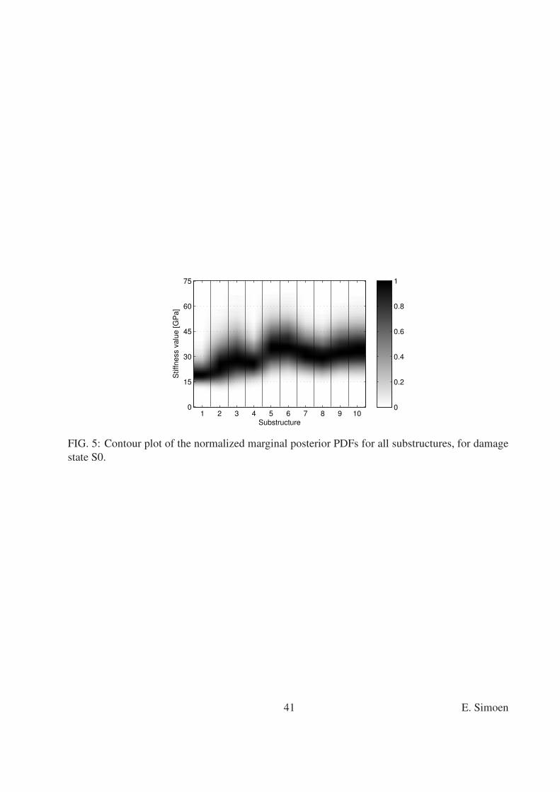
Results for damage state S0 The normalized marginal posterior PDFs for S0 are shown in Fig-416
ure 5; Table 3 reports the corresponding MAP estimate, and the mean value, standard deviation and417
coefficient of variation for each of the marginal PDFs. Also found in this table are the MAP values418
as obtained through minimization of the MAP objective function defined in Eq. (25); the uncon-419
strained optimization is performed in Matlab using a local gradient-based optimization algorithm420
through the standard Matlab routine fminunc.421
Comparing the MAP estimates θMAPopt and θMAP
MCMC as obtained through the deterministic opti-422
mization and the MCMC scheme, respectively, it is found that the values are very similar but not423
identical. Examination of the MAP residuals (i.e. J(S0)MAP, J
(S0)ML and J
(S0)MAPr evaluated at the MAP424
estimates) confirms that both MAP estimates are in fact very close, exhibiting residuals differing425
by less than 0.1%, although the MAP estimate obtained from the deterministic updating routine al-426
ways results in smaller residuals (J(S0)MAP,opt = −301.5 and J
(S0)MAP,MCMC = −301.2). This difference427
is most likely explained by the fact that the estimates are obtained through algorithms with very428
different objectives. The gradient-based optimization routine is specifically designed to find the429
MAP estimate, whereas the sampling method randomly searches the whole parameter space and is430
therefore sometimes less effective and less accurate in finding the global optimum.431
18 E. Simoen

Furthermore, it is found that the MAP objective function in this case exhibits non-smooth be-432
havior (most likely due to mode shape matching), which implies that the joint posterior PDF is433
most likely not peaked at a single point but rather exhibits many local maxima of similar prob-434
ability, making this a locally identifiable case (Katafygiotis and Beck 1998; Yuen 2010a). This435
situation is commonly encountered in Bayesian updating applications, and here further explains436
the difference between the two obtained MAP estimates. In the following, only the MCMC results437
are discussed in further detail.438
When examining the MAP-estimate and posterior mean values, it is clear that the effective439
stiffness in the undamaged state of the building was initially underestimated in most substructures,440
except for the bottom substructure 1, which shows a low value compared to the initial value θinit1 .441
Furthermore, among all the stiffness parameters, this bottom substructure stiffness is best identified442
from the data and prior information, as the COV is reduced from 35% to about 24%. For the top443
seven substructures, the uncertainty is reduced only to a very limited extent below the prior COV444
of 25%: the posterior COV-values range from 23% to 24.8%. In Figure 6, the normalized prior445
and posterior marginal PDFs are compared for substructures 1 and 5, which immediately confirms446
these findings: the posterior PDF for the bottom substructure has become much narrower, whereas447
for substructure 5 the posterior PDF is practically the same as the prior PDF. It should be noted448
here that it is apparent that both posterior PDFs are not Gaussian, which implies that mean values,449
standard deviations and associated COV values should be interpreted with appropriate care.450
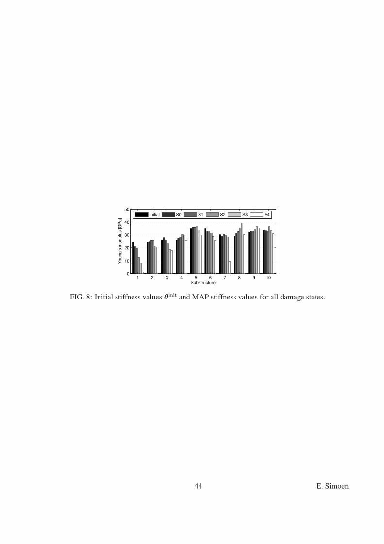
Results for damage states S1 to S4 In Figures 7a–7d, contour plots of the posterior marginal451
PDFs of the effective stiffness parameters θM are shown for damage states S1 to S4. The MAP-452
estimates (obtained through MCMC) of the stiffness values are compared in Figure 8 for all dam-453
age states, the corresponding values are reported in Table 4, together with the posterior marginal454
coefficients of variation.455
The MAP stiffness values generally reduce as the damage increases, especially the stiffness456
in the bottom substructures – where the actual damage from the shake table tests is concentrated.457
19 E. Simoen

The most drastic stiffness reduction occurs for substructure 1, where the MAP stiffness at S4458
decreases to about 1 GPa due to the very high level of damage. For some substructures, sometimes459
a small increase in MAP stiffness is found for a higher damage state, which is most likely caused460
by insensitivity of the model predictions to changes in these parameter values, resulting in the461
identifiability issues discussed above. This is corroborated by the fact that the posterior uncertainty462
regarding these substructures remains largely the same over all damage states.463
The significantly decreased stiffness value for substructure 7 in damage state S4 was also464
observed in the previously performed deterministic damage identification study (Moaveni et al.465
2010), where it was determined to be a false alarm. Most likely the low stiffness value is explained466
by the fact that the updating parameters will also account for damage in other structural elements467
that are not included in the updating scheme, such as the floor slabs or the flange wall. Note also468
the increased stiffness values in adjacent substructure 8, which most likely compensate for the469
stiffness decrease observed in substructure 7.470
Overall, the lower part of the structure (substructures 1–3) shows a larger COV reduction com-471
pared to the top substructures, especially in states S0 and S1, and particularly for the bottom472
substructure, where the posterior COV is even reduced to about half of the prior COV in S4. These473
observations are most likely explained by considering modal curvatures: firstly, the lower sec-474
tion of the structure is in any case subjected to higher modal curvatures, meaning the modal data475
are more sensitive to local stiffness changes and thus provide more information for the updating476
scheme in these areas. Moreover, structural damage results in an additional increase in modal cur-477
vature, explaining the substantial uncertainty reduction in the most damaged bottom substructure478
1. This also implies that, as the damage increases, the data become relatively less informative re-479
garding substructures with less extensive damage. Examining the posterior COV-values for higher480
damage levels S3 and S4 confirms this statement: for substructures 2–10 the uncertainty no longer481
reduces, and sometimes even increases slightly due to this effect.482
All these findings indicate that the available data are not always as informative regarding the483
chosen model parameters. This also implies that the available prior information plays an important484
20 E. Simoen

role in the results obtained through the Bayesian inference scheme. In order to confirm these state-485
ments and to obtain more insight into the underlying causes of these findings, a detailed resolution486
and uncertainty analysis may be carried out, as presented in the next section.487
RESOLUTION ANALYSIS488
The first step in a resolution analysis typically consists in determining quantities such as MAP489
estimates, posterior mean values and standard deviations, which yield basic insight into the resolu-490
tion of the parameters. However, standard deviations do not provide information regarding possible491
correlations between parameters, therefore the prior and posterior covariance matrices, denoted as492
Spr and Spo respectively, may be calculated to this end. Usually, the off-diagonal correlation val-493
ues are most easily interpreted and compared by computing the prior and posterior correlation494
coefficient matrices.495
To further investigate the resolution of (combinations of) the parameters, one could revert to496
Principal Component Analysis (PCA), where the correlated posterior variables are transformed to497
a set of mutually orthogonal (uncorrelated) variables by transforming the posterior data to a new498
orthogonal coordinate system. The coordinates of this new system are termed the principal com-499
ponents. The transformation is done in such a way that the first principal component corresponds500
to a direction in the parameter space that exhibits the largest variability in the posterior data; in501
other words, the principal components correspond to linear combinations of the original variables502
(or parameters) ranked according to decreasing posterior variance. The principal components cor-503
respond to the set of eigenvectors of the posterior covariance matrix Spo. The eigenvectors are504
ranked according to increasing associated eigenvalue, which corresponds to increasing posterior505
variance.506
Although PCA is an interesting technique to investigate the posterior resolution of the param-507
eters in the parameter space, it does not take into account any information contained in the prior508
information. This is why several authors (Tarantola 2005; Duijndam 1988) propose to examine509
21 E. Simoen

instead the solution of the following extended eigenvalue problem:510
SpoX = ΛSprX (27)511
It can be shown that the eigenvectors in X correspond to mutually orthogonal directions in the512
parameter space ranked according to decreasing reduction from prior to posterior variance, when513
ranked according to increasing eigenvalue. Each eigenvalue gives a measure for the ratio of pos-514
terior to prior variance in the corresponding direction in the parameter space, which means that515
the eigenvector associated with the smallest eigenvalue corresponds to a direction in the parameter516
space that shows the largest reduction from prior to posterior variance. In other words, the values517
of the eigenvalues express the relative degree of the reduction from prior to posterior variance in518
the principal directions in the parameter space.519
Relation to information entropy520
The information entropy is often used as a measure of the resulting uncertainty in the Bayesian521
estimates of the model parameters (Papadimitriou et al. 2000). For the posterior PDF, it is defined522
as:523
h(θ) = E [− log p(θ|d)] (28)524
Under certain asymptotic conditions (i.e. global identifiability (Katafygiotis and Beck 1998),525
or availability of a large amount of data compared to the prior information, such that the posterior526
PDF can be approximated by a Gaussian PDF around the ML or MAP point), the information527
entropy can be approximated as (Papadimitriou 2004):528
h(θ) ≈1
2N log(2πe)−
1
2log[
detQ(θML)]
(29)529
where Q denotes the Fisher Information Matrix (FIM), evaluated at the maximum likelihood point530
θML. The FIM is equal to the negative of the Hessian of the log likelihood, and it can be shown531
that this Hessian is (approximately) equal to the negative inverse of the posterior covariance matrix532
22 E. Simoen

(Papadimitriou et al. 1997). This in fact corresponds to assuming that the posterior PDF can533
be asymptotically approximated by a Gaussian PDF centered at the MAP or ML point, with a534
posterior covariance matrix Spo, as the entropy expression in Eq. (29) can be reformulated as:535
h(θ) ≈1
2log[
(2πe)N detSpo
]
(30)536
which can be recognized as the information entropy of a multivariate Gaussian PDF.537
The entropy discrepancy ∆h may be computed as a measure of the information that was gained538
from the observations. It is a non-negative scalar (as adding information always leads to decreasing539
entropy) which is defined as:540
∆h = hpr − hpo (31)541
Using the approximative entropy expression in Eq. (29), the following approximation for the542
entropy discrepancy is obtained:543
∆h ≈ −1
2log det
(
S−1pr Spo
)
= −1
2
Nθ∑
k=1
log λk (32)544
where λk are the eigenvalues of the eigenvalue problem defined in Eq. (27). This means that545
by computing the values dk = −12log λk corresponding to the eigenvectors (or directions in the546
parameter space) Xk, the relative contribution of the different directions to the total resolution can547
be quantified.548
Resolution analysis for the seven-story test structure549
The posterior correlation coefficient matrix for the substructure stiffnesses is shown in Figure550
9a for damage state S0, from which it can be deduced that, in contrast to the prior situation, the551
model parameters are a posteriori no longer independent variables. However, the correlations552
between the model parameters generally remain very limited, except for the bottom substructures553
where correlation coefficients of −0.42 are attained. Note that the occurring correlations are mostly554
negative, which is to be expected as contrasting stiffnesses (i.e. high in one and low in the other)555
23 E. Simoen

in (adjacent) substructures would explain the data almost equally well.556
In Figure 9b, the first and last two (normalized) eigenvectors or parameter combinations are557
shown, corresponding to the best and worst resolved directions in the parameter space. It is clear558
that the best resolved parameter combination contains predominantly the first substructure stiff-559
ness, whereas the two worst resolved directions contain all seven of the top substructure stiffness560
values. This is in very good agreement with the previously discussed results. By examining the561
eigenvalues associated with these eigenvectors, their relative contributions to the total resolution562
can be quantified in terms of entropy reduction. In this case, the total entropy reduction ∆h equals563
1.21, of which a part of (−1/2 log λ1 =) 0.92 or 76% is contributed by reduction in the direction564
X1. Directions X9 and X10 together contribute a mere 0.04% to the total entropy reduction, which565
also confirms the results found above. Note that, even though the conditions for using the approxi-566
mate entropy expressions may not be completely fulfilled for this particular case study, the entropy567
analysis yields important insights into the resolution of the different parameter combinations.568
For damage states S1 to S3, very similar results are found. In Figure 10a, the posterior cor-569
relation coefficient matrix is shown for damage state S4, and in Figure 10b, the best and two570
worst resolved directions in the parameter space are displayed. The negative correlations between571
adjacent substructures 6–9 , and especially between substructures 7 and 8 (ρ7,8 = −0.46) are im-572
mediately apparent; substructure 7 even shows a negative correlation with all other substructures.573
This corresponds to the observations made above regarding the false alarm and compensation by574
substructure 8.575
The eigenvector analysis confirms that the effective stiffness of substructure 1 is by far the best576
resolved feature, accounting for almost 80% of the entropy reduction through the data in dam-577
age state S4. Furthermore, the worst resolved parameter directions encompass almost all other578
substructures, especially substructures 6–8, indicating that very little information about these pa-579
rameters can be obtained from the data used in this study. Therefore, large uncertainty remains580
associated with the false alarm detected in the previous analyses.581
It is confirmed that the worst resolved features incorporate the top substructures 4–10 for all582
24 E. Simoen

damage states, which indicates that the FE model of the seven-story test building is most likely583
over-parameterized, as the data appears to contain very little to no information regarding these top584
seven parameters.585
CONCLUSIONS586
In this paper, Bayesian linear FE model updating is used for uncertainty quantification in the587
assessment of progressive damage in a seven-story reinforced concrete building slice subjected to588
seismic tests on the USCSD-NEES shake table. To this end, experimentally identified modal data589
obtained in five different damage states are employed. In the Bayesian FE model updating ap-590
proach, a zero-mean uncorrelated Gaussian prediction error is assumed, and to construct the prior591
PDFs, the Maximum A Posteriori (MAP) estimate of a certain damage state is adopted as the Max-592
imum A Priori estimate of the next damage state. The posterior joint PDF of the substructure stiff-593
ness parameters is estimated using a MCMC approach and the MAP results are validated through594
a deterministic updating scheme based on the Bayesian approach. The results of the Bayesian FE595
model updating scheme are assessed further by performing a detailed resolution analysis, which596
allows for improved insight into which (and to what extent) characteristics of the damaged struc-597
ture are resolved through the Bayesian scheme using the identified modal data. Furthermore, it is598
shown how the incorporation of prior information relates to the regularization of the corresponding599
deterministic FE model updating problem.600
Overall, the Bayesian approach succeeded in identifying the damage in the seven-story struc-601
ture and in quantifying the corresponding uncertainties at all damage states. It was found that602
the data contain little information concerning the top stories of the building, as the uncertainty603
on the stiffness parameters representing this area could not be reduced through the observed data.604
This was confirmed by a detailed resolution analysis, which showed that parameter combinations605
containing the upper seven substructures were always least resolved by the available data. How-606
ever, the lower substructures, and the bottom substructure 1 in particular, are well resolved by the607
data, most likely due to the higher damage level and higher modal curvatures in these areas of the608
structure.609
25 E. Simoen

These findings lead to the conclusion that for this structure, damage can be detected (SHM610
Level 1 (Rytter 1993)) effectively, but that for the purpose of reducing the uncertainty regarding611
damage quantification and localization (SHM levels 2–3) in the upper stories, more elaborate ex-612
perimental data are desirable. This can be accomplished by increasing the number of mode shapes613
and/or measurement DOFs, or by including other types of modal data such as modal strains.614
REFERENCES615
Beck, J. and Au, S.-K. (2002). “Bayesian updating of structural models and reliability using616
Markov Chain Monte Carlo simulation.” ASCE Journal of Engineering Mechanics, 128(4), 380–617
391.618
Beck, J. and Katafygiotis, L. (1998). “Updating models and their uncertainties. I: Bayesian statis-619
tical framework.” ASCE Journal of Engineering Mechanics, 124(4), 455–461.620
Beck, J. and Yuen, K.-V. (2004). “Model selection using response measurements: Bayesian prob-621
abilistic approach.” ASCE Journal of Engineering Mechanics, 130(2), 192–203.622
Box, G. and Tiao, G. (1973). Bayesian inference in statistical analysis. Addison-Wesley.623
Ching, J. and Chen, Y.-C. (2007). “Transitional Markov Chain Monte Carlo method for Bayesian624
model updating, model class selection, and model averaging.” ASCE Journal of Engineering625
Mechanics, 133(7), 816–832.626
Cox, R. (1946). “Probability, frequency and reasonable expectation.” American Journal of Physics,627
14(1), 1–13.628
Duijndam, A. (1988). “Bayesian estimation in seismic inversion. Part II: Uncertainty analysis.”629
Geophysical Prospecting, 36(8), 899–918.630
Filippou, F. and Constantinides, M. (2004). “Fedeaslab getting started guide and simulation exam-631
ples.” Technical report NEESgrid-2004-22, <http://fedeaslab.berkeley.edu>.632
Friswell, M. and Mottershead, J. (1995). Finite element model updating in structural dynamics.633
Kluwer Academic Publishers, Dordrecht, The Netherlands.634
Gamerman, D. (1997). Markov Chain Monte Carlo: stochastic simulation for Bayesian inference.635
Chapman & Hall, London.636
26 E. Simoen

Haario, H., Laine, M., Mira, A., and Saksman, E. (2006). “DRAM: Efficient adaptive MCMC.”637
Statistics and Computing, 16(4), 339–354.638
Haario, H., Saksman, E., and Tamminen, J. (2001). “An adaptive Metropolis algorithm.”639
Bernouilli, 7(2), 223–242.640
Heylen, W., Lammens, S., and Sas, P. (1997). Modal analysis theory and testing. Department of641
Mechanical Engineering, Katholieke Universiteit Leuven, Leuven, Belgium.642
Jaynes, E. (1957). “Information theory and statistical mechanics.” The Physical Review, 106(4),643
620–630.644
Jaynes, E. (2003). Probability Theory. The Logic of Science. Cambridge University Press, Cam-645
bridge, UK.646
Katafygiotis, L. and Beck, J. (1998). “Updating models and their uncertainties. II: Model identifi-647
ability.” ASCE Journal of Engineering Mechanics, 124(4), 463–467.648
Mehta, M. (2004). Random Matrices. Elsevier, San Diego, CA, 3rd edition.649
Moaveni, B., Barbosa, A., Conte, J., and Hemez, F. (2007). “Uncertainty analysis of modal param-650
eters obtained from three system identification methods.” Proceedings of IMAC-XXV, Interna-651
tional Conference on Modal Analysis, Orlando, Florida, USA (February).652
Moaveni, B., Conte, J., and Hemez, F. (2009). “Uncertainty and sensitivity analysis of damage653
identification results obtained using finite element model updating.” Computer-Aided Civil and654
Infrastructure Engineering, 24(5), 320–334.655
Moaveni, B., He, X., Conte, J., and Restrepo, J. (2010). “Damage identification study of a seven-656
story full-scale building slice tested on the UCSD-NEES shake table.” Structural Safety, 32,657
347–356.658
Moaveni, B., He, X., Conte, J., Restrepo, J., and Panagiotou, M. (2011). “System identification659
study of a 7-story full-scale building slice tested on the USCD-NEES shake table.” ASCE Jour-660
nal of Engineering Mechanics, 137(6), 705–717.661
Moaveni, B., Barbosa, A.R., Conte, J.P. and Hemez, F. (2012). “Uncertainty analysis of system662
identification results obtained for a seven story building slice tested on the UCSD-NEES shake663
27 E. Simoen

table.” Structural Control and Health Monitoring, under review.664
Mosegaard, K. and Tarantola, A. (1995). “Monte Carlo sampling of solutions to inverse problems.”665
Journal of Geophysical Research, 100, 12431–12447.666
Mottershead, J. and Friswell, M. (1993). “Model updating in structural dynamics: a survey.” Jour-667
nal of Sound and Vibration, 167(2), 347–375.668
Muto, M. and Beck, J. (2008). “Bayesian updating and model class selection for hysteretic struc-669
tural models using stochastic simulation.” Journal of Vibration and Control, 14(1–2), 7–34.670
Panagiotou, M., Restrepo, J., and Conte, J. (2011). “Shake table test of a full-scale 7-story building671
slice. Phase I: rectangular wall.” ASCE Journal of Structural Engineering, 137(6), 691–704.672
Papadimitriou, C. (2004). “Optimal sensor placement for parametric identification of structural673
systems.” Journal of Sound and Vibration, 278, 923–947.674
Papadimitriou, C., Beck, J., and Au, S. (2000). “Entropy-based optimal sensor location for struc-675
tural model updating.” Journal of Vibration and Control, 6(5), 781–800.676
Papadimitriou, C., Beck, J., and Katafygiotis, L. (1997). “Asymptotic expansions for reliability and677
moments of uncertain systems.” ASCE Journal of Engineering Mechanics, 123(12), 1219–1229.678
Peeters, B. and De Roeck, G. (2001). “Stochastic system identification for operational modal anal-679
ysis: A review.” ASME Journal of Dynamic Systems, Measurement, and Control, 123(4), 659–680
667.681
Reynders, E. and De Roeck, G. (2008). “Reference-based combined deterministic-stochastic sub-682
space identification for experimental and operational modal analysis.” Mechanical Systems and683
Signal Processing, 22(3), 617–637.684
Reynders, E., Pintelon, R., and De Roeck, G. (2008). “Uncertainty bounds on modal parameters685
obtained from Stochastic Subspace Identification.” Mechanical Systems and Signal Processing,686
22(4), 948–969.687
Rytter, A. (1993). “Vibration based inspection of civil engineering structures.” Ph.D. thesis, Aal-688
borg University, Aalborg University.689
Schevenels, M., Lombaert, G., Degrande, G., and Francois, S. (2008). “A probabilistic assessment690
28 E. Simoen

of resolution in the SASW test and its impact on the prediction of ground vibrations.” Geophys-691
ical Journal International, 172(1), 262–275.692
Sibilio, E., Ciampoli, M., and Beck, J. (2007). “Structural health monitoring by Bayesian upating.”693
Proceedings of the ECCOMAS Thematic Conference on Computational Methods in Structural694
Dynamics and Earthquake Engineering, Rethymno, Crete, Greece (June).695
Sohn, H. and Law, K. (1997). “A Bayesian probabilistic approach for structure damage detection.”696
Earthquake Engineering and Structural Dynamics, 26(12), 1259–1281.697
Soize, C. (2000). “A nonparametric model of random uncertainties for reduced matrix models in698
structural dynamics.” Probabilistic Engineering Mechanics, 15, 277–294.699
Soize, C. (2003). “Probabilites et modelisation des incertitudes: elements de base et concepts700
fondamentaux (May).701
Soize, C. (2008). “Construction of probability distributions in high dimensions using the maximum702
entropy principle: applications to stochastic processes, random fields and random matrices.”703
International Journal for Numerical Methods in Engineering, 75, 1583–1611.704
Soize, C. (2010). “Generalized probabilistic approach of uncertainties in computational dynam-705
ics using random matrices and polynomial chaos decompositions.” International Journal for706
Numerical Methods in Engineering, 81(8), 939–970.707
Soize, C. (2011). “Stochastic modeling of uncertainties in computational structural dynamics –708
recent theoretical advances.” Journal of Sound and Vibration doi:10.1016/j.jsv.2011.10.010.709
Tarantola, A. (2005). Inverse problem theory and methods for model parameter estimation. SIAM,710
Philadelphia, USA.711
Teughels, A., Maeck, J., and De Roeck, G. (2002). “Damage assessment by FE model updating712
using damage functions.” Computers and Structures, 80(25), 1869–1879.713
Vanik, M., Beck, J., and Au, S. (2000). “Bayesian probabilistic approach to structural health mon-714
itoring.” ASCE Journal of Engineering Mechanics, 126(7), 738–745.715
Yuen, K.-V. (2010a). Bayesian methods for structural dynamics and civil engineering. John Wiley716
& Sons, Singapore, 1st edition.717
29 E. Simoen

Yuen, K.-V. (2010b). “Recent developments of Bayesian model class selection and applications in718
civil engineering.” Structural Safety, 32(5), 338–346.719
Yuen, K.-V. and Katafygiotis, L. (2002). “Bayesian modal updating using complete input and720
incomplete response noisy measurements.” ASCE Journal of Engineering Mechanics, 128(3),721
340–350.722
Yuen, K.-V., Katafygiotis, L., Papadimitriou, C., and Mickleborough, N. (2001). “Optimal sen-723
sor placement methodology for identification with unmeasured excitation.” ASME Journal of724
Dynamic Systems, Measurement, and Control, 123(4), 677–686.725
30 E. Simoen

List of Tables726
1 The five damage states and corresponding imposed historical earthquake records. . 32727
2 Experimentally identified natural frequencies and damping ratios for the five dam-728
age states. . . . . . . . . . . . . . . . . . . . . . . . . . . . . . . . . . . . . . . . 33729
3 Initial values, MAP estimates obtained through deterministic updating and MCMC,730
posterior mean values µ, standard deviations σ and coefficients of variation (COV)731
for S0. . . . . . . . . . . . . . . . . . . . . . . . . . . . . . . . . . . . . . . . . . 34732
4 MAP-values and coefficients of variation (COV) for the 10 substructure stiffnesses,733
for all damage states. . . . . . . . . . . . . . . . . . . . . . . . . . . . . . . . . . 35734
31 E. Simoen

TABLE 1: The five damage states and corresponding imposed historical earthquake records.
Damage Earthquake record
state Earthquake Component Recorded at M
S0 None - - -
S1 1971 San Fernando longitudinal Van Nuys 6.6
S2 1971 San Fernando transversal Van Nuys 6.6
S3 1994 Northridge longitudinal Oxnard Blvd. 6.7
S4 1994 Northridge 360 degree Oxnard Blvd. 6.7
32 E. Simoen

TABLE 2: Experimentally identified natural frequencies and damping ratios for the five damage
states.
Damage fexp [Hz] ξexp [%]
state Mode 1 Mode 2 Mode 3 Mode 1 Mode 2 Mode 3
S0 1.91 10.51 24.51 2.3 2.4 0.5
S1 1.88 10.21 24.31 2.9 2.7 0.6
S2 1.67 10.16 22.60 1.3 1.4 0.9
S3 1.44 9.23 21.82 2.7 1.3 1.4
S4 1.02 5.67 15.10 1.0 1.7 1.0
33 E. Simoen

TABLE 3: Initial values, MAP estimates obtained through deterministic updating and MCMC,
posterior mean values µ, standard deviations σ and coefficients of variation (COV) for S0.
Sub- S0 [GPa]
structure θinit θMAPopt θMAP
MCMC µ(σ) COV [%]
1 24.50 19.71 20.91 21.33 (5.10) 23.9
2 24.50 25.05 24.83 27.41 (8.77) 32.0
3 26.00 28.74 27.87 31.56 (9.86) 31.3
4 26.00 26.52 27.79 28.07 (6.75) 24.0
5 34.80 35.07 36.06 37.23 (9.25) 24.8
6 34.80 36.18 32.56 38.12 (9.19) 24.1
7 30.20 31.96 29.14 33.43 (7.69) 23.0
8 28.90 28.73 31.53 31.42 (7.26) 23.1
9 32.10 31.81 32.67 35.14 (8.33) 23.7
10 33.50 33.61 33.12 36.05 (8.93) 24.8
34 E. Simoen

TABLE 4: MAP-values and coefficients of variation (COV) for the 10 substructure stiffnesses, for
all damage states.
Sub- S0 S1 S2 S3 S4
structure MAP COV MAP COV MAP COV MAP COV MAP COV
[GPa] [%] [GPa] [%] [GPa] [%] [GPa] [%] [GPa] [%]
1 20.91 23.9 19.56 23.1 12.66 24.4 7.96 22.7 1.16 19.1
2 24.83 32.0 25.92 33.0 25.92 38.3 21.61 40.1 20.53 37.7
3 27.87 31.3 26.17 31.7 23.97 35.6 18.43 40.8 17.80 40.9
4 27.79 24.1 28.36 24.3 30.12 25.0 30.04 25.9 25.81 27.0
5 36.06 24.8 36.06 24.7 37.03 25.4 33.70 25.3 29.94 27.6
6 32.56 24.1 32.36 24.3 31.27 24.6 28.80 24.9 25.82 29.0
7 29.14 23.0 30.35 23.2 29.40 23.4 28.43 24.6 9.68 36.2
8 31.53 23.1 32.68 23.2 35.44 22.5 39.10 24.0 30.18 32.7
9 32.67 23.7 33.06 22.9 33.94 22.7 36.49 24.5 35.07 27.3
10 33.12 24.8 33.01 24.0 36.53 24.3 33.13 25.4 31.18 25.8
35 E. Simoen

List of Figures735
1 (a) Seven-story test structure and (b) elevation view. . . . . . . . . . . . . . . . . . 37736
2 First three longitudinal mode shapes obtained at damage state S0. . . . . . . . . . 38737
3 (a) FE model of the seven-story test structure and (b) definition of the substructures738
along the main wall. . . . . . . . . . . . . . . . . . . . . . . . . . . . . . . . . . . 39739
4 (a) Contour plot of the normalized marginal prior PDFs and (b) marginal prior PDF740
for substructure 1, for damage state S0. . . . . . . . . . . . . . . . . . . . . . . . 40741
5 Contour plot of the normalized marginal posterior PDFs for all substructures, for742
damage state S0. . . . . . . . . . . . . . . . . . . . . . . . . . . . . . . . . . . . 41743
6 Normalized marginal prior PDF (dashed line) and posterior PDF (solid line) for (a)744
substructure 1 and (b) substructure 5, for damage state S0. . . . . . . . . . . . . . 42745
7 Contour plot of the normalized marginal posterior PDFs for all substructures, for746
damage states S1 to S4. . . . . . . . . . . . . . . . . . . . . . . . . . . . . . . . . 43747
8 Initial stiffness values θinit and MAP stiffness values for all damage states. . . . . . 44748
9 (a) Visualization of posterior correlation coefficient matrix where the relative size749
of the symbols represents the value of the negative (◦) and positive (�) correlation750
coefficients, and (b) the best (X1) and two worst (X9 and X10) resolved parameter751
combinations, for damage state S0. . . . . . . . . . . . . . . . . . . . . . . . . . . 45752
10 (a) Visualization of posterior correlation coefficient matrix where the relative size753
of the symbols represents the value of the negative (◦) and positive (�) correlation754
coefficients and (b) the best (X1) and two worst (X9 and X10) resolved parameter755
combinations, for damage state S4. . . . . . . . . . . . . . . . . . . . . . . . . . . 46756
36 E. Simoen

(a) (b)
FIG. 1: (a) Seven-story test structure and (b) elevation view.
37 E. Simoen

FIG. 2: First three longitudinal mode shapes obtained at damage state S0.
38 E. Simoen
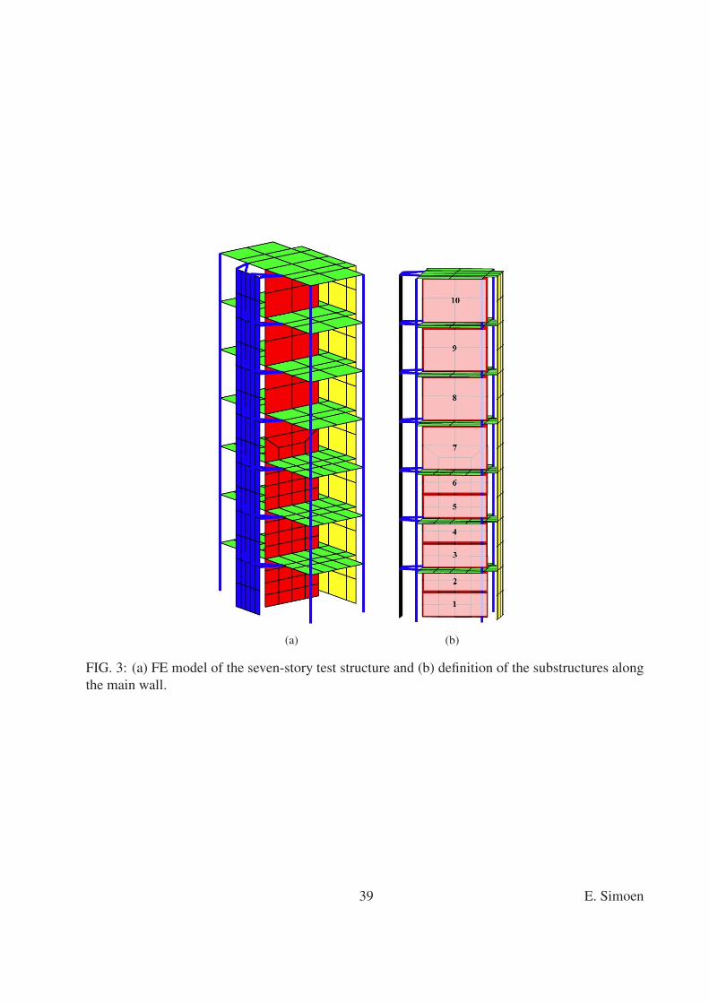
(a) (b)
FIG. 3: (a) FE model of the seven-story test structure and (b) definition of the substructures along
the main wall.
39 E. Simoen

Substructure
Stiffness v
alu
e [G
Pa]
1 2 3 4 5 6 7 8 9 10
75
60
45
30
15
0 0
0.2
0.4
0.6
0.8
1
(a)
0 20 40 600
0.01
0.02
0.03
0.04
0.05
Substructure stiffness θ1 [GPa]
PD
F [1/G
Pa]
(b)
FIG. 4: (a) Contour plot of the normalized marginal prior PDFs and (b) marginal prior PDF for
substructure 1, for damage state S0.
40 E. Simoen
Substructure
Stiffness v
alu
e [G
Pa]
1 2 3 4 5 6 7 8 9 10
75
60
45
30
15
0 0
0.2
0.4
0.6
0.8
1
FIG. 5: Contour plot of the normalized marginal posterior PDFs for all substructures, for damage
state S0.
41 E. Simoen

0 20 40 600
0.2
0.4
0.6
0.8
1
Substructure stiffness θ1 [GPa]
PD
F [1/G
Pa]
(a)
0 20 40 600
0.2
0.4
0.6
0.8
1
Substructure stiffness θ5 [GPa]
PD
F [1/G
Pa]
(b)
FIG. 6: Normalized marginal prior PDF (dashed line) and posterior PDF (solid line) for (a) sub-
structure 1 and (b) substructure 5, for damage state S0.
42 E. Simoen

Substructure
Stiff
ness v
alu
e [
GP
a]
1 2 3 4 5 6 7 8 9 10
75
60
45
30
15
0 0
0.2
0.4
0.6
0.8
1
(a) S1
Substructure
Stiff
ness v
alu
e [
GP
a]
1 2 3 4 5 6 7 8 9 10
75
60
45
30
15
0 0
0.2
0.4
0.6
0.8
1
(b) S2
Substructure
Stiffness v
alu
e [G
Pa]
1 2 3 4 5 6 7 8 9 10
75
60
45
30
15
0 0
0.2
0.4
0.6
0.8
1
(c) S3
Substructure
Stiffness v
alu
e [G
Pa]
1 2 3 4 5 6 7 8 9 10
75
60
45
30
15
0 0
0.2
0.4
0.6
0.8
1
(d) S4
FIG. 7: Contour plot of the normalized marginal posterior PDFs for all substructures, for damage
states S1 to S4.
43 E. Simoen
1 2 3 4 5 6 7 8 9 100
10
20
30
40
50
Substructure
Yo
un
g‘s
mo
du
lus [
GP
a]
Initial S0 S1 S2 S3 S4
FIG. 8: Initial stiffness values θinit and MAP stiffness values for all damage states.
44 E. Simoen

1 2 3 4 5 6 7 8 9 10
1
2
3
4
5
6
7
8
9
10
Substructure
Substr
uctu
re
(a)
1 2 3 4 5 6 7 8 9 10
−1
−0.5
0
0.5
1
Substructure stiffness parameter θM
X1
X9
X10
(b)
FIG. 9: (a) Visualization of posterior correlation coefficient matrix where the relative size of the
symbols represents the value of the negative (◦) and positive (�) correlation coefficients, and (b)
the best (X1) and two worst (X9 and X10) resolved parameter combinations, for damage state S0.
45 E. Simoen

1 2 3 4 5 6 7 8 9 10
1
2
3
4
5
6
7
8
9
10
Substructure
Substr
uctu
re
(a)
1 2 3 4 5 6 7 8 9 10
−1
−0.5
0
0.5
1
Substructure stiffness parameter θM
X1
X9
X10
(b)
FIG. 10: (a) Visualization of posterior correlation coefficient matrix where the relative size of the
symbols represents the value of the negative (◦) and positive (�) correlation coefficients and (b)
the best (X1) and two worst (X9 and X10) resolved parameter combinations, for damage state S4.
46 E. Simoen