unclassified - defense technical information center · unclassified ad20 9 336 repdwed armed ......
TRANSCRIPT
UNCLASSIFIED
AD920 336
Repdwed
ARMED SERVICES TECHNICAL INFORMATION AGENCYARLINGTON HALL STATIONARLINGTON 12, VIRGINIA
UNCLASSIFIED
NOTICE: When government or other drawings, speci-fications or other data are used for any purposeother than in connection with a definitely relatedgovernment procurement operation, the U. S.Government thereby incurs no responsibility, nor anyobligation whatsoever; and the fact that the Govern-ment may have formulated, furnished, or in any waysupplied the said drawings, specifications, or otherdata is not to be regarded by implication or other-wise as in any manner licensing the holder or anyother person or corporation, or conveying any rightsor permission to manufacture, use or sell anypatented invention that may in any way be relatedthereto.
ASo-TDR,2-561 290 '336
DIFFUSION IN TITANIUM AND TITANIUM ALLOYS
TECHNICAL DOCUMENTARY REPORT NO. ASD-TDR-62-561
October 1962
Directorate of Materials and Processes
C,.• -.- • Aeronautical Systems Division
Air Force Systems Command
Wright-Patterson Air Force Base, Ohio
>.• YEARS
POF Project No. 7351, Task No. 735105S• £ MATERIALS ''
= I [ PROGRESS
(Prepared under Contract No. AF 33(616)-7656by the Armour Research Foundation, Chicago, Illinois;
Rodney P. Elliott, author.)
FMOEWRD
This report was prepared by Armour Research Foundation of Illinois Insti-tute of Technology under USAF Contract No. AF 33(616)-7656. This contract wasinitiated under Project No. 7351, "Metallc Materials," Task No. 735105, "HighStrength Metallic Materials." The work was administered under the direction ofthe Directorate of Materials and Processes, Deputy for Technology, AeronauticalSystem Division, with Mr. Paul L. Hendricks acting as project engineer.
This report covers work conducted during the period 1 November 1960 to28 February 1962.
The experimental work was carried out under the direction of Rodney P.Elliott, project engineer. Edward A. K-Ywe was project experimentalist. Perti-nent data are recorded in ARF Logbooks C 10731, C 11174, and C 11910. The re-search is identified at Armour Research Foundation as Project No. B 208, withthis final technical report designated ARF 2208-16.
ABSTRACT
The self-diffusion of titanium and the interdiffusion of aluminum,zirconium, molybdenum, vanadium, and oxygen in titanium have beeninvestigated in the temperature range 600"-1300"C. Diffusion couples wereprepared by roll-bonding or press-bonding techniques. Electron micro-probe methods were used to determine the penetration of the substitutionallydissolved solutes; vacuum fusion analysis was used to determine the penetra-tion of interstitially dissolved oxygen.
The determined diffusion may be summarized:
in DT = (-27. 14 ± 1.56) - (11,800 ± 3, 000)/RT for Zr in a-TiIn DT = (-4. 01 ± 1. 22) - (40, 100 ± 3, 300)/RT for Zr in 1-Ti
In DT = (-17. 19) - (28, 400)/RT for Mo in a-TiIn DT = (-9. 00 ± 0. 92) - (33, 100 ± 2, 400)/RT for Mo in 1-Ti
In DT = (-31. 39) - (3, 100)/RT for V in a-TiIn DT = (-4. 38 ± 1. 04) - (41, 400 ± 2, 800)/RT for V in 3-Ti
In DT = (-14. 94 1. 15) - (16,200* 2, Z00)/RT for 0 in a-Tiin DT = (+8. 37 * 2. 21) - (66, 800 7, 000)/RT for 0 in P-Ti
The electron microprobe analysis could not be used to determine thepenetration curves of aluminum in titanium because of the very high absorp-tion of characteristic aluminum X-radiation by titanium.
Tie self-diffusion of titanium was investigated by studying penetra-tion of Ti4, formed by bombtiding scandium with protons. Diffusion coupleswere formed by dissolving Ti -enriched TiO2 into the titanium. Self-diffusion of titanium may be summarized:
In DT = (-21. 08) - (5, 700)/RT for a-TiIn DT = (-8. 40) - (28, 600)/RT for 1-Ti
The diffusion equations for molybdenum and vanadium in a-titanium,and for the self-diffusion of titanium must be considered preliminary.
This report has been reviewed and is approved.
I. PERLMUTTERChief, Physical Metallurgy BranchMetals and Ceramics "LaboratoryDirectorate of Materials and Processes
i41
TABLE OF CONTENTS
Page
L INTRODUCTION ............... .................... 1
II. LITERATURE SURVEY ............. ................. 1
IIL DIFFUSION ANALYSIS METHODS .......... ............ 3
A. Interdiffusion .............. ..................... 3B. Self-Diffusion.. .................. 5
IV. EXPERIMENTAL PROGRAM .......... .............. 6
A. Selection of Alloys for InterdiffusionOf Al, Zr, Mo, V, and O in Titanium ....... ........ 6
B. Selection of Geometry for Study ofSelf-diffusion of Titanium ............... .......... 7
C. Production and Analysis of Diffusion Couples ....... ..... 8
1. Preparation of Alloys . . . .......... .......... 82. Preparation of Interdiffusion Couples .... ........ 83. Preparation of Self-diffusion Couples ......... .. 104. Diffusion Annealing ....... ............... .. 115. Penetration Curve Analysis for Substitutional
Solutes '.'.*...'.*.*.*.... .......... 126. Penetration Curve Analysis for Oxygen Diffusion. 147. Penetration Curves for Self-diffusion ......... ... 15
V. DISCUSSION ............... ..................... .. 16
REFERENCES ............. ..................... .. 20
APPENDIX I - THE PRODUCTION OF RADIOACTIVE Ti 4 4 . 54APPENDIX If- SAMPLE CALCULATIONS OF DIFFUSION
COEFFICIENTS ........ ............. .. 55
iv
LIST OF FIGURES
Figure Page
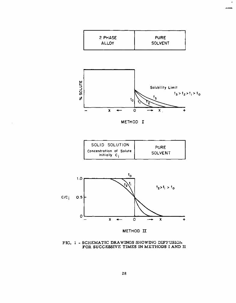
1 Schematic Drawings Showing Diffusion forSuccessive Times in Methods I and II . ........ 28
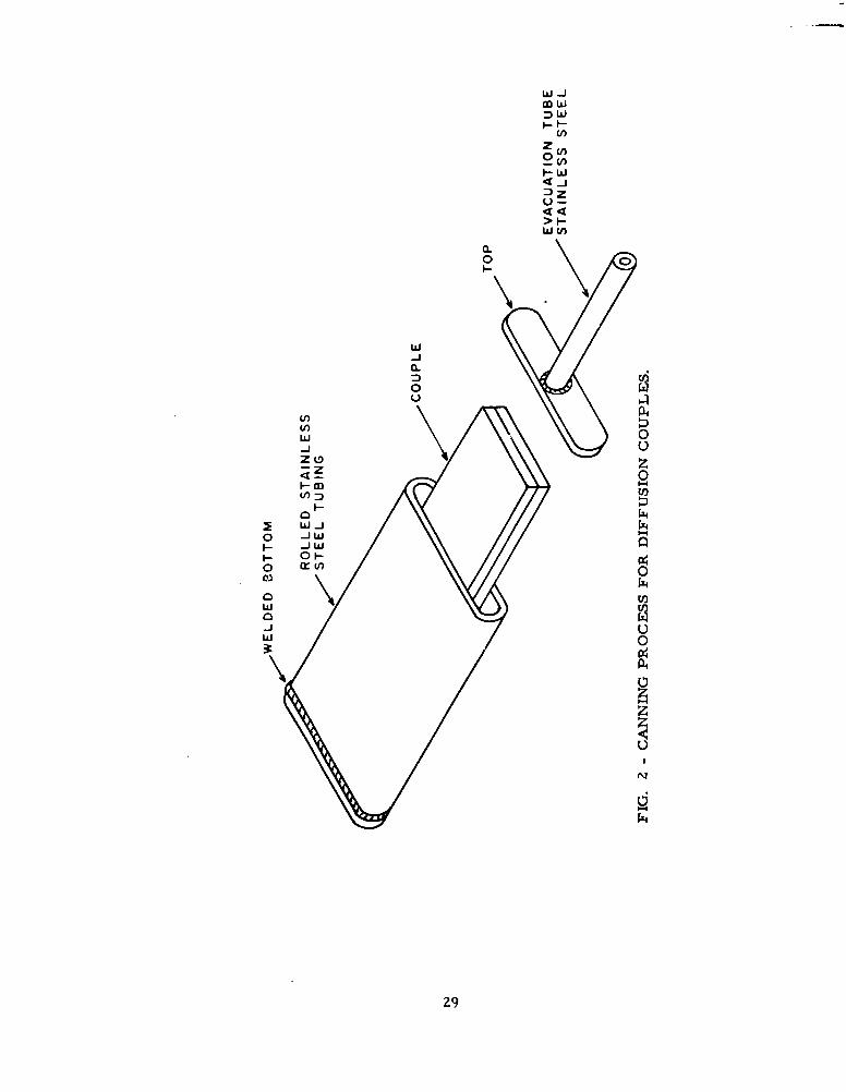
2 Canning Process for Diffusion Couples .......... ... 29
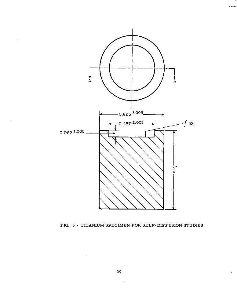
3 Titanium Specimen for Self-Diffusion Studies ..... .. 30
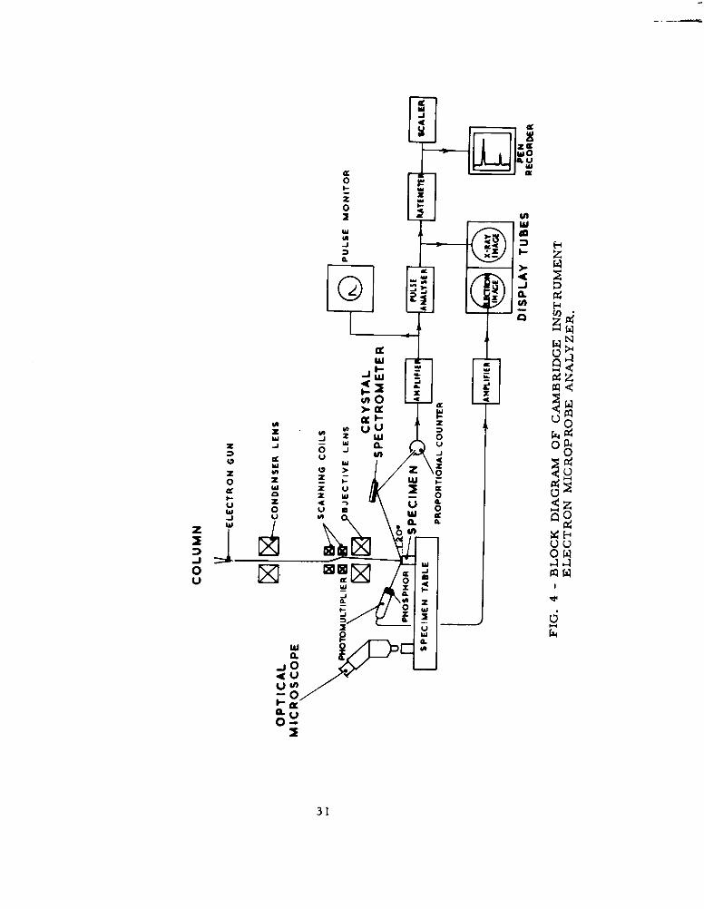
4 Block Diagram of Cambridge InstrumentElectron Microprobe Analyzer .......... .5..... .1
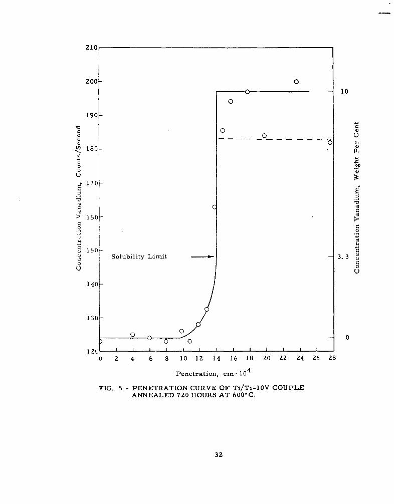
5 Penetration Curve of Ti/Ti-10V CoupleAnnealed 720 Hours at 6000C ..... ........... 32
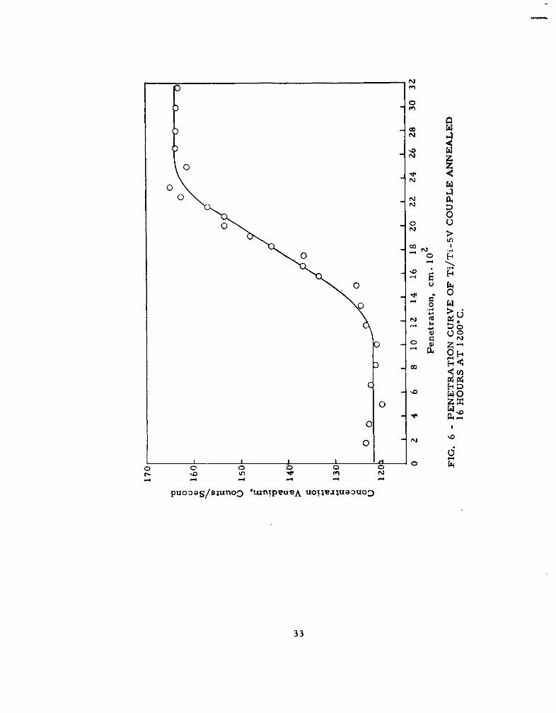
6 Penetration Curve of Ti/Ti-5V CoupleAnnealed 16 Hours at 12000C ......... ........... 33
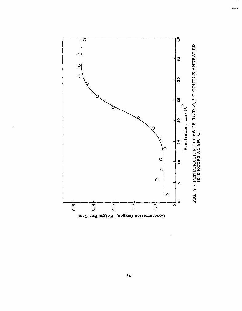
7 Penetration Curve of Ti/Ti-0. 5 0 CoupleAnnealed 1000 Hours at 8000C .C ..........
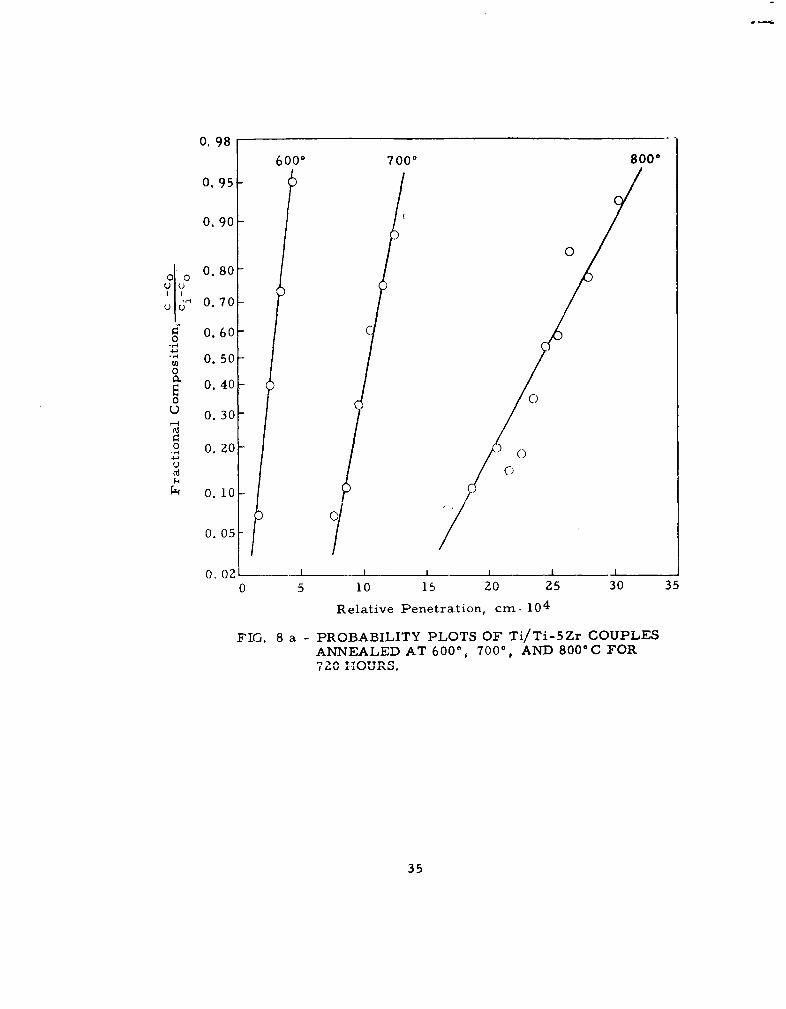
8a Probability Plots of Ti/Ti-5Zr CouplesAnnealed at 600%, 700%, and 800*C for 720 Hours . . 35
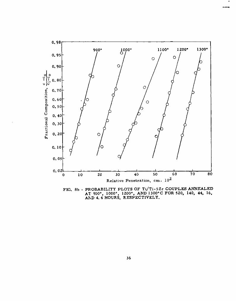
8b Probability Plots of Ti/Ti-5Zr CouplesAnnealed at 900, 1000%, 1200%, and 13000CFor 520, 140, 44, 16, and 4. 4 Hours, Respectively . 36
9a Probability Plots of Ti/Ti-7Mo CouplesAnnealed at 6000 and 8000 C for 720 Hours ........ 37
9b Probability Plots of Ti/Ti-SMo CouplesAnnealed at 900%, 1l00, and 12000 CFor 420, 92, and 48 Hours, Respectively. ......... 38
1Oa Probability Plots of Ti/Ti-10V CouplesAnnealed at 600* and 7000C for 720 Hours....... 39
10b Probability Plots of Ti/Ti-5V CouplesAnnealed at 900%, 1000, 1100%, 1200, and 1300C 40For 520, 140, 44, 16, and 4. 4 Hours, Respectively . .
l la Probability Plots of Ti/Ti-0. 5 0 CouplesAnnealed at 600%, 700%, and 800*C for 1000 Hours. . 41
1lb Probability Plots of Ti/Ti-O. 50 CouplesAnnealed at 900", 1000, 1l00 1200" and 13000CFor 900, 135, 48, 14, and 4. 8 hours, Respectively . 42
V
LIST OF FIGURES(Continued)
Figure Page
12 Summary of Diffusion Coefficients for Zirconium,Molybdenum, Vanadium, and Oxygen in a-Titanium 43
13 Summary of Diffusion Coefficients for Zirconium,Molybdenum, Vanadium, and Oxygen in P-Titanium .
14 Decay Scheme of Ti 4 4 . . .. .. .. .. .. .. .. .. .. .. .. .. 45
15a Penetration Curve of Self-Diffusion Couple 46Annealed at 6000C for 60 Days ......... .
15b Penetration Curve of Self-Diffusion Couple 47Annealed at 700°C for 60 Days ..........
15c Penetration Curve of Self-Diffusion Couple 48Annealed at 8000C for 60 Days ..........
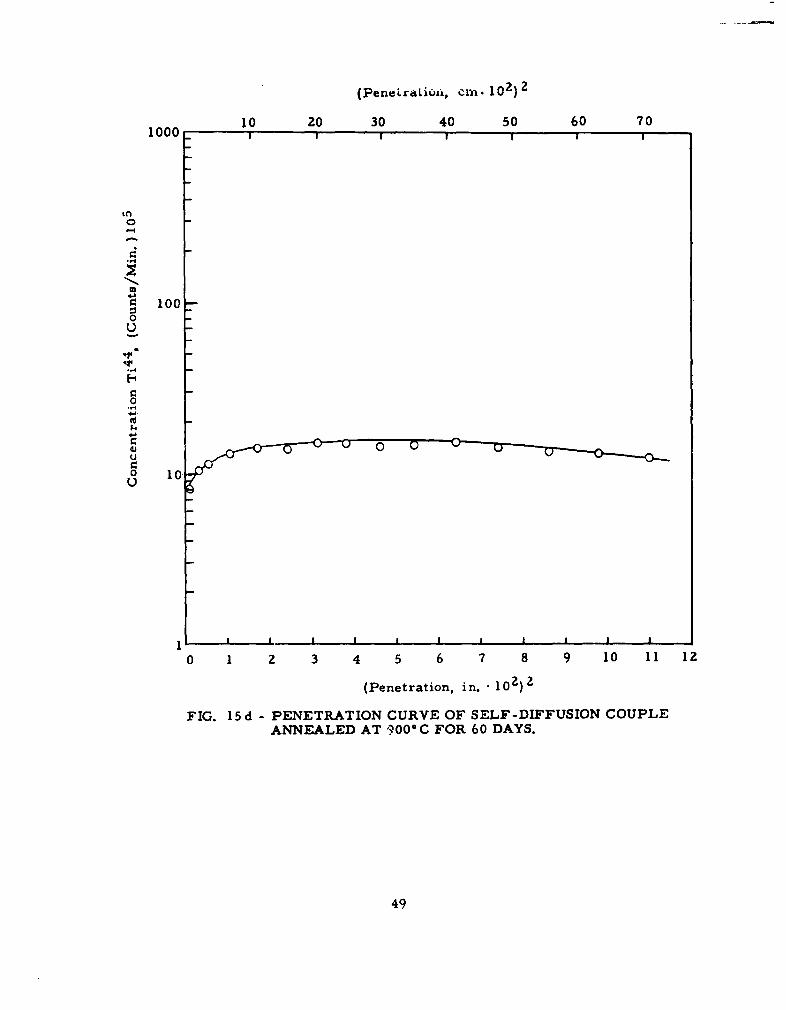
15d Penetration Curve of Self-Diffusion Couple 49Annealed at 9000C for 60 Days
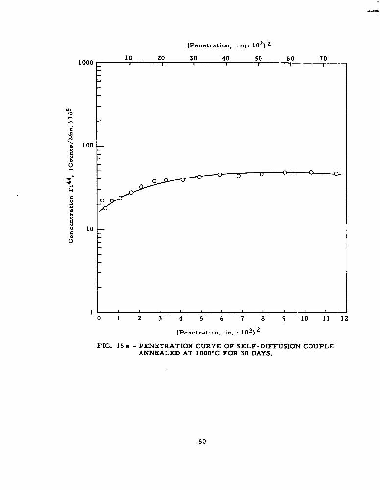
15e Penetration Curve of Self-Diffusion CoupleAnnealed at 10000C for 30 Days ..... ............
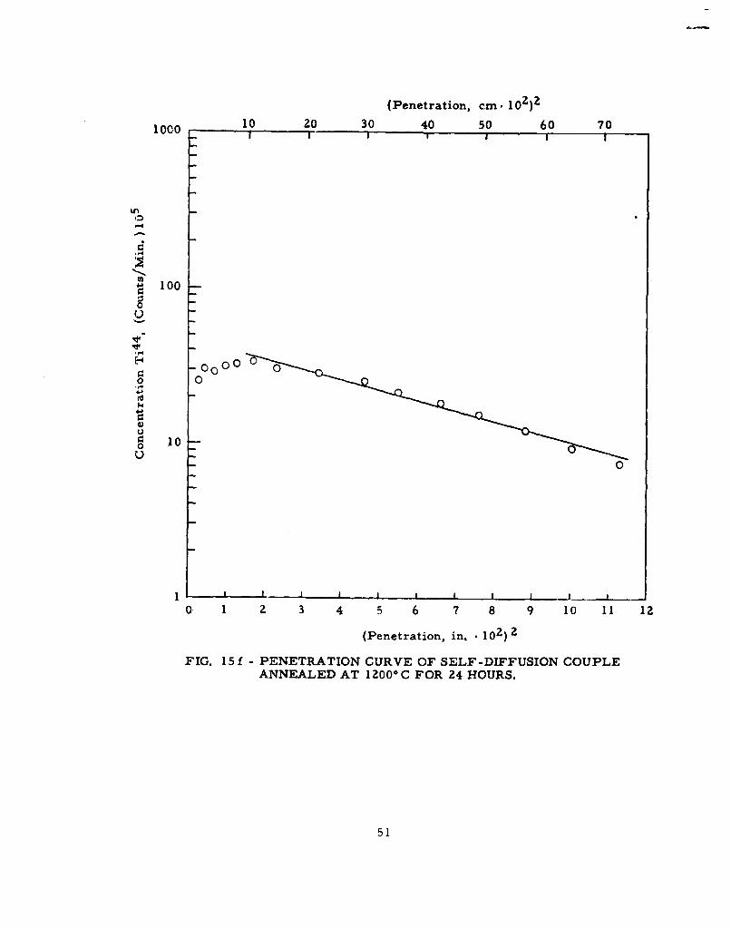
15f Penetration Curve of Self-Diffusion Couple 51Annealed at 1200*C for 24 Hours .........
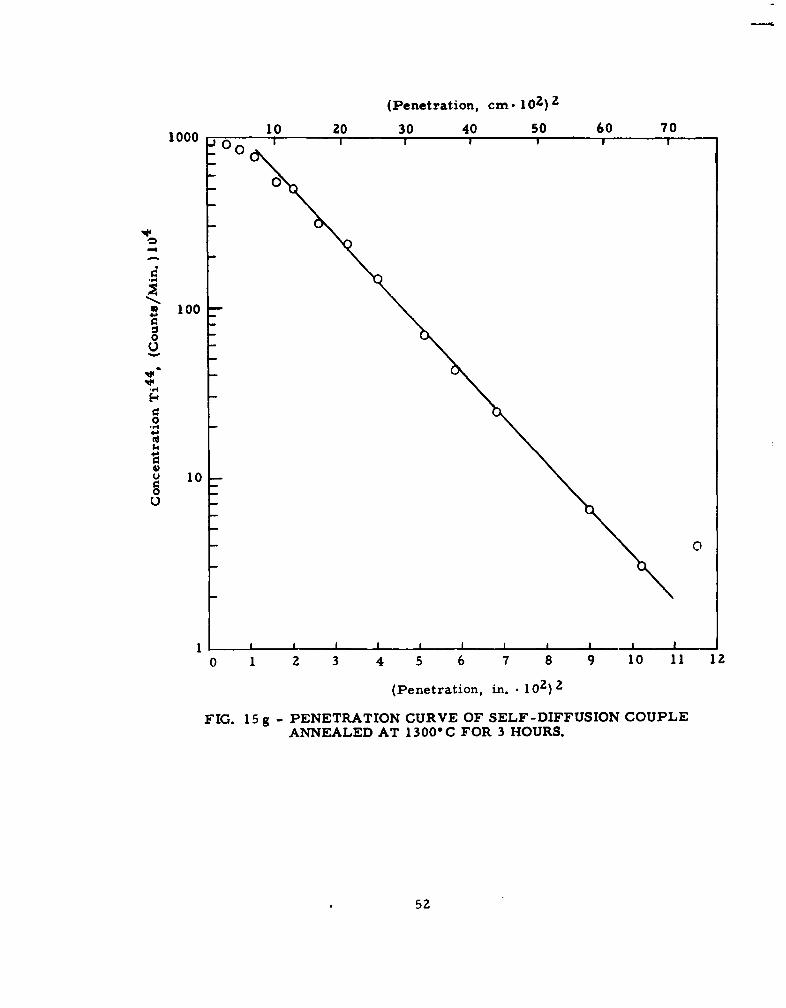
15g Penetration Curve of Self-Diffusion Couple 52Annealed at 13000C for 3 Hours.. ...........
16 Summary of Self-Diffusion Coefficients for Titanium. 53
vi
LIST OF TABLES
Table Page
I Summary of Interdiffusion Studies ......... ............ 22
II Materials Used in Production of Alloys ....... .......... Z3
III Microprobe Standards .............. ................. 24
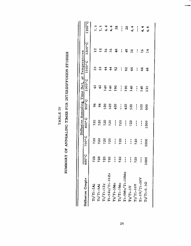
IV Summary of Annealing Times for Interdiffusion Studies 2 . Z5
V Summary of Calculated Interdiffusion Coefficients ..... ... 26
VI Summary of Calculated Self-Diffusion CoefficientsFor Titanium .................... .................... Z7
viu
DIFFUSION IN TITANIUM AND
TITANIUM ALLOYS
L INTRODUCTION
Diffusion characteristics, atom mobility, and activation energy arebasic to all metal processes which involve: (a) the movement of crystalfaults; (b) the kinetics of alloy transformation; or (c) .he development ofcomposite structures such as clads and laminates. The lack of adequatediffusion data for titanium-based alloys has hampered correlation of knownphysical phenomena such as nucleation, growth, age hardening, and themartensitic transformations of these alloys with what is probably the con-trolling factor. It is therefore both scientific and practical to analyze thediffusion characteristics of titanium and titanium alloys.
IL LITERATURE SURVEY
To date, little information is available on the diffusion of secondmetals in titanium, although a fair amount of data is available on inter-stitial diffusion in titanium. The Titanium Metallurgical Laboratory, inReport No. 21 and a subsequent Memorandum (1, 2), has reviewed both theopen literature and Government publications. More recently Peterson (3)has published a critical review of diffusion data for refractory alloys.
Due to the general belief that there is no suitable radioactive isotope,no self-diffusion data for titanium are available in the literature. Theactivation energy for self-diffusion has been estimated.
a. An activation energy of 73. 600 cal/mol is calculated fromthe equation of LeClai,.. (4).
b. Peterson (3) has plotted the activation energy for self-diffusionvs melting temperature from which a value of 72, 20O cal/molis estimated.
c. Nachtrieb and Handler (5) show the relationship betweenlatent heat of fusion, melting temperature, and activationenergy of self-diffusion. From this formula, a value of73, 600 cal/mol is calculated by Peterson (3) for P-Ti.Peterson (3) quotes Kaufman, who has calculated a meltingtemperature of a-Ti to be approximately the same as P-Ti.From this it is concluded that the activation energy of self-diffusion of a- and P-Ti would be approximately the same.
Manuscript released by the author March 1962 for publication as an ASDTechnical Report.
I
d. Reynolds, Ogden, and Jaffe (6) have inferred the activationenergy for self-diffusion of titanium to be approximately75, 300 cal/mol, based on an hypothesis formed for the aircontamination of commercial titanium sheet.
e. Orr, Sherby, and Dorn (7) have calculated the activationenergy of self-diffusion to be 60, 000 cal/mol from creepstudies. Dorn (8) has shown that activation energy forcreep is identical with the activation energy for self-diffusion.
f. Polonis and Parr (9) have estimated an activation energy ofself-diffusion of titanium to be 77, 000 cal/mol based on astudy of decomposition kinetics of titanium-nickel alloys.
Kidson and McGurn (10) have recently determined the self-diffusioncoefficient of P-zirconium and show that the observed activation energy isabout one half that calculated by such indirect methods as those obtained bythe above-listed investigators. Kidson and McGurn cite similar evidencethat the activation energy for self-diffusion of y-uranium, p-titanium, andchromium is about half that calculated by indirect methods. Pound, Bitler,and Paxtun (11) have suggested an explanation of such a phenomenon.
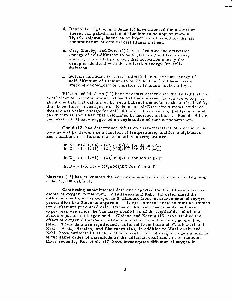
Goold (12) has determined diffusion characteristics of aluminum inboth a- and P-titanium as a function of temperature, and for molybdenumand vanadium in P-titanium as a function of temperature:
In DT = (-11. 04) - (23, 700)/RT for Al in a-Tiln DT = (-ll. 11) -(21,900)/RT for Al in P-Ti
In DT = (-11. 51) - (24,'000)/RT for Mo in P-Ti
in DT = (-5. 12) - (39, 600)/RT for V in P-Ti
Martens (13) has calculated the activation energy for zi:'conium in titaniumto be 23, 000 cal/mol.
Conflicting experimental data are reported for the diffusion coeffi-cients of oxygen in titanium. Wasilewski and Kehl (14) determined thediffusion coefficient of oxygen in P-titanium from measurements of oxygenpenetration in a Sieverts apparatus. Large external scale in similar studiesfor a-titanium precluded calculations of diffusion coefficients by theseexperimenters since the boundary conditions of the applicable solution toFick's equation no longer held. Claisse and Koenig (15) have studied theeffect of oxygen diffusion in P-titanium under the influence of an electricfield. Their data are significantly different from those of Wasilewski andKehl. Pratt, Bratina, and Chalmers (16), in addition to Wasilewski andKehl, have estimated that the diffusion coefficient of oxygen in a-titanium isof the same order of magnitude as the diffusion coefficient in P-titanium.More recently, Roe et al. (17) have investigated diffusion of oxygen in
2
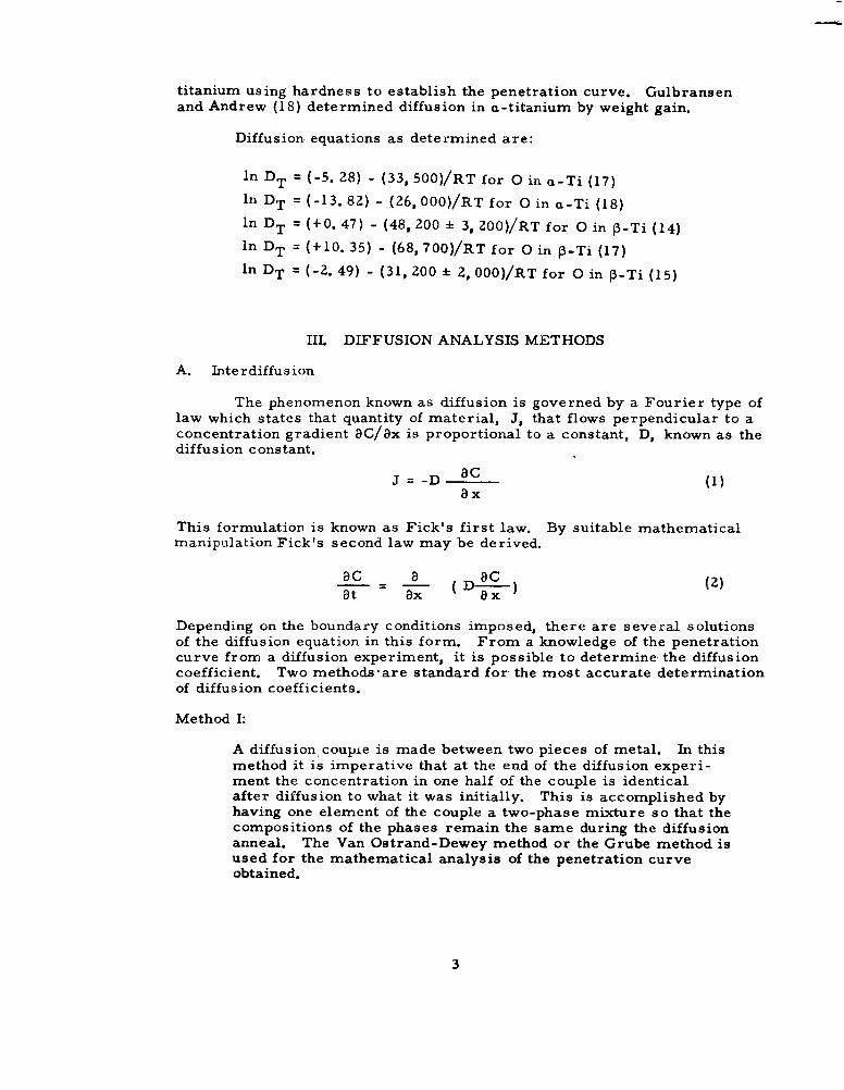
titanium using hardness to establish the penetration curve. Gulbransenand Andrew (18) determined diffusion in a-titanium by weight gain.
Diffusion equations as determined are:
In DT = (-5. 28) - (33, 500)/RT for 0 in a-Ti (17)
in DT = (-13. 82) - (26, 000)/RT for 0 in a-Ti (18)
in DT = (+0. 47) - (48, 200 ± 3, 200)/RT for 0 in P-Ti (14)in DT = (+10. 35) - (68, 700)/RT for 0 in P-Ti (17)
In DT = (-2. 49) - (31, 200 + 2, 000)/RT for 0 in P-Ti (15)
III. DIFFUSION ANALYSIS METHODS
A. Interdiffusion
The phenomenon known as diffusion is governed by a Fourier type oflaw which states that quantity of material, J, that flows perpendicular to aconcentration gradient GC/8x is proportional to a constant, D, known as thediffusion constant.
J =-D aC (1)ax
This formulation is known as Fick's first law. By suitable mathematicalmanipuIlation Fick's second law may be derived.
aC 8 DCat - x (D----) (2)
Depending on the boundary conditions imposed, there are several solutionsof the diffusion equation in this form. From a knowledge of the penetrationcurve from a diffusion experiment, it is possible to determine the diffusioncoefficient. Two methods-are standard for the most accurate determinationof diffusion coefficients.
Method I:
A diffusion. couple is made between two pieces of metal. In thismethod it is imperative that at the end of the diffusion experi-ment the concentration in one half of the couple is identicalafter diffusion to what it was initially. This is accomplished byhaving one element of the couple a two-phase mixture so that thecompositions of the phases remain the same during the diffusionanneal. The Van Ostrand-Dewey method or the Grube method isused for the mathematical analysis of the penetration curveobtained.
3
Method II:
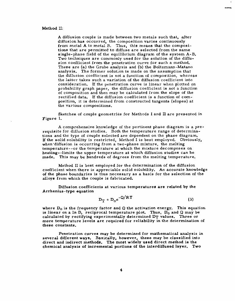
A diffusion couple is made between two metals such that, afterdiffusion has occurred, the composition varies continuouslyfrom metal A to metal B. Thus, this means that the composi-tions that are permitted to diffuse are selected from the samesingle-phase field of the equilibrium diagram of the system A-B.Two techniques are commonly used for the solution of the diffu-sion coefficient from the penetration curve for such a method.These are (a) the Grube analysis and (b) the Boltzmann-Matanoanalysis. The former solution is made on the assumption thatthe diffusion coefficient is not a function of composition, whereasthe latter takes such a variation of the diffusion coefficient intoconsideration, If the penetration curve is linear when plotted onprobability graph paper, the diffusion coefficient is not a functionof composition and then may be calculated from the slope of therectified data. If the diffusion coefficient is a function of com-position, it is determined from constructed tangents (slopes) atthe various compositions.
Sketches of couple geometries for Methods I and II are presented inFigure 1.
A comprehensive knowledge of the pertinent phase diagram is a pre-requisite for diffusion studies. Both the temperature range of determina-tions and the type of couple selected are dependent on the phase diagram.If the solid solubility is restricted, Method I is best employed. Obviously,when'diffusion is occurring from a two-phase mixture, the meltingtemperature--or the temperature at which the mixture decomposes onheating--limits the upper temperature at which diffusion studies can bemade. This may be hundreds of degrees from the melting temperature.
Method II is best employed for the determination of the diffusioncoefficient when there is appreciable solid solubility. An accurate knowledgeof the phase boundaries is thus necessary as a basis for the selection of thealloys from which the couple is fabricated.
Diffusion coefficients at various temperatures are related by theArrhenius-type equation
DT = Doe-Q/RT (3)
where Do is the frequency factor and Q the activation energy. This equationis linear on a In D, reciprocal temperature plot. Thus, Do and Q may becalculated by rectifying experimentally determined DT values. Three ormore temperature levels are required for reliability in the determination ofthese constants.
Penetration curves may be determined for mathematical analysis inseveral different ways. Basically, however, these may be classified intodirect and indirect methods. The most widely used direct method is thechemical analysis of incremental portions of the interdiffused layer. Two
4
similar direct methodsbut requiring more extensive facilities for analysis,are radioactive tracer techniques and mass-spectroscopic analysis when astable isotope is used as a tracer. Recently, the microprobe analyzer hasbeen used to determine directly the penetration curves of diffusion couples.Since it is not necessary to divide the diffusion couple into a finite numberof increments, the latter method has the twofold advantage of being essen-tially a continuous penetration curve determination and permitting diffusionanalyses to be made where limitations of time and temperature do not allowan extended interdiffused zone to be established.
Indirect methods such as hardness and resistivity traverses acrossthe interdiffused layer can be used to plot the penetration curve. Inasmuchas these methods require additional experimental data to correlate thephysical property with the chemical composition, they should be used onlyas a last resort.
B. Self-Diffusion
The most direct method of determining the self-diffusion coefficientof a metal is by analyzing a diffusion penetration curve. The diffusion coupleso formed must employ an isotope of the metal to enable the penetration curveto be established. The most common method of accomplishing this is by useof a radioactive isotope and determining the penetration by autoradiographicor counting techniques. However, it is possible to use nonradioactive iso-topes and to use a mass spectrometer to analyze the diffusion couple.
Attempts have been made to approximate self-diffusion phenomenaby extrapolating binary diffusion data to infinite dilution. Thomas andBirchenall (19) found that this is not necessarily valid. They concluded:"The deviation of the diffusion coefficient at infinite dilution from the self-diffusion coefficient of the solvent metal is generally greater the greater themelting point depression. Both factors also tend to become greater the morelimited the solid solubility of the solute metal. "
Self-diffusion data have also been determined by indirect methods.Kuczynski (20, Z1) has theoretically analyzed the width of the bond in sinter-ing of fine wires and has shown that this varies as the fifth root of time.There are two objections to this method: (a) the theory is not proved;(b) reliable and reproducible data are almost impossible to obtain becauseof numerous other uncontrollable variables in the experimental technique.
Self-diffusion data for tungsten have been obtained by Muller (22) byobserving the change of shape of a pointed wire heated in a vacuum. Noindependent data are available to prove this method.
5
The concentration ;% constant temperature for an identifiable atommay be expressed by
_ exp (- -) (4)2 G nDt 4Dt
where C is the concentration of the atom at distance x from the initial pointafter time t. S is the initial concentration, and D is the self-diffusioncoefficient at the given temperature. This may be put in the form of thelinear equation
n )T i Dt 4Dt
The diffusion coefficient is readily solvable from the slope when the experi-mental data are plotted as concentration as a function of the square of dis-tance from the surface.
From the Arrhenius equation previously discussed, the jump frequencyDo and activation energy, Q, may be calculated from DT values determinedat various temperatures.
IV. EXPERIMENTAL PROGRAM
A. Selection of Alloys for InterdiffusionOf Al, Zr, Mo, V, and 0 in Titanium
The research program devised for the determination of diffusion ofaluminum, zirconium, molybdenum, vanadium, and oxygen in both alphaand beta titanium was the analysis of penetration curves of couples preparedby pressure welding. Couples consisted of either pure titanium with a dilutealloy of the element whose diffusion coefficient is to be determined, or oftwo dilute alloys of the element whose diffusion coefficient is to be deter-mined. In the case of molybdenum, zirconium, and vanadium, it would havebeen possible to determine the diffusion coefficients for all compositions byforming the couple between titanium and molybdenum, zirconium, orvanadium. Such a technique is to be avoided since--as has been demonstratedby Reynolds, Averbach, and Cohen (23)--the diffusion coefficients so obtainedare higher at a given alloy composition than a coefficient determined at thesame alloy composition but from a couple of less severe concentrationgradient. The increased diffusivity is rationalized as a result of strainsassociated with the concentration gradient. To minimize the effect of com-position gradient strains on the diffusion coefficient, the compositiongradients were kept at a minimum.
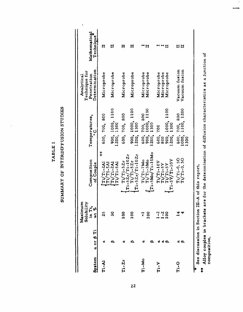
A surnma-y of the experimental work for the determination of inter-diffusion coefficients is given in Table L In instances where there is anextended solid solubility two couples were prepared: unalloyed titaniumbonded to a titanium alloy containing 5% zirconium--designated Ti/Ti-5Zr--and a bonded couple of 5 and 10% Zr alloys--designated Ti-5Zr/Ti-l0Zr.
6
By such a technique it is possible to determine the diffusion coefficient ofzirconium over a wide compositional range without undue strain effects.
It is appropriate to make a few pertinent comments with regard tothe selection of the experiments listed in Table L In general, alloyingadditions to commercial titanium alloys are under 10 per cent, but greaterthan 1 per cent. Consequently, the experimental program is designed toprovide diffusion data as a function of composition up to 10 per cent.
Beta titanium is continuously soluble with zirconium, molybdenum,and vanadium. The solubility of aluminum in P-titanium is extensive. Con-sequently these alloys are ideally suited for diffusion couples producing acontinuous penetration curve. Method II is the mathematical technique.Similarly, the solubility limits of aluminum and zirconium in alpha titaniumenable these techniques to be employed.
The limited solubility of molybdenum and vanadium in alpha titaniumdictate that experimental procedures and mathematical techniques of Method Ibe selected. It is possible that Method II could be used by fabricating acouple of titanium with a very dilute alloy (e. g. , Ti/Ti-0. 25Mo); however,the lack of precision with which the equilibrium diagram is known near theallotropic temperature would make it questionable whether the elements ofthe diffusion were in the single-phase field.
Since oxygen in titanium alloys exists principally as a contaminant,a much more restricted composition has been selected for a diffusion couple.The extended solubility of oxygen in both alpha and beta titanium enableMethod II to be used.
B. Selection of Geometry for Study ofSelf-diffusion of Titanium
As has been previously discussed, only tracer techniques can berelied upon to give accurate self-diffusion data. For this reason, a radio-active tracer technique was selected for the determination of the self-diffusionof titanium.
Four radioactive isotopes of titanium are known. These with theirrespective half-lives are: Ti 4 3 , 0. 6 seconds; Ti 4 4 , >1000 years- Ti453. 08 hours; and Ti 5 1 , 5. 80 minutes. The half-lives of all but Ti are tooshort to enable them to be fabricated into a diffusion couple and subsequentlyto be annealed. Thus Ti 4 4 is the only practical isotope by which diffusionexperiments can be performed.
Recently, it was reported (24-26) that if scandium is bombarded withdeuterons or protons in a cyclotron, a portion of the scandium is convertedto Ti 4 4 . This isotope has a half-life of 1000 years. The activity of theproduct is l05 disintegrations per minute. By conventional chemical tech-niques it is possible to separate the radioactive titanium from the scandium.However, because of the tiny amount of radioactive titanium present in thebombarded sample, microchemical techniques are necessary to preventdilution beyond a useful radioactive level. To maximize detection sensitivity
7
in the determination of the self-diffusion gradient, it is imperative that thespecific activity of titanium be reduced as little as possible by the additionof the non-radioactive carrier in the chemical processing.
Couples for the determination of the self-diffusion of titanium can bemade by two techniques: (a) reducing Ti 4 4 -enriched titanium to metallictitanium, which can be vapor-deposited on a non-radioactive titanium base,or (b) depositing Ti 4 4 -enriched TiO2 on a non-radioactive titanium surfaceand permitting the oxide to dissolve.
Procedure (b) is feasible since the total amount of oxygen added willbe negligible or, at most, the same order of magnitude as the residualoxygen in the titanium. Inasmuch as the diffusion of oxygen is expected tobe much greater than the self-diffusion of titanium, the localized concentra-tion at the interface will be existent only for a very short time. By such aprocedure the need for, the microchemical reduction of a titanium salt iscircumvented. A second advantage of such a procedure is that 100% of theminute quantity of radioactive titanium can be utilized by this technique ascontrasted to vapor deposition.
C. Production and Analysis of Diffusion Couples
1. Preparation of Alloys
Melts weighing 150 grams were prepared in a nonconsumable electrodearc furnace. The compositions of alloys are listed as part of Table L Ininstances it was necessary to make more than one alloy of a given composi-tion so that enough stock could be prepared for the required couples. High-purity components, as shown in Table II, were used in the alloy charges.
The dilute oxygen alloy was prepared through an intermediary masteralloy step. The high-purity TiO2 was pressed and sintered at 1000°C priorto being used in preparing a 5% master alloy.
For the preparation of the self-diffusion couples, a three-poundingot was melted.
In addition to the melts that were prepared for the manufacture ofdiffusion couples, a series of ten-gram ingots were melted as standards forthe microprobe study. The compositions of these standards are given inTable III, along with spot chemical analysis. In all cases the chemicalanalyses deviate systematically from the nominal composition. Inasmuchas no weight losses were experienced in the melting, the nominal composi-tion was subsequently used. The deviation from the nominal in the chemicalanalysis is attributed to the analytical method.
Z. Preparation of Interdiffusion Couples
Alloys containing aluminum, zirconium, molybdenum, and vanadiumwere fabricated into plate 1/4 inch thick by hot rolling at a temperature 100* Cbelow the P/a + P transus. Approximately fifty minutes were accumulatedin the rolling process. The rolling temperatures are tabulated as follows:
8
Ti 675°CTi-ZAl 8000Ti-5AI 8250Ti-5Zr 750"Ti-l0Zr 750°Ti-5V 7000Ti-10V 650"Ti-5Mo 750°Ti-7Mo 725"Ti-lOMo 700"
Samples 1 x 1 1/2 inches were cut from the rolled plate. Thesewere then ground to 1/8 inch thick specimens by removing an equal amountof stock from opposite sides of the rolled plate. This scalping operationwas more than sufficient to remove the contamination arising from processingin air. * The faces were then lapped to flatness by an automatic lapper.After lapping, the surfaces were thoroughly washed with petroleum etherfollowed by acetone. Surfaces were then etched with a solution composed of60 cc HNO 3 , 10 cc HF, 30 cc H2 0.
Roll bonding was found to be a convenient and satisfactory method toproduce the bonding required for the diffusion couples. Samples to be rollbonded are encapsulated in a stainless steel container as shown in Figure Z.Prior to evacuation the container is given a very light cold reduction to pre-vent members of the couple from sliding out of position. The sealed unit isheated to 9500 C for 15 minutes and given a one-pass 2016 reduction. Thecapsule is then permitted to cool below 600 C and water quenched. It wassubsequently established that the diffusion effect occurring during rollingwas less than a detectable amount.
Several compositions could not be roll bonded until titanium spongewas introduced into the stainless steel envelope to insure complete gettering.
Specimens 5/16 inch square were sawed from the bonded plate. Atotal of 18 specimens was produced from the single roll-bonding operation.
The alloys containing oxygen were processed slightly differentlyfrom those described above. The ingots were rolled to slab 0. 42 inch thickwhich was subsequently milled and lapped into plate 0. 30 inch thick.Inasmuch as oxygen penetration must be determined by direct chemicalanalysis, the size of the interface must be larger and the planeness of theinterface more accurately controlled. Roll bonding techniques did not per-mit a sufficiently flat interface to be produced. By hot pressing, the rippleof the interface was greatly reduced. Slabs of the alloy were canned andpress bonded at 950° C with a reduction of - 32%6. Eight couples, eachmeasuring 1/2 x 3/4 inch,were cut from two bonded specimens measuring1 1/2 x 2 inches. The variation of the interface was determined to be-0. 008 inch from photographs of the four sides of the 1/2 x 3/4 inch speci-mens. Diffusion minimizes the effect of the initial variation of the interface.Inasmuch as the machined layers for the penetration curve analysis were ofthe order of 0. 015 inch thick, this initial variation is insignificant.
* This problem has been discussed by Reynolds, Ogden, and Jaffee (27).
9
3. Preparation of Self-diffusion Couples
The specimen designed for production of self-diffusion couples byabsorption of Ti 4 4 -enriched TiO2 is shown in Figure 3. A water susperf-sion of TiOz is placed in the cavity at the top and permitted to settle intoan even layer at the bottom. The water is permitted to evaporate. Thespecimen is then heated to calcine the TiO2 and is subsequently given therequisite diffusion anneal. After diffusion annealing, but prior to section-ing into layers, the specimen is turned to 3/8 inch diameter to eliminateeffects of non-planar diffusion at the corners and to remove any irregular-ities due to unevenness of the precipitated TiO 2 layer at the corners.
The three-pound arc-melted ingot of titanium was forged to a one-inch round bar and subsequently machined into specimens of dimensionsshown in Figure 3.
The Nuclear Science and Engineering Company of Pittsburgh, Pa.,were contacted, and they agreed to undertake the production of Ti 4 based.on the literature that was supplied to them. All subsequent investigationsof self-diffusion have been based on a total quantity 6f 0. 010 grams titanium(0. 016 grams TiO 2 ) acting as carrier for the Ti 4 4 . It was decided thattwelve specimens would be produced, one each for eight temperatures andfour spares.
Prior to the actual production of the working self-diffusion couples,the precipitation and absorption characteristics of TiO2 were thoroughlyevaluated.
A suspension of 0. 016 gram TiO2 in a quantity of water twelve timesthe cavity volume of Figure 3 was prepared. The TiO2 tended to coagulateand form a very uneven deposit on settling. If, however, a tiny amount ofAlconox (a commercial wetting agent) is added, a smooth, even deposit canbe produced on settling. By serial dilution experiments it was establishedthat an 0. 02% solution of Alconox was the minimum amount that wasnecessary to obtain the type of deposit desired.
Using an 0. 02% solution of Alconox, the absorption characteristicsof TiO2 were investigated at 600%, 8000, 900, and 1000*C. Completeabsorption of the oxide was obtained under the following conditions:
1000 0 C 1 hr9000C 10 hr8000C 83 hr6000 C undetermined
Similar absorption experiments were carried out for oxide suspen-sions that contained no Alconox wetting agent; the times required to dissolvethe oxide were the same as above.
Details of the chemical methods used by the Nuclear Science andEngineering Corporation for the production of Ti 4 4 -enriched TiO2 areincluded in Appendix L
10
4. Diffusion Annealing
Data contained in the review by Peterson (3) was used as a basisfor the selection of annealing times at the various temperatures.
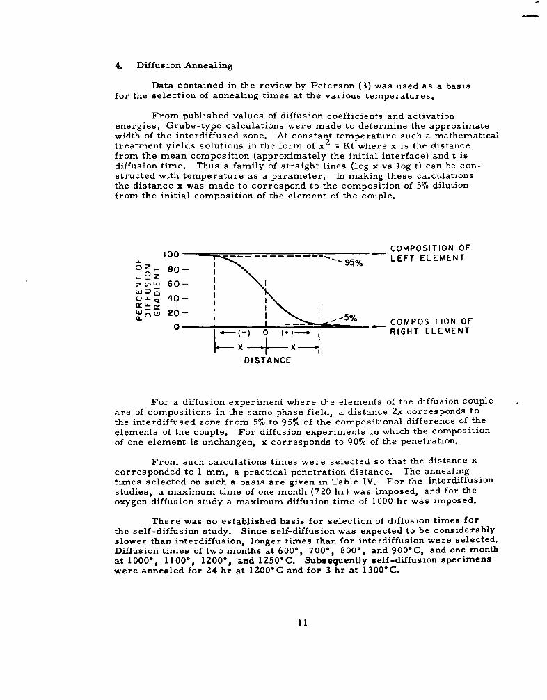
From published values of diffusion coefficients and activationenergies, Grube-type calculations were made to determine the approximatewidth of the interdiffused zone. At constant temperature such a mathematicaltreatment yields solutions in the form of x2 = Kt where x is the distancefrom the mean composition (approximately the initial interface) and t isdiffusion time. Thus a family of straight lines (log x vs log t) can be con-structed with temperature as a parameter. In making these calculationsthe distance x was made to correspond to the composition of 5% dilutionfrom the initial composition of the element of the couple.
COMPOSITION OFU. 1 '''LEFT ELEMENT
zu uj 60-O
W DU 20-
_____ .- % COMPOSITION OF0 .0I_. .. ._ ,,_ _ --
- +RIGHT ELEMENT
DISTANCE
For a diffusion experiment where the elements of the diffusion coupleare of compositions in the same phase fielL, a distance 2x corresponds tothe interdiffused zone from 5% to 95% of the compositional difference of theelements of the couple. For diffusion experiments in which the compositionof one element is unchanged, x corresponds to 90% of the penetration.
From such calculations times were selected so that the distance xcorresponded to 1 mm, a practical penetration distance. The annealingtimes selected on such a basis are given in Table IV. For the interdiffusionstudies, a maximum time of one month (720 hr) was imposed, and for theoxygen diffusion study a maximum diffusion time of 1000 hr was imposed.
There was no established basis for selection of diffusion times forthe self-diffusion study. Since self-diffusion was expected to be considerablyslower than interdiffusion, longer times than for interdiffusion were selected.Diffusion times of two months at 600, 700, 800, and 9006C, and one monthat 10000, 11000, 1200°, and 1250*C. Subsequently self-diffusion specimenswere annealed for 24 hr at 1200"C and for 3 hr at 1300°C.
11
5. Penetration Curve Analysis for Substitutional Solutes
The diffusion experiments of the substitutional solute elementsaluminum, molybdenum, vanadium, and zirconium were devised for thepenetration curve analysis by electron microprobe analysis. Such a devicebombards a metal specimen with a small beam of electrons -0. 001 mm indiameter. The scattered electrons and the characteristic X-radiation excitedin the specimen are then analyzed. The Cambridge model microprobe analyzerat Armour Research Foundation has provision for deflection of the electronbeam so that the distribution of elements in a small area ( -0. 3 mm square)can be displayed on cathode ray tubes.
A block diagram of the Foundation's microprobe analyzer is shownin Figure 4. Two recent publications (28, 29) by Foundation staff membersgive further details of its operation and outline typical metallurgical applica-tions.
Prior to microprobe analysis, diffusion specimens had to be preparedcarefully by metallographic techniques. The 5/16 inch square specimenswere hand ground to fit into the 1/4 inch diameter specimen holder of themicroprobe stage. The specimens were then mounted in Bakelite and givena metallurgical polish. Extreme care was observed that the polished surfacewas perpendicular to the interface. The flat sides of the specimens wereused as a reference plane to maintain this perpendicularity. The specimenwas broken out of the mount prior to microprobe measurements.
Microprobe specimens cannot be etched since the concentration at theplane of measurement is altered by such etching. The diffusion specimenmust be positioned accurately on the microprobe stage so that solute concen-tration perpendicular to the interface can be determined. Since the interfacecould not be observed microscopically, accurate positioning was initially aproblem. This difficulty was overcome by scribing a line perpendicular tothe diffusion interface. The specimen was aligned on a microhardness testerand the line scribed by moving the microhardness stage under a suitablediamond.
Since the maximum deflection of the microprobe beam is -0. 3 mm,it was necessary to reposition the specimen on the stage of the microprobeanalyzer in order to determine the complete penetration curve. To facilitatethe repositioning of the specimen a series of Knoop hardness impressionswere made parallel to the scribed line with the point of the Knoop impressionperpendicular to the scribed line. The distance between these fiducial markscould be measured accurately with the microprobe as the scribed line andKnoop hardness impressions can be readily observed on the scattered electronimage.
It was initially thought that the most expedient method of determiningthe penetration curves on the electron microprobe analyzer would be to drivethe electron beam slowly across the interdiffused zone, measuring the con-centration either photographically or by counting techniques. The electroniccircuits of the instrument were modified to provide such a drive. Such amethod was found to be impractical since the integrated time over a small
12
area was too small to eliminate the statistical counting errors. Consequently,the beam was positioned over a desired area and the concentration determinedby counting for 100 seconds. The beam was then deflected to another area,and again the concentration was determined by counting for 100 seconds.
Three reference specimens were incorporated in the microprobevacuum chamber--pure titanium and two standard specimens (see Table III)which had been water-quenched from the P-field. From these data thepenetration curve, as determined in counts, could be transcribed to composi-tion. The slight degree of nonlinearity of counts as a function of compositionis therefore compensated.
The calculated composition sometimes deviated from the known com-position of the elements of the couple. The penetration curve as determinedby the microprobe was considered to represent diffusion from the boundaryalloy conditions in the prepared couples. All subsequent calculations weremade on such an assumption.
Because of the high absorption of aluminum K. radiation by titanium,it is not possible to use the microprobe analyzer for diffusion studies ofaluminum in titanium. It was impractical to determine the penetration curveof the aluminum diffusion samples by chemical analysis because the samplesize was too small, having been selected for the microprobe technique.Attempts were made to determine the penetration curve by microprobeanalysis of titanium radiation and by microhardness traverses. Theseattempts were unsatisfactory.
The diffused zone for molybdenum and vanadium in a-titanium wasextremely narrow, making the establishment of the penetration curve subjectto considerable error. Because of the extremely narrow penetration zone thesolubility limits of molybdenum and vanadium could not be read from thepenetration curve. A search of constitutional literature indicated that theselimits are not known precisely. Inasmuch as it was necessary to know theselimits to solve the diffusion equation, these had to be approximated based onthe best literature data and consistent with the observed penetration curves.
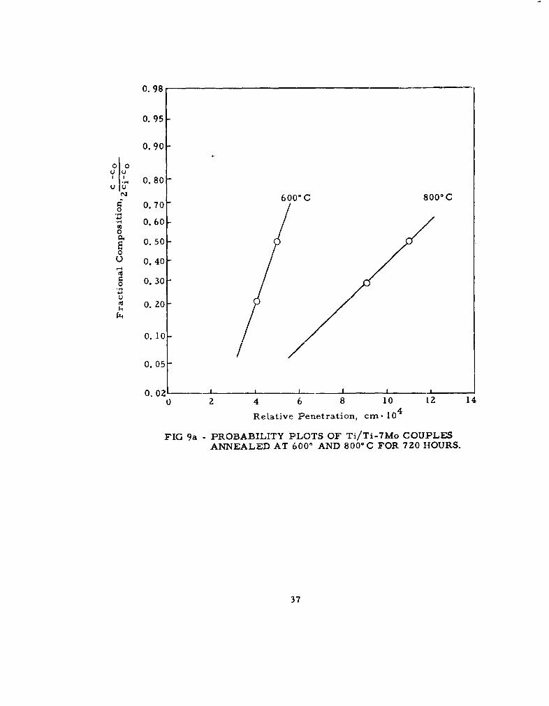
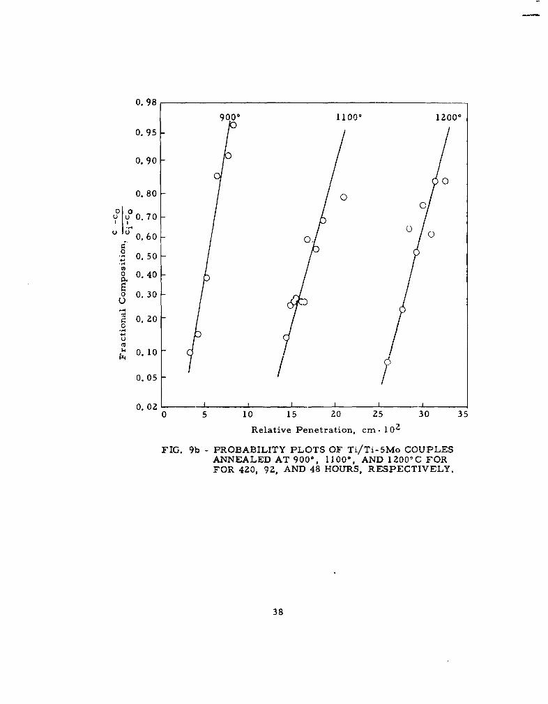
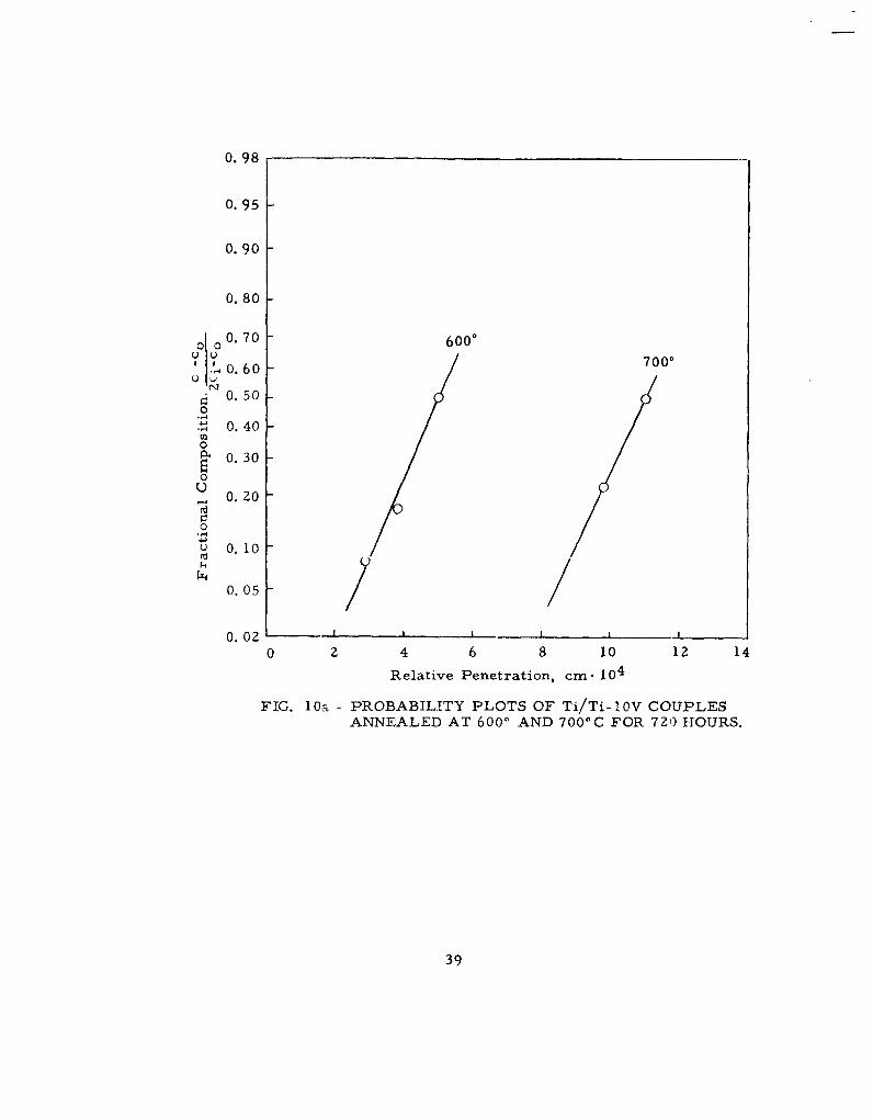
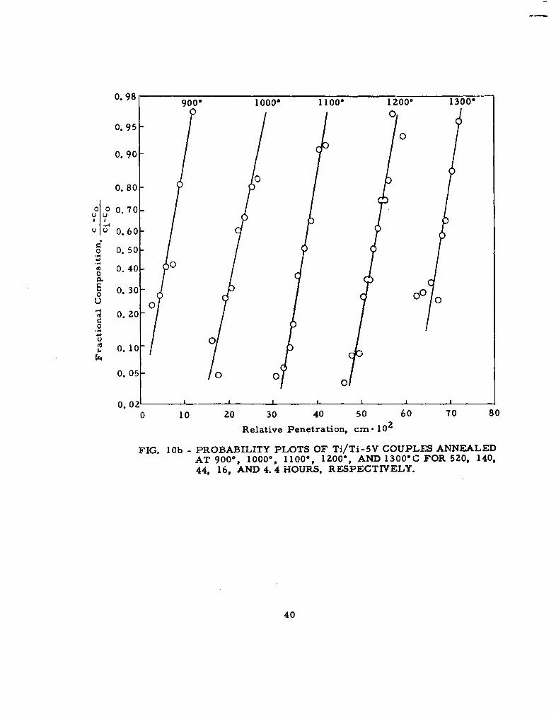
Typical penetration curves are given in Figures 5 and 6 for the diffusionof vanadium in a- and P-Ti, respectively. The rectification of these and otherdata have been by probability-distance curves as is shown in Figures 8 a and8b for zirconium, Figures 9 a and 9 b for molybdenum, and Figures l0 a andi 0 b for vanadium.
The linearity of the probability plots indicate that the diffusion coefficientis not a function of composition for the composition range investigated.
The mathematical solution of the diffusion equation may be expressedby:
' ( C -C -1 = erf( (6)ci-Co N(6
where (ci-co) is the diffusion gradient, c the composition at point x, measuredfrom the position where the error function (erf) is 50%; co anw.. ci are the
13
boundary compositions of the diffusion couple. A typical solution of thediffusion coefficient from rectified data is given in Appendix IL Deviationsfrom linearity of data at the extremes of probability plots according to thework of Johnson (30) are a result of inaccuracies of the chemical analysesand consequently should be ignored in constructing the best straight-line fitprior to making the mathematical calculation of the diffusion coefficient.
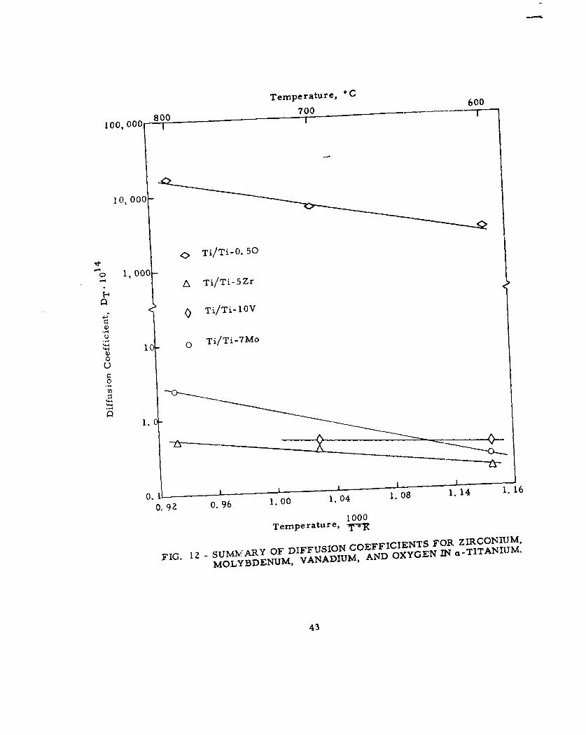
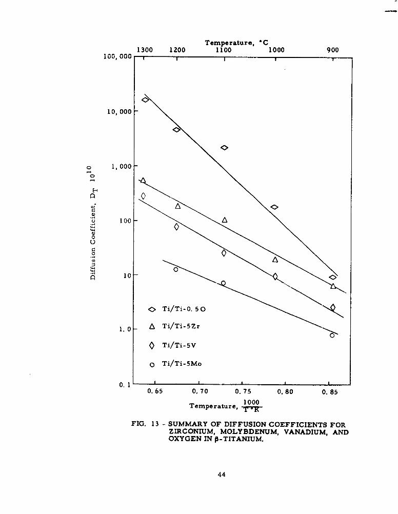
Calculated diffusion coefficients are summarized in Table V. Thelogarithms of these coefficients were then plotted as a function of reciprocaltemperature (Figs. 12 and 13) from which least-squares solutions were made.For systems where the diffusion coefficients were determined at three ormore temperatures, the standard errors in In Do and Q were calculated bystandard statistical analysis methods.
In DT = (-27. 14 + 1. 56) - (11, 800 ± 3, 000)/RT for Zr in a-TiIn DT (-4. 01 * 1. 22) - (40, 100 + 3, 300)/RT for Zr in p-Ti
In DT = (-17. 19) - (28, 400)/RT for Mo in a-TiIn DT = (-9. 00 + 0. 92) - (33, 100 + 2, 400)/RT for Mo in P-Ti
In DT = (-31. 39) - (3, 100)/RT for V in a-TiIn DT = (-4. 38 ± 1. 04) - (41, 400 * 2, 800)t/RT for V in P-Ti
6. Penetration Curve Analysis for Oxygen Diffusion
Penetration curves for the diffusion of oxygen in titanium weredetermined by vacuum fusion analysis of machined layers of diffusion couples.
The Ti-O diffusion couples were machined into layers by end milling.A specially designed fixture permitted collection of all machined chips with-out contamination. The thickness of the machined layer was calculated bythe difference in height from the reference surface. For specimens annealed900°-1300°C, layers 0.015 inch were machined; at the lower temperatures0. 015 inch cuts were made up to where the interface was, 0. 005 inch cutsthrough the diffused zone for 7000 and 8000 C specimens, and 0. 003 inch cutsfor the 6000C specimen. Alternate layers were analyzed by vacuum fusionanalysis. Prior to analysis, the machined chips were carefully washed withacetone.
The penetration curves showed the classical shape--for the mostpart, being smooth curves with a minimum of fluctuation. However, theend values were at considerable variance from the nominal, unalloyedtitanium and Ti-0. 5 wt % 0. The analyzed compositions of the elementswere subsequently determined: 0. 0229% and 0. 394% oxygen in the as-bondedcondition, and 0. 0289% and 0. 400% in the as-melted and rolled state.
It was initially thought that the increase in oxygen after diffusionannealing was attributable to contamination on the surface. Consequently,a 0. 030 inch layer was machined from the sides prior to machining intolayers. Except at the lower temperatures this removal had no appreciableeffect on the analysis since, for the diffusion times required, the contamina-tiondiffuases almost completely through the specimen.
14
Terminal compositions as established by the penetration curvesvaried from the original composition limits. Since this variation was morepronounced at the elevated temperatures, there can be no question but thatthis is attributable to contamination during annealing. In making themathematical analysis, it is assumed that the limits of the penetrationcurve as analyzed represent diffusion between the limits of the originalcomposition, 0. 03 and 0. 40 wt % 0, respectively.
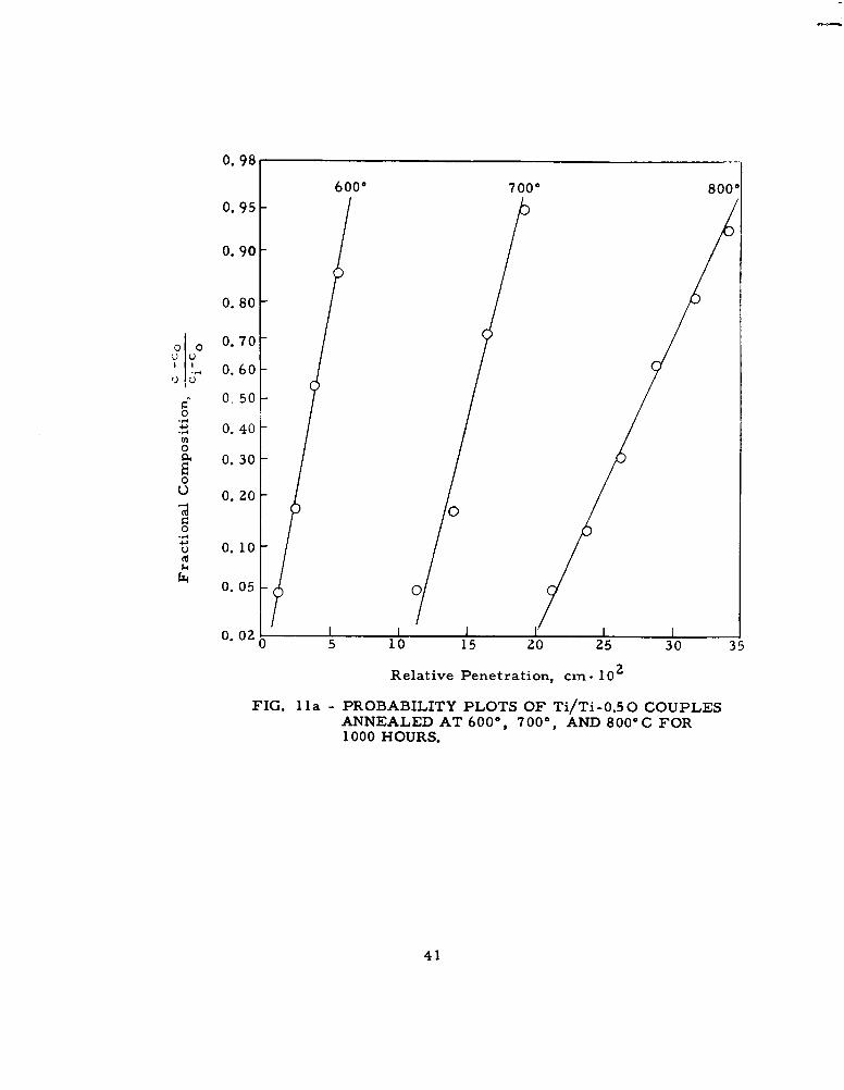
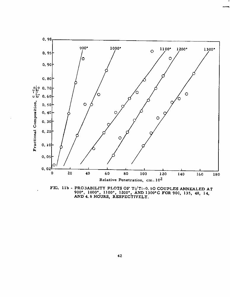
The mathematical solution and analysis of diffusion data for thedilute oxygen alloys is identical to that presented in the previous section.A typical penetration curve for oxygen is given in Figure 7. Probability-distance plots of the penetration data are shown in Figs. 11 a and 11 b whichyield diffusion coefficients summarized in Table V. By fitting these data tothe Arrhenius equation the following equations were obtained by least-squaressolutions and subsequent statistical analysis for the errors:
ln DT = (-14.94 * 1.15) - (16, 200 * 2, 200)/RT for 0 in a-Ti
ln DT = (+8. 37 * 2. 21) - (66,800 * 7, 000)/RT for 0 in A-Ti
7. Penetration Curves for Self-diffusion
The month-long anneals at temperatures above 10000C were impracti-cal for several reasons. First of all, at 12000 and 1250*C the quartz cap-sules devitrified resulting in deterioration of the specimen by oxidation.The specimens annealed at 1000* and 11000 C for one month deformed duringannealing by grain growth, distorting the planar geometry established forthe diffusion experiment. Finally, as was established on subsequent analysis,the time of annealing was far too long to permit a satisfactory gradient bywhich to calculate the diffusion coefficient.
As indicated by equations 6 and 7, machined layers must be taken atknown distances from the interface. The device used for machining the Ti-Odiffusion couples was satisfactorily employed in the preparation of machinedlayers of the self-diffusion couples. All measurements were made from thebottom surface as a reference plane. Layers were machined according tothe following schedule: 0. 000 (surface) to 0. 005 inch into 0. 001 inch thickincrements; 0. 005 to 0. 035 inch into 0. 002 inch thick increments for speci-mens annealed at 900 -1300°C; and 0. 005 to 0. 025 inch into 0. 002 inch thickincrements for specimens annealed at 600° -800* C. There was no need towash the machined chips since any slight oil contamination would not affectthe radioactivity analysis. The machining equipment, however, wasmeticulously cleaned between incremental cuts to prevent carryover ofradioactive chips. The weight of the machined chips was carefully measuredon a precision balance.
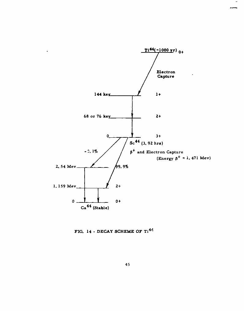
The decay scheme of Ti 4 4 has been described by Cybulska andMarquey (31), as shown in Fig. 14.
The activity of Ti 4 4 was measured by counting in a well-typeNaCl (Tl) crystal 1 3/4 inch diam. x 2 inches with a 3/4 inch diam., I inchdeep well. The crystal was contained in a low-background shielding system.
15
The titanium chips were contained in cellulose nitrate test tubes. Thecounter used was a Nuclear Data Corporation Model ND 130, 512 channelpulse height analyzer.
Two sets of data were •obtained. First, by setting the lowercriminator to a low value the activity of both Ti 4 4--> Sc• 4 and Sc 4 4 -- > Ca4
were obtained. Secondly, by setting the discriminator to approximately150 key, only the Sc 4 4 -- > Ca 4 4 activity was obtained. These measurementswere proportional. The former was used in plotting the penetration curves.Background measurements were taken for correction purposes. Activitywas measured for at least one minute, or for a sufficient time interval forover 10, 000 counts. In some instances, counting times up to one hour werenecessary. Because of the intensity of the activity, the error due to countingis extremely small--from less than 1% for the great bulk of the readings toapproximately 3% for some of the very weak activity measurements.Weighing and distance measurement errors are by far the prime source oferror in establishing the penetration curve.
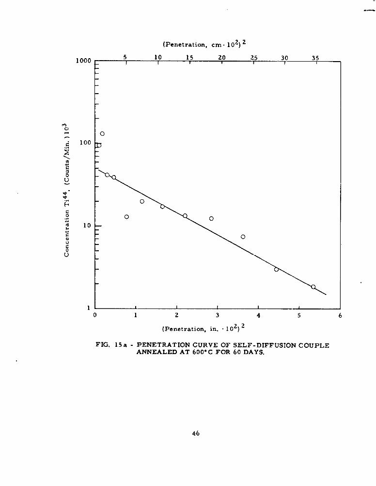
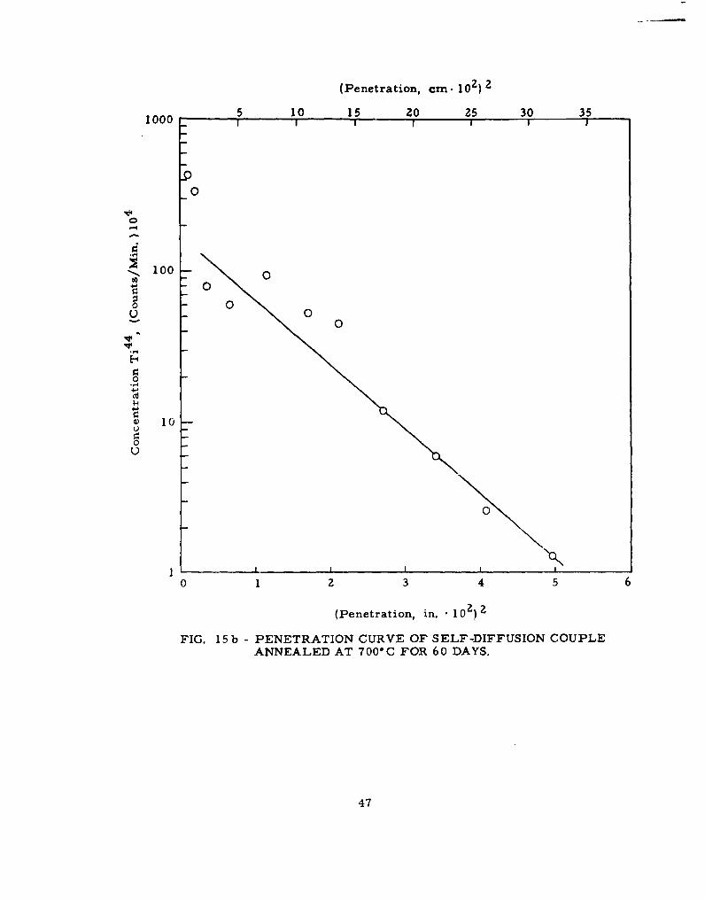
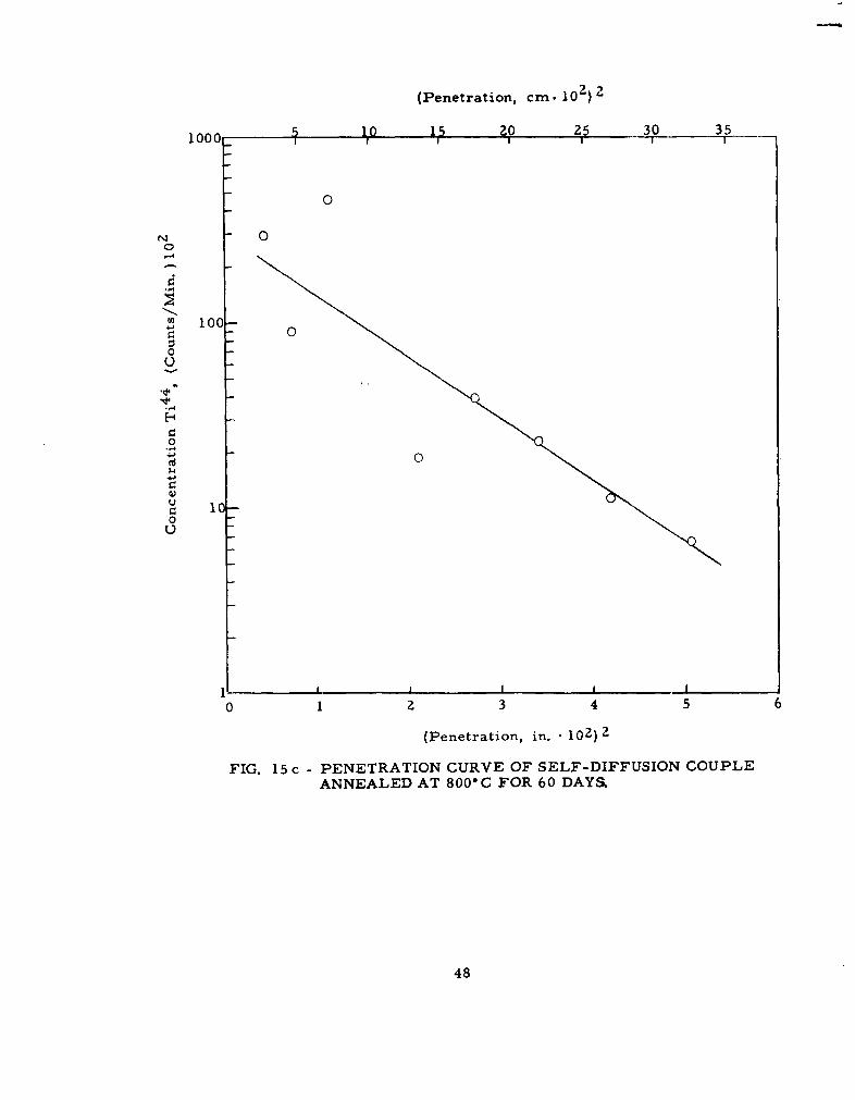
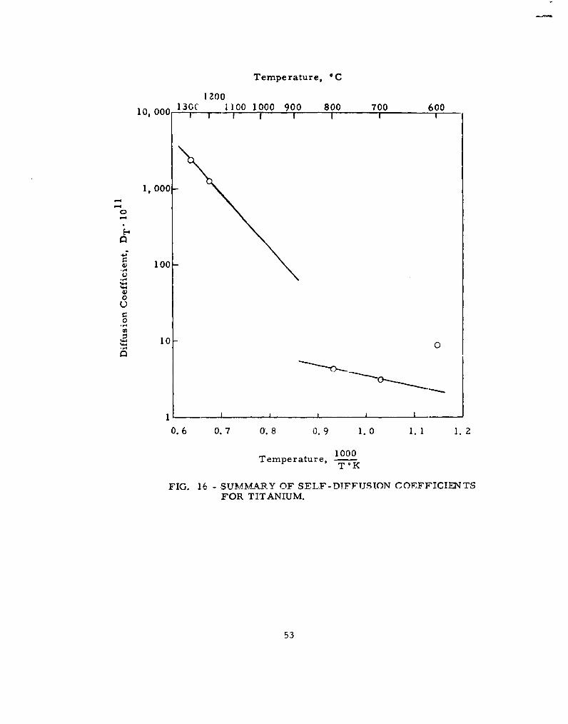
The specific activity is obtained by dividing the activity rate by theweight of the specimen. Penetration curves for the self-diffusion of titaniumare presented in Figs. 15a-15g for 600% 700', 800, 9000, 10000, 12000,and 1300°C. Only those curves at 600, 700% 800, 1200, and 13000Care amenable to diffusion calculations. The calculated diffusion coefficientsare summarized in Table VL
The diffusion coefficients have been plotted as log D-reciprocaltemperature in Fig. 16. Fromthis it is at once seen that the diffusioncoefficient at 6000C is non-consistent with the data of 7000 and 8000C.The datum at 600° was not used in making the frequency factor Do andactivation energy calculations.
The self-diflusion data permit the following equations to be evaluated:
In DT = (-21. 08) - (5, 700)/RT for a-TiIn DT = (-8. 40) - (28,600)/RT for P-Ti
V. DISCUSSION
The use of the electron microprobe analyzer has proved to be anexcellent and most reliable tool in the determination of interdiffusion gradients.However, even such a facile tool has limitations as was found in the case ofthe detection of interdiffusion of aluminum in titanium. The use of such aninstrument enables the accurate delineation of a diffusion gradient that couldnot be done by conventional chemical analysis techniques. There was noprevious experience of prior workers on which to draw in planning the experi-ments for the microprobe analysis. With one exception the techniquesdeveloped were very good; it is recommended that means be incorporated irothe sample to identify the original interface. Tungsten wires or thoria powderwould be expected to serve extremely well as such means.
16
The calculation of diffusion constants for oxygen in titaniumpresented in this investigation is the first instance in which the fundamentaldiffusion geometry was used and penetration curves established by directchemical analysis. The diffusion data for oxygen in both a- and P-titaniumwere classical; the penetration curves were smooth with a minimum amountof deviation. The diffusion coefficients were consistent with the Arrheniusrelationship. The minor contamination some specimens experienced at thehigh annealing temperatures should not have affected the results deleteriously.
The present investigation represents the first use of a radioactiveisotope of titanium in metallurgical research. It is unfortunate that theannealing times chosen were too long to enable significant constants to becalculated at most temperatures. However, the data so obtained in thisinvestigation tend to support observations made by Kidson and McGurn (10)for zirconium that the activation energy for self-diffusion determined directlycan be much lower than that determined by indirect means.
The jump frequency, DO, and the activation energy, Q, of the diffusionequation
DT = Doe Q/RT
must be solved from data obtained at several temperatures. A maximum offive data were available for a statistical analysis of the errors of the con-stants of P-titanium; a maximum of three for a-titanium. This -:ertainly isnot ideal for a precise determination of the diffusion constants. Ideally,multiple determinations should be made at temperatures at 25° or 50 Cintervals rather than single determinations at 100°C intervals as wasnecessary by/the broad scope of the present investigation.
The standard errors associated with Arrhenius equation are in Q andIn Do. It is therefore difficult to express meaningfully the temperaturedependence of the diffusion coefficient with the associated errors in any otherthan the logarithmic form. The logarithmic form was consequently usedthroughout this report.
The errors of the constants of the Arrherius equation vary widely but,in general, are better for diffusion in P- rather than a-titanium. With theexception of molybdenum, the activation energies are within 10% for P-titanium; the errors in In DO are up to 30%. For a-titanium (in the twosystems that permitted statistical analysis) the error in In Do was less than10%, but the error in Q was as great as 25%. These observations point tothe great need for multiple data if precise diffusion data are desired. Duecaution must also be observed in the casual use of published diffusion data towhich no error limits have been affixed.
The diffusion equations determined in this investigation may becompared with those of Goold (12) for molybdenum and vanadium in P-titanium, and with Roe et al. (17) for oxygen in P-titanium:
17
in DT = (-9. 00 + 0. 92) - (33 100 * 2, 400)/RT for Mo in P-Ti (this report)In DT = (-I1. 51) - (21, 900)/RT for Mo in P-Ti (Ref. 12)
In DT =(-4. 38* 1. 04) - (41 4010 * 2, 800)/RT for V in P-Ti (this report)In DT = (-5. 12) - (39, 600)/RT for V in P-Ti (Ref. 12)
In DT = (+8. 37 :k 2. 21) - (66 800 L 7, 000)/RT for 0 in P-Ti (this report)in DT = (+10. 35) - (68, 700)/RT for 0 in p -Ti (Ref. 17)
The agreement of the data above with published data is indicative ofthe over-all quality of the data in the present investigation as limited by thenumber of determinations from which the constants in the diffusion equationwere calculated.
Several comments are pertinent with respect to the magnitude of theconstants for the diffusion equation calculated in this investigation:
(a) The values of Do for interdiffusion of zirconium and vanadium ina-titanium are several orders of magnitude smaller than generally observedfor refractory metals. It can well be argued that the relatively short diffusiontime prevented accurate data from being established for molybdenum, butsuch is not the case for zirconium. In diffusion couples of the latter elementin titanium smooth penetration curves were observed yielding diffusioncoefficients in accord with the Arrhenius equation. The low value of Do folzirconium adds credence to the preliminary data for vanadium. The observa-tion is worthy of further study from a mechanistic standpoint.
(b) LeClaire (32) suggests that Do for self-diffusion varies from 0. 1to 10 (In Do from -2. 3 to +2. 3). On this basis of standard, the preliminarycalculations of Do for the self-diffusion of titanium are small. Data for self-diffusion of refractory alloys summarized by Peterson (3) tend to supportthis observation; however, an extreme from Do = 6. 3 .10 7 (In Do = 18. 0) fortungsten to Do = 10-4 (In Do = -9.2) for chromium are also recorded byPeterson. From the literature data for other self-diffusion constants itappears that the calculated value for Do for self-diffusion of titanium is toosmall, although this can be ascertained with certainty after further deter-minations.
On the basis of the investigations conducted the following recommenda-tions are made:
(a) The methods that have been developed for the determination ofself-diffusion in titanium give every evidence of being practical. A redeter-mination of the self-diffusion of titanium is certainly justified.
(b) The interdiffusion of molybdenum and vanadium in ct-titaniumshould be redetermined by employing diffusion anneals of at least six monthsand with some inert marker at the interface.
18

(c) The accuracy of the diffusion constants of the alloying elementsin P-titanium and for oxygen and zirconium in a-titanium as calculated inthis investigation was limited by the number of evaluations of diffusioncoefficients and temperatures employed. If the calculated values of Q andDo are to be refined, it will be necessary to use a statistical approachthrough the use of a far greater number of individual diffusion couples.
19
REFERENCES
1. J. E. Reynolds and R. I. Jaffee, "The Diffusion of Interstitial andSubstitutional Elements in Titanium, " Titanium Metallurgical Laboratory,Report No. 21, October 25, 1955.
2. R. E. Maringer, "Solid State Diffusion in Titanium", Memorandum ofTitanium Metallurgical Laboratory, June 9, 1958.
3. N. L. Peterson, "Diffusion in Refractory Metals", WADD TechnicalReport 60-793, December 5, 1960.
4. A. D. LeClaire, Progress in Metal Physics, Vol. 1, p. 306, 1949,quoted by (3).
5. N. H. Nachtrieb and G. S. Handler, J. Chem. Phys., 23, p. 797,1954, quoted by (3).
6. J. E. Reynolds, H. R. Ogden, and R. I. Jaffee, "A Study of the AirContamination of Three Titanium Alloys, " Titanium MetallurgicalLaboratory, Report No. 10, July 7, 1955, quoted by (3).
7. R. L. Orr, 0. D. Sherby, and J. E. Dorn, Trans. ASM, 46, p. 113,1954, quoted by (3).
8. J. E. Dorn, Creep and Recovery, ASM, p. 255, 1952, quoted by (3).
9. D. H. Polonis and J. G. Parr, Acta Met., 3, p. 307, 1955.
10. G. Kidsonand J. McGurn, Can. J. Physics, 39, p. 1146, 1961.
11. G. Pound, W. Bitler, and H. Paxton, Phil. Mag., 6, p. 473, 1961.
12. D. Goold, J. Inst. Metals, 88, p. 444, 1959.
13. H. E. Martens, "Titanium Symposium on Diffusion and MechanicalBehavior", Columbia University, June, 1954, cited by (3).
14. R. J. Wasilewski and G. L. Kehl, J. Inst. Metals, 8 p. 94, 1954.
15. R. Claisse and H-L P. Koenig, Acta Met., 4j p. 650, 1956.
16. J. N. Pratt, W. J. Bratina, and B. Chalmers, Acta Met., 2, p. 203,1954.
127. W. P. Roe, H. R. Palmer, and W. R. Opie, Trans. ASMK 52 p. 191,1960.
20
18. E. A. Gulbransen and K. F. Andrew, Trans. AIME, 185, p. 741,1949.
19. D. E. Thomas and C. E. Birchenall, Trans. AIME, 194, p. 867,1952.
20. G. C. Kuczynski, Trans. AIME, 185, p. 169, 1949.
21. G. C. Kuczynski, J. Appi. Phys., 21, p. 632, 1950.
22. E. W. Muller, Z. Physik, 126, p. 642, 1949.
23. J. E. Reynolds, B. L. Averbach, and M. Cohen, Acta Met., 5,p. 29, 1957.
24. R. A. Sharp and R. M. Diamond, Phys. Rev., 96, p. 358, 1954.
25. R. A. Sharp and R. M. Diamond, Phys. Rev., 96, p. 1713, 1954.
26. J. R. Huizenga and J. Wing, Phys. Rev., 106, p. 90, 1957.
27. J. E. Reynolds, H. R. Ogden, and R. L Jaffee, Trans. ASM, 49,p. 280, 1957.
28. R. F. Domagala and J. W. Lenke, The Iron Age, 189, p. 122, 1962.
29. D. W. Levinson, Metal Progress, 81, p. 92, 1962.
30. W. A. Johnson, Trans. AIME, 147, p. 331, 1942.
31. E. W. Cybulska and L. Marquey, Nuovo Cimento, 14, p. 479, 1959.
32. A. D. LeClaire, Acta Met., I, p. 438, 1953.
33. B. 0. Pierce, A Short Table of Integrals, Ginn and Co., Boston, 1910,pp. 116-20.
21
Q 0)
04 0 0 0 0 00
U d 0 0 0 0 0 0 0 00 ('A4, .4k k $4 N.4$4 k k ;
H -,4 - -4 u- 0 0 :1 0 0 .. 0 0 0
0)
za; 0 04 0 -4~ 0-4 0 Cd0-
~~~4CC 0 0 00 0 0 000 .000 00 0 00 000 0000 000
4-4 43 0 0" (I 0 '(Y) '0 (n 0 ' O nt% '.0-4
* 0 00 0 00 000
"%-4
H H ~O000. 00OO
-. 4 C, I
-4 1 1 1 1 1 I *-4 VP4- .- - "-4 j H ,
0~ ~~ H - H 0HEFAH E44
4)
0 0 ,) ,) o L
4*4
220
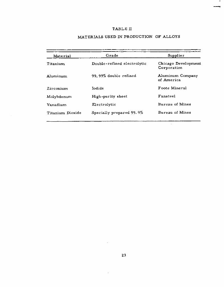
TABLE II
MATERIALS USED IN PRODUCTION OF ALLOYS
Material Grade Supplier
Titanium Double-refined electrolytic Chicago DevelopmentCorporation
Aluminum 99. 997o double refined Aluminum Company
of America
Zirconium Iodide Foote Mineral
Molybdenum High-purity sheet Fansteel
Vanadium Electrolytic Bureau of Mines
Titanium Dioxide Specially prepared 99. 9% Bureau of Mines
?3
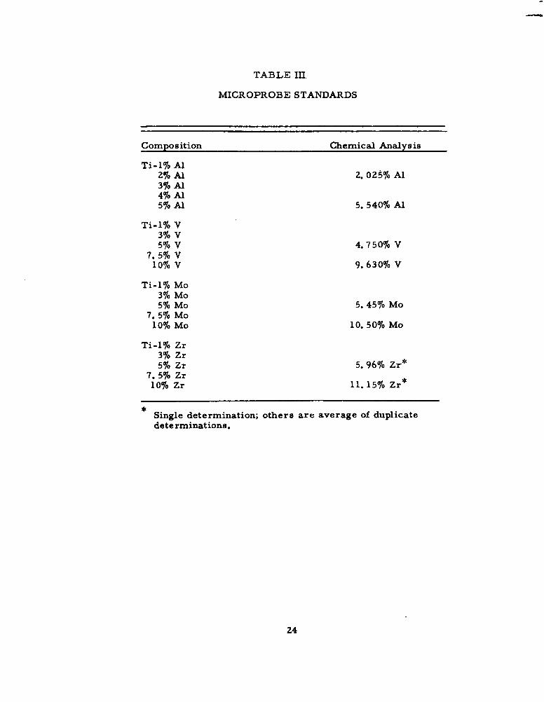
TABLE III
MICROPROBE STANDARDS
Composition Chemical Analysis
Ti-l% Al2% Al 2. 025% Al3% Al4% Al5% Al 5. 540% Al
Ti-l% V3% V5% V 4.750% V
7.5% V10% V 9.630% V
Ti-l% Mo3% Mo5% Mo 5.45% Mo
7.5% Mo10% Mo 10. 50% Mo
Ti-l% Zr3% Zr5% Zr 5.96% Zr*
7.5% Zr10% Zr 11. 15% Zr*
Single determination; others are average of duplicatedeterminations.
24
o Lf0 P4 14 P" I -4I
-4
En a 0
0 E-4
o co
N N0 0 0 a 00 0 0f0 ~ ~ ~ ' a, C, NN N N
0. eq. I C)
o c 00c o 10 0
o ~ ~ 0o o'a N Nz u'£ a4)P4
rz.I
I-
0 0
U N n" u > Ln L r n -4
a > .. a a a ".
N- H -H E r-4H H H
25
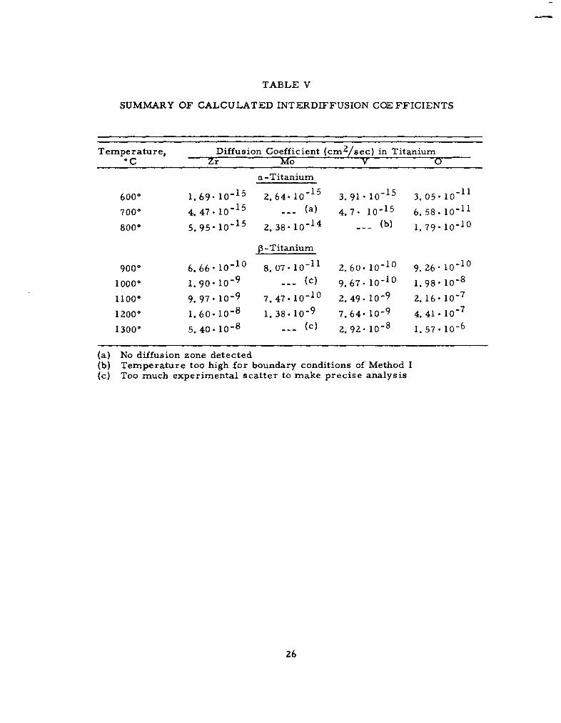
TABLE V
SUMMARY OF CALCULATED INTERDIFFUSION COEFFICIENTS
Temperature, Diffusion Coefficient (cm 2 /sec) in Titanium0C Zr Mo V 0
a-Titanium
6000 1.69.10-15 2.64. 10"15 3.91•10-15 3.05 •10-11
700° 4.47.10-15 --- (a) 4.7. 10"15 6.58.10-11
800* 5.95"10"15 2.38"10-14 --- (b) 1.79.10-10
P- Titanium
9000 6.66"10-10 8.07.10-11 Z.60.10-10 9.26"10-10
10000 1.90"10-9 --- (W) 9.67 I0-10 1.98" 108
11000 9.97" 10-9 7.47.10-10 2.49. 10-9 2.16"10-712000 1. 60 .10-8 1. 38 .10-9 7.64- 10-9 4. 41-•10- 7
13000 5.40.10-8 --- (c) 2.92"10-8 1.57.10-6
(a) No diffusion zone detected(b) Temperature too high for boundary conditions of Method I(c) Too much experimental scatter to make precise analysis
26
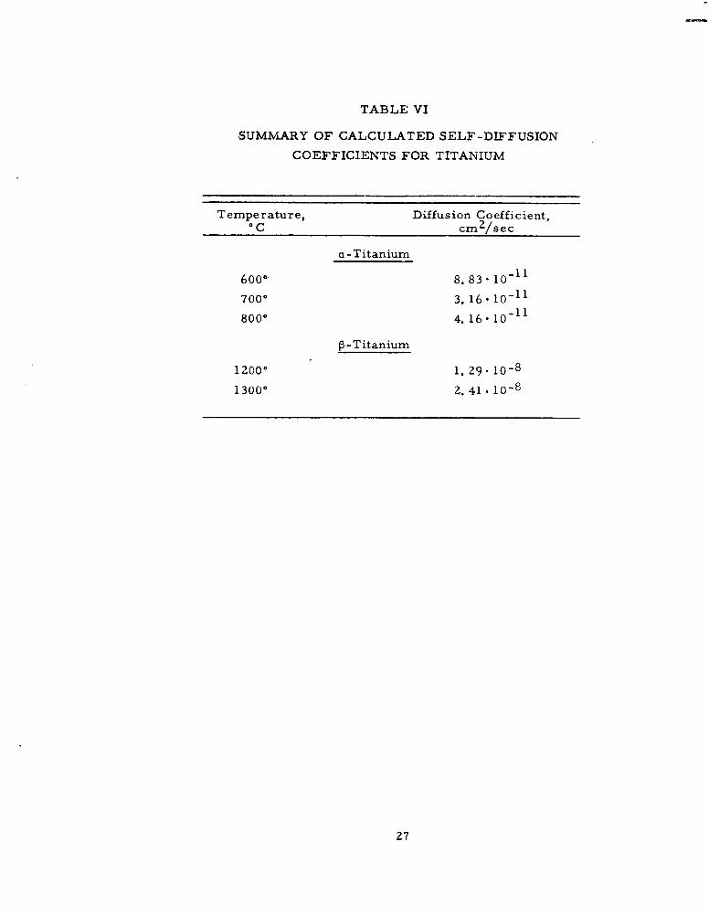
TABLE VI
SUMMARY OF CALCULATED SELF-DIFFUSION
COEFFICIENTS FOR TITANIUM
Temperature, Diffusion Coefficient,°C cm 2 /sec
a- Titanium
6000 8.83 " 1 1
7000 3.16"10-11
8000 4. 16 "10-1
P-Titanium
12000 1. 29. 10-8
13000 2. 41 • 10-p
27
2 PHASE PUREALLOY SOLVENT
tw=
Solubility Limit0(n > t2>tj >to Sto ý
tj 2
X -- 0 - X +
METHOD I
SOLID SOLUTION PURE
Concentrotion of Solute SOLVENTinitiolly Ci
to
2 ti t2>tI > to
C/C* 0.5
0-XE- 0 -. X +
METHOD IT
FIG. 1 - SCHEMATIC DRAWINGS SHOWING DIFFUSIONFOR SUCCESSIVE TIMES IN METHODS I AND II
Z8
w -i
LL.)
oc(n
Iw
U -
0~
-I-
CL&
0~
Ui U-
Z )z z
0
I-rn -
0 ) 0 U
.4bW
w 0
29
A 3
0.062 ±.005 047±053
FIG. 3 - TITANIUM SPECIMEN FOR SELF-DIFFUSION STUDIES
30
zz
ww
X I.)-
IA 0
zw 0
IA 2
aw 0z AJ - W u a.L
0 -0
L U) -
hi 9-
2 w
00
U
UU
a. u0-
31
210
zoo o0 10
0
190
o00U--
S180-a4
o. U ~4.
* 170-
2c-o .
S160-o
0
U I Solubility Limit -- 3.3o IU 0
140
130-
040
-___j0
0 0 02 0I I I I I I
0 2 4 6 8 10 12 14 16 18 20 22 24 Z6 28
Penetration, cm- 104
FIG. 5 - PENETRATION CURVE OF Ti/Ti-10V COUPLEANNEALED 720 HOURS AT 6000C.
32
____ ____ ____ ____ ___ ____ ____ ____ __
%0
0 N
'0
0N
00
00
0
N
o, H00
0 ~ N
10 Nnf
pUODas/s;uflo aIlnTp'eueA uOVBI.Ku93uOD
33
00
zo z
0 0
0
U
0
Lf) P
U 00
0
00
o-
1f
WO -TDc 3010A 'UORAXNJ uoTI-ellugOUtz
34
0, 98
6000 7000 8000
0. 95
0.90
0
0 0 0.80u U
u u 0.70
0f 0.60-.o
S0.500
0.400
u 0.30
0 0 20"U 0
S0.10C
0 05
0,02 I I p
0 5 10 15 20 25 30 35
Relative Penetration, cm. 104
FIG. 8 a - PROBABILITY PLOTS OF Ti/Ti-5Zr COUPLESANNEALED AT 6000, 7000, AND 800°C FOR"7•2 0 IOURS.
35
0.98
9000 10 00 11000 12000 13000
0.95- 00
. 00.90 0
0S00
'j 0.804
e, 0.70-0
0.60 0
0 o/0.505
0u 0.402-4
o0.30u
$4, 0.20-
0.10 -0
0.05-/
0. 02 I
0 10 20 30 40 50 60 70 80
Relative Penetration, cm. 102
FIG. 8b - PROBABILITY PLOTS OF Ti/Ti-S Zr COUPLES ANNEALEDAT 900% 1000%, 1200% AND 1300-C FOR 520, 140, 44, 16,AND 4.4 IHOURS, RESPECTIVELY.
36
0. 98
0.95-
0.90-
N 600' C 8000C9F 0.70 -
S0.60-0
E 0.50-
u) 0.40-
0 0. 30-
u S0. 20-
0. 10-
0.05 - , iI
0 2 4 6 8 10 12 14Relative Penetration, cm .10 4
FIG 9a -PROBABILITY PLOTS OF Ti/Ti-TMo COUPLESANNEALED AT 6000 AND 800°C FOR 7Z0 HlOURS.
37
0. 98
9000 11000 12000
0. 95
0.90
0 0
0.80-00
- 20.70
o lu 0.60 -. 0
00. 50
0 0.40
0 0.30
S0. 200
S0. 10
0.05
0.02 I I L0 5 10 15 20 25 30 35
Relative Penetration, cm. 102
FIG. 9b - PROBABILITY PLOTS OF Ti/Ti-5Mo COUPLESANNEALED AT 900", 1100°, AND 1200I C FORFOR 420, 92, AND 48 HOURS, RESPECTIVELY.
38
0.98
0.95
0.90
0.80
0 00o.7 -o 600060001H0. 0 7000
" 0.500I 0.400
0. 300
0 . 20
u 0. 10
0. 05
0. 02 I I
0 2 4 6 8 10 12 14
Relative Penetration, cm. 104
FIG. l0a - PROBABILITY PLOTS OF Ti/Ti-10V COUPLESANNEALED AT 6000 AND 7000C FOR 720 HOURS.
39
0.98 9000 10000 11000 12000 13000
0 0
0.95-0
0.90
0.800
0 0 0.70-
ulu 0.60
o 0.50
® 0.40 001.4
S0.300
0 0S0.10-
0. 05 /0 0 0
0.02 1 i I i i I
0 10 20 30 40 50 60 70 80
Relative Penetration, cm. 102
FIG. 10b - PROBABILITY PLOTS OF Ti/Ti-SV COUPLES ANNEALEDAT 900, 1000%, 1100%, 1200, AND 1300°C FOR 520, 140,44, 16, AND 4.4 HOURS, RESPECTIVELY.
40
0.98
6000 7000 8000
0.95
0.90o
0. 80
0 0 0.70-
4 0.60
e 0 5004j 0.400O 0.300u) 0. 20
00
u 0. 10
S0.05
0
0.02 10 5 10 15 20 25 30 35
Relative Penetration, cm. 10 2
FIG. lla - PROBABILITY PLOTS OF Ti/Ti-0.50 COUPLESANNEALED AT 6000, 700°, AND 8000C FOR1000 HOURS.
41
0. 98
900° 10000 11000 12000 130000.95- 0
0 0
0.690
0.800
0 o0. 70-0 00 0S0.60- 0
004 0
4.00
O. 021JtIt
0 20 40 60 80 100 120 140 160 180
Relative Penetration, cm. 102
FIG. lib - PRO'3ABILITY PLOTS OF Ti/Ti-0. 50 COUPLES ANNEALED AT900-, 1000°, 11000, 1200, AND 1300-C FOR 900, 135, 48, 14,AND 4. 8 HOURS, RESPECTIVELY.
42
Temperature, 6C 600700
100,000 800
10, 000
-4 1,000A Ti/Ti-5Zr
C) Ti/Ti-1yV
10 Ti/Ti-7Moqý 10 0
0U
002,4.4
1.
0. 1• ""'---
0.92 0.96 1.00 1.04 1. 08 1.14 1. 16
1000Temperature, -r-
FIG. 12 - SUM!MARY OF DIFFUSION COEFFICIENTS FOR ZIRCONIUM,
MOLYBDENUM, VANADIUM, AND OXYGEN IN a.TITANIUM.
43
Temperature, "C1300 1200 1100 1000 900
100, 000 , I I ,
10, 000
o 1,0000
u 100
L)
0
0 . 010
1. 0 iT -Z0
0 Ti/Ti-5V
o Ti/Ti-5Mo
0.1 I0.65 0,70 0.75 0.80 0.85
1000Temperature, 1000
FIG. 13 - SUMMARY OF DIFFUSION COEFFICIENTS FORZIRCONIUM, MOLYBDENUM, VANADIUM, ANDOXYGEN IN A-TITANIUM.
44
Ti44("1OO r) 0+
ElectronCapture
144 key I +
68 or 76 key 2+
0_ 3+
Sc44 (3. 92 hrs)
and Electron Capture
(Energy p+ = 1. 471 Mev)
2. 54 Me 9. 9%
1. 159 Mev 2+
0 0+
Ca 4 4 (Stable)
FIG. 14 - DECAY SCHEME OF Ti 4 4
45
(Penetration, cm. 102) 2
10005 10 15 20 25 30 35_III I !
d1000
o00
0
10044.
0)0
0
0 1 2 3 4 5 6
(Penetration, in. 102 ) 2
FIG. 15 a -PENETRATION CURVE OF SELF-DIFFUSION COUPLEANNEALED AT 6000 C FOR 60 DAYS.
46
(Penetration, cm. 102) 2
10005 10 20 5 30 35
001000 ,
-0
o0o 0
0 0u 00
00"-4
'.0
0
0
0 1 2 3 4 56
(Penetration, in. I0)Z
FIG. 15 b -PENETRATION CURVE OF SELF-DIFFUSION COUPLEANNEALED AT 7000 C FOR 60 DAYS.
47
(Penetration, cm. 102)2
10 ipz 0 z5 30 351000 T
0
00
S100 0
0u
0 -
"-4-
00• 1
1 • I I I
0 1 2 3 4 5 6
(Penetration, in. 102) 2
FIG. 15 c - PENETRATION CURVE OF SELF-DIFFUSION COUPLEANNEALED AT 8000 C FOR 60 DAYS
48
(PeneLratioi, cm-. 102))2
1000 10 20 30 40 50 60 70IuuI , I
r- T
Ln0 -
100-0
u
1 I a-
o0 l
0 1 2 3 4 5 6 7 8 9 10 11 12
(Penetration, in. 102)2
FIG. 15 d - PENETRATION CURVE OF SELF-DIFFUSION COUPLEANNEALED AT 900 C FOR 60 DAYS.
49
(Penetration, cm. 102) 2
10 20 30 40 50 60 701000_
0
S100
0 5
4.,
4-,
u 10 -0
1 I I I I I I I I l I
0 l 2 3 4 5 6 7 8 9 10 1l 12
(Penetration, in. 10l2) 2
FIG. 15 e - PENETRATION CURVE OF SELF-DIFFUSION COUPLEANNEALED AT 10000 C FOR 30 DAYS.
50
(Penetration, cm- 10z)z
1000 10 20 30 40 50 60 70
100
0
" 0
u
o 0
""-4
~ 10
1, I I I I I I I I J
0 1 z 3 4 5 6 7 8 9 10 11 lz
(Penetration, in, .102) 2
FIG. 15 f - PENETRATION CURVE OF SELF -DIFFUSION COUPLEANNEALED AT 1200° C FOR 24 HOURS.
51
(Penetration, cm. 102) 2
1000 10 20 30 40 50 60 70
1000
00
0
.4*m 100
0
0 10
00
0 1 2 3 4 5 6 7 8 9 10 11I1(Penetration, in. 10107)
FIG. 15 g 3PENETRATION CURVE OF SELF-DIFFUSION COUPLE
ANNEALED AT 1300"C FOR 3 HOURS.
52
Temperature, OC
I z0o130C 1100 1000 900 800 700 600
S I - I I I I i
1,000
100-0
U 100-
0
0.6 0. 7 0.8 o.9 1.0 1. 1 1. 2
Temperature, 10002TOK
FIG. 16 - SUMMkARY OF SEL:F-DTFFTJSTON COEFFICIENTSFOR TITANIUM.
53
APPENDIX I
THE PRODUCTION OF RADIOACTIVE Ti 4 4
By bombarding scandium with 22 Mev &rotons, radioactive Ti 4 4 wasmade by the nuclear reaction Sc 4 5 (p, 2n) Ti4 . The scandium metal wascontained on an aluminum target.
The following procedure was developed by the Nuclear Science andEngineering Corporation to separate Ti 4 4 from the scandium. Prior tobeing used with the bombarded sample, the chemical procedure was testedand shown to yield in excess of 90% of the Ti 4 4 .
Several unsuccessful efforts were made, including those based onthree solvent extraction methods, on the NH 4 OH-H 2 0Z precipitation method,
and on other precipitation methods. The successful procedure is givenbelow.
Procedure:
The scandium was etched from its aluminum backing with HCL.Appreciable amounts of aluminum were also dissolved. After saturating thesolution with HCl gas, at ice temperature, the AICl 3 precipitate was centri-fuged off. This precipitat~e was washed with HCl several times, and allliquid phases combined.
The active solution was passed through a Dowex-l anion exchangecolumn which had been conditioned with 12 N HC1. Under these conditions,The Ti 4 4 was found to be tightly bound to th-e resin, while the aluminum andscandium remaining in the active solution were eluted readily by washingwith 12 N HC1. Ti44 was finally eluted with 9 N HCl, and the volume reducedby cautious evaporation.
The Ti44 was coprecipitated on Fe(OH).3 . The precipitate wasdissolved in 12 N HCI, and the resin purification repeated. The final eluatewas evaporatedto near-dryness and diluted to desired volume. Ten milli-grams of titanium were added, and NH 4 OH was added to form the hydroxide.This was filtered off and ignited at 8000 C for 30 minutes to focm the TiO2product.
An energy spectrum of the product received from Nuclear Scienceand Engineering Corporation was determined at Armour Research Foundationon a 512 channel pulse height analyzer. Only activities of Ti 4 4 and Sc 4 4
(a daughter of Ti 4 4 in the decay scheme) were observed. Thus, the purityof the product was substantiated. The yield was confirmed to be -15 micro-curies as had been stated by Nuclear Science and Engineering Corporation.
54
APPENDIX- II
SAMPLE CALCULATIONS OF DIFFUSION COEFFICIENTS
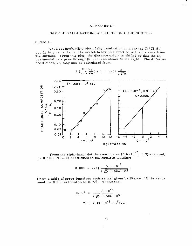
Method II:
A typical probability plot of the penetration data for the Ti/Ti-5Vcouple is given at left in the sketch below as a function of the distance fromthe surface. From this plot, the distance origin is shifted so that the ex-
perimental data pass through (0, 0.50) as shown on the ri.ht. The diffusioncoefficient, D, may now be calculated from
2 ( 2 I = erf(c 1 -co 2 TD-
0.98t 1.584 105 sec.z 0.95-
00.90 -0 3.6 10-2, 0.9)--.
0) C:0.9060-
2• 0.700 0
0< 03 oz 0.30 -0
0.10 - 0
0.05 -0
0.02 I I I I0 2 4 6 8 10 12 -6 -4 -2 0 2 4 6
Cm . 10 2 Cm • I0 2
PENETRATION
From the right-hand plot the coordinates (3.6. 10-, 0.9) are read;c = 0.406. This is substituted in the equation yielding:
3.6 •10 20
0.800 = erf (2 VD • 1. 584 .10 5
From a table of error functions such as that given by Pierce ,33) the argu-ment for 0. 800 is found to be 0. 906. Therefore:
0. 906 = - 3.6* lo-2 VD'.584 .10-9 I
D = 2.49 10-9 cmz /sec
55
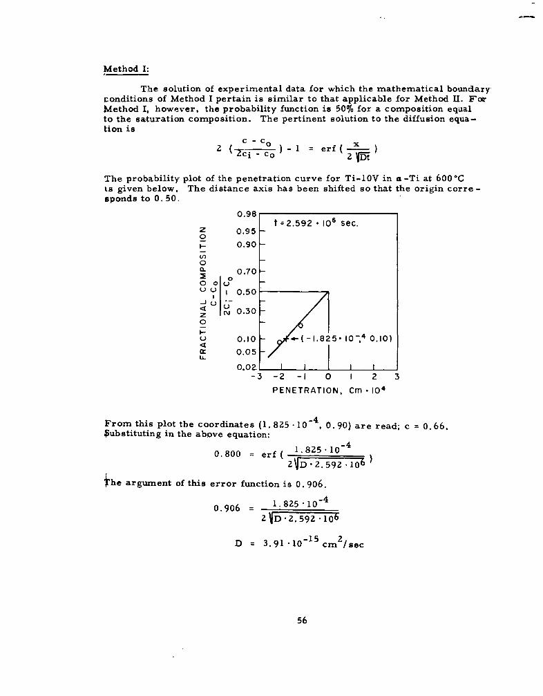
Method I:
The solution of experimental data for which the mathematical boundaryconditions of Method I pertain is similar to that applicable for Method TT. ForMethod I, however, the probability function is 50% for a composition equalto the saturation composition. The pertinent solution to the diffusion equa-tion is
2 c - co x- -ci_ o )" = e 2 ( Dt
The probability plot of the penetration curve for Ti-1OV in a -Ti at 600°Cts given below. The distance axis has been shifted so that the origin corre-sponds to 0.50.
0.98t 2.592 I06 sec.
z 0.95 -
0.90 -
0°0.70
2 0
(~OI0.50
0.02 I I
-3 -2 -I 0 I 2 3
PENETRATION, Cm- 104
From this plot the coordinates (1. 825 10-4, 0.90) are read; c = 0.66.Substituting in the above equation:
0.800 = erf ( 1.825102?JD • 2. 592 •106 )
ihe argument of this error function is 0. 906.
0.906 1.825 •10-4
2 D "2. 592 "106
D 3.91 "10-15 cm u/sec
56
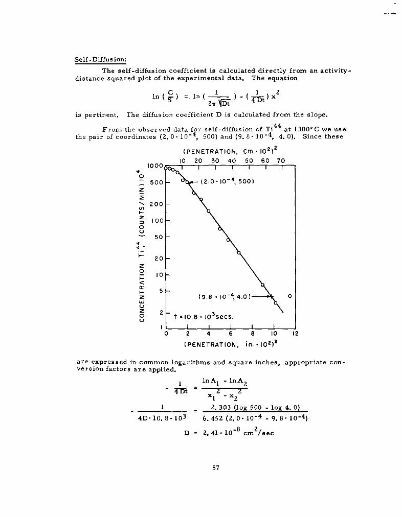
Self-Diffu s ion:
The self-diffusion coefficient is calculated directly from an activity-distance squared plot of the experimental data. The equation
in ( C in ( I I ) X2
is pertinent. The diffusion coefficient D is calculated from the slope.
From the observed data for self-diffusion of Ti44 at 13000C we usethe pair of coordinates (2.0- 10-4, 500) and (9.8. 10-4, 4. 0). Since these
(PENETRATION, Cm •02)2
10 20 30 40 50 60 701000
-500 -(2.0-10-4, 500)z
N- 200-U)i--
z=) 100-0
- 50
20z0- 10
I- 5z (9.8 10-44.0) 0LAJ
C-)z 230 t =10.8 . 10 3 secs.o
I I I I I I0 2 4 6 8 10 12
(PENETRATION, 'in.. 102)2
are expressed in common logarithms and square inches, appropriate con-version factors are applied.
1 In A 1 -lnA2z 2
1 _ 2. 303 (log 500 - log 4. 0)
4D'10.8. 10 3 6.45Z (2.0 10-4 - 9.8. 10- 4 )
D = 2,41 - 10"8 cm2/sec
57
~ % 0 6441
0 * 0
0 4-4N 0 Iý .0 0 .-
-4 (o' 0 $4.O .
'4+0';4 HO 0 V 0 000 0)>~
IJ 0 646 E40 IW .0 0, E4'- ~ -... 0 0 0 CD~ 0 ,'0 , 0
64 -OE .y6 -4 + 00 >41 0 .-464.0~ ~~ ~~ 0. 4 0 004O~c.
A~. 0.- *. ,0 0k o.6.4 00u 0' CD 0 a4 0 Vo0 ý4E0~- 01 0. . .4 '0 13> 1 1 C .4-
640 v 0 0 .44. -4... 4 .4
0 00 4- x 00 4.2 00 z0)' ).40 0000~
0 644
-.44. 9: 4- 0I 0+ M0 0 r 4 .H ..>00 01 "4 0 440 'S0'0 0 '4.- o
0 x4)- 4'06 0, M, q0 .04 0 >..
0 40Z 0 0
(a. 'U 0 7a w0 o4 0 0 0 4 0 ) 4 N -A 06
V 4-OR 1. m4.0 0 640 00,464 P.4 0 0 03 'om4 01 00.-4 'u4+ 0 n0.4X0 00 .. 40m
0 40 0 0'0 646 0w4 L000 .0 4. 1'''.0 0-.
0 4 ý: r )1 ! ,0' z- 14 0 ,wVr m . 4( ,
I.0 00 0 -OCPOP d oPk 10 ~ 0 0 44 )- 400ý:
6O-0. 0 4 0.
a 44
'4 ~ ~ ~ ~ ' 144 40 ~ ' '.
000
090. 0.- 0444 0f4 E4 C) 11- 0. m
I4. o 0~
%44004'U'0.4 .
00.40. A 4' ~ 4
A ~ jd :164. .4~ 00-00 0 ~ ' 00 00
04 0 .4 0. 0 0 0 03 A2 .4 a 404 .. 0. '4 04' 004 04 0.
~~0 4. "-'4 '4 t 0'
'D6 I . . j 0 0 0 6 ' 4. 0 0C; 40 ~ -. 100 00 40> 40 . 4 -P00A0.0.0
00 .40 .
-. 40 6440, 0 003i. 0 U>. .4 '0ý4I
A34 .000X t0
-1 p 00-4t4_00 1..~ .00-0 do; 02 :
PO U4 00 c:'a .0 44o 1. 0 14 0.0C3 644P
o 4- 'A '4.