“unconventional” monetary policy as conventional...

“Unconventional” Monetary Policy as Conventional Monetary Policy: A Perspective from the U.S. in the 1920s

Mark Carlson

Burcu Duygan-Bump*

PRELIMINARY DRAFT

August 9, 2017

To implement monetary policy in the 1920s, the Federal Reserve utilized administered interest rates and conducted open market operations in both government securities and private money market securities, sometimes in fairly considerable amounts. We show how the Fed was able to effectively use these tools to influence conditions in money markets, even those in which it was not an active participant. We also provide evidence that the changes in money market conditions resulting from changes in monetary policy affected the issuance of money market securities. These results point to a channel through which monetary policy was transmitted to the rest of the economy. The tools used in the 1920s by the Federal Reserve resemble the extraordinary monetary policy tools used by central banks recently and provide further evidence on their effectiveness even in ordinary times.

Key words: monetary policy, unconventional monetary policy, central banking, administered rates, money markets

JEL codes: E52, E58, N22

* Carlson: [email protected]. Duygan-Bump: [email protected]. We thank Jim Clouse, Barry Eichengreen, Bill English, Kenneth Garbade, Elizabeth Klee, Jonathan Rose, Judit Temesvary, David Wheelock and seminar participants at the Board of Governors and the NBER DAE Summer Institute for valuable comments. The views expressed in this paper are those of the authors and not necessarily those of the Board of Governors of the Federal Reserve or its staff.

- 1 -

In recent years, the Federal Reserve (Fed), like many other central banks, has introduced

new tools to implement monetary policy, including large scale asset purchases and use of

administered rates. Several of these tools were introduced as unconventional and temporary

policy tools, but some have argued that the Fed may have to rely on them more frequently going

forward. That might be the case, for example, if there has been a decline in the long-run neutral

real rate of interest—that is, the inflation-adjusted short-term interest rate consistent with

keeping output at its potential on average over time—as suggested by Clarida (2014) and

Holston, Laubach, and Williams (2016). Indeed, scholars and policy makers have increasingly

engaged in a broader debate about how central bank policy should be implemented, including

whether the central bank should use administered rates or target market rates and whether the

size and composition of the balance sheet should be used as policy tools (Stein 2012, Goodfriend

2014, Reis 2016, and Yellen 2016). An important part of the debate about which tools might be

part of the toolkit is whether these tools are effective and a growing literature has sought to

evaluate their effectiveness, particularly of the asset purchases (Krishnamurthy, Vissing-

Jorgensen, Gilchrist, and Philippon 2011; D’Amico, English, López-Salido, and Nelson 2012;

Altavilla, Carboni, and Motto 2015; and Haldane, Roberts-Sklar, Wieladek, and Young 2016).

However, such assessments are challenging given the limited number of actions and the fact that

several asset purchase programs were announced following the financial crisis when market

responsiveness may have been different than in normal times.

This paper provides a historical perspective on the tools available to the Fed by reviewing

the U.S. monetary policy toolkit and analyzing the transmission of monetary policy to private

money markets in the 1920s. The tools using during this period are perhaps surprisingly similar

to the tools introduced recently and understanding their effectiveness as conventional policy

tools during the 1920s provides additional information on the potential effectiveness of such

tools today. In particular, the Fed implemented policy by adjusting administered interest rates

and by purchasing both private and government securities. While the asset purchases of

Treasuries used by the Fed in the 1920s were of a smaller scale than the recent ones, the

operations during two easing cycles in the earlier period did more than triple the Fed’s Treasury

portfolio. Similarly, the administered rates the Fed used then and in the modern period have

useful parallels in relation to the balance sheets of commercial banks, with rates affecting the rate

of return to holding a highly liquid asset and the banks’ cost of short-term funding.

- 2 -

In addition to the literature on how central bank balance sheets can be used to implement

monetary policy described above, our work also adds to the literature on understanding the

channels through which monetary policy is transmitted to financial markets.1 Traditionally, most

work on monetary policy transmission in the 1920s has focused on the reserves channel—that is

how the Fed’s actions affected the supply and cost of reserves. Our analysis adds to this body of

work by testing the reserves channel, but we also investigate whether other channels that have

been of interest in modern times, such as the portfolio balancing channel, have mattered as well.

Our analysis starts with a review of the tools available to the Fed in the 1920s to

implement monetary policy and a discussion of how they functioned.2 The monetary policy

toolkit at this time is particularly interesting because the Fed had three policy instruments at its

disposal, each of which worked in a slightly different fashion. The first tool was the rate the Fed

charged for discount window loans (or rediscounts) where banks could choose to borrow from

the Fed to obtain reserves. The second tool was the rate at which the Fed would purchase

bankers’ acceptances; this tool directly impacted the value of a particular money market

instrument and affected the cost (and incentive) for banks to obtain reserves by selling the

acceptances to the Fed. The third tool was open market operations in government securities in

which the Fed would add or subtract reserves through the purchase or sale of Treasury securities

at the going market rate.

After describing the three policy instruments and how they worked, we examine their

effectiveness in influencing conditions in money markets during the 1920s. The connection

between changes in the policy tools and changes in conditions in private money markets is a key

link in the transmission of monetary policy. We focus on the years from 1923 until 1929—after

distortions from war finance needs had diminished and before the onset of the financial distress

of the Great Depression. In particular, we test whether private money market rates in New York

City, where the major money markets in the U.S. were located, responded to changes in the

discount window rate of the Federal Reserve Bank of New York (New York Fed), changes in the

1 See, for instance, Hamilton 1997; Demiralp, Preslopsky, and Whitesell 2006; Carpenter, Demiralp, and Senyuz 2016; Duffie and Krishnamurthy 2016. 2 As we discuss in more detail below, we use the term monetary policy to refer to actions taken by the Fed and the consequences of those action. We touch only lightly on the intent behind such actions.

- 3 -

discount at which the New York Fed purchased acceptances, and changes in the System’s

holding of government bonds.

We find that the policy instruments were effective in influencing private money market

rates in the ways expected, higher administrative rates tended to raise private interest rates while

purchases of Treasury securities reduced private interest rates. Indeed, we find that the impact of

large-scale asset purchases on money markets was fairly substantial and had effects at least as

large, if not larger, than those that have been found for the recent asset purchase programs.3

Such results are in line with those of Bordo and Sinha (2016).

To gain more insight into the channels through which monetary policy was operating, and

particularly whether there were channels operating in addition to the reserves channel, we focus

on the bankers’ acceptance market and the Fed’s rate for purchasing these instruments. We test

whether the bankers’ acceptance market was sufficiently developed such that it enabled the Fed

to use changes in its acceptance rate to influence conditions in money markets through channels

in addition to the reserves channel. Certainly changes in the rate at which the Fed purchased

these securities affected the incentives of banks to sell the acceptances to the Fed and thus the

availability of bank reserves and financial conditions. However, it is possible that there were

additional effects. In the 1920s, the Fed supported the growth of the acceptance market (bankers’

acceptances were a money market instrument that could be used to finance trade) with the intent

that banks and other financial institutions use these instruments as part of their liquid

investments. To the extent that other institutions priced other instruments relative to

acceptances, then arbitrage may have meant that changes in the rate at which the Fed bought

these securities had sizable impacts on the prices of other money market securities.

Alternatively, the Fed’s support for the acceptance market resulted in the Fed buying over 40

percent of outstanding instruments at times. With this degree of intervention, it is not clear that

the price of acceptances necessarily would have mattered for any other market prices.

We test the channels of transmission by looking at whether the changes in reserves

appears to account for most of the change in money market rates. While we find that the effect

of purchases of Treasury securities and bankers’ acceptances were of similar magnitudes,

3 These comparisons are subject to numerous caveats. One particular caveat especially worth noting is that recent asset purchase program may have influenced financial conditions through different channels than the ones in the 1920s.

- 4 -

consistent with the reserves channel, we also show that, for acceptances, the change in the rate at

which the Fed purchased these securities had much larger effects than could be explained by just

the reserves channel. Instead our evidence is consistent with the interest rate arbitrage and

portfolio balance channels being important transmission channels during the 1920s, as in Bordo

and Sinha (2016).

The paper is organized as follows. Section 2 describes the Fed’s monetary policy toolkit

and discusses the implications of the use of these tools for the Fed’s balance sheet. Section 3

examines the empirical evidence on immediate transmission: both the connection between the

administered rates and the composition of the balance sheet and the transmission of changes in

these tools to conditions in private money market rates. Section 4 describes the analysis linking

changes in monetary policy to the larger economy. Section 5 concludes.

Section 2. Monetary Policy Toolkit

In this section, we review the three main tools the Fed used to implement monetary

policy in the 1920s—the discount window, purchases of bankers’ acceptances, and open market

operations in government securities—and how they shaped the Fed’s balance sheet. We also

discuss several mechanisms through which changes in these tools may have been transmitted to

private money markets.

Note that in this paper, our focus is the Fed’s toolkit and how the monetary actions taken

by the Fed affected money market conditions. We are neither focused on the reasons for the

policy actions nor whether the policy makers had the correct intentions behind their actions.

Wheelock (1991), Friedman and Schwartz (1963), Meltzer (2003), and Wicker (1966) provide a

detailed review of the factors driving monetary policy in this period.

Nevertheless, it is worth remembering that the Fed in this period was generally operating

a countercyclical monetary policy with a stated goal of accommodating commerce and business,

without allowing speculative excesses to create instability. The Federal Reserve would tighten

policy when they viewed credit growth as excessive, and ease when industry and trade were in

need of support. Conditions in financial markets were viewed as signals about the demand and

supply of credit growth. As noted by Wheelock (1991), these signals require careful

- 5 -

interpretation; for instance, low money market rates could signal low loan demand as well as

excessive supply of reserves, but the appropriate monetary policy response differs depending on

the underlying reason. Wheelock also suggests that the Fed interpreted the signals correctly in

the 1920s given the correlation between monetary policy and industrial production in this period.

2.1 The discount window

In the 1920s, one of the primary tools for implementing policy was the discount window,

where the Fed could (re)discount paper for banks or provide advances (loans) against eligible

collateral. The rates that were charged for providing credit through the discount window could

be increased or decreased in order to affect credit conditions. 4

The operations of the discount window were overseen by the 12 Federal Reserve Banks,

and the rates that were charged at the window were set by these banks subject to approval by the

Federal Reserve Board. As interbank markets were not quite as integrated in this period as they

are today, the Federal Reserve Banks had some scope to set discount window rates that differed

across districts.5 As our analysis focuses on the money market rates in New York, we focus on

the discount window rate at the New York Fed.6

The rates that the New York Fed charged on its discount window loans were often fairly

close to, but below, the interest rates on private money market rates in New York. These were

markets in which banks were typically lenders. The discount window rate was often above the

rates that the money center banks in New York banks typically paid on their deposits, including

their interbank deposits. As described by the New York Clearing House Association (1920), the

4 We think of this tool as operating similarly to the modern interest rate paid on the overnight reverse repurchase facility (ONRRP rate). By changing the ONRRP rate, the Fed affects the rate that important money market lenders can earn on a safe asset. That increases the rate of return the demand on other funds they provide, including the rate that banks would have to pay to borrow from these lenders overnight. By raising the discount window rate in the 1920s, the Fed was directly impacting the short-term funding rate that banks had to pay to borrow from the Fed. Note that the tools affect different sides of the Fed’s balance sheet: the modern tool affects the rate the Fed pays on one of its liabilities while the tool in the 1920s affects the rate the Fed earns on its asset purchases. 5 Efforts by banks to arbitrage differences in discount window rates promoted the early development of the federal funds market and the subsequent integration of interbank markets (Turner 1931). 6 The reserve banks could, and sometimes did, have multiple discount window rates that varied with the type of collateral being used. During World War I, all the reserve banks offered a preferential rate for loans backed by government securities in order to bolster demand for such securities. By the early 1920s, the New York Fed had a single discount window rate.

- 6 -

maximum rates that member banks were allowed to pay on interbank deposits and certificates of

deposit issued to banks in the early 1920s, were both below, and a function of, the discount rate

of the New York Fed.7 While the strict relationship between rates and the New York Fed’s

discount window rate was relaxed in the mid-1920s, it appears that the rates the money center

banks paid on many of their deposits remained below the discount window rate. The relative

expensiveness of the discount window is consistent with Burgess’s report that the New York

banks would often repay their discount window loans quickly when they received additional

funds due to gold flows or Fed asset purchases (Burgess 1936, p. 235-236).

During the 1920s, the ability of the Fed to provide credit through the discount window

was more limited than it is currently (Bordo and Wheelock 2013). In particular, the Fed could

only rediscount short-term commercial, agricultural, or industrial paper from member banks that

was used to produce, purchase, carry, or market goods. It could not discount promissory notes,

such as corporate bonds or longer-maturity commercial and industrial loans.8 The Fed could

also rediscount government paper. The amount the Fed provided a borrowing bank was less than

the promised payment at maturity by the discount rate. 9 In addition to discounting private paper,

the Fed could also make loans (advances) to banks for up to 15 days backed by either paper

eligible for discount or by U.S. government obligations. In general, during the 1920s, advances

tended to be secured by government securities while rediscounts tended to be of private paper.

Even with the restrictions on the paper it could discount or make advances upon, many

member banks accessed the discount window and the rate that the Fed charged on its rediscounts

and advances had an important effect on banks’ marginal cost of funding. Borrowing was fairly

widespread with about one-third of all member banks borrowing in any given month (roughly

3,000 borrowers out of 9,000 member banks). It is uncertain how much stigma was associated

with borrowing from the discount window in this period; even though we observe large numbers

7 Specifically, the rules stated that the maximum rate that member banks could pay on such deposits was set at one percent when the 90-day discount rate for commercial paper at the New York Fed was two percent. For each half-percentage point increase in the discount rate above two percent, the maximum rate that member banks could pay was increased by one-quarter of a percentage point (New York Clearing House Association, 1920, page 16). 8 Short-term was 90 days for commercial and industrial paper and 9 months for agricultural paper. Such restrictions grew out of the idea that the Federal Reserve should finance “Real Bills”. Temporary expansions of the Federal Reserve’s ability to lend against a broader range of collateral were made in 1932 and made permanent in 1935. 9 For details of this transaction see Hackley (1961). When discounting paper or receiving an advance, the bank incurred a liability to the Federal Reserve which would increase the bank’s leverage. Thus, these transactions had indirect costs to banks that open market operations in either acceptances or government securities did not.

- 7 -

of banks borrowing, contemporaries note that banks were reluctant to borrow, especially in the

money centers (Reifler 1930, p. 29-30).

2.2 Open market purchases of bankers’ acceptances

The Fed could purchase bankers’ acceptances in the open market as part of its open

market authority (while the Fed could purchase a slightly broader set of securities than just

bankers’ acceptances, acceptances constituted nearly all the paper bought by the Fed so we use

the term bankers’ acceptances to refer to all such paper).10 The primary use of bankers’

acceptances in the 1920s was as a money market instrument to finance trade, especially

international trade (Beckhart 1932). When an exporter shipped goods abroad, they typically had

to wait to be paid until the goods reached the market and were sold. Especially in international

trade, this could have taken some time. Rather than wait, the exporter could have brought a bill

indicating the shipment to his bank and received a loan against that bill. Bank financed such

loans by endorsing the bills and bringing them to larger banks, usually in a money center. The

money center banks would then “accept” the bill and provide money to the exporter’s bank. The

money center bank could hold that bill and finance it as it would any other security it held or the

bank could sell the bill into the market as a bankers’ acceptance. The acceptance was guaranteed

by the payment the exporter expects to receive, the promise of the exporter’s bank to make good

on the paper if the exporter failed, and the promise of the money center bank to make good on

the paper if the exporter’s bank failed. Triply secured, the bankers’ acceptance was low risk and

short term, perfect as an instrument for money market investors.11

This type of instrument was little used in the United States prior to the Federal Reserve.

Indeed, banks with National charters were forbidden to issue such securities. As many

prominent European money markets, such as London, had large bankers’ acceptance markets and

the fact that these securities backed “real transactions,” the founders of the Federal Reserve were

10 The Federal Reserve still has the authority to purchases bankers’ acceptances, however, it has not used this authority in some time. Open markets operations in bankers’ acceptances and the use of repurchase agreements on bankers’ acceptances to manage reserves were ceased in 1977 and 1984, respectively. See Small and Clouse (2005). 11 It is not clear what the maturity structure of these instruments at origination was, but at particular points in time, roughly 40 percent of the holdings of the Fed had maturities of less than 15 days, 20 percent had a remaining maturity of between 16 and 30 days, 25 percent had a remaining maturity of 31 to 60 days. The rest had a maturity of more than 60 days.

- 8 -

keen to develop this market in the U.S., which would also help promote the U.S. dollar as an

international currency (Ferderer 2003, Eichengreen and Flandreau 2012).

The Fed had a passive role in the open market operations in bankers’ acceptances.

Instead of directly buying a certain amount of acceptances directly from the market, the Federal

Reserve banks would set the rates at which they would buy acceptances of particular maturities,

where this rate was the discount relative to the face value of the acceptance; we refer to this

discount as the acceptance rate. The Fed would then take all eligible acceptances that were

delivered to them.12 Given the desire of the Fed to promote this market, the rate at which the

Fed would buy acceptances tended to be set favorably relative to the rate at the discount window.

Thus, the incentives of banks to issue acceptances and deliver them to the Fed were influenced

both by the level of the acceptance rate, but also by the spread between the acceptance rate and

the discount window rate.13 As with rates at the discount window, the 12 reserve banks could

each set their own rates for purchasing these securities. Moreover, each reserve bank would

often have multiple acceptance rates that depended on the remaining maturity of the acceptance.

Again, given our focus on the New York markets, we use the rates offered by the New York Fed.

The maturity of the acceptances that the Fed purchased were fairly short term. In a

typical month, around 40 percent of the acceptances that were purchased by the Fed had a

remaining maturity of 30 days or less. The Fed was willing to purchase acceptances with

remaining maturities of up to 180 days and the Fed’s modest purchases of these longer maturity

acceptances was sufficient to raise the average maturity of acceptances purchased by the Fed to

around 50 days. The Fed bought some of these acceptances outright, but also purchased

acceptances from dealers under agreements to resell at later date (repo agreements).

12 Eligibility rules covered issues such as the types of goods associated with the underlying transaction and the maturity of the loans being provided; interestingly, whether any of the banks involved in the transaction were Federal Reserve member banks did not affect eligibility. While all the reserve banks appear to have purchased acceptances, the largest acceptance markets were in Boston and New York. Purchases of acceptances by the Federal Reserve System appear to have been concentrated at the reserve banks in these cities and then apportioned to other reserve banks through a sharing agreement. 13 We think of this tool operating in some ways like the interest rate on excess reserves used currently by the Fed. When the Fed increases the interest rate paid on excess reserves, it increases the value of this asset and provides an incentive of banks to hold onto these reserves rather than lend them to another bank unless they are offered an even higher rate. Similarly, by changing the discount at which it purchased acceptances, the Fed could affect the value of these assets and the incentives of banks to hold them or deliver them to the Fed to obtain additional reserves. Note that, as with the previous tool, these tools affect different sides of the Fed’s balance sheet: the modern tool affects the rate the Fed pays on one of its liabilities while the tool in the 1920s affects the rate the Fed earns on its asset purchases.

- 9 -

2.3 Open market operations in government securities

The Federal Reserve also has the authority to purchase or sell government obligations in

the open market. Originally, each Federal Reserve Bank conducted open market operations in

government securities independently, which at times led to challenges that underscored the need

for better coordination. Efforts to coordinate operations across the System eventually resulted in

the creation of the Open Market Investment Committee in 1923.

Around this time, open market operations in government securities began to be seen as a

tool that could be used to manage the aggregate quantity of credit, and support the discount

window policy. Some shifts in policy were associated with large swings in the holdings of

government securities. For instance, in 1924, the Federal Reserve took steps to ease monetary

policy and increased its holdings of Treasury securities from $100 million in January to $600

million by October. In 1928, policy was tightened and holdings of Treasury securities fell from

$600 million in January to $200 million by June. At other times, changes in holdings of

government securities were modest; from January 1925 to July 1927 holding of government

securities average around $350 million, with week to week changes rarely exceeding $20

million. The Fed’s holdings of Treasury securities consisted largely of certificates of

indebtedness (with maturities of a year or less) and notes (with maturities of between one and ten

years). When the Fed engaged in substantial operations in Treasury securities, the more

substantial movements were in its holdings of notes (which would imply an extension of the

average maturity of its holdings) although at times there were also sizeable adjustments in the

Fed’s holdings of certificates.

With the Open Market Investment Committee, most purchases were conducted by the

New York Fed and allocated to the accounts of the other Reserve Banks. Purchases were not

announced, but were observable from the Fed’s weekly publication of its balance sheet. As with

acceptances, most securities were held out right, but some were bought under repo agreements.

During this period the Fed could purchase securities directly from the Treasury in some

circumstances. Such purchases were rare and were used for cash management purchases, but

when they occurred, they could be fairly large. See Garbade (2014) for details.

- 10 -

2.4 Balance sheet of the Federal Reserve

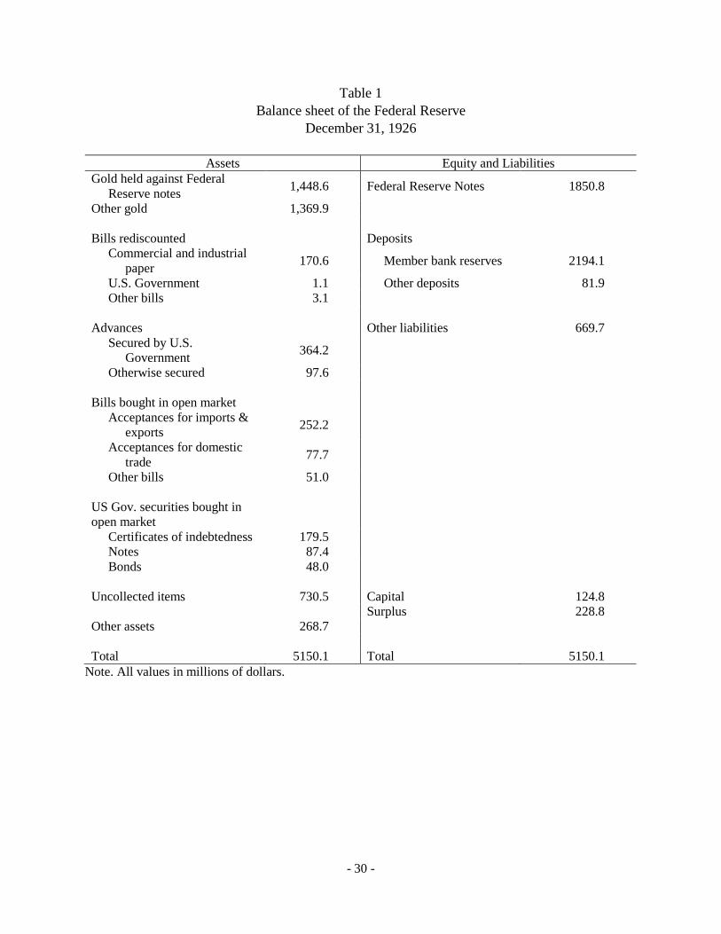
The balance sheet of the Federal Reserve for the year-end of 1926 is shown in Table 1.

From this table, it is clear that the major asset of the Federal Reserve System was gold, which is

consistent with the U.S. being on the gold standard.

It is also apparent that, during this period, the direct exposure of the Federal Reserve to

the condition of the commercial banking sector was fairly substantial. Private credit, consisting

of bills of acceptance purchased in the open market, paper rediscounted, or advances to member

banks on acceptable collateral (often government securities), constituted about 20 percent of the

Federal Reserve System’s assets. Advances, which were mostly secured by US government

securities, were typically more substantial than discounts, which were typically of commercial

and agricultural paper. Fed purchases of bankers’ acceptances securities represented seven

percent of the Fed’s assets. Most of the acceptances held by the Fed were associated with

imports or exports, though some were associated with domestic trade or inventory finance. The

Fed’s holdings of acceptances represented a significant share of the market, at times the Fed held

nearly 40 percent of outstanding acceptances. Consistent with its large share of the market, the

rate at which the Fed was willing to buy acceptances heavily influenced the market price. As

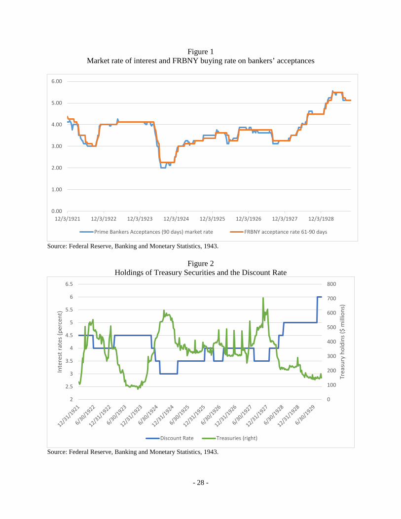
shown in Figure 1, the market rate in New York and the rate at which New York Fed offered to

purchase the securities were almost identical. Holdings of government securities were a smaller

share of the balance sheet in this period, averaging about seven percent of total assets.14

2.5 Channels by which money policy was transmitted to financial markets

In this section, we describe several channels through which monetary policy could have

been transmitted to financial markets. One of these, the reserves channel, was emphasized by

contemporaries. There are other channels however, many of which have been discussed recently

as central banks have employed a variety of tools to implement monetary policy.

14 At $315 million, the Fed’s holdings of Treasury securities represented about 1.7 percent of outstanding interest-bearing Treasury securities.

- 11 -

2.5.1 The reserves channel

The transmission channel described by contemporaries (especially Reifler 1930 and

Burgess 1936) is the reserves channel where the Fed affect the money market by changing the

supply and cost of obtaining reserves.15 Banks demanded reserves in order to comply with

reserve requirements and to facilitate their conduct of the business of banking; for instance,

reserves are useful for processing payment system transactions. The supply of reserves was

determined importantly by the Fed through its open markets operations. Purchases (or

sales/maturing) of Treasury securities would expand (contract) the supply of reserves. Open

markets operations in acceptances required that the banks decide to sell such securities to the

Fed, but the Fed could influence banks’ incentives by changing the discount at which it

purchased them. As these securities were short-term and naturally “self-liquidating,” they would

mature over time and tighten policy unless they were replaced. (Changes in monetary gold

should have had similar effects as open market operations and we typically include such changes

as a control variable. See Friedman and Schwartz (1963) for a discussion of the amount of gold

on the Fed’s balance sheet.) Banks could also obtain reserves by borrowing from the Fed

through the discount window. Changes in the rate charged on discount window loans would

have affected the willingness of banks to borrow from the Fed (supply of reserves) and the cost

of obtaining them (price of reserves).

Typically, the Fed would use its tools in a complimentary fashion during a shift in policy,

as seen in Figure 2 and discussed in (Burgess 1936). For instance, when tightening policy, it

would conduct open market sales of Treasury securities to decrease the supply of reserves. This

would make banks more reliant on obtaining reserves through the discount window. The Fed

could then increase the discount window rate to raise the cost of using the window. Moreover,

the Fed could also increase the discount on acceptance purchases so that banks received fewer

reserves when they sold reserves to the Fed which would further tighten the market for reserves.

As the reserves market tightened, these pressures would have been passed on to other money

markets.

15 This channel is also quite similar to discussions about the market for reserves and implementation of monetary policy in the late 1990s/early 2000s (see Koeger, McGowan, and Sarkar 2017).

- 12 -

While there was not yet a liquid market in which banks could directly trade reserves—the

federal funds market was still developing—banks could trade reserves indirectly through trading

securities and through their mutual participation in other overnight money markets and thereby

transmit monetary policy to these other markets. We illustrate this mechanism using an example

from the call loan market where brokerage firms obtained overnight funding (we describe this

market in more detail below). Suppose a bank is short on reserves. If that bank had lent funds in

the overnight call loan market, then that bank could acquire additional reserves by demanding

the repayment of its overnight loans from a broker. The broker would seek a new overnight loan

from a second bank that had sufficient reserves. By repaying the funds owed to the first bank

with funds from the second bank, the reserves would move from one bank to another. The

interest rate the broker had to pay the second bank was related to the scarcity of the reserves. If

reserves were plentiful, then there would be a larger number of banks ready to supply funds and

the rates in the call loan market would be lower. If reserves were scarce, then more brokers

would be competing for reserves from the fewer banks willing to provide loans and the call loan

rate would rise. Of course, the call loan market was not the only market in which banks could

indirectly trade for reserves. Other money markets in which short-term securities were traded,

such as the commercial paper market or even the bankers’ acceptance market, could fulfill this

role as could liquid markets in longer-term securities, such as Treasury securities. Because of

the variety of markets through which this transfer could occur and arbitrage across these markets

was not perfect, it would be hard to determine precisely how much a change in reserves might

change in monetary market rates, but the direction would be clear and would be consistent across

markets.

2.5.2 Interest rate arbitrage

The acceptance rate in particular may have been able to influence financial market

conditions in an additional, and more direct way. Certain investors held both acceptances and

other money market securities, such as commercial paper, as part of their portfolios. If the Fed

changed the rate at which it bought acceptances, and thus changed the prevailing market rate,

then we would expect the investors holding both assets to demand a different rate on other assets

in their portfolios. In this case, money market conditions should respond to changes in the

- 13 -

acceptance rate to a greater degree than would be expected just from the changes in the Fed’s

holdings of acceptances.

However, this mechanism depends on bankers’ acceptances being treated as an active

part of the portfolio. The Fed was heavily involved with this market and at times held more than

40 percent of outstanding acceptances on its balance sheet; the market price of acceptances

seldom differed from the rate at which the Fed was willing to purchase them. Given this

intervention, it is not certain that market participants would have used the rate on acceptances to

price other assets and the actions by the Fed may not have had any impact other than by

changing the supply of reserves.

2.5.3 Portfolio rebalancing

Another channel through which monetary policy might be transmitted to financial

markets is the portfolio balance channel (see discussion in Haldane, Roberts-Sklar, Wieladek,

and Young 2016). Underlying this mechanism is the idea that investors have preferences

regarding the assets they hold. If the central bank were to purchase a particular type of asset,

then the investors who had held that asset would purchase other assets with somewhat similar

characteristics in ways that would change the relative prices of these assets. For instance, if

certain investors have preferences for assets with a particular duration profile, then when the Fed

purchases large amount of longer-term Treasury securities those investors might purchase large

amounts long-term corporate debt and compress the yield spreads between these asset classes.

This compression in yield spreads might consequently promote issuance of corporate bonds. In

our period, the Fed was purchasing two types of assets – Treasury securities and bankers’

acceptances. Under the portfolio balance channel, we might expect that effect on money market

prices from purchases of bankers’ acceptances might be different, and possibly stronger, than the

effects from purchases of Treasury securities as the former are a more similar instrument.

2.5.4 Signaling/forward guidance

One last mechanism by which policy might be transmitted is through signaling; by

shaping expectations about whether monetary policy might be tighter or easier in the future, the

- 14 -

Fed would be able to affect the prices of assets that would mature after the change in policy was

expected to occur. Newspaper stories clearly indicate that market participants had expectations

about actions the Fed might take. Additionally, newspaper stories and analysis of changes in the

Fed’s balance sheet and in the discount and acceptance rates make it clear that financial market

participants were paying close attention to actions taken by the Fed. However it is not clear that

the actions taken by the Fed had strong impacts on reshaping the expectations of market

participants. To the extent that expectations were changed, it is more likely that the impacts

would be observable in long-term yields rather than in the very short-term interest rates

considered here. (Bordo and Sinha (2016) find evidence that shifts in market expectations

associated with changes in the Federal Reserve’s balance sheet mattered for longer-term

Treasury yields during 1932 when the Fed engaged in substantial purchases of Treasury

securities.)

Section 3. Impact of monetary policy tools on money market rates

In this section, we test whether changes in the monetary policy tools impacted rates in

money markets. As part of this first pass, we are agnostic about which channel the tools are

operating. Before testing the transmission, we briefly review the important money markets of

this period.

3.1 Review of major private money markets

There are two major private money markets that we use in our analysis. The first is the

market for broker’s loans, where short-term loans were extended to New York City stock brokers

and brokerage houses backed by equity securities traded on the New York Stock Exchange.16

This was the largest money market in the 1920s. Lenders included domestic and foreign banks,

corporations, and investment trusts. The domestic banks included both small banks across the

country and the major banks in New York.

16 There were smaller, less formal markets for providing funds to brokers on the regional stock exchanges or the New York “curb” market.

- 15 -

Loans were typically initially arranged at the money desk of the New York Stock

Exchange though some were also arranged through money brokers or directly between the large

banks and the brokerage houses. A large portion of the loans were demand loans and could be

called by the lender at any time which resulted in the market being referred to as the “call loan

market.” The market was seen as a place where liquid funds could be placed and was

sufficiently deep that, should a loan be called, the borrower was usually able to find another

lender and repay the first lender. Most call loans were rolled over from day to day with the non-

price terms of the loan being held constant. Further, there was sometimes a slight difference in

the interest rate for loans that were being rolled over (renewed) and new loans. Shifts in supply

and demand for funds had the most effect on the new call loans (as these would marginally add

or subtract to total loans made), and interest rates on these loans tended to be more volatile than

the interest rates on call loans that were rolled over. A modest share (30 percent) of loans to

brokers were made on a time basis. While not available at call, these loans were considered part

of the call loan market as they were to the same borrowers and secured by the same collateral.

There was also a portion of the call loan market where dealers could finance their

inventories of acceptances. This market does not appear to have been particularly deep and

seems to have virtually disappeared sometime in the early 1930s. Nevertheless, for the period in

which quoted rates appear, they track other rates in the call loan market reasonably closely which

suggests that this part of the market was fairly well integrated with the other parts.

The prime commercial paper market was a money market in which moderately sized

firms could borrow on an unsecured basis (larger firms would typically issue long-term bonds).17

The firms would issue short-term notes which would be purchased by a commercial paper house

which would arrange to distribute the paper around the country.18 The commercial paper houses

would verify the quality of the commercial paper they were buying and selling. While the

houses would not guarantee the paper they sold, there were reputational consequences to selling

17 To give a sense of size, in 1926 the average monthly outstanding volumes of the different money market instruments were Bankers’ acceptances: $691 million; commercial paper: $627 million, brokers’ loans on call $2,288 million, and brokers’ loans on time $825 million. There was an emerging federal funds market, but that was very small. There was also a repo market involving a variety of collateral, including bankers’ acceptances, but the size of this market is unknown. For additional details on these markets, see Beckhart (1932). 18 Distribution was facilitated by the tendency of these houses to be affiliates of a larger financial institution that engaged in other securities market activities, such as brokerage services or underwriting, and already had extensive relationships.

- 16 -

paper that subsequently went bad. The most common buyers of commercial paper were banks,

which would use this as a place to put funds on a short-term basis. Given the structure of the

market, while the borrower might refinance maturing commercial paper and the same

commercial paper house might buy and distribute that paper, the purchasers of one issue were

not commonly the purchasers of the refinancing issue. Banks might buy this paper directly or

through their correspondent, typically located in New York City. This market was fairly deep

for much of the 1920s, but started to fade by the end of that period.

Interest rates on this paper in the secondary market were determined by the quality of the

firm issuing the paper. “Prime” commercial paper reflected the paper considered by the National

Credit Office (a private firm affiliated with the R. G. Dun credit rating agency) to be of the

highest quality and the interest rates on that paper trading in the secondary market were used to

construct the prime commercial paper rate.

3.2 Setup of the analysis

To get a general sense of the relationship between the policy tools and market rates, we

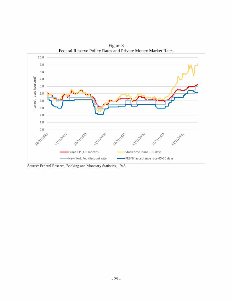
plot two policy rates and two private money market rates at a weekly frequency in Figure 3.19

The two policy rates are the New York Fed’s discount window rate and rate for purchases of

acceptances with a maturity of 16-30 days. The private rates are the interest rate on 90 day

commercial paper and the rate on time call loans (90 days).20 The figure suggests that, in

general, policy rates seem to have moved in the same direction though they were not adjusted at

exactly the same time. From Figure 2, we know that holdings of Treasury securities tended to

move inversely with these rates. Figure 3 also indicates that the private market rates moved

broadly at the same times as movements in the policy rates and the changes in holdings of

Treasury securities. It is also clear from Figure 3 that money market spreads during this time

19 As noted by Wheelock (1991), the Fed was reportedly attentive to whether its policy rates were out of alignment with market rates. Thus, there is some possibility of reverse causality in that changes in market rates could have caused the Fed to adjust its policies. However, it seems likely that any policy response would have been in reaction to more sustained changes in market rates rather than the week to week fluctuations analyzed here. Moreover, the results of Section [4.3] below using spreads between the money market rates and the discount rate should further alleviate concerns about reverse causality. 20 The private discount rate on acceptances is almost identical to the acceptance rate set by the Federal Reserve.

- 17 -

were positive and tended to move around over time, which is different than is the case now

where these spreads tend to be fairly tight and steady over time.

To more formally test whether private rates move in response to changes in policy

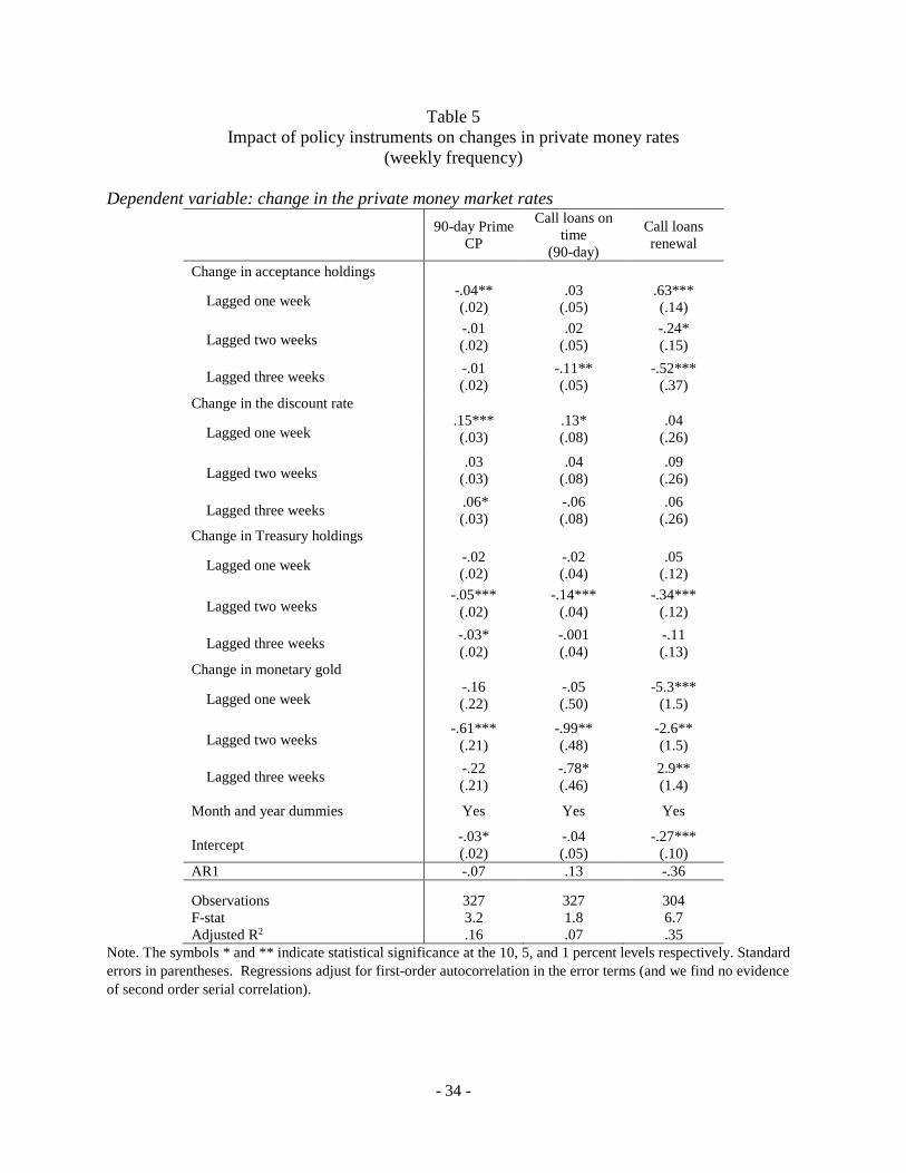
instruments, we regress changes in private money market rates on the changes in the policy tools.

(Using changes is a better test than using levels because of reduced likelihood of spurious

correlation and of issues associated with autocorrelation.) The private money market rates we

use are the interest rate on 90 day commercial paper, time call loans (90 days), and the interest

rate on (overnight) renewed call loans. The policy tools are: changes in the discount rate,

changes in the acceptance rate, and changes in the Fed’s holding of Treasury securities. The rate

at which the Fed discounted acceptances varied by remaining maturity of the acceptance; we use

the rate on acceptances with 30-45 days remaining maturity. For Treasury operations, we scale

the changes in the Fed’s holdings of to be in units of $100,000. Measuring changes in holdings

of Treasury securities in dollar units facilitates estimating the size of the impact of Treasury

purchases/sales; alternative scaling of the size of operations in Treasury securities produce

qualitatively similar results. As indicated above, increases in the administered rates should raise

private interest rates while increased holdings of Treasury securities should reduce them. We

include three lags of all the policy variables as this provides the best “fit.”

Changes in the Fed’s holdings of gold should also impact money rates in a manner

similar to Treasury purchases. (Hanes (2006) finds that gold flows affected monetary conditions

in the 1930s; gold inflows increased the supply of reserves and lowered longer term treasury

yields.) To control for the impact of gold on financial conditions, we include changes in the

monetary gold (measured in millions of dollars). Seasonal factors may also be important and we

include monthly dummies in the regressions. We also include year effects.

All variables are measured at a weekly frequency. Summary statistics for all variables

are included in Table 2. Our regressions control for first order serial correlation (although since

we are looking at changes at a weekly frequency, the effects of serial correlation seem fairly

minimal).

- 18 -

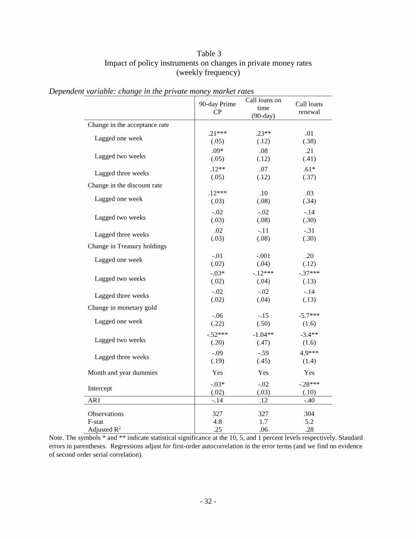
3.3 Results

The results are reported in Table 3. They are, for the most part, in line with our

expectations. We find that increases in both the acceptance rate and the discount window rate

raise private interest rates (with the exception that we do not find that increase in the discount

window rate raised the call loan rate). Increases in the acceptance rate appear to take some time

to fully effect the commercial paper rate. In general, private interest rates do not move one for

one with the policy rates; the exception is the call loan rate, which appears to move close to the

same amount as the acceptance rate.

Also as expected, increased holdings of Treasury securities are associated with reductions

in private money market rates. We estimate that an increase of $100 million in the Fed’s holding

of Treasury securities (an amount that would represent 2% of the balance sheet and was about

one-fifth of the actual increase in holdings in 1924) would have decreased the commercial paper

rate by 61 basis points. As the commercial paper rate averaged near 4 percent during this period,

the impact of Fed purchases could have had quite an impact on the rate.

We also compare this effect to the impact of purchases associated with the Fed’s large

scale asset purchases in the wake of the financial crisis. As money market interest rates were

already around zero when the Fed conducted its more recent purchases, we rely on estimates of

the shadow federal funds rate. Wu and Xia (2015) estimate that asset purchases of $100 billion

(which would also represent about 2% of the current Federal Reserve balance sheet) would be

roughly equivalent to the reduction in the federal funds rate of 10 basis points.21 Since

commercial paper rates tend to move almost one-for-one with the federal funds rate, one would

expect that $100 billion in purchases of Treasury securities would have a similarly sized impact

on this rate. Thus, our evidence suggests that Treasury purchases had large effects in the 1920s

than they do today. This results is similar to Bordo and Sinha (2016) who also find larger effects

of Treasury purchases in the 1930s than in modern times.

We also find that, again as expected, increases in monetary gold tended to reduce market

interest rates. We find modest seasonal effects, with interest rates tending to rise a bit more, on

average, during August, September, and October than other months. However the size of the

21 It should be noted that the estimate by Wu and Xia (2015) incorporates the effects from different channels than the one for the 1920s.

- 19 -

seasonal effects are small (4 to 5 basis points), consistent with the Fed having successfully

damped seasonal pressures (See Miron 1986, Carlson and Wheelock 2016).

Section 4. Some evidence regarding transmission channels

Our estimate of the relationship between changes in the monetary policy tools and

changes in the money rates was silent on which channels mattered. In this section, we provide

some evidence on which channels might have mattered. We focus on whether the monetary

policy tools might have mattered for reasons other than the impact on reserves. We focus in

particular on the how the role the rate at which the Fed purchased acceptances and the

acceptance market might have played.

4.1 Acceptances and the channel of transmission

The Fed strongly supported the market for acceptances. Part of this was to encourage

banks to include acceptances in their portfolio of liquid assets, in addition to commercial paper

and call loans. Part of the support was by acting as a buyer in the market (as noted above, the

Fed at times held over 40 percent of outstanding acceptances). If the Fed was successful in

convincing banks to hold acceptances in their portfolio of liquid assets (as was suggested by

Balabanis 1935), then changes in the acceptance rate ought to have caused institutions holding

acceptances to reprice other assets in their portfolio and changing the acceptance rate should lead

to larger effects than would be suggested just by the reserve channel. But, if the Fed distorted

that market by being such a significant purchaser of these instruments, then we would expect that

the reserve channel would account for nearly all the effect of this policy tool. To state this

argument slightly more formally, if the reserves channel accounts for the entire transmission of

the acceptance rate to market rates then estimated size of the effect on market rates from

changing acceptance rate directly:

Δ market rate = Δ accpt. rate + Δ discount rate + Δ Treasuries + Δ gold + other + ε (1)

- 20 -

should produce the same size effect as estimating the effect of the change in the acceptance rate

on changes in holdings of acceptances and the effect of the changes in holdings of acceptances

on changes in money market rates.22

Δ acceptances = Δ accpt. rate + Δ discount rate + Δ Treasuries + Δ gold + other + ε (2)

Δ market rate = Δ acceptances + Δ discount rate + Δ Treasuries + Δ gold + other + ε (3)

If there are other channels at work other than the reserve channel, then the effect estimated in (1)

should exceed the effect estimated in (2) + (3).

In addition, regardless of whether acceptances operates only through reserves or through

additional channels, the impact of additional holdings of acceptances, Treasury securities, or

gold should, dollar for dollar, have the same impact on money rates. This result is because

changes in all of these instruments should have an equal effect on the supply of reserves.

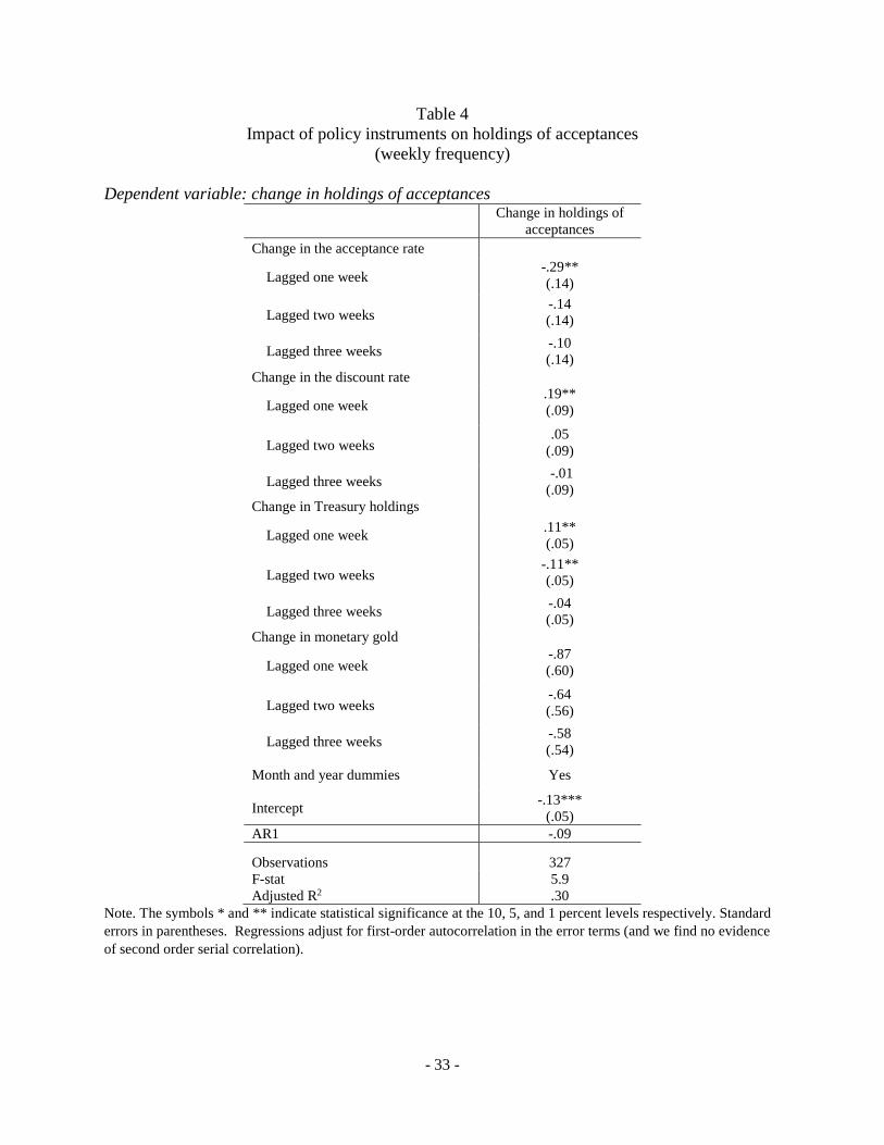
We show the results of estimating equation (1) in Table 3. Table 4 shows the results of

estimating equation (2) and Table 5 shows the results of estimating equation (3). From Table 3,

we find that the impact of a 25 basis point increase in the acceptance rate would be expected to

raise the commercial paper rate by 10.4 basis points. Based on Table 4, we estimate that a 25

basis point increase in the acceptance rate would have reduced the amount of acceptances on the

Fed’s balance sheet by about $13,200. That reduction in holdings would, based on the estimates

in Table 5, have reduced the commercial paper rate by 0.8 basis points. Thus, we find much

stronger effects from the reduction in the acceptance rate than can be accounted for by the

changes in reserves.

To test our additional hypothesis, we calculate the impact of a reduction in $13,200 of

Treasury securities and of gold. Based on the estimates in Table 3, we find that amount of

Treasury sales would have increased the commercial paper by 0.8 basis points. Similarly, that

dollar amount reduction to monetary gold would have raised the commercial paper rate by 0.8

basis points. Thus, we find evidence consistent with the idea that the same dollar amount change

in all three balance sheet items that would have impacted reserves, had the same effect on the

22 In fact, the effect of this two-step procedure should be slightly larger as banks would presumably offset some of the change in reserves due to changes in sales of acceptances to the Fed with changes in the discount window borrowing so that the overall changes in reserves is less than the change in acceptances. That offsetting effect is captured in (1) but not in (2) + (3).

- 21 -

commercial paper rate, consistent with this specification capturing the impact of the reserves

channel.

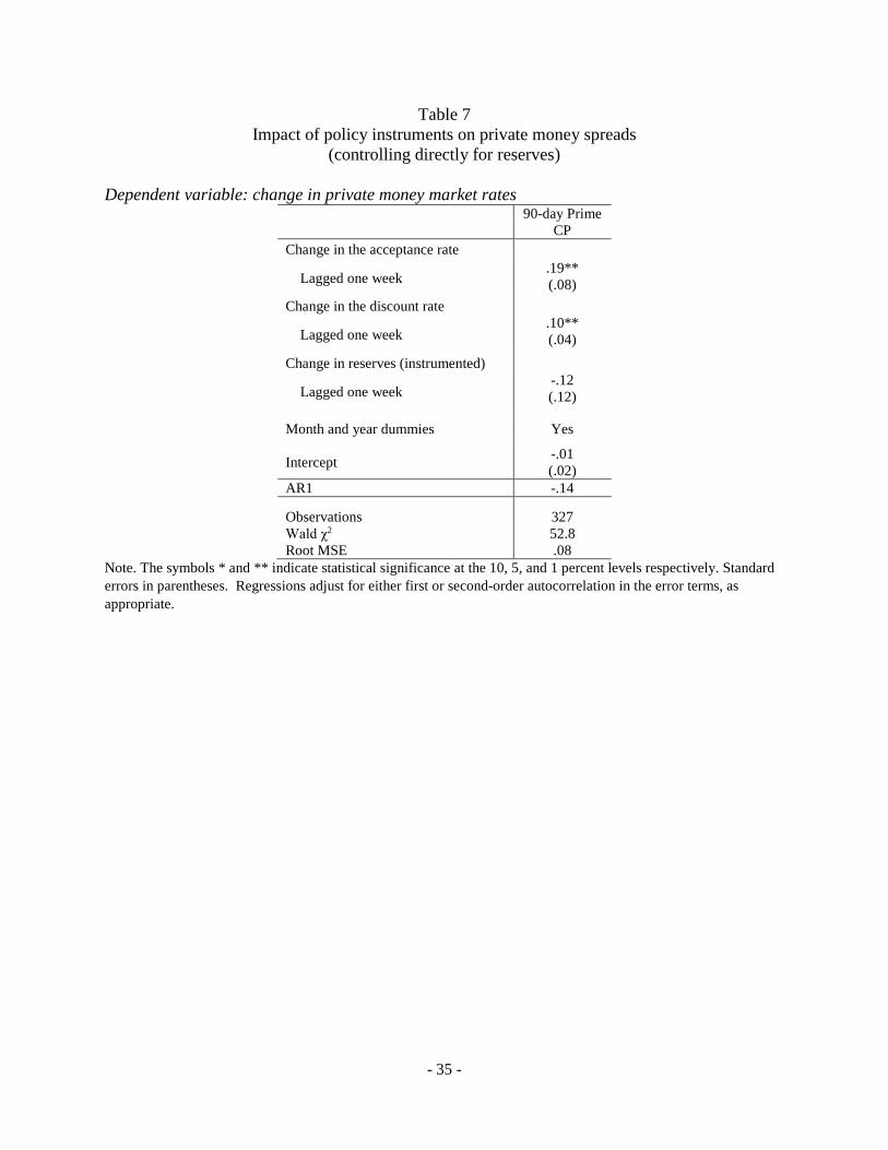
4.2 Robustness check

We confirm that the acceptance rate has effects beyond the reserves channel by

estimating the effect changes in the acceptance rate create, even after controlling for the effect of

reserves directly. We do this by regressing changes in money rates on the changes in the

acceptance rate, the change in the discount window rate and the change in reserves. Finding that

the change in the acceptance rate still matters provides a check on our earlier results.

Banks could choose to obtain reserves from the Fed by borrowing at the discount

window. They might be more interested in doing so after there had been a change in money

rates. Thus it is not clear that the change in reserves is exogenous. For this reason, we

instrument the changes in reserves using the change in monetary gold (which, on a week-to-week

basis, seem unlikely to be driven by changes in interest rates) and changes in Fed holdings of

Treasury securities (which was related to policy choices of the Open Market Investment

Committee).

The results, shown in Table 6, continue to indicate that the changes in the bankers’

acceptance rate had larger effects, even after controlling for the change in reserves directly. In

addition, the estimate on the impact of reserves suggests that a reduction of $13,200 in reserves

would have lifted the commercial paper rate by 0.6 basis points, fairly similar to the results

reported in the previous section.

4.2 Impact of growth in acceptances on commercial paper rates

If the role played by the portfolios and repricing of those portfolios in response to a shock

is correct, then we would also expect that changes in private market issuance of acceptances

should also affect commercial paper rates. This is because increased issuance of acceptances

creates additional supply of high quality liquid assets. Since the Fed pinned down the price of

these securities, we should not expect that the price of these securities would change. However,

we ought to see a change in the price of close substitutes, particularly commercial paper.

- 22 -

We test this by regressing the change in the commercial paper rate on changes in

holdings of changes in the amount of acceptances outstanding and the monetary policy variables.

We expect that increases in acceptances should push up the commercial paper rate. We estimate

this regression using monthly data owing to the frequency with which information is available

regarding acceptances outstanding. We also control for changes in economic activity using

changes in industrial production. We continue to control for month and year effects. The

results, in Table 7, suggest that increases in acceptances outstanding did impact money rates.

These results however, should be treated as tentative given the modest number of observations.

Section 5. Conclusion

In this paper, we provide an overview of the three primary tools used by the Fed to

implement monetary policy in the 1920s—the discount window, purchases of bankers’

acceptances, and purchases of government securities in the open market. These tools are fairly

similar to the more “novel” or “unconventional” tools that were introduced by the Fed. The

large scale asset purchases of Treasuries used by the Fed in the 1920s are were of a smaller scale

than the recent ones, although operations during two easing cycles in the earlier period did more

than triple the Fed’s Treasury portfolio. There are also parallels with respect to the administered

rates and their relation to the balance sheets of commercial banks. Both periods have an

administered rate that affects the rate of return to holding a highly liquid asset: the return on

holding acceptances in the 1920s was set largely by the rate at the Fed would purchase these

instruments while banks’ return to holding excess reserves in the modern period now depends on

the rate paid by the Fed. Similarly, in both periods the Fed has an administered rate that affects

banks’ cost of short-term funding: the discount window rate in the 1920s affected the costs of

short-term borrowing from the Fed while the rate on the modern overnight reverse repurchase

facility rate influences the cost to banks of borrowing in money markets by providing an

alternative instrument to institutions, such as money market funds, that also lend to the banks.23

We then show that the Fed was able to influence the private money market rates

effectively with each of these tools from an era when they were considered fairly conventional

23 Interestingly, the interest rate tools are related to quite different parts of the Fed’s balance sheet. The administered rates in the 1920s affect assets held by the Fed while the modern tools affect the cost of liabilities issued by the Fed.

- 23 -

and during ordinary times. Indeed, the impact of changes in holdings of Treasury securities were

larger in the 1920s than today. In addition, we provide evidence that the rate at which the Fed

purchased bankers’ acceptances had quite substantial effects on other interest rates, suggesting

that channels other than just the reserves channel of monetary policy were important for the

transmission of monetary policy.

- 24 -

References

Altavilla, Carlo, Giacomo Carboni, and Roberto Motto (2015). “Asset Purchase Programmes and Financial Markets: Lessons from the Euro Area,” European Central Bank Working Paper No. 1864.

American Acceptance Council (1924). “The Money Market,” Acceptance Bulletin, May. Beckhart, Benjamin (1932). The New York Money Market, Volume III: Uses of Funds, New

York: Columbia University Press Bordo, Michael and Arunima Sinha (2016). “A Lesson from the Great Depression that the Fed

Might Have Learned: A Comparison of the 1932 Open Market Purchases with Quantitative Easing.” NBER Working Paper No. 22581.

Bordo, Michael and David Wheelock (2013). “The Promise and Performance of the Federal

Reserve as Lender of Last Resort 1914-1933,” in Michael D. Bordo and William Roberds, eds., The Origins, History, and Future of the Federal Reserve: A Return to Jekyll Island, Cambridge University Press, pp. 59-98.

Burgess, W. Randolph (1936). The Reserve Banks and the Money Market, New York: Harper

and Brothers Publishers. Carlson, Mark and David Wheelock (2016). “"Did the Founding of the Federal Reserve Affect

the Vulnerability of the Interbank System to Systemic Risk?" Finance and Economics Discussion Series 2016-059. Washington: Board of Governors of the Federal Reserve System.

Carpenter, Seth and Selva Demiralp, and Zeynep Senyuz (2016). “Volatility in the Federal Funds

Market and Money Market Spreads during the Financial Crisis.” Journal of Financial Stability, August 2016, v. 25, pp. 225-33

Clarida, Richard, 2014, “Navigating the New Neutral”, Economic Outlook, PIMCO, November. D’Amico, Stefania, William English, David López-Salido, and Edward Nelson (2012). “The

Federal Reserve’s Large-Scale Asset Purchase Programmes: Rationale and Effects,” Economic Journal, vol. 122 (November), pp. 415-446.

Demiralp, Selva, Brian Preslopsky, and William Whitesell (2006). “Overnight Interbank Loan

Markets,” Journal of Economics and Business, January-February, vol. 58(1), pp. 67-83 Duffie, Darrell and Arvid Krishnamurthy (2016). “Passthrough Efficiency in the Fed’s New

Monetary Policy Setting.” Presentation at the Federal Reserve Bank of Kansas City Conference on “Designing Resilient Monetary Policy Frameworks,” Jackson Hole, Wyoming, August 26.

- 25 -

Eichengreen, Barry and Marc Flandreau (2012). “The Federal Reserve, the Bank of England, and the Rise of the Dollar as an International Currency, 1914-1939.” Open Econ Review 23: 57, doi: 10.1007/s11079-011-9217-1.

Federal Reserve (1923). Annual Report of the Federal Reserve Board, Washington DC: Federal

Reserve Board. Ferderer, J. Peter (2003). “Institutional Innovation and the Creation of Liquidity Financial

Markets: The Case of Bankers’ Acceptances, 1914-1934” The Journal of Economic History, vol. 63(3), pp. 666-694.

Friedman, Milton and Anna Schwarz (1963). A Monetary History of the United States, 1867-

1960. Princeton: Princeton University Press. Garbade, Kenneth (2014). “Direct Purchases of U.S. Treasury Securities by Federal Reserve

Banks,” Federal Reserve Bank of New York Staff Report No. 684. Gertler, Mark and Peter Karadi (2013). “QE 1 vs.2 vs. 3…: A Framework for Analyzing Large-

Scale Asset Purchases as a Monetary Policy Tool.” International Journal of Central Banking, vol. 9(1), pp. 5-53.

Goodfriend, Marvin (2014). “The Case for a Treasury-Federal Reserve Accord for Credit

Policy,” Testimony before the Subcommittee on Monetary Policy and Trade of the Committee on Financial Services, U.S. House of Representatives, Washington, D.C, March 12.

Hackley, Howard (1961). A History of the Lending Function of the Federal Reserve Banks,

Washington DC: Board of Governors of the Federal Reserve System. Hamilton, James (1997). “Measuring the Liquidity Effect,” American Economic Review, vol.

7(1), pp. 80-97. Hanes, Christopher (2006). “The Liquidity Trap and U.S. Interest Rates in the 1930s,” Journal of

Money, Credit, and Banking, vol. 38(1), pp. 163-194. Holston, Kathryn, Thomas Laubach, and John C. Williams (2016). “Measuring the Natural Rate

of Interest: International Trends and Determinants,” Federal Reserve Bank of San Francisco Working Paper, No. 2016-11.

Krishnamurthy, Arvid, Annette Vissing-Jorgensen, Simon Gilchrist, and Thomas Philippon

(2011). “The Effects of Quantitative Easing on Interest Rates: Channels and Implications for Policy,” Brookings Papers on Economic Activity, Fall, pp. 217-287.

Kroeger, Alexander, John McGowan, and Asani Sarkar (2017). “The Pre-Crisis Monetary Policy

Implementation Framework,” Federal Reserve Bank of New York Staff Reports, No. 809.

- 26 -

Meltzer, Allan (2003). A History of the Federal Reserve, Volume 1, 1913-1951. Chicago: University of Chicago Press.

New York Clearing House Association (1920). Constitution of the New York Clearing House

Association. Also Clearinghouse Rules, Scale of Fines, Collection Charges, and Holiday Laws of New York State. New York: New York Clearing House Association.

Reis, Ricardo (2016). “Funding Quantitative Easing to Target Inflation,” Presentation at the

Federal Reserve Bank of Kansas City Conference on “Designing Resilient Monetary Policy Frameworks,” Jackson Hole, Wyoming, August 26.

Reifler, Winfield (1930). Money Rates and Money Markets in the United States, New York:

Harper & Brothers Publishers. Small, David H. and James Clouse (2005). “The Scope of Monetary Policy Actions Authorized

under the Federal Reserve Act,” Topics in Macroeconomics 5: 1. Stein, Jeremy (2012). “Monetary Policy as Financial Stability Regulation,” Quarterly Journal of

Economics, vol. 127, pp. 57-95. Toma, Mark. (1989). “The Policy Effectiveness of Open Market Operations in the 1920s,”

Explorations in Economic History, 26: 99-116. Turner, Bernice (1931). The Federal Funds Market, New York: Prentice-Hall, Inc. Wheelock, David (1991). The Strategy and Consistency of Federal Reserve Monetary Policy,

1924-1933, Cambridge: Cambridge University Press. Wicker, Elmus (1966) Federal Reserve Monetary Policy 1917-1933, New York: Random House. Yellen, Janet (2016). “The Federal Reserve’s Monetary Policy Toolkit: Past Present, and

Future,” Remarks at the Federal Reserve Bank of Kansas City Conference on “Designing Resilient Monetary Policy Frameworks,” Jackson Hole, Wyoming, August 26.

- 27 -

Data Appendix The weekly Fed balance sheet is from the H.4.1 statistical release available from the Federal Reserve Bank of St. Louis FRASER website. The year-end 1926 balance sheet is from the Federal Reserve Board Annual Report for 1926. Interest rates for commercial paper, new call loans, renewed call loans, and time call loans are from the Federal Reserve’s Banking and Monetary Statistics 1914-1941. The interest rates on bankers’ acceptances which are from the Acceptance Bulletin of the American Acceptance Council. Interest rates on the Fed’s repo facility for acceptances are from Beckhart (1932). Interest rates on prime commercial loans and on loans secured by warehouse receipts are from the Federal Reserve Bulletins from the years 1923-1930. Outstanding amounts of commercial paper, broker loans, and acceptances are from the Federal Reserve’s Banking and Monetary Statistics 1914-1941. The index of industrial production is from the Board of Governors of the Federal Reserve.

- 28 -

Figure 1 Market rate of interest and FRBNY buying rate on bankers’ acceptances

Source: Federal Reserve, Banking and Monetary Statistics, 1943.

Figure 2

Holdings of Treasury Securities and the Discount Rate


0.00

1.00

2.00

3.00

4.00

5.00

6.00

12/3/1921 12/3/1922 12/3/1923 12/3/1924 12/3/1925 12/3/1926 12/3/1927 12/3/1928

Prime Bankers Acceptances (90 days) market rate FRBNY acceptance rate 61-90 days

0

100

200

300

400

500

600

700

800

2

2.5

3

3.5

4

4.5

5

5.5

6

6.5

Trea

sury

hol

dins

($ m

illio

ns)

Inte

rest

rate

s (pe

rcen

t)

Discount Rate Treasuries (right)

- 29 -

Figure 3 Federal Reserve Policy Rates and Private Money Market Rates


0.0

1.0

2.0

3.0

4.0

5.0

6.0

7.0

8.0

9.0

10.0

Inte

rest

rate

s (pe

rcen

t)

Prime CP (4-6 months) Stock time loans - 90 days

New York Fed discount rate FRBNY acceptance rate 45-60 days

- 30 -

Table 1 Balance sheet of the Federal Reserve

December 31, 1926

Assets Equity and Liabilities Gold held against Federal

Reserve notes 1,448.6 Federal Reserve Notes 1850.8

Other gold 1,369.9 Bills rediscounted Deposits

Commercial and industrial paper 170.6 Member bank reserves 2194.1

U.S. Government 1.1 Other deposits 81.9 Other bills 3.1

Advances Other liabilities 669.7 Secured by U.S.

Government 364.2

Otherwise secured 97.6 Bills bought in open market

Acceptances for imports & exports 252.2

Acceptances for domestic trade 77.7

Other bills 51.0 US Gov. securities bought in open market

Certificates of indebtedness 179.5 Notes 87.4 Bonds 48.0

Uncollected items 730.5 Capital 124.8 Surplus 228.8 Other assets 268.7 Total 5150.1 Total 5150.1

Note. All values in millions of dollars.

- 31 -

Table 2 Summary statistics

Weekly variables

Variable Obs. Mean Standard Deviation Min Max

Change in the commercial paper rate (basis pts) 314 .31 6.9 -37 25

Change in the call loan time rate (basis pts) 314 1.2 15.2 -63 100

Change in the call loan renewal rate (basis pts) 314 .68 74 -390 435

Change in the discount window rate (basis pts) 314 .47 10.9 -50 100

Change in the rate on acceptances with 30-45 days to maturity (basis pts) 314 .36 737 -50 38

Change in holdings of Treasury securities ($100,000) 314 -.005 .25 -1.76 1.07

Change in holdings of acceptances ($100,000) 314 -.004 .20 -.65 .74

Change in holdings of gold ($1,000,000) 314 -.0002 .02 -.07 .07

Monthly variables Variable Obs. Mean Standard

Deviation Min Max

Change in the commercial paper rate (basis pts) 83 .49 19.9 -74.7 44.4

Change in the discount window rate (basis pts) 83 .60 23.6 -130 80

Change in the rate on acceptances with 30-45 days to maturity (basis pts) 83 .14 19.7 -76.5 58.8

Change in holdings of Treasury securities ($100,000) 83 .0001 .05 -.12 .17

Change in holdings of gold ($1,000,000) 83 -.002 .04 -.12 .08

Change in bankers acceptances outstanding ($100,000,000) 83 .11 .63 -1.3 2.7

Change in IP 81 1.1 .11 .90 1.42

- 32 -

Table 3 Impact of policy instruments on changes in private money rates

(weekly frequency)

Dependent variable: change in the private money market rates 90-day Prime

CP

Call loans on time

(90-day)

Call loans renewal

Change in the acceptance rate

Lagged one week .21*** (.05)

.23** (.12)

.01 (.38)

Lagged two weeks .09* (.05)

.08 (.12)

.21 (.41)

Lagged three weeks .12** (.05)

.07 (.12)

.61* (.37)

Change in the discount rate


.10 (.08)

.03 (.34)

Lagged two weeks -.02 (.03)

-.02 (.08)

-.14 (.30)

Lagged three weeks .02 (.03)

-.11 (.08)

-.31 (.30)

Change in Treasury holdings

Lagged one week -.01 (.02)

-.001 (.04)

.20 (.12)

Lagged two weeks -.03* (.02)

-.12*** (.04)

-.37*** (.13)

Lagged three weeks -.02 (.02)

-.02 (.04)

-.14 (.13)

Change in monetary gold


-.15 (.50)

-5.7*** (1.6)

Lagged two weeks -.52***

(.20) -1.04**

(.47) -3.4** (1.6)


-.59 (.45)

4.9*** (1.4)

Month and year dummies Yes Yes Yes

Intercept -.03* (.02)

-.02 (.03)

-.28*** (.10)

AR1 -.14 .12 -.40

Observations 327 327 304 F-stat 4.8 1.7 5.2 Adjusted R2 .25 .06 .28

Note. The symbols * and ** indicate statistical significance at the 10, 5, and 1 percent levels respectively. Standard errors in parentheses. Regressions adjust for first-order autocorrelation in the error terms (and we find no evidence of second order serial correlation).

- 33 -

Table 4 Impact of policy instruments on holdings of acceptances

(weekly frequency)

Dependent variable: change in holdings of acceptances Change in holdings of

acceptances Change in the acceptance rate

Lagged one week -.29** (.14)




Lagged one week .19** (.09)

Lagged two weeks .05

(.09)




Lagged two weeks -.11** (.05)






Month and year dummies Yes

Intercept -.13*** (.05)

AR1 -.09

Observations 327 F-stat 5.9 Adjusted R2 .30


- 34 -

Table 5 Impact of policy instruments on changes in private money rates

(weekly frequency)

Dependent variable: change in the private money market rates 90-day Prime

CP

Call loans on time

(90-day)

Call loans renewal

Change in acceptance holdings

Lagged one week -.04** (.02)

.03 (.05)

.63*** (.14)


.02 (.05)

-.24* (.15)


-.11** (.05)

-.52*** (.37)



.13* (.08)

.04 (.26)

Lagged two weeks .03

(.03) .04

(.08) .09

(.26)

Lagged three weeks .06* (.03)

-.06 (.08)

.06 (.26)



-.02 (.04)

.05 (.12)


(.02) -.14***

(.04) -.34***

(.12)

Lagged three weeks -.03* (.02)

-.001 (.04)

-.11 (.13)



-.05 (.50)

-5.3*** (1.5)


(.21) -.99** (.48)

-2.6** (1.5)


-.78* (.46)

2.9** (1.4)

Month and year dummies Yes Yes Yes

Intercept -.03* (.02)

-.04 (.05)

-.27*** (.10)

AR1 -.07 .13 -.36

Observations 327 327 304 F-stat 3.2 1.8 6.7 Adjusted R2 .16 .07 .35


- 35 -

Table 7 Impact of policy instruments on private money spreads

(controlling directly for reserves)

Dependent variable: change in private money market rates 90-day Prime

CP Change in the acceptance rate




Change in reserves (instrumented)


Month and year dummies Yes

Intercept -.01 (.02)

AR1 -.14

Observations 327 Wald χ2 52.8 Root MSE .08

Note. The symbols * and ** indicate statistical significance at the 10, 5, and 1 percent levels respectively. Standard errors in parentheses. Regressions adjust for either first or second-order autocorrelation in the error terms, as appropriate.

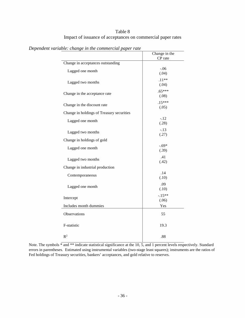
- 36 -

Table 8 Impact of issuance of acceptances on commercial paper rates

Dependent variable: change in the commercial paper rate

Change in the CP rate

Change in acceptances outstanding

Lagged one month -.06 (.04)

Lagged two months .11** (.04)

Change in the acceptance rate .65*** (.08)

Change in the discount rate .15*** (.05)

Change in holdings of Treasury securities

Lagged one month -.12 (.28)

Lagged two months -.13 (.27)

Change in holdings of gold

Lagged one month -.69* (.39)

Lagged two months .41 (.42)

Change in industrial production

Contemporaneous .14 (.10)

Lagged one month .09 (.10)

Intercept -.15** (.06)

Includes month dummies Yes

Observations 55

F-statistic 19.3

R2 .88

Note. The symbols * and ** indicate statistical significance at the 10, 5, and 1 percent levels respectively. Standard errors in parentheses. Estimated using instrumental variables (two-stage least squares); instruments are the ratios of Fed holdings of Treasury securities, bankers’ acceptances, and gold relative to reserves.

“unconventional” monetary policy as conventional...

Documents