undergraduate research thesis
TRANSCRIPT

School of Chemical Engineering
CHEMENG 4054 Research Project
A New Risk Assessment for Microbiologically Influenced Corrosion of
Metals
Connor Skoss
Principal supervisor: Kenneth Davey
Co-supervisor: Samuel D. Collins
School of Chemical Engineering, University of Adelaide, Adelaide, SA 5005
Abstract
Microbiologically Influenced corrosion (MIC) is an electrochemically driven form of
corrosion that is initiated by the presence of microbial activity, which can lead to failure of
metals in chemical engineering processes. Existing risk assessment methods have several
disadvantages in being highly dependent on specific microorganism-metal systems, and do
not account for fluctuations in bacterial behaviour. A simplified MIC model was developed,
and is used for a new risk assessment of MIC using a probabilistic based risk framework that
can quantify random fluctuations as a distribution. This assessment was conducted for a
carbon-steel pipeline at standard operating conditions. The findings of this new risk
assessment framework were compared with traditional methods and found to offer significant
improvements by determining the frequency that MIC would occur over a particular operating
period. These findings have application to a wide range of industries involved in metal
selection and fluid flow through process equipment.
Keywords: carbon-steel pipe corrosion; Single Value Assessment (SVA); Fr13 risk
modelling; Microbiologically Influenced Corrosion (MIC)

Page 2 of 39
1.0 Introduction
This project uses a new risk assessment method for the microbiologically influenced
corrosion (MIC) of metals. Microbiological influenced corrosion (MIC) is an
electrochemically driven form of corrosion, which is influenced by the presence of
microorganisms. These microorganisms induce extensive pitting corrosion on the surface of
metals that significantly reduces equipment lifespan, and causes premature failures,
collectively costing the oil and gas industry $100 million globally (Javaherdashti et al., 2011).
The motivation of this project is to examine if the new risk methodology, the Friday 13th (Fr
13) framework, improving upon the practical limitations of existing mechanistic corrosion
risk models that do not adequately quantify the occurrence of natural fluctuations in steady-
state processes. This work is significant in being the first to attempt to develop a
comprehensive MIC risk assessment methodology that quantifies potential risk as a
distribution related to steady-state process parameters.
This project aims replicate the work undertaken by Collins et al. (2016), and extends upon the
limitations of this work. These include using an abiotic corrosion model to model biotic
bacterial corrosion behavior, and developing a more justified method of calculating Ecorr as a
multi-variable function of temperature and pH. These aims will be achieved using Fr 13, a
probabilistic risk assessment framework developed by Davey and others that quantifies
random fluctuations within a process, along with probability of a particular value physically
occurring. Using refined Monte Carlo (r- MC) sampling of the distributions ensures sampling
covers the entire range of the distribution and accounts for all possible scenarios. Analysis of
these distributions will allow the identification, of which process variables are the driving
parameters of MIC, and through second tier studies, how process changes can be implemented
to reduce the occurrence of MIC inducing an equipment failure.
2.0 Literature review
Studies on the effects of MIC were first motivated by the extensive corrosion in Holland’s
steel pipe waterways during the 1930s. Von Wolzogen Kuhr and Van der Flught (1934)
conducted an experiment to determine the origin of the corrosion. Having identified the
presence of sulphate reducing bacteria (SRB) within the river water samples, the authors
postulated the cathodic depolarisation theory (CDT) as the mechanism for how bacteria
groups such as SRB influence the corrosion of metals.

Page 3 of 39
In following studies several authors challenged CDT as an appropriate mechanistic model for
MIC. Wanklyn and Spruit (1951) examined SRB’s consumption of H2 in cathodic
depolarization leading to iron corrosion, and determined CDT did not adequately explain the
cathode charge measurements. In contrast, Iverson (1966) used the basis of Wanklyn and
Spruit’s study to further assess the validity of CDT by using cultured SRB in agar gel in a
nitrogen atmosphere, investigated several different types of metals. Iverson found the rate of
corrosion was smaller than anticipated, and unable to be fully attributed to CDT, but surmised
the broad theory was valid. The study was significant as being the first to develop a simple
corrosion model based on the experimental results.
De Waard et al. (1991) developed the deWaard-Milliams carbon dioxide corrosion model for
use in natural gas pipelines. Although not focused on MIC, the methodology for corrosion
modelling used by De Waard et al. (1991) provided a basis for further MIC studies that
shifted focus from assessing microorganism’s corrosion mechanisms, to creating a corrosion
model for MIC risk assessment. Pots et al. (2002) expanded upon the de Waard-Milliams
model to create a specific MIC corrosion that was incorporated into the HYDROCOR risk
assessment software. A key limitation of the Pots et al. (2002) model was the lack of
incorporation of appropriate biochemical parameters into the mechanistic model, which
affected the model accuracy. Studies by Maxwell and Campbell (2006) attempted to address
the limitation of the Pots et al. (2002) model by expanding the biochemical parameters used in
the model along with first-order bacterial kinetics to describe the sulfur-based biofilm growth
during the initial stages of MIC. The resultant modified model produced comparative results
to that of the original Pots et al. (2002) model, whilst the inclusion of bacterial kinetics
reduced the number of corrosion parameters from 11 to 4. Additionally, integration of the
bacterial kinetics helped address the initial problems by allowing the bacteria life cycle and
relative biocide effectiveness to be quantified. Smith et al. (2011) recognised the extensive
biochemical parameters associated with MIC was a large limitation in previous studies, and
investigated improving model accuracy through using a more appropriate model. This model
was fundamentally based around the Butler-Volmer kinetics to describe ion charge transfer.
Additionally, the Nernst diffusion model was incorporated to account for the mass transfer
process occurring during the corrosion. The resultant model produced reasonable qualitative
likeness with experimental data near the corrosion potential. However it was observed that a
larger overpotential in the system created more deviations between the model and
experimental values.

Page 4 of 39
Common issues with many of the models and generalised results, highlighted by the work of
Pots et al. (2002) and Maxwell and Campbell (2006), is that the mechanistic corrosion models
constructed were not sophisticated enough to take into account all the biological parameters.
These were compensated by making simplistic assumptions for biological variables that
cannot be accounted for in the models. This substantially reduces the accuracy and usefulness
of these models as a risk assessment tool. Both are unable to incorporate key variables as well
as not being able to quantify the natural fluctuations these variables undergo within the
system. Another issue noted is that in studies such as Smith et al. (2011), little analysis was
undertaken on how well the simulated MIC environment mimics MIC in real life, and how the
general findings can be applied. Lastly, the majority of studies almost exclusively focused on
the effects of SRB, where increasing evidence has shown APB to present equal, if not more
risk than SRB. This limits the effectiveness of the development of a corrosion risk model that
can accurately account for the effects from all the main corrosion inducing bacteria groups.
The traditional method used to create an MIC risk model is to use a deterministic approach to
solve a certain outcome, in this case occurrence of corrosion. The approach of linking the
operation parameters together in a mathematical expression and solving to find a particular
output is also known as Single Value Assessment (SVA) (Davey and Cerf, 2003). The use of
the deterministic SVA method has been the primary method employed by all previous work
used in developing an MIC risk model, including De Waard et al. (1991), Pots et al. (2002),
and Maxwell and Campbell (2006). The fundamental flaw with the use of SVA in chemical
engineering processes is that naturally occurring random fluctuations in inputs and their
potential impact on plant outcome behaviour cannot be implicitly accounted for, or quantified
using SVA (Davey and Zou, 2015). Although a new risk modelling methodology, several
studies have successfully used the Fr 13-risk assessment framework for steady state, single-
step unit-operations processes. These studies have not examined MIC specifically, however
lessons can be observed from the study’s findings and application of Fr 13 in terms of how is
could best be applied to further research on MIC.
The Fr 13 framework was used in the work undertaken by Davey (2015) to assess the fuel-to-
steam thermal efficiency of a coal-fired boiler (CFB), used to examine the potential risk of
reduced CFB efficiency from naturally occurring fluctuations. The unit-operations model was
used to simulate 20 key efficiency related parameters. The findings of the Fr 13 simulations
determined that 73 failures in CFB efficiency occurred per 10,000 operations. Further
sensitivity analysis determined that the undesirable impact on efficiency from fluctuations

Page 5 of 39
could be reduced by ensuring the consistency of the size and mixture of the coal be improved
across several feed batches.
Through its use in several different fields of chemical processing, the Fr 13-risk framework
has been able to significantly improve upon the use of the traditional SVA to conduct risk
analysis. Furthermore, the quantitative results produced using the MC method have a number
of advantages over other probabilistic risk analysis methods (Milazzo and Aven, 2012),
principally due to the ability to pinpoint individual parameters that are influencing the
processes failure rate, and then conduct second-tier simulations to target these parameters by
implementing design changes. A current limitation of Fr 13 is that the methodology is
generally limited to single step unit operations and hence may not be suitable for multi-step
unit operation processes (Davey and Zou, 2015). Based on various studies undertaken using
Fr13, there is no evidence that suggests the Fr 13 framework is unsuitable to be applied in
conducting a risk assessment for MIC using a single unit operation model.
3.0 Method
A summary of the primary project tasks is described below:
1. Synthesise an abiotic MIC model based upon a simplified version of the Smith et al. (2011)
model and address the key limitation of the work of Collins et al. (2016) by creating a solver
loop to develop a more justified method of calculating Ecorr (free corrosion potential)
2. Solve the abiotic unit-operation model using the deterministic method of single value
assessment (SVA) using fixed values for temperature and pH. Then solve using the
probabilistic Fr 13 framework of Davey and co-workers
3. Compare and validate results against of other established corrosion models
4. Use the Fr 13 methodology to gain new insights into how random fluctuations affect MIC
through manipulating the input variables of temperature and pH
5. Determine the requirements to allow the abiotic corrosion model to be modified such that it
can become a biotic corrosion model, which will enhance the applicability of the risk model.

Page 6 of 39
3.1 Synthesis of Unit Operation Model
The generalised unit operation model will be heavily based upon the model constructed by
Smith et al. (2011) and the further modifications made by Collins (2016). The three-electrode
corrosion cell and potentiostat model of Smith et al. (2011) provides a realistic basis for
synthesis of a simplified unit-operations model of MIC corrosion, Fig. 1. The model is a
simplified version of steel corrosion subjected to synthetic water as MIC presented by Smith
et al. (2011).
Fig. 1 – Schematic of the three-electrode cell with synthetic water reproduced from Smith et
al. 2011)
The unit-operation model was derived using a system of linear equations based around the
Butler-Volmer kinetics, which described the charge transfer of the oxidation of iron along
with the Nernst diffusion model for the mass transfer process occurring during the corrosion
process. Complete breakdown of the unit-operation model is demonstrated in Appendix A.
It is assumed that the electrons formed by the oxidation of iron in the steel (Eq. [1]) are
consumed by the reduction of protons (Eq. [2]):
𝐹𝑒 → 𝐹𝑒!! + 2𝑒! [1]
𝐻! + 𝑒! → !!𝐻! [2]

Page 7 of 39
The transfer of charge (electrons) occurs only at the steel surface between the steel and the
water (electrolyte) because of the nature of electron transport. The overall corrosion reaction
is:
𝐹𝑒 + 2𝐻! → 𝐹𝑒!! + 𝐻! [3]
The charge transfer at the steel surface can be described by the Butler-Volmer equation (Gu,
2009) for current density due to the oxidation of iron (anodic process)
𝑗!",!! = 𝑗!,!! 𝑒𝑥𝑝!!,!! ∙!!! ∙!
!∙!∙ 𝜂!! − 𝑒𝑥𝑝
!!!,!! ∙!!! ∙!
!∙!∙ 𝜂!! [4]
From the expanded unit operation model in Appendix A, a simplified expression for MIC of a
carbon steel pipe can be described through Eq. [13], where 𝑗!" is equivalent to the number of
electrons produced in the oxidation of iron:
𝐶𝑅 = 1.155𝑗!" [13]
3.2 Single Value Assessment The unit-operation model-describing MIC for iron was solved using the deterministic and
single value assessment (SVA) (Sinnott, 2005; Davey, 2015). This is based on the use of
synthetic water using the two experimental input conditions detailed in Smith et al. (2011) of
T = 293.15 K and pH = 5.15. The output of this SVA is the corrosion rate of the carbon steel
pipe in mm yr-1.
Ones of the aims of this project is to address a limitation of the original work of Collins et al.
(2016), where Ecorr (free corrosion potential) was an assumed constant of -0.616 V vs SCE.
Ecorr is a multivariable function of temperature and pH, therefore this work attempted to
improve the accuracy of the findings by developing a more justifiable, calculated value of
Ecorr that will change if the input values of temperature and pH are varied. This was achieved
by creating a solver loop based around using the following Eq. [10] for overall charge
transfer, where the solver will converge on a value as close as possible to zero.
𝑗! = 𝑗!" + 𝑗!! = 0 [10]

Page 8 of 39
A domain was set such that Ecorr will only take values between - 0.4 and -1, the maximum
theoretical range Ecorr will take. Additionally, a parameter was set such that the Cs,Fe, surface
concentration of iron is always greater then Cb,,Fe, the concentration of iron in bulk solutions.
Any values that do not meet this constraint signify corrosion is no longer occurring. The
solver function is embedded within the Excel spreadsheet of the SVA. Each time an input
variable of temperature or pH is altered, the solver must be run to recalculate Ecorr. A
complete breakdown of the solver function, including instructions for use can be found in
Appendix B.
3.3 Friday 13th Framework
After the unit-operation model had been solved using the deterministic SVA method, it was
then solved using the probabilistic Fr 13 framework, and the two methods were compared.
The Fr 13 simulation (Davey et al. 2015) differs from the SVA method by considering input
parameters as distributions of values to mimic naturally occurring fluctuations within the
process, along with the probability of a particular value actually occurring. As with the SVA,
an output of the corrosion rate of the carbon steel pipe will be produced. However this output
will also be a distribution of particular outcomes that will include both desirable and
undesirable outcomes, i.e. intolerable levels of MIC.
A modified Monte Carlo (r-MC) (with Latin Hypercube) sampling of the distributions is used
to ensure sampling covers the entire range of the distribution. Vose (2008) determined the
standard MC sampling is unreliable due to its tendency to over-and under-estimate portions of
the distribution. When the sample size is large enough, the output distribution will be
approximately normal (Davey, 2015; Vose, 2008). For the simulations conducted in this
project 10 000 samples are considered sufficient (Collins et al., 2015).
As part of the Fr 13 framework a risk factor term, p, must be created to define which
outcomes in the distribution are desirable or not. This is called creating a failure definition.
For this work, a failure will be defined as any magnitude of MIC occurring, for all values p >
0 in the output distribution. This definition for a failure through the risk factor, p, can be
expressed in Eq. [14] below, where C𝑅′ is the corrosion obtained from the probabilistic Fr 13
simulation, and CR is the corrosion found in the SVA.
𝑝 = 𝐶𝑅′− 𝐶𝑅 [14]

Page 9 of 39
Eq. [14] is convenient because for all values p > 0, the corrosion is greater than acceptable.
However the definition of p can be further refined to more precisely describe MIC.
A more suitable mathematical form of the corrosion risk factor (Abdul-Halim & Davey, 2015;
Davey et al., 2015) can be expressed by Eq. [15].
𝑝 = 100 !"!
!"− 1 [15]
Eq. [15] can be considered more useful then Eq. [14], as it is dimensionless and because
corrosion rates greater than acceptable (i.e. failures) can be readily identified for all values p >
0. However, Eq. [15] can lastly be modified by including a measure of tolerance, shown in
Eq. [16], as a factor of design safety. There is no tolerance recommendation or guidelines
within the oil and gas industry, in the absence of conditional data, a tolerance of 25 % will be
used initially for all simulations. Part of this work will include examining the impact of
different tolerance levels. Eq. [16] will be used to define risk factor of the probabilistic Fr 13
model of MIC of the steel pipeline in water.
𝑝 = 100 !"!
!"− 1 −%𝑡𝑜𝑙𝑒𝑟𝑎𝑛𝑐𝑒 [16]
Computations for the Fr 13-risk model to determine the corrosion rate are to be carried out
using Microsoft Excel™ with a commercially available add-on @Risk™ (version 7.5,
Palisade Corporation). Excel is chosen as it is widely available and is generally well
understood across both academic and industry sectors. Furthermore, the distributions defining
naturally occurring fluctuations in the parameters can be manipulated using Excel formulae
(Abdul-Halim and Davey, 2016).
3.4 Second Tier Studies
The findings from the Fr 13 simulations may permit further insight into MIC of metals
through second tier studies (Davey, 2015) that aim to change an input parameter to reduce
failure rate. Several physical and chemical methods are used to remove or inactivate corrosion
inducing bacteria; one chemical method involves adding chlorine gas to the pipeline where it

Page 10 of 39
dissolves in the water to form hypochlorous acid (HOCl) and hyperchlorite (OCl-1) at
equilibrium of pH 7.5 (Tuthill et al., 1998). The addition of chlorine gas to the pipeline will
be simulated in the model by increasing the pH to 7.5.
This second tier study will also involve assessing the abiotic models responsiveness to pH
change by running a simulation at pH 3 where corrosion inducing bacteria should
theoretically thrive. The model will be solved with both SVA and the Fr 13 framework to
allow insight into whether or not the abiotic corrosion model can adequately model bacterial
fluctuations.
4.0 Results
Simulations were run in Microsoft Excel™ using the commercial add-on @Risk™. A
simulation was conducted for mid-range operating conditions commonly found in oil and gas
pipelines. Two simulations were then undertaken as second tier studies. The first was to
assess the effects of simulating the addition of chlorine gas to a pipeline to inactivate
corrosion inducing bacteria. The second simulation aimed to replicate ideal bacterial
conditions by reducing the pH 3. Each of these three simulations were then used to analyse
the effect tolerance has on failure rate by repeating each simulation at 0 % and 50 %
tolerance. These simulations analysing tolerance can be found in Appendix C.
For each a simulation a summary table of the comparison of results produced from the
traditional SVA and the new Fr 13 simulation was generated. Rows 2 and 3-show
temperature and pH, the two model input parameters that are prone to natural fluctuations.
The physical system is fixed by constant parameters shown in rows 6 to 28. These constant
parameters, along with the input parameters were used to determine the calculated values
shown in rows 31 through to 46. The traditional SVA is read down column 2 where the
corrosion rate an annual figure of the corrosion of the carbon steel pipe (mm yr-1) is the output
in row 48. Meanwhile, the Fr 13 simulation is read down column 4 in which a normal
distribution has been used for both T and pH. These are represented by the @risk commands:
RiskNormal (mean, stdev, RiskTruncate(minimum, maximum)), these distributions model
how in operation the temperature and pH within a pipeline will vary randomly, but not outside
a certain range. Additionally, for each simulation a Risk Factor, p, distribution plot was
produced. This uses the definition that a failure, i.e. corrosion occurring, is represented by all

Page 11 of 39
values p > 0 to depict the amount of failures that would occur due to random fluctuations of
the input parameters, temperature and pH. The x-axis is the computed value of p from Eq.
[15] whilst the y-axis is the probability of p actually occurring.
Table 1 presents a summary comparison of results from the orthodox SVA and the new Fr 13
simulation of MIC of a carbon steel pipe at mid-range operating conditions of T = 293.15 K,
and pH = 5.15 for rows 2 and 3 respectively. The SVA output was 0.45 mm yr-1. The Fr 13
simulation, using a tolerance of 25 %, produced the same corrosion output as the SVA, whilst
these particular input parameter conditions produced a p value of 25. The corresponding
distribution of p values is shown in Fig. 1, which shows that from the 10 000 samples of
different temperature and pH values, 25 % or 2500 failures occurred. Shown in Appendix C
for Figs. C1 and C2, when using tolerances of 0 % and 50% for the Fr 13 simulations, failure
rate was found to be 50 % and 9 % respectively.

Page 12 of 39
Table 1 – SVA and Fr 13 Results (T = 293.15 K, pH = 5.15, Tolerance = 25 %)
Row Parameter SVA Fr 13 Simulation 1 Input 2 T (K) 293.15 293.15
RiskNormal(293.15,29.3,RiskTruncate(263.835,322.465))
3 pH 5.15 5.15 RiskNormal(5.15,0.515,RiskTruncate(4.63
5,5.665)) 4 5 Constants 6 αa,Fe (dimensionless) 0.4 0.4 Constant 7 αa,H+ (dimensionless) 0.6 0.6 Constant 8 αc,Fe (dimensionless) 0.6 0.6 Constant 9 αc,H+ (dimensionless) 0.4 0.4 Constant
10 nFe (dimensionless) 2 2 Constant 11 nH+ (dimensionless) 1 1 Constant 12 e(0,Fe) (A) 1.00E-07 1.00E-07 Constant 13 e(0,H+) (A) 1.00E-07 1.00E-07 Constant 14 A,E (m^2) 2.83E-03 2.83E-03 Constant 15 𝛾,Fe (dimensionless) 0.3 0.3 Constant 16 𝛾,H+ (dimensionless) 0.75 0.75 Constant 17 E°Fe (V vs SCE) -0.681 -0.681 Constant 18 E°H+ (V vs SCE) -0.241 -0.241 Constant 19 Cs,Fe (mol m-3) 1.00E-03 1.00E-03 Constant 20 Cs,H+ (mol m-3) 1.00E-07 1.00E-07 Constant 21 Cb,Fe (mol m-3) 1.01E-05 1.01E-05 Constant 22 DFe (m2 s-1) 7.98E-10 7.98E-10 Constant 23 DH+ (m2 s-1) 9.47E-09 9.47E-09 Constant 24 δN,Fe (m2) 7.23E-06 7.23E-06 Constant 25 δN,H+ (m2) 1.67E-05 1.67E-05 Constant 26 F (C mol-1) 96485 96485 Constant 27 R (J mol-1 K-1) 8.314 8.314 Constant 28 Tolerance (%) - 25 29 30 Calculations 31 Cb,H+ (mol m3) 7.08E-03 7.08E-03 Eq. [1] 32 j0,Fe (A m-2) 1.40E-04 1.40E-04 Eq. [5] 33 j0,H+ (A m-2) 0.00 0.00 Eq. [7] 34 Erev,Fe (V vs SCE) -7.68E-01 -7.68E-01 Eq. [6] 35 Erev,H+ (V vs SCE) -6.48E-01 -6.48E-01 Eq. [4] 36 jmt,Fe (A m2) 2.11E-02 2.11E-02 Eq. [9] 37 jmt,H+ (A m2) -3.87E-01 -0.387335386 Eq. [10] 38 jct,Fe (A m2) 3.66E-01 3.66E-01 Eq. [11] 39 jct,H+(A m2) 0.00 0.00 40 ηFe (V vs SCE) 2.48E-01 2.48E-01 41 ηH+ (V vs SCE) 0.13 0.13 Eq. [13] 42 Ecorr (V vs. SCE) -0.52 -0.52 43 jFe (A m-2) 0.39 0.39 Eq. [6] 44 jH+ (A m-2) -0.39 -0.39 Eq. [6] 45 jT (A m-2) 0.00 0.00 Eq. [6] 46 0.00 0.00 Eq. [6] 47 Output 48 CR (mm yr-1) 0.45 0.45 Eq. [13] 49 50 p - 25.00 Eq. [16]
Page 13 of 39
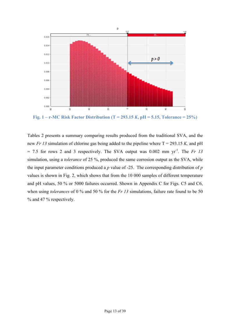
Fig. 1 – r-MC Risk Factor Distribution (T = 293.15 K, pH = 5.15, Tolerance = 25%)
Tables 2 presents a summary comparing results produced from the traditional SVA, and the
new Fr 13 simulation of chlorine gas being added to the pipeline where T = 293.15 K, and pH
= 7.5 for rows 2 and 3 respectively. The SVA output was 0.002 mm yr-1. The Fr 13
simulation, using a tolerance of 25 %, produced the same corrosion output as the SVA, while
the input parameter conditions produced a p value of -25. The corresponding distribution of p
values is shown in Fig. 2, which shows that from the 10 000 samples of different temperature
and pH values, 50 % or 5000 failures occurred. Shown in Appendix C for Figs. C5 and C6,
when using tolerances of 0 % and 50 % for the Fr 13 simulations, failure rate found to be 50
% and 47 % respectively.

Page 14 of 39
Table 2 – SVA and Fr 13 Results (T = 293.15 K, pH =7.5, Tolerance = 25 %)
Row Parameter SVA Fr 13 Simulation 1 Input 2 T (K) 293.15 293.15
RiskNormal(293.15,29.3,RiskTruncate(263.835,322.465))
3 pH 7.5 7.64 RiskNormal(7.5,0.75,RiskTruncate(6.95,8.4
5)) 4 5 Constants 6 αa,Fe (dimensionless) 0.4 0.4 Constant 7 αa,H+ (dimensionless) 0.6 0.6 Constant 8 αc,Fe (dimensionless) 0.6 0.6 Constant 9 αc,H+ (dimensionless) 0.4 0.4 Constant
10 nFe (dimensionless) 2 2 Constant 11 nH+ (dimensionless) 1 1 Constant 12 e(0,Fe) (A) 1.00E-07 1.00E-07 Constant 13 e(0,H+) (A) 1.00E-07 1.00E-07 Constant 14 A,E (m^2) 2.83E-03 2.83E-03 Constant 15 𝛾,Fe (dimensionless) 0.3 0.3 Constant 16 𝛾,H+ (dimensionless) 0.75 0.75 Constant 17 E°Fe (V vs SCE) -0.681 -0.681 Constant 18 E°H+ (V vs SCE) -0.241 -0.241 Constant 19 Cs,Fe (mol m-3) 1.00E-03 1.00E-03 Constant 20 Cs,H+ (mol m-3) 1.00E-07 1.00E-07 Constant 21 Cb,Fe (mol m-3) 1.01E-05 1.01E-05 Constant 22 DFe (m2 s-1) 7.98E-10 7.98E-10 Constant 23 DH+ (m2 s-1) 9.47E-09 9.47E-09 Constant 24 δN,Fe (m2) 7.23E-06 7.23E-06 Constant 25 δN,H+ (m2) 1.67E-05 1.67E-05 Constant 26 F (C mol-1) 96485 96485 Constant 27 R (J mol-1 K-1) 8.314 8.314 Constant 28 Tolerance (%) - 25 29 30 Calculations 31 Cb,H+ (mol m3) 3.16E-05 2.28E-05 Eq. [1] 32 j0,Fe (A m-2) 1.40E-04 1.40E-04 Eq. [5] 33 j0,H+ (A m-2) 0.00 0.00 Eq. [7]
34 Erev,Fe (V vs SCE) -7.68E-01 -7.68E-01 Eq. [6]
35 Erev,H+ (V vs SCE) -6.48E-01 -6.48E-01 Eq. [4]
36 jmt,Fe (A m2) 2.11E-02 2.11E-02 Eq. [9]
37 jmt,H+ (A m2) -1.72E-03
-0.001242217 Eq. [10]
38 jct,Fe (A m2) -1.93E-02 -1.93E-02 Eq. [11]
39 jct,H+(A m2) 0.00 0.00 40 ηFe (V vs SCE) -1.04E-
01 -1.04E-01 41 ηH+ (V vs SCE) -0.22 -0.22 Eq. [13] 42 Ecorr (V vs. SCE) -0.87 -0.87 43 jFe (A m-2) 0.00 0.00 Eq. [6] 44 jH+ (A m-2) 0.00 0.00 Eq. [6] 45 jT (A m-2) 0.00 0.00 Eq. [6] 46 0.00 0.00 Eq. [6] 47 Output 48 CR (mm yr-1) 0.0020 0.002 Eq. [13] 49 50 p - -25.00 Eq. [16]

Page 15 of 39
Fig. 2 – r-MC Risk Factor Distribution (T = 293.15 K, pH =7.5, Tolerance = 25%)
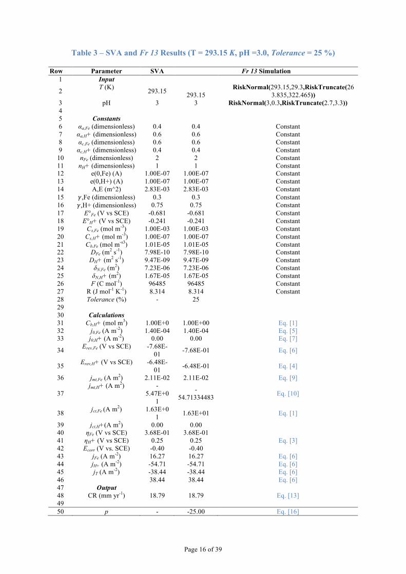
Tables 3 presents a summary comparison of results produced from the traditional SVA and
the new Fr 13 framework simulating ideal bacterial pH conditions where T = 293.15 K, and
pH = 3 for rows 2 and 3 respectively. The SVA output was 18.79 mm yr-1. The Fr 13
simulation, using a tolerance of 25 %, produced the same corrosion output as the SVA, whilst
the input parameter conditions produced a p value of -25. The corresponding distribution of p
values is shown in Figure 2, which shows that from the 10 000 samples of different
temperature and pH values, 35 % or 3500 failures occurred. Shown in Appendix C for Figs.
C3 and C4, when using tolerances of 0 % and 50 % for the Fr 13 simulations, failure rate was
found to be 50 % and 25 % respectively.
Page 16 of 39
Table 3 – SVA and Fr 13 Results (T = 293.15 K, pH =3.0, Tolerance = 25 %)
Row Parameter SVA Fr 13 Simulation 1 Input 2 T (K) 293.15 293.15
RiskNormal(293.15,29.3,RiskTruncate(263.835,322.465))
3 pH 3 3 RiskNormal(3,0.3,RiskTruncate(2.7,3.3)) 4 5 Constants 6 αa,Fe (dimensionless) 0.4 0.4 Constant 7 αa,H+ (dimensionless) 0.6 0.6 Constant 8 αc,Fe (dimensionless) 0.6 0.6 Constant 9 αc,H+ (dimensionless) 0.4 0.4 Constant
10 nFe (dimensionless) 2 2 Constant 11 nH+ (dimensionless) 1 1 Constant 12 e(0,Fe) (A) 1.00E-07 1.00E-07 Constant 13 e(0,H+) (A) 1.00E-07 1.00E-07 Constant 14 A,E (m^2) 2.83E-03 2.83E-03 Constant 15 𝛾,Fe (dimensionless) 0.3 0.3 Constant 16 𝛾,H+ (dimensionless) 0.75 0.75 Constant 17 E°Fe (V vs SCE) -0.681 -0.681 Constant 18 E°H+ (V vs SCE) -0.241 -0.241 Constant 19 Cs,Fe (mol m-3) 1.00E-03 1.00E-03 Constant 20 Cs,H+ (mol m-3) 1.00E-07 1.00E-07 Constant 21 Cb,Fe (mol m-s3) 1.01E-05 1.01E-05 Constant 22 DFe (m2 s-1) 7.98E-10 7.98E-10 Constant 23 DH+ (m2 s-1) 9.47E-09 9.47E-09 Constant 24 δN,Fe (m2) 7.23E-06 7.23E-06 Constant 25 δN,H+ (m2) 1.67E-05 1.67E-05 Constant 26 F (C mol-1) 96485 96485 Constant 27 R (J mol-1 K-1) 8.314 8.314 Constant 28 Tolerance (%) - 25 29 30 Calculations 31 Cb,H+ (mol m3) 1.00E+0 1.00E+00 Eq. [1] 32 j0,Fe (A m-2) 1.40E-04 1.40E-04 Eq. [5] 33 j0,H+ (A m-2) 0.00 0.00 Eq. [7]
34 Erev,Fe (V vs SCE) -7.68E-01 -7.68E-01 Eq. [6]
35 Erev,H+ (V vs SCE) -6.48E-01 -6.48E-01 Eq. [4]
36 jmt,Fe (A m2) 2.11E-02 2.11E-02 Eq. [9]
37 jmt,H+ (A m2) -
5.47E+01
-54.71334483 Eq. [10]
38 jct,Fe (A m2) 1.63E+01 1.63E+01 Eq. [1]
39 jct,H+(A m2) 0.00 0.00 40 ηFe (V vs SCE) 3.68E-01 3.68E-01 41 ηH+ (V vs SCE) 0.25 0.25 Eq. [3] 42 Ecorr (V vs. SCE) -0.40 -0.40 43 jFe (A m-2) 16.27 16.27 Eq. [6] 44 jH+ (A m-2) -54.71 -54.71 Eq. [6] 45 jT (A m-2) -38.44 -38.44 Eq. [6] 46 38.44 38.44 Eq. [6] 47 Output 48 CR (mm yr-1) 18.79 18.79 Eq. [13] 49 50 p - -25.00 Eq. [16]

Page 17 of 39
Fig. 3 – r-MC Risk Factor Distribution (T = 293.15 K, pH =3.0, Tolerance = 25%)
Discussion
The 0.45 mm yr-1 corrosion output of the SVA in Table 1 is comparable to that of the value of
0.504 mm yr-1 determined by Collins et al. (2016). Similarly, it is supported by the findings of
Maxwell & Campbell (2006) that determined it is realistic that MIC has been found to induce
up to 10 mm yr-1 of corrosion to steel pipes. This validates the unit operation model as an
appropriate corrosion model when using deterministic risk assessments such as the SVA. The
Fr 13 simulations were found to be stable, where 10 000 r-MC samples were found to be
sufficient in simulating all possible practical combinations of scenarios that could occur with
MIC. If each of the simulation scenarios were thought of as one day, then Fig. 1 shows 2500
failures, where some magnitude of corrosion due to MIC occurred, this would be considered
unacceptable given (2500/10 000)*365.25 ≈ 91 failures per year or approximately one failure
every four days with a tolerance of 25 %. However, as Fig. 1 is a probabilistic distribution of
all possible outcomes, there is no reason the failure events will be equally spaced in time.
Regardless, this insight of predicting the theoretical number of occurrences of corrosion
occurring over a given time period is not available from traditional methods, such as the SVA.
Running the same simulation at lower and higher tolerances gave insight into how effectively
doubling the tolerance from 25 % to 50 % found failures reduce by approximately two-thirds
to 31 per tolerance year. Conversely, not having any tolerance level at all resulted in only a
50 % failure rate where it was anticipated to be higher. This is suggestive that in its current
mathematical expression, tolerance does not completely effectively model design safety.
Page 18 of 39
Similarly, as currently expressed within the p definition, it may be unrealistic in real operating
conditions to run a higher tolerance to achieve a more acceptable failure rate due to
limitations in implementing tighter design safety control on certain equipment.
The SVA results of the second tier studies supported literature (Maxwell and Campbell, 2006;
Javaherdashti et al., 2001) that corrosion inducing bacteria can be inactivated in basic pH
conditions, whilst thriving and therefore enhancing corrosion in more acidic pH
environments. However, the Fr 13 findings highlighted how traditional deterministic methods
such as SVA are not able to provide a complete risk analysis for processes prone to natural
fluctuations. The chlorine gas simulation at pH 7.5 showed corrosion became almost non-
existent at 0.002 mm yr-1 in the SVA, whereas the Fr 13 results found that failures still occur
48.5 % of the time. Therefore, chlorine is not as effective at fully deactivating bacteria, as the
SVA would suggest. These findings from the chlorine gas simulation are also supported from
the simulation of high acidic conditions of pH 3 where the SVA produced a very high
corrosion value of 18.79 mm yr-1, whilst the Fr 13 analysis determined a lower than
anticipated failure rate of 35 %, inferring that the bacteria cause corrosion less frequently, but
more severely. Moreover, modifying the tolerance for these studies saw only very minor
changes in failure rates. This is potentially representative of how the process should not be
run at these pH ranges long term, as no degree of design safety is fully effective. The findings
of both second tier studies are highly suggestive that the abiotic corrosion model is unable to
fully quantify fluctuations in bacterial behavior at the two extreme pH condition ranges.

Page 19 of 39
Conclusions The following conclusions were made:
1. Microbiologically influenced corrosion (MIC) of a carbon steel pipeline has been
shown to be responsive to a quantitative probabilistic risk assessment
2. The application of the probabilistic Fr 13 framework offers significant improvements
over existing corrosion risk modelling methods for conducting a comprehensive risk
assessment of the MIC of metals, and is applicable to corrosion prone environments in
Australia, such as the natural gas pipelines in Bass Strait
3. Based on a simplified abiotic corrosion model, the Fr 13 analysis found for standard
operating conditions of a pipeline, an unacceptably high frequency of corrosion
occurring, and equivalent to 91 days for each year of operation. This insight is not
available from traditional methods, such as SVA
4. The development and inclusion of the solver function to determine Ecorr improves
upon the accuracy of the original work of Collins et al. (2016) by providing a
justifiable mathematical method of calculating Ecorr at different pH and temperature
ranges
5. An abiotic corrosion model has significant limitations in quantifying fluctuations in
bacterial behaviour when using a probabilistic-based risk assessment
6. Incorporating biotic and material specific corrosion parameters into the unit-operation
model would enhance the applicability of this corrosion risk model to assess MIC for a
wider range of materials and corrosion-inducing bacterial species. This will require
conducting laboratory work that replicates that of Smith et al. (2011), but uses
additional metal samples and water solutions that replicate the environment in which
these metals are used.
Acknowledgements
I would like to thank Dr Davey, Dr Lavigne and Mr Collins, all of whom provided valuable
guidance and support throughout the project.
Page 20 of 39
Nomenclature
Numbers in parentheses after the description refer to the equation in which the symbol is first used or defined
CR Corrosion rate, mm yr-1 [12, 13]
Cb,H+ Concentration of species in bulk electrolyte = 10–pH x1000 mol m-3 [8]
Cs,H+ Concentration of species at steel surface = 10-6 mol m-3 [8]
DH+ Diffusion coefficient = 9.47 x 10⁻⁹ m2 s-1 [8]
E Potential, V [6]
Ecorr (V vs. SCE)
Free corrosion potential V [6]
Erev (V vs. SCE)
Reversible potential for species, V [7]
E°H+ (V vs. SCE)
Standard (equilibrium) potential = -0.241 V [7]
F Faraday constant = 96,485 C mol-1 [4]
ΔHH+ Enthalpy of activation = 30,000 J mol-1 for proton reduction [5]
J0,H+ Exchange current density, A m-2 [4]
jref0,H+ Reference exchange current density = 5 x 10⁻² A m-2 [5]
MFe Molecular weight = 55.85 g mol-1 [12]
nH+ Number of electrons transferred in the process [4]
p Corrosion rate risk factor, dimensionless [16]
R Universal gas constant = 8.314 J mol-1 K-1 [4]
%tolerance Practical tolerance over design corrosion rate CR, % [16]
T Temperature of electrolyte, K [4]
TR Reference temperature = 293.15 K [5]
Greek Symbols
αa,H+ Anodic transfer symmetry function = 0.6 dimensionless [4]
αc,H+ Cathodic transfer symmetry function = (1 - αa,H+) = 0.4 dimensionless [4]

Page 21 of 39
δN,H+ Nernst diffusion layer thickness = 1.67 x 10⁻⁵ m [8]
ηH+ (V vs. SCE)
Overpotential, V [7]
ρFe Density of iron = 7,850 kg m-3 [12]
Subscripts
a Anodic symmetry function
c Cathodic symmetry function
T Total system parameter
References Abdul-Halim, N., Davey, K.R. (2015), A Friday 13th risk assessment of ultraviolet irradiation for potable water in turbulent flow, Food Control, 50, 770-777.
Chandrakash, S., Davey, K.R., O’Neill, B.K. (2015), An Fr 13 risk analysis of failure in a global food process – Illustration with milk processing, Asia-Pacific Journal of Chemical Engineering, 10, 526-541.
Collins, C., Davey, K.R., O’Neill, B.K., James T.G. Chu (2016), A new quantitative risk assessment of Microbiologically Influenced Corrosion (MIC) of carbon steel pipes used in chemical engineering, Chemeca 2016, 3386601
Davey, K.R. (2011), Introduction to fundamentals and benefits of Friday 13th risk modelling technology for food manufacturers, Food Australia, 63, 192-197.
Davey, K.R. (2015), A novel Friday 13th risk assessment of fuel-to-steam efficiency of a coal-fired boiler, Chemical Engineering Science, 127, 133-142.
Davey, K.R., Cerf, O. (2003), Risk modelling - An explanation of Friday13th syndrome (failure) in well-operated continuous sterilisation plant, in: Proceedings of the 31st Australasian Chemical Engineering Conference (Product and Processes for the 21st Century), Adelaide, Sept. 28 – Oct. 1, 2003.
Davey, K.R., Chandrakash, S., O'Neill, B.K. (2013), A new risk analysis of Clean-In-Place milk processing, Food Control, 29, 248-253.
Davey, K.R., Chandrakash, S., O'Neill, B.K. (2015), A Friday 13th failure assessment of clean-in-place removal of whey protein deposits from metal surfaces with auto-set cleaning times, Chemical Engineering Science, 126, 106-115.
Davey, K.R., Lavigne, O., Shah, P. (2016), Establishing an atlas of risk of pitting of metals at sea – demonstrated for stainless steel AISI 316L in the Bass Strait, Chemical Engineering Science, 140, 71-75.

Page 22 of 39
De Waard, C., Lotz, U., Miliams, D.E. (1991), Predictive model for CO2 corrosion engineering in wet natural gas pipelines, Corrosion, 47, 976–985
Gu, T., Zhao, K., Nesic, S. (2009), A New Mechanistic Model for MIC Based on a Biocatalytic Cathodic Sulfate Reduction Theory, in CORROSION 2009, Atlanta, March 22 - 26, 2009
Iverson, W.P., 1966, “Direct evidence for the cathodic depolarization theory of bacterial corrosion”, Science 151, 986-988. ISSN 00368075; 10959203
Javaherdashti, R., Raman-Singh, R.K., 2001, “Microbiologically Influenced Corrosion of Stainless Steels in Marine Environments: A Materials Engineering Approach. In: Proc. Engineering Materials”, Melbourne, Australia, Sept. 23-26.
Maxwell, S., Campbell, S. (2006), Monitoring the Mitigation of MIC Risk in Pipelines, in CORROSION 2006, San Diego, March 12 - 16, 2006.
Pots, B.F.M., John, R.C., Rippon, I.J., Thomas, M.J.J.S., Kapusta, S.D., Girgis, M.M., Whitman, T. (2002), Improvements on DeWaard-Milliams corrosion prediction and applications to corrosion management, in CORROSION 2002, Denver, April 7 – 11, 2002.
Roberge P.R., 2000, Handbook of Corrosion Engineering. McGraw-Hill, New York, pp. 35-54, 187-220, 335-336, 1047-1059. ISBN 0070765162
Von Wolzogen Kuhr C. A. H., Van Der Flught L S, 1934, “Graphitization of Cast Iron as an Electro biochemical Process in Anaerobic Soils,” Central Laboratory T. N. O., Holland
Vose, D., 2008, “Risk Analysis-A Quantitative Guide”, 2nd ed. John Wiley and Sons, Chichester, UK, pp. 64, 59, 34, 41-43, 19, 201-205 ff, 379 ff. ISBN: 9780470512845
Vose, D.J., 1998, “The application of quantitative risk assessment to microbial food safety”, J. Food Protect. 61 (5), 640-648. ISSN: 0362028X
Wanklyn, J.N., Spruit, C.J.P (1951), Influence of Sulphate-reducing Bacteria in the Corrosion Potential of Iron, Nature 169, 928-929
Weiss R., 1973, “Survival of Bacteria at Low pH and High Temperature” Indiana University, USA. Accessed 25/04/16 <http://mobile.tube.aslo.net/lo/toc/vol_18/issue_6/0877.pdf>
Xu J, Sun C, Yan M & Wang F, 2012, “Effects of Sulfate Reducing Bacteria on Corrosion of Carbon Steel Q235 in Soil-Extract Solution”, in International Journal of Electrochemical Science, Vol 7 (2012), pp. 11281 – 11296

Page 23 of 39
APPENDIX A
In Smith et al. (2011), a rotating disk electrode (RDE) was used as the working electrode
(WE) with the tip containing a sample of pipeline steel. A counter electrode (CE), made from
platinised titanium, was used as the electron sink/source, and a saturated calomel electrode
(SCE) reference electrode (RE) used for potential measurement. Synthetic produced water
was used to simulate MIC bacterial activity. This contained sulphate, chloride and hydrogen
sulphide.
It is assumed that the electrons formed by the oxidation of iron in the steel (Eq. [1]) are
consumed by the reduction of protons (Eq. [2]):
𝐹𝑒 → 𝐹𝑒!! + 2𝑒! [1]
𝐻! + 𝑒! → !!𝐻! [2]
The transfer of charge (electrons) occurs only at the steel surface between the steel and the
water (electrolyte) because of the nature of electron transport. The overall corrosion reaction
is:
𝐹𝑒 + 2𝐻! → 𝐹𝑒!! + 𝐻! [3]
The charge transfer at the steel surface can be described by the Butler-Volmer equation (Gu,
2009) for current density due to the oxidation of iron (anodic process)
𝑗!",!! = 𝑗!,!! 𝑒𝑥𝑝!!,!! ∙!!! ∙!
!∙!∙ 𝜂!! − 𝑒𝑥𝑝
!!!,!! ∙!!! ∙!
!∙!∙ 𝜂!! [4]

Page 24 of 39
The exchange current density is given by:
𝑗!,!! =!!,!!
!!∙
!!,!!
!!,!!
!!! [5]
The overpotential is given by:
𝜂!! = 𝐸!"## − 𝐸!"#,!! [6]
The reversible potential is calculated using the Nernst equation (Roberge, 2000):
𝐸!"#,!! = 𝐸°!! +!.!∙!∙!!!! ∙!
∙ log 𝑐!,!! [7]
The mass transfer at the steel surface is described by a flux balance arising from the
dependency on diffusion and charge consumption (Smith et al., 2011):
!!",!!
!!! ∙!= −𝐷!!
!!,!!!!!,!!
!!,!! [8]
This can be rearranged to isolate the current density due to mass transfer to give:
𝑗!",!! = 𝑛!! ∙ 𝐹 ∙ −𝐷!!!!,!!!!!,!!
!!,!! [9]
Because the number of electrons produced in the oxidation of iron is balanced by the
reduction of protons (shown by Eq. [3]), the total current in the system i.e. the sum of the
current due to oxidation and reduction, must be zero, namely:

Page 25 of 39
𝑗! = 𝑗!" + 𝑗!",!! + 𝑗!",!! = 𝑗!" + 𝑗!! = 0 [10]
Eq. [10] can be rearranged to give:
𝑗!" = −𝑗!! [11]
The current density due to iron oxidation can be converted to corrosion rate using molecular
weight and density (Gu, 2009) to yield:
𝐶𝑅 = !!"!!∙!!"
∙ 𝑗!" [12]
Which can be simplified to:
𝐶𝑅 = 1.155𝑗!" [13]
Eqs. [1] through to [13] define the simplified unit-operations model for synthetic MIC
corrosion rate of a steel pipeline in water.
Fr 13 Risk Simulation
In contrast to the traditional single input of the SVA, to mimic naturally occurring
fluctuations in the system the probabilistic Fr 13-risk simulation considers the input
parameters as a distribution of values, together with the probability of that value actually
physically occurring.
This means that the output will be a distribution of probabilities of particular outcomes
(Davey, 2015; Davey et al., 2015; Abdul-Halim and Davey, 2015). Because all practically
possible inputs are simulated, the output will include unwanted outcomes i.e. ‘failed’
operations in which MIC occurs. A fundamental requirement of Fr 13 risk modelling is a
practical and unambiguous definition of risk and failure (Abdul-Halim, 2016; Davey, 2011).
An off-specification of an acceptable corrosion rate can be conveniently used as a corrosion
risk factor p such that:

Page 26 of 39
𝑃 = 𝐶𝑅′− 𝐶𝑅 [14]
Where CR’ is an instantaneous rate of corrosion (or mathematically more strictly, the CR
obtained using Fr 13 simulation). Eq. [14] is convenient because for all values p > 0 the
corrosion is greater than acceptable. However, a mathematically more convenient form of the
corrosion risk factor (Abdul-Halim & Davey, 2015; Davey, 2015; Davey et al., 2015) is
𝑝 = 100 !"!
!"− 1 [15]
Eq. [15] is computationally more convenient because it is dimensionless and because
corrosion rates greater than acceptable (i.e. failures) can be readily identified for all values
p>0.
Generally however, a design specification includes some measure of tolerance – a measure of
design safety. The corrosion risk factor of Eq. [15] can then be written as
𝑝 = 100 !"!
!"− 1 −%𝑡𝑜𝑙𝑒𝑟𝑎𝑛𝑐𝑒 [16]
Eqn.’s [1] through to [16] describe the unit operation corrosion model and that of the risk
factor definition utilised in the Fr 13 framework.
APPENDIX B
This appendix will address the construction and use of the solver function that is used to
recalculate Ecorr (free corrosion potential) when one or both of the input variables for
temperature and pH are changed.
A key limitation of the original work of Collins et al. (2016) was that Ecorr was incorporated
into the corrosion model as a constant value of -0.616 as seen in the below Table B1 in Row
5. This introduces a degree of error by treating Ecorr as a constant, where in reality Ecorr is a
multivariable function of the inputted temperature and pressure. Resultantly all calculated
values that use the fixed Ecorr value would also introduce errors that affect the accuracy and
validity of the overall corrosion value output.

Page 27 of 39
Table B1: Unit Operation Model Constants (Collins et al., 2016)
Row Parameter SVA Fr 13 simulation
4 Constants
5 Ecorr (V vs. SCE) -‐0.616 -‐0.616 Constant
6 αa,H+ (dimensionless) 0.6 0.6 Constant
7 αc, H+ (dimensionless) 0.4 0.4 Constant
8 nH+ (dimensionless) 1 1 Constant
9 jref0,H+ (A m-‐2) 0.05 0.05 Constant
10 ΔHH+ (J mol-‐1) 30000 30000 Constant
11 TR (K) 293.15 293.15 Constant
12 E°H+ (V vs SCE) -‐0.241 -‐0.241 Constant
13 Cs,H+ (mol m-‐3) 0.000001 0.000001 Constant
14 DH+ (m2 s-‐1) 9.47E-‐09 9.47E-‐09 Constant
15 δN,H+ (m) 0.0000167 0.0000167 Constant
16 F (C mol-‐1) 96485 96485 Constant
17 R (J mol-‐1 K-‐1) 8.314 8.314 Constant
18 tolerance (%) -‐ 50
It was determined the most efficient method to address the limitation of using a constant value
for Ecorr was to create a solver loop based around the below Eqn. [10] for the overall charge
transfer where Ecorr is defined by when 𝑗!" + 𝑗!! are in equilibrium which yields the free
corrosion potential. Figs. B1 and B2 depict the solver parameters as inputted in the solver
function, and the cells that return the value once the loop as converged as close as possible to
zero. These parameters were created to both define Ecorr so a value is converged upon quickly
and be able to be responsive to changes in the input variables of pH (i. e.C!,!! is converted
from the input pH) and temperature.
𝑗! = 𝑗!" + 𝑗!",!! + 𝑗!",!! = 𝑗!" + 𝑗!! = 0 [10]

Page 28 of 39
Fig.1 B1 displays the five solver parameters:
1. The first parameter is 𝐶!,!" ≥ 𝐶!,!". This ensures that if corrosion is occurring, then
the metal hasn’t completely corroded, in which case concentration of iron in the bulk
solution would be likely be greater then that of the surface of the metal
2. The second parameter, 𝐶!,!" ≥ 0.001 is described by Javaherdashti et al. (2001) as the
lowest recordable surface concentration of iron
3. The third parameter, 𝐶!,!".≤ 1e-05 represents the maximum concentration of iron in
the bulk solution
4. The fourth and fifth parameters both describe the domain of values that Ecorr may take
based on the findings of Simth et al. (2011) that found the range of values to be
-0.4 ≤ Ecorr ≤ -1.
Fig. B1: Solver Parameters

Page 29 of 39
Fig. B2: Solver Loop Input Cells for equating jT = 0
Instructions for Use:
Note: Based on 2014 Microsoft Excel on Apple running OS X Yosemite. Key different details
relevant for Windows users will be highlighted when necessary
1. Changing input parameters:
SVA – Adjust one or both inputs of temperature and pH
Fr 13 – Adjust one or both inputs of temperature and pressure by changing the
RiskNormal and RiskTruncate function such that: RiskNormal (mean, stdev,
RiskTruncate (minimum, maximum)).
Figure B3: Input parameters of temperature and pressure
2. Opening Solver Function:
SVA – Solver is a default add-in on Apple running Microsoft Excel. For Windows it
will need to be opened via selectable Add-Ins. By clicking ‘Solve’ the loop will
automatically begin running and attempt to find converge to the specified constraints.
Note, if the copy of Microsoft Excel is requiring an update, then running the loop will
likely shut the program down
à Tools à Solver à ‘Open Solver’ à Click ‘Solve’
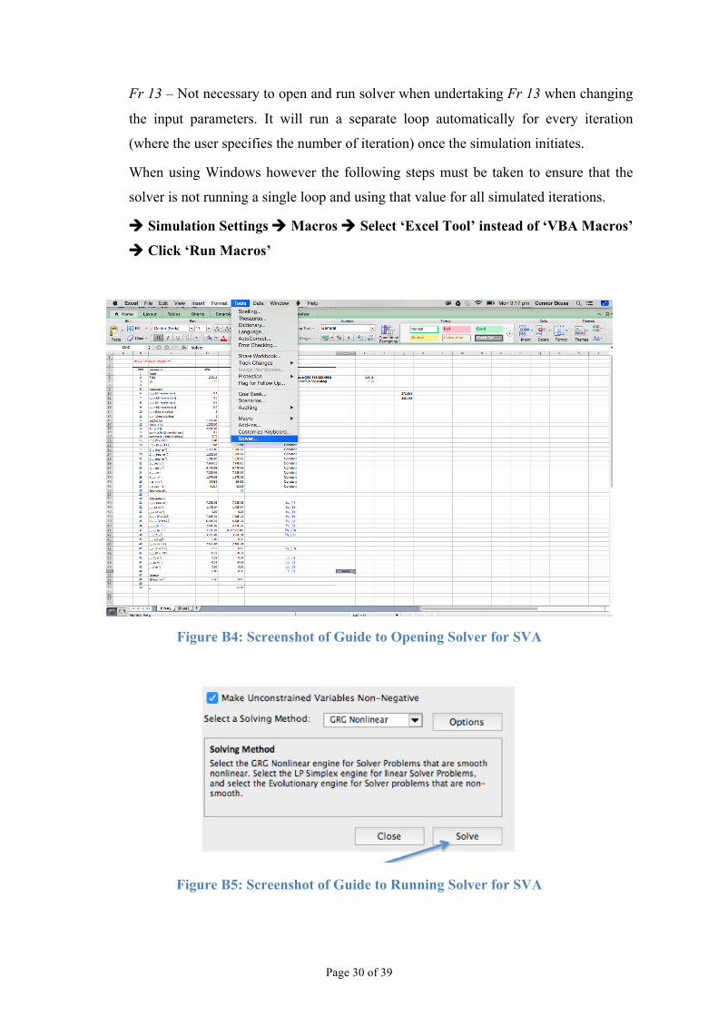
Page 30 of 39
Fr 13 – Not necessary to open and run solver when undertaking Fr 13 when changing
the input parameters. It will run a separate loop automatically for every iteration
(where the user specifies the number of iteration) once the simulation initiates.
When using Windows however the following steps must be taken to ensure that the
solver is not running a single loop and using that value for all simulated iterations.
à Simulation Settings à Macros à Select ‘Excel Tool’ instead of ‘VBA Macros’
à Click ‘Run Macros’
Figure B4: Screenshot of Guide to Opening Solver for SVA
Figure B5: Screenshot of Guide to Running Solver for SVA

Page 31 of 39
APPENDIX C
Table C1 – SVA and Fr 13 Results (T = 293.15 K, pH =5.15, Tolerance = 0 %)
Row Parameter SVA Fr 13 Simulation 1 Input 2 T (K) 293.15 293.15
RiskNormal(303.15,30.3,RiskTruncate(272.84,333.46))
3 pH 5.15 5.15 RiskNormal(5.15,0.515,RiskTruncate(4.635,5.
665)) 4 5 Constants 6 αa,Fe (dimensionless) 0.4 0.4 Constant 7 αa,H+ (dimensionless) 0.6 0.6 Constant 8 αc,Fe (dimensionless) 0.6 0.6 Constant 9 αc,H+ (dimensionless) 0.4 0.4 Constant
10 nFe (dimensionless) 2 2 Constant 11 nH+ (dimensionless) 1 1 Constant 12 e(0,Fe) (A) 1.00E-07 1.00E-07 Constant 13 e(0,H+) (A) 1.00E-07 1.00E-07 Constant 14 A,E (m^2) 2.83E-03 2.83E-03 Constant 15 𝛾,Fe (dimensionless) 0.3 0.3 Constant 16 𝛾,H+ (dimensionless) 0.75 0.75 Constant 17 E°Fe (V vs SCE) -0.681 -0.681 Constant 18 E°H+ (V vs SCE) -0.241 -0.241 Constant 19 Cs,Fe (mol m-3) 1.00E-03 1.00E-03 Constant 20 Cs,H+ (mol m-3) 1.00E-07 1.00E-07 Constant 21 Cb,Fe (mol m-3) 1.01E-05 1.01E-05 Constant 22 DFe (m2 s-1) 7.98E-10 7.98E-10 Constant 23 DH+ (m2 s-1) 9.47E-09 9.47E-09 Constant 24 δN,Fe (m2) 7.23E-06 7.23E-06 Constant 25 δN,H+ (m2) 1.67E-05 1.67E-05 Constant 26 F (C mol-1) 96485 96485 Constant 27 R (J mol-1 K-1) 8.314 8.314 Constant 28 Tolerance (%) - 0 29 30 Calculations 31 Cb,H+ (mol m3) 7.08E-03 7.08E-03 Eq. [1] 32 j0,Fe (A m-2) 1.40E-04 1.40E-04 Eq. [5] 33 j0,H+ (A m-2) 0.00 0.00 Eq. [7] 34 Erev,Fe (V vs SCE) -7.68E-01 -7.68E-01 Eq. [6] 35 Erev,H+ (V vs SCE) -6.48E-01 -6.48E-01 Eq. [4] 36 jmt,Fe (A m2) 2.11E-02 2.11E-02 Eq. [9]
37 jmt,H+ (A m2)
-3.87E-01 -
0.387335386
Eq. [10]
38 jct,Fe (A m2) 3.66E-01 3.66E-01 Eq. [11] 39 jct,H+(A m2) 0.00 0.00 40 ηFe (V vs SCE) 2.48E-01 2.48E-01 41 ηH+ (V vs SCE) 0.13 0.13 Eq. [13] 42 Ecorr (V vs. SCE) -0.52 -0.52 43 jFe (A m-2) 0.39 0.39 Eq. [6] 44 jH+ (A m-2) -0.39 -0.39 Eq. [6] 45 jT (A m-2) 0.00 0.00 Eq. [6] 46 0.00 0.00 Eq. [6] 47 Output 48 CR (mm yr-1) 0.45 0.45 49 50 p - 0.00 Eq. [16]
Page 32 of 39
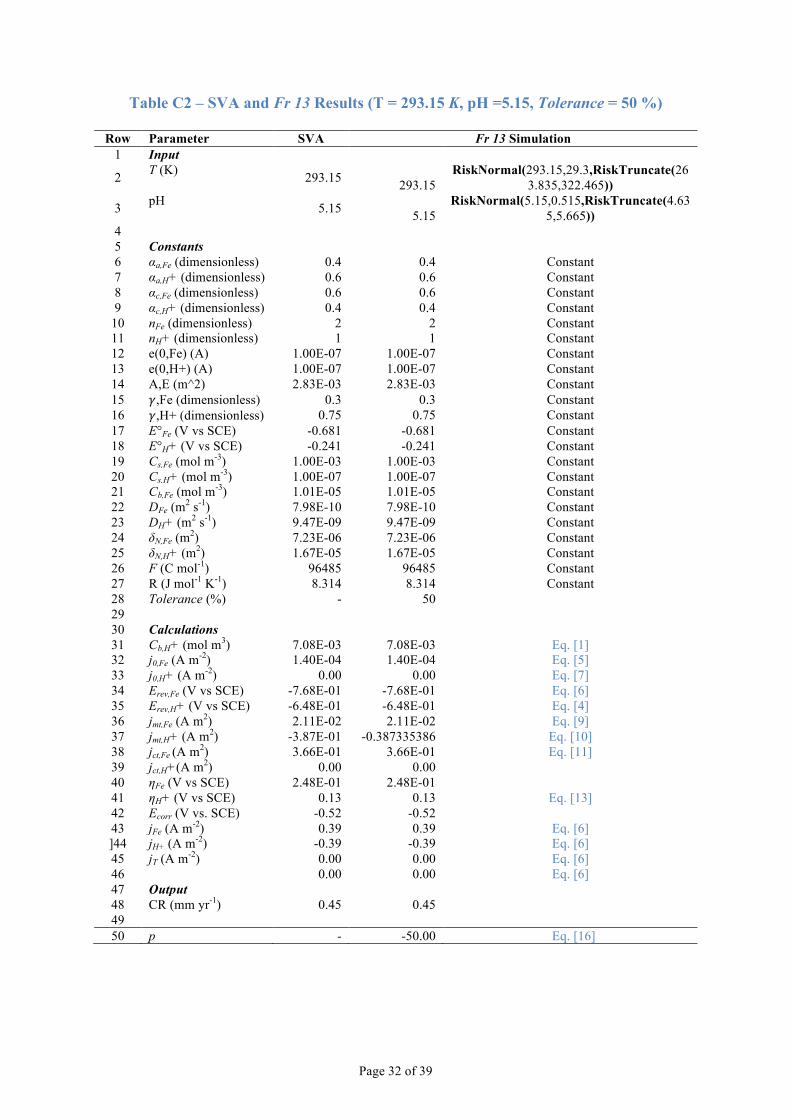
Table C2 – SVA and Fr 13 Results (T = 293.15 K, pH =5.15, Tolerance = 50 %)
Row Parameter SVA Fr 13 Simulation 1 Input 2 T (K) 293.15 293.15
RiskNormal(293.15,29.3,RiskTruncate(263.835,322.465))
3 pH 5.15 5.15 RiskNormal(5.15,0.515,RiskTruncate(4.63
5,5.665)) 4 5 Constants 6 αa,Fe (dimensionless) 0.4 0.4 Constant 7 αa,H+ (dimensionless) 0.6 0.6 Constant 8 αc,Fe (dimensionless) 0.6 0.6 Constant 9 αc,H+ (dimensionless) 0.4 0.4 Constant
10 nFe (dimensionless) 2 2 Constant 11 nH+ (dimensionless) 1 1 Constant 12 e(0,Fe) (A) 1.00E-07 1.00E-07 Constant 13 e(0,H+) (A) 1.00E-07 1.00E-07 Constant 14 A,E (m^2) 2.83E-03 2.83E-03 Constant 15 𝛾,Fe (dimensionless) 0.3 0.3 Constant 16 𝛾,H+ (dimensionless) 0.75 0.75 Constant 17 E°Fe (V vs SCE) -0.681 -0.681 Constant 18 E°H+ (V vs SCE) -0.241 -0.241 Constant 19 Cs,Fe (mol m-3) 1.00E-03 1.00E-03 Constant 20 Cs,H+ (mol m-3) 1.00E-07 1.00E-07 Constant 21 Cb,Fe (mol m-3) 1.01E-05 1.01E-05 Constant 22 DFe (m2 s-1) 7.98E-10 7.98E-10 Constant 23 DH+ (m2 s-1) 9.47E-09 9.47E-09 Constant 24 δN,Fe (m2) 7.23E-06 7.23E-06 Constant 25 δN,H+ (m2) 1.67E-05 1.67E-05 Constant 26 F (C mol-1) 96485 96485 Constant 27 R (J mol-1 K-1) 8.314 8.314 Constant 28 Tolerance (%) - 50 29 30 Calculations 31 Cb,H+ (mol m3) 7.08E-03 7.08E-03 Eq. [1] 32 j0,Fe (A m-2) 1.40E-04 1.40E-04 Eq. [5] 33 j0,H+ (A m-2) 0.00 0.00 Eq. [7] 34 Erev,Fe (V vs SCE) -7.68E-01 -7.68E-01 Eq. [6] 35 Erev,H+ (V vs SCE) -6.48E-01 -6.48E-01 Eq. [4] 36 jmt,Fe (A m2) 2.11E-02 2.11E-02 Eq. [9] 37 jmt,H+ (A m2) -3.87E-01 -0.387335386 Eq. [10] 38 jct,Fe (A m2) 3.66E-01 3.66E-01 Eq. [11] 39 jct,H+(A m2) 0.00 0.00 40 ηFe (V vs SCE) 2.48E-01 2.48E-01 41 ηH+ (V vs SCE) 0.13 0.13 Eq. [13] 42 Ecorr (V vs. SCE) -0.52 -0.52 43 jFe (A m-2) 0.39 0.39 Eq. [6] ]44 jH+ (A m-2) -0.39 -0.39 Eq. [6] 45 jT (A m-2) 0.00 0.00 Eq. [6] 46 0.00 0.00 Eq. [6] 47 Output 48 CR (mm yr-1) 0.45 0.45 49 50 p - -50.00 Eq. [16]
Page 33 of 39
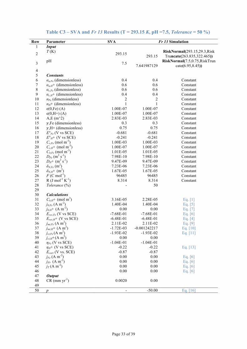
Table C3 – SVA and Fr 13 Results (T = 293.15 K, pH =7.5, Tolerance = 50 %)
Row Parameter SVA Fr 13 Simulation 1 Input 2 T (K) 293.15 293.15
RiskNormal(293.15,29.3,RiskTruncate(263.835,322.465))
3 pH 7.5 7.641987129 RiskNormal(7.5,0.75,RiskTrun
cate(6.95,8.45)) 4 5 Constants 6 αa,Fe (dimensionless) 0.4 0.4 Constant 7 αa,H+ (dimensionless) 0.6 0.6 Constant 8 αc,Fe (dimensionless) 0.6 0.6 Constant 9 αc,H+ (dimensionless) 0.4 0.4 Constant
10 nFe (dimensionless) 2 2 Constant 11 nH+ (dimensionless) 1 1 Constant 12 e(0,Fe) (A) 1.00E-07 1.00E-07 Constant 13 e(0,H+) (A) 1.00E-07 1.00E-07 Constant 14 A,E (m^2) 2.83E-03 2.83E-03 Constant 15 𝛾,Fe (dimensionless) 0.3 0.3 Constant 16 𝛾,H+ (dimensionless) 0.75 0.75 Constant 17 E°Fe (V vs SCE) -0.681 -0.681 Constant 18 E°H+ (V vs SCE) -0.241 -0.241 Constant 19 Cs,Fe (mol m-3) 1.00E-03 1.00E-03 Constant 20 Cs,H+ (mol m-3) 1.00E-07 1.00E-07 Constant 21 Cb,Fe (mol m-3) 1.01E-05 1.01E-05 Constant 22 DFe (m2 s-1) 7.98E-10 7.98E-10 Constant 23 DH+ (m2 s-1) 9.47E-09 9.47E-09 Constant 24 δN,Fe (m2) 7.23E-06 7.23E-06 Constant 25 δN,H+ (m2) 1.67E-05 1.67E-05 Constant 26 F (C mol-1) 96485 96485 Constant 27 R (J mol-1 K-1) 8.314 8.314 Constant 28 Tolerance (%) - 50 29 30 Calculations 31 Cb,H+ (mol m3) 3.16E-05 2.28E-05 Eq. [1] 32 j0,Fe (A m-2) 1.40E-04 1.40E-04 Eq. [5] 33 j0,H+ (A m-2) 0.00 0.00 Eq. [7] 34 Erev,Fe (V vs SCE) -7.68E-01 -7.68E-01 Eq. [6] 35 Erev,H+ (V vs SCE) -6.48E-01 -6.48E-01 Eq. [4] 36 jmt,Fe (A m2) 2.11E-02 2.11E-02 Eq. [9] 37 jmt,H+ (A m2) -1.72E-03 -0.001242217 Eq. [10] 38 jct,Fe (A m2) -1.93E-02 -1.93E-02 Eq. [11] 39 jct,H+(A m2) 0.00 0.00 40 ηFe (V vs SCE) -1.04E-01 -1.04E-01 41 ηH+ (V vs SCE) -0.22 -0.22 Eq. [13] 42 Ecorr (V vs. SCE) -0.87 -0.87 43 jFe (A m-2) 0.00 0.00 Eq. [6] 44 jH+ (A m-2) 0.00 0.00 Eq. [6] 45 jT (A m-2) 0.00 0.00 Eq. [6] 46 0.00 0.00 Eq. [6] 47 Output 48 CR (mm yr-1) 0.0020 0.00 49 50 p - -50.00 Eq. [16]

Page 34 of 39
Table C4 – SVA and Fr 13 Results (T = 293.15 K, pH =7.5, Tolerance = 0 %)
Row Parameter SVA Fr 13 Simulation 1 Input 2 T (K) 293.15 293.15
RiskNormal(293.15,29.3,RiskTruncate(263.835,322.465))
3 pH 7.5 7.641987129 RiskNormal(7.5,0.75,RiskTruncate(6.95,8.45)) 4 5 Constants 6 αa,Fe (dimensionless) 0.4 0.4 Constant 7 αa,H+ (dimensionless) 0.6 0.6 Constant 8 αc,Fe (dimensionless) 0.6 0.6 Constant 9 αc,H+ (dimensionless) 0.4 0.4 Constant
10 nFe (dimensionless) 2 2 Constant 11 nH+ (dimensionless) 1 1 Constant 12 e(0,Fe) (A) 1.00E-07 1.00E-07 Constant 13 e(0,H+) (A) 1.00E-07 1.00E-07 Constant 14 A,E (m^2) 2.83E-03 2.83E-03 Constant 15 𝛾,Fe (dimensionless) 0.3 0.3 Constant 16 𝛾,H+ (dimensionless) 0.75 0.75 Constant 17 E°Fe (V vs SCE) -0.681 -0.681 Constant 18 E°H+ (V vs SCE) -0.241 -0.241 Constant 19 Cs,Fe (mol m-3) 1.00E-03 1.00E-03 Constant 20 Cs,H+ (mol m-3) 1.00E-07 1.00E-07 Constant 21 Cb,Fe (mol m-3) 1.01E-05 1.01E-05 Constant 22 DFe (m2 s-1) 7.98E-10 7.98E-10 Constant 23 DH+ (m2 s-1) 9.47E-09 9.47E-09 Constant 24 δN,Fe (m2) 7.23E-06 7.23E-06 Constant 25 δN,H+ (m2) 1.67E-05 1.67E-05 Constant 26 F (C mol-1) 96485 96485 Constant 27 R (J mol-1 K-1) 8.314 8.314 Constant 28 Tolerance (%) - 0 29 30 Calculations 31 Cb,H+ (mol m3) 3.16E-05 2.28E-05 Eq. [1] 32 j0,Fe (A m-2) 1.40E-04 1.40E-04 Eq. [5] 33 j0,H+ (A m-2) 0.00 0.00 Eq. [7]
34 Erev,Fe (V vs SCE) -7.68E-01 -7.68E-01 Eq. [6]
35 Erev,H+ (V vs SCE) -6.48E-01 -6.48E-01 Eq. [4]
36 jmt,Fe (A m2) 2.11E-02 2.11E-02 Eq. [9]
37 jmt,H+ (A m2) -1.72E-03 -0.001242217 Eq. [10]
38 jct,Fe (A m2) -1.93E-02 -1.93E-02 Eq. [11]
39 jct,H+(A m2) 0.00 0.00 40 ηFe (V vs SCE) -1.04E-
01 -1.04E-01 41 ηH+ (V vs SCE) -0.22 -0.22 Eq. [13] 42 Ecorr (V vs. SCE) -0.87 -0.87 43 jFe (A m-2) 0.00 0.00 Eq. [6] 44 jH+ (A m-2) 0.00 0.00 Eq. [6] 45 jT (A m-2) 0.00 0.00 Eq. [6] 46 0.00 0.00 Eq. [6] 47 Output 48 CR (mm yr-1) 0.0020 0.00 49 50 p - 0.00 Eq. [16]

Page 35 of 39
Table C5 – SVA and Fr 13 Results (T = 293.15 K, pH =3.0, Tolerance = 50 %)
Row Parameter SVA Fr 13 Simulation 1 Input 2 T (K) 293.15 293.15
RiskNormal(293.15,29.3,RiskTruncate(263.835,322.465))
3 pH 3 3 RiskNormal(3,0.3,RiskTruncate(2.7,3.3)) 4 5 Constants 6 αa,Fe (dimensionless) 0.4 0.4 Constant 7 αa,H+ (dimensionless) 0.6 0.6 Constant 8 αc,Fe (dimensionless) 0.6 0.6 Constant 9 αc,H+ (dimensionless) 0.4 0.4 Constant
10 nFe (dimensionless) 2 2 Constant 11 nH+ (dimensionless) 1 1 Constant 12 e(0,Fe) (A) 1.00E-07 1.00E-07 Constant 13 e(0,H+) (A) 1.00E-07 1.00E-07 Constant 14 A,E (m^2) 2.83E-03 2.83E-03 Constant 15 𝛾,Fe (dimensionless) 0.3 0.3 Constant 16 𝛾,H+ (dimensionless) 0.75 0.75 Constant 17 E°Fe (V vs SCE) -0.681 -0.681 Constant 18 E°H+ (V vs SCE) -0.241 -0.241 Constant 19 Cs,Fe (mol m-3) 1.00E-03 1.00E-03 Constant 20 Cs,H+ (mol m-3) 1.00E-07 1.00E-07 Constant 21 Cb,Fe (mol m-3) 1.01E-05 1.01E-05 Constant 22 DFe (m2 s-1) 7.98E-10 7.98E-10 Constant 23 DH+ (m2 s-1) 9.47E-09 9.47E-09 Constant 24 δN,Fe (m2) 7.23E-06 7.23E-06 Constant 25 δN,H+ (m2) 1.67E-05 1.67E-05 Constant 26 F (C mol-1) 96485 96485 Constant 27 R (J mol-1 K-1) 8.314 8.314 Constant 28 Tolerance (%) - 50 29 30 Calculations 31 Cb,H+ (mol m3) 1.00E+0
0 1.00E+00 Eq. [1]
32 j0,Fe (A m-2) 1.40E-04 1.40E-04 Eq. [5] 33 j0,H+ (A m-2) 0.00 0.00 Eq. [7]
34 Erev,Fe (V vs SCE) -7.68E-01 -7.68E-01 Eq. [6]
35 Erev,H+ (V vs SCE) -6.48E-01 -6.48E-01 Eq. [4]
36 jmt,Fe (A m2) 2.11E-02 2.11E-02 Eq. [9]
37 jmt,H+ (A m2) -
5.47E+01
-54.71334483 Eq. [10]
38 jct,Fe (A m2) 1.63E+01 1.63E+01 Eq. [11]
39 jct,H+(A m2) 0.00 0.00 40 ηFe (V vs SCE) 3.68E-01 3.68E-01 41 ηH+ (V vs SCE) 0.25 0.25 Eq. [13] 42 Ecorr (V vs. SCE) -0.40 -0.40 43 jFe (A m-2) 16.27 16.27 Eq. [6] 44 jH+ (A m-2) -54.71 -54.71 Eq. [6] 45 jT (A m-2) -38.44 -38.44 Eq. [6] 46 38.44 38.44 Eq. [6] 47 Output 48 CR (mm yr-1) 18.79 18.79 49 50 p - -50.00 Eq. [16]

Page 36 of 39
Table C6 – SVA and Fr 13 Results (T = 293.15 K, pH =3.0, Tolerance = 50 %)
Row Parameter SVA Fr 13 Simulation 1 Input 2 T (K) 293.15 293.15
RiskNormal(293.15,29.3,RiskTruncate(263.835,322.465))
3 pH 3 3 RiskNormal(3,0.3,RiskTruncate(2.7,3.3)) 4 5 Constants 6 αa,Fe (dimensionless) 0.4 0.4 Constant 7 αa,H+ (dimensionless) 0.6 0.6 Constant 8 αc,Fe (dimensionless) 0.6 0.6 Constant 9 αc,H+ (dimensionless) 0.4 0.4 Constant
10 nFe (dimensionless) 2 2 Constant 11 nH+ (dimensionless) 1 1 Constant 12 e(0,Fe) (A) 1.00E-07 1.00E-07 Constant 13 e(0,H+) (A) 1.00E-07 1.00E-07 Constant 14 A,E (m^2) 2.83E-03 2.83E-03 Constant 15 𝛾,Fe (dimensionless) 0.3 0.3 Constant 16 𝛾,H+ (dimensionless) 0.75 0.75 Constant 17 E°Fe (V vs SCE) -0.681 -0.681 Constant 18 E°H+ (V vs SCE) -0.241 -0.241 Constant 19 Cs,Fe (mol m-3) 1.00E-03 1.00E-03 Constant 20 Cs,H+ (mol m-3) 1.00E-07 1.00E-07 Constant 21 Cb,Fe (mol m-3) 1.01E-05 1.01E-05 Constant 22 DFe (m2 s-1) 7.98E-10 7.98E-10 Constant 23 DH+ (m2 s-1) 9.47E-09 9.47E-09 Constant 24 δN,Fe (m2) 7.23E-06 7.23E-06 Constant 25 δN,H+ (m2) 1.67E-05 1.67E-05 Constant 26 F (C mol-1) 96485 96485 Constant 27 R (J mol-1 K-1) 8.314 8.314 Constant 28 Tolerance (%) - 0 29 30 Calculations 31 Cb,H+ (mol m3) 1.00E+00 1.00E+00 Eq. [1] 32 j0,Fe (A m-2) 1.40E-04 1.40E-04 Eq. [5] 33 j0,H+ (A m-2) 0.00 0.00 Eq. [7] 34 Erev,Fe (V vs SCE) -7.68E-01 -7.68E-01 Eq. [6] 35 Erev,H+ (V vs SCE) -6.48E-01 -6.48E-01 Eq. [4] 36 jmt,Fe (A m2) 2.11E-02 2.11E-02 Eq. [9] 37 jmt,H+ (A m2) -5.47E+01 -54.71334483 Eq. [10] 38 jct,Fe (A m2) 1.63E+01 1.63E+01 Eq. [11] 39 jct,H+(A m2) 0.00 0.00 40 ηFe (V vs SCE) 3.68E-01 3.68E-01 41 ηH+ (V vs SCE) 0.25 0.25 Eq. [13] 42 Ecorr (V vs. SCE) -0.40 -0.40 43 jFe (A m-2) 16.27 16.27 Eq. [6] 44 jH+ (A m-2) -54.71 -54.71 Eq. [6] 45 jT (A m-2) -38.44 -38.44 Eq. [6] 46 38.44 38.44 Eq. [6] 47 Output 48 CR (mm yr-1) 18.79 18.79 49 50 p - 0.00 Eq. [16]

Page 37 of 39
Fig. C1: r-MC Risk Factor Distribution (T = 293.15 K, pH =5.15, Tolerance = 0 %)
Fig. C2: r-MC Risk Factor Distribution (T = 293.15 K, pH =5.15, Tolerance = 50 %)

Page 38 of 39
Fig. C3: r-MC Risk Factor Distribution (T = 293.15 K, pH =3, Tolerance = 0 %)
Fig. C4: r-MC Risk Factor Distribution (T = 293.15 K, pH =3, Tolerance = 50 %)

Page 39 of 39
Fig. C5: r-MC Risk Factor Distribution (T = 293.15 K, pH =7.5, Tolerance = 0 %)
Fig. C6: r-MC Risk Factor Distribution (T = 293.15 K, pH =7.5, Tolerance = 50 %)