understanding economic effects of spatial investments
TRANSCRIPT
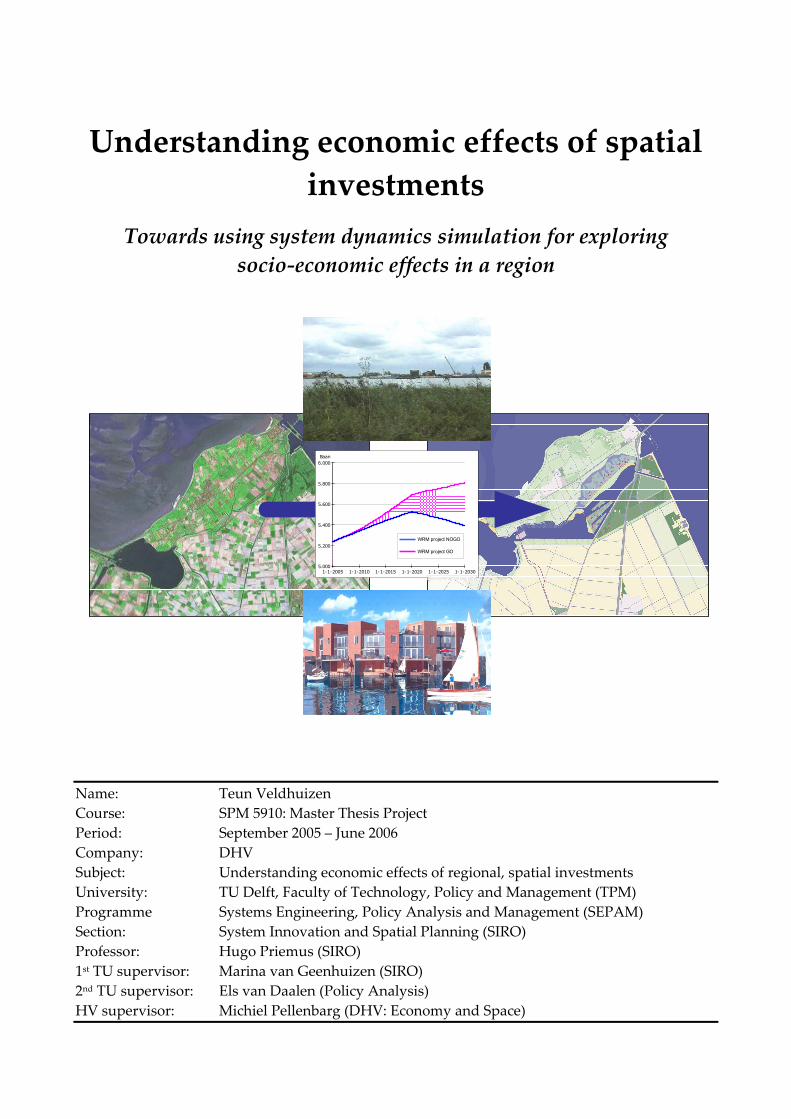
Understanding economic effects of spatial
investments
Towards using system dynamics simulation for exploring
socio-economic effects in a region
Name: Teun Veldhuizen
Course: SPM 5910: Master Thesis Project
Period: September 2005 – June 2006
Company: DHV
Subject: Understanding economic effects of regional, spatial investments
University: TU Delft, Faculty of Technology, Policy and Management (TPM)
Programme Systems Engineering, Policy Analysis and Management (SEPAM)
Section: System Innovation and Spatial Planning (SIRO)
Professor: Hugo Priemus (SIRO)
1st TU supervisor: Marina van Geenhuizen (SIRO)
2nd TU supervisor: Els van Daalen (Policy Analysis)
HV supervisor: Michiel Pellenbarg (DHV: Economy and Space)
1-1-2005 1-1-2010 1-1-2015 1-1-2020 1-1-2025 1-1-20305.000
5.200
5.400
5.600
5.800
6.000
Baan
Non-commercial use only!
WRM project NOGO
WRM project GO

- 2 -

-I -
Preface
This thesis has been written in the scope of the completion of the Systems Engineering, Policy
Analysis and Management master at the faculty of Technology, Policy and Management at Delft
Technical University. The research has been facilitated by the department of Consultancy:
Economy and Space from DHV.
After first having talked to Michiel Pellenbarg from DHV in midsummer of 2005 I immediately
was enthusiastic about his idea of creating an instrument, able to support policy makers in making
better decisions. My mind started working overtime and before I knew it a research proposal took
shape and found its way to Marina van Geenhuizen, Els van Daalen and Hugo Priemus. A
question that was pertinent from the start was why no one had studied my idea and why such an
instrument did not exist. That question chased me trough the thesis project and functioned as a
research driver.
I would like to thank Michiel Pellenbarg for supporting me in a great manner. Time has flown by it
seems. I would also like to thank Els van Daalen for controlling the scope of this project and
Marina van Geenhuizen for the long regional economic discussions. The last member of the thesis
team is Hugo Priemus whom I thank for his talent to point out the core of a problem in one
sentence.
Bedankt!
Teun

- II -

-III -
Summary
Seeing into the future remains until today a subject for philosophers and science fictions novels.
Non-the-less, countless efforts are made today that aim at predicting economic developments,
stock level prices and other future events (respectively the CPB1, financial organizations and
evangelists). These predictions all provide a footing for making decisions in the present that will
have effects in the future. When making decisions on large spatial investments, an analysis of the
effects of the investment is important for both governmental and private organisations. A broad
range of methods exists that allow a glance of the future. A sketch or drawing can provide a policy
maker with the effects the investment will have on the landscape. A traffic model indicates the
expected traffic volume and welfare effects can be assessed with the Social Cost Benefit Analysis
(Eijgenraam et al. 2000). However, there seems to be no instrument available for analysis of socio-
economic effects of spatial investments on a municipal scale. And the demand for such an
instrument is rising. Currently available models that describe socio-economic effects have either a
wrong geographical focus, are only focussed on infrastructure or are unable to deal with economic
dynamics. Furthermore, none of these instruments facilitates communication between the
consultant (the model developer) and the policy maker (the decision maker). This is a shame,
according to the former head of the CPB Henk Don (2004), both parties can learn from each other
in an effort to make better spatial investment decisions. Therefore, the instrument should have an
open and communicable structure.
A methodology that can be used for the development of an instrument that satisfies the demands
mentioned above is system dynamics (Forrester 1958). System dynamic (SD) models tend to be
small and comprehensible, hence relatively easy to understand. Furthermore they correspond with
the feeling that real systems are non-linear, multivariable, time-delayed and disaggregate
(Meadows 1976). System dynamics enables learning and makes it also possible to explore possible
scenarios and potential policy options (Spector 2000). Combined with a strong visual presentation
of causal relations SD makes an ideal method to facilitate communication of socio-economic
effects. The question becomes then, to what extend SD can contribute to the ex-ante exploration
and assessment of policy options in spatial investments in a region?
To answer this question a system dynamics model is developed that forecasts socio-economic
effects on a municipal scale. For a start more research in existing spatial models is executed (van
Oort, et al. 2005). This research leads to the conclusion that a lot of concepts of existing models can
be used in the “thesis model”. For instance the way in which shift-share analysis is used in the
REGINA model (Koops 2005). The second step in the development of the “thesis model” is to
acquire the requirements for the model. For this purpose consultants and policy makers have been
interviewed as respondents in a requirement analysis. The result are that the model must be able
to:
• export the data from the instrument to excel for further processing and storage of output data.
• have an interface that includes both a simple (“Jip & Janneke”) and a complex presentation of
model outcomes.
• include forecasts for regional demography, employment, housing market and gross regional
product.
1 CPB: the Netherlands Bureau for Economic Policy Analysis

- IV -
• show a distribution of the uncertainty of the outcomes and the sensitivity of the input
parameters.
• show effects of different policy options under different economic scenarios.
Based on the list of the requirements, the SD methodology and the literature research a concept
model is developed that includes all the important socio-economic variables. The concept model is
then translated into a simulation model in the PowerSim Studio 2005 (SD) software package.
PowerSim has excellent visual capabilities, supports the design of an interface and has sensitivity
analysis functions. Because one of the basic properties of SD is that the model must be kept as
simple as possible the regional demographic development is not included in the concept model. In
stead the time series outcomes of the PRIMOS2 model are used and fed directly into the simulation
model (Heida 2002). This reduces the size and complexity of the model notably. Furthermore, as
explanatory factor for the development of jobs in the region the theorem that jobs-follow-people is
used (Vermeulen & van Ommeren 2005, 2006). This means that the development of dwellings in a
region is a leading indicator of the growth of jobs. In order to comply with the requirement that the
model must be able to present results in a “Jip & Janneke” style and more complex the user
interface of the model has been designed. The final simulation model has over 85% of the
requirements implemented, including the most important requirements mentioned in the list
above. An example of a requirement that is not implemented is the demand that the simulation
model must be able to cope with effects on a provincial scale. This would require more complex
variables and relations like province competitiveness and inter regional trade. The geographical
focus of the simulation model remains a (multi) municipal scale with at least 20.000 inhabitants.
The simulation model is tested on applicability using historic data validation, group testing
sessions and expert interviews. The interviews include several spatial modelling experts3 whose
ideas contributed a great deal in the coming about of the thesis model. All experts concluded that
they had never witnessed a model with an adaptable interface that allows the user to change input
parameters and calculate the outcomes real-time. The group sessions illustrated that the
instrument can work very effectively as a communication tool. This success can be attributed to the
facts that questions concerning the socio-economic effects can be calculated and answered right
away.
There are some points of attention that should be regarded when using the thesis model. The CPB
scenarios that are used to forecast the economic growth have a large influence on the outcomes of
the simulation model. The contrast between an optimistic or pessimistic scenario can change the
final investment decision as the difference for jobs for instance rises up to 20%. However, sensible
use of economic scenarios can also improve the investment decision. The value of the prediction
made by the model is tested by an historic validation. The model proved to have an average
deviation from the actual regional jobs of 4,4%4. This is regarded as acceptable for the use of the
instrument as socio-economic effect exploration instrument. Based on the sensitivity analysis and
historic validation and excluding the effect of different CPB scenarios the uncertainty bound of the
model outcomes is 10%. This should be kept in mind when working with these outcomes.
2 PRIMOS is a demographic forecast model which makes forecasts for all the Dutch municipalities. 3 The expert interviews included spatial model experts F. van Oort, M. Thissen and W. Vermeulen. 4 Based on time series: 1998-2005. Historic PRIMOS and CBS data is used and the historic industry sector
performance is calculated with regression analysis based on data from 1993-1998.

-V -
The simulation model is developed with the aim to apply the model in different projects, hence for
different regions. This is made physically possible through the loosely coupled relation between
the input variables in an Excel database and the simulation model in PowerSim. Furthermore the
model is built in components that can be adapted to fit effects of different regions. The simulation
model is therefore physically capable of dealing with different project regions. As mentioned
above the municipal level binds the geographical scale of the model. Differences that exist between
urban and rural regions do not present a problem for the simulation model (Interview Vermeulen).
However regions with extensive industries and high concentrations of jobs have more complex
economic relations. Unless these relations are built into the model it should not be used for
industry intensive regions.
The verdict on the simulation model is that it can be used for the assessment and exploration of
socio-economic effects. The question remains what the added value of system dynamics is? First
the causal thinking (inherent to SD) relates closely to mental models, which makes discussions of
the relations in the model relatively simple. This simplicity is desired for the communication
between policy makers and consultants. Therefore the most important principle when using a SD
methodology is to make sure that the policy maker understands the consequences of a proposed
policy option. This will assist policy makers in understanding the non-linear developments in a
project region. The elaborate visual representations of the outcomes of the simulation model also
contribute to a better understanding of the economic system by the policy maker (Forrester 1980).
It also provides a platform on which the consultant (assisting the policy maker) and the policy
maker can discuss potential situations in the project region. This in turn involves the consultant
more in the local issue, giving him or her a more profound basis on which to form
recommendations.

- VI -
Table of contents
Preface _______________________________________________________________________________ I
Summary ____________________________________________________________________________III
Table of contents ______________________________________________________________________ VI
1 Research project setup_______________________________________________________________ 1
1.1 Introduction __________________________________________________________________ 1
1.2 Research questions____________________________________________________________ 4
1.3 Research framework___________________________________________________________ 6
1.4 Introduction of case study: Wieringerrandmeer__________________________________ 10
2 Model conditions and environment____________________________________________________ 17
2.1 Policy making and simulation models__________________________________________ 17
2.2 What are regional investment projects? _________________________________________ 20
2.3 Finding the model requirements_______________________________________________ 20
2.4 Existing spatial, regional economic models _____________________________________ 29
2.5 The potential of system dynamics______________________________________________ 36
2.6 Available data for model input variables _______________________________________ 41
2.7 Conclusion of model conditions and environment _______________________________ 42
3 Model construction ________________________________________________________________ 45
3.1 The simulation model concept_________________________________________________ 45
3.2 Cause-and-effect relationships as basis for the concept model_____________________ 48
3.3 Translation of the concept- into the simulation model____________________________ 56
3.4 Assumptions made during the development of the simulation model ______________ 66
3.5 User interface: communicating with policy makers and consultants________________ 70
3.6 Conclusions of the model construction _________________________________________ 73
4 Model validation and requirement testing ______________________________________________ 75
4.1 Steps in model validation _____________________________________________________ 75
4.2 Sensitivity analysis___________________________________________________________ 78
4.3 Applicability of the simulation model__________________________________________ 84
4.4 Performing group and expert tests _____________________________________________ 88
4.5 Conclusions of model validation and requirement testing ________________________ 92
5 Conclusions ______________________________________________________________________ 99
5.1 The thesis questions partly satisfied ___________________________________________ 99
5.2 The model in practice: socio-economic analysis of the WRM investment project____ 108
-VII -
6 Recommendations and reflection ____________________________________________________ 112
6.1 Recommendations for further research ________________________________________ 112
6.2 Learning experiences from developing the simulation model ____________________ 114
6.3 Limits of simulation model use _______________________________________________ 115
7 Literature _______________________________________________________________________ 117
8 Appendices ______________________________________________________________________ 122
8.1 Appendix 1: List of definitions and abbreviations ______________________________ 122
8.2 Appendix 2: preparation for the requirement analysis ___________________________ 123
8.3 Appendix 3: Questionnaires__________________________________________________ 125
8.4 Appendix 4: Lists of interviewees _____________________________________________ 129
8.5 Appendix 5: Policy maker questionnaire long list_______________________________ 130
8.6 Appendix 6: The final requirement lists _______________________________________ 138
8.7 Appendix 7: What is Shift and Share analysis __________________________________ 143
8.8 Appendix 8: How PowerSim deals with large data arrays ___________________________ 144
8.9 Appendix 9: Exploring the relation between PowerSim Studio and MS Excel ______ 145
8.10 Appendix 10: description of the group tests and expert validations _______________ 146


Understanding economic effects of spatial investments
-1 -
1 Research project setup
1.1 Introduction
Political decisions concerning large infrastructural and spatial projects cause a lot of controversy.
Not only because these decisions have far going consequences for the Dutch landscaped but also
because doubt exists to whether these projects are economically justifiable. The economic benefits
are – in some cases – very slim and vulnerable to scrutiny because the benefits do not hold in all
economic scenarios. Recent projects that are now under construction (e.g. the Betuwe lijn and the
HSL) have led to increased social and political discussions about the economic benefits of such
projects. In 2004 a temporary commission5 (TCI 2004) was appointed by the government to
research the causes of the budget overruns and delays in large infrastructure projects. Next to this
political development already in 2000 a directive was drawn up for the vindication of large
(infrastructure) projects. The directive stems from the Research program Economic Effect of
Infrastructure (OEI) and advocates a methodology that is called Social Cost Benefit Analysis
(SCBA) (Eijgenraam et al. 2000). The use of a SCBA is obligatory for large national projects,
however it is also deployed voluntary for projects on a smaller geographical scale6. SCBA helps
quantifying welfare costs and benefits and is aimed at preventing double counting of effects of an
investment project. Although the SCBA includes positive and negative welfare effects, it does not
illustrate the terms on which policy makers reach their intended policy goal.
Some conclusions of the TCI issued that even more care should be taken in quantifying risks early
in a project. They observed the systematic underestimation of the costs and overestimation of the
revenue on large infra structure projects (TCI 2004 pp. 15). To counter these effects more funded
arguments resulting from independent research have to be collected. Especially the early phases of
decision-making lack structure in coming to a clear judgement. Premature, unfunded prognoses
may not be allowed to influence the future decisions as these early projections are often biased and
based on speculation. These problems are not only present on a national scale; projects on a lower
geographical scale also require better assessment in early policy phases. The demand for these
regional effect studies has risen over the last year7. A problem that policy-supporting consultants
face is that the instruments for policy analysis at their disposal are either unsuited for smaller
projects (Vermeulen & van Ommeren 2005, 2006), only focused on infrastructure (Thissen 2005) or
unable deal with the economic dynamics (Blok, 2002). A possible solution to the problems
mentioned above could be an instrument in the shape of a simulation model that is able to support
policy makers in dealing with risks early in the policy process. Both consultants and policy makers
should be involved in the development of this instrument. In that line of thought Don (2004) writes
that policy makers and (model developing) consultants should work more closely together in
order to learn from each other. The policy makers are often not aware of the underlying model
assumptions where they often should be in order to put their policy proposal in perspective. Don
too, established the lack of risk assessment in large, complex projects and thinks that econometric
models can assist policy makers in pointing out the high risk factors in their policy proposals.
5 Tijdelijke Commissie Infrastructuurprojecten (TCI) 6 From the website of Ecorys: visited on 29-03-2006: http://www.ecorys.nl/projecten/vv_infra_p1.php 7 An increase in tenders was noticed by employees of DHV Economy and Space (June – September 2005)

Master Thesis – Teun Veldhuizen
- 2 -
Currently available economic models for regional economic projections are either too complex or
not suited for the assessment of municipalities. Therefore an instrument needs to be developed
that has an accessible structure, this way the model becomes an instrument that is able to illustrate
how economic results come about. This does not mean that the existing models cannot assist in the
coming about of the thesis model. The thesis model should facilitate the collaboration between
policy makers and consultants and enable smoother knowledge exchange. Furthermore, the model
should support policy makers in dealing with uncertainties that are present early in the policy
process.
1.1.1 Research issue: assessing system dynamics applications in spatial problems
Last year the engineers of DHV Economy and Space (E&S) observed an increase in the demand
from local governments for long-term regional investment effect studies. In these studies an
assessment is conducted of the economic effects of an investment on regional scale. Such an
investment can be infrastructure development, a city extension plan or area redevelopment. This
increasing demand can be attributed to two major developments. First the introduction of the dual
system directive in March 2002: in the dual system the municipal tasks have been divided more
clearly. Members of the municipal council have a larger monitoring responsibility toward the city
administrators. The administrators have to justify investment plans and need support in the form
of an effect analysis or forecast. A second and perhaps more significant development is the gradual
shift from admission planning towards development planning8. Roughly put, development
planning allows ideas for regional development to come from the municipalities instead from the
central government. In this situation the municipality has to justify the proposed investment
towards the central government, an effect analysis or model can be a supportive tool in this matter
The current analytical methods that E&S have available are sufficient to supply their clients with
an economical forecast, however a standard model or modelling approach is not used. There are
models available on the market developed by other firms and institutions however these models
do not fulfil the specific needs of DHV E&S. Either the geographical scale is too high and lacks a
municipal scope, the model is too complex or the model is too costly to use. The SCBA is an
available technique; however the SCBA remains more a way of inventorying welfare effects than it
is an actual simulation model. Several models have been developed by both public organizations
as by private firms, like The RAEM model, developed by the Netherlands Institute for Spatial
Research (RPB). RAEM is a monopolistic competition model that is aimed at evaluating policy on
transport infrastructure (Thissen 2005). It does this however on a national scale; the results are
therefore focused on a national level of policy making, not on lower geographical scales.
Furthermore the RAEM model is extremely complex and would, even for a model expert, be hard
to comprehend and is not suited for interaction between consultant and policy maker.
A model that focuses more specifically on the municipal level is PRIMOS, developed by ABF
Research. It is designed to make forecasts on demographic developments in Dutch municipalities
until 2040 (Blok 2005; Heida 2002). The PRIMOS model could not be used for the early assessment
of projects because it does not include socio-economic effects. Several other models use the time
series data output of PRIMOS as input data hereby omitting a demographic model component. A
model that is able to calculate economic effects on a municipal level is REGINA. The REGINA
8 From brochure of the Rathenau institute, Habiforum and NIROV: Ontwikkelingsplanologie als social-culturele opgave
(2004)

Understanding economic effects of spatial investments
-3 -
model is developed by the Netherlands Organization for Applied Scientific Research (TNO) and is
aimed at providing regional employment and industry growth projections. Compared to the
RAEM and PRIMOS model, the REGINA model is relatively easy to comprehend (Koops 2005).
The primary function however, remains identifying differences in economic growth between
regions or municipalities, not the ex-ante calculation of regional investments. These currently
available models can be considered complex black-box systems that can only be used by model
experts. This leads to a situation where only the model expert is aware of why the model behaves
as it does; while in fact it is important to convey this knowledge to the policy maker in order to let
them make better decisions (Don, 2004). The models that are discussed all lack the ability to be able
to be used in situations where the policy maker and consultant together can come to solutions. To
sum up, there are four issues why the currently available models do not suffice:
1. The geographical scale is too high, not on a municipal level
2. The models do not sufficiently deal with uncertainties
3. The models are too complex
4. Policy makers are not aware of the underlying model assumptions
The four issues mentioned above and the demand for an instrument that can quantify and
communicate socio-economic effects in region lead to the use of system dynamics. System
dynamics provides insight for policy makers in regional investment decisions based on causal
relations. SD has certain advantages; it relates closely to “mental models” that people perceive in a
problem (Forrester 1958, 1969) and is therefore easy to communicate. Furthermore SD is an
approach that is used for general understanding of a problem and SD models tend to be small and
comprehensible, hence relatively easy to understand. System dynamics transforms these mental
models into causal relationship diagrams indicating directionality and nature of the effect. It
corresponds with the feeling that real systems are non-linear, multivariable, time-delayed and
disaggregate (Meadows 1976). Most people are capable of logically deducting these causal
relationships between two factors and so creating a visual model from their mental model. System
dynamics enables learning and makes it also possible to perform explorations of possible scenarios
and policy options (Spector 2000). This enables a consultant, supporting a policy maker to involve
him or her in the socio-economic processes that take part in “their” project region. With a
visualized model, feedback loops can be identified that would have been obscured in a mental
model due to the complexity and non-linearity of the real-life system. The ability of transforming
complex, mental models into tangible and quantifiable models is a great strength of the system
dynamics approach.
An effort to model the dynamics of a growing city has been undertaken by Forrester (1969) with
his Urban Dynamics (UD) model. This model simulated a small rural community that grows up to
be a medium sized town. The model incorporates different types of housing, work and industries.
This UD model functions as a starting point for the development of this thesis model. This means
that the thesis model will not be focused on infrastructure development but on housing projects,
regional facilities and the expansion of business parks.
1.1.2 Research objective
The general objective of this master thesis is threefold. The first objective is to plot a set of
demands that need to be fulfilled by the instrument. These demands consist of a scientific part and
a practical part. The scientific demands come from studying existing model and performing a

Master Thesis – Teun Veldhuizen
- 4 -
literature study. The second objective is to create (part of) this simulation model. The third and
final objective is to convey the knowledge gained during the completion of this thesis project
towards other people.
The simulation model is intended for use in regional policy processes meaning in and between
municipalities. More specifically the respective purpose of the simulation model is to support
policy makers in the process of developing alternative policy options and testing the consequences
of those options. The model can assist policy makers in attributing uncertainties and dealing with
them early in the policy process. In that sense the model can be called an instrument that is aimed
at strengthening the development of new policy.
1.2 Research questions
To overcome the problems mentioned above an approach will be explored in this thesis project
that has the potential to provide policy makers with an ex-ante assessment of the economic effects
of their policy options. The approach will aid in exploring questions concerning long-term
economic effects on a multi municipality geographical scale. The angle of approach that will be
used is called System Dynamics (SD). Using SD has several advantages; it relates closely to ‘mental
models’ that people perceive in a problem (Forrester 1980, Meadows 1976) and can therefore
directly be used in communication with the client. Furthermore SD is an approach that is used for
general understanding of a problem and tends to be small and comprehensible (Meadows, 1976),
meaning that SD models are transparent and relatively easy to understand. SD models express the
kind of dynamics that is also present in reality and that is impossible to express with linear
models. The goal of this SEPAM masters thesis is to develop – part of – a simulation model aided
by SD that assesses the long-term, socio-economic effects of regional investments. This model
should be able to make long-term forecasts, include multiple scenarios, first and second order
economic effects and estimations about the regions prosperity. The main research question
therefore is:
How can the system dynamics approach contribute to the ex-ante exploration and assessment of
policy options in spatial investments in a region?
Substantiating the main research question is a set of 3 sub questions that contribute to finding the
answer to the main question. The first sub question concerns the leading economic indicators and
their underlying relations have to be discovered. In order to find these indicators the user
requirement and existing regional economic model should be analyzed. Annotating that during
the search for the instrument requirements realism should be kept in mind. Interesting
requirements might surface that are impossible to implement for time or resource constraints.
Furthermore the requirements found through the analysis must not contradict; where
contradiction is established choices will need to be made whether to accept the one or the other. By
asking what can be learned from the existing regional economic instrument know issues can be
picked up in an early stage. Studying the existing models also leads to the question what data
sources are required for calculating the desired effects.

Understanding economic effects of spatial investments
-5 -
1) What are the leading indicators and underlying relations of an instrument for the ex-ante
exploration and assessment of policy options in spatial investments in a region?
a. What are the user requirements of such an instrument?
b. What can be learned and used from the existing models or instruments for regional economic
analysis?
c. What are the generally accepted data sources that can be used as input parameters for such
an instrument?
The second sub question concerns the construction of the simulation model. To come to the final
simulation model two translations have to be made. First the translation of the requirement
analysis, literature study and existing model study into a concept model. And second the
translation of the concept model into the final mathematical simulation model.
2) How to construct an instrument for the ex-ante exploration and assessment of policy options in
spatial investments in a region?
a. How are the notions from the requirement analysis, literature study and existing models
translated into a conceptual model?
b. How is this conceptual model translated into a mathematical simulation model?
The third sub question focuses on the applicability of the instrument once it is finished and tested.
How detailed is the information that can be extracted from the instrument and how accurate are
the forecasts? It also has to be seen if it has been possible to fit all the user requirements into the
final instrument. Furthermore the third sub question satisfies contemplation concerning the
applicability of the developed instrument on multiple regions and different geographical scale
levels. As economic differences exist, between for instance; a rural region and an urban region the
question is whether the instrument is applicable in different regions.
3) What is the practical applicability of the developed instrument?
a. What is the robustness of the model in terms of predictability?
b. Can the instrument fulfil the requirements that were initially set at the start of this
research?
c. Is the instrument applicable for regions with different characteristics?

Master Thesis – Teun Veldhuizen
- 6 -
1.3 Research framework
The research questions from the previous section form the basis for the research framework. The
research framework illustrates the methodology and strategies used in the coming about of this
thesis project. The framework assists in structuring the research tasks, it paves a path of steps that
have to be taken in order to complete the research (Verschuren 1999). The research is structured in
thirteen activities (steps) that have to be executed in order to answer the research questions.
Figure 1.1, the research framework
The “kick-off” of the project can be found in chapter 1 and comprises of the first three steps. First a
preliminary literature study assists in formulating the research questions. A case study will be
used throughout the project to illustrate the practical implications of choices that are made. The
next three steps try to answer the first sub question. In step 4 a requirement analysis is performed
to get a grip on the most important economic indicators and user demands. Then in step 5 a
selection of existing economic models analyzed. Questions are answered on what can be learned
from these models and why do they not fulfil the current demand for policy instruments? After
having researched the available data the economic relations that lie at the basis of a regional
economy are studied (7). Then, using the gained knowledge a conceptual model is developed in
step 8. This conceptual model is subsequently translated into a simulation model in step 9.
Performing steps 7 through 9 answers the second sub question. The final sub question is answered
Chapter 6: reflectionChapter 5: conclusions
Chapter 1: project setup
Chapter 2: model conditions and environment
Chapter 3: model construction
Chapter 4: validation and requirement testing
1) Perform
literature study
2) Develop
research question
5) Research
existing models
8)
Develop conceptual
model
9)
Develop simulation
model
3) Select cases
& aquire case data
10) Execute model
validation
4) Perform
requirement
analysis
13)Answer
research questions
14)Reflect on
thesis project
6) Research data
availability
12)Test
requirements from step 4
7)
Explore economic
relations
Subquestion 1
Subquestion 2
Subquestion 311)Test
applicability

Understanding economic effects of spatial investments
-7 -
by step 10, 11 and 12 in chapter 4. The model that is created in step 9 has to be validated first and
then tested on how far the requirements of step 4 have been reached. Finally chapters 5 (step 13) en
6 (step 14) describes the main thesis question and respectively reflects on the project.
1.3.1 Chapter 1: project setup
The project setup in chapter 1 forms the introduction to the subject of regional economic sciences
with its authors, theories and particular way of working. In these steps the initial idea for the thesis
project is delineated and transformed into a structured research question and research strategy.
Step 1: In a literature study an overview is provided of the different modelling techniques for
forecasting socio-economic effects in relation to regional planning. This theoretical research
also functions as reference frame and as positioning mechanism of this thesis project. Some
of the major contributors to this research are Forrester (1958, 1969, 1980), Meadows (1976),
Nijkamp and Reggiani (1998) and Armstrong (1993). The survey of spatial economic
planning models in the Netherlands by van Oort, Thissen and Wissen (2005) particularly
provided insight in the state-of-the-art of spatial economic models in the Netherlands.
Step 2: Using the literature study, previous knowledge on simulation models and the counsel of
the TU Delft and DHV supervisors the research question and sub questions are drawn up
in step 2. This set of questions forms the basis of the research and also translates into the
chapter division of this document.
Step 3: In order to relate the theoretical notions to practical implications a case study is used. The
case study is preferably a project within DHV; this will simplify data acquisition and
increase chances of cooperation from the case actors.
1.3.2 Chapter 2: model conditions and environment
In chapter 2 the conditions under which the instrument has to perform and requirements that it
must comply with are identified. Using the requirements a set of existing economic models is
studied in order to obtain economic concepts, data input and the different model goals. Finally it is
also important that the data availability is researched in this phase of the project; as for the
construction of the instrument in form of a simulation model several data sources are required.
After performing these steps the first sub question can be answered.
Step 4: The requirement analysis will shed light on the user requirements that can be demanded
from a socio-economic instrument. The users are split-up into two groups. The first group
Chapter 1: project setup
1) Perform
literature study
2) Develop
research question
3) Select cases
& aquire case data
Chapter 2: model conditions and environment
5) Research
existing models
4) Perform
requirement analysis
6) Research data
availability
Subquestion 1
Master Thesis – Teun Veldhuizen
- 8 -
is a selection of consultants that have to work with the instrument in assisting policy
makers coming to better decisions. The consultants have to fully understand the conceptual
notions behind the model and be able to adjust model parameters and relations. The
second group consists of policy makers that are supported by the instrument in their
decision making process of a spatial investment. Next to requirements from users two more
requirement sources are researched. The problem situation itself provides a set of
requirements. These requirements relate to the policy phase the project is currently in, the
political positions of the actors, their standpoints, opportunities, threads possible and
influence on the outcomes (de Bruijn et al. 1998). Finally literature sources are used to find
the requirements for the instrument.
Next to these requirement sources the requirement analysis focuses on three issues that are
of great importance for the deployment of the simulation model as instrument in policy
making process:
• Communication: a broad spectrum of requirements regarding communication issues
like: presentation, sensitive or undisclosed information, user interface data
interpretation etcetera.
• Model performance: relates for instance to the maximum allowed calculation time,
robustness of the instrument and sensitivity of the input parameters.
• Problem setting: the problem setting involves the geographical, financial and political
scope of the spatial investment.
Step 6: In order to prevent errors in the model construction steps knowledge is required about the
availability of data. Data will be required either as model parameter input or as validation
data. A large part of the data will come from Statistics Netherlands and their online
databank9 with historic time series data on COROP10 and municipal level. Other data will
have to be collected from other governmental agencies like the Social and Cultural
Planning Office of the Netherlands (SCP) or the Netherlands Bureau for Economic Policy
Analysis (CPB). Another source of data are the outcomes of existing models like PRIMOS
(Blok et al. 2005, Heida 2002), which provides demographic forecasts, and other available
models currently in the possession of DHV.
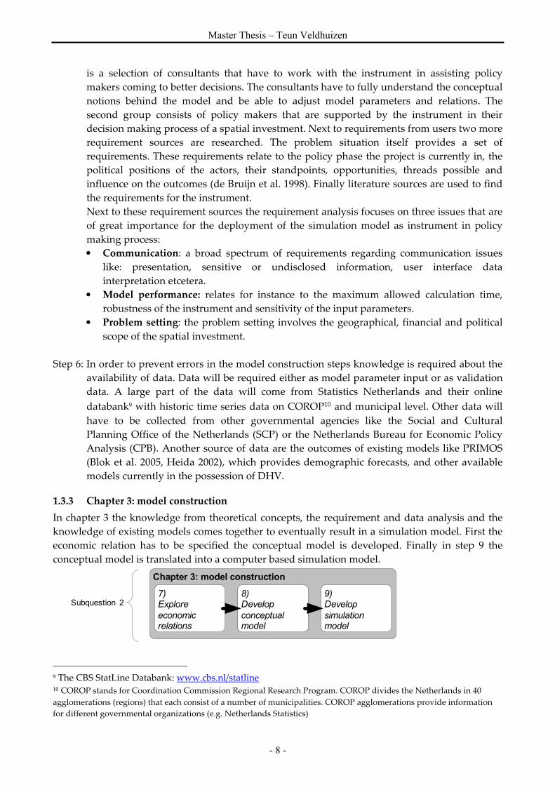
1.3.3 Chapter 3: model construction
In chapter 3 the knowledge from theoretical concepts, the requirement and data analysis and the
knowledge of existing models comes together to eventually result in a simulation model. First the
economic relation has to be specified the conceptual model is developed. Finally in step 9 the
conceptual model is translated into a computer based simulation model.
9 The CBS StatLine Databank: www.cbs.nl/statline 10 COROP stands for Coordination Commission Regional Research Program. COROP divides the Netherlands in 40
agglomerations (regions) that each consist of a number of municipalities. COROP agglomerations provide information
for different governmental organizations (e.g. Netherlands Statistics)
Chapter 3: model construction
8)Develop
conceptual model
9)Develop
simulation model
7)Explore
economic relations
Subquestion 2

Understanding economic effects of spatial investments
-9 -
Step 7: In step 7 a link is made between the prior knowledge of existing models, economic
literature and the requirement analysis by exploring the economic relations. From the
requirement analysis the desired output variables are known (what information is
demanded) and using the literature the underlying relationships are analyzed further. The
relationships will have to be quantified and causal loops have to be identified.
Step 8: The variables and relations from step 5, 6 and 7 form the basis for the conceptual model of
the instrument. In order to prevent a profusion of variables and causal relations that would
obscure transparency a selection in variables is made. The conceptual model entails all the
major economic relationships and in turn provides a basis for the final simulation model.
Step 9: With the base model up and running the case specific model(s) can be built. The case
specific model accounts effects that are dedicated for a specific region. The case model is
tailored to give answers to specific questions the client has, as not every client is interested
in the same output data.
1.3.4 Chapter 4: model validation and requirement testing
Now the conceptual model has been translated into a simulation model the simulation model
needs to be tested and validated. In the validation process two important issues are analyzed: the
ability of the instrument to reflect reality and the internal consistency. In chapter 4 the question of
the practical applicability plays a central roll (sub question 3). This includes the applicability of the
instrument in multiple regions and for multiple project types.
Step 10: The model that was built in step 9 is now ready to be tested. It has to undergo the
validation and verification process as is common for simulation models (Sterman 2000).
The most important steps include:
• Boundary adequacy: tests if the behaviour and outcomes (the best policy) of the model
changes under different boundary assumptions.
• Structure assessment: checks the structure of the model, does it reflect the behaviour of
real actors, is the aggregation of the model well chosen.
• Extreme conditions test: will the model still make sense when inputted with extreme
values.
• Surprise behaviour: does the system react appropriately to new conditions or does it
show unpredicted behaviour.
Special attention needs to be given to the sensitivity analysis of the input variables and the
input parameters. Small changes in the variables that cause big deflection in the output of
the model should be identified and studied. The time series model output will also be
tested against output of other models; this way a comparison can be made in the relative
accuracy of the model (Forrester 1980). Section 4.1 gives a more detailed description of the
validation process and the different validation procedures.
Chapter 4: validation and requirement testing
10) Execute model
validation
12)Test
requirements from step 4
Subquestion 311)Test
applicability

Master Thesis – Teun Veldhuizen
- 10 -
Step 11: Now the model has been validated, step 11 will test the applicability of the simulation
model. The instrument will be tested on the ability to represent reality and make valid
claims about the development of the socio-economic indicators. For this purpose the
simulation model will be run with historic data in order to check if the results actually did
come true.
Step 12: In step 12 the requirements from step 4 are tested with the validated instrument. It has to
be seen if all the requirements are implemented in the instrument and if the instrument
performs its tasks as desired. In order couple of tests are performed with different actors.
Model experts will analyze the mode structure while policy makers assess the usefulness of
the instrument in their line of work. In three separate group session the dynamics of the
instrument is tested on a larger group of people, like an actual consultancy assignment.
1.3.5 Chapter 5 and 6: thesis conclusion and reflection
In chapter 5 (step 13) the main research question is answered and the sub questions are elaborated.
Subsequently in chapter 6 (step 14) a reflection on the project is described, what can be learned
from the project and what might still be improved?
Step 13: In step 13 the research questions can be answered using the experience from performing
the requirement analysis, building the simulation model and validating the results.
Step 14: The final step of the thesis project is reflecting on the thesis project. The reflection consists
of two parts. The first part is a set of recommendations for further research into the use of
system dynamics in economic models. The second part reflects on the developments and
decision made during the course this thesis project. This will give an idea of the insights
gained in the process of developing the thesis model and writing this report. The second
part is a reflection on the general applicability issues of the developed model in practice
and dealing with available data.
1.4 Introduction of case study: Wieringerrandmeer
The case used in this thesis is the Wieringerrandmeer (WRM) project. It is located in the North of
North-Holland and concerns a small rural area with two municipalities: Wieringen and
Wieringermeer (see figure 1.2). The project involves the formation of a new lake in the polder and
the creation of 1845 new dwellings in the vicinity of the lake. The case will be illustrated with a
very brief history and the coming about of the plan to redevelop the Wieringermeer polder. The
following section will give an overview of the project that has been proposed, giving insight in the
Chapter 6: reflectionChapter 5: conclusions
13)
Answer
research questions
14)
Reflect on
thesis project

Understanding economic effects of spatial investments
-11 -
scale and scope of the project. The timeline of key policy decisions is set out in section 1.5.2 and in
1.5.3 an actor analysis is performed.
1.4.1 From lake to polder back to lake again
The Wieringermeer polder is located in the top of the province of North-Holland. The polder was
created between 1927 and 193011 as part of a large land reclamation project in the Netherlands. The
polder currently functions mainly as
land for agriculture; this function
however has been under discussion over
the past years. The Wieringermeer
polder is a rural area situated about 55
kilometres north from Amsterdam. A
problem in the region is the increasing
departure of younger people and the
general trend of an aging population.
One of the consequences of this
demographic development is a fading
support for services and facilities in the
region. Meaning that retail, recreation,
healthcare and cultural functions will
retract from the region (DHV 2006). The
region also has some other issues; there
is a need for improved water
management for the irrigation of
farmland and there is an ambition of
creating an ecological link between the
Waddenzee and the IJsselmeer (see also
figure 1.3).
Figure 1.2, province of North-Holland (Source: Google Earth)
Figure 1.3, the Wieringerrand-
meer project area (Source:
Google Earth)
11 http://nl.wikipedia.org/wiki/Wieringermeerpolder (visited: March 3, 2006)
Wieringerrand-meer project
area
0 4 8km
Wieringermeer polder
Amsterdam
Wieringen
0 12,5 25 km

Master Thesis – Teun Veldhuizen
- 12 -
In order to solve these problems the municipalities of Wieringen and Wieringermeer and the
province of North-Holland issued a contest. This contest resulted in a public private partnership
that was given the task of developing new economic impulses for the region as well as solving the
water management issues. These impulses were focussed on12:
• Red development: socio-economic development. The attraction of more and different labour
and inhabitants to the project region
• Blue development: improvement of water management. More high quality irrigation water
supply for agriculture activities and better water storage facilities.
• Green development: realisation of robust ecological link. Nature reserve as level crossing for
flora and fauna between the North Sea and the IJsselmeer.
The Lago Wirense consortium won the design contest. This three party consortium consisting of
Volker Wessels Stevin Bouw & Vastgoed Ontwikkeling Nederland BV, Boskalis BV and
Witteveen+Bos BV proposed a plan that would transform the Wieringerrandmeer into a pleasant
atmosphere for living and recreation (Lago Wirense 2004). The project area is indicated in figure
1.3 and illustrates the current situation. Figure 1.4 is taken from the Lago Wirense proposal and
shows the lake forming a connection between the Amstelmeer in the southwest with the IJsselmeer
in the northeast. The project will span some 25 years to complete with end date estimated in 2030.
The dwellings that Lago Wirense intends to build are only owner-occupied houses in the mid- a
higher segments. Most of the dwellings will have a lake or forest view. The intention of Lago
Wirense is to draw higher incomes into the project region in order to maintain the level of services
and facilities. The north side of the lake will consist of reed canes and shallow water forming the
ecological link between the North Sea and the IJsselmeer. Lago Wirense also intends to improve
the water sport qualities of the project region by creating yacht-basins and locks both tourist and
professional opening up of the lake area. The locks will also enable passage from the Amstelmeer
to the IJsselmeer for professional and recreation traffic.
Figure 1.4, the Wieringerrandmeer project area (Source: Lago Wirense, May 2005)
12 Stated in the consultation document from 9 April 2003. Accessible trough the Wieringerrandmeer website:
http://213.201.212.154/_clientFiles/{A01A823B-4CC5-4779-B99C-68E25ABFA950}/PPS_consultatie.doc (visited
on 01-06-2006)
0 4 8km

Understanding economic effects of spatial investments
-13 -
1.4.2 Policy time line in the Wieringerrandmeer project
The initial idea for the re-flooding of the Wieringermeer polder has been around since the late
nineteen eighties when it was proposed by a member of the Provincial States. Several researches
were executed and plans were drawn up under that cover of a programme called: “Water Bindt”.
Eventually in 2002 the developing agency “Wieringerrandmeer” was put up, consisting of the
municipalities of Wieringen and Wieringermeer, Polder board Holland’s Noorderkwartier and the
province of North-Holland.
The series of important events between January 2003 and June 2006 are depicted in a timeline in
figure 1.5. The kick-off for the current state of play was given in May 2003 with the announcement
of a contest. This announcement was sent out to a range of firms and organisations, the
“Consultatie document” made the intentions for the region clear. The document also presented
initial ideas for the possibility of public-private-partnership in the development of the region. The
actual competition started in November of 2003 and an independent jury announced the winner in
February 2004. As mentioned above, the winner was the three-headed consortium Lago Wirense.
In the following period the plans of Lago Wirense were worked out in dialogue with the province
and municipalities. The worked out plans resulted in an intention agreement, this agreement
clarified responsibilities, a worked out project plan and a detailed public structure.
Jan-03 Aug-06
May-03Competition anouncement
Nov-03Start of
competition
Feb-04Jury decision
on winning project
Oct-04Intentionagreement
Mar-05Signed intention
agreement
Nov-04Agreement denonced byWieringen
Mar-06Settlementof IER
Jun-05Initial IER andpublication of agreement
Figure 1.5¸ important events in the Wieringerrandmeer policy process
Then in November of 2004 the town council of Wieringen denounced the intention agreement. All
the other parties had signed in favour of the project, including the mayor and administrators of
Wieringen. After the rejection some a cooling off period was agreed between all parties. The town
council of Wieringen demanded more knowledge and better-funded estimations on the financial
risks for both municipalities. During the cooling off period the financial plans were clarified and
Wieringen eventually signed the intention agreement in March of 2005.
The next step in the policy process was to develop and Integral Effect Study (IER) which included
effects for agriculture, the economic position of the region and a social cost benefit analysis. The
early findings of the IER were presented in June of 2005 and after revision of all parties the final
version was presented in March 2006. According to the project planning construction should start
in 2007 and will take until 2030.
1.4.3 Actor analysis of the Wieringerrandmeer project
The most important actors in the development of the Wieringerrandmeer are:
• The province of North-Holland: the North-Holland has great interest in improving the North
of their province as it lacks in economic performance compared to the south of the province
(Amsterdam and Haarlem). They acknowledge the negative side effects of the aging
population in the region (see also 1.4.4). The Province of North-Holland also acts a financier of

Master Thesis – Teun Veldhuizen
- 14 -
a part of the project and is risk bearing involved in the successful implementation of the
project. The province has therefore great interest in that the project is executed, preferably with
funds from the central government.
• The municipality of Wieringen: Wieringen is a municipality situated on the old Wieringen isle
(see figure 1.4) and the inhabitants are the “original” residents of the region. Wieringen is a
small municipality with little over 8000 inhabitants (CBS 2005) who see the development of the
new lake as the end of their beloved quiet landscape. Another part of their reluctance is the
financial size of the project and risks their municipality runs. They fear that the project is too
big for the small, rural municipality of Wieringen; they simply do not have the manpower or
the expertise. More subjective is their stance towards the city of Wieringermeer, which they
deem not “original” and intrusive (interview Stegeman 23-12-2005). The community itself is
divided over this issue, which is represented in their municipal government.
o The city council of Wieringen: the city council of Wieringen initially opposed the idea of
the new developments but could be persuaded by their neighbouring city Wieringermeer
and the Province of North-Holland. The city council acts directly on behalf of the
inhabitants who are not pleased with the new developments and are concerned with the
financial risks.
o The administrators of Wieringen: the city administrators initially approved the new
development plans and agreed immediate cooperation. They indicate that swift action is to
be taken in order to prevent a deterioration of the economic situation of their municipality.
• The municipality of Wieringermeer: Wieringermeer is the municipality that was developed
after the creation of the new Wieringermeer polder in 1930. The municipality has some 13000
inhabitants and is, compared to Wieringen, a new town. The municipality of Wieringermeer is
great supporter of the WRM project as they see the necessity for change.
• Polder board Hollands Noorderkwartier: the polder board has to insure high quality and
sufficient quantity of water in the project region. They are not part of the development team
and are not financially involved. They do however act as advisory organ for the project and
assist in the information provision of the consortium.
• Lago Wirense: the winning project team of the contest for the development of the
Wieringerrandmeer. Lago Wirense consists of the three companies: Volker Wessels Stevin
Bouw & Vastgoed Ontwikkeling Nederland BV, Boskalis BV, Witteveen+Bos BV. The aim of
Lago Wirense is to profit from the project.
The problems that the project currently13 faces are reaching agreements on specific details of the
basic agreement made between March and May 2006. The municipalities want to steer clear of any
large risky financial commitments because that could damage their municipal funds. This means
that the municipality and the central government have to bear more risks. Lago Wirense is
working out more and more details of the project and is trying to avoid unforeseen costs like
problems with the soil stability, ground pollution etcetera. The province remains confident that all
obstacles van be overcome and that final agreement can be reached this summer (Meetings with
Arjan Stegeman from Lago Wirense (11-05-2006) Wim Voordenhout from the province of North-
Holland (23-05-2006). The province and Lago Wirense both will play a part in the requirement
analysis in chapter 2 and in testing the model in chapter 4. The simulation model will also be
tested in an environment with all actors present in a group (section 4.3.2)
13 Time of writing is 19-06-2006

Understanding economic effects of spatial investments
-15 -
1.4.4 Socio-economic analysis of the Wieringerrandmeer region
This section analyses the socio-economic status of the Wieringerrandmeer region. The WRM is
compared to the average data from the Netherlands. Data from the CBS is used to calculate the
current and historic performance of the region. For the future demographic developments data
from the PRIMOS model is used. The socio-economic analysis focuses on three issues:
1. Employment in the region
2. Demographic development
3. Economic development
1. The rural character of the region sketched in previous sections can also be found in the regional
industry sector structure. Employment in the production sector is heavily overrepresented
compared to commercial services (see table 1.1). The share of production sector labour
(agriculture, industry and construction industry) is almost twice as large as the national
average. The less developed sectors compared to the national average are the Health and
Wellness, Transport and Communication and Commercial Services. In total 5560 people work
in the WRM region.
Table 1.1, employment industry shares in the WRM region
2. The demographic situation in the WRM is currently not that different from the national
average. In the WRM region about 21 thousand people live in almost 9 thousand households14
(CBS 2005). Table 1.2 illustrates the age distribution in the column “Share in 2005 (%)“; this is
the percentage of people in an age group for the Netherlands and the WRM region. The WRM
region has relatively more people between 45 and 65 and relatively less people between 15 and
44. Currently that is not a problem, however the demographic projections until 2030 show a
potential problematic situation. The columns on the right side of table 1.2 show the index of
predicted development of the age groups. What can be noticed in the Netherlands is the
tremendous increase of inhabitants older than 65. This group will grow with 67 percent in the
next 25 years. In the same time the other age groups will grow only slightly or even get
smaller. The WRM region shows the about the same increase of older people. The big
difference between the Dutch average and the WRM region is that all the younger age groups
(0-65) will significantly decrease over the coming 25 years. This “de-greening” of the region can
potentially cause problems. For instance the region might lack in providing substantial
facilities and services like pharmacies, grocery stores or doctors.
14 For the Netherlands in 2005: 16,4 million inhabitants in 7,1 million households (CBS 2005)
Emplployment: share of industry sectors (2004)
volume percentage
Total jobs (x1000)
Agriculture
Industry
Construction
idustry
Trade
Transport and
communication
Financial
institutions
Com
mercial
services
Health and
wellness
Other, non
commercial
services
Netherlands total 6.929,4 1% 13% 5% 17% 6% 4% 20% 16% 18%
WRM region 5,6 8% 22% 8% 19% 3% 2% 13% 9% 16%

Master Thesis – Teun Veldhuizen
- 16 -
Table 1.2, age development in the Netherlands and the WRM region
3. The economic development of the WRM region is likely to stay behind the Dutch development.
Partly because there is an overrepresentation of production sector labour in the region, which
has less added value then for instance the commercial services sector15. Secondly because the
potential labour force in the region (inhabitants between 15 and 65 years old) will decrease
over the next 20 years (see table 1.2). This has two effects: first the gross added value of the
WRM region will decrease, reducing the economic activities in the region further. Secondly the
disposable income of the households in the region will decrease due to the fact that more
people live on their pension (which is lower than regular salary). This will lead to lower
spending in the region, which in turn means that even less products can be sold and produced
in the region.
From the economic analysis it can be concluded that the current socio-economic status of the
region is similar to the national average. However future developments predict that the region will
economically suffer from the aging inhabitants. The growth in the younger age groups (0-15 and
15-30 stays far behind compared to the national average. This could have consequences for the
level of services that is offered in the region as the basis for these services diminishes.
15 The CPB predicts a lower growth of the production sectors compared to the trade and commercial services
sector (Huizinga 2004).
Inhabitant age developments
index, 2005=100
Share in
2005 (%)
2010
2015
2020
2030
Netherlands 0-14 year 19 98 96 94 97 Netherlands 15 - 44 year 41 97 95 94 96 Netherlands 45 - 65 year 26 109 112 113 102 Netherlands 65 year plus 14 109 126 139 167
WRM region 0-14 year 19 96 92 88 90 WRM region 15 - 44 year 39 96 91 90 89 WRM region 45 - 65 year 28 103 104 103 91 WRM region 65 year plus 14 115 135 151 171

Understanding economic effects of spatial investments
-17 -
2 Model conditions and environment
In the second chapter the first sub question is worked out and supported by steps 4, 5 and 6. The
focus of this chapter is therefore on attributes of other economic models and demands potential
users of the instrument.
What are the leading indicators and underlying relations of an instrument for the ex-ante exploration and
assessment of policy options in spatial investments in a region?
a. What are the user requirements of such an instrument?
b. What can be learned and used from the existing models or instruments for regional economic
analysis?
c. What are the generally accepted data sources that can be used as input parameters for such an
instrument?
Before these sub questions can be answered a better definition must be given of the intended
properties of the policy-supporting instrument. Therefore section 2.1 gives a description of what is
meant with policy supporting models and the place of the instrument in the policy life cycle. The
latter indicates the policy phase in which the instrument should be deployed. Section 2.2 gives a
definition of the geographical scale of the instrument. The former definitions are needed before the
requirement analysis can be performed in section 2.3. The requirement analysis illustrates the
demands for the simulation model from different sources, both literary as user oriented. Using the
outcomes of the requirement analysis a set of existing models is researched that approximates the
functionality of the thesis instrument. From the existing models a great deal can be learned that
might prove useful in the construction of the thesis instrument. Section 2.4 ends with a
specification of why the currently existing model cannot fulfil the demand posed in the
requirement analysis. This specification leads to the introduction of system dynamics in section
2.5. The basic methodology, principles, pros and con’s of system dynamics are mentioned in this
section, ending with the proposal to system dynamics for the thesis instrument. From studying the
existing models and the user requirements a fair indication can be given on what information is
needed to construct and operate the thesis model. This subject is given attention in section 2.6 were
an indication is given of required data and the location of this data. Finally in section 2.7 the
question is answered what the leading indicators of the instrument should be.
2.1 Policy making and simulation models
Simulation models have had large impacts on the way policy makers perceive the world and
develop new policies. It was the World3 simulation model from Donella H. Meadows that was
used by the Club of Rome in the 1972 resulted in the well-known publication Limits to Growth
(Donella Meadows 1972). The simulation model helped to raise awareness with many policy
Chapter 2: model conditions and environment
5) Research
existing models
4) Perform
requirement analysis
6) Research data
availability
Subquestion 1

Master Thesis – Teun Veldhuizen
- 18 -
makers that economic growth was not infinite and that the natural resources would eventually run
out. Another, more recent application of models in policy making are the projections made by the
CPB based on the political programmes of the different Dutch political parties (CPB 2002). The
JADE model calculates the effects that result from the suggested policy programmes (CPB 2003).
2.1.1 Policy decision models and policy supporting models
A distinction must be made between decision models and policy supporting models. A decision
model specifically aids policy and decision makers in making a choice between two or three policy
options. Such a model must present the outcomes in a manner that it supports a binary decision.
This decision is either go ahead with the project or terminate it. Social cost benefit analysis (SCBA)
is an example of a model that assists in decision-making. It evaluates all possible effects and
attaches a financial compensation to each of the effects. Then in the final step of the analysis the
total costs are deducted from the total benefits, the answer is either a positive or negative balance
(Eijgenraam et al. 2000). SCBA will be addressed in more detail in section 2.3.4.
A policy-supporting model is aimed at aiding policy makers in gaining insight in the economic,
social, demographic or environmental effects. A policy-supporting model is most valuable in the
early phases of policy development. This in contrast with a decision-supporting model, which is
needed right before the moment the final decision on the project is made. The value and necessity
of quantified information early in the policy process is one of the recommendations of the
Committee Duivensteijn (TCI 2004). The committee also noted that risks were identified too late in
projects and when discovered were not discounted in the budget (TCI 2004, p 32). The thesis
model will have to supply the required quantified information on socio-economic effects on a
regional scale level and be able to give some idea to what risks are involved.
2.1.2 The place of the thesis model in the policy life cycle
Policy concerning multi million euro investments from both public and private parties does not
come about over night. It is a painstaking process of debilitation, politics and persuasion to come
from initial idea to the final
decision. A method for studying
policy processes more accurately
is presented by Winsemius
presented over two decades ago.
The policy life cycle (PLC) for
environmental issues, as
described by Winsemius (1986),
gives an idea of how issues
surface on the political agenda
and eventually turn in to actual
policy (see figure 2.1). Starting at
the beginning: at certain moment
in time a problem is recognized. The
recognition can for instance occur
through party politics,
international agreements and
media attention.
Figure 2.1, policy life cycle and modelling roles
Recognition
Policy implementation
Policy formulation
Control Problem
MediaRole 1Eye-opener
Role 4Management
Role 3Consensus
Role 2Argument
Winsemius’ policy life cycle
Different model roles

Understanding economic effects of spatial investments
-19 -
In the second phase of policy life the problem is formulated in debates and research, the conditions
for a possible change are set. In the next phase the policy is implemented, therefore the formulated
policy will have to be translated into actual mechanisms and regulations. Finally, the policy
execution will have to be brought under control, which will eventually either solve the initial
problem or not. Winsemius’ cycle was designed for environmental issues in policy development,
however in this research the use of the PLC model is extended to regional development issues as
well.
The relation between the PLC model of Winsemius and quantitative models has been researched
and described in the article of van Daalen, Dresen and Jansen (2002). In their article they attribute
four different roles to models within the policy life cycle:
1. Models as eye-openers: models are used to put certain issues on the political agenda, the
best example of such a model is mentioned above: the World3 model. World3 led to the
Limits to Growth report (Donella Meadows 1972).
2. Models as argument in dissent: in this role the model functions as an argument in a debate.
The outcome of the model can also be used as counter expertise to challenge the outcome of
another model, however this effect is unwanted. In some cases the term “report war”
(rapporten oorlog) was used by the TCI (2004). In this phase however an effect model can
render poor policy propositions obsolete in an early stage or promote other that have
prospering effects.
3. Models as vehicles in creating consensus: in this phase a model can assist in creating
political consensus. This could for instance happen by creating shared knowledge
(Richardson 2004) in a group model building session. Shared knowledge can be used in
discussions where two parties try to reach an agreement based on the same data.
4. Models for management: a management model gives insight in the effects of implemented
decisions and helps to identify concrete policy decisions. An application mentioned in the
text is finding the optimal level of source extraction (van Daalen 2002).
This PLC provides a basis for the positioning of the thesis model in the policy life cycle. The aim of
the model is to assist policy makers in an early phase and to develop a policy-supporting model.
This would implicate that the thesis model should support the policy formulation and policy
implementation phase. Thus, model role 2 and 3 become the focus roles for the thesis model. Role
4, management does implicate the policy implementation phase, however this role is more
associated with decision models and therefore not included in further research.
When the Wieringerrandmeer project is analysed in terms of the policy life cycle, it has to be
concluded that project is currently between phase 2 and 316. Almost all the development plans are
worked out in the policy formulation phase and a management organisation has been set op for
the control of the project. The final decision for the project awaits a final analysis on the social
benefits of the project that Witteveen+Bos and DHV are currently working on.
16 Time of writing is 19-06-2006

Master Thesis – Teun Veldhuizen
- 20 -
2.2 What are regional investment projects?
The model that will be developed has to evaluate regional investment projects. The question is
how big is this region or project? This section will clarify the term regional investment project and
try to illustrate the type of effects that occur on this level and that are important for the policy
makers.
2.2.1 Geographical scale and the project region
For this thesis project the Wieringerrandmeer case study is used as an example of a regional
investment project. The scale of this project however does not fit exactly in the commonly used
geographical levels. The scale levels that are universally used are:
• Neighbourhood level (radius approximately 0,1 kilometre): this is the level of small groups of
streets that have similar characteristics
• District level (radius approximately 0,5 kilometre): the level consists of a group of
neighbourhoods that typically have a (small) centre.
• Municipality level (radius approximately 3 kilometre): the municipal level is a collection of
districts; this can also mean a set of dispersed smaller municipalities. The municipality of
Wieringen consists for instance of 8000 inhabitants.
• COROP level (radius approximately 20 kilometre): the Netherlands is divided in 40 COROP
regions each consisting of roughly 350.000 inhabitants and 150.000 jobs. A COROP level is
constructed from the summation of the set of municipalities within the COROP region.
• Provincial level (radius approximately 50 kilometre): a province is a part of the country and
consists of a set of COROP regions
• National level (radius approximately 150 kilometre): a nation
The thesis model focuses on a level between that of the municipality and the COROP level.
Statistics Netherlands has more data available as the geographical scale level increases, meaning
that for data usage a COROP level will have more data available then the municipal level. Because
the thesis model is focused on a multi municipal level, data from the COROP level will be used
when municipal data is lacking.
2.3 Finding the model requirements
The development of the simulation model is started with a requirement analysis. The general idea
that functions as point of departure for this requirement analysis is based on the concept of a
simulation model. This model supports policy makers in the development and testing of policy
alternatives in spatial issues (non-infrastructure). The model is able to test the effects of different
policy options/alternatives under different economic scenarios. The model can be seen as an
instrument for providing quantified data, early in the policy life cycle. The instrument as
developed in this thesis is only applicable for spatial planning projects on a COROP and multi-
municipal (> 20.000 inhabitants) scale. Furthermore it supports interaction between consultants
and policy makers through an interactive user interface. From this viewpoint the requirement
analysis takes off.

Understanding economic effects of spatial investments
-21 -
For the thesis model interviewing has been chosen as requirement trawling technique. Interviews
can be executed from remote locations via telephone; furthermore they do not (as work shops do)
require complex meeting arrangements or long introductions. The interviews follow an open line
of questioning to promote the respondent to think of unconscious and undreamed requirements.
Interviewing is also the best way to reach respondents that are situated at different locations, as
group brainstorms require all people to be in the same room. Some interviews with policy makers
and consultants who were familiar with model building resulted in discussions and brainstorms
about the requirements the model should have. More information on the decision to use
interviewing can be found in appendix 2. In this appendix information about requirement trawling
are also included, it also explains where, during the interviews special attention was paid to.
2.3.1 Creating structure: a requirement analysis framework
Now a requirement trawling technique has been chosen and it has been made clear that both
consultants and the policy makers should contribute to the requirement trawling process a
framework is presented. The framework has three requirement sources and three dimensions that will
provide structure and help to streamline the process. The requirement sources are the sources of
information that contribute to the final list of requirements. The three dimensions stress the
important issues concerning the development of the simulation model. Figure 2.2 shows the
framework of requirement sources and dimensions. Using this framework two questionnaires
were made to function as a guideline during the interviews (see appendix 3 for the questionnaires).
The requirement sources are:
• Policy makers: the role of the policy makers during the interviews is to convey how they see
possibilities for a simulation model to aid them in improving policy development. Further
more policy makers have a better understanding of where to use a simulation model in the
policy life cycle. Should it be used as persuasive argument in a dispute or as facilitation of
bringing about a change in the public opinion?
• Consultants: consultants have to see the simulation model as an instrument that is to be used in
providing advisory services. They have to indicate if and how they want to change input
parameters, add variables and calculate different scenarios. Consultants will be asked for their
requirements concerning the development of a simulation model and the use of the model with
policy makers.
• Policy issue: requirements that stem from the policy issue are specific for each case the
simulation model is used for. As each case is different each case requires different steering
variables and different socio-economic effects. For instance, for the Wieringerrandmeer case
the simulation model must indicate the growth of the housing stock and the effects that has on
the demographic composition of the municipalities.

Master Thesis – Teun Veldhuizen
- 22 -
Figure 2.2, requirement analysis framework
Next to the three sources of requirements (vertical axis), three dimensions are identified (on the
horizontal axis in figure 2.2). These dimensions cover the most important aspects of the simulation
model and will form the basis for the line of questioning during the interviews. For each different
requirement source these aspects entail different issues. The list below clarifies the dimensions
further:
• Communication: the aspect communication is important for the transfer of information both
from policy maker to consultant as visa versa. For instance for the consultant this means that
he or she has to consider the background of policy makers, and policy makers must be open to
a new policy-supporting instrument. The structure of the model must on the other hand
support the complexity of the problem and the level of detail of the policy maker’s issues. An
important goal of the thesis model is to convey information to the policy maker concerning
assumptions and premises that precede the model construction in chapter 3. These
assumptions can vary from economic scenarios to assumptions on the power of attraction of
the region. Requirements that follow from the policy issue are given in terms of factors that are
important for that specific issue. In case of an investment in regional employment, detailed
factors concerning employment will need to be incorporated in the simulation model.
• Model performance: from the model performance follow requirements that indicate limits of
model concerning sensitivity, calculation time and risk analysis. The quality of the input data
that is used also plays a role in the performance of the model and has implications for the use
of the outcomes. For the policy maker it is important to have some insight in the bounds and
the accuracy of the model.
Communication
Model
performance
Problem setting
Information retreaval from client
User interface for consultant
User interface for model policy maker
Calculation time
Product promotion , selling point
Indication of outcome bounds
Model structure
Operationalisation of problem variables
Validation
Scale: timeline, geographic , financial
project sizeReusability of the model
Critical factors
Accuracy
Scenarios
REQUIREMENT SOURCES
Policy makerPolicy issueConsultant
Preparation time Risk analysis
Function in policy process Function in policy
process
Communication of assumptions

Understanding economic effects of spatial investments
-23 -
• Problem setting: the problem setting also is a source of requirements. For consultants the fact
that the simulation model must be a profitable product is important. The use of simulation
models in policy formulation must have unique selling point for them. As for the policy
makers, they need to recon with their political arena and alliances. They have to be aware of
the model use: do they require the model for project appraisal or for scenario development or
do they seek justification for a specific investment they are interested in? The policy issue and
the problem setting give an overview of requirements that can stem from the specific policy
issue in a larger political setting.
2.3.2 Setting up the interviews
With the requirement analysis framework as a basis, two questionnaires are formulated, one for
the policy makers and one for the consultants (see appendix 3). The content of both questionnaires
is generally the same and both use the three dimensions from the framework as guideline. They
differ on specific issues like the perception of information, usability of the instrument and
performance requirements. The interviews are conducted in an open line of questioning in order to
promote creative thinking during the interviews. The average time for an interview is 1 to 1,5 hour.
Each interview is divided into 3 parts:
1. The interview starts with some general questions to test the respondents’ knowledge of
simulation models and mathematical modelling in general. Some respondents have used
financial models or have worked with the outcomes of mathematical models. Due to the
open structure of the interviews an experienced model user can give input and
requirements on a higher level. Other respondents that are for instance more focussed on
the implications of a simulation in a multi actor setting focus more on that particular
subject.
2. The general questions are followed by a short explanation of the simulation model that will
be developed. This will give the respondent some idea of what the intended model is
capable of and what it can be used for.
3. The next part of the interview is a series of detailed questions on requirements of the
simulation model. The questions are grouped so that they fit the three dilemmas from the
requirement analysis framework. Starting with communication followed by questions on
the model performance and the problem setting.
In total ten respondents with different backgrounds have been interviewed (see appendix 4 for list
of respondents). This group of ten respondents is divided three groups. The first groups are three
policy makers related to the WRM case study. The second group is a selection of five consultants
with an expertise varying from risk management, cost benefit analysis to economic modelling and
environmental effect analysis. Finally two model experts were interviewed to put the requirement
analysis in perspective and shed light on possible pitfalls in the construction of the model.
After the interviews the answers, quotes and remarks are grouped together in a long-list (see
appendix 5). This list gives an indication of the broad bandwidth of ideas and modelling concepts
put forth during the interviews. The long-list is screened for actual requirements; quotes and
general remarks are taken out and included as clues for the development of the model. These
remarks give information on the background of requirements or illustrate personal issues of the
respondents. This extra information led in most cases to the discovery of more requirements if

Master Thesis – Teun Veldhuizen
- 24 -
more detailed questions were asked. After the screening a long-list with requirements remained
that could be used for further processing.
2.3.3 Results: the requirements for the simulation model
The long-list of requirements resulting from the interviews described in the previous section
includes over 150 entries. Because not all of these entries are feasible requirements, a selection
needs to be made. This selection will be based on need-to-have and nice-to-have requirements.
Based on the intended functionality of the model (see section 1.2), the long-list is scanned and the
demands are grouped in need-to-have and nice-to-have requirements. The need-to-have
requirements will form the basis for the concept model in section 3.1. The nice-to-have
requirements should be kept in mind, it might be possible to include some of these requirements
relatively easy. An example of a nice-to-have requirement is that the model should be able to
calculate the financial return on investment for a private investor. This financial requirement does
not concern socio-economic effects and therefore it will not incorporated in the concept model (it
remains a nice-to-have requirement). A second selection that is made originates from contradicting
requirements that can be found in the long-list, these contradictions are design dilemmas. Special
attention will have to be paid to dilemmas that exist between the requirements of the policy
makers and those from the consultants. A striking example is the statement of policy makers that
most of the data should be presented in graphs while the consultants prefer presentation of
information in tables. How to deal with contradicting requirements is discussed in section 2.3.4.
The final list of need- and nice-to-have requirements is fully stated in appendix 7. The key need-to-
have requirements are selected and included in the main text below. The selected requirements
below are important because they illustrate a conceptual choice or because they are very
challenging requirements. The requirement are grouped in the requirement sources from the
framework:
• Policy maker requirements
• Consultant requirements
• Problem setting requirements
A second differentiation is made in the requirement analysis. For each of the three requirement
sources, three dimensions are specified. These dimensions are also used during the interviews. The
dimensions of communication, model performance and policy issue can also be found in the
requirement framework in figure 2.2. Finally an additional requirement source is added. Literature
requirements are included as an extra requirements source that originally fell out of the scope of
the requirement framework. However literature requirements appeared to be very useful in
delineating the model concept and in structuring the design process.
During the interviews with policy makers several issues kept coming
up. Issues that could not directly be translated into requirements by but
could prove important in the implementation of the model in a political
situation. Each interviewed policy maker made a remark concerning the level of detail of
information that is given to the policy maker in different actor settings. Some remarks that were
made:
• “The model must be able to deal with multiple levels of complexity in communication”
Policy maker
requirements

Understanding economic effects of spatial investments
-25 -
• “It must be able to change presentation styles, from comprehensive to simple”
• “The outcomes of the model must connect to peoples common sense in order to reach residents in smaller
municipalities”
These remarks point at the same issue: adapt the presentation of outcomes of the model to the level
of policy maker. In order to resolve this issue different interfaces must be built to make it suitable
for different actor groups. What becomes clear is that for the interactive use of the model, the
background and interests of the policy makers should determine as also the level of detail that is
presented to them. The time that is given for the interactive session must constrain the level of
detail. If for example only two hours are available, small details are irrelevant. Multiple interfaces
or levels of detail would make the simulation model broader applicable. Table 4.1 lists the other
policy maker requirements. The simulation model must:
Table 4.1, list of policy maker requirements
The interviews with consultants appeared more structured compared
to the interviews with policy makers. In more than one situation the
consultants contributed undreamed17 requirements while this occurred
less with the policy makers. The consultants also pointed out that it would be very important to
include an understandable manual with the model in order for them to work with it. It should
17 When a requirement is undreamed the respondent sees it as impossible while in fact it is a very important
requirement (see appendix 2).
Consultant
requirements
Policy maker: communication
1 Avoid using tables and use at the most 2 variables per graph
2 Be able to change presentation “styles”: comprehensive to simple
3 o Include a "Jip en Janneke” version explainable to laymen
Include the following factors
4 o Housing market and inhabitant development
5 o Employment
6 o Show 4 year policy cycles and economic growth
7 Not require more than 5 minutes on theory of system dynamics
8 The interactive session with client must not take longer than 2 hours
Policy maker: model performance
9 Include new variables (region specific) and remove absolete variables
10 Only use averages in the presentation of outcomes
11 Communicate reliability and the status of the model outcomes
12 Present uncertainties and assumptions in complete but orderly fashion.
13 Offer the possibility to calculate different policy scenarios
Policy maker: policy issue
15 Support gut feeling of policy makers
Communicate different stakeholders:
16o The residents of a region (they will influence local government)
17 o Other governments (for the creation of support)
18 o Other political parties for the (creation of support)
19 Be used in early phase of policy life cycle
20 Give indication of effects on provincial scale
21 Give indication of effects between small municipalities
22 Show result on a time scale between < 30 years

Master Thesis – Teun Veldhuizen
- 26 -
furthermore not be a requirement to be a mathematician or system dynamics expert in order to
work with the model. The interviewed consultants and the policy makers agree on the subject that
the simulation model can contribute more to the policy process if it is used in the start-up phase. A
consultant mentioned: “Research should foremost be executed to create clarity in fuzzy situations” and
“generation of alternatives that can immediately be quantified is a powerful tool”. The rest of the
consultant requirements can be found in table 4.2. The simulation model must:
Table 4.2, list of consultant requirements
The requirements that are obtained from the policy issue concern the
case for which the instrument is used. In this case the case the WRM
project. For the analysis of the socio-economic effects in the
Wieringerrandmeer the emphasis lies on the changes in the housing market and recreation
facilities that will affect production structure and the labour market. During the interviews the
respondents involved with the WRM project were asked specifically on detail of the WRM project.
The other respondents answered the questions on simulation models for supporting policy
development on spatial investments in general. The most important policy issue for the WRM
project is the exploration of the effects that extra tourism has on the region. Table 3.1 lists the rest
of the requirements. The simulation model must:
Policy issue
requirements
Consultant: communication
1 Be suited for the use with different actors and different regions
2 Present results in graphs with a maximum of 3 variables
3 Show relationship between input and output variables
4 o Highlight the policy steering variables
5 Show visual representation of model relations
6 The interactive meeting should take a half to a full day
Policy maker: model performance
7 Display additional variable information on demand:
8 o Standard deviation of outcomes.
9 o Input variable sensitivity.
10 o Reliability interval and model bounds.
11 Show distribution of uncertainty on output values.
12 Use sensitivity analysis for uncertain input variables.
13Make use of known modelling techniques like the PRIMOS model and the shift-
share method for estimating employment development.
14Clarify the relation between the thesis model and available models and
methodologies: Social Cost Benefit Analysis, REGINA etc.
15 The model outcomes must be reproducible results.
16 Store time-series outcomes in spreadsheet (Excel)
Consultant: policy issue
17 Present model outcomes in simplified “Jip & Janneke” versions.
18Give insight in the “mitsen en maren” of a project � show the model
assumptions.
19 Scale of the project the model should be suited for:
20 o Financial: > 10 million euro.
21 o Time span: 10 - 30 years.
22 One input screen for all the regional variables.
23 Use the model to gain insight on a provincial scale.

Understanding economic effects of spatial investments
-27 -
Table 4.3, list of policy issue requirements.
A requirement source that is not explicitly included in the requirement
analysis framework is the literature used in the initial phase of this
thesis project. Studying existing models that support spatial decisions
resulted in a range of issues that have to be dealt with in the simulation model. The important
requirements from the literature study are listed below in table 4.4. The simulation model must:
Table 4.4, requirements of the literature study
Literature based
requirements
Policy issue: communication
1 Very simple model interface
2 Understandable for laymen
3 Model must be able to deal with local communities and goverment
4 Give insight in the effect of tourism
5 o Day tourists and long holiday
Policy maker: model performance
6 Indicate the risk and uncertainty involved in the project
7 o Make a difference between Wieringen and Wieringermeer
8 o Uncertainty with respect to economic scenario
Policy issue: prolem setting
9 Illustrate the effect of stopping the project half way
10The model should facilitate a setting that will lead to a closer relation
between Wieringen and Wieringermeer
11 The model must show growth in retail, social services and recreation
Literature requirements
1Make a choice in the theoretical predicament of job-follow-people or people-follow-jobs
(Vermeulen & Verkade 2005).
2Differentiate a set of production sectors to indicate economic and employment growth in
these sectors (Heida 2002)
Include the following factors (Armstrong & Taylor 1993) and (Koops (2005):
3 o Labour market: working labour force, unemployment, jobs in region, vacancies.
4 o Demography: household size and composition, age, migration, birth/death rate.
5 o Gross added value.
6 o Attractiveness of region (through labour, residential or income advantages).
7 o Income: Regional wage level, consumption, average income.
8 o Real estate and land: supply of dwellings, demand of dwellings, price levels.
10
Include limited capacity of growth factors to prevent interpretation errors with
extrapolation (Nijkamp & Reggiani 1998). Major, one time events in the past may have
had a large effect on the historic growth. Extrapolating this growth without indication of
such an event happening again would be unjust and therefore growth (and decline) bounds
should prevent excessive growth.
11 The model must be able to indicate potential risks early in the policy phase (TCI 2004).
12 Show underlying assumptions of the modelling technique (Meadows 1976).
13
The model must not predict the future but give direction to the effects that a decision has
in the far future under different economic scenarios (Handbook of Knowledge Society
Foresight 2003). The model should be interpreted more as giving direction opposed to
providing a prediction (Koops & Muskens 2005).
14Always include expert opinions of non model-makers for specific regions (Forrester
1980).
15Develop the model in such a manner that it is possible to include other interesting
(unconventional) economic relations (Glaeser et al. 2001) and (Florida 2002)

Master Thesis – Teun Veldhuizen
- 28 -
2.3.4 Sorting out dilemmas and contradicting requirements
Because of the variety of respondents and the enormous size of the long-list with requirements
requirement some contradictions between requirements occur. These contradictions are treated
like dilemmas and will have to be solved before the conceptual design is made. Dilemmas do not
only indicate a contradiction between two requirements, they can also show the tip of a larger
“iceberg”. Some simple dilemmas can have huge design implications and can point out
weaknesses in the simulation model or concept. To make sure that these problems are not
encountered during the design of the model, dilemmas will be resolved in the following fashion:
1. First look for the underlying meaning of the dilemma. If indeed an iceberg is present at the
basis of this dilemma more attention should be given to the design choice.
2. The next step is to look for a simple solution that can make the issue go away. For instance
including both requirements if that is possible within the model and within the given time
constraints.
3. If the dilemma has not been resolved after the second step. The requirement with the
predicate need-to-have will get priority over the nice-to-have requirement.
4. When the conflict still has not been resolved the requirement will be chosen that is least
time consuming because the development of the simulation model is constrained by time.
Requirement dilemmas
• The duration of an interactive setting, 4 hours or 2 hours: this dilemma relates to the application of
the model with the end user. Depending on the setting, the time limit should be different. In
case of a presentation of the model outcomes, the time required should not be more than 2
hours. On the other hand, in an explorative setting, where policy makers are looking for
alternative solutions the required duration of the meeting can easily be 4 hours, even a day. A
solution to this dilemma would be to facilitate the model for short presentations and also for
more complex policy questions. This would mean that the model should be equipped with
multiple user interfaces with different levels of complexity. This requirement is already
recorded in the analysis.
• Displaying information on the meaning of the combination of two factors: a requirement from the
policy makers is to display the meaning of two factors in relation to each other. For example:
take two regions, both with low labour participation. A region with low income and low
labour participation indicates impoverishment and is therefore not considered a prospering
region. On the other hand a region with low labour participation and high income indicates the
presence of early retirees and can be considered a prospering region. The requirement to make
these relations clear should not be implemented. Model users should always analyze these
types of relations, as computers cannot judge them. A nice-to-have feature however would be a
“red flag” systems, that warns for unwanted combinations.
• Do or do not give information on variable bounds: policy makers tend to deem the indication of
variable bounds less important than consultants. The bounds of the outcomes can contribute to
better policy decision and should therefore be included in the model. The bounds should only
be displayed on demand, as the information is not relevant for all the model users.
• Keep the model presentation as simple as possible or present all uncertainties and assumptions: this
dilemma relates, just as the previous dilemma, to the level of detail of information that is given.
It should be possible to change this level and therefore both a simple presentation as a more
complex one should be provided.

Understanding economic effects of spatial investments
-29 -
Use the model on a provincial or small municipality level: the desire to apply the simulation model on
varying geographical scales is understandable. The requirements put forth by the respondents to
apply the model on a provincial or small municipality scale is not possible though. On a provincial
scale the model should incorporate more complex variables like province competitiveness, the
model is too simple for this scale. On a small municipal level the necessary information is not
available. Furthermore, on a small scale, small changes (for instance the departure of a local
grocer) present large deflections in the model that are not justified. The geographical scale of the
model will remain on a multi-municipal and COROP scale.
2.3.5 Reflection on requirement framework
The use of a framework for the requirement analysis proved useful for structuring the
questionnaires and the interviews (see figure 2.2). The framework gives some grip in thinking of
possible requirements. However, not all the requirements found during the interviews fitted into
this framework. Furthermore the literature requirement sources are not mentioned in the
framework and neither are the useful additions model experts. The literature requirements should
be explicitly included in this framework; this will also promote the use of existing list with
requirements. Interviewing model experts should also be included in the framework. Experienced
model builders in the field of regional economic modelling or system dynamics add value to the
relevance of the model. They can also warn the model builder for possible pitfalls and known
drawbacks of certain design assumptions and requirements.
During the development of the thesis model the use of a case study was chosen to make the model
more concrete. The issues for this specific case are dealt with in the “policy issue” in the
framework. These requirements are specific to that case only and should not be regarded as
general requirements. The specific case issue makes the requirements more focussed on the effects
of house-construction and recreation development. For new cases a short requirement analysis
should be performed on the policy issues. Using these case specific requirements the simulation
model can be tailored to fit the specific policy makers demands.
2.4 Existing spatial, regional economic models
This section will give a brief impression of existing regional economic that are relevant for this
thesis. An effort has been made by van Oort, Thissen and van Wissen (2005) in “A survey of spatial
economic planning models in the Netherlands” to create an overview of all the available models.
This wide range also includes models specifically for the assessment of infrastructure issues on a
national level like the RAEM model. Other models like PRIMOS produce forecasts on a municipal
level on the future development of population and household composition. The REMI model is
developed by the University of Massachusetts and domiciled by Ecorys. It claims applications in
infrastructure, main port, labour market, energy and environmental issues (van Bork & Treyz
2005). Four models are described in more detail in the following sections. The aim of this exercise
is to learn from these models and see if concepts and ideas from these models can be used in the
thesis model.
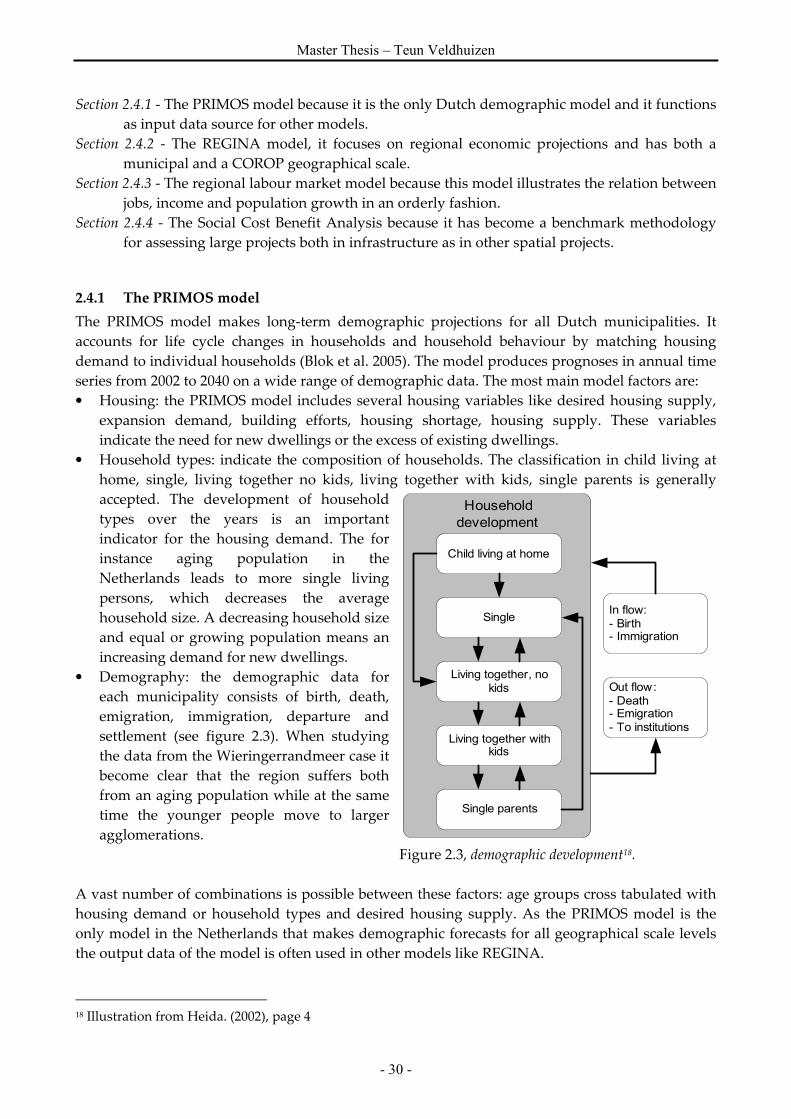
Master Thesis – Teun Veldhuizen
- 30 -
Section 2.4.1 - The PRIMOS model because it is the only Dutch demographic model and it functions
as input data source for other models.
Section 2.4.2 - The REGINA model, it focuses on regional economic projections and has both a
municipal and a COROP geographical scale.
Section 2.4.3 - The regional labour market model because this model illustrates the relation between
jobs, income and population growth in an orderly fashion.
Section 2.4.4 - The Social Cost Benefit Analysis because it has become a benchmark methodology
for assessing large projects both in infrastructure as in other spatial projects.
2.4.1 The PRIMOS model
The PRIMOS model makes long-term demographic projections for all Dutch municipalities. It
accounts for life cycle changes in households and household behaviour by matching housing
demand to individual households (Blok et al. 2005). The model produces prognoses in annual time
series from 2002 to 2040 on a wide range of demographic data. The most main model factors are:
• Housing: the PRIMOS model includes several housing variables like desired housing supply,
expansion demand, building efforts, housing shortage, housing supply. These variables
indicate the need for new dwellings or the excess of existing dwellings.
• Household types: indicate the composition of households. The classification in child living at
home, single, living together no kids, living together with kids, single parents is generally
accepted. The development of household
types over the years is an important
indicator for the housing demand. The for
instance aging population in the
Netherlands leads to more single living
persons, which decreases the average
household size. A decreasing household size
and equal or growing population means an
increasing demand for new dwellings.
• Demography: the demographic data for
each municipality consists of birth, death,
emigration, immigration, departure and
settlement (see figure 2.3). When studying
the data from the Wieringerrandmeer case it
become clear that the region suffers both
from an aging population while at the same
time the younger people move to larger
agglomerations.
Figure 2.3, demographic development18.
A vast number of combinations is possible between these factors: age groups cross tabulated with
housing demand or household types and desired housing supply. As the PRIMOS model is the
only model in the Netherlands that makes demographic forecasts for all geographical scale levels
the output data of the model is often used in other models like REGINA.
18 Illustration from Heida. (2002), page 4
Child living at home
Single
Living together with kids
Household development
Living together, no kids
Single parents
Out flow:- Death- Emigration- To institutions
In flow:- Birth- Immigration

Understanding economic effects of spatial investments
-31 -
The demographic projections are calculated through four key processes in the PRIMOS model:
demographic and household developments, regional migration, housing market dynamics and
housing production. All the processes take place on a geographic scale of municipalities. This
would also make it relevant for the use as input data for a model that has a multi municipal scale
like the thesis model. PRIMOS analyses inter and intra regional migration of persons. The model
deals with four migration motives that
together result in the total net migration
per region (Heida 2002, Blok et al. 2005)
(see figure 2.4). From these four motives,
employment migration is the most
important and significant factor for
migration. The PRIMOS model deals
with these migration motives by
including a factor that determines if a
change of job will lead to a migration
move based on the distance from the
current residence location and the new
job location. As this distance increases
the probability of migration increases
also. Residential migration takes place if
there is a mismatch between the current
and desired housing situation, for
instance in case of addition to the family.
Figure 2.4, migration motives.19
Residential migration occurs when the demand for a type of dwelling in a region exceed the
supply. Inhabitants will in that case start looking for dwellings of their desired type in other
regions. Educational migration is based on data from the “Referentie raming” from the Dutch
ministry of education, Culture and Science (OC&W). The Referentie raming predicts first year
student inflows in different educational bodies based on previous enrolment and city of origin of
the first years. Finally there are also some other migration motives. Some examples are
institutional homes and health care, cultural and leisure activities and landscape bound motives.
The PRIMOS model illustrates how models can deal with migration and demographic
development on a municipal level. However it fails to identify important economic functions like
the development of the gross regional product or the increase in jobs in the healthcare sector. A
model that does provide more economic data and still functions on a municipal level is the
REGINA model.
2.4.2 The REGINA model
The REGINA20 model is used to explain differences in employment and economic sector growth
between regions by analyzing the national growth, regional industry mix and other regional
factors. The REGINA model is developed by the Netherlands Organisation for Applied Scientific
19 Illustration from Heida (2002) page 5 20 REGINA is an acronym for Regionaal-Economische Groei IndicAtie
Employment migration
Cause: regional demand supply ratio employment
Migration motives
Migration patternsLeaving and settlement between regions
Other migration
Cause: facilities like medical institutions
Educational migration
Cause: by participating in and availability of
educational facilities
Residential migration
Cause: scarcity at regional housing markets nearby

Master Thesis – Teun Veldhuizen
- 32 -
Research (TNO), it uses the time series data from the PRIMOS model as forecast for the
demographic developments in all the municipalities of the Netherlands (Koops 2005). The
REGINA model is focused on forecasts of regional employment and the growth or decline of
production sectors in the Netherlands. Compared to the RAEM and PRIMOS model, the REGINA
model is relatively easy to comprehend. The mathematical basis that stands at its roots is called
shift-share analysis. Shift-share analysis extrapolates growth in production sectors through a shift
and a share part. The share part consists of the national growth indicators predicted by the CPB
(Huizinga & Smid 2004). The shift part consists of multiple variables with historical performance
as most important indicator (see also section 3.3). If, at regional level a sector performs admirably
compared to the national performance, an over-representation of that sector in a region will lead to
higher growth rates in the future (Armstrong 1993, Koops 2005). This compact theory is extended
by TNO to include other explanatory factors for industry and employment growth. As explanatory
variables for the over or under performance of a region the model uses the following factors next
to the industry mix:
• Labour supply: population growth increases the potential labour supply (age: 15-65), it also
increases the potential sales market.
• Agglomeration effects: from the New Economic Geography literature. REGINA includes an
explanatory variable for the proximity of concentrations of employment.
• Accessibility: as important attractor for firms to settle in the region.
• Proximity of economic main ports: the model takes Amsterdam Airport Schiphol and the
Port of Rotterdam into consideration.
• Sector representation: takes growth in economic sectors with different size into
consideration (using the Hirshman-Herfindahl index).
• Other factors: available space for economic activities, suburbanization.
The primary function however remains identifying differences in economic growth between
regions or municipalities, not the ex-ante calculation of regional investments. The use of the
PRIMOS model for the provision of demographic forecasts proves useful in the REGINA model. If
the model would also include a demographic module the relation would become exponentially
more complicated. And it would not be a guarantee the model would produce better results. The
REGINA model fails however to give policy makers insight in the inner workings of their model.
This would prevent the policy makers from understanding the effects of their decisions and the
consequences of their policy proposals.
2.4.3 The regional labour market model
The regional labour market model is built by the CPB focuses on the regional distribution of
population and employment (Verkade & Vermeulen 2005, Vermeulen & van Ommeren 2005 &
2006). The aim of the model is to provide long-term scenarios for policy development on
infrastructure projects and business development areas. The author uses the model to challenge
the popular believe that people follow jobs with the statement that the opposite is true; jobs follow
people. For both directions the causality theoretical explanations exist. Through a local
comparative advantage in production it is possible that wages increase, attracting migrants as they
start to rise, hence people follow jobs. The other way around indicates that as people move to areas
with high amenities (e.g. high quality services, attractive environment and consumer goods) they
supply labour, which attracts firms, hence jobs follow people (Vermeulen & van Ommeren 2005).
The regional labour market model acknowledges the fact that neither employment nor population
growth develops exogenous. Therefore the relations between them should be dynamic. The

Understanding economic effects of spatial investments
-33 -
geographical scale on which data is used in the model is on COROP level. For the model equations
are estimated on time series data from the 1970 – 2000 period. This makes the model more
econometric than other more theoretical derived model.
The two most important equations in the model are that of the net domestic migration (NDM) and
the employment growth (∆emp). NDM indicates the effects that the housing market, employment
and region specific amenities have on the migration in a region (see equation 1). The increase or
decrease in the housing stock seems to be the most important indicator for the NDM. The increase
of the housing stock with a 100 dwellings will lead to the increase of approximately 80 inhabitants
through migration based on the housing supply only. The negative 4% 1,1, −− − titi houpop indicates
the deviation from the equilibrium that occurs when the housing stock deviates from the national
average. Finally there is a positive impulse from employment growth in the region (∆emp). Note:
this factor is more than 26 times smaller than the effect from housing stock increase.
(1) k
tiktitititi
M
i
ti
tiXemphoupophouC
POP
NDM,,1,1,,
1,
,03.0)(04.08.0 α+∆+−−∆+= −−
−
NDM: net domestic migration
POP: population in age group 15-65
HOU: number of housing units
EMP: employment (employees in labour years)
C: region-specific fixed effect
X: other explanatory variables
The other basic equation of the labour market model is that of the growth in employment (see
equation 2). The employment growth in the region is largely based on the population (age group
15-65), which is an outcome of the hypothesis that jobs follow people. A smaller and negative
effect is attributed to the employment density ( 1,1, −− − titi popemp ). Under other explanatory
variables the regional labour model accounts for more significant effects. For instance the growth
that would be predicted based on the industry composition in a region, much like the sector shift
factor in the REGINA model. Furthermore the model includes the accessibility of input and output
markets and the ratio of regional added value through employment. Fact remains that the increase
in population remains the most important factor in the growth of employment in the region.
(2) k
tiktititi
E
iti YpopemppopCemp ,1,1,,, )(09.03.0 β+−−∆+=∆ −−
Compared to the REGINA, the CPB model does not relate the employment growth to the sector
breakdown of a region. The shift-share analysis, as used in the REGINA model, links a growing
industry on national level to regional prosperity. However according to Verkade and Vermeulen
(2005) the major growth has not presented itself in the Randstad (as a shift-share analysis predicts).
They proof in their work that growth is stronger in the intermediate zone.
2.4.4 The social cost benefit analysis
The use of cost benefit analysis is widely spread and commonly used by economists. Social Cost
Benefit Analysis (SCBA) has become obligatory for large projects since the OEEI-guidelines were

Master Thesis – Teun Veldhuizen
- 34 -
introduced in 2000 (Eijgenraam et al. 2000). The TCI stressed the importance of SCBA and the
thorough assessment of costs and benefits and focused even more attention on ex-ante valuation of
large infrastructure projects (TCI 2004). Compared to the models in this section the SCBA is more a
methodology than it is an econometric model or even a computer model.
The methodology can be described in four steps (see figure 2.5)
1. First a list must be drawn up with all the relevant costs and benefits of the policy option. The
OEEI-guide gives some direction in the selection of the effects. Not all effects are allowed in the
due to the possibility of double counting. Double counting can occur when two or more effects
are strongly correlated and have the same influence on the welfare. The effect of extra
employment due to an investment cannot be accounted for if the respective rise in regional
income is also included in the SCBA. The extra employment results in the increase of the
regional income.
2. The effects from step 1 must now be made monetary by the process of determining the market
value of the effects. For example the loss of one acre of agriculture land costs 15.000 euro per
year. Guidelines that support the process of expressing the effects in monetary values are not
present in the OEEI-guide and still under development.
3. The third step is assessing the quantity of effect and multiplying this with the monetary value
of the effect of step 2. This will result in a list of monetary values representing the costs and
benefits of the project.
4. Finally total costs and total benefits must be subtracted from each other to find out if the policy
option has either a positive or negative effect on the welfare.
Figure 2.5: overview of SCBA approach
The great value of SCBA is it chosen policy goal: the aggregate welfare of a group of citizens in a
region or country (Heyma & Oosterhaven 2005). This means that underlying, lower policy goals
are implicitly incorporated in the SCBA. Furthermore, the use of this single criterion provides a
solid basis for the comparison of different policy options. Before the SCBA can be properly
performed the effects need to be inventoried first. These effects studies are usually preceded by
individual effect studies (see figure 2.6) When an SCBA is put into perspective with other research
and reports the integral function becomes clear once more. The SCBA follows from multiple
studies that are – often – executed before the SCBA is made. The SCBA than uses the information
and by the set of double counting rules combines all welfare effects. The other studies included are
the:
• Strategic environment assessment (SMB): aims to involve environmental considerations in
policymaking, it furthermore contributes to sustainable developments in large projects.
=X
- Costs
15.000 euro / ha / year
- Benefits
30.000
euro / job / year
- Costs
loss of agraculture
- Benefits
jobs
- Costs
100 ha
- Benefits
100 jobs
- Costs
1.500.000 euro / year
- Benefits
3.000.000 euro / year
Quantity of effectMonetarized effect Total effectEffect in own unit

Understanding economic effects of spatial investments
-35 -
• Environmental impact analysis (MER): provides insight in the environmental effect for a
specific part of a project. For specific projects a MER is required.
• Agriculture impact analysis (LER) predicts the effect of changes function of the planned
area and the effects these changes have on agriculture
• Socio-economic Effect Study (SEES): provides insight in socio-economic factors. SEES does
not consider double counting effects, on the other hand it does not accumulate these effects
and can therefore legitimately be used. The SEES gives a broader perspective on socio-
economic effects than a SCBA.
Figure 2.6, relation between different studies
2.4.5 Shortcomings of existing methodologies and models
The models addressed in the previous sections all have the aim of supporting the decision making
process and assessing policy proposals. They all try to make a projection of things to come, under
different scenarios and different policy options. What they fail to do is providing policy makers
with the understanding of why their policy proposal pushes economic growth. A general notion
from studying the existing models is that none of them is intended for interaction with policy
makers or understanding policy makers for that matter. Key factor in this issue is that most models
present the value of the effect variables at the end of the forecasting period. They do not show the
behaviour of this variable over time. By omitting the behaviour over time, a learning effect
dissipates because policy makers are not able to grasp the behaviour of the economic system.
Next to this flaw in presentation of outcomes there are three other critical points that make the
models mentioned above less suited for economic effect modelling in smaller regions. The first
problem is these models are not well suited for the intended use as policy supporting instrument
in interaction between the consultant and policy maker. Especially the regional labour market
model, the RAEM model and the REMI model, are difficult to comprehend. For a policy maker
and even for a model expert these models are not easily understood and therefore cannot be used
to as a tool supporting the general understanding of economic effects. The complexity of these
models prevents a clear interface with the policy maker and obscures a learning effect.
Environmental effect and
impact study
(SMB / MER)- nature
- landscape- soil and water
- habitat- safety (water)
- traffic and transport- red functions (recreation, resident locations and company activities )
Agriculture effect study
(LER)
- loss of farming land- structure enforcement
farming grounds - effect on
companymanagement - effect on agriculture traffic- water mangement changes
- land division
Social economic effect
study (SEES)
- employment- demographic developments
- economic structure- income
- consumption- education level
- facilities
Social cost-benefit analysis (SCBA)
- costs, revenues (direct, indirect, external), firm activities , employment, environment and nature, watermanagement

Master Thesis – Teun Veldhuizen
- 36 -
The second issue that needs to be dealt with is that of uncertainty in forecasting models for long
term planning (10 to 30 years). Real predictability is not realistic, as one cannot account for
unexpected events or technological advances that might occur in the future (Nijkamp 1998, Don
2004). Therefore it is important that policy makers who work with (the results of) forecasting
models are aware of these inaccuracies and receive proper instructions on the bounds of the model
outcomes. The outcomes of PRIMOS model are often used as input data for other models, however
the uncertainties of the outcomes are not judged. The outcomes of the model are copied without
consent of the attached uncertainty of the outcomes.
The third issue that makes the available models less suited for the thesis model is the geographical
scale of these models. There are models, like REGINA, that are capable of explaining why one
region has a higher income than another region, however the focus is never put on a specific
region alone. Other models account on a nation wide scale and do not include specific regional
details like the RAEM model. This puts a strain on the assumptions made in the national model
and a regional model that does only account for regional effects that are not distributed across the
country. For the thesis model this will not form a problem as it only looks at a specific region and
is not interested in the effects that the region has on the environment surrounding the region.
Finally the costs of the use of the models mentioned above are sizable. Performing a SCBA or
running the REMI model can cost up to €25.000. The RAEM and TIGRIS model even exceed
€50.000 for one application (RWS 2005)
To sum up the shortcomings are:
• Models are not intended for interaction with the policy maker.
• The models are very complex.
• The uncertainty in the economic models is not expressed explicitly enough.
• The currently available models are not suited for economic analysis on smaller regions.
• The models are very costly.
To overcome these problems a new model needs to be developed using a new methodology. A
model that can provide a projection of a new economic regional situation that occurs after an
investment. This model will provide insight for policy makers and must – partly – be developed in
cooperation between the model builder (consultant) and the policy maker. The intended users of
the model are the consultant and the policy maker together. If the consultant would create the
model without the help of the policy maker, some vital information of the policy maker may not be
included in the model. The mental database of the policy maker should be regarded as a resource
of information that cannot be found in databases with numerical data (Forrester 1980). On the
other hand the policy maker should not use the model by itself, as he or she is less aware of the
mathematical foundation on which the model is built. The danger exists that the policy maker
would use the model, change variables and parameters so that the model is no longer valid.
2.5 The potential of system dynamics
Another way to approach policy makers with policy supporting models is to create smaller
insightful models that support the exchange of knowledge between the model builders and the
policy makers (van Daalen 2002, Mészaros-Komaromy 2003). This way model validation takes
place parallel with a learning effect towards the policy makers. Don (2004) describes a similar
approach and mentions that simulation models will support both consultants as policy makers in

Understanding economic effects of spatial investments
-37 -
getting grip on the dynamics surrounding a certain – spatial – policy decision. This in turn will
lead to better understanding of the problem situation and hence better policy solutions. A
methodology that is able to cope with smaller insightful model is system dynamics (SD). SD is
based on cause and effect relationships also called causal models. If SD is applicable for the
problem at hand will be assessed in section 2.4.1, a more detailed description is given in 2.4.2 and
section 2.4.3 gives a critical view on the use of system dynamics.
2.5.1 Why use system dynamics?
The choice to use system dynamics as a modelling instrument for this thesis model can be
supported by a set of indicators. These indicators determine the nature of the problem at hand and
the intended use of the model (van Daalen & Thissen 2003).
• Continuous or discreet time: the events that occur in the model are strictly speaking discrete
event. The completion of a house in the Wieringerrandmeer can be seen as a discrete event.
However the size of the project and the course of time in which the project is realized allow the
use of continues time.
• Closed or open system: the system is open because influences from the environment affect the
system but are not affected by the system (exogenous variables). For instance the development
of the gross regional product, the growth of inhabitants and the development of jobs in the
region. These variables can be seen as assumptions of the economic system described by the
model.
• Deterministic or stochastic behaviour: systems that are completely determined by the historic
events are called deterministic. A system or model where events happen incidentally and are
not predetermined is called stochastic. In the thesis model the behaviour of the model should
be reproducible and therefore stochastic. However the introduction of stochastic elements is
used in testing the sensitivity of the model.
• Linear or non-linear behaviour: the model is part linear and part non-linear. The non-linearity
plays part when for instance the housing price increases with 50% the inhabitants will not
decrease with 50%. Linearity is visible in the relation between gross regional product and jobs
in the region. When the jobs in the region double, so does the gross regional product.
• Static or dynamic: the economic system is dynamic because the output variables (effect
variables) are dependent on other variables in time. The growth of jobs depends for instance on
the historic performance and the availability of potential labour force.
• Constant or time dependent: the system is time dependent. The construction of the new dwellings
in the Wieringerrandmeer influences the growth of the economy and the demographic
structure.
The indicators above certainly point towards the use of system dynamics; the problem is
continuous, open, deterministic, partly non-linear, dynamic and time dependent. The problem and
the system in which the problem has to be solved also appeals to system dynamics. The problem
can be described in causal loop diagrams and the patterns of behaviour are more important the
exact values. This latter statement relates to the function of the model to elucidate policy makers of
the concepts of economics. Furthermore changes occur in time and flows and level can be
recognized. Levels are stocks of goods, persons, houses etcetera and flows make these levels either
increase or decrease. In the economic system the amount of jobs, houses, households and
inhabitants can be regarded as levels. The analysis takes covers a longer period and finally
feedback loops can be expected. These issues are discussed in more detail in the rest of this section.

Master Thesis – Teun Veldhuizen
- 38 -
Economic effect modelling, simulation, forecasting and model building all revolve around the
same thing in this paper: predicting the future. This thesis focuses on the prediction of regional
economic effects of investments in that specific region. The approach that will be used for the
determination of economic effects in this paper will be based on simulation through System
dynamics (SD), a technique developed at the Massachusetts Institute of Technology (MIT) in the
sixties (Forrester, 1969). SD is based on causal relations and causal feedback loops between stocks,
exogenous and endogenous factors. Causal relationships are extracted from causal arguments;
these arguments are valid, logical rationales that are – often – part of our own “mental” models of
reality. Causal loop diagrams form the basis for a SD model; an example of a simple model of an
urban area developed by Forrester is shown in figure 2.7. Forrester developed three SD models,
the Industry Dynamics model, showing the interaction between companies and a World Dynamics
model showing intercontinental flows. The model that is most important for this research is the
Urban Dynamics model, giving insight in the dynamics of a city or urban area. It might prove
useful to use this model as a starting point for the model in this thesis (Forrester, 1969).
In figure 2.7 each number between two arrows and two factors indicate the specific relation
between the two factors in a specific region. Take for example relation 1 between Population and Job
availability; the arrow with the minus sign indicates that if the population increases, job availability
will (logically) decrease as the new inhabitants fill in a part of the available jobs. The ‘plus’ arrow
indicates that if the available jobs would rise this would attract people from outside the modelled
region, and therefore increasing the population. Arguments can also be made between more than
two factors. When – for example – a municipality decides to develop new Houses, the Housing
availability will increase (see loop 4). The available houses will attract Population in loop 2. Then,
under the assumption that all residents work in the modelled area and that no extra jobs are
created, the Job availability will decrease (loop 1). The decrease in jobs will in turn reduce the rate of
population that settles in the area leaving the municipality with an excess supply of housing21.
Figure 2.7, causal loop in urban dynamics model
21 Assuming that people follow jobs and therefore people will move away from regions that have a relative
small supply of labour (van Ommeren & Vermeulen 2005).
Population
Landavailability
HousesBusinessstructures
Housing availability
Job availability
+
++
+
-
-
-
--
-
1 2
43
65

Understanding economic effects of spatial investments
-39 -
This example is a very short-sighted model of reality, packed with assumptions; it would be too
simple for the purpose of the thesis model. What it does illustrate is the relative ease of
understanding the model, it relates very closely to our own mental models of reality. It
corresponds with the feeling that real systems are non-linear, multivariable, time-delayed and
disaggregate (Meadows, 1976). Most people are capable of logically deducting these causal
relationships between two factors and so creating a visual model from their mental model (like
figure 2.7). With this visualised model feedback loops can be identified that would have been
obscured in a mental model due to the complexity and non-linearity of the real-life system. The
ability of transforming complex, mental models into tangible and quantifiable models is a great
strength of the system dynamics approach.
Another big advantage of using SD and simulation is that it provides a time series output of the
long-term effects (10 – 30 years). Thus, SD provides insight in the development of different
variables over time; figure 2.8 shows an
example22. In this way the model
provides insight in the behaviour of the
system. From figure 2.8 it becomes
apparent that at t100 a peak occurs in
labour supply, and that later at t150 the
labour supply reaches equilibrium at
around 300k jobs. This insight helps
policy makers in determining their
planning and timing of expected
returns of certain investments.
Figure 2.8, labour supply in the “urban dynamics” model
2.5.2 Why not use system dynamics: drawbacks and criticism
The models that Forrester and his followers developed have met with a lot of criticism. One of the
most important critiques, which will also be an issue in this thesis research, is the fact that the
Urban Dynamics model was developed without empirical data. The model of Forrester describes a
hypothetical city and therefore the nonlinear functions that are present in the model cannot be
validated. Garn and Wilson mention that too little empirical data exists to support the assumptions
on the range and shape of the critical non-linear functions (Garn, 1972). The SD community
responded with the argument that it is better to include an estimation of important variables than
it is to omitting the variable and denying its influence in total (Forrester, 1969). This was also
pointed out by Meadows who compares SD with econometric models and attributes more
explanatory value to SD models. Due to the rigorous statistical testing methods that
econometricians apply, their models exclude variables that might invoke numerical biases as a
result from covariance that increases the error term (Meadows, 1976). The value of SD models thus
lays not the minimization of the error term but in the explanatory power that the models exert and
22 Example taken from the “Urban Dynamics” models of Forrester (Forrester 1969), this particular example is extracted
from the VenSim simulation package. It represents the labor stock in a specific region.
Labor
600,000
450,000
300,000
150,000
0 11
1
1
1
11
1
1 1 1 1 1 1 1
0 25 50 75 100 125 150 175 200 225 250
Time (year)
Labor : temp worker1 1 1 1 1 1 1 1 1 1 1

Master Thesis – Teun Veldhuizen
- 40 -
the insight they provide. Therefore and SD or UD user is not interested in a specific value in a
specific year, but more in the behaviour of a system over time and the occurrence of unexpected
oscillation, growth, decline and equilibriums.
Because it is important to have some insight in the outcomes of the model compared to for instance
the future explorations of the CPB (Mooij & Tang 2003), the numerical time series output of the
thesis model can be used to check if the outcomes align with the outcomes of other planning
models when using a neutral scenario (Forrester, 1980).
Criticism was also passed on the subject that urban dynamics assumes that the behaviour of cities
is endogenously driven. Meaning that the model within the system boundary does not influence
its environment and visa versa. In my opinion this criticism is right, and in the thesis model this
issue will have to be dealt with. An example can be given with respect to commuters; in the
original model from Forrester, the assumption is made that all people who work in the city reside
there as well. This creates a problem because as commuters that work or live outside the region
cannot be accounted for. In the thesis model this will have to be worked out, for instance by giving
a distribution of residents who work outside and inside the region. Other problems that occur due
to the endogenously driven system will be worked out in a similar fashion. The fact that the urban
dynamics system is endogenously driven also poses advantages, as only few exogenous variables
are necessary to run the model. Exogenous or input variables are usually very hard to find and
depend for a large part on the geographical scale of the model. For the development of the thesis
model, data on the COROP agglomeration level will be used. The COROP data is provided by
Statistics Netherlands (CBS) and available through the StatLine website23. It is the intention of the
thesis model to deviate from the original urban dynamics model on the subject of city scale. The
original model focuses on a city with a defined suburban area, the thesis model will look more on
a regional level, including multiple smaller municipalities if necessary.
The third issue that the UD models were criticized on is their assumption of a limitless
environment. For example, there is an endless supply of residents in the UD model. As long as the
local environment is more attractive than the outer environment residents will flow into the model.
This means that only the local environment is optimized instead of a national optimization.
Because the aim of the thesis model is to focus on a specific region and not on the external
environment, this will not pose a problem. This also deals with the problem that existing models
have towards the geographical scale: because the thesis model is only focusing on one region, the
effects that occur only have to affect that specific region.
A decisive advantage of simulation models based on SD are relative comprehensible and
transparent; this makes them well suited for policy maker and model builder interaction. As
Meadows points out: “System Dynamicists instinctively admire simple models and reject complex
ones” (Mead1976). As we are trying to create a clear / tangible model, understandable for layman,
this simpleness is appreciated and even necessary (Meadows, 1976). This interaction is vital for
knowledge exchange, as was demonstrated in the chapter 2 by van Daalen (2002) and Mészaros-
Komaromy (2003).
There are some points that require more attention in the SD approach. The instrument is supposed
to be used by the consultant and the policy maker together. Without the input of regional
23 http://www.CBS.nl/statline
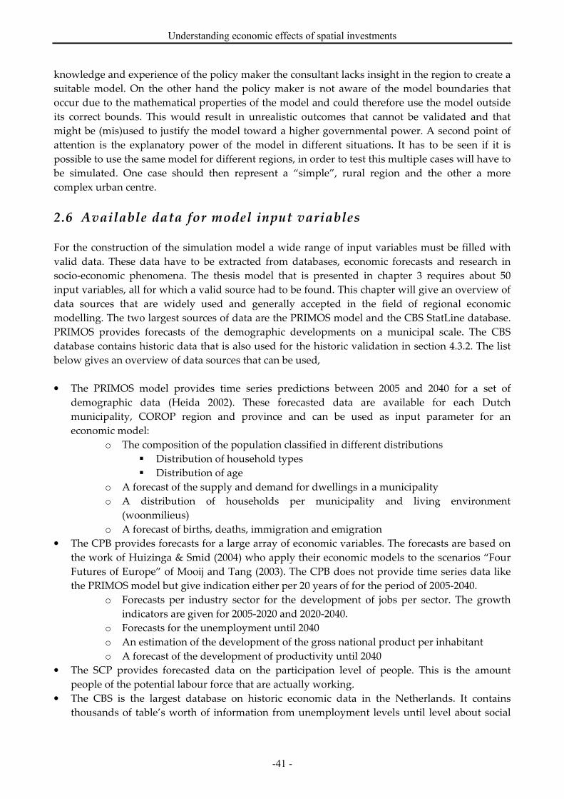
Understanding economic effects of spatial investments
-41 -
knowledge and experience of the policy maker the consultant lacks insight in the region to create a
suitable model. On the other hand the policy maker is not aware of the model boundaries that
occur due to the mathematical properties of the model and could therefore use the model outside
its correct bounds. This would result in unrealistic outcomes that cannot be validated and that
might be (mis)used to justify the model toward a higher governmental power. A second point of
attention is the explanatory power of the model in different situations. It has to be seen if it is
possible to use the same model for different regions, in order to test this multiple cases will have to
be simulated. One case should then represent a “simple”, rural region and the other a more
complex urban centre.
2.6 Available data for model input variables
For the construction of the simulation model a wide range of input variables must be filled with
valid data. These data have to be extracted from databases, economic forecasts and research in
socio-economic phenomena. The thesis model that is presented in chapter 3 requires about 50
input variables, all for which a valid source had to be found. This chapter will give an overview of
data sources that are widely used and generally accepted in the field of regional economic
modelling. The two largest sources of data are the PRIMOS model and the CBS StatLine database.
PRIMOS provides forecasts of the demographic developments on a municipal scale. The CBS
database contains historic data that is also used for the historic validation in section 4.3.2. The list
below gives an overview of data sources that can be used,
• The PRIMOS model provides time series predictions between 2005 and 2040 for a set of
demographic data (Heida 2002). These forecasted data are available for each Dutch
municipality, COROP region and province and can be used as input parameter for an
economic model:
o The composition of the population classified in different distributions
� Distribution of household types
� Distribution of age
o A forecast of the supply and demand for dwellings in a municipality
o A distribution of households per municipality and living environment
(woonmilieus)
o A forecast of births, deaths, immigration and emigration
• The CPB provides forecasts for a large array of economic variables. The forecasts are based on
the work of Huizinga & Smid (2004) who apply their economic models to the scenarios “Four
Futures of Europe” of Mooij and Tang (2003). The CPB does not provide time series data like
the PRIMOS model but give indication either per 20 years of for the period of 2005-2040.
o Forecasts per industry sector for the development of jobs per sector. The growth
indicators are given for 2005-2020 and 2020-2040.
o Forecasts for the unemployment until 2040
o An estimation of the development of the gross national product per inhabitant
o A forecast of the development of productivity until 2040
• The SCP provides forecasted data on the participation level of people. This is the amount
people of the potential labour force that are actually working.
• The CBS is the largest database on historic economic data in the Netherlands. It contains
thousands of table’s worth of information from unemployment levels until level about social

Master Thesis – Teun Veldhuizen
- 42 -
safety. The data that can be used from the CBS is either used to extrapolate data or to indicate
starting values of basic model variables. Below only the selection of data that is used in the
thesis model is illustrated24.
o The start value of: dwellings in the region, jobs per industry sector in the region,
jobs per industry national, unemployment, working labour force, labour force,
disposable income of households, average spending on daily, non-daily and leisure.
o The habitat quote
• The Locatus retail explorer (Locatus 2004) gives and indication of the demand for retail in a
region.
• The retail yearbook (HDB 2004) provides data on the size of retail per COROP area and is
updated on a yearly basis. The yearbook also gives information on different retail sectors and
the demand for retail in a region.
• The “Koopstroomonderzoek” of Goudappel Coffeng (KSO 2004) gives information on the
distribution of regional spending by inhabitants of a region.
2.7 Conclusion of model conditions and environment
In chapter 2 the first thesis sub question formed the departure point for the search for the most
important indicators and underlying relations of the instrument that has to be built. By executing
step 4, 5 and 6 the sub questions can now be answered in the conclusion of this chapter.
What are the leading indicators and underlying relations of an instrument for the ex-ante exploration and
assessment of policy options in spatial investments in a region?
a. What are the user requirements of such an instrument?
b. What can be learned and used from the existing models or instruments for regional economic
analysis?
c. What are the generally accepted data sources that can be used as input parameters for such an
instrument?
Chapter 2 started with exploring the environment where the instrument should be able to work in.
From studying the policy life cycle in chapter 2.1.2 it can be concluded that the place of the thesis
simulation model in the policy life cycle comes best to justice in the policy formulation phase. This
is supported by the intention to develop a model that is able to answer what-if questions in the
coming about of policy proposals. The geographical scale of the simulation model is the COROP
level, for COROP regions relatively much information is available. The COROP classification also
provides a fine meshed division of the Netherlands in 40 regions. Within these regions it must
however be possible to assess individual municipalities or groups of municipalities.
The requirement analysis has led to the answers of another sub question of the thesis and also
forms a basis for the simulation model construction. By interviewing policy makers, consultants
and model experts the important requirements were discovered and categorized. Some of the most
important requirements are that the model must:
• Offer different sets of complexity, some actors are interested in highly detailed information,
while others prefer a so-called “jip-and-janneke” version.
• Include the regional demographic, employment and housing market developments.
24 All the data is available online through the StatLine website: www.statline.cbs.nl

Understanding economic effects of spatial investments
-43 -
• Differentiate the production sectors in order to indicate economic and job development per
industry sector.
• Show a distribution of the uncertainty of the outcomes and the sensitivity of the input
parameters early in the policy process.
• Provide a clear indication of the assumptions that were made during the model construction.
• Show the socio-economic effects of different policy options under different economic
scenarios.
• Export the outcomes of a simulation run to an Excel file so it can be used for later analyses.
Specifically for the Wieringerrandmeer case the simulation model must show the effects of
tourism, the model must assist in quantifying the risk for both Wieringen and Wieringermeer. The
model must also be able to show the effects of stopping the project halfway.
From the requirement analysis and the research into existing economic models it can be concluded
that the three most important indicators for the socio-economic instrument are:
1) Demographic data
a. Age and household distribution
2) Employment data
a. The development of jobs in different industry sectors
3) Economic data
a. Spending in the region
b. Gross regional product
These indicators need to have a prominent place in the outcomes of the instrument that is
presented to the policy makers.
The raison d’etre of the thesis model is based on shortcomings of currently available models for
assessment of regional investment projects. These models either have a wrong geographical focus
(mostly national), they do not correctly convey the uncertainty of the outcomes or they are too
difficult to function in a dynamic group session. The current models are also quite costly (more
than €25.000) and for that price a competitive product can be developed. As stated already in the
introduction, the shortcomings of the other model leave possibilities for the system dynamics
methodology. The non-linear, dynamic and time dependent behaviour of the regional economy
also leads to this conclusion. Another and perhaps more important reason for studying other
economic models is looking at possibilities to use concepts, equations and data from these models.
• The PRIMOS model is a complex demographic projection model. It might be helpful to use the
PRIMOS time series output data as input for the model that has to be developed (Heida 2002).
Furthermore PRIMOS supplies some excellent insights in how demographic development
comes about and what motivates inhabitants of a region to migrate to another region (see
figure 2.3 and 2.4)
• The REGINA model from TNO shows that a relatively simple technique like shift-share
analysis can be extended to make it more realistic in presenting economic and labour market
developments.
• The regional labour market model from the CPB is useful because it has examined, based on
empirical data, the relationships between housing, employment and migration. These issues
are particularly important for the thesis model. The quantified relations might prove helpful
during model construction.

Master Thesis – Teun Veldhuizen
- 44 -
The third and final aspect of the first sub question concerns the data sources that are available and
accepted and that are required for the input variables of the instrument. The following most
relevant data sources have been identified:
• The PRIMOS model provides time series predictions between 2005 and 2040 for a set of
demographic data (Heida 2002). These forecasted data are available for each Dutch
municipality, COROP region and province and can be used as input parameter for an
economic model:
o The composition of the population classified in different distributions
� Distribution of household types
� Distribution of age
o A forecast of the supply and demand for dwellings in a municipality
o A distribution of households per municipality and living environment
(woonmilieus)
o A forecast of births, deaths, immigration and emigration
• The CPB provides forecasts for a large array of economic variables. The forecasts are based on
the work of Huizinga & Smid (2004) who apply their economic models to the scenarios “Four
Futures of Europe” of Mooij and Tang (2003). The CPB does not provide time series data like
the PRIMOS model but give indication either per 20 years of for the period of 2005-2040.
o Forecasts per industry sector for the development of jobs per sector. The growth
indicators are given for 2005-2020 and 2020-2040.
o Forecasts for the unemployment until 2040
o An estimation of the development of the gross national product per inhabitant
o A forecast of the development of productivity until 2040
• The CBS is the largest database on historic economic data in the Netherlands. It contains
thousands of table’s worth of information from unemployment levels until level about how
safe people feel. The data that can be used from the CBS is either used to extrapolate data or to
indicate starting values of basic model variables. Below only the selection of data that is used
in the thesis model is illustrated25.
o The start value of: dwellings in the region, jobs per industry sector in the region,
jobs per industry national, unemployment, working labour force, labour force,
disposable income of households, average spending on daily, non-daily and leisure.
o The habitat quote.
• The “Koopstroomonderzoek” of Goudappel Coffeng (KSO 2004) gives information on the
distribution of regional spending by inhabitants of a region.
25 All the data is available online through the StatLine website: www.statline.cbs.nl

Understanding economic effects of spatial investments
-45 -
3 Model construction
In this third chapter the second sub question of the thesis forms the basis of the research. Now the
preliminary phases have been executed the real model building can start. As step 7 the economic
relations will be explored first based on the knowledge from the requirement analysis and the
study of literature and existing models. Then as a step between the actual model and the
requirement analysis a concept model needs to be developed. Chapter 3 thus shows two
transformations; first the results from the requirement analysis, the exploration of economic
relations and literature study are transformed in the concept model. The second transformation is
that of the concept model in the actual mathematical model. The key assumptions and decisions of
the design process are worked out in detail and the SD theory is tested on its applicability in the
final model.
How to construct an instrument for the ex-ante exploration and assessment of policy options in spatial
investments in a region?
a. How are the notions from the requirement analysis, literature study and existing models translated
into a conceptual model?
b. How is this conceptual model translated into a mathematical simulation model?
The leading indicators identified in the previous chapter and the theoretical framework form the
starting point for the design of the concept model. In section 3.1 the general concept is given, basic
decisions and assumptions are explained. Section 3.2 deals with the causal and empirical
relationships that appear in the concept model. Then in section 3.3 the transformation of the
concept model into the final simulation model is described. The assumptions that were made
during the complete design process are described in section 3.4 and the model specifications can be
found in 3.5. An aspect that is placed high on the list of user requirements is the interface, how the
interface communicates with the model user is described in section 3.6. And finally in 3.7 the
conclusion is given based on the insights gained during the development of the simulation model.
3.1 The simulation model concept
The simulation model must provide insight in the socio-economic developments that will take
place in a certain region; the region in this case is a set of municipalities within a COROP area. A
requirement states that for this region the model must be able to calculate different scenarios, both
economic and policy scenarios. The policy scenario discloses the available policy options and
external policy events; for instance the delay of the investment project. The economic scenario
illustrates the effects on the project region of either a growing or declining economy. The economic
scenarios are based on the commonly used CPB scenarios (Huizinga & Smid 2004). The case in
which the investment project is not executed is called the autonomous policy scenario; it illustrates
Chapter 3: model construction
8)Develop
conceptual model
9)Develop
simulation model
7)Explore
economic relations
Subquestion 2

Master Thesis – Teun Veldhuizen
- 46 -
the effect of the base case or 0-option. The impulse policy scenario gives an indication of the socio-
economic effects in the region when the investment is made. The effects in the impulse scenario
illustrate also if the project requirements are met and if the desired political goal is reached. Figure
3.1 is taken from the simulation model and illustrates the development of jobs in the region over a
period of 25 years. The impulse scenario is presented in pink against the autonomous scenario in
blue. The striped section between the lines indicates the extra jobs created by the investment
project. Having a visual representation of the economic effects is another model requirement.
Figure 3.1, jobs in the autonomous (blue) and impulse (pink) scenario
The general concept of the simulation model is that it combines theoretical relationships found in
system dynamics with empirical data from other models and prognoses. Why this combination is
necessary is explained in the following section. The input data, or data that is required to run the
model comes from a variety of sources. The CPB delivers economic forecasts in the form of growth
percentages, the SCP provides participation levels in the workforce, and demographic data comes
from the PRIMOS model etcetera. To comply with the model requirements the key input factors of
the model are (see figure 3.2):
Figure 3.2, the core variables of the simulation model and the important in- and outputs
1 ja n 2 00 5 1 ja n 2 0 10 1 ja n 20 1 5 1 ja n 2 02 0 1 ja n 2 0 25 1 ja n 20 3 0
5 .5 0 0
6 .0 0 0
Ba a n
Non-com m ercia l us e on ly!
cv
Predicted housing supply(2005 -2030)
Investment impulse (2005-2030)
Housing supply (2005-2030)
CPB scenarios (2005-2030)
Employment data (2005)
Gross regional product(2005)
Jobs (2005)
Predicted demographics (2005 -2030)
Regional income (2005-2030)
Jobs (2005-2030)
Gross regional product (2005-2030)
Demographics (2005-2030)
Inhabitants
Dwellings
Jobs
Regional
income
Data input Simulation model Data output
Understanding economic effects of spatial investments
-47 -
• The predicted housing supply and demographics by PRIMOS. The demographic data consists
of inhabitants in age groups and household types.
• The CPB economic scenarios for the Netherlands until 2040 (Huizinga & Smid 2004), in the
model only used until 2030.
• Data that describes the current situation: the jobs in different industry sectors, regional income
and regional productivity.
• The proposed investment project that is translated into a growth in the number of houses and
facilities in the project region.
• The present supply of recreational and other facilities to comply with the requirements from
the case study Wieringerrandmeer.
The four most important simulation model variables are the number of dwellings (houses) in the
project region, the inhabitants, the regional income and the development of jobs in different
industry sectors. The data generated by the model is exported to MS Excel spreadsheets for
analysis and further processing. The output of the model is focused on the regional socio-economic
factors and is in correspondence to the requirements from step 4:
• The total housing supply including the investment impulse until 2030.
• Developments of demographic variables (households types and age groups) until 2030.
• The development of the gross regional product until 2030.
• The jobs per industry sector in the project region until 2030.
• Developments in the regional income and spending in the region until 2030.
3.1.1 Using exogenous data to keep the model manageable
Initially Forrester’s Urban Dynamics model was intended as the basis of the thesis simulation
model (see section 2.4.1). The Urban Dynamics model however is a completely theoretical model
without empirical data (Garn 1972); this means that most of the variables in Forrester’s model are
endogenous. A completely endogenous model would also require the development of a
demographic and labour market model component. Looking at the size, complexity and quality of
existing demographic models like PRIMOS it is almost impossible to replicate such a model in a
system dynamics environment. A model of such complexity would compromise the requirement
to develop a manageable model and would furthermore exceed the given time for this thesis
project. This leaves the option of using the time series projections of PRIMOS as input for the
model. There are more indications that using external data is better than developing an
endogenous model that does not inhibit the properties of Forrester’s UD model:
• First, if only theoretical assumptions constitute the model the description of for instance the
demographic developments require a far more complex model. This complexity would
contravene the goal of the thesis model to be comprehensible and manageable. Through the
introduction of empirical data from existing models the complexity of the model can be kept
within limits.
• The second argument for not only using theoretical relations is the relevance of the information
that has to be presented towards the end user, the policy maker. The Urban Dynamics model
has never been validated on an empirical case and would be hard to ex-ante verify the
correctness on an actual situation. The actual data derived from the Wieringerrandmeer case
study cannot be implemented in the UD model. The outcomes of the UD model do not comply
with the user requirements. For instance, it is not possible in the UD model to attribute

Master Thesis – Teun Veldhuizen
- 48 -
different industry sectors, neither is it possible to give insight in demographic effects like age
or household distribution.
Using the urban dynamics model as starting point for the thesis model becomes impossible if the
user requirements are to be met. There are two more arguments for not using UD that give the
decisive proof.
• The time span of the UD model exceed by 10 fold the intended time span of the thesis model
(Forrester 1969). Forrester’s model describes the growth of a small town that, over a period of
250 years evolves to a major metropolis (see also figure 2.7). The time span for the thesis is only
25 years.
• Finally, the geographical scale of Forrester’s model is that of one urban area, a small town,
which grows to be a large metropolis over a period of 250 years. The geographical scale that is
required for the thesis model is that of several smaller municipalities and the using data from
COROP regions.
Does this then mean that all the theoretical concepts of the UD model will have to be abandoned?
No, some key concepts of the urban dynamics model can be used in the concept model. For
instance the concept that disposable income can be deducted from the quality (in this case price) of
a house. This concept is used in the simulation model to estimate the disposable income of the new
inhabitants of the project region. Also the concepts of attractiveness of a region remain important
for the construction of the model.
A mentioned before, causal feedback loops are one of the major properties of system dynamics.
The concept model presented in figure 3.3 does however not show any causal feedback loops. The
question then comes to mind if the concept model is a true system dynamic model? All the other
conditions surrounding the problem and the development of the model are evidence of and
approve of the use of system dynamics. The model’s properties (time dependent, dynamic and
non-linear) all justify the use of system dynamics. Why the feedback loops are not present in the
concept model can be explained by the exogenous data itself. The exogenous data “breaks up” the
feedback loops in the system. More attention is given to this subject in section 5.1.
3.2 Cause-and-effect relationships as basis for the concept model
The causal relationships in the concept model form the basis for the design of the simulation
model. Figure 3.3 depicts this basic causal model. The “Housing impulse” and “Leisure impulse”
are the steering variables where that determine the policy plan. The impulse variables will
influence the entire system over time as each variable is connected to the economic system in the
simulation model. The remainder of this section provides an overview of all the individual
relations. The numbers on the relationships lines correspond to the descriptions that are summed
up in the remainder of this section. The numbers inside the ellipse shaped variables in figure 3.3
indicate the source of data that is used as input for that particular variable. De numbers
correspond respectively to:
1) PRIMOS model data
2) Data from the Social and Cultural Planning Office of the Netherlands (SCP)
3) Base data for shift-share analysis stems from Statistics Netherlands (CBS)
4) Different sources (Locatus, Detail Handel Jaarboek, Koopstroomonderzoek)
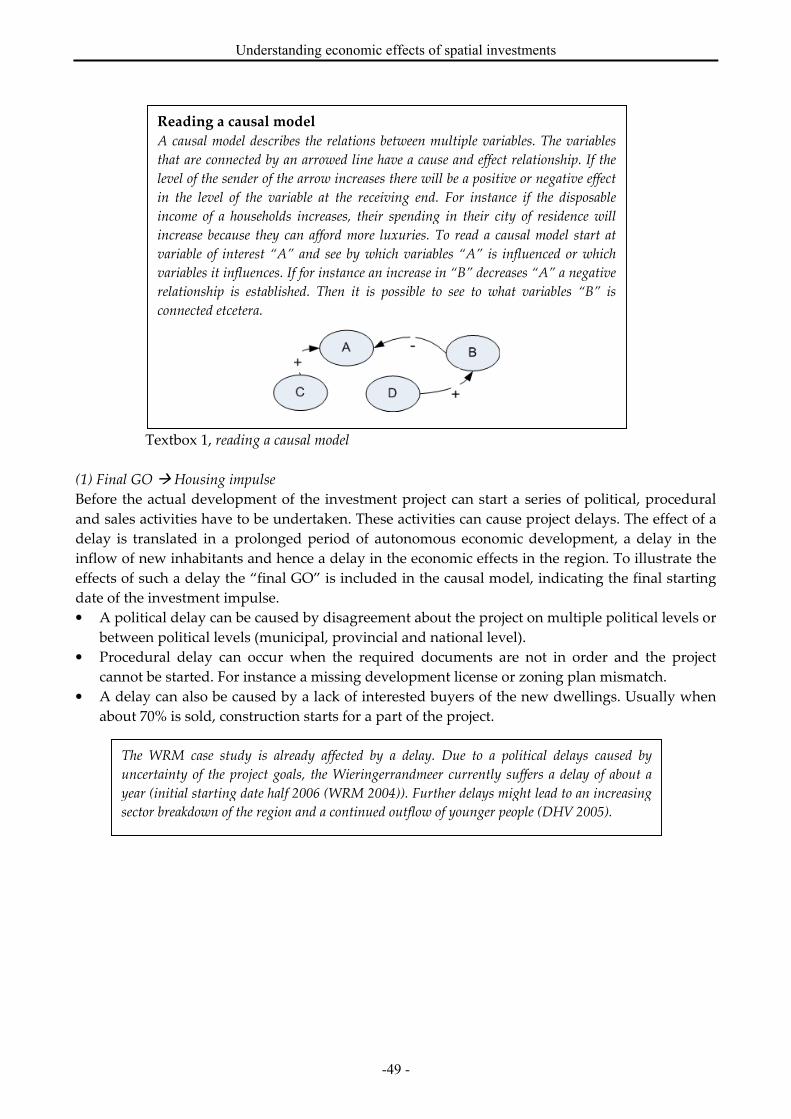
Understanding economic effects of spatial investments
-49 -
Textbox 1, reading a causal model
(1) Final GO � Housing impulse
Before the actual development of the investment project can start a series of political, procedural
and sales activities have to be undertaken. These activities can cause project delays. The effect of a
delay is translated in a prolonged period of autonomous economic development, a delay in the
inflow of new inhabitants and hence a delay in the economic effects in the region. To illustrate the
effects of such a delay the “final GO” is included in the causal model, indicating the final starting
date of the investment impulse.
• A political delay can be caused by disagreement about the project on multiple political levels or
between political levels (municipal, provincial and national level).
• Procedural delay can occur when the required documents are not in order and the project
cannot be started. For instance a missing development license or zoning plan mismatch.
• A delay can also be caused by a lack of interested buyers of the new dwellings. Usually when
about 70% is sold, construction starts for a part of the project.
Reading a causal model
A causal model describes the relations between multiple variables. The variables
that are connected by an arrowed line have a cause and effect relationship. If the
level of the sender of the arrow increases there will be a positive or negative effect
in the level of the variable at the receiving end. For instance if the disposable
income of a households increases, their spending in their city of residence will
increase because they can afford more luxuries. To read a causal model start at
variable of interest “A” and see by which variables “A” is influenced or which
variables it influences. If for instance an increase in “B” decreases “A” a negative
relationship is established. Then it is possible to see to what variables “B” is
connected etcetera.
The WRM case study is already affected by a delay. Due to a political delays caused by
uncertainty of the project goals, the Wieringerrandmeer currently suffers a delay of about a
year (initial starting date half 2006 (WRM 2004)). Further delays might lead to an increasing
sector breakdown of the region and a continued outflow of younger people (DHV 2005).

Master Thesis – Teun Veldhuizen
- 50 -
Figure 3.3, concept causal model
(2) Housing impulse� Dwellings
The housing impulse starts the construction of the dwellings in the region. Through a delay that
compensates for the building time the number of dwellings increases directly the number of
dwellings in the project region.
Facilities and services (4)
Medical care Retail Leisure
# Dwellings (1)
Productivity
Gross added value (3)
# Jobs (3)Regional disposable income (3)
+ (17)
# Inhabitants (1)
Regional potential
labour force
Regional labour force
+ (21)
+ (23)
Regional working labour
force
Gross participation
(2)
+ (22)
- (25)
Unemployment (nett
participation)
+ (24)
+ (6)
+ (18)
Housing impulse
(1)
+(2) + (4)
+ (3)
Disposable income new inhabitants
Spending in region
+ (10)
+ (8)
Portion regional spending
+ (12)
+ (5)
+ (15)+ (14)
+ (11)
Leisure impulse
+ (16)
Tourism spending
+ (13)
+ (19)Disposable income per household (3)
+ (9)
+ (20)
# Households (1)
+ (26)
Housing reservation
+ (7)
Understanding economic effects of spatial investments
-51 -
(3) Housing impulse � Disposable income new inhabitants
An attribute of the housing impulse is the average price of the new dwellings in the project region.
The disposable income of the new inhabitants of the project dwellings will be proportional to the
average house price of the project. This is based on the assumption that people spend on average
the same percentage of their disposable income on the costs of housing. Using the average housing
price, the mortgage and “woonquote26” the disposable income of the new inhabitants can be
estimated. In general this means that if the prices of dwellings are higher the disposable income of
the inhabitants is higher. (CBS StatLine: woonuitgaven 1990 - 2000)
(4) Dwellings � Households
There is a one on one relationship between the number of dwellings and the number of households
because a new household occupies each new dwelling. The households are divided into four basic
household settings (CBS compliant):
• Single parents
• Living together with kids
• Living together no kids
• Living alone
This distribution of the types of households of the new inhabitants can be determined in two ways.
Either beforehand, during the input of new data into the simulation model or the new household
distribution is similar to the current household distribution.
(5) Dwellings � Inhabitants
The development of inhabitants in the project area is controlled by two variables. The first variable
is controlled by the PRIMOS forecasts and provides a null-scenario, hence the autonomous growth
of inhabitants in the region (Heida 2002). The second variable controls the inhabitants of the newly
26 Woonquote: the total costs of housing (including municipal charges and public utility expenses) expressed
as percentage of the disposable income.
The situation in the WRM region is such that the newly build project dwellings have a higher
value than the existing dwellings currently present in the region. This means that the new
inhabitants have a higher disposable income, hence more spending in the region, which in
turns results in an improved regional economy.
A strong increase in the number of single households can be observed in the Netherlands. The
WRM project region is subject to an increased effect of single household increase due to the
over performance of aging in the region compared to the Netherlands. The WRM housing
project is partly aimed at reducing the level of single households and lowering the aging rate.
The WRM project consists of four building phases, each of these phases delivers a set of
dwellings with a grand total of 1845 dwellings (Lago Wirense 2004):
Phase 1: 150 dwellings over a period of 5 years
Phase 2: 355 dwellings over a period of 6 years
Phase 3: 760 dwellings over a period of 5 years
Phase 4: 580 dwellings over a period of 9 years

Master Thesis – Teun Veldhuizen
- 52 -
built project dwellings. By multiplying the average household size of the new households with the
number of households the amount of new inhabitants is calculated. The inhabitants grow
according to an age distribution in four age groups (PRIMOS compliant):
• 0 – 14 years old
• 15 – 29 years old
• Lago Wirense (2004). 30 – 64 years old
• 65 and older
Just like the distribution of household types the distribution of age of new inhabitants will either
be appointed during the input of new data into the simulation model or be similar to the current
age distribution.
(6) Inhabitants � Regional potential labour force
A selection of the inhabitants based on age belongs to the potential labour force. Using the
distributions from the age groups the inhabitants between 15 and 65 years of age make up the
regional potential labour force (CBS compliant).
(7)(9) Households and disposable income per household (of current inhabitants)� Regional disposable
income
In order to obtain the value of the regional disposable income the number of households in the
region is multiplied with the disposable income per household. The regional disposable income
controls part of the spending in the project region, which in turn influences the facilities and
services. The data from the disposable income per household is derived from the CBS StatLine
website.
(8) Disposable income per new household � Regional disposable income
The disposable income of the new residents in the project region is calculated separately from the
disposable income of the existing residents (relation 9). If the dwellings of the WRM project are
more expensive compared to the existing dwellings, the disposable income of the new inhabitants
will also be higher (see also relation 3). This effect is explained in more detail in section 3.3.3.
The current predictions for the WRM forecast a fast growing elderly population (faster than
national) and a reduction of births and therefore young people. In general the population will
shrink in the WRM area. In the end this causes the foundation for services and facilities to
diminished and gradually dissolve. The WRM project aims at reducing the rate of aging and
shrinking of population in the project region.
The effect of the increasing aging population in the WRM region leads to a decrease in the
people in the regional potential labour force. A reduction of the potential labour force will lead
to a reduced growth of jobs in the region.
The current level of disposable income per year is € 30.500 per household, which lies above
the national average (CBS StatLine)! However the total disposable income in the WRM
region is currently at a sustainable level but diminishes significantly the coming 20 years
(DHV 2005).

Understanding economic effects of spatial investments
-53 -
(10)(12) Portion regional spending & Regional disposable income� Spending in Region
Households do not spend all their disposable income in their home region or municipality. For
instance, when an inhabitant of a rural town needs to purchase non-daily products (furniture,
electronic appliances etcetera) he or she has to go to a larger, more urban city to find a furniture or
electronics store (Koopstroomonderzoek Randstad 2004). This means that if an area is more rural, a
smaller portion of the disposable income is spent in the region. The opposite holds for inhabitants
of large urban regions. They do not have to go to other regions for non-daily purchases, simply
because the supply of non-daily products in their home region is sufficient. To correct this effect in
the concept model the portion of regional spending is a percentage of disposable income spent in
the home region. Because the rate of regional binding is different for different types of products
three sources of spending are identified in the simulation model (Koopstroomonderzoek Randstad
2004):
• Daily spending: Grocery stores, small clothing stores.
• Non-daily spending: Electronic-, Hardware-, Furniture-, specialized clothing stores
• Leisure spending: Daytrips, spending in bars, restaurants
(11)(19) Inhabitants � healthcare� Jobs
A direct effect from the increase in residents is the additional need for healthcare services and
facilities and hence healthcare jobs. This makes the healthcare services a non-basic sector,
controlled directly by the healthcare demand from the inhabitants (Armstrong 1993). This non-
basic effect is not calculated through the shift-share analysis. In stead, the average employment in
healthcare services per inhabitant is multiplied with the number of new inhabitants and added to
the present level of jobs in healthcare (A more detailed description in section 3.3.1).
The public administration of the WRM region fears that the combination of an aging
population and the decrease of younger people in the region will further reduce the foundation
for professional healthcare services. They argue that this will lead to a further decrease of
population in the region (from meeting with Lago Wirense Project Management Team in
October 2005).
Currently only estimations can be made on the price of the new dwellings in the WRM
project. The latest estimation is an average price of €300.000 per dwelling (meeting with
Arjan Stegeman 11-05-2006) which leads to an disposable income of €48.000 per household
(with “woonquote”: 25% and interest rate: 4%. However a more detailed market study should
be performed in order to get a more precise indicator of the average dwelling price.
The WRM region can be classified as rural and therefore has a relative small regional binding
factor. For the daily spending 85% is spent in the region, for non-daily this is 40% and for
leisure 30%. By increasing the amount of inhabitants and amenities in the region the binding
factor will increase as inhabitants do not have to go to other regions for their groceries and
other purchases.

Master Thesis – Teun Veldhuizen
- 54 -
(13) Tourism spending � Spending in region
An increased impulse of tourism will lead to higher tourist spending in the region. Tourist
spending is allocated in two sectors: the hotel and restaurant sector (sub sector of commercial
services) and the trade sector. An increase of tourist spending must be preceded by an investment
in tourist facilities (hotel, restaurant, boat rental etcetera).
(14) Spending in region� Facilities and services / Retail
When the spending in the region increases as a cause of more regional disposable income, higher
regional binding or higher tourist spending the foundation for retail and leisure facilities also
increases. The Dutch board for retail trade (Hoofdbedrijfschap detailhandel) and Locatus27 provide
data for the effects of higher spending in the region on the level of services. When commercial and
non-commercial services in the region increase the jobs in those sectors will also increase (relation
19).
(15) Spending in the region � Facilities and services / Leisure
(16) Leisure impulse � Leisure
Like relation 14, more spending in the region increases the level of services and facilities of for
leisure. Extra disposable income in the region as a result of new inhabitants has a direct effect on
the available space for leisure facilities. The Dutch board for retail trade (HBD) and Locatus
provide data for the effects of extra inhabitants on both the level of leisure activities in a region as
the added effect for the employment in the region. When the investment project is executed new
leisure will be developed which is expressed in square meter of working accommodation.
(17)(18) Jobs and Productivity � Gross regional product
Productivity indicates the sector specific added value per employee in a region (data from CBS
StatLine). When the productivity is multiplied with the current jobs in the region the gross
regional product can be derived. The gross regional product or regional income is an important
indicator for the economic health of a region. When the regional product diminishes the indicator
is often a decreasing amount of jobs or an increase of jobs with a lower added value (lower
productivity) (Armstrong 1993). Note that the jobs in the region do not necessary have to be
27 Locatus: company supplying retail trade, services and hotel and catering industry information
An important aspect of the WRM project is increasing the tourist attractiveness of the region.
The new lake is supposed to attract different water sport activities like sailing, fishing and
beach tourism. The environment around the lake will be equipped with cycling- and footpaths
to attract nature tourism. The supply of hotel and camping facilities will also be expanded
(Lago Wirense 2004). Currently the income from tourism is less then 1% (DHV 2005).
The supply of a (large) range of retail facilities is important for the attractiveness of the WRM
region, both for inhabitants as for tourists (VNG 2006). The WRM project strives to increase
the spending in the region by increasing the level of retail facilities. Attracting more
inhabitants through the housing project and more tourists by developing new facilities around
the lake.
Currently tourism and leisure facilities in the WRM region are almost negligible, therefore
spending by both tourists and local inhabitants is very limited. The WRM project causes a
leisure impulse that is supposed to kick-start the leisure facilities in the project region.

Understanding economic effects of spatial investments
-55 -
fulfilled by the inhabitants of the region this separates the spending income of the region from the
gross added value.
(19) Facilities and services / Leisure and Retail � Jobs
The level of services and facilities of leisure and retail is calculated in square meters of working
accommodation per sector (square meter floor space). The HDB specifies ratios of employees per
square meter for the leisure and retail industry (HDB 2005). Using these ratios and floor space
area’s the employees in these sectors can be calculated. Spending in the region will lead to an
increase in square meter floor space, which in turn will lead to an increase in jobs through the
employee per square meter ratio.
(20) Potential labour force � Jobs
The relation between potential labour force and the jobs in a region has been disputed over time.
There are two theories that support both directions of the causality between potential labour force
and jobs (see also section 2.3.3). The paradigm is that either people-follow-jobs or jobs-follow-
people.
• Jobs � Potential labour force: this directionality can be theoretically funded by assumptions that
migrants come into a region when wages in that region are higher compared to adjacent
regions. The economic agglomerations effects will (in this line of thought) drive up wage levels
as employment becomes scarcer. The higher wages in the region will attract people to the
region that eventually will settle in the region. Hence, people follow jobs.
• Potential labour force � Jobs: supporters of jobs follow people make the point that people do not
move to other areas for higher wages but for more and better amenities. The amenities are in
that case the most important factor in population growth. The people that move to high
amenity locations demand consumer goods and supply labour. In turn the people that move to
a region supply labour that attracts firms, hence, jobs follow people (Vermeulen & van
Ommeren 2005, pp. 3). In the thesis model the latter relation is used: jobs-follow-people
because it is more accepted than people follow jobs. Vermeulen and van Ommeren (2005) proof
in their paper that jobs follow people.
The WRM currently has a small range of leisure facilities, most of them being bars and small
hotels (SCBA Lago Wirense 2006). These facilities make up less then 2 % of the total jobs in
the region. Under the WRM project the jobs in these sectors can increase more then 5 %
(DHV 2005).
The gross added value of the WRM region has the potential to increase with 20% if the project
is executed. The WRM region does cope with a relative low productivity compared to the
Dutch average. This is mainly due to the high portion of jobs in the primary sector where
added value per job is lower compared to other sectors (DHV 2005).
The growth of jobs in the WRM region is currently based on the historic performance of the
production sectors in the region. However over time, using the jobs-follow-people principle,
the job development will partly be determined by the availability of labour.

Master Thesis – Teun Veldhuizen
- 56 -
(21..25) Inhabitants and labour force
Some of the relationships in the concept model are standardized and come directly from other
models. Figure 3.4 shows the deduction of the working labour force from the total inhabitants of a
region. Only a part of the inhabitants belongs to the
potential labour force, these people are of working age (15
to 65 years old) this classification is also used by Statistics
Netherlands. Because not every person in the potential
labour force is working the gross participation28 indicates
which percentage of the potential labour force is actually
working or looking for work. The former and the latter
combined make up the labour force, the inhabitants of a
region that have a job are grouped in the bottom category
of figure 3.4; the working labour force. These indicators
together illustrate the amount of inhabitants that are
currently working, unemployed or not of working age.
The indicators do not however give information about the
jobs that are available in the region. The inhabitants that
are part of the working labour force could work outside of
the region and not contribute to regional employment.
Figure 3.4, labour force
3.3 Translation of the concept- into the simulation model
Section 3.3 describes the translation of the concept model into the quantified simulation model.
This translation is actually a sophistication of the concept model. The relations presented in section
3.2 are often not as simply implemented as presented in the concept model. This section therefore
elaborates on the relations as they have been implemented in the simulation model. Section 3.3
describes the specific implementation of the concept model in the software programs PowerSim
and Microsoft Excel. The simulation model is presented in set of 11 sub-models in figure 3.5. The
sub models fall into three categories and will be discussed accordingly.
1. Labour market developments in the basic and non-basic industry sectors
2. Regional spending and disposable income
3. Inhabitants and available labour force developments
The tripartite division of the model will also be used in the discussion of the model assumptions in
section 3.4 and in the sensitivity analysis in section 4.2.
28 Participation level data available through the Social and Cultural Planning Office of the Netherlands
(SCP). Historical data available on a COROP level, predicted values available only on national level.
Inhabitants
Potential labour force
Labour force
Working labour force
Inhabitants of
working age
Gross
participation
UnemploymentNet
participation
Inhabitants to Working labour
force
The current age distribution in the region is fairly equal to the national average with a slightly
older population. This results in a potential labour force that comprises of 67% of the total
population. The forecasts show a decrease of potential labour force compared to the national
average, which indicates economic decline over a longer period (DHV 2005).

Understanding economic effects of spatial investments
-57 -
Figure 3.5, components of the simulation model
The sub models are described and discussed in more detail in the rest of this section. Special
attention is given to relations that are not worked out in detail in the concept model of figure 3.3.
Section 3.3.1: Labour market developments in the basic and non-basic industry sectors
• Figure 3.6: shift share analysis in PowerSim. This is the calculation of the job development in
the basic sectors in the project region.
• Figure 3.8: the healthcare sector developments of a non-basic sector and the influence on the
job development in the project region
• Figure 3.9: the retail sector developments (non-basic sector) and the influence on the job
development in the project region
Section 3.3.2: Regional spending and disposable income
• Figure 3.10: the summarized spending in the region (daily, non-daily, leisure and tourism
sector).
• Figure 3.11: detailed description of the tourist spending in the project region
• Figure 3.12: the deduction of disposable income of inhabitants of the project dwellings
Section 3.3.3: Inhabitants and available labour force developments
• Figure 3.13: the inhabitants and labour force in PowerSim
Section 3.3.3
Development of dwellings
Section 3.3.1
Non-basic sector development: horeca sector
Section 3.3.1
Non-basic sector development: retail sector
Section 3.3.1
Employment total and gross regional product
Section 3.3.2
Development of tourism and tourist spending
Section 3.3.1
Basic sector employment development (shift-share analysis)
Section 3.3.2
Regional spendingSection 3.3.3
Development of ouseholds
Section 3.3.3
Development of inhabitants and labour force
Section 3.3.1
Non-basic sector development: healthcare sector
Section 3.3.2
Calculation of disposable income of new inhabitants
New dwellings Basic sector jobs
Healthcare jobs
Retailjobs
Horeca jobsTourist spending
Available labour
DisposableIncome new Inhabitants
Households
New inhabitants
Inhabitants and labour force developments
Labour market
developments in the
basic and non-basic
industry sectors
Regional spending and disposable income

Master Thesis – Teun Veldhuizen
- 58 -
Text, reading a powersim diagram
3.3.1 The labour market development in basic and non-basic industry sectors
The development of jobs in a region is different for basic and non-basic sectors. Furthermore, the
entire labour market is too complex for a simple one on one relationship that increases jobs along
the increase of inhabitants in the region. Jobs in the non-basic sectors do develop as a direct
consequence of and in- or decrease of the population. While the basic sectors developed lagged
over time and are more dependent of the economic developments (Armstrong 1993) and the
availability of labour. These effects have to be incorporated in the simulation model. After long
discussion the shift-share analysis was chosen as basic modelling tool for the development of jobs
in the basic sectors (see also appendix 7). Shift-share analysis is chosen because it is relatively easy
to use and understand. This appeals to the requirements that the simulation model must be easy to
understand and reduce complexity as much as possible. Furthermore a fairly little amount of data
needed to make the shift-share calculation. The decisive factor to use shift-share analysis comes
from Koops (2005) who demonstrates with the REGINA model that it is possible to use multiple
variables to explain the development of jobs in a region. With this functionality it is possible to
include the effect of jobs-follow-people from Vermeulen & van Ommeren (2005, 2006). Shift-share
analysis extrapolates growth in production sectors through a shift and a share part (Koops 2005,
Armstrong 1993). The share part consists of the national growth indicators predicted by the CPB.
The shift part consists of multiple variables with historical performance and available labour force
as most important indicators. For the shift-share analysis the regional performance is matched to
the predicted national performance. If the shift indicators outperform the national indicators the
region will develop proportionately faster than the nation. For the non-basic sectors another
solution has been tailored to accommodate a more direct link with the growth of the population.
These relationships are illustrated in figure 3.8 and 3.9 and will be dealt with later.
Reading a PowerSim diagram
PowerSim is a system dynamics modelling program. It allows the user to
implement simple and complex causal relations in a relatively simple fashion.
There are four basic building blocks used in PowerSim (called the Stella notation).
Each of the blocks will be described shortly to help understand PowerSim
diagrams. The diamond shape on the left in the figure below indicates a static
model variable or constant. These are used to input data that does not change over
time. In this case the “RetailConstant” is linked to “RetailJobGrowth” which
controls the increase or decrease of retail jobs (this is called a rate). The large arrow
passing “RetailJobsGrowth” indicates that it is controlling the in and outflow of the
stock of “RetailJobs”. This stock variable indicates the total amount of jobs currently
active in the retail sector. The stock value of “RetailJobs” is linked by again a small
arrow to “TotalJobs” which indicates the total amount of jobs currently taken. The
last block is called an auxiliary variable and it is used to calculate values that
change over time.
RetailJobs TotalJobs
RetailJobGrowht
RetailConstant

Understanding economic effects of spatial investments
-59 -
Basic sector employment development
Figure 3.6 illustrates the implementation of the shift-share analysis in PowerSim. As mentioned
there are three basic ingredients (1 to 3) for calculating the shift share factor (4):
1) The first ingredient is the standardized shift factor that illustrates the performance of the
region with respect to the available labour force according to the jobs-follow-people principle
(Vermeulen & van Ommeren 2005, 2006). This part of the shift factor is calculated by
comparing the national ratio inhabitants per jobs to the regional ratio of inhabitants per job.
The two ratios translate either into a positive factor (over performance, the project region has
a relatively large supply of available labour and is therefore more attractive) or negative
factor (under performance, the project region has a relatively small supply of available
labour). This variable (“shift factor labour force”) then has to be standardized to become
usable in the simulation model. If the variable would not be standardized interpretation
errors can occur in the extrapolation of the historic data (Nijkamp & Reggiani 1998). Major,
one time events in the past may have had a large effect on the historic growth. Extrapolating
this growth without indication of such an event happening again would be unjust and
therefore growth (and decline) bounds should prevent excessive growth. The
standardization occurs by assigning a maximal and minimal value of the shift factor and
normalizing the old value to prevent erratic data output when approaching zero. The
maximal and minimal values that are set to the over and under performance are respectively
plus and minus one time the standard deviation of the national job growth in the
Netherlands (CBS 2005).
2) The historic performance of the region is deducted from CBS data from time period 1993–
2004. The historic performance is measured, just as labour factor above (1), relative to the
national performance. The 1993-2004 period is chosen because in 1993 the production sectors
were regrouped into the current sector division and the most recent data is from 200429.
Figure 3.6, shift-share processing in PowerSim
29 2005 data will become available later in 2006 (CBS StatLine website)
Shift-share processing
Standardization
1
2
3
4
#
Shift factor labourforce
Total regional jobs National jobs
PotBBNat
Upper limit
Lower limit
Max effect
Min effect
Shift factor labourforce standardized
Region factorNational factor
Regional historicover performance
Shift factor total
ShiftShareFactor
Job developmentCPB scenario
Historic growtheffect
NatJobGrowth
To jobs in the region
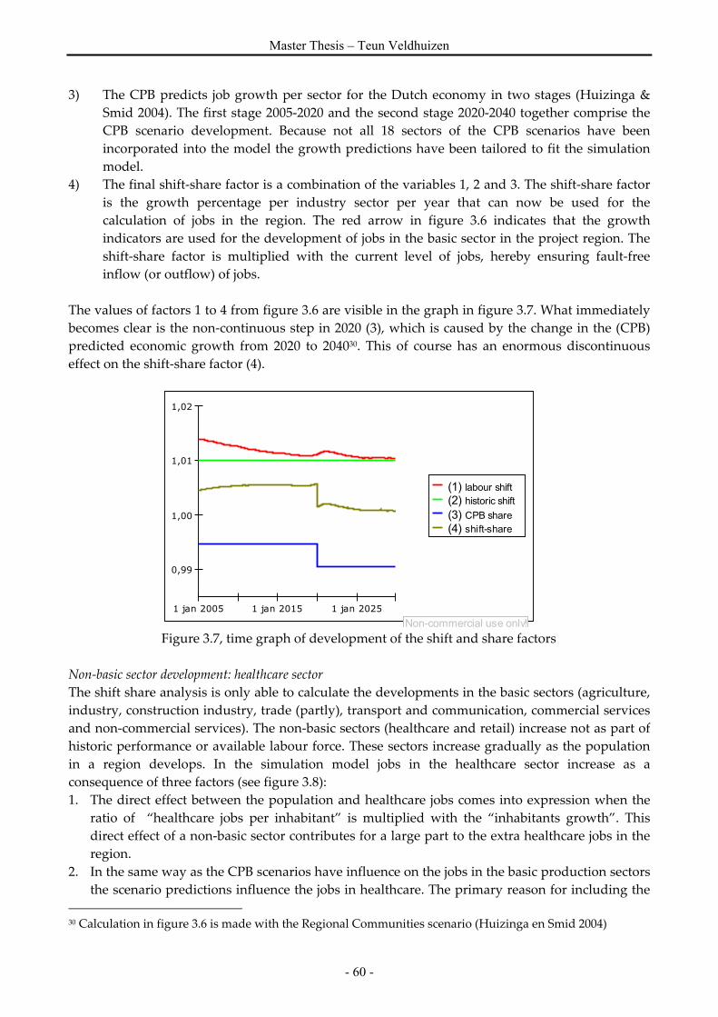
Master Thesis – Teun Veldhuizen
- 60 -
3) The CPB predicts job growth per sector for the Dutch economy in two stages (Huizinga &
Smid 2004). The first stage 2005-2020 and the second stage 2020-2040 together comprise the
CPB scenario development. Because not all 18 sectors of the CPB scenarios have been
incorporated into the model the growth predictions have been tailored to fit the simulation
model.
4) The final shift-share factor is a combination of the variables 1, 2 and 3. The shift-share factor
is the growth percentage per industry sector per year that can now be used for the
calculation of jobs in the region. The red arrow in figure 3.6 indicates that the growth
indicators are used for the development of jobs in the basic sector in the project region. The
shift-share factor is multiplied with the current level of jobs, hereby ensuring fault-free
inflow (or outflow) of jobs.
The values of factors 1 to 4 from figure 3.6 are visible in the graph in figure 3.7. What immediately
becomes clear is the non-continuous step in 2020 (3), which is caused by the change in the (CPB)
predicted economic growth from 2020 to 204030. This of course has an enormous discontinuous
effect on the shift-share factor (4).
Figure 3.7, time graph of development of the shift and share factors
Non-basic sector development: healthcare sector
The shift share analysis is only able to calculate the developments in the basic sectors (agriculture,
industry, construction industry, trade (partly), transport and communication, commercial services
and non-commercial services). The non-basic sectors (healthcare and retail) increase not as part of
historic performance or available labour force. These sectors increase gradually as the population
in a region develops. In the simulation model jobs in the healthcare sector increase as a
consequence of three factors (see figure 3.8):
1. The direct effect between the population and healthcare jobs comes into expression when the
ratio of “healthcare jobs per inhabitant” is multiplied with the “inhabitants growth”. This
direct effect of a non-basic sector contributes for a large part to the extra healthcare jobs in the
region.
2. In the same way as the CPB scenarios have influence on the jobs in the basic production sectors
the scenario predictions influence the jobs in healthcare. The primary reason for including the
30 Calculation in figure 3.6 is made with the Regional Communities scenario (Huizinga en Smid 2004)
1 jan 2005 1 jan 2015 1 jan 2025
0,99
1,00
1,01
1,02
PotBBShiftStand
Auxiliary_1
Auxiliary_2
Auxiliary_3
Non-commercial use only!
(1) labour shift(2) historic shift(3) CPB share(4) shift-share

Understanding economic effects of spatial investments
-61 -
CPB scenarios is that they consider the effect the aging population has on the demand for
healthcare jobs (Huizinga en Smid 2004). These jobs will grow more than the economy’s
average because the population keeps becoming older hence requiring more medical
attention31
3. Because the Socio-economic Effect Study (DHV 2005) illustrated that the population ages faster
in the WRM region compared to the Dutch average a “Grey pressure performance” variable
has been included. This variable corrects the healthcare jobs if the percentage persons older
than 65 years old exceed that of the Dutch average. The percentage it exceeds will be included
in the healthcare job development.
Figure 3.8, healthcare sector development in PowerSim
The red arrow in figure 3.8 connects the extra jobs in healthcare to the total job development in the
project region.
Non-basic sector development: retail sector
Another sector that develops in line with population growth is the retail sector. The retail sector is
not explicitly incorporated as an industry sector in the simulation model but is part of the trade
sector. Later versions of the simulation model will perhaps use a more detailed distribution of the
production sectors. Then the retail and hotel and catering industry can be included as separate
sectors. As mentioned the regional spending in the retail sector is divided in daily and non-daily
retail facilities (VNG 2005). The volume of the daily and non-daily sectors is specified in square
meters of floor space (Source data from HDB 2004). To calculate the jobs in the sector the floor
space is multiplied with the average amount of employees per square meter floor space (Locatus
2004) (see figure 3.9). The WRM project includes an impulse of retail sector. The effects of this
impulse are translated in square meters and added to the total amount of floor space with the
variable “Retail impulse”. The red arrow in figure 3.9 connects to the total job development in the
project region.
31 For a detailed description of the healthcare sector see the Ministry of Health website on industry reports:
http://www.brancherapporten.minvws.nl/object_document/o273n392.html. The reports illustrate that
someone over 65 requires triple the amount of medical care then someone
The healthcare sector
#
#
Healthcare jobsTotal inhabitants
Healcare jobs perinhabitant
Extra healthcarejobs
Inhabitants growthrate
CPB scenario jobdevelopment
Grey pressure inthe region
Grey pressurenational
Grey pressureperformance
To jobs in the region
1
2
3
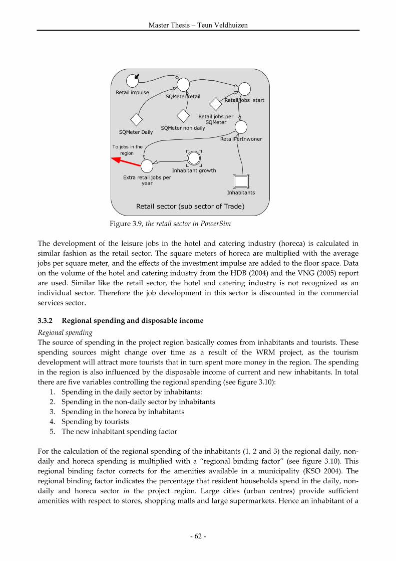
Master Thesis – Teun Veldhuizen
- 62 -
Figure 3.9, the retail sector in PowerSim
The development of the leisure jobs in the hotel and catering industry (horeca) is calculated in
similar fashion as the retail sector. The square meters of horeca are multiplied with the average
jobs per square meter, and the effects of the investment impulse are added to the floor space. Data
on the volume of the hotel and catering industry from the HDB (2004) and the VNG (2005) report
are used. Similar like the retail sector, the hotel and catering industry is not recognized as an
individual sector. Therefore the job development in this sector is discounted in the commercial
services sector.
3.3.2 Regional spending and disposable income
Regional spending
The source of spending in the project region basically comes from inhabitants and tourists. These
spending sources might change over time as a result of the WRM project, as the tourism
development will attract more tourists that in turn spent more money in the region. The spending
in the region is also influenced by the disposable income of current and new inhabitants. In total
there are five variables controlling the regional spending (see figure 3.10):
1. Spending in the daily sector by inhabitants:
2. Spending in the non-daily sector by inhabitants
3. Spending in the horeca by inhabitants
4. Spending by tourists
5. The new inhabitant spending factor
For the calculation of the regional spending of the inhabitants (1, 2 and 3) the regional daily, non-
daily and horeca spending is multiplied with a “regional binding factor” (see figure 3.10). This
regional binding factor corrects for the amenities available in a municipality (KSO 2004). The
regional binding factor indicates the percentage that resident households spend in the daily, non-
daily and horeca sector in the project region. Large cities (urban centres) provide sufficient
amenities with respect to stores, shopping malls and large supermarkets. Hence an inhabitant of a
Retail sector (sub sector of Trade)
SQMeter retail
SQMeter DailySQMeter non daily
Retail jobs perSQMeter
Retail jobs start
Inhabitants
RetailPerInwoner
Inhabitant growth
Extra retail jobs peryear
Retail impulse
To jobs in the region
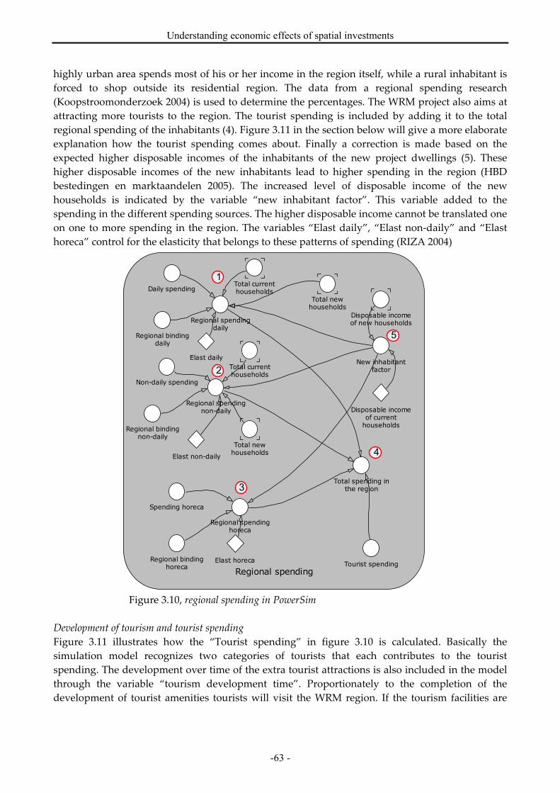
Understanding economic effects of spatial investments
-63 -
highly urban area spends most of his or her income in the region itself, while a rural inhabitant is
forced to shop outside its residential region. The data from a regional spending research
(Koopstroomonderzoek 2004) is used to determine the percentages. The WRM project also aims at
attracting more tourists to the region. The tourist spending is included by adding it to the total
regional spending of the inhabitants (4). Figure 3.11 in the section below will give a more elaborate
explanation how the tourist spending comes about. Finally a correction is made based on the
expected higher disposable incomes of the inhabitants of the new project dwellings (5). These
higher disposable incomes of the new inhabitants lead to higher spending in the region (HBD
bestedingen en marktaandelen 2005). The increased level of disposable income of the new
households is indicated by the variable “new inhabitant factor”. This variable added to the
spending in the different spending sources. The higher disposable income cannot be translated one
on one to more spending in the region. The variables “Elast daily”, “Elast non-daily” and “Elast
horeca” control for the elasticity that belongs to these patterns of spending (RIZA 2004)
Figure 3.10, regional spending in PowerSim
Development of tourism and tourist spending
Figure 3.11 illustrates how the “Tourist spending” in figure 3.10 is calculated. Basically the
simulation model recognizes two categories of tourists that each contributes to the tourist
spending. The development over time of the extra tourist attractions is also included in the model
through the variable “tourism development time”. Proportionately to the completion of the
development of tourist amenities tourists will visit the WRM region. If the tourism facilities are
Regional spending
Disposable incomeof current
households
Disposable incomeof new households
Elast daily
Elast non-daily
Elast horeca
Regional bindingdaily
Regional bindinghoreca
Regional bindingnon-daily
Daily spending
Non-daily spending
Spending horeca
Total spending inthe region
Tourist spending
Regional spendingdaily
Regional spendingnon-daily
Regional spendinghoreca
New inhabitantfactorTotal current
households
Total currenthouseholds
Total newhouseholds
Total newhouseholds
1
5
4
3
2

Master Thesis – Teun Veldhuizen
- 64 -
only 50% finished only 50% of the tourist potential will come to the region. The two tourist types
are:
1. The “day tourists” who visit the region for only one day (data from CVO 2004). The number of
day tourists depends on the amenities in the region. This can be the quality of the nature,
swimming water, sailing docks, a beauty centre, hotels and restaurants or a museum. The CVO
measures the spending patterns of tourists and based on this information a daily sum of money
can be attributed to each tourist. Hence multiplying the daily spending and the amount of
tourists gives “total spending of day tourists”.
2. The holiday tourists who visit the region for multiple day’s using accommodation in the
region. Just as the day tourists what holiday tourists spend on average is multiplied with the
total number of holiday tourists. The amount of tourists in the region also depends on the
“ambition level” and the progress of the project. The ambition level gives the model user
control over the flow of tourists into the region. Standard the ambition level is set to receive
half a percentage of the total tourism in the three adjacent tourist regions Waddenzee,
IJsselmeer and Noordzee badplaatsen (Alterra 2005).
Figure 3.11, tourism spending in PowerSim
Calculation of disposable income of new inhabitants
On order to get an estimate for the disposable income of the new inhabitants the average price of
the new dwellings in the project region is coupled to the disposable income (see figure 3.12). By
calculating the costs of owning a house (“average
housing costs”) from the “average project house
costs” and the “interest” level a measure is given for
the disposable income. The average housing cost is
finally divided through the average percentage
people spend on their house compared to their
disposable income, the “Habitat quote” (Woonquote,
CBS).
Figure 3.12, disposable income of new inhabitants
Disposable income of the newinhabitants
Interest
Average projecthouse cost
Average Housingcosts
Disposable incomenew inhabitants
HabitatQuote
Tourism spending
Total spending daytourists
Total spending ofholiday tourists
Total tourismspending
Number of daytourists
Spening daytourism Spending holiday
tourism
Number of holidaytoursist
Ambition level ofproject
Total Dutch holidays
Tourismdevelopments
Tourismdevelopment time Building delay
To spending in the regon
12

Understanding economic effects of spatial investments
-65 -
3.3.3 Inhabitant and available labour force developments
Development of inhabitants and labour force
The development of inhabitants in the simulation model is depicted in figure 3.13. Through the
“Inhabitant rate” (1) the predicted population development by the PRIMOS model (Heida 2002)
serves as input for the “inhabitants growth rate”. The variable “new inhabitants” indicates the new
residents in the region that are caused by the Wieringerrandmeer project. The stock of inhabitants
(“inhabitants in the region”) represents all the residents in the project area. The inhabitants are
divided into four age groups (0-15, 15-30, 30-65, 65+). The PRIMOS model provides an age
distribution that follows these four age groups. The “new inhabitants” automatically receive the
age distribution that is present in the region at time of entrance. However it is also possible to
manually adjust the age distribution with the “new inhabitants age distribution” variable. This
gives the model user the opportunity to see the effects on the region if for instance only senior
inhabitants are attracted to the WRM. The age groups are also used to deduct the “potential labour
force” for the calculation of the labour force in the region (3). The latter variable is used to select
only the age groups 15-30 and 30-65, which in the shift-share analysis functions as indicator of the
supply of labour in the region (see figure 3.6). More information on how PowerSim copes with age
and household distribution can be found in appendix 8
Figure 3.13, inhabitants and labour force in PowerSim
Just as the age distribution does the composition of the households also consists of four categories
(single, single parent, living together no kids, living together with kids). And in similar fashion
when nothing is done the model increases the households with the same distribution as currently
present in the model. This method is also used for the development of the households in the
region.
Inhabitants and labour force
#
Potentail labourforce
Labour force
Working labourforce
Gross participation
Inhabitants in theregion
Inhabitants growthrate
Inhabitant rate
Total inhabitants
Age distribution
New inhabitants
Unemployment
New inhabitantsage distribution
2
1
3
To shift share analysis

Master Thesis – Teun Veldhuizen
- 66 -
3.4 Assumptions made during the development of the simulation
model
During the development of the concept model and the translation to the actual simulation model,
several assumptions have been made in order to come to the instrument presented in section 3.3.
Sections 3.4.1 to 3.4.3 describe for each model component what the most important assumptions
are. The model components are divided in similar fashion as section 3.3 and elaborate on
statements made in that section:
3.4.1 Labour markets in the basic and non-basic sectors
3.4.2 Regional spending and disposable income
3.4.3 Inhabitants, available labour force and housing developments
Each assumption that is discussed is also analyzed on its effects on the model outcomes with
respect to sensitivity. A more elaborate sensitivity analysis is referred to in chapter 4 where the
model is validated.
3.4.1 Assumptions: labour markets in the basic and non-basic industry sectors
Jobs-follow-people
Theoretical evidence can be found both for the hypothesis that people-follow-jobs as for jobs-
follow-people (see section 2.3.3). In the thesis model the latter hypothesis is chosen for two
reasons. First, empirical evidence can be found for jobs-follow-people and not for people-follow-
jobs. Vermeulen, Verkade and Van Ommeren (2005, 2006) have shown this empirical proof in a
series of publications based on historical data. Second in a recent publication Derks et al. (2006)
mention that the Dutch population growth is gradually grinding to a halt. Already in the next
decennium, less people will be available on the labour market. Derks predicts that from 2035 the
Dutch population will shrink. This development makes labour an even more important and scarce
production good and if firms want to maintain in business they have to settle where labour is still
available. This means that if relatively a lot of people (potential labour force) live in an area
compared to work a region, that region becomes more attractive for employers to locate. This leads
to an – higher than – average increase in jobs. This effect is included in the shift-share analysis that
is used for the calculation of jobs in the project region.
Decreasing importance of the historic over-performance in the shift-share analysis
The previous assumption that job-follow-people is incorporated in the model through the shift
factor. This is similar to the way that Koops & Muskens (2005) describe the inclusion of different
variables in the shift in the REGINA model. The shift-factor of the shift-share analysis depends
both on the historic performance as on the jobs-follow-people theory. The historic performance
however diminishes over the years while at the same time the availability of labour factor
increases (see figure 3.14). The slope in the model is currently set to reach 0% historic performance
value in 15 years according to a linear function. The model includes the possibility to change the
linear function into an exponential and logarithmic function. It is also possible to adjust the 15
years historic performance influence. This assumption is not overly sensitive to changes in the
decay time of 15 year.

Understanding economic effects of spatial investments
-67 -
Figure 3.14, adaptive shift factor for determining job development
The maximum and minimum values of the available labour component of the shift factor
The regional performance factor in the shift-share analysis of available labour is calculated by
comparing the national with the regional average available labour. The number that is obtained
from this equation is dimensionless and has to be linked to a growth indicator (see also figure 3.6).
To prevent one-time historic events from influencing the extrapolation of data to extreme values,
the maximum value of the available labour component has been set on 1 time the standard
deviation32 of the national job development (Nijkamp & Reggiani 1998). This prevents extreme,
and irresponsible, growth in jobs in the region. The same is done for the minimum value. This
assumption does not show irresponsive outcome bounds.
Lack of sector specification in working labour force in region
Ideally the “Working labour force in the region” is modelled the exact same way as the “Jobs of
employees in the region”, however due to a lack of data this is not possible (CBS data not
available). The data available for “Jobs of employees in the region” stems from the CPB scenarios
and is used to calculate the gross region product through shift-share analysis (Huizinga & Smid
2004). The “Working labour force in the region” on the other hand is derived from the PRIMOS
and does not include information that is specified on an industry sector level. Therefore the
“Working labour force in the region” is given only in total sector working labour force output.
Older population requires more healthcare
Because the autonomous scenario of the Wieringerrandmeer shows a higher increase of “old”
inhabitants compared to the Netherlands the jobs in healthcare in the region will rise faster. In
order to correct this error a variable is included that attributes twice the amount of healthcare jobs
when the population ages more than the national average. This is in accordance with a market
study of the healthcare industry executed by the ministry of Health (Branche rapport zorg sector
2005). Sensitivity analysis showed that the amount of twice as much healthcare for population over
65 is not overly sensitive.
3.4.2 Assumptions: regional spending and disposable income
Production sector reduction
The Dutch production sectors are divided into 15 major groups, this is visible on the left side of
figure 3.15. These 18 sectors are not all included in the simulation model for two reasons. First,
including 18 sectors will make the model more complex, decreasing the usability. Second, not all
the data for all the sectors are known. The data from sector C (mineral extraction) and E (e.g.
32 From discussion with Michiel Pellenbarg
time
ShiftDeclining influence of historic
sector growthIncreasing influence
of available labour
time
ShiftDeclining influence of historic
sector growthIncreasing influence
of available labour

Master Thesis – Teun Veldhuizen
- 68 -
energy sector) for instance are often not publicly available and can therefore not be used33. By
subtracting data from other sectors, it is possible to combine sectors C, D and E into one industry
sector. The effect of this assumption on the model is that a less detailed description can be given of
the production sector in matter of financial performance and employment.
Figure 3.15, production sector reduction
Disposable income of inhabitants of the project dwellings
The dwellings in the WRM project are expected to be far more expensive compared to the existing
housing prices in the WRM region. Therefore it can be expected that the inhabitants of these new
dwellings will have a higher disposable income compared to the existing inhabitants. The
assumption that lies at the basis of this theory is that, on average, each household spends 25% of
their disposable income to their housing costs34 (Woonquote, CBS). Using this “habitat quote”, the
house price and the mortgage interest rate the disposable income of new inhabitants can be
calculated (RIZA 2005).
Elasticity in disposable income
A higher disposable income changes the amount of money that people spend in their region. To
calculate the development in the increase of spending in the region the increase of disposable
income has to be corrected for product elasticity. For the daily sector this is 25%, for the non-daily
sector 50% and for leisure 100% (source: RIZA 2004). The elasticity percentages are relatively
sensitive as they directly control the consumption in the region.
Regional binding as factor for determining regional spending
The regional spending can be calculated by multiplying the average income with the households
in the region. However, depending on the properties of the region only a portion of this income is
spent in the residential region. Inhabitants of regions with high amenity levels (mega stores,
shopping centres and large supermarkets) spent more of their disposable income in their
residential region than inhabitants of low amenity regions (KSO 2004). This translates into a factor
controlling the regional (economic) binding of inhabitants to a region. Based on the
33 Because the government is/was shareholder of a lot of the NUTS companies in the Netherlands the data on
these economic activities is classified. 34 Only for home owners, the habitat quote for rental homes is about 30%
A Landbouw, jacht en bosbouwB VisserijC DelfstoffenwinningD IndustrieE Openbare voorzieningsbedrijvenF Bouwnijverheid BouwnijverheidG Reparatie consumentenart; handel HandelI Vervoer, opslag en communicatie Vervoer en communicatieJ Financiële instellingen Financiële instellingenK Verhuur; zakelijke dienstverleningH HorecaL Openbaar bestuur; soc verzekeringM OnderwijsO Cultuur, recreatie; ov dienstverlN Gezondheids- en welzijnszorg Gezondheids- en welzijnszorg
Landbouw
Nijverheid (excl. bouw)
Overige niet-commerciele dienstverlening
Zakelijke dienstverlening

Understanding economic effects of spatial investments
-69 -
Koopstroomonderzoek three region sizes are accounted for: small, middle and large regional city
types (see table 3.1). There are also three different factors for binding: the daily sector (general
daily groceries), the non-daily sector (electric appliances, furniture, etcetera) and Leisure (pubs,
hotels, restaurants, bike rent). The inhabitants of the Wieringerrandmeer spend 85% of their daily
shopping, 40% of their non-daily shopping and 30% of their leisure expenses in the project region.
Table 3.1, the regional spending index
3.4.3 Assumptions: inhabitants, available labour force and housing developments
Households are equal to the amount of dwellings
A house cannot be empty therefore a one on one relationship between the amount of dwellings
and the amount of households. This also means that institutional households are not taken into
account. This leads to an error percentage that is less than 0,1% and is therefore neglected (CBS,
inhabitant data 2005).
Transition from “Potential labour force” to “Labour force”
In order to translate the potential labour force into labour force a variable is needed that indicated
the gross participation. The Social and Cultural Planning Office of the Netherlands (SCP) provides
both current participation degrees as predictions on participation. The former is available on
COROP region level, and the latter only on national level. The national prediction has to be
differentiated to regional values based on the current participation (Sociaal Cultureel Planbureau,
2004). Gross participation is derived from historical data and is assumed in most scenarios to
converge to 63%. Sensitivity analysis did not show that the gross participation is unacceptable
sensitive.
Transition from “Labour force” to “Working labour force”
The factor unemployment expresses the relation between the labour force and the working labour
force. Unemployment differs per region and will generally not be based on the production sectors
due the fact that the potential labour force data is not sector specific. The estimation of the
unemployment stems from the CPB scenarios where in the best scenario the unemployment
reaches to 4% and in the worst case more than 7% (Huizinga & Smid 2004). Sensitivity analysis did
not show that the unemployment factor is unacceptable sensitive.
No building delay during the project
The assumption is made that if the project starts there will be no further delays. This also means
that there are sufficient buyers for the new dwellings and that and that new households move in
directly into the new dwelling. This in turn means that a new dwelling can never be empty
No inclusion of rental homes
The simulation model does not include the possibility of differentiating between an owner
occupied house and a rented house. This assumption based on the Wieringerrandmeer case where
all the new housing projects are commercially sold to homeowners.
Percentage of income spent in regionCity type Inhabitants Daily Non-daily LeisureSmall town (rural) < 15.000 85% 40% 30%
Medium sized citybetween 15.000 and 200.000
90% 70% 65%
Large city > 200.000 95% 80% 85%

Master Thesis – Teun Veldhuizen
- 70 -
3.4.4 Simulation model settings
• Run length: the current plans for the Wieringerrandmeer have an execution time of more than
twenty years. The run length is therefore set on 25 years.
• Start time: the start time of the simulation model is 2005. This means that all the values that are
used in the simulation models are discounted to mach the price level in the year 2005.
• Time step: the time step controls for a large part the speed of a simulation run. When set very
small, one simulation run can take minutes. However when the time step is set too large the
model outcomes are less accurate. Taking into account the user requirements and the fact that
the run length is 25 year a time step of 10 days is taken.
• Calendar: in PowerSim the bank calendar is used. This calendar has 12 months consisting each
of 30 days; hence a year has 360 days.
• Integration settings: the most accurate integration method is used for the calculation of the thesis
model, 4th order, Runge-Kutta (fixed step).
For the sensitivity analysis of the input variables several other settings were used:
• Risk analysis method: the most detailed risk analysis method is used in the simulation model for
sensitivity analysis. The Latin Hypercube method correlates each different simulation run to
the previous runs that are executed. This makes this method more effective that for instance
Monte Carlo simulation and therefore less iteration steps are necessary.
• Run count: the run count is the number of simulation runs that is used to calculate the
predictability intervals. The higher the number of simulation runs the larger the power of the
statement on the predictability bounds of a variable. Unless specified otherwise the standard
run count setting is 40 runs.
• Seed value: the seed value determines the kick-off value of the random number generator.
Fixing the seed value ensures that model results can be repeated. The standard PowerSim
setting is 100 and this value is always used.
3.5 User interface: communicating with policy makers and
consultants
Because a lot of requirements revolve around the presentation of outcomes this section elaborated
on the user interface of the simulation model. The user interface is basically what the model user is
able to see when working with the model. Working with a simulation model is difficult enough
and therefore the model output should be served in ready to eat packages. The requirement
analysis demands in the communication issues that the following problems have to be “solved” by
the user interface (see also section 2.5):
• Avoid large tables, use graphs, limit graphs, information of input and output variables.
• Facilitate novice and advance user options (the “Jip & Janneke” version).
• Display projections of: housing market, employment, regional economy and economic
scenarios.
• Understanding what to do should take no more than 5 minutes.
• Give an indication of the variable bounds.
• Visualize model relations.

Understanding economic effects of spatial investments
-71 -
3.5.1 A standardized layout for simple understanding
To improve the user-friendliness and keep an easily adjustable format for the interface a standard
layout is chosen that can be adjusted for each purpose. In figure 3.16 this standard format is
illustrated. The basic page consists of a header displaying the main fields of interest: housing,
working and the regional economy. The fields of interest are underlined, as that is the regular
format for illustrating hyperlinks. Figure 3.16 specifically shows the housing page and the
inhabitants grouped by age sub-menu. The header is always visible and never leaves the screen,
just like an Internet Explorer does with the address bar. The tablet on the left side shows the
possible options in the housing menu. In this case dwellings, inhabitants and age (depicted in
figure 3.16) and inhabitants and household type. By pressing on the hyperlinks in the tablet a new
page is called that illustrated the requested information. What also is standard is the large graph in
the middle, a tablet on the right for additional options and the advanced menu. The table at the
bottom can illustrate different extra information or remain blank. The autonomous scenario is
always depicted in blue while the WRM GO scenario is always pink. The central graph shows
different variables depending on the chosen sub-menu and so does the table at the bottom. The
options tables let’s people work with the model, make small adjustments in the assumptions or
choose a different economic scenario. The advance option is in this case the possibility to adjust the
composition of the households that move to the region as a result of the investment project. By
clicking on the hyperlink another page is called with the advanced option.
MENU:selecteergewensteinformatie
LEGENDA
Inwoners naar leeftijd
Geen WRM WRM GO!
Grijze druk in de regio 0,23 0,22
Grijze druk nationaal 0,22 0,22
Totaal aantal inwoners in projectgebied 21.616 Inwoner 25.822 Inwoner
Non-commercial use only!
Opties
Geen WRM
WRMproject GO!
Aanvullende informatie
1 jan 2005 1 jan 2010 1 jan 2015 1 jan 2020 1 jan 2025 1 jan 2030
3.000
6.000
9.000
Inwoner
Non-commercial use only!
Leeftijdgroepen
NulVijftien
VijftienDertig
DertigVijfenzestig
VijfenzestigPlus
Advanced
Leeftijdopbouw
Gelijk aan huidig
Handmatig instellen
HOME Wonen Werken Economie ? & HELP
Leeftijds-opbouw
Woningen inde regio
Huishoud-type
Leeftijdsopbouw vannieuwe inwoners
aanpassen
Figure 3.16, the standard layout for the model interface (the housing page)

Master Thesis – Teun Veldhuizen
- 72 -
Each sub-menu has its own help file, assisting model users in coping with the model or finding
information about the variables (see figure 3.17). Again the header bar remains similar and with
the sub-menu on the right different subjects can be chosen. The help menu also contains
information concerning the project (about) and the basic principles of system dynamics.
The user interface offers the possibility of novice and advanced users and by only showing 1 graph
approximates a “Jip & Janneke” version. Besides it still remains possible to adjust the entire model
and add components in the PowerSim construction mode. With respect to constructing the
interface, PowerSim is not the most convenient program to work with. Because PowerSim does not
use an object-oriented manner of working, each page that is shown in the interface has to be built
individually. This makes adjusting it more complex and more prone to faults.
MENU:selecteergewensteinformatie
De grafieken
Bouwvertraging geeft de mogelijkheid to het
instellen van een verlating van de ingangzettingvan het project. Met de schijfcontroler kan de
bouw 2000 dagen (5,5 jaar) uitgesteld worden.
Aanvullende informatie
Bouwvertraging
Advanced: Leeftijdopbouw
aanpassen
De grafiek "ontwikkeling van woningen in de regio"
geeft een voorspelling van het aantal huizen dat inde regio gebouwd gaat worden. De x-as geeft de
tijd in jaren weer en de y-as geeft het aantalwoningen weer.
De grafiek "inwoners naar leeftijd" geeft eenvoorspelling per leeftijdsgroep van het aantal
inwoners dat in de regio woont. Door rechts, onder"leeftijdsgroepen" op de verschillende knoppen te
drukken worden verschillende leeftijdsklassen
zichtbaar. De x-as geeft de tijd in jaren weer en dey-as geeft het aantal inwoners weer.
De grafiek "inwoners naar huishoudtype" geeft een
voorspelling van het aantal huishoudens dat in de
regio woont. Door rechts, onder "Huishoudtype"op de verschillende knoppen te drukken worden
verschillende huishoudens zichtbaar.De x-as geeftde tijd in jaren weer en de y-as geeft het aantal
woningen (huishoudens) weer.
Advanced: Huishoudtype aanpassen
Het model biedt de mogelijkheid tot het aanpassen
van de leeftijdopbouw van de nieuwe inwoners van
het project gebied. Standaard is ingesteld dat deleeftijdsopbouw van nieuwe inwoners gelijk is aan
de huidige opbouw. Door de knop "handmatiginstellen" aan te zetten is vervolgens via de
onderstaande hyperlink de opbouw handmatig te
regelen. Volg verdere instructies aldaar.
Het model biedt de mogelijkheid tot het aanpassen
van het huishoudtype van de nieuwe inwoners van
het project gebied. Standaard is ingesteld dat dehuishoudtype- verdeling van nieuwe inwoners gelijk
is aan de huidige verdeling. Door de knop"handmatig instellen" aan te zetten is vervolgens
via de onderstaande hyperlink de verdeling
handmatig te regelen. Volg verdere instructiesaldaar.
HOME Modelhulp About System Dynamics ? & HELP
Wonen HELP
Werken HELP
EconomieHELP
Begrippen
Bruto regionaalproduct
Figure 3.17, the standard layout for the model help interface (housing help page)

Understanding economic effects of spatial investments
-73 -
3.6 Conclusions of the model construction
In chapter 3 the second thesis sub question formed the departure point for the construction of the
thesis instrument. Two translations had to be made to come to the final simulation model. The
translation of the requirement-, literature and other regional economic model studies in a concept
model first and then the translation of this concept model into the final simulation model.
How to construct an instrument for the ex-ante exploration and assessment of policy options in spatial
investments in a region?
a. How are the notions from the requirement analysis, literature study and existing models translated
into a conceptual model?
b. How is this conceptual model translated into a mathematical simulation model?
The requirements found in the literature and in the requirement interviews (see chapter 2) formed
the basis of the concept model. By identifying the important model variables from the requirement
interviews the literature handed the relationships between these variables. Then the existing
models showed some interesting characteristics or insights that provided useful in the second
translation (concept to quantified model). When the conceptual model was finished it had to be
translated into the actual simulation model using PowerSim and Excel. The interaction between
these two software programs is not optimal; the communication between them can be called
clumsy and slow (see appendix 9). Initially the model was intended to incorporate a lot of aspects
and causal relationships from the Urban Dynamics model from Forrester. However when the first
translation started it appeared that the user requirements were hard to match with some of the
properties of the UD model. The geographical scale of the model of Forrester was hard to extract
because it is based on a small town that grows into a metropolis. This growth period was also a
problem because the UD model was made to calculate the developments of a city over a period of
250 years while the thesis project is only interested in a ten times smaller runtime.
During the development of the concept other assumptions had to be made as well. Because it is not
realistic to extrapolate the historic performance in the shift-share analysis indefinite a control
mechanism is built in. The availability of labour gradually replaces the overrepresentation of the
industry sectors (the jobs-follow-people theorem). The translation of the concept model to the
simulation model also required a series of assumptions. In the model it is for instance not possible
for dwellings to be uninhabited. Uninhabited dwellings make up an insignificant part of the total
supply of dwellings. By leaving the empty dwellings out the model became much less complex
because households and dwellings could be coupled to each other. Another assumption that is
made for the sake of simplicity is the reduction of the 15 basic industry sectors to only 9.
The fact that an actual case model had to be developed meant that actual data was going to be
needed for the input of the model. This meant that the basic structures of the UD model could not
be used, as the variables of the UD model did not match the required outcomes. The fact that
actual data had to be used also meant that the UD model could not be validated, as it is a
theoretical model. Furthermore, it became clear that the model components that had to be
developed to display system behaviour (like demographic development) would become very
complex. The complexity was of such extent that the requirement to create a small model had to be
left. In order to solve the latter problem exogenous data was used to replace the model

Master Thesis – Teun Veldhuizen
- 74 -
components that caused the extreme complexity. Other economic models also used this principle
and the required data was available through PRIMOS (Heida 2002). The system dynamics
methodology however appears to have some side effects with respect to the use of exogenous
variables. This causes the model feedback loops to collapse defying the purpose of the system
dynamics model from the beginning. It must be said however that the other concepts of system
dynamics still hold and that providing insight with a system dynamics interface is still possible.
See section 5.1 for a more elaborate explanation.
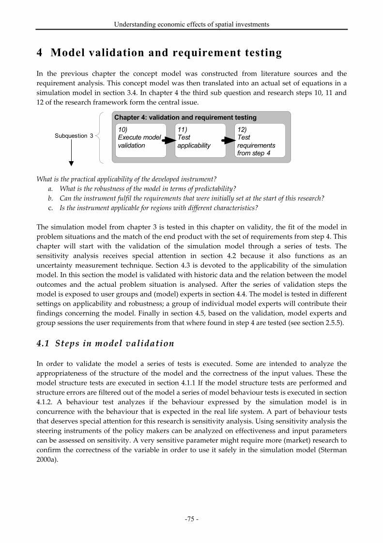
Understanding economic effects of spatial investments
-75 -
4 Model validation and requirement testing
In the previous chapter the concept model was constructed from literature sources and the
requirement analysis. This concept model was then translated into an actual set of equations in a
simulation model in section 3.4. In chapter 4 the third sub question and research steps 10, 11 and
12 of the research framework form the central issue.
What is the practical applicability of the developed instrument?
a. What is the robustness of the model in terms of predictability?
b. Can the instrument fulfil the requirements that were initially set at the start of this research?
c. Is the instrument applicable for regions with different characteristics?
The simulation model from chapter 3 is tested in this chapter on validity, the fit of the model in
problem situations and the match of the end product with the set of requirements from step 4. This
chapter will start with the validation of the simulation model through a series of tests. The
sensitivity analysis receives special attention in section 4.2 because it also functions as an
uncertainty measurement technique. Section 4.3 is devoted to the applicability of the simulation
model. In this section the model is validated with historic data and the relation between the model
outcomes and the actual problem situation is analysed. After the series of validation steps the
model is exposed to user groups and (model) experts in section 4.4. The model is tested in different
settings on applicability and robustness; a group of individual model experts will contribute their
findings concerning the model. Finally in section 4.5, based on the validation, model experts and
group sessions the user requirements from that where found in step 4 are tested (see section 2.5.5).
4.1 Steps in model validation
In order to validate the model a series of tests is executed. Some are intended to analyze the
appropriateness of the structure of the model and the correctness of the input values. These the
model structure tests are executed in section 4.1.1 If the model structure tests are performed and
structure errors are filtered out of the model a series of model behaviour tests is executed in section
4.1.2. A behaviour test analyzes if the behaviour expressed by the simulation model is in
concurrence with the behaviour that is expected in the real life system. A part of behaviour tests
that deserves special attention for this research is sensitivity analysis. Using sensitivity analysis the
steering instruments of the policy makers can be analyzed on effectiveness and input parameters
can be assessed on sensitivity. A very sensitive parameter might require more (market) research to
confirm the correctness of the variable in order to use it safely in the simulation model (Sterman
2000a).
Chapter 4: validation and requirement testing
10) Execute model
validation
12)Test
requirements from step 4
Subquestion 311)Test
applicability

Master Thesis – Teun Veldhuizen
- 76 -
4.1.1 Model structure tests
Model structure tests assess the simulation model on structural errors that could have creped in
during model construction. If any errors are detected they are dealt with immediately, unsolvable
errors are reported in the text and should be considered when using the model. In total 6 structure
tests are performed. The first three focus on the translation of the concept model into the
simulation model and the correctness of data that is used as input parameter. Test 4 to 6 tests if the
model responds to abrupt changes in the system as it is supposed to react. Test 6 is specially
intended to see if the chosen integration method and step is appropriate for this model (Sterman
2000a).
1) Parameter assessment is a method for checking both the real life meaning of the input variables
and the correctness of these variables. In the assessment of available data in the thesis project
in section 2.6 different information sources have been identified. Most of the input values
have been either deducted with statistical methods or estimated from literature or other
available model. Most of the input data has already been described in the assumptions of the
simulation model in section 3.4. The following list gives an overview of the input parameters
that might require more attention and that will have to be tested in the sensitivity analysis
a. The regional binding factors that have been deducted from the
“Koopstroomonderzoek” (KSO 2004) are not available for the WRM region. Therefore
special attention should be paid when using these input parameters.
b. The elasticity of the income of the new inhabitants of the project region has been
collected from the RIZA (2004). However more complex elasticity equations and
perhaps also estimation are available.
c. The input data for the autonomous development of the inhabitants, dwellings and
households in the project region comes from the PRIMOS database (Heida 2002). If
newer versions of PRIMOS would make better estimations of these parameters, these
new values should be used.
d. Special attention should be given to the parameters in the calculation of the tourist
spending. The estimation of day tourists is based on the Socio-economic Effect Study
(DHV 2005) while more accurate data might be available from sampling in the project
region.
2) Structure assessment is a method for checking whether the model corresponds to the
knowledge of the real world system and if. The level of aggregation between the sub models
of the simulation model is a little bit skewed. This means that some parts of the model are
worked out in more detail compared to the rest of the model. This is mainly caused by two
items in the simulation model:
• One of the user requirements was to analyze the tourism effect on the regional economy.
In order to do this an extra model component was added (see figure 3.11) that provided
the necessary data.
• Because the jobs in the non-basic sectors could not be calculated with the shift-share
analysis separate model components were constructed to deal with the job development
in these sectors (see figure 3.8 and 3.9). These components also have a higher level of
detail compared to the job development in the basic industry sectors.
When dealing with a skewed model it is important not to let the highly detailed model
sections take up an unjust large part of the model outcomes (Sterman 2000a).

Understanding economic effects of spatial investments
-77 -
3) Dimensional consistency assesses if there are errors in the chosen dimensions in the simulation
model. There is 1 dimensional inconsistency that might cause some confusion with the
model users. In the user interface the distribution of households is not indicated in
households but in dwellings35. This error can occur because household is not included as a
model dimension in the simulation model.
4) Boundary adequacy tests if the policy recommendations resulting from the model changes
when the model boundary is extended or if exogenous variables are relaxed. If the boundary
of the model were extended by for instance adding a demographic module, new feedback
loops would arise in the model. This is a known problem that is carefully weighted against
other options and does not compromise the boundary adequacy. If the boundaries of the
exogenous variables are relaxed, the policy recommendations do not change except for two
variables.
• The CPB scenario’s that are use to calculate growth are very sensitive to changes,
especially changes between scenarios can have huge effect on the model outcome.
• The regional binding factors are also very sensitive to changes of their boundary and will
change the model outcomes significantly.
This problem is noted and might be resolved by dimming down the effect of the CPB
scenarios. More information on these variables is given in the sensitivity analysis in section
4.2.
5) An Extreme conditions test is executed to make sure the model presents estimated behaviour
even under extreme conditions. This involves setting variables to infinite, zero or π. Some
errors occurred during these tests that should be regarded when using the simulation model:
• The initial values in the simulation model are unrelated. Therefore if for instance the
initial value of dwellings in the region is set to 0, this does not mean that there are not
inhabitants. This makes it even more important to have all the initial value data set on the
price level of 2005.
• Some constant variables in the model are implemented to assists the user interface, for
instance the variable that controls what economic scenario is used. Due to the use of “If”
statements the model will give erratic data if other values are used in those constants.
6) Integration error tests if the model is sensitive to changes in the time step of the numerical
integration method. The time step is normally set to 10 days. The model outcome of regional
spending differs 0,06% if a 20 days time step is chosen. Using a 1 day time step increases the
accurateness, however it also decreases the simulation speed with a factor 6 taking 30
seconds per simulation run of 25 years36.
4.1.2 Model behaviour tests
Now the structure of the simulation model has been tested it is time to test the behaviour of the
model. The behaviour tests focus more on the conduct of the model during model during changes
in variables and relationships. Two tests will be performed. The behaviour reproduction test
analyzes if the model can constantly reproduce trustworthy data. In the behaviour anomaly test
some assumptions are relaxed to analyze the effect on the model outcomes.
• Behaviour reproduction should be able in every simulation model and is possible through the use
of PowerSim. Because no stochastic variables have been used in regular simulation settings,
35 Mentioned in the consultancy test (section 4.3.2) 36 With computer specs: Pentium4 1,80 GHz processor with 256 Mb RAM and Windows 2000 OS.

Master Thesis – Teun Veldhuizen
- 78 -
this is not a problem. If random behaviour is induced on model variables, it remains possible to
reproduce the exact behaviour due to the adjustability of the random number generator. For
the stochastic values in the sensitivity analysis, the seed value is always set on PowerSim
default (100). The behaviour of the model is fully reproducible. The behaviour reproduction
also entails the reproduction of observed behaviour in the real world system. This is the case
for the used relationships in the model, which translates into the correct behaviour of the
simulation model.
• When testing behaviour anomaly some model assumptions are deleted in order to see what the
reaction of the model is. Some issues arise:
o Because it is possible that the inhabitants do not move into their house directly the time
between moving into the region is delayed with a year (Pipeline delay). This delays the
growth of inhabitants and household also with exactly one year.
o If the assumption is relaxed that the historic performance decreases over time and that
the influence of available labour increases the job development shows a reaction. Because
the historic performance has a higher growth rate compared to the labour availability it
shows a further increase of the jobs in the region.
o In that line of thought if the effect of the available labour force is stronger the opposite
effect mentioned above should take place. When the “Max effect” is increased 4 fold the
effect on the jobs is much higher than that of the historic performance.
o The elasticity has an effect on the regional spending. When the elasticity is set to 0 the
new inhabitants will spend the same amount of money in the region. When all elasticity’s
are set on 100%, their regional spending on daily, non-daily and tourism will increase
with the same amount as their disposable income.
o When the regional binding is omitted from the simulation model regional spending is € 0
per year.
4.2 Sensitivity analysis
Sensitivity analysis is a method for testing the robustness of the simulation model. It checks if the
conclusions drawn from the model outcomes change substantially if the assumptions are relaxed a
small amount. This information is also important for policy makers; it can for instance tell them
what the most “potent” steering variable is. This is the variable that causes the largest effect with
the smallest change. Sensitivity analysis should therefore play a part in the both in model testing
as in the communication towards the policy maker. Not all variables have to be tested on
uncertainty. The input variables tested here are either based on an assumption from section 3.4 or
on a quote in the parameter test in the previous section (Sterman 2000a). To include a measure for
sensitivity a standardized factor is used for each sensitivity calculation, this factor is called
absolute uncertainty (δ). This measure is the bandwidth of the 90% interval, divided by the
average outcome times a 100%. If this figure is small, the variable that is tested is relatively
insensitive; if however the figure is high the variable is very sensitivity to changes in the model
assumptions37. Most of the variables have an uncertainty smaller than 10%, if a variable exceeds
this value it should be labelled as highly uncertain and special attention should be taken in account
when working with this variable. If a variable is found to be very sensitive two issues should be
pointed out. First it should be analyzed if the parameter is accurately determined, and how the
37 From discussion with Bert Schilder, in Risk Analysis this is the common form of indicating risk involved
with a model variable.
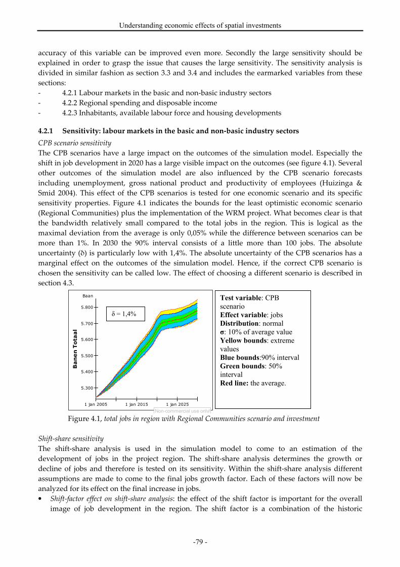
Understanding economic effects of spatial investments
-79 -
accuracy of this variable can be improved even more. Secondly the large sensitivity should be
explained in order to grasp the issue that causes the large sensitivity. The sensitivity analysis is
divided in similar fashion as section 3.3 and 3.4 and includes the earmarked variables from these
sections:
- 4.2.1 Labour markets in the basic and non-basic industry sectors
- 4.2.2 Regional spending and disposable income
- 4.2.3 Inhabitants, available labour force and housing developments
4.2.1 Sensitivity: labour markets in the basic and non-basic industry sectors
CPB scenario sensitivity
The CPB scenarios have a large impact on the outcomes of the simulation model. Especially the
shift in job development in 2020 has a large visible impact on the outcomes (see figure 4.1). Several
other outcomes of the simulation model are also influenced by the CPB scenario forecasts
including unemployment, gross national product and productivity of employees (Huizinga &
Smid 2004). This effect of the CPB scenarios is tested for one economic scenario and its specific
sensitivity properties. Figure 4.1 indicates the bounds for the least optimistic economic scenario
(Regional Communities) plus the implementation of the WRM project. What becomes clear is that
the bandwidth relatively small compared to the total jobs in the region. This is logical as the
maximal deviation from the average is only 0,05% while the difference between scenarios can be
more than 1%. In 2030 the 90% interval consists of a little more than 100 jobs. The absolute
uncertainty (δ) is particularly low with 1,4%. The absolute uncertainty of the CPB scenarios has a
marginal effect on the outcomes of the simulation model. Hence, if the correct CPB scenario is
chosen the sensitivity can be called low. The effect of choosing a different scenario is described in
section 4.3.
Figure 4.1, total jobs in region with Regional Communities scenario and investment
Shift-share sensitivity
The shift-share analysis is used in the simulation model to come to an estimation of the
development of jobs in the project region. The shift-share analysis determines the growth or
decline of jobs and therefore is tested on its sensitivity. Within the shift-share analysis different
assumptions are made to come to the final jobs growth factor. Each of these factors will now be
analyzed for its effect on the final increase in jobs.
• Shift-factor effect on shift-share analysis: the effect of the shift factor is important for the overall
image of job development in the region. The shift factor is a combination of the historic
Test variable: CPB
scenario
Effect variable: jobs
Distribution: normal
σ: 10% of average value
Yellow bounds: extreme
values
Blue bounds:90% interval
Green bounds: 50%
interval
Red line: the average.
1 jan 2005 1 jan 2015 1 jan 2025
5.300
5.400
5.500
5.600
5.700
5.800
Baan
Banen Totaal
Non-commercial use only!
δ = 1,4%
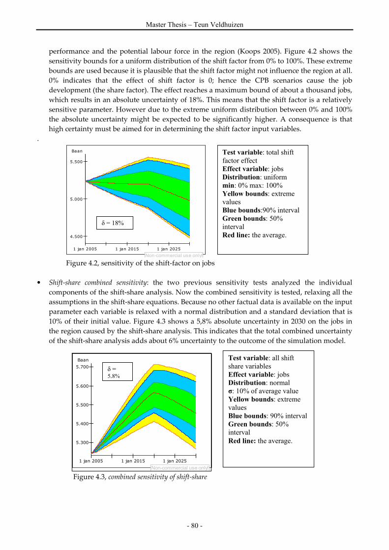
Master Thesis – Teun Veldhuizen
- 80 -
performance and the potential labour force in the region (Koops 2005). Figure 4.2 shows the
sensitivity bounds for a uniform distribution of the shift factor from 0% to 100%. These extreme
bounds are used because it is plausible that the shift factor might not influence the region at all.
0% indicates that the effect of shift factor is 0; hence the CPB scenarios cause the job
development (the share factor). The effect reaches a maximum bound of about a thousand jobs,
which results in an absolute uncertainty of 18%. This means that the shift factor is a relatively
sensitive parameter. However due to the extreme uniform distribution between 0% and 100%
the absolute uncertainty might be expected to be significantly higher. A consequence is that
high certainty must be aimed for in determining the shift factor input variables.
.
Figure 4.2, sensitivity of the shift-factor on jobs
• Shift-share combined sensitivity: the two previous sensitivity tests analyzed the individual
components of the shift-share analysis. Now the combined sensitivity is tested, relaxing all the
assumptions in the shift-share equations. Because no other factual data is available on the input
parameter each variable is relaxed with a normal distribution and a standard deviation that is
10% of their initial value. Figure 4.3 shows a 5,8% absolute uncertainty in 2030 on the jobs in
the region caused by the shift-share analysis. This indicates that the total combined uncertainty
of the shift-share analysis adds about 6% uncertainty to the outcome of the simulation model.
Figure 4.3, combined sensitivity of shift-share
1 jan 2005 1 jan 2015 1 jan 2025
5.300
5.400
5.500
5.600
5.700
Baan
Non-commercial use only!
Test variable: all shift
share variables
Effect variable: jobs
Distribution: normal
σ: 10% of average value
Yellow bounds: extreme
values
Blue bounds: 90% interval
Green bounds: 50%
interval
Red line: the average.
δ = 5,8%
1 jan 2005 1 jan 2015 1 jan 2025
4.500
5.000
5.500
Baan
Non-commercial use only!
Test variable: total shift
factor effect
Effect variable: jobs
Distribution: uniform
min: 0% max: 100%
Yellow bounds: extreme
values
Blue bounds:90% interval
Green bounds: 50%
interval
Red line: the average.
δ = 18%

Understanding economic effects of spatial investments
-81 -
4.2.2 Sensitivity: regional spending and disposable income
Regional binding factor sensitivity
The regional binding corrects for the amount of disposable income that inhabitants of the project
region spend inside the project region. For a rural area this amount is lower compared to a high
amenity urban area (KSO 2004). Figure 4.4 shows the uncertainty bounds when the regional
binding factors for daily, non-daily and recreation are relaxed. The binding factors are quite
sensitive; the absolute uncertainty is 21% in 2030, indicating that this variable plays an important
role in determining regional spending.
Figure 4.4, effect of regional binding on regional spending
Because of the importance in determining the regional spending the values of the regional binding
variables should perhaps be research deeper. Executing a market research that assesses for the
WRM region what the regional binding is compared to daily, non-daily and leisure spending can
for instance do this. Another option would be to initiate a regional binding research for the
province of North Holland just like the “Koopstroomonderzoek” for central Holland. Furthermore
the sensitivity of this variable should be kept in mind while processing the outcomes related to
regional spending.
New dwelling price sensitivity
The disposable income of the new inhabitants is based on the value of the houses that will be built
in the region (CBS, woonquote). The sensitivity of the housing price, hence the disposable income
of new inhabitants is tested by relaxing the housing price and testing the effects on regional
spending. From figure 4.5 it becomes clear that the effects increase over time, this is due to the facts
that the inhabitants join the region in-line with the completion of new dwellings. The total
maximal bound in 2030 is about 7 million euro which results in an absolute uncertainty of 2,7% of
the total regional spending. Overall this means that the housing price of the new dwelling is
relatively insensitive. In the end of 2006 more certainty will be given on the average housing prices
as more details of the project are worked out.
Test variable: all regional
binding variables
Effect variable: regional
spending
Distribution: normal
σ: 10% of average value
Yellow bounds: extreme
values
Blue bounds: 90% interval
Green bounds: 50%
interval
Red line: the average.
δ =21,0%
1 jan 2005 1 jan 2015 1 jan 2025
50.000.000
60.000.000
70.000.000
80.000.000
€
regionale bestedingen
Non-commercial use only!

Master Thesis – Teun Veldhuizen
- 82 -
Figure 4.5, effect of housing price on regional spending
Elasticity of disposable income sensitivity
The new inhabitants have different disposable incomes than the current inhabitants. To calculate
how much those new inhabitants contribute to regional spending a set of elasticity rules in
included in the model. The new inhabitants do not spend all the “extra” disposable income in the
region. These elasticity rules are tested on sensitivity in figure 4.6. With a very small absolute
uncertainty of 0,7% the elasticity variables are not very sensitive.
Figure 4.6, effect of price elasticity on regional spending
4.2.3 Sensitivity: inhabitants, available labour force and housing development
The availability of labour bounds sensitivity
To examine the effect of available labour on the jobs in the region more closely the variable
available labour is relaxed. Dividing jobs in the region with the potential labour force in the region
and comparing that to the national average determines the relative supply of labour in the region.
This value is used in the simulation model. Because the effect of the availability of labour increases
over time, the uncertainty bounds do so too (see figure 4.7). The variable is not overly sensitive as
the bounds in 2030 are within a 100 jobs and the absolute uncertainty is 2,8%.
Test variable: house price
Effect variable: regional
spending
Distribution: normal
σ: 10% of average value
Yellow bounds: extreme
values
Blue bounds: 90% interval
Green bounds: 50%
interval
Red line: the average.
1 jan 2005 1 jan 2015 1 jan 2025
65.000.000
70.000.000
75.000.000
€
regionale bestedingen
Non-commercial use only!
δ = 2,7%
Test variable: all elasticity
variables
Effect variable: regional
spending
Distribution: normal
σ: 10% of average value
Yellow bounds: extreme
values
Blue bounds: 90% interval
Green bounds: 50%
interval
Red line: the average.
1 jan 2005 1 jan 2015 1 jan 2025
65.000.000
70.000.000
75.000.000
€
regionale bestedingen
Non-commercial use only!
δ = 0,7%

Understanding economic effects of spatial investments
-83 -
Figure 4.7, availability of labour bounds
Next to the sensitivity of the individual input variables the sensitivity of all the variables together
is analyzed. The effect on the jobs in the region can be seen in figure 4.8 and the effect on regional
spending in figure 4.9. An issue that occurs when all the variables are relaxed without underlying
dependency is that a cancelling out effect reduces the absolute uncertainty38. Therefore it is called
the lower bound of the absolute uncertainty of the entire model. The higher bound can be tested if
all the input variables are made dependent from each other. For instance that an increase of the
regional binding factor in daily shopping will strongly be correlated to the increase of square
meters of retail (KSO 2004). This effect is visible in figure 4.9 where the absolute uncertainty is 1%
lower compared to the individual uncertainty of regional binding factors. The lower bound of the
absolute uncertainty for the jobs in the region is almost 8%, which is higher than measured in other
tests. What this illustrates is that more accurate statements can be made with this instrument on
the development of jobs than on the development of spending in the region. Executing the higher
uncertainty bound is not possible in the PowerSim software as it is not possible to connect two
input variables in the sensitivity analysis.
Figure 4.8, effect of all variables on jobs in the region
38 From discussion with Bert Schilder
1 jan 2005 1 jan 2015 1 jan 2025
5.000
5.100
5.200
Baan
Non-commercial use only!
Test variable: availability
of labour
Effect variable: jobs
Distribution: normal
σ: 10% of average value
Yellow bounds: extreme
values
Blue bounds: 90% interval
Green bounds: 50%
interval
Red line: the average.
δ = 2,8%
1 jan 2005 1 jan 2015 1 jan 2025
5.400
5.700
6.000
Baan
Banen Totaal
Non-commercial use only!
Test variable: all variables
Effect variable: jobs
Distribution: normal
σ: 10% of average value
Yellow bounds: extreme
values
Blue bounds: 90% interval
Green bounds: 50%
interval
Red line: the average.
δ = 7,8%
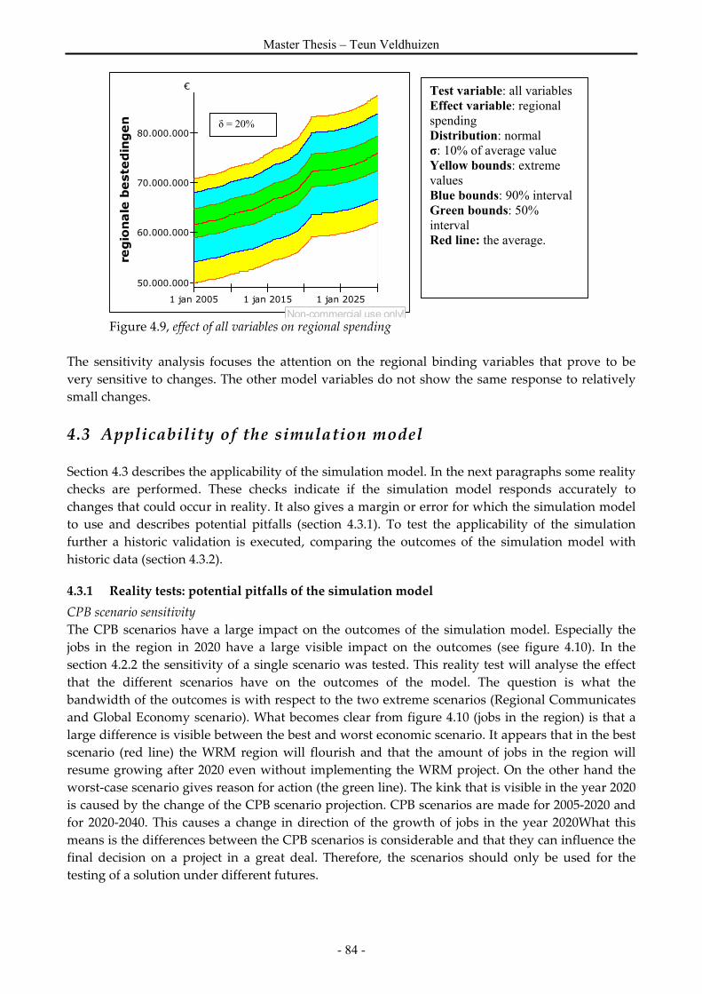
Master Thesis – Teun Veldhuizen
- 84 -
Figure 4.9, effect of all variables on regional spending
The sensitivity analysis focuses the attention on the regional binding variables that prove to be
very sensitive to changes. The other model variables do not show the same response to relatively
small changes.
4.3 Applicability of the simulation model
Section 4.3 describes the applicability of the simulation model. In the next paragraphs some reality
checks are performed. These checks indicate if the simulation model responds accurately to
changes that could occur in reality. It also gives a margin or error for which the simulation model
to use and describes potential pitfalls (section 4.3.1). To test the applicability of the simulation
further a historic validation is executed, comparing the outcomes of the simulation model with
historic data (section 4.3.2).
4.3.1 Reality tests: potential pitfalls of the simulation model
CPB scenario sensitivity
The CPB scenarios have a large impact on the outcomes of the simulation model. Especially the
jobs in the region in 2020 have a large visible impact on the outcomes (see figure 4.10). In the
section 4.2.2 the sensitivity of a single scenario was tested. This reality test will analyse the effect
that the different scenarios have on the outcomes of the model. The question is what the
bandwidth of the outcomes is with respect to the two extreme scenarios (Regional Communicates
and Global Economy scenario). What becomes clear from figure 4.10 (jobs in the region) is that a
large difference is visible between the best and worst economic scenario. It appears that in the best
scenario (red line) the WRM region will flourish and that the amount of jobs in the region will
resume growing after 2020 even without implementing the WRM project. On the other hand the
worst-case scenario gives reason for action (the green line). The kink that is visible in the year 2020
is caused by the change of the CPB scenario projection. CPB scenarios are made for 2005-2020 and
for 2020-2040. This causes a change in direction of the growth of jobs in the year 2020What this
means is the differences between the CPB scenarios is considerable and that they can influence the
final decision on a project in a great deal. Therefore, the scenarios should only be used for the
testing of a solution under different futures.
δ = 7,8%
1 jan 2005 1 jan 2015 1 jan 2025
50.000.000
60.000.000
70.000.000
80.000.000
€
regionale bestedingen
Non-commercial use only!
Test variable: all variables
Effect variable: regional
spending
Distribution: normal
σ: 10% of average value
Yellow bounds: extreme
values
Blue bounds: 90% interval
Green bounds: 50%
interval
Red line: the average.
δ = 20%
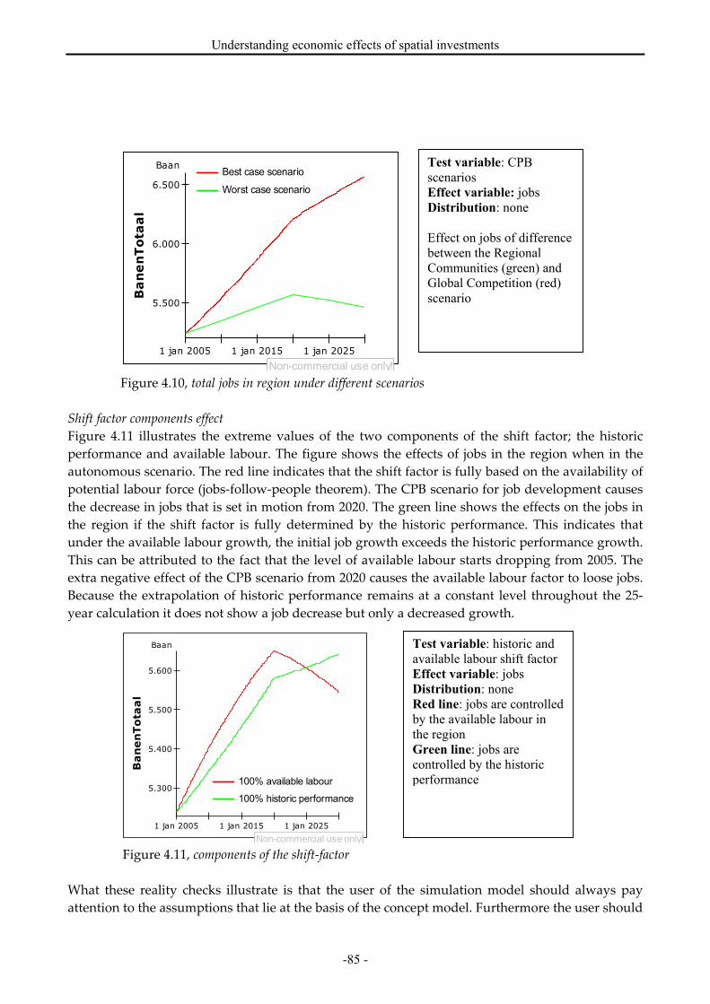
Understanding economic effects of spatial investments
-85 -
Figure 4.10, total jobs in region under different scenarios
Shift factor components effect
Figure 4.11 illustrates the extreme values of the two components of the shift factor; the historic
performance and available labour. The figure shows the effects of jobs in the region when in the
autonomous scenario. The red line indicates that the shift factor is fully based on the availability of
potential labour force (jobs-follow-people theorem). The CPB scenario for job development causes
the decrease in jobs that is set in motion from 2020. The green line shows the effects on the jobs in
the region if the shift factor is fully determined by the historic performance. This indicates that
under the available labour growth, the initial job growth exceeds the historic performance growth.
This can be attributed to the fact that the level of available labour starts dropping from 2005. The
extra negative effect of the CPB scenario from 2020 causes the available labour factor to loose jobs.
Because the extrapolation of historic performance remains at a constant level throughout the 25-
year calculation it does not show a job decrease but only a decreased growth.
Figure 4.11, components of the shift-factor
What these reality checks illustrate is that the user of the simulation model should always pay
attention to the assumptions that lie at the basis of the concept model. Furthermore the user should
1 jan 2005 1 jan 2015 1 jan 2025
5.500
6.000
6.500
Baan
BanenTotaal
Non-commercial use only!
Best case scenario
Worst case scenario
Test variable: CPB
scenarios
Effect variable: jobs
Distribution: none
Effect on jobs of difference
between the Regional
Communities (green) and
Global Competition (red)
scenario
1 jan 2005 1 jan 2015 1 jan 2025
5.300
5.400
5.500
5.600
Baan
BanenTotaal
Non-commercial use only!
100% available labour
100% historic performance
Test variable: historic and
available labour shift factor
Effect variable: jobs
Distribution: none
Red line: jobs are controlled
by the available labour in
the region
Green line: jobs are
controlled by the historic
performance

Master Thesis – Teun Veldhuizen
- 86 -
be aware of the assumptions made in other models, like the CPB scenario predictions. Laymen
might not recognise the “2020 effect” in the outcomes of the model as belonging to the change of
CPB projection.
4.3.2 Validation with historic data
The former section illustrates the caution and knowledge with which to approach simulation
models. It is never certain to what extend the model is predicting the actual developments and
how far it is from the actual future developments. To create some confidence in the outcomes of
the simulation model and as final validation step historic data is used to test the model. The
historic validation has been executed with the time series data from old PRIMOS files, former CPB
scenario forecasts and historic data from the CBS StatLine database. The earliest PRIMOS data that
was available dates back to a prediction of demographic developments in 1997. Because the
simulation model cannot be run without the PRIMOS data the earliest historic analysis dates to the
earliest PRIMOS model. This restricts the historic validation within the time frame from 01-01-1998
until 31-12-2005. Data from the StatLine website from this time period can be used to verify the
outcomes of the simulation model. If the data predicted by the simulation model relates closely to
the actual events, the simulation model can be regarded as fairly capable of predicting socio-
economic developments.
Because a large part of the input data in the model is directly derived from the PRIMOS database,
the quality of the PRIMOS forecast determines for a large part the quality of the outcomes of the
simulation model. Figure 4.12 illustrates the documented inhabitants by the CBS (blue line) and de
the predicted developments by PRIMOS (pink line). On average the predicted value is only 120
inhabitants from the actual value. It can also be seen that between 2002 and 2006 the CBS and
PRIMOS values are vary closely related. However claims are hard to make with only one historic
analysis of only one region, it appears that the predicted value is very much like the actual value.
What can be concluded is that for the purpose of exploring future developments the prediction of
inhabitant growth is valid and sufficiently accurate.
Figure 4.12, forecasted and actual inhabitants
19800
20000
20200
20400
20600
20800
21000
21200
21400
1998 1999 2000 2001 2002 2003 2004 2005 2006
Year
Inhabitants
Inhabitants CBS Inhabitants PRIMOS
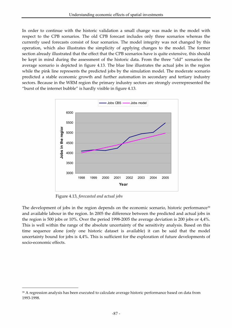
Understanding economic effects of spatial investments
-87 -
In order to continue with the historic validation a small change was made in the model with
respect to the CPB scenarios. The old CPB forecast includes only three scenarios whereas the
currently used forecasts consist of four scenarios. The model integrity was not changed by this
operation, which also illustrates the simplicity of applying changes to the model. The former
section already illustrated that the effect that the CPB scenarios have is quite extensive, this should
be kept in mind during the assessment of the historic data. From the three “old” scenarios the
average scenario is depicted in figure 4.13. The blue line illustrates the actual jobs in the region
while the pink line represents the predicted jobs by the simulation model. The moderate scenario
predicted a stable economic growth and further automation in secondary and tertiary industry
sectors. Because in the WRM region the primary industry sectors are strongly overrepresented the
“burst of the internet bubble” is hardly visible in figure 4.13.
Figure 4.13, forecasted and actual jobs
The development of jobs in the region depends on the economic scenario, historic performance39
and available labour in the region. In 2005 the difference between the predicted and actual jobs in
the region is 500 jobs or 10%. Over the period 1998-2005 the average deviation is 200 jobs or 4,4%.
This is well within the range of the absolute uncertainty of the sensitivity analysis. Based on this
time sequence alone (only one historic dataset is available) it can be said that the model
uncertainty bound for jobs is 4,4%. This is sufficient for the exploration of future developments of
socio-economic effects.
39 A regression analysis has been executed to calculate average historic performance based on data from
1993-1998.
3000
3500
4000
4500
5000
5500
6000
1998 1999 2000 2001 2002 2003 2004 2005
Year
Jobs in the region
Jobs CBS Jobs model

Master Thesis – Teun Veldhuizen
- 88 -
4.4 Performing group and expert tests
In order to get a better, unbiased and hands-on validation of the simulation model and test the
requirements from step 4 (see section 2.5) a number of experts will assess the model. The model
will furthermore be tested on applicability in actual group settings where the model will support
policy development. In total six expert judgements are given, from the policy and consulting field
and also from model experts with experience in spatial economic models (section 4.4.2). The
experts will assess the simulation model for its validity. The principles, assumptions and logical
deductions that are used must together form a consistent whole in order for the simulation model
to be validly usable. In order to test the practical use of the simulation model three group tests will
be performed (4.4.1). One will be a peer-group test that will focus on the model purpose, model
construction and user interface. The test panel will exist from student members that are
knowledgeable on the subject of simulation and system dynamics. The second group test will take
place with consultants of DHV, in this test each member of the test team will take on a role from
which to take a critical look at the model. The third and final group test involved another group of
DHV consultants and focused on the specific use of graphs and table in the presentation of the
outcomes of the model. Appendix 10 gives a more detailed description of the expert interviews
and group tests.
4.4.1 Group validation tests
Three group validation sessions have been executed in order to test and improve the simulation
model. The most important comments, critiques and observations are included in this section, a
more detailed description can be found in appendix 10. Based on the results of the group tests the
simulation model is improved between each groups test. First the aim of the group session is
explained, and then a list of the most important improvements is supplied. Finally a list of
improvements is given that not have been implemented in the simulation model yet.
1. The first test case for the simulation model is the peer group test where a group of students
acts as the advocate of the devil. The graduate students will test the model hands-on and
experience how the model would be used in an actual situation. They were asked to look at the
simulation model both from different actor viewpoints especially that of a policy maker and a
consultant.
2. The most important results of the first group test, the peer-group, have been incorporated
before the second group test. During the second test of the simulation model the actor role
principle is explored in more detail. Due to the political sensitivity surrounding the
Wieringerrandmeer project the case cannot be tested with the municipalities of Wieringen and
Wieringermeer. Therefore a group of 6 members of the DHV E&R staff will participate in the
model test acting as important stakeholder in the Wieringerrandmeer case. Before the session,
each participant received a short introduction that described the purpose of the test and the
role they will “play”.
3. The final group test did not focus on actor roles. It focussed on how the information, the model
outcomes, is displayed in the simulation model interface. A group of 4 member of the
Management Consultancy department of DHV participated in this test.

Understanding economic effects of spatial investments
-89 -
Remarks made during the group tests that have been dealt with.
• The information on the outcomes of the simulation model must be displayed in a consistent
and structured whole. This way the model user gets quickly adapted to the model interface.
Have one central interface layout that shows different graphs and other data.
• The policy makers must be able to see the relation between “their” region and the simulation
model. This can be done by:
• Including a map of the region.
• Showing the region specific data like inhabitants, jobs, gross regional product
before the calculation starts.
• Show the basic assumptions that lie at the foundation of the simulation model. Do however not
go too far in detail unless the policy makers request it
• The value axes of the graphs should have fixed values. Now the value axes adjust to the
displayed information. This sends a wrong image of the actual situation.
• Clarify the role of the CPB scenarios in the instrument better. It currently is unclear why it has
such a large effect on the job development in the region.
• How does the model deal with inflation? It does not need to because all the outcomes that are
presented are on a 2005 price level. This should however be mentioned in the assumptions
page.
• To prevent the outcomes of the simulation model to be taken without consideration of
assumptions and scenario choices the interface should only show graphs. This means that
(almost) no numerical information is given on the socio-economic development.
• The subscripts next to the graphs in the simulation model should express more accurately what
the viewer is looking at.
Remarks made during the group tests that not have been dealt with
• It would be useful to see the developments after 2030 when for instance the project is delayed.
• It would be useful to see the developments before 2005 to get a better feeling of the past
developments in the region.
• The assumption that all the residents of the project dwellings come from outside the project
region is not realistic. It should be possible to include a measure for the amount of people that
move into the newly built dwellings.
The group tests were particularly important for the validation of the presentation of the simulation
model. What especially was mentioned during the first test was the information should be
presented in a more consistent manner. After fixing this issue before the second test session no
more complaints were heard on the model user interface. The second meeting focused more on
what the instrument could do and how useful this information would be to the different
stakeholders. The third session revealed that still a lot had to be done in making clear what
information was on display. Improvements were made in the semantics of the descriptions of
different graphs and tables.
4.4.2 Expert opinions: consultants, policy makers and model experts
In addition to the group sessions a series of expert validations is conducted. The purpose of these
expert sessions is two-sided. The aim is to test if the requirements that have been implemented
meet the demands of the end user. In other words it the model able to fulfil the intended goal as
policy supporting instrument? The second aim is to establish the position and value of the socio-
economic simulation model in the field of other available spatial economic models. The list of

Master Thesis – Teun Veldhuizen
- 90 -
interviewed experts is given below, followed by an overview of the most important remarks
concerning the simulation model. For a full overview see appendix 10.
1. Arjan Stegeman (10 may 2006): Member the project management team of the WRM project. Also
interviewed for the requirement analysis.
2. Wouter Vermeulen (12 may 2006): Researcher at the CPB and at the University of Amsterdam.
Vermeulen is the creator of the regional labour market model of the CPB (Verkade &
Vermeulen 2005, Vermeulen & van Ommeren 2005 & 2006).
3. Bert Schilder (16 may 2006): Risk analysis expert at DHV. Also interviewed for the requirement
analysis.
4. Wim Voordenhout (23 may 2006): Financial policy maker for the Province of North Holland.
Also interviewed for the requirement analysis.
5. Mark Thissen (15 June 2006): Researcher at the RPB and author of the REAM model (Thissen
2005). Also interviewed for the requirement analysis.
6. Frank van Oort (15 June 2006): Researcher at the RPB and Professor at University of Utrecht.
Author of the book: A survey of spatial economic planning models in the Netherlands (van
Oort et al. 2005).
Most important expert validation remarks
• Use of the simulation model is different policy phases:
o The instrument is useful in the early phases of the policy process contributes in the
conceptualization of a regional economic investment problem. However the pitfall
remains that if the instrument produces information that is not profitable for the policy
makers they might reject it (Stegeman)
o The model might prove useful in a policy phase were policy makers have “forgotten”
why an investment had to be made in the first place. (Voordenhout) This would put the
use of the instrument in the implementation phase of the policy life cycle.
o The thesis model should be used as an instrument in the early policy phases because of
its explorative nature (Schilder). The possible uncertainty rate for projects in the
construction phase is often in the range between 5-10% for less complex projects and
more then 30% for complex long-term projects. As the thesis model has a deviation that
exceeds the 30% higher uncertainty it should therefore only be used in explorative
situations. Simply put; the accuracy bounds of the instrument do not allow it to be used
in more detailed project planning.
• Why is the model not suited to illustrate the difference between the municipality of Wieringen
and Wieringermeer in the WRM region (Stegeman)?
o Reducing the geographical scale of the model further, to the level of individual
municipalities is not desirable. This would require a competitive and more complex
relation between the two municipalities. Due to the geographical spread of the
municipalities and the location of the project dwelling this competition is especially for
the WRM case not realistic.
• The instrument has a “shell” or user interface that has never been applied to any regional
economic model (Vermeulen, van Oort, Thissen). This also indicates the difference between
models developed at the CPB and RPB and more practical model developed by consultancy
firms. The ability to “play” real-time with the variables and recalculate the effects is a useful
option.
Understanding economic effects of spatial investments
-91 -
• What does such a shell add (Thissen)? Why is it useful to show the inner workings of the
simulation model? By making the details in relations, assumptions and input values visible to
the public the model is very open to scrutiny. If a policy maker is not convinced of the results
(or the results are not what he or she expected) it becomes easy for the policy maker to criticise
the model. If however the model is very complex and the policy maker is unable to understand
the inner workings it is much harder for him to criticise the model (Thissen). What is then the
value of making a model relatively easy?
• In the regional labour market model the calculations are made on a COROP level. For all
COROP regions the model shows that jobs-follow-people. Vermeulen claims that an opposite
relation on a lower geographical scale (like the thesis model scale) is not plausible. On a short
term the effects are far harder to predict, however in the long term (more than 10 years) jobs-
follow-people in all regions and on each geographical scale.
• Vermeulen answered the question if the model could be used for multiple types of regions
with yes. The effects that play in a rural area are not similar to that of one of the 6 large
municipalities in the Netherlands. However because the model is supply driven, it can be used
for a larger variety of regions, not only rural.
• In the thesis model the household and age distribution can be adjusted independent from each
other, this can lead to mistakes. In reality these variables have a strong relation. A steep
increase of for instance “parents with kids” will also lead to an increase in the age group “0-15
years old” and to a lesser degree in group “15-30 years old”. An unsuspected model user might
forget this dependent relation and fill in incorrect data (Vermeulen).
o Yes that would be possible but it would also compromise the intention to keep the
model as simple as possible.
• The relation that jobs-follow-people has only be proved by Vermeulen (Vermeulen & van
Ommeren 2005, 2006) for COROP regions. It is therefore not correct to translate that directly to
the WRM region, as the model only entails two municipalities of the COROP region. If the
inhabitants in the region increase this will certainly have an effect on the non-basic sectors.
However it has not been proven on a municipal level that jobs follow people (van Oort). The
latter is also an effect that is generally more associated with Randstad developments. Is it
realistic to assume that the financial market will grow as a consequence of the newly built
dwellings?
• Because the thesis model uses the PRIMOS model outcomes a conflict occurs in the calculation
of the economic development. At the basis of the PRIMOS model a series of assumptions and
calculations lie that are also present in the thesis model. However the demographic
developments that are calculated in the PRIMOS database are also calculated and based on of
the jobs in the region.
o The calculation of the investment impulse in the simulation model does consider
this effect and calculates the new inhabitants based on the new dwellings in the
region.

Master Thesis – Teun Veldhuizen
- 92 -
4.5 Conclusions of model validation and requirement testing
The third sub question of the thesis focused on the applicability of the simulation model and how
the instrument could be used in real life and what value can be attributed to the outcomes?
What is the practical applicability of the developed instrument?
a. What is the robustness of the model in terms of predictability?
b. Can the instrument fulfil the requirements that were initially set at the start of this research?
c. Is the instrument applicable for regions with different characteristics?
In chapter 3 the simulation building process is described making the transition from causal
concept model to the final simulation model in PowerSim. To assess if any inadequacies found its
way into the model the validation phase in this chapter is the final check before the model can be
used. The validation also indicates points of attention and known weaknesses in the simulation
model. These known weaknesses have to be considered whenever using the model or the
outcomes of the model. Section 4.5.1 goes into more detail on the robustness of the simulation
model (sub question a) while 4.5.2 assesses if all the requirements are implemented in the final
instrument. Section 4.4.3 illustrates the applicability of the simulation model on multiple regions.
4.5.1 What is the robustness of the simulation model
In the validation process the sensitivity analysis receives special attention because it also functions
as an uncertainty measurement technique that relates to the core of this thesis problem. The
validation illustrates that some variables are very sensitive compared to others. This can prove
weak point in the input data of the simulation model. However if sensitivity analysis is applied to
the policy instruments or steering variables it can indicate which instrument is the most potent.
Therefore, the sensitivity analysis should form an integral part of the simulation model. The total
robustness of the model can be expressed with the lower uncertainty bound. For the jobs in the
region this gives an 8% absolute uncertainty and for the regional spending 20%. This means that
more accurate claims can be made on the development of jobs than on the development of the
regional spending. This also illustrates that the predictability of the model only is valuable in the
early phase of the policy life cycle. As for later policy phases a predictability of less than 10% is
required (Interview: Schilder 16-05-2006).
During the development of the simulation model, the series of assumptions that have been made
are tested on their impact in the sensitivity analysis. The most important conclusion from this
analysis is that the CPB scenarios throw a large overcastting shadow on the outcomes of the
model. The fact that the CPB scenarios press hard on the outcomes has two causes:
• The CPB scenarios for the long-term development of the economy have been estimated in two
time series. In the simulation model this translates into economic development between 2005-
2020 and between 2020 and 2030. Because the growth or decline percentages differ significantly
between these two time series a sudden change is visible in the model outcomes (see figure
4.1). This sudden change leads to a lot of discussion that was also picked up during the test
sessions.
• A second cause of the large effects of the CPB scenarios is the difference between the four
scenarios. The best and worst case economic scenarios are depicted in figure 4.1 and show a

Understanding economic effects of spatial investments
-93 -
difference of more than 1000 jobs in 2030, more than 20% of the total jobs. The effects of the
economic scenario change are often larger than the effect the investment impulse. This also
means that in the economic stagnating scenarios the investment impulse can be the difference
between growth and decline of the economy in the project region. However in the economic
best scenario the investment project a less important factor than the economy.
Another variable that is highly sensitive is the regional binding factor and the effect it has on the
regional spending. Because regional binding is directly linked to the amount of disposable income
inhabitants spend in their own region the influence on regional spending is very large. The
absolute uncertainty of the binding factors is 21%. Caution should be taken when assigning these
values to the simulation model. A market study of “Koopstroomonderzoek” specifically on the
WRM region could provide more solid data (KSO 2004).
The sensitivity analysis of the simulation model gives information on the delicate variables in the
simulation model. It does not say anything however on the quality of the outcomes of the model.
In order to get a better understanding of the predictability power of the simulation model a
historic validation is executed. The historic validation illustrates that the predicted values lie very
close to the actual data, the development of jobs in the region is only differ only 4,4% from the
actual value (see figure 4.13).
Figure 4.13, forecasted and actual jobs
The outcomes of the historic validation indicate the simulation model can be used in early phases
of policy development. Due to the large uncertainty in the sensitivity analysis it is less suited for
more detailed planning and policy implementation calculations.
4.5.2 Did all the requirements find their way into the simulation model?
Now the model has been validated and tested in different use-case settings by respondents and
model experts, it is time to look back at the starting principles of the model. This section will assess
which of the need-to-have requirements from chapter 2 were included into the final simulation
model presented in chapter 3. A complete overview of all the requirements is given in appendix 6.
3000
3500
4000
4500
5000
5500
6000
1998 1999 2000 2001 2002 2003 2004 2005
Year
Jobs in the region
Jobs CBS Jobs model

Master Thesis – Teun Veldhuizen
- 94 -
The most important matches and mismatches between the requirement analysis and the final
simulation model will be discussed in this section. About 85% of all the requirements could be
implemented in the simulation model. For the discussion of the requirement the same tables are
used as in chapter 2.5.3 so that each requirement source will be dealt with.
For the policy makers requirements concerning understanding the
model and having sufficient insight in the reliability of the simulation
model were among the most important. The interface has been made in
such a way that a “Jip & Janneke” version is presented at the start of the model (2, 3). If more
specified information is required, the model user can enter the advanced modus for more complex
functions.
Table 4.1, requirement list of the policy makers
A requirement that found it’s way half into the model is the presentation of uncertainties and
assumptions (12). During the group testing sessions users tended to believe the information
without a doubt, and not question the underlying assumptions or reliability of the output (section
4.3). However showing all the assumptions and uncertainties will not improve the understanding
of the model user, it would only confuse him or her. Therefore only the key assumptions and
uncertainties are shown in the model and available in the advanced modus. Two requirements
that could not be included were the effect of the investment impulse on a province scale (20) and
the difference in socio-economic effects between two small municipalities (21). To include the
effects of an investment project on the province would require a complete province model, which
would increase the complexity of the instrument ten fold. To illustrate the effects between to small
Policy maker
requirements
Policy maker: communication In model?
1 Avoid using tables and use at the most 2 variables per graph YES (max 1)
2 Be able to change presentation “styles”: comprehensive to simple YES
3 o Include a "Jip en Janneke” version explainable to laymen YES
Include the following factors
4 o Housing market and inhabitant development YES
5 o Employment YES
6 o Show 4 year policy cycles and economic growth YES
7 Not require more than 5 minutes on theory of system dynamics Depends
8 The interactive session with client must not take longer than 2 hours YES
Policy maker: model performance In model?
9 Include new variables (region specific) and remove absolete variables YES
10 Only use averages in the presentation of outcomes NO
11 Communicate reliability and the status of the model outcomes YES
12 Present uncertainties and assumptions in complete but orderly fashion. YES/NO
13 Offer the possibility to calculate different policy scenarios YES
Policy maker: policy issue In model?
15 Support gut feeling of policy makers YES
Communicate different stakeholders:
16 o The residents of a region (they will influence local government) YES
17 o Other governments (for the creation of support) YES
18 o Other political parties for the (creation of support) Not always
19 Be used in early phase of policy life cycle YES
20 Give indication of effects on provincial scale NO
21 Give indication of effects between small municipalities NO
22 Show result on a time scale between < 30 years YES

Understanding economic effects of spatial investments
-95 -
municipalities would require a lower geographical scale level. This would mean that even smaller
effects would occur. For instance, small changes like the departure of a local grocer would present
large deflections in the model that are not justified. The geographical scale of the model will
therefore remain a multi-municipal and COROP scale. Table 4.1 gives an overview of the
important Need-to-Have requirements that were identified in the requirement analysis in chapter
2. The left column indicates if the requirement has been incorporated into the model.
To meet the consultant requirements the model incorporates different
levels of detail in the outcomes and the relations between the in- and
output variable are made visible (3). The model relations are visualized both in a causal model and
in the PowerSim model itself (5). The sensitivity of the input variables is made visible in the model
by using of the risk analysis tool (9, 12). This tool also provides reliability intervals and the
confidence bounds of the model outcomes, hence the uncertainty of the outcomes. Another
important requirement of the consultants was that the outcomes of the simulation model had to be
producible (15). This has been accomplished by omitting the stochastic variables. A nice-to-have
consultant requirement that was built into the simulation model is the “help” function. This
function displays information on how to use the model and gives background information on
system dynamics.
Table 4.2, requirement list of the consultants
Consultant
requirements
Consultant: communication In model?
1 Be suited for the use with different actors and different regions YES
2 Present results in graphs with a maximum of 3 variables YES (max 1)
3 Show relationship between input and output variables YES
4 o Highlight the policy steering variables YES/NO
5 Show visual representation of model relations YES
6 The interactive meeting should take a half to a full day YES
Policy maker: model performance In model?
7 Display additional variable information on demand: YES
8 o Standard deviation of outcomes. NO
9 o Input variable sensitivity. YES
10 o Reliability interval and model bounds. YES
11 Show distribution of uncertainty on output values. YES
12 Use sensitivity analysis for uncertain input variables. YES
13Make use of known modelling techniques like the PRIMOS model and the shift-
share method for estimating employment development.YES
14Clarify the relation between the thesis model and available models and
methodologies: Social Cost Benefit Analysis, REGINA etc.YES
15 The model outcomes must be reproducible results. YES
16 Store time-series outcomes in spreadsheet (Excel) YES
Consultant: policy issue In model?
17 Present model outcomes in simplified “Jip & Janneke” versions. YES
18Give insight in the “mitsen en maren” of a project � show the model
assumptions.YES/NO
19 Scale of the project the model should be suited for:
20 o Financial: > 10 million euro. YES
21 o Time span: 10 - 30 years. YES
22 One input screen for all the regional variables. YES
23 Use the model to gain insight on a provincial scale. NO

Master Thesis – Teun Veldhuizen
- 96 -
Requirements that are not present in the model are for instance the presentation of the standard
deviation from model outcomes (8). Due to the lack of statistical functions in PowerSim this
requirement fails the instrument. However because the data from each model run is written to MS
Excel the standard deviation and other statistical data on repeated model runs can be analyzed
with excel. Table 4.2 gives an overview of the important Need-to-Have requirements that were
identified in the requirement analysis in chapter 2. The left column indicates with yeas or no if the
requirement has been incorporated into the model.
The requirements related to the policy issue, the Wieringerrandmeer
project, focused on the effects of tourism on the region. To meet these
requirements the instrument is able to indicate a tourism ambition level
for the project region that indicates the amount of tourism the WRM region would like to attract
(4). Indicators are also implemented to give insight in the supply of retail and social services.
Table 4.3, requirement list of the policy issue
A requirement that has not been implemented is the possibility to assess the risks and uncertainty
for each municipality individually (7). This compromises the requirement of individually
analysing the municipalities in order to gain insight in possible skewed benefits between the
municipalities. Table 4.3 gives an overview of the important Need-to-Have requirements that were
identified in the requirement analysis in chapter 2. The left column indicates with yeas or no if the
requirement has been incorporated into the model.
Requirements found in literature study aim at a more conceptual level
of the requirement analysis. The model includes a differentiation of the
regional economic industry sectors, household types and age groups.
From the work of Koops (2005) and Armstrong and Taylor (1993) the most important socio-
economic factors were used: labour market, age, households, available labour, the gross regional
product, regional consumption and housing market (2-5,7,8). A requirement that has not been
included is the attractiveness of the region (6). Identifying an attractiveness factor for a region is
more a market study where different amenities in a region have to be valued for their positive or
Policy issue
requirements
Literature based
requirements
Policy issue: communication In model?
1 Very simple model interface YES
2 Understandable for laymen YES (Depends)
3 Model must be able to deal with local communities and goverment YES
4 Give insight in the effect of tourism YES
5 o Day tourists and long holiday YES
Policy maker: model performance
6 Indicate the risk and uncertainty involved in the project YES/NO
7 o Make a difference between Wieringen and Wieringermeer NO
8 o Uncertainty with respect to economic scenario YES
Policy issue: prolem setting
9 Illustrate the effect of stopping the project half way YES
10The model should facilitate a setting that will lead to a closer relation
between Wieringen and WieringermeerYES/NO
11 The model must show growth in retail, social services and recreation YES

Understanding economic effects of spatial investments
-97 -
negative attractiveness. This does not fall in the scope of the thesis model. According to Vermeulen
(2006) a conceptual choice has to be made between jobs-follow-people and people-follow-jobs (1).
Jobs-follow-people has been implemented into the simulation model, for discussions of this issue
see section 2.3.3. The simulation model also includes a new interesting and unconventional
concept (Glaeser et al. 2001 and Florida 2002) through the introduction of the decreasing historic
importance in the shift-share analysis (15). The historic importance is substituted by the
availability of labour force in the region. The concept of limiting growth capacity of Nijkamp &
Reggiani (1998) is used to prevent historic events to be extrapolated unrestrained (10).
Table 4.4, requirement list based on literature research
4.5.3 Is the simulation model applicable for regions with different characteristics?
The simulation model in the thesis model is developed with the aim to implement the model for
different projects, hence for different regions. This is made physically possible through the loosely
coupled relation between the input variables in an Excel database and the simulation model in
PowerSim. Because the PowerSim software imports data from an excel spreadsheet file it is
relatively easy to replace this data with data from another region. Therefore the reference
information used for instance for the shift-share analysis is based on national data for which no
adjustments need to be made. It also is possible to add extra model components to the instrument.
Some extra components were already added for the WRM case. Fact is that not every region
exhibits the same characteristic and not every policy issue is concerned with in the same variables
of the economic system. As mentioned this requires great flexibility of the simulation model. On
the other hand the question remains if one simulation model can be used for multiple regions. For
the WRM case study more detailed information was required concerning tourist spending in the
project region. For other regional investment projects tourism might not be an issue. For instance
Literature requirements In model?
1Make a choice in the theoretical predicament of job-follow-people or people-follow-jobs
(Vermeulen & Verkade 2005). YES
2Differentiate a set of production sectors to indicate economic and employment growth in
these sectors (Heida 2002)YES
Include the following factors (Armstrong & Taylor 1993) and (Koops (2005):
3 o Labour market: working labour force, unemployment, jobs in region, vacancies. YES/NO
4 o Demography: household size and composition, age, migration, birth/death rate. YES
5 o Gross added value. YES
6 o Attractiveness of region (through labour, residential or income advantages). NO
7 o Income: Regional wage level, consumption, average income. YES/NO
8 o Real estate and land: supply of dwellings, demand of dwellings, price levels. YES/NO
10
Include limited capacity of growth factors to prevent interpretation errors with
extrapolation (Nijkamp & Reggiani 1998). Major, one time events in the past may have
had a large effect on the historic growth. Extrapolating this growth without indication of
such an event happening again would be unjust and therefore growth (and decline) bounds
should prevent excessive growth.
YES
11 The model must be able to indicate potential risks early in the policy phase (TCI 2004). YES
12 Show underlying assumptions of the modelling technique (Meadows 1976). YES
13
The model must not predict the future but give direction to the effects that a decision has
in the far future under different economic scenarios (Handbook of Knowledge Society
Foresight 2003). The model should be interpreted more as giving direction opposed to
providing a prediction (Koops & Muskens 2005).
YES
14Always include expert opinions of non model-makers for specific regions (Forrester
1980).YES
15Develop the model in such a manner that it is possible to include other interesting
(unconventional) economic relations (Glaeser et al. 2001) and (Florida 2002) YES

Master Thesis – Teun Veldhuizen
- 98 -
the attractiveness of a business development location might be an important focus. In terms of
model construction this would therefore be possible.
From an economic geographical focus, a highly urban region with extensive industries and high
concentrations of jobs has more complex economic relations. Relations like for instance
agglomeration effects and knowledge spillovers. To incorporate these effects more modules should
be added to the current instrument that corrects these effects. However a problem that can arise
due to the implementation of those extra modules is an increase in the simulation model
complexity. Due to the interdependent relations between the different variables the complexity of
the simulation model spirals out of control. This would compromise a basic principle of the
instrument: keep it manageable.
In the expert interview Vermeulen mentioned that if a model is controlled by the supply of labour
(Vermeulen & van Ommeren 2005, 2006) it can be applied to multiple regions. Supply controlled
means that the availability of labour (the potential labour force) determines the growth of jobs in a
region. Most of the existing models (for instance REGINA) are controlled by the demand of labour.
This means that if more jobs are created by for instance building a new industrial area, the people
will come subsequently. New empirical evidence that has been researched by Vermeulen suggests
that demand controlled job development is not correct. This research shows a clear, long-term
relation between the supply of labour in a region and the development of jobs in a region. Because
the job development in the thesis model is also controlled by the supply of labour through the
shift-share analysis (see section 3.2) it can be classified as a supply model. Vermeulen and van
Ommeren state that the model can then be used for multiple regions.
A consequence of a supply driven job development is that the construction of new dwellings
causes people to move to that region and hence, supplying labour and therefore increasing job
growth. The development of housing projects is for Vermeulen the most important factor for the
socio-economic developments in a region. Vermeulen therefore thinks that the simulation model in
the thesis can be applied to a large scope of rural and urban areas. The application of the model
limits and should not be used for the socio-economic analysis of one of the 6 larger, more
industrial cities in the Netherlands. Because only one case study has been performed the historic
validation of an urban region has not been tested. As a recommendation it would be very
interesting to see if the historic validation performs equality well for a rural as for an urban region.

Understanding economic effects of spatial investments
-99 -
5 Conclusions
The problem identified in the introduction of this thesis was the lack of an instrument that could
quantify and explore socio-economic effects early in the policy life cycle. The instrument could
especially be used in regional, spatial investment decisions. The consultants at DHV Economy and
Space (E&S) have witnessed an increasing demand for socio-economic studies and search for in
instrument to supply this demand. Literature research showed that the currently available
instruments for the assessment of regional investments lack some important properties. These
economic instruments either have a wrong geographical focus, they do not correctly convey the
uncertainty of the outcomes or they are too difficult to function as a communication instrument in
a group session. The latter is important because according to Don (2004) better decisions are made
if policy makers and consultants work more closely together. A simulation model could provide
visual aid in this relationship between consultant and policy maker. To be more specific a system
dynamics model could fulfil these requirements. System dynamics has the property that is can
portray the non-linear, dynamic and time dependent behaviour that is nested in regional socio-
economic relations.
The objective of this research was to define the (user) requirements for an instrument that could be
used for the support of policy makers in spatial policy development. More specifically: an
instrument in the form of a simulation model for the assessment of socio-economic effects that
result from investments in spatial projects. Based on these requirements and the system dynamics
methodology, the policy-supporting instrument is constructed and tested. This objective has been
accomplished and DHV Economy and Space can use the instrument for aiding consultants in
giving better advice. The higher quality of advice is hopefully translated into better decisions made
by policy makers.
5.1 The thesis questions partly satisfied
This thesis project started with research in regional economy, econometric models, policy
supporting models and the potential of system dynamics as economic modelling technique. From
this literature research the main question spawned:
How can the system dynamics approach contribute to the ex-ante exploration and assessment of
policy options in spatial investments in a region?
To answer this question the properties of system dynamics have to be matched to the goals of an
instrument that is capable of exploring policy options in spatial investments. A great strength of
SD models is that they relate closely to mental models and that discussion of the relations in an SD
model is relatively simple. If “A” increases then “B” decreases is the basic line of thought when
analysing an SD model. This simplicity is desired for the communication between policy makers
and consultants. Therefore the most important principle when using a SD methodology is to make
sure that the policy maker understands the consequences of a proposed policy option. This will
assist policy makers in understanding the non-linear developments in a project region.

Master Thesis – Teun Veldhuizen
- 100 -
In order to test the qualities of SD in this matter a simulation model is built based on the properties
of system dynamics. An SD simulation model has two important components. First, it calculates
results like any other mathematical (economic) model. In addition the SD model provides the
possibility to turn levers and adjust model setting relatively easy. The second component of an SD
model is that is gives elaborate visual representations of the outcomes of the model and how these
outcomes come about. This will lead to a better understanding of the economic system by the
policy maker. It also provides a platform on which the consultant (assisting the policy maker) and
the policy maker can discuss potential situations in the project region. This in turn will involve the
consultant more in the local problems, giving him or her a better basis on which to form his advice.
Next to the visualisation of the socio-economic relationships the instrument must provide a high
quality projection of the future developments in the region. Therefore regional information from
different sources is used to provide the input variables with correct data. The use of data from
existing models can greatly reduce the complexity of the model, leaving only the relevant socio-
economic relationships. This also has advantages when applying the model on different project,
the external data is easy to exchange.
By managing the complexity of the model (as representation of reality), the presentation of the
model outcomes and different theoretical economic discussions, a basic SD property been lost. By
using external databases (to reduce complexity), a lot of the model variables have become
exogenous variables. This means that these variables are no longer controlled by the internal
behaviour of the model. This in turn causes the causal feedback loops to fall apart. Causal feedback
loop form a major element of the SD methodology (see figure 5.1). The concept model that is used
as basis for the simulation model does not show any causal feedback loop. The question then
comes to mind if this model is a true system dynamics model? All the other conditions
surrounding the problem and the development of the model are evidence of, and approve of, the
use of system dynamics. The models properties (time dependent, dynamic and non-linear) all
justify the use of system dynamics.
Figure 5.1, broken causal feedback loop
Gross income
Wages and saleries
Total regional employment
Non-export sector output
+
+
Disposable income
++
+ +
External data

Understanding economic effects of spatial investments
-101 -
Why the feedback loops are not present in the concept model can be explained by the exogenous
data itself. The exogenous data “breaks up” the feedback loops in the system. In figure 5.1 this is
illustrated using part of a regional export model. There exists a causal feedback loop that increases
the total regional employment through spending in the region, which in turn causes more regional
employment. This loop is interrupted if the total regional employment becomes exogenous and is
controlled by external data. The same happens in the thesis model because the inhabitants,
dwellings and households are exogenous. Because the model cannot control these variables causal
loops that control endogenous behaviour do not occur. So it seems that the solution for the
problem of controlling the complexity of the model has caused a failure in the justification of the
methodology. The question then becomes if the thesis model is a system dynamics model? The
answer to this question is yes. The instrument is still based on causal relationships and it calculates
the inflow of inhabitants, dwellings and jobs in a region. Furthermore the visual representation in
the model assists in explaining why certain effects occur in a region. The simulation model
illustrates the time lagged, dynamic behaviour of the socio-economic effects in a region. This could
not have been done with for instance an Excel model or with another methodology. This leads to
the conclusion that without feedback loops all the properties of system dynamics contribute to the
thesis model, and that therefore system dynamics is a valuable instrument.
5.1.1 Leading indicators and underlying relations
The first sub question follows logically from the main question and concern the properties of a
system dynamics instrument. What demands should it meet, what are the intended users and
what variables must be included in the model? This leads to the following question concerning the
instrument requirements:
1) What are the leading indicators and underlying relations of an instrument for the ex-ante
exploration and assessment of policy options in spatial investments in a region?
From the requirement analysis and the research of existing economic models it can be concluded
that the three most important indicators for the socio-economic instrument are:
1) Demographic data
a. The development of the age and household distribution
b. The development of dwellings in the project region
2) Employment data
a. The development of jobs in different industry sectors
3) Economic data
a. Spending in the region
b. Gross regional product
These indicators need to have a prominent place in the presentation of the outcomes of the
instrument that is used for advising policy makers. Sub-questions a, b and c go into more detail
concerning the model requirements, existing models and available data
a. What are the user requirements of such an instrument?
To answer this question a number of requirement sources are addressed. First a series of
interviews is conducted with policy makers, consultants and model experts. Second, a literature
study is performed on existing economic instruments for the assessment of socio-economic issues.

Master Thesis – Teun Veldhuizen
- 102 -
The results of the interviews and the literature study are grouped into requirement lists. These lists
are then used as a guideline during the construction of the instrument.
The most important requirements demanded that the instrument must:
• Include variables that project developments of the regional demography, employment,
housing market and gross regional product.
• Show a distribution of the uncertainty of the outcomes and the sensitivity of the input
parameters early in the policy process.
• Provide a clear indication of the assumptions involved in the model.
• Show effects of different policy options under different economic scenarios.
• Illustrate the development of jobs and in different industry sectors.
• Export the instrument data to excel for further processing and storage of output data.
During the requirement analysis respondents posed some contradicting requirements. Because
these simple dilemmas can have huge design implications or indicate weaknesses in the
instrument concept, contradictory requirements are handled with care. Passing the dilemma
through four steps solved each contradiction issue. The underlying meaning of the contradiction is
analysed first, to check for hidden “icebergs”. Secondly a simple solution is sought like
implementing both requirements parallel to each other. If this does not solve the issue the
requirement with the predicate “need-to-have” is given priority over a “nice-to-have”
requirement. When a contradiction persists, the forth and final step is choosing the requirement
that is the least time consuming to implement in the instrument.
During two of the interviews the term “Jip & Janneke” presentation was mentioned. Apparently to
indicate that the instrument should be understandable in an instance and that using the instrument
should not require special skills. However, other requirements demanded detailed information
with high complexity. To solve this problem, the instrument is equipped with multiple levels of
complexity in order to give novice and advanced user options. A second example is the
contradiction between making the instrument suited for the provincial and municipal level. The
desire to apply the simulation model on varying geographical scales is understandable. The
requirements put forth by the respondents to apply the model on a provincial or small
municipality scale is not possible though. On a provincial scale the model should incorporate more
complex variables like province competitiveness, the model is too simple for this scale. On a small
municipal level the necessary information is not available. Furthermore, on a small scale, small
changes (for instance the departure of a local grocer) present large deflections in the model that are
not justified. The geographical scale of the model will remain a multi-municipal and COROP scale.
b. What can be learned and used from the existing models or instruments for regional economic
analysis?
The publication of van Oort et al. (2005) on the currently available spatial models in the
Netherlands provided a good starting point for researching economic models. In this paper a
selection of models discussed that all have a specific goal in serving policy development. For a
more detailed description see section 2.4. Table 5.1 shows the properties of the economic models
that have been discussed in this thesis. The properties of the models are listed in the left column
and are (except for welfare effects) all requirements for the thesis instrument. For the SCBA the
simple (“kentallen kba”) version is included in table 5.1 because it is the most used.

Understanding economic effects of spatial investments
-103 -
Table 5.1, spatial economic models comparison
What table 5,1 illustrates is that none of the existing spatial models possesses all the properties that
are required for the thesis model. There is one property that is only present in the thesis model: the
ability for direct visual presentation of the outcomes40. Although the other models did not fulfil the
requirements, they did provide interesting notions and model concepts that could be used in the
development of the thesis model. The thesis model is drenched with concepts and data from
existing models. Without these concepts the thesis model could not have been built. Some
examples how the other models are used in the thesis model.
• The PRIMOS model is used for its forecasts of demographic and housing developments until
2040 (Heida 2002). The time series output data of PRIMOS is used as input for the thesis model.
Furthermore PRIMOS supplies some excellent insights in how demographic development
comes about and what motivates inhabitants of a region to migrate to another region.
• The REGINA model from TNO (Koops 2005) shows that a relatively simple technique like
shift-share analysis can be extended to make it more realistic in presenting economic and
labour market developments. The shift-share analysis is adopted in the thesis model with the
availability of labour as extra steering variable.
• The regional labour market model from the CPB is useful because it has examined, based on
empirical data, the relationships between housing, employment and migration (Vermeulen &
van Ommeren 2005, 2006). These issues are particularly important for the thesis model. The
labour market model makes the statement that in fact “jobs-follow-people”; this concept has
also been used in the thesis model.
c. What are the generally accepted data sources that can be used as input parameters for such
an instrument?
Finding all the required information for the simulation model proved to be a long and painstaking
process. Data from over 10 sources were used in the model. The two largest suppliers of data were
the PRIMOS model and the CBS StatLine database:
• The PRIMOS model provides time series predictions between 2005 and 2040 for a set of
demographic data (Heida 2002). These forecasted data are available on the level of
municipality and therefore can be used in the thesis model. The data used from the PRIMOS
40 The results of the other models can only be presented in graphs and tables after being processed in a
spreadsheet program.
spatial economic models
PRIMOS RAEM REGINA SCBA
Labour
market
Thesis
model
Demographic developments ● ● ●
Housing market developments ● ● ●
Labour market developments ● ● ● ●
Regional spending ● ● ●
Gross regional product ● ● ●
Visual data presentation ●
Scenario analysis ● ● ● ●
Welfare effects ●
Geographical scale level M - C C M - C C C M - CM = Municipal level
C = COROP level
Master Thesis – Teun Veldhuizen
- 104 -
model included the composition of the population distributed over household types and age
groups. The autonomous development of the dwellings in the project region is also extracted
from the database.
• The CBS StatLine is the largest database on historic economic data in the Netherlands. It
contains thousands of table’s worth of information from unemployment levels until level about
how safe people feel. The data from StatLine have been used in the historic validation and
served as starting values for a lot of model variables. Among these start values were: dwellings
in the region, jobs per industry sector in the region, unemployment, working labour force and
disposable income of households
• The economic forecasts based on the work of Huizinga & Smid (2004) also play an important
role in the simulation model. The validation showed that the economic scenarios are very
determining in the outcomes of the model. The economic forecasts that are used include:
forecasts for the unemployment, estimations of the development of the gross national product
and productivity.
Data from the sources mentioned above are generally accepted in the regional sciences
community. The data from the PRIMOS model has received a lot of critique over the past ten
years. Claims that the PRIMOS prediction would not be accurately enough and the structure of the
model was not sufficient. However, since there has never been another fruitful attempt to model
demographic developments in the Netherlands, PRIMOS remains the purveyor of demographic
data for a lot of economic studies.
5.1.2 Construction of the simulation model
In order to build a simulation model two translations have to take place. A translation from
general idea to concept model and secondly a translation from that concept model into the actual
simulation model. The second thesis sub-question concerns the coming about of the simulation
model.
2) How to construct an instrument for the ex-ante exploration and assessment of policy options in
spatial investments in a region?
The requirements found in literature and in the requirement interviews (see chapter 2) formed the
basis of the concept model. By identifying the important model variables from the requirement
interviews the literature handed the relationships between these variables. Then the existing
models showed some interesting characteristics or insights that provided useful in the second
translation (concept to quantified model). When the conceptual model was finished it had to be
translated into the actual simulation model using PowerSim and Excel. An important aspect of
simulation model building is making iterative steps. The simulation model is built from different
model components. Each of these components is a functioning whole that is attached to the model
once it is finished. Figure 5.2 illustrates the eleven model components that currently comprise the
simulation model. Due to the component structure removing and adding other components is
relatively easy and does not interfere with other components.

Understanding economic effects of spatial investments
-105 -
Figure 5.2, the simulation model components
a. How are the notions from the requirement analysis, literature study and existing models
translated into a conceptual model?
The first step of constructing the concept model started with a white board and marker. Using the
knowledge from the literature the important variables are written down. The next step is to
connect the different variables and to name the relations. These relations will, later in the process,
be quantified. Then a long process of discussion and redrawing starts that finally results in a
concept model. During the development of the concept however assumptions are made to keep the
concept model manageable. It is for instance not realistic to extrapolate the historic performance in
the shift-share analysis indefinite a control mechanism is built in. The availability of labour
gradually replaces the overrepresentation of the industry sectors (the jobs-follow-people theorem).
Initially the model was intended to incorporate a lot of aspects and causal relationships from the
Urban Dynamics model from Forrester. However when the first translation started it appeared
that the user requirements were hard to match with some of the properties of the UD model. The
geographical scale of the model of Forrester was hard to extract because it is based on a small town
that grows into a metropolis. This growth period was also a problem because the UD model was
made to calculate the developments of a city over a period of 250 years while the thesis project is
only interested in a ten times smaller runtime. The concept model is therefore built from scratch,
using UD and other material where needed.
b. How is this conceptual model translated into a mathematical simulation model?
The concept model is the blueprint for the simulation model in PowerSim. The first step of this
translation is copying a small piece of the concept model in PowerSim. This small piece has to
function before further development can continue. During this period of model development a lot
more assumptions are made. In the model it is for instance not possible for dwellings to be
uninhabited. Uninhabited dwellings make up an insignificant part of the total supply of dwellings.
By leaving the empty dwellings out the model becomes much less complex because households
Section 3.3.3
Development of dwellings
Section 3.3.1
Non-basic sector development: horeca sector
Section 3.3.1
Non-basic sector development: retail sector
Section 3.3.1
Employment total and gross regional product
Section 3.3.2
Development of tourism and tourist spending
Section 3.3.1
Basic sector employment development (shift-share analysis)
Section 3.3.2
Regional spendingSection 3.3.3
Development of ouseholds
Section 3.3.3
Development of inhabitants and labour force
Section 3.3.1
Non-basic sector development: healthcare sector
Section 3.3.2
Calculation of disposable income of new inhabitants
New dwellings Basic sector jobs
Healthcare jobs
Retailjobs
Horeca jobsTourist spending
Available labour
DisposableIncome new Inhabitants
Households
New inhabitants
Inhabitants and labour force developments
Labour market
developments in the
basic and non-basic
industry sectors
Regional spending and disposable income

Master Thesis – Teun Veldhuizen
- 106 -
and dwellings could be coupled to each other. These assumptions are far easier to make and
implement early in the second translation then when the model is almost finished. Another
assumption that is made for the sake of simplicity is the reduction of the 15 basic industry sectors
to only 9. Once the small model components works correctly other components are added, just as
long as all the variables from the concept model are included in the simulation model
5.1.3 Practical applicability of the simulation model
The third sub question of this thesis project concern the evaluation of the simulation model that
has been constructed. It is mainly concerned with the practical applicability of the model. Can
DHV use it for the exploration of socio-economic analysis? The third sub question is:
3) What is the practical applicability of the developed instrument?
The simulation model can fulfil most of the requirements it is currently able to satisfy more than
85% of the requirement list. Some of the requirements have been left out due to time constraints
while others simply appeared impossible to implement due to restrictions in the software or
available data. The dilemma that required the model to have novice and advanced user options
(including the “Jip & Janneke” version) has been resolved adequately by making simple and
advanced user interfaces. The instrument starts in novice mode; more complex analyses can be
requested by clicking on advanced mode. All the required model variables (demography,
employment, housing) have also been included in the simulation model. With respect to assessing
the risks and uncertainties of the proposed policy option there are multiple options. First, what-if
analysis can be performed by individually changing input variables of the model. Second, by using
the risk assessment tool in the simulation model a specific variable can be analysed on sensitivity
by executing multiple simulation runs. The economic scenarios are also present in the instrument.
a. What is the robustness of the model in terms of predictability?
The sensitivity analysis of the instrument proved that only the regional binding factors are overly
sensitive to small changes. The regional binding factors determine the amount of disposable
income that is spent in the project region. This means that the model is less robust on this point. To
make sure that the correct regional binding factors are used a Koopstroomonderzoek (KSO 2004)
should be executed in the WRM region. This will make the binding factors more certain; hence the
predictability of the model rises. Another factor that reduces the predictability of the simulation
model is the influence of the CPB scenarios. Although the ability to select different economic
scenarios is very useful it can also be misused. If the investment project is justified in one economic
scenario, this does not mean that it also holds true for another economic scenario. Because the
simulation model is intended as exploration instrument the economic scenarios are very valuable.
The model outcomes should however always be accompanied with a remark on the used scenario.
The historic validation proved the over a period of 8 years (1998-2005) the average deviation for
the jobs in the region is only 4,4%41. This is regarded as acceptable for the use of the instrument as
socio-economic effect exploration instrument. Based on the sensitivity analysis and historic
validation and excluding the effect of different CPB scenarios the uncertainty bound of the model
41 Based on time series: 1998-2005. Historic PRIMOS and CBS data is used and the historic industry sector
performance is calculated with regression analysis based on data from 1993-1998.

Understanding economic effects of spatial investments
-107 -
outcomes is 10%. This should be kept in mind when working with the outcomes of the simulation
model..
b. Can the instrument fulfil the requirements that were initially set at the start of this
research?
The simulation model fulfils more than 85% of the requirements that were identified. The
requirements that could not be implemented have been left out due to time constraints, the limits
of the software or data availability. To comply with the requirements from the policy issue at
hand, the Wieringerrandmeer case, the effects of tourism in the project region were given special
attention. It is also possible to visualize the effects of stopping the project before it is completely
finished. The demand to include a method for analysing the municipalities individually was not
included. The latter is caused by the fact that the geographic scale would become too small.
Another important requirement was that the instrument must be able to provide a clear indication
of the assumptions made to come to the final results of each simulation run. This has been
incorporated into the simulation model by the addition of a specific assumption page in the user
interface. Because 85% of the requirements are implemented in the model, including the most
important requirements, the conclusion can be drawn that the instrument is able to fulfil the
requirements.
c. Is the instrument applicable for regions with different characteristics?
The simulation model in the thesis model is developed with the aim to apply the model in
different projects, hence for different regions. This is made physically possible through the loosely
coupled relation between the input variables in an Excel database and the simulation model in
PowerSim. The component structure of the simulation model (see figure 5.2) also makes it possible
to add extra model components. Fact is that not every region exhibits the same characteristic and
not every policy issue is concerned with in the same variables of the economic system. It can be
concluded that it is physically possible with the software and the manner in which the simulation
model is constructed.
The geographical scale of the simulation model is very important. With respect to this scale, the
model is only suited for (multiple) municipalities with over 20.000 inhabitants. A socio-economic
forecast on the provincial scale would require more complex variables like provincial
competitiveness. The thesis model is just too simple for this scale. The simulation model is also not
applicable on a small municipal scale because the necessary information is not available in the
StatLine database. Furthermore, on a small scale, small changes (for instance the departure of a
local grocer) present large deflections in the model that are not justified.
The simulation model can be applied for other project region with similar scale levels. However, a
highly urban region with extensive industries and high concentrations of jobs has more complex
economic relations. Relations like for instance agglomeration effects and knowledge spillovers. To
incorporate these effects more modules should be added to the current instrument that corrects
these effects. However a problem that can arise due to the implementation of those extra modules
is an increase in the simulation model complexity. Due to the interdependent relations between the
different variables the complexity of the simulation model spirals out of control. This would
compromise a basic principle of the instrument: keep it manageable. The use of the simulation

Master Thesis – Teun Veldhuizen
- 108 -
model is restricted to the large, industrial developed cities in the Netherlands. Mainly because the
socio-economic effects of these cites transcend their own region. However because the job
development in the model is controlled by the supply of labour through the shift-share analysis,
Vermeulen and van Ommeren (2006) state that the model can then be used for multiple regions.
5.2 The model in practice: socio-economic analysis of the WRM
investment project
The case study that is used in this thesis is introduced in section 1.4. The Wieringerrandmeer is a
project that has large ecological, transport, economic and demographic effects on the adjacent
municipalities of Wieringen and Wieringermeer. In this thesis a method has been developed that
analyses the economic and demographic effects or socio-economic effects for these municipalities.
Section 1.4 gives a description of the current status of the project, the stakeholders that are
involved and a socio-economic status of the WRM region. This section gives an analysis of the
expected socio-economic development if the project is executed. The project is currently in the
policy implementation phase of the policy life cycle. However, not a spade of sand has been
moved and the project is still in the hands of the policy makers and the construction consortium
Lago Wirense. Throughout the thesis the case study has been used to test the simulation model
under development and to illustrate different model concepts. The most recent developments in
the coming about of the final decision on the WRM project are the presentation of the SCBA in
March 2006 (Lago Wirense 2006a) and the adjusted regional development plan (Lago Wirense
2006b). Currently (time of writing is 19-06-2006) Lago Wirense, the municipalities and the province
are engaged in ongoing negotiations about the details of the execution of the project (Interview
Arjan Stegeman from Lago Wirense11-05-2006 and Wim Voordenhout from the Province of North-
Holland 23-05-2006). The remainder of this section will give a forecast of the socio-economic effects
that occur with and without the execution of the WRM project. The thesis model has been used to
calculate and illustrate the effects that are visible in graphs 5.3 to 5.6.
Demographic projections
As mentioned in section 1.4.4 the demographic cross-section of the WRM region (in 2005) does not
deviate far from the Dutch national average. However the prognoses of the future demographic
developments show that the region is aging (8%) above the national average. On top of that, the
young generation (under 30 years old) is declining. Figures 5.3a and b illustrates the autonomous
(blue) and investment effects (pink) in the region for the inhabitants older than 65. In the left graph
the new inhabitants share the same demographic properties (age and household type) with the
existing population in the WRM region. The right graph shows the effects of the 65 plus group
when the dwellings in the region are designed for pensioners. Even without the pensioners
housing the rate of single household will rise between 2005 and 2030 with 46%. This has an effect
on the average household size and will increase demand for dwellings even further. An extra
stimulated increase of the 65 plus population might reduce the support of different services an
facilities in the region.

Understanding economic effects of spatial investments
-109 -
Figure 5.3a and 5.3b, inhabitants older than 65 in the WRM region with and without pensioner dwellings
Between 2005 and 2010 in the autonomous scenario 104 new dwellings are built on a yearly basis
in the WRM region. In 2025 this figure has been reduced to only 43 dwellings per year. A part of
the investment impulse in the WRM region includes the construction of 1845 dwellings. Figure 5.4
illustrates the consequence of the increase for the amount of dwellings in the region. The
autonomous growth (blue) is the predicted growth of dwellings in the region when the project is
not executed (PRIMOS 2005). In 2030 this means that 20% of the regional dwellings is part of the
WRM project.
Figure 5.4, development of dwellings in the WRM region
Labour market developments
The developments of labour market are depicted in figure 5.5. The autonomous growth predicts a
strong decrease of jobs after 202042. Between 2020 and 2030 the jobs in the WRM region decrease
with 3%, when the WRM project is executed the jobs in the region will rise with 3%. The
decreasing jobs in can partly be attributed to the aging population in the region. As less inhabitants
in the region belong to the potential labour force (between age 15-65), jobs will slowly disappear
from the project region. Due to the development of tourism in the WRM project, more then 8% of
42 Calculations made with the Regional Communities scenario.
1-1-2005 1-1-2010 1-1-2015 1-1-2020 1-1-2025 1-1-2030
9.000
10.000
11.000
12.000
Woning
Non-commercial use only!
WRM project NOGO
WRM project GO
1-1-2005 1-1-2010 1-1-2015 1-1-2020 1-1-2025 1-1-2030
3.000
4.000
5.000
6.000
7.000
8.000
Inwoner
Non-commercial use only!
WRM project NOGO
WRM project GO
1-1-2005 1-1-2010 1-1-2015 1-1-2020 1-1-2025 1-1-2030
3.000
4.000
5.000
6.000
7.000
8.000
Inwoner
Non-commercial use only!

Master Thesis – Teun Veldhuizen
- 110 -
the jobs in the WRM region in 2030 will be supported by tourism. Due to the relative high age in
the WRM region the (non-basic) jobs in the healthcare sector will increase more than average.
Figure 5.5, development of jobs in the WRM region
Regional spending
The regional spending in the WRM region is composed from four different sources. The
inhabitants of the region spend a part of there disposable income on daily and non-daily purchases
and on leisure expenses like seeing a movie or going out to dinner. The fourth spending source
comes from people outside the project region, mostly tourists. In the autonomous scenario in
figure 5.6 the spending in the region increases hardly over a period of 25 years43. This also means
that there is not a broad basis for the development of new retail or leisure in the region. The pink
line in figure 5.6 indicates the effect of the WRM project on the regional spending. With 25% in
2030 the spending in the region increases proportionately more compared to the increase of
inhabitants. This can be attributed to two factors. First the extra spending of tourists in the region
increases regional spending. Secondly the inhabitants of the new dwellings in the project area have
a higher disposable income compared to the current inhabitants. Therefore they spend (elasticity
corrected) more 10% more in the WRM region.
43 Regional spending in price level of 2005, inflation is not included.
1-1-2005 1-1-2010 1-1-2015 1-1-2020 1-1-2025 1-1-20305.000
5.200
5.400
5.600
5.800
6.000
Baan
Non-commercial use only!
WRM project NOGO
WRM project GO

Understanding economic effects of spatial investments
-111 -
Figure 5.5, development of annual spending in the WRM region
The implementation of the WRM project would mean a healthy boost for all industry sectors in the
region. The choice to develop more dwellings for senior citizens however might decrease the
support of facilities and services in the region. A younger target group for the WRM region will
also increase possibilities for the development of jobs in the region.
1-1-2005 1-1-2010 1-1-2015 1-1-2020 1-1-2025 1-1-203060.000.000
65.000.000
70.000.000
75.000.000
80.000.000
85.000.000
90.000.000
€
Non-commercial use only!
WRM project NOGO
WRM project GO

Recommendations and reflection
- 112 -
6 Recommendations and reflection
This chapter gives an overview of recommendations for further research and a reflection on the
development of the thesis simulation model. Section 6.1 gives an indication of potential
improvements for the current model. Section 6.2 provides reflection on matters that have been
learning experiences during the development of the simulation model. These findings might assist
future simulation model builders or people who want to use system dynamics in forecasting
economic effects. Section 6.3 reflects on the limits of the simulation model and on the actual
meaning of the model outcomes in relation to newly predicted demographic developments.
6.1 Recommendations for further research
During the construction of the simulation model and the literature study some subjects had to be
delineated while other subjects simply fell out of the scope of the thesis project. However these
subjects are interesting and provide clues for further research in regional socio-economic models.
Below a division has been made between quite practical improvements to the current instrument.
Most of these improvements did not make it into the final instrument due to time or scope
constraints. The second list entails more theoretical notions that require more research in either
existing models or socio-economic relationships
Practical model improvements
• Initially two case studies were planned for this thesis project, a project in a rural area and one
in an urban area. However the second (urban) case study has not been executed due to time
constraints. The historic analysis unveiled that the simulation model can relatively accurate
predicts future developments in a rural region. Furthermore Vermeulen states that the long-
term socio-economic effects should not differ between a rural and an urban region44 (interview:
12 may 2006). It would be interesting to perform a second case study, taking an urban area as
study region and see if the simulation model still produces correct results.
• Currently the model is able to deal with 9 production sectors. That is half of the total of 15
major industry sectors used by the CPB and CBS. Splitting up some of those sectors, or even
implementing all the 15 major industry sectors would improve the outcomes of the model. For
the case study of the WRM region for instance, it would have been convenient if the hotel and
catering industry would be disjoint from the trade sector. This improvement would require
some programming work in the shift-share analysis and in the input data.
• In the thesis model the household and age distribution can be adjusted independent from each
other, this can lead to mistakes. In reality these variables have a strong correlation. A steep
increase of for instance “parents with kids” will also lead to an increase in the age group “0-15
years old” and to a lesser degree in the group “15-30 years old”. An unsuspecting model user
might forget this correlation and fill in incorrect data. To prevent this situation from occurring
two solution are possible;
1. Only allow consultants with knowledge of this issue to work with the model
2. Develop a dependent relation between these two variables.
• The current instrument has a time span between 2005 and 2030. For this era the simulation
model makes a socio-economic forecast. However it would be desirable to be able to see
44 With the exception of the six largest Dutch cities.

Understanding economic effects of spatial investments
-113 -
historic development as well as development after 2030. Historic data will help interpret the
autonomous development of the region. On the other hand if the project is postponed or
delayed the time span should run to 2040 to see the delayed effects of the investments.
• It is unlikely that all the new residents of the housing project in the WRM will come from
outside the project region. However in the current model that is an assumption. The model
would improve when a selector is implemented for the percentage of people that are going to
live in the new dwellings that are from outside the project region.
• The average household income is used to illustrate the disposable income of all the household
types in the region. This should be corrected for single person households as on average these
households have a lower disposable income. This is also relevant in the WRM case as the single
person household level increases heavily in the future projections. This adjustment would
cause the regional spending to become lower.
Theoretical notions
• Because the WRM project only issues owner occupied houses, rented homes are not included
in the simulation model. A valuable addition to the instrument might be the inclusion of rented
homes. This would mean that for the current situation (and the autonomous growth) the
rented home development should be known. Including rented homes will complicate the
relation between disposable income and household and age group as these variables are all
interrelated. The PRIMOS model (Heida 2002) includes some information on rented / owner
occupied homes and so does the CBS StatLine database.
• A more elaborate literature study on the effects of the hypotheses “jobs-follow-people” and
“people-follow-jobs” might enable a simulation model were it is possible to select either one of
these hypotheses. The effects of these assumptions might be studies further using the model
from Vermeulen (2006) as starting point.
• Currently the jobs in the region are expressed in an array of 9 industry sectors; the labour force
however is expressed only as a total. This makes it impossible to model a market between
demand and supply of jobs in a region (demand and supply of labour). A labour market model
could be constructed if data was available on the qualifications of people living in the project
region. Unemployment in an industry sector might trigger companies from the same industry
sector to locate themselves in the region that has an over supply of skilled labour. This means
that all the members of the potential labour force have to belong to a specific production sector.
The latter might prove hard to do, as no specific data is available on the jobs that people have
live in a specific region.
• A market model can also be developed for the housing market in the region. The addition of a
housing market module could provide insight in the question if the new dwellings built in a
region will sell and for what price. This market model would have to incorporate the relative
attractiveness of a dwelling in the project area based on regional amenities and closeness to
large cities and main ports. The PRIMOS and REGINA model both have similar attractiveness
indicators. System dynamic modelling could be used to indicate relative attractiveness as used
in the Urban Dynamics model of Forrester (1969).
• Currently the model does not have an unemployment level that varies over time. In reality
regions with relatively large unemployment will have a significantly higher job growth rate
compared to other regions (Interview Vermeulen: 12 May 2006). This is only logical as the
supply of labour in those regions is larger. This improvement of the simulation model might go
in hand with the development of a regional labour market mentioned above.

Recommendations and reflection
- 114 -
• It is possible to extend the list of factors that influences the job development in the region. The
REGINA model for instance uses a set of 7 indicators for their regional job growth. These other
factors might be: closeness to a main port, accessibility or available space for economic
activities.
• There most likely is a difference in the relation to which higher and lower educated people
attract jobs to a region (Interview Vermeulen: 12 May 2006). Higher educated people will, most
likely, have a stronger attractive force than lower educated people. This however has not been
empirically tested. To include this factor would first require a statistical analysis on the
attractive factor of high skilled labour on job development in a region
When thinking of improving the model by adding extra functionality or extra model components
one should keep in mind that the basic principle of system dynamics is to keep it as simple as
possible. Adding extra components increases the number of relations that have to be modelled
more than linear.
6.2 Learning experiences from developing the simulation model
This section lists some learning experiences that were experienced through the development of the
thesis and the simulation model. They might assist future simulation model builder or people who
want to use system dynamics in forecasting economic effects.
• Looking back at the development process of the simulation model the most important
information has come from model expert with experience in the field of regional economic
models. Their contribution has opened doors to possibilities and pitfalls that were obscured
before their interviews. Make sure to include some of these interviews early in the
development process. This will enhance the understanding of the applicability early in the
research project and prevent “expensive” mistakes later on.
• During the requirement analysis it hard to find requirements of simulation models in the
literature. However by talking to model experts and reading about different models it is one of
the most important requirement sources. By finding these requirement before starting
interviewing respondents for the analysis a lot of uncertainty about the functionality of the
instrument can be taken away. This will make the interviews more to the point, collection very
specific (and often undreamed) requirements.
• The development of the thesis model is a very interdisciplinary task. It involves information
from (at least) four different disciplines. The basic required information from these knowledge
fields consists of the following:
1. Regional economy: relations between economic variables, scenario analysis.
2. Policy analysis: policy processes, the policy life cycle of Winsemius (1988), influencing
policy decisions, supporting policy decisions.
3. System dynamics: basic principles, applying SD on practical cases with input data,
causal thinking.
4. Geography: demographic constellations and development, driving factor in
resettlement.
When developing a similar simulation model or when continuing the thesis model, it would be
beneficial to include at least two people with experience in at least two of these disciplines.
Understanding economic effects of spatial investments
-115 -
Working in a team prevents staring aimlessly in the large databases and possible economic
relations. Different disciplines have diverse ways of working that are all required in the
development of the model. For one person it is hard to attend to all these ways of working.
• For the requirement analysis a framework was used in order to extract the entire set of
requirements for the instrument from the stakeholders (see section 2.5.3). The issues that are
specific for the case are dealt with in the “policy issue” window. These requirements are
specific to the case study and should not be regarded as general requirements. The specific
WRM case study makes stresses requirements that are focused on the effects of housing and
recreation development. When the simulation model is used for other cases a short
requirement analysis should be performed based on the policy issues framework. Based on
these requirements that simulation model can then be tailored to suit the demands of the new
case.
During the development of the simulation model it became clear that the Urban Dynamics (UD)
model of Forrester (1969) could not be used as basis for the thesis model. This resulted in the
development of a model from scratch, from which the results can be seen in chapter 3. The reason
for abandoning the Urban Dynamics model was threefold:
1. The Urban Dynamics model was still too complex for the purpose of the thesis model. It uses
over 400 relations and 100 input parameters. The aim of the thesis model was using as less
relations as possible to keep the model manageable.
2. Because most of the input parameter of the UD model could not be found in databases or in the
CBS databases it was impossible to validate the model. An example is the labour force.
Forrester makes a division in unemployed, working class and management labour. Forrester
does not however specify what the attributes of these groups are or how they can be measured.
The data for managerial labour are not available in a database even if the concept would be
made explicit.
3. The UD model starts out as a small city that turns into a large metropolis over a period of 250
years. This is almost a factor of 10 longer compared to the time span of the thesis model.
Furthermore it would not be reasonable to predict that the WRM region will grow out to be a
large metropolis.
6.3 Limits of simulation model use
The simulation model can be used for a wide array of regions and can be adjusted to suit different
regional requirement. However there are some aspects of working with a system dynamic
simulation model that should be kept in mind while interpreting the outcomes. The drawbacks
and possible pitfalls of the use of the simulation model are mentioned in this section.
In the simulation model the four scenarios for the Netherlands from Huizinga en Smid (2004) are
used. These scenarios have effect on the shift-share analysis and on other factors in the simulation
model. However the PRIMOS model outcomes are only available for one scenario, which is an
average growth of the economy. Because the outcomes of the simulation model are influenced by
both the economic scenarios as by the PRIMOS data a discrepancy can occur when changing the
standard economic scenario. It might be possible that the outcomes of the PRIMOS model are
different when applying a different economic scenario. The model user should be aware of this fact
when interpreting the outcomes of multiple scenarios.

Recommendations and reflection
- 116 -
Another pitfall might be the input of data for the model variables. From the large arrays of time
series data that are required for the input of the simulation model not all data are “marked” the
same. The clearest example is the difference between jobs and inhabitants in a region. When
extracting these data from the CBS StatLine database one should be aware that the data on
inhabitants is measured on the first of January of each year and that the jobs are measured each 31st
of December. So, when looking for the same year StatLine presents data from two years.
For this thesis the aim was to develop a working socio-economic model for regional investments.
Providing understanding of regional economic processes to policy maker also was an aim.
However this proved to be more difficult than expected because the simulation model turned out
more complex then initially intended. Therefore if the simulation model is used purely for
educational purposes a game setting might prove more effective. See for example the game of
Mayer (2004) where the participants together have to redevelop their own region in groups in
sessions of only two days. During this time the participants will experience some of the processes
(both economic as political) that occur during the (re)development of a region.
6.3.1 A whole different perspective: noticing population decline
The data that currently is used for the performance of regression analysis in order to obtain
regression variables that act as model variables in prognoses model might not be valid. According
to Derks et al. (2006) the population will not grow indefinitely. This affects the current econometric
models like PRIMOS and REGINA, the CPB labour market model and this thesis model. These
models use historic data in their analyses to make estimations on the developments in the future.
The problem posed by Derks is that the declining demographic developments predicted in the
coming fifty years cannot be compared to the vast expansion of the population visible in the 20th
century. This means that all the predictions made by economic model are exaggerated and
positively biased.
On the other hand Don45 stipulates the fact that the population decline is not equal to an economic
recession. On the contrary if political parties act on this development in the next cabinet policy
proposal profit might be gained and a seeming recession averted.
45 Don, NRC 9 February 2006, Nederland gebaad bij minder drama

Understanding economic effects of spatial investments
-117 -
7 Literature
Abma ,R., H. Gijsberte and E. Tuunter (2004) Recreatie Cijfer bij de Hand Stichting
Recreatie, kennis en innovatie centrum, Den Haag.
Armstrong, H., Taylor, J. (1993). Regional economics & policy, second edition, Hempstead: Prentice
Hall.
Battjes, J.A., N. Booij, M.A. Hooimeijer (2000). Inleiding wiskundige modelvorming: deel B-
modelvorming. Technische Bestuurskunde: Delft
Blok, M. de, B. Blijie, J. Brouwer, H. Heida (2005). The PRIMOS model for demographic developments.
Model description and application to four housing scenarios. In Oort, F. et al., A survey of spatial economic
planning models in the Netherlands. Theory, application and evaluation. Rotterdam: Nai Publishers, pp.
135-152
Bork, G. van & F. Treyz (2005). The REMI model for the Netherlands. In Oort, F. et al., A survey of
spatial economic planning models in the Netherlands. Theory, application and evaluation. Rotterdam: Nai
Publishers, pp. 28-43
Bruijn, J.A. de, E.F. ten Heuvelhof, R.J. in ’t Veld (1998). Procesmanagement. Over proces ontwerp en
besluitvorming. Academic services: Schoonhoven.
CBS (2005). Toerisme en recreatie in cijfers 2005 Voorburg/Heerlen: Centraal Bureau voor Statistiek
CPB (2002). Keuzes in kaart 2003-2006. Economische effecten van acht verkiezingsprogramma’s.
Rotterdam: Nai Publishers, 2002.
CPB (2003). JADE. A model for the Joint Analysis of Dynamics and Equilibrium. CPB, Rotterdam: Nai
Publishers Publication no. 20 may 2003.
Checkland, , P. (1981). Systems Thinking, Systems Practice. Chichester: Wiley
Cross, N. (2000). Engineering Design Methods, Strategies for Product Design. Chichester, Wiley.
Daalen, C.E. van, Dresen, L., Jansen, M.A. (2002). The roles of computer models in environmental
policy life cycle. Environmental Science & Policy, 5, 221-231.
Daalen, C.E. van & W.A.H. Thissen (2003). Continue Modellen, deel A System Dynamics. Delft:
faculteit Techniek, Bestuur en Management.
Derks, W., P. Hovens, L.E.M. Klinkers (2006). Structurele bevolkingsdaling; Een urgente invalshoek voor
beleidsmakers. Den Haag: Februari 2006
DHV (2006). Sociaal Economische Effect Studie Wieringerrandmeer. Amersfoort: DHV
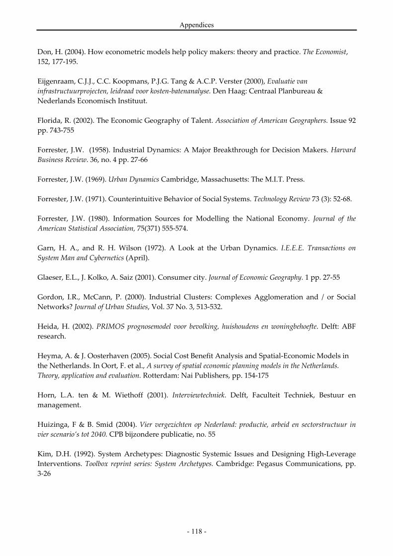
Appendices
- 118 -
Don, H. (2004). How econometric models help policy makers: theory and practice. The Economist,
152, 177-195.
Eijgenraam, C.J.J., C.C. Koopmans, P.J.G. Tang & A.C.P. Verster (2000), Evaluatie van
infrastructuurprojecten, leidraad voor kosten-batenanalyse. Den Haag: Centraal Planbureau &
Nederlands Economisch Instituut.
Florida, R. (2002). The Economic Geography of Talent. Association of American Geographers. Issue 92
pp. 743-755
Forrester, J.W. (1958). Industrial Dynamics: A Major Breakthrough for Decision Makers. Harvard
Business Review. 36, no. 4 pp. 27-66
Forrester, J.W. (1969). Urban Dynamics Cambridge, Massachusetts: The M.I.T. Press.
Forrester, J.W. (1971). Counterintuitive Behavior of Social Systems. Technology Review 73 (3): 52-68.
Forrester, J.W. (1980). Information Sources for Modelling the National Economy. Journal of the
American Statistical Association, 75(371) 555-574.
Garn, H. A., and R. H. Wilson (1972). A Look at the Urban Dynamics. I.E.E.E. Transactions on
System Man and Cybernetics (April).
Glaeser, E.L., J. Kolko, A. Saiz (2001). Consumer city. Journal of Economic Geography. 1 pp. 27-55
Gordon, I.R., McCann, P. (2000). Industrial Clusters: Complexes Agglomeration and / or Social
Networks? Journal of Urban Studies, Vol. 37 No. 3, 513-532.
Heida, H. (2002). PRIMOS prognosemodel voor bevolking, huishoudens en woningbehoefte. Delft: ABF
research.
Heyma, A. & J. Oosterhaven (2005). Social Cost Benefit Analysis and Spatial-Economic Models in
the Netherlands. In Oort, F. et al., A survey of spatial economic planning models in the Netherlands.
Theory, application and evaluation. Rotterdam: Nai Publishers, pp. 154-175
Horn, L.A. ten & M. Wiethoff (2001). Interviewtechniek. Delft, Faculteit Techniek, Bestuur en
management.
Huizinga, F & B. Smid (2004). Vier vergezichten op Nederland: productie, arbeid en sectorstructuur in
vier scenario’s tot 2040. CPB bijzondere publicatie, no. 55
Kim, D.H. (1992). System Archetypes: Diagnostic Systemic Issues and Designing High-Leverage
Interventions. Toolbox reprint series: System Archetypes. Cambridge: Pegasus Communications, pp.
3-26
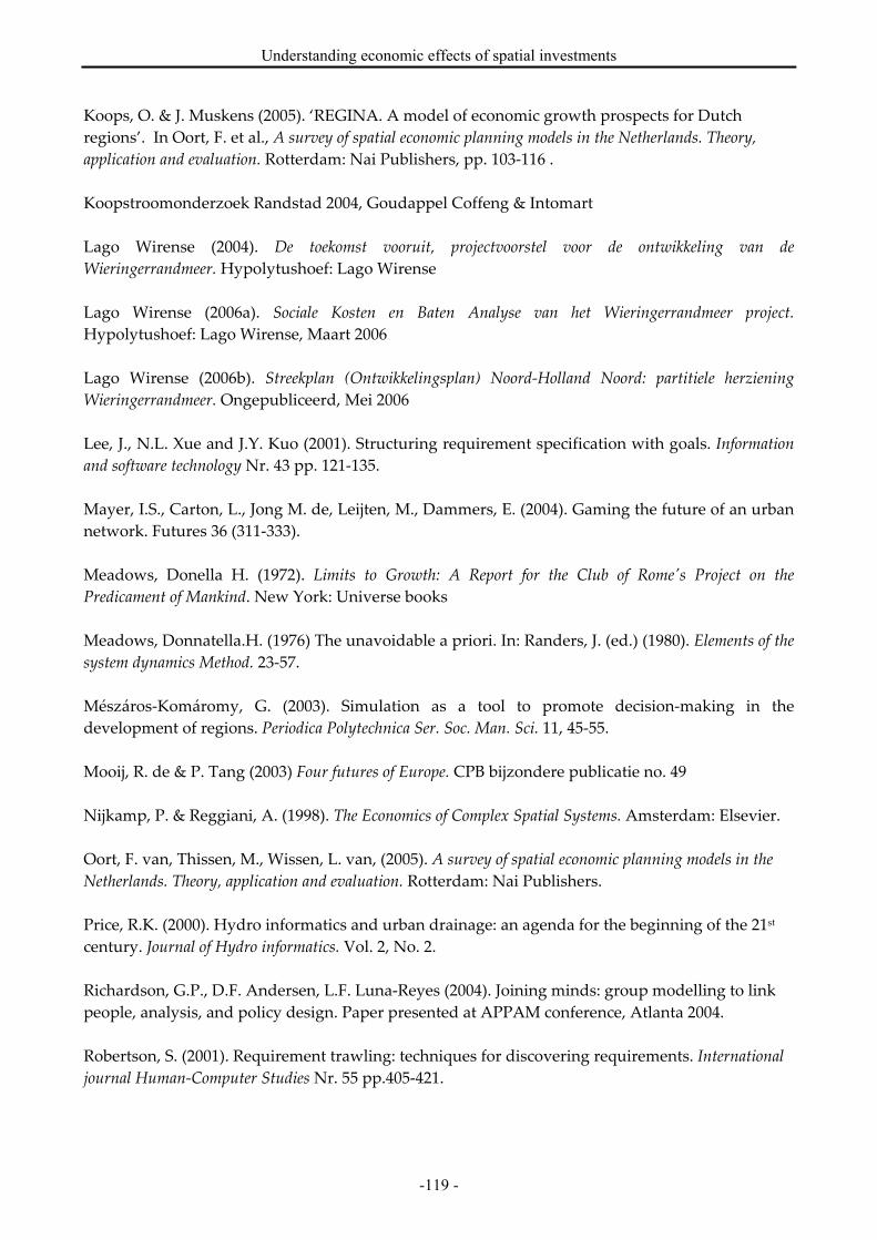
Understanding economic effects of spatial investments
-119 -
Koops, O. & J. Muskens (2005). ‘REGINA. A model of economic growth prospects for Dutch
regions’. In Oort, F. et al., A survey of spatial economic planning models in the Netherlands. Theory,
application and evaluation. Rotterdam: Nai Publishers, pp. 103-116 .
Koopstroomonderzoek Randstad 2004, Goudappel Coffeng & Intomart
Lago Wirense (2004). De toekomst vooruit, projectvoorstel voor de ontwikkeling van de
Wieringerrandmeer. Hypolytushoef: Lago Wirense
Lago Wirense (2006a). Sociale Kosten en Baten Analyse van het Wieringerrandmeer project.
Hypolytushoef: Lago Wirense, Maart 2006
Lago Wirense (2006b). Streekplan (Ontwikkelingsplan) Noord-Holland Noord: partitiele herziening
Wieringerrandmeer. Ongepubliceerd, Mei 2006
Lee, J., N.L. Xue and J.Y. Kuo (2001). Structuring requirement specification with goals. Information
and software technology Nr. 43 pp. 121-135.
Mayer, I.S., Carton, L., Jong M. de, Leijten, M., Dammers, E. (2004). Gaming the future of an urban
network. Futures 36 (311-333).
Meadows, Donella H. (1972). Limits to Growth: A Report for the Club of Rome's Project on the
Predicament of Mankind. New York: Universe books
Meadows, Donnatella.H. (1976) The unavoidable a priori. In: Randers, J. (ed.) (1980). Elements of the
system dynamics Method. 23-57.
Mészáros-Komáromy, G. (2003). Simulation as a tool to promote decision-making in the
development of regions. Periodica Polytechnica Ser. Soc. Man. Sci. 11, 45-55.
Mooij, R. de & P. Tang (2003) Four futures of Europe. CPB bijzondere publicatie no. 49
Nijkamp, P. & Reggiani, A. (1998). The Economics of Complex Spatial Systems. Amsterdam: Elsevier.
Oort, F. van, Thissen, M., Wissen, L. van, (2005). A survey of spatial economic planning models in the
Netherlands. Theory, application and evaluation. Rotterdam: Nai Publishers.
Price, R.K. (2000). Hydro informatics and urban drainage: an agenda for the beginning of the 21st
century. Journal of Hydro informatics. Vol. 2, No. 2.
Richardson, G.P., D.F. Andersen, L.F. Luna-Reyes (2004). Joining minds: group modelling to link
people, analysis, and policy design. Paper presented at APPAM conference, Atlanta 2004.
Robertson, S. (2001). Requirement trawling: techniques for discovering requirements. International
journal Human-Computer Studies Nr. 55 pp.405-421.

Appendices
- 120 -
RWS (2005). Basisboek instrumenten regionale bereikbaarheid: Rijkswaterstaat Adviesdienst Verkeer en
Vervoer, september 2005
Sanders F. & Sanders P. (2004). Spatial urban dynamics. A vision of the future of urban dynamics:
Forrester revisited. Unpublished.
SCP (2004). In het zicht van de toekomst: Sociaal en cultureel rapportage 2004. Den Haag: Sociaal
Cultureel Planbureau, 2004 (reeks Sociaal en Cultureel Rapport 2004).
Spector, J.M. (2000). System dynamics and interactive learning environments: Lessons learned and
implications for the future. Simulation & Gaming, Vol. 31 no.4 December 2000. pp. 509-516
Sterman, J.D. (2000a). Truth and beauty: validation and model testing. In J.D. Sterman (2000).
Business Dynamics: systems thinking and modelling for a complex world pp. 845-891.
Sterman, J.D. (2000b). Business Dynamics, Systems thinking and modelling for a complex world. London:
Irwin Professional.
TCI (2004). Tweede Kamer der Staten Generaal, Tijdelijke Commissie Infrastructuur-projecten.
Onderzoek naar infrastructuurprojecten. Sdu Uitgevers, ’s Gravenhage.
Thissen, M. (2005). RAEM: Regional Applied general Equilibrium Model for the Netherlands. In
Oort, F. et al., A survey of spatial economic planning models in the Netherlands. Theory, application and
evaluation. Rotterdam: Nai Publishers, pp. 63-84.
Toerisme Noord-Holland (2004). Activiteitenplan Toerisme Noord-Holland 2005 Amsterdam
Verkade , E. & W. Vermeulen (2005). The CPB labor market model. A tool for long-term scenario
construction. In Oort, F. et al., A survey of spatial economic planning models in the Netherlands. Theory,
application and evaluation. Rotterdam: Nai Publishers, pp. 45-62
Vermeulen, W. & J. van Ommeren (2005). Interaction of Regional Population and Employment:
Identifying Short-Run and Equilibrium Adjustment Effects.
Vermeulen, W. & J. van Ommeren (2006). Housing supply and the interaction of regional population and
employment. CPB Discussion Paper No. 65, May 2006
Verschuren, P. & H. Doorewaard (1999). Designing a Research Project. Utrecht: Lemma.
Vereniging van Nederlandse Gemeenten (2005). Oog voor Detailhandel. VNG uitgeverij, Den Haag.
Winsemius, P. (1986). Gast in eigen huis; beschouwingen over milieu management. Alphen a/d Rijn:
Samson.

Understanding economic effects of spatial investments
-121 -
Internet sources
www.CBS.nl
www.CPB.nl
www.RPB.nl
www.SCP.nl
www.VROM.nl
www.Wieringerrandmeer.nl

Understanding economic effects of spatial investments
- 122 -
8 Appendices
8.1 Appendix 1: List of definitions and abbreviations
Used definitions and abbreviations in this thesis.
CBS Statistics NetherlandsCOROP region Coordination Commission Regional Research Programme: Geographical
region larger than a municipality smaller than a provinceCPB the Netherlands Bureau for Economic Policy AnalysisDemographic pressure Ratio of inhabitants between 0 and 19 plus 65 and older and the working
labour forceDHV E&S DHV Economy and Space. A consultancy division of a large engineering firm
concerned with spatial economic problems. Emigration Departure from the Netherlands
Endogen variable A variable that is completely controled by the model
Exogen variable A variable that is not controled by the model but by an external data source
Fulltime equivalent All jobs (full and partime) calculated in full time equivalent units
Gross National Product Added value for market prices for the national economy.
Gross participation Percentage of labour force of total inhabitants
IER Integral Effect Study
Immigration Foreign settlement in the Netherlands
Industry sectors Deivision of all the of industries into a set of craft related sectors
Inhabitants Registered inhabitants on 31st of December
"Jip & Janneke" Making something overly simple
Job migration Migration to foreign country with the purpose of working there
Job An occupation in a specific industry sector
Labour productivity Total income derived from the production process devided by the total labour volume
Labour volume Number of fulltime equivalent units
Labour force Persons who work or want to work at least 12 hours per week
Level of participation Percentage of inhabitants 15-65 that participates in the job process
LER Aggriculture impact analysis
MER Environmental impact analysis
Migration surplus Balance between settlement from and to municipalities in the Netherlands
Model see simulation model
National migration surplus
Balance between settlement from and to foreign countries and the Netherlands
NEG New Economic Geography
Net participation Precentage of working labour force of total inhabitants
OEI (or OEEI) the Research program Economic Effect of Infrastructure PLC Policy life cycle
Policy maker Person responsible for and concerned with the development of projects from a government organisation
Population desity Inhabitants per square kilometre land
Population growth Birth and inland and foreign migration surplus
Production sectors see industry sectors
Resident-work balance Balance between jobs and potential labour force in the region
SCBA Social Cost Benefit Analysis
SCP The Social and Cultural Planning Office of the Netherlands
SD System Dyamics
SEES Social Econmic Effect Analysis
Simulation model Mathematical and visual representation of a real life system.
SMB Stratigic environment assessment
TCI Temporary Committee for Infrastructure projects
TNO the Netherlands Organisation for Applied Scientific ResearchUD Urban Dynamics

Master thesis – Teun Veldhuizen
- 123 -
8.2 Appendix 2: preparation for the requirement analysis
Appendix 2 contains a more detailed description of how the interviews in the requirement analysis
came about.
8.2.1 Dealing with different worldviews
Determining requirements is an important but sometimes underexposed phase in the design of
simulation models. The model is a translation of the real world, made through a series of
assumptions and simplifications by a model developer (Battjes et al. 2000). The model developer or
consultant sees the relation between the real world and simulation as a set of equations that
approximate the behaviour of the real system. The end-user of the simulation model, a policy
maker in this case, has a different worldview compared to the model developer (Checkland 1981).
Figure 9.1 illustrates the relation of these worldviews and the relation with the simulation model.
Figure 9.1, worldviews in model design
The consultant has to build a model that offers answers to the questions of policy maker. The
policy maker’s worldview is sunk in politics, previous engagements and deals and tension
between governments and political parties. A consultant cannot always be conscious of these
issues. A policy maker on the other hand is not conscious of issues that stem (for instance) from the
technical background of the software. Because of this lack of insight in each other’s worldviews
both consultants and policy makers will have to take part in the process of discovering
requirements. Another argument for including consultants and policy makers in the requirement
analysis is the fact that both are in fact users of the simulation model. The consultant uses the
model as means of providing a service for which a fee is charged, therefore the use the model as
way of generating income. The policy makers, who are at the receiving end of the consultants’
advice, use these services in order to come to better decisions.
Because requirements are often difficult to extract from policy makers and consultants, Robertson
(2001) identifies three types of requirements that have to be addressed in order to get an (nearly)
exhaustive list of requirements. She considers:
• Conscious requirements: this is the set of requirements the stakeholder or client is most aware of.
This awareness is directly linked to the worldview of the client and often stems from the
Simulation model
Real world
Consultant (model
developer )
Policy maker (model user )
Dealing with worldviews

Understanding economic effects of spatial investments
- 124 -
reason for building a new product. An example: the simulation model must be able to run
different (economic) scenarios.
• Unconscious requirements: the stakeholder does not mention unconscious requirements because
he or she implicitly assumes the product will fulfil a particular function or have a particular
attribute. This problem is intensified when a stakeholder is informed about the product and
makes assumptions concerning the new product based on his existing knowledge. Robertson
mentions that it is often politeness that causes people to not name certain requirements,
because they do not want to patronize their interviewer. An unconscious requirement for the
simulation model may be that people expect that it incorporates validated data from the
Statistics Netherlands.
• Undreamed requirements: requirements that are not pointed out because either the stakeholder
thinks that it is impossible to incorporate an idea or function. Or the stakeholder is totally not
aware of a certain function that the product could possess. Finding these requirements is more
complex; an end-user is often not able to identify undreamed requirements. It is therefore
important to trawl for requirements in combination with technical analysts and model experts
too. An example for the simulation model that could only have come from another model
expert is the introduction of regression analysis on the relation between the input and output
variables.
In order to overcome these problems multiple sources of requirements have to be used:
consultants, policy makers and model experts. In the next section several techniques for
requirement trawling are introduced.
8.2.2 Why use interviewing as a requirement trawling technique?
There is a broad spectrum of instruments and methodologies for finding requirements for a new
product or service. Some instruments are better suited for finding conscious requirements, while
others have a larger potential for finding undreamed requirements. The list below shows a short
list of techniques that can be considered for the extraction of requirements for the simulation
model.
• Brainstorming: probably the best-known technique for generating a lot of ideas in a short time is
brainstorming. Many variations exist, some very informal with sticky notes, others very
systematic using computer aided techniques. Brainstorming is especially good for finding
undreamed requirements because creativity is stimulated and no time is given for evaluation.
A successful brainstorm should however comply with a few rules: the group members should
have diverse backgrounds, no criticism is allowed during the session and seemingly extreme or
crazy ideas are very welcome. The ideas should furthermore be snappy and short and be
combined or improved by others (Cross, 2000).
• Interviewing: interviewing is probably the most applied technique for discovering
requirements. It is an instrument for identifying conscious requirements from experts and
stakeholders. By interviewing different actors and different experts a holistic view of the
requirements is obtained. Due to the explorative nature of requirement trawling most
questions should be open to stimulate creative answers and the discovery of new requirements
(Horn, 2001). However closed questions are useful when looking for “maximum” or
“minimum” requirements.
• Mind mapping: a technique for graphically recording thoughts and ideas. By using words,
drawings, colours and symbols requirements can be easier identified, as more information is

Master thesis – Teun Veldhuizen
- 125 -
stored. Mind mapping is generally good for discovery of conscious, unconscious and
undreamed requirements. The disadvantage of mind mapping is that drawings are harder to
interpret at a later time (Cross, 2000).
• Reusing requirements: reusing requirements it not so much a technique as it is an often-
overlooked source of requirements. For the development of software and specialized instances
of this software (applications) that have been developed in a consistent manner, some
requirements can be reused. However, in the development of simulation models the practice of
creating a list of requirements in less common and it is therefore hard to reuse requirements for
this specific thesis model (Cross, 2000).
• Use case workshops: a use case workshop approach stems from soft systems thinking and is a
way of observing the world in order to understand it. In a use case workshop a functional part
of a system is tested with a group of end users or experts. Translated to the simulation model
this would mean that a partly finished model is tested on some of its functional requirements.
As nearly all of the end users are not familiar with working with simulation models this could
prove to have two results. First, in a use case workshop functions can be tested like adding a
new variable to the model or changing the value of a variable. This way the use case workshop
also tests the model. The second result a use case workshop has is that it familiarises end users
with the simulation model and it offers a good opportunity to show the structure and inner
workings of the simulation model. During a use case workshop especially unconscious and
conscious requirements are found (Cross 2000).
For the thesis model interviewing has been chosen as requirement trawling technique. Interviews
can be executed from remote locations via telephone; furthermore they do not (as work shops do)
require complex meeting arrangements or long introductions. The interviews follow an open line
of questioning to promote the respondent to think of unconscious and undreamed requirements.
Interviewing is also the best way to reach respondents that are situated at different locations, as
group brainstorms require all people to be in the same room. Some interviews with policy makers
and consultants who were familiar with model building resulted in discussions and brainstorms
about the requirements the model should have.
For the reuse of requirements, old lists of requirements had to be found first. As it appeared that
requirements of simulation models are not structurally recorded, no reusable lists were found. A
final reason for not using case workshops in the requirement analysis is that this technique
requires part of a finished simulation model for demonstration. However a use case workshop
where end-users will be able to work with the model is scheduled during phase 4 of the thesis
project, when the model is partly finished (as described in section 4.2.2).
8.3 Appendix 3: Questionnaires
Appendix 3 provides the policy maker and consultant questionnaires that have been used in the
requirement analysis. These questionnaires are in Dutch because the respondents were all Dutch
native speakers.
8.3.1 Policy maker Questionnaire
1. Bent u wel eens in aanraking gekomen met beleidsondersteunende modellen?
a. Ja (vraag 2-5)

Understanding economic effects of spatial investments
- 126 -
b. Nee (vraag 6)
2. In welke omgeving heeft u deze modellen gebruikt
a. Als “modelbouwer”
b. Gebruiker van resultaten: op welke manieren zijn de resultaten gebruikt
3. Kunt u een doel aangeven van door u gebruikte beleidsondersteunende modellen
a. Financiële haalbaarheid
b. Genereren van alternatieven
c. Maken van planning
d. Anders…….
4. Kunt u aangeven in welke fase van het beleidsproces de beleidsondersteunende modellen
gebruikt werden? (figuur 1)
Figuur 1, de policy life cycle
Korte uitleg over de interpretatie van beleidsondersteunende modellen in het
afstudeeronderzoek
Dimensie 1) Communicatie
5. Hoe ziet u het liefst de resultaten gepresenteerd tijdens een (groeps)presentatie?
a. Grafieken met tijdsverloop (1 of meerdere variabelen)
b. Histogrammen (1 of meerdere variabelen)
c. Plaatjes (foto’s, diagrammen)
d. Tabellen (meerdere variabelen)
e. Anders…..
Aan welke eisen zou het besluitvormingsmodel moeten voldoen mbt tot presentatie van
uitkomsten?
6. Is in uw opzicht een basaal begrip van een beleidsondersteunend model nodig voor het op
juiste wijze gebruiken van de uitkomsten?
a. Zo ja, in hoeverre?
b. Zo nee, waarom niet?
c. Zou u dat wel willen hebben?
7. Welke indicatoren zijn het meest belangrijk bij het nemen van een beleidsbeslissing?
(financiële haalbaarheid, werkgelegenheid, bestedingen, inkomen, voorzieningen, forensisme)
8. Hoe worden deze indicatoren op het moment berekend?
9. Stelt u eisen aan de duur van een sessie waarbij het simulatiemodel optreedt als instrument in
de discussie?
Dimensie 2) Model performance
10. Hoe gebruik u doorgaans de informatie uit onderzoeken?
a. Gebruik gemiddelde waarden
(1) Probleem herkenning
(3) Bekleids-implementatie
(2) Beleids-formulering
(4) Controle van beleid
Probleem

Master thesis – Teun Veldhuizen
- 127 -
b. Gebruik gemiddelde waarden en standaard afwijking
c. Gebruik gemiddelde waarde en gevoeligheidsanalyse
d. Gebruik van uiterste waarden (economische scenario’s)
Welke eisen stelt u aan de informatie uit onderzoeken met betrekking tot het bovenstaande?
11. Aan welke aspecten wordt aandacht besteed bij het gebruiken van onderzoeksresultaten in
besluitvorming?
a. Bij steekproeven: de representativiteit van de genomen steekproef
b. Bij model gebruik:
1. Compleetheid van het model
2. Juistheid van de modelstructuur
3. Onzekerheid gebruikte aannames
12. Hoe zou met bovenstaande aspecten moeten worden omgegaan en hoe kan een model daarbij
aan bijdragen? (indicatie van bounds)
13. Hoe worden “zachte” gegevens vertaald in “harde” data?
Dimensie 3) Probleem setting
14. Als in het beleidsproces model(uitkomsten) worden gebruikt, waartoe dienen deze dan?
a. Het verkrijgen van goedkeuring van een hoger gelegen overheid
b. Verantwoording afdragen richting de burger
c. Het creëren van draagvlak bij burgers
d. Het creëren van draagvlak bij andere overheden in het algemeen
e. Het creëren van draagvlak bij andere politieke partijen in uw overheidssetting
Welke eisen aan het model komen hieruit voort?
15. In hoeverre geven modeluitkomsten doorslaggevende bewijs in besluitvorming? Probeer een
percentage aan te geven 0 – 100%? Waar hangt dit vanaf?
16. Stel u geeft de opdracht tot het uitvoeren van een economische studie naar de effecten van een
ruimtelijke investering. Wat zijn de belangrijkste eisen die u stelt? (Inzicht in modelstructuur,
betrouwbaarheid, uitkomst richting…)
17. Als we het hebben over schaalniveaus van problemen waarvoor een economische effect studie
wordt uitgevoerd waar ligt dan de:
a. Geografische schaal?
b. Financiële schaal?
c. Tijdschaal?
18. Hoe worden verschillende scenario’s gebruikt in de besluitvorming?
a. Economische scenario’s
b. Verschillende beleidsalternatieven
8.3.2 Consultant Questionnaire
1. Bent u wel eens in aanraking gekomen met beleidsondersteunende modellen?
a. Ja (vraag 2-5)
b. Nee (vraag 7)
2. In welke omgeving heeft u deze modellen gebruikt
a. Als “modelbouwer”
b. Gebruiker van resultaten: op welke manieren zijn de resultaten gebruikt
3. Kunt u een doel aangeven van door u gebruikte beleidsondersteunende modellen
a. Financiële haalbaarheid
b. Genereren van alternatieven

Understanding economic effects of spatial investments
- 128 -
c. Maken van planning
4. Kunt u aangeven in welke fase van het beleidsproces de beleidsondersteunende modellen
gebruikt werden? (figuur 1)
Figuur 1, de policy life cycle
5. Gebruikte u ook een lijst met ontwerpeisen bij het ontwikkelen van deze modellen? Zo ja,
welke eisen waren dit? (Reusing requirements)
Korte uitleg over de interpretatie van beleidsondersteunende modellen in het
afstudeeronderzoek
Dimensie 1) Communicatie
6. Waar geeft u de voorkeur aan bij het presenteren van resultaten uit onderzoek bij klanten in
een presentatie?
a. Grafieken met tijdsverloop (1 of meerdere variabelen)
b. Histogrammen (1 of meerdere variabelen)
c. Plaatjes (foto’s, diagrammen)
d. Tabellen (meerdere variabelen)
Aan welke eisen zou het besluitvormingsmodel moeten voldoen mbt tot presentatie van
uitkomsten?
7. Met welke interface zou u kunnen aankomen bij een klant? En waarom
a. Spreadsheet / MS Excel
b. SD � Vensim
c. SD � Powersim
Aan welke eisen zou het besluitvormingsmodel moeten voldoen mbt tot de user interface richting
de consultant?
8. Is in uw opzicht een basaal begrip van een beleidsondersteunend model nodig voor het op
juiste wijze gebruiken van de uitkomsten?
a. Zo ja, in hoeverre?
b. Zo nee, waarom niet?
Welke eisen komen hieruit voort?
9. Hoe kan inzicht in het model in uw ogen bijdragen aan betere beslissingen?
Kunt u hier ook functionele eisen aan verbinden?
10. Stelt u eisen aan de duur van een sessie waarbij het simulatiemodel optreedt als instrument in
de discussie?
11. Zijn er nog overige eisen met betrekking tot communicatie?
Dimensie 2) Model performance
12. Welke informatie uit onderzoeken levert u doorgaans aan de klant?
(1) Probleem herkenning
(3) Bekleids-implementatie
(2) Beleids-formulering
(4) Controle van beleid
Probleem

Master thesis – Teun Veldhuizen
- 129 -
a. Gemiddelde waarden
b. Gemiddelde waarden en standaard afwijking
c. Gemiddelde waarde en gevoeligheidsanalyse
d. Uiterste waarden (economische scenario’s)
Welke informatie zou het model moeten kunnen produceren?
13. Is het belangrijk dat model variabelen kunnen worden aangepast en real time kunnen worden
uitgerekend (lees: bij de klant)?
o Wat is de maximaal toelaatbare tijd voor deze berekening?
14. Binnen welke tijd zou een model door een consultant gemaakt moeten kunnen worden? (wat is
gebruikelijk?)
15. Welke eisen zou u kunnen formuleren met betrekking tot het performance aspect van
beleidsondersteunend model zoals besproken?
Dimensie 3) Probleem setting
16. Als in het beleidsproces model(uitkomsten) worden gebruikt, waartoe dienen deze dan?
a. Het verkrijgen van goedkeuring van een hoger gelegen overheid
b. Verantwoording afdragen richting de burger
c. Het creëren van draagvlak bij burgers
d. Het creëren van draagvlak bij andere overheden in het algemeen
e. Het creëren van draagvlak bij andere politieke partijen in uw overheidssetting
17. In welke fase wordt DHV in de meeste gevallen betrokken bij een besluitvormingsproces waar
modellen gebruikt worden.
Welke eisen komen hieruit voort?
18. Bij het uitvoeren van een project voor een klant wat is dan de toegevoegde waarde van een
model voor een klant
• Inzicht in modelstructuur en daarmee inzicht in de gevolgen van besluitvorming
• Bevestiging van een vooraf ingenomen standpunt (steun dmv model)
19. Als we het hebben over schaalniveaus van problemen waarvoor een economische effect studie
wordt uitgevoerd waar ligt dan de:
e. Geografische schaal?
f. Financiële schaal?
g. Tijdschaal?
Welke eisen komen hieruit voort?
8.4 Appendix 4: Lists of interviewees
This appendix shows the respondents that have been interviewed for different parts of the thesis
project: the requirement analysis, the groups testing sessions and the expert validations.
Interviews for the requirement analysis
Name Function Date
P. Canisius Senior consultant at DHV Management Consultants 17-11-2005
E. van Daalen System Dynamics expert at the faculty of Technology, Policy
and Management of the Technical University of Delft
04-01-2006
M. Pellenbarg Consultant at DHV Economy and Space 16-12-2005
B. Schilder Risk expert at DHV Management Consultants 19-12-2005

Understanding economic effects of spatial investments
- 130 -
P. Smolders Strategic consultant at DHV Economy and Space 25-11-2005
A. Stegeman Project coordinator at Lago Wirense PMT 23-12-2005
M. Thissen Regional economic models expert at the National Institute
for Spatial Research
20-12-2005
H.
Timmermans
Strategic consultant at DHV Economy and Space 14-11-2005
J.P. Vis Former municipal council member of the city of Delft 21-12-2005
W.
Voordenhout
Senior financial economic policy maker at the province of
North-Holland
13-12-2005
Interviews for the group testing sessions
Name Function Date
M. van Andel SEPAM graduate student 03-04-2006
E.J. van Stijn SEPAM graduate student 03-04-2006
M. Pellenbarg Consultant at DHV Economy and Space 26-04-2006
H.
Timmermans
Strategic consultant at DHV Economy and Space 26-04-2006
E. Bos Eyssen Junior consultant at DHV Economy and Space 26-04-2006
M. Embregts Junior consultant at DHV Economy and Space 26-04-2006
C. Raijmakers Project manager at DHV Economy and Space 26-04-2006
S. Wilmink Consultant at DHV Management Consultants 05-05-2006
R. Derks Consultant at DHV Investment Services 05-05-2006
P. Canisius Senior consultant at DHV Management Consultants 05-05-2006
Interviews for the expert analysis
Name Function Date
B. Schilder Risk expert at DHV Management Consultants 16-05-2006
F. van Oort Professor at the University of Utrecht 16-06-2005
A. Stegeman Project coordinator at Lago Wirense PMT 10-05-2006
M. Thissen Regional economic models expert at the National Institute
for Spatial Research
15-06-2006
H.
Timmermans
Strategic consultant at DHV Economy and Space 16-05-2006
W. Vermeulen Researcher at the CPB 12-05-2006
W.
Voordenhout
Senior financial economic policy maker at the province of
North-Holland
23-05-2006
8.5 Appendix 5: Policy maker questionnaire long list
This appendix gives an overview of the answers given during the interviews with the consultants
and policy makers. Because a lot of information was given during the interviews that did not fit
into the format of the line of questioning each subject that is discussed starts with some general
insight on the subject.

Master thesis – Teun Veldhuizen
- 131 -
8.5.1 Results from the policy maker questionnaire
General insights
• A (financial) model is always used in policy making as long as it contributes to the final goal
(project realisation)
• A model should (if possible) accommodate the dynamics of the policy process. Policy goals
change over time
• For smaller communities experience and common sense more important than a model
• The model should make clear what the socio-economic effects would be if the project is
stopped before the final phase. (WRM stopped after phase 3 of 5)
• The politisation of a policy proposal is extended as long as possible
• Previous model user
o Yes (2)
o No (2)
• Important goals of policy supporting models
o Financial feasibility (2)
o Risk analysis on investments (0) * (providing some form of assessment)
o Providing “hard” information in uncertain environments (1)
o Applying standardized methods on different cases for comparison (1)
o Generating alternatives (1)
• Policy phase for model use
o Problem recognition
� Phase one is in the RO business mostly lobbying
o Policy formulation (1) *
� Translation of policy goals into policy alternatives
� Providing insight towards “management”
� Zuiderzeelijn � a war that is fought with reports and research
o Policy implementation (2)
� Delft urban master plan
o Policy evaluation is gaining ground, subject disserves more attention (1)
Dimension 1) Communication:
General insights
• Policy makers prefer graphs and visual images in presentations, more information (tables etc.)
should be available in the project report.
• Make difference in presentation style for different groups: always interactive but the amount of
interaction should depend on how deep you wish to go a specific subject
o Policy makers: lots of possibilities to change variables and assumptions
o B&W: present a few alternative (complete solutions) only a few possible variable
changes
o Counsel (de raad): present only one option, they will either appose or approve
• “Local heroes” are more important in small communities and have to be accounted for.
• Level of specialism in small communities not high, make sure the model can depict very basis,
simple things and practical examples.

Understanding economic effects of spatial investments
- 132 -
• The timing of the use of the model is crucial; if the PM’s are not familiar with the method they
will reject it.
• Putting multiple actors in one room with the simulation model might pose a threat; the model
will only be used as a political argument.
• Don’t forget that policy decision always revolve around 1 alternative and that policy making
always on multiple alternatives.
• Presentation style
o Tables (1)*
� In report
o Graphs (3)*
� Provides quick overview
� Is not too complex
� Histograms useful
o Visual images can support the project (presentation Piet v. Hemmen) policy makers can
identify easier with visual images. (Politicians are dreamers who think in images) (2)
o Always keep your audience in mind
o Cartoon like (stripverhalen versie)
o Mix it up
• Interface:
o Excel ok because familiar
o Causal relations only to explain principles of model
o Model must suit the user group
o Model must be able to support the gut feeling that people have
• Understanding of model by policy makers
o Yes, but only some basic principles, no math. Give short 5-minute introduction on the
principles of SD � emphasis on causal relation and stock and flows.
o You do not want this; only use very rudimentary practical examples to illustrate the
method that you use.
o No theory!
o Depends on the policy phase: in a final decision-making phase there is no need for
understanding the model, decision makers want (hard) numbers. If a decision needs to
be made on what alternative to chose, some understanding is needed
• Important indicators for policy decisions
o Housing market
o Inhabitant
o Employment (especially for WRM) (2)
• (Show relation between these three)
o Consumer purchasing power
o Make explicit: low income + low employment = bad (disadvantaged area); high income
+ low employment = good (retired empty nesters with good pension)
o Make difference in municipalities (Wieringen, Wieringermeer)
o Effects of tourism
• (Relay the outcomes of the Alterra report)

Master thesis – Teun Veldhuizen
- 133 -
o Economic trends and growth
o Show 4 year political cycles
• How are the important indicators measured
o See above
o Hard numbers always win from soft words
o If gut feeling not supported with any of the indicators, the model is rejected
• Time span of interactive session with simulation model
o Not longer than two hours
o Depends on the policy phase (2)
o Brief the different political parties first and work with them first before combining
multi actor groups
o
Dimension 2) Performance:
• General notions
o Always check if the all the model variables are included in the specific case
o Politicians use common sense and base their decisions on their own common sense.
(Example: 5% growth for 10 years is implausible) (3)
o Information from external firm has twice the impact than internal information!! (3)
o Think on “dakkapellen” niveau
o Depending on the phase of the policy process different requirements are needed. When
the policy is just forming you will want to see the effects of different policy alternatives
for a specific problem. In a later phase when decisions will need to be made, a model is
necessary that will only show 1 alterative with different economic scenario’s
• Information format: what types of information are communicated towards the client
o Average (2) always *
o Average and st. dif (2) if necessary
• Hardly ever
o Average and sensitivity analysis (1) *
• Forms the basis of decision making, is always communicated “up”
• Never (1)
o Scenario analysis (1)
• Most of the time only scenario’s
o The use of cold numbers is the most common, stick with it
• Dealing with uncertainty
o Always communicate assumptions (3) *
• Should be present and clear
o When model is a big mess (“brij”) policy makers cannot find the steering points! When
the model is a brij it is perceived as uncertain
Dimension 3) Problem setting:
General insights:
• Research costs are not intended to be proportional to the investment. It largely depends on the
political position of the project.

Understanding economic effects of spatial investments
- 134 -
• If citizens are against and investment the municipal counsel will follow this trend.
• First approach people individually and find out what their “real” problem is.
• Use of model outcomes for:
o Getting approval from higher government (1)
� Not often but does happen
� Used to create commitment
� Yes does happen province and national government
o Responsibility towards residents (1)
� Almost never happens
� Yes can happen
o Creation of support towards residents (2) *
� Very important in municipal setting
� Most important!
� Make clear to the local heroes that this project is important, they will pull other
people in agreeing as well
o Creation of support towards other governments (2) *
� Promotes cooperation between local governments
� Delft � most important
o Creation of support towards other political parties (1) *
� Very important! Persuading countering parties
� This does not have to happen with a model; usually it is caused by the lack of
political support.
• How much do model outcomes influence policy decisions
o 60% but never decisive
o Lobby is sometime more important
o In WRM different per municipality: Wieringen is very sceptic and will not bow for a
model. In Wieringermeer they will use the model in their advantage (70-80%)
o When a plan has already been made the political will is dominant.
o In early phase of policy making the effect can be large
• Most important demands (requirements) for client
o Not model structure insight! (1)
o Reliability (2)
• Providing knowledge on reliability
• Is a given, right?!
o Direction of outcome very important
• Reports do not get published if outcomes does not support the project
o Has to be able to work with different groups on different levels
o Economic prospects
o Show difference between different studies, why do they have different outcomes.
• Choice of scale
o Geographical scale
• Province (2)
• Between smaller municipalities (1)

Master thesis – Teun Veldhuizen
- 135 -
o Financial scale
• Larger than 10 million (1) *
• Depending on political climate (1)
o Time scale of outcomes
• < 30 years (2) *
• How are scenario’s used in policy making
o As reference (2)
o Provides perspective (2)
• Also plays role in the dual system and distributed responsibility
o Always a combination of economic scenario and policy alternatives
8.5.2 Results from the policy maker questionnaire
• General insights
o Simple models are better
o Cash flow models are relatively simple compared to mechanical fluid models (technical
background is pro in consultant)
o MKBA is more a method not so much a model
o A model should give:
• Insight in problem and solution(s) --> knoppen draaien
• Overview of the problem --> what is the real problem and what is its root
o Policy makers are not used to working with models: reduce complexity that is
presented to them to a minimum.
o Agreements on representation of outcomes and mathematical methods (risk analysis)
• Previous model user
o Yes (3)
o No (2)
• Most important goal of policy supporting models
o Creating insight (2) *
o Financial feasibility (2) *
o Giving more information that just a yea/no answer (2)
o Giving support in reaching the end goal. What should change to meet the desired
results (1)
o Providing insight in project risks (1)
• Policy phase for model use
o Policy formulation (4) *
� Should we make the investment
� Formulation of alternatives
� Is the investment justified
� Why are alternatives more expensive
� Weighing risks of alternatives
o Policy implementation (1)
� Risk cost calculation
o Policy evaluation is gaining ground, subject disserves more attention (1)

Understanding economic effects of spatial investments
- 136 -
• Reuse of requirements
o Requirements? (3)
o Does not happen in practice very often (2)
Dimension 1) Communication:
General insights
• Policy makers should make an effort in reading tables, they always want graphs.
• Presentation style
o Tables (3)*
� Most information in least amount of space
� Often harder to interpret
o Graphs (3)*
� Easy to misinterpret
� Histograms
� Distributions of uncertainty of variables
o Indication what are the causes of large model changes (1)
o Indication of relation between input and output has to be clear (1)
o Less information on more sheets is better that lots of information on one sheet (1) * -->
not more than 6 items on sheet?
o Not more than 2 or 3 variables in table or graph
o Not more that 4 variables in table
o By providing insight in the risks of a project and the magnitude of these risks, decisions
are made on a broader base than only seeing estimations.
• Interface:
o Preferably only input-output (1)
o Not too much graphs and pictures (too messy) (2)
o Stella notation is useful (1)*
o Very clear overview of assumptions should be available (2) *
o Separate (but prominent) sheet with assumptions
o Excel: is the most familiar for users
• Understanding of model by consultant
o It is important that the consultant knows how the model works and has very basic
understanding of system dynamics (2) *
o It should not be necessary to be a SD expert to use the model or to fully understand the
mathematical background (3)
o A very good (practical) guideline PowerPoint presentation should be enough for the
consultant to be able to work with the model (2) *
o Make a difference in what a model builder should know and what someone would
have to know who only presents the results at the customer (1) *
• Other

Master thesis – Teun Veldhuizen
- 137 -
o Communication of assumptions towards customer very important. Especially highly
sensitive assumptions and assumptions with high impact. (3) *
o Don’t make the interface too complex --> provide information in the programme --> a
help function
Dimension 2) Performance:
• Information format: what types of information are communicated towards the client
o Average (4) always *
o Average and st. dif (1) almost never *
o Average and sensitivity analysis (3) does not always happen, but should be done *
o Scenario analysis (2) is almost always part of assignment
o Boundaries of outcomes are very important (2)
o Boundaries 100*µ
σ and reliability interval (1)
• In costing: 30% boundary space in early phases is allowed in later phases this is
about 5% depending on the project.
• Other model information
o Correlation between assumption values and outcomes
o Dependence between assumptions and policy variables (2)
o Relations between policy variables and important factors *
o Feedback loops *
o Performance indicator of results for specific region compared to other geographical
units
• Model realisation time
o Unknown (2)
o One day is allowed (2)
o One minute *
• Other demands
o Indication of bounds (3)
o Indication of model accuracy (= bounds?) (2)
o Calculation of uncertainty with independent variables � giving the lower uncertainty
bound
o Calculation of uncertainty with dependent variables � giving the upper uncertainty
bound (you need to group your variables in depended groups)
Dimension 3) Problem setting:
General insights:
• Are research costs proportional to the project? Is there some sort of “staffel”?
• Research should foremost be executed to create clarity in fuzzy situations.
• The specific use of the model can be attributed to a specific phase in policy making. Not every
model is suited for every policy phase.
• Use of model outcomes for:

Understanding economic effects of spatial investments
- 138 -
o Getting approval from higher government (1)
� Compare policy options (2) *
o Responsibility towards residents (2)
� Model outcomes will have to be translated into “Jip & Janneke” language (3) *
o Creation of support towards residents (1)
� Turning no into yes in society
o Creation of support towards other governments
o Creation of support towards other political parties (2) *
• In which phase is DHV involved in the policy making process
o All phases (3)
o The model should accommodate searching for alternatives and testing predefined
alternatives (1) *
• Added value of model for client
o Providing figures on the consequences of the policy decision (1) *
o Confirmation of predetermined standpoint (the model gives backup) (2)
• Would like “intended” outcomes, but under specific conditions.
o Providing insight in how to make a project profitable/acceptable (1) *
• Providing “mitsen en maren”: project plan is only feasible if … and …
• Choice of scale
o Depending on phase of project, early phases the scale can be very large. Later phases
more specific and precise information is needed and therefore the focus will become
smaller or your model will grow larger.
o Geographical scale
• Difficult due to distributive effects (1)
• Depends on client and the intentions of the client (gain support etc)
• Make clear choice why you do / don’t take effects in adjacent regions into
account (2) *
o Financial scale
• Unknown
• Larger than 10 million (2)
• Research costs as percentage of investment costs
o Time scale of outcomes
• Different per project (2)
• 10 – 20 years (2) *
30 years (1) *
8.6 Appendix 6: The final requirement lists
This appendix shows the final lists with requirements and is the end result of the requirement
analysis. The requirements that are vital for the simulation model are indicated as a “Need to
have” requirement. All the other requirements can be regarded as “nice to have”. The column “In
model” indicates if a requirement is implemented in the final simulation model. The requirement
lists are presented per respondent group:

Master thesis – Teun Veldhuizen
- 139 -
• 8.6.1: the policy makers
• 8.6.2: the consultants
• 8.6.3: the policy issue
• 8.6.4: the literature study
8.6.1 The final requirement list of the policy makers
Communication: policy maker Need to have In model
• Present results in graphs and histograms Yes Yes
- Maximum of 2 variables per graph Yes Yes
- Use tables only in final report, not in presentation Yes Yes
• Present results in MS excel format No Not realtime
• Present results in cartoon like fashion No No
• Be able to change presentation “styles” from comprehensive to simple Yes Yes
- Two or three interfaces with different levels of detail Yes Yes
- A “Jip en Janneke” version explainable to laymen Yes Yes
• Not require more than 5 minutes on theory of system dynamics Yes Variable
• Must be able to adapt to the capricious political arenas No No
• The interactive session must not take longer than an one day part (4
hours)
No Variable
• The interactive session must not take longer than 2 hours No Variable
• Be as simple as possible strive to still complex
- Have as least variables as possible strive to 75
• Include the following factors
- Housing market Yes Yes
- Inhabitants Yes Yes
- Employment Yes Yes
- Show relation between housing market, inhabitants, employment Yes Yes
- Consumer purchasing power No No
- Effects of tourism Yes Yes
- Show 4 year policy cycles No No
- Economic trend and growth Yes Yes
• Interpret the combination of two factors (for instance high income, low
employment)
No No
Performance: policy maker Need to have In model
• Include variables that are specific to a region Yes Yes
- Allow to add or remove variables depending on situation Yes Yes
• Support common sense reasoning Yes Yes- What if questions Yes Yes
• Only use averages No Yes + extra• Not give information on variable bounds No No• Give information on variable bounds Yes Yes
• Offer the possibility to calculate different scenarios Yes Yes
• Present uncertainties and assumptions in complete but orderly fashion. Yes Yes
• Communicate reliability (outcomes are of model often instantly accepted
and used)
Yes Yes
• Provide clear description of status of model outcomes Yes Yes

Understanding economic effects of spatial investments
- 140 -
8.6.2 The final requirement list of the consultants
Policy issue: policy maker Need to have In model
• Be preceded by session that will give people some information about
what they can expect of the simulation model
Yes Yes
• Support gut feeling of policy makers No Yes
• Communicate to the following groups:
- The residents of a region (they will influence local government) Yes Yes
- Other governments (for the creation of support) Yes Yes
- Other political parties for the (creation of support) No Yes
• Connect to the lobby efforts (Lobby can be very important) No No
• Be used in early phase of policy life cycle Yes Yes
• Show differences between different studies on same subject No No
• Give indication of effects on provincial scale No No
• Give indication of effects between small municipalities No No
• Be suited for projects that have a financial scale large then € 10 mln. Yes Yes
• Show result on a time scale between < 30 years Yes Yes
• Use scenarios for reference and perspective (should always be a
combination of economic scenarios and policy alternatives)
Yes Yes
• Show what happens if the project is stopped during one of the phases (A
project is often divided into phases)
Yes Yes
Communication: consultant Need to have In model
• Be suited for the use with different actors Yes Yes
- Two or three interfaces with different levels of detail Yes Yes
• Facilitate policy evaluation No No
• Present results in tables Yes Yes
- Maximum 4 variables in one table (max 3) (max 3)
• Present results in graph Yes Yes
- Maximum 3 variables in one table (max 3) (max 2)
• Not have a complex interface Yes Yes
- Max 6 adjustable variables on one screen (max 6) (max 2)
• Show relationship between input and output variables
- Display input and output variables in same window strive to Yes
- Display effects of steering variables on important factors Yes Yes
• Provide a clear overview of the (relevant) model assumptions Yes Yes
- More attention for sensitive assumptions No Yes
• Have a help function included No Yes
• Be accompanied by user guide for consultants (PowerPoint presentation) Yes Yes
• Have an A4 explaining the model principles for layman Yes Yes• Show visual representation of model relations Yes Yes

Master thesis – Teun Veldhuizen
- 141 -
Performance: consultant Need to have In model
• Only display average results No No• Display other information only on request Yes Yes
- Standard deviation of outcomes Yes No
- Indicate Sensitive variables Yes Yes
- Reliability interval Yes Yes- Indication of bounds of reliability interval Yes Yes
- Feedback loops (graphical) Yes Yes
• Show a distribution of uncertainty in output variables Yes Yes
- Run model with independent stochastic input variables (lower
uncertainty bound)
Yes Yes
- Run model with dependent stochastic input variables (upper uncertainty
bound)
No No
• Give clear indication of sensitive variables Yes Yes
- Perform sensitivity analysis Yes Yes
- Give sensitive variables special colour No No• Show dependence between assumptions and policy variables No Yes
• Performance indicator of results for a specific region compared to other
geographical units
Yes compared to netherlands
- Display similar factors from inside and outside the region Yes (not all)• Adjust steering variables and calculate new results within 24 hours. Yes √ (5 seconds)
• Make use of the known models and modelling techniques Yes Yes
- Shift-Share analysis Yes Yes
- Housing market models Yes Yes
• Make use of existing methodology ad theories Yes Yes
- OEEI Yes Yes
- New Economic Geography Yes No
• Be reproducible Yes Yes
- Provide list with model equations Yes Yes
- Provide all input factors Yes Yes
• Store outcomes of important factors in spreadsheet Yes Yes
Problem setting: consultant Need to have In model
• Model purpose should be
- Responsibility towards residents in region Yes Yes
� Model outcomes in “Jip and Janneke” language Yes Yes
- Creation of support towards other political parties No Yes- Communication with higher government Yes Yes
• Give insight in the “mitsen en maren” Yes Yes
- Show assumptions Yes Yes
• Support what-if analysis Yes Yes
- Adjustable input variables Yes Yes
• Accommodate multi regional scale No No• Financial scale of project: larger then 10 mln Yes Yes
• Time scale: between 10 and 30 years Yes Yes
• Be usable for consultants without strong mathematical backgrounds strive to Yes
• Be applicable for multiple regions Yes Limited
- Basic information of all municipalities available in database connected
to the model
Yes No
• One input screen for all regional variables Yes Yes

Understanding economic effects of spatial investments
- 142 -
8.6.3 The final requirement list of the policy case
8.6.4 The final requirement list of the literature study
Policy issue: communication Need to have In model
· Very simple model interface Yes Yes
· Understandable for laymen Yes Yes
· Model must be able to deal with local communities
- inhabitants No Yes
- local government Yes Yes
- Show policy from political party standpoint No No
· Give insight in the effect of tourism Yes Yes
- day tourists and longer holidays Yes Yes
Policy issue: performance
· Indicate the risk and uncertainty involved in the project Yes Yes
- Make a difference between Wieringen and Wieringermeer No No
- Uncertainty with respect to economic scenario Yes Yes- The financial risk of the project No No
Policy issue: prolem setting
· Illustrate the effect of stopping the project half way Yes Yes
· Give overview of what the municipalities stand to gain from this project Yes Yes (spending)
· The model should facilitate a setting that will lead to a closer relation
between Wieringen and Wieringermeer
No No
· The model must show growth in retail, social services and recreation Yes Yes
Literature requirements Need to have In model
Make a choice in the theoretical predicament of job-follow-people or people-follow-jobs
(Vermeulen & Verkade 2005).
Yes Yes
Differentiate a set of production sectors to indicate economic and employment growth in
these sectors (Heida 2002)
Yes Yes
Include the following factors (Armstrong & Taylor 1993) and (Koops (2005):
o Labour market: working labour force, unemployment, jobs in region, vacancies. Yes Yes
o Demography: household size and composition, age, migration, birth/death rate. Yes Yes
o Gross added value. Yes Yes
o Attractiveness of region (through labour, residential or income advantages). No No
o Income: Regional wage level, consumption, average income. Yes Yes
o Real estate and land: supply of dwellings, demand of dwellings, price levels. Yes Yes (no
price levels)
Include limited capacity of growth factors to prevent interpretation errors with
extrapolation (Nijkamp & Reggiani 1998). Major, one time events in the past may have
had a large effect on the historic growth. Extrapolating this growth without indication of
such an event happening again would be unjust and therefore growth (and decline) bounds
should prevent excessive growth.
Yes Yes
The model must be able to indicate potential risks early in the policy phase (TCI 2004). Yes Yes
Show underlying assumptions of the modelling technique (Meadows 1976). Yes Yes
The model must not predict the future but give direction to the effects that a decision has
in the far future under different economic scenarios (Handbook of Knowledge Society
Foresight 2003). The model should be interpreted more as giving direction opposed to
providing a prediction (Koops & Muskens 2005).
Yes Yes
Always include expert opinions of non model-makers for specific regions
(Forrester 1980).
Yes Yes
Develop the model in such a manner that it is possible to include other interesting
(unconventional) economic relations (Glaeser et al. 2001) and (Florida 2002)
Yes Yes

Master thesis – Teun Veldhuizen
- 143 -
8.7 Appendix 7: What is Shift and Share analysis
Shift-share analysis is used to explain differences in employment growth between regions by
analysing the national growth, regional industry mix and other regional factors. If, at national
level, a sector performs admirably, an over-performance of that sector in a region will also lead to
higher growth rates in that region (Armstrong 1993; Koops 2005). The shift-share technique is
widely used, according to Armstrong for three simple reasons: 1, it is simple to use, 2, it is simple
to understand and 3, it requires only a little amount of input data. The growth g in a region is
determined by the performance of the industries that are present in the region (see equation 1).
(1) 1000
0
×
−
=∑
∑∑
i
i
i
i
i
t
i
re
ee
g
ie = regional employment in industry I
∑ ie = sum of employment in all industries in the region
t = final year of study period
0 = initial year of study period
The structural or share part of the analysis is based on gn, the employment growth at a national
level (see equation 2).
(2) 1000
0
×
−
=∑
∑∑
i
i
i
i
i
t
i
nE
EE
g
iE = national employment in industry I
∑ iE = sum of employment in all industries in the nation
In order to explain differences in regional growth the industry mix is part of the differentiated or
shift part of shift-share analysis. Equation 3 represents the regional growth at national growth
levels for the different industries I.
(3) 100
)/([
0
000
×
−−
=∑
∑∑
i
i
i
ii
t
i
i
i
rnE
EEEe
g
The shift is not only determined by the regions industry mix but can also be explained by other
factors like labour supply, agglomeration effects and accessibility. This finally creates the function
for regional growth depending on the industry mix, the national growth levels and other factors
(see equation 4).
other industry national
factors mix growth
(4) nnrnrnrr gggggg +−+−= )()(

Understanding economic effects of spatial investments
- 144 -
Shift-share analysis can also be used for the prediction of employment and added value in different
regions. In that case for the share (structural) part, the national growth predictions are used that
are issues by the CPB. Extrapolating the growth rate of industries and including known changes in
the industry mix determine the shift part. Other explanatory factors can also be included like
labour supply and agglomeration effects. A model that uses shift-share analysis is the REGINA
model developed by TNO (Koops 2005).
8.8 Appendix 8: How PowerSim deals with large data arrays
A problem that started out by a contradiction in the list of requirements occurred when trying to
repeat a great number of equations over and over again. This does not only slow the speed of the
model down it also clouds an otherwise clear model. A selection of model variables has two
dimensions, meaning that they inhibit a range of data specified in an array (see the next section for
all variable dimensions). “Households” is one of these variables, consisting of 4 subgroups: 1
parent household, living together no kids, living together with kids and living alone. The problem
is that each subgroup has to be regarded as a level variable and which would mean that for each
subgroup a separate equation has to be written while in fact they are alike. PowerSim recognises
this issue and facilitates the use of arrays in the software. In an array the same equation is used to
calculate the different subgroups (see figure 9.2). A major advantage is that the model can be kept
relatively simple.
Figure 9.2, arrays for complexity reduction
Next to the example of households a series of these array model variables are used in the
simulation model:
• Industry sectors for jobs and gross regional product (split up into 9 sectors)
o Agriculture
o Industry (without construction industry)
o Construction industry
o Trade
o Transport and communication
Jobs in region
Jobs in region: Primary sector
Jobs in region: Secundary sector
Jobs in region: Tertiary sector
Jobs in region: Quartair sector
Use of arrays

Master thesis – Teun Veldhuizen
- 145 -
o Financial institutions
o Commercial services (including the catering industry)
o Health and wellness
o Other non-commercial services
• Households: made out of four types of households
o Single parents
o Singles
o Living together no kids
o Living together with kids
• Age groups: the distribution of age in a region
o 0-15 years old
o 15-30 years old
o 30-65 years old
o 65 plus
• CPB scenarios: the for economic scenario from the Netherlands Bureau for Economic Policy
Analysis
o Regional Communities (-), decreasing economy
o Strong Europe (0), stagnating economy
o Transatlantic Markets (+), growing economy
o Global Economy (++), vast growing economy
8.9 Appendix 9: Exploring the relation between PowerSim Studio
and MS Excel
Combining a simulation tool with a spreadsheet program can combine the best of both worlds. In
this case, PowerSim provides the visual representation of the system and calculates the integration
equations. Excel on the other hands deals with rewriting data in other formats, suited for the
model and storing large quantities of data. Because the cooperation of Excel has not been
documented in any of the literature studied during this thesis project some attention is directed to
the subject in this section. More specifically the subject deserves attention because the current
relation far from optimal, however it does provide lots of potential for future modelling projects.
.
Figure 9.3, initial coupling concept
PowerSim offer the possibility of exporting and importing data from and to MS Excel. This option
can be very powerful, especially when the recorded data is analyzed after the simulation run.
PRIMOS
Investment impulse
Shift / Share
Other data
Reference case
PowerSim Model
Investment effects
Excel database

Understanding economic effects of spatial investments
- 146 -
From the output data more information can be extracted than is possible in PowerSim, think in this
case of statistical methods and variable correlation. On the other side, the input variables that a
PowerSim model requires can be controlled from excel. Hereby gaining access to far larger
databases that PowerSim is equipped to work with alone. The initial idea of for the coupling
between the two software programs is depicted in figure 9.3
In this setup, there are multiple lines going in and coming out of the PowerSim model, in total
there were 40 streams exchanging data between the two software packages. The idea was to use
“real-time” data from the PowerSim model to calculate the effects on jobs in the model through
shift-share analysis. However reading and writing from the same Excel file made the two
programs unstable which caused several crashes during model development. To solve this
problem two Excel files were used which eliminated the crashing software. The problem that still
was present however was the effect that data transfer had on the simulation speed. Without
reading and writing to Excel the PowerSim model would calculate a scenario of 25 years in less
than 4 seconds. With the reading and writing process in place, the performance fell to more than 25
seconds per simulation run of 25 year46. After studying this problem the malefactor appeared to be
the writing of continuous data to the Excel database. However, for the Shift-share analysis as used
in the model this continuous transfer is necessary. To solve this problem, the shift-share analysis
was internalized, meaning that the Dutch reference data is stored in PowerSim database and that
the actual calculation of the shift-share factor and the growth in jobs is directly done in PowerSim.
Currently the performance of the simulation model concerning speed is approximately 25 years
per 5,5 seconds.
It can be concluded that PowerSim and Excel are not meant for large transferring large quantities
of data. Using datasets in PowerSim via “Studio datasets” is a better option when large quantities
of data are required for the input variables or when large or dense time series are required.
Furthermore the use of continuous data transfer is discouraged for future applications.
8.10 Appendix 10: description of the group tests and expert
validations
Appendix 10 contains the description of the group tests and expert validations.
8.10.1 Peer group testing: testing the simulation model on practical use
The first test case for the simulation model is the peer group test where a group of students acts as
the advocate of the devil. The students will test the model hands-on and experience how the model
would be used in an actual situation. The peer group test enclosed two elements. First a use case
test and second a model structure test.
The use case test started with an introduction of the Wieringerrandmeer case. Then the students
were asked to assume the role of a policy maker or a consultant. Acting from these roles the first
started to look at the current situation in the region. This meant showing the age distribution, jobs
and regional income. What the “policy makers” mentioned was the fact that they could not relate
46 With computer specs: Pentium4 1,80 GHz processor with 256 Mb RAM and Windows 2000 OS

Master thesis – Teun Veldhuizen
- 147 -
very well to the problem without seeing more specific information grouped together in one
display. The also said that a map of the area would create a sense of common goals. The policy
makers where from their standpoint a little concerned with the way the data was presented, they
themselves did not know exactly where the data came from and therefore found it more difficult to
communicate with the policy makers. In reality a similar situation can occur when a consultant is
not familiar with the “backside” of the simulation model. What the consultant group also noticed
was the lack of structure in the presentation of the data. They themselves had to look too long in
order to find information on a subject they requested. To solve this problem the interface has been
made more consistent (see section 3.6) and less information is displayed in on one page of the user
interface.
The second activity was the model structure test. The students opened-up the (for them familiar)
PowerSim constructor interface and started changing variables an inserting new options. An issue
was discovered in the interaction between the increase in number of dwellings and the increase in
number of inhabitants. This issue could immediately be resolved by adding a variable that
prevented the inhabitants to increase without an increase of dwellings. What the students also
noted was the strange effect visible in the year 2020. It appeared that this bend in the growth lines
appeared in almost all the graphs. They did not find the explanation of a change in the CPB
scenario very satisfactory. One would think that more fundamental and system behaviour caused
this sudden change. No other issues were identified during the session.
8.10.2 Consultancy testing: testing the model in an interactive setting
The most important results of the first group test, the peer-group, have been incorporated before
the second group test. This included a standardized user interface with a consistent layout (see
section 3.6) and reduced complexity. During the second test of the simulation model the actor role
principle is explored in more detail. Due to the political sensitivity surrounding the
Wieringerrandmeer project the case cannot be tested with the municipalities of Wieringen and
Wieringermeer. Therefore a group of 6 members of the DHV E&R staff will participate in the
model test acting as important stakeholder in the Wieringerrandmeer case. Before the session, each
participant received a short introduction that described the purpose of the test and the role they
will “play”. The following roles have been given to the participants47:
• Policy maker for the province of North-Holland: Herman Timmermans
• DHV consultant as owner of the simulation model: Teun Veldhuizen
• Member of the municipal council of Wieringen and Wieringermeer: Conny Raijmakers
• Spokesman for the Lago Wirense: Michiel Pellenbarg
• Advocates of the devil, scrutinizing the model:
o With focus on data processing: Marcel Embregts
o With focus on the leisure and retail developments: Elise Bos-Eyssen
The list below gives an overview of the remarks that were made during the group session; the
origin of the remark is illustrated between the brackets. The indented bullets motivate if and what
kind of action is undertaken as a cause of the remark.
• (All) The values axes of the graphs should have fixed values. Now the value axes adjust to the
displayed information. This sends a wrong image of the actual situation.
o This issue has been solved; the axes do not adjust anymore.
47Test session took place on 26th of April 2006

Understanding economic effects of spatial investments
- 148 -
• (Province) In practice, projects tend to accelerate and decelerate as a cause of political pressure
or contracts. The question arose if it would be possible to incorporate in the model.
o This cannot be done due to the limitations of the PowerSim Studio 2005 software.
Perhaps future version will support this feature.
• (Municipality) Because tourism is an important part of the policy issue more light should be
shed on this subject.
o The regional spending interface now supports tourist spending bounds and an
indication of the level of tourism. More detailed information would require more
detailed tourist effect relation in the concept model.
• (Municipality) Can the model indicate if there are jobs available for the new inhabitants that
move into the region?
o The model is based on the concept that jobs follow people (Vermeulen & van Ommeren
2005) and therefore it is assumed that the jobs will be created as effect of the housing
impulse. The jobs follow people assumption has been integrated in the “assumption
list” that will show at the start of the simulation model.
• (Devil) What is the role of the CPB scenarios in the instrument? It is unclear why it has such a
large effect.
o It is a fact that the CPB scenarios have a large effect on the outcomes of the simulation
model. However the extreme values of the scenarios indicate the uncertainty about
developments in the future. The CPB scenarios should be regarded as possible
directions of the economy that can assist in assessing for instance the robustness of a
decision (does it have the desired effect under all economic scenarios). The model is
able to reduce the effect of the CPB scenarios.
• (Province) The assumption that all the residents of the project dwellings come from outside the
project region is not realistic. Can the instrument cope with this?
o The assumption is made that all the inhabitants of the project dwellings come from
outside the region. It is possible to correct for the inhabitants that move from the project
region to the new dwellings, however due to time constraints this feature will not be
implemented in the simulation model.
• (Devil) It would be desirable to see the historic developments in the graphs of the model.
o That is possible but not implemented due to time constraints.
• (Province) Has inflation been incorporated into the simulation model?
o No, but this is not necessary as all the prices in the model are based on 2005 price
values. So, the disposable income in 2030 is still expressed in the price level of 2005.
• (Lago Wirense) There should be a delay on the increase of jobs. 1 year for non-basic sector and
5 years for basic sectors.
o The basic sector delay has been implemented in the simulation model. The delay
extends the effect that the extra inhabitants have on the development of jobs in the
region with the default value of 5 years. The non-basic increase in jobs is neglected
because this delay has an effect that is not significant in this instrument.
• (Devil) It would be useful to see the developments after 2030 when for instance the project is
delayed.
o Yes that would be useful but could not been implemented due to time constraints.
The group tests were particularly important for the validation of the presentation of the simulation
model. What especially was mentioned during the first test was the information should be
presented in a more consistent manner. After fixing this issue before the second test session no

Master thesis – Teun Veldhuizen
- 149 -
more complaints were heard on the model user interface. The second meeting focused more on
what the instrument could do and how useful this information would be to the different
stakeholders.
8.10.3 Expert opinions: consultants, policy makers and model experts
In addition to the group session a series of expert opinions is conducted. The purpose of these
sessions is two-sided. The aim is to test if the requirements that have been implemented meet the
demands of the end user. The second aim is to establish the position of the socio-economic model
in the field of other available spatial economic models. The list of experts below gives an overview
of the remarks that were given on the model. The indented bullets motivate if and what kind of
action is undertaken as a cause of the remark.
Arjan Stegeman (10 may 2006): Member the project management team of the WRM project.
The previous meeting with Arjan Stegeman had taken place in December of 2005 as part of the
requirement analysis. Now she could assess if the final product met her own conception of the
model as she had formed during the preliminary meeting. Her remarks focused specifically on the
ability of the instrument to communicate with policy makers, as she has to deal with them on a
daily basis in the WRM project. She deems the instrument useful in the early phases of the policy
process and thinks that it could definitely contribute in the conceptualization of the regional
economic problem. However the pitfall remains that if the instrument produces information that is
not profitable for the policy makers they might reject it.
Her main remarks were:
• Why is the model not suited to illustrate the difference between the two municipalities in the
Wieringermeer region (Wieringen and Wieringermeer)?
o Reducing the geographical scale of the model further, to the level of individual
municipalities is not desirable. On this level a difference would need to be made to
which new inhabitant would belong to which municipality. This would also infer a
competitive relation between the two municipalities, meaning that a new inhabitant in
one municipality does not contribute to the economy of the other municipality. Due to
the geographical spread of the municipalities and the location of the project dwelling
this competition is not realistic. Furthermore, the SD methodology requires the
economic processes to be seen as flows of people and goods. Reducing the scale level
further would steer the instrument further away from the SD methodology and the use
of differential equations.
• The model must give a better indication of what the input parameters of the region are. This
will create a better “relation” with the policy maker and it will involve them from the start in
the use of the model.
o If the model is started two pages of input variables are depicted. The first page concerns
regional specific values like average disposable income, number of dwellings in the
region and current retail floor area. The second screen shows the variables involved
with the investment plan for the region. For the WRM case this means: number of
dwellings, tourist and leisure development and the development time of the project.
Wouter Vermeulen (12 may 2006): Researcher at the CPB and at the University of Amsterdam
Wouter Vermeulen is one of the creators of the regional labour market model of the CPB
employment (Verkade & Vermeulen 2005, Vermeulen & van Ommeren 2005 & 2006). This labour
Understanding economic effects of spatial investments
- 150 -
market model focuses on the housing supply and the interaction of regional population and
employment. The empirical evidence found with this model funded the thesis model assumption
that jobs-follow-people. Vermeulen his first impression of the thesis model was that the “shell” or
user interface was something he had never seen in was very interested in. In his opinion this also
indicated the difference between models developed at the CPB and more practical model
developed by consultancy firms. The labour market model for instance is not tailored to a specific
case or project. Instead it analyses labour- and housing market interaction at a regional level for all
Dutch regions. The CPB model therefore does show the size of housing and employment market
effects but it does not calculate the specific effects of an investment in dwellings in a region. The
CPB looks at the problem on a higher aggregation level. Some other issues that were discussed:
• In the regional labour market model the calculations are made on a COROP level. For all
COROP regions the model shows that jobs-follow-people. Vermeulen claims that an opposite
relation on a lower geographical scale (like the thesis model scale) is not plausible. On a short
term the effects are far harder to predict but in the long term (more than 10 years) jobs should
follow people in all regions and on each geographical scale.
• Most of the existing models (for instance REGINA) are controlled by the demand of labour.
This means that if more jobs are created by for instance building a new industrial area, the
people will come subsequently. As new empirical evidence suggests that this way of reasoning
is incorrect the CPB labour market model uses the opposite causal relation and is a labour
supply model. Because the job development in the thesis model is also controlled by the supply
of labour in the region it can also be classified as a supply model. A consequence this has is
that the construction of new dwellings causes people to move to that region and hence,
supplying labour. A pitfall that a lot of local governments fall into is that they think they can
influence the “attractiveness“ of their municipality by creating more jobs.
• The question if the model could be used for multiple types of regions was answered with yes.
The effects that play in a rural area are not similar to that of one of the 6 large municipalities in
the Netherlands. However because the model is supply driven, it can be used for a larger
variety of regions, not only rural.
• There most likely is a difference in the relation to which higher and lower educated people
attract jobs. Higher educated people will, most likely, have a stronger attractive force than
lower educated people. This however has not been empirically tested.
• Currently the model does not have an unemployment level that varies over time. In reality
regions with relatively large unemployment will have a significantly higher job growth rate
compared to other regions. This is only logical as the supply of labour in those regions is
larger.
o This has not been incorporated in the simulation model due to time constraints but is
mentioned as possible improvement in chapter 6.
• Increased employment growth in one specific sector (for instance in the healthcare sector)
might reduce employment growth in other sectors. Because employees are limited and can
only fulfil one job the increase in one sector has as logical consequence the opposite relation in
other sectors. The thesis model does not yet control for this relation.
o This has not been incorporated in the simulation model due to time constraints but is
mentioned as possible improvement in chapter 6.
• In the thesis model the household and age distribution can be adjusted independent from each
other, this can lead to mistakes. In reality these variables have a strong relation. A steep
increase of for instance “parents with kids” will also lead to an increase in the age group “0-15
years old” and to a lesser degree in group “15-30 years old”. An unsuspected model user might

Master thesis – Teun Veldhuizen
- 151 -
forget this dependent relation and fill in incorrect data. To prevent this, only consultants with
knowledge of this issue should work with the model or the two variables should be made
dependent.
Bert Schilder (16 may 2006): Risk analysis expert at DHV
Schilder also acted as a respondent for the requirement analysis and is therefore aware of the
starting point of the instrument. He sees the instrument adding value in larger spatial projects.
Schilder’s own specialization is indicating risk in the construction phase of a project. He sees the
thesis model as an instrument that is used even earlier in the policy process because of its
explorative nature. The possible deviation from projects in the construction phase is often in the
range between 5-10% (higher uncertainty bound) for less complex projects and more then 30% for
complex long-term projects. As the thesis model has a deviation that exceeds the 30% higher
uncertainty it should therefore only be used in explorative situations. Simply put; the accuracy
bounds of the instrument do not allow it to be used in more detailed project planning. Some
remarks for improvement of the current instrument:
• In conveying information on risk in a project to a less quantitatively educated crowd
qualitative indicators will improve the sense of uncertainty. A number can be attributed to each
input variable that illustrates the uncertainty involved in the outcomes the policy maker is
looking at. This number is called the absolute uncertainty and can be derived by dividing the
maximal bounds (most extreme values or σ or 90% interval) by the average outcome.
Wim Voordenhout (23 may 2006): Financial policy maker for the Province of North Holland
Voordenhout acted as respondent in the requirement analysis and is involved with the WRM
project as financial advisor in the development of the project. He was very pleased to see the
interface and the manner in which the outcomes were displayed. In the current form the
instrument can be used to open-up rusted discussions between municipal, provincial and private
stakeholders. Further more it has potential as steering instrument during the development of a
project. It can then assist in clarifying the policy goals and identifying the target.
• Currently all the new inhabitants of the project dwellings come from outside the project region.
This is not realistic; it is very likely that residents from Wieringen or Wieringermeer will
inhabit some percentage of the new dwellings.
• It would be useful to see the historic developments in the region. This will give the policy
makers a better idea of why certain trends occur and why there is a need to invest in the
region.
• There is a difference between the (job wise) orientation of lower and higher educated labour.
Higher educated inhabitants of a region have a wider geographical “range” in where they look
for a job. If the model could differentiate between high and low educated inhabitants a better
idea is given of the composition of the regional labour supply.
• The model can be used in politics as a means convincing political parties or higher political
echelons in the value of the project. However it can also be used in the communication with the
municipal counsel and the inhabitants.
Mark Thissen and Frank van Oort (15 June): Researchers at the RPB
Thissen is developer of the RAEM model and Van Oort is Professor at the University of Utrecht
and author of A survey of spatial economic planning models in the Netherlands (2005). In a
combined meeting both economists were struck by the level of visual presentation of the

Understanding economic effects of spatial investments
- 152 -
simulation. The ability to “play” with the model variables en see what the effects are in the long
run was also a new feature they had never seen in spatial models.
• The question remains if it is desirable to show the inner workings of the simulation model. By
making the details in relations, assumptions and input values visible to the public the model is
very open to scrutiny. If a policy maker is not convinced of the results (or the results are not
what he or she expected) it becomes easy for the policy maker to criticise the model. If however
the model is very complex and the policy maker is unable to understand the inner workings it
is much harder for him to criticise the model (Thissen). What is then the value of making a
model relatively easy? Why not make a more complex model with more relationships that has
a larger explanatory power.
o This is a valid question but also another problem. For the thesis the assumption is
made that policy makers intend to make the best possible decision. In order to make
the best decision it is vital to understand what socio-economic processes occur in
the project region. Therefore some transparency is desired.
o Communication between policy makers and consultants is harder with one-way
communication. The instrument facilitates the communication and therefore must
be transparent and cannot be have a black box interface.
• An example of additions that can be made is implementing the same “shift” variables (of the
shift-share analysis) that is also used in the TNO REGINA model.
o Yes that would be possible but it would also compromise the intention to keep the
model as simple as possible.
• The relation that jobs-follow-people has only be proved by Vermeulen (Vermeulen & van
Ommeren 2005, 2006) for COROP regions. It is therefore not correct to translate that directly to
the WRM region, as the model only entails two municipalities of the COROP region. If the
inhabitants in the region increase this will certainly have an effect on the non-basic sectors.
However it has not been proven on a municipal level that jobs follow people (van Oort). The
latter is also an effect that is generally more associated with Randstad developments. Is it
realistic to assume that the financial market will grow as a consequence of the newly built
dwellings?
• The point above also relates to the use of the shift-share analysis. If the historic performance is
negative, then by using the shift-share analysis it becomes impossible for a policy maker to
adjust his policy in order to change the effects on the regional labour market.
o This is true what concerns the short-term job development. It is not possible to
facilitate the growth of jobs in the short-term; this is always a long-term
development.
• Because the thesis model uses the PRIMOS model outcomes a conflict occurs in the calculation
of the economic development. At the basis of the PRIMOS model a series of assumptions and
calculations lie that are also present in the thesis model. However the demographic
developments that are calculated in the PRIMOS database are also calculated and based on of
the jobs in the region.
o The calculation of the investment impulse in the simulation model does consider
this effect and calculates the new inhabitants based on the new dwellings in the
region.