understanding metabolic regulation and cellular resource
TRANSCRIPT

Understanding metabolic regulationand cellular resource allocation through
optimization
Dissertation
zur Erlangung des Grades
Doctor rerum naturalium
Fachbereich Mathematik und Informatik
Freie Universität Berlin
Alexandra-Mirela REIMERS
Berlin, 2017

Betreuer: Prof. Dr. Alexander BOCKMAYR
Fachbereich Mathematik und Informatik
Freie Universität Berlin
Zweitgutachterin: Prof. Dr. Dr. h.c. Edda KLIPP
Institut für Biologie
Humboldt Universität zu Berlin
Tag der Disputation: 12. Oktober 2017

Contents
Abstract 9
1 Introduction 11
1.1 Metabolic networks and notation . . . . . . . . . . . . . . . . . . . . 12
1.2 Metabolic modeling . . . . . . . . . . . . . . . . . . . . . . . . . . . . 14
1.2.1 Dynamic modeling . . . . . . . . . . . . . . . . . . . . . . . . . 14
1.2.2 Constraint-based modeling . . . . . . . . . . . . . . . . . . . . 15
1.3 Cellular resource allocation . . . . . . . . . . . . . . . . . . . . . . . . 19
1.4 Structure of this thesis . . . . . . . . . . . . . . . . . . . . . . . . . . . 20
2 Resource allocation formalisms 23
2.1 Resource allocation principles in a self-replicator . . . . . . . . . . . 23
2.1.1 Growth rate and dilution . . . . . . . . . . . . . . . . . . . . . 24
2.1.2 Mass balance equations . . . . . . . . . . . . . . . . . . . . . . 25
2.1.3 Kinetics of rate equations . . . . . . . . . . . . . . . . . . . . . 26
2.1.4 Membrane integrity . . . . . . . . . . . . . . . . . . . . . . . . 26
2.1.5 Total proteome is limited . . . . . . . . . . . . . . . . . . . . . 27
2.1.6 Additional constraints . . . . . . . . . . . . . . . . . . . . . . . 27
2.1.7 The nonlinear optimization problem . . . . . . . . . . . . . . 28
2.1.8 Results and extensions . . . . . . . . . . . . . . . . . . . . . . . 28
2.2 Resource balance analysis . . . . . . . . . . . . . . . . . . . . . . . . . 29
2.2.1 Relaxing steady-state constraints and imposing quota . . . . 29
2.2.2 Kinetics of rate equations are replaced by linear constraints . 29
2.2.3 Modeling volume vs. modeling density . . . . . . . . . . . . . 30
3

Contents
2.2.4 Nutrient uptake . . . . . . . . . . . . . . . . . . . . . . . . . . . 31
2.2.5 The quadratically constrained optimization problem . . . . . 31
2.2.6 Mathematical and biological implications . . . . . . . . . . . 32
2.2.7 Extension through metabolism and gene expression models 32
2.3 Dynamic enzyme-cost flux balance analysis . . . . . . . . . . . . . . 36
2.3.1 Mass balance equations and quasi-steady-state ofmetabolism . . . . . . . . . . . . . . . . . . . . . . . . . . . . . 36
2.3.2 Enzyme capacity and nonnegativity constraints . . . . . . . . 37
2.3.3 Imposing quota production . . . . . . . . . . . . . . . . . . . . 38
2.3.4 Objective functions . . . . . . . . . . . . . . . . . . . . . . . . . 38
2.3.5 The dynamic optimization problem, solving strategies andmain results . . . . . . . . . . . . . . . . . . . . . . . . . . . . . 39
2.4 Conditional flux balance analysis . . . . . . . . . . . . . . . . . . . . . 40
2.5 Conclusions . . . . . . . . . . . . . . . . . . . . . . . . . . . . . . . . . 41
3 Steady states and upper bounds on growth rates from resource alloca-tion models 43
3.1 Introduction . . . . . . . . . . . . . . . . . . . . . . . . . . . . . . . . . 43
3.1.1 Classical derivation based on the quasi-steady-stateassumption . . . . . . . . . . . . . . . . . . . . . . . . . . . . . 44
3.1.2 The perspective based on long time periods . . . . . . . . . . 45
3.2 The steady-state assumption for long time periods . . . . . . . . . . 47
3.2.1 Modeling assumptions . . . . . . . . . . . . . . . . . . . . . . . 47
3.2.2 Average fluxes . . . . . . . . . . . . . . . . . . . . . . . . . . . . 48
3.2.3 Violation of the steady-state condition for finite time T . . . . 49
3.2.4 Escherichia coli . . . . . . . . . . . . . . . . . . . . . . . . . . . 49
3.2.5 Saccharomyces cerevisiae . . . . . . . . . . . . . . . . . . . . . 49
3.2.6 Homo sapiens (HeLa cells) . . . . . . . . . . . . . . . . . . . . 50
3.3 Applications to yield optimization . . . . . . . . . . . . . . . . . . . . 50
3.4 Kinetic constraints . . . . . . . . . . . . . . . . . . . . . . . . . . . . . 51
3.4.1 Average concentrations can be inconsistent with averagefluxes . . . . . . . . . . . . . . . . . . . . . . . . . . . . . . . . . 52
3.4.2 Linear kinetic constraints remain consistent . . . . . . . . . . 53
4

Contents
3.5 Conclusions . . . . . . . . . . . . . . . . . . . . . . . . . . . . . . . . . 54
3.5.1 Average fluxes satisfy the steady-state assumption . . . . . . 54
3.5.2 Pitfalls of averaging . . . . . . . . . . . . . . . . . . . . . . . . . 55
4 Building and encoding a metabolic resource allocation model 57
4.1 Model prerequisites . . . . . . . . . . . . . . . . . . . . . . . . . . . . . 58
4.2 Building the protein production reactions . . . . . . . . . . . . . . . 60
4.2.1 The case of enzymes encoded by one gene only . . . . . . . . 60
4.2.2 The case of isoenzymes . . . . . . . . . . . . . . . . . . . . . . 61
4.2.3 The case of enzyme complexes encoded by several genes . . 63
4.2.4 The ribosome . . . . . . . . . . . . . . . . . . . . . . . . . . . . 63
4.2.5 Compartmentalization . . . . . . . . . . . . . . . . . . . . . . . 64
4.3 Setting up quota compounds and storage . . . . . . . . . . . . . . . . 64
4.3.1 Initial quota compound amounts . . . . . . . . . . . . . . . . 65
4.3.2 The case of noncatalytic proteins . . . . . . . . . . . . . . . . 67
4.3.3 Storage . . . . . . . . . . . . . . . . . . . . . . . . . . . . . . . . 69
4.4 Assigning reaction turnover rates . . . . . . . . . . . . . . . . . . . . . 69
4.5 Validating the model using experimental data . . . . . . . . . . . . . 70
4.6 Units . . . . . . . . . . . . . . . . . . . . . . . . . . . . . . . . . . . . . 72
4.6.1 Metabolic reactions . . . . . . . . . . . . . . . . . . . . . . . . 72
4.6.2 Reactions producing quota compounds . . . . . . . . . . . . 72
4.6.3 Reactions producing enzymes . . . . . . . . . . . . . . . . . . 73
4.7 Debugging the model . . . . . . . . . . . . . . . . . . . . . . . . . . . 74
4.8 The SBML representation of a metabolic resource allocation model 75
4.8.1 Compartments . . . . . . . . . . . . . . . . . . . . . . . . . . . 75
4.8.2 Species . . . . . . . . . . . . . . . . . . . . . . . . . . . . . . . . 75
4.8.3 Gene products . . . . . . . . . . . . . . . . . . . . . . . . . . . . 78
4.8.4 Reactions . . . . . . . . . . . . . . . . . . . . . . . . . . . . . . . 78
4.9 Conclusions . . . . . . . . . . . . . . . . . . . . . . . . . . . . . . . . . 80
5

Contents
5 Metabolic resource allocation in practice: numerical concerns andsolving strategies 81
5.1 Artefacts of model formulations . . . . . . . . . . . . . . . . . . . . . 81
5.1.1 deFBA dependency on the discount factor ϕ in the objective 81
5.1.2 Linear versus exponential growth in deFBA . . . . . . . . . . 82
5.1.3 deFBA dependency on choice of simulation endpoint . . . . 84
5.2 Numerical considerations and scaling . . . . . . . . . . . . . . . . . . 86
5.2.1 The midpoint rule discretization . . . . . . . . . . . . . . . . . 86
5.2.2 Cyclicity and discretization problems . . . . . . . . . . . . . . 87
5.2.3 cFBA with dilution term . . . . . . . . . . . . . . . . . . . . . . 89
5.3 Connections between cFBA and RBA . . . . . . . . . . . . . . . . . . 91
5.3.1 Modeling assumptions (with dilution) . . . . . . . . . . . . . 92
5.3.2 Average fluxes and average concentrations . . . . . . . . . . . 93
5.3.3 Violation of the steady-state condition by dilution . . . . . . 94
5.3.4 Bounds for cFBA from RBA . . . . . . . . . . . . . . . . . . . . 95
5.4 Condition numbers, time scale separation and scaling . . . . . . . . 96
5.4.1 Recap on matrix condition numbers . . . . . . . . . . . . . . . 97
5.4.2 Condition numbers for typical deFBA and cFBA problems . . 98
5.5 Convexity of the binary search in cFBA . . . . . . . . . . . . . . . . . 99
5.6 Implementation . . . . . . . . . . . . . . . . . . . . . . . . . . . . . . . 100
5.6.1 Variables . . . . . . . . . . . . . . . . . . . . . . . . . . . . . . . 100
5.6.2 Constraint matrix . . . . . . . . . . . . . . . . . . . . . . . . . . 101
5.6.3 Bounds on variables . . . . . . . . . . . . . . . . . . . . . . . . 102
5.6.4 Shift experiments . . . . . . . . . . . . . . . . . . . . . . . . . . 102
5.6.5 Short term deFBA . . . . . . . . . . . . . . . . . . . . . . . . . . 102
6 Cellular tradeoffs and optimal resource allocation during cyanobacte-rial diurnal growth 103
6.1 Introduction . . . . . . . . . . . . . . . . . . . . . . . . . . . . . . . . . 104
6.2 Model building . . . . . . . . . . . . . . . . . . . . . . . . . . . . . . . 106
6.2.1 The genome-scale reconstruction . . . . . . . . . . . . . . . . 106
6.2.2 The macromolecules of autocatalytic growth . . . . . . . . . 106
6

Contents
6.3 Model constraints and objective . . . . . . . . . . . . . . . . . . . . . 108
6.3.1 Constraints . . . . . . . . . . . . . . . . . . . . . . . . . . . . . 109
6.3.2 The optimization objective . . . . . . . . . . . . . . . . . . . . 114
6.3.3 The quadratic program and binary search . . . . . . . . . . . 115
6.3.4 Further model specifications . . . . . . . . . . . . . . . . . . . 116
6.4 Results . . . . . . . . . . . . . . . . . . . . . . . . . . . . . . . . . . . . 117
6.4.1 Growth under constant light . . . . . . . . . . . . . . . . . . . 117
6.4.2 Adaptations to different light intensities . . . . . . . . . . . . 118
6.4.3 Sensitivity analysis . . . . . . . . . . . . . . . . . . . . . . . . . 119
6.4.4 A day in the life of Synechococcus elongatus PCC 7942 . . . . 123
6.4.5 Metabolite partitioning during diurnal growth . . . . . . . . . 127
6.4.6 The dynamics of glycogen accumulation . . . . . . . . . . . . 129
6.4.7 Glycogen accumulation for variable day lengths . . . . . . . . 130
6.5 Discussion . . . . . . . . . . . . . . . . . . . . . . . . . . . . . . . . . . 131
7 Optimal resource allocation in yeast under dynamically changing envi-ronments 135
7.1 Model building . . . . . . . . . . . . . . . . . . . . . . . . . . . . . . . 136
7.1.1 Choice of reconstruction and model reduction . . . . . . . . 136
7.1.2 The macromolecules of autocatalytic growth . . . . . . . . . 139
7.2 Model constraints and objective . . . . . . . . . . . . . . . . . . . . . 140
7.2.1 Constraints . . . . . . . . . . . . . . . . . . . . . . . . . . . . . 140
7.2.2 Objective . . . . . . . . . . . . . . . . . . . . . . . . . . . . . . . 142
7.2.3 deFBA vs. short term deFBA . . . . . . . . . . . . . . . . . . . . 143
7.2.4 Sudden shifts . . . . . . . . . . . . . . . . . . . . . . . . . . . . 143
7.3 Results . . . . . . . . . . . . . . . . . . . . . . . . . . . . . . . . . . . . 143
7.3.1 Growth in constant environmental conditions . . . . . . . . . 143
7.3.2 Overflow metabolism is an optimal behavior from aresource allocation perspective . . . . . . . . . . . . . . . . . . 144
7.3.3 Diauxie is an optimal behavior from a resource allocationperspective . . . . . . . . . . . . . . . . . . . . . . . . . . . . . 146
7.3.4 Adaptations of wildtype yeast to environmental shifts . . . . 147
7.3.5 Adaptations of yeast mutants to oxygen availability shifts . . 155
7.4 Discussion . . . . . . . . . . . . . . . . . . . . . . . . . . . . . . . . . . 156
7

Contents
8 Perspectives: inferring gene regulation from dynamic resource alloca-tion models 159
8.1 Formalizing the question . . . . . . . . . . . . . . . . . . . . . . . . . 160
8.1.1 Toy model for inference . . . . . . . . . . . . . . . . . . . . . . 160
8.1.2 The general case . . . . . . . . . . . . . . . . . . . . . . . . . . 161
8.2 The simplest case: a linear model . . . . . . . . . . . . . . . . . . . . 163
8.3 Evaluating the learned regulation . . . . . . . . . . . . . . . . . . . . 165
8.4 Discussion . . . . . . . . . . . . . . . . . . . . . . . . . . . . . . . . . . 170
9 Conclusions 173
Appendix 177
A The steady-state assumption . . . . . . . . . . . . . . . . . . . . . . . 177
B The SBML representation of resource allocation models: illustra-tion using a toy example . . . . . . . . . . . . . . . . . . . . . . . . . . 179
C Synechococcus elongatus 7942 model . . . . . . . . . . . . . . . . . . 192
D Saccharomyces cerevisiae model . . . . . . . . . . . . . . . . . . . . . 198
E Regulation inference using deFBA time courses . . . . . . . . . . . . 207
Bibliography 209
Notation index 231
Glossary 233
Index 237
Zusammenfassung 241
Curriculum vitae 243
Selbstständigkeitserklärung 245
Acknowledgements 247
8

AbstractThis thesis is a contribution to the field of systems biology, where mathematicaland computational models are used to study large biological networks such as themetabolism or the signaling pathways of living organisms. These models are simplifiedrepresentations of the studied biological systems and come in different granularitiesand abstraction levels, depending on the size of the networks and on the modelingformalisms.
One of the largest networks studied within systems biology is the metabolism, whichcomprises all the biochemical reactions happening inside a cell. Until recently, suchlarge metabolic networks have been studied mainly in isolation and under stationaryconditions, without considering the environment dynamics or the enzymatic resourcesneeded to catalyze all the biochemical reactions. This has been mainly done usingconstraint-based analysis and optimization. While proven to be very successful in pre-dicting cellular behavior in some cases, this approach is not suited for microorgan-isms living under changing environments. Two examples are cyanobacteria, whosemetabolism is adapted to the daily changes in the sunlight availability, and yeasts liv-ing in large bioreactors and thus moving in an environment governed by local hetero-geneities.
This thesis builds on top of recent developments in dynamic resource allocation for-malisms for metabolism, which use tools from dynamic optimization and optimal con-trol. We focus on modeling and understanding resource allocation in large (sometimesgenome-scale) metabolic models.
After giving an overview of existing tools for the study of metabolic resource allocation,the thesis presents a new mathematical derivation of the widely used steady-state as-sumption for metabolic networks and shows how this can be used to provide upperbounds on dynamic resource allocation solutions. In preparation for the case studies,we present a guide for generating a dynamic resource allocation model using informa-tion from online databases, as well as guidelines and useful problem transformations.All the theory developed so far is then applied in two case studies. One of them investi-gates the cyanobacterium Synechococcus elongatus PCC 7942. This is the first genome-scale dynamic resource allocation study. It gives insight into the temporal organiza-tion of enzyme synthesis processes following light availability and shows that the linearpattern of glycogen accumulation throughout the day period is an optimal behaviorthat arises as a tradeoff between several conflicting resource allocation objectives. Thesecond case study concerns the yeast Saccharomyces cerevisiae. We aim to understandwhat mechanisms enable some of the cells to survive environmental transitions. Weshow that overflow metabolism and diauxie, which are phenomenons widely spread innature, are optimal behaviors from a resource allocation perspective. Moreover, we in-vestigate how one can use resource allocation models to understand how yeast adaptsto oxygen and nutrient availability shifts. We end with a perspectives chapter which pro-vides some preliminary results for using time courses from dynamic resource allocationmodels to infer the regulatory structures that implement these optimal behaviors.
9


Chapter 1
Introduction
“Most of an organism, most of the time, is developing from onepattern into another, rather than from homogeneity into a pattern.One would like to be able to follow this more general process math-ematically also. The difficulties are, however, such that one cannothope to have any very embracing theory of such processes, beyondthe statement of the equations. It might be possible, however, totreat a few particular cases in detail with the aid of a digital com-puter. This method has the advantage that it is not so necessary tomake simplifying assumptions as it is when doing a more theoreti-cal type of analysis.” (Alan Mathison Turing, The chemical basis ofmorphogenesis, 1952)
Sixty-five years after the publication of The chemical basis of morphogenesis byAlan Turing, we are sitting on top of a plethora of computational techniques thatwe developed to help us understand biology. And one cannot help noticing howright Turing was. We still do not have a unifying theory for understanding biol-ogy and life, not even for the simplest bacteria. However, computer models ofbiological systems indeed helped and still help us understand better how livingorganisms grow and evolve.
Recent techniques in genomics, such as whole-genome sequencing (Ng andKirkness, 2010), whole transcriptome shotgun sequencing (Morin et al., 2008)or mass spectrometry-based proteomics (Aebersold and Mann, 2003) have pro-vided detailed information about the structure of several organisms. However,having the complete genome sequence of an organism is not the end of the story,but rather the beginning of a whole series of analyses starting with the identifi-cation of genes, regulatory and signaling structures, and hopefully ending withan understanding of how everything encoded in the genome comes togetherinto what can be observed by the naked eye and by experiments. Microarraysprovide us with data about genes that are expressed by the organism in differ-ent growth and/or disease conditions. But they do not tell us how the activity
11

Chapter 1. Introduction
of those genes determines the phenotype. Similarly, mass spectrometry-basedproteomics gives us information about what proteins are present and in whichconcentrations, but does not tell us anything about their function. Therefore,there is a growing need for understanding the integrated behavior of cellularsubsystems such as the metabolism and the gene regulatory structure. This ishow systems biology emerged. Scientists in this field try to understand designprinciples of biology by looking at organisms as a whole, rather than analyzingindividual subsystems (Kitano, 2002).
A wide part of systems biology is concentrated on understanding growth phe-notypes via the study of genome-scale metabolic networks. As whole-genomesequencing advanced, genome-scale reconstructions (Francke et al., 2005;Notebaart et al., 2006) of the metabolism of many organisms became available(Förster et al., 2003a; Feist et al., 2007; Thiele et al., 2013). As a matter of fact,more than 2600 functional draft reconstructions have been generated up tonow (Büchel et al., 2013) and many of them can be retrieved from onlinedatabases such as BioModels (Le Novère et al., 2006; Li et al., 2010; Chelliahet al., 2015; Juty et al., 2015). These reconstructions contain information aboutall enzymatic and spontaneous reactions that can happen in the organism’scells. Since metabolic genes can often be mapped to the enzymes they encodeand enzymes to the reactions they catalyze, one can easily obtain informationabout the impact of a gene knock-out only by performing simulations on ametabolic network in which the corresponding reaction is deleted (Deutscheret al., 2006). Moreover, metabolic network study can help in biotechnologyand strain design by predicting knock-out strategies that couple growth of anorganism to production of biotechnologically useful by-products (Hädicke andKlamt, 2011; Burgard et al., 2003). Genome-scale metabolic networks also helpin the search for cancer drug targets by identifying pairs of synthetic lethalgenes (Jerby and Ruppin, 2012). And these are only some of the applicationareas of metabolic modeling.
But before we go on with studying metabolism, let us first see what a metabolicmodel is.
1.1 Metabolic networks and notation
The main structures through which we will discuss metabolism in this thesisare (genome-scale) metabolic networks. They are directed hypergraphs that de-scribe the biochemical reactions happening inside a cell. Figure 1.1 shows a toyexample of such a network and establishes nomenclature for its components.
12
1.1 Metabolic networks and notation
Aext A
B
C
D
E
F
G
Bext
Cext Eext
Fext
Gext
external metabolite
exchange reaction
irreversible reaction
internal metabolite
reversible reaction
internal reaction
system boundary
1 2
3
4
5
6
7
89
10
1112
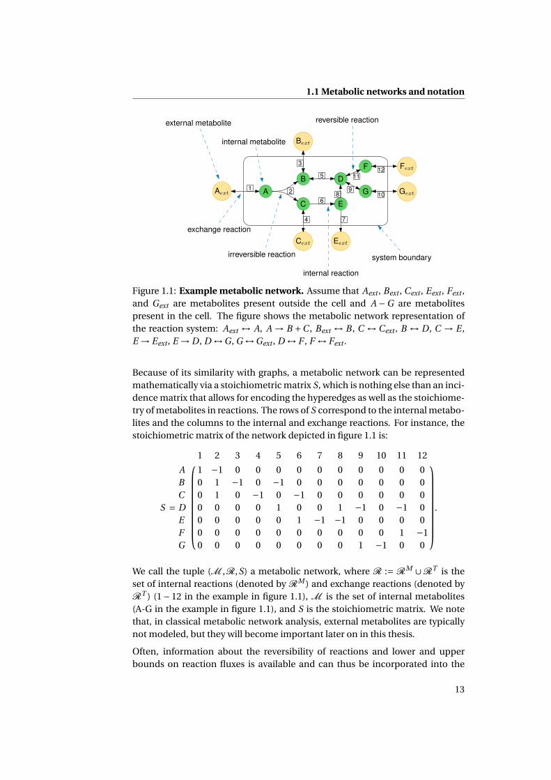
Figure 1.1: Example metabolic network. Assume that Aext , Bext , Cext , Eext , Fext ,and Gext are metabolites present outside the cell and A −G are metabolitespresent in the cell. The figure shows the metabolic network representation ofthe reaction system: Aext ↔ A, A → B +C , Bext ↔ B , C ↔ Cext , B ↔ D , C → E ,E → Eext , E → D , D ↔G , G ↔Gext , D ↔ F , F ↔ Fext .
Because of its similarity with graphs, a metabolic network can be representedmathematically via a stoichiometric matrix S, which is nothing else than an inci-dence matrix that allows for encoding the hyperedges as well as the stoichiome-try of metabolites in reactions. The rows of S correspond to the internal metabo-lites and the columns to the internal and exchange reactions. For instance, thestoichiometric matrix of the network depicted in figure 1.1 is:
S =
1 2 3 4 5 6 7 8 9 10 11 12
A 1 −1 0 0 0 0 0 0 0 0 0 0B 0 1 −1 0 −1 0 0 0 0 0 0 0C 0 1 0 −1 0 −1 0 0 0 0 0 0D 0 0 0 0 1 0 0 1 −1 0 −1 0E 0 0 0 0 0 1 −1 −1 0 0 0 0F 0 0 0 0 0 0 0 0 0 0 1 −1G 0 0 0 0 0 0 0 0 1 −1 0 0
.
We call the tuple (M ,R,S) a metabolic network, where R := RM ∪RT is theset of internal reactions (denoted by RM ) and exchange reactions (denoted byRT ) (1− 12 in the example in figure 1.1), M is the set of internal metabolites(A-G in the example in figure 1.1), and S is the stoichiometric matrix. We notethat, in classical metabolic network analysis, external metabolites are typicallynot modeled, but they will become important later on in this thesis.
Often, information about the reversibility of reactions and lower and upperbounds on reaction fluxes is available and can thus be incorporated into the
13

Chapter 1. Introduction
mathematical description. We denote by Irr ⊆R the set of irreversible reactions,by l,u ∈RR the lower and upper reaction rate (flux) bounds.
We use S∗r to denote the column corresponding to reaction r and Sm∗ to de-note the row corresponding to metabolite m respectively. Smr then denotes thestoichiometric coefficient of metabolite m in reaction r . We will use sets of in-dices to denote submatrices: S∗Irr for example will denote the submatrix of Scorresponding to all irreversible reactions Irr.
Of particular importance for the metabolic modeling is also the set of enzymesthat catalyze the reactions, which we denote as E . We use v = (
v1, . . . ,v|R|)ᵀ to de-
note the fluxes (the rates at which substrates are converted into products, alsoknown as reaction rates), c = (
c1, . . . ,c|M |)ᵀ to denote metabolite concentrations,
e = (e1, . . . ,e|E |
)ᵀ to denote the set of enzyme concentrations, where xᵀ denotesthe transpose of the vector x. We useµ to denote the growth rate of the organism.Since some of the methods we will use involve molar amounts rather than con-centrations, we use ni to denote the molar amount of compound i , irrespectiveof whether it is a metabolite or an enzyme.
Please note that the fluxes v, the concentrations c,e, the molar amounts n, andthe growth rate µ can in some cases depend on time. Furthermore, v(t ) ∈ R|R|,c(t ) ∈ R|M |
≥0 , e(t ) ∈ R|E |≥0 , and n ∈ R|M∪E |
≥0 are vectors and thus written in boldface,as all other vectors appearing in this thesis. Equality or inequality relationshipsbetween vectors and constants apply elementwise, i.e., a ≥ 0 indicates that everyentry in the vector a is greater or equal to zero.
1.2 Metabolic modeling
1.2.1 Dynamic modeling
A classical and well-known way of modeling biochemical reaction systems is viasystems of ordinary differential equations that describe the rate of change ofmetabolite concentrations c (Klipp et al., 2008). Assuming a constant cell vol-ume, the rate of change of the concentration ci of a metabolite i is given by thedifference between its rate of production and the rate at which it is consumed:
dci (t )
d t= vproduction −vconsumption.
This can be written for metabolic networks using the stoichiometric matrix S:
dc(t )
d t= Sv(t ).
14

1.2 Metabolic modeling
The reaction rates v are usually nonlinear functions of the substrate and enzymeconcentrations1 and we can write them as:
v(t ) = f (e(t ),c(t )).
The deterministic kinetic rate laws f : R|E |≥0 ×R|M |
≥0 → R|R| are largely unknown,and even if they are known, they depend on kinetic parameters that need tobe determined experimentally. For example, if we assume Michaelis-Mentenkinetics (Michaelis and Menten, 1913) for a simple irreversible reaction j : A →B , the rate law is given by
v j = e j kcatcA
cA +KM, (MM)
where KM is the so-called Michaelis constant, which is a constant specific toeach reaction, and kcat is the turnover rate of the respective enzyme and is de-fined as the maximum number of molecules of substrate that the enzyme canconvert to product per catalytic site per unit of time.
To the basic kinetic model presented above, various degrees of regulatory infor-mation can be added, including but not limited to enzyme production dynamicsvia the ribosomes depending on transcription factor activities or various typesof enzyme activity inhibition.
At genome-scale, such modeling approaches are largely limited by the hugenumber of reactions, the nonlinearity of the kinetic rate laws and the missinginformation about kinetic parameters. Moreover, the number of enzymologicalstudies has reduced significantly since 1998 (based on statistics on entries inthe BRENDA database (Schomburg et al., 2013)), and there is little hope thatthis situation will become better in the near future (Holzhütter, 2004).
1.2.2 Constraint-based modeling
To overcome the computational limitations and data requirements of kineticmodeling of reaction networks, constraint-based modeling has emerged as yetanother popular approach (Price et al., 2004; Bordbar et al., 2014). One of thecore assumptions of this type of modeling is that the internal metabolites areat steady-state, i.e., their production and consumption fluxes are balanced andthus their level is assumed to be constant.
This steady-state assumption can be motivated from two different perspectives.In the time-scales perspective, we use the fact that metabolism is much fasterthan other cellular processes such as gene expression. Hence, the steady-stateassumption is derived as a quasi-steady-state approximation of the metabolism
1There are other additional factors that can influence the reaction rate such as (allosteric) en-zyme inhibitors, pH or temperature. Depending on the level of detail of the model, these can alsobe included or left out.
15

Chapter 1. Introduction
that adapts to the changing cellular conditions. However, the time scale separa-tion argument is not necessarily needed to derive the steady-state assumption.A second perspective, on which we will focus in chapter 3, states that, on the longrun, no metabolite can accumulate or deplete. In contrast to the first perspec-tive it is not immediately clear how this perspective can be captured mathemat-ically and what assumptions are required to obtain the steady-state condition.We leave the answers to this question for chapter 3, and now focus on what arethe consequences of assuming intracellular metabolites to be at steady-state.
This assumption essentially eliminates the need for kinetic rate laws and param-eters. It can be written as:
Sv = 0.
We will see in chapter 3 that one way to understand v is as an average over timeof v(t ).
This transforms the problem into a linear equation system which is much easierto analyze. It however comes at several expenses: the solution space of this sys-tem, even after adding constraints about reaction directionality and bounds, isa polyhedron and hence the system is underdetermined. Additionally, a hiddenassumption comes into place, namely that all enzymes are present and in thecorrect concentrations to sustain the resulting fluxes.
Additional information about the reversibility of reactions, inferred, for exam-ple, from thermodynamic considerations, can be incorporated by adding theconstraint vIrr ≥ 0.
To limit the size of the system, assumptions about the cellular behavior aremade. Namely, the cell is assumed to optimize a particular biological objec-tive. In the first article to introduce constraint-based modeling for metabolicnetworks, the assumption was that the cell tends to optimize its growth rate inthe form of biomass production (“It is expected that the metabolic phenotypeof wild type strains is defined by a tendency to optimize their growth rates, atleast in nutritionally rich environments such as those found in the majority ofbioprocesses.”, Varma and Palsson (1994), p. 995).
The maximization of biomass production is usually done by adding a pseudore-action to the stoichiometric matrix that consumes all metabolites (amino acids,fatty acids, carbohydrates, ATP, cofactors etc.) assumed to be needed for cellulargrowth, and flux through this reaction is maximized. This approach is known asflux balance analysis (Varma and Palsson, 1994; Orth et al., 2010), in short FBA,and is shown below:
maxv∈R|R|
vbiomass
s.t. Sv = 0
vIrr ≥ 0
l ≤ v ≤ u,
16

1.2 Metabolic modeling
where l,u are lower and upper bounds on the reaction fluxes that may come ei-ther from information about maximal reaction rates or as a need to limit growthyield as explained below.
Later on, a series of other objectives have been introduced. For an evaluationof objective functions for predicting intracellular fluxes in the bacterium Es-cherichia coli we refer the reader to (Schuetz et al., 2007). It turns out that notonly there is no universally assumed cellular objective, but some of them mayeven be conflicting. Take, for instance, the fact that the cell is assumed to turnoff “jobless” pathways to save on enzyme costs, but, at the same time, it is alsoassumed to be minimizing response time to changes in the environment, i.e.,have the enzymes already produced to be able to react immediately. This is howmultiobjective modeling of metabolism came to life (Schuetz et al., 2012).
When dealing with multiobjective problems, we no longer talk about unique op-timal objective values and unique growth yields, but about sets of optimal solu-tions known as the Pareto front. This is the set of solutions that cannot be im-proved with respect to one objective without making another objective worse.All these solutions are optimal with respect to the given objectives, but they rep-resent different compromises between the individual objectives. In addition,multiobjective problems should not be confused with problems that consider asingle objective function with multiple weighted terms. In the latter case, onlyone of the Pareto solutions is found instead of the Pareto front, and this solu-tion may be very sensitive to the weighting of the individual objective terms.Indeed, it has been shown via a combination of experimental and computa-tional methods that, for the bacterium E. coli, the metabolism works close to thePareto-optimal surface defined by competing objectives (Schuetz et al., 2012).In this case, the Pareto front is determined by three objectives: maximization ofbiomass yield, maximization of ATP yield and minimization of total flux throughthe network.
The advantage of the constraint-based formulation is that it gives rise to a linearoptimization problem, also known as linear program (LP), which can be solvedvery fast. Since unlimited nutrient uptake would give rise to unlimited growth,usually a constraint that limits nutrient uptake is added, such as vglucose uptake ≤1, meaning that the cell is only allowed to take up one unit of e.g. glucose perunit time, i.e., the flux through the glucose uptake reaction is at most one.
By introducing the limits on nutrient uptake however, we do not optimizegrowth rate anymore, but growth yield. That is, FBA does not actually predicthow fast the organism can grow, but how efficiently it can turn the nutrient intogrowth. This is however not what microorganisms living in rich environmentsdo. Rather, at high substrate concentration the organisms opt for maximizinggrowth rate and, in doing this, they sometimes choose yield-suboptimalstrategies. Only when the substrate becomes limiting do microorganisms useyield-optimal strategies (Molenaar et al., 2009).
17

Chapter 1. Introduction
To give some examples, yeast cells use fermentation even in the presence of oxy-gen to process glucose at high extracellular glucose concentrations (van Dijkenet al., 1993). However, fermentation is yield-suboptimal since it produces a totalof only two ATP molecules per molecule of glucose. The yield-optimal strategywould be to use respiration, which results, depending on the organism, in about30 molecules of ATP per glucose molecule.
On the other hand, although it has a high ATP yield, aerobic conversion of glu-cose employs large pathways with many enzymes. To run all these pathwaysat a high rate, the cell has to make the effort of producing all the necessary en-zymes. In addition, the production of all these enzymes in high amounts resultsin molecular crowding of the cell, which can impede other cellular processes byhindering diffusion.
For a comparison, in fermentation, the whole Krebs cycle and oxidative phos-phorylation are replaced by only three reactions needing three enzymes forcatalysis.
Not only yeast, but many other biological systems are known for not actingyield-optimally. Other examples are cancer cells that display the Warburg effect(Warburg, 1956), or the lactic acid fermentation of Bacillus subtilis (Sonenshein,2007). These examples, together with additional theoretical and experimentalobservations (Schuster et al., 2008), point out that using growth yield as a cuefor growth rate may lead to false predictions. Thus, FBA is not always the way togo for predicting metabolic flux.
Another important point is that maximization of yield comes together witha hidden assumption: enzymes are present in the correct concentrations forachieving optimal yield reaction rates. However, in reality, before using anenzyme, the organism has to produce it. Producing enzymes in very highconcentrations comes at two expenses: cellular resources have to be investedin enzymes, and increased molecular crowding that can hinder other biologicalprocesses.
While modeling the former is the very topic of this thesis and will be discussedextensively by giving a state of the art of metabolic resource allocation in chap-ter 2, the latter we briefly explain here.
The main idea of accounting for molecular crowding as a way to limit reactionflux has been addressed in (Beg et al., 2007) and in (Shlomi et al., 2011) via im-posing extra constraints on the solution space. The constraints can be formu-lated either on the total enzyme mass, as done in (Shlomi et al., 2011), or on thetotal enzyme volume, as done in (Beg et al., 2007), following roughly the sameprinciples. One typically imposes a constraint that limits the total sum of fluxes,weighted by the mass or the volume of respective metabolic enzymes. To imposethese constraints one typically needs additional data such as enzyme molecularweights or volumes, which may not always be available in the literature.
18

1.3 Cellular resource allocation
In addition to the FBA disadvantages already explained, we note that it is rarelythe case that FBA reports a unique optimal flux distribution. More often, thereare several flux vectors with the same optimal growth yield. While imposingthermodynamic constraints can help to further shrink the optimal solutionspace (Beard et al., 2002, 2004; Schellenberger et al., 2011; Hamilton et al., 2013;Reimers, 2014) by further constraining some reaction reversibilities, it is rarelythe case that this results in a unique solution. For this reason, typically addi-tional methods like flux variability analysis (Mahadevan and Schilling, 2003)need to be used to check the optimal solution variability, and flux modules(Kelk et al., 2012; Müller and Bockmayr, 2014; Reimers et al., 2015) can be usedto visualize which alternate pathways give rise to the variability.
1.3 Cellular resource allocationAnother view in metabolic modeling is that microorganisms are autocatalyticsystems. They invest resources in terms of nutrients and time into enzymes thatthey then use to catalyze reactions to again produce more enzymes. In addi-tion, ribosomes need to be present to translate the enzymes, and the ribosomesthemselves need to be produced, following the same principle. A question ofprioritization then arises: in which components should the cell invest such thatit grows optimally?
This is why, in recent years, the systems biology of metabolism has moved moreand more from classical metabolic network study towards the study of growthas a result of an optimized cellular economy.
The ideas that a cell minimizes the total enzyme concentration needed for afixed steady-state flux and that there exists a competition among reactions foravailable enzyme resources are however not new, but go back to (Brown, 1991)and (Klipp and Heinrich, 1999). Moreover, similar ideas have been used to studyactivation of metabolic pathways and enzyme allocation under a constraint oflimited total enzymatic capacity starting with (Klipp et al., 2002). This was thenfurther investigated using experimental (Zaslaver et al., 2004) as well as mathe-matical techniques (Oyarzún et al., 2009; Bartl et al., 2010) and was even broughtforward in a multiobjective dynamic optimization study (de Hijas-Liste et al.,2014).
In their article, (Molenaar et al., 2009) pointed out that the limited totalproteome constraint does not apply only to metabolism, but to all cellular sub-systems, which have to share resources among each other. In this study a smalldynamic model of a self-replicating system is used to explain how overflowmetabolism arises by means of tradeoffs between different growth strategies.Further on, Goelzer et al. (2011) introduced resource balance analysis (RBA), asa means of predicting the cell composition of bacteria in a specific (constant)environment through a convex optimization problem that takes into accountthe bioenergetic costs of running a pathway. More or less in parallel, Lerman
19
Chapter 1. Introduction
et al. (2012) introduced the idea of an integrated model of metabolism andgene expression (ME model) as a means to explore the relationship betweengenotype and phenotype using biochemical representations of transcriptionand translation processes. Their research group then continued with an MEmodel of the model organism Escherichia coli (O’Brien et al., 2013). Alsoexperimental studies focused on relating absolute protein abundances to howmetabolic pathways balance production costs and activity requirements (Liet al., 2014).
These steady-state resource allocation formalisms have then been combinedwith the dynamic optimization ideas in (Klipp et al., 2002; Oyarzún et al., 2009;de Hijas-Liste et al., 2014), to understand how resources are distributed in a dy-namically changing environment by means of a dynamic enzyme-cost flux bal-ance analysis (deFBA) and conditional flux balance analysis (cFBA) (Waldherret al., 2015; Rügen et al., 2015).
Such dynamic resource allocation models have a wide area of applicability. Onesuch an example is the study of microorganisms growing in industry-scale biore-actors. There, the organism has to balance resources not only in order to be ableto grow optimally, but also in order to survive transitions through local hetero-geneities of the reactor. The ability to take such transitions into account withinmetabolism has been shown to be crucial for survival (van Heerden et al., 2014).
In addition, a perfect study case is the metabolism of phototrophic organisms,who live in regular day-night light conditions. Dynamic resource allocationmodeling helps us understand how they organize their synthesis and storageprocesses following light availability.
The main underlying hypothesis of such studies is that organisms have beenshaped through evolution by reoccurring changes in their environment and thatthe observed patterns in their metabolism are the result of optimized growthin this changing environment. Thus, along the lines of (Klipp, 2009), we cancheck using optimization principles and models if what we observe in natureare indeed optimal behaviors.
1.4 Structure of this thesisFollowing the recent developments in optimal dynamic resource allocation for-malisms, this thesis focuses on modeling and understanding resource allocationin large (sometimes genome-scale) metabolic models.
In chapter 2 we start with a state of the art overview on metabolic resource allo-cation formalisms.
We then present in chapter 3 a new mathematical derivation of the widely usedsteady-state assumption that motivates its successful use in many applications.This derivation can then be used to quickly provide upper bounds on growthrates in dynamic resource allocation problems.
20

1.4 Structure of this thesis
Chapter 4 then provides a protocol on how to generate a dynamic resource allo-cation model. Before we turn our attention to applications, we present in chap-ter 5 some guidelines, useful problem transformations and instructions for nu-merically solving the resulting dynamic resource allocation problems.
Having set the stage this way, we proceed in chapter 6 with an in depth study atgenome-scale of the metabolic resource allocation in the cyanobacterium Syne-chococcus elongatus PCC 7942. This is the first genome-scale dynamic resourceallocation study and it presents insight into the temporal organization of synthe-sis processes following light availability. Moreover, it shows that the linear pat-tern of the accumulation of storage (glycogen) throughout the day period is anoptimal behavior that arises as a tradeoff between several conflicting resourceallocation objectives.
We continue in chapter 7 with a study of yeast living in dynamically changingenvironments. This is motivated by the observation that, in industrial-scalebioreactors, yeast cells live in a changing environment governed by local het-erogeneities. We therefore want to understand what mechanisms enable someof the cells to survive such environment transitions, and why other subpopu-lations do not make it through the transitions and die out. We show that over-flow metabolism and diauxie, phenomenons that are not exclusively observedin yeast but widely spread in nature, are optimal behaviors from a resource allo-cation perspective. Moreover, we investigate how one can use resource alloca-tion models to understand how yeast adapts to oxygen and nutrient availabilityshifts.
A next step, which we explore in chapter 8, is the perspective of using timecourses from dynamic resource allocation models to infer the regulatory struc-tures that implement these optimal behaviors.
We conclude by summarizing the results of the thesis and listing possible nextsteps in using dynamic resource allocation models to understand metabolismand its regulation.
21


Chapter 2
Resource allocation formalisms
This chapter aims at giving an overview of the current metabolic resource allo-cation formalisms and exemplifies them using the toy model proposed in (Mole-naar et al., 2009). This will help us better understand the methods used for thecase studies in chapters 6 and 7.
2.1 Resource allocation principles in a self-replicator
In their article, (Molenaar et al., 2009) start by noting that there are several com-mon patterns that can be observed in the physiology of unicellular organisms,such as increase of cell size and ribosomal content with increasing growth rate,or a shift to energetically inefficient metabolism at high growth rates. Moreover,such patterns are not only observed in unicellular organisms, but also in tumorcells for example. They argue that such patterns hint at the existence of designprinciples that result in the optimization of evolutionary fitness.
This idea of fitness optimality is not new. It has already been applied successfullyin the study of cellular subsystems like metabolism. There, global metabolic re-action rates (fluxes) are predicted using a network of biochemical reactions andassuming that cells have evolved towards optimizing growth yield in a constantenvironment. While the resulting predictions have been shown to fit experimen-tal measurements relatively well (Edwards et al., 2001; Ibarra et al., 2002), suchmodels fail to predict the usage of inefficient metabolic routes and “spilling” ofresources at high nutrient concentrations, a phenomenon known in the litera-ture as overflow metabolism. The reason, according to (Molenaar et al., 2009),lies in the modeling of only one subsystem (metabolism), rather than the sub-system in its context, where the cell would have to produce catalytic units be-fore these can be used to catalyze reactions and would have to balance the costsand benefits of the macromolecules it produces together with the effects of suchmacromolecules on the overall growth rate.
23

Chapter 2. Resource allocation formalisms
To prove their theory, (Molenaar et al., 2009) propose a self-replicator model thatcontains most cellular subsystems, including production of macromoleculessuch as membrane, the ribosome, or transporters. We have reproduced thisself-replicator model in figure 2.1, and we will use it to explain the state ofthe art of resource allocation formalisms in the next sections. In addition, wepresent in table 2.1 the list of species and reactions of this model.
Q
R
P
M
Nin
T
Nout
L
Figure 2.1: Self-replicator toy model proposed by (Molenaar et al., 2009) in theirresource allocation study. Extracellular nutrients are depicted in yellow, intra-cellular metabolites are shown in green, and macromolecules in blue. Reactionsare shown in continuous arrows, while catalysis relationships are in dashed ar-rows. The model contains all subsystems of a cell: Nout , extracellular nutrientsource; Nin, intracellular nutrient; P, metabolic precursors; L, lipid synthesis en-zyme; M, metabolic enzyme; Q, lipid membrane; R, ribosome; T, transporter.
(Molenaar et al., 2009) consider the self-replicator system in a growth mediumwith infinite volume and a constant substrate concentration cNout . Furthermore,they assume the main objective of the system is to maximize the growth rate µunder a balanced growth condition, where each component grows at the samerate. The main limitations of growth are constraints imposed by physics andchemistry that we will detail in the following subsections.
2.1.1 Growth rate and dilution
To understand the growth rate µ, we need to look at the volume of the system,which is assumed to grow exponentially, following the equation
V (t ) =V0 ·eµ·t , (2.1)
24

2.1 Resource allocation principles in a self-replicator
Table 2.1: List of species, reactions, and catalysis relationships for the model infigure 2.1. We note that we have a one to one correspondence between reactionsand their catalyzing enzymes and we therefore denote them by the same letter.
External metabolites: Nout
Internal metabolites: M = {Nin, P, Q}Enzymes: E = {L, M, R, T}
Reactions Catalyzed by Turnover rateNout → Nin T 7Nin → P M 5P → Q L 5P → L R 3P → M R 3P → R R 3P → T R 3
where V0 is the initial volume of the bacterial population. By taking the deriva-tive in equation 2.1, we obtain
µ= 1
V (t )
dV (t )
d t, (2.2)
consistent with the definition in (Heinrich and Schuster, 1996). The case wherethe growth rate is not constant is discussed in section 5.3.
Following the definition of concentration of a molecule i as number of molesni (t ) per volume V (t ), ci (t ) = ni (t )
V (t ) , we obtain then that
d
d tci (t ) = d
d t
ni (t )
V (t )
= dni (t )
d t
1
V (t )− dV (t )
d t
1
V (t )
ni (t )
V (t )
= dni (t )
d t
1
V (t )︸ ︷︷ ︸production
− µni (t )
V (t ).︸ ︷︷ ︸
dilution by growth
2.1.2 Mass balance equations
The authors of (Molenaar et al., 2009) assume an exponential growth model forthe biomass of the system where µ is the constant specific growth rate. In addi-tion, they assume a steady-state in the form of balanced growth, i.e., the rates ofproduction and dilution by growth of each intracellular species are balanced as
0 = dc(t )
d t=∑
vsynthesis(t )−∑vdilution(t ) = SM∗v(t )−µc(t ),
0 = de(t )
d t=∑
vsynthesis(t )−∑vdilution(t ) = SE∗v(t )−µe(t ),
25

Chapter 2. Resource allocation formalisms
where S is the stoichiometric matrix. Therefore, they assume that the fluxes andthe concentrations are constant and thus we omit their time dependency in thissection and write simply v, c, and e.
The system can modulate the growth rate µ, by modulating the production rateof each protein. That means that the fractions of ribosomes used for the synthe-sis of each protein can be changed and for each i ∈ {L, M , R, T } we have
dei (t )
d t= Si ∗v(t )−µei (t ) =αi vR −µei = 0,
where vR is the rate at which the total ribosome pool synthesizes proteins, αi
is the fraction of this pool dedicated to the synthesis of protein i , and the stoi-chiometry Si ∗ is omitted because all coefficients are one.
2.1.3 Kinetics of rate equations
We have already seen in the previous section that the flux values v play an im-portant role in the growth of the system. In this model, they are all assumed tofollow irreversible Michaelis-Menten kinetics, as described in table 2.2.
Table 2.2: Rate equations for the reactions of the self-replicator. k icat is the
turnover rate of enzyme i , which can be found in table 2.1. KM is the Michaelisconstant and is assumed to be equal to 1 for all reactions.
Reaction Rate equation
Nout → Nin vT = kTcat ·eT ·cNout
KM +cNout
Nin → P vM = kMcat ·eM ·cNin
KM +cNin
P → Q vL = kLcat ·eL ·cP
KM +cP
P → i ∈ {L, M , R, T } vR = kRcat ·eR ·cP
KM +cP
2.1.4 Membrane integrity
An important observation is that the lipids Q, which we call from now on quotametabolites, will in fact never be produced in a solution that is optimal withrespect to maximizing µ given the constraints above. They are simply a drainof resources that does not contribute to the autocatalytic nature of the system.However, in reality, the membrane lipids play an important role in keeping theintegrity of a cell. Therefore, a constraint is imposed to make sure that the mem-brane of the self-replicator is not only made of transporters, but a lipid quota is
26

2.1 Resource allocation principles in a self-replicator
also present. This is done by imposing that the amount of transporters needs tobe at most equal to that of membrane lipids, i.e.,
cQ ≥ eT .
Just as the lipids, also DNA and RNA are important components without cat-alytic role that are essential for replicating the cell. They are not considered ex-plicitly in this model, but they will later on play a role in metabolism and expres-sion models (ME models), resource balance analysis (RBA), dynamic enzyme-cost flux balance analysis (deFBA), and conditional flux balance analysis (cFBA),which we explain in later chapters. We call these quota metabolites, to highlightthat a certain quota in the total biomass has to be dedicated to them.
2.1.5 Total proteome is limited
The volume of a cell is obviously not infinite, and that means there is also a limitto how much protein can be contained inside a cell. Therefore, the authors of(Molenaar et al., 2009) impose a constraint on the total amount of proteins as
∑i∈{L, M , R, T }
ei ≤ 1.
As mentioned in the introduction, the idea of such a constraint is not new. Aversion of this constraint has been already introduced in (Klipp et al., 2002) andlater on used in flux balance analysis with molecular crowding (Beg et al., 2007),as well as in other metabolic resource allocation formalisms as detailed in thefollowing sections.
2.1.6 Additional constraints
There are also more obvious constraints that we need for the self-replicatormodel. For instance, species concentrations should be nonnegative, which canbe expressed as
c,e ≥ 0.
Additional volume constraints are used in the article. We do not detail them be-cause they do not bring any additional understanding of the resource allocation.
Finally, the ribosome fractions used for protein synthesis should sum up to 1,
∑i∈{L, M , R, T }
αi = 1.
27

Chapter 2. Resource allocation formalisms
2.1.7 The nonlinear optimization problem
Putting together the constraints above, we obtain a nonlinear optimizationproblem (NLP) over the variables µ, c, e, v, α for every fixed cNout :
maxα,µ,c,e,v
µ
s.t. Si∗ ·v−µ ·ci = 0 ∀i ∈ {Nin,P,Q} (2.3)
αi ·vR −µ ·ei = 0 ∀i ∈ {L, M , R, T } (2.4)
vT = kTcat ·eT ·cNout
KM +cNout
(2.5)
vM = kMcat ·eM ·cNin
KM +cNin
(2.6)
vi =k i
cat ·ei ·cP
KM +cP∀i ∈ {L,R} (2.7)
cQ ≥ eT (2.8)∑i∈{L, M , R, T }
ei ≤ 1 (2.9)
α,c,e ≥ 0 (2.10)∑i∈{L, M , R, T }
αi = 1. (2.11)
The authors solve the optimization problem using GAMS (https://www.gams.com/) in combination with the KNITRO solver. This solver only guarantees find-ing local solutions to the NLP. The authors then check the global solution op-timality using the LINDOGlobal solver. Such solvers can use branch and cutmethods to break the NLP into subproblems which are either infeasible, optimalor that are in turn split again. At additional computational cost, they can auto-matically linearize some of the nonlinear relationships. They guarantee globaloptimality within a user-set tolerance. Please note that using an NLP solver forsuch a small model may be feasible in terms of the solving time, but it will defi-nitely not be an option anymore if the problem grows to hundreds or even thou-sands of variables.
2.1.8 Results and extensions
Although it is a simple model, the self-replicator and its extensions presented in(Molenaar et al., 2009) are capable of displaying many behaviors observed in realorganisms. The authors show how growth of the ribosome pool with increasinggrowth rate, overflow metabolism, or growth strategies on two substrates ariseas tradeoffs between the costs and benefits of proteome allocation.
The model has inspired a series of resource allocation studies, of which we detailresource balance analysis (RBA), metabolism and gene expression models (ME
28

2.2 Resource balance analysis
models), dynamic enzyme-cost flux balance analysis (deFBA), and conditionalflux balance analysis (cFBA) in the following sections.
2.2 Resource balance analysisIntroduced by (Goelzer et al., 2011), RBA exploits the same idea as the resourceallocation model in (Molenaar et al., 2009): modeling the cell as an interdepen-dence of several subsystems that complete different tasks contributing to growthand that share common resources. There are however several differences to thework of (Goelzer et al., 2011), which we will detail below.
To begin with, the authors of RBA give a formal definition of the growth rateµ as a function of the volume of the cell, as we have already detailed it in theprevious section. As in our steady-state assumption including dilution effectsin section 5.3 and as in the article of (Molenaar et al., 2009), they note that atsteady-state the production and dilution of all cellular macromolecules shouldbalance in order to maintain their concentrations constant. Furthermore, theyalso assume that the fluxes are constant.
2.2.1 Relaxing steady-state constraints and imposing quota
However, they relax the steady-state constraint compared to equations (2.3) and(2.4), and allow overproduction of metabolic precursors and macromolecules,but not of metabolic intermediates. Assuming the stoichiometric matrix alsocontains the macromolecule production reactions, equations (2.3) and (2.4) arereplaced by
SP∗ ·v ≥ 0,
SNin∗ ·v = 0,
Si∗ ·v−µ ·ei ≥ 0, ∀i ∈ {L, M ,R,T },
SQ∗ ·v−µ ·cQ ≥ 0.
We note also that only dilution of macromolecules by cell growth is modeled inRBA, but not dilution of internal metabolites Nin and P . In chapter 5 we estimatethe error that we make by neglecting metabolite dilution via cell growth.
Furthermore, by including Q in the latter equation and fixing the requiredamount cQ ≥ 0, quota metabolites are required to also grow at the rate µ.
2.2.2 Kinetics of rate equations are replaced by linear constraints
Reaction rates in RBA are not modeled using kinetic rate laws as in (Molenaaret al., 2009). Instead the authors assume that enzymes are substrate-saturatedand that the reaction rate is given by the product of the turnover rate and theenzyme amount. As reasoning, the authors cite a PhD thesis written in French
29

Chapter 2. Resource allocation formalisms
that is not available online, but which suggests that “at steady state, the enzymesoperate at (or close to) saturation”(Goelzer et al., 2011). Although not mentionedin the RBA article, in (Bennett et al., 2009) absolute metabolite concentrationsin Escherichia coli are compared to the KM values of their degrading enzymes,and the results indeed indicate that most enzymes analyzed (83%) are more than50% saturated with substrate. Moreover, 59% of the analyzed enzymes processsubstrates in a concentration that is more than 10−fold higher than their KM .These results indicate that, for most reactions r catalyzed by an enzyme E , thereaction flux is somewhere in the interval [ 1
2 kEcat ·eE , kE
cat ·eE ], assuming simpleMichaelis-Menten kinetics. The equality assumption that vr = kE
cat · eE in RBAis still quite strong, since it forces flux whenever the enzyme is present althoughregulatory effects may impose that only a fraction of this flux is present at times.
Nevertheless, this assumption simplifies the equations for fluxes (2.5)-(2.7) to
|vi | = k icat ·ei , ∀i ∈ {T, M ,L,R}.
This is the first time such an approximation is introduced in order to linearizekinetic expressions. The absolute value is present because some reactions maybe reversible, and in that case their flux values, albeit negative, should still beconstrained by the enzyme amount. This usage of the absolute value in the con-straint introduces a nonlinearity into the optimization problem. However, thisis easily resolved by introducing extra variables vmax ≥ 0, and requiring that
vi −vmaxi ≤ 0 and −vi −vmax
i ≤ 0, ∀i ∈ {T, M ,L,R}.
Note that this transformation relaxes the original equality constraint, into vr ≤kE
cat ·eE , and thus the saturation hypothesis is given up.
It should additionally be noted that, instead of using the fractions α to modelcompetition of the protein synthesis reactions for the ribosome, RBA uses anupper bound on the sum of enzyme production fluxes in combination with therate equation linearization as ∑
i∈{T,M ,L,R}vRi ≤ kR
cat ·eR ,
where vRi denotes the synthesis flux for protein i .
2.2.3 Modeling volume vs. modeling density
As in (Molenaar et al., 2009), RBA also does not explicitly model volume. In-stead, a density constraint is used that requires the intracellular density to re-main constant to ensure diffusion is not impaired. In detail, the weighted sumof the densities of the macromolecules is bounded by the mean density D of thecell as ∑
i∈{T,L,M ,R}ρi ·ei +ρQ ·cQ ≤ D ,
30

2.2 Resource balance analysis
where ρi is the density of macromolecule i . This effectively means that the sat-uration assumption from above is given up.
This constraint is only imposed for the macromolecules, since metabolite con-centrations are not modeled explicitly and metabolites are assumed to be smallenough to not impair diffusion. The main role of this constraint is to provide anupper bound on total proteome, similar to constraint (2.9).
2.2.4 Nutrient uptake
The RBA article does not explicitly mention how extracellular nutrient uptake ismodeled. We assume that they use a Michaelis-Menten rate law as in (Molenaaret al., 2009), and fix the parameters kT
cat ,KM , as well as the substrate concentra-tion cNout . If this is the case, the uptake rate vT depends linearly on the amountof enzyme eT , while the rest of the terms are fixed, as
vT = kTcat ·eT ·cNout
KM +cNout
.
2.2.5 The quadratically constrained optimization problem
By replacing the kinetic expressions for the fluxes with linear terms that onlydepend on enzyme concentrations and kcat , RBA casts the resource allocationproblem into a quadratic program, with µ as common variable in all quadraticterms. Putting together all constraints, RBA for the toy model in figure 2.1 isgiven by:
maxµ,c,e,v,vmax
µ
s.t. SP∗ ·v ≥ 0 (2.12)
SNin∗ ·v = 0 (2.13)
Si∗ ·v−µ ·ei ≥ 0 ∀i ∈ {L, M ,R,T } (2.14)
SQ∗ ·v−µ ·cQ ≥ 0 (2.15)
vmaxi = k i
cat ·ei ∀i ∈ {L, M ,R,T } (2.16)
vi −vmaxi ≤ 0 ∀i ∈ {L, M ,R,T } (2.17)
−vi −vmaxi ≤ 0 ∀i ∈ {L, M ,R,T } (2.18)∑
i∈{T,M ,L,R}vRi ≤ kR
cat ·eR (2.19)
vT = kTcat ·eT ·cNout
KM +cNout
(2.20)∑i∈{T,L,M ,R}
ρi ·ei +ρQ ·cQ ≤ D (2.21)
vmax ,c,e,µ≥ 0. (2.22)
31
Chapter 2. Resource allocation formalisms
Sinceµ is common to all quadratic terms, instead of solving a quadratic problemone can use a half-interval search (also known as binary search) over µ, and forevery fixed µ solve a linear feasibility problem. Briefly, one starts with a verysmall fixed value of µ and successively doubles it until the resulting feasibilityproblem becomes infeasible. Once this is the case, a typical binary search can beused to search the optimal value for µ, which is now in the interval between thelast feasible µ and its double. Usually one has to set a tolerance for the smallestchange in µ at which this procedure should stop.
2.2.6 Mathematical and biological implications
In addition to providing a resource allocation framework that is efficiently solv-able also for large-scale systems, the authors prove mathematically several im-portant properties about the framework, of which we mention here a few.
The article provides a proof that, if the resulting feasibility problem is feasible fora fixed µ∗, then it is also feasible for any other value of µ in the interval [0,µ∗].They also prove that there exists a finite optimal µ∗ and that every value largerthan this will result in an infeasible problem.
The authors show that the growth rate µ increases when the fixed required non-catalytic biomass quota cQ is decreased. This fact has also been proven experi-mentally in (Fischer and Sauer, 2005) by deleting the inductor of expression forflagellar proteins in Bacillus subtilis, which are proteins only required for mobil-ity, with no catalytic role. The resulting mutant strain displayed a faster growthrate than the wild type.
Last but not least, (Goelzer et al., 2011) show that increasing the turnover ratesreduces the necessary amounts of enzymes for running the same flux and thusincreases growth rate, and that “cheap” pathways (in terms of synthesis invest-ment) are nearly always preferred (e.g. uptake amino acids rather than de novosynthesis). They also point out that an “expensive” pathway may be preferredsometimes if it reduces cost of producing a co-metabolite needed somewhereelse in the system.
(Goelzer et al., 2011) apply RBA to a model of Bacillus subtilis metabolism, with342 genes, 277 enzymes, 54 transporters, and 358 metabolic reactions and showthat the modular configuration of this metabolic network is a function of themedium composition.
2.2.7 Extension through metabolism and gene expression models
Up to now we have seen how RBA takes into account resource investment intometabolic pathways by modeling protein translation explicitly. One can how-ever go one level of detail higher, as in metabolism and gene expression models(ME models) (Lerman et al., 2012; O’Brien et al., 2013), and also model the tran-scription process. One can then provide limits on the number of proteins that
32

2.2 Resource balance analysis
can be translated from a given messenger RNA (mRNA) before this mRNA is de-graded or passed on to daughter cells. The synthesis of mRNA has to then matchthe costs of degradation and dilution via growth, which can be achieved throughcoupling constraints, as we will detail in this section. We, however, do not aimhere at a full description of ME models, but more at a high level view on theextension they provide to RBA.
In figure 2.2 we show the transcription and translation processes, as theyare modeled in ME models. In addition to metabolites, enzymes, and quotacomponents, ME models also explicitly incorporate RNA as mRNA, rRNA, andtRNA. Furthermore, they model production, usage, dilution to daughter cells,and degradation of enzymes and RNA molecules through so-called “couplingconstraints”.
nucleotidesenergy mRNA ∅dilution
degradation
usage
production
production
Enzyme
amino acidsenergy
∅
degradation
dilution
usage
metabolite A metabolite B
Figure 2.2: Scheme of the transcription and translation processes as they aremodeled in ME models. Metabolites and macromolecules are depicted in blue,while reactions and degradation/dilution by growth processes are shown inblack.
Growth rate vs. doubling time
Just as RBA, ME models include dilution via growth using the growth rate µ.However, sometimes the constraints are expressed as a function of the doublingtime Td , which can be obtained from the growth rate µ as
Td := ln2
µ.
33

Chapter 2. Resource allocation formalisms
Dilution and degradation of mRNA
For each enzyme modeled, the ME model additionally keeps track of the mRNAmolecule which is used to translate the enzyme. That means, that for every en-zyme i ∈ {T, M ,L,R} we model the production, dilution, and degradation fluxesinvolving mRNAi using coupling constraints. The first coupling constraint re-lates dilution and degradation of such mRNAs by imposing that a certain mRNAcan be degraded a maximum number of times before it is passed on to a daugh-ter cell. In short,
vdilutioni ≥ amax ·vdegradation
i ,∀i ∈ {mRNAT ,mRNAM ,mRNAL ,mRNAR }.
The parameter amax is the ratio of the mean lifetime of an mRNA moleculeτmRNA and the doubling time Td ,
amax := τmRNA
Td.
In the simulations τmRNA is typically set to 5 minutes, since 80% of mRNAs inE. coli have been shown to have half-lives between 3 and 8 minutes (Bernsteinet al., 2002). Td , as a function of the growth rate µ, comes into this constraintas a variable which is instantiated at each new iteration of the binary search
explained for RBA. The fluxes vdilutioni ,vdegradation
i are variables of the LPs solvedat each binary search iteration.
Although the authors do not explicitly mention this fact and since the system isassumed to grow exponentially, we expect that the expression for the dilutionflux is given by
vdilutioni =µ ·ci ,∀i ∈ {mRNAT ,mRNAM ,mRNAL ,mRNAR }.
Limited mRNA usage for translation
The second coupling constraint relates the mRNA layer to the enzyme layer andthus imposes a bound on the number of times an mRNA can be used for trans-lation before it has to be degraded. Concretely,
vdegradationi ≥ bmax ·vusage
i ,∀i ∈ {mRNAT ,mRNAM ,mRNAL ,mRNAR }.
The parameter bmax is dependent on the ribosome translation rate in aminoacids per second, the ribosome footprint (how many ribosomes fit on the tran-script), the length of the transcript, and the mean lifetime of the mRNA moleculeτmRNA. To give an example, let us look at an mRNA that is 1000 nucleotides long.Since the space a ribosome takes on the transcript is about 20 nucleotides long,it follows that approximately 50 ribosomes can fit on this mRNA. Moreover, sincethree nucleotides form a codon that translates an amino acid, the resulting pro-tein will be 333 amino acids long. Assuming we model a bacterium, the maximal
34

2.2 Resource balance analysis
translation rate of the ribosome will be about 20 amino acids per second (Youngand Bremer, 1976). Given these numbers, the maximum translation rate is givenby
kRcat = 50 ribosomes · 20 amino acids
second · ribosome· 1 protein
333 amino acids' 3
proteins
second.
bmax is then given by 1kr
cat ·τmRNA, which for the example protein would be 1/900.
Naturally, bmax needs to be computed for every modeled mRNA in this fashion.
Although the authors do not explicitly mention it, we assume that the usage fluxfor the mRNA is the same as the production flux for its corresponding protein,and thus
vusagemRNAi
= vproductioni ,∀i ∈ {T, M ,L,R}.
Limited enzyme usage for catalysis
In the case of enzymes, the authors of the ME model formalism assume that thedegradation flux is negligible compared to the dilution flux,
vdegradationi ¿ vdilution
i .
Thus, as a third coupling constraint, the enzyme layer is related to themetabolism layer by imposing a total bound on how many times an enzyme isused for catalysis before it is passed on to a daughter cell, similar to the couplingconstraint of the previous layer,
vdilutioni ≥ cmax ·vusage
i ,∀i ∈ {T, M ,L,R}.
Again, although the authors do not explicitly mention the fact, we assume thatthe usage flux for the enzyme is related to the fluxes of the reactions it catalyzesas
vusagei = 1
k icat
∑j∈νi
v j ,
where νi gives the set of metabolic reactions catalyzed by the enzyme i , and theunderlying assumption is that the enzyme catalyzes these reactions at the sameturnover rate k i
cat .
The parameter cmax is then dependent on how fast the enzyme is (k icat ) and on
the doubling time as
cmax = 1
k icat ·Td
.
All these coupling constraints between the different modeled layers of the sys-tem are then added to the RBA formulation and the whole problem is solved asexplained for RBA.
We note that the number of parameters of the model substantially increases byadding the mRNA layer and that reasonable estimates of all these parametersmay not always be available in the literature.
35
Chapter 2. Resource allocation formalisms
2.3 Dynamic enzyme-cost flux balance analysis
We have already seen some formalisms for predicting the optimal metabolic re-source allocation in a constant given environment. However, cells very rarelylive in a constant environment outside of the laboratory. Instead, they are of-ten faced with the choice between being a “generalist” and a “specialist”. Thismeans a choice between being robust against changes in the environment, ex-pressing enzymes that are not needed in that environment, at the expense of alower growth rate versus achieving a maximum growth rate in that environmentat the expense of little robustness and the risk of not being able to adjust to sud-den changes.
In this respect, a different sort of resource allocation model is needed, that al-lows tracking the effect of environmental changes on the metabolic resource al-location. For this purpose, dynamic enzyme-cost flux balance analysis (Wald-herr et al., 2015), in short deFBA, has been introduced.
2.3.1 Mass balance equations and quasi-steady-state of metabolism
A first observation we make is that as opposed to the model in (Molenaar et al.,2009) and to RBA and ME models, deFBA does not model a cell, but a popula-tion. As such, the growth rate µ does not appear explicitly throughout the deFBAformalism.
The authors of deFBA do not make any assumptions about the growth of thesystem, but instead begin by writing the mass balance equations of the system.However, these are now using molar amounts n(t ) instead of concentrations.Furthermore, molar amounts and fluxes are no longer considered constant, buttime-dependent, and thus we use n(t ) and v(t ) to denote them.
As before, we will exemplify all constraints using the model in figure 2.1:
nNout (t ) =−vT (t ) (2.23)
nNin (t ) = vT (t )−vM (t ) (2.24)
nP (t ) = vM (t )−vL(t )− ∑i∈{L,M ,R,T }
vRi (t ) (2.25)
nQ (t ) = vL(t ) (2.26)
ni (t ) = vRi (t ) ∀i ∈ {L, M ,T,R}. (2.27)
The authors then note that the system displays two time-scales: metaboliteamounts are changing very fast compared to extracellular concentrations andmacromolecule amounts. In addition, macromolecule production reactionshave much larger stoichiometric coefficients compared to metabolic reactions.
These observations allow the authors to use Tikhonov’s theorem (Khalil, 2002)and do a quasi-steady-state approximation for the dynamics of the internal
36

2.3 Dynamic enzyme-cost flux balance analysis
metabolite amounts. They do not prove that the conditions for applyingTikhonov’s theorem hold, since the conditions “are hard to check in realisticnetworks because enzyme kinetics are not always known and because it maynot be possible to solve for the steady-state of [internal metabolite amounts]”((Waldherr et al., 2015), p. 472). Instead, as is typically the case in the constraint-based modeling, the authors assume that a stable quasi-steady-state existsbased on biophysical insight, but they also note that this need not always be thecase.
After applying the quasi-steady-state approximation for the internal metaboliteamounts, the system becomes
nNout (t ) =−vT (t ) (2.28)
0 = vT (t )−vM (t ) (2.29)
0 = vM (t )−vL(t )− ∑i∈{L,M ,R,T }
vRi (t ) (2.30)
nQ (t ) = vL(t ) (2.31)
ni (t ) = vRi (t ) ∀i ∈ {L, M ,R,T }. (2.32)
2.3.2 Enzyme capacity and nonnegativity constraints
So far the reaction fluxes v(t ) in the system above are free variables. However,in reality, they depend on several quantities, among which we mention kineticparameters, enzyme molar amount and substrate concentrations. Internalmetabolite concentrations are however no longer modeled explicitly becauseof the quasi-steady-state approximation. The authors therefore employ onlyenzyme capacity constraints based on the maximum velocities, which aredependent only on enzyme amounts and turnover rates (kcat ).
The capacity constraints are similar to RBA, and imposed at each point in timeas
vi (t ) ≤ k icat ni (t ) ∀i ∈ {T, M ,L} (2.33)∑
i∈{T,L,M ,R}
vRi (t )
kRicat
≤ nR (t ), (2.34)
for all t ≥ 0. Please note that these upper bounds on reaction fluxes are time-dependent and change with possible increases in enzyme amounts at each timepoint.
It is also important to note that, if an enzyme catalyzes several reactions, as isthe case of the ribosome, then the total flux through those reactions, weightedby the turnovers, is bound by the enzyme amount. Furthermore, as in the caseof RBA, the bounds are typically used for the absolute values of the fluxes, butsince all reactions are irreversible in our toy model, we omit this detail here.
37

Chapter 2. Resource allocation formalisms
Last but not least, additional biomass-independent bounds are added to ensurenonnegativity of macromolecule amounts and of fluxes through irreversible re-actions (in this toy model case all reactions):
n(t ),v(t ) ≥ 0, ∀t ≥ 0. (2.35)
2.3.3 Imposing quota production
In a similar fashion to RBA, production of quota components is imposed as apath constraint. At each time point the amount of Q is required to make up atleast a certain fraction q of the total biomass, as
nQ (t ) ≥ q∑
i∈{L,M ,T,R,Q}ni (t ), ∀t ≥ 0
Note that in our simple toy model we have assumed that all macromoleculeshave the same molecular weight. This is not the case in general, and thus in areal biological model the sum of the macromolecules above would be weightedby the molecular weights of the individual macromolecules to obtain the totalbiomass, as we will see later in the models in chapters 6 and 7.
2.3.4 Objective functions
Since deFBA does not explicitly model the growth rate, the authors explore sev-eral possible objective functions, some of which are inspired from classical FBA.One of them is maximization of the total biomass at the end of the simulationtime,
max∑
i∈{L,M ,T,R,Q}ni (t f ), (2.36)
where t f denotes the end time. In a small model the authors show that thisobjective function gives rise to a large variability in the optimum.
A second objective is the minimization of the final time such that at the endof the simulation all substrate has been used, i.e., the substrate should be con-sumed as quickly as possible,
min t f
s.t. nNout (t f ) = 0. (2.37)
A third objective is the maximization of the integral of the biomass over thewhole simulation time, discounted by a negative exponential, as
max∫ t f
0
∑i∈{L,M ,T,R,Q}
ni (t )e−ϕt d t . (2.38)
38

2.3 Dynamic enzyme-cost flux balance analysis
The authors show that a solution obtained in this way is unique for a small toymodel.
The factor ϕ in the negative exponential is used “to reduce the effect of the ter-minal time t f on the objective function, since the objective function value isuniformly bounded for varying terminal times, provided that the discount pa-rameter is larger than the maximal growth rate”. However, we do not a prioriknow the growth rate, so it is unclear how one could set ϕ for an entirely newmodel. Moreover, we will see in chapter 5 that the choice of ϕ can be crucial forthe resulting system dynamics.
2.3.5 The dynamic optimization problem, solving strategies andmain results
Putting together all the constraints described above, we obtain a dynamic opti-mization problem:
maxn(t ),v(t )
∫ t f
0
∑i∈{L,M ,T,R,Q}
ni (t )e−ϕt d t (2.39)
s.t. nNout (t ) =−vT (t ) ∀t ≥ 0 (2.40)
0 = vT (t )−vM (t ) ∀t ≥ 0 (2.41)
0 = vM (t )−vL(t )− ∑i∈{L,M ,R,T }
vRi (t ) ∀t ≥ 0 (2.42)
nQ (t ) = vL(t ) ∀t ≥ 0 (2.43)
ni (t ) = vRi (t ) ∀i ∈ {L, M ,R,T }, ∀t ≥ 0 (2.44)
vi (t ) ≤ k icat ni (t ) ∀i ∈ {T, M ,L}, ∀t ≥ 0 (2.45)∑
i∈{T,L,M ,R}
vRi (t )
kRicat
≤ nR (t ) ∀t ≥ 0 (2.46)
n(t ),v(t ) ≥ 0 ∀t ≥ 0 (2.47)
nQ (t ) ≥ q∑
i∈{L,M ,T,R,Q}ni (t ) ∀t ≥ 0 (2.48)
The authors suggest to discretize the dynamic variables n(t ),v(t ) using a Radaunumerical scheme and thus cast the problem into a linear programming prob-lem which can then be solved efficiently. We will see in chapter 5 how exactlyto do this and that other discretization schemes such as the midpoint rule arepossible and have the advantage of more simplicity in the implementation.
To show how the method performs, the authors then apply it to a toy modelof core carbon metabolism adapted from (Covert et al., 2001). This model isshown to reproduce important biological processes such as the diauxic shift.Furthermore, the authors display the dynamically changing biomass composi-tion that, as opposed to steady-state constraint-based models, can in this frame-work adapt to changes in the environment.
39

Chapter 2. Resource allocation formalisms
The deFBA method thus sets the stage for a series of computational studies thatcan now be performed in order to understand adaptation of organisms to dy-namic environments.
2.4 Conditional flux balance analysis
Conditional flux balance analysis (cFBA), introduced by (Rügen et al., 2015), canbe seen as a variant of deFBA, which has been developed as a dynamic resourceallocation formalism to understand phototrophic growth in a periodic day-nightenvironment.
As such, most of the ingredients of a deFBA model can also be found in the cFBAmodel. We will therefore not detail again the constraints, but instead explain themain difference between the two approaches.
The main assumption behind cFBA is the fact that the studied organism growsin a chemostat and that the cellular composition after a full diurnal period isinvariant, that is
n(t f ) =α ·n(0),
whereα is the amount by which the culture has grown in one period, and is itselfa variable of the dynamic optimization problem.
Given this condition, the organism is assumed to maximize the multiplicationfactor α by which it grows in a full period. We observe that this assumptionintroduces a quadratic term in the dynamic optimization problem. However, asα is the only quadratic term, the authors perform a binary search as in RBA toobtain the maximum factor α, where at each step they solve a linear program.
A second minor difference between deFBA and cFBA are the initial conditions.While as part of deFBA an RBA problem is solved to obtain the initial amountsof macromolecules, in the case of cFBA, these initial amounts are themselvesvariables, and an additional constraint is imposed that limits their total sumweighted by molecular weights, as in the case of constraint (2.21) in RBA. Thequota fraction constraint is then only set for the initial time point and through-out the time period these quota components are required to grow with the samefactor α as the catalytic biomass.
Last but not least, cFBA a priori sets a step size and hence a number of timesteps and then builds the linear programming problem by combining the con-straints for each time point following the explicit Euler scheme. The procedure ismathematically equivalent to modeling macromolecule amounts by ODEs as indeFBA and using an explicit Euler discretization of the dynamic quantities. Onthe other hand, in deFBA the discretization is done using a more complicatedcollocation method. Because of the mathematical equivalence, in this thesis,we treat cFBA as a dynamic optimization method, just as deFBA, with an explicitEuler discretization scheme of the dynamic variables.
40

2.5 Conclusions
We note that, due to the exponential nature of the growth process described incFBA, the use of an explicit Euler scheme may not be a very good choice, asexplicit numerical methods have been shown to behave badly on numericallystiff problems (Deuflhard and Bornemann, 2013). Thus, we would recommendthat a more stable numerical scheme such as implicit midpoint rule be usedfor such dynamic optimization problems as cFBA. We will see in chapter 5 that,even when such an implicit scheme is used, we may need to reformulate theoptimization problem in order to obtain numerically stable results.
2.5 Conclusions
With the advent of all the methods for studying resource allocation describedabove, it is now possible to computationally explore several interesting biologi-cal questions.
We use cFBA to study the implications of the diurnal environment on themetabolic resource allocation in Synechococcus elongatus PCC 7942 in chapter 6and we use deFBA to understand the optimal resource allocation in Saccha-romyces cerevisiae under dynamically changing environments in chapter 7.
However, before we come to the applications, we detail in the next chapter howone constructs a metabolic resource allocation model and in chapter 5 what arethe numerical difficulties of such resource allocation formalisms and how onesolves such problems in practice.
41


Chapter 3
Steady states and upper boundson growth rates from resourceallocation models
The work presented in this chapter has been done in collaboration withArne Reimers and is published in Journal of Theoretical Biology under(Reimers and Reimers, 2016), available at http://dx.doi.org/10.1016/j.jtbi.2016.06.031.
Note that, in contrast to the previous chapter where RBA and deFBA wereintroduced, the stoichiometric matrix here only contains the rows for theinternal metabolites and metabolic and exchange reactions. Similarly, theflux vectors only contain the entries that correspond to the metabolic andexchange reactions. How enzyme concentrations change based on fluxes isnot stated here because our results do not require this extension.
Before we continue the study of resource allocation models, we provide in thischapter a derivation of the steady-state assumption using flux averages overtime. This helps us prove that FBA models provide upper bounds on biomassproduction rates obtained from deFBA models.
3.1 IntroductionAs introduced in section 1.2.2, a key assumption for modeling metabolic net-works is that production and consumption of internal metabolites must balance(steady-state assumption). This assumption lies at the core of many metabolicnetwork analysis techniques such as FBA (Varma and Palsson, 1994; Orth et al.,2010), elementary flux mode analysis (Schuster and Hilgetag, 1994), metabolic
43

Chapter 3. Steady states and upper bounds on growth rates from resourceallocation models
control analysis (Heinrich and Schuster, 1998) or gene intervention studies (Bur-gard et al., 2003; Hädicke and Klamt, 2011).
Given the stoichiometric matrix S of a metabolic network, we call a vector ofreaction rates (fluxes) w a steady-state flux if it satisfies
Sw = 0. (SS)
In this chapter we provide a new, mathematically sound derivation of thesteady-state condition using flux averages over time. This derivation doesnot require any underlying theory on dynamics, like oscillations, in metabolicnetworks. While the biological motivation of our approach (Fell, 1997; Schusterand Fell, 2007; Knoke et al., 2008; Steuer and Junker, 2009; Palsson, 2015), is wellknown, the mathematical foundation presented here strengthens the existingapproaches that study metabolism using steady-state fluxes.
The steady-state assumption, as used in metabolic network analysis is usuallymathematically derived from a quasi-steady-state perspective. This perspec-tive is however not always applicable, as pointed out by (Song and Ramkrishna,2009). Therefore, our mathematical derivation presented here does not use thequasi-steady-state argument. We nevertheless outline the quasi-steady-stateperspective below for the sake of comparison.
3.1.1 Classical derivation based on the quasi-steady-state assump-tion
To illustrate the differences between the existing theory and our new derivation,we first recall from section 2.3.1 how the steady-state assumption is mathemat-ically derived in the quasi-steady-state perspective.
Given a kinetic model
c(t ) = Sv(t ), v(t ) = f (e(t ),c(t )) (KM1)
that describes the dynamics of the internal metabolite concentrations c, reac-tion rates v and enzyme concentrations e given the kinetic rate laws f , we as-sume that the dynamics of the metabolism can be approximated by a quasi-steady-state solution with respect to the enzyme dynamics.
A quasi-steady-state solution of (KM1) is a tuple of time-dependent functions(c,v,e) such that
0 =Sv(t ), v(t ) = f (e(t ),c(t )) for all t ≥ 0. (QSS)
Please note that in this model enzyme and metabolite concentrations can stillchange over time while fluxes transition from one metabolic steady-state to an-other, and are therefore not constant.
44

3.1 Introduction
Indeed, as Varma and Palsson put it, “this assumption is based on the factthat metabolic transients are typically rapid compared to cellular growth ratesand environmental changes. The consequence of this assumption is that allmetabolic fluxes leading to the formation and degradation of any metabolitemust balance” (Varma and Palsson (1994), p. 994). Similar reasons for assuminga quasi-steady-state for metabolism are obtained by comparing the timescale of metabolic processes (fast) to those of e.g. transcriptional regulationor cell cycle (slow) (Heinrich and Schuster, 1996; Moreira dos Santos et al.,2004; Almquist et al., 2014). Hence, it is assumed that at every time pointthe metabolite concentrations have converged to a steady-state and thus thequasi-steady-state assumption (QSS) follows (Schilling et al., 1999; Voss et al.,2003; Waldherr et al., 2015).
There are, however, situations when the quasi-steady-state assumption cannotbe applied (Song and Ramkrishna, 2009; Behre and Schuster, 2009). This meansthe derivation above cannot be used. Therefore, the main result of this chapteris a derivation, which does not need this assumption.
Before we continue with our new mathematical approach, it is worth noting thedifference between the steady-states in (QSS) and the global steady-state usedin classical metabolic network analysis tools such as FBA.
Given (QSS), for every time point t , v(t ) is a steady-state flux. Therefore, weconsider the quasi-steady-state assumption a time-local property. From this thesteady-state condition S ·w = 0 as used in classical metabolic network analysisis derived. This simplification allows for an efficient analysis of metabolic net-works, since metabolite concentrations and time do not need to be modeledanymore. For example, it is used in methods such as FBA to predict optimalbiomass yields.
In FBA we use only one steady-state flux to describe the whole growth cycle. Thisis what we call a time-global steady-state flux. However, metabolic fluxes are notconstant in time. For instance, during the cell cycle the cell goes through differ-ent phases (G1, S, G2 and M) during which the metabolic activity is different.Therefore, the metabolism can be considered to use different time-local steady-state fluxes that follow the division cycle. Since the sum of steady-state fluxesyields another steady-state flux, i.e., if Sw = 0 and Sv = 0, then S(w+v) = 0, bycombining the time-local steady-state fluxes we can obtain a time-global steady-state flux for the whole growth cycle.
3.1.2 The perspective based on long time periods
However, we do not need time-local steady-states to obtain a time-globalsteady-state. For example the steady-state assumption is also often motivatedby stating that no metabolite can accumulate or deplete on the long run (Fell,1997). We provide here a general mathematical framework based on this idea.
45

Chapter 3. Steady states and upper bounds on growth rates from resourceallocation models
In particular, we will generalize the following approach used in (Steuer andJunker, 2009; Knoke et al., 2008, 2010). They observe that, if after a time T nonet change ∆c(T ) = 0 has occurred in the metabolite concentrations, we obtainS
∫ T0 v(t )d t = 0. Hence, in this case, the average flux
v(T ) := 1
T
∫ T
0v(t )d t (AVGV)
is also a steady-state flux. In contrast to the fluxes derived via the quasi-steady-state assumption, it applies globally over the time interval [0,T ]. In particular,in cases where the quasi-steady-state assumption is not entirely justified (Songand Ramkrishna, 2009), one can still obtain a time-global steady-state.
Building upon the ideas in section 1.5.2 of (Steuer and Junker, 2009), we observethat, if we consider a long enough time period T , we do not necessarily need tocome back to the same concentration, but in order to obtain an average steady-state flux we only require that the concentrations stay bounded (see figure 3.1).While this is implied by physical laws, it should also happen because accumula-tion of metabolites in very high amounts is toxic for a cell. Therefore, on the longrun, to avoid such toxicity, every metabolite should be produced, on average, atthe same rate at which it is consumed (Fell, 1997).
time t
5
4
3
2
1
00 10 15 20 25 305
v1(t)v2(t)v3(t)v1(t)v2(t)v3(t)
~~~
Figure 3.1: Fluxes vi and average fluxes vi for the example system discussed insection 3.4. While the fluxes continue oscillating indefinitely, the average fluxesconverge to a steady-state.
Based on these observations, we present in section 3.2 a mathematical perspec-tive on the steady-state assumption that does not need the quasi-steady-state
46
3.2 The steady-state assumption for long time periods
argument, but instead considers flux averages over time. Using this model wecompute for how long we have to observe the system to obtain a sufficientlygood steady-state distribution on the example of three model organisms.
The mathematical framework presented here is not only another justificationfor the steady-state assumption, but can also be used to mathematically showwhen FBA gives upper bounds on yield and growth rate as shown in section 3.3.
However, there are also some caveats when dealing with the steady-state as-sumption for long time periods. In section 3.4 we present a simple, artificialmass-action system, where the constraints implied by kinetic rate laws are vio-lated by the average concentrations and fluxes. We conclude by posing the ques-tion whether a metabolic system can be more efficient by utilizing oscillationsthan with simple steady-state fluxes.
3.2 The steady-state assumption for long time periods
Since no metabolite can accumulate or deplete indefinitely, it follows intuitivelythat production and consumption of all metabolites must balance. We will nowformulate this argument mathematically.
3.2.1 Modeling assumptions
Our result applies to a very general setting. We essentially only ignore stochasticeffects and thus require the following modeling assumptions:
• We assume that the volume stays constant and changes in concentrationsare only reaction-driven i.e., we do not yet consider dilution of metabolitesdue to cell growth. The case when the volume can change is discussed insection 5.3. While enzyme concentrations can be varied arbitrarily (e.g.due to regulatory control), metabolite concentrations and fluxes have tosatisfy the following relationship, mentioned already in the introduction,for every t ≥ 0:
c(t ) = Sv(t ), v(t ) = f (e(t ),c(t )). (KM1)
• Concentrations are measured in number of molecules per fixed volume.Hence, enzyme and metabolite concentrations are bounded, i.e., there ex-ist cmax and emax with ‖c(t )‖ ≤ cmax, ‖e(t )‖ ≤ emax for every time t ≥ 0,where ‖x‖ denotes the Euclidean norm of the vector x.
• We assume that the function f that represents the kinetic rate laws is con-tinuous.
• We assume that c(t ) is differentiable and e(t ) is a continuous function oftime.
47

Chapter 3. Steady states and upper bounds on growth rates from resourceallocation models
Since f is continuous, and c(t ) and e(t ) are bounded and continuous, it followsthat v(t ) must also be bounded and continuous (Rudin, 1976).
3.2.2 Average fluxes
For a given time period T , we define the average fluxes v, as introduced above,as:
v(T ) := 1
T
∫ T
0v(t )d t . (AVGV)
To mathematically analyze long time periods, we consider the case when T →∞. Unfortunately, it can happen that
v := limT→∞
v(T ) (3.1)
does not exist (see Appendix B in (Reimers and Reimers, 2016) for an example).For simplicity, we assume in the following that the limit exists. Even in the casewhen the limit does not exist, the results hold in a similar fashion as we haveshown in in Appendix A of (Reimers and Reimers, 2016).
In (Reimers and Reimers, 2016) we have proved that average fluxes are steady-state fluxes:
Theorem 3.2.1 Sv = 0.
PROOF Since the concentrations are non-negative and bounded, i.e., 0 ≤ c(t )and ‖c(t )‖ ≤ cmax for all t ≥ 0, it follows by the main theorem of integration that
∥∥∥∥∫ T
0c(t )d t
∥∥∥∥= ‖c(T )−c(0)‖ ≤ cmax (3.2)
⇒∥∥∥∥ 1
T
∫ T
0c(t )d t
∥∥∥∥≤ cmax
T(3.3)
⇒ limT→∞
∥∥∥∥ 1
T
∫ T
0c(t )d t
∥∥∥∥≤ limT→∞
cmax
T= 0. (3.4)
Since the norm is only zero for the zero point, it follows that
limT→∞
1
T
∫ T
0c(t )d t = 0. (3.5)
The rest of the proof follows by the definitions (KM1) and (AVGV). ■
48

3.2 The steady-state assumption for long time periods
3.2.3 Violation of the steady-state condition for finite time T
For obtaining the statement of theorem 3.2.1 we have assumed that T → ∞.However, in practice we do not run the experiments for infinitely long time. Weare therefore interested in how large do we have to choose T so that the fluxesviolate the steady-state condition by at most ε.
We observe that with T := cmax
ε we get
‖Sv(T )‖ =∥∥∥∥ 1
T
∫ T
0Sv(t )d t
∥∥∥∥=∥∥∥∥ 1
T
∫ T
0c(t )d t
∥∥∥∥= ‖c(T )−c(0)‖T
≤ cmax
T= ε. (3.6)
We consider three organisms: Escherichia coli, Saccharomyces cerevisiae, andHomo sapiens (HeLa cells) and compute in each case the averaging time T sothat we obtain a relative violation of the steady-state condition of at most 1% inthe approximation of fluxes.
3.2.4 Escherichia coli
For E. coli the average glucose uptake flux is 1.63 · 10−18 mol/(s ·cell) (Jain andSrivastava, 2009; Loferer-Krößbacher et al., 1998). Since we would like to have aviolation of at most 1%, our ε is then 0.01 ·10−18 = 10−20 mol/(s ·cell). The max-imum metabolite concentration measured in this organism is 96 mM (Bennettet al., 2009). We will therefore consider cmax as
cmax = 100mmol/L
= 10−1mol/L ·0.6 ·10−15L/cell
= 0.6 ·10−16mol/cell,
where 1 cell = 0.6 · 10−15 L is the volume of an E. coli cell (Kubitschek, 1990).Therefore, if we average the fluxes of this organism over a period T = cmax
ε = 6000s ' 2 h the steady-state condition will be violated by at most 1%.
Note that this means that we would have to average over six to eight generationsin the case of very fast growing E. coli. This is reasonable considering the factthat we need to average out fluctuations arising from the cell cycle.
3.2.5 Saccharomyces cerevisiae
In the case of S. cerevisiae, the average intracellular fluxes are around 1.38 ·10−18
mol/(s ·cell) (Stewart et al., 2010; Mitchison, 1958). Our ε in this case is there-fore again 10−20 mol/(s ·cell). According to (Canelas et al., 2008) and (Finka andGoloubinoff, 2013), we can choose cmax = 10−16 mol/cell. Thus, the minimumtime period for averaging so that we violate the steady-state condition by at most1% is T = 10000 s ' 3 h.
49

Chapter 3. Steady states and upper bounds on growth rates from resourceallocation models
3.2.6 Homo sapiens (HeLa cells)
Finally, HeLa cells have a glucose uptake flux of about 4.5 · 10−17 mol/(s ·cell)(Mojena et al., 1985), and thus we choose ε= 10−19 mol/(s ·cell). By the findingsof (Mojena et al., 1985), we can choose cmax = 10−15 mol/cell. Thus, in this caseT = 104 s ' 3 h.
3.3 Applications to yield optimizationWe have seen that, given a kinetic model, the average fluxes satisfy the steady-state assumption. This also applies to optimal control problems, such as thoseresulting deFBA and cFBA. However, since we know that the average flux is asteady-state flux we can build a much simpler FBA model to bound the resultsof the optimal control problem. Let us consider the optimum of the followingFBA problem:
v∗F B A := max
vvbiomass
s.t. Sv = 0 (FBA1)
l ≤ v ≤ u,
where vbiomass is the flux through the biomass reaction. Consider in additionthe optimum of the following optimal control problem formulated based on thekinetic model (KM1):
v∗ := maxv,c,e
limT→∞
1
T
∫ T
0vbiomass(t )d t
s.t. c(t ) = Sv(t ) ∀t ≥ 0
v(t ) = f (e(t ),c(t )) ∀t ≥ 0 (OCP1)
l ≤ v(t ) ≤ u ∀t ≥ 0
Note that, since the change of enzyme amounts in deFBA is given only by theproduct of S and v, maximizing the integral of enzyme production fluxes aboveis the same as maximizing the integral of the enzyme amounts. Hence, our ob-jective in (OCP1) is the same as objective (2.38) in section 2.3.4.
Furthermore, we note that the existence of the limit in the objective of (OCP1) isan implicit constraint of the optimization problem.
We observe that the FBA optimum is an upper bound for all steady-state solu-tions and hence also for average fluxes:
Corollary 3.3.1 v∗F B A ≥ v∗.
PROOF We recall from (3.1) that
limT→∞
1
T
∫ T
0vbiomass(t )d t = vbiomass. (3.7)
50
3.4 Kinetic constraints
If the limit v in (3.1) exists, then by theorem 3.2.1, v satisfies Sv = 0. It is also easyto see that v also satisfies l ≤ v ≤ u. Hence v is a feasible solution of (FBA1).
If v does not exist, we instead can use theorem 3 in Appendix A of (Reimersand Reimers, 2016) and any accumulation point will be a feasible solution of(FBA1). ■
We observe that (OCP1) is more general than a typical deFBA problem, sinceit allows for changes in metabolite concentrations. Furthermore, we also notethat we can add additional constraints to (OCP1) that link e(t ) with v(t ) and thesolution of (OCP1) will still be a feasible solution of (FBA1).
We will see in section 5.3 that we can prove a similar result for RBA and cFBA,where dilution by growth is also included in the model.
3.4 Kinetic constraintsIn the case of resource allocation models such as the one in (Molenaar et al.,2009) that we described in section 2.1, additional constraints next to the steady-state condition are employed. For example, assume we want to use the actualkinetic rate laws encoded by f to also constrain the average steady-state solu-tion by the average enzyme and substrate concentrations. Our kinetically con-strained steady-state model will then have the form:
Sw = 0, w = f (e,c) e,c ≥ 0 (KSS)
Can the results from the previous section also be applied to this model?
Assume we have measured average fluxes v and enzyme concentrations e in anexperiment (or from a simulation of the dynamic model). In the previous sec-tions we have found that Sv = 0. Can we also always find concentrations c suchthat we get a feasible solution to the kinetically constrained steady-state model(KSS)? If we cannot, then kinetically constrained steady-state models may beoverconstrained. The answer is not easy, since in the next subsection we willobserve that c = c does not always give a feasible solution.
To formulate the problem we define the average enzyme concentrations
e(T ) := 1
T
∫ T
0e(t )d t . (AVGE)
Again, the average enzyme concentrations might not exist. But for simplicity, weassume here that
e(T ) := limT→∞
e(T ) (3.8)
exists. For the general case we refer the reader to Appendix A of (Reimers andReimers, 2016).
We can now formulate the problem as:
51

Chapter 3. Steady states and upper bounds on growth rates from resourceallocation models
Problem 3.4.1 Does there always exist a c ∈R|M |≥0 such that v = f (e, c)?
In the following subsection we illustrate the difficulties posed by problem 3.4.1using a toy example.
3.4.1 Average concentrations can be inconsistent with average fluxes
We consider the following toy metabolic network.
r1 : B +2A1 → 3A1
r2 : 2A1 +2A2 → A1 +3A2
r3 : 2A2 → A2 +C
For simplicity we assume that the system is subject to mass-action kinetics andenzyme concentrations have no effect. B and C are boundary metabolites andare kept at a constant concentration of 1. Considering all kinetic constants to be1, we get the following system of ordinary differential equations:
c1(t ) = v1(t )−v2(t ) v1(t ) = c1(t )2
c2(t ) = v2(t )−v3(t ) v2(t ) = c1(t )2c2(t )2 (Ex1)
v3(t ) = c2(t )2,
where c1(t ) and c2(t ) denote the concentrations of metabolites A1 and A2 re-spectively, and v1(t ),v2(t ),v3(t ) denote the fluxes through r1,r2,r3.
The only steady-state solutions of this system are c1 = 0 = c2 and c1 = 1 = c2. Ifwe do not start in such a steady-state, the system will oscillate. This can be seenas follows. The function
H(x) = x1 + 1
x1+x2 + 1
x2, (3.9)
where x = (x1,x2)ᵀ ∈ R2, is a Hamiltonian of the considered ODE system, sincethe derivative d
d t H(c(t )) is zero for all t ≥ 0. We observe that the system cannotexplode since for any (c1,c2) > 0 the Hamiltonian has a finite constant value andhence both c1(t ) and c2(t ) stay bounded for all t ≥ 0. Furthermore, we observethat, for any other starting point that is not a steady-state, the Hamiltonian hasa value different from 4, which is the minimum achieved at c1 = c2 = 1.
The trajectory of this system (obtained from numerical integration) with thestarting point (c1,c2) = (2,2) is shown in figure 3.2. As average concentrationsand fluxes we approximated numerically:
c = limT→∞
1
T
∫ T
0c(t )d t ≈ (0.82,0.82) (3.10)
v = limT→∞
1
T
∫ T
0v(t )d t ≈ (1.00,1.00,1.00) (3.11)
52
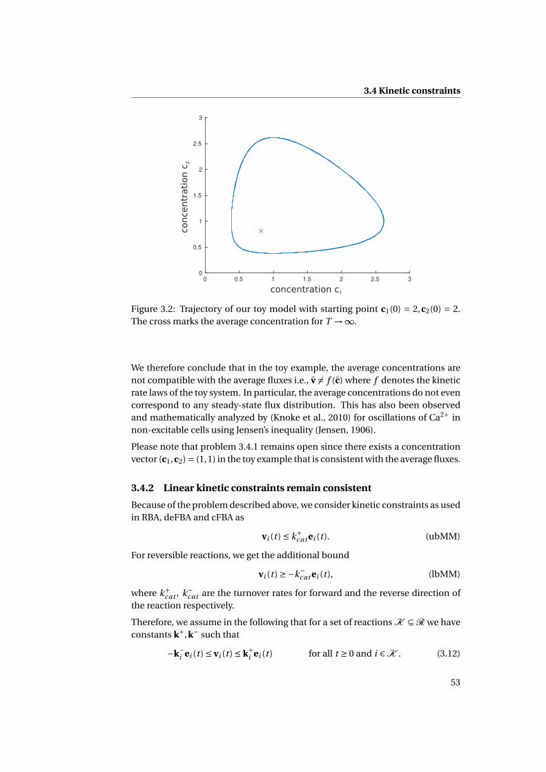
3.4 Kinetic constraints
concentration c1
0 0.5 1 1.5 2 2.5 30
0.5
1
1.5
2
2.5
3
conce
ntr
ati
on c
2
Figure 3.2: Trajectory of our toy model with starting point c1(0) = 2,c2(0) = 2.The cross marks the average concentration for T →∞.
We therefore conclude that in the toy example, the average concentrations arenot compatible with the average fluxes i.e., v 6= f (c) where f denotes the kineticrate laws of the toy system. In particular, the average concentrations do not evencorrespond to any steady-state flux distribution. This has also been observedand mathematically analyzed by (Knoke et al., 2010) for oscillations of Ca2+ innon-excitable cells using Jensen’s inequality (Jensen, 1906).
Please note that problem 3.4.1 remains open since there exists a concentrationvector (c1,c2) = (1,1) in the toy example that is consistent with the average fluxes.
3.4.2 Linear kinetic constraints remain consistent
Because of the problem described above, we consider kinetic constraints as usedin RBA, deFBA and cFBA as
vi (t ) ≤ k+cat ei (t ). (ubMM)
For reversible reactions, we get the additional bound
vi (t ) ≥−k−cat ei (t ), (lbMM)
where k+cat , k−
cat are the turnover rates for forward and the reverse direction ofthe reaction respectively.
Therefore, we assume in the following that for a set of reactions K ⊆R we haveconstants k+,k− such that
−k−i ei (t ) ≤ vi (t ) ≤ k+
i ei (t ) for all t ≥ 0 and i ∈K . (3.12)
53

Chapter 3. Steady states and upper bounds on growth rates from resourceallocation models
This form gives us enough flexibility to also constrain the average fluxes usingthe average enzyme concentrations.
Assuming the average enzyme concentrations e exist, for the linear kinetic con-straints as used in section 3.4.2, we get the following result:
Proposition 3.4.2 Assume v, e exist. Then it holds that
−k−i ei ≤ vi ≤ k+
i ei for all i ∈K . (3.13)
PROOF For the first inequality we have
k+i ei − vi = lim
T→∞k+
i ei (T )− vi (T ) (3.14)
= limT→∞
1
T
∫ T
0k+
i ei (t )−vi (t )d t ≥ 0, (3.15)
because vi (t ) ≤ k+i ei (t ) for all t ≥ 0. Thus, vi ≤ k+
i ei . The same argument alsoapplies to show that −k−
i ei ≤ vi . ■
The case when v, e do not exist is discussed in (Reimers and Reimers, 2016). Thisresult allows us to include enzyme capacity constraints of the type used in RBA,deFBA and cFBA into (FBA1).
3.5 Conclusions
One of the main arguments against using the steady-state assumption in mod-els of biochemical reaction networks is that, if one assumes steady-state, oscil-lations that are biologically important will not be observed in the simulationresults (Goldbeter, 1997; Sowa et al., 2014; Papagiannakis et al., 2017).
3.5.1 Average fluxes satisfy the steady-state assumption
However, in many cases we might not be interested in these oscillations, becausethey increase the complexity of the model, or even make it computationally in-tractable. In these cases, where only average fluxes over long time periods areof interest (e.g. if we are interested in predicting the lethality of gene knockoutexperiments), we have shown that the steady-state assumption can still be ap-plied, i.e., we still get a reasonably good description of the metabolic system bycomputing a steady-state flux. In particular, it is also valid for oscillating systemsthat are not at steady-state at any point in time. The only condition is that thesystem is averaged over a long enough time period.
For example, FBA computes an upper bound on the biomass yield, which ap-plies to all steady-state solutions. Hence it also applies to the average fluxes.Therefore, the system cannot obtain a higher yield using oscillations.
54

3.5 Conclusions
We showed that an average over three hours is sufficient to obtain fluxes thatonly slightly violate the steady-state assumption for E. coli, S. cerevisiae, andHeLa cells. Since the estimate was rather pessimistic, much shorter averagingtimes might be sufficient in practice. Furthermore, the violation we obtainedlies within the error range of current measurement technology for concentra-tions and fluxes.
3.5.2 Pitfalls of averaging
We have seen that, if only average fluxes over long time periods are of interest,the steady-state assumption, is clearly a good model. While this adds anotherargument why methods like FBA can indeed predict the growth rates of someorganisms accurately (Edwards et al., 2001; Harcombe et al., 2013), the integra-tion of nonlinear constraints should be done with care.
For instance, average concentrations might be inconsistent with the averagefluxes. Thus, we cannot exclude that there exists a chemical reaction system(candidates are described in Knoke et al. (2010); Sowa et al. (2014); Gottsteinet al. (2014)) where an oscillation can induce a higher average flux than the fluxthat would be possible by assuming steady-state. We have, however, shown thatlinear constraints, such as those imposed by enzyme availability and enzyme ca-pacity, do not introduce inconsistencies for average concentrations and fluxes.
Since these linear kinetic constraints remain consistent for average concen-trations and fluxes, we could show using averaging why FBA provides upperbounds on biomass yields obtained from resource allocation models. Inaddition, we will see in section 5.3 how, in a similar fashion, RBA provides upperbounds on growth rates from cFBA models. This is a very useful result whendebugging errors in the resource allocation model construction. We now turnour attention in the next chapter to how one constructs such resource allocationmodels.
55


Chapter 4
Building and encoding ametabolic resource allocationmodel
The section on SBML encoding presented in this chapter has been donein collaboration with Henning Lindhorst within the European project RO-BUSTYEAST. The work presented in this chapter has been published inthe journal Metabolites under (Reimers et al., 2017b) and can be found athttp://dx.doi.org/10.3390/metabo7030047. Furthermore, the devel-oped SBML standard has been made available on Fairdomhub as a standardoperating procedure (SOP) at https://www.fairdomhub.org/sops/304.
In this chapter we present a guide for generating a complete (genome-scale)metabolic resource allocation model, as well as a proposal for how to representsuch models in Systems Biology Markup Language (SBML) format. These mod-els lie at the core of resource allocation studies in metabolic networks. To thebest of our knowledge, no guidelines for generating such a model have beenpublished up to now, although the idea of metabolic resource allocation studieshas been present in the field of systems biology for several years.
Therefore, we focus in this chapter on a step-by-step guide towards constructingsuch a model, summarized in figure 4.1, with a focus on the deFBA formalismwhich is described in chapter 2. We detail here all the necessary information aswell as which databases may be used to retrieve it (see table 4.1). To facilitateexchange among researchers, we furthermore propose a standard for specify-ing such models in SBML format using the Flux Balance Constraints extension(Olivier and Bergmann, 2015). Last but not least, we provide some guidelines fordiagnosing possible problems or errors that may arise during the model build-ing process.
57

Chapter 4. Building and encoding a metabolic resource allocation model
4.1 Model prerequisites
(a) annotated genome sequence
amino acids
metabolic network
enzyme
ribosome
ATP, GTP
(c) production of macromolecules by metabolism
RNA
DNA
(d) biomass composition constraints
(b) (genome-scale)metabolic reconstruction
(e) enzyme amount constrains flux (f) match experimental growth rates in constant conditions
20 22 24 26 28-0.5
0
0.5
1
1.5
time t (h)
ln(O
D)
lipids and small molecules
enzymes cell wall
noncatalytic proteins
N C CO
O
H
R
H
H
H
N C CO
O
H
R
H
H
H
N C CO
O
H
R
H
H
H
ncell wall(t) ≥ q · ntotal biomass(t),∀t ≥ 0
v(t) ≤ kcat · nE(t),∀t ≥ 0 data: ln(OD) = µexp · t+ y
model: µmodel =1
tf−t0log
(biomass(tf )biomass(t0)
)
set vmaintenance ≥ 0 s.t. µexp = µmodel
Figure 4.1: Roadmap for generating a deFBA model. From an annotatedgenome sequence (a) of the organism of interest the metabolic network (b)is reconstructed following instructions in (Thiele and Palsson, 2010). Giventhe gene-reaction mapping and the annotated genome sequence, the en-zymes and ribosomes (c), and their synthesis reactions are added to the sto-ichiometric matrix (see Section 4.2). Next, the biomass composition con-straints (d) should be set up using information from the biomass objectivefunction of the metabolic network model (see Section 4.3). Then reactionturnover rates (e) sourced from literature and online databases should be added(see Section 4.4). Lastly but most importantly, the deFBA model should befine tuned to match experimental growth rates (f) obtained in the laboratory(see Section 4.5). Images retrieved from: (a) http://goo.gl/aBNfPz (Skin-ner et al., 2009; Cherry et al., 2012); (b) http://www.genome.jp/kegg-bin/show_pathway?map01100 (Kanehisa and Goto, 2000); (c) http://www.genome.jp/kegg-bin/show_pathway?map01100 (Kanehisa and Goto, 2000), http://pdb101.rcsb.org/motm/10 (Berman et al., 2000), https://swissmodel.expasy.org/repository/uniprot/P04806 (Kiefer et al., 2008).
58

4.1M
od
elprereq
uisites
Table 4.1: Databases where the necessary information needed to build a metabolic resource allocation model can be found.
Resource Link Reference
Annotated genome sequencesGenbank https://www.ncbi.nlm.nih.gov/genbank/ Benson et al. (2013)UniProtKB http://www.uniprot.org/ UniProt Consortium (2014)Metabolic network reconstructionsBiGG http://bigg.ucsd.edu/ King et al. (2016)BioModels https://www.ebi.ac.uk/biomodels-main/ Juty et al. (2015)ModelSEED http://modelseed.org/ Devoid et al. (2013)KEGG http://www.genome.jp/kegg/pathway.html Kanehisa and Goto (2000)Pathway Tools http://bioinformatics.ai.sri.com/ptools/ Karp et al. (2016)Enzyme subunit stoichiometryUniProtKB http://www.uniprot.org/ UniProt Consortium (2014)Ribosome compositionRibosomal Protein Gene Database http://ribosome.med.miyazaki-u.ac.jp/ Nakao et al. (2004)KEGG http://www.genome.jp/kegg/ Kanehisa and Goto (2000)Quantitative proteomics datasetsMaxQuant http://maxqb.biochem.mpg.de/mxdb/ Schaab et al. (2012)Proteomaps https://www.proteomaps.net/index.html Liebermeister et al. (2014)Turnover ratesBRENDA http://www.BRENDA-enzymes.org/ Schomburg et al. (2013)SABIO-RK http://sabio.villa-bosch.de/ Wittig et al. (2012)
59

Chapter 4. Building and encoding a metabolic resource allocation model
The most important prerequisite for building a metabolic resource allocationmodel is a high quality (genome-scale) metabolic reconstruction of the organ-ism of interest. As we will see in the following sections, it is very important thatkey-elements of this reconstruction such as the gene-reaction mapping or thebiomass composition and coefficients are as accurate as possible.
A description of how exactly to come up with such a genome-scale metabolicreconstruction is out of the scope of this chapter. To date, more than 2600 func-tional draft reconstructions have been generated (Büchel et al., 2013) and manyof them can be retrieved from online databases such as BioModels (Le Novèreet al., 2006; Li et al., 2010; Chelliah et al., 2015; Juty et al., 2015). If there existsno genome-scale metabolic reconstruction for the organism of interest, but thefull genome sequence of the organism is available, the protocol of (Thiele andPalsson, 2010) can be followed in order to generate the metabolic network re-construction.
Note that, depending on the organism, it may not be possible to simulate acomplete genome-scale deFBA model due to the size of the resulting linearprogram. While RBA allows simulation of steady-state resource allocation ingenome-scale networks (Goelzer and Fromion, 2017), the dynamic approacheslike deFBA are constrained to smaller sizes. Networks with up to 500 metabolicreactions can be successfully simulated with deFBA as demonstrated in(Reimers et al., 2017a). If the starting metabolic network is too large, tools suchas the minimal network finder in (Röhl and Bockmayr, 2017) or the proceduresin (Erdrich et al., 2015; Ataman et al., 2017) can be used to reduce the size of thenetwork while at the same time keeping desired functionalities.
Another key prerequisite of a deFBA model are the annotated amino acid se-quences of all the genes present in the model, as we will explain next.
4.2 Building the protein production reactionsAny good quality genome-scale metabolic reconstruction comes with a gene-reaction mapping. Such a mapping describes exactly what genes are involvedin the catalysis of each reaction. In addition, it also offers information aboutisoenzymes, i.e., enzymes that differ in amino acid sequence but catalyze thesame reaction. In the following subsections we will explain how to make use ofthe gene-reaction mapping in order to construct the protein production reac-tions for a deFBA model.
4.2.1 The case of enzymes encoded by one gene only
To build any protein production reaction using the gene-reaction mapping thekey ingredient is a database of all genes and their corresponding amino acidsequences. This can be obtained as a FASTA file from online databases suchas Genbank (Benson et al., 2013) or UniProt (UniProt Consortium, 2017). A
60

4.2 Building the protein production reactions
FASTA file is a file formatted such that it represents either nucleotide or pep-tide sequences using single-letter codes. The advantage of using UniProt is that,through the Java API (http://www.ebi.ac.uk/uniprot/japi/usage.html),one can automatically access the sequences, as well as information about theEnzyme Commission number (EC number) or subunit stoichiometry for en-zymes. There also exist organism-specific databases where this information canbe retrieved. To give some examples, in the case of Saccharomyces cerevisiae onecould obtain such a FASTA file also from the Saccharomyces Genome Database(Cherry et al., 2012), while for cyanobacteria one could use Cyanobase (Nakaoet al., 2010).
To then build the enzyme production reaction for an enzyme encoded by onegene only, we look up the corresponding gene in the FASTA file, compute itsamino acid count, and set the amino acids with their respective counts as re-actants for the production reaction. Additional reactants are then the energycofactors needed to grow the peptide chain: per amino acid added, one ATPis hydrolyzed into AMP and PPi, and two GTP molecules are hydrolyzed intoGDP and Pi. Last but not least, for the translation initiation a molecule of 10-formyltetrahydrofolate (fTHF) is converted into a molecule of tetrahydrofolate(THF) (Nelson et al., 2008).
Another important factor that comes into play is then also whether the enzymeis a monomer, i.e., if only one copy of the corresponding gene product is neededto build the enzyme. If this is not the case, then the amount of copies of thegene product required to produce the enzyme has to be accounted for in theproduction reaction. This information can be often retrieved from the UniProtdatabase. As an example, if the enzyme is a homotrimer, i.e., three copies of thegene product are needed to build it, then the stoichiometries of the amino acidsand the energy cofactors in the production reaction have to be multiplied bythree. The importance of taking into account such information can be seen inthe cost of producing such an enzyme. Not taking into account such extra costscan result in wrong predictions in the use of alternative pathways.
4.2.2 The case of isoenzymes
Isoenzymes usually arise as a result of partial genome duplication and subse-quent point mutations or insertion/deletion events in the course of evolution.They usually have different kinetic properties and are subject to different regu-latory influences. Isoenzymes are important features of metabolism that allowfine-tuning of reactions rates in a way that satisfies the exact needs of the organ-ism at different stages of development or of the cell cycle. An example of suchpairs of enzymes are glucokinase and hexokinase, which both catalyze the con-version of a hexose into a hexose 6-phosphate. While hexokinase is inhibitedby glucose 6-phosphate, glucokinase is not. This different regulatory feature,together with its lower affinity for glucose, allows glucokinase to play different
61
Chapter 4. Building and encoding a metabolic resource allocation model
roles in cells of specific organs.
Isoenzymes also play a special role in a deFBA model. To see this, let us as-sume we have two enzymes e1 and e2 that catalyze the same reaction r . In thedeFBA model we would then build two enzyme production reactions with dif-ferent amino acid requirements for the two enzymes and then the sum of theamounts of these enzymes will bound the flux through reaction r together withthe corresponding turnover rates.
Having mentioned turnover rates, it is important to keep in mind that usuallyisoenzymes are assigned the same EC number. This means that, when search-ing turnover rates for isoenzymes we are usually bound to find the same val-ues in databases such as BRENDA (Schomburg et al., 2013), although in realitythe turnover rates may be different. This is partially due to the EC number be-ing a bad standard, but also partly due to lack of biochemical data on differentenzyme isoforms. This fact results in isoenzymes most often having the samecatalytic efficiency in a deFBA model.
Therefore, the only distinguishing feature of isoenzymes from the perspective ofresource allocation, is their amino acid cost. The amino acid cost is not a de-fined concept. It can be understood in several ways: the length of the enzymesequence in amino acids or the amount of energy in the form of ATP needed tobuild all the amino acids in the enzyme or the number of carbon molecules in-vested in building all the amino acids for an enzyme. If we think of the aminoacid cost of an enzyme in terms of the length of the sequence, then if the twoisoenzymes have the same length, which of them will be in the end be producedin the deFBA model strongly depends on the requirements of the rest of the sys-tem in terms of amino acids at that particular time point. On the other hand,if the lengths of the two isoenzymes are different, very often the deFBA modelwill predict that only the enzyme with the shorter sequence will be producedand used. This points out two aspects: (i) the system can be simplified by sim-ply not considering at all the more expensive enzyme and this way sparing inthe number of variables and the solving time, and (ii) it may be that the regula-tory structure of the cell actually has a strong impact on whether these enzymesare produced in reality, but since deFBA ignores this regulatory structure it maymispredict the usage of these enzymes.
Last but not least, which isoenzyme is used may also be dependent on the ex-tracellular conditions in which the cell lives. In this case, even if usually shorter(and hence very likely cheaper) enzymes are preferred, it can still be that theenvironment turns this decision around and gives rise to a different resource al-location scheme. Therefore, if they do not make a significant difference in thecomplexity of the resulting linear program, it is recommended that all isoen-zymes are represented in the resource allocation model.
The way the isoenzyme production reactions are built depends on their subunitstructure. If each of them is only encoded by one gene, then we proceed as in
62

4.2 Building the protein production reactions
subsection 4.2.1 above. If several genes are needed to encode one of the isoen-zymes, then the respective isoenzyme production reaction will have all aminoacids of all involved gene products as substrate requirements, as described insubsection 4.2.3 below.
4.2.3 The case of enzyme complexes encoded by several genes
Suppose we want to build the production reaction for an enzyme encoded by thecombination of three gene products, g1, g2, and g3. The metabolic model en-codes this as the gene rule for the respective reaction being “g1 AND g2 AND g3”.In this case, we compute the amino acid counts for all three genes, add them upand use them as reactants as described in subsection 4.2.1, while making surewe also adapt the ATP and GTP requirements.
This strategy is however only correct in the case in which the peptides encodedby each gene participate in the enzyme as monomers. This is not always thecase, and often peptides encoded by one gene participate in enzymes as dimersor trimers, as is the case for example in ATPase, where subunit alpha participatesas trimer. Therefore, it is often the case that, before we add up the amino acidcounts for all genes, we have to multiply some of the counts with the factor withwhich they participate in the enzyme.
Information about the stoichiometry of individual peptides within enzymes isunfortunately not readily incorporated in genome-scale metabolic reconstruc-tions and can often only be found through extensive literature research or byquerying the UniProt database. Failing to incorporate such stoichiometric in-formation is very likely to give rise to false computational predictions due to thedifferent tradeoffs arising from incorrect enzyme energetic cost.
4.2.4 The ribosome
In deFBA models, the ribosome is assumed to simply have catalytic functionjust as any other enzyme. The amount of ribosome bounds the combined fluxesthrough the protein production reactions via different turnover rates.
Ribosome production
Considering the ribosome to be an “enzyme” encoded by several genes, its pro-duction reaction can be modeled as described in subsection 4.2.3 above. As op-posed to usual enzymes for which it may be difficult to find the stoichiometryof individual peptides, the ribosomes are rather well studied and informationabout their composition can be found for many organisms in the Kyoto Ency-clopedia of Genes and Genomes (KEGG) (Kanehisa and Goto, 2000) or in theRibosomal Protein Gene Database (Nakao et al., 2004). In addition to the ribo-somal proteins, also the ribosomal RNA needs to be taken into account for the
63

Chapter 4. Building and encoding a metabolic resource allocation model
production reaction. Information about this can also be found in the KEGG re-source.
Ribosome translation rate
The ribosome translation rate is a key parameter in a deFBA model and it hasvery high impact on the tradeoffs that govern the choice of one model behav-ior over another. This parameter directly affects the enzymatic cost of differentpathways.
Ribosome translation rates vary between prokaryotes and eukaryotes and theyeven vary with growth rate within the same organism (Bremer and Dennis,2008). They are usually measured in attached amino acids per second, andhence the efficiency of the ribosome for building different enzymes is de-pendent on this parameter, but also on the respective enzymes’ lengths. Forinstance, if we consider the translation of one enzyme of 100 amino acids by abacterial ribosome with a rate of 15 amino acids per second then, assuming theenzyme does not compete with other proteins for the ribosome, the enzymewill be translated at a maximal rate of 3600 ·15/100 = 540 enzymes per hour. Ingeneral the formula for computing the kcat of the ribosome for the productionof a protein is thus given by
kcat = 3600r
l,
where r is the ribosome rate in amino acids per second, and l is the length ofthe protein in amino acids. In this way we can assign all protein productionturnover rates, including those of the protein quota, by using the protein aminoacid length, which is the sum of the stoichiometries of the amino acids in theprotein production reaction.
4.2.5 Compartmentalization
Eukaryotic cells, as opposed to prokaryotic ones, are usually compartmental-ized, with compartments such as cytosol, mitochondrion etc. This compart-mentalization plays a role in the way enzymes are built, in the sense that theremay be identical enzymes that are active in the cytosol as well as in the mito-chondrion for example. In this case, two production reactions should be used,one for each compartment, since an enzyme that is in the cytosol cannot cat-alyze a reaction in the mitochondrion.
4.3 Setting up quota compounds and storageAlthough the catalytic biomass is the main part of the model that is responsiblefor the autocatalytic cycle, there are several noncatalytic macromolecules thatare also needed in a full cell model. Examples are DNA, RNA, cell wall or mem-brane. Without accounting for the growth and duplication of these components,
64
4.3 Setting up quota compounds and storage
we would not be modeling a whole copy of a cell and we would be neglectinga significant biosynthetic energy requirement. We recall that we have namedthese macromolecules quota metabolites, to reflect the fact that a certain quotaof the total biomass needs to be dedicated to them.
In the case of a periodic environment as is the case for cyanobacteria, algae orplants for example, the production of quota compounds can be enforced by im-posing initial quota amounts and requiring that these amounts grow at the samerate as the catalytic biomass, as done in the cFBA model in chapter 6.
In case the environment is not periodic, the simulation can be started by im-posing these quota components to make up a certain percentage of total initialbiomass, and that these percentages are then kept throughout all the time pointsof the solution. The question then arises: what are appropriate initial amountsfor these quota components?
4.3.1 Initial quota compound amounts
A good place to look for initial quota amounts is the biomass reaction of themetabolic network reconstruction. The stoichiometric coefficients for the reac-tants of this artificial reaction describe the average composition of the modeledcell. To better understand this, let us take a look at the biomass reaction of theYeast 6.06 model which we have reproduced in table 4.2.
We observe here the main biomass components: proteins (in the form ofcharged transfer RNAs), storage (glycogen and trehalose), DNA (in the form ofdAMP, dCMP, dGMP, dTMP), RNA (AMP, CMP, GMP, UMP), cell wall (mannanand β-D-glucan), membrane (lumped lipid), other small molecules, and theATP energy needed for polymerization. For ease of understanding later on,we denote the biomass reaction by b, the indices of biomass components(reactants of biomass reaction) as Ibio, and the indices of biomass byproducts(products of biomass reaction) as Ibp. Then the biomass reaction has the form∑
i∈Ibio
Si bMi → 1 biomass+ ∑i∈Ibp
Si bMi .
In general, the reactant stoichiometries for the biomass reaction are chosensuch that, when weighted by the corresponding molecular weights (MW), theyadd up to 1, i.e., ∑
i∈Ibio
Si bMWi −∑
i∈Ibp
Si bMWi = 1.
In other words, we can look at the reactant stoichiometries, multiplied by themolecular weights, as the fractions qi := Si bMWi of the respective metaboliteswithin one cell, or equivalently one gram dry weight of cells. Hence, these canalso be used as initial quota amounts.
65

Chapter 4. Building and encoding a metabolic resource allocation model
Table 4.2: Biomass reaction of the Yeast 6.06 model.
Reactants Stoichiometry Products Stoichiometry
Ala-tRNA(Ala) 0.4588 tRNA(Ala) 0.4588Arg-tRNA(Arg) 0.1607 tRNA(Arg) 0.1607Asn-tRNA(Asn) 0.1017 tRNA(Asn) 0.1017Asp-tRNA(Asp) 0.2975 tRNA(Asp) 0.2975Cys-tRNA(Cys) 0.0066 tRNA(Cys) 0.0066Gln-tRNA(Gln) 0.1054 tRNA(Gln) 0.1054Glu-tRNA(Glu) 0.3018 tRNA(Glu) 0.3018Gly-tRNA(Gly) 0.2904 tRNA(Gly) 0.2904His-tRNA(His) 0.0663 tRNA(His) 0.0663Ile-tRNA(Ile) 0.1927 tRNA(Ile) 0.1927Leu-tRNA(Leu) 0.2964 tRNA(Leu) 0.2964Lys-tRNA(Lys) 0.2862 tRNA(Lys) 0.2862Met-tRNA(Met) 0.0507 tRNA(Met) 0.0507Phe-tRNA(Phe) 0.1339 tRNA(Phe) 0.1339Pro-tRNA(Pro) 0.1647 tRNA(Pro) 0.1647Ser-tRNA(Ser) 0.1854 tRNA(Ser) 0.1854Thr-tRNA(Thr) 0.1914 tRNA(Thr) 0.1914Trp-tRNA(Trp) 0.0284 tRNA(Trp) 0.0284Tyr-tRNA(Tyr) 0.1020 tRNA(Tyr) 0.1020Val-tRNA(Val) 0.2646 tRNA(Val) 0.2646ATP 59.2760 ADP 59.2760H2O 59.2760 phosphate 58.70001(1→3)-β-D-glucan 1.1348 H+ 59.3050(1→6)-β-D-glucan 1.1348 biomass 1glycogen 0.5185trehalose 0.0234mannan 0.8079riboflavin 0.00099lipid 1sulphate 0.0200dAMP 0.0036dCMP 0.0024dGMP 0.0024dTMP 0.0036AMP 0.0460CMP 0.0447GMP 0.0460UMP 0.0599
66

4.3 Setting up quota compounds and storage
To help reduce the number of quota compounds we model and also the sizeof the resulting resource allocation problems, we can build helper spontaneousreactions that consume the metabolites above and produce the needed quotacompounds. As an example, all charged transfer RNAs (whose indices we denoteby Iaa−tRNA ⊂ Ibio) would be consumed to produce one merged protein quotacompound, and release all the uncharged tRNAs (indices denoted by ItRNA ⊂Ibp). In setting up this reaction, we should make sure that we adjust the sto-ichiometric coefficients in such a way that, multiplied with the correspondingamino acids’ molecular weights, they add up to one, i.e., we need to divide themby
qprotein = ∑i∈Iaa−tRNA
Si bMWi .
Thus, the protein quota building reaction will read
∑i∈Iaa−tRNA
Si b
qproteinMi + SATP b
qproteinATP+ SH2O b
qproteinH2O
→ 1 protein+ ∑i∈ItRNA
Si b
qproteinMi + SADP b
qproteinADP+ Sphosphate b
qproteinphosphate+ SH+ b
qproteinH+.
For the protein quota in Yeast 6.06, we can compute from table 4.2 qprotein =0.466298. Therefore, the corresponding quota production reaction would thenlook as shown in table 4.3. The necessary ATP needed for polymerization, whichis the fraction qprotein of the total ATP consumed in the original biomass reaction,is also part of this reaction.
After setting up this reaction, the required initial amount of protein quota isqprotein. However, of these proteins, some are modeled explicitly as enzymes,and in the next section we will see how to adjust the qprotein to only require theproteins that are not modeled as enzymes or ribosome. For the rest of the quotacompounds (DNA, RNA, cell wall, membrane, other small molecules) we wouldproceed in a similar fashion as for the proteins, with the sole difference that theirq would not need to be adjusted once computed.
4.3.2 The case of noncatalytic proteins
The noncatalytic proteins quota is a special case because, in typical biomassreactions, we only have one protein component which encompasses all proteincontent present in one gram dry weight of cells. However, we need to distinguishin a deFBA model between proteins with catalytic role, and those without, andthus to find a way of splitting this percentage, since obviously the cell containsother proteins besides those we model individually as enzymes.
One way to do this is find a (genome-scale) quantitative proteomics dataset. Ifnot already scaled, we normalize the protein amounts in the dataset to add up to
67

Chapter 4. Building and encoding a metabolic resource allocation model
Table 4.3: Helper reaction for producing the protein quota in the Yeast 6.06model.
Reactants Stoichiometry Products Stoichiometry
Ala-tRNA(Ala) 0.9839201541 tRNA(Ala) 0.9839201541Arg-tRNA(Arg) 0.3446294001 tRNA(Arg) 0.3446294001Asn-tRNA(Asn) 0.2181008711 tRNA(Asn) 0.2181008711Asp-tRNA(Asp) 0.6380040232 tRNA(Asp) 0.6380040232Cys-tRNA(Cys) 0.0141540388 tRNA(Cys) 0.0141540388Gln-tRNA(Gln) 0.2260357111 tRNA(Gln) 0.2260357111Glu-tRNA(Glu) 0.6472255939 tRNA(Glu) 0.6472255939Gly-tRNA(Gly) 0.6227777087 tRNA(Gly) 0.6227777087His-tRNA(His) 0.1421837537 tRNA(His) 0.1421837537Ile-tRNA(Ile) 0.4132550429 tRNA(Ile) 0.4132550429Leu-tRNA(Leu) 0.6356450167 tRNA(Leu) 0.6356450167Lys-tRNA(Lys) 0.6137705931 tRNA(Lys) 0.6137705931Met-tRNA(Met) 0.1087287529 tRNA(Met) 0.1087287529Phe-tRNA(Phe) 0.2871554242 tRNA(Phe) 0.2871554242Pro-tRNA(Pro) 0.3532076054 tRNA(Pro) 0.3532076054Ser-tRNA(Ser) 0.3975998181 tRNA(Ser) 0.3975998181Thr-tRNA(Thr) 0.4104671262 tRNA(Thr) 0.4104671262Trp-tRNA(Trp) 0.060905258 tRNA(Trp) 0.060905258Tyr-tRNA(Tyr) 0.2187442365 tRNA(Tyr) 0.2187442365Val-tRNA(Val) 0.5674482841 tRNA(Val) 0.5674482841ATP 36.3823134562 ADP 36.3823134562H2O 36.3823134562 phosphate 36.3823134562
H+ 36.3823134562protein 1
one. We observe that in this dataset we find two types of proteins correspondingto our model: those modeled explicitly as enzymes, which sum up to a fractionfe , and those not present explicitly in our model, that we call quota proteins,and which sum up to 1− fe after the normalization of the dataset.
Since we want to adapt the protein quota to only account for the noncatalyticproteins, we adjust qprotein by multiplying it with the fraction 1− fe of noncat-alytic proteins in the dataset.
An important point here is the growth rate at which the cells used for the quanti-tative proteomics measurement were growing. It has been shown already in sev-eral studies that, for instance, the total amount of ribosomes grows linearly withthe growth rate and that partitioning of proteome strongly varies with growthrate and growth conditions (Klumpp et al., 2009; Scott et al., 2010, 2014). SincedeFBA models an autocatalytic system that grows exponentially, quantitative
68

4.4 Assigning reaction turnover rates
proteomics datasets from exponentially growing cultures should be used if avail-able.
4.3.3 Storage
Besides the catalytic and quota macromolecules, most organisms also have stor-age macromolecules. For some of them, like cyanobacteria, the storage is essen-tial to survive over the night period, when no energy from the sun is present. Forothers, like yeast, the storage is useful to survive through periods of starvation,as well as sudden changes in the nutrient landscape, when new enzymes andtransporters have to be synthesized in order to survive. Therefore, it is impor-tant that a resource allocation model takes such storage macromolecules intoaccount.
Taking a second look at the biomass reaction of Yeast 6.06 in table 4.2, weobserve that glycogen and trehalose are also consumed. We have howevernot added them as quota compounds, because these are the storage macro-molecules of yeast. Therefore, we allow these macromolecules to accumulate ina deFBA model, the same way as proteins. Moreover, they are part of the totalbiomass used as objective and to constrain the quota amounts. However, thereis no reason why we should impose an initial amount for the storage. We stillallow that initial storage amount is present by constraining the total biomass atthe beginning of the simulation to be equal to 1 gram. In this way, storage maybe present at the beginning, but at the expense of having less catalytic biomass.
4.4 Assigning reaction turnover ratesTurnover rates are necessary parameters in a resource allocation model. Theyare involved in the capacity constraints that bound reaction fluxes using theamount of their catalyzing enzymes. A recent study has shown that turnovernumbers reported in online databases are a good enough approximation of invivo turnover numbers (Davidi et al., 2016).
The two main databases for retrieving turnover numbers are BRENDA (Schom-burg et al., 2013) and SABIO-RK (Wittig et al., 2012). While BRENDA offers bothmanually curated as well as text mining data, SABIO-RK only offers data thatwas either manually extracted from the literature or directly submitted by ex-perimenters. As a result, BRENDA offers a larger amount of turnover rates thanSABIO-RK. Both databases offer automated retrieval options. Some simple rulesof thumb for retrieving turnover rates from these databases are that one shouldfilter for wild type, non-recombinant values, and, if possible, should make surethat the measurements were done at (nearly) physiological pH and temperaturevalues.
Although large amounts of biochemical data are now available, not all turnoverrates for the organism of interest can be found. We recommend in this case, if
69

Chapter 4. Building and encoding a metabolic resource allocation model
turnover rates for a given enzyme from other organisms are found, that theseshould be used. The question then arises: which of the available turnover ratesshould be used? Should it be a mean or a median of all found turnover rates, orthe turnover rate from the organism that has the most sequence similarity withthe target organism within that protein?
To answer this question, we have automatically retrieved wild type turnoverrates from the BRENDA database for all enzymes from three organisms: Sac-charomyces cerevisiae, Escherichia coli, and Bacillus subtilis. In a second iter-ation, we retrieved turnover rates of all enzymes from all other organisms, ex-cluding the organism of interest, and computed the mean, median, and bestsequence match with the organism of interest kcat . The best sequence matchwas obtained by computing the alignment score using the Needleman-Wunschalgorithm (Needleman and Wunsch, 1970) with the BLOSUM62 scoring matrix(Henikoff and Henikoff, 1992). Since we mostly want that the order of magni-tude of the turnover rates is correct, we computed the Pearson correlation coef-ficients between the logarithms of kcat values from the organism of interest andthe logarithms of the mean, median and best sequence match kcat values ob-tained from other organisms. Only values corresponding to the same enzymeswere compared. The resulting correlation coefficients are displayed in table 4.4.
Table 4.4: Pearson correlation coefficients between the logarithms of kcat valuesfrom the organism of interest and the logarithms of the mean, median and bestsequence match kcat values obtained from other organisms.
Organism median mean best sequence match
Saccharomyces cerevisiae 0.701 0.650 0.526Escherichia coli 0.808 0.756 0.606Bacillus subtilis 0.762 0.708 0.679
We observe that, in the cases we have analyzed, the medians of all turnover ratesenzyme-wise is the best approximation for the actual turnover numbers in theorganism of interest. Moreover, the order of magnitude correlation coefficientsare very high and the P-values we get are all in the order of 10−14 or lower, indi-cating that indeed these median turnover rates from other organisms are goodenough approximations of the real kcat values if no specific data is available forthe organism of interest.
To give an idea of the spread of the turnover rate data, we show in figure 4.2 a plotof the kcat values in yeast versus the median kcat values from other organisms.
4.5 Validating the model using experimental dataOnce the model has been constructed, a first step before further investigations isits validation using experimental data. This can stretch from fairly basic match-
70

4.5 Validating the model using experimental data
10-6 10-4 10-2 100 102 104 106
median kcat
of enzyme from other organisms
10-6
10-4
10-2
100
102
104
106
kca
t of
enzy
me in
S. ce
revis
iae
Figure 4.2: Turnover rates in yeast versus the median kcat values from other or-ganisms.
ing of growth rates obtained from batch experiments to matching of reactionfluxes if data is available.
In general, the growth rate obtained in the model under constant conditionsshould provide an upper bound on the growth rate measured in the lab, sincethe model gives the optimal behavior of the metabolism, which may not alwaysbe observed in the lab. To check that this is the case, we need data from an expo-nentially growing batch culture of the organism of interest at saturating nutrientconcentrations. In this case, it is sufficient to compute the growth rate of theculture µexp as the slope of the logarithm of the optical density (OD) measure-ments versus time, as in figure 4.1. In addition, we also need to compute theinstantaneous growth rate of the model (under the same conditions as in theexperiments), which we define as
µmodel(t ) := 1
ti+1 − tiln
(biomass(ti+1)
biomass(ti )
), ∀t ∈ (ti , ti+1). (4.1)
We observe that, if nutrients are saturating, µmodel(t ) is constant, and hence wewill refer to it in this case as simply µmodel.
We note that this definition is nearly identical to the growth rate definition inequation (2.2). It is however based on mass and not on volume, and thus as-sumes that the mass grows exponentially. Therefore, with a slight abuse of no-tation and by assuming the density of the cell remains constant, we will use thesame letter µ to denote the mass-based growth rate.
If µmodel is smaller than µexp, the problem lies very likely in the kcat values andthese should then be checked manually. If this is not the case, µmodel can be
71

Chapter 4. Building and encoding a metabolic resource allocation model
tuned to µexp by forcing flux through the ATP maintenance reaction1, which hy-drolyzes ATP into ADP and phosphate. This makes sense also from a biologicalperspective, since we cannot claim that our resource allocation model covers allenergy expending processes in an actual cell, so the ATP maintenance reactionserves the purpose of modeling this remaining energy expenditure.
4.6 Units
One very important aspect in the model building process are the units, as mis-matches between them nearly always give rise to either infeasible or incorrectcomputational results. Therefore, in this section we will elaborate on the unitsof the quantities in a deFBA model.
4.6.1 Metabolic reactions
Metabolic reactions r , including the exchange reactions, are in general of theform
r :∑
iSi r Xi →
∑j
S j r X j ,
where Xi , X j are metabolic reactants resp. products and Si r ,S j r are their stoi-chiometric coefficients in reaction r .
As it is usually the case in metabolic network reconstructions, the unit of the fluxthrough this reaction is mmol
gDW ·h . This information can be found in the SBML fileof the metabolic network reconstruction. However, methods such as deFBA usemolar amounts, and thus the gDW part is not present, so the fluxes there are inmmol
h .
Since the derivative of the molar amount of a metabolite participating in thisreaction has to have the same unit as the flux, it follows that the internal andexternal metabolite amounts are measured in mmol.
The unit of the turnover rates of these reactions is h−1.
4.6.2 Reactions producing quota compounds
In some metabolic network reconstructions artificial reactions are addedto form each biomass component. These biomass components are then inturn consumed by the biomass reaction. This is for instance the case for theSynechococcus elongatus model in chapter 6. These reactions have the general
1Note that the flux we need to force through maintenance strongly depends on how detailedthe model is and how much lumping of reactions has been done. We therefore cannot provide anorder of magnitude approximation for how much flux should be forced. Modelers should howeverbe aware that the need for a large ATP maintenance forced flux to match experimental growthrates is an indication of model errors or poor model quality.
72

4.6 Units
formr :
∑i
Si r Xi → 1g B j ,
where Xi are internal metabolites, B j is an artificial metabolite that representsa quota macromolecule (e.g. membrane), and Si r are corresponding stoichio-metric coefficients, as explained in section 4.2. The coefficients Si r are chosensuch that, when multiplied with the molecular weights of the metabolites Xi ,their sum amounts to 1 gram.
The unit of the flux through such a reaction is then h−1. The amounts of themetabolites Xi are measured in mmol, and the amount of B j is measured in g .The reactions producing quota compounds are artificial reactions, and hence inthe deFBA model they are marked as spontaneous, i.e., no enzyme is needed fortheir catalysis.
The biomass reaction of the metabolic reconstruction then has the form
r :∑
iSi r Bi → Bio,
where Bi are the artificial metabolites that represent quota macromolecules andBio is then the biomass itself, measured in grams. The coefficients Si r are thenchosen such that they represent the fractions of the respective macromoleculesin one gram dry weight of cells. The flux through this reaction is measured inh−1.
While this biomass reaction is not of direct interest in the case of deFBA mod-els, its coefficients Si r are used as initial quota compound amounts and thewhole simulation is set such that at the beginning we are looking at one gramdry weight of cells.
A special case arises here: the quota reaction producing nonmetabolic proteins.This reaction is not spontaneous, but it is catalyzed by the ribosome and com-petes this way for the ribosome with the enzyme production reactions. Thus, wehave to compute a turnover rate for it as described in section 4.3 above. The unitof this turnover rate however is not h−1, but 1
mmol·h .
4.6.3 Reactions producing enzymes
Enzyme production reactions have the form
r :20∑
i=1Si ,r Ai +d1ATP+d2GTP+fTHF → E +d1AMP+d1PPi+d2GDP+d2Pi+THF,
where A1, . . . , A20 are the 20 proteinogenic amino acids, E is the produced en-zyme, and Si ,r , d1 := ∑20
i=1 Si ,r , d2 := 2 ·d1 are the stoichiometric coefficients ofthe amino acids and energy requirements, set up as described in section 4.2.
The flux, molar amounts, and turnover rate units for such reactions are the sameas the ones for metabolic reactions.
73

Chapter 4. Building and encoding a metabolic resource allocation model
4.7 Debugging the model
Even if one follows very carefully the steps we have described above, it is rarelythe case that the model building process ends here. Typically, one needs addi-tional efforts for “debugging” errors.
One example of such an error is that, when simulating growth in a simple en-vironment without any limiting nutrients using cFBA, the resulting LP problemis infeasible. If this happens, one should try to analyze the simplest possiblecase: constant environment, one discretization time step. As we will see in chap-ter 5, this is equivalent to solving an RBA model. This results in the smallestproblem size, since the problem size typically grows linearly with the number ofdiscretization points. In this simplest setting, one can then use the tools of LPsolvers to compute an irreducible inconsistent subsystem (IIS) and get an ideaabout which constraints are involved in the infeasibility. An IIS is a subset ofthe constraints and variable bounds of the LP. Removing any constraint of theIIS from the LP produces a feasible result. Standard commercial LP solvers likeCPLEX or Gurobi offer tools for computing IIS. The type of constraints involvedin the IIS could then help diagnose the infeasibility.
A similar problem can be found in a deFBA model simulated in a simple envi-ronment without nutrient limitations, with the difference that the resulting LPis not infeasible, but instead no biomass growth is obtained. One can approachthis problem in a similar way as above, by forcing a small flux through the ri-bosome production reaction using a positive lower bound for instance. This willthen very likely result in an infeasible LP that can be approached, as above, usingthe IIS.
However, not too much time should be spent on exploring the IIS because it mayhappen that there is actually nothing wrong with the model. In other words, thenumerical instabilities may be the reason for an infeasibility. It is therefore worthtrying to solve the LP also with a more accurate LP solver that can perform itera-tive refinement, such as SoPlex (Wunderling, 1996; Gleixner et al., 2012, 2016). Ifa feasible solution is obtained this way, then numerical problems are the causeof the infeasibility.
Last but not least, it is also worth checking that all quota compounds can beproduced. If this is not the case, this may be a reason for the infeasibility. Tocheck that each quota compound can be produced, simply require them one byone and solve the resulting LPs.
It can sometimes also happen that the LP problem is feasible, but the resultingtime courses reveal problems of the solution. We mention here two typesof problems: (i) non-smoothness/instabilities of the time courses of stor-age/biomass components, and (ii) significantly high amounts of a few of theenzymes. In the former case, the discretization of the dynamic variables maybe faulty, as we will see in the next chapter. In the latter case, it may be that
74

4.8 The SBML representation of a metabolic resource allocation model
the turnover numbers of those enzymes are not correct. Typically few enoughenzymes show this problem, so one can simply check those turnover ratesmanually and look up alternatives in the databases.
4.8 The SBML representation of a metabolic resource al-location model
For metabolic network models used together with constraint-based modeling, itis standard to define them in the systems biology markup language (SBML), anXML-based way of representing models (http://sbml.org/Main_Page). How-ever, there is so far no specific way of representing resource allocation models,which come with several extra ingredients in addition to the metabolic networkpart. Therefore, in this section we propose a way of making use of the existingSBML capabilities for representing resource allocation models. We illustrate thisproposal using a toy resource allocation model listed in table 4.5 for which weattach the SBML representation in Appendix B.
4.8.1 Compartments
We keep any compartments present from the original reconstruction of themetabolic network. If possible, we place the gene products in the compart-ments in which they are acting. This means for instance that enzymes arelocated where the reactions they are catalyzing are happening. Species withoutany real physical location in the model, e.g. quota compounds, can be placedarbitrarily in any compartment.
4.8.2 Species
Each species (metabolite or macromolecule) must contain the fields:
• id• compartment• constant (true or false)• boundaryCondition (true or false)• initialAmount
Depending on the function of the species in the model, it also contains aram:species annotation.
We distinguish between limiting extracellular metabolites (N1 and N2), nonlim-iting extracellular metabolites (O2), intracellular metabolites (N, AA, ATP), stor-age (Stor), and biomass components (ETrans1, ETrans2, Complex_1, EMetab1,EMetab2, EStor, S, R).
The parameters constant and boundaryCondition are used to expresswhether a species is intracellular (constant = “false” boundaryCondition =
75

Chapter 4. Building and encoding a metabolic resource allocation model
Table 4.5: List of species, reactions, and catalysis relationships for the toy modelwhose SBML representation can be found in Appendix B. The reaction that con-sumes AA and ATP but produces nothing is the maintenance reaction and isconsidered spontaneous. The reaction that produces the storage compoundStor has different turnover numbers for the forward (f) and reverse (r) directions.Complex_1 is a transporter complex composed of ETrans1 and ETrans2. S is astructural quota component and R is the ribosome.
External metabolites: N1, N2, O2
Internal metabolites: N, AA, ATPMacromolecules: Stor, ETrans1, ETrans2, Complex_1,
EMetab1, EMetab2, EStor, S, R
Reactions Catalysed by Turnover rateN1 + O2 ↔ N ETrans1 1800N2 ↔ N Complex_1 2400N → AA + ATP EMetab1 2000N → AA + ATP EMetab2 2500N → AA + 2 ATP EMetab2 200050 AA + 60 ATP →∅200 AA + 300 ATP ↔ Stor EStor f: 25, r: 30100 AA + 450 ATP → ETrans1 R 1060 AA + 270 ATP → ETrans2 R 16.67160 AA + 720 ATP → Complex_1 R 6.25200 AA + 900 ATP → EMetab1 R 5160 AA + 720 ATP → EMetab2 R 6.25150 AA + 500 ATP → EStor R 51500 AA + 200 ATP → S R 101000 AA + 4500 ATP → R R 1
“false”), whether it is part of the environment and assumed to be present inabundance (constant = “true” boundaryCondition = “true”), or whetherthe species is a limiting nutrient (constant = “false” boundaryCondition =“true”). We show in Table 4.6 examples on how to set the mandatory speciesfields for each of these metabolite types.
Table 4.6: Examples for setting species fields for each species type.
id compartment constant boundaryCondition initialAmount
N1 N1 external false false 10O2 O2 external true true 10N N metabolites false false 0Stor Stor storage false false 0R R bio false false 0.03364
76
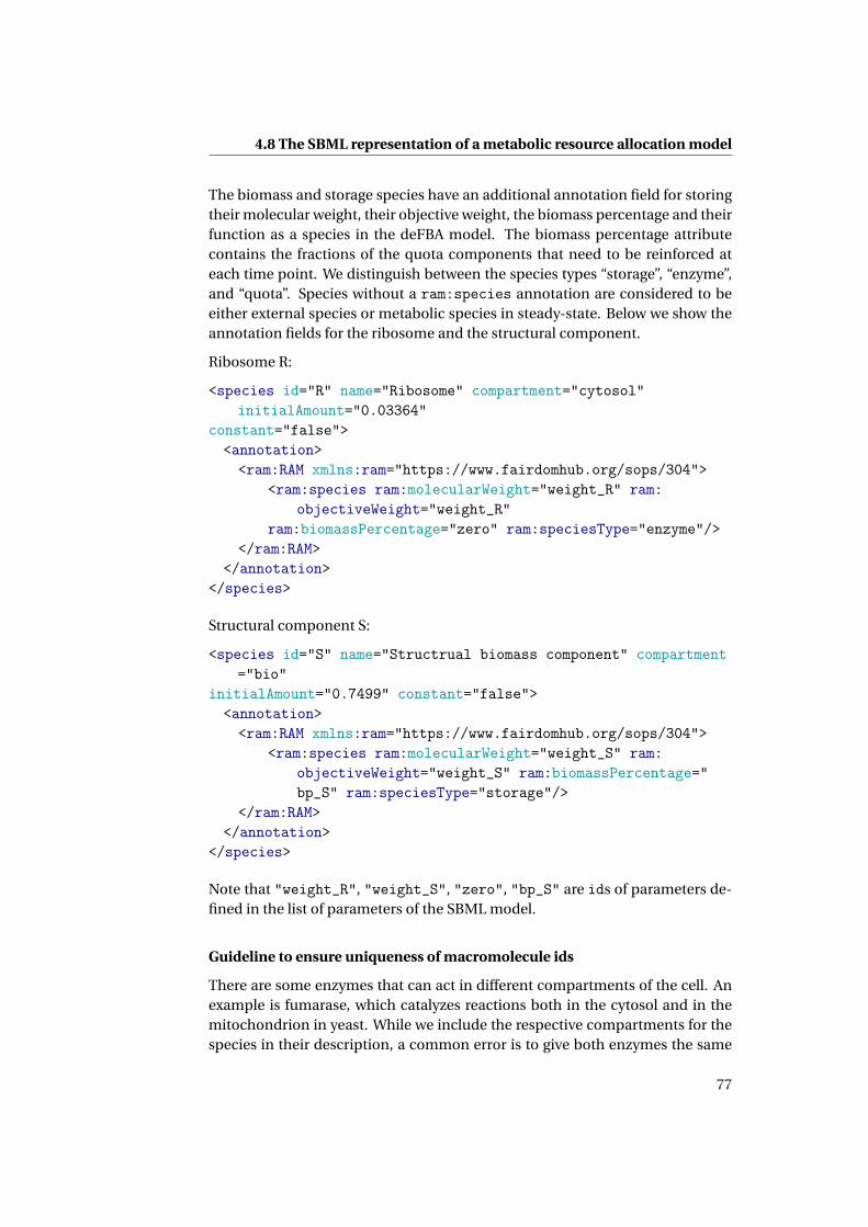
4.8 The SBML representation of a metabolic resource allocation model
The biomass and storage species have an additional annotation field for storingtheir molecular weight, their objective weight, the biomass percentage and theirfunction as a species in the deFBA model. The biomass percentage attributecontains the fractions of the quota components that need to be reinforced ateach time point. We distinguish between the species types “storage”, “enzyme”,and “quota”. Species without a ram:species annotation are considered to beeither external species or metabolic species in steady-state. Below we show theannotation fields for the ribosome and the structural component.
Ribosome R:
<species id="R" name="Ribosome" compartment="cytosol"initialAmount="0.03364"
constant="false"><annotation><ram:RAM xmlns:ram="https://www.fairdomhub.org/sops/304">
<ram:species ram:molecularWeight="weight_R" ram:objectiveWeight="weight_R"
ram:biomassPercentage="zero" ram:speciesType="enzyme"/></ram:RAM>
</annotation></species>
Structural component S:
<species id="S" name="Structrual biomass component" compartment="bio"
initialAmount="0.7499" constant="false"><annotation><ram:RAM xmlns:ram="https://www.fairdomhub.org/sops/304">
<ram:species ram:molecularWeight="weight_S" ram:objectiveWeight="weight_S" ram:biomassPercentage="bp_S" ram:speciesType="storage"/>
</ram:RAM></annotation>
</species>
Note that "weight_R", "weight_S", "zero", "bp_S" are ids of parameters de-fined in the list of parameters of the SBML model.
Guideline to ensure uniqueness of macromolecule ids
There are some enzymes that can act in different compartments of the cell. Anexample is fumarase, which catalyzes reactions both in the cytosol and in themitochondrion in yeast. While we include the respective compartments for thespecies in their description, a common error is to give both enzymes the same
77

Chapter 4. Building and encoding a metabolic resource allocation model
id. Hence, we suggest to name enzymes in a specific pattern combining e.g.their name and their respective location.
If the enzyme is acting in only one compartment we choose its id in the for-mat “Main_id_[acting-compartment]”. If the enzyme is a transporter betweentwo compartments we choose “Main_id_[compartment1]_[compartment2]”. Ifthe enzyme is translated from only one gene (e.g. ETrans1), this represents themain id. For enzyme complexes made of multiple gene products we suggestsimply using “Complex_number” as main id (e.g. Complex_1). Of course, theuser can choose these ids freely, but following these suggestions can help witheasier evaluation of the model in deFBA implementations.
4.8.3 Gene products
Each macromolecule is not only present as a species, but also as a gene prod-uct, with the fields id, label, and associatedSpecies. The id is either thegene name for single gene macromolecules (e.g. ETrans1) or Complex_number(e.g. Complex_1) for complexes as explained above. The label field includesthe recipe for the creation of the enzyme(-complex). The associatedSpeciesis the id of the biomass species associated with this gene product and used forbounding the flux. An example for Complex_1 is:
<fbc:geneProduct fbc:id="Complex_1" label="1*GTRANS1 AND 1*GTRANS2" associatedSpecies="Complex_1"/>
4.8.4 Reactions
All reactions must contain the fields:
• id• reversible (true or false)• fast (true or false)• listOfReactants• listOfProducts
Depending on the kind of reaction, they also include an fbc:geneProductAssociationand a ram:reaction annotation. Additionally, we recommend adding the ECnumber, if known, to the reactions in form of a note:
<notes><body xmlns="http://www.w3.org/1999/xhtml">
<p>EC Number: x.y.z.t</p></body>
</notes>
The id must be unique for each reaction. For reactions producing biomass werecommend starting the id with “synth_” for easier reading and reduced chance
78

4.8 The SBML representation of a metabolic resource allocation model
of assigning the same id multiple times. Furthermore, this makes it easier todistinguish between the reactions from the original metabolic network modeland the deFBA additions. The fast attribute can also be used to distinguishbiomass production reactions (fast = "false") from the rest of the reactions(fast = "true").
The fbc:geneProductAssociation is used to map catalysis relationshipsbetween the enzymes (which are also gene products, see above) and thereactions. Each fbc:geneProductAssociation consists of at most onefbc:geneProductRef, which gives the id of the associated gene product. Reac-tions that do not have a gene product association are considered spontaneous(e.g. the ATP maintenance reaction), and hence their capacity is not boundusing a kcat .
The forward and reverse kcat values for each reaction can be found in the anno-tation, in the fields kcatForward and kcatBackward respectively. It is typicallythe case that the values in the kcatForward and kcatBackward are defined asparameters, and in these fields the ids of the respective parameters are stored,as we will see in the examples below.
The maintenance reaction
As we have seen above, maintenance reactions are typically part of metabolicresource allocation models, since these models do not account for all energy ex-penditures of the cell. The maintenance reactions we consider here are growth-associated, i.e., the flux forced through them is dependent on the total biomassat each time point. Thus, we add an annotation field, maintenanceScaling,which specifies what is the factor f such that
vmaintenance(t ) ≥ f ·biomass(t ).
For typical reactions this field is “zero” as in the case of the metabolic reaction
<reaction id="Metab1_2" reversible="false" fast="true"><annotation><ram:RAM xmlns:ram="https://www.fairdomhub.org/sops/304"><ram:reaction ram:kcatForward="kcat2" ram:kcatBackward="zero
" ram:maintenanceScaling="zero"/></ram:RAM></annotation><fbc:geneProductAssociation fbc:id="Emetab2"><fbc:geneProductRef fbc:geneProduct="Emetab2" />
</fbc:geneProductAssociation><listOfReactants><speciesReference species="N" stoichiometry="1" constant="
true"/>
79

Chapter 4. Building and encoding a metabolic resource allocation model
</listOfReactants><listOfProducts><speciesReference species="AA" stoichiometry="1" constant="
true"/><speciesReference species="ATP" stoichiometry="1" constant="
true"/></listOfProducts>
</reaction>
For the maintenance reaction we have the representation
<reaction id="Maintenance" reversible="false" fast="true"><annotation><ram:RAM xmlns:ram="https://www.fairdomhub.org/sops/304"><ram:reaction ram:kcatForward="zero" ram:kcatBackward="zero"ram:maintenanceScaling="main"/>
</ram:RAM></annotation><listOfReactants><speciesReference species="AA" stoichiometry="50" constant="
true"/><speciesReference species="ATP" stoichiometry="60" constant="
true"/></listOfReactants><listOfProducts></listOfProducts>
</reaction>
4.9 Conclusions
In this chapter we have provided a guide for generating a metabolic resourceallocation model. Together with the step by step guidelines, the links to the rel-evant databases are listed and some guidelines for finding errors that may arisein the model building process are provided. Last but not least, we have pro-posed a standard for exchanging such models using SBML and the flux balanceconstraints package.
We will present in detail in chapters 6 and 7 models that have been generated fol-lowing these guidelines together with the new insights into metabolic resourceallocation we have obtained using them.
However, before we proceed, we dedicate the next chapter to techniques forsolving deFBA problems, numerical concerns, and actual implementation de-tails.
80

Chapter 5
Metabolic resource allocation inpractice: numerical concerns andsolving strategies
Assuming that we have generated a full and correct dynamic resource alloca-tion model following the instructions in the previous chapter, the question thencomes: how do we actually solve this? What discretization scheme do we use?How do we handle numerically the large difference in order of magnitude of theturnover rates and of the enzyme production and metabolic fluxes?
A lot of the work that goes into studying resource allocation is actually spent onprogramming the tools for solving such problems. We discuss in this chapterhow everything was set up and what problems needed to be overcome in orderto obtain the results presented in chapters 6 and 7.
We start by presenting some problems encountered when applying deFBA andcFBA and propose ways to work around these problems. Next, we address nu-merical matters in solving deFBA and cFBA problems and present a reformula-tion of cFBA that alleviates discretization problems. Finally, we offer a concisedescription for the software written to solve deFBA and cFBA problems.
5.1 Artefacts of model formulations
5.1.1 deFBA dependency on the discount factorϕ in the objective
As already mentioned in chapter 2, a practical concern with deFBA is settingthe discount factor ϕ used in the objective function (2.38). Not only do simula-tions depend very strongly on the choice of ϕ as shown in figure 5.1, but there isno way of deciding which value to use for this parameter. Although the deFBAframework itself does not depend on using this particular objective function, we
81

Chapter 5. Metabolic resource allocation in practice: numerical concernsand solving strategies
note that this is the objective used to simulate the fact that the modeled organ-ism has evolved to grow as fast as possible in the given environment. Thus, thisis the objective function used in most applications.
Carbon1,
Carbon1,
Carbon1,
Carbon2,
Carbon2,
Carbon2,
Dext,
Dext,
Dext,
time
exte
rnal m
eta
bolit
e a
mounts
Figure 5.1: External metabolite time courses from the toy deFBA model in (Wald-herr et al., 2015) using ϕ = 0, ϕ = 0.1, and ϕ = 0.3 as objective discount factors.Note that both values 0.1 and 0.3 have been used in the simulations in the deFBAarticle (Waldherr et al., 2015).
The way we have circumvented this problem is simply by eliminating the nega-tive exponential discount altogether (ϕ= 0) and instead using as objective
max∫ t f
0
∑i
bi ni (t )d t , (5.1)
where i denotes a biomass component and the vector b contains the molecularweights of the biomass components.
5.1.2 Linear versus exponential growth in deFBA
Another difficulty arising in solutions of deFBA problems is that, dependingon the extracellular nutrient levels and on the end time t f of the simulation,sometimes a linear growth of the biomass is predicted instead of an exponen-tial growth. In theory, any differentiable function, and hence also the exponen-tial, can be locally approximated by a linear function. We note, however, thatthis behavior is not only observed locally, but over a large portion of the sim-ulation period, corresponding to several consecutive time points spread overseveral hours.
Linear growth is characterized by a linear shape of the total biomass curve overtime. We have noticed this problem arising in three situations:
82

5.1 Artefacts of model formulations
• when the extracellular nutrients run out during the simulation,
• when the simulation end time is too small, and a larger t f would result inexponential growth,
• towards the end of the simulation time a switch from exponential to lineargrowth is sometimes observed.
We believe that this is an artefact of the objective function. As shown in fig-ure 5.2, it takes some time before the linear curve is overtaken by an exponentialcurve, and thus, before this intersection time the linear curve is simply optimalwhile the exponential one is not.
0 2 4 6 8 10time
4
5
6
7
8
9
10
11
12
tota
l bio
mass
Figure 5.2: The total biomass accumulation in the toy model from (Waldherret al., 2015), using an end time t f = 10 (continuous curve) and t f = 60 (dashedcurve). The initial extracellular nutrient amounts are the same as in figure 5.1above. The discount factor has been set as ϕ= 0.
The linear growth results from the system producing only the cheapest biomasscomponent as shown in figure 5.3.
83

Chapter 5. Metabolic resource allocation in practice: numerical concernsand solving strategies
0 2 4 6 8 100
0.2
0.4
0.6
0.8
1
1.2
0 2 4 6 8 100
0.1
0.2
0.3
0.4
0.5
0.6
time time
bio
mass
com
pon
ent
am
ounts
bio
mass
com
pon
ent
am
ounts
Figure 5.3: Time courses of individual biomass components corresponding tofigure 5.2. The left plot shows the time courses for t f = 10 (linear growth), whilethe right plot shows those for t f = 60 (exponential growth).
There is no easy solution to this problem, and we recommend that the modelersimply makes sure that nutrients do not run out during the simulation and that,if a linear growth curve is obtained, then the simulation end time t f should beincreased.
In a starvation scenario, i.e., when the nutrients run out before the end of thesimulation, we observe that deFBA with the biomass integral as objective func-tion (equation (5.1)) predicts linear growth characterized by production of onlythe “cheapest” (in terms of required resources) biomass component. What is ob-served in reality, however, is a much more complex behavior: the cell degradescertain proteins to make other catalytic components from the resulting build-ing blocks in an attempt to survive as long as possible. Simply producing thecheapest component in such a scenario is nothing that would enable the cell tosurvive longer. Therefore, the use of deFBA with the objective (5.1) should bedone with care when modeling a cell in starvation conditions.
5.1.3 deFBA dependency on choice of simulation endpoint
Another issue we found is the dependency of deFBA solutions on the choice ofthe end time t f . We illustrate this in figure 5.4, where the same model has beensimulated using t f = 60 and t f = 150. In this simulation the discounted ob-jective J3 from the original manuscript (Waldherr et al., 2015), correspondingto objective (2.38) in chapter 2, has been used. Thus, as the authors claim, thequantitative differences should not be due to the existence of alternative optima.
84

5.1 Artefacts of model formulations
0 10 20 30 40 50 600
5
10
15
20
25
30Carbon1, t
f=60
Carbon2, tf=60
Dext, tf=60
Carbon1, tf=150
Carbon2, tf=150
Dext, tf=150
exte
rnal m
eta
bolit
e a
mounts
time
Figure 5.4: External metabolite time courses from the original deFBA toy modelin (Waldherr et al., 2015), scenario 1 (carbon switch). The end time points of thesimulations were 60 minutes and 150 minutes. We used one discretization pointper minute and ϕ= 0, which is equivalent to using objective (5.1) above.
As has been already proposed in (Lindhorst et al., 2016), this problem can beovercome by using the short term deFBA (st-deFBA). st-deFBA uses a finite pre-diction horizon and, as the simulations proceed, this moves forward in time.Only the first time point of the result of each simulation is stored as part of thesolution and used as input for the next simulation, where the prediction horizonwindow had moved by one step. The prediction horizon is chosen as the earliestpoint in time at which the exponential strategy leads to a better objective valuethan the linear growth strategy. For the exact details we refer to (Lindhorst et al.,2016). However, using short term deFBA comes at the expense of additional sim-ulation time since at each step in the solution a new LP is solved.
We have considered in the work presented here that the end time dependency issmall enough to be neglected and have used deFBA as in (Waldherr et al., 2015).
Obviously, one can argue that this end time point dependency does not exist incFBA. However, cFBA is only suited for organisms displaying balanced growthin a periodic environment such as cyanobacteria or algae. For other organisms,like yeast, there is no reason why we should have periodic biomass compositionconstraints.
cFBA comes however, with a different difficulty related to optimality as we willsee in section 5.5.
85

Chapter 5. Metabolic resource allocation in practice: numerical concernsand solving strategies
5.2 Numerical considerations and scaling
5.2.1 The midpoint rule discretization
To numerically solve deFBA and cFBA problems, the dynamic variables for themacromolecule and external metabolite amounts need to be discretized in time.The authors of deFBA propose a Gauß-Legendre method with Radau colloca-tion points of order 2 and 3 using a Lagrange polynomial interpolation function,while the authors of cFBA use an iterative scheme that turns out to be mathe-matically equivalent to the simplest discretization method, explicit Euler.
The explicit Euler method can be shown to be numerically unstable, in partic-ular for stiff equations. This means that the numerical solution obtained usingexplicit Euler becomes very large for equations where the exact solution doesnot. This is the reason why this numerical method should not be used in prac-tice. On the other hand, a Gauß-Legendre method with Radau collocation pointsof order 2 and 3 using a Lagrange polynomial interpolation function is not onlydifficult to implement, but it also susceptible to interpolation errors known asRunge’s phenomenon. These are oscillations that appear at the edges of the in-terpolation interval when using identically spaced interpolation points (Runge,1901).
A much simpler and stable choice is to use the implicit midpoint rule, which isthe simplest collocation method (after the Euler schemes). In short, this statesthat, given a differential equation
y ′(t ) = f (t , y(t )),
and a step size h, we can discretize it as
yk = yk−1 +h · f
(tk−1 +
h
2,
yk + yk−1
2
),
where yk is the numerical solution at time point tk .
This method allows us to preserve a simple implementation and, at the sametime, guarantees numerical stability even for stiff equations. Therefore, we havedecided to use the implicit midpoint rule in the studies presented in chapters 6and 7.
Specifically, fixing a number of discretization points N = t f
h , we discretize thedynamic variables for macromolecule and extracellular metabolite amount (n)at each discretization point tk , while the fluxes v and the derivative values nare evaluated always in the middle of the discretization intervals at tk+tk−1
2 . This
86

5.2 Numerical considerations and scaling
means that for the dynamic optimization problem in section 2.3.5 we obtain:
maxn,n,v
N∑k=1
∑i∈{L,M ,T,R,Q}
ni (tk ) (5.2)
s.t. nSout
(tk + tk−1
2
)=−vT
(tk + tk−1
2
)(5.3)
0 = vT
(tk + tk−1
2
)−vM
(tk + tk−1
2
)(5.4)
0 = vM
(tk + tk−1
2
)−vL
(tk + tk−1
2
)− ∑
i∈{L,M ,R,T }vRi
(tk + tk−1
2
)(5.5)
nQ
(tk + tk−1
2
)= vL
(tk + tk−1
2
)(5.6)
ni
(tk + tk−1
2
)= vRi
(tk + tk−1
2
), ∀i ∈ {L, M ,T,R} (5.7)
vi
(tk + tk−1
2
)≤ k i
catni (tk )+ni (tk−1)
2, ∀i ∈ {L, M ,T } (5.8)
∑i∈{T,L,M ,R}
vRi
( tk+tk−12
)kRi
cat
≤ nR (tk )+nR (tk−1)
2(5.9)
n(tk ),v(
tk + tk−1
2
)≥ 0 (5.10)
nQ (tk ) ≥ q∑
i∈{L,M ,T,R,Q}ni (tk ) (5.11)
n(tk ) = ntk−1 +hn(
tk + tk−1
2
), (5.12)
for all k ∈ {1, . . . , N }.
This practically means that the LP problem has, for each macromolecule 2Ndifferent variables (N concentration and N derivative variables) and for eachreaction flux N different variables related using the constraints above.
5.2.2 Cyclicity and discretization problems
In this section we point out that also the midpoint rule can lead to strong numer-ical errors. This can in particular be seen in the case of using a cyclic objectiveand maximizing the multiplication factor α as done in cFBA. The following ex-ample illustrates this. Assume we are looking at a system with only one reaction
X → P,
which has flux v and the reaction is catalyzed by P with a turnover rate kcat .Then we want to find the maximum multiplication factor α as follows:
87

Chapter 5. Metabolic resource allocation in practice: numerical concernsand solving strategies
maxv,nP
α
s.t. nP = v
v ≤ kcat nP
nP (t f ) =αnP (0)
We take the simplest case and use only one time step in the discretization, thelength of which is t f . That means that the derivative nP and the flux v are con-stant, and the expression for nP (t f ) is given by
nP (t f ) = nP (0)+ t f nP (5.13)
and the capacity bound for v becomes
v ≤ kcatnP (t f )+nP (0)
2,
since in the midpoint rule we evaluate nP in the middle of the time interval [0, t f ]
and approximate the lacking value of nP
(t f
2
)by
nP (t f )+nP (0)2 .
To get the largest multiplication factor α, it is obvious that a flux v will be cho-sen such that the flux capacity constraint v ≤ kcat nP is satisfied with equality,therefore
v = kcatnP (t f )+nP (0)
2.
Replacing nP (t f ) by means of equation (5.13), we get
v = kcatnP (0)+ t f nP +nP (0)
2= kcat
(nP (0)+ t f
2nP
).
Since nP = v , we have
v = kcat
(nP (0)+ t f
2v
)⇔ v = kcat nP (0)
1−kcatt f
2
.
Substituting back in equation (5.13), we get
nP (t f ) = nP (0)+ t fkcat nP (0)
1−kcatt f
2
,
and from the cyclicity constraint then
nP (t f ) = nP (0)+ t fkcat nP (0)
1−kcatt f
2
=αnP (0).
88

5.2 Numerical considerations and scaling
From the last equation we can then obtain the multiplication factor α as
α= 1+ t fkcat
1−kcatt f
2
, (5.14)
which points out that α depends on the end point of the simulation t f . In par-
ticular, the multiplication factor becomes infinite as kcatt f
2 approaches 1, that iswhen the time step approaches 2
kcat.
This points out an unintuitive effect of the combination between the differentialequation discretization and the cyclicity of the system. We believe that this isnot restricted to cyclic problems, but is a general issue of deFBA and cFBA. Inthe cyclic case it is only particularly easy to exhibit the artefact. In the followingsection we show how one can avoid this problem by reformulating the problemand introducing a dilution term in the differential equation for nP .
5.2.3 cFBA with dilution term
Problem reformulation
We start with a model
nE (t ) = SE∗v(t ) ∀t ≥ 0
0 = SM∗v(t ) ∀t ≥ 0
Av(t ) ≤ BnE (t ) ∀t ≥ 0
αnE (0) = nE (t f ),
where SE∗ are the enzyme-producing stoichiometries and SM∗ describes themetabolism. A,B can be arbitrary matrices to constrain fluxes by enzymeamounts.
With a slight abuse of notation, for arbitrary µ > 0 we define the enzyme con-centrations e and fluxes w subject to dilution by µ as
e(t ) := nE (t )
V (0)exp(µt )
w(t ) := v(t )
V (0)exp(µt ),
where V (0) is the initial volume of the cell population.
89

Chapter 5. Metabolic resource allocation in practice: numerical concernsand solving strategies
This yields
e(t ) = d
d t
nE (t )
V (0)exp(µt )= nE (t )
V (0)exp(µt )−µ nE (t )
V (0)exp(µt )
⇒ e(t ) = SE∗v(t )
V (0)exp(µt )−µe(t )
⇒ e(t ) = SE∗w(t )−µe(t )
0 = SM∗w(t )
Aw(t ) ≤ Be(t )
αe(0)V (0) =V (0)exp(µt f )e(t f )
Hence, with α= exp(µ · t f ), we get e(0) = e(t f ).
This way we can transform a cFBA problem formulation into a formulation thatincludes dilution by growth. By doing the transformation backwards, we cantransform a steady-state solution of the dilution model (e,w variables) to a uni-form growth solution of the original problem (n, v variables).
Note that bounds on concentrations and fluxes are still possible. Moreover, it iseven possible that the constraint matrices A and B depend on time.
Discretization error in the dilution formulationThe dilution formulation of the problem is no longer affected by the discretiza-tion errors described in the previous section. To see this, we consider again theexample in section 5.2.2, where we are looking at a system with only one reaction
X → P,
which has flux w and the reaction is catalyzed by P with a turnover rate kcat . Inthe transformed problem formulation we want to find the maximumµ using thefollowing optimization problem:
maxµ
s.t. eP = w −µeP (5.15)
w ≤ kcat eP (5.16)
eP (0) = eP (t f ) (5.17)
We consider again the simplest case, using one time step of length t f for dis-cretization. This means that, by applying the discretization, we obtain
eP (t f ) = eP (0)+ t f · eP(5.17)⇔ eP (0) = eP (0)+ t f · eP ⇔ eP = 0. (5.18)
The bound (5.16) is applied taking the midpoint rule into account, as in sec-tion 5.2.2, using the value of eP at the middle of the time interval, i.e.,
w ≤ kcateP (0)+eP (t f )
2
(5.17)⇔ w ≤ kcat eP (0).
90

5.3 Connections between cFBA and RBA
To get the largest µ, it is obvious that w will be chosen such that constraint (5.16)is satisfied with equality and we thus obtain
w = kcat eP (0). (5.19)
From equations (5.15), (5.18), and (5.19), we observe that
w =µeP (0) and w = kcat eP (0),
which shows thatµ= kcat .
We thus observe that the expression for µ no longer depends on the end time t f
as it did in (5.14). Moreover, we observe that, with
α= exp(µ · t f ) ⇔µ= log(α)
t f,
the values for µ and α are compatible when taking the limit t f → 0 in equa-tion (5.14),
limt f →0
log(α)
t f
(5.14)= limt f →0
log
(1+ t f
kcat
1−kcatt f2
)t f
l′Hôpital= limt f →0
11+t f
kcat
1−kcatt f2
· kcat
(1−kcat
t f2
)+t f
kcat2
2(1−kcat
t f2
)2
1
= kcat .
ConclusionIt is not coincidental that we have chosen µ for the transformation. µ is theactual growth rate of the exponentially growing system.
To keep the simplicity of explanations in chapter 6, we consider this dilutiontransformation an implementation detail. We still describe the model using theoriginal cFBA formulation, although in the solving software we implement thedilution formulation.
5.3 Connections between cFBA and RBA
After the dilution transformation, we observe that the cFBA problem formula-tion looks strikingly similar to RBA, and that cFBA with one time step is in factequivalent to RBA. Indeed, we show in this section that RBA provides an upperbound on growth rates obtained using cFBA.
91

Chapter 5. Metabolic resource allocation in practice: numerical concernsand solving strategies
We recall from chapter 2 that concentration is defined as the number ofmolecules n of substance present in a certain volume V of a solution, i.e.,c(t ) = n(t )
V (t ) . While in section 3.2 we assumed a constant volume, we now allowthe volume to change over time. This happens for example in the case of cellgrowth, when the total volume of all cells grows.
The metabolic network usually consumes and produces metabolites as speci-fied in the stoichiometric matrix S. The product SM∗v(t ) then gives the changein metabolite concentrations when the volume stays constant. This product re-flects the net production of each metabolite by the metabolic network. In casethe volume changes, we also obtain a dilution term, as in RBA and as in sec-tion 5.2.3 above, so
c(t ) = SM∗v(t )−µ(t )c(t ), (KM2a)
e(t ) = SE∗v(t )−µ(t )e(t ),
where the growth rate µ(t ) is defined as
µ(t ) := V (t )
V (t ). (5.20)
We observe that
µ(T ) := 1
T
∫ T
0µ(t )d t . (AVGM)
is the average growth rate:
Proposition 5.3.1 It holds for all T ≥ 0 that V (T ) =V (0)exp(µ(T )T ).
PROOF We define W (t ) := ln(V (t )) for all t ≥ 0. It follows that
W (t ) = V (t )
V (t )=µ(t ) (5.21)
⇒∫ T
0µ(t )d t =
∫ T
0W (t )d t =W (T )−W (0) (5.22)
⇒ V (T )
V (0)= exp(W (T )−W (0)) = exp
(∫ T
0µ(t )d t
). (5.23)
The proposition follows by definition of µ. ■
5.3.1 Modeling assumptions (with dilution)
For ease of notation, we use z := (c,e)ᵀ and treat enzyme and metabolite concen-trations together in the results we derive here. Following the derivation abovebased on (KM2a), we now consider the new kinetic model
z(t ) = Sv(t )−µ(t )z(t ), (KM2)
v(t ) = f (z(t )),
92

5.3 Connections between cFBA and RBA
where f denotes the kinetic rate law functions. The system (KM2) now alsomodels dilution of internal metabolites and enzymes via cell growth. The restof the assumptions are the same as in section 3.2.1. In addition we assume thatthe growth rateµ(t ) is positive, bounded and continuous for all time points t ≥ 0.
5.3.2 Average fluxes and average concentrations
For a given time period T , we additionally define the average concentrations zas:
z(T ) := 1
T
∫ T
0
µ(t )
µ(T )z(t )d t . (AVGZ)
Note that we scale the concentrations by the growth rate µ. The motivationfor this is that, in order to avoid depletion of metabolite pools, it is muchmore important to overproduce metabolites in fast-growing periods than inslow-growing ones. We observe that z(T ) can be considered an average overgrowth rates rather than over time since
z(T ) =∫ T
0 µ(t )z(t )d t∫ T0 µ(t )d t
. (5.24)
As in the case for the average fluxes v, it can happen that
z := limT→∞
z(T ), (5.25)
µ := limT→∞
µ(T ) (5.26)
do not exist. Hence we again assume, for simplicity, that the limits v, z, and µ
exist and refer the reader to the appendix of (Reimers and Reimers, 2016) for thecase where they do not exist.
We observe in the following that, if we consider dilution, the steady-state condi-tion for the average fluxes changes slightly:
Theorem 5.3.2 Sv = zµ.
PROOF Following the same arguments as in the proof of theorem 3.2.1, we ob-tain that
limT→∞
1
T
∫ T
0Sv(t )−µ(t )z(t )d t = 0. (5.27)
We can then use equations (AVGV), (5.24), and (AVGM) to arrive at the theorem
93

Chapter 5. Metabolic resource allocation in practice: numerical concernsand solving strategies
statement as
0 = limT→∞
1
T
∫ T
0Sv(t )d t − lim
T→∞1
T
∫ T
0µ(t )z(t )d t (5.28)
(AVGV)= Sv− limT→∞
1
T
∫ T
0µ(t )z(t )d t (5.29)
(5.24)= Sv− limT→∞
z(T )1
T
∫ T
0µ(t )d t (5.30)
(AVGM)= Sv− zµ. (5.31)■
One way to understand theorem 5.3.2 is to think of z as the composition of thebiomass of an RBA model. µ is then the flux through the biomass productionreactions. Because z includes in our case all macromolecules and all metabolitespresent in the cell, all these have to be duplicated upon cellular division. Thisway, the dilution term enforces the production of all macromolecules present inthe cell.
We observe here a shortcoming in the formulation of RBA and cFBA, which ig-nore metabolite dilution by growth. We check the impact of this shortcoming inthe next section.
5.3.3 Violation of the steady-state condition by dilution
In the following we estimate the order of magnitude of this violation relative tothe fluxes. For this purpose let us assume that the RBA model approximates zwith a total error of 1 mM. We again use the three organisms Escherichia coli,Saccharomyces cerevisiae and Homo sapiens as examples. The detailed calcu-lations for the three organisms are presented in Appendix A. Other exampleswhere the same trend can be observed can be found in (Stephanopoulos et al.,1998).
Escherichia coli
E. coli has an average cell volume of 0.6 µm3 (Kubitschek, 1990), a dry weight of0.489 pg (Loferer-Krößbacher et al., 1998), an average growth rate on glucose of0.9 h−1 (Andersen and von Meyenburg, 1980), and a glucose uptake rate of 12mmol/(gDW ·h) (Jain and Srivastava, 2009). Using these values it follows that anapproximation error of 1 mM for z implies a violation of the steady-state condi-tion in the order of 10−4 relative to the fluxes.
Saccharomyces cerevisiae
A similar result is obtained in the case of S. cerevisiae, which has an averagegrowth rate on glucose of 0.4 h−1 (Waldron and Lacroute, 1975), average intra-
94

5.3 Connections between cFBA and RBA
cellular fluxes of 0.5 mmol/(gDW ·h) (Stewart et al., 2010), a dry weight of ap-proximately 10−11 g = 10 pg (Mitchison, 1958), and a volume of 20 µm3 (Tysonet al., 1979). These values imply that an approximation error of 1 mM for z leadsto a violation of the steady-state condition in the order of 10−3 relative to thefluxes.
Homo sapiens (HeLa cells)
In the case of HeLa cells we obtain a similar order of magnitude for the violation.HeLa cells have an average growth rate of 0.06 h−1 (Kumei et al., 1989), glucoseuptake flux of about 18 nmol/(min ·mg protein) (Mojena et al., 1985), approxi-mately 150 pg protein (Finka and Goloubinoff, 2013), and a volume of 2600 µm3
(Luciani et al., 2001; Finka and Goloubinoff, 2013). With these values, an ap-proximation error of 1 mM for z implies a steady-state condition violation in theorder of 10−3 relative to the fluxes.
5.3.4 Bounds for cFBA from RBA
Let µ∗ be the optimum of the following optimal control problem formulatedbased on the kinetic model (KM2):
µ∗ := maxv(t ),z(t ),µ
µ
s.t. z(t ) = Sv(t )−µ(t )z(t ) ∀t ≥ 0
−K −z(t ) ≤ v(t ) ≤ K +z(t ) ∀t ≥ 0 (OCP2)
l(t ) ≤ v(t ) ≤ u(t ) ∀t ≥ 0,
where l(t ) and u(t ) are time-dependent functions that can be used to enforcelimits from the environment, and K −,K + are matrices containing the turnoverrates for the forward and reverse directions of the reactions.
Let µ∗RBA denote the optimum of the following RBA problem:
µ∗RBA := max
v,z,µµ
s.t. Sv = zµ (RBA2)
−K −z ≤ v ≤ K +z
l ≤ v ≤ u,
where l, u are defined as
l := limT→∞
1
T
∫ T
0l(t )d t ,
u := limT→∞
1
T
∫ T
0u(t )d t ,
assuming the limits exist.
95

Chapter 5. Metabolic resource allocation in practice: numerical concernsand solving strategies
In this case it also holds that the RBA optimum gives an upper bound for thegrowth rate µ∗:
Corollary 5.3.3 It holds that µ∗RBA ≥ µ∗.
PROOF Assume the limits v and z exist. Then, by theorem 5.3.2, Sv = zµ.
Since µ does not change over time in (OCP2), it follows that
µ(T ) =µ
and thus we have
z = limT→∞
1
T
∫ T
0z(t )d t .
By the linearity of the enzyme capacity constraint in (OCP2), we obtain
−K − limT→∞
1
T
∫ T
0z(t )d t ≤ lim
T→∞1
T
∫ T
0v(t )d t ≤ K + lim
T→∞1
T
∫ T
0z(t )d t ,
which is equivalent to−K −z ≤ v ≤ K +z.
It is also easy to see that v satisfies l ≤ v ≤ u. Thus, we observe that v, z,µ is afeasible solution of (RBA2).
If v and z do not exist, we instead can use theorem 3 in Appendix A of (Reimersand Reimers, 2016) and any accumulation point pair v, z will be a feasible solu-tion of RBA2. ■
Since cFBA assumes a constant growth rate over the whole cycle, similar to(OCP2), we therefore conclude that RBA provides upper bounds on growthrates from cFBA models. This fact can conveniently be used when debuggingimplementation errors of dynamic resource allocation models as described inchapter 4.
5.4 Condition numbers, time scale separation and scaling
To derive the quasi-steady-state approximation, the inventors of deFBA makeuse of a transformation that reflects the fact that macromolecule production re-actions are much slower than metabolic reactions and that the macromoleculeamounts in general change much more slowly than metabolite amounts. Thistransformation effectively means that the macromolecule production fluxes arescaled by a small dimensionless factor ε.
This transformation also has practical consequences for the solving imple-mentation. Since macromolecule production fluxes are much smaller thanmetabolic fluxes, we obtain a large order of magnitude difference between thesevariables inside the LP. This large difference gives rise in general to numerical
96

5.4 Condition numbers, time scale separation and scaling
inaccuracies and rounding errors, as explained in (Klotz, 2014). By scaling themacromolecule production fluxes, the macromolecule concentrations and theirderivatives, we thus avoid such rounding errors. For ease of notation, we alsoconsider this an implementation detail and do not include it in the problemdescriptions in this thesis, but only in the software implementation.
Despite the ε scaling, additional numerical inaccuracies can stem from the kcat
values used. A quick look at figure 4.2 will reveal that these parameters spreadover several orders of magnitude. The only kind of scaling that can help improvethe numerical stability in this case is the individual scaling of problematic rowsof the constraint matrices.
To get an intuition about the numerical condition of typical dynamic metabolicresource allocation problems, we compute the condition number of the basismatrices corresponding to typical solutions of the problems in chapters 6 and 7.
5.4.1 Recap on matrix condition numbers
Let us first have a look at the derivation of the condition number, which we haveadapted from (Klotz, 2014). Given the linear programming problem
max aT x (5.32)
s.t.Ax = b (5.33)
x ≥ 0, (5.34)
we look at the subset B of the rows of the matrix A that is present in the basis.The solution at this point is thus given by
xB = A−1B∗b.
Considering a small perturbation∆b of the right hand side b, we are interested inthe change ∆xB this perturbation will induce in the solution xB . After a coupleof computations and after applying the Cauchy-Schwarz inequality, we obtainthe upper bound
||∆xB || ≤ ||A−1B∗|| · ||∆b||. (5.35)
Similarly,
||b|| ≤ ||AB∗|| · ||xB ||. (5.36)
Multiplying the left and right hand sides of (5.35) and (5.36) together and rear-ranging terms we obtain
||∆xB ||||xB ||
≤ ||AB∗|| · ||A−1B∗||
( ||∆b||||b||
),
97

Chapter 5. Metabolic resource allocation in practice: numerical concernsand solving strategies
which gives an upper bound on the relative change in the solution upon theperturbation ||∆b||. For more details of the derivation we refer to (Klotz, 2014).
We observe that the condition number of the basis matrix, which is a submatrixof the constraint matrix A, defined as
κ(AB∗) = ||AB∗|| · ||A−1B∗||
is a factor in the upper bound on the error we obtain upon a perturbation. Thisnumber is a property of the modeled system rather than a result of roundingerrors. Since ill-conditioning of a problem is typically defined as a small per-turbation in the input giving rise to a large error in the output, the conditionnumber allows us to assess the ill-conditioning of a problem given (submatricesof) its constraint matrix A.
The rounding errors that occur in finite precision computing environments canalso be seen as perturbations to the entries of the constraint matrix or the righthand side. These errors can be increased by a large condition number. To givean intuition, assume ||∆b|| is in the order of 10−16 and κ(AB∗) is in the order of1013. Then rounding errors up to 10−16 ·1013 = 10−3 can arise in the calculations.In such cases, algorithms of LP solvers can run into numerical difficulties.
5.4.2 Condition numbers for typical deFBA and cFBA problems
The basis matrix of a typical solution of the Synechococcus elongatus model inchapter 6 has a condition number in the order of 1011, while that of a typical so-lution of the Saccharomyces cerevisiae model in chapter 7 has a condition num-ber in the order of 109. Note that these condition numbers are obtained after thescaling by ε explained above.
In the light of the example above, these values are obviously large enough topresent a problem for standard commercial solvers such as CPLEX or Gurobi,which offer feasibility check precision of only up to 10−9.
Therefore, to minimize the potential rounding errors appearing, we havedecided to use an open source LP solver, SoPlex (Wunderling, 1996; Gleixneret al., 2012, 2016), with higher precision (up to 10−16) than standard commercialsolvers, and which can perform iterative refinement of the solution, going up toarbitrary precision.
This increase in precision comes however at the expense of increased solvingtime. In addition, the solving time is further increased in the software writtenfor this thesis by the lack of an interface of SoPlex for MATLAB. This results ineach LP having to be written to file by the MATLAB code and then read by thesolver. With large LPs such as those resulting from dynamic resource allocationproblem, this becomes a real challenge.
98

5.5 Convexity of the binary search in cFBA
5.5 Convexity of the binary search in cFBAWhile deFBA problems become linear programs after the discretization andhence are guaranteed to arrive at a global optimum, this is not the case for cFBAproblems because of the quadratic terms in the constraints.
Similar to RBA and ME models, cFBA uses a binary search procedure to arrive atthe optimal multiplication factor α+ which corresponds to the optimal growthrate µ+. However, we need to prove mathematically that this binary search isguaranteed to arrive at the optimal growth rate. To prove this, one has to showthat, if the organism can grow at a growth rate µ+, then it can also grow at anygrowth rate µ ∈ [0,µ+]. While biologically this is intuitively correct, we also showhere how it works out mathematically.
We can only prove the convexity of a slightly modified problem, where weweaken the constraint
e(t ) = SE∗w(t )−µ+e(t )
by only requiring an inequality, as
e(t ) ≤ SE∗w(t )−µ+e(t ).
At a steady-state, as in the case of RBA, this would mean that production ofmacromolecules has to be greater or equal to dilution by growth, i.e.,
SE∗w(t )−µ+e(t ) ≥ 0,
which is the same as constraint (2.14) in the RBA formulation.
Theorem 5.5.1 Given a feasible solution(w(t )+,e(t )+,µ+)ᵀ with µ+ > 0 of the
optimization problem
maxw(t ),e(t ),µ
µ
s.t. e(t ) ≤ SE∗w(t )−µe(t )
0 = SM∗w(t ) (OCP3)
Aw(t ) ≤ Be(t )
e(0) = e(t f )
for everyµ≥ 0,δµ> 0 withµ+ =µ+δµ,(w(t )+,e(t )+,µ
)ᵀ is also a feasible solutionof (OCP3).
PROOF Sincee(t )+ ≤ SE∗w(t )+−µ+e(t )+
is the only constraint where µ+ appears, we only need to check that this is satis-fied also for the smaller growth rate µ. With µ+ =µ+δµ, for δµ> 0, we obtain
e(t )+ ≤ SE∗w(t )+− (µ+δµ)e(t )+ ≤ SE∗w(t )+−µe(t )+,
since the term δµ ·e(t )+ is positive. ■
99

Chapter 5. Metabolic resource allocation in practice: numerical concernsand solving strategies
From a biological perspective, weakening the constraint as above is equivalentto overproducing amino acids or energy, and most organisms have mechanismsto dissipate excess energy such as futile cycles or wastage of ATP by an ATPase.However, by weakening the constraint for the cyanobacterium model in chap-ter 6, we obtain a slightly increased growth rate in the reference day case (3.68%increase in µ). This points out that indeed using the equality version is a restric-tion to the system and this may be one reason why we were not able to prove astronger convexity statement.
5.6 Implementation
In this section we give a very brief description about implementing deFBA (andits cFBA variant) and what are necessary parts of this implementation. For anexample implementation focused on deFBA we refer the reader to the githubrepository at https://github.com/alexandra-m-reimers/deFBA.
5.6.1 Variables
The variables of a deFBA problem are the fluxes v, the amounts for the extra-cellular metabolites and macromolecules n, and their derivatives n. Each ofthese variables in turn has N instances, one for each time point of the discretiza-tion. We can therefore imagine v for instance as a matrix with N rows and |R|columns. The same then applies for n and n. Therefore, a deFBA numericalsolution is a structure made of these three different matrices. At this point it isclear that a necessary ingredient of the implementation are two functions thatcan convert from the solution vector to the variable matrices (toStruct) and back(toVector) for ease of access of the results as well as for easily formulating theconstraints.
In addition to v, n, n, if one does not want to split reversible reactions, thenhelper variables for imposing the capacity bounds are needed. As an example,assume reversible reaction r1 and irreversible reaction r2 are both catalyzed byenzyme e1, with turnover rates k1 and k2 respectively. Then the capacity boundfor them is given by
|vr1 (t )|k1
+ vr2 (t )
k2≤ ne1 (t ).
Obviously, we need to reformulate this constraint since LP solvers cannot han-dle absolute values. One way to do this, is to introduce helper variables E and
100

5.6 Implementation
formulate this constraint as
vr1 (t ) ≤ k1Er1 (t )
−vr1 (t ) ≤ k1 ·Er1 (t )
vr2 (t ) ≤ k2Er2 (t )
Er1 (t )+Er2 (t ) ≤ ne1 (t )
E(t ) ≥ 0
This formulation allows us the flexibility of also having different turnover ratesfor the forward and the reverse direction of a reaction. E has the same structureand dimensions as the vector v.
However, another special case to be handled is also the case where another en-zyme e2 catalyzes r2 and another reaction r3. We already notice that we wouldneed a second, different Er2 (t ) variable for implementing this constraint as ex-plained above. Therefore, we need to look at E as a three dimensional matrix,with one dimension for the reactions, one for the enzymes, and one for the timepoints. We therefore talk for example about variables like Ee1
r1(t ). At this point it
becomes even more clear that the functions toStruct and toVector are crucial foravoiding implementation mistakes.
5.6.2 Constraint matrix
The constraint matrix of a deFBA (or cFBA) problem contains several constrainttypes:
• differential equations equality constraint for external metabolites (e.g.(5.3)) and macromolecules (e.g. (5.6)-(5.7))
• steady-state equality constraint for internal metabolites (e.g. (5.4)-(5.5))
• enzyme capacity inequality constraint (e.g. (5.8)-(5.9))
• discretization equality constraint for relating n to n (e.g. (5.12))
• inequality constraint to impose quota macromolecule production (e.g.(5.11)).
For ease of implementation and debugging, we recommend that a function iswritten for constructing the submatrix of the constraint matrix and the subvec-tor of the right hand side corresponding to each type of constraint. Then thesesubmatrices and subvectors can be merged and passed to the solver. In a similarfashion, a function should be written to build the objective vector.
To build all these constraint submatrices, a key element is a function that, givena variable type (e.g. v), the reaction (resp. component) index, and the time pointreturns the index of this variable in the solution vector (getIndex).
101

Chapter 5. Metabolic resource allocation in practice: numerical concernsand solving strategies
5.6.3 Bounds on variables
Using the function getIndex, positivity constraints and bounds on irreversible orexchange reactions can be formulated for each time point. In a similar fashion,dynamic bounds as the light uptake in chapter 6 can be formulated.
5.6.4 Shift experiments
In case one wants to perform nutrient shift experiments as in chapter 7, someof the constraints need to be adjusted. For example, assume that at time point 3one nutrient source y1 is removed. Obviously, the constraint
ny1 (3) = ny1 (2)+h · ny1 (2.5)
no longer holds. In such cases, this discretization constraint needs to be re-moved. In addition, the constraint that lby1 (3) = uby1 (3) = 0 needs to be added,where lb, ub are the lower and upper bound vectors of the LP.
The best way to implement such constraints is to have a structure as part ofthe model that stores the variable type (n in this case), the index of the shiftedcompound (index of y1) and the time point at which the shift occurs (3 in thiscase). This structure then has one field for each shift.
Shifts in nonlimiting extracellular metabolites (e.g. O2 in yeast), for which we donot model an explicit amount but instead the amount taken up is only boundedby the turnover rate and the transporter amount, are easier to implement sincewe do not need to drop any constraint, but only impose flux bounds at the re-spective time points.
5.6.5 Short term deFBA
In case one wants to implement the short term deFBA (Lindhorst et al., 2016),which we have introduced briefly in section 5.1.3, a loop around a typical deFBArun is sufficient. At each step of the loop a deFBA problem is solved over thegiven prediction horizon (t f ) and the values of the first time point of the solutionare stored and passed on as initial values to the next iteration. A way of findingthe minimum prediction horizon such that exponential growth is preferred tolinear growth (cf. section 5.1.2) is described in (Lindhorst et al., 2016).
In case shift experiments are implemented, with each iteration the shift timepoint comes “closer” and the time point values for the shifts need to be updatedalso.
102

Chapter 6
Cellular tradeoffs and optimalresource allocation duringcyanobacterial diurnal growth
The work presented in this chapter has been done in collaboration withHenning Knoop and Ralf Steuer. This work has been published in Pro-ceedings of the National Academy of Sciences (PNAS) under (Reimerset al., 2017a) and can be found at http://dx.doi.org/10.1073/pnas.1617508114.
Cyanobacteria are an integral part of the Earth’s biogeochemical cycles anda promising resource for the synthesis of renewable bioproducts from atmo-spheric CO2. Growth and metabolism of cyanobacteria are tied to the diurnalrhythm of light availability. So far, however, insight into the stoichiometricand energetic constraints of cyanobacterial diurnal growth is limited. In thischapter we investigate the optimal allocation of cellular resources duringdiurnal phototrophic growth using a genome-scale metabolic reconstructionof the cyanobacterium Synechococcus elongatus PCC 7942. We formulatephototrophic growth as an autocatalytic process and solve the resulting time-dependent resource allocation problem using cFBA. Based on a narrow andwell-defined set of parameters, we obtain an ab initio prediction of growthproperties over a full diurnal cycle. The computational model allows us tostudy the optimality of metabolite partitioning during diurnal growth. Thecyclic pattern of glycogen accumulation, an emergent property of the model,has timing characteristics that are in qualitative agreement with experimentalfindings. Our model gives insight into the dynamic resource allocation problemof phototrophic diurnal growth. Furthermore, it serves as a general framework
103

Chapter 6. Cellular tradeoffs and optimal resource allocation duringcyanobacterial diurnal growth
to assess the optimality of metabolic strategies that evolved in phototrophicorganisms under day-night conditions.
6.1 Introduction
Cyanobacterial photoautotrophic growth requires a highly coordinated distri-bution of cellular resources to different intracellular processes, including the denovo synthesis of proteins, ribosomes, lipids, and other cellular components.For unicellular organisms, the optimal allocation of limiting resources is a keydeterminant of evolutionary fitness. The protein economy and its implicationsfor bacterial growth laws have been studied extensively. However, this was donealmost exclusively for heterotrophic organisms under stationary environmen-tal conditions (Molenaar et al., 2009; Scott et al., 2010; Flamholz et al., 2013;Vázquez-Laslop and Mankin, 2014; Hui et al., 2015; Burnap, 2015; Weiße et al.,2015).
For photoautotrophic organisms, including cyanobacteria, growth-dependentresource allocation is further subject to light-dark cycles that partition cellu-lar metabolism into distinct phases. Recent experimental results have demon-strated the relevance of time-specific synthesis for cellular survival and growth(Shultzaberger et al., 2015; Diamond et al., 2015; Lambert et al., 2016). Nonethe-less, the consequences of a day-night environment on the cellular resource al-location problem are insufficiently understood, and computational approachesdeveloped for heterotrophic organisms are not straightforwardly applicable todiurnal phototrophic growth (Westermark and Steuer, 2016).
Here, we use dynamic optimization to study optimal diurnal resource allocationfor phototrophic growth. We are mainly interested in the stoichiometric andenergetic constraints that shape the relationship between the maximal growthrate and the relative partitioning of metabolic, photosynthetic, and ribosomalproteins during a full day-night cycle. We aim to obtain a prediction of the prop-erties that arise from a narrow and well-defined set of parameters and assump-tions about cyanobacterial growth – and to contrast these properties with exper-imentally observed behavior.
We assemble and numerically evaluate an autocatalytic genome-scale model ofcyanobacterial growth, based on a metabolic reconstruction of the cyanobac-terium Synechococcus elongatus PCC 7942, which has been provided by Hen-ning Knoop. Our model significantly improves upon previous computationalanalyses of diurnal phototrophic growth (Knoop et al., 2013; Cheung et al., 2014;Knies et al., 2015; Rügen et al., 2015). Key aspects of the model are depicted infigure 6.1.
Our main question is: What are the rate and temporal order of synthesis reac-tions such that we obtain maximal growth of a cyanobacterial cell in a day-night
104

6.1 Introduction
Figure 6.1: An autocatalytic growth model of Synechococcus elongatus PCC7942. Energy and reducing agents from the photosynthetic light reactions drivethe fixation of inorganic carbon via the Calvin-Benson cycle, as well as the sub-sequent synthesis of cellular macromolecules. The synthesis of macromoleculesis modeled as described in chapter 4. The capacity of each metabolic reactiondepends on the availability of its catalyzing enzymes. Enzymes are translatedusing their amino acids, which are themselves the products of metabolism. Theabundances of all macromolecules relevant to cellular growth (enzymes, trans-porters, photosynthetic and respiratory protein complexes, phycobilisomes,and ribosomes) are time-dependent quantities that are governed by differentialequations, as explained in chapter 2.
environment? To answer this, we build a resource allocation model of Syne-chococcus elongatus PCC 7942 as explained in chapter 4. Our key results include:
• a prediction of the timing of intracellular synthesis reactions that is ingood agreement with experimental observations about metabolite parti-tioning during diurnal growth,
• limits on the estimated maximal rate of phototrophic growth that areclose to observed experimental values, suggesting a highly optimizedmetabolism,
• a predicted optimal timing of glycogen accumulation that is in goodagreement with recent experimental data.
105

Chapter 6. Cellular tradeoffs and optimal resource allocation duringcyanobacterial diurnal growth
6.2 Model building
6.2.1 The genome-scale reconstruction
The genome-scale reconstruction provides a manually curated stoichiometricdescription of all metabolic reactions relevant to cellular growth: Photons areabsorbed by light-harvesting antennae, the phycobilisomes, attached primarilyto photosystem II (PSII). The energy derived from absorbed photons drives wa-ter splitting at the oxygen-evolving complex (OEC) and, via the photosyntheticelectron transport chain (ETC), regenerates cellular ATP and NADPH. The ETCconsists of a set of large protein complexes, PSII, the cytochrome b6f complex(Cytb6f), photosystem I (PSI), and ATP synthase (ATPase), embedded within thethylakoid membrane.
The metabolic network was reconstructed by Henning Knoop using the recon-struction of Synechocystis sp. PCC 6803 (Knoop et al., 2013) as a scaffold. Maindifferences to the reconstruction of Synechocystis sp. PCC 6803 are:
• a smaller genome size, 3.57 megabases for Synechocystis sp. PCC 6803 ver-sus 2.8 megabases for Synechococcus elongatus PCC 7942
• no known tocopherol synthesis• no known PHB and cyanophycin pathways• no known echinenone synthesis (carotenoid)• no known delta 6 and 15 fatty acid desaturases• no annotated urea metabolism• methionine synthesis is annotated• only alternative synthesis pathway for branched chain amino acids (Wu
et al., 2010)• incomplete TCA cycle that cannot operate in cyclic mode• neither the bypass of (Zhang and Bryant, 2011), nor the GABA
shunt (Knoop et al., 2013) is annotated• malate dehydrogenase and glutamate dehydrogenase are not annotated
6.2.2 The macromolecules of autocatalytic growth
Given the metabolic network reconstruction, we use the gene-reaction map-ping together with the sequence annotations to describe the production of eachmetabolic enzyme from the metabolic network, as detailed in chapter 4.
Ribosomes
Ribosome synthesis is modeled analogously to enzyme production. We assem-bled a list of the ribosomal proteins, their corresponding genes, and the ribo-somal RNA, based on the KEGG resource. Table A1 in Appendix C provides theribosome composition of Synechococcus elongatus PCC 7942.
The ribosome translation rate of Synechococcus elongatus PCC 7942 has notbeen measured directly, we therefore assume a rate similar to that of Escherichiacoli, namely 15 amino acids per second (Young and Bremer, 1976).
106

6.2 Model building
Synthesis of photosystems and the electron transport chain
The photosynthetic electron transport chain consists of a number of proteincomplexes. Their location is of lesser importance for the resource allocationproblem, so only the ETC of the thylakoid membrane is considered. The proteincomplexes of the ETC constrain flux through the ETC analogously to metabolicenzymes that constrain biochemical flux.
The photosynthetic electron transport chain
The reactions of photosystem I have been merged together into a single overallreaction:
1photon+1oxidized ferredoxin+1reduced plastocyanin
→ 1oxidized plastocyanin+1reduced ferredoxin.
Similarly, the reactions of photosystem II have been merged together into theoverall reaction:
4photons+2H2O+2plastoquinone+4H+ → 1O2+2, plastohydroquinone+4H+.
The reactions of the cytochrome b6f complex have been merged together into:
1plastohydroquinone+2oxidized plastocyanin+2H+
→ 2reduced plastocyanin+1plastoquinone+4H+.
The NADPH dehydrogenase complex (NDH I) is known to participate in a varietyof reactions within respiration, cyclic electron transport around PSI and CO2
uptake (Ma and Ogawa, 2015). Its precise role is still not fully understood. In ourmodel, NDH I catalyzes the following two reactions:
NADPH+5H++plastoquinone → NADP++plastohydroquinone+4H+,
and
NADPH+4H++plastoquinone+H2O+CO2
→ NADP++plastohydroquinone+4H++HCO−3 .
The gene compositions of PSI, PSII, NDH I and Cytb6f and the correspondingstoichiometries are provided in tables A2-A4 in Appendix C. We note that pig-ments are necessary compounds for the synthesis of the photosystems. For pig-ments whose stoichiometries are not known, a separate quota metabolite is in-cluded to enforce their presence in the model biomass.
107
Chapter 6. Cellular tradeoffs and optimal resource allocation duringcyanobacterial diurnal growth
Phycobilisomes
Phycobilisomes (PBS) are protein complexes that act as light harvesting anten-nae (Thomas et al., 1993). The captured energy is transferred to the PSII chloro-phyll. In Synechococcus elongatus PCC 7942, phycobilisomes are essential forthe correct functioning of PSII (Bhalerao et al., 1995). PBS attach and detachfrom the photosystems and in this way regulate how much light is absorbed andtransferred to the photosystems (Liu et al., 2013). Since PBS are assumed to bepredominantly associated with PSII, we only consider energy transfer from PBSto PSII.
From a structural perspective, the phycobilisomes are made of two cylindersthat form the core and six light harvesting antennae of variable length (Bhaleraoet al., 1995; Campbell et al., 1998). The antenna length influences the efficiencyof the phycobilisome: the longer the antenna, the more efficient the light har-vesting. In times of high light intensity, the antennae can be shortened and theproteins that belonged to them are degraded back into individual amino acids.
Thus, we model the photosystem II and phycobilisomes in individual states, ac-cording to how long the antennae are. We consider as base state a PSII to whichthe core of the phycobilisome is attached. Cyanobacteria with such phycobil-isomes are able to survive at very low growth rates (Bhalerao et al., 1995). Wethen model transitions to other states where the antennae size is increased byreactions that “consume” the respective proteins and produce a complex withlonger antennae. The respective transitions are shown in figure 6.2. The genecomposition of a phycobilisome is provided in table A3 in Appendix C.
Respiratory chain
The gene composition of ATPase, Cytochrome c oxidase, and succinate dehy-drogenase are detailed in table A4 in Appendix C.
The model encompasses a total of 465 macromolecules and 1112 reactions, in-cluding 645 metabolic and exchange reactions, 616 metabolic genes, as well as467 reactions describing the synthesis of macromolecules.
6.3 Model constraints and objective
Before we list all the constraints, we would like to make two observations:
• Glycogen is the main storage component of cyanobacteria. It is typicallyaccumulated during the day and consumed over the night as energysource to ensure survival. In our model we denote it by G and allow it toaccumulate.
• Ribosomes, denoted by R, are considered as enzymatic component, andthus R ∈ E .
108

6.3 Model constraints and objective
PSII Core Rod 1 PBS
PSII Core Rod 2 PBS
PSII Core Rod 3 PBS
PSII Core PBS
Precursors
Rod 1
Rod 2Precursors
RR
R
R
R
R
S
S
S
Figure 6.2: PSII-phycobilisome complexes and the transitions between them.The PSII-phycobilisome complex reactions labeled with R are assumed to becatalyzed by the ribosome, while reactions labeled with S are assumed to bespontaneous. The following abbreviations are used: PSII Core PBS - Complexof photosystem II and core phycobilisome, PSII Core Rod 1 PBS - Complex ofphotosystem II, core phycobilisome, and 6 antennae of length 1, PSII Core Rod 2PBS - Complex of photosystem II, core phycobilisome, and 6 antennae of length2, PSII Core Rod 3 PBS - Complex of photosystem II, core phycobilisome, and 6antennae of length 3, Rod 1 - rod protein made of phycocyanin, CpcA, CpcB andCpcG, Rod 2 - rod protein made of phycocyanin, CpcA, CpcB and CpcC.
6.3.1 Constraints
Steady-state versus time-dependent quantities
As in described in chapter 2, we assume metabolism to be at steady-state,whereas amounts of macromolecules are time-dependent quantities. In partic-ular, every metabolite Mi is assumed to be produced at all time points at thesame rate as it is consumed. Therefore, we obtain the constraint
dnM (t )
d t= SM∗v(t ) = 0, (6.1)
for all internal metabolites at all time points t .
Enzymes and ribosomes have to be synthesized by cellular metabolism and theirdynamics are governed by a system of differential equations at all time points t ,
dnE (t )
d t= SE∗v(t ). (6.2)
109

Chapter 6. Cellular tradeoffs and optimal resource allocation duringcyanobacterial diurnal growth
Similarly, quota metabolites, which we denote by the set Q, have to be synthe-sized using precursors from cellular metabolism, therefore all time points t wehave
dnQ(t )
d t= SQ∗v(t ). (6.3)
To account for basic cell maintenance in the absence of light, we allow the glyco-gen G to accumulate and be consumed. Therefore, glycogen amount is allowedto vary and obeys the differential equation
dnG (t )
d t= SG∗v(t ). (6.4)
So, putting all differential equations together, we obtain
dni (t )
d t= Si∗v(t ), ∀i ∈ E ∪Q∪G . (6.5)
Enzyme amounts constrain reaction rates
Enzyme amounts constrain reaction rates within the metabolic network as ex-plained in chapter 2. Turnover numbers for metabolic enzymes are retrievedfrom the BRENDA database (Schomburg et al., 2013). A known problem in thiscontext is the fact that recorded values for a specific enzyme spread over sev-eral orders of magnitude. In our model we deal with this problem by using themedian value of all wild type turnover numbers reported for an enzyme. For en-zymes with no annotated values for kcat , we follow the strategy used by (Shlomiet al., 2011): we use the median value of all the known wild type turnover rateswe found as kcat . An alternative strategy to deal with unknown kcat values hasalso been provided in section 4.4.
Turnover numbers for the 7 macromolecules of the ETC are sourced from theprimary literature and listed in table 6.1.
Table 6.1: Turnover numbers sourced from the literature for the macromoleculesof the electron transport chain.
Compound Catalytic efficiency Reference
PSI 500 s−1 (Vermaas, 2001)PSII 1000 s−1 (Vermaas, 2001)NDH-1 130 s−1 (Teicher and Scheller, 1998)Cytb6f 200 s−1 (Vermaas, 2001)Cyt c oxidase 670 s−1 (Howitt and Vermaas, 1998)SDH 1300 s−1 (Cooley and Vermaas, 2001)ATPase 1000 s−1 (Nitschmann and Peschek, 1986)
110

6.3 Model constraints and objective
For irreversible enzyme-catalyzed reactions, our constraint then reads
v j (t ) ≤ k jcat nE j (t ), (6.6)
for all irreversible reactions j at all time points t . In the case of reversible reac-tions, both directions are constrained
v j (t ) ≤ k j+cat nE j (t ), v j (t ) ≥−k j−
cat nE j (t ), (6.7)
where k j+cat and k j−
cat is the turnover rates for the forward and reverse directionrespectively. We impose these two constraints at each time point t for each re-versible reaction j . The constraints apply only for enzyme-catalyzed reactions.Rates of spontaneous reactions remain free of these bounds.
In case several reactions are catalyzed by the same enzyme, their total fluxweighted by the inverse of the respective turnover numbers is bound by theenzyme amount. Such a situation happens, for instance, in the case of theribosome, as detailed in section 2.2.2.
Note that enzyme production reactions are irreversible and hence the bound isonly applied for the forward direction of the reaction, while the reverse directionis prohibited using a lower flux bound of zero at all time points.
Amounts of quota compounds
The model includes eight quota compounds: DNA, RNA, cell wall, pigments,noncatalytic proteins, lipids, cofactors and vitamins, ions. These are modeleddynamically and their initial values are set to be equal to their correspondingamounts in 1 gram dry weight of Synechococcus elongatus PCC 7942 cells anddisplayed in table A5 in Appendix C. We denote their initial amounts as the vec-tor q0, and therefore we require that
nQ(t0) = q0. (6.8)
We additionally impose that, together with metabolic proteins and glycogen, theinitial composition vector adds up to one gram, and thus obtain the additionalconstraint ∑
i∈Q
ni (t0)+ ∑i∈E
ni (t0) ·MWi +nG (t0) = 1. (6.9)
We note that protein amounts are expressed in mmol, while the glycogen andthe quota amounts are expressed in grams. This why in the constraint above wemultiply the enzyme amounts with their molecular weights MWi .
111

Chapter 6. Cellular tradeoffs and optimal resource allocation duringcyanobacterial diurnal growth
Adjustment of pigment quota
Chlorophyll, β-carotene and phylloquinone are important ingredients of thephotosystems. Therefore, the reactions building the photosystems already in-corporate these pigments. To account for this, the general pigment quota re-quirements have to be adjusted. Without the adjustment, the original biomassrequirements are
0.841 mmol Chlorophyll a+0.136 mmol β−Carotene
+0.321 mmol Zeaxanthin+0.064 mmol γ−Carotene
+0.068 mmol Phylloquinone → 1 g Pigment,
and the initial pigment quota would be 0.0244 g .
Since chlorophyll a, α-carotene and phylloquinone are no longer part of thequota compounds, we identify the factor f such that
f ·0.321 mmol ·MWZeaxanthin + f ·0.064 mmol ·MWγ−Carotene = 1 g Pigment
and then change the initial pigment quota to 0.0244f g . We obtain f = 4.609, and
therefore the pigment quota formation equation becomes
1.479 mmol Zeaxanthin+0.295 mmol γ−Carotene → 1 g Pigment,
and the initial pigment quota is 0.0053 g .
Periodicity of the system
We consider diurnal growth as a periodic system. Hence, we enforce that allmacromolecule amounts at the end of the time period are multiples of theiramounts at the beginning of the time period. We thus obtain the constraint
α ·n(t0) = n(t f ). (6.10)
This constraint ensures balanced growth of the whole system as already de-scribed by (Rügen et al., 2015).
Non-catalytic proteins and constraints on initial protein amounts
To account for proteins without catalytic activity within our model, we includeadditional proteins as a quota compound, the synthesis of which is also cat-alyzed by the ribosome.
According to previous quantitative proteomics data by (Guerreiro et al., 2014),the proteins included in our model, make up a fraction of 45% of the total pro-teome of Synechococcus elongatus PCC 7942. In the original biomass reaction of
112

6.3 Model constraints and objective
the metabolic model, proteins make up 0.51 g in a gram dry weight of cells. Ofthese, 45% are catalytic proteins, and the remaining 55% represent quota pro-teins.
The model is able to choose the initial distribution of catalytic proteins, butneeds to obey constraint (6.9). For fast growing cells of Synechococcus elongatusPCC 7942 no experimental estimates are available. We conjecture that thequota of non-catalytic proteins for fast growing Synechococcus elongatus PCC7942 is significantly lower than 55%. Growth rate increases significantly witha decreasing amount of quota compounds (see figure 6.7 and discussion).We note that minimal models of (heterotrophic) cellular growth typically alsoinclude a growth-independent fraction of protein, typically of the order of50% (Scott et al., 2014).
Light uptake
Light availability is modeled by a half-wave rectified sine function that mimicsthe day-night cycle
l (t ) ={
lmax sin(
2πtt f
)if sin
(2πtt f
)≥ 0
0 else,(6.11)
where t f = 24 h and lmax the maximum light intensity that occurs t f /4 hoursafter dawn.
The amount of light absorbed by the system is proportional to the combinedamount of photosystem I and photosystem II-phycobilisome complexes at therespective time point multiplied by their respective effective cross sections:
vP700(t ) ≤σPSI ·nPSI (t ) · l (t ) (6.12)
vP680(t ) ≤σPSII ·nPSII (t ) · l (t ), (6.13)
where vP700 and vP680 are the fluxes of absorbed photons respectively, and σPSI
and σPSII are the cross sections of photosystems-phycobilisome complexes. Wedo not distinguish between photons of different wavelength.
The cross section of PSI is assumed to be equal to 0.5 nm2, independent of thestatus of phycobilisomes. The cross section of PSII depends on the length of therods of its attached phycobilisome. A PSII with only the core of the phycobili-some is assumed to have a cross section of 0.1 nm2, if the rods of the phycobili-some have length one, then the cross section is 0.33 nm2, rods of length two givea cross section of 0.67 nm2, and full length rods give a cross section for PSII of 1nm2 (Mackenzie et al., 2004). The effective cross sections only affect absorbedlight versus incoming light intensity and do not qualitatively affect simulationresults.
113

Chapter 6. Cellular tradeoffs and optimal resource allocation duringcyanobacterial diurnal growth
Maintenance
Similar to conventional FBA models, we assume that there are other processesthat require energy and are not considered by our model. Therefore, the modelcontains a non-growth associated maintenance reaction that hydrolyzes ATPinto ADP and Pi. We enforce a lower bound of 0.13 mmol·h−1 for the flux throughthis reaction at each time point in order to account for energy consumption ofgeneral maintenance.
Discretization of time points across the diurnal cycle
As detailed in chapter 5, we discretize time using the implicit midpoint rule.Derivatives n and fluxes v are evaluated at the middle of the discretization in-tervals, while macromolecule amounts n are evaluated at the ends of the dis-cretization intervals.
6.3.2 The optimization objective
As optimization objective, we assume that the cell has evolved to grow as muchas possible within a full diurnal period, that is, the regulatory system has evolvedsuch that the multiplication factor α involved in constraint (6.10) is maximal.Even if this assumption of optimality turns out to be incorrect, the optimal so-lution with respect to the assumption is still of high interest to compare withexperimentally observed behavior. It is only by knowledge of optimal solutionsof the resource allocation problem that suboptimal behavior, or incorrect as-sumptions and parameters, can be identified.
We start our simulation with 1 gram dry weight and track the changes in thecellular composition and growth over day-night cycles.
114

6.3 Model constraints and objective
6.3.3 The quadratic program and binary search
The optimization problem is given by
maxα,v,n,n
α
s.t. SM∗v(
t j + t j−1
2
)= 0,
ni
(t j + t j−1
2
)= Si∗v
(t j + t j−1
2
), ∀i ∈ E ∪Q∪G ,
∑i∈νk
vi
(t j+t j−1
2
)k i+
cat
≤ nk (t j )+nk (t j−1)
2, ∀k ∈ E ,
− ∑i∈νk \Irr
vi
(t j+t j−1
2
)k i−
cat
≤ nk (t j )+nk (t j−1)
2, ∀k ∈ E ,
nQ(t0) = q0,
αn(t0) = n(t f ),∑i∈Q
ni (t0)+ ∑i∈E
ni (t0) ·MWi +nG (t0) = 1,
vlight
(t j + t j−1
2
)≤ l
(t j + t j−1
2
),
vP700
(t j + t j−1
2
)≤σPSI ·
nPSI (t j )+nPSI (t j−1)
2· l
(t j + t j−1
2
),
vP680
(t j + t j−1
2
)≤σPSII ·
nPSII (t j )+nPSII (t j−1)
2· l
(t j + t j−1
2
),
vmaintenance
(t j + t j−1
2
)≥ 0.13,
n(t j ) = n(t j−1)+ (t j − t j−1
) · n(
t j + t j−1
2
),
vIrr
(t j + t j−1
2
),n(t j ) ≥ 0.
for all j ∈ {1, . . . , N }, where νk denotes the set of reactions that are catalyzed byenzyme k, and N is the number of discretization points.
As pointed out in chapter 5, this formulation of the problem gives rise to dis-cretization errors, so in the implementation of the problem the dilution formu-lation described in section 5.2.3 has been used.
We notice that, because α and n are both variables in the model, our programcontains a quadratic constraint, namely the one that guarantees the periodic-ity of the system. Since we aim to maximize α, we run a binary search andfor each new value of α we test the feasibility of the resulting linear programas in (Goelzer et al., 2011; O’Brien et al., 2013; Rügen et al., 2015).
115

Chapter 6. Cellular tradeoffs and optimal resource allocation duringcyanobacterial diurnal growth
Due to the numerical condition of our problem, we chose to solve the individualfeasibility linear programs using the SoPlex 2.2.1 optimization package (Wun-derling, 1996; Gleixner et al., 2012, 2016), as explained in chapter 5.
All code is provided at
https://sourceforge.net/projects/cfba-synpcc7942/.
6.3.4 Further model specifications
• Growth rate and multiplication factor: As a reminder, relationships be-tween growth rate µ (unit h−1), the multiplication factor α (unitless), andthe division time TD (unit h) are
α= exp(µ ·24h), µ= lnα
24h, TD = ln(2)
µ. (6.14)
• Light intensity and the cross sections of photosystems: Figure 6.3indicates that the values used as photosystem cross section and sourcedfrom (Mackenzie et al., 2004) are too low. However, since a modificationof parameters with hindsight would violate our aim of an ab initio pre-diction of emergent properties, we decided to keep figure 6.3 unchanged.However, the absolute value of the incoming light intensity only impactsthe model via the effective cross sections. A change of the cross sectionsresults in a shift of incoming light intensity, with no further impact onany simulations or model-derived property. Since the cross sectionis quadratic as a function of diameter, small changes in the effectivediameter may result in significant changes with respect to the saturatinglight intensity.
• Constraints and range of applicability: The evaluation of our model isbased on the assumption of a stationary culture in a periodic environ-ment. This equation primarily holds on the culture level. That is, understationary conditions, we expect average cell composition to be invariantwith respect to a full diurnal cycle (either in a turbidostat setting or viaserial dilution).
However, equation (6.10) must not necessarily hold for an individual cell.Nonetheless, equation (6.10) is still a valid assumption for our analysis,based on the following arguments: Firstly, cyanobacterial growth hap-pens on diurnal time scales. Typical division times are approximately 24h.Faster rates, up to 2.5−3h are only observed under highly optimized con-ditions. Secondly, our main interest are (metabolic) synthesis reactionsrelated to diurnal growth. We conjecture that such cellular temporal pro-grams go beyond the timespan of a single cell cycle. Indeed, it has beenshown that the phase of cellular oscillations persists also after divisionevents (Elowitz and Leibler, 2000). It is therefore reasonable to assume
116

6.4 Results
that an evolved temporal metabolic program to optimize resource alloca-tion reflects the external (light) conditions, according to equation (6.10),rather than, for example, an individual cell cycle. Our assumption im-plies that a cell has evolved to synthesize glycogen according to the globalresource allocation problem considered herein, even though dusk mighthappen only after 1−2 division events.
We do not expect our analysis to capture cellular resource allocation forvery slow division times. While equation (6.10) certainly remains appli-cable, other constraints than the energetic implications of de novo proteinsynthesis, such as protein turnover and repair, become relevant, and even-tually dominant. Such additional constraints may be included within themodel, but are outside the scope of the current analysis.
• Possible improvements of the model: We consider our analysis to be areasonable first installment to evaluate the energetic and stoichiometricimplications of diurnal phototrophic growth. Nonetheless, the model al-lows for a number of improvements to evaluate specific environmentalconditions in future analysis. In particular, carbon limitation might beconsidered which requires a more detailed representation of carbon cy-cling processes and the carboxysome. Right now the cost of carbon cy-cling is part of general maintenance. Likewise, limitations of other fac-tors, in particular nitrogen, may be included. We also expect that a moredetailed representation of photodamage, as a result of high light intensity,should be considered in future installments of the model. In each case,quantitative information about the respective processes exists. A particu-lar challenge, however, is to formulate the respective processes such thata solution of the respective dynamic optimization problem remains com-putationally feasible.
6.4 Results
6.4.1 Growth under constant light
Prior to evaluating diurnal dynamics, we investigate light-limited growth underconstant light. Our aim is to compare the results to conventional flux balanceanalysis and thereby to verify the consistency of the model. Solving the global re-source allocation problem, we obtain the multiplication factorα and the growthrate µ = log(α)/24h as a function of the light intensity, as well as the cellularcomposition for different growth rates. Key results are shown in figure 6.3.
To compare model properties with previous results obtained using FBA, we usea reference light intensity I = 150µmol photons s−1 m−2 resulting in the absorp-tion of 15.9mmol photons gDW−1h−1, a growth rate of µ = 0.03 h−1 (multipli-cation factor α ≈ 2), and an oxygen evolution rate of 1.92 mmol gDW−1 h−1.These values are in quantitative agreement with values previously estimated us-ing FBA (Nogales et al., 2012; Knoop et al., 2013). In particular, performing a
117

Chapter 6. Cellular tradeoffs and optimal resource allocation duringcyanobacterial diurnal growth
μ
μ
μ
Figure 6.3: Balanced growth under constant light. A: The resulting growth rateµ as a function of light intensity is consistent with a Monod growth law. B: Oxy-gen evolution as a function of the growth rate µ. C: Ribosome content per cell asa function of µ, assuming a cell dry mass of 1.5 pg. D: The cellular compositionfor a light intensity of 150 µmol photons m−2 s−1.
conventional FBA on the metabolic reconstruction of Synechococcus elongatusPCC 7942 using a static biomass objective function (BOF) and a light uptake of15.8mmol absorbed photons gDW−1 h−1 results in an oxygen evolution rate of1.92mmol gDW−1 h−1 and a growth rate of µ= 0.03 h−1. We note that quantita-tive agreement between results obtained from the resource allocation problemand conventional FBA cannot be expected a priori – as the former are also basedon capacity constraints induced by kinetic parameters whose values are glob-ally sourced from databases. In contrast to the static pre-assigned BOF used inFBA, also the cellular composition of the autocatalytic model is an emergent re-sult of the global resource allocation problem (figure 6.3D). The allocated abun-dance of catalytic macromolecules is in quantitative agreement with previouslyreported BOFs (Nogales et al., 2012; Knoop et al., 2013).
6.4.2 Adaptations to different light intensities
When solving the model for different (but constant) light intensities, the growthrate, as well as the oxygen evolution rate, increase with increasing light inten-sity (figures 6.3A and 6.3B). We note that light uptake depends on the cross sec-tion of PSII, reported to be σPSII ≈ 1nm2 (Mackenzie et al., 2004). The results
118

6.4 Results
shown in figure 6.3 indicate that the reported value significantly underestimatesthe actual effective cross section. Similar to results obtained for models of het-erotrophic growth (Molenaar et al., 2009; Scott et al., 2010; Weiße et al., 2015), therelative amount of ribosomes linearly increases with increasing growth rate (fig-ure 6.3C). We observe that growth as a function of light saturates at a growth rateof µmax = 0.1281 h−1 (multiplication factor α ≈ 18, doubling time Td ≈ 5.4 h),estimated using a Monod growth equation (figure 6.3A). The maximal doublingtime obtained from the model is slightly lower but still within the range of thefastest published doubling time of Synechococcus elongatus PCC 7942, reportedby (Yu et al., 2015) as Td = 4.9±0.7 h (µ≈ 0.14 h−1).
6.4.3 Sensitivity analysis
Since the model primarily provides an upper bound for the maximal specificgrowth rate, we performed a sensitivity analysis of growth rate as a function ofestimated parameters, in particular with respect to the catalytic efficiencies kcat.
While the sensitivity with respect to the catalytic efficiencies of individual en-zymes is low (figures 6.4-6.6), a major determinant of maximal growth rate isthe ratio of non-catalytic proteins (figures 6.7-6.8). Based on recent proteomicsdata for slow growing cells of Synechococcus elongatus PCC 7942 (Guerreiro et al.,2014), the relative quota of non-catalytic proteins was determined to be 55% oftotal protein mass. No experimental estimates exist for fast growing cells. If thetrue ratio for fast growing cells is assumed to be ∼ 20%, the resulting growth rateis µmax ≈ 0.20 h−1, corresponding to a doubling time of TD = 3.5h, and slightlyexceeding the reported maximal growth rate of Synechococcus elongatus PCC7942.
119

Chapter 6. Cellular tradeoffs and optimal resource allocation duringcyanobacterial diurnal growth
A B
Figure 6.4: Sensitivity of the multiplication factor to kcat values for constantlight (A: low light, B: high light). To test for the importance of individual kcat ,we randomized the assignment between the kcat and their respective enzymes.That is, enzymes are assigned a kcat drawn from the original distribution (ran-dom sampling with replacement). The randomization is motivated by the as-sumption that there is no systematic bias in BRENDA as far as the overall distri-bution of kcat is concerned, but individual assignments may be erroneous. Thefigure shows the distribution of the multiplication factor α after randomization.A: For a light intensity of 150 µmol photons s−1 m−2 we observe a low sensitiv-ity. The median αmedian = 1.83 of the distribution is close to the original value ofα ≈ 1.99 (before randomization), which is indicated by the arrow. B: For a lightintensity of 6000 µmol photons s−1 m−2 we observe a highly skewed distribu-tion. The median of the distribution αmedian = 5.0 is much lower than the orig-inal reference value of α ≈ 18.6 (µ ≈ 0.12), which is indicated by the arrow. Thefraction of randomized α larger than the reference value is 7.2%. This does notallow claiming a significant difference between original and randomized growthrates. Nonetheless, models with randomly assigned kcat seem to have consis-tently lower growth rates than the original model. This fact is more pronouncedat high light intensities. We therefore hypothesize that the assignments of kcat
are not random, but evolutionarily selected to allow for higher growth rates. Thehypothesis requires further investigation. With respect to overall sensitivity, weconclude that, at low light intensities, randomization of kcat has no major effecton growth rate.
120

6.4 Results
μ (
h-1
)
β
Figure 6.5: Dependency of the growth rate µ on RuBisCO turnover rate in con-stant light. The turnover rate of RuBisCO kmod
cat = β ·kcat in the model was mul-tiplied with a perturbation factor β spanning several orders of magnitude. Thegrowth rate does not increase significantly even for β' 100. The simulation wasrun for a constant light intensity of 150µmol photons s−1 m−2 (low light) and of1000µmol photons s−1 m−2 (high light).
μ (
h-1
)
Figure 6.6: Dependency of the growth rate µ on the ribosome translation ratein constant light. The reference value for the ribosome translation rate used inthe simulations is 15 amino acids per second. The simulation was run for a con-stant light intensity of 150 µmol photons s−1 m−2 (low light) and of 1000 µmolphotons s−1 m−2 (high light).
121

Chapter 6. Cellular tradeoffs and optimal resource allocation duringcyanobacterial diurnal growth
A B
α
μ (
h-1
)
Figure 6.7: Sensitivity of the growth rate on the ratio of non-catalytic proteinsin the proteome. Shown is the multiplication factor α (A) and the growth rateµ (B) as a function of the percentage of non-catalytic proteins in the proteome.As expected, the growth rate increases for a lower amount of quota proteins. Weconjecture that the amount is variable and considerably lower for fast growingcells. We note that the protein complexes of the ETC, phycobilisomes, and pro-teins of central metabolism (including RuBisCO) are assumed to constitute thebulk of the proteome and are all included as catalytic proteins within our model.
α
Figure 6.8: Balanced growth under constant light when the percentage of non-catalytic proteins is set to 20% of the proteome. Shown is the multiplicationfactor α as a function of light intensity. The maximal growth rate obtained inthis case is µ= 0.2019 h−1.
122

6.4 Results
6.4.4 A day in the life of Synechococcus elongatus PCC 7942
Going beyond constant light conditions, our main interest is a solution of theresource allocation problem for diurnal light. The light intensity is modeled asa sinusoidal half-wave with a peak value of 600µmol photons s−1 m−2, exceptotherwise noted. We seek to identify a time-dependent flux pattern (or patterns)that maximizes the overall growth of the cell during a diurnal cycle. Growth ratesand overall cellular composition (figure 6.9) depend on the peak light intensity.The results (figures 6.10-6.11) are qualitatively similar to the case of constantlight already depicted in figure 6.3.
0 6 12 18 24diurnal time (h)
0
0.1
0.2
0.3
0.4
0.5
0.6
0.7
0.8
0.9
1
cell
com
posi
tion (
rela
tive)
pigmentscofactorslipidscell wallinorganic ionsRNADNAnoncatalytic proteinsenzymes
Figure 6.9: Biomass composition over a full diurnal cycle. Shown is the relativebiomass composition over a full diurnal cycle as a result of the resource alloca-tion problem. The simulations were run for a peak light intensity of 600 µmolphotons s−1 m−2.
Figure 6.12 shows the resulting metabolic flux pattern for a reference day as afunction of diurnal time, the relative flux values normalized to the RuBisCO car-bon fixation flux, as well as selected examples of fluxes corresponding to differ-ent functional categories.
123
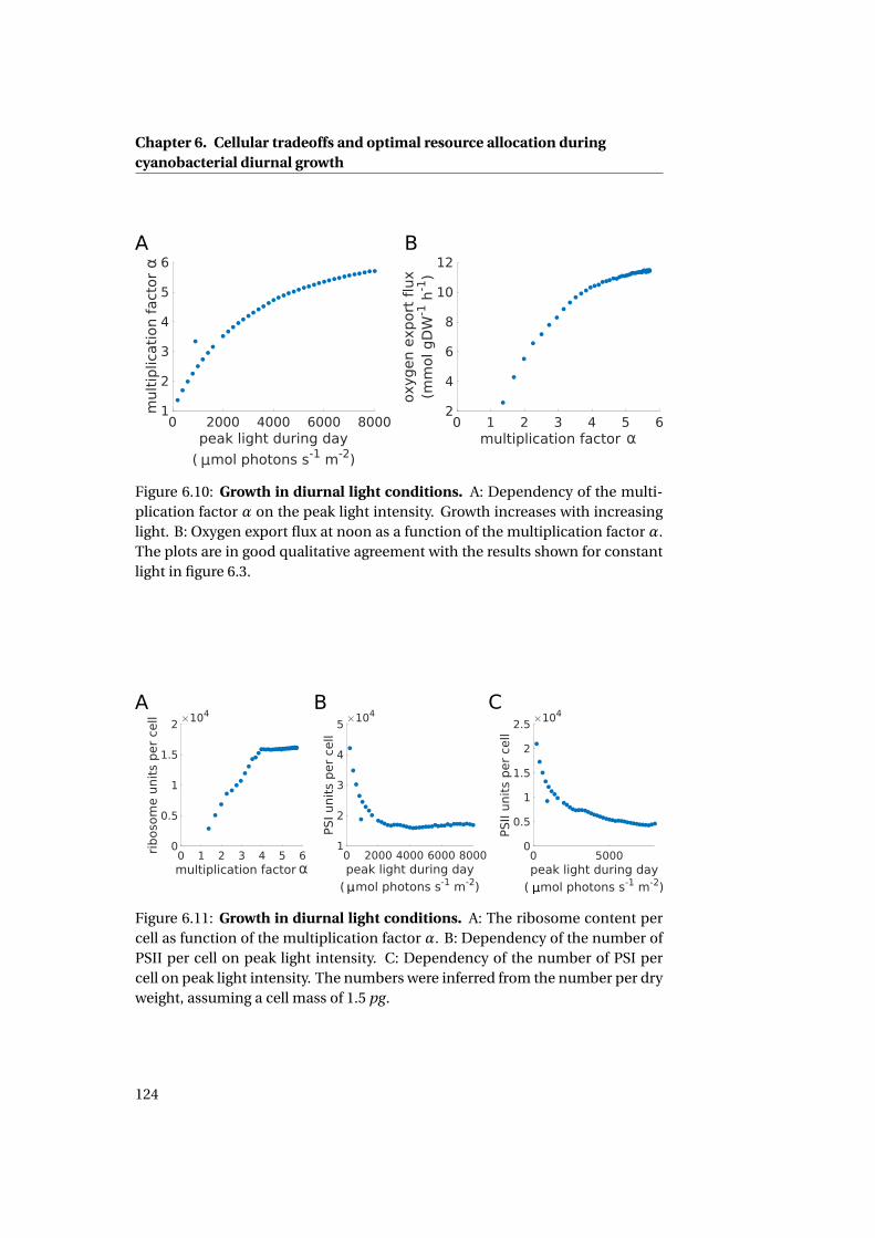
Chapter 6. Cellular tradeoffs and optimal resource allocation duringcyanobacterial diurnal growth
α
αμ
A B
Figure 6.10: Growth in diurnal light conditions. A: Dependency of the multi-plication factor α on the peak light intensity. Growth increases with increasinglight. B: Oxygen export flux at noon as a function of the multiplication factor α.The plots are in good qualitative agreement with the results shown for constantlight in figure 6.3.
αμ μ
A B C
Figure 6.11: Growth in diurnal light conditions. A: The ribosome content percell as function of the multiplication factor α. B: Dependency of the number ofPSII per cell on peak light intensity. C: Dependency of the number of PSI percell on peak light intensity. The numbers were inferred from the number per dryweight, assuming a cell mass of 1.5 pg.
124

Figure 6.12: A solution of the resource allocation problem over a full diurnalcycle. A: Normalized metabolic fluxes as a function of diurnal time. To indi-cate the periodicity of the solution, the beginning of the subsequent light pe-riod is also shown (hours 24-30). We observe a highly coordinated metabolicactivity over a diurnal period. Metabolism is organized into distinct tempo-ral phases, ranging from synthesis of amino acids and pigments, to synthesisof lipids, DNA/RNA and peptidoglycan, to synthesis of co-factors. The func-tional category of each flux is indicated by a black bar in the table adjacentto the plot. B: Excerpt of the light period. The flux values are normalized toRuBisCO flux and scaled to the unit interval. The normalization emphasizesrelative carbon partitioning rather than the dependence of metabolic fluxeson total light input. C: Selected metabolic fluxes and their corresponding ca-pacity bounds. Dashed red lines indicate the enzymatic capacities (propor-tional to enzyme amount). Photosynthesis and reactions of central metabolismclosely follow light availability (e.g. transketolase TKL or PSII). Metabolic ac-tivity during the early light period is dominated by amino acid synthesis (e.g.DA7-P for synthesis of aromatic amino acids, nitrate uptake NITTR, and GTRRtowards chlorophyll). Later, metabolic activity shifts to DNA and RNA syn-thesis (e.g. 5PRPPAT) and lipid synthesis (e.g. 3-OA-ACP-syn.), followed bysynthesis of peptidoglycan (e.g. GF6PAT) and co-factors (e.g. L-Asp-O. to-wards nicotinamide adenine dinucleotide). During night, glycogen is utilizedvia the glycogen phosphorylase (GP). Abbreviations: DAH7-P synthase, 3-deoxy-D-arabino-heptulosonate 7-phosphate synthetase; GP, glycogen phosphory-lase; AO, aspartate oxidase; GF6PAT, glucosamine-fructose-6-phosphate amino-transferase; NITTR, nitrate transporter; THG, transhydrogenase; 5PRPPAT, 5’-phosphoribosylpyrophosphate amidotransferase; GTRR, glutamyl-tRNA reduc-tase; OAAS, 3-oxoacyl-ACP synthase; TKL, transketolase; PSII, photosystem II.

Chapter 6. Cellular tradeoffs and optimal resource allocation duringcyanobacterial diurnal growth
The solution of the resource allocation problem exhibits a highly coordinatedmetabolic activity over a diurnal period: oxygenic photosynthesis is activeduring the light period. Inorganic carbon is imported and assimilated via theCalvin-Benson cycle (anabolism), respiratory components (catabolism) areactive during the dark period. We highlight two results of the model.
First, we observe that growth is dynamic. The instantaneous growth rate, de-fined in equation (4.1), follows a specific pattern over the light period. Thegrowth rate is low in the early morning, increases over the course of the light pe-riod and decreases again towards dusk (figure 6.13). Such a dynamic growth rateover a diurnal cycle was recently reported for the cyanobacterium Synechocystissp. PCC 6803 (Angermayr et al., 2016), and is also observed when the sinusoidallight input is replaced by the square-wave light-dark cycle typically employed inexperiments.
0 6 12 18 24diurnal time (h)
-0.02
0
0.02
0.04
0.06
0.08
0.1
0.12
inst
an
taneous
gro
wth
rate
square-wave light shapesine-wave light shape
Figure 6.13: Instantaneous growth rate (h−1) for reference day using sine-wave and square-wave light input. The instantaneous growth rate is defined
as 1∆t · log
(biomass(ti )
biomass(ti−1)
), where biomass(ti ) is the biomass amount at time point
ti and ∆t = ti − ti−1 (here ∆t = 0.5h). The instantaneous growth rate has re-cently been measured for Syncheocystis sp. PCC 6803 under diurnal conditions(see figure 1A in Angermayr et al. (2016)). Therein, after a lag phase, the growthrate increases until shortly after noon, and decreases again towards the evening.Measurements were done under a square-wave light input. The initial lag phasemight be due to the sudden light increase at dawn, such effects are not capturedby our model. We observe a similar curve under both, sinusoidal, as well assquare-wave light input.
Secondly, we observe that growth is exclusive to the light period. During thenight phase, glycogen is used for cellular maintenance, serving as a substratefor respiration via the oxidative pentose phosphate pathway and ultimately cy-tochrome C oxidase. While this observation is unsurprising given the knowndata on S. elongatus 7942 and other cyanobacteria, we emphasize that cessa-
126

6.4 Results
tion of metabolic activity at dusk is not self-evident but already the result of acellular tradeoff. Limited metabolic activity at night implies not using alreadyexisting capacity in terms of enzymes and ribosomes during dark. The bene-fit of avoiding or reducing the timespan of this idle cellular capacity, however,would require additional storage compounds that must be synthesized prior tothe dark period . This, in turn, would entail additional enzymatic costs in termsof storage synthesis capacity. To demonstrate this tradeoff, we conducted an insilico experiment using a reduced cost for glycogen synthesis and utilization byneglecting the synthesis costs of the respective enzymes. In this case, cellularsynthesis also prevails during the night phase, driven by an increased amountof stored glycogen at dusk (figure 6.14). The experiment, however, also revealsthat the amount of necessary additional storage capacity is significant. The highstorage requirements explain why such behavior is not observed for the originalparameters.
6 12 18 24
A BCO2 uptake
photon uptakeRuBisCO
oxygen exportATPase
FNRcytochrome b6f
cytochrome c oxydaseribosome synth.
DNA synth.lipid synth.
glycogen synth.glycogen use
cell wall synth.pigment synth.cofactor synth.
noncatalytic protein synth.enzyme synth.
PS synth.
Figure 6.14: A hypothetical scenario in which the synthesis and breakdown ofglycogen requires no enzymatic costs. Glycogen synthesis and use are imple-mented using spontaneous reactions. As expected, under these conditions itis energetically more favorable to use synthesis reactions also during the nightphase, thereby lowering capacity requirements during the light phase, at the ex-pense of increased glycogen storage. A: Timing and dynamics of glycogen accu-mulation over the day. The plot shows that synthesis reactions during the nightperiod require a significant amount of glycogen. B: Metabolic activity of key re-actions. Time courses are color-coded and normalized to the unit interval.
6.4.5 Metabolite partitioning during diurnal growth
The results obtained from the resource allocation problem can be compared toknown experimental observations about metabolite partitioning during diurnalgrowth. While no 13C flux measurements over a full diurnal cycle have beenconducted yet, several studies have investigated the transcriptome, proteomeand physiology of S. elongatus PCC 7942 and other cyanobacteria over a full
127

Chapter 6. Cellular tradeoffs and optimal resource allocation duringcyanobacterial diurnal growth
24 h diurnal cycle (Lehmann et al., 2013; Guerreiro et al., 2014; Diamond et al.,2015; Saha et al., 2016). Published transcriptome studies of cyanobacteria typi-cally show global rhythms in gene expression, including a significant reductionof the transcriptional output during the dark period (Ito et al., 2009; Lehmannet al., 2013; Beck et al., 2014). While environmental light-dark cycles are suf-ficient to drive transcriptional and metabolic rhythms, metabolic rhythms arealso influenced by the cyanobacterial circadian clock and persist in cultures un-der constant light (Markson et al., 2013; Pattanayak et al., 2014; Diamond et al.,2015). Several transcriptomic studies described a broad temporal order of di-urnal growth, typically distinguishing between genes peaking at dawn versusgenes peaking at dusk (Ito et al., 2009; Diamond et al., 2015). The former setincludes genes associated with the Calvin-Benson cycle, as well as genes as-sociated with amino acid synthesis. The latter set includes genes associatedwith glycogen mobilization and the oxidative pentose phosphate pathway (Di-amond et al., 2015). The observed temporal order is consistent across differ-ent cyanobacterial strains. For the cyanobacterium Synechocystis sp. PCC 6803,(Saha et al., 2016) report an upregulation of PSI and PSII transcripts, genes foramino acid metabolism, and genes from the Calvin-Benson cycle at the begin-ning of the light period, whereas essential genes for glycogen catabolism showedupregulation in the dark period. (Behrenfeld et al., 2008) report metabolism isdominated by amino acid synthesis between sunrise and noon in a synchro-nized culture of Prochlorococcus PCC 9511.
The results of the resource allocation problem, shown in figure 6.12, closelyreplicate this temporal order. Metabolism at dawn is dominated by amino acidsynthesis and synthesis of pigments. Photosynthetic activity and reactions ofcentral metabolism closely follow light availability. Later in the day, DNA andRNA are synthesized, then lipid, peptidoglycan, and co-factors follow. We notethat synthesis of enzymes can precede reaction flux, for example for the glyco-gen phosphorylase (plot GP in figure 6.12C). Overall, the differences in activitybetween light and dark metabolism, the initiation of amino acid metabolismat dawn, and storage metabolism are in qualitative agreement with reportedmetabolite partitioning during diurnal growth.
However, several caveats limit a direct comparison of individual reaction rates tocurrently available data. Current transcriptomics data are predominantly mea-sured under constant light conditions using synchronized cultures. Such mea-surements aim at discerning the effects of the circadian clock versus light-drivenregulation and conceal actual resource allocation. Furthermore, gene expres-sion is not necessarily indicative of metabolic flux. Measurements also typi-cally involve slow growing cultures, with reduced requirements for de novo pro-tein synthesis. Correspondingly, proteomics measurements typically exhibit re-duced diurnal variability (Waldbauer et al., 2012; Guerreiro et al., 2014) com-pared to transcriptomics data. The qualitative agreement of results obtainedfrom the computational model with transcriptomics data may therefore provide
128

6.4 Results
further incentives for experimental studies to focus on de novo protein synthesisin fast growing cultures – and thereby to enable a quantitative comparison of thetiming of protein synthesis.
6.4.6 The dynamics of glycogen accumulation
Glycogen is the main storage compound in cyanobacteria. Cells accumulateglycogen during the light phase and mobilize it as a source of carbon and energyduring the night. It was recently shown that the timing of glycogen accumula-tion is under tight control of the cyanobacterial circadian clock and disruptionof the clock results in altered glycogen dynamics (Diamond et al., 2015). Wetherefore investigate the dynamics of glycogen accumulation in the context ofthe global resource allocation problem. We note that our simulation does notimpose any ad hoc constraints on the kinetics and timing of glycogen synthesis.Rather, accumulation of glycogen is a consequence of optimal resource alloca-tion. Figure 6.15 shows the time course of glycogen accumulation obtained fromthe global resource allocation problem over a diurnal period, as well as the pre-dicted carbon partitioning ratio during the light period.
μ
Figure 6.15: Timing and dynamics of glycogen accumulation over a full diurnalcycle. After a brief lag phase, cells accumulate glycogen during the light periodand mobilize it as a source of carbon and energy during the night. Shown areabsolute amounts of stored glycogen per gram dry weight, as well as the car-bon partitioning ratio. We define the carbon partitioning ratio as the ratio be-tween the glycogen synthesis flux and the carbon assimilation flux (RuBisCO),weighted by the corresponding stoichiometries.
The constant rate of glycogen accumulation through the light period is in excel-lent agreement with recent data on S. elongatus PCC 7942 (Diamond et al., 2015)and Synechocystis sp. PCC 6803 (Saha et al., 2016). To verify the robustness ofour approach, and since most experimental studies use a square-wave light in-
129

Chapter 6. Cellular tradeoffs and optimal resource allocation duringcyanobacterial diurnal growth
tensity, rather than a sinusoidal function, we also investigate glycogen accumu-lation using a square-wave light function, resulting in a similar functional form(figure 6.16).
μ
Figure 6.16: Glycogen under a square light wave. The overall shape of the curveremains robust. We note that results for a square-wave input have to be inter-preted with caution. Our approach is based on the assumption that S. elonga-tus evolved an appropriate regulatory scheme that coordinates its metabolismin their natural diurnal environments. For experiments in an environment dif-ferent from the natural environment, the evolved regulatory scheme is still inplace. We therefore expect to observe a superposition of the effects of the newenvironment and the original (evolved) regulatory scheme.
We emphasize that the linear slope is not self-evident, but emerges as a trade-off between at least two conflicting objectives: (i) minimal withdrawal of carbonduring the early growth period, when the resources could be invested in creat-ing enzymatic and translational capacity that can be used throughout the dayversus (ii) investing a minimal amount of carbon resources into the enzymesneeded for glycogen synthesis. While the former objective favors withdrawal ofcarbon for glycogen synthesis later in the day, the later justifies a constant car-bon withdrawal for storage synthesis throughout the light period. To the best ofour knowledge, the initial lag phase has not yet been noted experimentally, butmight provide a stimulus for further experimental evaluation.
6.4.7 Glycogen accumulation for variable day lengths
To highlight glycogen accumulation as a systemic property, we also investigatethe minimal amount of accumulated glycogen for different photoperiods. Fig-ure 6.17A shows the resulting time courses for different lengths of day versusnight periods. Figure 6.17B shows the minimal amount of glycogen required at
130

6.5 Discussion
the end of the light period.
0 6 12 18 24diurnal time (h)
0
0.02
0.04
0.06
0.08gly
cogen a
mou
nt
(g)
6 h8 h10 h12 h14 h
6 9 12 15day length (h)
0
0.02
0.04
0.06
0.08
0.1
min
imal gly
cogen a
t dusk
(g)
A B
Figure 6.17: Glycogen for different day lengths. A: Time courses of glycogenaccumulation for different lengths of the light period (day length). B: Mini-mal glycogen requirements for different day lengths. Peak glycogen content isalways observed at dusk. While the minimal amount of glycogen required atdusk exhibits a clear bound, cells can accumulate more glycogen with no dis-cernible effects on overall growth yield. Higher glycogen at dusk implies in-creased metabolic activity shortly before dawn at the expense of slightly reducedsynthesis reactions during the light period.
The overall form of glycogen accumulation remains largely identical. We note,however, that the amount of glycogen required at dusk exhibits a certain plas-ticity. Firstly, if the night period is doubled, slightly less than twice the glycogenis required to sustain night metabolism. Secondly, while the minimal amountof glycogen required at dusk exhibits a clear bound, cells can accumulate moreglycogen with no discernible effects on overall growth. In this case, certain syn-thesis tasks, in particular lipid synthesis, can be postponed to the end of thenight period, thereby requiring less enzyme capacity during the day at the ex-pense of an increased glycogen storage at dusk.
6.5 DiscussionPhototrophic growth under diurnal conditions requires a precise coordinationof metabolic processes – and the resulting constraints and tradeoffs are chal-lenging to describe using constraint-based analysis and conventional FBA (Hen-son, 2015). We have developed a genome-scale resource allocation model thatallowed us to investigate the stoichiometric and energetic constraints of diurnalphototrophic growth in the context of a global resource allocation problem. Wefocused on the net stoichiometric and energetic implications of diurnal growthon the de novo synthesis of proteins and other cellular macromolecules.
Our aim was a prediction of optimal diurnal resource allocation: how are
131

Chapter 6. Cellular tradeoffs and optimal resource allocation duringcyanobacterial diurnal growth
metabolism and the synthesis reactions of cellular macromolecules organizedover a full diurnal cycle? What is the optimal timing of glycogen accumulationduring the light phase? From the perspective of cellular resource allocation,these questions can be asked without detailed knowledge about regulatorymechanisms and their corresponding kinetic parameters.
The results obtained from the computational model allowed us to pinpointseveral energetic tradeoffs and constraints related to diurnal growth. Overall,the model-derived time courses are in good qualitative agreement with pre-vious experimental observations about flux partitioning in S. elongatus PCC7942 and other cyanobacteria. Growth is dynamic and takes place during thelight phase. Carbon fixation and the reactions of central metabolism largelyfollow light availability. The synthesis of amino acids and pigments dominatemetabolism during the early light period, whereas other synthesis reactionspeak at later time points. In the absence of light, almost all metabolic activityceases, and cellular metabolism is dominated by respiratory activity. Whilewell-known experimentally, we emphasize that in the computational model thecessation of metabolic activity during darkness is a consequence of a tradeoffbetween the cost of unused enzymatic capacity during darkness versus thecost of additional storage that would be required for synthesis reactions totake place in the absence of light. In this respect, the function of the storagecompound glycogen is analogous to a cellular battery or capacitor: we expectthat if glycogen synthesis and utilization would not entail additional enzymatic(and other) costs, synthesis reactions would continue during the night. Withinour computational framework we confirmed this hypothesis using an in silicoexperiment with modified enzyme synthesis costs.
For our reference parameters, the predicted timing characteristics of glycogenaccumulation matched recent experimental observations (Diamond et al., 2015;Saha et al., 2016). The emergent dynamics of glycogen accumulation point tothe role of the circadian oscillator to modulate metabolite partitioning duringgrowth. It has been shown recently that the circadian oscillator controls the tim-ing of glycogen accumulation such that it occurs at a constant rate through thelight period. A disrupted clock results in increased glycogen accumulation earlyin the day (Diamond et al., 2015). The disrupted pattern of glycogen accumula-tion is indeed significantly different from the optimal profile predicted here. Amanifest hypothesis is therefore that cyanobacterial growth is organized accord-ing to a temporal program that evolved to maximize growth in a periodic envi-ronment, and that the circadian clock is a regulatory circuit that modulates thetranscriptional program of the cell to approach this metabolic optimum. Mis-alignments between metabolism, clock and environmental cycles will thereforeresult in impaired growth, as observed by (Lambert et al., 2016).
Recent analyses (Goelzer et al., 2015; Price et al., 2016; Yang et al., 2016) revealseveral interesting differences with respect to our results. The model-derivedgrowth rates for E. coli corresponding to an optimally allocated proteome were
132
6.5 Discussion
consistently higher than the experimentally measured rates. In the model, thelatter could be supported with 95% less proteome under certain conditions(Yang et al., 2016). This was attributed to cellular “bet hedging” in (generalist)wild-type E. coli against unknown environmental challenges. Furthermore,significant protein production without detectable growth benefit was observedexperimentally (Yang et al., 2016; Price et al., 2016).
In contrast, the model-derived maximal growth rates we report here are withinthe range of the (maximal) growth rates observed for S. elongatus PCC 7942, eventhough actual growth rates observed in a laboratory are typically significantlyslower (Kuan et al., 2015).
We note that the resource allocation problem only provides upper bounds forthe growth rate, assuming an optimally-allocated metabolism, and does not in-corporate several detrimental factors, such as light damage and possible pho-toinhibition. Thus, the close correspondence between observed and model-derived values suggests that cyanobacterial metabolism operates close to op-timality – at least in experiments designed for rapid growth.
The model-derived maximal growth rates should be interpreted as an order-of-magnitude approximation, not as a precise estimate. For example, a major un-known factor is the relative amount of non-catalytic proteins, estimated to be upto 55% of total protein for slow growing cells (Guerreiro et al., 2014). We hypoth-esize that for fast growing cells this percentage is considerably lower. The impactof non-catalytic proteins as (condition-specific) niche-adaptive proteins on themaximal growth rate was already discussed in (Burnap, 2015). The question towhat extent slow growing cyanobacteria perform cellular bet hedging similar toE. coli and how the allocation of proteome to non-growth-related processes cor-relates with resistance to adverse environmental and sudden stress conditionsremains a question for further research – with implications for biotechnologicalstrain design.
133


Chapter 7
Optimal resource allocation inyeast under dynamicallychanging environments
The work presented in this chapter has been done within the Europeanproject ROBUSTYEAST, a collaboration of
• Freie Universität Berlin (Alexander Bockmayr)• Vrije Universiteit Amsterdam (Frank Bruggeman)• École polytechnique fédérale de Lausanne (Vassily Hatzimanikatis)• Katholieke Universiteit Leuven (Steffen Waldherr)
This project aims at revealing the principles for robustness of metabolism toextracellular nutrient dynamics in yeast using systems biology approaches.Experimental data used in this chapter was provided by Johan van Heerden.
Microbial strains used in biotechnological production pipelines at industry-scale need to fulfill two key requirements: they need to be able to producethe products of interest at high yield, and they need to be robust to the localheterogeneities arising in large industrial bioreactors, especially to transientlimitations in nutrient sources and oxygen.
For the former requirement of high yield several systems biology approacheshave been developed to obtain very productive strains (Hädicke and Klamt,2011; Kim et al., 2011; Jungreuthmayer and Zanghellini, 2012; Trinh, 2012;Gruchattka et al., 2013; Erdrich et al., 2014; von Kamp and Klamt, 2014; Klamtand Mahadevan, 2015). However, such strain optimization strategies reportstrains that are optimized for steady-state conditions, and not for the dynamicalconditions present in industry-scale bioreactors. As a result, these strains are
135

Chapter 7. Optimal resource allocation in yeast under dynamically changingenvironments
very rarely capable of overcoming the nutrient and oxygen shifts arising fromimperfect mixing. Indeed it has recently been shown that individual cellsrespond very differently to changes in nutrient availability. This gives rise toa subpopulation adapting to the new conditions and resuming growth, whileanother subpopulation dies out, and thus induces a huge productivity loss (vanHeerden et al., 2014).
We, in the ROBUSTYEAST consortium, believe that one element that makes adifference in survival is the choice of the organism between being a generalistand being a specialist. That means a choice between investing resources intoproteins that are unnecessary at the moment but may become useful later ver-sus only producing the proteins needed at the moment. Besides that, we wantto understand how does the organism adapt to the new environment.
For this purpose, we built a dynamic resource allocation model of the yeastSaccharomyces cerevisiae. As a start, we validated the growth rates obtainedfrom our model using experimental data provided by Johan van Heerden, asexplained in section 7.3.1. We have obtained a very good agreement betweenmodel and data, without any parameter changes.
We continued by studying how wildtype yeast adapts to changes in the environ-ment.
Next, we have designed a series of studies of in silico yeast knock-out mutantstrains in dynamic environments. The idea behind this is that, mutants who areviable in constant conditions, but do not survive environment shifts are miss-ing a gene that is vital for surviving the transition. Thus, we provide a list ofcandidate genes critical for survival in dynamic conditions. This list remains tobe validated once data from the experimental partners in the ROBUSTYEASTproject is available.
7.1 Model building
7.1.1 Choice of reconstruction and model reduction
The first step in building a resource allocation model for yeast was choosing ametabolic reconstruction to start with. Since 2003, more than 25 genome-scalemetabolic network reconstructions of yeast have been published (Förster et al.,2003b; Duarte et al., 2004; Krieger et al., 2004; Kuepfer et al., 2005; Herrgård et al.,2006; Hjersted and Henson, 2006; Herrgård et al., 2008; Nookaew et al., 2008; Moet al., 2009; Aho et al., 2010; Dobson et al., 2010; Zomorrodi and Maranas, 2010;Costenoble et al., 2011; Matsuda et al., 2011; Swainston et al., 2011; Szappanoset al., 2011; Celton et al., 2012; Heavner et al., 2012; Aung et al., 2013; Heavneret al., 2013; Österlund et al., 2013), some of which were reviewed in (Heavner andPrice, 2015). The genome-scale models range in size between iND750 (Duarteet al., 2004) with 1061 metabolites and 1266 reactions and Yeast 7 (Aung et al.,2013) with 2220 metabolites and 3498 reactions.
136

7.1 Model building
Based on this wide variety, one would most likely choose the newest consen-sus model, Yeast 7, as this contains the most recent and comprehensive anno-tations. However, the size of this model is too large to allow a dynamic resourceallocation analysis using deFBA. One can reduce this model, while preservingdesired functionalities, as described in chapter 4 using a network reducer. How-ever, after running the minimal network finder tool for more than 24 hours, westill could not obtain a reduction. Therefore, we have decided to use Yeast 6(Heavner et al., 2013), which we were able to reduce using the minimal networkfinder from (Röhl and Bockmayr, 2017).
We focus, just as the experimental partners in ROBUSTYEAST, on growth in min-imal Verduyn medium, whose composition we detail in table A6 in Appendix D.Additionally, we would like to study yeast both in aerobic and anaerobic condi-tions. According to (Ishtar Snoek and Yde Steensma, 2007), yeast needs sterolsand unsaturated fatty acids in the medium to grow anaerobically. Therefore,additional medium components were added. For a complete list of these com-ponents see table A7 in Appendix D.
The network reducer in (Röhl and Bockmayr, 2017) uses a mixed integer linearprogramming approach to compute the minimal subnetwork of a given networkthat still preserves some user-given functionalities. For instance, one function-ality could be that the reduced network retains 99% of the original network’sflux through the biomass reaction in a fixed environment. Another functional-ity could be that certain metabolites or reactions should be kept in the reducednetwork.
Therefore, to reduce the Yeast 6 model, we have defined a list a functionalitieswhich should be kept in the reduced model:
• The reduced model should display at least 99% of the Yeast 6 biomass fluxin the following environmental conditions:
– aerobic glucose
– anaerobic glucose
– aerobic galactose
– anaerobic galactose
• The reduced model should retain the fermentation pathway.
We obtained a reduced network with 454 metabolites, 438 reactions, and 429genes, which can be found at https://ndownloader.figshare.com/files/8653207. As already seen in chapter 6, it is possible to study networks of thissize using dynamic resource allocation tools.
After the reduction, we wanted to include as much as possible from the newinformation in Yeast 7 in our reduced network. Moreover, we made sure that
137

Chapter 7. Optimal resource allocation in yeast under dynamically changingenvironments
the network can consume possible by-products of overflow metabolism such asethanol or glycerol, as is the case in reality. Therefore, the following additionalchanges to the network have been made. Note that the reactions in Yeast 6 are asubset of those in Yeast 7, and the reaction IDs are the same.
• reaction r_1117 has been constrained to be irreversible (Pereira et al.,2016)
• reactions r_2111 and r_2133 (biomass) have been removed
• putrescine cycling through reactions r_1250 and r_1251 has been removed
• reaction r_0364 has been constrained to be irreversible as it has a stronglynegative Gibbs free energy at physiological pH and reactant concentra-tions: ∆r G ′m = −55.4kJ/mol computed using the eQuilibrator resource(Flamholz et al., 2012)
• reactions r_1130 and r_1131 have been constrained to be irreversible(Marobbio et al., 2006)
• reactions r_0735 and r_0736 have been constrained to be irreversible(Miziorko, 2011)
• reaction r_0143 has been constrained to be irreversible as it has a stronglynegative Gibbs free energy at physiological pH and reactant concentra-tions: ∆r G ′m = −48.7kJ/mol computed using the eQuilibrator resource(Flamholz et al., 2012)
• reaction r_1245 has been constrained to be irreversible (Hamel et al., 2004)
• reaction r_0962 has been constrained to be irreversible (Portela et al.,2006)
• H+ was removed from reaction r_0507 for charge balancing (Aung et al.,2013)
• GDH2 (r_0470) has been set to irreversible in the backwards direction(Aung et al., 2013)
• mitochondrial ADP/ATP transporter (r_1110) does not cotransport pro-tons (Klingenberg, 1980; Vozza et al., 2004)
• ATP synthase (r_0226) moves 4 cytoplasmic protons (Aung et al., 2013)
• NADH:ubiquinone oxidoreductase (r_0773) is not proton translocating(Velázquez and Pardo, 2001)
• malic enzyme (r_0718) is not NAD+-, but NADP+-dependent (Boles et al.,1998; dos Santos et al., 2004)
• changed proton stoichiometry for cytochrome oxidase (r_0438) (Post-mus et al., 2011) and for ubiquinol cytochrome-c reductase (r_0439)(Trumpower, 1990)
• L-aminoadipate-semialdehyde dehydrogenase (r_0678) requires ATP(Zabriskie and Jackson, 2000)
• metabolites exchanged through the mitochondrial transporter r_1099were changed to 2-oxoadipate and 2-oxoglutarate and the reaction wasset as reversible (Palmieri et al., 2001)
138

7.1 Model building
• alcohol dehydrogenase (r_0163, ethanol to acetaldehyde), acetaldehydetransport (r_1632), aldehyde dehydrogenase (r_0174, r_0175), acetyl-CoAsynthetase (r_0113), adenylate kinase (r_0149), and cytosolic glycerol 3-phosphate dehydrogenase (r_0491), which had not been retained by thereduction, were added back to ensure the model can consume overflowmetabolism by-products
• fructose bisphosphatase (r_0449) and phosphoenolpyruvate carboxyki-nase (r_0884), which had not been retained by the reduction, were addedback to ensure the model can run gluconeogenesis
• glucan 1,4-α-glucosidase (r_0463), glycogen phosphorylase (r_0511), andα,α-trehalase (r_0194), which had not been retained by the reduction,were added back to ensure the model can consume the storage productsglycogen and trehalose
7.1.2 The macromolecules of autocatalytic growth
Starting from the reduced network, a deFBA model of yeast has been con-structed, following the guidelines in chapter 4.
Ribosomes
The ribosome turnover rate was set to 10 attached amino acids per second ac-cording to data in (Karpinets et al., 2006; Milo and Phillips, 2015), while the listof ribosomal proteins was sourced from the Ribosomal Protein Gene Database(Nakao et al., 2004) and is displayed in table A8 in Appendix D.
Enzyme subunit stoichiometry
The subunit stoichiometry of all enzymes has been sourced manually fromUniProtKB (UniProt Consortium, 2014) and from the Saccharomyces GenomeDatabase (Cherry et al., 2012). The SBML file, generated in the format describedin section 4.8, is in the process of being uploaded to FairdomHub.
Storage
The two main storage molecules of yeast are glycogen and trehalose, which wedenote by G and TH . Just as in the Synechococcus model in the previous chapter,these are allowed to accumulate and may be consumed if available.
Noncatalytic biomass
The noncatalytic (quota) biomass has been organized into six quota metabo-lites: noncatalytic proteins, RNA, DNA, cell wall, lipids and small molecules.The production reactions for these quota metabolites are shown in table A9 inAppendix D.
139

Chapter 7. Optimal resource allocation in yeast under dynamically changingenvironments
7.2 Model constraints and objective
7.2.1 Constraints
Steady-state versus time-dependent quantities
As before, we assume internal metabolites are at a quasi-steady-state with re-spect to the macromolecules and environment dynamics. As in chapter 6, wehave
dnM (t )
d t= SM∗v(t ) = 0, (7.1)
anddni (t )
d t= Si∗v(t ), ∀i ∈ E ∪Q∪G ∪TH . (7.2)
Enzyme amounts constrain reaction rates
Enzyme amounts constrain reaction rates within the metabolic network as ex-plained in chapter 2. Turnover numbers for metabolic enzymes were retrievedfrom the BRENDA database (Schomburg et al., 2013) and manually sourcedfrom the literature. The turnover numbers for glucose and galactose uptakewere set to 200 s−1 according to data in (Ye et al., 2001).
For irreversible enzyme-catalyzed reactions j , our constraint then reads
v j (t ) ≤ k jcat nE j (t ), (7.3)
at all time points t . In the case of reversible reactions, both directions are con-strained
v j (t ) ≤ k j+cat nE j (t ), v j (t ) ≥−k j−
cat nE j (t ), (7.4)
where k j+cat and k j−
cat are the turnover rates for the forward and reverse directionrespectively. We impose these two constraints at each time point t for each re-versible reaction j . The constraints apply only for enzyme-catalyzed reactions.Rates of spontaneous reactions remain free of these bounds.
In case several reactions are catalyzed by the same enzyme, their total fluxweighted by the inverse of the respective turnover numbers is bound by theenzyme amount. Such a situation happens, for instance, in the case of theribosome, as detailed in the previous chapters. Enzyme synthesis reactionsare irreversible and hence the bound is only applied for the forward directionsof the reactions, while the reverse directions are prohibited using a lower fluxbound of zero at all time points.
Extracellular metabolites
We distinguish between nonlimiting extracellular metabolites (present in satu-ration amounts) and part of the Verduyn medium
140

7.2 Model constraints and objective
• O2
• H+
• H2O• CO2
• ammonium• phosphate• sulphate• (R)-pantothenate• 14-demethyllanosterol• ergosta-5,7,22,24(28)-tetraen-3beta-ol• fecosterol• myo-inositol• lanosterol• zymosterol
and nutrient sources the may deplete
• glucose• galactose• ethanol
The amounts of the latter are modeled dynamically following the uptake by themetabolic network as
dnX (t )
d t= SX∗v(t ), (7.5)
where X denotes the set of extracellular metabolites available in limitedamounts. The uptake of extracellular metabolites present at saturation is onlyconstrained by the existing transporter capacity and its catalytic efficiency.
Amounts of quota compounds
The initial values for the six quota compounds are set to be equal to their corre-sponding amounts in 1 gram dry weight of yeast cells and displayed in table A10in Appendix D. We denote their initial amounts as the vector q0, and require thatthese proportions are kept as lower bounds for quota amounts throughout thesimulation time as
nQ(t ) ≥ q0∑
i∈E∪Q∪G∪THMWi ni (t ). (7.6)
According to the data in (De Godoy et al., 2008), the catalytic proteins whichare modeled explicitly in our model sum up to a fraction of 0.40561 of the totalproteome of yeast grown in minimal medium. In the biomass reaction of Yeast6 we find that proteins make up 0.466298 grams in one gram dry weight of cells.Thus, we have set the noncatalytic protein quota requirement to (1−0.40561) ·0.466298 = 0.27716 g/gDW .
141
Chapter 7. Optimal resource allocation in yeast under dynamically changingenvironments
As before, together with metabolic proteins, glycogen, and trehalose, the initialcomposition vector adds up to one gram, and thus we obtain the additional con-straint ∑
i∈Q
ni (t0)+ ∑i∈E
ni (t0) ·MWi +nG (t0)+nTH (t0) = 1. (7.7)
Maintenance
No ATP maintenance has been enforced since the growth rates obtained in themodel are close to those observed in experiments, as we will show in the resultssection.
Time discretization
As detailed in chapter 5, we discretize time using the implicit midpoint rule.Derivatives n and fluxes v are evaluated at the middle of the discretization in-tervals, while macromolecule amounts n are evaluated at the ends of the dis-cretization intervals.
Environment shifts
To analyze how yeast deals with environment shifts, we distinguish between twotypes of shifts:
• Shifts in extracellular metabolites present at saturation. In case wemodel that an extracellular metabolite that is not a nutrient is no longerpresent in the environment for a time period, we simply block therespective transporter by imposing its lower and upper flux bounds to bezero.
• Shifts in nutrient sources. In case we model shifts in nutrient sources,such as a shift from glucose to galactose medium, we impose at the shifttime point tshift the desired bounds on the respective extracellular nutri-ent amounts. In addition, for the nutrient removed from the medium, weneed to remove the constraint that links its amount at tshift with its amountat the time point right before tshift , as this constraint is no longer satisfied.
7.2.2 Objective
Since yeast does not follow a light availability periodicity as was the case forcyanobacteria, we do not use cFBA, but deFBA to study dynamic resource allo-cation in this model. Thus, as detailed in chapters 2 and 5, we use the objective
maxn(t ),n(t ),v(t )
∫ t f
0
∑i∈E
MWi ni (t )d t . (7.8)
142

7.3 Results
To avoid the side effects of including storage and noncatalytic compounds in theobjective, analyzed in (Waldherr and Lindhorst, 2017), we only include enzymesin the objective. Note that, since quota amounts are required to have a certainfraction of total biomass at each time point, they are implicitly maximized usingthis objective.
7.2.3 deFBA vs. short term deFBA
Since through a global optimization approach such as deFBA the system alreadyknows at the start of the simulation time whether and when an environmentshift will occur, an important method for these studies was short term deFBA,which we briefly explained in chapter 2. This way, by only using a limited predic-tion horizon, the system only detects a nutrient shift shortly before the shift ac-tually happens, thereby mimicking the behavior of real cells (Kochanowski et al.,2013).
7.2.4 Sudden shifts
Sudden environment shifts, for example from environment A to environmentB, are implemented using two chained deFBA problems, one for each environ-ment. The initial biomass amounts for the second deFBA problem, i.e., in envi-ronment B, are set to be equal to the last computed biomass amounts in envi-ronment A, i.e., to nE∪G∪TH (t A
f ) where t Af is the total simulation time in environ-
ment A.
Since the condition number of a typical deFBA problem for yeast was lower, in-dicating a better conditioning of the LP problem, all simulations were performedusing the CPLEX Optimization Studio version 12.2.
7.3 Results
Prior to studying yeast under dynamic environments, we validate our modelagainst growth rate experimental data obtained in the same (constant) environ-ment.
7.3.1 Growth in constant environmental conditions
Figures 7.1-7.3 provide a comparison between the experimental and model-derived growth rates in aerobic glucose, aerobic galactose, and anaerobicglucose minimal Verduyn medium. We observe that the model provides arelatively tight upper bound on the experimental growth rates. This is what weexpect, as the model provides an optimal solution that may not be reached inthe lab. We have therefore decided to not add any additional ATP maintenancerequirement to the model.
143

Chapter 7. Optimal resource allocation in yeast under dynamically changingenvironments
A Blo
g o
pti
cal d
ensi
ty (
unit
less
)
time (h) time (h)lo
g t
ota
l b
iom
ass
(g
)Figure 7.1: Comparison between the experimental and model-derived growthrates in aerobic glucose Verduyn medium. A. Log optical density of four batchcultures of yeast grown in aerobic minimal Verduyn medium enriched withsterols and glucose. The derived growth rates were obtained by fitting a linethrough the data points. B. Log of model-derived total biomass for the samemedium computed using deFBA. The model-derived growth rate was obtainedby computing the instantaneous growth rate.
A B
log o
pti
cal densi
ty (
unit
less
)
log t
ota
l bio
mass
(g)
time (h) time (h)
Figure 7.2: Comparison between the experimental and model-derived growthrates in aerobic galactose Verduyn medium. A. Log optical density of fourbatch cultures of yeast grown in aerobic minimal Verduyn medium enrichedwith sterols and galactose. The derived growth rates were obtained by fitting aline through the data points. B. Log of model-derived total biomass for the samemedium computed using deFBA. The model-derived growth rate was obtainedby computing the instantaneous growth rate.
7.3.2 Overflow metabolism is an optimal behavior from a resource al-location perspective
To display even more the very good qualitative agreement between model anddata, we show in figure 7.4 the extracellular glucose and ethanol concentrations144

7.3 Results
A B
log o
pti
cal densi
ty (
unit
less
)
log t
ota
l bio
mass
(g)
time (h) time (h)
Figure 7.3: Comparison between the experimental and model-derived growthrates in anaerobic glucose Verduyn medium. A. Log optical density of fourbatch cultures of yeast grown in anaerobic minimal Verduyn medium enrichedwith sterols and glucose. The derived growth rates were obtained by fitting aline through the data points. B. Log of model-derived total biomass for the samemedium computed using deFBA. The model-derived growth rate was obtainedby computing the instantaneous growth rate.
in aerobic glucose conditions, measured using high performance liquid chro-matography, as well as their model-derived extracellular amount counterparts.We note that a quantitative comparison of extracellular metabolite amountsis not possible here due to unit mismatch between data (concentrations) andmodel-derived quantities (molar amounts).
In addition to the good qualitative agreement, figure 7.4 also shows that themodel ferments glucose even in the presence of oxygen, phenomenon alsoknown in the literature as “overflow metabolism”. This indicates that, althoughoften termed “wasteful”, fermentation in aerobic conditions is the best strategyfor optimizing growth from a resource allocation perspective, consistent withthe conclusions in (Molenaar et al., 2009).
To understand the growth advantage offered by fermentation over respiration,we have simulated the model under the same conditions as before, but withthe ethanol export reaction blocked. This way, we have essentially blocked thewhole fermentation pathway, as ethanol cannot be accumulated inside the celldue to the quasi-steady-state constraint on internal metabolites. The resultinginstantaneous growth rate stabilized at a value of 0.37 s−1, which is 10% lowerthan the growth rate obtained when fermentation was allowed (0.41 s−1).
However, the ideal strategy in aerobic glucose conditions seems to not be exclu-sively fermentation. Instead, a small flux through the respiratory pathway canalso be observed. This brings a small growth advantage and is also the reasonwhy the model derived growth rate in anaerobic glucose conditions is slightly
145

Chapter 7. Optimal resource allocation in yeast under dynamically changingenvironments
18 20 22 24 26time (h)
0
20
40
60
80
100
extr
ace
llula
r co
nce
ntr
ati
on (
mM
)
reactor 1, glucosereactor 2, glucosereactor 3, glucosereactor 4, glucosereactor 1, ethanolreactor 2, ethanolreactor 3, ethanolreactor 4, ethanol
0 10 20 30time (h)
0
500
1000
1500
2000
extr
ace
llula
r am
ount
(mm
ol)
model, glucosemodel, ethanol
A B
Figure 7.4: Comparison between the experimental and model-derived extra-cellular glucose and ethanol amounts in aerobic glucose Verduyn medium. A.Extracellular glucose and ethanol concentrations measured in the laboratory byhigh performance liquid chromatography, corresponding to the reactors in fig-ure 7.1. B. Model-derived extracellular glucose and ethanol amounts computedusing deFBA.
lower than the growth rate obtained when oxygen is present (figures 7.1 and 7.3).
7.3.3 Diauxie is an optimal behavior from a resource allocation per-spective
Another well-known phenomenon in yeast is the diauxie. This manifests whenyeast grows in a batch culture with a mixture of two sugars as nutrient source(typically glucose-galactose). Instead of metabolizing both sugars simultane-ously, some yeasts, including Saccharomyces cerevisiae, consume glucose first,and then galactose, resulting in two separate growth phases (New et al., 2014;Siegal, 2015).
The diauxie is often considered to be a consequence of selection to minimize ex-pression of “useless” metabolic pathways when a nutrient that can be more ef-ficiently used is present in the medium (Magasanik, 1961; MacLean, 2007). Thismeans that also from a resource allocation perspective it must be more efficientto metabolize the sugars sequentially rather than at the same time. We havetested this hypothesis using our resource allocation model. Indeed, although themodel does not account for any regulatory mechanisms, and although deFBAhas global knowledge and can thus “foresee” that glucose will run out, the sug-ars are still consumed sequentially, as shown in figure 7.5.
146
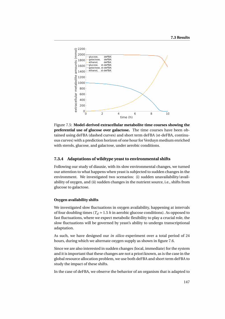
7.3 Results
0 2 4 6 8 10time (h)
0
200
400
600
800
1000
1200
1400
1600
1800
2000
2200
extr
ace
llula
r m
eta
bolit
e a
mounts
(m
mol)
glucose, deFBAgalactose, deFBAethanol, deFBAglucose, st-deFBAgalactose, st-deFBAethanol, st-deFBA
Figure 7.5: Model-derived extracellular metabolite time courses showing thepreferential use of glucose over galactose. The time courses have been ob-tained using deFBA (dashed curves) and short term deFBA (st-deFBA, continu-ous curves) with a prediction horizon of one hour for Verduyn medium enrichedwith sterols, glucose, and galactose, under aerobic conditions.
7.3.4 Adaptations of wildtype yeast to environmental shifts
Following our study of diauxie, with its slow environmental changes, we turnedour attention to what happens when yeast is subjected to sudden changes in theenvironment. We investigated two scenarios: (i) sudden unavailability/avail-ability of oxygen, and (ii) sudden changes in the nutrient source, i.e., shifts fromglucose to galactose.
Oxygen availability shifts
We investigated slow fluctuations in oxygen availability, happening at intervalsof four doubling times (Td ' 1.5 h in aerobic glucose conditions). As opposed tofast fluctuations, where we expect metabolic flexibility to play a crucial role, theslow fluctuations will be governed by yeast’s ability to undergo transcriptionaladaptation.
As such, we have designed our in silico experiment over a total period of 24hours, during which we alternate oxygen supply as shown in figure 7.6.
Since we are also interested in sudden changes (local, immediate) for the systemand it is important that these changes are not a priori known, as is the case in theglobal resource allocation problem, we use both deFBA and short term deFBA tostudy the impact of these shifts.
In the case of deFBA, we observe the behavior of an organism that is adapted to
147

Chapter 7. Optimal resource allocation in yeast under dynamically changingenvironments
off
on
6 12 18 24
time (h)ox
ygen
supp
lyFigure 7.6: Timing of shifts in oxygen availability. The shifts are implementedin the model using temporary zero bounds on the oxygen uptake flux during theperiod when the oxygen supply is off.
a dynamic environment, so it expects the shifts to arise and has prior knowledgeof them.
Short term deFBA shows us how an organism that senses these shifts for the firsttime shortly before they happen (a maximum of one hour prediction horizon)behaves.
A third case is when the organism is a specialist, adapted to growth in constantenvironment, and is then confronted for the first time with a sudden environ-mental shift, without any prior knowledge. For implementing the third case asequence of deFBA problems was solved, one for each environment window(i.e., the windows 0−6, 6−12, 12−18, and 18−24 hours). For each environmentwindow we solve a deFBA problem, imposing as initial condition the biomasscomposition at the end of the previous window. For the first window, the initialbiomass composition is free, but has to obey the constraints on quota and totalmass mentioned in section 7.2.1.
Our first observation is that in all cases growth is dynamic (figure 7.7). In suddenshifts, as well as with a short prediction horizon (1 hour resp. 30 minutes), weobserve adaptation periods before the maximal growth rate is achieved in eachshift window.
The results in figure 7.7 highlight two facts. First, even if the system has globalknowledge about when shifts will occur, there is still a small adaptation pe-riod before the maximal growth rate in the new environment is attained (deFBAcurve). In case of small prediction horizons ahead of the shift, enzymes neededin the new environment are synthesized gradually after the shift at the expenseof a lower growth rate. The simulation with sudden environment shifts displaysthe longest adaptation period in the new environment.
Second, an increase in the prediction horizon (and hence in the preparationtime for the new environment) results in a slight increase in growth rate, butis not sufficient for yeast to be fully prepared for the new conditions.
Another important observation is that the system maintains a linear relation-ship between the growth rate and the amount of ribosome units throughout the
148

7.3 Results
0 6 12 18 24time (h)
0.3
0.32
0.34
0.36
0.38
0.4
0.42
0.44
0.46
inst
an
taneous
gro
wth
rate
(h
-1)
sudden shiftprediction horizon 0.5hprediction horizon 1hprediction horizon 24h (deFBA)
Figure 7.7: Dynamics of the growth rate following the shifts in oxygen avail-ability from figure 7.6. Shown are the growth rate profiles obtained from a sud-den shift (two sequential deFBA problems with a sudden environment change,continuous curve), using short term deFBA with prediction horizon of half anhour (dashed curve) and an hour (dash-dotted curve curve), as well as thegrowth rate when the system has global knowledge of the shifts (one deFBAproblem, dotted curve) in Verduyn medium enriched with glucose and sterols.
shifts (figure 7.8). With increasing growth rates, we see an increase in the fractionof the total proteome that is dedicated to the ribosomes, consistent with obser-vations in mechanistic models of heterotrophic growth (Molenaar et al., 2009;Scott et al., 2010; Weiße et al., 2015), as well as with the results in chapter 6. Thepoints off the main line correspond to pairs of growth rate and ribosomal pro-teome fractions right after the shifts.
To understand which new enzymes are synthesized during the adaptation toanaerobic growth following a sudden oxygen removal, we have investigated theenzyme synthesis fluxes (per unit biomass) that are higher in the interval 6−12h compared to the interval 0−6 h (figure 7.9).
149

Chapter 7. Optimal resource allocation in yeast under dynamically changingenvironments
0.35 0.37 0.39 0.41 0.43 0.45
growth rate (h -1)
0.21
0.22
0.23
0.24
0.25
0.26
0.27
0.28
0.29
fract
ion o
f to
tal p
rote
om
ed
ed
icate
d t
o r
iboso
mes
(un
itle
ss)
suddenprediction horizon 0.5hprediction horizon 1hprediction horizon 24h (deFBA)
Figure 7.8: The linear relationship between growth rate and the fraction of thetotal proteome that is dedicated to the ribosomes over the shift period. Resultscorrespond to the growth curves in figure 7.7.
150

3 6 9 12time (h)
citrate synthasePAPS reductase (thioredoxin)
thioredoxin reductase (NADPH)GAPDH
phosphoglucomutaseIMP cyclohydrolase
enolasepyruvate kinase
glycine-cleavage complex (NAD)formate-THF ligasethreonine aldolase
GPDH (NAD)glycerol transportmalate transport
glycerol-3-phosphataseisocitrate dehydrogenase (NAD)ADH (acetaldehyde to ethanol)
inorganic diphosphataseglucose transport
G6P isomeraseFBP aldolase
phosphofructokinasehexokinase
malic enzyme (NAD)
0
0.1
0.2
0.3
0.4
0.5
0.6
0.7
0.8
0.9
1
enzy
me s
ynth
esi
s fluxe
s (n
orm
alis
ed)
Figure 7.9: Normalized enzyme synthesis fluxes per unit biomass that are higher in the interval 6−12 h compared to the interval0− 6 h for the case when the organism is faced with the sudden shift for the first time. Results correspond to the first half ofthe continuous growth curve in figure 7.7. Abbreviations: NAD, nicotinamide adenine dinucleotide; FBP, fructose-bisphosphate;G6P, glucose 6-phosphate; ADH, alcohol dehydrogenase; GPDH, glycerol-3-phosphate dehydrogenase; THF, tetrahydrofolate; IMP,inosine monophosphate; GAPDH, glyceraldehyde 3-phosphate dehydrogenase; PAPS, phosphoadenylyl-sulfate reductase.
Chapter 7. Optimal resource allocation in yeast under dynamically changingenvironments
We observe a strong increase in the synthesis fluxes for enzymes belonging tothe pentose phosphate pathway, fermentation, glycerol metabolism, as well assome glycolysis and TCA cycle enzymes at the beginning of the adaptation pe-riod. The increases in the pentose phosphate pathway and fermentation arevery likely due to these pathways taking over the flux that can no longer runthrough respiration.
In addition, the impossibility to respire results in an NAD+/NADH redox imbal-ance. According to (Albers et al., 1996; Ansell et al., 1997; Bakker et al., 2001;Påhlman et al., 2001) fermentation is redox inert, i.e., the NADH produced inglycolysis is reoxidized by converting pyruvate to ethanol and CO2. However,biomass production generates excess NADH, which has to be re-oxidized byredirecting part of the assimilated glucose to the formation and export of glyc-erol. Therefore, we conclude that the adaptation period is due to enzymes ofthe glycerol and pentose phosphate pathways having to be synthesized beforemaximal growth in anaerobic conditions is possible.
Nutrient shifts
A recent study has shown that the length of the growth lag observed when yeastcells are switched from the preferred carbon source (glucose) to alternative nu-trients like maltose, galactose, or ethanol differs between wild yeast strains (Newet al., 2014). Moreover, the study points out that, after pregrowth on alternativenutrients followed by growth on glucose, the length of the growth lag increaseswith increasing time spent by the culture in the glucose medium. The lag isbelieved to be due to the time needed for the cells to synthesize the enzymesneeded in the new environment.
In addition to testing whether our model can reproduce this behavior, wewanted to identify which enzymes are synthesized during the lag period. Thus,we have conducted an in silico experiment that subjects our model to suchnutrient shifts. After identifying the biomass composition in aerobic galactoseconditions, we have set this as initial condition and simulated aerobic growthon glucose for different time periods ranging from two to ten hours. After this,the system was shifted again to aerobic galactose conditions, while settingas initial biomass amount the biomass composition of the last time point inglucose.
The growth rate curves obtained from these shift experiments are shown in fig-ure 7.10. We observe that the longer the cells are growing on glucose, the betterthey adapt their growth rate to this environment. Consistent with the findings in(New et al., 2014), we find also that the longer the time spent feeding on glucoseis, the larger the growth rate drop when the cells are shifted again to galactoseand the longer the time they need to adapt to galactose again.
While in both constant glucose and constant galactose environments yeast usesa respiro-fermentation strategy, we note that growth in constant galactose con-
152

7.3 Results
ditions displays a higher rate of respiration compared to growth in constant glu-cose conditions. This is also the reason why we see the growth rate difference infigures 7.1 and 7.2.
0 5 10 15 20time (h)
0.25
0.3
0.35
0.4
0.45
inst
an
taneous
gro
wth
rate
(h
-1) 2h in glucose
4h in glucose6h in glucose8h in glucose10h in glucose
Figure 7.10: Growth rates following nutrient shift from glucose to galactose.The longer the time spent feeding on glucose, the larger is the growth rate dropwhen the cells are shifted again to galactose and the longer the time they needto adapt to galactose again.
To find the enzymes that are synthesized during the lag period, we have cho-sen the solution of the system that spent four hours in glucose before the switchto galactose. We have identified the enzyme synthesis fluxes that are on averagehigher right after the shift compared to their average before the shift. Figure 7.11shows these normalized enzyme synthesis fluxes per unit biomass. We noticethat the large majority of these enzymes are part of the TCA cycle and the respi-ration pathways. This is consistent with the findings of (Fendt and Sauer, 2010),who show that during galactose growth there is an increase in TCA cycle fluxescompared to glucose.
Shifting flux from fermentation to respiration however requires a large invest-ment of resources into respiratory enzymes, which are not only larger but alsomuch more numerous than the enzymes required by fermentation. Thus, thelonger the cell population has spent in glucose, the more enzymes for respira-tion it has to produce and therefore the longer it needs for adaptation.
153

4 8 12 16time (h)
succinate dehydrogenase
malate dehydrogenase (mit.)
malate dehydrogenase (cyt.)
GAPDH
succinyl-CoA synthetase
citrate synthase
NADH dehydrogenase
aspartate transaminase
ATP synthase
oxoglutarate dehydrogenase/GCC
ADP/ATP transporter
pyruvate dehydrogenase
aconitase
UDP–glucose pyrophosphorylase
pyruvate transport (cyt.→ mit.)
inorganic diphosphatase
cytochrome-c oxidase
0enzy
me s
ynth
esi
s fluxe
s (n
orm
aliz
ed
)
0.1
0.2
0.3
0.4
0.5
0.6
0.7
0.8
0.9
1
Figure 7.11: Normalized enzyme synthesis fluxes per unit biomass that are on average higher right after the shift from glucose togalactose. Results correspond to the nutrient shift after 4 hours of growth in glucose and are obtained using two chained deFBA prob-lems with a sudden shift from glucose to galactose conditions in aerobic Verduyn medium enriched with sterols. Abbreviations: cyt.,cytosol; mit., mitochondrion; UDP, uridine-5’-diphosphate; GCC, glycine cleavage complex; GAPDH, glyceraldehyde-3-phosphatedehydrogenase.

7.3 Results
7.3.5 Adaptations of yeast mutants to oxygen availability shifts
To find candidate genes that are involved in adaptation to sudden environmentshifts of the type found in large-scale bioreactors we have screened all viable sin-gle knock-out mutants. These are mutants that survive in both constant aerobicand anaerobic glucose conditions. We have subjected these mutants to suddenoxygen availability shifts following the pattern in figure 7.6. We expect that themutants that were viable in constant conditions but are no longer viable in theshift conditions lack a gene that is essential for surviving the shifts.
We have found fifteen genes for which the corresponding single knock-out mu-tants display this behavior. These genes are listed in table 7.1, together with theaffected enzymes.
Table 7.1: Genes for which the corresponding single knock-out mutants are vi-able under constant aerobic and anaerobic glucose conditions, but not viableunder oxygen shift conditions. We conjecture that these genes are essential forsurvival in dynamic oxygen availability conditions.
Gene Affected enzyme
YBR221C pyruvate dehydrogenaseYER178W pyruvate dehydrogenaseYGR193C pyruvate dehydrogenaseYNL071W pyruvate dehydrogenase
YFL018Cpyruvate dehydrogenase
oxoglutarate dehydrogenaseglycine cleavage complex
YDR345C glucose transporter isoenzyme 4YJR158W glucose transporter isoenzyme 13YFL011W glucose transporter isoenzyme 7, D-galactose transporter isoenzyme 1YNL318C D-galactose transport isoenzyme 5YKR072C phosphopantothenoylcysteine decarboxylase isoenzymes 2 and 4YML008C S-adenosyl-methionine delta-24-sterol-c-methyltransferaseYNR013C phosphate transport isoenzyme 4YPL117C isopentenyl-diphosphate D-isomerase
Of the enzymes in table 7.1, pyruvate dehydrogenase is used by the wildtypeboth in constant aerobic and anaerobic glucose conditions as well as in oxygenshift conditions. The glycine cleavage complex is active in the wildtype only inconstant anaerobic glucose conditions and in the anaerobic period in case of anoxygen shift. All other enzymes in table 7.1 are not used in constant or oxygenshift conditions by the wildtype. However, mutants may have a different set ofactive reactions compared to the wildtype in both the aerobic and anaerobicpart, where these enzymes are important.
155

Chapter 7. Optimal resource allocation in yeast under dynamically changingenvironments
The pyruvate dehydrogenase complex catalyzes the overall reaction
pyruvate+CoA+NAD+ → acetyl−CoA+CO2 +NADH+H+,
while the glycine cleavage complex catalyzes the reaction
glycine+ tetrahydrofolate+NAD+
↔ 5,10−methylene− tetrahydrofolate+CO2 +NH3 +NADH+H+.
We observe that both reactions have an impact on the NAD+/NADH balance ofthe cell. As discovered in section 7.3.4, the main enzymes produced upon anoxygen availability shift are mainly responsible for stabilizing the NAD+/NADHredox balance in the new conditions. In this context, we conjecture that the ad-ditional NAD+/NADH imbalance induced by turning off pyruvate dehydroge-nase or the glycine cleavage complex makes it impossible for the cell to survivethe oxygen shift.
The issue deserves further experimental investigation. A computational inves-tigation possibility is to relax the steady-state constraints for NAD+ and NADHwithin the resource allocation model, and to track changes in the balance be-tween the two compounds. Additional insight may also be gained by the use ofa kinetic model, where one can track changes in the NAD+ and NADH concen-trations.
Since the rest of the enzymes in table 7.1 are not used in constant or oxygen shiftconditions by the wildtype, they may appear there as a result of alternate optimawithin the first quarter of the shift period. One could argue that, since the cor-responding reactions are not used in the wildtype, then the wildtype solution isa feasible solution for the mutant as well. However, if the use of an additionalconstraint for knocking out one gene results in a different yet still optimal so-lution in the first quarter of the shift period compared to the wildtype solution,then it is possible that this new solution can no longer be continued in the sec-ond quarter of the shift period, as opposed to the optimum used by the wildtypesimulation. Unfortunately, running the variability analysis for a deFBA solutionis very computationally intensive for such large models, so this hypothesis can-not be further investigated.
7.4 DiscussionIn this chapter we have discussed the building and analysis of a dynamic re-source allocation model for the yeast Saccharomyces cerevisiae. We have inves-tigated growth under constant conditions, as well as environmental shifts con-cerning oxygen and nutrient availability.
We have seen that the resource allocation model provides an upper bound onthe experimentally derived growth rates for the investigated constant condi-tions. In addition, the simulation under constant conditions also pinpointed
156

7.4 Discussion
that overflow metabolism, i.e., the choice of yeast to ferment glucose even underaerobic conditions although this results in a suboptimal ATP yield, is an optimalbehavior from a resource allocation perspective.
We were also able to prove, using the resource allocation model, that the diauxieis an optimal behavior. Both the overflow metabolism and the diauxie are be-haviors that are widely spread in nature. Organisms have different regulatorystructures that help implement these behaviors and we have shown here whythese regulatory structures have evolved: to maximize growth rate by optimiz-ing the allocation of limited resources.
The second part of this chapter was concerned with the study of resource al-location in dynamic environments. The motivation for this study comes frombiotechnology, and is concerned with the decreased productivity of strains op-timized for steady-state conditions when they are faced with the local hetero-geneities of imperfectly mixed industry-scale bioreactors.
We have shown here that dynamic resource allocation models are a powerfultool for understanding why some of the strains do not survive in dynamic envi-ronments. In the case of yeast, shifts in oxygen availability were shown to causeimbalances in the NAD+/NADH redox balance in our simulations. Additionalknock-out simulations helped us show that two of the key enzymes involved insurvival of oxygen availability shifts are the pyruvate dehydrogenase complexand the glycine cleavage complex. We conjecture that knock-out of these genesrenders the NAD+/NADH imbalance resulting from the shift impossible to re-store. Additional experimental evidence is however needed to fully confirm thisfinding.
Nutrient shifts among preferred (glucose) and alternate (galactose) carbonsources were also investigated. We have shown that the recent observationsin (New et al., 2014), that the longer yeast has spent feeding on the preferrednutrient the longer the growth rate lag upon switch to the alternate nutrient,can be predicted and explained using resource allocation arguments. Accordingto our simulations, the lag is due to the time yeast needs to synthesize the largeand numerous respiratory and TCA cycle enzymes it needs to grow optimallyon the alternate carbon source.
However, we have also discovered some caveats of our methods in investigatingsudden environment shifts. We have seen that, due to the possible existence ofalternate optima, some genes were predicted to be essential for surviving oxygenavailability shifts although the wildtype does not use or produce these genes be-fore, during or after the shift. We believe that a next step in the analysis should bethe development of efficient methods for analyzing deFBA solution variability.Currently, computing the solution variability is impossible due to the time andcomputational effort needed. A possible help may come from using flux cou-pling information (Burgard et al., 2004). For instance, information about fully
157

Chapter 7. Optimal resource allocation in yeast under dynamically changingenvironments
coupled reactions, which are reactions whose fluxes always differ only by a fac-tor, may help reduce the number of optimization problems to be solved.
An additional next step in understanding how organisms adapt to dynamic en-vironments would be to try to infer the regulatory rules responsible for the tran-sitions. While for yeast many of the regulatory structures are known, for otherorganisms they are still to be discovered. One idea would be to use time coursesfrom dynamic resource allocation models for the inference. Since the only limitis the computational power, one can hope to be able to gather enough simu-lation data from such models to be able to infer the regulation using machinelearning or other approaches.
To pursue this idea, we present in the next chapter some preliminary work usinga toy model where we try to infer the catabolite repression mechanism, which isthe regulatory structure behind the diauxie.
158

Chapter 8
Perspectives: inferring generegulation from dynamicresource allocation models
We have seen that deFBA solves a global dynamic resource allocation problem,and thus at early time points in the solution it has knowledge of what willhappen later and adjusts its resource allocation accordingly. This is not trulythe case in biology, where cells can at most sense gradual changes in theenvironment (Kochanowski et al., 2013), but definitely do not have knowl-edge of these changes hours before they happen. We have also seen that analternative method we could use is short term deFBA, where the predictionhorizon determines how much in advance can the system sense a change inthe environment. However, this prediction horizon has to be chosen in sucha way that exponential growth is still the optimal strategy, as we have seenin section 5.1.2. Depending on the system, it can still be that this minimalprediction horizon is much larger than what is typically observed in real cells.
A second alternative would be an iterative RBA, where we fix a time step and ateach iteration solve RBA problems after which we update the extracellular nu-trient levels according to the predicted fluxes and the time step. However, in thiscase at each iteration we would have the same objective and gradual changes inthe environment would not be translated into gradual changes in the biomasscomposition. This means we expect the biomass composition to remain con-stant, resulting in the system being “surprised” when some nutrients run out.
So the question still remains: how can we model such processes without knowl-edge of future events but also without the cell being entirely unprepared for en-vironment changes? A strategy would be to do something similar to an iterativeRBA, but change the objective function depending on the environment state.Thus, we can try to infer the different objective functions given environment
159

Chapter 8. Perspectives: inferring gene regulation from dynamic resourceallocation models
information using machine learning techniques and data from time courses ofdeFBA models. This will result in a control function that can be understood as aregulatory network and can be applied iteratively.
In this chapter we present some first steps in this direction. We note that, evenif the learned regulatory structure is not close to what we expect regulatory net-works to look like, it is still a benefit since it can be applied without knowledgeof what will happen at later time steps.
8.1 Formalizing the question
Before we begin formalizing the inference problem, we remark that the only typeof regulation we can infer from resource allocation models is transcriptional reg-ulation. This means, we can only infer connections of the type
change in environment → production of enzyme e is upregulated/downregulated.
There are several reasons why we are limited only to this type of regulation.First, resource allocation models cannot incorporate any kind of informationrelated to posttranslational modifications (phosphorylation, methylation, re-versible binding of cofactors) of enzymes. Second, internal metabolite amountsare assumed to be at steady-state, and thus not modeled explicitly. Hence, wecannot use these to infer metabolic regulation of the type end-product inhi-bition. Third, we would need a resolution of minutes or seconds in the timecourses in order to account for posttranslational regulation, which is currentlynot possible in dynamic resource allocation models.
8.1.1 Toy model for inference
Before we try to infer metabolic regulation in a genome-scale model, it is im-portant to see that our tools work on toy models. Therefore, we limit ourselvesin this chapter to inference of regulation in a toy model, and leave the genome-scale case as a future perspective.
An ideal test case for learning regulation is the core carbon toy network from(Covert et al., 2001), which we reproduce in figure 8.1.
In the (Covert et al., 2001) article the network is studied in combination with a setof regulatory rules. In addition, the network has been used to illustrate deFBAin (Waldherr et al., 2015; Lindhorst et al., 2016), and hence a deFBA model forit already exists. We provide the macromolecule production reactions and theturnover rates of this deFBA model in table 8.1.
The model, as described in (Waldherr et al., 2015; Lindhorst et al., 2016) andshown in figure 8.2, is capable of reproducing the diauxic shift behavior. Thismeans it preferentially consumes Carb1ext and only when this carbon source
160

8.1 Formalizing the question
A
B
C
3E
Eext
Carb1extCarb2ext
GH
Hext
ATPTC1
TC2
R1
2 ATP2 NADH
2 NADH0.2 C
ATP2 NADH
4 NADH
R2
R7
TE
R5
R8
TH
F
Fext
TF
R3
R4
3D DextTD
O2
NADH
ATP
TO
Rres
2 ATP
R6
Figure 8.1: Core carbon network for inferring regulation. The network is re-produced from (Covert et al., 2001).
is exhausted it starts consuming Carb2ext . The diauxie is known to be due tocatabolite repression (Deutscher, 2008), that is inhibition of the synthesis of thetransporter for other carbon sources in the presence of the preferred carbonsource.
This phenomenon is an ideal test case for our inference methods. We expectthat an inhibitory connection between Carb1ext and the synthesis flux for TC2 islearned.
8.1.2 The general case
In this inference problem, we would like to find connections between extracel-lular metabolite amounts and enzyme synthesis fluxes.
Thus, we are given two matrices containing (several) time series obtained from adeFBA model with different initial values (rows correspond to the N time points,while columns correspond to metabolite amounts or fluxes): X ∈ RK×|X | con-tains the time courses of extracellular metabolite amounts, Y ∈ RK×|RE | (whereRE is the set of enzyme synthesis reactions) contains the time courses of theenzyme production fluxes, and K is the number of rows of the two matrices. Inthe most general case we want to learn a function g : R|X | → R|RE | that relates
161
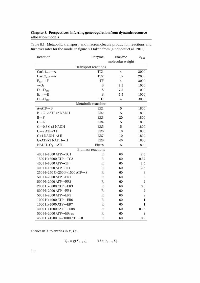
Chapter 8. Perspectives: inferring gene regulation from dynamic resourceallocation models
Table 8.1: Metabolic, transport, and macromolecule production reactions andturnover rates for the model in figure 8.1 taken from (Lindhorst et al., 2016).
Reaction Enzyme Enzyme kcat
molecular weight
Transport reactionsCarb1ext →A TC1 4 3000Carb2ext →A TC2 15 2000Fext →F TF 4 3000→O2 S 7.5 1000D→Dext S 7.5 1000Eext ↔E S 7.5 1000H→Hext TH 4 3000
Metabolic reactionsA+ATP→B ER1 5 1800B→C+2 ATP+2 NADH ER2 5 1800B→F ER3 20 1800C→G ER4 5 1800G→0.8 C+2 NADH ER5 5 1800C↔2 ATP+3 D ER6 10 1800C+4 NADH→3 E ER7 10 1800G+ATP+2 NADH↔H ER8 40 1800NADH+O2 →ATP ERres 5 1800
Biomass reactions400 H+1600 ATP→TC1 R 60 2.51500 H+6000 ATP→TC2 R 60 0.67400 H+1600 ATP→TF R 60 2.5400 H+1600 ATP→TH R 60 2.5250 H+250 C+250 F+1500 ATP→S R 60 3500 H+2000 ATP→ER1 R 60 2500 H+2000 ATP→ER2 R 60 22000 H+8000 ATP→ER3 R 60 0.5500 H+2000 ATP→ER4 R 60 2500 H+2000 ATP→ER5 R 60 21000 H+4000 ATP→ER6 R 60 11000 H+4000 ATP→ER7 R 60 14000 H+16000 ATP→ER8 R 60 0.25500 H+2000 ATP→ERres R 60 24500 H+1500 C+21000 ATP→R R 60 0.2
entries in X to entries in Y , i.e.
Yi∗ = g (Xi−1 ∗), ∀i ∈ {2, . . . ,K }.
162

8.2 The simplest case: a linear model
0 10 20 30 40 50time
0
20
40
60
80
100
exte
rnal m
eta
bolit
e a
mounts Carb1
extCarb2
ext
Dext
Eext
Fext
Hext
Figure 8.2: Extracellular metabolite time courses for the deFBA model in ta-ble 8.1, showing the diauxic shift under aerobic conditions.
Note that we use the enzyme production fluxes and not the enzyme amountsbecause the latter only increase in a deFBA model, while the fluxes can increaseand decrease and thus mimic up- and downregulation.
8.2 The simplest case: a linear modelWhile in general regulatory interactions are nonlinear and best described by sig-moid functions (see (Jamshidi, 2012) and references therein), we discuss herethe most simple possible case and assume g to be a linear function, i.e.
Yi∗ = g (Xi−1 ∗) := M Xi−1 ∗+εi , ∀i ∈ {2, . . . ,K }, (8.1)
where ε denotes the error terms, i.e., the difference between the predicted en-zyme production fluxes vRE and the actual enzyme production fluxes Y used astraining and obtained from the resource allocation model,
ε := Y − vRE = Y −M X .
The matrix M , which can also be seen as the adjacency matrix of a regulatorynetwork, then gives the influences of extracellular metabolite amounts on en-zyme synthesis fluxes, with positive entries upregulating the production of thecorresponding enzymes and negative entries downregulating it.
In statistics, the task of learning M is called multiple linear regression and isone of the simplest machine learning tools (Friedman et al., 2001). The methodfinds, for the system in equation 8.1, a matrix M such that the square error εᵀε isminimized (thus the name least squares regression).
One important property we would like to have for M is sparsity. This comesfrom two motivations: it is unlikely that any component has more than three
163

Chapter 8. Perspectives: inferring gene regulation from dynamic resourceallocation models
regulators due to crowding effects, and the more edges the regulatory networkhas the more we are prone to overfitting the data.
Shrinkage methods such as Ridge or Lasso regression minimize the regressioncoefficients in M by imposing a penalty on their size. This is done by introducingan additional term in the objective which penalizes either the 2- (in the case ofRidge) or the 1-norm (in the case of Lasso) of the coefficients using a Lagrangemultiplier parameter λ. Thus, the objectives of Ridge and Lasso regression forthe system in equation 8.1 are
minM
εᵀε−λ||M ||p ,
with p = 2 and p = 1 respectively. A third shrinkage method, the elastic net, usesboth the 1- and 2-norm penalties in the objective.
Such shrinkage methods are the easiest way of obtaining sparsity in the resultingnetwork M . Thus, we use least squares, Ridge, Lasso, and elastic net regressionfor estimating the regulation network in this section.
We use as training data time courses of the toy deFBA model in figure 8.1 with theinitial extracellular metabolite amounts in table 8.2 under aerobic conditions.We infer the four linear models using the python package scikit-learn (http://scikit-learn.org/stable/index.html).
Table 8.2: Initial extracellular metabolite amounts for the deFBA model to gen-erate the training data. The deFBA problems were solved using the final timet f = 70 with N = 70 discretization points for the dynamic variables.
Condition Carb1ext Carb2ext Dext Eext Fext Hext
1 2 120 0 0 0 02 10 110 0 0 0 03 20 100 0 0 0 04 30 90 0 0 0 05 40 80 0 0 0 06 50 70 0 0 0 07 60 60 0 0 0 08 70 50 0 0 0 09 80 40 0 0 0 010 90 30 0 0 0 011 100 20 0 0 0 012 110 10 0 0 0 013 120 2 0 0 0 0
After training the linear models we obtain four matrices, MLS, MLasso, MRidge,and MEN , which describe the influences of extracellular metabolite levels on en-zyme production fluxes. We show the values in MLS, MLasso, MRidge, and MEN in
164

8.3 Evaluating the learned regulation
tables A11-A14 in Appendix E. We note that, in the case of the shrinkage meth-ods, the influences of the Lagrange multiplier values on the results vary, with theLasso being the most sensitive to the values of λ and the Ridge being the leastsensitive. We have chosen the values in such a way that the smallest regressioncoefficients are used, while at the same time ensuring a good prediction behav-ior, as we will see next.
8.3 Evaluating the learned regulation
After learning the regulation, we would like to know how close the system thatincludes regulation is to the original deFBA time courses. We expect a lowergrowth rate, since deFBA shows us the behavior of the system assuming an idealregulatory system, i.e., assuming the error ε in equation (8.1) is zero.
To evaluate our learned regulation, we have developed an iterative procedurewhere at each time point the learned regulation is applied to determine the tar-get enzyme production fluxes vRE . Then, a linear program (LPreg) is used to ob-tain a solution that is as close as possible to these target synthesis fluxes, whileobeying a steady-state for the internal metabolite amounts, irreversibilities, andenzyme capacity constraints.
Note that vRE (ti+1) is a prediction of the new target fluxes given the extracellularmetabolite amounts nX (ti ). vRE (ti+1) is different from the training data Y .
We start by presenting the algorithm to compute such an iterative regulationenzyme-cost solution:
Algorithm 1 Algorithm to compute an iterative regulation enzyme-cost solution.
Input: vector n(t0) of initial enzyme and external metabolite amounts,learned function g s.t. vRE (ti+1) = g (nX (ti )), step size ∆t , end time t f .
i := 0while ti < t f do
ti+1 := ti +∆t .Compute target enzyme production fluxes vRE (ti+1) := g (nX (ti )).Find v(ti+1) from vRE (ti+1) and n(ti ) using (LPreg).if ∃v(ti+1) then
Compute new amounts n(ti+1) = n(ti )+Sv(ti+1)∆t .else
Break.end ifi := i +1.
end whileReturn n(t ),v(t )∀t ∈ {t1, . . . , ti−1}
If the organism cannot grow in the given environment using the resources in
165

Chapter 8. Perspectives: inferring gene regulation from dynamic resourceallocation models
n(t0), then Algorithm 1 will return infeasible. If this is not the case, then Algo-rithm 1 will run either until it has reached the given end time t f , or until it is notpossible to find a new flux vector using (LPreg) because the extracellular nutri-ents are exhausted.
To compute enzyme production fluxes that are as close as possible to the targetfluxes vRE (ti+1) given the resource allocation model, the enzyme and extracel-lular metabolite amounts n(ti ), and the step size∆t we solve the following linearprogram:
maxγ(ti+1)∈R,v(ti+1)∈R|R|
γ(ti+1)
s.t. γ(ti+1) · vRE (ti+1) ≤ vRE (ti+1)
SM∗v(ti+1) = 0∑i∈νk
vi (ti+1)
k i+cat
≤ nk (ti ) ∀k ∈ E
− ∑i∈νk \Irr
vi (ti+1)
k i−cat
≤ nk (ti ) ∀k ∈ E (LPreg)
nX (ti )−SX∗v(ti+1)∆t ≥ 0
vIrr(ti+1) ≥ 0
The linear program (LPreg) computes a flux vector vRE (ti+1) such that internalmetabolites are kept at steady-state, enzyme capacity constraints are obeyed,no more external metabolite amounts are used than available in the given stepsize, and irreversible reactions only go forward. This flux vector is the vectorthat contains the enzyme production fluxes closest to the target values vRE (ti+1)obtained by applying the regulation function, and at the same time maximizesgrowth by maximizing the enzyme production fluxes.
The (LPreg) is solved at each iteration of Algorithm 1 and for each of these iter-ations a different γ(ti+1) is computed. The role of γ(ti+1) in (LPreg) is to bringvRE (ti+1) as close as possible to vRE (ti+1). Moreover, a closer look at (LPreg) willreveal that, by maximizing γ(ti+1), we implicitly maximize vRE (ti+1) and hencewe also maximize biomass production.
Other ways that could be used to bring vRE (ti+1) as close as possible to vRE (ti+1)would be minimizing the 1-, 2- or infinity-norm of their difference as
minv(ti+1)∈R|R|
∣∣∣∣vRE (ti+1)− vRE (ti+1)∣∣∣∣
c ,
with c ∈ {1,2,∞} and eliminating the constraint involving γ(ti+1). We have triedthese objective functions as well, but the resulting time course predictions wereworse than when using the γ formulation in (LPreg).
Since the function g representing the regulation was learned from the timecourses of an optimal resource allocation model, by being as close as possible
166
8.3 Evaluating the learned regulation
to the values predicted by g , we are as close as possible to the optimal resourceallocation, while at the same time taking into account the regulatory part.We note that this iterative scheme is setting a different objective function ateach step by allowing a different γ(ti+1) and requiring different target enzymesynthesis fluxes at each time point.
We have applied Algorithm 1 for the four linear models MLS , MLasso , MRi d g e ,and ME N to evaluate how close the iterative regulation enzyme-cost solutionis to the deFBA solution. We show the resulting dynamics of enzyme synthesisfluxes and extracellular metabolite amounts in figures 8.3 and 8.4, respectively.
We observe that in all four cases there is a significant delay in the time coursesof the iterative regulation enzyme-cost solution compared to the deFBA timecourses. However, the overall qualitative behavior is strikingly similar, suggest-ing that the linear predictors are a good model.
On the other hand, the matrices MLS, MLasso, MRidge, and MEN are far fromsparse or intuitive. They all display a negative influence of Carb1ext on the pro-duction of the transporter for Carb2ext , which is why we do see preferential up-take of Carb1ext in figure 8.4 for all four models. However, this connection comesalong with other influences in MLS, MLasso, MRidge, and MEN which are hard tounderstand.
167

0 50 100 150 2000
2
4
610-4 ER1
0 50 100 150 2000
2
4
610-4 ER2
0 50 100 150 2000
2
410-4 ER3
0 50 100 150 2000
0.5
1
1.510-3 ER4
0 50 100 150 2000
0.5
1
1.510-3 ER5
0 50 100 150 2000
2
4
610-4 ER6
0 50 100 150 2000
2
4
610-8 ER7
0 50 100 150 2000
2
410-4 ER8
0 50 100 150 2000
1
210-3 ERres
0 50 100 150 2000
1
2
310-4 ETC1
0 50 100 150 2000
0.5
1
1.510-3 ETC2
0 50 100 150 200-1
0
1ETH
0 50 100 150 200-1
0
1ETF
enzy
me s
ynth
esi
s fluxe
s
0 50 100 150 2000
0.005
0.01
0.015S
0 50 100 150 2000
2
4
610-4 RIB
deFBAleast squaresLassoRidgeelastic net
time
x x
xx
xx
x x
xx
x
x
Figure 8.3: Evaluation of the learned linear regulation models. Shown are the enzyme synthesis time courses for the deFBA modelusing cCarb1ext
(0) = 120, cCarb2ext(0) = 100, cDext
(0) = cEext(0) = cFext
(0) = cHext(0) = 0 as initial conditions (continuous curves), and
the time courses obtained using the iterative enzyme-cost regulation in Algorithm 1 for the different linear models (dotted curves).

0 50 100 150 200time
0
20
40
60
80
100
120
extr
ace
llula
r m
eta
bolit
e a
mounts
least squares
0 50 100 150 200time
0
20
40
60
80
100
120
extr
ace
llula
r m
eta
bolit
e a
mounts
Lasso
0 50 100 150 200time
0
20
40
60
80
100
120
extr
ace
llula
r m
eta
bolit
e a
mounts
Ridge
0 50 100 150 200time
0
20
40
60
80
100
120
extr
ace
llula
r m
eta
bolit
e a
mounts
elastic net
Carb1ext
Carb2ext
Dext
Figure 8.4: Evaluation of the learned linear regulation models. Shown are the extracellular metabolite time courses for the deFBAmodel using cCarb1ext
(0) = 120, cCarb2ext(0) = 100, cDext
(0) = cEext(0) = cFext
(0) = cHext(0) = 0 as initial conditions (continuous curves),
and the time courses obtained using the iterative enzyme-cost regulation in Algorithm 1 for the different linear models (dottedcurves).

Chapter 8. Perspectives: inferring gene regulation from dynamic resourceallocation models
8.4 Discussion
This chapter presented some first steps in the direction of inferring regulatorystructures using time courses from dynamic resource allocation models. Wehave seen that it is possible to infer matrices that implement the regulationresponsible for diauxie using simple machine learning tools such as linear re-gression. Moreover, we have presented here an iterative algorithm that appliesthe learned regulation while taking into account enzyme capacity constraints.The benefit of this iterative procedure compared to deFBA is that, when makingthe prediction for the current time point, the model no longer has knowledge ofwhat will happen in the future.
We have seen that, although we only used linear models, we can rediscover thegeneral shape of the enzyme synthesis time courses predicted by deFBA. In ad-dition, although we observe a lag period compared to deFBA, the extracellularmetabolite time courses resulting from this procedure display the preferentialuse of one carbon source over the alternative.
However, the inferred matrices are hard to interpret and do not necessarily re-flect the general structure of regulation networks encountered in biology. Whatwe would expect to see is rather a sparse network with three layers: an inputlayer consisting of extracellular metabolite time courses and exchange reactionfluxes which then influence a middle layer of transcription factors, which thenin turn influence an “output” layer, namely the enzyme synthesis fluxes. Thisresembles more the structure of another very popular machine learning tool: anartificial neural network with one hidden layer which represents the transcrip-tion factors.
We are thus tempted to assume that, if we were to use a neural network instead ofa linear regression model, we might be able to get even closer to the deFBA timecourses than we are in figures 8.3 and 8.4. By using a logistic activation functionfor the middle layer, we would be even closer to the sigmoid shape of activationand inhibition used in ODE models of gene regulatory networks (Klipp et al.,2008).
On the other hand, this can come at several expenses. First, we would needmuch more training data than we have used in this perspectives chapter. Sec-ond, we would be fitting more parameters and we would be in more danger ofoverfitting our data. Third, finding global optima when inferring neural net-works is hard since we are no longer in the well-studied linear case, but we areactually fitting nonlinear functions. Last, there would always be the questions ofhow large should the hidden layer be, what values should we use for the initialguess, how should we ensure sparsity?
It may be helpful to already enforce some regulatory links to be present in thenetwork, based on prior knowledge that we can obtain from databases such asYeastract (Teixeira et al., 2014). This is not trivial since it comes at the expense of
170

8.4 Discussion
having to implement the solving routine to incorporate additional constraintson neural network edges.
An important extension to the iterative scheme and the learning procedurewould also be to include the enzyme amounts and the import fluxes fornonlimiting extracellular metabolites as explanatory variables in the inferenceproblem. An example would be, for the toy model in figure 8.1, the import fluxfor oxygen. Since oxygen is not assumed to be limiting, its extracellular amountis not modeled, but only the import flux. Thus, for learning regulatory mech-anisms responsible for oxygen shifts of the type in chapter 7, it is important toallow connections between the oxygen import flux and the enzyme synthesisfluxes.
171


Chapter 9
Conclusions
This PhD thesis is dedicated to the study of dynamic resource allocation inmetabolic networks. In the beginning of my PhD studies the state of the artin this topic was limited to the existence of two related methods: dynamicenzyme-cost flux balance analysis (Waldherr et al., 2015) and conditional fluxbalance analysis (Rügen et al., 2015). These methods had been applied, as aproof of concept, to a small core carbon network adapted from (Covert et al.,2001) and to a minimal model of phototrophic growth, respectively. In addition,there were two related formalisms for steady-state resource allocation studies:resource balance analysis (Goelzer et al., 2011) and gene expression models(Lerman et al., 2012). These had already been successfully applied at genomescale for the study of Bacillus subtilis, Thermatoga maritima, and Escherichiacoli.
However, there were no guidelines for how to construct a dynamic genome-scaleresource allocation model. Thus, my first contribution was to find the ingredi-ents of such models, how they come together and depend on each other, whatare the units of each ingredient, and where to find all the data needed to buildsuch a model. This is now formulated as a guide and presented in chapter 4.In addition to this guide, chapter 4 also provides a standard for encoding suchmodels in SBML, for ease of exchange and reproducibility.
When I started this PhD there was also no software prototype for solving dy-namic resource allocation problems at genome-scale. While implementing thissoftware I had to tackle all the mathematical difficulties presented in chapter 5.This started with solution dependencies on simulation end point, and contin-ued with numerical discretization of the dynamic variables and problem re-formulation, giving upper bounds on the model-derived growth rates, suitablyscaling the resulting linear programs, analyzing the convexity of the quadrati-cally constrained cFBA problem and thus justifying that binary search is a suit-able solving approach, and ending with the actual software implementation andsolver interfaces.
173

Chapter 9. Conclusions
All the results in chapter 5 made it possible to study dynamic resource allocationat genome-scale for the first time. This was done in two case studies, on Syne-chococcus elongatus in chapter 6, and on Saccharomyces cerevisiae in chapter 7.
The case study on Synechococcus elongatus pinpointed several energetic trade-offs and constraints related to diurnal growth in cyanobacteria. Among the keyresults was the observation that growth is dynamic and takes place during thelight phase. This was shown to be an optimal behavior that arises as a trade-off between the cost of not using existing enzymes and ribosomes during darkand the additional storage costs that would be required to continue using theseenzymatic resources at night. Moreover, the linear pattern of glycogen accu-mulation throughout the day was shown to be an optimal behavior. The closematch between the model-derived and experimental growth rates pointed outthat cyanobacterial metabolism operates close to optimality.
The study of dynamic resource allocation in Saccharomyces cerevisiae subjectedto environmental changes showed that two seemingly suboptimal behaviorsthat are widely spread in nature, overflow metabolism and diauxie, are in factconsequences of an optimal allocation of enzyme resources. Moreover, wehave discovered that, in case of oxygen availability fluctuations, a key propertythat allows some of the individuals to survive is their ability to rewire theirmetabolism and to restore their NAD+/NADH redox balance. Finally, we haveshown that the experimentally observed increasing growth rate lag that arisesupon a nutrient shift after increasing time feeding on the preferred carbonsource is due to the time yeast needs to synthesize the large and numerousrespiratory and TCA cycle enzymes needed to grow optimally on the alternatecarbon source.
The natural next steps would be to use the time courses resulting from these dy-namic resource allocation studies to infer the regulatory structures that coordi-nate the observed optimal behaviors. Chapter 8 provided some preliminary re-sults in this direction using machine learning and an iterative regulation schemecombined with resource allocation. I believe that this idea has a lot of potentialand that more effort should be dedicated to alternative inference tools besideslinear models, with the natural next choice being neural networks.
Finally, another point where resource allocation studies may provide further un-derstanding of biology are microbial community interactions. In such a mi-crobial community, the species cooperate by exchanging metabolites and thisway grow faster than if they would not cross-feed. However, as pointed out in(Gottstein et al., 2016), existing approaches either fail to predict the interactionsin the first place as is the case for FBA, or easily become computationally in-tractable due to the nonlinear kinetic description of the exchange fluxes, as isthe case for dynamic FBA. One of the main challenges arising in such commu-nity models is also modeling organisms that grow at different rates, but still co-operate and survive together. I argue that, in the end, the cooperative behavior
174

is due to sharing resources and that dynamic resource allocation studies usingdeFBA may provide solutions to the challenges encountered so far.
175

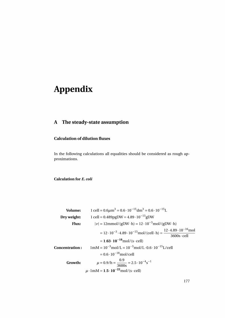
Appendix
A The steady-state assumption
Calculation of dilution fluxes
In the following calculations all equalities should be considered as rough ap-proximations.
Calculation for E. coli
Volume: 1 cell = 0.6µm3 = 0.6 ·10−15dm3 = 0.6 ·10−15L
Dry weight: 1 cell = 0.489pgDW = 4.89 ·10−13gDW
Flux: |v | = 12mmol/(gDW ·h) = 12 ·10−3mol/(gDW ·h)
= 12 ·10−3 ·4.89 ·10−13mol/(cell ·h) = 12 ·4.89 ·10−16mol
3600s ·cell= 1.63 ·10−18mol/(s ·cell)
Concentration : 1mM = 10−3mol/L = 10−3mol/L ·0.6 ·10−15L/cell
= 0.6 ·10−18mol/cell
Growth: µ= 0.9/h = 0.9
3600s= 2.5 ·10−4s−1
µ ·1mM = 1.5 ·10−22mol/(s ·cell)
177

Calculation for S. cerevisiae
Volume: 1 cell = 20µm3 = 2 ·10−14L
Dry weight: 1 cell = 10−11gDW
Flux: |v | = 0.5mmol/(h ·gDW) = 0.5 ·10−3mol/(h ·gDW)
= 0.5 ·10−3 ·10−11mol/h = 0.5 ·10−3 ·10−11mol
3600s ·cell= 1.38 ·10−18mol/(s ·cell)
Concentration : 1mM = 10−3mol/L = 10−3mol/L ·2 ·10−14L/cell
= 2 ·10−17mol/cell
Growth: µ= 0.4/h = 0.4
3600s= 1.11 ·10−4s−1
µ ·1mM = 2.22 ·10−21mol/(s ·cell)
Calculation for H. sapiens (HeLa)
Volume: 1 cell = 2600µm3 = 2.6 ·10−12L
Protein weight: 1 cell = 150pgProtein = 1.5 ·10−7mgProtein
Flux: v = 18nmol/(min ·mgProtein) = 18 ·10−9mol/(min ·mgProtein)
= 18 ·10−9 ·1.5 ·10−7mol/(min ·cell) = 18 ·10−9 ·1.5 ·10−7mol
60s ·cell= 4.5 ·10−17mol/(s ·cell)
Concentration : 1mM = 10−3mol/L = 10−3mol/L ·2.6 ·10−12L/cell
= 2.6 ·10−15mol/cell
Growth: µ= 0.06/h = 0.06
3600s= 1.67 ·10−5s−1
µ ·1mM = 4.34 ·10−20mol/(s ·cell)
178
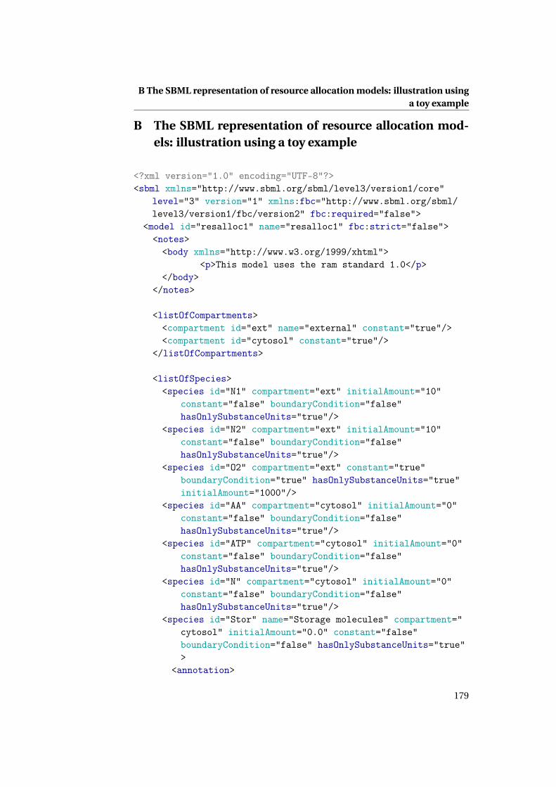
B The SBML representation of resource allocation models: illustration usinga toy example
B The SBML representation of resource allocation mod-els: illustration using a toy example
<?xml version="1.0" encoding="UTF-8"?><sbml xmlns="http://www.sbml.org/sbml/level3/version1/core"
level="3" version="1" xmlns:fbc="http://www.sbml.org/sbml/level3/version1/fbc/version2" fbc:required="false">
<model id="resalloc1" name="resalloc1" fbc:strict="false"><notes><body xmlns="http://www.w3.org/1999/xhtml">
<p>This model uses the ram standard 1.0</p></body>
</notes>
<listOfCompartments><compartment id="ext" name="external" constant="true"/><compartment id="cytosol" constant="true"/>
</listOfCompartments>
<listOfSpecies><species id="N1" compartment="ext" initialAmount="10"
constant="false" boundaryCondition="false"hasOnlySubstanceUnits="true"/>
<species id="N2" compartment="ext" initialAmount="10"constant="false" boundaryCondition="false"hasOnlySubstanceUnits="true"/>
<species id="O2" compartment="ext" constant="true"boundaryCondition="true" hasOnlySubstanceUnits="true"initialAmount="1000"/>
<species id="AA" compartment="cytosol" initialAmount="0"constant="false" boundaryCondition="false"hasOnlySubstanceUnits="true"/>
<species id="ATP" compartment="cytosol" initialAmount="0"constant="false" boundaryCondition="false"hasOnlySubstanceUnits="true"/>
<species id="N" compartment="cytosol" initialAmount="0"constant="false" boundaryCondition="false"hasOnlySubstanceUnits="true"/>
<species id="Stor" name="Storage molecules" compartment="cytosol" initialAmount="0.0" constant="false"boundaryCondition="false" hasOnlySubstanceUnits="true">
<annotation>
179

<ram:RAM xmlns:ram="https://www.fairdomhub.org/sops/304">
<ram:species ram:molecularWeight="weight_0" ram:objectiveWeight="zero" ram:biomassPercentage="zero" ram:speciesType="storage"/>
</ram:RAM></annotation>
</species><species id="Complex_1" name="Transporter complex"
compartment="cytosol" initialAmount="0.004166667083123639" constant="false"boundaryCondition="false" hasOnlySubstanceUnits="true">
<annotation><ram:RAM xmlns:ram="https://www.fairdomhub.org/sops
/304"><ram:species ram:molecularWeight="weight_1" ram:
objectiveWeight="weight_11" ram:biomassPercentage="zero" ram:speciesType="enzyme"/>
</ram:RAM></annotation>
</species><species id="Emetab1" name="Generic metabolic enzyme"
compartment="cytosol" initialAmount="1.9442790116926745" constant="false" boundaryCondition="false" hasOnlySubstanceUnits="true">
<annotation><ram:RAM xmlns:ram="https://www.fairdomhub.org/sops
/304"><ram:species ram:molecularWeight="weight_2" ram:
objectiveWeight="weight_12" ram:biomassPercentage="zero" ram:speciesType="enzyme"/>
</ram:RAM></annotation>
</species><species id="Emetab2" name="Specialized metabolic enzyme"
compartment="cytosol" initialAmount="0.008000000399798693" constant="false"boundaryCondition="false" hasOnlySubstanceUnits="true">
<annotation><ram:RAM xmlns:ram="https://www.fairdomhub.org/sops
/304">
180

B The SBML representation of resource allocation models: illustration usinga toy example
<ram:species ram:molecularWeight="weight_3" ram:objectiveWeight="weight_13" ram:biomassPercentage="zero" ram:speciesType="enzyme"/>
</ram:RAM></annotation>
</species><species id="Estor" name="Metabolic enzyme for handling
storage" compartment="cytosol" initialAmount="0.0"constant="false" boundaryCondition="false"hasOnlySubstanceUnits="true">
<annotation><ram:RAM xmlns:ram="https://www.fairdomhub.org/sops
/304"><ram:species ram:molecularWeight="weight_4" ram:
objectiveWeight="weight_14" ram:biomassPercentage="zero" ram:speciesType="enzyme"/>
</ram:RAM></annotation>
</species><species id="Etrans1" name="Transporter enzyme"
compartment="cytosol" initialAmount="0.005555555555555556" constant="false"boundaryCondition="false" hasOnlySubstanceUnits="true">
<annotation><ram:RAM xmlns:ram="https://www.fairdomhub.org/sops
/304"><ram:species ram:molecularWeight="weight_5" ram:
objectiveWeight="weight_15" ram:biomassPercentage="zero" ram:speciesType="enzyme"/>
</ram:RAM></annotation>
</species><species id="Etrans2" name="Cofactor of transporter enzyme
" compartment="cytosol" initialAmount="0.0" constant="false" boundaryCondition="false" hasOnlySubstanceUnits="true">
<annotation><ram:RAM xmlns:ram="https://www.fairdomhub.org/sops
/304"><ram:species ram:molecularWeight="weight_6" ram:
objectiveWeight="weight_16" ram:biomassPercentage="zero" ram:speciesType="enzyme"/>
</ram:RAM>
181

</annotation></species><species id="R" name="Ribosome" compartment="cytosol"
initialAmount="0.033641975308641964" constant="false"boundaryCondition="false" hasOnlySubstanceUnits="true">
<annotation><ram:RAM xmlns:ram="https://www.fairdomhub.org/sops
/304"><ram:species ram:molecularWeight="weight_7" ram:
objectiveWeight="weight_17" ram:biomassPercentage="zero" ram:speciesType="enzyme"/>
</ram:RAM></annotation>
</species><species id="S" name="Structrual biomass component"
compartment="cytosol" initialAmount="0.7499999999999999" constant="false" boundaryCondition="false" hasOnlySubstanceUnits="true">
<annotation><ram:RAM xmlns:ram="https://www.fairdomhub.org/sops
/304"><ram:species ram:molecularWeight="weight_8" ram:
objectiveWeight="weight_18" ram:biomassPercentage="biomp" ram:speciesType="quota"/>
</ram:RAM></annotation>
</species></listOfSpecies>
<listOfParameters><parameter constant="true" id="kcatt" value="1800" /><parameter constant="true" id="kcatC" value="2400" /><parameter constant="true" id="kcat1" value="2000" /><parameter constant="true" id="kcat2" value="2500" /><parameter constant="true" id="zero" value="0.0" /><parameter constant="true" id="kcatR1" value="10" /><parameter constant="true" id="kcatR2" value="16.67" /><parameter constant="true" id="kcatR3" value="5" /><parameter constant="true" id="kcatR4" value="6.25" /><parameter constant="true" id="kcatR5" value="1" /><parameter constant="true" id="kcatR6" value="10" /><parameter constant="true" id="kcatC1" value="6.25" /><parameter constant="true" id="kcatSf" value="25" />
182

B The SBML representation of resource allocation models: illustration usinga toy example
<parameter constant="true" id="kcatSb" value="30" /><parameter constant="true" id="main" value="0.2" /><parameter constant="true" id="biomp" value="0.15" /><parameter constant="true" id="weight_0" value="0.2" /><parameter constant="true" id="weight_1" value="0.16" /><parameter constant="true" id="weight_2" value="0.2" /><parameter constant="true" id="weight_3" value="0.16" /><parameter constant="true" id="weight_4" value="0.15" /><parameter constant="true" id="weight_5" value="0.1" /><parameter constant="true" id="weight_6" value="0.06" /><parameter constant="true" id="weight_7" value="1.0" /><parameter constant="true" id="weight_8" value="1.5" /><parameter constant="true" id="weight_10" value="0.2" /><parameter constant="true" id="weight_11" value="0.16" /><parameter constant="true" id="weight_12" value="0.2" /><parameter constant="true" id="weight_13" value="0.16" /><parameter constant="true" id="weight_14" value="0.15" /><parameter constant="true" id="weight_15" value="0.1" /><parameter constant="true" id="weight_16" value="0.06" /><parameter constant="true" id="weight_17" value="1.0" /><parameter constant="true" id="weight_18" value="1.5" />
</listOfParameters>
<fbc:listOfGeneProducts><fbc:geneProduct fbc:id="Etrans1" fbc:label="1*GTRANS1"
fbc:associatedSpecies="Etrans1"/><fbc:geneProduct fbc:id="Etrans2" fbc:label="1*GTRANS2"
fbc:associatedSpecies="Etrans2"/><fbc:geneProduct fbc:id="Complex_1" fbc:label="1*GTRANS1
AND 1*GTRANS2" fbc:associatedSpecies="Complex_1" /><fbc:geneProduct fbc:id="Emetab1" fbc:label="1*GMETAB1"
fbc:associatedSpecies="Emetab1"/><fbc:geneProduct fbc:id="Emetab2" fbc:label="1*GMETAB2"
fbc:associatedSpecies="Emetab2"/><fbc:geneProduct fbc:id="R" fbc:label="1*GRIBOS" fbc:
associatedSpecies="R"/><fbc:geneProduct fbc:id="Estor" fbc:label="1*GSTORF" fbc:
associatedSpecies="Estor"/></fbc:listOfGeneProducts>
<listOfReactions><reaction id="Maintenance" reversible="false" fast="true"><annotation>
183

<ram:RAM xmlns:ram="https://www.fairdomhub.org/sops/304">
<ram:reaction ram:kcatForward="zero" ram:kcatBackward="zero" ram:maintenanceScaling="main"/>
</ram:RAM></annotation><listOfReactants><speciesReference species="AA" stoichiometry="50"
constant="true"/><speciesReference species="ATP" stoichiometry="60"
constant="true"/></listOfReactants>
</reaction><reaction id="PMetab1" reversible="false" fast="false"><annotation><ram:RAM xmlns:ram="https://www.fairdomhub.org/sops
/304"><ram:reaction ram:kcatForward="kcatR3" ram:
kcatBackward="zero" ram:maintenanceScaling="zero"/>
</ram:RAM></annotation><fbc:geneProductAssociation fbc:id="Ribosome">
<fbc:geneProductRef fbc:geneProduct="R" /></fbc:geneProductAssociation><listOfReactants><speciesReference species="AA" stoichiometry="200"
constant="true"/><speciesReference species="ATP" stoichiometry="800"
constant="true"/></listOfReactants><listOfProducts><speciesReference species="Emetab1" stoichiometry="1"
constant="true"/></listOfProducts>
</reaction><reaction id="Metab1_1" reversible="false" fast="true"><annotation><ram:RAM xmlns:ram="https://www.fairdomhub.org/sops
/304"><ram:reaction ram:kcatForward="kcat1" ram:
kcatBackward="zero" ram:maintenanceScaling="zero"/>
184

B The SBML representation of resource allocation models: illustration usinga toy example
</ram:RAM></annotation><fbc:geneProductAssociation fbc:id="Emetab1">
<fbc:geneProductRef fbc:geneProduct="Emetab1" /></fbc:geneProductAssociation><listOfReactants><speciesReference species="N" stoichiometry="1"
constant="true"/></listOfReactants><listOfProducts><speciesReference species="AA" stoichiometry="1"
constant="true"/><speciesReference species="ATP" stoichiometry="1"
constant="true"/></listOfProducts>
</reaction><reaction id="Trans2" reversible="true" fast="false"><annotation><ram:RAM xmlns:ram="https://www.fairdomhub.org/sops
/304"><ram:reaction ram:kcatForward="kcatC" ram:
kcatBackward="kcatC" ram:maintenanceScaling="zero"/>
</ram:RAM></annotation><fbc:geneProductAssociation fbc:id="Complex_1"><fbc:geneProductRef fbc:geneProduct="Complex_1"/>
</fbc:geneProductAssociation><listOfReactants><speciesReference species="N2" stoichiometry="1"
constant="true"/></listOfReactants><listOfProducts><speciesReference species="N" stoichiometry="1"
constant="true"/></listOfProducts>
</reaction><reaction id="Metab1_2" reversible="false" fast="true"><annotation><ram:RAM xmlns:ram="https://www.fairdomhub.org/sops
/304"><ram:reaction ram:kcatForward="kcat2" ram:
kcatBackward="zero" ram:maintenanceScaling="zero"/>
185

</ram:RAM></annotation><fbc:geneProductAssociation fbc:id="Emetab2">
<fbc:geneProductRef fbc:geneProduct="Emetab2" /></fbc:geneProductAssociation><listOfReactants><speciesReference species="N" stoichiometry="1"
constant="true"/></listOfReactants><listOfProducts><speciesReference species="AA" stoichiometry="1"
constant="true"/><speciesReference species="ATP" stoichiometry="1"
constant="true"/></listOfProducts>
</reaction><reaction id="Trans1" reversible="true" fast="false"><annotation><ram:RAM xmlns:ram="https://www.fairdomhub.org/sops
/304"><ram:reaction ram:kcatForward="kcatt" ram:
kcatBackward="kcatt" ram:maintenanceScaling="zero"/>
</ram:RAM></annotation><fbc:geneProductAssociation fbc:id="Etrans1"><fbc:geneProductRef fbc:geneProduct="Etrans1" />
</fbc:geneProductAssociation><listOfReactants><speciesReference species="N1" stoichiometry="1"
constant="true"/><speciesReference species="O2" stoichiometry="2"
constant="true"/></listOfReactants><listOfProducts><speciesReference species="N" stoichiometry="1"
constant="true"/></listOfProducts>
</reaction><reaction id="Storing" reversible="true" fast="false" fbc:
lowerFluxBound="kcatSf" fbc:upperFluxBound="kcatSb"><annotation><ram:RAM xmlns:ram="https://www.fairdomhub.org/sops
/304">
186

B The SBML representation of resource allocation models: illustration usinga toy example
<ram:reaction ram:kcatForward="kcatSf" ram:kcatBackward="kcatSb" ram:maintenanceScaling="zero"/>
</ram:RAM></annotation><fbc:geneProductAssociation fbc:id="Estor"><fbc:geneProductRef fbc:geneProduct="Estor" />
</fbc:geneProductAssociation><listOfReactants><speciesReference species="AA" stoichiometry="200"
constant="true"/><speciesReference species="ATP" stoichiometry="
300" constant="true"/></listOfReactants><listOfProducts><speciesReference species="Stor" stoichiometry="1"
constant="true"/></listOfProducts>
</reaction><reaction id="PEtrans1" reversible="false" fast="false"><annotation><ram:RAM xmlns:ram="https://www.fairdomhub.org/sops
/304"><ram:reaction ram:kcatForward="kcatR1" ram:
kcatBackward="zero" ram:maintenanceScaling="zero"/>
</ram:RAM></annotation><fbc:geneProductAssociation fbc:id="Ribosome">
<fbc:geneProductRef fbc:geneProduct="R" /></fbc:geneProductAssociation><listOfReactants><speciesReference species="AA" stoichiometry="100"
constant="true"/><speciesReference species="ATP" stoichiometry="400"
constant="true"/></listOfReactants><listOfProducts><speciesReference species="Etrans1" stoichiometry="1"
constant="true"/></listOfProducts>
</reaction><reaction id="PEtrans2" reversible="false" fast="false"><annotation>
187
<ram:RAM xmlns:ram="https://www.fairdomhub.org/sops/304">
<ram:reaction ram:kcatForward="kcatR2" ram:kcatBackward="zero" ram:maintenanceScaling="zero"/>
</ram:RAM></annotation><fbc:geneProductAssociation fbc:id="Ribosome">
<fbc:geneProductRef fbc:geneProduct="R" /></fbc:geneProductAssociation><listOfReactants><speciesReference species="AA" stoichiometry="60"
constant="true"/><speciesReference species="ATP" stoichiometry="240"
constant="true"/></listOfReactants><listOfProducts><speciesReference species="Etrans2" stoichiometry="1"
constant="true"/></listOfProducts>
</reaction><reaction id="PComplex_1" reversible="false" fast="false"><annotation><ram:RAM xmlns:ram="https://www.fairdomhub.org/sops
/304"><ram:reaction ram:kcatForward="kcatC1" ram:
kcatBackward="zero" ram:maintenanceScaling="zero"/>
</ram:RAM></annotation><fbc:geneProductAssociation fbc:id="Ribosome">
<fbc:geneProductRef fbc:geneProduct="R" /></fbc:geneProductAssociation><listOfReactants><speciesReference species="AA" stoichiometry="160"
constant="true"/><speciesReference species="ATP" stoichiometry="640"
constant="true"/></listOfReactants><listOfProducts><speciesReference species="Complex_1" stoichiometry="1
" constant="true"/></listOfProducts>
</reaction>
188

B The SBML representation of resource allocation models: illustration usinga toy example
<reaction id="PMetab2" reversible="false" fast="false"><annotation><ram:RAM xmlns:ram="https://www.fairdomhub.org/sops
/304"><ram:reaction ram:kcatForward="kcatR4" ram:
kcatBackward="zero" ram:maintenanceScaling="zero"/>
</ram:RAM></annotation><fbc:geneProductAssociation fbc:id="Ribosome">
<fbc:geneProductRef fbc:geneProduct="R" /></fbc:geneProductAssociation><listOfReactants><speciesReference species="AA" stoichiometry="160"
constant="true"/><speciesReference species="ATP" stoichiometry="640"
constant="true"/></listOfReactants><listOfProducts><speciesReference species="Emetab2" stoichiometry="1"
constant="true"/></listOfProducts>
</reaction><reaction id="PEstor" reversible="false" fast="false"><annotation><ram:RAM xmlns:ram="https://www.fairdomhub.org/sops
/304"><ram:reaction ram:kcatForward="kcatR3" ram:
kcatBackward="zero" ram:maintenanceScaling="zero"/>
</ram:RAM></annotation><fbc:geneProductAssociation fbc:id="Ribosome">
<fbc:geneProductRef fbc:geneProduct="R" /></fbc:geneProductAssociation><listOfReactants><speciesReference species="AA" stoichiometry="150"
constant="true"/><speciesReference species="ATP" stoichiometry="600"
constant="true"/></listOfReactants><listOfProducts><speciesReference species="Estor" stoichiometry="1"
constant="true"/>
189

</listOfProducts></reaction><reaction id="PR" name="Ribosome expression" reversible="
false" fast="false"><annotation><ram:RAM xmlns:ram="https://www.fairdomhub.org/sops
/304"><ram:reaction ram:kcatForward="kcatR5" ram:
kcatBackward="zero" ram:maintenanceScaling="zero"/>
</ram:RAM></annotation><fbc:geneProductAssociation fbc:id="Ribosome">
<fbc:geneProductRef fbc:geneProduct="R" /></fbc:geneProductAssociation><listOfReactants><speciesReference species="AA" stoichiometry="1000"
constant="true"/><speciesReference species="ATP" stoichiometry="4000"
constant="true"/></listOfReactants><listOfProducts><speciesReference species="R" stoichiometry="1"
constant="true"/></listOfProducts>
</reaction><reaction id="Metab2" reversible="false" fast="true"><annotation><ram:RAM xmlns:ram="https://www.fairdomhub.org/sops
/304"><ram:reaction ram:kcatForward="kcat1" ram:
kcatBackward="zero" ram:maintenanceScaling="zero"/>
</ram:RAM></annotation><fbc:geneProductAssociation fbc:id="Emetab2">
<fbc:geneProductRef fbc:geneProduct="Emetab2" /></fbc:geneProductAssociation><listOfReactants><speciesReference species="N" stoichiometry="1"
constant="true"/></listOfReactants><listOfProducts>
190

B The SBML representation of resource allocation models: illustration usinga toy example
<speciesReference species="AA" stoichiometry="1"constant="true"/>
<speciesReference species="ATP" stoichiometry="2"constant="true"/>
</listOfProducts></reaction><reaction id="PS" name="Structural biomass production"
reversible="false" fast="false"><annotation><ram:RAM xmlns:ram="https://www.fairdomhub.org/sops
/304"><ram:reaction ram:kcatForward="kcatR6" ram:
kcatBackward="zero" ram:maintenanceScaling="zero"/>
</ram:RAM></annotation>
<fbc:geneProductAssociation fbc:id="Ribosome"><fbc:geneProductRef fbc:geneProduct="R" />
</fbc:geneProductAssociation><listOfReactants><speciesReference species="AA" stoichiometry="1500"
constant="true"/><speciesReference species="ATP" stoichiometry="200"
constant="true"/></listOfReactants><listOfProducts><speciesReference species="S" stoichiometry="1"
constant="true"/></listOfProducts>
</reaction></listOfReactions>
</model></sbml>
191

C Synechococcus elongatus 7942 model
Table A1: Ribosome composition of S. elongatus 7942.
Ribosomal Gene Stoichiometry Molecularprotein weight (Da)
Small ribosomal subunitS1 Synpcc7942_0694 1 34591S2 Synpcc7942_2530 1 28400S3 Synpcc7942_2226 1 27718S4 Synpcc7942_1487 1 23206S5 Synpcc7942_2216 1 19330S6 Synpcc7942_0012 1 12346S7 Synpcc7942_0886 1 17756S8 Synpcc7942_2219 1 14682S9 Synpcc7942_2205 1 14937S10 Synpcc7942_0883 1 12179S11 Synpcc7942_2210 1 13712S12 Synpcc7942_0887 1 13991S13 Synpcc7942_2211 1 13979S14 Synpcc7942_0446 1 11752S15 Synpcc7942_2299 1 10308S16 Synpcc7942_1772 1 9555S17 Synpcc7942_2223 1 9347S18 Synpcc7942_1123 1 8307S19 Synpcc7942_2228 1 10238S20 Synpcc7942_1520 1 10892S21 Synpcc7942_1774 1 7029
Large ribosomal subunitL1 Synpcc7942_0633 1 25855L2 Synpcc7942_2229 1 31706L3 Synpcc7942_2232 1 22452L4 Synpcc7942_2231 1 23203L5 Synpcc7942_2220 1 20016L6 Synpcc7942_2218 1 19198L7/L12 Synpcc7942_0631 2x (2-3)=4-6 13151L9 Synpcc7942_2559 1 16679L10 Synpcc7942_0632 1 18810L11 Synpcc7942_0634 1 14903L13 Synpcc7942_2206 1 17072L14 Synpcc7942_2222 1 13318L15 Synpcc7942_2215 1 15289L16 Synpcc7942_2225 1 16139
Continued on next page
192

C Synechococcus elongatus 7942 model
Table A1 – continued from previous pageRibosomal Gene Stoichiometry Molecularprotein weight (Da)L17 Synpcc7942_2208 1 13262L18 Synpcc7942_2217 1 13047L19 Synpcc7942_2541 1 13444L20 Synpcc7942_1277 1 13316L21 Synpcc7942_1219 1 13870L22 Synpcc7942_2227 1 13253L23 Synpcc7942_2230 1 11148L24 Synpcc7942_2221 1 12449L27 Synpcc7942_1220 1 9227L28 Synpcc7942_0042 1 9119L29 Synpcc7942_2224 1 7650L31 Synpcc7942_2204 1 8799L32 Synpcc7942_0997 1 6534L33 Synpcc7942_1122 1 7372L34 Synpcc7942_1614 1 5230L35 Synpcc7942_1278 1 7840L36 Synpcc7942_2212 1 4364
Ribosomal RNA16S Synpcc7942_R0004 15S Synpcc7942_R0006 123S Synpcc7942_R0005 1
Table A2: Gene composition of the photosystems I and II monomers of S. elon-gatus 7942.
Enzyme Gene Gene name Stoichiometry
Photosystem I Synpcc7942_2049 PsaA 1monomer Synpcc7942_2048 PsaB 1
Synpcc7942_0535 PsaC 1Synpcc7942_1002 PsaD 1Synpcc7942_1322 PsaE 1Synpcc7942_1250 PsaF 1Synpcc7942_2343 PsaI 1Synpcc7942_1249 PsaJ 1Synpcc7942_0407 PsaK1 (PsaX) 1Synpcc7942_0920 (PsaK2) (PsaX) 1Synpcc7942_2342 PsaL 1Synpcc7942_1912a PsaM 1C05306_cyt Chlorophyll a 96
Continued on next page
193

Table A2 – continued from previous pageEnzyme Gene Gene name Stoichiometry
C02094_cyt µ-carotene 22C02059_cyt Phylloquinone 2
Photosystem II Synpcc7942_0424 (A) 1monomer Synpcc7942_0893 (A) 1
Synpcc7942_1389 (A) 1Synpcc7942_0655 (D1) PsbA (D1) 1Synpcc7942_1637 (D2) PsbD (D2) 1Synpcc7942_0697 PsbB 1Synpcc7942_0656 PsbC 1Synpcc7942_1177 PsbE 1Synpcc7942_1176 PsbF 1Synpcc7942_0225 PsbH 1Synpcc7942_1705 PsbI 1Synpcc7942_1174 PsbJ 1Synpcc7942_0456 PsbK 1Synpcc7942_1175 PsbL 1Synpcc7942_0699 PsbM 1Synpcc7942_0224 PsbN 1Synpcc7942_0294 PsbO 1Synpcc7942_1038 PspP 1Synpcc7942_0696 PsbT 1Synpcc7942_1882 PsbU 1Synpcc7942_2010 PsbV 1Synpcc7942_2016 PsbX 1Synpcc7942_1692 PsbY 1Synpcc7942_2245 PsbZ 1Synpcc7942_0343 Psb27 1Synpcc7942_1679 Psb28 (W) 1Synpcc7942_2478 Psb28-2 (W) 1C05306_cyt Chlorophyll a 35C02094_cyt µ-carotene 11
194

C Synechococcus elongatus 7942 model
Table A3: Gene composition of phycobilisomes in S. elongatus 7942. The follow-ing abbreviations are used: α PC - Phycocyanin alpha subunit, µ PC - Phyco-cyanin beta subunit, α AP - Allophycocyanin alpha subunit, µ AP - Allophyco-cyanin beta subunit, Lcr - core-rod linker protein, Lr - rod-rod linker protein, Lc- core-core linker protein, Lcm - core-thylakoid membrane linker protein.
Subunit Description Gene or Gene Stoichiometrymetabolite name
Core24 · (αAP+µAP)
Phycocyanobilin 48Synpcc7942_0327 ApcA 24Synpcc7942_0326 ApcB 24
6 ·Lc Synpcc7942_0325 ApcC 62 ·Lcm Synpcc7942_0328 ApcE 2
Rods(length 1)
+36 · (αPC+µPC)Phycocyanobilin +108Synpcc7942_1048 CpcA +36Synpcc7942_1047 CpcB +36
+6 ·Lcr Synpcc7942_2030 CpcG +6
Rods(length 2)
+36 · (αPC+µPC)Phycocyanobilin +108Synpcc7942_1048 CpcA +36Synpcc7942_1047 CpcB +36
+6 ·Lr Synpcc7942_1049 CpcC +6
Rods(length 3)
+36 · (αPC+µPC)Phycocyanobilin +108Synpcc7942_1048 CpcA +36Synpcc7942_1047 CpcB +36
+6 ·Lr Synpcc7942_1049 CpcC +6
Table A4: Gene composition of NDH I, Cytochrome b6f, ATPase, Cytochrome coxidase, and succinate dehydrogenase.
Enzyme Gene Gene name Stoichiometry
NADPH dehydrogenase Core (State M):Synpcc7942_1343 NdhA 1Synpcc7942_1415 NdhB 1Synpcc7942_1180 NdhC 1Synpcc7942_1346 NdhE 1Synpcc7942_1345 NdhG 1Synpcc7942_1743 NdhH 1Synpcc7942_1344 NdhI 1Synpcc7942_1182 NdhJ 1Synpcc7942_1181 NdhK 1Synpcc7942_0413 NdhL 1Synpcc7942_1982 NdhM 1
Continued on next page
195

Table A4 – continued from previous pageEnzyme Gene Gene name Stoichiometry
Synpcc7942_2234 NdhN 1Synpcc7942_2177 NdhO 1Variable:
State L:Synpcc7942_1976 NdhD1 1Synpcc7942_1977 NdhF1 1
State L’:Synpcc7942_1439 NdhD2 1Synpcc7942_1977 NdhF1 1
State MS:Synpcc7942_2092 NdhD3 1Synpcc7942_2091 NdhF3 1Synpcc7942_2093 CupA 1Synpcc7942_2094 CupS 1
State MS’:Synpcc7942_0609 NdhD4 1Synpcc7942_0309 NdhF4 1Synpcc7942_0308 CupB 1
Cytochrome b6f Synpcc7942_1232 PetC 2Synpcc7942_2426 PetM 2Synpcc7942_0978 PetH (FNR) 2Synpcc7942_1231 PetA 2Synpcc7942_2331 PetB 2Synpcc7942_2332 PetD 2Synpcc7942_0475 PetN 2Synpcc7942_1479 PetG 2Synpcc7942_0113 PetL 2Cytochrome:Synpcc7942_0239 cyt f 1Synpcc7942_1630 cyt A (Pet J) 1Synpcc7942_2542 Cyt c6-2 1
ATPase Synpcc7942_0331 A 1Synpcc7942_0332 C 10-15Synpcc7942_0333 B’ 1-2Synpcc7942_0334 B 1-2Synpcc7942_0335 delta 1Synpcc7942_0336 alpha 3Synpcc7942_0337 gamma 1Synpcc7942_2315 beta 3Synpcc7942_2316 epsilon 1
Continued on next page
196

C Synechococcus elongatus 7942 model
Table A4 – continued from previous pageEnzyme Gene Gene name Stoichiometry
Cytochrome c oxidase Synpcc7942_2603 sub I 1Synpcc7942_2602 subII 1Synpcc7942_2604 sub III 1
Succinate dehydrogenase Synpcc7942_0314 SdhC 1Synpcc7942_0641 SdhA 1Synpcc7942_1533 SdhB 1
Table A5: Fractions of the dry weight of a S. elongatus cell that correspond to thequota metabolites as well as absolute amounts of the quota metabolites in onecell, assuming a dry weight of 1.5 pg/cell.
quota metabolite fraction (g/gDW) Amount (pg/cell)
Noncatalytic proteins 0.357 0.5712DNA 0.031 0.0496RNA 0.17 0.272Cell wall 0.059 0.0944Lipids 0.12 0.192Cofactors and vitamins 0.029 0.0464Ions 0.01 0.016Pigments 0.0244 0.03904
197

D Saccharomyces cerevisiae model
Table A6: Verduyn minimal medium composition and corresponding Yeast 6transporters.
Compound Transporters
D-glucose r_1714D-galactose r_1710oxygen r_1992(NH4)2SO4 r_1654, r_2060, r_2061KH2PO4 r_2020, r_2005MgSO4 ·7H2O r_2060, r_2061D-biotin r_1671Ca-D-pantothenate r_1548Nicotonic acid r_1967Myo-inositol r_1947Thiamine hydrochloride r_2067Pyridoxal hydrochloride r_2028p-aminobenzoic acid r_1604Na2 r_2049ZnSO4 ·7H2O r_2060, r_2061MnCl2 ·2H2O -CoCl2 ·6H2O -CuSO4 ·5H2O r_2060, r_2061Na2MoO4 ·2H2O -CaCl2 ·2H2O -FeSO4 ·7H2O r_1861H3BO3 -KI -
Table A7: Additional medium components needed for anaerobic growth, andtheir corresponding Yeast 6 transporters.
Compound Transporters
episterol r_1753ergosterol r_1757fecosterol r_1788lanosterol r_1915zymosterol r_210614-demethyllanosterol r_2134ergosta-5,7,22,24(28)-tetraen-3beta-ol r_2137oleate r_2189
198

D Saccharomyces cerevisiae model
Table A8: Ribosome composition of S. cerevisiae. All gene stoichiometries are 1.
Ribosomal protein Gene name Gene
Small ribosomal subunit
SARPS0A YGR214WRPS0B YLR048W
S2 RPS2 YGL123WS3 RPS3 YNL178W
S3ARPS1A YLR441CRPS1B YML063W
S4RPS4A YJR145CRPS4B YHR203C
S5 RPS5 YJR123W
S6RPS6A YPL090CRPS6B YBR181C
S7RPS7A YOR096WRPS7B YNL096C
S8RPS8A YBL072CRPS8B YER102W
S9RPS9A YPL081WRPS9B YBR189W
S10RPS10A YOR293WRPS10B YMR230W
S11RPS11A YDR025WRPS11B YBR048W
S12 RPS12 YOR369CS13 RPS13 YDR064W
S14RPS14A YCR031CRPS14B YJL191W
S15 RPS15 YOL040C
S15ARPS22A YJL190CRPS22B YLR367W
S16RPS16A YMR143WRPS16B YDL083C
S17RPS17A YML024WRPS17B YDR447C
S18RPS18A YDR450WRPS18B YML026C
S19RPS19A YOL121CRPS19B YNL302C
S20 RPS20 YHL015WS21 RPS21A YKR057W
Continued on next page
199

Table A8 – continued from previous pageRibosomal protein Gene name GeneS21 RPS21B YJL136C
S23RPS23A YGR118WRPS23B YPR132W
S24RPS24A YER074WRPS24B YIL069C
S25RPS25A YGR027CRPS25B YLR333C
S26RPS26A YGL189CRPS26B YER131W
S27RPS27A YKL156WRPS27B YHR021C
S27A RPS31 YLR167W
S28RPS28A YOR167CRPS28B YLR264W
S29RPS29A YLR388WRPS29B YDL061C
S30RPS30A YLR287C-ARPS30B YOR182C
Large ribosomal subunitLP0 RPP0 YLR340W
LP1RPP1A YDL081CRPP1B YDL130W
LP2 RPP2A YOL039WL3 RPL3 YOR063W
L4RPL4A YBR031WRPL4B YDR012W
L5 RPL5 YPL131W
L6RPL6A YML073CRPL6B YLR448W
L7RPL7A YGL076CRPL7B YPL198W
L7ARPL8A YHL033CRPL8B YLL045C
L8RPL2A YFR031C-ARPL2B YIL018W
L9RPL9A YGL147CRPL9B YNL067W
L10 RPL10 YLR075W
L10ARPL1A YPL220WRPL1B YGL135W
Continued on next page
200

D Saccharomyces cerevisiae model
Table A8 – continued from previous pageRibosomal protein Gene name Gene
L11RPL11A YPR102CRPL11B YGR085C
L12RPL12A YEL054CRPL12B YDR418W
L13RPL13A YDL082WRPL13B YMR142C
L13ARPL16A YIL133CRPL16B YNL069C
L14RPL14A YKL006WRPL14B YHL001W
L15RPL15A YLR029CRPL15B YMR121C
L17RPL17A YKL180WRPL17B YJL177W
L18RPL18A YOL120CRPL18B YNL301C
L18ARPL20A YMR242CRPL20B YOR312C
L19RPL19A YBR084C-ARPL19B YBL027W
L21RPL21A YBR191WRPL21B YPL079W
L22RPL22A YLR061WRPL22B YFL034C-A
L23RPL23A YBL087CRPL23B YER117W
L23A RPL25 YOL127W
L24RPL24A YGL031CRPL24B YGR148C
L26RPL26A YLR344WRPL26B YGR034W
L27RPL27A YHR010WRPL27B YDR471W
L27A RPL28 YGL103WL29 RPL29 YFR032C-AL30 RPL30 YGL030W
L31RPL31A YDL075WRPL31B YLR406C
L32 RPL32 YBL092WL34 RPL34A YER056C-A
Continued on next page
201

Table A8 – continued from previous pageRibosomal protein Gene name GeneL34 RPL34B YIL052C
L35RPL35A YDL191WRPL35B YDL136W
L35ARPL33A YPL143WRPL33B YOR234C
L36RPL36A YMR194WRPL36B YPL249C-A
L36ARPL42A YNL162WRPL42B YHR141C
L37RPL37A YLR185WRPL37B YDR500C
L37ARPL43A YPR043WRPL43B YJR094W-A
L38 RPL38 YLR325CL39 RPL39 YJL189W
L40RPL40A YIL148WRPL40B YKR094C
L41RPL41A YDL184CRPL41B YDL133C-A
Ribosomal RNA25S RDN25-15S RDN5-15.8S RDN58-118S RDN18-1
202

DSa
ccha
romyces
cerevisiae
mo
del
Table A9: Quota metabolite production reactions for S. cerevisiae. The reactions and energy requirements have been constructedfollowing the information in the supplement of (Förster et al., 2003a).
Reactants Stoichiometry Products Stoichiometry
Nocatalytic proteinsAla-tRNA(Ala) 0.9839201541 tRNA(Ala) 0.9839201541Arg-tRNA(Arg) 0.3446294001 tRNA(Arg) 0.3446294001Asn-tRNA(Asn) 0.2181008711 tRNA(Asn) 0.2181008711Asp-tRNA(Asp) 0.6380040232 tRNA(Asp) 0.6380040232Cys-tRNA(Cys) 0.0141540388 tRNA(Cys) 0.0141540388Gln-tRNA(Gln) 0.2260357111 tRNA(Gln) 0.2260357111Glu-tRNA(Glu) 0.6472255939 tRNA(Glu) 0.6472255939Gly-tRNA(Gly) 0.6227777087 tRNA(Gly) 0.6227777087His-tRNA(His) 0.1421837537 tRNA(His) 0.1421837537Ile-tRNA(Ile) 0.4132550429 tRNA(Ile) 0.4132550429Leu-tRNA(Leu) 0.6356450167 tRNA(Leu) 0.6356450167Lys-tRNA(Lys) 0.6137705931 tRNA(Lys) 0.6137705931Met-tRNA(Met) 0.1087287529 tRNA(Met) 0.1087287529Phe-tRNA(Phe) 0.2871554242 tRNA(Phe) 0.2871554242Pro-tRNA(Pro) 0.3532076054 tRNA(Pro) 0.3532076054Ser-tRNA(Ser) 0.3975998181 tRNA(Ser) 0.3975998181Thr-tRNA(Thr) 0.4104671262 tRNA(Thr) 0.4104671262Trp-tRNA(Trp) 0.060905258 tRNA(Trp) 0.060905258Tyr-tRNA(Tyr) 0.2187442365 tRNA(Tyr) 0.2187442365Val-tRNA(Val) 0.5674482841 tRNA(Val) 0.5674482841
Continued on next page
203

Table A9 – continued from previous pageReactants Stoichiometry Products StoichiometryATP 36.3823134562 ADP 36.3823134562H2O 36.3823134562 phosphate 36.3823134562
H+ 36.3823134562protein quota 1
RNAAMP 0.691255 RNA quota 1CMP 0.671719 ADP 24.614677GMP 0.691255 H+ 24.614677UMP 0.900134 phosphate 24.614677ATP 24.614677H2O 24.614677
DNAdAMP 0.919380 DNA quota 1dCMP 0.612920 ADP 26.559855dGMP 0.612920 H+ 26.559855dTMP 0.919380 phosphate 26.559855ATP 26.559855H2O 26.559855
Cell wall(1 → 3)-beta-D-glucan 3.605775 cell wall quota 1mannan 2.567065 ADP 16.553263ATP 16.553263 H+ 16.553263H2O 16.553263 phosphate 16.553263
Continued on next page
204

DSa
ccha
romyces
cerevisiae
mo
del
Table A9 – continued from previous pageReactants Stoichiometry Products Stoichiometry
Lipids1-phosphatidyl-1D-myo-inositol 0.185284 lipid quota 114-demethyllanosterol 0.006782complex sphingolipid 0.050499episterol 0.011626ergosta-5,7,22,24(28)-tetraen-3beta-ol 0.015138ergosterol 0.678165ergosterol ester 0.098334fatty acid 0.024947fecosterol 0.013806lanosterol 0.003875phosphatidyl-L-serine 0.045171phosphatidylcholine 0.348771phosphatidylethanolamine 0.084407triglyceride 0.094580zymosterol 0.001817
Small moleculesriboflavin 0.431599 small molecules quota 1sulphate 8.719170
205

Table A10: Fractions of the dry weight of a S. cerevisiae cell that correspond tothe quota metabolites.
quota metabolite fraction (g/gDW)
noncatalytic proteins 0.27731RNA 0.066546DNA 0.0039157cell wall 0.31472lipids 0.0082576small molecules 0.0022938
206

E Regulation inference using deFBA time courses
E Regulation inference using deFBA time courses
Table A11: Transpose of the least squares regression matrix MLS learned usingdeFBA time courses for the toy model in figure 8.1.
Carb1ext Carb2ext Dext Eext Fext Hext
ER1 0.00019381 0.00015021 0.0013658 -2.2705 0 0ER2 0.00021147 0.00018655 0.00060077 -2.8392 0 0ER3 -3.0439e-05 -5.0733e-05 0.00092267 -0.31313 0 0ER4 -5.193e-05 -7.3483e-05 0.0036452 4.0171 0 0ER5 -0.00016764 -0.00020332 0.0034676 5.6247 0 0ER6 1.9984e-05 -3.89e-05 0.00079994 -0.238 0 0ER7 -3.3693e-08 1.5392e-08 1.9897e-07 0.0037495 0 0ER8 9.6483e-05 9.1794e-05 0.0004666 -1.8497 0 0ERres -7.6346e-05 -0.00014287 0.0067211 1.9126 0 0ETC1 0.00021299 -1.8809e-06 0.00027752 -1.0494 0 0ETC2 -0.00025606 0.00016953 0.0016208 -2.6385 0 0ETH 0 0 0 0 0 0ETF 0 0 0 0 0 0S -0.003285 -0.0059422 0.079068 120.01 0 0RIB 0.00018009 0.00016234 0.0011605 -3.7149 0 0
Table A12: Transpose of the Lasso regression matrix MLasso (objective Lagrangemultiplier λ= 0.115) learned using deFBA time courses for the toy model in fig-ure 8.1.
Carb1ext Carb2ext Dext Eext Fext Hext
ER1 0.00017539 0.00016227 0.0011829 -0 0 0ER2 0.00019353 0.0001987 0.00041413 -0 0 0ER3 -0 -0 0.00067714 0 0 0ER4 -8.2981e-06 -2.4977e-06 0.0033939 0 0 0ER5 -0.00012543 -0.0001326 0.003227 0 0 0ER6 0 0 0.00059914 0 0 0ER7 0 0 0 0 0 0ER8 7.7699e-05 0.00010379 0.00028652 -0 0 0ERres -3.0924e-05 -7.156e-05 0.0064559 0 0 0ETC1 0.00019352 9.9853e-06 0.00010272 -0 0 0ETC2 -0.00018036 0.00015524 0.0014088 -0 0 0ETH 0 0 0 0 0 0ETF 0 0 0 0 0 0S -0.0033411 -0.005891 0.079585 0 0 0RIB 0.00016291 0.00017464 0.00096803 -0 0 0
207

Table A13: Transpose of the Ridge regression matrix MRi d g e (objective Lagrangemultiplier λ = 105) learned using deFBA time courses for the toy model in fig-ure 8.1.
Carb1ext Carb2ext Dext Eext Fext Hext
ER1 0.00020323 0.0001894 0.0011256 -1.4931e-08 0 0ER2 0.00021314 0.00020067 0.00049013 -2.4703e-08 0 0ER3 -2.004e-05 -2.0394e-05 0.0007607 1.9977e-09 0 0ER4 -1.6188e-05 4.2613e-05 0.0030387 5.9358e-08 0 0ER5 -0.00013163 -8.9192e-05 0.0028951 7.4231e-08 0 0ER6 2.7094e-05 -1.2239e-05 0.00066033 2.0254e-09 0 0ER7 -3.2894e-08 2.0771e-08 1.8546e-07 3.7875e-11 0 0ER8 9.9724e-05 0.00010398 0.00038026 -1.5652e-08 0 0ERres -7.1847e-06 7.1492e-05 0.0055727 5.5565e-08 0 0ETC1 0.0002077 9.3213e-06 0.00022628 -8.9323e-09 0 0ETC2 -0.00022469 0.00021064 0.0013308 -1.6804e-08 0 0ETH 0 0 0 0 0 0ETF 0 0 0 0 0 0S -0.0024955 -0.0032847 0.065934 1.6113e-06 0 0RIB 0.00018921 0.00019445 0.00094788 -3.0205e-08 0 0
Table A14: Transpose of the elastic net regression matrix ME N (objective La-grange multiplier λ = 0.2) learned using deFBA time courses for the toy modelin figure 8.1.
Carb1ext Carb2ext Dext Eext Fext Hext
ER1 0.00017805 0.00016078 0.0012046 -0 0 0ER2 0.00019619 0.00019719 0.00043595 -0 0 0ER3 -0 -0 0.00069879 0 0 0ER4 -1.4297e-05 -1.1814e-05 0.0034295 0 0 0ER5 -0.00013152 -0.00014183 0.0032626 0 0 0ER6 0 0 0.00062081 0 0 0ER7 0 0 0 0 0 0ER8 8.0358e-05 0.00010227 0.00030835 -0 0 0ERres -3.699e-05 -8.0672e-05 0.0064909 0 0 0ETC1 0.00019617 8.4662e-06 0.0001246 -0 0 0ETC2 -0.00018991 0.00015721 0.0014339 -0 0 0ETH 0 0 0 0 0 0ETF 0 0 0 0 0 0S -0.0033462 -0.0058973 0.079606 0 0 0RIB 0.00016557 0.00017315 0.00098974 -0 0 0
208

Bibliography
R. Aebersold and M. Mann. Mass spectrometry-based proteomics. Nature, 422(6928):198–207, 2003.
T. Aho, H. Almusa, J. Matilainen, A. Larjo, P. Ruusuvuori, K.-L. Aho, T. Wilhelm,H. Lähdesmäki, A. Beyer, M. Harju, et al. Reconstruction and validation ofRefRec: a global model for the yeast molecular interaction network. PLoS One,5(5):e10662, 2010.
E. Albers, C. Larsson, G. Lidén, C. Niklasson, and L. Gustafsson. Influence of thenitrogen source on Saccharomyces cerevisiae anaerobic growth and productformation. Applied and Environmental Microbiology, 62(9):3187–3195, 1996.
J. Almquist, M. Cvijovic, V. Hatzimanikatis, J. Nielsen, and M. Jirstrand. Kineticmodels in industrial biotechnology – improving cell factory performance.Metabolic Engineering, 24:38–60, 2014.
K. B. Andersen and K. von Meyenburg. Are growth rates of Escherichia coli inbatch cultures limited by respiration? Journal of Bacteriology, 144(1):114–123,1980.
S. Angermayr, P. van Alphen, D. Hasdemir, G. Kramer, M. Iqbal, W. van Gron-delle, H. Hoefsloot, Y. Choi, and K. Hellingwerf. Culturing Synechocystis sp.strain PCC 6803 with N2 and CO2 in a diel regime reveals multiphase glycogendynamics with low maintenance costs. Applied Environmental Microbiology,82(14):4180–4189, 2016.
R. Ansell, K. Granath, S. Hohmann, J. M. Thevelein, and L. Adler. The two isoen-zymes for yeast NAD+-dependent glycerol 3-phosphate dehydrogenase en-coded by GPD1 and GPD2 have distinct roles in osmoadaptation and redoxregulation. The EMBO Journal, 16(9):2179–2187, 1997.
M. Ataman, D. F. Hernandez Gardiol, G. Fengos, and V. Hatzimanikatis. redGEM:Systematic reduction and analysis of genome-scale metabolic reconstruc-tions for development of consistent core metabolic models. PLoS Compu-tational Biology, 13(7):1–22, 07 2017.
209
Bibliography
H. W. Aung, S. A. Henry, and L. P. Walker. Revising the representation of fatty acid,glycerolipid, and glycerophospholipid metabolism in the consensus model ofyeast metabolism. Industrial Biotechnology, 9(4):215–228, 2013.
B. M. Bakker, K. M. Overkamp, A. J. van Maris, P. Kötter, M. A. Luttik, J. P.van Dijken, and J. T. Pronk. Stoichiometry and compartmentation of NADHmetabolism in Saccharomyces cerevisiae. FEMS Microbiology Reviews, 25(1):15–37, 2001.
M. Bartl, P. Li, and S. Schuster. Modelling the optimal timing in metabolicpathway activation—use of pontryagin’s maximum principle and role of thegolden section. Biosystems, 101(1):67–77, 2010.
D. A. Beard, S. dan Liang, and H. Qian. Energy balance for analysis of complexmetabolic networks. Biophysical Journal, 83:79–86, 2002.
D. A. Beard, E. Babson, E. Curtis, and H. Qian. Thermodynamic constraints forbiochemical networks. Journal of Theoretical Biology, 228(3):327–333, 2004.
C. Beck, S. Hertel, A. Rediger, R. Lehmann, A. Wiegard, A. Kolsch, B. Heilmann,J. Georg, W. R. Hess, and I. M. Axmann. Daily expression pattern of protein-encoding genes and small noncoding RNAs in Synechocystis sp. strain PCC6803. Applied Environmental Microbiology, 80(17):5195–5206, 2014.
Q. K. Beg, A. Vazquez, J. Ernst, M. A. de Menezes, Z. Bar-Joseph, A.-L. Barabási,and Z. N. Oltvai. Intracellular crowding defines the mode and sequence ofsubstrate uptake by Escherichia coli and constrains its metabolic activity. Pro-ceedings of the National Academy of Sciences, 104(31):12663–12668, 2007.
J. Behre and S. Schuster. Modeling signal transduction in enzyme cascades withthe concept of elementary flux modes. Journal of Computational Biology, 16(6):829–844, 2009.
M. J. Behrenfeld, K. H. Halsey, and A. J. Milligan. Evolved physiological re-sponses of phytoplankton to their integrated growth environment. Philosoph-ical Transactions of the Royal Society B: Biological Sciences, 363(1504):2687–2703, 2008.
B. D. Bennett, E. H. Kimball, M. Gao, R. Osterhout, S. J. Van Dien, and J. D. Rabi-nowitz. Absolute metabolite concentrations and implied enzyme active siteoccupancy in Escherichia coli. Nature Chemical Biology, 5(8):593–599, 2009.
D. A. Benson, M. Cavanaugh, K. Clark, I. Karsch-Mizrachi, D. J. Lipman, J. Ostell,and E. W. Sayers. Genbank. Nucleic Acids Research, 41:D36–D42, 2013.
H. M. Berman, J. Westbrook, Z. Feng, G. Gilliland, T. N. Bhat, H. Weissig, I. N.Shindyalov, and P. E. Bourne. The Protein Data Bank. Nucleic Acids Research,28(1):235–242, 2000. doi: 10.1093/nar/28.1.235.
210

Bibliography
J. A. Bernstein, A. B. Khodursky, P.-H. Lin, S. Lin-Chao, and S. N. Cohen. Globalanalysis of mRNA decay and abundance in Escherichia coli at single-gene res-olution using two-color fluorescent DNA microarrays. Proceedings of the Na-tional Academy of Sciences, 99(15):9697–9702, 2002.
R. P. Bhalerao, T. Gillbro, and P. Gustafsson. Functional phycobilisome corestructures in a phycocyanin-less mutant of cyanobacterium Synechococcus sp.PCC 7942. Photosynthesis Research, 45(1):61–70, 1995.
E. Boles, P. de Jong-Gubbels, and J. T. Pronk. Identification and characterizationof MAE1, the Saccharomyces cerevisiae structural gene encoding mitochon-drial malic enzyme. Journal of Bacteriology, 180(11):2875–2882, 1998.
A. Bordbar, J. M. Monk, Z. A. King, and B. Ø. Palsson. Constraint-based modelspredict metabolic and associated cellular functions. Nature Reviews Genetics,15(2):107–120, 2014.
H. Bremer and P. Dennis. Modulation of chemical composition and other pa-rameters of the cell at different exponential growth rates. EcoSal Plus, 3(1),2008.
G. C. Brown. Total cell protein concentration as an evolutionary constraint onthe metabolic control distribution in cells. Journal of theoretical biology, 153(2):195–203, 1991.
F. Büchel, N. Rodriguez, N. Swainston, C. Wrzodek, T. Czauderna, R. Keller,F. Mittag, M. Schubert, M. Glont, M. Golebiewski, M. van Iersel, S. Keating,M. Rall, M. Wybrow, H. Hermjakob, M. Hucka, D. B. Kell, W. Müller, P. Mendes,A. Zell, C. Chaouiya, J. Saez-Rodriguez, F. Schreiber, C. Laibe, A. Dräger, andN. Le Novère. Path2Models: large-scale generation of computational modelsfrom biochemical pathway maps. BMC Systems Biology, 7(1):116, 2013.
A. P. Burgard, P. Pharkya, and C. D. Maranas. OptKnock: a bilevel programmingframework for identifying gene knockout strategies for microbial strain opti-mization. Biotechnology and Bioengineering, 84(6):647–657, 2003.
A. P. Burgard, E. V. Nikolaev, C. H. Schilling, and C. D. Maranas. Flux couplinganalysis of genome-scale metabolic network reconstructions. Genome re-search, 14(2):301–312, 2004.
R. L. Burnap. Systems and photosystems: cellular limits of autotrophic produc-tivity in cyanobacteria. Frontiers in Bioengineering and Biotechnology, 3:1,2015.
D. Campbell, V. Hurry, A. K. Clarke, P. Gustafsson, and G. Öquist. Chlorophyllfluorescence analysis of cyanobacterial photosynthesis and acclimation. Mi-crobiology and Molecular Biology Reviews, 62(3):667–683, 1998.
211

Bibliography
A. B. Canelas, W. M. van Gulik, and J. J. Heijnen. Determination of the cytoso-lic free NAD/NADH ratio in Saccharomyces cerevisiae under steady-state andhighly dynamic conditions. Biotechnology and Bioengineering, 100(4):734–743, 2008.
M. Celton, A. Goelzer, C. Camarasa, V. Fromion, and S. Dequin. A constraint-based model analysis of the metabolic consequences of increased NADPHoxidation in Saccharomyces cerevisiae. Metabolic Engineering, 14(4):366–379,2012.
V. Chelliah, N. Juty, I. Ajmera, R. Ali, M. Dumousseau, M. Glont, M. Hucka,G. Jalowicki, S. Keating, V. Knight-Schrijver, A. Lloret-Villas, K. Nath Natarajan,J.-B. Pettit, N. Rodriguez, M. Schubert, S. M. Wimalaratne, Y. Zhao, H. Herm-jakob, N. Le Novère, and C. Laibe. BioModels: ten-year anniversary. NucleicAcids Research, 43(D1):D542–D548, 2015.
J. M. Cherry, E. L. Hong, C. Amundsen, R. Balakrishnan, G. Binkley, E. T. Chan,K. R. Christie, M. C. Costanzo, S. S. Dwight, S. R. Engel, D. G. Fisk, J. E.Hirschman, B. C. Hitz, K. Karra, C. J. Krieger, S. R. Miyasato, R. S. Nash, J. Park,M. S. Skrzypek, M. Simison, S. Weng, and E. D. Wong. Saccharomyces GenomeDatabase: the genomics resource of budding yeast. Nucleic Acids Research, 30(D1):D700–D705, 2012.
C. Y. M. Cheung, M. G. Poolman, D. A. Fell, R. G. Ratcliffe, and L. J. Sweet-love. A diel flux balance model captures interactions between light and darkmetabolism during day-night cycles in C3 and crassulacean acid metabolismleaves. Plant Physiology, 165(2):917–929, 2014.
J. W. Cooley and W. F. Vermaas. Succinate dehydrogenase and other respiratorypathways in thylakoid membranes of Synechocystis sp. strain PCC 6803: ca-pacity comparisons and physiological function. Journal of Bacteriology, 183(14):4251–4258, 2001.
R. Costenoble, P. Picotti, L. Reiter, R. Stallmach, M. Heinemann, U. Sauer, andR. Aebersold. Comprehensive quantitative analysis of central carbon andamino-acid metabolism in Saccharomyces cerevisiae under multiple condi-tions by targeted proteomics. Molecular Systems Biology, 7(1):464, 2011.
M. W. Covert, C. H. Schilling, and B. Ø. Palsson. Regulation of gene expressionin flux balance models of metabolism. Journal of Theoretical Biology, 213(1):73–88, 2001.
D. Davidi, E. Noor, W. Liebermeister, A. Bar-Even, A. Flamholz, K. Tummler,U. Barenholz, M. Goldenfeld, T. Shlomi, and R. Milo. Global characteriza-tion of in vivo enzyme catalytic rates and their correspondence to in vitrokcat measurements. Proceedings of the National Academy of Sciences, 113(12):3401–3406, 2016.
212

Bibliography
L. M. De Godoy, J. V. Olsen, J. Cox, M. L. Nielsen, N. C. Hubner, F. Fröhlich, T. C.Walther, and M. Mann. Comprehensive mass-spectrometry-based proteomequantification of haploid versus diploid yeast. Nature, 455(7217):1251–1254,2008.
G. M. de Hijas-Liste, E. Klipp, E. Balsa-Canto, and J. R. Banga. Global dynamicoptimization approach to predict activation in metabolic pathways. BMC sys-tems biology, 8(1):1, 2014.
P. Deuflhard and F. Bornemann. Gewöhnliche Differentialgleichungen. Walter deGruyter, 2013.
D. Deutscher, I. Meilijson, M. Kupiec, and E. Ruppin. Multiple knockout analysisof genetic robustness in the yeast metabolic network. Nature Genetics, 38(9):993–998, 2006.
J. Deutscher. The mechanisms of carbon catabolite repression in bacteria. Cur-rent Opinion in Microbiology, 11(2):87–93, 2008.
S. Devoid, R. Overbeek, M. DeJongh, V. Vonstein, A. A. Best, and C. Henry. Auto-mated genome annotation and metabolic model reconstruction in the SEEDand Model SEED. Systems Metabolic Engineering: Methods and Protocols,pages 17–45, 2013.
S. Diamond, D. Jun, B. E. Rubin, and S. S. Golden. The circadian oscillatorin Synechococcus elongatus controls metabolite partitioning during diurnalgrowth. Proceedings of the National Academy of Sciences, 112(15):E1916–E1925, 2015.
P. D. Dobson, K. Smallbone, D. Jameson, E. Simeonidis, K. Lanthaler, P. Pir, C. Lu,N. Swainston, W. B. Dunn, P. Fisher, et al. Further developments towards agenome-scale metabolic model of yeast. BMC Systems Biology, 4(1):145, 2010.
M. M. dos Santos, V. Raghevendran, P. Kötter, L. Olsson, and J. Nielsen. Manip-ulation of malic enzyme in Saccharomyces cerevisiae for increasing NADPHproduction capacity aerobically in different cellular compartments. MetabolicEngineering, 6(4):352–363, 2004.
N. C. Duarte, M. J. Herrgård, and B. Ø. Palsson. Reconstruction and validationof Saccharomyces cerevisiae iND750, a fully compartmentalized genome-scalemetabolic model. Genome Research, 14(7):1298–1309, 2004.
J. S. Edwards, R. U. Ibarra, and B. Ø. Palsson. In silico predictions of Escherichiacoli metabolic capabilities are consistent with experimental data. NatureBiotechnology, 19(2):125–130, 2001.
M. B. Elowitz and S. Leibler. A synthetic oscillatory network of transcriptionalregulators. Nature, 403(6767):335–338, 2000.
213

Bibliography
P. Erdrich, H. Knoop, R. Steuer, and S. Klamt. Cyanobacterial biofuels: new in-sights and strain design strategies revealed by computational modeling. Mi-crobial Cell Factories, 13(1):128, 2014.
P. Erdrich, R. Steuer, and S. Klamt. An algorithm for the reduction of genome-scale metabolic network models to meaningful core models. BMC SystemsBiology, 9(1):48, 2015.
A. M. Feist, C. S. Henry, J. L. Reed, M. Krummenacker, A. R. Joyce, P. D. Karp, L. J.Broadbelt, V. Hatzimanikatis, and B. Ø. Palsson. A genome-scale metabolicreconstruction for Escherichia coli K-12 MG1655 that accounts for 1260 ORFsand thermodynamic information. Molecular Systems Biology, 3(1), 2007.
D. Fell. Understanding the control of metabolism. Portland Press London, 1997.
S.-M. Fendt and U. Sauer. Transcriptional regulation of respiration in yeast me-tabolizing differently repressive carbon substrates. BMC Systems Biology, 4(1):12, 2010.
A. Finka and P. Goloubinoff. Proteomic data from human cell cultures refinemechanisms of chaperone-mediated protein homeostasis. Cell Stress andChaperones, 18(5):591–605, 2013.
E. Fischer and U. Sauer. Large-scale in vivo flux analysis shows rigidity and sub-optimal performance of Bacillus subtilis metabolism. Nature Genetics, 37(6):636–640, 2005.
A. Flamholz, E. Noor, A. Bar-Even, and R. Milo. eQuilibrator-the biochemicalthermodynamics calculator. Nucleic Acids Research, 40(D1):D770–D775, 2012.
A. Flamholz, E. Noor, A. Bar-Even, W. Liebermeister, and R. Milo. Glycolytic strat-egy as a tradeoff between energy yield and protein cost. Proceedings of theNational Academy of Sciences, 110(24):10039–10044, 2013.
J. Förster, I. Famili, P. Fu, B. Ø. Palsson, and J. Nielsen. Genome-scale reconstruc-tion of the Saccharomyces cerevisiae metabolic network. Genome Research, 13(2):244–253, 2003a.
J. Förster, I. Famili, B. Ø. Palsson, and J. Nielsen. Large-scale evaluation of in sil-ico gene deletions in Saccharomyces cerevisiae. OMICS A Journal of IntegrativeBiology, 7(2):193–202, 2003b.
C. Francke, R. J. Siezen, and B. Teusink. Reconstructing the metabolic network ofa bacterium from its genome. Trends in Microbiology, 13(11):550–558, 2005.
J. Friedman, T. Hastie, and R. Tibshirani. The elements of statistical learning,volume 1 of Springer Series in Statistics. Springer, Berlin, 2001.
214

Bibliography
A. M. Gleixner, D. E. Steffy, and K. Wolter. Improving the Accuracy of LinearProgramming Solvers with Iterative Refinement. In Proceedings of the 37thInternational Symposium on Symbolic and Algebraic Computation, ISSAC ’12,pages 187–194, 2012.
A. M. Gleixner, D. E. Steffy, and K. Wolter. Iterative refinement for linear pro-gramming. INFORMS Journal on Computing, 28(3):449–464, 2016.
A. Goelzer and V. Fromion. Resource allocation in living organisms. BiochemicalSociety Transactions, page BST20160436, 2017.
A. Goelzer, V. Fromion, and G. Scorletti. Cell design in bacteria as a convex opti-mization problem. Automatica, 47(6):1210–1218, 2011.
A. Goelzer, J. Muntel, V. Chubukov, M. Jules, E. Prestel, R. Nölker, M. Mari-adassou, S. Aymerich, M. Hecker, P. Noirot, et al. Quantitative prediction ofgenome-wide resource allocation in bacteria. Metabolic Engineering, 32:232–243, 2015.
A. Goldbeter. Biochemical Oscillations and Cellular Rhythms. Cambridge Uni-versity Press, 1997.
W. Gottstein, S. Müller, H. Herzel, and R. Steuer. Elucidating the adaptationand temporal coordination of metabolic pathways using in silico evolution.Biosystems, 117:68–76, 2014.
W. Gottstein, B. G. Olivier, F. J. Bruggeman, and B. Teusink. Constraint-basedstoichiometric modelling from single organisms to microbial communities.Journal of The Royal Society Interface, 13(124):20160627, 2016.
E. Gruchattka, O. Hädicke, S. Klamt, V. Schütz, and O. Kayser. In silico profilingof Escherichia coli and Saccharomyces cerevisiae as terpenoid factories. Mi-crobial Cell Factories, 12(1):84, 2013.
A. C. Guerreiro, M. Benevento, R. Lehmann, B. van Breukelen, H. Post, P. Gi-ansanti, A. M. Altelaar, I. M. Axmann, and A. J. Heck. Daily rhythms inthe cyanobacterium Synechococcus elongatus probed by high-resolution massspectrometry–based proteomics reveals a small defined set of cyclic proteins.Molecular & Cellular Proteomics, 13(8):2042–2055, 2014.
O. Hädicke and S. Klamt. Computing complex metabolic intervention strategiesusing constrained minimal cut sets. Metabolic Engineering, 13(2):204–213,2011.
P. Hamel, Y. Saint-Georges, B. De Pinto, N. Lachacinski, N. Altamura, and G. Du-jardin. Redundancy in the function of mitochondrial phosphate transport inSaccharomyces cerevisiae and Arabidopsis thaliana. Molecular Microbiology,51(2):307–317, 2004.
215
Bibliography
J. J. Hamilton, V. Dwivedi, and J. L. Reed. Quantitative assessment of thermody-namic constraints on the solution space of genome-scale metabolic models.Biophysical journal, 105(2):512–522, 2013.
W. R. Harcombe, N. F. Delaney, N. Leiby, N. Klitgord, and C. J. Marx. The abil-ity of flux balance analysis to predict evolution of central metabolism scaleswith the initial distance to the optimum. PLoS Computational Biology, 9(6):e1003091, 2013.
B. D. Heavner and N. D. Price. Comparative analysis of yeast metabolic networkmodels highlights progress, opportunities for metabolic reconstruction. PLoSComputational Biology, 11(11):e1004530, 2015.
B. D. Heavner, K. Smallbone, B. Barker, P. Mendes, and L. P. Walker. Yeast 5–anexpanded reconstruction of the Saccharomyces cerevisiae metabolic network.BMC Systems Biology, 6(1):55, 2012.
B. D. Heavner, K. Smallbone, N. D. Price, and L. P. Walker. Version 6 of the con-sensus yeast metabolic network refines biochemical coverage and improvesmodel performance. Database, 2013:bat059, 2013.
R. Heinrich and S. Schuster. The regulation of cellular systems. Chapman andHall, 1996.
R. Heinrich and S. Schuster. The modelling of metabolic systems. Structure, con-trol and optimality. Biosystems, 47(1):61–77, 1998.
S. Henikoff and J. G. Henikoff. Amino acid substitution matrices from proteinblocks. Proceedings of the National Academy of Sciences, 89(22):10915–10919,1992.
M. A. Henson. Genome-scale modelling of microbial metabolism with tempo-ral and spatial resolution. Biochemical Society Transactions, 43(6):1164–1171,2015.
M. J. Herrgård, B.-S. Lee, V. Portnoy, and B. Ø. Palsson. Integrated analysis ofregulatory and metabolic networks reveals novel regulatory mechanisms inSaccharomyces cerevisiae. Genome Research, 16(5):627–635, 2006.
M. J. Herrgård, N. Swainston, P. Dobson, W. B. Dunn, K. Y. Arga, M. Ar-vas, N. Blüthgen, S. Borger, R. Costenoble, M. Heinemann, M. Hucka,N. Le Novère, P. Li, W. Liebermeister, M. L. Mo, A. P. Oliveira, D. Petranovic,S. Pettifer, E. Simeonidis, K. Smallbone, I. Spasié, D. Weichart, R. Brent, D. S.Broomhead, H. V. Westerhoff, B. Kürdar, M. Penttilä, E. Klipp, B. Ø. Palsson,U. Sauer, S. G. Oliver, P. Mendes, J. Nielsen, and D. B. Kell. A consensus yeastmetabolic network reconstruction obtained from a community approach tosystems biology. Nature Biotechnology, 26(10):1155–1160, 2008.
216

Bibliography
J. L. Hjersted and M. A. Henson. Optimization of fed-batch Saccharomycescerevisiae fermentation using dynamic flux balance models. BiotechnologyProgress, 22(5):1239–1248, 2006.
H.-G. Holzhütter. The principle of flux minimization and its application to esti-mate stationary fluxes in metabolic networks. European Journal of Biochem-istry, 271(14):2905–2922, 2004.
C. A. Howitt and W. F. Vermaas. Quinol and cytochrome oxidases in thecyanobacterium Synechocystis sp. PCC 6803. Biochemistry, 37(51):17944–17951, 1998.
S. Hui, J. M. Silverman, S. S. Chen, D. W. Erickson, M. Basan, J. Wang, T. Hwa, andJ. R. Williamson. Quantitative proteomic analysis reveals a simple strategy ofglobal resource allocation in bacteria. Molecular Systems Biology, 11(2), 2015.
R. U. Ibarra, J. S. Edwards, and B. Ø. Palsson. Escherichia coli K-12 undergoesadaptive evolution to achieve in silico predicted optimal growth. Nature, 420(6912):186–189, 2002.
I. Ishtar Snoek and H. Yde Steensma. Factors involved in anaerobic growth ofSaccharomyces cerevisiae. Yeast, 24(1):1–10, 2007.
H. Ito, M. Mutsuda, Y. Murayama, J. Tomita, N. Hosokawa, K. Terauchi, C. Sugita,M. Sugita, T. Kondo, and H. Iwasaki. Cyanobacterial daily life with Kai-basedcircadian and diurnal genome-wide transcriptional control in Synechococcuselongatus. Proceedings of the National Academy of Sciences, 106(33):14168–14173, 2009.
R. Jain and R. Srivastava. Metabolic investigation of host/pathogen interactionusing MS2-infected Escherichia coli. BMC Systems Biology, 3(1):121, 2009.
S. Jamshidi. Comparing discrete, continuous and hybrid modelling approachesof gene regulatory networks. PhD thesis, Freie Universität Berlin, 2012.
J. L. W. V. Jensen. Sur les fonctions convexes et les inégalités entre les valeursmoyennes. Acta Mathematica, 30(1):175–193, 1906.
L. Jerby and E. Ruppin. Predicting drug targets and biomarkers of cancer viagenome-scale metabolic modeling. Clinical Cancer Research, 18(20):5572–5584, 2012.
C. Jungreuthmayer and J. Zanghellini. Designing optimal cell factories: integerprogramming couples elementary mode analysis with regulation. BMC Sys-tems Biology, 6(1):103, 2012.
N. Juty, R. Ali, M. Glont, S. Keating, N. Rodriguez, M. J. Swat, S. M. Wimalaratne,H. Hermjakob, N. Le Novère, C. Laibe, and V. Chelliah. BioModels: Content,
217
Bibliography
Features, Functionality and Use. CPT: Pharmacometrics & Systems Pharma-cology, 2015.
M. Kanehisa and S. Goto. KEGG: Kyoto Encyclopedia of Genes and Genomes.Nucleic Acids Research, 28(1):27–30, 2000.
P. D. Karp, M. Latendresse, S. M. Paley, M. Krummenacker, Q. D. Ong, R. Billing-ton, A. Kothari, D. Weaver, T. Lee, P. Subhraveti, et al. Pathway Tools version19.0 update: software for pathway/genome informatics and systems biology.Briefings in Bioinformatics, 17(5):877–890, 2016.
T. V. Karpinets, D. J. Greenwood, C. E. Sams, and J. T. Ammons. RNA: proteinratio of the unicellular organism as a characteristic of phosphorous and ni-trogen stoichiometry and of the cellular requirement of ribosomes for proteinsynthesis. BMC Biology, 4(1):1, 2006.
S. M. Kelk, B. G. Olivier, L. Stougie, and F. J. Bruggeman. Optimal flux spaces ofgenome-scale stoichiometric models are determined by a few subnetworks.Scientific Reports, 2:580, 2012.
H. Khalil. Nonlinear Systems. Prentice Hall, 2002.
F. Kiefer, K. Arnold, M. Künzli, L. Bordoli, and T. Schwede. The SWISS-MODELRepository and associated resources. Nucleic acids research, 37(suppl_1):D387–D392, 2008.
J. Kim, J. L. Reed, and C. T. Maravelias. Large-scale bi-level strain design ap-proaches and mixed-integer programming solution techniques. PLoS One, 6(9):e24162, 2011.
Z. A. King, J. Lu, A. Dräger, P. Miller, S. Federowicz, J. A. Lerman, A. Ebrahim,B. Ø. Palsson, and N. E. Lewis. BiGG Models: A platform for integrating, stan-dardizing and sharing genome-scale models. Nucleic Acids Research, 44(D1):D515–D522, 2016.
H. Kitano. Systems biology: a brief overview. Science, 295(5560):1662–1664,2002.
S. Klamt and R. Mahadevan. On the feasibility of growth-coupled product syn-thesis in microbial strains. Metabolic Engineering, 30:166–178, 2015.
M. Klingenberg. The ADP-ATP translocation in mitochondria, a membrane po-tential controlled transport. Journal of Membrane Biology, 56(2):97–105, 1980.
E. Klipp. Timing matters. FEBS letters, 583(24):4013–4018, 2009. Example 3.
E. Klipp and R. Heinrich. Competition for enzymes in metabolic pathways: Im-plications for optimal distributions of enzyme concentrations and for the dis-tribution of flux control. Biosystems, 54(1):1–14, 1999.
218

Bibliography
E. Klipp, R. Heinrich, and H.-G. Holzhütter. Prediction of temporal gene expres-sion. European journal of biochemistry, 269(22):5406–5413, 2002.
E. Klipp, R. Herwig, A. Kowald, C. Wierling, and H. Lehrach. Systems biology inpractice: concepts, implementation and application. John Wiley & Sons, 2008.
E. Klotz. Identification, assessment, and correction of ill-conditioning and nu-merical instability in linear and integer programs. In Bridging Data and Deci-sions, pages 54–108. INFORMS, 2014.
S. Klumpp, Z. Zhang, and T. Hwa. Growth rate-dependent global effects on geneexpression in bacteria. Cell, 139(7):1366–1375, 2009.
D. Knies, P. Wittmüß, S. Appel, O. Sawodny, M. Ederer, and R. Feuer. Modelingand simulation of optimal resource management during the diurnal cycle inEmiliania huxleyi by genome-scale reconstruction and an extended flux bal-ance analysis approach. Metabolites, 5(4):659–676, 2015.
B. Knoke, M. Marhl, M. Perc, and S. Schuster. Equality of average and steady-state levels in some nonlinear models of biological oscillations. Theory inBiosciences, 127(1):1–14, 2008.
B. Knoke, C. Bodenstein, M. Marhl, M. Perc, and S. Schuster. Jensen’s inequal-ity as a tool for explaining the effect of oscillations on the average cytosoliccalcium concentration. Theory in Biosciences, 129(1):25–38, 2010.
H. Knoop, M. Gründel, Y. Zilliges, R. Lehmann, S. Hoffmann, W. Lockau, andR. Steuer. Flux balance analysis of cyanobacterial metabolism: the metabolicnetwork of Synechocystis sp. PCC 6803. PLoS Computational Biology, 9(6):e1003081, 2013.
K. Kochanowski, B. Volkmer, L. Gerosa, B. R. H. van Rijsewijk, A. Schmidt, andM. Heinemann. Functioning of a metabolic flux sensor in Escherichia coli.Proceedings of the National Academy of Sciences, 110(3):1130–1135, 2013.
C. J. Krieger, P. Zhang, L. A. Mueller, A. Wang, S. Paley, M. Arnaud, J. Pick, S. Y.Rhee, and P. D. Karp. MetaCyc: a multiorganism database of metabolic path-ways and enzymes. Nucleic Acids Research, 32(suppl 1):D438–D442, 2004.
D. Kuan, S. Duff, D. Posarac, and X. Bi. Growth optimization of Synechococcuselongatus PCC 7942 in lab flasks and a 2-D photobioreactor. The CanadianJournal of Chemical Engineering, 93(4):640–647, 2015.
H. Kubitschek. Cell volume increase in Escherichia coli after shifts to richer me-dia. Journal of Bacteriology, 172(1):94–101, 1990.
L. Kuepfer, U. Sauer, and L. M. Blank. Metabolic functions of duplicate genes inSaccharomyces cerevisiae. Genome Research, 15(10):1421–1430, 2005.
219

Bibliography
Y. Kumei, T. Nakajima, A. Sato, N. Kamata, and S. Enomoto. Reduction of G1phase duration and enhancement of c-myc gene expression in HeLa cells athypergravity. Journal of Cell Science, 93(2):221–226, 1989.
G. Lambert, J. Chew, and M. J. Rust. Costs of clock-environment misalignmentin individual cyanobacterial cells. Biophysical Journal, 111:883–891, 2016.
N. Le Novère, B. Bornstein, A. Broicher, M. Courtot, M. Donizelli, H. Dharuri,L. Li, H. Sauro, M. Schilstra, B. Shapiro, J. L. Snoep, and M. Hucka. BioModelsDatabase: a free, centralized database of curated, published, quantitative ki-netic models of biochemical and cellular systems. Nucleic Acids Research, 34:D689–D691, 2006.
R. Lehmann, R. Machné, J. Georg, M. Benary, I. M. Axmann, and R. Steuer. Howcyanobacteria pose new problems to old methods: challenges in microarraytime series analysis. BMC Bioinformatics, 14(1):133, 2013.
J. A. Lerman, D. R. Hyduke, H. Latif, V. A. Portnoy, et al. In silico method formodelling metabolism and gene product expression at genome scale. NatureCommunications, 3, 2012.
C. Li, M. Donizelli, N. Rodriguez, H. Dharuri, L. Endler, V. Chelliah, L. Li, E. He,A. Henry, M. I. Stefan, J. L. Snoep, M. Hucka, N. Le Novère, and C. Laibe.BioModels Database: An enhanced, curated and annotated resource for pub-lished quantitative kinetic models. BMC Systems Biology, 4:92, 2010.
G.-W. Li, D. Burkhardt, C. Gross, and J. S. Weissman. Quantifying absoluteprotein synthesis rates reveals principles underlying allocation of cellular re-sources. Cell, 157(3):624–635, 2014.
W. Liebermeister, E. Noor, A. Flamholz, D. Davidi, J. Bernhardt, and R. Milo. Vi-sual account of protein investment in cellular functions. Proceedings of theNational Academy of Sciences, 111(23):8488–8493, 2014.
H. Lindhorst, S. Lucia, R. Findeisen, and S. Waldherr. Modeling metabolicnetworks including gene expression and uncertainties. arXiv preprintarXiv:1609.08961, 2016.
H. Liu, H. Zhang, D. M. Niedzwiedzki, M. Prado, G. He, M. L. Gross, and R. E.Blankenship. Phycobilisomes supply excitations to both photosystems in amegacomplex in cyanobacteria. Science, 342(6162):1104–1107, 2013.
M. Loferer-Krößbacher, J. Klima, and R. Psenner. Determination of bacterialcell dry mass by transmission electron microscopy and densitometric imageanalysis. Applied and Environmental Microbiology, 64(2):688–694, 1998.
220

Bibliography
A. M. Luciani, A. Rosi, P. Matarrese, G. Arancia, L. Guidoni, and V. Viti. Changesin cell volume and internal sodium concentration in HeLa cells during expo-nential growth and following lonidamine treatment. European Journal of CellBiology, 80(2):187–195, 2001.
W. Ma and T. Ogawa. Oxygenic photosynthesis-specific subunits of cyanobacte-rial NADPH dehydrogenases. IUBMB Life, 67(1):3–8, 2015.
T. D. B. Mackenzie, R. A. Burns, and D. A. Campbell. Carbon status constrainslight acclimation in the cyanobacterium Synechococcus elongatus. Plant Phys-iol, 136(2):3301–3312, 2004.
R. MacLean. Pleiotropy and GAL pathway degeneration in yeast. Journal of Evo-lutionary Biology, 20(4):1333–1338, 2007.
B. Magasanik. Catabolite repression. In Cold Spring Harbor symposia on quan-titative biology, volume 26, pages 249–256. Cold Spring Harbor LaboratoryPress, 1961.
R. Mahadevan and C. Schilling. The effects of alternate optimal solutions inconstraint-based genome-scale metabolic models. Metabolic Engineering, 5(4):264–276, 2003.
J. S. Markson, J. R. Piechura, A. M. Puszynska, and E. K. O’Shea. Circadian controlof global gene expression by the cyanobacterial master regulator RpaA. Cell,155(6):1396–1408, 2013.
C. M. T. Marobbio, M. A. Di Noia, and F. Palmieri. Identification of a mitochon-drial transporter for pyrimidine nucleotides in Saccharomyces cerevisiae: bac-terial expression, reconstitution and functional characterization. BiochemicalJournal, 393(2):441–446, 2006.
F. Matsuda, C. Furusawa, T. Kondo, J. Ishii, H. Shimizu, and A. Kondo. Engineer-ing strategy of yeast metabolism for higher alcohol production. Microbial CellFactories, 10(1):70, 2011.
L. Michaelis and M. L. Menten. Die Kinetik der Invertinwirkung. BiochemischeZeitschrift, 49(333-369):352, 1913.
R. Milo and R. Phillips. Cell biology by the numbers. Garland Science, 2015.
J. Mitchison. The growth of single cells: II. Saccharomyces cerevisiae. Experi-mental Cell Research, 15(1):214–221, 1958.
H. M. Miziorko. Enzymes of the mevalonate pathway of isoprenoid biosynthesis.Archives of Biochemistry and Biophysics, 505(2):131–143, 2011.
221

Bibliography
M. L. Mo, B. Ø. Palsson, and M. J. Herrgård. Connecting extracellularmetabolomic measurements to intracellular flux states in yeast. BMC SystemsBiology, 3(1):37, 2009.
M. Mojena, L. Bosca, and L. Hue. Effect of glutamine on fructose 2, 6-bisphosphate and on glucose metabolism in HeLa cells and in chick-embryofibroblasts. Biochemical Journal, 232:521–527, 1985.
D. Molenaar, R. van Berlo, D. de Ridder, and B. Teusink. Shifts in growth strate-gies reflect tradeoffs in cellular economics. Molecular Systems Biology, 5(1),2009.
M. Moreira dos Santos, M. Åkesson, and J. Nielsen. Metabolic flux analysis. InB. Kholodenko and H. Westerhoff, editors, Metabolic Engineering in the PostGenomic Era. Horizon Bioscience, 2004.
R. D. Morin, M. Bainbridge, A. Fejes, M. Hirst, M. Krzywinski, T. J. Pugh, H. Mc-Donald, R. Varhol, S. J. Jones, and M. A. Marra. Profiling the HeLa S3 tran-scriptome using randomly primed cDNA and massively parallel short-readsequencing. Biotechniques, 45(1):81, 2008.
A. C. Müller and A. Bockmayr. Flux modules in metabolic networks. Journal ofMathematical Biology, 69(5):1151–1179, 2014.
A. Nakao, M. Yoshihama, and N. Kenmochi. RPG: the ribosomal protein genedatabase. Nucleic Acids Research, 32(suppl. 1):D168–D170, 2004.
M. Nakao, S. Okamoto, M. Kohara, T. Fujishiro, T. Fujisawa, S. Sato, S. Tabata,T. Kaneko, and Y. Nakamura. Cyanobase: the cyanobacteria genome databaseupdate 2010. Nucleic Acids Research, 38(suppl 1):D379–D381, 2010.
S. B. Needleman and C. D. Wunsch. A general method applicable to the searchfor similarities in the amino acid sequence of two proteins. Journal of molec-ular biology, 48(3):443–453, 1970.
D. L. Nelson, A. L. Lehninger, and M. M. Cox. Lehninger Principles of Biochem-istry. Macmillan, 2008.
A. M. New, B. Cerulus, S. K. Govers, G. Perez-Samper, B. Zhu, S. Boogmans, J. B.Xavier, and K. J. Verstrepen. Different levels of catabolite repression optimizegrowth in stable and variable environments. PLoS Biology, 12(1):e1001764,2014.
P. C. Ng and E. F. Kirkness. Whole genome sequencing. In M. R. Barnes andG. Breen, editors, Genetic Variation, pages 215–226. Springer, 2010.
W. H. Nitschmann and G. A. Peschek. Oxidative phosphorylation and energybuffering in cyanobacteria. Journal of Bacteriology, 168(3):1205–1211, 1986.
222

Bibliography
J. Nogales, S. Gudmundsson, E. M. Knight, B. Ø. Palsson, and I. Thiele. Detailingthe optimality of photosynthesis in cyanobacteria through systems biologyanalysis. Proceedings of the National Academy of Sciences, 109(7):2678–2683,2012.
I. Nookaew, M. C. Jewett, A. Meechai, C. Thammarongtham, K. Laoteng, S. Chee-vadhanarak, J. Nielsen, and S. Bhumiratana. The genome-scale metabolicmodel iIN800 of Saccharomyces cerevisiae and its validation: a scaffold toquery lipid metabolism. BMC Systems Biology, 2(1):71, 2008.
R. A. Notebaart, F. H. Van Enckevort, C. Francke, R. J. Siezen, and B. Teusink.Accelerating the reconstruction of genome-scale metabolic networks. BMCBioinformatics, 7(1):296, 2006.
E. J. O’Brien, J. A. Lerman, R. L. Chang, D. R. Hyduke, and B. Ø. Palsson. Genome-scale models of metabolism and gene expression extend and refine growthphenotype prediction. Molecular Systems Biology, 9(1):693, 2013.
B. G. Olivier and F. T. Bergmann. Flux balance constraints, version2 release 1. Available from COMBINE. http://identifiers.org/combine.specifications/sbml.level-3.version-1.fbc.version-2.release-1, 2015.
J. D. Orth, I. Thiele, and B. Ø. Palsson. What is flux balance analysis? NatureBiotechnology, 28(3):245–248, 2010.
T. Österlund, I. Nookaew, S. Bordel, and J. Nielsen. Mapping condition-dependent regulation of metabolism in yeast through genome-scale model-ing. BMC Systems Biology, 7(1):36, 2013.
D. A. Oyarzún, B. P. Ingalls, R. H. Middleton, and D. Kalamatianos. Sequentialactivation of metabolic pathways: a dynamic optimization approach. Bulletinof mathematical biology, 71(8):1851–1872, 2009.
A.-K. Påhlman, K. Granath, R. Ansell, S. Hohmann, and L. Adler. The yeast glyc-erol 3-phosphatases Gpp1p and Gpp2p are required for glycerol biosynthe-sis and differentially involved in the cellular responses to osmotic, anaerobic,and oxidative stress. Journal of Biological Chemistry, 276(5):3555–3563, 2001.
L. Palmieri, G. Agrimi, M. J. Runswick, I. M. Fearnley, F. Palmieri, and J. E. Walker.Identification in Saccharomyces cerevisiae of two isoforms of a novel mito-chondrial transporter for 2-oxoadipate and 2-oxoglutarate. Journal of Biolog-ical Chemistry, 276(3):1916–1922, 2001.
B. Ø. Palsson. Systems biology: constraint-based reconstruction and analysis.Cambridge University Press, 2015.
223

Bibliography
A. Papagiannakis, B. Niebel, E. C. Wit, and M. Heinemann. Autonomousmetabolic oscillations robustly gate the early and late cell cycle. MolecularCell, 65(2):285–295, 2017.
G. K. Pattanayak, C. Phong, and M. J. Rust. Rhythms in energy storage controlthe ability of the cyanobacterial circadian clock to reset. Current Biology, 24(16):1934–1938, 2014.
R. Pereira, J. Nielsen, and I. Rocha. Improving the flux distributions simulatedwith genome-scale metabolic models of Saccharomyces cerevisiae. MetabolicEngineering Communications, 3:153 – 163, 2016.
P. Portela, S. Moreno, and S. Rossi. Characterization of yeast pyruvate kinase1 as a protein kinase a substrate, and specificity of the phosphorylation sitesequence in the whole protein. Biochemical Journal, 396(1):117–126, 2006.
J. Postmus, I. Tuzun, M. Bekker, W. H. Müller, M. J. T. de Mattos, S. Brul, and G. J.Smits. Dynamic regulation of mitochondrial respiratory chain efficiency inSaccharomyces cerevisiae. Microbiology, 157(12):3500–3511, 2011.
M. N. Price, K. M. Wetmore, A. M. Deutschbauer, and A. P. Arkin. A compari-son of the costs and benefits of bacterial gene expression. PLoS One, 11(10):e0164314, 2016.
N. D. Price, J. L. Reed, and B. Ø. Palsson. Genome-scale models of microbial cells:evaluating the consequences of constraints. Nature Reviews Microbiology, 2(11):886–897, 2004.
A. C. Reimers. Metabolic Networks, Thermodynamic Constraints, and MatroidTheory. PhD thesis, Freie Universität Berlin, 2014.
A. C. Reimers, F. J. Bruggeman, B. G. Olivier, and L. Stougie. Fast flux moduledetection using matroid theory. Journal of Computational Biology, 22(5):414–424, 2015.
A.-M. Reimers and A. C. Reimers. The steady-state assumption in oscillating andgrowing systems. Journal of Theoretical Biology, 406:176–186, 2016.
A.-M. Reimers, H. Knoop, A. Bockmayr, and R. Steuer. Cellular trade-offs and op-timal resource allocation during cyanobacterial diurnal growth. Proceedingsof the National Academy of Sciences, 114(31):E6457–E6465, 2017a.
A.-M. Reimers, H. Lindhorst, and S. Waldherr. A protocol for generating and ex-changing (genome-scale) metabolic resource allocation models. Metabolites,7(3):47, 2017b.
A. Röhl and A. Bockmayr. A mixed-integer linear programming approach to thereduction of genome-scale metabolic networks. BMC Bioinformatics, 18(1):2,2017.
224

Bibliography
W. Rudin. Principles of Mathematical Analysis (International Series in Pure &Applied Mathematics). McGraw-Hill Publishing Co., 1976.
M. Rügen, A. Bockmayr, and R. Steuer. Elucidating temporal resource allocationand diurnal dynamics in phototrophic metabolism using conditional FBA.Scientific Reports, 5:15247, 2015.
C. Runge. Über empirische Funktionen und die Interpolation zwischen äquidis-tanten Ordinaten. Zeitschrift für Mathematik und Physik, 46(224-243):20,1901.
R. Saha, D. Liu, A. Hoynes-O’Connor, M. Liberton, J. Yu, M. Bhattacharyya-Pakrasi, A. Balassy, F. Zhang, T. S. Moon, C. D. Maranas, et al. Diurnal reg-ulation of cellular processes in the cyanobacterium Synechocystis sp. strainPCC 6803: Insights from transcriptomic, fluxomic, and physiological analy-ses. mBio, 7(3):e00464–16, 2016.
C. Schaab, T. Geiger, G. Stoehr, J. Cox, and M. Mann. Analysis of high accuracy,quantitative proteomics data in the MaxQB database. Molecular & CellularProteomics, 11(3):M111–014068, 2012.
J. Schellenberger, N. E. Lewis, and B. Ø. Palsson. Elimination of thermodynam-ically infeasible loops in steady-state metabolic models. Biophysical Journal,100(3):544–553, 2011.
C. H. Schilling, S. Schuster, B. Ø. Palsson, and R. Heinrich. Metabolic pathwayanalysis: basic concepts and scientific applications in the post-genomic era.Biotechnology Progress, 15(3):296–303, 1999.
I. Schomburg, A. Chang, S. Placzek, C. Söhngen, M. Rother, M. Lang,C. Munaretto, S. Ulas, M. Stelzer, A. Grote, et al. BRENDA in 2013: integratedreactions, kinetic data, enzyme function data, improved disease classifica-tion: new options and contents in BRENDA. Nucleic Acids Research, 41(D1):D764–D772, 2013.
R. Schuetz, L. Kuepfer, and U. Sauer. Systematic evaluation of objective func-tions for predicting intracellular fluxes in Escherichia coli. Molecular SystemsBiology, 3(1):119, 2007.
R. Schuetz, N. Zamboni, M. Zampieri, M. Heinemann, and U. Sauer. Multidi-mensional optimality of microbial metabolism. Science, 336(6081):601–604,2012.
S. Schuster and D. Fell. Bioinformatics: from genomes to therapies, volume 2.Wiley Online Library, 2007.
S. Schuster and C. Hilgetag. On elementary flux modes in biochemical reactionsystems at steady state. Journal of Biological Systems, 2(02):165–182, 1994.
225

Bibliography
S. Schuster, T. Pfeiffer, and D. A. Fell. Is maximization of molar yield in metabolicnetworks favoured by evolution? Journal of Theoretical Biology, 252(3):497–504, 2008.
M. Scott, C. W. Gunderson, E. M. Mateescu, Z. Zhang, and T. Hwa. Interdepen-dence of cell growth and gene expression: origins and consequences. Science,330(6007):1099–1102, 2010.
M. Scott, S. Klumpp, E. M. Mateescu, and T. Hwa. Emergence of robust growthlaws from optimal regulation of ribosome synthesis. Molecular Systems Biol-ogy, 10:747, 2014.
T. Shlomi, T. Benyamini, E. Gottlieb, R. Sharan, and E. Ruppin. Genome-scalemetabolic modeling elucidates the role of proliferative adaptation in causingthe Warburg effect. PLoS Computational Biology, 7(3):e1002018, 2011.
R. K. Shultzaberger, J. S. Boyd, S. Diamond, R. J. Greenspan, and S. S. Golden.Giving time purpose: The Synechococcus elongatus clock in a broader networkcontext. Annual Review of Genetics, 49(1):485–505, 2015.
M. L. Siegal. Shifting sugars and shifting paradigms. PLoS Biology, 13(2):e1002068, 2015.
M. E. Skinner, A. V. Uzilov, L. D. Stein, C. J. Mungall, and I. H. Holmes. Jbrowse: anext-generation genome browser. Genome research, 19(9):1630–1638, 2009.
A. L. Sonenshein. Control of key metabolic intersections in Bacillus subtilis. Na-ture Reviews Microbiology, 5(12):917–927, 2007.
H.-S. Song and D. Ramkrishna. When is the quasi-steady-state approximationadmissible in metabolic modeling? When admissible, what models are desir-able? Industrial & Engineering Chemistry Research, 48(17):7976–7985, 2009.
S. W. Sowa, M. Baldea, and L. M. Contreras. Optimizing metabolite produc-tion using periodic oscillations. PLoS Computational Biology, 10(6):e1003658,2014.
G. Stephanopoulos, A. A. Aristidou, and J. Nielsen. Metabolic engineering: prin-ciples and methodologies. Academic press, 1998.
R. Steuer and B. H. Junker. Computational models of metabolism: stability andregulation in metabolic networks. Advances in Chemical Physics, 142:105,2009.
B. J. Stewart, A. Navid, K. W. Turteltaub, and G. Bench. Yeast dynamic metabolicflux measurement in nutrient-rich media by Hplc and accelerator mass spec-trometry. Analytical Chemistry, 82(23):9812–9817, 2010.
226

Bibliography
N. Swainston, K. Smallbone, P. Mendes, D. B. Kell, and N. W. Paton. The sublim-inal toolbox: automating steps in the reconstruction of metabolic networks.Journal of Integrative Bioinformatics (JIB), 8(2):187–203, 2011.
B. Szappanos, K. Kovács, B. Szamecz, F. Honti, M. Costanzo, A. Baryshnikova,G. Gelius-Dietrich, M. J. Lercher, M. Jelasity, C. L. Myers, et al. An integratedapproach to characterize genetic interaction networks in yeast metabolism.Nature Genetics, 43(7):656–662, 2011.
H. B. Teicher and H. V. Scheller. The NAD(P)H dehydrogenase in barley thy-lakoids is photoactivatable and uses NADPH as well as NADH. Plant Physiol-ogy, 117(2):525–532, 1998.
M. C. Teixeira, P. T. Monteiro, J. F. Guerreiro, J. P. Goncalves, N. P. Mira, S. C. dosSantos, T. R. Cabrito, M. Palma, C. Costa, A. P. Francisco, et al. The YEAS-TRACT database: an upgraded information system for the analysis of geneand genomic transcription regulation in Saccharomyces cerevisiae. NucleicAcids Research, 42(D1):D161–D166, 2014.
I. Thiele and B. Ø. Palsson. A protocol for generating a high-quality genome-scale metabolic reconstruction. Nature Protocols, 5(1):93–121, 2010.
I. Thiele, N. Swainston, R. M. Fleming, A. Hoppe, S. Sahoo, M. K. Aurich, H. Har-aldsdottir, M. L. Mo, O. Rolfsson, M. D. Stobbe, et al. A community-drivenglobal reconstruction of human metabolism. Nature Biotechnology, 31(5):419–425, 2013.
B. A. Thomas, T. M. Bricker, and A. V. Klotz. Post-translational methylation ofphycobilisomes and oxygen evolution efficiency in cyanobacteria. Biochimicaet Biophysica Acta - Bioenergetics, 1143(1):104–108, 1993.
C. T. Trinh. Elucidating and reprogramming Escherichia coli metabolisms for ob-ligate anaerobic n-butanol and isobutanol production. Applied Microbiologyand Biotechnology, 95(4):1083–1094, 2012.
B. Trumpower. The protonmotive Q cycle. Energy transduction by couplingof proton translocation to electron transfer by the cytochrome bc1 complex.Journal of Biological Chemistry, 265(20):11409–11412, 1990.
C. B. Tyson, P. G. Lord, and A. E. Wheals. Dependency of size of Saccharomycescerevisiae cells on growth rate. Journal of Bacteriology, 138(1):92–98, 1979.
UniProt Consortium. Activities at the Universal Protein Resource (UniProt). Nu-cleic Acids Research, 42(D1):D191–D198, 2014.
UniProt Consortium. UniProt: the universal protein knowledgebase. NucleicAcids Research, 45(D1):D158–D169, 2017.
227

Bibliography
J. P. van Dijken, R. A. Weusthuis, and J. T. Pronk. Kinetics of growth and sugarconsumption in yeasts. Antonie Van Leeuwenhoek, 63(3-4):343–352, 1993.
J. H. van Heerden, M. T. Wortel, F. J. Bruggeman, J. J. Heijnen, Y. J. Bollen, R. Plan-qué, J. Hulshof, T. G. O’Toole, S. A. Wahl, and B. Teusink. Lost in transition:start-up of glycolysis yields subpopulations of nongrowing cells. Science, 343(6174):1245114, 2014.
A. Varma and B. Ø. Palsson. Metabolic flux balancing: basic concepts, scientificand practical use. Nature Biotechnology, 12(10):994–998, 1994.
N. Vázquez-Laslop and A. S. Mankin. Protein accounting in the cellular econ-omy. Cell, 157(3):529–531, 2014.
I. Velázquez and J. P. Pardo. Kinetic characterization of the rotenone-insensitiveinternal NADH: ubiquinone oxidoreductase of mitochondria from Saccha-romyces cerevisiae. Archives of Biochemistry and Biophysics, 389(1):7–14, 2001.
W. F. Vermaas. Photosynthesis and respiration in cyanobacteria. Encyclopediaof Life Sciences, pages 1–7, 2001.
A. von Kamp and S. Klamt. Enumeration of smallest intervention strategiesin genome-scale metabolic networks. PLoS Computational Biology, 10(1):e1003378, 2014.
K. Voss, M. Heiner, and I. Koch. Steady state analysis of metabolic pathwaysusing petri nets. In silico biology, 3(3):367–387, 2003.
A. Vozza, E. Blanco, L. Palmieri, and F. Palmieri. Identification of the mitochon-drial GTP/GDP transporter in Saccharomyces cerevisiae. Journal of BiologicalChemistry, 279(20):20850–20857, 2004.
J. Waldbauer, S. Rodrigue, M. Coleman, and S. Chisholm. Transcriptome andproteome dynamics of a light-dark synchronized bacterial cell cycle. PLoSOne, 7(8):e43432, 2012.
S. Waldherr and H. Lindhorst. Optimality in cellular storage via the pontryaginmaximum principle. arXiv preprint arXiv:1704.02189, 2017.
S. Waldherr, D. A. Oyarzún, and A. Bockmayr. Dynamic optimization ofmetabolic networks coupled with gene expression. Journal of Theoretical Bi-ology, 365:469–485, 2015.
C. Waldron and F. Lacroute. Effect of growth rate on the amounts of ribosomaland transfer ribonucleic acids in yeast. Journal of Bacteriology, 122(3):855–865, 1975.
O. Warburg. On the origin of cancer cells. Science, 123(3191):309–314, 1956.
228

Bibliography
A. Y. Weiße, D. A. Oyarzún, V. Danos, and P. S. Swain. Mechanistic links betweencellular trade-offs, gene expression, and growth. Proceedings of the NationalAcademy of Sciences, 112(9):E1038–E1047, 2015.
S. Westermark and R. Steuer. Toward multiscale models of cyanobacterialgrowth: A modular approach. Frontiers in Bioengineering and Biotechnology,4:95, 2016.
U. Wittig, R. Kania, M. Golebiewski, M. Rey, L. Shi, L. Jong, E. Algaa, A. Weide-mann, H. Sauer-Danzwith, S. Mir, et al. SABIO-RK – database for biochemicalreaction kinetics. Nucleic Acids Research, 40(D1):D790–D796, 2012.
B. Wu, B. Zhang, X. Feng, J. R. Rubens, R. Huang, L. M. Hicks, H. B. Pakrasi, andY. J. Tang. Alternative isoleucine synthesis pathway in cyanobacterial species.Microbiology, 156:596–602, 2010.
R. Wunderling. Paralleler und objektorientierter Simplex-Algorithmus.PhD thesis, Technische Universität Berlin, 1996. http://www.zib.de/Publications/abstracts/TR-96-09/.
L. Yang, J. T. Yurkovich, C. J. Lloyd, A. Ebrahim, M. A. Saunders, and B. Ø. Pals-son. Principles of proteome allocation are revealed using proteomic data andgenome-scale models. Scientific Reports, 6:36734, 2016.
L. Ye, J. A. Berden, K. van Dam, and A. L. Kruckeberg. Expression and activity ofthe Hxt7 high-affinity hexose transporter of Saccharomyces cerevisiae. Yeast,18(13):1257–1267, 2001.
R. Young and H. Bremer. Polypeptide-chain-elongation rate in Escherichia coliB/r as a function of growth rate. Biochemical Journal, 160:185–194, 1976.
J. Yu, M. Liberton, P. F. Cliften, R. D. Head, J. M. Jacobs, R. D. Smith, D. W. Koppe-naal, J. J. Brand, and H. B. Pakrasi. Synechococcus elongatus UTEX 2973, a fastgrowing cyanobacterial chassis for biosynthesis using light and CO2. ScientificReports, 5:8132, 2015.
T. M. Zabriskie and M. D. Jackson. Lysine biosynthesis and metabolism in fungi.Natural Product Reports, 17(1):85–97, 2000.
A. Zaslaver, A. E. Mayo, R. Rosenberg, P. Bashkin, H. Sberro, M. Tsalyuk, M. G.Surette, and U. Alon. Just-in-time transcription program in metabolic path-ways. Nature genetics, 36(5):486–491, 2004.
S. Zhang and D. A. Bryant. The tricarboxylic acid cycle in cyanobacteria. Science,334(6062):1551–1553, 2011.
A. R. Zomorrodi and C. D. Maranas. Improving the iMM904 S. cerevisiaemetabolic model using essentiality and synthetic lethality data. BMC SystemsBiology, 4(1):178, 2010.
229


Notation
Here we summarize all the notation used in this thesis:
• R denotes the set of real numbers
• R≥0 denotes the set of real numbers that are greater or equal to zero
• vi denotes the i -th element of the vector v
• vA denotes the subvector of v containing only the elements of the indexset A
• Si j denotes the element at row i and column j of the matrix S
• Si∗ denotes the i -th row of the matrix S
• S∗i denotes the i -th column of the matrix S
• (a,b)ᵀ denotes the transpose of the vector (a,b), i.e., (a,b)ᵀ := (ab
)• R denotes the set of reactions
• M denotes the set of internal metabolites
• X denotes the set of extracellular metabolites present in limited amounts
• E denotes the set of enzymes
• Q denotes the set of quota compounds
• Irr denotes the set of irreversible reactions
• G and TH denote glycogen and trehalose respectively
• S denotes the stoichiometric matrix
• v denotes the steady-state flux vector
• v(t ) denotes the flux vector at time point t
231

• v(T ) denotes the average flux vector over the time period [0,T ]
• v denotes the average flux v(T ) for T →∞• vRE denotes the enzyme production fluxes inferred using a machine
learning model
• c denotes the steady-state metabolite concentration vector
• c(t ) denotes the metabolite concentration vector at time point t
• c(T ) denotes the average metabolite concentration vector over the timeperiod [0,T ]
• c denotes the average metabolite concentration vector c(T ) for T →∞• e denotes the steady-state enzyme concentration vector
• e(t ) denotes the enzyme concentration vector at time point t
• e(T ) denotes the average enzyme concentration vector over the time pe-riod [0,T ]
• e denotes the average enzyme concentration vector e(T ) for T →∞• n denotes the steady-state vector of molar amounts of both metabolites
and enzymes, i.e., n := (nM ,nE )ᵀ
• n(t ) denotes the vector of molar amounts of both metabolites and en-zymes at time point t
• l,u denote the constant lower and upper flux bounds vectors respectively
• l(t ),u(t ) denote the lower and upper flux bounds vectors at time point trespectively
• f (·, ·) denotes deterministic kinetic rate laws
• KM denotes the Michaelis constant
• kcat denotes the turnover rate, with the variations k+cat and k−
cat for theforward and reverse directions respectively
• V (t ) denotes the volume of the cell population at time point t
• µ denotes the constant steady-state growth rate of a cell population
• µ(t ) denotes the growth rate at time point t
• Td denotes the division time
• R denotes the ribosome
232
Glossary
diauxic shift Also known as diauxie, describes the growth phases of a microor-ganism in batch culture as it metabolizes a mixture of two sugars. Ratherthan metabolizing the two available sugars simultaneously, microbial cellscommonly consume them in a sequential pattern, resulting in two sepa-rate growth phases.
diurnal Property of plant or animal behavior characterized by activity duringthe day, with a period of sleeping, or other inactivity, at night.
doubling time The period of time required for a population to double in size.
EC number Enzyme Commision number, a numerical classification scheme forenzymes, based on the chemical reactions they catalyze.
enzyme Biological macromolecule that acts as catalyst and thus increases therate of a reaction.
exchange reaction Reaction that represents the transport of a metabolite fromthe environment to the cell or vice versa.
external metabolite Metabolite present in the environment of the cell.
gene-reaction mapping Mapping between reactions and the genes whoseproducts are involved in the catalysis of those reactions.
glycogen Multibranched polysaccharide of glucose that serves as a form of en-ergy storage.
growth rate The rate at which the number of individuals in a population in-creases.
heterotrophic organism Organism that cannot manufacture its own food, butrelies on organic substances in the environment for growth and survival.
internal metabolite Metabolite present inside the cell.
233

Glossary
internal reaction Reaction happening inside the cell.
kinetic rate law Equation that links the reaction rate with the concentrations ofreactants, catalysts, and constant kinetic parameters.
macromolecule Very large molecule, such as protein, commonly created bypolymerization of smaller subunits (monomers).
metabolic network Directed hypergraph that describes the biochemical reac-tions happening inside a cell.
metabolite concentration The molar amount of a metabolite divided by thevolume of the cell.
nonlimiting extracellular metabolite Metabolite considered to be present atsaturation in the medium and whose amount is not modeled explicitly.
overflow metabolism Seemingly wasteful strategy in which cells incompletelyoxidize their growth substrate instead of using the more energetically-efficient respiratory pathway, even in the presence of oxygen.
photoautotrophic growth Growth of an organism using only sunlight as sourceof energy to synthesize organic compounds.
quota metabolite Metabolite or macromolecule that has no immediatecatalytic role, but whose production should nevertheless be enforced.
reaction rate Also known as flux, it is the speed at which the reactants are trans-formed into products.
respiro-fermentation Strategy for metabolizing sugars under aerobic condi-tions that uses both the respiratory and the fermentative pathway.
ribosome Complex molecular machine, found within all living cells, that servesas the site of biological protein synthesis.
SBML Systems Biology Markup Language, a representation format based onXML for communicating and storing computational models of biologicalprocesses.
spontaneous reaction A reaction that does not need an enzyme for catalysis,but occurs without being driven by any outside force..
steady-state assumption Assumption that production and consumption ratesfor internal metabolites balance, and thus the level of internal metabolitesis constant.
234

Glossary
stoichiometric matrix Matrix representation of a metabolic network, wherethe rows correspond to internal metabolites, the columns to reactions,and the entry at row i , column j gives the stoichiometry of metabolite iin reaction j .
235


Index
Bacillus subtilis, 18, 32, 70Escherichia coli, 17, 20, 49, 55, 70,
94, 106Homo sapiens (HeLa), 49, 50, 55, 94,
95Saccharomyces cerevisiae, 18, 21, 41,
49, 55, 61, 69, 70, 94, 98,135–158
Synechococcus elongatus, 21, 41, 72,98, 103–133, 192
Synechocystis sp., 106, 128, 129
Gurobi, 74
Arne Reimers, 43ATP maintenance, 72, 79, 114, 142,
143autocatalytic system, 19, 26, 64, 68,
104, 118average concentration, 47, 52, 53,
55, 93average flux, 46–48, 50, 51, 54, 55,
93average growth rate, 92
balanced growth, 24, 25, 85, 112basis matrix, 97, 98BiGG, 59binary search, 32, 34, 40, 99, 115biological objective, 16, 159, 167biomass, 16, 38, 60, 65, 75, 82, 83,
85, 94, 137, 139, 143–145,148, 152, 159, 162
biomass reaction, 16, 50, 65–67, 69,118
biomass yield, 17, 54, 55BioModels, 59, 60BLOSUM62, 70bound on total proteome, 27, 31BRENDA, 59, 62, 69, 110, 140
Calvin-Benson cycle, 126, 128carbon cycling, 117cellular economy, 19, 104cellular resource allocation, 18–21,
23–41, 43, 51, 57, 60, 81,103–133
circadian clock, 128, 129condition number, 96–98conditional flux balance analysis,
20, 50, 51, 55, 65, 81, 85, 87,89–96, 99–100, 103–133
constraint-based modeling, 15–17,37
convexity, 99–100CPLEX, 74, 98, 143cross section, 113, 116cyanobacteria, 65, 69, 85, 100,
103–133Cyanobase, 61cyclic objective, 87cytochrome b6f, 107
day-night environment, 40,103–133
debugging, 74–75, 96, 101
237

diauxie, 39, 146–147, 157, 158, 161dilution, 29, 33, 34, 51, 89–96, 99,
115discretization, 39, 40, 86–89, 114,
115, 142division time, 116doubling time, 33, 119, 147dynamic enzyme-cost flux balance
analysis, 20, 36–40, 43, 50,57, 62, 81, 82, 100,135–161, 164, 165, 167, 170
dynamic optimization, 39, 40
EC number, 61, 62electron transport chain, 106, 107,
110end time dependency, 82, 84, 89enzyme, 14enzyme capacity constraint, 37, 54,
55, 69, 88, 100, 110, 118,140
enzyme concentration, 14, 16, 18,31, 43, 44, 47
enzyme degradation, 35enzyme production, 18, 19, 23, 26,
30, 36, 60, 61, 81, 104, 106,109, 111, 128, 129, 140,149, 153, 161, 163–166
explicit Euler, 86exponential growth, 24, 25, 34, 41,
68, 82, 85, 91
fermentation, 18, 137, 145, 152, 153flux, 14, 17, 18, 23, 26, 29, 32, 35, 37,
44–47, 71, 81, 123flux balance analysis, 16–19, 27, 38,
43, 45, 47, 50, 54, 55, 117Flux Balance Constraints, 57flux bounds, 13, 14, 140, 142flux modules, 19flux variability analysis, 19
Genbank, 59gene product, 78gene-reaction mapping, 60, 106
genome-scale metabolic network,12, 20, 21, 60, 136
glycogen, 21, 65, 69, 105, 108, 110,126, 128–133
growth rate, 14, 16–18, 23–25, 28,29, 32, 33, 39, 45, 47, 68, 71,89, 91–93, 96, 99, 100, 104,105, 116, 117, 119, 123
growth yield, 17–19, 23, 47Gurobi, 98
Henning Knoop, 103, 104Henning Lindhorst, 57
ill-conditioning, 98implementation, 100–102implicit midpoint rule, 41, 86, 114,
142infeasibility diagnosis, 74initial quota, 65, 67, 111, 141, 142instantaneous growth rate, 71, 126,
145irreducible inconsistent subsystem,
74isoenzymes, 60, 61
Johan van Heerden, 135
KEGG, 59, 63, 106kinetic model, 14, 19, 44, 50, 92, 95kinetic parameter, 15, 16, 37, 52,
118kinetic rate law, 15, 16, 26, 47, 51, 53
light availability, 113, 116linear feasibility problem, 32, 115linear growth, 82, 83, 85linear program, 17, 34, 39, 40, 60,
62, 74, 85, 87, 96–98, 165,166
mass-action kinetics, 52MaxQuant, 59ME model, 20, 32–35ME models, 99
238

membrane, 24, 26, 64, 65messenger RNA, 33, 34metabolic network, 12, 13, 16, 23,
43–45, 52, 57, 59, 65, 92,104, 106, 110, 140, 141
metaboliteexternal, 13, 24, 75, 82, 140internal, 13, 24, 43, 75, 109, 140
metabolite concentration, 14, 30,31, 44–47
Michaelis-Menten kinetics, 15, 26,30, 31
minimal network finder, 60, 137mixed integer linear programming,
137ModelSEED, 59molar amount, 14molecular crowding, 18, 27, 30Monod growth, 119multiobjective modeling, 17multiplication factor, 40, 87, 89, 99,
114, 116, 117, 119
NADPH dehydrogenase, 107Needleman-Wunsch algorithm, 70noncatalytic protein quota, 64, 67,
112, 119nonlinear optimization problem, 28notation, 12, 14, 231numerical inaccuracy, 97numerical instability, 74, 86
objective, 17, 38, 81, 83, 108, 114,142, 159, 164, 167
optimal solution, 17, 19, 143, 156ordinary differential equation, 14overflow metabolism, 23, 28, 138,
139, 144–146, 157oxidative pentose phosphate
pathway, 126, 128oxygen evolution rate, 118oxygen-evolving complex, 106
Pareto front, 17Pathway Tools, 59
periodic environment, 85, 103–133photodamage, 117photon, 113photosystem I, 106, 107, 113, 128photosystem II, 106–108, 113, 128phototrophic growth, 40phycobilisome, 106, 108, 113pigment, 112, 128prediction horizon, 85, 143, 147,
148Proteomaps, 59
quasi-steady-state, 15, 36, 37,44–46, 96, 140, 145
quota compound, 64, 67, 69, 74, 76quota metabolite, 26, 27, 29, 38, 40,
110, 111, 141
Radau collocation, 86Ralf Steuer, 103reaction, 78
exchange, 13internal, 13irreversible, 13, 78, 111, 140reversible, 13, 78, 111, 140spontaneous, 111, 140
reaction rate, 14regulatory structure, 62, 159–171resource balance analysis, 19,
29–33, 37, 43, 51, 55, 74, 91,94, 95, 99, 159
respiration, 18, 108, 126, 145, 152,153
Ribosomal Protein Gene Database,59, 139
ribosome, 19, 23, 24, 26, 28, 30, 37,59, 63, 68, 76, 104, 106,108, 111, 139, 140, 148
ribosome translation rate, 34, 64,106, 139
rounding error, 97, 98RuBisCO, 123
SABIO-RK, 59, 69
239

Saccharomyces Genome Database,61, 139
SBML, 57, 75–80, 139
scaling, 96–98
self-replicator, 23–25
sensitivity analysis, 119
shift experiment, 102, 136, 142, 143,147–157
short term deFBA, 85, 102, 143, 147,149, 159
SoPlex, 74, 98, 116
starvation, 69, 84
steady-state, 15, 20, 25, 29, 39,43–55, 90–96, 99, 109, 135,140, 145, 157, 160, 166, 177
stoichiometric coefficient, 14, 36,65, 67
stoichiometric matrix, 13, 16, 26,29, 43, 44, 92
storage, 21, 65, 69, 75, 76, 129, 139,143
substrate saturation, 30subunit stoichiometry, 59, 61, 62,
139
trajectory, 52transporter, 24, 26, 69, 76, 141, 142,
155turnover rate, 15, 26, 29, 31, 32, 35,
37, 53, 59, 62, 69–70, 75, 79,81, 87, 90, 95, 100, 110,119, 139, 140
UniProt, 59, 61, 63, 139unique solution, 19units, 72–73
Warburg effect, 18
Yeast 6, 65–67, 69, 137, 138
240

ZusammenfassungDiese Doktorarbeit ist ein Beitrag zur Systembiologie, wo große biologische Systemewie der Metabolismus durch mathematische und rechnergestützte Modelle untersuchtwerden. Diese Modelle sind vereinfachte Darstellungen der biologischen Systeme undhaben verschiedene Stufen von Granularität und Abstraktion, abhängig von Formalis-mus und Modellgröße.
Viele der größten untersuchten Netzwerke in der Systembiologie beschreiben den Me-tabolismus, welcher alle biochemischen Reaktionen innerhalb einer Zelle umfasst. Bisvor kurzem wurden solche großen metabolischen Netzwerke vor allem nur isoliert undunter stationären Bedingungen untersucht, ohne die Umgebungsdynamik oder die en-zymatischen Ressourcen zu berücksichtigen, die notwendig sind, um alle biochemi-schen Reaktionen zu katalysieren. Dies geschah vor allem durch constraintbasierte Me-thoden und Optimierung. Während diese Methodik sich bei der Vorhersage des zellu-lären Verhaltens als sehr erfolgreich erwiesen hat, eignet sich dieser Ansatz nicht fürMikroorganismen, die in Umgebungen leben, die ständig Veränderungen ausgesetztsind. Ein Beispiel sind Cyanobakterien, deren Stoffwechsel an die täglichen Verände-rungen der Sonnenlichtverfügbarkeit angepasst ist. Ein weiteres Beispiel sind Hefen,die in großen Bioreaktoren leben und sich in einem dynamisch verändernden Umfeldbefinden, welches durch lokale Heterogenitäten bestimmt ist.
Diese Doktorarbeit basiert auf neuen Formalismen, die die dynamische Ressourcen-allokation des Stoffwechsels modellieren und dabei die Methoden der dynamischenOptimierung und Optimalsteuerung verwenden. Wir konzentrieren uns auf die Model-lierung und das Verständnis der Ressourcenallokation in großen (manchmal genom-weiten) metabolischen Modellen.
Nach einer Übersicht über die vorhandenen Methoden für das Studium der metaboli-schen Ressourcenallokation präsentiert die Arbeit eine neue mathematische Ableitungder weit verbreiteten Flussgleichgewichtsannahme für metabolische Netzwerke undzeigt, wie dies dazu genutzt werden kann, um Obergrenzen für Lösungen der dynami-schen Ressourcenallokation zu bestimmen. In Vorbereitung auf die Fallstudien stellenwir eine Methodik zur Erstellung eines dynamischen Ressourcenallokationsmodellsunter Verwendung von Informationen aus Online-Datenbanken dar. Darüber hinauswerden Leitlinien und nützliche Problemtransformationen zur Lösung dynamischerRessourcenallokationsprobleme vorgestellt. Diese Theorie wird dann in zwei Fallstudi-en angewendet. Eine Studie betrachtet das Cyanobacterium Synechococcus elongatusPCC 7942 und stellt die erste genomweite dynamische Ressourcenallokationsstudie dar.Diese gibt Einblick in die zeitliche Organisation der Enzymsyntheseprozesse, die derLichtverfügbarkeit folgen und zeigt, dass das lineare Muster der Glykogenakkumulationwährend der Tageszeit ein optimales Verhalten ist, welches als Kompromiss zwischenmehreren widersprüchlichen Ressourcenallokationszielen entsteht. Die zweite Fall-studie betrifft Hefe. Wir wollen verstehen, welche Mechanismen es ermöglichen, dasseinige der Zellen Umgebungsübergänge überleben und andere nicht. Wir zeigen, dassÜberlaufstoffwechsel und Diauxie, Phänomene die weit verbreitet in der Natur sind,optimale Verhaltensweisen aus einer Ressourcenallokationsperspektive sind. Darüberhinaus untersuchen wir, wie man Ressourcenallokationsmodelle verwenden kann, umzu verstehen, wie sich Hefe an Sauerstoff- und Nährstoffverfügbarkeitsänderungenanpasst. Wir enden mit einem Perspektivenkapitel, in dem wir einige vorläufigeErgebnisse für die Verwendung von Zeitreihen aus dynamischen Ressourcenalloka-tionsmodellen präsentieren, um auf die regulatorischen Strukturen zu schließen, diediese optimalen Verhaltensweisen implementieren.
241

Curriculum vitae
Name Alexandra-Mirela Reimers (born Grigore)
Current Research AssistantPosition ERASysAPP European Project: ROBUSTYEAST
https://www.erasysapp.eu/calls/2nd-call/robustyeastFreie Universität Berlin, Berlin, Germany
University 2014-2017 PhD student in BioinformaticsEducation Freie Universität Berlin, Berlin, Germany
Thesis: Understanding metabolic regulation and cellularresource allocation through optimizationSupervisor: Prof. Dr. Alexander Bockmayr
2012-2014 Master of Science, BioinformaticsFreie Universität Berlin, Berlin, GermanyThesis: Understanding metabolic regulation through optimisationSupervisor: Prof. Dr. Alexander Bockmayr
2009-2012 Bachelor of Science, Bioinformatics and ComputationalBiologyJacobs University Bremen, Bremen, GermanyThesis: Flux balance analysis on random metabolic networksSupervisor: Prof. Dr. Marc-Thorsten Hütt
Publications The steady-state assumption in oscillating and growing systemsAlexandra-M. Reimers, Arne C. ReimersJournal of Theoretical Biology, 406, 176-186, 2016.
Minimal equivalent subgraphs containing a given set of arcsArne C. Reimers, Alexandra-M. Reimers, Yaron GoldsteinTheoretical Computer Science, 675, 56-63, 2017.
Evaluating cellular trade-offs and optimal resource allocation duringcyanobacterial diurnal growth
Alexandra-M. Reimers, Henning Knoop, Alexander Bockmayr, Ralf SteuerProceedings of the National Academy of Sciences, 114 (31),E6457-E6465, 2017.
A Protocol for Generating and Exchanging (Genome-Scale) MetabolicResource Allocation Models
Alexandra-M. Reimers, Henning Lindhorst, Steffen WaldherrMetabolites, 7 (3), 47, 2017.
243

Workshops & Oct. 2016 Foundations of Systems Biology in EngineeringConferences Magdeburg, Germany
Oct. 2016 International Study Group for Systems BiologyJena, Germany
Oct. 2015 Constraint-based Reconstruction and AnalysisHeidelberg, Germany
Jun. 2015 Metabolic Pathway AnalysisBraga, Portugal
Jun. 2014 Workshop on the Economy of a Cell:Resource Allocation, Trade-Offs and Efficiencyin Living Systems, Trieste, Italy
Dec. 2013 Workshop on Integrative Omics, Pucon, ChileSep. 2013 Metabolic Pathway Analysis, Oxford, UKJun. 2013 Systems Medicine in Cancer, Berlin, GermanyAug.-Sep. 2012 Otto Warburg International Summer School on genes,
metabolism and systems modelling, Shanghai, China
Teaching Oct. 2014-Mar. 2015 Teaching AssistantExperience Freie Universität Berlin, Berlin, Germany
Statistics for BioinformaticiansFeb. 2012-Jun. 2012 Teaching Assistant
Jacobs University Bremen, Bremen, GermanyNatural Science Laboratory Computer Science II - Advanced C/Python
Sep. 2011-Dec. 2011 Teaching AssistantJacobs University Bremen, Bremen, GermanyEngineering and Science Mathematics 1A
Honours & 2013-2015 PhD Scholarship , International Max Planck ResearchAwards School for Computational Biology and Scientific Computing
2012-2013 Predoctoral Scholarship, International Max Planck ResearchSchool for Computational Biology and Scientific Computing
Sep. 2015 Travel Grant within the ERA-Net on AppliedSystems Biology (ERASysAPP) Mobility Program
Languages Romanian - native or bilingual proficiencyEnglish - native or bilingual proficiencyGerman - working proficiencyFrench - limited working proficiency
Berlin, 17. Oktober 2017
Alexandra-M. Reimers
244
Selbstständigkeitserklärung
Hiermit erkläre ich, dass ich alle Hilfsmittel und Hilfen angegeben habe und ver-sichere, auf dieser Grundlage die Arbeit selbständig verfasst zu haben. Die Arbeitwurde nicht schon einmal in einem früheren Promotionsverfahren eingereicht.
Berlin, August 2017
Alexandra-Mirela Reimers
245


Acknowledgements
None of the work in this thesis would have been possible without the many peo-ple that have helped me through it. So these last two pages are about them.
My very first thanks go to my PhD supervisor, Alexander Bockmayr. Now, whenI’m so close to the end, I realize that this PhD has not been about the destination,but much more about the journey and about how much I learned during thisjourney. And, of all the people that have shaped this path, I learned most fromhim. Thank you, Alexander, for the great supervision, for the many things youtaught me both during my master and during my PhD. Thanks for your supportand guidance, and above all for your patience, thoroughness, and objectivity. Tome, the German word “Doktorvater” best describes your role in all this.
I would also like to thank Edda Klipp for agreeing to be the second reviewer ofthis thesis. I know it’s long and it’s a lot of work. Thanks, Edda, also for puttingtogether the CSB graduate school, with which I interacted a lot at the retreatsand seminars during this PhD.
This PhD would not have been possible without the International Max Plack Re-search School (IMPRS) for Computational Biology and Scientific Computing. Iwould like to thank the IMPRS for funding both my predoctoral and part of myPhD studies. Within the IMPRS, I would like to give some special thanks to KnutReinert and Kirsten Thobe, who have agreed to be in my PhD committee. So-me more special thanks go to Heike Siebert from whom I have also learned a lotboth in my master and in my PhD time. A lot of support came also from KirstenKelleher and Fabian Feutlinske, IMPRS coordinators and the people who helpedme a great deal with administration and funding. And, of course, thanks to allmy IMPRS fellow students!
I would like to also acknowledge funding from the ERA-Net for Systems BiologyApplications, project ROBUSTYEAST. And talking about this project, I would liketo thank Henning Lindhorst for being such an awesome collaborator.
On nearly every day of work during my master and PhD time I was surroun-ded by the members of two research groups: Mathematics in Life Sciences andDiscrete Biomathematics. And I would like to thank all their present and for-mer members for creating such a friendly and supportive atmosphere. Thanksto Aljoscha, Annika, Arne, Hannes, Katinka, Laszlo, Lin, Ling, Marco, Neveen,Shahrad, Steffen, Therese, Yaron, Adam, Firdevs, Kirsten, Melania, Robert, andKatja! Within this big crowd, some special thanks go to all my wonderful office-mates: Annika, Arne, Lin, Steffen, and Yaron.
247

A big thank you to Alexander, Annika, and Arne for having proofread this thesis!
I would also like to thank my family and friends for their support and for alwaysbeing there for me when I needed them.
Finally, I would like to thank Arne for being always at my side. You already knowthat none of this would have been possible without you. Thank you for all yourlove, for your patience, for being there in the good and especially in the bad mo-ments. And most of all thanks for convincing me to continue in all the momentswhen I wanted to give up this PhD. No words can give credit to your help andthis is why this thesis is dedicated to you.
248

