understanding the benefits of regional integration … · understanding the benefits of regional...

Policy Research Working Paper 5506

Understanding the Benefits of Regional Integration to Trade

The Application of a Gravity Model to the Case of Central America

Darwin Marcelo GordilloAiga StokenbergaJordan Schwartz

The World BankLatin America and the Caribbean RegionSustainable Development DepartmentDecember 2010

WPS5506P

ublic

Dis

clos

ure

Aut

horiz

edP

ublic

Dis

clos

ure

Aut

horiz

edP

ublic

Dis

clos

ure

Aut

horiz

edP

ublic

Dis

clos

ure

Aut

horiz

edP

ublic

Dis

clos

ure

Aut

horiz

edP

ublic

Dis

clos

ure

Aut

horiz

edP

ublic

Dis

clos

ure

Aut

horiz

edP

ublic

Dis

clos

ure

Aut

horiz

ed

Produced by the Research Support Team

Abstract

The Policy Research Working Paper Series disseminates the findings of work in progress to encourage the exchange of ideas about development issues. An objective of the series is to get the findings out quickly, even if the presentations are less than fully polished. The papers carry the names of the authors and should be cited accordingly. The findings, interpretations, and conclusions expressed in this paper are entirely those of the authors. They do not necessarily represent the views of the International Bank for Reconstruction and Development/World Bank and its affiliated organizations, or those of the Executive Directors of the World Bank or the governments they represent.

Policy Research Working Paper 5506

The paper identifies the impact of physical barriers to trade within Central America through the use of an augmented and partially constrained Gravity Model of Trade. Adjusting the Euclidian distance factor for Central America by real average transport times, the model quantifies the impact of poor connectivity and border frictions on the region’s internal trade as well as its trade with external partners, such as the United States and Europe. In addition, the authors benchmark Central America's trade coefficients against those of a physically integrated region by running a parallel Gravity Model for the 15 core countries of the European Union. This allows for the estimation of potential intra-regional and external trade levels if Central America were to reduce border frictions and time of travel between countries and thus benefit from both the adjacency of each country’s neighbors and the gravitational pull of the region’s economies. The analysis is conducted for all of Central

This paper is a product of the Sustainable Development Department, Latin America and the Caribbean Region. It is part of a larger effort by the World Bank to provide open access to its research and make a contribution to development policy discussions around the world. Policy Research Working Papers are also posted on the Web at http://econ.worldbank.org. The authors may be contacted at [email protected], [email protected], and [email protected].

America’s trade and is also disaggregated for three groups of products—processed fruits and vegetables; steel and steel products; and grains—by both volume and value. This differentiation tests the consistency of the results while providing insight into the differentiation in trading patterns and potential for these containerized, break-bulk, and bulk products. The results of the model include a potential doubling in intraregional exports if Central America could achieve the adjacency and time-distance factors of a truly integrated region. In addition, the region’s combined exports to the European Union and the United States are projected to increase by more than a third compared with the current level, assuming European Union-level adjacency performance. Even more external trade benefits would accrue by reducing the economic penalty imposed by overland transport and border crossing inefficiencies.

Understanding the Benefits of Regional Integration to Trade:

The Application of a Gravity Model to the Case of Central America1

Darwin Marcelo Gordillo The World Bank

Aiga Stokenberga The World Bank

and

Jordan Schwartz The World Bank

1 Authors are Economist, Junior Professional Associate, and Lead Economist, respectively, in the Economics Unit of the Sustainable Development Department at the Latin America and the Caribbean Region. The authors would like to acknowledge and thank the following colleagues for their inputs and suggestions: Augusto de la Torre, Maurice Schiff, Robin Carruthers, J. Humberto Lopez, Francisco Ferreira, Tom Haven, Tomas Serebrisky and Gregor Wolf. The findings, interpretations, and conclusions expressed in this paper are entirely those of the authors, and do not necessarily reflect the views of the Board of Executive Directors of the World Bank or the governments they represent. The authors are also solely responsible for any incomplete or inaccurate data. They may be contacted via email at [email protected], [email protected], and [email protected].

2

Contents

1. Introduction: Understanding the Impact of Physical Barriers to Trade ................................ 3

2. Preliminary results: Part 1 ..................................................................................................... 8

2.1. Establishing a Benchmark for Central America’s Spatial Integration ................................ 8

2.2. Results for the CA intraregional trade only ......................................................................... 9

3. Preliminary results: Part 2 .................................................................................................... 14

3.1. Establishing a benchmark for Central America’s extra-regional trade behavior ............. 15

3.2. Results for the CA regional trade including the U.S. and the EU27 ................................. 16

4. Potential intraregional exports in Central America .............................................................. 17

5. Conclusions and Policy Implications .................................................................................... 20

References ..................................................................................................................................... 21

Annexes ......................................................................................................................................... 23

Annex 1: Detailed Representation of Results…………………………..………………………..23

Annex 2: Regression Results ........................................................................................................ 25

Annex 3: Central America’s Intra-regional and Overall Exports in value terms, 2007 ............... 26

Annex 4: Central America’s Extraregional Containerized Exports Destinations, 2007 ............... 27

Annex 5: Export Structures of Selected Central American Economies…………….…………...28

3

1. Introduction: Understanding the Impact of Physical Barriers to Trade As tariffs and other formal barriers to trade have fallen across developing and industrialized regions, transport and logistics costs have become, in many cases, the biggest cost factor in the final price of delivered goods.2 Likewise, efficient and cost-effective transport infrastructure, freight and logistics services, intermodal and cross-border connectivity what—might be referred to as the physical components of trade—are becoming ever more important catalysts for development and regional integration. As evidenced by the experience of the European Union, integration of markets and regional infrastructure networks stimulates growth. These reduced barriers to trade facilitate the gains from structural change, speeding up technology transfer, underwriting market-size effects on research and development (R&D), and stimulating investment and innovation through reduced transaction costs.3 Improving the efficiency of connections between demand centers and production and distribution points connects rural and small producers to markets, creates employment opportunities for the manufacture of traded goods, and reduces the delivered prices of staples, inputs to production and household goods. The recent signing of a free trade agreement among Central American countries, CAFTA-DR (hereinafter “CAFTA”), represents an important step towards regional trade integration, particularly for the six contiguous countries of the region.4 However, a number of infrastructure and logistics-specific challenges need to be resolved for the region’s countries to be able to reap the full benefits of CAFTA and to integrate not only with each other, but also with the rest of the global economy. A series of logistics supply chains of goods moving through and into Central America analyzed by the World Bank reveals that poor road conditions, lack of scale economies in freight haulage and bottlenecks at the region’s border crossings, mostly attributed to customs delays, present the key burdens for trade of agricultural products across the region.5 This is consistent with logistics supply chain analyses conducted throughout Latin America and the Caribbean (LAC) in recent years. In other parts of the LAC Region, the effect of delays in customs clearance are significant, for instance, resulting in an increase in transport costs by between 4 and 12 percent. This is equivalent in cost to an approximately 50 percent increase in the physical distance that a good must travel to reach its destination. Obstacles to increased intraregional trade are also posed by the quality of roads and trucking services that effectively increase the “real distance” to both domestic and export markets. In Costa Rica, domestic businesses have identified road quality as one of the three main impediments to their growth and productivity, with poor road quality causing direct losses from

2 For example, Schwartz, et al (2009) find average ad valorem tariffs for food imports in LAC have decreased to a range of 3 to 12 percent of product value while international maritime and road haulage costs alone constitute about 20 percent of the FOB value of goods. The total of all logistics costs can be greater than 50 percent of a good’s value, depending on product and trade route. 3 Academic research has also shown that openness to trade results in dynamic benefits through productivity growth, with a small contribution coming through increased investment (see Dowrick and Golley, 2004). The strategy of trade liberalization, in turn, is often accompanied by policies that promote export diversification that, similarly, is believed to be a positive driver of growth (Hesse 2009). 4 For the purposes of this study, Central America is defined as the six Spanish-speaking countries that lie between Mexico and Colombia: Costa Rica, El Salvador, Guatemala, Honduras, Nicaragua and Panama. 5 Fernández, R. and S. Flórez (2010 - Forthcoming)

4

delays in shipments as well as breakage and theft totaling 8 to 12 percent of the sales value of exported goods (World Bank, 2006b). For South American countries, the World Bank calculates that a 10-percent reduction in transport costs would increase trade by 3.6 percent in Uruguay, 5.5 percent in Brazil, and 3.3 percent in Argentina (World Bank, 2009). Product and trade-route specific diagnoses, such as logistics supply chain analyses, can be a useful source of disaggregated information on the detailed costs and time requirements involved in cross-border trade. They reveal the relative share of each logistics cost component in the price of the delivered goods and shed light on particular barriers to trade along specific routes. That said, a micro-level supply-chain approach to trade flow does not seek to capture overall regional trading trends or the impact on trade flows of key socioeconomic and spatial variables, including the importance of the size of the trading economies, their proximity to one other and the adjacency or “neighboring” benefits of nearby economies. This geographical information and the related spatial patterns can play a crucial role in the dynamics of regional integration. When coupled with practical tools such as logistics supply chain analyses, sectoral diagnoses and freight flow modeling, spatially-based analyses and geographical representations can serve as complementary tools for informing decisions on public investments, trade and transport regulations and the optimization or prioritization of government resources. To complement recent supply chain and studies and productivity competitiveness and sectoral diagnoses now underway for Central America, the current paper takes a spatial approach to evaluating the potential impact of physical integration in Central America. It benchmarks the current intra-regional trade performance of the region against the patterns observed in the European Union—selected as a case study of an integrated region with low border frictions and low time-to-distance ratios for transport. This provides some insight into the potential trade volumes that would take place in a "spatially integrated" Central America. Specifically, the paper attempts to measure the extent to which various physical variables act as obstacles to—or drivers of—intra-regional trade. Conversely, it also estimates the maximum potential gains—in terms of increased trade volumes—that could be achieved from raising the level of Central America’s physical trading.

The Use of Gravity Models to Identify Barriers to Trade

For estimating the relative impact of such trade-related variables as the distance between production and consumption centers,6 the adjacency among countries, and the relative incomes of the trading economies, the paper applies a Gravity Model of Trade (GMT). This explains the behavior of the various variables at the regional level and highlights their linkages, correlations and dynamics over time, simultaneously making it feasible to generate and extract spatial information to explain socioeconomic phenomena. The GMT is a “spatially-conscious” econometric model that incorporates a geographical perspective to explain trade flows as the function of two criteria: mass (e.g., GDP, capital stocks, or population) and distance between gravity centers. The GMT, as other models of this type, attempts to explain trade between two countries by their bilateral connectivity, adjacency, and respective market size, assuming that

6 Distance measured either in Euclidian terms or adjusted based on such factors as time between points, road quality, trucking costs, or customs efficiency.

5

economic infrastructure and institutional frameworks that are conducive to conducting commerce will expand the intensity of commercial activity, including in the form of cross-border trade.7 Since its introduction in the early 1960s, the GMT has become a powerful tool for describing international trade. Several factors explain its enduring popularity: the intuition behind the GMT is simple yet exhibits high explanatory power; most of the empirical evidence supports the basic GTM approach; academics and researchers (see Anderson, 1979; Bergstrand, 1985; Helpman, 1986;

Deardoff, 1995) have developed solid theoretical foundations that prove the validity of the GMT; and, lastly,

data for estimating GMTs, at least at the country level, are typically reliable and available for several years, allowing for consistent and robust econometric estimations.

Based on Newton’s Law of Universal Gravitation, the simplest specification of the GTM states that the bilateral trade flows between two or more countries are positively related to the Gross Domestic Product (GDP) of both the exporting and the importing economies and negatively related to the distance between them. While the exporting and importing country GDPs capture the effects of exogenous variables from the supply-side and the demand-side, such as market size effects (Leamer and Stern, 1970), distance provides a good proxy of the transport costs in an impeded trade model (Deardoff, 1995). According to the GMT, the total export flow from country to country in year is equal to

(1)

where is a constant of proportionality and transport costs are proxied by distance . Figure 1: Gravity Model Representation

a. Central America’s Physical Map b. Map reflecting each country’s relative economic weight

7 The intuition of Gravity Models is not Ricardian in nature. That is, the positioning of trading economies along capital-labor curves, relative degrees of technological advancement, educational achievements, costs of factor inputs or other factors affecting comparative advantage are not inputs to the model.

6

Usually, gravitational models are estimated through a linear transformation so as to express the relationship between the flows (measured in exports terms) and the regressors (importers’ GDP, exporters’ GDP and distance) in terms of elasticities. However, augmented versions of the standard GMT have also been used--for instance, to better understand the benefits of free trade agreements and free trade zones, including MERCOSUR and the Andean Community (Carrillo and Li, 2002), NAFTA (Montenegro and Soloaga, 2004), the Western Balkan trade zone (World Bank, 2007), the West African Monetary Zone (Balogun, 2008), the Eastern European region (World Bank, 2005), and the Arab Maghreb region (PIIE, 2008). Furthermore, GMT has helped to assess the benefits of trade facilitation measures (Asia-Pacific Economic Cooperation Secretariat, 2010; World Economic Forum, 2008; World Bank, 2008) and to estimate trade potentials (Benedictis and Vicarelli, 2005). Often, these augmented versions of the GTM include dummy variables to capture fixed effects at the country-pair level. For example, common language and adjacency (common border) are factors associated with lower costs for doing business (PIIE, 2008), and a vast number of studies have found positive effects on bilateral trade as a result of adjacency (Helpman, 2005; Benedictis and Vicarelli, 2005; Balogun, 2008; World Economic Forum, 2008; World Bank, 2008; PIIE, 2008). An implication of using highly disaggregated versions of augmented Gravity Models is that bilateral trade between two countries may be as low as zero. In fact, the more disaggregated the model and the larger the sample of countries included in the estimations, the greater the chance of having no bilateral trade between two countries. Missing information (i.e. “observations”) caused by absence of bilateral trade may, in turn, introduce a bias in the overall estimations, overestimating the explanatory power of the independent variables (WER, 2008). Methodology for correcting for this selection bias was originally proposed by Heckman (1979), and has been subsequently modified by Helpman (2005), whereby a two-stage model is applied to the specific case of the determinants of bilateral trade. Construct of This Gravity Model Estimations proposed in this study correspond to an augmented version of the GMT that includes both the fixed effect of adjacency and the two-stage sample selection bias correction suggested by Helpman (2005). Coefficients have been expressed as elasticities and semi-elasticities through the linear transformation:

(2) Where denotes the natural logarithm of the variable , is a dummy variable that takes value 1 if the country-pair shares a common frontier, and is the non-selection hazard computed in a first-stage as

.

Φ . (3)

where corresponds to the normal density function and Φ to the standard cumulative normal function.

7

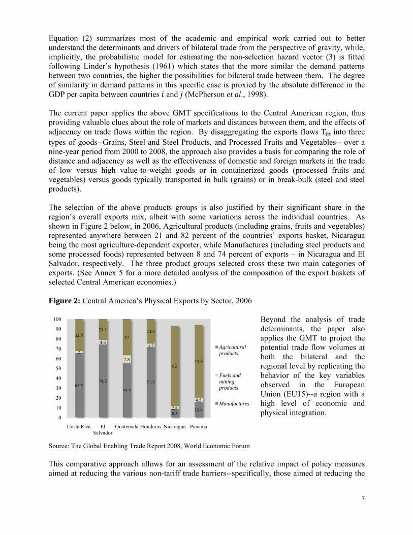
Equation (2) summarizes most of the academic and empirical work carried out to better understand the determinants and drivers of bilateral trade from the perspective of gravity, while, implicitly, the probabilistic model for estimating the non-selection hazard vector (3) is fitted following Linder’s hypothesis (1961) which states that the more similar the demand patterns between two countries, the higher the possibilities for bilateral trade between them. The degree of similarity in demand patterns in this specific case is proxied by the absolute difference in the GDP per capita between countries and (McPherson et al., 1998). The current paper applies the above GMT specifications to the Central American region, thus providing valuable clues about the role of markets and distances between them, and the effects of adjacency on trade flows within the region. By disaggregating the exports flows T into three types of goods--Grains, Steel and Steel Products, and Processed Fruits and Vegetables-- over a nine-year period from 2000 to 2008, the approach also provides a basis for comparing the role of distance and adjacency as well as the effectiveness of domestic and foreign markets in the trade of low versus high value-to-weight goods or in containerized goods (processed fruits and vegetables) versus goods typically transported in bulk (grains) or in break-bulk (steel and steel products). The selection of the above products groups is also justified by their significant share in the region’s overall exports mix, albeit with some variations across the individual countries. As shown in Figure 2 below, in 2006, Agricultural products (including grains, fruits and vegetables) represented anywhere between 21 and 82 percent of the countries’ exports basket, Nicaragua being the most agriculture-dependent exporter, while Manufactures (including steel products and some processed foods) represented between 8 and 74 percent of exports – in Nicaragua and El Salvador, respectively. The three product groups selected cross these two main categories of exports. (See Annex 5 for a more detailed analysis of the composition of the export baskets of selected Central American economies.) Figure 2: Central America’s Physical Exports by Sector, 2006

Beyond the analysis of trade determinants, the paper also applies the GMT to project the potential trade flow volumes at both the bilateral and the regional level by replicating the behavior of the key variables observed in the European Union (EU15)--a region with a high level of economic and physical integration.

Source: The Global Enabling Trade Report 2008, World Economic Forum This comparative approach allows for an assessment of the relative impact of policy measures aimed at reducing the various non-tariff trade barriers--specifically, those aimed at reducing the

65.574.2

55.2

71.7

8.515.6

2

4.6

7.8

3.7

2.8

4.5

32.521.1

3724.6

8273.9

0

10

20

30

40

50

60

70

80

90

100

Costa Rica El Salvador

Guatemala Honduras Nicaragua Panama

Agricultural products

Fuels and mining products

Manufactures

8

economic distance between two countries (geographic distance adjusted by time penalties caused by additional burdens posed by poor road conditions and congestion) and improving efficiency at border crossings. 2. Preliminary Results: Part 1 The first set of GMT estimations is organized as follows. The model is estimated using intraregional bilateral export flow data for the more integrated part of the European Union (EU15) and, second, for the Central America region. Estimations for both regions were first carried out in terms of total exports (measured in US$) and then for the disaggregated groups of goods: (i) Grains, including rice, maize, wheat, and barley, in both value (US$) and volume (kg) terms; (ii) Steel and Steel products, including ingots and other primary forms, iron and steel castings, tubes, rods, pipes and fittings, universals, iron and steel bars, rails and railway track construction materials, in both value and volume terms; and (iii) Processed Fruits & Vegetables in both value and volume terms. Estimations were carried out over a nine-year period from 2000 to 2008 controlling by country-pair fixed effects in a pooled regression. In the figures, results are presented at the 10-percent level of significance. 2.1. Establishing a Benchmark for Central America’s Spatial Integration

The results obtained for the EU15 countries for total intraregional exports (Figure 3) correspond to what is expected according to the intuition underlying the GMT theory: the GDP of both the importing and the exporting countries is significant and positively related to export flows, while the distance between each pair of economies has a significant and negative impact on trade, whereby an increase in distance by 1 percent reduces the expected exports by 0.93 percent. Similarly, as expected, adjacency represents opportunities for increasing exports within a highly-integrated region. Expressed as the percentage change in total exports,8 EU15 countries that share frontiers have 83 percent higher expected bilateral export flows than countries that do not.9 Positive and significant effects associated with adjacency, although of different magnitude, have also been found in studies focusing on other European economic blocks - 56 percent (World Bank, 2005), the Latin America and the Caribbean Region overall - 174 percent (Carrillo and Li, 2002), and in large country-samples covering the rest of the world - 289 percent (World Economic Forum, 2008).

8 The discrete change in expected exports correspond to ∆

|

|1

.

. 1 1 9 Expressed as ( 1).

9

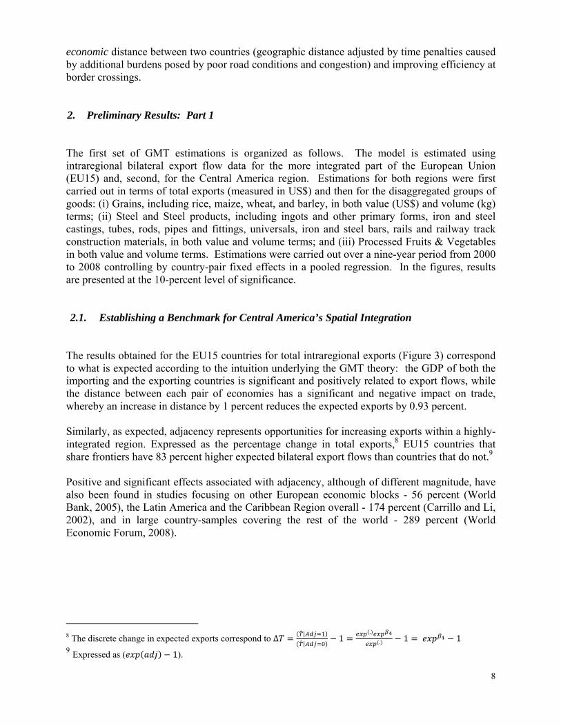
Figure 3: Model results for EU15 Intraregional Trade: Total Export Value

Once the model is disaggregated, the Importers’ GDP loses importance when compared to the Exporters’, especially in Grains and Processed Food. As shown in Figure 1 in Annex 1, on average, an increase in the GDP of the exporting country by 1 percent increases the expected exports from that country by about 1.4 percent (Grains), 1 percent (Steel) and 1.2 percent (Processed Fruits and Vegetables).

Source: World Bank LCSSD Economics Unit (2010) The distance effect, as expected, is negative and significant, with much larger negative impacts on the trade of the higher weight, lower value goods ( Grains and Steel) than in the containerized goods (Processed Food) or in the overall trade model. On average, an increase in distance by 1 percent reduces the total expected bilateral exports by 0.9 percent, while, in the case of the Steel exports, an increase in distance by 1 percent reduces the expected exports in value and volume terms by 1.2 and 1.4 percent, respectively. The “adjacency effect” on trade is significant all around although it is greater on the separate export flows of Grains, Steel, and Processed Foods than that observed in the overall trade model. In all three cases, "adjacency" increases the expected exports by over 300 percent,10 although, in the case of Steel exports expressed in volume terms, that effect is slightly lower (243 percent). The higher adjacency impact in the disaggregated sample vis-à-vis the overall trade sample could be explained by the comparatively greater role of overland transport modes in the transportation of bulk and break-bulk products (Grains, Steel) and containerized goods (Processed Foods), with other transport modes being more important in the export of most other types of goods, some of which (e.g. high-tech products) constitute a significant share in the overall basket of exports of individual EU countries and thus may drive the “adjacency” coefficients for the overall trade sample, particularly when measured in value terms.

2.2. Results for the CA Intraregional Trade Only

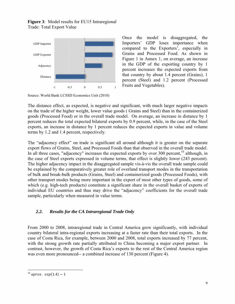
From 2000 to 2008, intraregional trade in Central America grew significantly, with individual country bilateral intra-regional exports increasing at a faster rate than their total exports. In the case of Costa Rica, for example, between 2000 and 2008, total exports increased by 77 percent, with the strong growth rate partially attributed to China becoming a major export partner. In contrast, however, the growth of Costa Rica’s exports to the rest of the Central America region was even more pronounced-- a combined increase of 130 percent (Figure 4).

10 . 1.4 1

-1 -0.5 0 0.5 1

Distance

Adjacency

GDP Exporter

GDP Importer

10

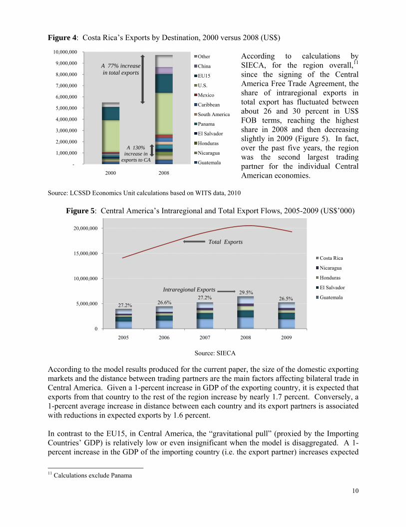
Figure 4: Costa Rica’s Exports by Destination, 2000 versus 2008 (US$) According to calculations by SIECA, for the region overall,11 since the signing of the Central America Free Trade Agreement, the share of intraregional exports in total export has fluctuated between about 26 and 30 percent in US$ FOB terms, reaching the highest share in 2008 and then decreasing slightly in 2009 (Figure 5). In fact, over the past five years, the region was the second largest trading partner for the individual Central American economies.

Source: LCSSD Economics Unit calculations based on WITS data, 2010

Figure 5: Central America’s Intraregional and Total Export Flows, 2005-2009 (US$’000)

Source: SIECA

According to the model results produced for the current paper, the size of the domestic exporting markets and the distance between trading partners are the main factors affecting bilateral trade in Central America. Given a 1-percent increase in GDP of the exporting country, it is expected that exports from that country to the rest of the region increase by nearly 1.7 percent. Conversely, a 1-percent average increase in distance between each country and its export partners is associated with reductions in expected exports by 1.6 percent. In contrast to the EU15, in Central America, the “gravitational pull” (proxied by the Importing Countries’ GDP) is relatively low or even insignificant when the model is disaggregated. A 1-percent increase in the GDP of the importing country (i.e. the export partner) increases expected

11 Calculations exclude Panama

0

5,000,000

10,000,000

15,000,000

20,000,000

2005 2006 2007 2008 2009

Costa Rica

Nicaragua

Honduras

El Salvador

Guatemala

Intraregional Exports

Total Exports

27.2% 26.6%27.2%

29.5%26.5%

-

1,000,000

2,000,000

3,000,000

4,000,000

5,000,000

6,000,000

7,000,000

8,000,000

9,000,000

10,000,000

2000 2008

Other

China

EU15

U.S.

Mexico

Caribbean

South America

Panama

El Salvador

Honduras

Nicaragua

Guatemala

A 77% increase in total exports

A 130% increase in

exports to CA

11

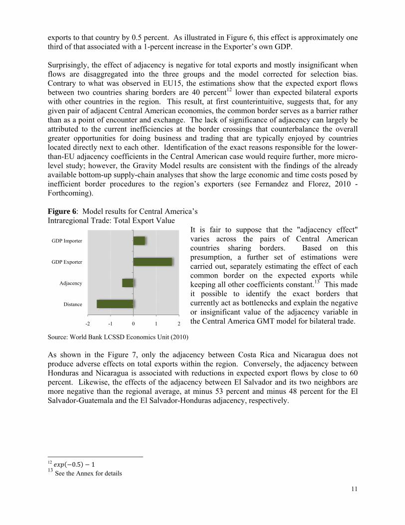
exports to that country by 0.5 percent. As illustrated in Figure 6, this effect is approximately one third of that associated with a 1-percent increase in the Exporter’s own GDP. Surprisingly, the effect of adjacency is negative for total exports and mostly insignificant when flows are disaggregated into the three groups and the model corrected for selection bias. Contrary to what was observed in EU15, the estimations show that the expected export flows between two countries sharing borders are 40 percent12 lower than expected bilateral exports with other countries in the region. This result, at first counterintuitive, suggests that, for any given pair of adjacent Central American economies, the common border serves as a barrier rather than as a point of encounter and exchange. The lack of significance of adjacency can largely be attributed to the current inefficiencies at the border crossings that counterbalance the overall greater opportunities for doing business and trading that are typically enjoyed by countries located directly next to each other. Identification of the exact reasons responsible for the lower-than-EU adjacency coefficients in the Central American case would require further, more micro-level study; however, the Gravity Model results are consistent with the findings of the already available bottom-up supply-chain analyses that show the large economic and time costs posed by inefficient border procedures to the region’s exporters (see Fernandez and Florez, 2010 - Forthcoming). Figure 6: Model results for Central America’s Intraregional Trade: Total Export Value

It is fair to suppose that the "adjacency effect" varies across the pairs of Central American countries sharing borders. Based on this presumption, a further set of estimations were carried out, separately estimating the effect of each common border on the expected exports while keeping all other coefficients constant.13 This made it possible to identify the exact borders that currently act as bottlenecks and explain the negative or insignificant value of the adjacency variable in the Central America GMT model for bilateral trade.

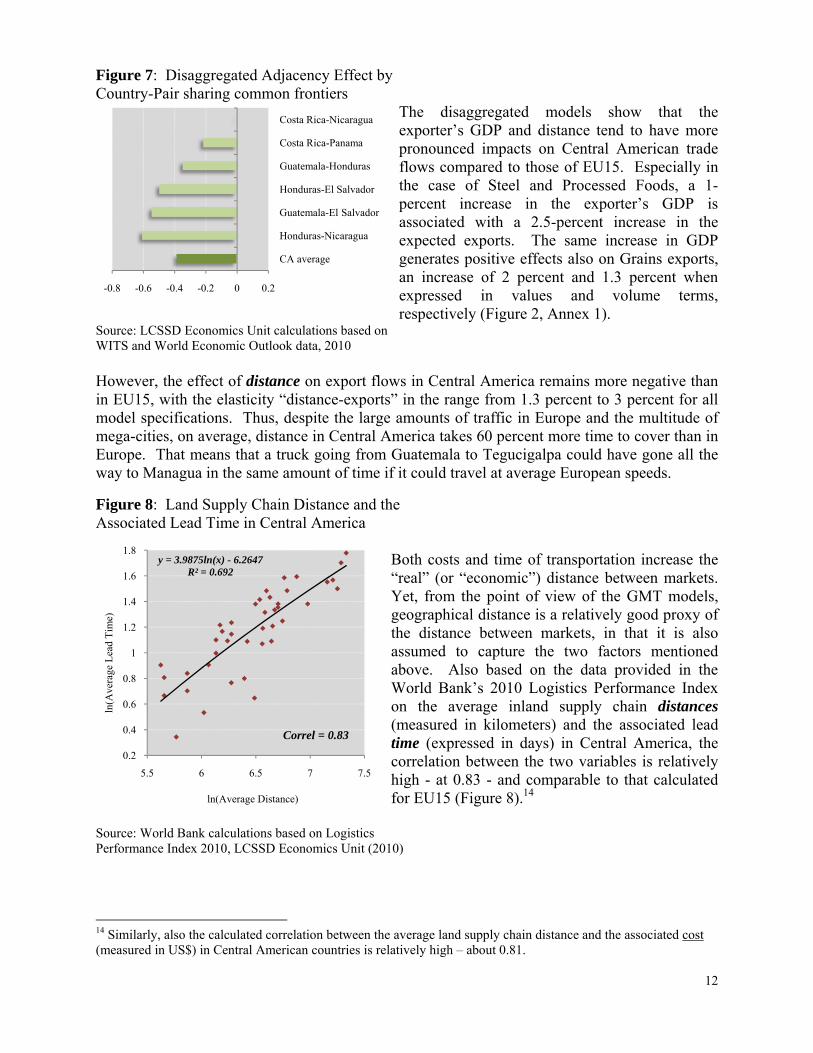
Source: World Bank LCSSD Economics Unit (2010) As shown in the Figure 7, only the adjacency between Costa Rica and Nicaragua does not produce adverse effects on total exports within the region. Conversely, the adjacency between Honduras and Nicaragua is associated with reductions in expected export flows by close to 60 percent. Likewise, the effects of the adjacency between El Salvador and its two neighbors are more negative than the regional average, at minus 53 percent and minus 48 percent for the El Salvador-Guatemala and the El Salvador-Honduras adjacency, respectively.

12 0.5 1 13 See the Annex for details

-2 -1 0 1 2

Distance

Adjacency

GDP Exporter

GDP Importer

12

y = 3.9875ln(x) - 6.2647R² = 0.692

0.2

0.4

0.6

0.8

1

1.2

1.4

1.6

1.8

5.5 6 6.5 7 7.5

ln(A

vera

ge L

ead

Tim

e)

ln(Average Distance)

Correl = 0.83

Figure 7: Disaggregated Adjacency Effect by Country-Pair sharing common frontiers

The disaggregated models show that the exporter’s GDP and distance tend to have more pronounced impacts on Central American trade flows compared to those of EU15. Especially in the case of Steel and Processed Foods, a 1-percent increase in the exporter’s GDP is associated with a 2.5-percent increase in the expected exports. The same increase in GDP generates positive effects also on Grains exports, an increase of 2 percent and 1.3 percent when expressed in values and volume terms, respectively (Figure 2, Annex 1).

Source: LCSSD Economics Unit calculations based on WITS and World Economic Outlook data, 2010 However, the effect of distance on export flows in Central America remains more negative than in EU15, with the elasticity “distance-exports” in the range from 1.3 percent to 3 percent for all model specifications. Thus, despite the large amounts of traffic in Europe and the multitude of mega-cities, on average, distance in Central America takes 60 percent more time to cover than in Europe. That means that a truck going from Guatemala to Tegucigalpa could have gone all the way to Managua in the same amount of time if it could travel at average European speeds.

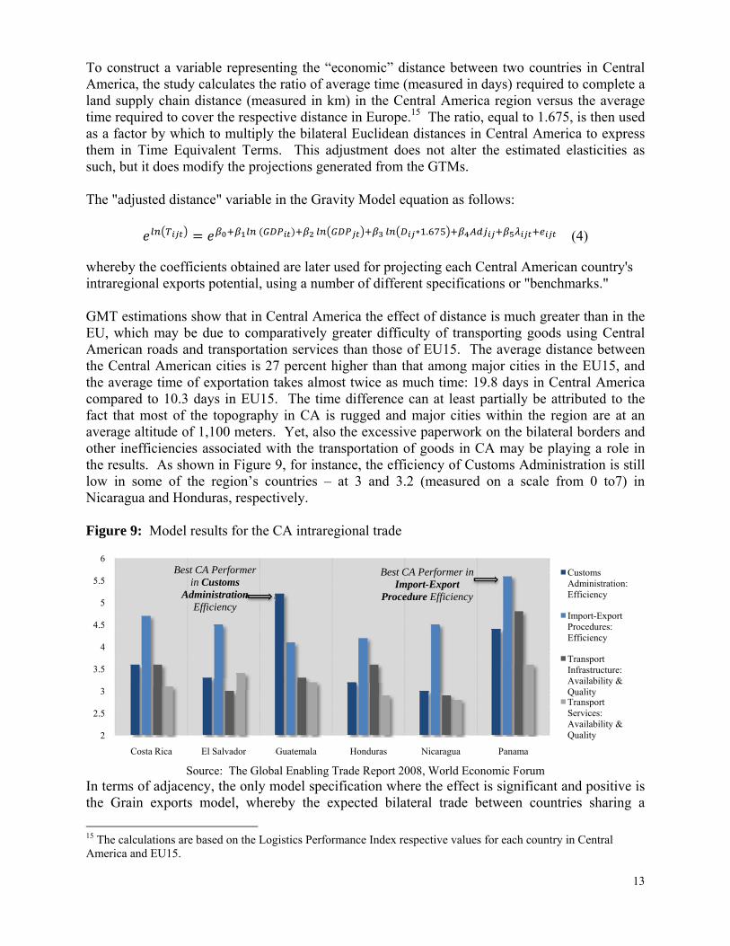
Figure 8: Land Supply Chain Distance and the Associated Lead Time in Central America

Both costs and time of transportation increase the “real” (or “economic”) distance between markets. Yet, from the point of view of the GMT models, geographical distance is a relatively good proxy of the distance between markets, in that it is also assumed to capture the two factors mentioned above. Also based on the data provided in the World Bank’s 2010 Logistics Performance Index on the average inland supply chain distances (measured in kilometers) and the associated lead time (expressed in days) in Central America, the correlation between the two variables is relatively high - at 0.83 - and comparable to that calculated for EU15 (Figure 8).14

Source: World Bank calculations based on Logistics Performance Index 2010, LCSSD Economics Unit (2010)

14 Similarly, also the calculated correlation between the average land supply chain distance and the associated cost (measured in US$) in Central American countries is relatively high – about 0.81.

-0.8 -0.6 -0.4 -0.2 0 0.2

CA average

Honduras-Nicaragua

Guatemala-El Salvador

Honduras-El Salvador

Guatemala-Honduras

Costa Rica-Panama

Costa Rica-Nicaragua

13

To construct a variable representing the “economic” distance between two countries in Central America, the study calculates the ratio of average time (measured in days) required to complete a land supply chain distance (measured in km) in the Central America region versus the average time required to cover the respective distance in Europe.15 The ratio, equal to 1.675, is then used as a factor by which to multiply the bilateral Euclidean distances in Central America to express them in Time Equivalent Terms. This adjustment does not alter the estimated elasticities as such, but it does modify the projections generated from the GTMs. The "adjusted distance" variable in the Gravity Model equation as follows:

. (4)

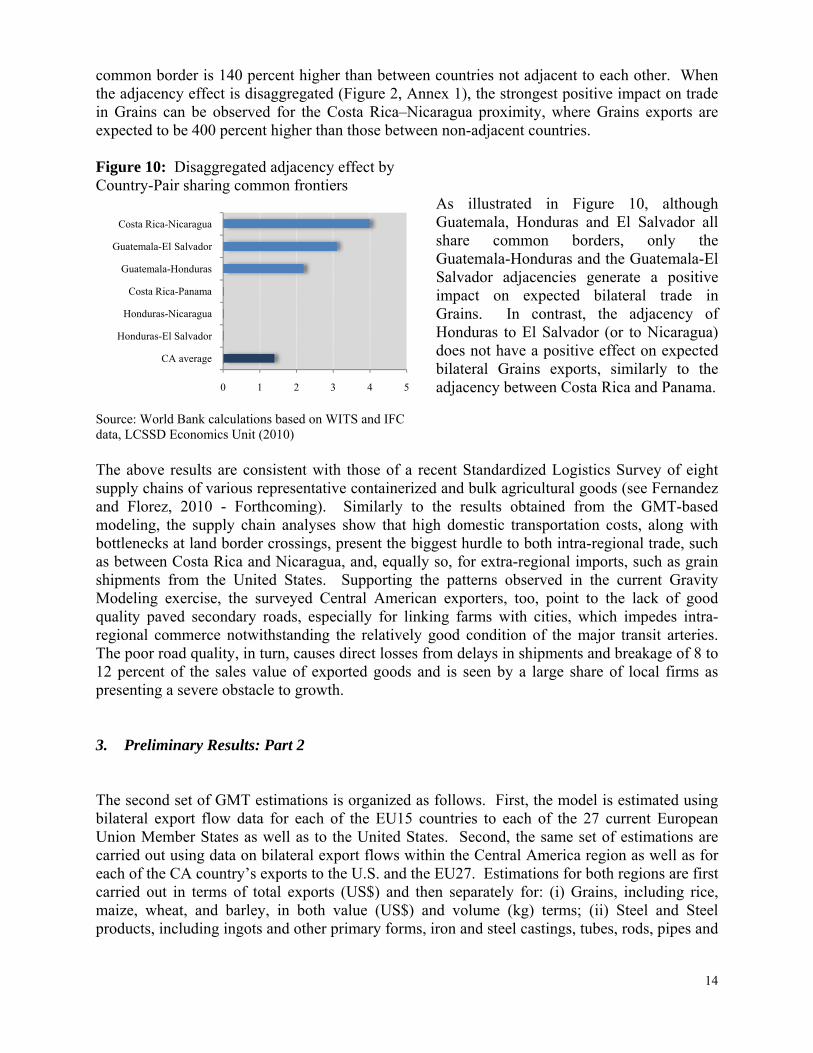
whereby the coefficients obtained are later used for projecting each Central American country's intraregional exports potential, using a number of different specifications or "benchmarks." GMT estimations show that in Central America the effect of distance is much greater than in the EU, which may be due to comparatively greater difficulty of transporting goods using Central American roads and transportation services than those of EU15. The average distance between the Central American cities is 27 percent higher than that among major cities in the EU15, and the average time of exportation takes almost twice as much time: 19.8 days in Central America compared to 10.3 days in EU15. The time difference can at least partially be attributed to the fact that most of the topography in CA is rugged and major cities within the region are at an average altitude of 1,100 meters. Yet, also the excessive paperwork on the bilateral borders and other inefficiencies associated with the transportation of goods in CA may be playing a role in the results. As shown in Figure 9, for instance, the efficiency of Customs Administration is still low in some of the region’s countries – at 3 and 3.2 (measured on a scale from 0 to7) in Nicaragua and Honduras, respectively. Figure 9: Model results for the CA intraregional trade

Source: The Global Enabling Trade Report 2008, World Economic Forum In terms of adjacency, the only model specification where the effect is significant and positive is the Grain exports model, whereby the expected bilateral trade between countries sharing a

15 The calculations are based on the Logistics Performance Index respective values for each country in Central America and EU15.

2

2.5

3

3.5

4

4.5

5

5.5

6

Costa Rica El Salvador Guatemala Honduras Nicaragua Panama

Customs Administration: Efficiency

Import-Export Procedures: Efficiency

Transport Infrastructure: Availability & QualityTransport Services: Availability & Quality

Best CA Performer in Customs

Administration Efficiency

Best CA Performer in Import-Export

Procedure Efficiency

14

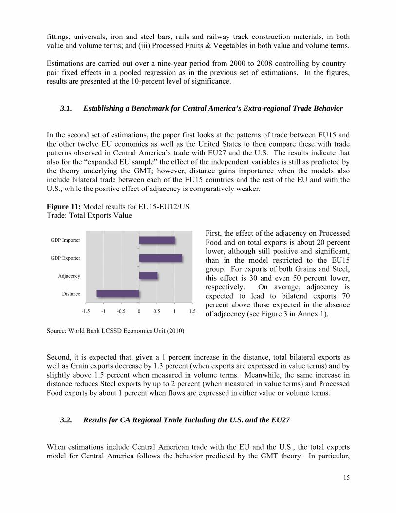
common border is 140 percent higher than between countries not adjacent to each other. When the adjacency effect is disaggregated (Figure 2, Annex 1), the strongest positive impact on trade in Grains can be observed for the Costa Rica–Nicaragua proximity, where Grains exports are expected to be 400 percent higher than those between non-adjacent countries. Figure 10: Disaggregated adjacency effect by Country-Pair sharing common frontiers

As illustrated in Figure 10, although Guatemala, Honduras and El Salvador all share common borders, only the Guatemala-Honduras and the Guatemala-El Salvador adjacencies generate a positive impact on expected bilateral trade in Grains. In contrast, the adjacency of Honduras to El Salvador (or to Nicaragua) does not have a positive effect on expected bilateral Grains exports, similarly to the adjacency between Costa Rica and Panama.

Source: World Bank calculations based on WITS and IFC data, LCSSD Economics Unit (2010) The above results are consistent with those of a recent Standardized Logistics Survey of eight supply chains of various representative containerized and bulk agricultural goods (see Fernandez and Florez, 2010 - Forthcoming). Similarly to the results obtained from the GMT-based modeling, the supply chain analyses show that high domestic transportation costs, along with bottlenecks at land border crossings, present the biggest hurdle to both intra-regional trade, such as between Costa Rica and Nicaragua, and, equally so, for extra-regional imports, such as grain shipments from the United States. Supporting the patterns observed in the current Gravity Modeling exercise, the surveyed Central American exporters, too, point to the lack of good quality paved secondary roads, especially for linking farms with cities, which impedes intra-regional commerce notwithstanding the relatively good condition of the major transit arteries. The poor road quality, in turn, causes direct losses from delays in shipments and breakage of 8 to 12 percent of the sales value of exported goods and is seen by a large share of local firms as presenting a severe obstacle to growth. 3. Preliminary Results: Part 2 The second set of GMT estimations is organized as follows. First, the model is estimated using bilateral export flow data for each of the EU15 countries to each of the 27 current European Union Member States as well as to the United States. Second, the same set of estimations are carried out using data on bilateral export flows within the Central America region as well as for each of the CA country’s exports to the U.S. and the EU27. Estimations for both regions are first carried out in terms of total exports (US$) and then separately for: (i) Grains, including rice, maize, wheat, and barley, in both value (US$) and volume (kg) terms; (ii) Steel and Steel products, including ingots and other primary forms, iron and steel castings, tubes, rods, pipes and

0 1 2 3 4 5

CA average

Honduras-El Salvador

Honduras-Nicaragua

Costa Rica-Panama

Guatemala-Honduras

Guatemala-El Salvador

Costa Rica-Nicaragua

15

fittings, universals, iron and steel bars, rails and railway track construction materials, in both value and volume terms; and (iii) Processed Fruits & Vegetables in both value and volume terms. Estimations are carried out over a nine-year period from 2000 to 2008 controlling by country–pair fixed effects in a pooled regression as in the previous set of estimations. In the figures, results are presented at the 10-percent level of significance.

3.1. Establishing a Benchmark for Central America’s Extra-regional Trade Behavior

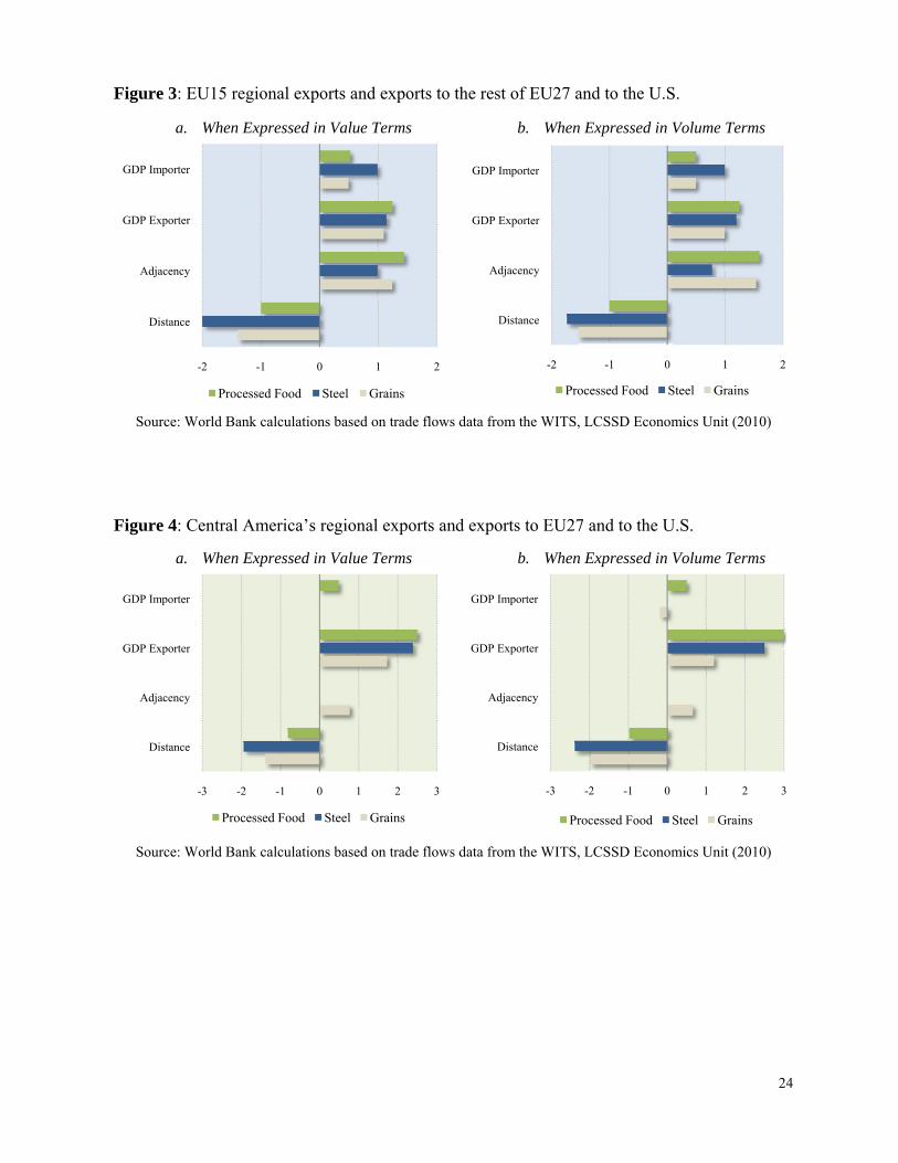
In the second set of estimations, the paper first looks at the patterns of trade between EU15 and the other twelve EU economies as well as the United States to then compare these with trade patterns observed in Central America’s trade with EU27 and the U.S. The results indicate that also for the “expanded EU sample” the effect of the independent variables is still as predicted by the theory underlying the GMT; however, distance gains importance when the models also include bilateral trade between each of the EU15 countries and the rest of the EU and with the U.S., while the positive effect of adjacency is comparatively weaker. Figure 11: Model results for EU15-EU12/US Trade: Total Exports Value

First, the effect of the adjacency on Processed Food and on total exports is about 20 percent lower, although still positive and significant, than in the model restricted to the EU15 group. For exports of both Grains and Steel, this effect is 30 and even 50 percent lower, respectively. On average, adjacency is expected to lead to bilateral exports 70 percent above those expected in the absence of adjacency (see Figure 3 in Annex 1).

Source: World Bank LCSSD Economics Unit (2010) Second, it is expected that, given a 1 percent increase in the distance, total bilateral exports as well as Grain exports decrease by 1.3 percent (when exports are expressed in value terms) and by slightly above 1.5 percent when measured in volume terms. Meanwhile, the same increase in distance reduces Steel exports by up to 2 percent (when measured in value terms) and Processed Food exports by about 1 percent when flows are expressed in either value or volume terms.

3.2. Results for CA Regional Trade Including the U.S. and the EU27 When estimations include Central American trade with the EU and the U.S., the total exports model for Central America follows the behavior predicted by the GMT theory. In particular,

-1.5 -1 -0.5 0 0.5 1 1.5

Distance

Adjacency

GDP Exporter

GDP Importer

16

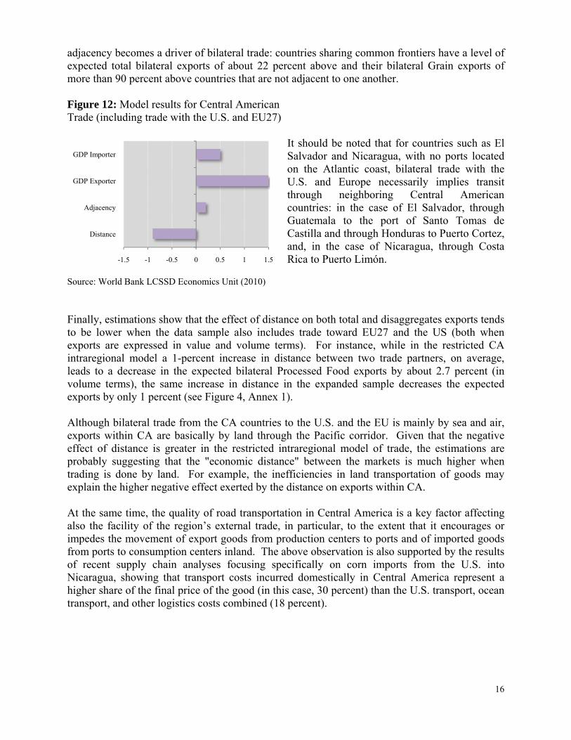
adjacency becomes a driver of bilateral trade: countries sharing common frontiers have a level of expected total bilateral exports of about 22 percent above and their bilateral Grain exports of more than 90 percent above countries that are not adjacent to one another. Figure 12: Model results for Central American Trade (including trade with the U.S. and EU27)

It should be noted that for countries such as El Salvador and Nicaragua, with no ports located on the Atlantic coast, bilateral trade with the U.S. and Europe necessarily implies transit through neighboring Central American countries: in the case of El Salvador, through Guatemala to the port of Santo Tomas de Castilla and through Honduras to Puerto Cortez, and, in the case of Nicaragua, through Costa Rica to Puerto Limón.

Source: World Bank LCSSD Economics Unit (2010) Finally, estimations show that the effect of distance on both total and disaggregates exports tends to be lower when the data sample also includes trade toward EU27 and the US (both when exports are expressed in value and volume terms). For instance, while in the restricted CA intraregional model a 1-percent increase in distance between two trade partners, on average, leads to a decrease in the expected bilateral Processed Food exports by about 2.7 percent (in volume terms), the same increase in distance in the expanded sample decreases the expected exports by only 1 percent (see Figure 4, Annex 1). Although bilateral trade from the CA countries to the U.S. and the EU is mainly by sea and air, exports within CA are basically by land through the Pacific corridor. Given that the negative effect of distance is greater in the restricted intraregional model of trade, the estimations are probably suggesting that the "economic distance" between the markets is much higher when trading is done by land. For example, the inefficiencies in land transportation of goods may explain the higher negative effect exerted by the distance on exports within CA. At the same time, the quality of road transportation in Central America is a key factor affecting also the facility of the region’s external trade, in particular, to the extent that it encourages or impedes the movement of export goods from production centers to ports and of imported goods from ports to consumption centers inland. The above observation is also supported by the results of recent supply chain analyses focusing specifically on corn imports from the U.S. into Nicaragua, showing that transport costs incurred domestically in Central America represent a higher share of the final price of the good (in this case, 30 percent) than the U.S. transport, ocean transport, and other logistics costs combined (18 percent).

-1.5 -1 -0.5 0 0.5 1 1.5

Distance

Adjacency

GDP Exporter

GDP Importer

17

4. Potential Intraregional Exports in Central America One of the main benefits of the GTM is that it allows projecting the "potential level" of exports based on a specific set of coefficients. In turn, the ratio between the observed and the potential export flows provides a measure of the closeness ─ or proximity index─ of a specific country or country-pair to its expected exports level ─ expectations frontier. Following Benedictis and Vicarelli (2005), this closeness measure can be expressed as:

(5)

Where captures the observed export flows from the exporter country to the importer country and are the expected exports flows generated by the gravity equation. To calculate the potential export flows, four different sets of coefficients were used for calculating , resulting in four different scenarios or “proximity indices.” The first scenario is based on the coefficients for the CA intra-regional trade model (Figure 6). The second one projects the exports flows in CA from the estimated coefficients obtained for the EU15 intra-regional model (Figure 3). A third scenario is obtained by applying the highest country-pair adjacency coefficient, obtained from the disaggregated GTM for Central America (with results illustrated in Figures 7 and 10),16 while the fourth scenario applies the adjacency coefficient resulting from the EU15 intra-regional model (Figure 3). Figure 13 below illustrates the results obtained from the four different scenarios, in this case, comparing Costa Rica with Honduras. In Costa Rica’s case, the observed-to-projected exports are close to the unconstrained Expectations Frontier (i.e. a ratio equivalent to 1), except for when the country’s currently observed exports are compared to what its exports would be expected to be under the assumption of an “EU15-like” behavior of all the independent trade variables (distance, adjacency, and the GDP of both the exporting and the importing country). In the case of Honduras, on the other hand, the ratio is far from 1 in all of the scenarios, including when the country’s observed exports are compared to what they would be expected to be assuming an adjacency effect equivalent to the adjacency effect of the best performer in Central America.

16 For Grains (in volume and value terms) and Overall Trade (in value terms) the best country-pair adjacency effect corresponds to the Costa Rica- Nicaragua; for Steel and Processed Fruit & Vegetable exports, even the best “Adjacency Performance” across the country couples is 0.

18

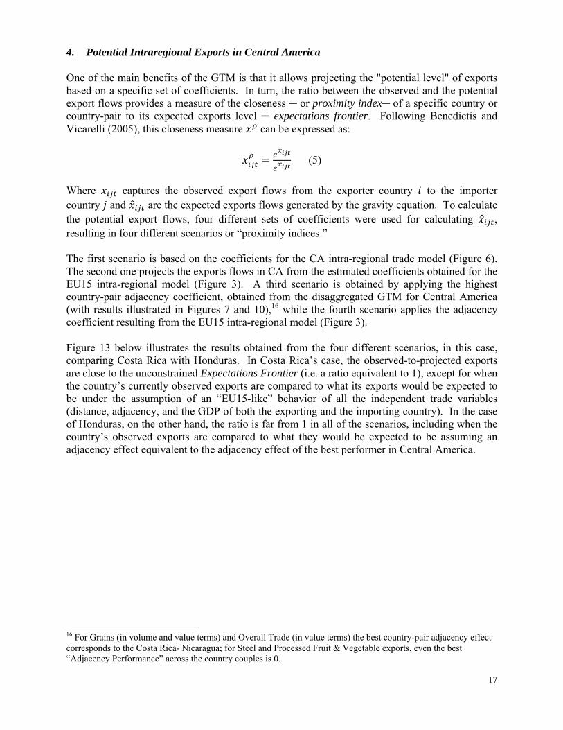
Figure 13: Closeness of CA’s total intra-regional exports value to the Unconstrained Expectations Frontier

Source: World Bank calculations based on trade flows data from WITS, LCSSD Economics Unit (2010)

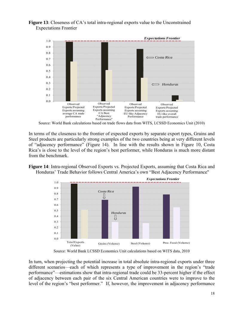
In terms of the closeness to the frontier of expected exports by separate export types, Grains and Steel products are particularly strong examples of the two countries being at very different levels of “adjacency performance” (Figure 14). In line with the results shown in Figure 10, Costa Rica’s is close to the level of the region’s best performer, while Honduras is much more distant from the benchmark. Figure 14: Intra-regional Observed Exports vs. Projected Exports, assuming that Costa Rica and

Honduras’ Trade Behavior follows Central America’s own “Best Adjacency Performance"

Source: World Bank LCSSD Economics Unit calculations based on WITS data, 2010

In turn, when projecting the potential increase in total absolute intra-regional exports under three different scenarios—each of which represents a type of improvement in the region’s “trade performance”—estimations show that intra-regional trade could be 33-percent higher if the effect of adjacency between each pair of the six Central American countries were to improve to the level of the region’s “best performer.” If, however, the improvement in adjacency performance

0.0

0.1

0.2

0.3

0.4

0.5

0.6

0.7

0.8

0.9

1.0

OBS

ERVE

D/CA

_BASED

OBS

ERVE

D/CA

BP

AD_

BASED

OBS

ERVE

D/AD_

BASED

OBS

ERVE

D/EU

_BASED

Expectations Frontier

ObservedExports/Projected Exports assuming average CA trade

performance

ObservedExports/Projected Exports assuming

CA Best "Adjacency

Performance"

ObservedExports/Projected Exports assuming

EU-like Adjacency Performance

ObservedExports/Projected Exports assuming EU-like overall

trade performance

Costa Rica

Honduras

0.0

0.1

0.2

0.3

0.4

0.5

0.6

0.7

0.8

0.9

1.0

Total Exports (Value)

Grains (Volume) Steel (Volume) Proc. Food (Volume)

Costa Rica

Honduras

Expectations Frontier

19

was to the level of EU15, the potential increase would be as much as 55 percent.17 On the other hand, intra-regional exports would double if Central America were to become fully “spatially integrated” - i.e., if all of its key infrastructure integration and efficiency indicators were to improve to the level of EU15.18

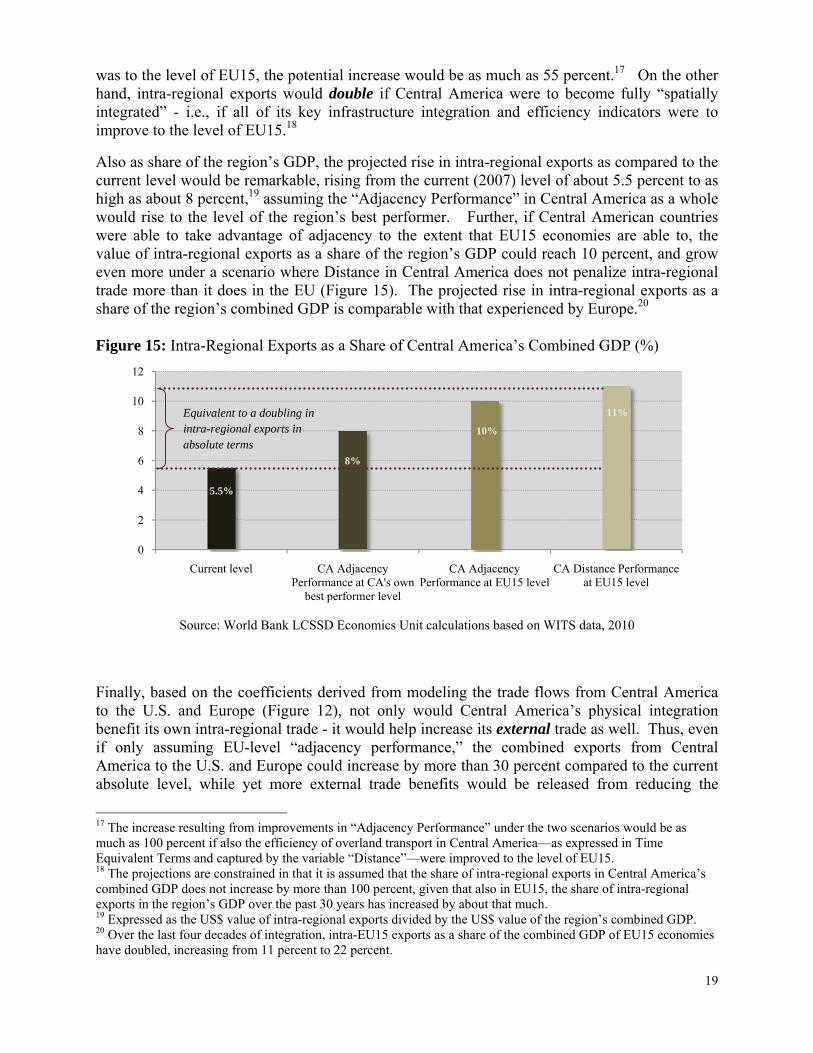
Also as share of the region’s GDP, the projected rise in intra-regional exports as compared to the current level would be remarkable, rising from the current (2007) level of about 5.5 percent to as high as about 8 percent,19 assuming the “Adjacency Performance” in Central America as a whole would rise to the level of the region’s best performer. Further, if Central American countries were able to take advantage of adjacency to the extent that EU15 economies are able to, the value of intra-regional exports as a share of the region’s GDP could reach 10 percent, and grow even more under a scenario where Distance in Central America does not penalize intra-regional trade more than it does in the EU (Figure 15). The projected rise in intra-regional exports as a share of the region’s combined GDP is comparable with that experienced by Europe.20 Figure 15: Intra-Regional Exports as a Share of Central America’s Combined GDP (%)

Source: World Bank LCSSD Economics Unit calculations based on WITS data, 2010

Finally, based on the coefficients derived from modeling the trade flows from Central America to the U.S. and Europe (Figure 12), not only would Central America’s physical integration benefit its own intra-regional trade - it would help increase its external trade as well. Thus, even if only assuming EU-level “adjacency performance,” the combined exports from Central America to the U.S. and Europe could increase by more than 30 percent compared to the current absolute level, while yet more external trade benefits would be released from reducing the

17 The increase resulting from improvements in “Adjacency Performance” under the two scenarios would be as much as 100 percent if also the efficiency of overland transport in Central America—as expressed in Time Equivalent Terms and captured by the variable “Distance”—were improved to the level of EU15. 18 The projections are constrained in that it is assumed that the share of intra-regional exports in Central America’s combined GDP does not increase by more than 100 percent, given that also in EU15, the share of intra-regional exports in the region’s GDP over the past 30 years has increased by about that much. 19 Expressed as the US$ value of intra-regional exports divided by the US$ value of the region’s combined GDP. 20 Over the last four decades of integration, intra-EU15 exports as a share of the combined GDP of EU15 economies have doubled, increasing from 11 percent to 22 percent.

0

2

4

6

8

10

12

Current level CA Adjacency Performance at CA's own

best performer level

CA Adjacency Performance at EU15 level

CA Distance Performance at EU15 level

5.5%

8%

10%

11%Equivalent to a doubling in intra-regional exports in absolute terms

20

economic penalty imposed by the need to use sub-optimal roads and trucking services in covering overland road distances and from reducing the obstacles to greater “gravitational pull” from import markets.

5. Conclusions and Policy Implications

As highlighted by the Gravity Model–based results analyzed above, intra-regional trade in Central America does not behave like it does in a highly spatially-integrated region. Instead, it is still inhibited by a number of inefficiencies that overshadow the formal trade tariff and non–tariff barriers that have historically figured high on the regional integration agenda.

The economic distance between the markets of Central America is being distorted and magnified by a number of inefficiencies, including the poor road quality, the congestion at the border crossings and metropolitan areas, the inadequate supply of trucking services, and other overland transport inefficiencies. These factors may explain why in Central America the negative effect of distance on trade flows tends to be higher than in a spatially-integrated region.

Similarly, the results show that Central American economies fail to take advantage of adjacency - not only to the extent that it affects intra-regional trade patterns but also the region’s trade with the U.S. and other external partners. As highlighted by recent supply chain analyses that are able to capture these specific micro-level challenges, the reasons why country adjacency in Central America does not seem to exhibit the positive impact on trade flows that it would be expected to include burdensome customs procedures, delays, and lack of regulatory harmonization (e.g. in terms of phytosanitary standards for agricultural exports).

Finally, the Gravity Model results indicate that Central American countries are experiencing a lower “gravitational pull” from the nearby economies. Intuitively, this is due to poorly established trade linkages, an atomized shipping industry, little information sharing on cargo and backhaul, and relatively few options and competition for shipping (i.e. absence of coastal shipping, rail services, and low road density).

The overall policy implications of the above estimations are similar to those identified in the recent supply chain analyses carried out in Central America that, instead, highlight the micro-level challenges related to overland transport inefficiencies, burdensome border crossing procedures, and lack of regulatory harmonization posed. As highlighted previously, in order to reduce the inefficiencies that currently offset the positive benefits that Central American countries could obtain from being adjacent to one another, policy and regulatory actions need to be focused on improving the region’s border crossings, while additional investments and institutional coordination initiatives are warranted to reduce the ‘economic’— i.e. the cost- and time-equivalent—overland distance between production and consumption centers within the region.

21

References ADB (2009): Infrastructure for a Seamless Asia. Asian Development Bank.

Anderson, J. E. (2001): Gravity with Gravitas: a Solution to the Border Puzzle. Working Paper 8079, National Bureau of Economic Research, Cambridge, MA, January.

______ (1979): “A Theoretical Foundation for the Gravity Equation,” The American Economic Review, Vol. 69, No. 1, March, pp. 106-116.

Asia-Pacific Economic Cooperation Secretariat (2010): The Economic Impact of Enhanced Multimodal Connectivity in the APEC Region. APEC Policy Support Unit, June.

Bablu, S. and S. K. Mazumder (2006): “The Constrained Gravity Model with Power Function as a Cost Function,” Journal of Applied Mathematics and Decision Sciences, Volume 2006, Article ID 48632, pp. 1-13.

Balistreri, E. J. and R. H. Hillberry (2006): “Trade Fractions and Welfare in the Gravity Model: How Much of the Iceberg Melts?” The Canadian Journal of Economics / Revue Canadienne d’Economique, Vol. 39, No. 1, February, pp. 247-265.

Balogun, E. D. (2008): An Empirical Test of Trade Gravity Model Criteria for the West African Monetary Zone (WAMZ). University of Lagos, Lagos, Nigeria, February 9.

Benedictis, L. de and C. Vicarelli (2005): “Trade Potentials in Gravity Panel Data Models,” Topics in Economic Analysis & Policy, Vol. 5, Issue 1, Article 20.

Deardoff, A. V. (1995): Determinants of Bilateral Trade: Does Gravity Work in a Neoclassical World? Working Paper 5377, NBER Working Paper Series, National Bureau of Economic Research, December.

Dowrick, S. and J. Golley (2004): “Trade Openness and Growth: Who Benefits?” in Oxford Review of Economic Policy, Vol. 20, Issue 1, pp. 38-56, Oxford University Press.

Fernández, R. and S. Flórez (2010 - Forthcoming): “Supply Chain Analyses of Exports and Imports of Agricultural Products: Case Studies of Costa Rica, Honduras, and Nicaragua” in Policy Research Working Paper Series. Washington. D.C.: The World Bank.

Fidrmuc, J. (2008): Gravity Models in Integrated Panels. Springer-Verlag, September 23.

Helpman, E. (1987): “Imperfect Competition and International Trade: Evidence from Fourteen Industrial Countries,” Journal of the Japanese and International Economies 1, June, pp. 62-81.

Helpman, E., M. Melitz and Y. Rubinstein (2005): Trading Partners and Trading Volumes. March 31.

Hesse, H (2009): “Export Diversification and Economic Growth" in Richard S. Newfarmer, William Shaw & Peter Walkenhorst (editors), Breaking into New Markets: Emerging Lessons for Export Diversification, pp. 55-80. Washington, DC: The World Bank.

McCallum, J. (1995): “National Borders Matter: Canada-U.S. Regional Trade Patterns,” The American Economic Review, Vol. 85, No. 3, pp.615-623.

McPherson, M. A., M. R. Redfearn and M. A. Tieslau (1998): A Re-Examination of the Linder Hypothesis: a Random-Effects Tobit Approach. University of North Texas.

22

Samuelson, P. (1954): “The Transfer Problem and Transport Costs, II: Analysis of Effects of Trade Impediments,” The Economic Journal, Vol. 64, No. 254, June, pp. 264-289.

Schwartz, J., J. L. Guasch, G. Wilmsmeir, and A. Stokenberga (2009): “Logistics, Transport and Food Prices in LAC: Policy Guidance for Improving Efficiency and Reducing Costs,” Sustainable Development Occasional Paper Series, No. 2, August 2009, World Bank.

SIECA (2001): Estudio Centroamericano de Transporte. Informe de Síntesis, Plan Maestro de Transporte 2001-2010, February.

Wimsmeier, G. and J. Hoffmann (2008): “Liner Shipping Connectivity and Port Infrastructure as Determinants of Freight Rates in the Caribbean,” Maritime Economics & Logistics, 2008, 10, pp130–151.

World Bank (2004a): Guatemala Investment Climate Assessment.

_____ (2006a): El Salvador: Desarollos Económicos Recientes en Infraestructura.

_____ (2006b): Costa Rica Country Economic Memorandum.

_____ (2009): Uruguay Trade and Logistics: An Opportunity.

World Economic Forum (2008): Global Enabling Trade Report.

23

Annexes

Annex 1: Detailed Representation of Results

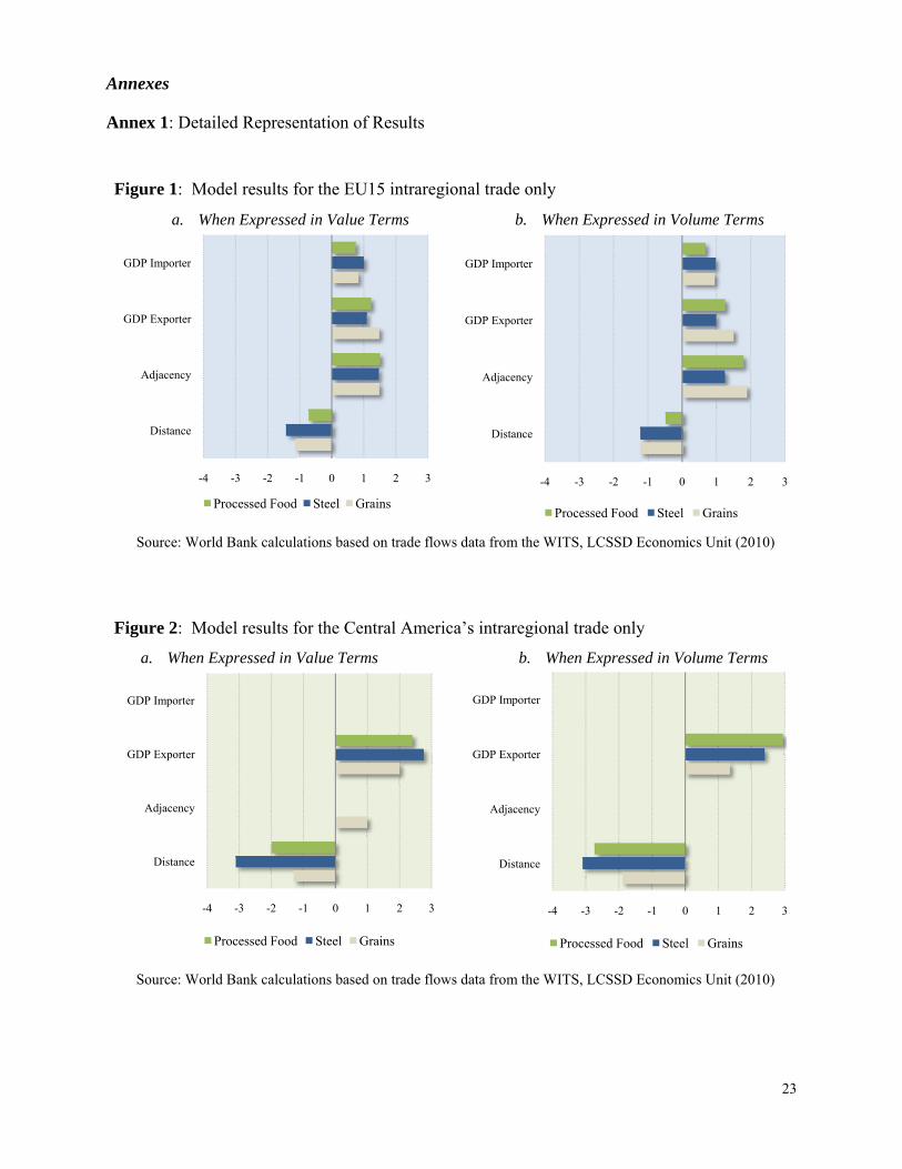
Figure 1: Model results for the EU15 intraregional trade only

a. When Expressed in Value Terms b. When Expressed in Volume Terms

Source: World Bank calculations based on trade flows data from the WITS, LCSSD Economics Unit (2010)

-4 -3 -2 -1 0 1 2 3

Distance

Adjacency

GDP Exporter

GDP Importer

Processed Food Steel Grains

-4 -3 -2 -1 0 1 2 3

Distance

Adjacency

GDP Exporter

GDP Importer


Figure 2: Model results for the Central America’s intraregional trade only



-4 -3 -2 -1 0 1 2 3

Distance

Adjacency

GDP Exporter

GDP Importer


-4 -3 -2 -1 0 1 2 3

Distance

Adjacency

GDP Exporter

GDP Importer


24

Figure 3: EU15 regional exports and exports to the rest of EU27 and to the U.S.



Figure 4: Central America’s regional exports and exports to EU27 and to the U.S.



-2 -1 0 1 2

Distance

Adjacency

GDP Exporter

GDP Importer


-2 -1 0 1 2

Distance

Adjacency

GDP Exporter

GDP Importer


-3 -2 -1 0 1 2 3

Distance

Adjacency

GDP Exporter

GDP Importer


-3 -2 -1 0 1 2 3

Distance

Adjacency

GDP Exporter

GDP Importer


25

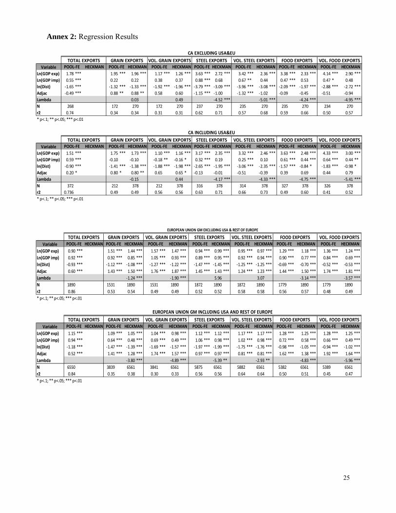
Annex 2: Regression Results

Variable

Ln(GDP exp) 1.78 *** 1.95 *** 1.96 *** 1.17 *** 1.26 *** 3.63 *** 2.72 *** 3.42 *** 2.36 *** 3.38 *** 2.33 *** 4.14 *** 2.90 ***

Ln(GDP imp) 0.55 *** 0.22 0.22 0.38 0.37 0.88 *** 0.68 0.67 ** 0.44 0.47 *** 0.53 0.47 * 0.48

ln(Dist) ‐1.65 *** ‐1.32 *** ‐1.33 *** ‐1.92 *** ‐1.96 *** ‐3.79 *** ‐3.09 *** ‐3.96 *** ‐3.08 *** ‐2.09 *** ‐1.97 *** ‐2.88 *** ‐2.72 ***

Adjac ‐0.49 *** 0.88 ** 0.88 ** 0.58 0.60 ‐1.15 *** ‐1.00 ‐1.32 *** ‐1.02 ‐0.09 ‐0.45 ‐0.51 ‐0.94

Lambda 0.03 0.49 ‐4.52 *** ‐5.01 *** ‐4.24 *** ‐4.95 ***

N 268 172 270 172 270 237 270 235 270 235 270 234 270

r2 0.74 0.34 0.34 0.31 0.31 0.62 0.71 0.57 0.68 0.59 0.66 0.50 0.57

* p<.1; ** p<.05; *** p<.01

Variable

Ln(GDP exp) 1.51 *** 1.75 *** 1.73 *** 1.10 *** 1.16 *** 3.17 *** 2.35 *** 3.32 *** 2.46 *** 3.63 *** 2.48 *** 4.33 *** 3.00 ***

Ln(GDP imp) 0.59 *** ‐0.10 ‐0.10 ‐0.18 ** ‐0.16 * 0.32 *** 0.19 0.25 *** 0.10 0.61 *** 0.44 *** 0.64 *** 0.44 **

ln(Dist) ‐0.90 *** ‐1.41 *** ‐1.38 *** ‐1.88 *** ‐1.98 *** ‐2.65 *** ‐1.95 *** ‐3.06 *** ‐2.35 *** ‐1.57 *** ‐0.84 * ‐1.83 *** ‐0.98 *

Adjac 0.20 * 0.80 * 0.80 ** 0.65 0.65 * ‐0.13 ‐0.01 ‐0.51 ‐0.39 0.39 0.69 0.44 0.79

Lambda ‐0.15 0.44 ‐4.17 *** ‐4.33 *** ‐4.75 *** ‐5.41 ***

N 372 212 378 212 378 316 378 314 378 327 378 326 378

r2 0.736 0.49 0.49 0.56 0.56 0.63 0.71 0.66 0.73 0.49 0.60 0.41 0.52

* p<.1; ** p<.05; *** p<.01

VOL. FOOD EXPORTSPOOL‐FE HECKMAN POOL‐FE HECKMAN

CA INCLUDING USA&EU

POOL‐FE HECKMAN POOL‐FE HECKMAN POOL‐FE HECKMAN POOL‐FE HECKMAN POOL‐FE HECKMAN

FOOD EXPORTSTOTAL EXPORTS GRAIN EXPORTS VOL. GRAIN EXPORTS STEEL EXPORTS VOL. STEEL EXPORTS

HECKMAN POOL‐FE HECKMAN POOL‐FE HECKMAN POOL‐FE HECKMAN POOL‐FE HECKMANPOOL‐FE HECKMAN POOL‐FE HECKMAN POOL‐FE

VOL. STEEL EXPORTS

CA EXCLUDING USA&EU

FOOD EXPORTS VOL. FOOD EXPORTSTOTAL EXPORTS GRAIN EXPORTS VOL. GRAIN EXPORTS STEEL EXPORTS

Variable

Ln(GDP exp) 0.90 *** 1.51 *** 1.44 *** 1.57 *** 1.47 *** 0.94 *** 0.99 *** 0.95 *** 0.97 *** 1.29 *** 1.18 *** 1.36 *** 1.24 ***

Ln(GDP imp) 0.92 *** 0.92 *** 0.85 *** 1.05 *** 0.93 *** 0.89 *** 0.95 *** 0.92 *** 0.94 *** 0.90 *** 0.77 *** 0.84 *** 0.69 ***

ln(Dist) ‐0.93 *** ‐1.12 *** ‐1.08 *** ‐1.27 *** ‐1.22 *** ‐1.47 *** ‐1.45 *** ‐1.25 *** ‐1.25 *** ‐0.69 *** ‐0.70 *** ‐0.52 *** ‐0.53 ***

Adjac 0.60 *** 1.43 *** 1.50 *** 1.76 *** 1.87 *** 1.45 *** 1.43 *** 1.24 *** 1.23 *** 1.44 *** 1.50 *** 1.74 *** 1.81 ***

Lambda ‐1.24 *** ‐1.90 *** 5.96 3.07 ‐3.14 *** ‐3.57 ***

N 1890 1531 1890 1531 1890 1872 1890 1872 1890 1779 1890 1779 1890

r2 0.86 0.53 0.54 0.49 0.49 0.52 0.52 0.58 0.58 0.56 0.57 0.48 0.49

* p<.1; ** p<.05; *** p<.01

Variable

Ln(GDP exp) 1.15 *** 1.09 *** 1.05 *** 1.04 *** 0.98 *** 1.12 *** 1.12 *** 1.17 *** 1.17 *** 1.28 *** 1.25 *** 1.28 *** 1.25 ***

Ln(GDP imp) 0.94 *** 0.64 *** 0.48 *** 0.69 *** 0.49 *** 1.06 *** 0.98 *** 1.02 *** 0.98 *** 0.72 *** 0.58 *** 0.66 *** 0.49 ***

ln(Dist) ‐1.18 *** ‐1.47 *** ‐1.39 *** ‐1.69 *** ‐1.57 *** ‐1.97 *** ‐1.99 *** ‐1.75 *** ‐1.76 *** ‐0.98 *** ‐1.05 *** ‐0.94 *** ‐1.02 ***

Adjac 0.52 *** 1.41 *** 1.28 *** 1.74 *** 1.57 *** 0.97 *** 0.97 *** 0.81 *** 0.81 *** 1.62 *** 1.38 *** 1.92 *** 1.64 ***

Lambda ‐3.80 *** ‐4.89 *** ‐5.39 ** ‐2.93 ** ‐4.83 *** ‐5.96 ***

N 6550 3839 6561 3841 6561 5875 6561 5882 6561 5382 6561 5389 6561

r2 0.84 0.35 0.38 0.30 0.33 0.56 0.56 0.64 0.64 0.50 0.51 0.45 0.47

* p<.1; ** p<.05; *** p<.01

POOL‐FE HECKMAN

EUROPEAN UNION GM INCLUDING USA AND REST OF EUROPE

VOL. STEEL EXPORTSTOTAL EXPORTS GRAIN EXPORTS VOL. FOOD EXPORTS

POOL‐FE HECKMANPOOL‐FEHECKMAN POOL‐FE HECKMAN POOL‐FE HECKMAN

FOOD EXPORTSPOOL‐FE HECKMANPOOL‐FE HECKMANPOOL‐FE HECKMAN POOL‐FE HECKMAN POOL‐FE HECKMAN POOL‐FE HECKMAN

VOL. GRAIN EXPORTS STEEL EXPORTSPOOL‐FE HECKMAN

HECKMANPOOL‐FE HECKMAN POOL‐FE

GRAIN EXPORTS VOL. GRAIN EXPORTS

EUROPEAN UNION GM EXCLUDING USA & REST OF EUROPE

VOL. STEEL EXPORTS FOOD EXPORTSSTEEL EXPORTS VOL. FOOD EXPORTSTOTAL EXPORTS

26

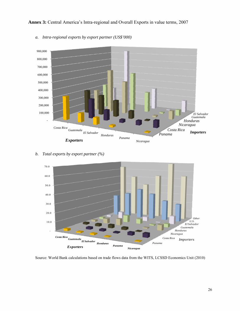
Annex 3: Central America’s Intra-regional and Overall Exports in value terms, 2007

a. Intra-regional exports by export partner (US$’000)

b. Total exports by export partner (%)


-

100,000

200,000

300,000

400,000

500,000

600,000

700,000

800,000

900,000

Costa RicaGuatemala

El SalvadorHonduras

PanamaNicaragua

PanamaCosta Rica

NicaraguaHonduras

GuatemalaEl Salvador

Exporters

Importers

-

10.0

20.0

30.0

40.0

50.0

60.0

70.0

Costa RicaGuatemala

El SalvadorHonduras

PanamaNicaragua

Panama

Costa Rica

NicaraguaHonduras

GuatemalaEl Salvador

U.S.Other

Exporters

Importers

27

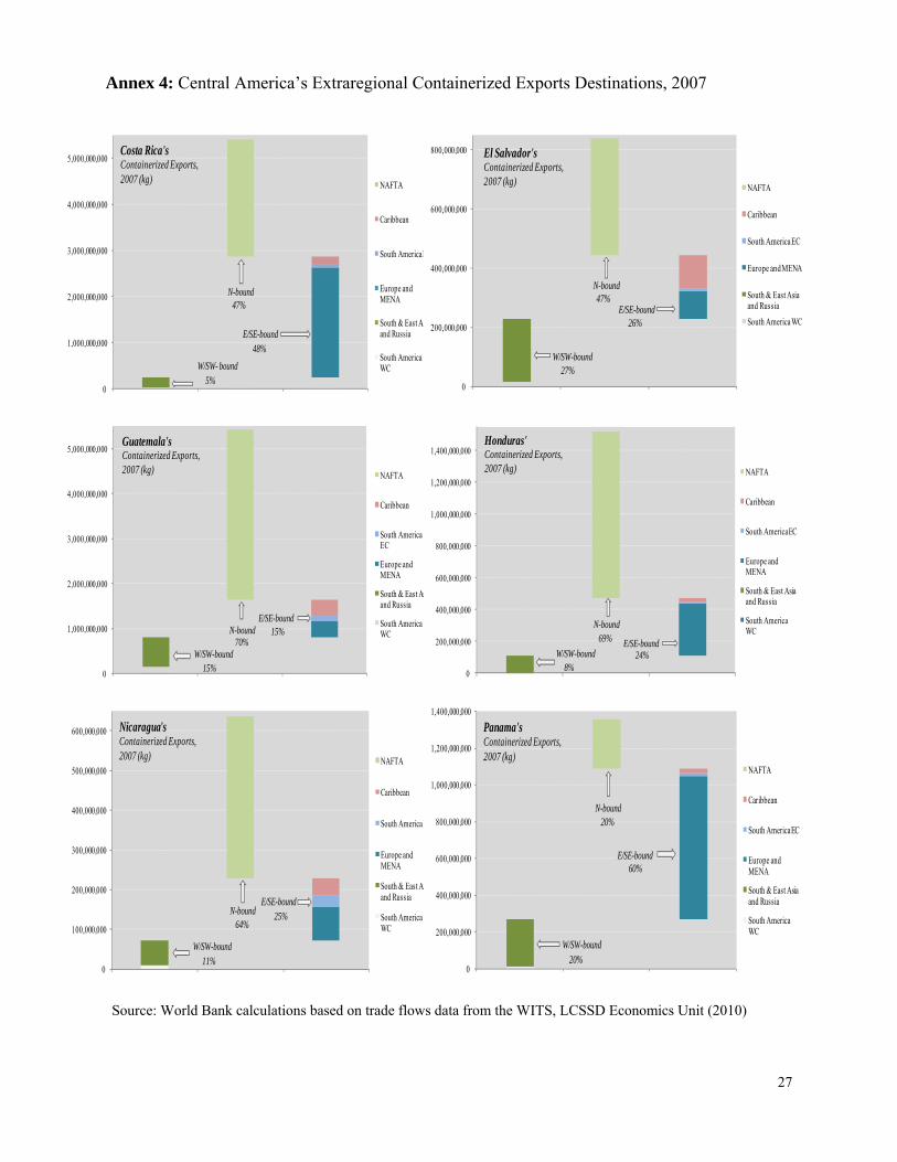
Annex 4: Central America’s Extraregional Containerized Exports Destinations, 2007


0

1,000,000,000

2,000,000,000

3,000,000,000

4,000,000,000

5,000,000,000

1 2 3

NAFTA

Caribbean

South America E

Europe and MENA

South & East Asand Russia

South America WCW/SW- bound

E/SE-bound

N-bound

Costa Rica's Containerized Exports,2007 (kg)

5%

48%

47%

0

200,000,000

400,000,000

600,000,000

800,000,000

1 2 3

NAFTA

Caribbean

South America EC

Europe and MENA

South & East Asia and Russia

South America WC

El Salvador's Containerized Exports,2007 (kg)

N-bound

W/SW-bound

E/SE-bound

27%

47%

26%

0

1,000,000,000

2,000,000,000

3,000,000,000

4,000,000,000

5,000,000,000

1 2 3

NAFTA

Caribbean

South America EC

Europe and MENA

South & East Asand Russia

South America WC

Guatemala'sContainerized Exports,2007 (kg)

N-bound

W/SW-bound

E/SE-bound15%

70%

15% 0

200,000,000

400,000,000

600,000,000

800,000,000

1,000,000,000

1,200,000,000

1,400,000,000

1 2 3

NAFTA

Caribbean

South America EC

Europe and MENA


South America WC

Honduras'Containerized Exports,2007 (kg)

N-bound

W/SW-boundE/SE-bound69%

8%24%

0

100,000,000

200,000,000

300,000,000

400,000,000

500,000,000

600,000,000

1 2 3

NAFTA

Caribbean

South America E

Europe and MENA

South & East Aand Russia

South America WC

Nicaragua'sContainerized Exports,2007 (kg)

N-bound

W/SW-bound

E/SE-bound25%

64%

11%0

200,000,000

400,000,000

600,000,000

800,000,000

1,000,000,000

1,200,000,000

1,400,000,000

1 2 3

NAFTA

Caribbean

South America EC

Europe and MENA


South America WC

Panama'sContainerized Exports,2007 (kg)

N-bound

W/SW-bound

E/SE-bound

20%

20%

60%

28

Annex 5: Export Structures of Selected Central American Economies21

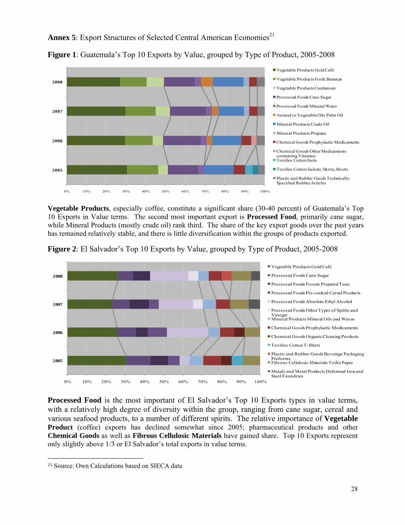
Figure 1: Guatemala’s Top 10 Exports by Value, grouped by Type of Product, 2005-2008

Vegetable Products, especially coffee, constitute a significant share (30-40 percent) of Guatemala’s Top 10 Exports in Value terms. The second most important export is Processed Food, primarily cane sugar, while Mineral Products (mostly crude oil) rank third. The share of the key export goods over the past years has remained relatively stable, and there is little diversification within the groups of products exported.

Figure 2: El Salvador’s Top 10 Exports by Value, grouped by Type of Product, 2005-2008

Processed Food is the most important of El Salvador’s Top 10 Exports types in value terms, with a relatively high degree of diversity within the group, ranging from cane sugar, cereal and various seafood products, to a number of different spirits. The relative importance of Vegetable Product (coffee) exports has declined somewhat since 2005; pharmaceutical products and other Chemical Goods as well as Fibrous Cellulosic Materials have gained share. Top 10 Exports represent only slightly above 1/3 or El Salvador’s total exports in value terms.

21 Source: Own Calculations based on SIECA data

0% 10% 20% 30% 40% 50% 60% 70% 80% 90% 100%

2005

2006

2007

2008

Vegetable Products Gold Café

Vegetable Products Fresh Bananas

Vegetable Products Cardamom

Processed Foods Cane Sugar

Processed Foods Mineral Water

Animal or Vegetable Oils Palm Oil

Mineral Products Crude Oil

Mineral Products Propane

Chemical Goods Prophylactic Medicaments

Chemical Goods Other Medicaments containing VitaminsTextiles Cotton Suits

Textiles Cotton Jackets, Skirts, Shorts

Plastic and Rubber Goods Technically-Specified Rubber Articles

0% 10% 20% 30% 40% 50% 60% 70% 80% 90% 100%

2005

2006

2007

2008


Processed Foods Cane Sugar

Processed Foods Frozen Prepared Tuna

Processed Foods Pre-cooked Cereal Products

Processed Foods Absolute Ethyl Alcohol

Processed Foods Other Types of Spirits and VinegarMineral Products Mineral Oils and Waxes


Chemical Goods Organic Cleaning Products

Textiles Cotton T-Shirts

Plastic and Rubber Goods Beverage Packaging PreformsFibrous Cellulosic Materials Toilet Paper

Metals and Metal Products Deformed Iron and Steel Foundries

29

Figure 3: Honduras’s Top 10 Exports by Value, grouped by Type of Product, 2005-2008

Honduras’s key export basket, similarly to Guatemala’s is dominated by Vegetable Products – coffee and bananas. However, unlike Guatemala or El Salvador, the country does not rely heavily on Processed Food exports and, over the past few years, has continued to increase the relative share of Animal Fat products and Minerals, primarily Propane. The share of Machinery in Top Exports has been uneven, declining since 2006; still, it remains the product type with the highest degree of within-group diversity.

Figure 4: Costa Rica’s Top 10 Exports by Value, grouped by Type of Product, 2005-2008

A diverse range of Machinery products dominates Costa Rica’s Top 10 Exports, while Vegetable Products and Optical and Medical Equipment rank second and third. Unlike in Guatemala or El Salvador, in Costa Rica Processed Food is not among the most significant exports, nor are Animal Products as in Nicaragua and Panama. Top 10 Exports represent about a half of all of Costa Rica’s exports in value terms.

0% 10% 20% 30% 40% 50% 60% 70% 80% 90% 100%

2005

2006

2007

2008



Animals & Animal Products Farmed Shrimps/PrawnsAnimals & Animal Products Frozen Tilapia FilletsProcessed Foods Tobacco Cigars

Animal or Vegetable Oils Palm Oil

Mineral Products Gold Ore

Mineral Products Propane

Mineral Products Zinc Ores and Concentrates

Precious Metals & Stones Gold and Platinum ProductsChemical Goods Other Organic Cleaning LiquidsMachinery & Electrical Equipment Ignition WiresMachinery & Electrical Equipment Other Cables

Machinery & Electrical Equipment Machinery Components

0% 10% 20% 30% 40% 50% 60% 70% 80% 90% 100%

2005

2006

2007

2008



Vegetable Products Fresh or Dried Pinaples

Processed Foods Preparations for Beverages


Machinery & Electrical Equipment Machine Parts & AccessoriesMachinery & Electrical Equipment Digital Circuits and MicrostructuresMachinery & Electrical Equipment Other Digital TechnologiesMachinery & Electrical Equipment Sound Amplifiers

Machinery & Electrical Equipment Copper or Aluminum WiresOptical, Photo & Musical Instruments Medical Instruments & ApparatusOptical, Photo & Musical Instruments Other Medical Equipment

understanding the benefits of regional integration … · understanding the benefits of regional...

Documents