understanding the determinants of aging and …
TRANSCRIPT

UNDERSTANDING THE DETERMINANTS OF AGING AND
LONGEVITY: THE INFLUENCE OF THE SOCIAL
ENVIRONMENT, BIOLOGY, AND
HERITABILITY THROUGHOUT
THE LIFE COURSE
by
Heidi Anne Hanson
A dissertation submitted to the faculty of
The University of Utah
in partial fulfillment of the requirements for the degree of
Doctor of Philosophy
Department of Sociology
The University of Utah
December 2013

Copyright © Heidi Anne Hanson 2013
All Rights Reserved

T h e U n i v e r s i t y o f U t a h G r a d u a t e S c h o o l
STATEMENT OF DISSERTATION APPROVAL
The dissertation of Heidi Anne Hanson
has been approved by the following supervisory committee members:
Ken R. Smith , Chair 09/06/2013
Date Approved
Rebecca Utz , Member 09/06/2013
Date Approved
Ming Wen , Member 09/09/2013
Date Approved
Sandra J. Hasstedt , Member 09/09/2013
Date Approved
Antoinette M. Stroup , Member
Date Approved
and by Kim Korinek , Chair/Dean of
the Department/College/School of Sociology
and by David B. Kieda, Dean of The Graduate School.

ABSTRACT
The purpose of this dissertation is to investigate the heterogeneity in patterns of
aging and the factors throughout the life course that shape them. By focusing on
variability within the population we are able to advance our knowledge of how
circumstances throughout the life course affect the way individuals age. We find that the
paths to disease and longevity are diverse and that the social environment plays an
important role in shaping these patterns. Our results support a wide body of literature
showing that morbidity is not an inevitable consequence of aging, even in the oldest old
population. Health status and longevity are shaped by the historical circumstances and
social environments that we live in. This study offers three innovative and significant
contributions to the understanding of biological and environmental determinants of aging
by (1) disentangling the biological and temporal sources of trends in cancer incidence
among the elderly, (2) investigating the possible social and physiological effects of
fertility history on comorbidity trajectories after age 65, and (3) studying heterogeneity in
the heritable contributions to variation in longevity across early life family and social
environments.

TABLE OF CONTENTS
ABSTRACT………………………………………………………………………. iii
LIST OF TABLES..………………………………………………………………. vi
LIST OF FIGURES……………………………………………………………... vii
Chapters
1. AGING AND LONGEVITY: THE PAST AND FUTURE TRENDS..…….. 1
Introduction………………………………………………………………….. 1
The Biodemographic Perspective of Aging…………………………………. 3
Biology, the Life Course, and Aging………………………………………… 7
The Determinants of Aging and Longevity………………………………….. 13
References……………………………………………………………………. 17
2. AN AGE-PERIOD-COHORT ANALYSIS OF CANCER INCIDENCE
AMONG THE OLDEST OLD…………………..………………………….. 24
Abstract……………………………………………………………………… 24
Introduction…………………………………………………………………. 25
Background…………………………………………………………………. 27
Methods…………………………………………………………………….. 34
Results………………………………………………………………………. 38
Discussion…………………………………………………………………… 41
References…………………………………………………………………... 49
3. REPRODUCTIVE HISTORY AND LATER LIFE COMORBIDITY
TRAJECTORIES…………………………………………………………… 59
Abstract…………………………………………………………………….. 59
Introduction………………………………………………………………… 60
Background………………………………………………………………… 61
Methods……………………………………………………………………. 70
Results……………………………………………………………………… 84
Discussion………………………………………………………………….. 93
Conclusion…………………………………………………………………. 97

References……………………………………………………………….….…. 98
4. HERITABILITY OF LONGEVITY AND THE ROLE OF EARLY
AND MIDLIFE ENVIRONMENTS………………………………….…….… 125
Introduction……………………………………………………………...….… 125
Background…………………………………………………………………… 126
Methods………………………………………………………………………. 134
Results………………………………………………………………………… 146
Discussion…………………………………………………………………….. 151
References……………………………………………………………………. 156
5. CONCLUSION……………………………………………………………….. 172
Future Research……………………………………………………………… 174
Conclusions……………………………………………………………………. 177
References……………………………………………………………………. 179
v
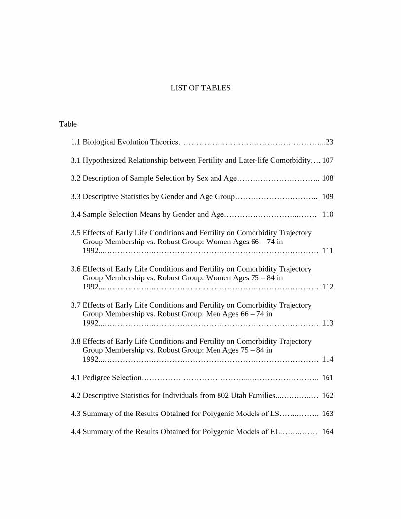
LIST OF TABLES
Table
1.1 Biological Evolution Theories………………………………………………... 23
3.1 Hypothesized Relationship between Fertility and Later-life Comorbidity…. 107
3.2 Description of Sample Selection by Sex and Age………………………….. 108
3.3 Descriptive Statistics by Gender and Age Group………………………….. 109
3.4 Sample Selection Means by Gender and Age………………………..……. 110
3.5 Effects of Early Life Conditions and Fertility on Comorbidity Trajectory
Group Membership vs. Robust Group: Women Ages 66 – 74 in
1992...……………….……………………………………………………… 111
3.6 Effects of Early Life Conditions and Fertility on Comorbidity Trajectory
Group Membership vs. Robust Group: Women Ages 75 – 84 in
1992...……………….……………………………………………………… 112
3.7 Effects of Early Life Conditions and Fertility on Comorbidity Trajectory
Group Membership vs. Robust Group: Men Ages 66 – 74 in
1992...……………….……………………………………………………… 113
3.8 Effects of Early Life Conditions and Fertility on Comorbidity Trajectory
Group Membership vs. Robust Group: Men Ages 75 – 84 in
1992...……………….……………………………………………………… 114
4.1 Pedigree Selection…………………………………....…………………….. 161
4.2 Descriptive Statistics for Individuals from 802 Utah Families...…….…..… 162
4.3 Summary of the Results Obtained for Polygenic Models of LS……..…….. 163
4.4 Summary of the Results Obtained for Polygenic Models of EL……..……. 164
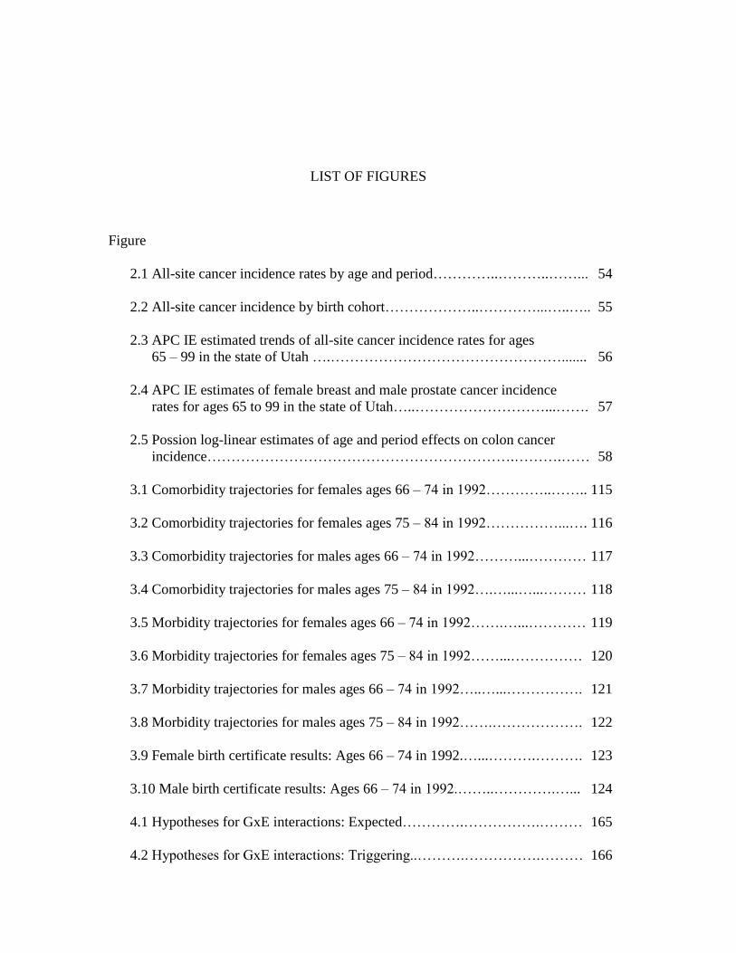
LIST OF FIGURES
Figure
2.1 All-site cancer incidence rates by age and period…………..………..……... 54
2.2 All-site cancer incidence by birth cohort………………..…………...…..….. 55
2.3 APC IE estimated trends of all-site cancer incidence rates for ages
65 – 99 in the state of Utah ….…………………………………………....... 56
2.4 APC IE estimates of female breast and male prostate cancer incidence
rates for ages 65 to 99 in the state of Utah…..………………………...……. 57
2.5 Possion log-linear estimates of age and period effects on colon cancer
incidence……………………………………………………….……….…… 58
3.1 Comorbidity trajectories for females ages 66 – 74 in 1992…………..…….. 115
3.2 Comorbidity trajectories for females ages 75 – 84 in 1992……………...…. 116
3.3 Comorbidity trajectories for males ages 66 – 74 in 1992………...………… 117
3.4 Comorbidity trajectories for males ages 75 – 84 in 1992….…...…...……… 118
3.5 Morbidity trajectories for females ages 66 – 74 in 1992…….…...………… 119
3.6 Morbidity trajectories for females ages 75 – 84 in 1992……...…………… 120
3.7 Morbidity trajectories for males ages 66 – 74 in 1992…..…...……………. 121
3.8 Morbidity trajectories for males ages 75 – 84 in 1992…….………………. 122
3.9 Female birth certificate results: Ages 66 – 74 in 1992.…...……….………. 123
3.10 Male birth certificate results: Ages 66 – 74 in 1992.……..………….…... 124
4.1 Hypotheses for GxE interactions: Expected………….…………….……… 165
4.2 Hypotheses for GxE interactions: Triggering..……….…………….……… 166

4.3 Hypotheses for GxE interactions: Compensation...….…………….……… 167
4.4 Hypotheses for GxE interactions: Enhancement.…….…………….……… 168
4.5 Predicted values of survival to the 50th
and 90th
percentiles by gender
and birth year………………………………….…………………………. 169
4.6 Distribution of calculated longevity for individuals born between 1850
and 1927 and surviving to age 30……….….……………………………. 170
4.7 Distribution of longevity by environment………………………………… 171
viii

CHAPTER 1
AGING AND LONGEVITY: THE PAST AND FUTURE TRENDS
Introduction
Demographers, biologists, social scientists, geneticists, historians, and other
scientists have long embarked on the quest of uncovering the secrets of healthy aging and
longevity. While the fascination with longevity is not unique to this time period, the
rapid changes in life expectancy and population structure over the past century have
elevated the importance of understanding determinants of healthy aging and longevity.
The mortality profiles of the developed countries have especially undergone fundamental
transformations over the past century. Life-expectancy in these populations has increased
linearly by approximately 3 months per year for the past 160 years (Oeppen & Vaupel,
2002). Historically, these improvements have been largely due to improvements in
survival in infancy and childhood. While less recognized, death rates at older ages have
also greatly improved over the last half of the 20th
century (Vaupel et al., 1998).
Significant declines in fertility during the demographic transition combined with
gains in life expectancy past age 65 have led to population aging (rising proportions of
the population age 65 and older) and increased levels of old-age dependency. These
changes have had profound policy implications. It is estimated that the proportion of the

2
population age 65 years and older will increase from 12.3% in 2000 to 21.1% in 2050 in
the United States (Uhlenberg, 2005). The oldest old population (ages 85+) is projected to
more than triple from its current estimate of 5.7 million to 24 million by 2050 (Vincent,
Velkoff, & Bureau, 2010), making it the fastest growing segment of the population. The
rising proportions of the population above the age of 65, combined with increases in life
expectancy and current trends in mortality decline in the oldest age categories, have made
the determinants of longevity and healthy aging critical to understanding population
health. Aging research is an extremely important domain of population health, and its
significance will increase as the proportion of the population age 65 and older continues
to rise.
The biological and social factors that determine healthy aging and longevity, and
their interaction, are still not well understood. In the past, misconceptions about the
limits of life-span have led demographers to underestimate the rate of decline in old-age
mortality (Uhlenberg, 2005). Current projections suggest that if the present gains in life
expectancy continue, more than half of individuals born after 2000 will live to see their
100th
birthday (Christensen, Doblhammer, Rau, & Vaupel, 2009). Unfortunately, such
projections ignore the complex interactions of social and biological factors that determine
mortality.
This dissertation improves upon previous research by investigating the influence
of the social environment, biology, and heritability throughout the life course on healthy
aging and longevity. The studies presented in this manuscript seek to disentangle the
biological and temporal sources of trends in cancer incidence, investigate the possible
social and physiological effects of fertility history on comorbidity trajectories after age
65, and explore the heterogeneity in heritable components of total phenotypic variation in

3
longevity across early life family and social environments. A fuller understanding of
heterogeneity in patterns of aging and the factors throughout the life course that shape
them will lead to more accurate population prediction, identify at risk population that
may benefit from more effective public health interventions, and characterize the process
of aging in a diverse population.
A rigorous investigation into biological and social causes of healthy aging and
longevity at advanced ages requires a theoretical framework capable of assimilating
theories from multiple disciplines. Biodemography provides a multidisciplinary
synthesis of biological, evolutionary, social science, ecological, life history and
demographic theories and is primed to answer a range of questions including those about
both how and why humans age (Vasunilashorn & Crimmins, 2008). Over the past few
decades, demographers have broadened the focus of work in the demography of aging
from a population aging perspective (i.e., measures of change in population age
structure), to include a perspective that integrates health and biological explanations with
traditional demographic and social theories of aging to explain variations in health and
mortality within and between populations (Olshansky, Carnes, & Brody, 2002; Siegel,
2011; Vasunilashorn & Crimmins, 2008).
The Biodemographic Perspective of Aging
As developed countries began to recognize most of the longevity gains to be
secured were achieved by improving infant and childhood mortality, questions began to
surface about how much improvement can be made in mortality rates at the other end of
the spectrum, what proportion of mortality at these ages is biologically determined, and
whether we are approaching a maximum life expectancy or linear gains can continued to

4
be realized (Carnes & Olshansky, 2007; Vaupel et al., 1998). “Aging, Natural Death, and
the Compression of Morbidity,” an article published by James Fries (1980), resulted in a
lively debate about the limits of life-span within the field of demography, with some
arguing that physiological decay was innately programmed (Fries, 1980), others
suggesting that old age is not biologically determined but there are practical limits that
will make steady improvements difficult (Carnes & Olshansky, 2007), and a third group
projecting linear increases in life expectancy for the foreseeable future (Vaupel et al.,
1998).
This debate is centered on a pivotal question; are we biologically programmed to
die? Even under ideal conditions, there is a progressive increase in age-specific death
rates and senescence (Carey & Judge, 2001). Theories aimed at answering why we
senesce and inevitably die can be classified into two broad categories: thermodynamic
and biological evolutionary theories of aging (Austad, 2001). Thermodynamic theories
implicitly or explicitly claim that aging is the inescapable consequence of the physical
nature of matter. These theories arrive at the conclusion that senescence is a genetically
programmed rate of decay, the natural consequence of approaching one’s maximum
possible life-span (Fries, 1980). Biological evolution theories explain senescence in
terms of selection forces acting on life history traits (Kirkwood & Rose, 1991).
Reliability theories of aging, optimization models, and nonadaptive mutation models (see
Table 1.1 for a more detailed description of these theories) all describe senescence as a
byproduct of evolution and not an innately programmed switch that is common to all
organisms.
The compression of morbidity hypothesis (Fries, 1980) argues that morbidity and
disability can be compressed to shorter periods toward the end of the life-span through

5
primary prevention such as maintaining a healthy lifestyle. Principally, he argued that
the rectangularization of the survival curve would be accompanied by an increase in age
at onset for chronic disease and disability which, in turn, compresses the time spent in a
diseased or disabled state. Others argued the failure of success hypothesis, which
suggests that improved survival of frail individuals will lead to increases in disease later
in life (Gruenberg, 1977; Kramer, 1980). Not only did these hypotheses spark interest in
determinants of life-span, but they also led to debate about heterogeneity in patterns of
aging, whether increased life expectancy indicated increased healthy life expectancy, and
whether centenarians escaped major age-related diseases.
The evidence consistent with morbidity compression is still uncertain. Most
evidence for individuals younger than 85 suggests there has been a postponement in
disease and disability over time, but little is known about trends in the population age
85+. This is largely because health data for this group of the population is not as readily
available (Boscoe, 2008). Although there are some studies of disease in centenarians that
suggest that a proportion of these exceptionally long-lived individuals delay or escape
disease, there is still considerable variation in disease experience (Andersen, Sebastiani,
Dworkis, Feldman, & Perls, 2012; Evert, Lawler, Bogan, & Perls, 2003). Uncertainty of
the expected trends in morbidity with age coupled with the fiscal demands of the
Medicare program have made the question of morbidity patterns above age 65 a central
biodemographic question. While the association between morbidity and mortality is
complex and varies across populations and environments (Siegel, 2011), most
classifications of morbidity (for example, heart disease and dementia) lead to higher rates
of death (Vaupel, 2010). Therefore, a more complete understanding of the determinates

6
of major morbid conditions and how these factors change over time can yield better
predictions of morbidity and mortality trends at advanced ages.
In his 1980 paper, Fries made a prediction: life expectancy would not exceed 85
years. This prediction was quashed in 2007, when the average life-expectancy for
Japanese women reached 86 years (Christensen et al., 2009). The continued steady rise
in life expectancy suggests that if there is a fixed limit, we have not yet reached it. While
limits in life expectancy suggested by those supporting a biological limit to life-span have
been surpassed, Jean Calment’s documented life-span of 122 years has yet to be broken.
Therefore two questions still remain: are we biologically programmed to die, and what
patterns of disease can we expect to see if life expectancy continues to rise? While these
questions have important implications for future population projections, we cannot arrive
at a suitable answer unless we consider another component that has been largely ignored
up to this point in the discussion: the relationship between social context, healthy aging,
and longevity.
Aging does not take place in isolation. It is heavily influenced by our
environments. Understanding the interplay between social context and biological factors
is imperative to understanding and predicting future trends in aging and mortality. Social
and historical context must be considered when determining morbidity and mortality
trends within a population. For example, studies have suggested that age, period, and
cohort factors are all important factors that affect population trends in mortality (Preston
& Wang, 2006; Yang, 2008). Mortality at ages 80 years and above has fallen at an
unprecedented pace since the 1950s (Kannisto, 1996), but old-age mortality in the United
States has stagnated since 1980 (Rau, Soroko, Jasilionis, & Vaupel, 2008). Other authors
have also noted the potential flaws in predicting future trends in longevity without

7
considering the social and historical context which shapes it, and have suggested that the
rapid increase in obesity may lead to declines in life expectancy in the near future (Jay
Olshansky et al., 2005; Reither, Olshansky, & Yang, 2011). Accurate predictions of
health and mortality of the aged population requires an approach that crosses disciplinary
boundaries and integrates biological and sociological concepts.
Biodemographers embrace the view that sociological context affects healthy
aging and longevity, for not only do social theories explain the demographic transition
but the central idea that health and longevity is socially patterned is deeply rooted in the
sociological tradition (Berkman & Syme, 1979; House, Landis, & Umberson, 1988; Link
& Phelan, 1995; Wen, Browning, & Cagney, 2003; Wise, 2003). But by integrating
biological theories and measures with sociological theories, the field of biodemography
has great potential for making contributions that will improve public health by
considering how social, economic, behavioral, and psychological conditions “get under
the skin” to cause health problems (Crimmins & Seeman, 2004; Robine, 2006;
Vasunilashorn & Crimmins, 2008). It has also become evident that proximate social
circumstances alone cannot explain heterogeneity in aging and the experiences across the
life course play an important role.
Biology, the Life Course, and Aging
Healthy aging and longevity cannot be understood by restricting analysis to a
single life stage because aging is a lifelong process. The life course perspective places
importance on both the historical and demographic parameters related to aging and
longevity, as well as the biological, social and psychological factors that influence aging
and longevity through direct (e.g., biological imprinting) and indirect (e.g., cumulative

8
and pathway) mechanisms throughout the life course (S. H. Preston, Hill, & Drevenstedt,
1998; Settersten, 2003). Simply put, it requires the researcher to consider how risk is
shaped throughout the life course, beginning with biological development in utero.
Genetic influences have been cited as perhaps the earliest biological factor
contributing to later life morbidity and mortality (Smith, Hanson, & Zimmer, 2012). The
two types of longevity genes, gerontogenes and longevity-assurance genes, can be used to
describe the effects of genes on longevity (Christensen, Johnson, & Vaupel, 2006;
Sebastiani et al., 2012). Gerontogenes negatively affect longevity, thus life-span
increases when their expression is blocked. Longevity assurance genes lead to a
phenotypic expression of longer life-span and therefore longevity decreases when their
expression is blocked. Thus, genetic endowments may either be protective, as in the case
of familial excess longevity (Smith, Mineau, Garibotti, & Kerber, 2009), or detrimental,
as in the case of certain apolipoprotein E (APOE) alleles (Ewbank, 2004).
Genes are fixed at birth, but is their expression? To answer this question,
comparisons of monozygotic and dizygotic twins have been made to compare life spans
while holding the childhood environment constant. These studies estimate heritability of
life-expectancy to be 25% (Herskind et al., 1996; Skytthe et al., 2003). Twin studies
have also revealed the variable nature of gene expression with age (Fraga et al., 2005;
Petronis et al., 2003) and it has been suggested that epigenetic mechanisms cause
individuals with the same genotype to have increasingly divergent phenotypes with age.
An individual’s genotype is inherited at birth and can be considered immutable.
However, gene expression is malleable because it is influenced by the environment
through the epigenome. Epigenetic modifications can be defined as “the sum of heritable
changes…that affect gene expression without changing DNA sequence” (Montesanto,

9
Dato, Bellizzi, Rose, & Passarino, 2012). Epigenetics is a bridge between genetics and
environment and may explain a portion of the variation in the rate of aging and longevity.
It is one of several possible biological mechanisms that allow social circumstances to get
“under the skin,” and epigenetic modifications have the propensity to persist across
subsequent generations (Feinberg, 2007). Differences in community and family
environments may affect the epigenetic regulation of gene expression and lead to
variation in the longevity phenotype. Recent studies suggest a relationship between
strength of genetic correlations and the quality and variability of an environment
(Charmantier & Garant, 2005). There may also be epigenetic changes in response to
individual social experiences throughout the life course (Champagne, 2010). Does the
social environment throughout the life course shape later life health and mortality?
Events throughout the life course can alter physiological functioning and affect
later life health and longevity. Early life conditions have been shown to be significantly
correlated with adult mortality for individuals and cohorts (Abel & Kruger, 2010; Barker,
1995; Doblhammer & Vaupel, 2001; Eriksson, Forsén, Tuomilehto, Osmond, & Barker,
2001). The fetal origins hypothesis and inflammation hypothesis are two theories that
have been used to explain the biological programming of an individual early in life.
According to the fetal origins hypothesis, individuals exposed to adverse conditions in
utero may have altered morbidity and mortality trajectories due to altered development of
key organ systems or epigenetic modifications during gestation. The inflammation
hypothesis argues that exposures to infectious disease during infancy and childhood
result in altered morbidity and mortality trajectories in adulthood (Crimmins & Finch,
2006; Finch & Crimmins, 2004). McDade, Rutherford, Adair, and Kuzawa (2010) have
proposed a related but alternative hypothesis predicting a negative relationship between
10
exposure to infectious disease and inflammation in adulthood, arguing that exposure to
infectious diseases are necessary for healthy development of the immune system.
Early life conditions may also be indirectly associated with morbidity and
mortality outcomes through correlated environments, cumulative processes, health
selection, and mortality selection. Indirect associations through correlated environments
are based on the principle of continuity of the life course and that one’s environment
during childhood is the same or similar to one’s adult environment. Selection
mechanisms may also lead to an indirect association between early life circumstances and
later life health outcomes. The health selection hypothesis argues that illness has social
consequences that may lead to poor socioeconomic status (SES) later in life and that it
may be the more proximate exposure to poor SES that is responsible for the observed
association between early life conditions and later life health (Montez & Hayward, 2011).
This continuity may lead to erroneously attributing the observed outcome to early life
conditions, when it is the proximate environment that is leading to adverse health
outcomes. Alternatively, genetic heterogeneity in the population may lead to differential
mortality selection; with those at the highest risk, the frail, being culled from the
population early leading to a population with a disproportionate representation of robust
individuals at older ages (Elo & Preston, 1992; Hawkes, Smith, & Blevins, 2012).
Related to this argument is the cumulative advantage/disadvantage hypothesis,
which argues that early life events can set into motion a trajectory where
advantage/disadvantage is accumulated throughout the life course (O'Rand & Hamil-
Luker, 2005). Sequential exposures to adverse environments may lead to excess stress or
exposure to chronic stress that leads to increased risk for disease later in life.
Conceptualizing aging and longevity as a lifelong processes allows for the study of how

11
inequalities are created through the accumulation of advantage/disadvantage across the
life course (Elder & Giele, 2009). Cumulative disadvantage can be set into motion by
early life events or situations that lead to structural constraints throughout the life course
(O'Rand & Hamil-Luker, 2005).
Physiological changes to the body in response to social conditions are not
constrained to critical or sensitive periods of development. These changes can occur in
response to prolonged exposure to stress throughout the life course. Allostatis, the ability
to achieve stability through change, is maintained in the body through the autonomic
nervous system, hypothalamic-pituitary-adrenal (HPA) axis, and the cardiovascular,
metabolic, and immune systems (McEwen, 1998). Allostatic load describes a process
through which exposure to chronic stress throughout the life course can lead to wear and
tear in these systems and lead to poor health in adulthood (Geronimus, 1992; McEwen,
1998), and these effects can be attenuated or accentuated by an individual’s access to
economic, social, or personal resources (Elder & Giele, 2009). Under this hypothesis,
individuals that are continually exposed to stress may experience physiological
deterioration of key systems that lead to chronic disease later in life. Recent epigenetic
research has also shown that epigenetic modifications occur across the life span
(Champagne, 2010; Montesanto et al., 2012; Shanahan & Hofer, 2011). While more
research needs to be done, it has been suggested that epigenetic changes during the aging
process may directly contribute to malignant transformation of cells (Fraga, 2009).
Placing human lives in context is fundamental to life course research. The life
course perspective promotes the view that social and physical environments vary by time
and space and underscores the multiple layers of human experience. It also highlights the
importance of historical change in determining health. These temporal changes in the

12
social or ecological environment are dependent upon the age of an individual and are
unique to a group of people born during the same time period or birth cohort.
Biodemography adds to this concept by recognizing that we live in a very different
environment from the one in which our life history evolved. Genetic, social, and
economic history and environments play an important role in shaping health and disease
patterns across populations and communities.
Birth cohorts are a measure of the social forces that shape health throughout the
life course (Keyes, Utz, Robinson, & Li, 2010). They vary in size, demographics, social
norms, prevalence of infectious disease, food availability, level of medical knowledge,
education, occupation, urbanization, etc., making each cohort unique. For example,
changes in smoking patterns or other environmental exposures over time may lead to
cohort specific trends in cancer incidence. They have been regarded as fundamental units
of social organization (Easterlin, 1998; Elder, 1999). Finch and Crimmins’ cohort
morbidity phenotype hypothesis suggests that differential exposure to infectious diseases
during childhood will lead to cohort differences in old age morbidity and mortality
(Crimmins & Finch, 2006; Finch & Crimmins, 2004). While cohort effects have proven
important for a number of different outcomes related to aging and longevity (Chen, Yang,
& Liu, 2010; Yang, 2008), some researchers are skeptical of the life course researcher’s
fascination with historical time (Fry, 2003), and others have argued that period factors
play a more important role in determining mortality rates in old age (Gagnon & Mazan,
2009; Kannisto, 1996).
The life course perspective facilitates questions about possible pathways to later
life health and potential confounding factors. The integration of biodemographic
principles and the life course framework could lend important insight into how the

13
heritability of longevity may be altered by events throughout the life course. Biological,
social, and psychological theories of development will be integrated in an attempt to
create a more complete view of how later life health is shaped by a lifetime of past
exposures.
Population aging is one of the greatest societal challenges of the next 50 years
(Kalache, Barreto, & Keller, 2005; Schoeni & Ofstedal, 2010). There are both social and
economic consequences of population aging. Accurate projections of how the elderly
population ages has policy implications for forecasting Social Security and Medicare
expenditures and predicting the costs of aging nationally and globally. The increase in
the proportion of the population over the age of 65 will also change the types of illnesses
and prevalent diseases in the population, affecting the types of medical services needed.
The projected increase in the proportion of the population at advanced ages has grave
implications for public pension programs, health care, and old age dependency. A greater
understanding of the sociological, biological, and heritable determinants of aging and
longevity is essential to maintaining a healthy population and economy.
The Determinants of Aging and Longevity
Perhaps the best way to elucidate mechanisms of aging and longevity is to study
the heterogeneity in morbidity and longevity and determine what factors contributed to
observed differences. This research contributes to the scientific understanding of aging
and longevity patterns and the factors throughout the life course that influence them.
Understanding the sources of variation in patterns of aging and longevity is important for
creating accurate population predictions, identifying at-risk populations that may benefit

14
from public health interventions, and characterizing the process of aging in a diverse
population.
Cancer was the second leading cause of death for individuals aged 65 and older in
the United States in 2010 (Miniño & Murphy, 2011), making it an essential component to
the study of aging and morbidity. Studies that do not account for changes in the
environment, diet, health behaviors, and screening and diagnostic practices are ignoring
the multifaceted determinants of cancer and may be inadvertently attributing temporal
determinates of observed trends to biological mechanisms. Failing to account for cohort
and period specific trends may confound the true age trajectory of cancer in this
population. Chapter 2 disentangles these trends for individuals age 65 to 99 using Utah
cancer incidence rates from 1963 to 2002, which lend better understanding to the true
age-specific trends in cancer incidence, including the previously understudied oldest old
age group (85+). It is important to account for cohort variations in aging and longevity in
order to avoid misattributing patterns caused by historical circumstances to biological
changes associated with age. Disentangling age, period, and cohort effects for major
health conditions in the oldest old categories will allow for more definitive assertions
about the possible causes of mortality deceleration and increased accuracy in forecasting
of future trends used to predict the fiscal burdens of an aging population.
The pathology of chronic disease is multifaceted, determined by genetic profiles,
biological and physiological development, and the social environment, with the strength
and relative importance of each of these factors varying throughout the life course.
Understanding longitudinal patterns of morbidity after age 65 is important to
understanding the mechanisms of aging and longevity. Equally important is what

15
predicts the observed patterns. Are measures of fertility and reproductive health
associated with morbidity profiles later in life?
Biological, evolutionary, and social theories all predict a relationship between
fertility and later life morbidity trajectories. Chapter 3 examines the role of parity, young
age at first birth, age at last birth, interbirth intervals, infant death, multiple births (twins),
marital status at time of birth, birth weight of offspring, and preterm births for both men
and women on disease progression after age 65. This study utilizes Centers for Medicare
(CMS) data spanning from 1992 – 2009 linked to the Utah Population Database, which is
a rich source of longitudinal data. Studying the effects of fertility history on men and
women at several stages in the aging process will lend clues to biological, evolutionary,
and social mechanisms that may lead to the observed outcomes.
For a more complete understanding of population heterogeneity in life-span and
the forces behind it, one must not only understand the average contribution of genes and
environment within a population toward explaining variation in adult mortality, but
uncover the factors that influence patterns of variation within the population. While there
is strong evidence supporting a genetic component to longevity, surprisingly, its size and
relative importance is poorly understood. Longevity is a complex trait, determined by a
multiplicity of genetic and environmental factors, with each factor contributing a
potentially small amount to phenotypic variation. This phenotypic variation can be
partitioned into genetic and environmental variation. Chapter 4 tests for heterogeneity in
the heritability of longevity across several early and midlife environments and explores
the possibility of gene-environment interactions (GxE). By examining sources of
variation in heritability estimates, we can illuminate factors that modify the expression of
genetic predisposition in a population. Understanding the role of biological and

16
environmental determinants of aging and mortality, and how they interact, can allow for
the identification of sources of variation in morbidity and mortality and improve
predictions of morbidity and mortality for future generations.
The final chapter provides a short summary of the findings from the studies
presented in Chapters 2-3. These studies provide insight into patterns and processes of
aging and highlight important factors to consider as the proportion of the population aged
65 years and older continues to grow. This chapter also gives direction for future
research and policy implications.
17
References
Abel, E. L., & Kruger, M. L. (2010). Birth month affects longevity. Death Studies, 34(8),
757-763.
Andersen, S. L., Sebastiani, P., Dworkis, D. A., Feldman, L., & Perls, T. T. (2012).
Health span approximates life span among many supercentenarians: Compression
of morbidity at the approximate limit of life span. The Journals of Gerontology
Series A: Biological Sciences and Medical Sciences, 67A(4), 395-405. doi:
10.1093/gerona/glr223
Austad, S. N. (2001). Concepts and theories of aging. In E. J. Masaro & S. N. Austad
(Eds.), Handbook of the biology of aging (Fifth ed., Vol. 1, pp. 3 - 18). United
States: Academic Press.
Barker, D. (1995). Fetal origins of coronary heart disease. BMJ, 311(6998), 171-174.
Berkman, L. F., & Syme, S. L. (1979). Social networks, host resistance, and mortality: A
nine-year follow-up study of Alameda County residents. American Journal of
Epidemiology, 109(2), 186-204.
Boscoe, F. P. (2008). Subdividing the age group of 85 years and older to improve US
disease reporting. American Journal of Public Health, 98(7), 1167.
Carey, J. R., & Judge, D. S. (2001). Principles of biodemography with special reference
to human longevity. Population: An English Selection, 13, 9-40.
Carnes, B. A., & Olshansky, S. J. (2007). A realist view of aging, mortality, and future
longevity. Population and Development Review, 33(2), 367-381.
Champagne, F. A. (2010). Epigenetic influence of social experiences across the lifespan.
Developmental Psychobiology, 52(4), 299-311. doi: 10.1002/dev.20436
Charmantier, A., & Garant, D. (2005). Environmental quality and evolutionary potential:
Lessons from wild populations. Proceedings of the Royal Society B: Biological
Sciences, 272(1571), 1415-1425. doi: 10.1098/rspb.2005.3117
Chen, F., Yang, Y., & Liu, G. (2010). Social change and socioeconomic disparities in
health over the life course in china. American Sociological Review, 75(1), 126-
150. doi: 10.1177/0003122409359165
Christensen, K., Doblhammer, G., Rau, R., & Vaupel, J. W. (2009). Ageing populations:
The challenges ahead. The Lancet, 374(9696), 1196-1208. doi:
http://dx.doi.org/10.1016/S0140-6736(09)61460-4
18
Christensen, K., Johnson, T. E., & Vaupel, J. W. (2006). The quest for genetic
determinants of human longevity: Challenges and insights. Nat Rev Genet, 7(6),
436-448.
Crimmins, E. M., & Finch, C. E. (2006). Infection, inflammation, height, and longevity.
Proceedings of the National Academy of Sciences of the United States of America,
103(2), 498-503. doi: 10.1073/pnas.0501470103
Crimmins, E. M., & Seeman, T. E. (2004). Integrating biology into the study of health
disparities. Population and Development Review, 30, 89-107.
Doblhammer, G., & Vaupel, J. W. (2001). Lifespan depends on month of birth. Proc Natl
Acad Sci U S A, 98(5), 2934-2939.
Easterlin, R. A. (1998). Growth triumphant: The twenty-first century in historical
perspective. Ann Arbor: Univ of Michigan Press.
Elder, G. H., & Giele, J. Z. (2009). The craft of life course research. New York: The
Guilford Press.
Elder, G. H. (1999). Children of the Great Depression: Social change in life experience:
Boulder, CO: Westview Press.
Elo, I. T., & Preston, S. H. (1992). Effects of early-life conditions on adult mortality: A
review. Population Index, 58(2), 186-212.
Eriksson, J., Forsén, T., Tuomilehto, J., Osmond, C., & Barker, D. (2001). Early growth
and coronary heart disease in later life: Longitudinal study. BMJ, 322(7292), 949-
953.
Evert, J., Lawler, E., Bogan, H., & Perls, T. (2003). Morbidity profiles of centenarians:
Survivors, delayers, and escapers. The Journals of Gerontology Series A:
Biological Sciences and Medical Sciences, 58(3), M232-M237. doi:
10.1093/gerona/58.3.M232
Ewbank, D. C. (2004). The APOE gene and differences in life expectancy in europe. The
Journals of Gerontology Series A: Biological Sciences and Medical Sciences,
59(1), B16-B20. doi: 10.1093/gerona/59.1.B16
Feinberg, A. P. (2007). Phenotypic plasticity and the epigenetics of human disease.
Nature, 447(7143), 433-440.
Finch, C. E., & Crimmins, E. M. (2004). Inflammatory exposure and historical changes
in human life-spans. Science, 305(5691), 1736-1739. doi:
10.1126/science.1092556

19
Fraga, M. F. (2009). Genetic and epigenetic regulation of aging. Current Opinion in
Immunology, 21(4), 446-453. doi: 10.1016/j.coi.2009.04.003
Fraga, M. F., Ballestar, E., Paz, M. F., Ropero, S., Setien, F., Ballestar, M. L., Heine-
Suner, D. et al. (2005). Epigenetic differences arise during the lifetime of
monozygotic twins. Proceedings of the National Academy of Sciences of the
United States of America, 102(30), 10604-10609. doi: 10.1073/pnas.0500398102
Fries, J. F. (1980). Aging, natural death, and the compression of morbidity. New England
Journal of Medicine, 303(3), 130-135.
Fry, C. L. (2003). The life course as a cultural construct. Invitation to the life course:
Toward new understandings of later life (pp. 269-294). New York: Baywood
Publising Company.
Gagnon, A., & Mazan, R. (2009). Does exposure to infectious diseases in infancy affect
old-age mortality? Evidence from a pre-industrial population. Social Science &
Medicine, 68(9), 1609-1616. doi: 10.1016/j.socscimed.2009.02.008
Geronimus, A. T. (1992). The weathering hypothesis and the health of African-American
women and infants: Evidence and speculations. Ethnicity & Disease, 2(3), 207.
Gruenberg, E. M. (1977). The failures of success. The Milbank Memorial Fund
Quarterly. Health and Society, 55(1), 3-24. doi: 10.2307/3349592
Hawkes, K., Smith, K. R., & Blevins, J. K. (2012). Human actuarial aging increases
faster when background death rates are lower: A consequence of differential
heterogeneity? Evolution, 66(1), s103-114.
Herskind, A., McGue, M., Holm, N., Sørensen, T., Harvald, B., & Vaupel, J. (1996). The
heritability of human longevity: A population-based study of 2872 Danish twin
pairs born 1870–1900. Human Genetics, 97(3), 319-323. doi:
10.1007/bf02185763
House, J., Landis, K., & Umberson, D. (1988). Social relationships and health. Science,
241(4865), 540-545. doi: 10.1126/science.3399889
Kalache, A., Barreto, S. M., & Keller, I. (2005). Global ageing: The demographic
revolution in all cultures and societies. The Cambridge Handbook of Age and
Ageing (pp.30, 606). Cambridge: Cambridge University Press.
Kannisto, V. (1996). The advancing frontier of survival: Life tables for old age (Vol. 3).
Odense, Denmark: Univ Press of Southern Denmark.
Keyes, K. M., Utz, R. L., Robinson, W., & Li, G. (2010). What is a cohort effect?
Comparison of three statistical methods for modeling cohort effects in obesity
20
prevalence in the United States, 1971–2006. Social Science & Medicine, 70(7),
1100-1108. doi: http://dx.doi.org/10.1016/j.socscimed.2009.12.018
Kirkwood, T. B. L., & Rose, M. R. (1991). Evolution of senescence: Late survival
sacrificed for reproduction. Philosophical Transactions of the Royal Society of
London. Series B: Biological Sciences, 332(1262), 15-24. doi:
10.1098/rstb.1991.0028
Kramer, M. (1980). The rising pandemic of mental disorders and associated chronic
diseases and disabilities. Acta Psychiatrica Scandinavica, 62(S285), 382-397. doi:
10.1111/j.1600-0447.1980.tb07714.x
Link, B. G., & Phelan, J. (1995). Social conditions as fundamental causes of disease.
Journal of Health and Social Behavior, 35, 80-94. doi: 10.2307/2626958
McDade, T. W., Rutherford, J., Adair, L., & Kuzawa, C. W. (2010). Early origins of
inflammation: Microbial exposures in infancy predict lower levels of C-reactive
protein in adulthood. Proceedings of the Royal Society B: Biological Sciences,
277(1684), 1129-1137. doi: 10.1098/rspb.2009.1795
McEwen, B. S. (1998). Protective and damaging effects of stress mediators. New
England journal of medicine, 338(3), 171-179. doi:
doi:10.1056/NEJM199801153380307
Miniño, A. M., & Murphy, S. L. (2011). Death in the United States, 2010. NCHS Data
Brief, 99 (pp. 1-8). Hyattsville, MD: National Center for Health Statistics. 2012
Montesanto, A., Dato, S., Bellizzi, D., Rose, G., & Passarino, G. (2012).
Epidemiological, genetic and epigenetic aspects of the research on healthy ageing
and longevity. Immun Ageing, 9(1), 6.
Montez, J. K., & Hayward, M. D. (2011). Early life conditions and later life mortality.
International handbook of adult mortality (pp. 187-206). New York: Springer.
O'Rand, A. M., & Hamil-Luker, J. (2005). Processes of cumulative adversity: Childhood
disadvantage and increased risk of heart attack across the life course. The
Journals of Gerontology Series B: Psychological Sciences and Social Sciences,
60(Special Issue 2), S117-S124.
Oeppen, J., & Vaupel, J. W. (2002). Broken limits to life expectancy. Science, 296(5570),
1029-1031. doi: 10.1126/science.1069675
Olshansky, S. J., Carnes, B. A., & Brody, J. (2002). A biodemographic interpretation of
life span. Population and Development Review, 28(3), 501-513.
Olshansky, S. J., Passaro, D. J., Hershow, R. C., Layden, J., Carnes, B. A., Brody, J.,
Hayflick, L., et. al. (2005). A potential decline in life expectancy in the United

21
States in the 21st century. New England Journal of Medicine, 352(11), 1138-
1145. doi: 10.1056/NEJMsr043743
Petronis, A., Gottesman, I. I., Kan, P., Kennedy, J. L., Basile, V. S., Paterson, A. D., &
Popendikyte, V. (2003). Monozygotic twins exhibit numerous epigenetic
differences: Clues to twin discordance? Schizophrenia Bulletin, 29(1), 169-178.
Preston, S. H., & Wang, H. (2006). Sex mortality differences in The United States: The
role of cohort smoking patterns. Demography, 43(4), 631-646. doi:
10.1353/dem.2006.0037
Preston, S. H., Hill, M. E., & Drevenstedt, G. L. (1998). Childhood conditions that
predict survival to advanced ages among African-Americans. Social Science &
Medicine (1982), 47(9), 1231.
Rau, R., Soroko, E., Jasilionis, D., & Vaupel, J. W. (2008). Continued reductions in
mortality at advanced ages. Population and Development Review, 34(4), 747-768.
doi: 10.1111/j.1728-4457.2008.00249.x
Reither, E. N., Olshansky, S. J., & Yang, Y. (2011). New forecasting methodology
indicates more disease and earlier mortality ahead for today’s younger Americans.
Health Affairs, 30(8), 1562-1568. doi: 10.1377/hlthaff.2011.0092
Robine, J. M. (2006). Research issues on human longevity. Human longevity, individual
life duration, and the growth of the oldest old population (pp. 7-42). Dordrecht:
Springer Netherlands.
Schoeni, R. F., & Ofstedal, M. B. (2010). Key themes in research on the demography of
aging. Demography, 47(1), S5-S15.
Sebastiani, P., Solovieff, N., DeWan, A. T., Walsh, K. M., Puca, A., Hartley, S. W.,
Melista, E., et. al. (2012). Genetic signatures of exceptional longevity in humans.
PLoS ONE, 7(1), e29848.
Settersten, R. A. (2003). Invitation to the life course: Toward new understandings of later
life. Amityville, NY: Baywood Publishing Company.
Shanahan, M. J., & Hofer, S. M. (2011). Molecular genetics, aging, and well-being:
Sensitive period, accumulation, and pathway models. Handbook of aging and the
social sciences (pp. 135-148). New York: Elsevier.
Siegel, J. S. (2011). The demography and epidemiology of human health and aging. New
York: Springer.
Skytthe, A., Pedersen, N. L., Kaprio, J., Stazi, M. A., Hjelmborg, J. v. B., Iachine, I.,
Vaupel, J. W.. et. al. (2003). Longevity studies in GenomEUtwin. Twin Research,
6(5), 448-454. doi: 10.1375/136905203770326457

22
Smith, K. R., Hanson, H. A., & Zimmer, Z. (2012). Early life conditions and later life
(65+) co-morbidity trajectories: The Utah Population Database linked to Medicare
claims data. Paper presented at the Population Association of America 2012, San
Fransico, CA.
Smith, K. R., Mineau, G. P., Garibotti, G., & Kerber, R. (2009). Effects of childhood and
middle-adulthood family conditions on later-life mortality: Evidence from the
Utah Population Database, 1850–2002. Social Science & Medicine, 68(9), 1649-
1658. doi: 10.1016/j.socscimed.2009.02.010
Uhlenberg, P. (2005). Demography of aging Handbook of population (pp. 143-167).
New York: Springer.
Vasunilashorn, S., & Crimmins, E. (2008). Biodemography: Integrating disciplines to
explain aging. Handbook of theories of aging (pp. 63-85). New York: Springer.
Vaupel, J. W. (2010). Biodemography of human ageing. Nature, 464(7288), 536-542.
Vaupel, J. W., Carey, J. R., Christensen, K., Johnson, T. E., Yashin, A. I., Holm, N. V.,
Iachine, I. A., et. al. (1998). Biodemographic trajectories of longevity. Science,
280(5365), 855-860. doi: 10.1126/science.280.5365.855
Vincent, G. K., Velkoff, V. A., & Bureau, U. C. (2010). The next four decades: The older
population in the United States: 2010 to 2050. US Dept. of Commerce,
Economics and Statistics Administration, US Census Bureau.
Wen, M., Browning, C. R., & Cagney, K. A. (2003). Poverty, affluence, and income
inequality: Neighborhood economic structure and its implications for health.
Social Science & Medicine (1982), 57(5), 843-860. doi: 10.1016/s0277-
9536(02)00457-4
Wise, P. H. (2003). The anatomy of a disparity in infant mortality. Annual Review of
Public Health, 24, 341-362. doi: 10.1146/annurev.publhealth.24.100901.140816
Yang, Y. (2008). Trends in U.S. adult chronic disease mortality, 1960–1999: Age, period,
and cohort variations. Demography, 45(2), 387-416. doi: 10.1353/dem.0.0000

Table 1.1 Biological Evolution Theories
(Adapted from Kirkwood 1991)
23
CHAPTER 2
AN AGE-PERIOD-COHORT ANALYSIS OF CANCER INCIDENCE
AMONG THE OLDEST OLD1
Abstract
Disentangling age, period, and cohort effects for major health conditions in the
oldest old categories will lead to better population projections of morbidity and mortality.
Data from the Utah Cancer Registry (UCR), the U.S. Census, the National Center for
Health Statistics (NCHS) and the National Cancer Institute’s Surveillence Epidemiology
and End Results (SEER) program are used to generate age-specific estimates of cancer
incidence for ages 65–99 from 1973–2002 for Utah. Age-period-cohort (APC) analyses
are used to describe the simultaneous effects of age, period and cohort on cancer
incidence rates in an attempt to understand the population dynamics underlying their
patterns. Our results show increasing cancer incidence rates up to the 85–89 age group
1 Accepted for publication in Population Studies. Coauthored by Ken R. Smith,
Antoinette M. Stroup, and C. Janna Harrell. Research was supported by the Utah Cancer
Registry (Contract No. HHSN261201000026C from the National Cancer Institute's
SEER Program) and NIA grant “Early Life Conditions, Survival, and Health”
(RO1AG022095, Smith PI) with additional support from the Utah State Department of
Health and the University of Utah. We would also like to acknowledge Ruldoph Rull and
Karim Al-Khafaji for their invaluable assistance with this project.

25
followed by declines for ages 90–99 net of period and cohort effects. We find significant
period and cohort effects, suggesting the role of environmental mechanisms in cancer
incidence trends between the ages of 85 and 100.
Introduction
The demographic profile of the United States is changing, with proportionately
more individuals surviving to very old ages. The oldest old population (ages 85+) is
projected to more than triple from its current estimate of 5.7 million to 24 million by
2050 (Vincent, Velkoff, & Bureau, 2010), making it the fastest growing segment of the
population. This substantial growth makes the study of morbidity and mortality for this
age group increasingly important.
The deceleration of all-site mortality at advanced ages is a commonly observed
phenomenon in both humans and animal species (Horiuchi & Wilmoth, 1998; Vaupel et
al., 1998) andcan be explained at the macrolevel due to changes in population
composition (e.g., heterogeneity hypothesis) or at the microlevel attributable to
physiological changes related to aging, (e.g., individual risk hypothesis). Alternatively,
this observed trend may be the result of age misreporting in the oldest age categories,
heterogeneous birth cohorts, and inaccurate measures of mortality in the oldest age
categories (Gavrilov & Gavrilova, 2011). While the association between morbidity and
mortality is complex (Siegel, 2011), studying patterns of human morbidity gives insight
into the age related changes in morbidity and mortality (Svetlana V. Ukraintseva &
Yashin, 2001), particularly for prevalent diseases such as cancer. A more complete
understanding of the determinates of cancer and how these factors change over time can
yield better predictions of morbidity and mortality trends at advanced ages.

26
Disentangling age, period, and cohort effects for major health conditions in the oldest old
categories will allow for more definitive assertions about the possible causes of mortality
deceleration and increased accuracy in forecasting of future trends used to predict the
fiscal burdens of an aging population.
Little is known about age-specific disease incidence and prevalence among the
oldest old, including cancer (Boscoe, 2008). In 2000, the oldest old age group accounted
for 8% of all incident cancer cases, and this number is projected to rise to 17% by 2050
assuming current incidence rates continue (Hayat, Howlader, Reichman, & Edwards,
2007). Unfortunately, traditional surveillance methods limit our ability to examine age-
specific cancer incidence in this subpopulation. The National Cancer Institute’s
Surveillance Epidemiology and End Results (SEER) program aggregates cancer
incidence information for the 85+ age group, making it difficult to study cancer trends in
the oldest old.
The few studies that examine cancer incidence trends after age 85 present
evidence of a deceleration in cancer incidence, prevalence, and mortality at the oldest
ages. (C. Harding, Pompei, Lee, & Wilson, 2008; Kaplan & Saltzstein, 2005; Saltzstein,
Behling, & Baergen, 1998). While patterns for different time periods are presented for
the oldest old population, the literature is limited with regard to analyzing change in the
trends over time. Time is a dimension of context, or the structure of the physical and
social environment related to a specific period or historical experiences unique to a birth
cohort, that influences health (Suzuki, 2012). Recent studies have shown the importance
of considering not only the effect of age, but also the role of period and cohort
experiences when studying health outcomes (Reither, Hauser, & Yang, 2009; Yang,
2008). Sex-specific trends in both all-site and site-specific cancer also need to be

27
considered because there may be different biological and social determinants of cancer
for men and women that vary by site (Yancik, 2005). This study aims to contribute to the
current literature by examining age, period, and cohort trends in cancer incidence from
1973 to 2002 for ages 65 to 99 using data from the Utah Cancer Registry (UCR), the
National Cancer Institute’s Surveillance, Epidemiology and End-Results Program
(SEER), the decennial Census, and the National Center for Health Statistics (NCHS).
Background
Disentangling Age, Period, and Cohort Effects
Age effects are generally understood to represent the biological characteristics of
an individual. Cross-sectional studies of all-site cancer incidence and death rates show
that rates generally increase with age, peaking between ages 75 and 85, and then
plateauing before declining in advanced ages (Andersen et al., 2005; Arbeev,
Ukraintseva, Arbeeva, & Yashin, 2005a; C. Harding et al., 2008; Saltzstein et al., 1998;
Stanta, 1997). However, many of these studies can only offer limited conclusions about
cancer trends in the oldest old because they aggregated ages 85+, examined a single
period, or failed to consider period and cohort influences.
Period effects can be described as the social and environmental context that
modifies risk for all individuals in a population at a specific point in time. Changes in
cancer screening technology may affect cancer incidence rates at all ages.
Mammography screening became widespread during the 1980s, leading to an increase in
incident female breast cancer diagnoses over the age of 65 (Edwards et al., 2002); colon
cancer cases increased during the 1990s as a result of changes in colorectal screening
(Edwards et al., 2002); and, there was a steep increase in incident prostate cancer cases

28
for males over the age of 65 between 1988 and 1992 due to the introduction of the
Prostate-Specific Antigen (PSA) screening test for prostate cancer (Edwards et al., 2002).
Changes in health care policy may also create period effects in cancer incidence. For
example, Medicare began covering mammographies in 1991(Kelaher & Stellman, 2000)
and colon cancer screening in 2001 (Berkowitz, Hawkins, Peipins, White, & Nadel,
2008). Thus, the introduction of new diagnostic tools into the health care market, and
changes in screening policies and medical practices have an impact on incidence rates
over time.
Cohort effects describe the social or ecological environment unique to individuals
born in the same group of years. Epidemiologists often describe cohort effects as the
interaction between age and period, while sociologists conceptualize them as a measure
of social forces that shape health throughout the life course (Keyes, Utz, Robinson, & Li,
2010). For example, changes in smoking patterns or other environmental exposures over
time may lead to cohort specific trends in cancer incidence. Improvement in cancer
screening technology may also have differential effects by birth cohort because the
benefit is not equally shared amongst all ages. For example, the Agency for Healthcare
Research and Quality does not recommend routine colonoscopies after the age of 75
(National Guideline), and questions about the efficacy of cancer screening for the oldest
old have also been raised (Østbye, Greenberg, Taylor, & Lee, 2003). In addition to the
age-based bias created by cancer screening recommendations, cancer incidence rates for
these ages may be subject to detection bias because screening is difficult for frail
individuals (Ukraintseva & Yashin, 2003). A more comprehensive understanding of the
age, period, and cohort factors contributing to cancer incidence rates in the oldest old is

29
essential for developing effective screening and treatment recommendations for this
population.
Cross-sectional analyses show a decline in cancer incidence for the oldest old that
is similar for men and women. However, results from previous studies indicate that the
shape, height, and peak of age-specific incidence curves are sensitive to both historical
period, cancer site, and study (C. Harding et al., 2008; Kaplan & Saltzstein, 2005;
Saltzstein et al., 1998). If cancer incidence rates in this age group were based strictly on
the biological factors contributing to aging, one would expect to see consistency in age-
specific rates over multiple periods of study. However, the fluctuation in rates is
evidence of the influence of external factors, related to period and birth cohort,
contributing to cancer incidence. Treating the pattern of decline as an effect of aging
neglects evidence of a social and ecological context that may alter age-specific trends and
ignores the multifaceted determinates of cancer risk (Kaplan & Saltzstein, 2005; Stanta,
1997). Using a comprehensive approach that studies cancer trends over time and
accounts for period and cohort effects will allow for a more accurate depiction of the age-
specific trends in cancer incidence.
Aging and Cancer
Disagreement exists among theories explaining the relationship between cancer
and aging and the observed decline in cancer incidence in the oldest old (Anisimov,
2003; Ukraintseva & Yashin, 2003). These controversies are similar to those surrounding
mortality deceleration and may prove useful for understanding the mechanisms driving
mortality deceleration.
30
There are three prevailing hypothesis explaining mortality deceleration (Gavrilov
& Gavrilova, 2011; Horiuchi & Wilmoth, 1998). The first hypothesis asserts that the
observed patterns of mortality deceleration are the result of age-misreporting and/or
model misspecification (Gavrilov & Gavrilova, 2011), thereby suggesting that mortality
does not decelerate with age, but is a statistical artifact. The other two hypotheses are the
heterogeneity hypothesis and the individual risk hypothesis (Horiuchi & Wilmoth, 1998).
These hypotheses lead to similar predictions about age related changes in cancer
incidence.
Theories Predicting that an Individual’s Cancer Risk Increases
with Age (Deceleration is an Artifact)
The multistage theory predicts that cancer incidence rates should increase with
age because the neoplastic transformation of cells occurs through several successive steps
(Anisimov, 2003; Armitage & Doll, 1954). This framework describes cancer incidence
as a power function of exposure time rather than age because cancer is caused by the dose
and duration of carcinogenic exposure over a person’s lifetime (Anisimov, 2003;
Ukraintseva & Yashin, 2003). Under this scheme, the path to cancer is step-wise and
irreversible, with each step leading to an increased probability of malignant
transformation with exposure time and therefore age. However, exposure risks between
cohorts may vary, giving rise to different patterns of age related incidence between birth
cohorts.
Physiological mechanisms may also explain increases of cancer incidence with
age. The cancer-longevity tradeoff hypothesis suggests that the cost of living a long life
is cancer. Physiological changes in the tissue microenvironment, telomere dysfunction,
31
a decline in immune surveillance, loss in tumor suppressor function, and mutation
accumulation are additional factors that have been cited as possible mechanisms leading
to the increasing rates of cancer incidence with age (Anisimov, 2003; Campisi, 2003;
Ukraintseva & Yashin, 2003). Many of these factors may be modified by environmental
exposures and therefore the context of time. Factors such as diet, smoking, exposure to
infectious disease (Ukraintseva & Yashin, 2003); and environmental interventions such
as exercise, social support, and screening practices, may make age specific trends
sensitive to temporal context.
Theories Predicting that an Individual’s Cancer Risk Declines
with Age (Individual Risk Hypothesis)
The individual risk hypothesis argues that the deceleration in morbidity and
mortality rates at older ages can be explained in terms of physiology, evolution, and
health behaviors (Horiuchi & Wilmoth, 1998; Vaupel et al., 1998). Although
physiological mechanisms have been used to explain increasing cancer incidence with
age, they may also predict the opposite—that cancer incidence in the oldest old age
categories decelerate and decline. Physiological changes can contribute to the decline in
cancer incidence in the oldest old through age-related declines in rates of cellular
metabolism, suppression of tumor generation, and increased cellular doubling time
(Ukraintseva & Yashin, 2003).
Natural selection may also affect age related declines in cancer incidence.
Mutation accumulation theory argues that age-related declines in the force of natural
selection may result in an accumulation of mutations that result in an increase in
mortality beginning near the end of reproductive ages followed by mortality deceleration
32
in the oldest age categories (Horiuchi & Wilmoth, 1998). In addition, mechanisms which
may protect against cancer may increase longevity, suggesting that individuals in the
oldest old age groups may be less susceptible to cancer (Campisi, 2003).
Variation in age-related health behaviors could also explain a decrease in cancer
incidence in the oldest old age groups. Cancer trends periodically shift due to changes in
screening procedures and recommendations, but these period effects may not be equal
across all ages. Routine cancer screening has increased in the general population
(Edwards et al., 2002); however, studies have suggested that there is a decrease in
surveillance for the oldest old and an increase in misdiagnosed or unreported tumors
(Kaplan & Saltzstein, 2005; Stanta, 1997). These factors may lead to cohort specific
trends in cancer incidence.
Population Heterogeneity Leads to Decreased Rates of Cancer
Incidence in the Oldest Old (Heterogeneity Hypothesis).
Population heterogeneity, differential risk patterns within a population, can be the
result of both within and between cohort differences, making the context of cohort an
important consideration. Within a single cohort heterogeneity can occur because the
force of mortality may decrease at advanced ages (Horiuchi & Wilmoth, 1998), pointing
researchers to a selection hypothesis to explain the decline. According to these
hypotheses, there is differential selection in a heterogeneous population with the frail
being selected out of the population at earlier ages (Hawkes, Smith, & Blevins, 2012).
Individuals culled from the population may have a genetic or environmental
predisposition to cancer, leaving their robust counterparts to survive to the oldest ages
with a survival advantage that protects them from cancer. For example, individuals with

33
deleterious mutations, such as the BRCA1 mutation, have elevated cancer mortality rates
as compared to the general population, making them less likely to survive to advanced
ages (K. R. Smith, Hanson, Mineau, & Buys, 2011).
Population heterogeneity can also arise because different cohorts have
experienced different mortality schedules, environmental exposures, public health
initiatives (such as antismoking campaigns), and cancer screening recommendations. It
has been suggested that the multistage theory is correct, and a plateau or decline in cancer
incidence rates at old ages may reflect period and cohort trends (Yang, 2008). If
exposure to different carcinogens such as tobacco smoke, changes in diet, or other
environmental carcinogens, fluctuates over time the deceleration in incidence rates at the
oldest ages may reflect these changes rather than somatic aging per se. A decline or
deceleration in cancer trends in old ages may be a function of cohort experiences such as
screening practices or health behaviors for this age group.
Understanding the relationship between cancer incidence and age will not only
improve future predictions of cancer incidence, it will help U.S. understand the
mechanisms leading to mortality deceleration in the oldest old population. Cancer trends
for the oldest old population are understudied because cancer incidence rates are
historically aggregated for all 85+ individuals (Boscoe, 2008). This study aims to
improve upon current literature by examining temporal trends of cancer incidence from
1973 to 2002 for ages 65 to 99.

34
Methods
Data
This study uses data for the state of Utah from 1973 to 2002 collected from the
Utah Cancer Registry (UCR), the National Cancer Institute’s Surveillance, Epidemiology
and End-Results Program (SEER), the decennial Census, and the National Center for
Health Statistics (NCHS). Cancer incidence cases and the U.S. Census Bureau’s
Population Estimates for the state of Utah for ages 65 to 84 were obtained from
SEER*Stat software (2010; 2012). Statewide cancer data are collected by the UCR as
part of routine cancer surveillance for the Utah Department of Health and the National
Cancer Institute’s SEER Program. Cancer cases are reported to the UCR through health
service providers and death certificates on which cancer is listed as a cause of death. Site
and histology are coded according to the International Classification of Diseases for
Oncology (ICD-O) at the time of diagnosis (Stroup, Dibble, & Harrell, 2008).
Age-specific incidence counts for ages 85 to 99 are not reported by the SEER
program. At these ages, age misstatement is a widely recognized problem, making
population estimates less reliable (Boscoe, 2008). Tabulated incidence data by year and
age were provided by the UCR. Intercensal population estimates were calculated via the
cohort-component and extinct-cohort methods using decennial data from the U.S. Census
Bureau and mortality data from the National Center for Health Statistics (Shryock,
Siegel, & Larmon, 1980). The cohort-component method starts with the cohort
populations reported in the decennial census and then subtracts deaths to estimate
population sizes. The use of census and death certificate data has been criticized because
upward age-misstatement can lead to a downward bias of incidence rates for this
population. However, age misstatement has been shown to be a relatively rare

35
occurrence with error rates improving over time (Boscoe, 2008; Hill, Preston, &
Rosenwaike, 2000; SH Preston, Stewart, & Elo, 1999). Data collection issues have also
caused errors in population estimates for the oldest old (Siegel & Passel, 1976). The
extinct-cohort method is an alternative method of calculating population counts. It relies
on death certificate data and is thought to be more reliable when cohorts are close to
extinction because it is less subject to bias caused by age misreporting. Rates from both
methods were compared and we found that when cohorts are farther from extinction
estimates using the extinct-cohort method become less reliable. The cohort component
method was selected as the basis for the final models. A detailed description of the
methods and comparison between rates will be presented in an article by Rudy et al. and
can be provided upon request. The final data set consisted of population level cancer
incidence counts (numerators) and cohort-component population estimates
(denominators) for the 65 to 99 year old Utah population from 1973 to 2002 by sex.
Statistical Methods
Sex- and site-specific cancer incidence trends from 1973-2002 for ages 65 to 99
for the state of Utah were selected for analysis. There were no incidence cases above age
100 from 1973 – 1982 and 1988 – 1997 for males and 1973 – 1977 for females; therefore
we did not include this age category in the analysis. Cancer incidence rates were
calculated as the ratio of incident cases to person years of exposure. Age-specific
incidence rates were tabulated in age a by calendar year period p arrays with diagonal
elements of the matrix corresponding to the birth cohorts c (c = p + a -1), where the
oldest cohort is observed for the oldest age interval during the earliest calendar period
and the youngest cohort is observed for the youngest age interval during the latest

36
calendar period. Seven 5-year age groups, ranging from 65 – 69 to 95 – 99, and six 5-
year time periods, from 1973 – 1977 to 1998 – 2002 were used in the analysis. There is
some ambiguity in the measurement of cohorts because data are tabulated into 5-year age
and period groupings. For example, an individual age 69 in 1973 would have a birth year
of 1904 while an individual age 65 in 1978 would have a birth year of 1913. This yielded
12 successive ten year birth cohorts with midpoints ranging from 1878 – 1933, which
were used for the age, period, and cohort (APC) analyses.
Traditional APC analyses suffer from an “identification problem” resulting from
the linear dependency between age, period and cohort (c=a +p), precluding a unique
solution. This problem can be solved by imposing constraints to the model to allow for
an identifiable solution (Arbeev et al., 2005a; Arbeev, Ukraintseva, Arbeeva, & Yashin,
2005b; Carstensen, 2007; Yang, Fu, & Land, 2004). However, selection of the
constraint requires some a priori knowledge of the disease under investigation and
models are sensitive to the constraint selected. Other authors have suggested using a
proxy characteristic for cohort (O'Brien, 1989, 2000; O'Brien, Stockard, & Isaacson,
1999). However, cohort characteristics may not entirely explain cohort effects and the
residuals may still be confounded in the model estimates with age and period effects.
The Intrinsic Estimator (IE) proposed by Yang et al. (Yang et al., 2004; Yang,
Schulhofer‐Wohl, Fu, & Land, 2008) can also be viewed as a constrained approach;
however, it does not require a priori assumptions about the constraints. Other studies
have shown that the IE produces substantively meaningful and empirically valid results
(Yang et al., 2008), and the effects can be interpreted like conventional regression
coefficients (D. J. Harding, 2009). The limitations to this approach include the lack of a
simple explanation of its assumptions and the lack of a full investigation of its properties
37
(D. J. Harding, 2009; H. L. Smith, 2004). After initial estimations of a series of Poisson
log-linear models, we selected the IE to estimate the APC effects of cancer incidence
based on evidence of distinct age, period, and cohort effects and model fit.
Descriptive plots were produced by age group and sex for all-site, breast, colon,
and prostate cancers to assess the age, period, and cohort cancer incidence trends. Trends
in lung cancer incidence rates were not assessed as part of this analysis because the
incidence rates in Utah are very low (Jemal et al., 2008) and the case counts above age 85
were sparse. A similar approach to that used by Yang et al. (Yang et al., 2004; Yang et
al., 2008) was used to identify an appropriate model to analyze the temporal trends in all-
site and site-specific cancer incidence rates. A series of Poisson log-linear models were
estimated for each site and sex:
ln(mijk) = ln(cijk/nijk) = μ + αi + βj + γk (eq. 2.1)
where rateijk indexes the expected cancer incidence rate in cell (i, j, k); cijk indexes the
observed number of cancer incidence cases; nijk indexes the number of person years; µ
indexes the intercept of age adjusted mean rate; αi indexes the ith row age effect for i = 1,
. . . , a age groups; βj represents the jth column period effect for j =1, . . ., p periods; and
γk represents the kth diagonal cohort effect for k =1, . . ., (a + p -1) cohorts.
One-way models (a, p, or c), two factor models (ap, pc, ca) and IE models were
compared. Both descriptive analyses and model fit, based on the Akaike Information
Criterion (AIC), were used to select the final models. Full analyses are available upon
request. The log-linear regression coefficients, standard errors, and model fit were
computed using Stata 11. 2. Estimates of the full APC models using the IE approach and
the apc_ie.ado downloaded from the Stata command line. To test whether our findings

38
were sensitive to method of denominator construction, the final models were replicated
using denominators constructed using the extinct cohort method.
Results
To assess the variation in age-specific incidence by period a series of age-period
plots were created. Figure 2.1 shows the sex-specific age and period all-site cancer
incidence rate plots. Each panel displays the age-specific incidence trends by calendar
period, ranging from 1973 - 1978 to 1998 - 2002. The solid lines present the full 85+
age-specific rates and the dashed lines display the trend when cancer rates are top-coded
at age 85. These plots show that when rates are aggregated for the 85 plus age group,
specious conclusions about the age at which incidence rates peak may be drawn. These
plots indicate that for the vast majority of the periods, the age group with the highest
incidence rates can be found in the 85 to 89 age groups. The peak is then followed by a
leveling off or decline for the 90 to 94 and 95 to 99 age groups. These plots also show
that the trends are not stable over time. If the only factor influencing cancer incidence
trends were age, one would expect the age-specific curves for all periods to follow
similar trajectories. However, the plots show variation in the intercept (depicted for age
65 - 69), slope, and shape of the curve. There has been a steady increase in the level of
cancer incidence over time, with the most recent periods having the highest rates for a
majority of the age groups.
Age-cohort plots were created to assess the variation in the age trends by birth
cohort and sex. Figure 2.2 displays the variation in shape, slope, and peak in all-site
cancer incidence age trends by cohort for both males and females. We are unable to
observe a single cohort for the entire age range because we have data for a 30 year

39
window only, from 1973 - 2002. Age trends for the 1903 and 1908 cohorts have the
longest follow-up, with incidence calculated for ages 70 to 99 and 65 to 94, respectively.
There is less variation in the trend in age specific incidence rates between cohorts for
females as compared to males. The plots suggest that for men the peak in incidence is
moving to younger ages for more recent birth cohorts; however, these peaks coincide
with the expected rise in incidence that resulted from the PSA testing for prostate cancer.
There is a general increase in cancer incidence rates at younger ages for more recent
cohorts for both males and females. For both sexes, the largest differences in cancer
incidence occur at ages 90 – 99. The imprecision at advanced ages is partially a function
of decreased sample sizes. The age-period and age-cohort plots indicate period and
cohort factors may confound observed trends in age specific cancer incidence.
A series of Poisson log-linear and IE models were used to further investigate age,
period, and cohort effects. The goodness-of-fit statistics for the log linear models are
displayed in Table S1 in the online supplement. The IE model provided the best fit for
both male and female all-site cancer, female breast cancer, and prostate cancer incidence.
The fit statistics suggest weak cohort effects for women, with the IE model only
providing a slightly better fit than the age-period models for both all-site and breast
cancer incidence. The age-period model provided the best fit for both male and female
colon cancer incidence models.
Figure 2.3 shows the IE results for all-site cancer incidence by sex. The figure
shows an increase across ages in cancer incidence up to age 85. All-site cancer incidence
rates are the highest for the 85 to 89 age group net period and cohort effects for both
males and females. Female all-site incidence rates for ages 90 and above level off and
the estimated coefficients are not statistically significant. There is a steeper decline in the
40
all-site incidence rate for males after age 85; however, it is noteworthy that the estimated
coefficient for rates at age 90 (p=0.06) is still higher than the estimated rates for both the
60 to 64 and 65 to 69 age groups.
The period specific trends show that there has been a gradual increase in cancer
incidence over time. While this gradual increase in cancer incidence with time may be
indicative of changes in screening behaviors or environmental exposures, it may also be
an artifact of changes in cancer surveillance methods, with more complete identification
of cases recorded over time. The period effects for males are as expected based on the
descriptive analyses and the known increase in cancer incidence between 1988 and 1992,
which is attributable to shifts in prostate screening practices. The rates drop to pre-1988
levels in the next period and continue their decline into the 1998 – 2002 period.
Figure 2.3 also shows that there are moderate cohort effects for females. All-site
cancer incidence was significantly higher for the 1888 and 1893 birth cohorts and lower
for the 1928 birth cohort. The cohort effects for males resemble a trough, with slightly
elevated risk (albeit insignificant) for early cohorts, followed by a decline and leveling
off for the 1903 to 1917 birth cohorts, and ending with an increase that almost reaches the
height of the 1883 birth cohort.
Figure 2.4 displays the IE estimates for breast and prostate cancer. The age
effects for the site specific cancers are somewhat different than the all-sites trends. For
females, the highest level of breast cancer incidence and the only estimate significantly
different from zero, is found between the ages of 75 to 79 (p=0.03). The period effects
are similar to those observed in the all-site rates as there is a gradual increase in female
breast cancer incidence over time. Cohort effects play a small role in determining female
breast cancer incidence over age 65. The decline in breast cancer incidence for the 1928

41
birth cohort is somewhat consistent with previous studies that show a decline in breast
cancer incidence for the 1924 to 1938 birth cohorts (Lacey, Devesa, & Brinton, 2002).
The age effect for males steadily increases up to age 75 where it reaches a plateau
followed by a decline at age 90. Male prostate cancer incidence steadily increases up to
1988 and then sharply declines over time, again for reasons of PSA testing. Male cohorts
between 1898 and 1918 have slightly lower rates of prostate cancer incidence. A steady
rise in prostate cancer rates is seen in subsequent cohorts.
Figure 2.5 shows the estimated coefficients for the log-linear AP models of colon
cancer incidence. Fit statistics showed that the two-factor model provided the best fit for
colon cancer incidence, meaning that cohort effects can be constrained to zero. Fig. 2.5
indicates that there is a steady increase in colon cancer incidence with age up to age 85,
followed by a slight decline (albeit still significantly higher than the referent category of
65 – 69) at the advanced ages. The period trends show a slight elevation in colon cancer
incidence between 1983 and 1987 for females and between 1983 and 1992 for males as
compared to the sex specific incidence rates in 1973 – 1977.
To test the sensitivity of our findings, the final models were estimated using
denominators created using the extinct cohort method. The results did not substantively
change the findings presented and are not shown here.
Discussion
This study found evidence supporting hypotheses of an increase in all-site cancer
incidence up to ages 85-89 net period and cohort effects, followed by a modest decline up
to age 99. Although incidence appears to drop after age 90, the rates up to age 99 are still
higher than rates for individuals aged 65-74. This finding is supported by other studies
42
and highlights the importance of disaggregating cancer incidence rates for the oldest old
(C. Harding et al., 2008; D. W. E. Smith, 1996). We found evidence of period and cohort
effects influencing cancer trends, which highlights the importance of considering the
social factors that influence biology when studying cancer trends in this population. The
benefits of disaggregated estimates for the oldest old far outweigh the potential
challenges related to age misreporting. As more people reach these advance ages, it will
become increasingly important to understand the biological and social mechanisms
affecting cancer trends in the oldest old. These results answer Boscoe’s call for greater
specificity in age-specific data for the oldest old (Boscoe, 2008).
We conclude that the age, period, and cohort effects of site specific cancer
incidence varied by site and sex. Physiological mechanisms have been the primary
mechanisms used to explain the decline in incidence by other authors. Harding et al.
propose a simple senescence theory, claiming that increasing senescence reduces the
ability of cells to divide and limits cancer incidence in the oldest old population (C.
Harding et al., 2008; C. Harding, Pompei, & Wilson, 2012). Our results suggest that age
is not the only factor contributing to the decline in cancer incidence in the oldest old age
group. We are not arguing against a biological model of cancer decline, but we do
advocate a more inclusive theory that considers socio-environmental factors and
mortality selection, which may influence the age-specific trends.
For women, the gradual increase in all-site and breast cancer incidence over time
may be partially due to increased detection by mammographic screening (Edwards et al.,
2002) and improvements in data collection and classification. These trends in breast
cancer incidence are also consistent with previously reported trends in breast cancer (C.
Harding et al., 2008; Kaplan & Saltzstein, 2005; Saltzstein et al., 1998). For men, the
43
dramatic increase in cancer incidence up to the 1988 – 1992 period is consistent with
other studies of period trends in prostate cancer incidence (Edwards et al., 2002) and the
introduction of the PSA screening test. The clear period trends observed for both men
and women bring attention to the importance of understanding how period factors
influence cancer incidence.
In our study, cohort effects played a larger role for males than females and did not
affect colon cancer incidence rates. Our results show variations in cohort trends of
cancer incidence over time that coincide with changes in environmental exposure to
tobacco products. Birth cohort did not explain variation in incidence trends for all sites in
this study. The absence of a cohort trend in colon cancer incidence is inconsistent with
other studies of colon cancer trends (Chu, Tarone, Chow, Hankey, & Ries, 1994);
however, cancer mortality trends may reflect improvements in detection and treatment
that prevent colon cancer mortality but do not necessarily modify the risk of colon cancer
incidence (which was not reported in this study). Failing to account for heterogeneity
between cohorts may lead to erroneous conclusions about deceleration in trends where
none exists (Gavrilov & Gavrilova, 2011). We have shown that there is a difference in
cancer susceptibility between cohorts, but controlling for these differences does not alter
the conclusion that cancer incidence rates do not exponentially increase with age.
Heterogeneity within a birth cohort may also be an important mechanism driving
the deceleration and decline in cancer incidence in the oldest old. Declines in the force of
mortality at all ages may lead to increased population heterogeneity at old ages, thus
possibly cohorts of individuals with more susceptibility to cancer (Hawkes et al., 2012).
However, it is also possible that there is less within-cohort heterogeneity in more recent
birth cohorts. Lynch and Brown (2001), have found evidence of less variation in
44
population frailty in birth cohorts in more contemporary cohorts, suggesting that the
population is becoming more homogeneously robust (Lynch & Brown, 2001). If this is
true, then it is possible that cancer incidence rates will decline in the future. The gradual
increase in cancer incidence for males during more recent birth cohorts, reported here,
suggests changing cohort susceptibility to cancer, a position inconsistent with the
argument that populations shift to become more homogenously robust. While it is
difficult to separate the environmental factors from the changes in population
heterogeneity, this finding emphasizes the importance of both improved surveillance in
cancer trends for the oldest old and consideration of cohort effects when studying oldest
old cancer trends.
Variation in health and cancer screening behaviors with age may also explain the
decline in incidence and sex differences in period and cohort effects. Sex differences in
cohort experiences may reflect sex differences in the timing, prevalence, and frequency
of smoking; sex differences in environmental exposures to carcinogens in the work place;
or sex differences in other risky behaviors that are patterned by generational experiences.
For example, Preston and Wang (2006) have demonstrated the close relationship between
a cohort’s mortality trajectory and its history of cigarette smoking as well as sex
differences in smoking prevalence within the cohort. It is unlikely that between-cohort
variability or period specific shifts in health behaviors are strong determinants of the age-
specific trend in cancer incidence because incidence rates decline above age 90 when
controlling for cohort and period trends.
Screening bias is another individual level component that may reduce cancer
incidence for the oldest old. For example, there were strong period effects associated
with the introduction of PSA testing for males. The birth cohorts that would have been in

45
the oldest age categories at the time PSA testing was introduced have decreased cancer
incidence rates relative to those cohorts that would have been under the age of 85. This
finding emphasizes the importance of both improved surveillance in cancer trends for the
oldest as well as further investigation into the causes of cohort differences in cancer
incidence. Kaplan and Satlzstein note parallel downward sloping trends between breast
cancer screening and prevalence in the aged population (Kaplan & Saltzstein, 2005).
However, other studies not subject to screening bias show a similar trend (Stanta, 1997).
This study also suggests that screening bias may not be the reason for decreases in cancer
incidence with age. SEER data collection processes include checking death certificate
information. Any cancer occurrence contributing to the cause of death of an individual is
reported to the SEER registries. Only cancers that are not an underlying factor in the
death would be missed by the system, suggesting that detection bias is not a likely cause
in the observed decrease in cancer at advanced ages.
Our results differ slightly from previously reported trends in cancer incidence.
The estimated peak in incidence in the 85 – 89 age category for males and females is
higher than the Harding et al. (2008) estimates of 80. However, our results are consistent
with the peak observed by Saltzstein et al. (1998). There are three possible explanations
for the variation in the estimated peaks in age-specific incidence rates. First, previous
studies of age-specific cancer incidence in the oldest old age group have not considered
the role of period and cohort effects. Ignoring exogenous factors that may contribute to
cancer incidence oversimplifies the problem and leads to the age-specific incidence rates
that are confounded by period and cohort differences in cancer incidence. APC analyses
of cancer incidence may provide less biased estimates of the true relationship between
cancer and aging.

46
Second, the differences may be caused by error in the estimated denominators.
Preston et al. (1999) found that the difference between the correct population distribution
and one estimated with age overstatement increased with time (Preston et al., 1999). Any
difference between the estimated peak cancer incidence and the true peak cancer
incidence should be negative. If age-misstatement led U.S. to overestimate the size of the
oldest old population, then our estimate of a peak in incidence between the ages of 85 and
89 is conservative. Furthermore, because other studies have also used decennial census
data to construct their denominators (C. Harding et al., 2008; C. Harding et al., 2012), we
argue that this is not the reason for the observed differences in peak age-specific
incidence rates.
Third, while not directly assessed, our findings are suggestive of geographic
variation in cancer incidence trends given the difference in the estimated peak of cancer
incidence between our study and other U.S. studies of overlapping time periods (Harding
et al., 2008; Harding et al., 2012; Saltzstein et al., 1998). Regional differences in cancer
incidence trends may be attributable to differences in sociodemographic characteristics,
health beliefs, access to resources, reproductive characteristics, and exposure to
environmental carcinogens. Utah consistently has one of the lowest cancer incidence and
mortality rates in the U.S. for both males and females and the lowest rates of lung cancer
incidence and mortality (Jemal et al., 2008). However, Utah does not have low incidence
rates for all cancer sites. Age-adjusted prostate cancer incidence rates are higher in Utah
than the national averages (Stroup et al., 2008). More research should be done to
quantify geographic differences as it will provide valuable information about the social
forces shaping cancer incidence rates in these age groups.

47
There are several structural limitations to studying cancer trends in the oldest old
age groups. Use of clinical and death certificate diagnoses may lead to an underreporting
of trends in the oldest old (Kaplan & Saltzstein, 2005; Stanta, 1997). Trends calculated
using cancer registry and census data are subject to error because the reliability of age
estimates for individuals over the age of 85 may be questionable (Edwards et al., 2002;
Vincent et al., 2010). However, we used several different methods to create measures of
population size and found no substantive differences in the age, period, and cohort trends
in all-site cancer incidence.
There is not widespread consensus in the cause of the decline in cancer rates at
advanced ages because it has been largely understudied. This study contributes to the
current literature by providing estimates of cancer incidence for the 85+ population
within the broader context of period and cohort effects. This study supports the
individual risk hypothesis and mortality selection arguments that predict a deceleration in
incidence at advanced ages. Our findings do not support the position that deceleration is
an artifact of variability in morbidity profiles between cohorts, nor do they support
arguments that cancer incidence trends are strictly a function of biological mechanisms.
Studies utilizing an APC approach to the analysis of cancer trends may provide less
biased estimates of the relationship between cancer and aging and improve knowledge
about the role of biological and social influences that modify trends. The existence of
cohort and period effects also justifies the use of direct measures of the exogenous factors
contributing to cancer incidence. Future studies should evaluate the proportion of
variation in cancer incidence explained by direct measures of period influences and
cohort characteristics. Future studies should also investigate morbidity trends in other
major causes of death and explore the relationship between these trends and mortality

48
deceleration. We also show that there is variation in cancer incidence trends in the oldest
old population and reiterate the importance of treating this population as heterogeneous.
In order to gain a more comprehensive understanding of morbidity and mortality patterns
for this rapidly growing segment of the population, cancer incidence and U.S. Census
population estimates need to be disaggregated for the oldest old population.

49
References
Andersen, S. L., Terry, D. F., Wilcox, M. A., Babineau, T., Malek, K., & Perls, T. T.
(2005). Cancer in the oldest old. Mechanisms Of Ageing And Development,
126(2), 263-267.
Anisimov, V. N. (2003). The relationship between aging and carcinogenesis: A critical
appraisal. Critical Reviews In Oncology/Hematology, 45(3), 277-304.
Arbeev, K. G., Ukraintseva, S. V., Arbeeva, L. S., & Yashin, A. I. (2005a). Decline in
human cancer incidence rates at old ages: Age-period-cohort considerations.
Demographic Research, 12(11), 273-300.
Arbeev, K. G., Ukraintseva, S. V., Arbeeva, L. S., & Yashin, A. I. (2005b). Mathematical
models for human cancer incidence rates. Demographic Research, 12(10), 237-
260.
Armitage, P., & Doll, R. (1954). The age distribution of cancer and a multi-stage theory
of carcinogenesis. British Journal of Cancer, 8(1), 1.
Berkowitz, Z., Hawkins, N. A., Peipins, L. A., White, M. C., & Nadel, M. R. (2008).
Beliefs, risk perceptions, and gaps in knowledge as barriers to colorectal cancer
screening in older adults. Journal of the American Geriatrics Society, 56(2), 307-
314. doi: 10.1111/j.1532-5415.2007.01547.x
Boscoe, F. P. (2008). Subdividing the age group of 85 years and older to improve U.S.
disease reporting. American Journal of Public Health, 98(7), 1167-1170. doi:
10.2105/ajph.2008.133900
Campisi, J. (2003). Cancer and ageing: Rival demons? Nature Reviews Cancer, 3(5),
339-349.
Carstensen, B. (2007). Age-period-cohort models for the Lexis diagram. Statistics in
Medicine, 26(15), 3018-3045.
Chu, K. C., Tarone, R. E., Chow, W.-H., Hankey, B. F., & Ries, L. A. G. (1994).
Temporal patterns in colorectal cancer incidence, survival, and mortality from
1950 through 1990. Journal of the National Cancer Institute, 86(13), 997-1006.
doi: 10.1093/jnci/86.13.997
Edwards, B. K., Howe, H. L., Ries, L. A. G., Thun, M. J., Rosenberg, H. M., Yancik, R.,
Wingo, P., et. al. (2002). Annual report to the nation on the status of cancer,
1973–1999, featuring implications of age and aging on U.S. cancer burden.
Cancer, 94(10), 2766-2792.

50
Gavrilov, L. A., & Gavrilova, N. S. (2011). Mortality measurement at advanced ages: A
study of the Social Security Administration Death Master File. North American
Actuarial Journal: NAAJ, 15(3), 432.
Harding, C., Pompei, F., Lee, E. E., & Wilson, R. (2008). Cancer suppression at old age.
Cancer Research, 68(11), 4465.
Harding, C., Pompei, F., & Wilson, R. (2012). Peak and decline in cancer incidence,
mortality, and prevalence at old ages. Cancer, 118(5), 1371-1386.
Harding, D. J. (2009). Recent advances in age-period-cohort analysis. A commentary on
Dregan and Armstrong, and on Reither, Hauser and Yang. Social Science &
Medicine, 69(10), 1449-1451. doi:
http://dx.doi.org/10.1016/j.socscimed.2009.08.034
Hawkes, K., Smith, K. R., & Blevins, J. K. (2012). Human actuarial aging increases
faster when background death rates are lower: A consequence of differential
heterogeneity? Evolution, 66(1), s103-114.
Hayat, M. J., Howlader, N., Reichman, M. E., & Edwards, B. K. (2007). Cancer statistics,
trends, and multiple primary cancer analyses from the Surveillance,
Epidemiology, and End Results (SEER) program. The Oncologist, 12(1), 20-37.
doi: 10.1634/theoncologist.12-1-20
Hill, M., Preston, S., & Rosenwaike, I. (2000). Age reporting among white Americans
aged 85+: Results of a record linkage study. Demography, 37(2), 175-186. doi:
10.2307/2648119
Horiuchi, S., & Wilmoth, J. (1998). Deceleration in the age pattern of mortality at
olderages. Demography, 35(4), 391-412. doi: 10.2307/3004009
Jemal, A., Thun, M. J., Ries, L. A. G., Howe, H. L., Weir, H. K., Center, M. M., . . .
Edwards, B. K. (2008). Annual report to the nation on the status of cancer, 1975–
2005, featuring trends in lung cancer, tobacco use, and tobacco control. Journal of
the National Cancer Institute, 100(23), 1672-1694. doi: 10.1093/jnci/djn389
Kaplan, R. M., & Saltzstein, S. L. (2005). Reduced mammographic screening may
explain declines in breast carcinoma in older women. Journal of the American
Geriatrics Society, 53(5), 862-866.
Kelaher, M., & Stellman, J. M. (2000). The impact of medicare funding on the use of
mammography among older women: implications for improving access to
screening. Preventive Medicine, 31(6), 658-664. doi: 10.1006/pmed.2000.0759
Keyes, K. M., Utz, R. L., Robinson, W., & Li, G. (2010). What is a cohort effect?
Comparison of three statistical methods for modeling cohort effects in obesity
51
prevalence in the United States, 1971–2006. Social Science & Medicine, 70(7),
1100-1108. doi: http://dx.doi.org/10.1016/j.socscimed.2009.12.018
Lacey, J. V., Devesa, S. S., & Brinton, L. A. (2002). Recent trends in breast cancer
incidence and mortality. Environmental and Molecular Mutagenesis, 39(2-3), 82-
88. doi: 10.1002/em.10062
Lynch, S. M., & Brown, J. S. (2001). Reconsidering mortality compression and
deceleration: An alternative model of mortality rates. Demography, 38(1), 79-95.
National Guideline, C. Colorectal cancer screening clinical practice guideline. Retrieved
11/30/2011, from http://www.guideline.gov
O'Brien, R. M. (1989). Relative cohort size and age-specific crime rates: An age-period-
relative-cohort-size model. Criminology, 27(1), 57-78.
O'Brien, R. M. (2000). Age period cohort characteristic models. Social Science Research,
29(1), 123-139.
O'Brien, R. M., Stockard, J., & Isaacson, L. (1999). The enduring effects of cohort
characteristics on age-specific homicide rates, 1960-1995 1. American Journal of
Sociology, 104(4).
Østbye, T., Greenberg, G. N., Taylor, D. H., & Lee, A. M. M. (2003). Screening
mammography and pap tests among older american women 1996–2000: Results
from the Health and Retirement Study (HRS) and Asset and Health Dynamics
Among the Oldest Old (AHEAD). The Annals of Family Medicine, 1(4), 209-217.
doi: 10.1370/afm.54
Preston, S., Stewart, Q., & Elo, I. (1999). Effects of age misreporting on mortality
estimates at older ages. Population Studies, 53(2), 165-177.
Preston, S., & Wang, H. (2006). Sex mortality differences in the United States: The role
of cohort smoking patterns. Demography, 43(4), 631-646. doi:
10.1353/dem.2006.0037
Reither, E. N., Hauser, R. M., & Yang, Y. (2009). Do birth cohorts matter? Age-period-
cohort analyses of the obesity epidemic in the United States. Social Science &
Medicine, 69(10), 1439-1448. doi:
http://dx.doi.org/10.1016/j.socscimed.2009.08.040
Saltzstein, S. L., Behling, C. A., & Baergen, R. N. (1998). Features of cancer in
nonagenarians and centenarians. Journal of the American Geriatrics Society,
46(8), 994.
SEER*Stat Database: Incidence - SEER 9 Regs Research Data, Nov 2010 Sub (1973-
2008) <Katrina/Rita Population Adjustment> - Linked To County Attributes -
Total U.S., 1969-2009 Counties, National Cancer Institute, DCCPS, Surveillance

52
Research Program, Cancer Statistics Branch. (2010). Retrieved from:
www.seer.cancer.gov
SEER*Stat Database: Populations - Total U.S. (1969-2009) Single Ages to 85+,
Katrina/Rita Adjustment - Linked To County Attributes - Total U.S., 1969-2009
Counties, National Cancer Institute, DCCPS, Surveillance Research Program,
Cancer Statistics Branch, released April 2011. (2012). Retrieved from:
www.seer.cancer.gov
Shryock, H. S., Siegel, J. S., & Larmon, E. A. (1980). The methods and materials of
demography (Vol. 2): U.S. Dept. of Commerce, Bureau of the Census: For sale by
the Supt. of Docs. U.S. Govt. Print. Off.
Siegel, J. S. (2011). The demography and epidemiology of human health and aging: New
York: Springer.
Siegel, J. S., & Passel, J. S. (1976). New estimates of the number of centenarians in the
United States. Journal of the American Statistical Association, 559-566.
Smith, D. W. E. (1996). Cancer mortality at very old ages. Cancer, 77(7), 1367-1372.
Smith, H. L. (2004). Response: Cohort analysis redux. Sociological Methodology, 34(1),
111-119. doi: 10.1111/j.0081-1750.2004.00149.x
Smith, K. R., Hanson, H. A., Mineau, G. P., & Buys, S. S. (2011). Effects of BRCA1 and
BRCA2 mutations on female fertility. Proceedings of the Royal Society B:
Biological Sciences, 279(1732), 1389-1395.
Stanta, G. (1997). Cancer of the oldest old. What we have learned from autopsy studies.
Clinics in Geriatric Medicine, 13(1), 55.
Stroup, A. M., Dibble, R., & Harrell, C. T. R. C. J. (2008). Cancer incidence and
mortality trends in Utah: 1973-2004. UH Review 2008, 25.
Suzuki, E. (2012). Time changes, so do people. Social Science & Medicine, 75(3), 452-
456. doi: http://dx.doi.org/10.1016/j.socscimed.2012.03.036
Ukraintseva, S. V., & Yashin, A. I. (2001). How individual age-associated changes may
influence human morbidity and mortality patterns. Mechanisms of Ageing and
Development, 122(13), 1447-1460. doi: http://dx.doi.org/10.1016/S0047-
6374(01)00277-9
Ukraintseva, S. V., & Yashin, A. I. (2003). Individual aging and cancer risk: How are
they related. Demographic Research, 9(8), 163-196.

53
Vaupel, J. W., Carey, J. R., Christensen, K., Johnson, T. E., Yashin, A. I., Holm, N. V.,
Iachine, I. A. et. al. Curtsinger, J. W. (1998). Biodemographic trajectories of
longevity. Science, 280(5365), 855-860. doi: 10.1126/science.280.5365.855
Vincent, G. K., Velkoff, V. A., & Bureau, U. C. (2010). The next four decades: The older
population in the United States: 2010 to 2050: U.S. Dept. of Commerce,
Economics and Statistics Administration, U.S. Census Bureau.
Yancik, R. (2005). Population aging and cancer: A cross-national concern. The Cancer
Journal, 11(6), 437.
Yang, Y. (2008). Trends in U.S. adult chronic disease mortality, 1960-1999: Age, period,
and cohort variations. Demography, 45(2), 387-416.
Yang, Y., Fu, W. J., & Land, K. C. (2004). A methodological comparison of age‐period‐cohort models: The intrinsic estimator and conventional generalized linear
models. Sociological Methodology, 34(1), 75-110.
Yang, Y., Schulhofer‐Wohl, S., Fu, W. J., & Land, K. C. (2008). The intrinsic estimator
for age‐period‐cohort analysis: What it is and how to use it. American Journal of
Sociology, 113(6), 1697-1736.

54
Figure 2.1. All-site cancer incidence rates by age and period. Panels A and B show Utah
females and males, respectively. Solid lines show trends up to age 99 and dashed lines
show the trend when cancer incidence is aggregated for individuals 85 years and above.

55
Figure 2.2. All-site cancer incidence by birth cohort. Panels A and B show Utah females
and males, respectively. The scale of the y-axis is smaller than the scale for the male
graphs to allow for the visibility of the variation. Female incidence rates are lower
than male incidence rates and increase with age at a slower rate.
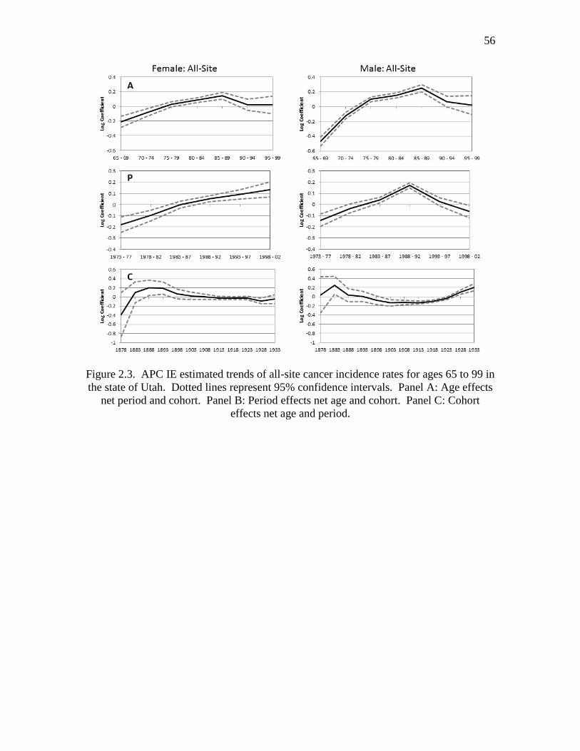
56
Figure 2.3. APC IE estimated trends of all-site cancer incidence rates for ages 65 to 99 in
the state of Utah. Dotted lines represent 95% confidence intervals. Panel A: Age effects
net period and cohort. Panel B: Period effects net age and cohort. Panel C: Cohort
effects net age and period.
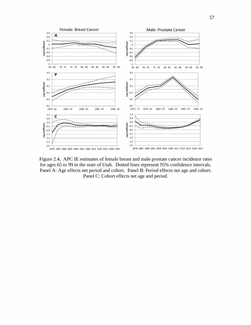
57
Figure 2.4. APC IE estimates of female breast and male prostate cancer incidence rates
for ages 65 to 99 in the state of Utah. Dotted lines represent 95% confidence intervals.
Panel A: Age effects net period and cohort. Panel B: Period effects net age and cohort.
Panel C: Cohort effects net age and period.
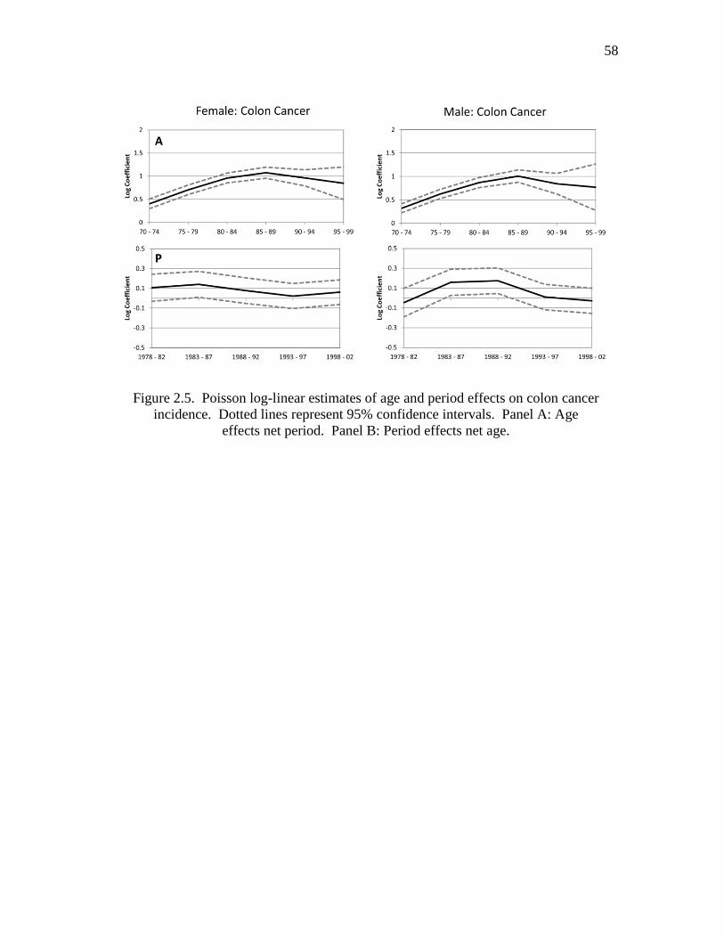
58
Figure 2.5. Poisson log-linear estimates of age and period effects on colon cancer
incidence. Dotted lines represent 95% confidence intervals. Panel A: Age
effects net period. Panel B: Period effects net age.

CHAPTER 3
REPRODUCTIVE HISTORY AND LATER-LIFE COMORBIDITY
TRAJECTORIES2
Abstract
The reproductive lives of men and women may provide significant insight into
later-life health and mortality. Sociological, biological, and evolutionary theories predict
a relationship between reproductive history and later-life health and mortality, however,
current research is lacking consensus on the direction of the relationship. In this study,
the relationship between reproductive history and later-life health is examined using data
based on linkages between the Utah Population Database, a rich source of longitudinal
data, and 18 years of Medicare Claims data. Later-life health is measured using the
Charlson Comorbidity Index, a construct that summarizes nearly all serious illnesses
afflicting older individuals. Single year comorbidity scores are constructed by year from
1992 to 2009. We used group based trajectory modeling that accounts for nonrandom
attrition due to death to identify the number and types of morbidity trajectories by sex
and age group for 52,924 individuals aged 65-84 in 1992. For both males and females,
2 Coauthored by Ken R. Smith and Zachary Zimmer. We wish to thank the Pedigree and
Population Resource of the Huntsman Cancer Institute, University of Utah for providing
the data and valuable computing support. This work was also supported by NIH grant
AG022095 (Early-life Conditions, Survival and Health; Smith PI).
60
trajectory groups ranged from a robust group with little to no comorbid conditions during
the period of observation to a frail group with a consistently high comorbidity. Parity,
age at first birth, age at last birth, birth weight of offspring, having a child die as an
infant, and having a preterm birth predicted trajectory group membership for women but
had little association with trajectory group membership for men.
Introduction
Understanding how individuals experience disease after age 65 is important to
understanding the mechanisms of aging and longevity. Equally important is what
predicts the observed patterns. The etiological model of chronic disease has shifted its
focus from adult risk factors to considering factors throughout the life course (Kuh &
Ben-Shlomo, 2004). Central to the life course approach is the idea that there are certain
periods of plasticity, where individuals may experience physiological or social change
that alter their future health trajectories. The reproductive period is a sensitive period for
both men and women, in which the timing of births, number of births, and birth outcomes
might have adverse or protective effects on later-life health. It also presents a critical
period for women as physiological changes related to pregnancy may have lifelong
effects on the structure or function systems in the body (Kuh & Ben-Shlomo, 2004; Kuh
& Hardy, 2002). Therefore, the reproductive lives of men and women may provide
significant insight into later-life health and mortality, but current research is lacking
consensus on the direction of the relationship.
This study will examine the role of parity, age at first birth, age at last birth,
interbirth intervals, infant death, multiple births (twins), birth weight of offspring, and
preterm births for both men and women on disease progression after age 65. This study

61
utilizes Centers for Medicare Services (CMS) data spanning from 1992 – 2009 linked to
the Utah Population Database, which is a rich source of longitudinal data. The goals of
this analysis are threefold: 1- identify distinct trajectories of comorbidity from 1992 -
2009 for individuals aged 66 – 84 in 1992 by sex and birth cohort; 2- estimate the
association between measures of fertility and later-life comorbidity trajectories while
controlling for early-life circumstances using information from a longitudinal, familial
health database; 3- determine if the observed effects are part of a trajectory set in motion
earlier during infancy and childhood (i.e., does fertility mediate known relationships
between early-life circumstances and later-life comorbidity trajectories (K. R. Smith,
Hanson, & Zimmer, 2012)).
Background
There is a substantial amount of variation in the morbidity profile of older adults,
suggesting that morbidity is not an inevitable consequence of aging (Rowe & Kahn,
1987; Rowe & Kahn, 1997). Understanding the sources of variation in patterns of aging
is important for creating accurate population predictions, identifying at risk populations
that may benefit from public health interventions, and characterizing the process of aging
in a diverse population. Sources of heterogeneity in patterns of aging cannot be
understood by restricting analyses to a single life stage, nor can its intricacies be
understood without simultaneously considering biological and social mechanisms. The
pathology of chronic disease is multifaceted, determined by genetic profiles, biological
and physiological development, and the social environment, with the strength and relative
importance of each of these factors varying throughout the life course.

62
The majority of studies assessing the relationship between reproductive history
and health have focused on mortality with mixed results. Numerous studies have also
demonstrated the relationship between reproductive history and later-life health as
measured by activities of daily living (ADL), depressive symptoms, type 2 diabetes,
cardiovascular disease, self-rated health, self-reported limiting chronic illness, cancer,
and mental health (D. Smith, Sterne, Tynelius, & Rasmussen, 2004; Grundy &
Tomassini, 2005; Henretta, 2008; Kravdal, 1995; Lawlor et al., 2003; Myklestad et al.,
2012; Spence, 2008; Yi & Vaupel, 2004). Yet none has looked at the relationship
between reproductive history and comorbidity. These studies also often fail to account
for early-life conditions that may influence reproductive history and later-life health.
Comorbidity is one of the major components of health aging, and its presence
increases with age (L. P. Fried, Ferrucci, Darer, Williamson, & Anderson, 2004;
Guralnik, 1996). However, there is variation in the rate at which a transition into a
comorbid state occurs and the trajectory of disease once it has occurred. We assume that
heterogeneity within a population follows a specific distribution, with robust individuals
on one tail and frail individuals on the other. Therefore, unlike the geriatric definition of
frailty which refers to a variable state of physiological decline, we intend to invoke the
demographic meaning of the term. For example, individuals exhibiting a robust
phenotype may delay or evade chronic disease completely, while individuals exhibiting
the frail phenotype experience multiple morbid conditions (Andersen, Sebastiani,
Dworkis, Feldman, & Perls, 2012; Evert, Lawler, Bogan, & Perls, 2003; Ken R. Smith et
al., 2012). Identifying sources of this phenotypic variation is necessary for targeting
periods of the life course that affect later-life health and to more fully understand the
process of aging. Preston, Hill, and Drevenstedt (1998) have proposed a widely used

63
model explaining the direct and indirect effects of childhood circumstances on later-life
health. A similar model can be used to classify the theories that predict a relationship
between fertility history and later-life health. Evolutionary, biological, and social
theories predict that parity, age at first birth, age at last birth, interbirth intervals,
twinning, birth weight of offspring, and giving birth prematurely may all be associated
with later-life morbidity and mortality.
Evolutionary and Genetic Theories Linking
Reproductive Health to Aging
Evolutionary theories predict a close relationship between fertility and mortality.
Optimization hypotheses suppose that the forces of evolution select for traits that
maximize the reproductive success of an organism. Two such hypotheses, disposable
soma and antagonistic pleiotrophy, predict a positive association between parity and
comorbidity at advanced ages (Kirkwood & Rose, 1991). The disposable soma theory
argues that the two physiological costly functions of reproduction and somatic
maintenance are in direct competition for a limited amount of resources. This “trade-off”
yields optimal reproductive success at the cost of longevity for females (Kirkwood &
Rose, 1991). Similarly, antagonistic pleiotrophy suggests that genetic mutations that
increase postreproductive mortality may escape the force of natural selection because
they increase fitness early on (Kirkwood & Rose, 1991; G. C. Williams, 1957). A recent
study of fertility in carriers of the breast cancer genes BRCA1 and BRCA2 suggests that,
although these mutations significantly increase the risk of mortality, they may increase
reproductive fitness and therefore have not been selected out of the population (K. R.

64
Smith, Hanson, Mineau, & Buys, 2012). These theories predict that for females, young
age at first birth and high parity are associated with increased comorbidity later in life.
High parity, late age at last birth, multiple births, and short birth intervals may
also be associated with decreased comorbidity later in life. For example, it has been
suggested that genetic variants influence both late female fertility and slowed rates of
somatic aging (K. R. Smith et al., 2009). Fertility success may also be an indication of
health status and robustness. Women with higher fertility, shorter birth intervals, twins,
and later ages at last birth may have increased longevity because their fertility success is
a marker of a robust phenotype (Hawkes, 2010; Robson & Smith, 2011, 2012). While
evolutionary theories are an important factor in the relationship between fertility and
later-life morbidity and mortality, it is necessary to consider the direct biological and
indirect social effects of fertility history.
Direct Biological Effects of Reproductive Health and
Biological Indicators of Later-Life Health
In the life course literature, physiological scarring has been used to define an
event that permanently alters the physiological functioning of an organism. For women,
pregnancy may trigger physiological changes that may favorably or adversely affect
later-life health. Increased parity and early age at first birth have been shown to lower
the risk of postmenopausal reproductive cancer and it has been posited that biological
factors are responsible for this link. Pregnancy is one of several factors that determine
life time exposure to endogenous hormones. Several hypotheses relate the level of
endogenous hormones throughout the life course, such as androgen, insulin,
progesterone, and estrogen, to cancer risk later in life (Kelsey, Gammon, & John, 1993;

65
Kobayashi et al., 2012; Lukanova & Kaaks, 2005). There is an inverse association
between parity and cancer incidence in tissues sensitive to hormone levels, such as breast,
endometrial and ovarian (Kelsey et al., 1993; Kobayashi et al., 2012; Kvale, Heuch, &
Nilssen, 1994; Permuth-Wey & Sellers, 2009). Age at first birth has also a known risk
factor for breast cancer, with younger age at first birth being a protective factor
(MacMahon, Cole, & Brown, 1973).
Reproductive history may also lead to physiological changes that adversely affect
a woman’s health. Pregnancy related biological responses may lead to increased risk for
coronary heart disease and obesity later in life (Bastian, West, Corcoran, & Munger,
2005; Lawlor et al., 2003). A study of men and women aged 60 to 79 in Britain found a
positive association between number of children and adverse lipid profiles and diabetes
for women but not men, suggesting possible biological mechanisms (Lawlor et al., 2003).
However, life style factors were also found to play a role in the association. Birth
spacing and having multiple births (twins) may also leave a physiological imprint on the
mother. The maternal depletion hypothesis argues that the physiological demands of
pregnancy diminish physical resources and short birth intervals do not give the mother
ample time to recover from the stresses of the previous pregnancy (Jelliffe & Jelliffe,
1978; Kirkwood & Rose, 1991). These theories predict a positive relationship between
parity, short birth intervals, and multiple births and later-life comorbidity.
Characteristics of a mother’s offspring at time of birth can be used to gauge the
woman’s health during her reproductive period and may predict her health status as she
ages. Birth weight of her child and giving birth prematurely are examples of markers of
the health and vitality of the mother (G. D. Smith, Whitley, Gissler, & Hemminki, 2000).
Giving birth to an infant that is considered large for its gestation age (LGA) may be an

66
indication of pregnancy complications that affect the mother’s health, such as gestational
diabetes (Casey, Lucas, McIntire, & Leveno, 1997), which is a known risk factor for
diabetes and cardiovascular disease later in life (Bellamy, Casas, Hingorani, & Williams,
2009; Carr et al., 2006). Studies have shown that there is a positive association between
birth weight of offspring and the mother’s longevity (G. D. Smith et al., 1997; G. D.
Smith et al., 2000). However, the studies do not test whether there is a threshold to this
effect. There are several reasons for these associations. First, it may be an indicator of
the social and physical environment of the mother, with conditions affecting the
development and health of both mother and fetus. Second, it may be indicative of genetic
variants carried by the mother or father that predispose them for cardiovascular disease
later in life (Myklestad et al., 2012). These studies suggest that high birth weight, low
birth weight, and preterm babies are positively associated with adverse health outcomes
later in life.
Social Mechanisms Indirectly Linking Reproductive
History to Later-Life Health
Social theories predict both positive and negative relationships between parity and
later-life morbidity. The social benefits of adult children may negate any adverse
physiological effects of having children by providing social support, social engagement,
and receipt of instrumental help. Strong social support may foster feelings of meaning,
reduce feelings of stress, and minimize risky behavior. Individuals with more social
support and intimate ties have better health and lower levels of mortality (Berkman &
Syme, 1979; House, Landis, & Umberson, 1988). Children may provide a support
network later in life, and having more children may increase the chance of having regular

67
contact with at least one child (Uhlenberg & Cooney, 1990) and receipt of help from
children (Grundy & Read, 2012). Later ages at first birth may allow for accumulation of
wealth and resources and prevent adverse health outcomes later in life.
Psychological, social, and economic impacts of children may also lead to a
negative relationship between parity and later-life morbidity. Increasing parity is
associated with obesity and coronary heart disease for both men and women, suggesting
that lifestyle factors associated with high parity may lead to increased risk of morbidity
later in life (Lawlor et al., 2003). Increased parity may not translate to increased social
support. Smith (2002) suggests that high parity children may have fewer resources to
devote to their parents and, due to the intergenerational transmission of fertility, high
parity may lead to decreased social support from children later in life. These results
suggest that the effect of fertility may be positive or negative for males and females.
Early parenthood may lead to decreased opportunities for education and
employment (Ross & Huber, 1985; Waldron, Weiss, & Hughes, 1998), which has been
shown to lead to adverse health consequences later in life (Mirowsky, 2005; Phelan,
Link, & Tehranifar, 2010). Mirowsky (2005) suggests that the optimal period for
childbirth in relation to health is the mid-thirties, but this finding may be unique to the
historical and social environment. The current literature presents conflicting findings
related to the benefits of age at last birth after age 39, with some studies suggesting that
later ages at last birth are protective (K. Smith, G. Mineau, G. Garibotti, & R. Kerber,
2009; K. R. Smith et al., 2002) while others find adverse effects (Mirowsky, 2005).

68
Considering Events Throughout the Life Course that
Affect Fertility and Morbidity
Failure to look at the relationship between fertility and morbidity using a life
course perspective and controlling for early-life circumstances can lead to an
overstatement of their association. Early-life factors may affect the reproductive health
and behaviors of men and women (Doblhammer & Oeppen, 2003; Rich-Edwards, 2002).
Therefore, part of the observed association between fertility and later-life morbidity may
be merely a reflection of genetic makeup or physiological changes during childhood.
For example, adverse childhood and adolescent circumstances are also related to early
motherhood (Geronimus & Korenman, 1992) and later-life health (Galobardes, Lynch, &
Smith, 2008; Preston et al., 1998; K. R. Smith, G. P. Mineau, G. Garibotti, & R. Kerber,
2009). These are important confounders that must be controlled for when studying the
effects of fertility on later-life morbidity. For this reason, we will include measures of
early-life circumstances that may affect fertility and later-life health outcomes.
Hypotheses
The research question addressed in this paper is whether measures of fertility and
reproductive health are associated with morbidity profiles later in life. We will examine
the role of parity, young age at first birth, age at last birth, interbirth intervals, infant
death, multiple births (twins), birth weight of offspring, and preterm births for both men
and women. We are able to control for a range of early-life circumstances, including a
familial predisposition to longevity, childhood socioeconomic status, and death of a
parent during childhood. The specific hypothesis generated by suggested evolutionary,
social, and biological mechanisms summarized in Table 3.1 are as follows:

69
H1: The optimization of life history traits leads to a “trade-off” between
fertility and somatic maintenance. According to this hypothesis, young
age at first birth, increased parity and shorter birth intervals should be
positively associated with comorbidity after age 65 for females, and age at
last birth should be negatively associated with comorbidity after age 65.
H2: Childbirth leads to physiological changes that affect later-life health.
According to this hypothesis, increased parity, shorter birth intervals, later
age at last birth, and unhealthy (high/low) birth weight of offspring should
be adversely associated with later-life comorbidity after age 65 for females
but not males. Early age at first birth and parity may also have protective
effects for females but not males.
H3: Reproductive history is a marker of a robust phenotype. According to
this hypothesis, increased parity, shorter birth intervals, later age at last
birth, and twinning should be negatively associated with comorbidity after
age 65 for both sexes and is possibly stronger for females.
H4: Social mechanisms are responsible for the observed association
between reproductive history and comorbidity after 65. According to this
theory, the observed effects of fertility history should be similar for males
and females, but there are competing hypotheses about the direction of the
effect.
H4a: Increased parity is negatively associated with comorbidity
after age 65 because children provide material, instrumental, and
social support for both men and women.

70
H4b: Increased parity is positively associated with comorbidity
after age 65 because the psychological, social, and economic
effects of having children outweigh the social benefit. Children
may also be unable to provide support because they are caring for
their own large families.
H4c: Early age at first birth is positively associated with
comorbidity after age 65 because it leads to constrained economic
and educational opportunities. Late age at first birth is negatively
associated with comorbidity after age 65 because it leads to
increased educational and economic opportunities.
Methods
Data
The majority of life-span epidemiological studies examine health influences of
early and adult life conditions with relatively modest sample sizes. This study utilizes
data drawn from the Utah Population Database (UPDB). The UPDB is one of the world’s
richest sources of linked population-based information for demographic, genetic, and
epidemiological studies. UPDB has supported biodemographic studies as well numerous
important epidemiological and genetic studies in large part because of its size, pedigree
complexity, and linkages to numerous data sources. The full UPDB now contains data on
nearly 7 million individuals due to longstanding and on-going efforts to add new sources
of data and update records as they become available (e.g., including all statewide death
certificate records (1904-present) and all Medicare claims (1992-2009). We have
identified thousands of members of birth cohorts from the first half of the 20th century,

71
individuals for whom early and midlife conditions are measured and who are linked to
their adult medical records generated decades later. These complex data links provide
unparalleled data quality and depth that focus on families (nuclear, multigenerational, full
pedigrees) and health outcomes that span entire life spans of individuals and their
relatives.
Given the large sample sizes and the quickly changing morbidity risks by age and
sex, we will conduct all analysis by sex and 10 year age categories (66-74 and 75-84).
The first age category begins at age 66 to eliminate the problems of prorating the partial
year coverage of individuals who become age eligible part way into a year when they
turn age 65. Ages are considered in 1992, the first year in which we have Medicare data.
Separating samples by age effectively holds the cohort constant and allows us to analyze
the trends by birth cohort for an 18 year period. Individuals aged 66 – 74 and 75 – 84 in
1992 are considered members of the young-old cohort (born between 1918 and 1926) and
old-old cohort (born between 1908 and 1917), respectively.
We selected once married parous individuals. Once married individuals were
selected to limit complications related to fertility spanning more than one marriage
partner. We excluded individuals with a spouse deceased before the individual reached
age 50 because they would not have completed childbearing (Gagnon et al., 2009). The
CMS data requires an individual to survive to the age of 66, therefore, by definition, the
remaining individuals would have completed their childbearing. Selecting parous
individuals helps identify the multivariate effects of both the intensity and timing of
fertility on comorbidity trajectories. It is also a necessary restriction because the UPDB
is derived from descendent genealogies in which identification of nulliparous women is
not reliable (Moorad, Promislow, Smith, & Wade, 2011). Accordingly, this analysis is

72
not intended to account for the impact of childlessness (Gagnon et al., 2009; K. R. Smith
et al., 2002). Individuals were also required to have sufficient information about parents
in the database, which allowed for the inclusion of early-life circumstances in the model.
Centers for Medicare Services (CMS) provides files that allow us to assess
whether individuals are sufficiently represented in the Medicare claims data so that they
can contribute to the construction of the morbidity trajectories. Our goal is to avoid
characterizing someone as being disease-free when in fact their health events are simply
not well represented in the Medicare data. CMS provides a monthly HMO indicator
variable that describes when a beneficiary was enrolled in a managed care plan. As
expected, few claims exist in the file for individuals during the time they are enrolled in a
managed care plan. For the purposes of this analysis, we exclude persons who have at
least 1 month of enrollment in a managed care plan. We also required all individuals to
have at least 1 full year of data and, therefore, all individuals deceased in 1992 were
excluded from the sample.
Subjects who met our data requirements (e.g., once married parous individuals for
whom we have family data (parental death dates and full fertility history)) and had
sufficient Medicare claims data are shown in Table 3.2. Individuals were then followed
for a maximum of 18 years (to 2009), our last year of Medicare data, or until death. The
total sample size is N=41,158; age specific sample sizes are shown in Table 3.2.
A secondary analysis of individuals aged 66 to 74 in 1992 was done using the
information from birth certificates. Birth certificate information in the UPDB is available
from 1915 to 1921 and 1943 to the present; however, birth weight was not recorded until
1947. Because we are interested in birth weight and prematurity, all individuals used in
this analysis were required to have their first birth in 1947 or later and all births in Utah

73
(giving us complete fertility information). Approximately 40% (n=4,142) of women and
55% (n=6,192) of men in the young-old cohort have birth certificate records for all births.
Individuals aged 66 and 74 in 1992 would have had to have their first birth at age 21 if
they were the youngest members of the cohort and at age 29 if they were the oldest. For
females, the average age at first birth in the birth certificate sample is 2.5 years greater
than those excluded (25.8 vs. 23.3, p<0.01) and for males it is 1.4 years greater than those
excluded (26.9 vs. 25.5, p<0.01). These requirements make this a select cohort, but the
benefits of linking birth outcomes to later-life health trajectories makes this a valuable
analysis.
Key Measures
Comorbidity
We are able to observe morbidity episodes from Medicare claims collected over
time for each individual. Health experience over time is measured by the Charlson
Comorbidity Index (CCI) (Charlson, Pompei, Ales, & MacKenzie, 1987). The CCI was
adapted for use with ICD-9 codes by Deyo et al. (Deyo, Cherkin, & Ciol, 1992) and
Romano et al. (Romano, Roos, & Jollis, 1993). Deyo et al. adapted the index for use with
ICD-9 diagnosis and procedure codes. Romano et al. included some diagnoses that were
not in the original Charlson index. Both modifications were intended for use with the
Medicare Part A records (Klabunde, Potosky, Legler, & Warren, 2000). Klabunde and
colleagues (Klabunde, Warren, & Legler, 2002) created two indices, one for Medicare
Part A records and one for Medicare Part B records. Introducing information from
physician claims data significantly enhanced the index’s predictive value for the risk of
mortality. In the present study, we have adopted this variant of the CCI based on the

74
SEER-Medicare Comorbidity macros
(http://healthservices.cancer.gov/seermedicare/program/comorbidity.html). We classified
individuals into similar trajectory groups with respect to their morbidity patterns
identified by their shared health experiences over time.
The SEER-Medicare macro calculates the CCI with respect to cancer based on the
Deyo adaptation of the index. Given that cancer originally was the index disease, it was
not included as a comorbid condition in this SEER-Medicare program. Accordingly, we
have added cancer as a comorbid disease. We identified specific episodes of the
following 17 major morbidities conditions occurring during the interval 1992-2009 on a
per annum basis that form the basis of the CCI. Items are coded as “1” if they occur at
any time during the year or “0” if they do not, and then weighted based upon their ability
to predict mortality:
1. Myocardial Infarction
2. Congestive Heart Failure
3. Peripheral Vascular Disease
4. Cerebrovascular disease
5. Dementia
6. Chronic pulmonary disease
7. Rheumatologic disease
8. Peptic Ulcer Disease
9. Mild Liver Disease
10. Diabetes (mild to moderate)
11. Diabetes with chronic complications
12. Hemiplegia or paraplegia

75
13. Renal (kidney) disease
14. Any malignancy
15. Moderate or severe liver disease
16. Metastatic Solid Tumor
17. AIDS
The independent variables used in the analysis can be partitioned into three domains:
demographic, early-life conditions (ELCs), and fertility.
Demographic Characteristics
All models controlled for age in 1992 centered on the mean for each sex and age
group. Widowhood is a frequent occurrence among individuals in this age range and
may be linked to changes in health status (K. Williams & Umberson, 2004). Time-
varying covariates are used to allow for altered shape of the trajectories due to loss of a
spouse. An indicator variable for each year was created for each year of observation and
defined equal to “0” during all periods where the spouse is still alive and “1” during all
periods where the spouse was deceased.
Measures of Early-life Conditions
Measures of age at parental death, childhood socioeconomic status, familial
excess longevity (FEL), and religious participation are generated from the data within the
UPDB. Death of a parent during childhood may have adverse effects on health later in
life (Andersson, Hogberg, & Åkerman, 1996; Norton et al., 2011; Umberson & Chen,
1994), and disruption of the family may affect the transition into adulthood, including
timing of childbirth. Birth, marriage and death dates are recorded comprehensively in the

76
UPDB and were used to construct eight categories of parental death. The gender of the
deceased parent may have different social and economic implications. Therefore, two
categories were created (one mother and one father) for each of the following
circumstances related to parental death: mother/father died when child was under age 18,
parent deceased after child was age 18 (reference category), and both parents deceased
when child was under 18 (orphan).
Childhood socioeconomic status may directly and indirectly influence marriage
and reproductive success, timing of childbirth, and later-life comorbidity (Doblhammer &
Oeppen, 2003; Geronimus & Korenman, 1992; D. Kuh & Ben-Shlomo, 2004).
Childhood socioeconomic status is measured using usual occupation and industry
information reported on a father’s death certificate for fathers who died in Utah and for
whom we have a death certificate (deaths occurring from 1904 forward). Occupational
strings were converted to Nam-Powers socioeconomic (NP SES) scores, a measure of
income and education based on occupational categories and range from 1 to 99, with
higher scores being associated with higher socioeconomic status (Nam & Powers, 1983).
NP SES scores were unavailable for approximately 20% of the sample. Values for these
individuals were imputed by substituting the mean plus a random number multiplied by
the distribution of nonmissing values and an additional variable indicating missing
values. A large percentage of fathers from this era, a little over 30%, have the occupation
“farmer,” resulting in a large heaping at the NP SES score of 40. Farming may also
confer a survival advantage related to life style factors (Gavrilov & Gavrilova, 2012), and
a separate category was created for the occupation of farmer.
To control for unobservable genetic and shared environmental effects, we used a
measure of family history of longevity, Familial Excess Longevity (FEL). FEL is a

77
statistic developed using deep genealogical data of multigenerational pedigrees drawn
from the UPDB. We have published the development of this statistic (Kerber, O'Brien,
Smith, & Cawthon, 2001) and have applied it to other life-span studies using UPDB
(Garibotti, Smith, Kerber, & Boucher, 2006; Kerber, O'Brien, Boucher, Smith, &
Cawthon, 2012; K. Smith et al., 2009). At its foundation, the FEL is based on the
assumption that family history of longevity follows Mendelian patterns of inheritance. To
construct familial excess longevity, we first measure individual level excess longevity,
defined as the difference between an individual’s attained age and the age to which that
individual was expected to live according to a model that incorporates basic life-span
predictors (sex, birth year). Expected longevity is estimated from an accelerated failure
time (AFT) model, and excess longevity is simply the difference between expected and
attained age. Expected longevity is based on the lognormal distribution and the AFT
model was used because it provides a simple point estimate for duration that fits the
observed data. Excess longevity is then extended to blood relatives who reached the age
of 65 for each individual, a restriction that focuses on years less affected by external
causes of death. The kinship coefficient, the probability that an individual shares a
particular allele with another individual, is used as a weight in calculating familial excess
longevity. Averaging the excess longevities of all blood kin over 65 for each ego, with
the appropriate weighting scheme, generates a point estimate of familial excess longevity.
We have found that individuals with high FEL live longer and experience more healthful
disease trajectories as they age (K. R. Smith et al., 2012; K. R. Smith et al., 2009).
Active affiliation with The Church of Jesus Christ of Latter-day Saints (LDS or
Mormon) church is associated with increased life expectancy (Enstrom & Breslow, 2008)
and high fertility rates (Arland, 1979). Individuals actively affiliated with the LDS

78
church are more likely to abstain from alcohol and tobacco use, fast once a month, and
participate in church related social activities (Mineau, Smith, & Bean, 2002). The UPDB
contains information on baptism and endowment dates from family history records.
These were used to classify individuals as active followers, inactive, or nonmembers.
Individuals with an endowment date have agreed to live their lives following the doctrine
of the Church and are considered active Church followers if endowed before age 40.
Individuals with a baptism but no endowment date are considered inactive, and
individuals with no baptism or endowment date are considered nonmembers (reference
category).
Measures of Fertility
Fertility information in UPDB comes from a combination of information collected
from Family Group Sheets obtained from the Utah Family History Library and linked
vital records, including birth certificate data from 1915 – 1921 and 1943 to the present.
All women in the sample have completed fertility by definition because they are required
to survive to at least age 65 to be visible in the Medicare Claims data.
Parity was measured with a set of dummy variables to indicate whether a woman
had 1-2, 3-5, 6-8, or 9+ children. On average, women in this sample had 4 children, and
the category for 3-5 children was used as the reference category. To measure the effects
of early and late childbirth, we created dummy variables for the following categories: age
at first birth before the age of 18, between ages 18 and 24, and after age 25, with 18-24
used as the reference category. There were very few men under the age of 18, and
therefore this category was combined with the 18-24 category for men. For age at last
birth we constructed three categories: under age 35 (reference group), 35 – 39, and 40 or

79
older. A dummy variable is used to identify parents of multiples (twins). Short birth
intervals are defined as interbirth intervals less than 18 months, and long birth intervals
are defined as interbirth intervals > 60 months (Conde-Agudelo, Rosas-Bermudez, &
Kafury-Goeta, 2007). Separate variables were created to identify individuals with one or
more short or long interbirth interval.
Infant mortality may be a marker for maternal health and adverse environments
(McCormick, Shapiro, & Starfield, 1984). Environments that lead to adverse health
outcomes for the infant may also be risky for the parents. Individuals losing one or more
children during the first year of life will also be identified with a dummy variable.
Birth certificate information in the UPDB is available from 1915 to 1921 and
1943 to the present. Birth certificates contain information on a mother’s marital status,
prematurity, and birth weight (starting in 1947). Using the information from the birth
certificates, individuals are categoriezed as ever having a high birth weight baby (> 4,000
grams) or low birth weight baby (<2,500 and carried 37+ weeks), which reflects the WIC
Nutrition Risk Criteria (Medicine, 1996). Preterm birth was defined as the birth of an
infant before 37 weeks of gestation. Table 3.3 presents the descriptive statistics of all the
measures by sex and age group.
Constructing Morbidity Trajectories
We seek to determine how reproductive history and health affect the likelihood of
having a particular later-life comorbidity trajectory. Assessment of comorbidity
trajectories is accomplished through the application of a finite mixture modeling
approach that is currently available as a SAS procedure called PROC TRAJ through the
work of Dr. Daniel Nagin and his colleagues (Haviland, Nagin, Rosenbaum, & Tremblay,

80
2008; Jones & Nagin, 2007; Nagin & Tremblay, 2001). The group-based modeling
approach allows for identification of distinct clusters of individual trajectories.
Given the quickly changing health landscape of an aging population, all models
are estimated within age-sex categories. The excess mortality risks of men and the
generally higher rates of morbidity of women necessitate that we use sex-specific models.
As age profoundly affects the risks of morbidity as encompassed in the CCI, as noted
above, we divide the sample into two birth cohorts determined by their age at baseline.
Because the response variable in this analysis is a weighted count of the number of
comorbid conditions, a zero-inflated Poisson (ZIP) based model was used. The ZIP
model is an expansion of the Poisson model that corrects for overdispersion by
accounting for more zeros than would be expected under a Poisson process. Both the
Poisson and censored normal distributions were also considered, but the ZIP model
provided the best fit for our data.
Trajectories were modeled for two to six groups as a quadratic function of time.
Model fit was assessed using the Bayesian information criterion (BIC), the log likelihood
plus a penalty for the number of parameters in the model. There are situations where BIC
score continues to increase as more groups are added, but the additional groups are not
necessary to summarize the distinct features of the data in a parsimonious way (Nagin,
2005). Therefore, average posterior probability of assignment, odds of correct
classification, and estimated group probabilities versus the proportion of the sample
assigned to the group (Nagin, 2005) were also used to assess the selected model’s
correspondence with the data.
Nonrandom attrition leads to altered characteristics of the population over time
and can lead to biased estimates. Because we excluded individuals who were enrolled in

81
a managed care plan during any period of a given year, our only source of truncation is
death. PROC TRAJ is used to simultaneously model the comorbidity trajectories and the
probability of death, allowing the modeled probability of death to vary across trajectory
groups. Individuals in the analysis were required to be alive at time “1,” and therefore
the probability of dropout during this period is zero for all trajectory groups. All models
accounted for nonrandom attrition due to death using the extension created by Haviland
(Haviland, Jones, & Nagin, 2011; Zimmer, Martin, Nagin, & Jones, 2012). This
extension jointly models the trajectories with a model of the logit of the dropout
probability, in this case death, by group that includes dependence on the prior period
response until dropout and age.
Trajectory group membership probabilities can vary as a function of time stable
characteristics, or characteristics established before the observation periods (Jones &
Nagin, 2007). This third component jointly estimates a multinomial logit model that
captures the effects of time stable characteristics on the probability of group membership.
This makes it possible to test the effect of early-life conditions and fertility on the
probability of membership in each group (Daniel S. Nagin & Odgers, 2010). PROC
TRAJ also allows for the inclusion of time-varying covariates measured during the
observation time that may alter the shape of the observed trajectories, such as
widowhood.
A series of mediation analysis were conducted to test the hypothesis that fertility
history mediated the relationship between early-life conditions and later-life health.
Mediation tests used the Clogg test of differences in coefficients produced when fertility
variables were added to the model (MacKinnon, Lockwood, Hoffman, West, & Sheets,
2002).
82
For each group, the following analyses were conducted. First, we derived the
basic trajectory groups in which comorbidity is a function of time only in order to select
the best model. Second, we fit a model with covariates from the demographic and early
life conditions (ELCs). Third, we fit a model with the covariates from the demographic,
ELCs, and fertility domains. All models accounted for nonrandom attrition due to death.
In addition, we examined how ELCs in the probability of trajectory membership are
mediated by timing of childbirth (age at first and last birth), preterm birth, and parity.
Addressing Sample Selection
The data requirements for selection into the sample, once married parous
individuals who survived to age 66, had a spouse survive until they were age 50, and
never enrolled in a managed care plan during the observation period, could lead to biased
estimates because the data are not representative of the population. To correct for the
potential problem of selection, we use a Heckman two-stage modeling strategy
(Heckman, 1979) performed using Stata 11.
In the first stage, a probit model assesses factors leading to selection into the
sample among all individuals (see Table 3.2). The dependent variable is a dichotomous
indicator of selection into the sample. This equation is used to generate the inverse Mills
ratio (IMR), which is a nonlinear transformation of the probit index and a decreasing
function of the probability of selection (Fu, Winship, & Mare, 2004). The IMR can be
interpreted as the hazard of not being selected into the sample on which the comorbidity
trajectories are based. The independent variables used in the selection equation are
displayed in Table 3.4. For the model to be correctly specified, the selection equation

83
must include variables that are more closely related to sample selection than the
dependent variable in the substantive equation.
Our sample selection is largely based on having complete information in UPDB
and nonenrollment in a managed care organization (MCO). Therefore, we selected
independent variables for the selection equation that are closely related to these factors.
Age in 1992 is derived from the CMS records. The longitudinal information within the
UPDB is more complete for individuals with a longer length of residence in the state of
Utah. The UPDB holds information on the birth place of individuals, and this was used
to create an indicator variable for place of birth, Utah versus outside of Utah.
Approximately 85% of the individuals selected into the sample were born in Utah,
compared to 40% of those not selected into the sample. Area level characteristics of an
individual’s current place of residence may also predict selection into the sample.
Information about an individual’s county of residence in 1992 was pulled from the 1990
US Decennial Census.
Table 3.4 shows that there are large differences in county level population and
median family income between those selected and not selected into the final sample. Of
those selected into the final sample, 61% resided in the Wasatch Front region of Utah,
compared to 48% of the nonselected individuals. This contributes to the large difference
in county level population between the groups because a larger proportion of individuals
in the nonselected group resides in populous counties in California (such as LA county;
population of 8.8 million in 1992). In the second stage, trajectory models are estimated
with the IMR from the first stage added as a covariate in the model, the goal being to
account for possible sample selection bias in the final models. The far right column in
Table 3.4 shows all of the variables included in the probit models significantly predicted

84
selection into the sample, with the exception of age in the equation for males aged 75 –
84. Age and being born in Utah were positively associated with selection into the
sample, while median family income and population were negatively associated with
selection into the sample for all genders and cohorts (with the age exception mentioned
above). A similar sample selection strategy was used by Gagnon et al. (2009) when
examining the relationship between fertility and postreproductive survival.
Results
Trajectories of Comorbidity and Morbidity
The best fitting models for both males and females ages 66 – 74 (the young-old)
in 1992 revealed six distinct groups of trajectory groups, while those for ages 75 – 84 (the
old-old) showed five distinct groups. Figures 3.1- 3.4 show the predicted comorbidity
trajectories by sex and age group. The figures show the diversity of comorbidity
experience over the 18 year period of follow-up (the youngest individuals are 84 years
old at the end of the follow-up period). To aid in the interpretation of results, trajectory
groups have been labeled as follows: “robust”- characterized by the absence of comorbid
conditions; “slow initiates”- individuals in this group begin the observation period with
no comorbid conditions, but the number gradually increases over time; “accelerated
initiates”- individuals in this group begin the observation period with no comorbid
conditions but the number of conditions quickly increases over time and then decelerates
during the last 2 years of the 18 year period; “chronic low”- characterized by the steady
level of comorbidity over time; “ailing”- this group of individuals has moderate levels of
comorbidity at baseline which steadily increase over time; “frail”- these individuals have
the highest level of comorbidity at baseline which remains high over time.
85
In addition to using BIC as model selection criteria, several other measures were
used to assess the correspondence of our models with the data (D. Nagin, 2005; Zimmer
et al., 2012). First, we calculated the average posterior probability (APP) of membership
in group j for all individuals who are most likely to belong to that group. The
recommended criterion is that the APP for each group should exceed 0.70. All selected
models met this criterion, with APP ranging from 0.79 to 0.92. Second, we compared
estimated proportions of group membership generated by the maximum likelihood
procedure to the actual proportion of the sample assigned to each group based on
maximum posterior probability of group membership. For this criterion, our models were
satisfactory, with no more than a 4 point difference in any of the selected models.
The shape of the trajectories is similar between males and females in their
respective age groups, but the intercepts differ. Individuals surviving the full 18 year
period range in age from 83 to 91 in 2009. For females in the young-old age category,
trajectory membership is fairly evenly distributed among the robust (19.1%), slow initiate
(18.8%), chronic (19.7%), and ailing (21.8%). Compared to females, males have lower
percentages of individuals in the robust (15.7%) and slow initiate (16.4%) groups, and
higher percentages of individuals in the ailing (26.1%), accelerated initiate (15.3%), and
frail groups (8%). The frail category constitutes the lowest proportion of group
membership for both males and females, 8% and 7.3%, respectively. These findings are
somewhat unexpected given the health-survival paradox, where females have worse
health and males have higher mortality. However, recently reported prevalence estimates
support our findings. The 2011 summary statistics for US adults reports higher
prevalence rates of heart disease, hypertension, and diabetes for men (Schiller, Lucas, &
Peregoy, 2012). A separate report using National Health Interview Survey (NHIS) from

86
2009 estimated that a higher percentage of men (49%) than women (42.5%) had two or
more chronic conditions (conditions considered included hypertension, heart disease,
diabetes, cancer, stroke, chronic bronchitis, emphysema, current asthma, and kidney
disease; V. Fried, Bernstein, & Bush, 2012).
Individuals in the old-old cohort surviving the full 18 year period range in age
from 92 to 101 in 2009. For both sexes in this cohort, five distinct trajectory groups were
identified. The ailing category, with a CCI of approximately “1” at baseline that
gradually increases over time, has the highest trajectory membership for both sexes, with
29.7% of females and 35.3% of males falling into this category. Compared to the young-
old, a smaller proportion of the old-old fall into the robust category (15.7% vs. 14.7% for
males and 19.1% vs. 18.2% for females). As expected, the robust in the old-old cohort
do not maintain a disease free trajectory over the period of 18 years, with a predicted CCI
of 0.74 for females and 1.5 for males in 2009. While the pattern of this robust trajectory
in the old-old cohort is similar to the pattern of the slow initiates in the young-old cohort,
individuals in the old-old robust category have a slower rate of increase over time and
end the period with a lower predicted CCI (the difference in CCI2009 is 0.82 for females
and 0.44 for males). Compared to the young-old, there is a near doubling in the
proportion of frail females and a 50% increase for the males. Another notable difference
between the young-old and old-old frail trajectories is the maximum predicted CCI,
which is higher in the young-old category for both sexes. While the two cohorts are not
directly comparable, the results suggest that there may be a decrease in the heterogeneity
of morbidity patterns with age, with fewer categories in the older age groups. The lower
number of categories that fit the data may also be a function of the decreased sample size
in the old-old cohort.

87
We found six distinct trajectory groups for the male and female birth certificate
samples. The parameter estimates and estimated trajectory memberships were similar
across samples (results not shown) with a slightly higher percentage in the robust group
for both males and females compared to the full sample. This is not unexpected given the
younger age distribution of these subsamples. The following trajectories were identified:
robust (male=16.7%, female=20.3%); slow initiate (male=16.9%, female=19.2%);
accelerated initiate (male=18.0%, female=14.3%); chronic low (male=16.1%,
female=18.0%); ailing (male=25.2%, female=21.3%); and frail (male=6.9%,
female=6.9%).
Figures 3.5 – 3.8 display the probability of death for each sex and age-group. The
probability of dropout due to death is modeled as a function of age and the comorbidity
measurement in the previous year and is allowed to vary by trajectory group. Mortality
trajectories follow a similar hierarchy as the comorbidity trajectories, with the robust
group generally having the lowest levels of mortality and the frail group having the
highest. Mortality in all groups rises with time, with the accelerated initiates having the
fastest rate of increase in mortality over the 18 year period for the young-old cohort, and
the ailing and initiates having the fastest rates of increase for females and males
respectively in the old-old cohort. Females have lower probabilities of death than males
in their respective cohorts and comorbidity groups. The young-old have lower
probabilities of death than the old-old. Both of these patterns are consistent with
expected patterns of mortality in these age groups.
Widowhood altered the shape of the trajectory for some, but not all, trajectory
groups. In general, experiencing the death of a spouse led to an increase in the level of
comorbidity. Individuals in the frail categories and males in the old-old cohort were the

88
most impervious to the effects of widowhood, with few of the effects reaching
significance. Because these results are central to the hypothesis, they are not shown here
but are available upon request.
Fertility History and Later-Life Comorbidity
Once the best fitting trajectory models were selected, we jointly modeled
multinomial logit models by sex and cohort, relating individual-level covariates to
posterior probabilities to estimate the effects of ELCs and fertility on probability of group
membership. The first set of nested models included only ELCs and the results are not
displayed in this paper, but they are available upon request. Tables 3.5 – 3.8 display the
odds ratios and 95% confident intervals for the full models that include demographic,
ELCs, and fertility measures. Comorbidity is the existence of multiple diseases. Our
results show that there are two groups in all models that escape transition into a comorbid
state (two or more simultaneous conditions), the robust and chronic low. However, for
ease of interpretation, the chronic low group will be referred to as a group with comorbid
conditions. The contrast group in all tables is the robust category, meaning that we are
comparing the probability of membership in trajectory groups with comorbid conditions
with the probability of membership in the group with no comorbid conditions. All results
discussed below are controlling for early-life events and demographic measures and,
therefore, all results presented below are ceteris paribus. Also, unless otherwise noted,
the results highlighted below are significant at the 0.05 level.
For females in the young-old cohort, we do not find a significant association
between parity and trajectory membership. We do find a relationship between age at first
birth and trajectory group. Table 3.5 shows that, compared to women having their first
89
birth between the ages of 19 and 24, young age at first birth (<18) nearly doubles the
odds of being in the frail versus robust trajectory. The results also suggest that young age
at first birth increases the odds of being in the other categories with increased
comorbidity, but the differences are merely suggestive. Age at last birth confers a
protective effect, with women having a last birth at age 35 or later having a decrease in
the odds of being in a comorbid trajectory. Females who have their last birth between the
ages of 35 and 39 and after age 40 have a 24% and 25% (p=0.07) respective decrease in
the odds of being in the frail versus robust group compared to females ending
childbearing earlier. There is a 33% decrease in the odds of being in the accelerated
initiate group versus the robust trajectory for women having one or more infant deaths,
but this pattern is not evident for other categories. There is no evidence of an association
between twinning, short birth intervals, long birth intervals, and later-life comorbidity
trajectories for females in the young-old cohort.
Table 3.6 shows the results for females in the old-old cohort. We find little
association between parity and trajectory membership ceteris paribus for females in the
old-old cohort with the exception of the frail group, where females having nine or more
children are nearly twice as likely to be in the frail versus robust group. The relationship
between age at first birth and trajectory membership are similar to the patterns observed
in the young-old cohort. Females having their first birth during the teenage years are
more likely to be in the chronic low, ailing, and frail versus robust groups. Females in
this cohort having their first birth after age 25 are less likely to be in the chronic low and
frail categories. Compared to females having their last birth before the age of 35, females
having their last child after the age of 35 are more likely to be in the chronic low group
versus the robust group. However, females having their last birth after the age of 40 have

90
a 24% decrease in the odds of being in the frail versus robust group. As with the female
young-old cohort, we find no association between trajectory membership and twinning,
infant death, and short birth intervals ceteris paribus. Having one or more long birth
interval reduces the odds of being in any of the groups with more comorbid conditions
versus the robust, with an 24%, 34%, 18%, and 27% respective decrease in the risk of
being in the initiate, chronic low, ailing, and frail versus robust group (the difference in
the magnitude of the effect across groups is not significant).
We find no association between parity and trajectory membership for males in the
young-old and old-old cohorts ceteris paribus. Having a later age at first birth (over the
age of 25 vs. less than 25) is protective for men in both cohorts. Table 3.7 shows that for
males in the young-old cohort, having their first birth at the age of 25 or older reduces the
odds of being in the accelerated initiates, chronic low, ailing, and frail groups by a little
over 20% for each group compared to the robust. Table 3.8 shows that for males in the
old-old cohort, having an older age at first birth is associated with an 18% and 29%
reduction in the risk of being in the ailing and frail groups, respectively, compared to the
robust group. Males in the old-old cohort having their last child after the age of 40 have
a 26% decrease in the odds of being in the ailing versus robust group. We do not find an
association between twinning, age at last birth, short birth intervals, long birth intervals,
and infant deaths and group membership for males in these cohorts.
The results from of the birth certificate analysis are presented in Figures 3.9 and
3.10. Individuals included in these models were required to have birth certificate records
for all births and, therefore, the results are based on a subsample of individuals in the
young-old cohorts, with a higher percentage of the males from the full sample
represented in the subsample than females (NFemale=4,124 and NMale= 6,192). This is
91
because, on average, men have an older age at first birth and are therefore more likely to
meet the selection criteria. All models controlled for early-life conditions and the fertility
covariates presented used in the earlier models. As with the previous analyses, the
multinomial logit model relates individual-level covariates to posterior probabilities of
trajectory group membership. Models were run simultaneously with the trajectories, and
the reference group is the robust, or group with the lowest number of comorbidities. All
models control for early-life conditions and demographic variables and were jointly
modeled with mortality trajectories.
We find that for females in the young-old cohort, having one or more high birth
weight (defined as >4,000 g) children increases the odds of being in the chronic low,
ailing, and frail versus the robust ceteris paribus by 39%, 60%, and 76%, respectively.
Females having one or more preterm births (defined as <37 weeks gestation) have a 54%
increase in the odds of being in the frail group versus the robust group. We do not find
an association between ever having a low birth weight (carried to term) baby and later-
life comorbidity trajectories for females. For males in the birth certificate analysis, we
find no association between premature offspring and group membership. We do find that
males having one or more high birth weight children have a 30% increase in the odds of
being in the accelerated initiate versus the robust group. Fathers of low birth weight
babies are also more likely to be in the chronic low and ailing groups compared to the
robust group.
To account for sample selection bias, the inverse Mills’ ratio (IMR) estimated
from the probit model predicting selection into the sample was included in the analyses.
Overall, the sample bias correction term (the IMR) has little effect on probability of
group membership. We do find that an increased hazard of nonselection is associated

92
with an increase in likelihood of being in the frail group for females in the young-old
cohort (OR=1.3, 95% CI= 1.02, 1.67) and the ailing group for males in the old-old cohort
(OR=1.38, 95% CI=1.07, 1.78). Simply, individuals not predicted to be in the sample
had a 30% and 38% increase in the odds of being in the frail and ailing groups for the
young-old females and old-old males, respectively. The beauty of the IMR term is that it
simultaneously tests for and corrects selection bias. Therefore, the selection bias present
in models with significant terms has been corrected for by including the IMR in our
models. However, this should be interpreted with some caution because selection models
are sensitive to the choice of covariates in the selection equation (Fu et al., 2004).
The Mediating Effects of Fertility
Mediation analyses were performed to test the mediating effects of fertility on
early-life conditions. Fertility variables were considered as possible intervening variables
if they were significantly related to comorbidity group membership. While there were
few significant differences in coefficients, the percent change in the effects of the ELCs
was small (ranging from 0.5% to 8%) and inconsistent. Therefore, we concluded that
fertility history did not significantly mediate the relationship between early-life
conditions and later-life health (results not shown here but available upon request).
Discussion
The purpose of this study was threefold. First, we sought to identify distinct
trajectories of comorbidity by sex for individuals in two age categories, the young-old
and old-old. Second, we tested specific hypotheses relating fertility to trajectory group
93
membership. Third, we tested the mediating role of fertility on the relationship between
early-life conditions and comorbidity. We found that there are distinct heterogeneous
patterns of comorbidity that range from a robust group, escaping major morbid conditions
for the majority of the observation period, to a frail group characterized by high
comorbidity throughout the entire period of observation. Fertility history is associated
with comorbidity trajectories after the age of 65 for both females and males when
controlling for early-life circumstances, although it is clear that the fertility history has a
greater impact on females. These results provide some evidence that evolutionary “trade-
off” (H1), biological (H2), and social mechanisms (H4b, H4c) may all be associated with
the observed relationship between fertility and later-life health. While we found
independent effects of early-life conditions on later-life comorbidity trajectories, we did
not find robust evidence that fertility history is on the causal pathway between early-life
conditions and later-life comorbidity.
The observed relationships between parity, age at last birth and comorbidity group
membership present evidence of a “trade-off” between fertility and aging for females in
the young-old cohort. Our finding of adverse effects at 9+ births is higher than the 5+
births reported in other studies of contemporary populations (Doblhammer, 2000; Grundy
& Tomassini, 2005). However, both studies top coded fertility at 5+ births. Our findings
support other studies suggesting that high levels of fertility are needed for a trade-off
mechanism to operate (Gagnon et al., 2009; Kitagawa & Hauser, 1973). We also find a
consistent protective relationship between age at last birth and comorbidity group
membership in the young-old cohort, with females having their last birth after age 35
more likely to be in the robust group. This is consistent with the prediction that older
ages of reproduction are a marker for slowed rates of aging (Perls, Alpert, & Fretts,

94
1997). However, we do not see the same strong protective effect for females in the old-
old cohort.
Related to the evolutionary theories discussed above are the biological
mechanisms through which fertility is linked to later-life comorbidity for women. We
did find some support for biological consequences to childbirth for women (H2), but we
did not find evidence supporting the maternal depletion hypothesis or the link between
low birth weight and comorbidity for women (Davey Smith et al., 2004; G. D. Smith et
al., 1997). High parity (9+ births) had an adverse effect on later-life health for females
but not males, suggesting the costs of increased parity are biological. Having at least one
long birth interval had a protective effect on comorbidity later in life for females in the
old-old cohort. Long birth intervals have been linked to complications during
reproductive years (Conde-Agudelo et al., 2007). However, this study suggests that there
are not long term consequences to widely spaced births for women in the old-old cohort.
We do not find strong evidence in favor of the robust phenotype hypothesis (H3),
which argues that fertility success is a marker for female health and vitality. We find no
association between short birth intervals and later-life comorbidity. While the negative
relationship between late age at last birth and comorbidity may be a marker for
robustness, the hypothesized negative relationship between increased parity, shorter birth
intervals, and twinning were not significant across trajectory groups and cohorts. Other
studies using this data from the UPDB have found evidence supporting the robust
phenotype hypothesis (Robson & Smith, 2011, 2012). However, that study uses a
historical cohort of women that survive to age 50. It is possible that twinning served as a
selection filter, with only the most robust women giving birth to multiples during that
historical time period surviving to age 50. The same effect is not observed in a

95
contemporary sample with women giving birth during a period where medical
intervention could increase the rate of survival for mothers of multiples. Therefore, we
are rejecting this hypothesis.
We do find evidence that social mechanisms explain some of the relationship
between fertility and later-life health. We do not find strong evidence of decreased
comorbidity for individuals with more children, and therefore reject the social support
hypothesis (H4a). We find strong evidence supporting the association between age at
first birth and comorbidity after age 65. Young motherhood is related to adverse health
outcomes for both cohorts in this study, and postponing parenthood is protective for
males and females when controlling for early-life circumstances including childhood
socioeconomic status. This suggests that policy aimed at reducing teenage pregnancy
may have significant effects on later-life health outcomes. The adverse effect of low
birth weight for males but not females and high birth weight of offspring for males and
females suggests that adverse birth outcomes may be a marker of risky environments
(Kramer, Séguin, Lydon, & Goulet, 2000). We did not control for social environment at
time of birth or current socioeconomic circumstance. There are large socioeconomic
disparities in perinatal and infant mortality, low birth weight, and preterm birth and, in
the United States, these disparities are often related to racial/ethnic disparities (Kramer,
1987; Kramer et al., 2000). Future research should not only consider the early-life social
environment, but the social environment throughout the life course.
Fertility decisions and outcomes are heavily influenced by social and historical
circumstances, making it important to consider the historical context of these individuals’
lives. The oldest members of the old-old cohort would have been born in 1908 and
entered childbearing age (assuming it is 15) in 1923, with the childbearing years

96
extending to 1965 for the youngest members of the cohort (assuming age at last birth is
50). The members of the young-old cohort would have initiated childbearing in 1933 and
ended in 1974. Infertility drugs would have been available for some individuals in these
cohorts. This means that parity and late age at last birth may not be completely
biologically determined. Individuals in both cohorts may have served during WWII,
which may affect the timing of fertility. Individuals in both cohorts would have been
parous during the baby boom, when fertility rates peaked at 3.8 (Westoff, 1986).
Members of the old-old cohort would also have been children during the 1918 influenza
pandemic, an exposure that may have left them physiologically scarred, affecting both
fertility and mortality. A study by Smith et al. suggests that individuals exposed to
influenza or pneumonia as children during the pandemic have lower ages at last birth and
increased mortality (Ken R. Smith, Reed, Hanson, Mineau, & Fraser, 2012).
This study has several limitations that should be addressed in future studies of the
relationship between fertility and later-life health. First, these results are based on once
married parous individuals. Future studies should consider the relationship between
nulliparity and later-life comorbidity for both men and women. Second, we were unable
to consider the role of all early-life and reproductive outcomes (including the number of
sibling, number of sons and daughters, the proportion of offspring born prematurely, and
the proportion of offspring born high/low birth weight) and later-life health. Third, while
we controlled for childhood SES, we were unable to control for SES at the time of birth
and baseline. We are currently in the process of creating files to begin these analyses.
Fourth, sibling and spouse designs may improve understanding of the mechanisms
linking reproductive history and health.

97
Conclusion
The paths to aging are heterogeneous and more research needs to be done to both
characterize these different phenotypes and the factors that influence them. Approaching
this problem using the life course lens allows us to explore events that can directly or
indirectly affect later-life health. Understanding heterogeneity in the patterns of aging
using a single period is an impossible endeavor because the biological functioning of an
individual is dependent upon an array of circumstances from birth to death. While early-
life conditions explain a portion of the heterogeneity in aging, midlife circumstances may
also alter the trajectories of disease. Parity, timing of childbearing, and birth outcomes of
offspring are significantly related to later-life health outcomes. The differences in risk
factors between men and women suggest that evolutionary, biological, and social
mechanisms must all be considered when studying these heterogeneous aging processes.

98
References
Andersen, S. L., Sebastiani, P., Dworkis, D. A., Feldman, L., & Perls, T. T. (2012).
Health span approximates life span among many supercentenarians: Compression
of morbidity at the approximate limit of life span. The Journals of Gerontology
Series A: Biological Sciences and Medical Sciences, 67A(4), 395-405. doi:
10.1093/gerona/glr223
Andersson, T., Hogberg, U., & Åkerman, S. (1996). Survival of orphans in 19th century
Sweden—the importance of remarriages. Acta Pædiatrica, 85(8), 981-985. doi:
10.1111/j.1651-2227.1996.tb14198.x
Arland, T. (1979). Religion and fertility: The case of Mormonism. Journal of Marriage
and Family, 41(1), 131-142. doi: 10.2307/351738
Bastian, L. A., West, N. A., Corcoran, C., & Munger, R. G. (2005). Number of children
and the risk of obesity in older women. Preventive Medicine, 40(1), 99-104. doi:
10.1016/j.ypmed.2004.05.007
Bellamy, L., Casas, J.-P., Hingorani, A. D., & Williams, D. (2009). Type 2 diabetes
mellitus after gestational diabetes: A systematic review and meta-analysis. The
Lancet, 373(9677), 1773-1779. doi: http://dx.doi.org/10.1016/S0140-
6736(09)60731-5
Berkman, L. F., & Syme, S. L. (1979). Social networks, host resistance, and mortality: A
nine-year follow-up study of Alameda County residents. American Journal of
Epidemiology, 109(2), 186-204.
Carr, D. B., Utzschneider, K. M., Hull, R. L., Tong, J., Wallace, T. M., Kodama, K.,
Shofer, J. et. al. (2006). Gestational diabetes mellitus increases the risk of
cardiovascular disease in women with a family history of type 2 diabetes.
Diabetes Care, 29(9), 2078-2083. doi: 10.2337/dc05-2482
Casey, B. M., Lucas, M. J., McIntire, D. D., & Leveno, K. J. (1997). Pregnancy outcomes
in women with gestational diabetes compared with the general obstetric
population. Obstetrics & Gynecology, 90(6), 869-873. doi:
http://dx.doi.org/10.1016/S0029-7844(97)00542-5
Charlson, M. E., Pompei, P., Ales, K. L., & MacKenzie, C. R. (1987). A new method of
classifying prognostic comorbidity in longitudinal studies: Development and
validation. J Chronic Dis, 40(5), 373-383.
Conde-Agudelo, A., Rosas-Bermudez, A., & Kafury-Goeta, A. C. (2007). Effects of birth
spacing on maternal health: A systematic review. Am J Obstet Gynecol, 196(4),
297-308. doi: 10.1016/j.ajog.2006.05.055

99
Deyo, R. A., Cherkin, D. C., & Ciol, M. A. (1992). Adapting a clinical comorbidity index
for use with ICD-9-CM administrative databases. J Clin Epidemiol, 45(6), 613-
619.
Doblhammer, G. (2000). Reproductive history and mortality later in life: A comparative
study of England and Wales and Austria. Population Studies, 54(2), 169-176. doi:
10.1080/713779087
Doblhammer, G., & Oeppen, J. (2003). Reproduction and longevity among the British
peerage: The effect of frailty and health selection. Proceedings of the Royal
Society of London. Series B: Biological Sciences, 270(1524), 1541-1547. doi:
10.1098/rspb.2003.2400
Enstrom, J. E., & Breslow, L. (2008). Lifestyle and reduced mortality among active
California Mormons, 1980–2004. Preventive Medicine, 46(2), 133-136. doi:
10.1016/j.ypmed.2007.07.030
Evert, J., Lawler, E., Bogan, H., & Perls, T. (2003). Morbidity profiles of centenarians:
Survivors, delayers, and escapers. The Journals of Gerontology Series A:
Biological Sciences and Medical Sciences, 58(3), M232-M237. doi:
10.1093/gerona/58.3.M232
Fried, L. P., Ferrucci, L., Darer, J., Williamson, J. D., & Anderson, G. (2004). Untangling
the concepts of disability, frailty, and comorbidity: Implications for improved
targeting and care. The Journals of Gerontology Series A: Biological Sciences and
Medical Sciences, 59(3), M255-M263. doi: 10.1093/gerona/59.3.M255
Fried, V., Bernstein, A., & Bush, M. (2012). Multiple chronic conditions among adults
aged 45 and over: Trends over the past 10 years. NCHS Stat Brief, 100 (pp. 1 – 7).
Hyattsville, MD: National Center for Health Statistics.
Fu, V. K., Winship, C., & Mare, R. D. (2004). Sample selection bias models. Handbook
of data analysis, 409-430. Thousand Oaks: Sage.
Gagnon, A., Smith, K. R., Tremblay, M., Vézina, H., Paré, P. P., & Desjardins, B.
(2009). Is there a trade‐off between fertility and longevity? A comparative study
of women from three large historical databases accounting for mortality selection.
American Journal of Human Biology, 21(4), 533-540.
Galobardes, B., Lynch, J. W., & Smith, G. D. (2008). Is the association between
childhood socioeconomic circumstances and cause-specific mortality established?
Update of a systematic review. Journal of Epidemiology and Community Health,
62(5), 387-390. doi: 10.1136/jech.2007.065508
Garibotti, G., Smith, K. R., Kerber, R. A., & Boucher, K. M. (2006). Longevity and
correlated frailty in multigenerational families. The Journals of Gerontology
Series A: Biological Sciences and Medical Sciences, 61(12), 1253-1261.

100
Gavrilov, L. A., & Gavrilova, N. S. (2012). Biodemography of exceptional longevity:
Early-life and mid-life predictors of human longevity. Biodemography and Social
Biology, 58(1), 14-39.
Geronimus, A. T., & Korenman, S. (1992). The socioeconomic consequences of teen
childbearing reconsidered. The Quarterly Journal of Economics, 107(4), 1187-
1214. doi: 10.2307/2118385
Grundy, E., & Read, S. (2012). Social contacts and receipt of help among older people in
England: Are there benefits of having more children? The Journals of
Gerontology Series B: Psychological Sciences and Social Sciences, 67(6), 742-
754. doi: 10.1093/geronb/gbs082
Grundy, E., & Tomassini, C. (2005). Fertility history and health in later-life: A record
linkage study in England and Wales. Social Science & Medicine, 61(1), 217-228.
doi: 10.1016/j.socscimed.2004.11.046
Guralnik, J. M. (1996). Assessing the impact of comorbidity in the older population.
Annals of Epidemiology, 6(5), 376-380. doi: http://dx.doi.org/10.1016/S1047-
2797(96)00060-9
Haviland, A. M., Nagin, D. S., Rosenbaum, P. R., & Tremblay, R. E. (2008). Combining
group-based trajectory modeling and propensity score matching for causal
inferences in nonexperimental longitudinal data. Dev Psychol, 44(2), 422-436.
doi: 10.1037/0012-1649.44.2.422
Haviland, A. M., Jones, B. L., & Nagin, D. S. (2011). Group-based trajectory modeling
extended to account for nonrandom participant attrition. Sociological Methods &
Research, 40(2), 367-390. doi: 10.1177/0049124111400041
Hawkes, K. (2010). How grandmother effects plus individual variation in frailty shape
fertility and mortality: Guidance from human–chimpanzee comparisons.
Proceedings of the National Academy of Sciences, 107(Supplement 2), 8977.
Heckman, J. J. (1979). Sample selection bias as a specification error. Econometrica,
47(1), 153-161. doi: 10.2307/1912352
Henretta, J. C., Grundy, E. M., Okell, L. C., Wadsworth, M. E. (2008). Early motherhood
and mental health in midlife: A study of British and American cohorts. Aging &
Mental Health, 12(5), 605-614. doi: 10.1080/13607860802343084
House, J., Landis, K., & Umberson, D. (1988). Social relationships and health. Science,
241(4865), 540-545. doi: 10.1126/science.3399889

101
Institute of Medicine. ( 1996). WIC nutrition risk criteria: A scientific assessment.
Washington DC: National Academy Press.
Jelliffe, D., & Jelliffe, E. (1978). Human milk in the modern world: Psychological,
nutritional, and economic significance. Oxford: Oxford Univeristy Press/ELBS.
Jones, B. L., & Nagin, D. S. (2007). Advances in group-based trajectory modeling and an
SAS procedure for estimating them. Sociological Methods & Research, 35(4),
542-571. doi: 10.1177/0049124106292364
Kelsey, J. L., Gammon, M. D., & John, E. M. (1993). Reproductive factors and breast
cancer. Epidemiol Rev, 15(1), 36-47.
Kerber, R. A., O'Brien, E., Boucher, K. M., Smith, K. R., & Cawthon, R. M. (2012). A
Genome-wide study replicates linkage of 3p22-24 to extreme longevity in humans
and identifies possible additional loci. PLoS ONE, 7(4), e34746. doi:
10.1371/journal.pone.0034746
Kerber, R. A., O'Brien, E., Smith, K. R., & Cawthon, R. M. (2001). Familial excess
longevity in Utah genealogies. The Journals of Gerontology Series A: Biological
Sciences and Medical Sciences, 56(3), B130-B139. doi:
10.1093/gerona/56.3.B130
Kirkwood, T. B. L., & Rose, M. R. (1991). Evolution of senescence: Late survival
sacrificed for reproduction. Philosophical Transactions of the Royal Society of
London. Series B: Biological Sciences, 332(1262), 15-24. doi:
10.1098/rstb.1991.0028
Kitagawa, E., & Hauser, P. (1973). Differential mortality in the United States: A study in
socioeconomic epidemiology (Vol. 35). Cambridge: Harvard University Press.
Klabunde, C. N., Potosky, A. L., Legler, J. M., & Warren, J. L. (2000). Development of a
comorbidity index using physician claims data. J Clin Epidemiol, 53(12), 1258-
1267.
Klabunde, C. N., Warren, J. L., & Legler, J. M. (2002). Assessing comorbidity using
claims data: An overview. Med Care, 40(8 Suppl), IV-26-35. doi:
10.1097/01.mlr.0000020936.03651.2d
Kobayashi, S., Sugiura, H., Ando, Y., Shiraki, N., Yanagi, T., Yamashita, H., & Toyama,
T. (2012). Reproductive history and breast cancer risk. Breast Cancer, 19(4), 302-
308. doi: 10.1007/s12282-012-0384-8
Kramer, M. S. (1987). Determinants of low birth weight: Methodological assessment and
meta-analysis. Bulletin of the World Health Organization, 65(5), 663.

102
Kramer, M. S., Séguin, L., Lydon, J., & Goulet, L. (2000). Socio-economic disparities in
pregnancy outcome: Why do the poor fare so poorly? Paediatric and Perinatal
Epidemiology, 14(3), 194-210. doi: 10.1046/j.1365-3016.2000.00266.x
Kravdal, Ø. (1995). Relationship between childbearing and cancer incidence due to
biology or lifestyle? Examples of the importance of using data on men.
International Journal of Epidemiology, 24(3), 477-484. doi: 10.1093/ije/24.3.477
Kuh, D., & Ben-Shlomo, Y. (2004). A life course approach to chronic disease
epidemiology (Vol. 2). Oxford: Oxford University Press.
Kuh, D., & Hardy, R. (2002). A life course approach to women's health. Oxford: Oxford
University Press.
Kvale, G., Heuch, I., & Nilssen, S. (1994). Parity in relation to mortality and cancer
incidence: A prospective study of norwegian women. International Journal of
Epidemiology, 23(4), 691-699. doi: 10.1093/ije/23.4.691
Lawlor, D. A., Emberson, J. R., Ebrahim, S., Whincup, P. H., Wannamethee, S. G.,
Walker, M., & Smith, G. D. (2003). Is the association between parity and
coronary heart disease due to biological effects of pregnancy or adverse lifestyle
risk factors associated with child-rearing? Circulation, 107(9), 1260-1264. doi:
10.1161/01.cir.0000053441.43495.1a
Lukanova, A., & Kaaks, R. (2005). Endogenous hormones and ovarian cancer:
Epidemiology and current hypotheses. Cancer Epidemiology Biomarkers &
Prevention, 14(1), 98-107.
MacKinnon, D. P., Lockwood, C. M., Hoffman, J. M., West, S. G., & Sheets, V. (2002).
A comparison of methods to test mediation and other intervening variable effects.
Psychol Methods, 7(1), 83.
MacMahon, B., Cole, P., & Brown, J. (1973). Etiology of human breast cancer: A review.
Journal of the National Cancer Institute, 50(1), 21-42. doi: 10.1093/jnci/50.1.21
McCormick, M. C., Shapiro, S., & Starfield, B. (1984). High-risk young mothers: Infant
mortality and morbidity in four areas in the United States, 1973-1978. American
Journal of Public Health, 74(1), 18-23. doi: 10.2105/ajph.74.1.18
Mineau, G. P., Smith, K. R., & Bean, L. L. (2002). Historical trends of survival among
widows and widowers. Social Science & Medicine, 54(2), 245-254. doi:
10.1016/s0277-9536(01)00024-7
Mirowsky, J. (2005). Age at first birth, health, and mortality. Journal of Health and
Social Behavior, 46(1), 32-50. doi: 10.1177/002214650504600104

103
Moorad, J. A., Promislow, D. E. L., Smith, K. R., & Wade, M. J. (2011). Mating system
change reduces the strength of sexual selection in an American frontier population
of the 19th century. Evolution and Human Behavior, 32(2), 147-155. doi:
http://dx.doi.org/10.1016/j.evolhumbehav.2010.10.004
Myklestad, K., Vatten, L. J., Magnussen, E. B., Salvesen, K. Å., Smith, G. D., &
Romundstad, P. R. (2012). Offspring birth weight and cardiovascular risk in
parents—A population-based HUNT 2 study. American Journal of Epidemiology,
175(6), 546-555. doi: 10.1093/aje/kwr347
Nagin, D. S. (2005). Group-based modeling of development. Cambridge: Harvard
University Press.
Nagin, D. S., & Odgers, C. L. (2010). Group-based trajectory modeling in clinical
research. Annual Review of Clinical Psychology, 6(1), 109-138. doi:
doi:10.1146/annurev.clinpsy.121208.131413
Nagin, D. S., & Tremblay, R. E. (2001). Analyzing developmental trajectories of distinct
but related behaviors: A group-based method. Psychol Methods, 6(1), 18-34.
Nam, C. B., & Powers, M. G. (1983). The socioeconomic approach to status
measurement: With a guide to occupational and socioeconomic status scores.
Houston: Cap and Gown Press.
Norton, M. C., Smith, K. R., Østbye, T., Tschanz, J. T., Schwartz, S., Corcoran, C.,
Breitner, J. C., et. al. (2011). Early parental death and remarriage of widowed
parents as risk factors for Alzheimer disease: The Cache County study. The
American Journal of Geriatric Psychiatry : Official Journal of the American
Association for Geriatric Psychiatry, 19(9), 814-824.
Perls, T. T., Alpert, L., & Fretts, R. C. (1997). Middle-aged mothers live longer. Nature,
389(6647), 133-133.
Permuth-Wey, J., & Sellers, T. (2009). Epidemiology of ovarian cancer. In M. Verma
(Ed.), Cancer Epidemiology (Vol. 472, pp. 413-437): Totowa: Humana Press.
Phelan, J. C., Link, B. G., & Tehranifar, P. (2010). Social conditions as fundamental
causes of health inequalities: Theory, evidence, and policy implications. Journal
of Health and Social Behavior, 51(1 suppl), S28-S40. doi:
10.1177/0022146510383498
Preston, S. H., Hill, M. E., & Drevenstedt, G. L. (1998). Childhood conditions that
predict survival to advanced ages among African-Americans. Social Science &
Medicine (1982), 47(9), 1231.
Rich-Edwards, J. (2002). A life course approach to women’s reproductive health. A Life
Course Approach to Women’s Health. Oxford: Oxford University Press, 23-43.

104
Robson, S. L., & Smith, K. R. (2011). Twinning in humans: Maternal heterogeneity in
reproduction and survival. Proceedings of the Royal Society B: Biological
Sciences, 278(1725), 3755-3761. doi: 10.1098/rspb.2011.0573
Robson, S. L., & Smith, K. R. (2012). Parity progression ratios confirm higher lifetime
fertility in women who bear twins. Proceedings of the Royal Society B: Biological
Sciences, 279(1738), 2512-2514. doi: 10.1098/rspb.2012.0436
Romano, P. S., Roos, L. L., & Jollis, J. G. (1993). Adapting a clinical comorbidity index
for use with ICD-9-CM administrative data: Differing perspectives. J Clin
Epidemiol, 46(10), 1075-1079; discussion 1081-1090.
Ross, C. E., & Huber, J. (1985). Hardship and depression. Journal of Health and Social
Behavior, 26(4), 312-327. doi: 10.2307/2136655
Rowe, J. W., & Kahn, R. (1987). Human aging: Usual and successful. Science,
237(4811), 143-149. doi: 10.1126/science.3299702
Rowe, J. W., & Kahn, R. L. (1997). Successful aging. The Gerontologist, 37(4), 433-440.
doi: 10.1093/geront/37.4.433
Schiller, J., Lucas, J., & Peregoy, J. (2012). Summary health statistics for U.S. adults:
National Health Interview Survey, 2011. National Center for Health Statistics,
Vital Halth Stat 10(256).
Smith, G. D., Hart, C., Ferrell, C., Upton, M., Hole, D., Hawthorne, V., & Watt, G.
(1997). Birth weight of offspring and mortality in the renfrew and paisley study:
Prospective observational study. BMJ: British Medical Journal, 315(7117), 1189-
1193. doi: 10.2307/25176161
Smith, G. D., Whitley, E., Gissler, M., & Hemminki, E. (2000). Birth dimensions of
offspring, premature birth, and the mortality of mothers. The Lancet, 356(9247),
2066-2067. doi: 10.1016/s0140-6736(00)03406-1
Smith, G. D., Sterne, J. A. C., Tynelius, P., & Rasmussen, F. (2004). Birth characteristics
of offspring and parental diabetes: Evidence for the fetal insulin hypothesis.
Journal of Epidemiology and Community Health, 58(2), 126-128. doi:
10.1136/jech.58.2.126
Smith, K. R., Mineau, G., Garibotti, G., & Kerber, R. (2009). Effects of childhood and
middle-adulthood family conditions on later-life mortality: Evidence from the
Utah Population Database, 1850-2002. Social Science & Medicine (1982), 68(9),
1649.
Smith, K. R., Gagnon, A., Cawthon, R. M., Mineau, G. P., Mazan, R., & Desjardins, B.
(2009). Familial aggregation of survival and late female reproduction. The
105
Journals of Gerontology Series A: Biological Sciences and Medical Sciences,
64A(7), 740-744. doi: 10.1093/gerona/glp055
Smith, K. R., Hanson, H. A., Mineau, G. P., & Buys, S. S. (2012). Effects of BRCA1 and
BRCA2 mutations on female fertility. Proceedings of the Royal Society B:
Biological Sciences, 279(1732), 1389-1395. doi: 10.1098/rspb.2011.1697
Smith, K. R., Hanson, H. A., & Zimmer, Z. (2012). Early-life conditions and later-life
(65+) comorbidity trajectories: The Utah Population Database linked to Medicare
claims data. Paper presented at the Population Association of America 2012, San
Fransico, CA.
Smith, K. R., Mineau, G. P., & Bean, L. L. (2002). Fertility and postreproductive
longevity. Biodemography and Social Biology, 49(3), 185-205.
Smith, K. R., Mineau, G. P., Garibotti, G., & Kerber, R. (2009). Effects of childhood and
middle-adulthood family conditions on later-life mortality: Evidence from the
Utah Population Database, 1850-2002. Social Science & Medicine, 68(9), 1649-
1658.
Smith, K. R., Reed, D. L., Hanson, H. A., Mineau, G. P., & Fraser, A. (2012). All in the
family: Fertility and Mortality consequences for child survivors of the 1918
influenza pandemic. Social Science History Association 2012 Annual Meeting.
Spence, N. J. (2008). The Long-term consequences of childbearing: Physical and
psychological well-being of mothers in later-life. Research on Aging, 30(6), 722-
751. doi: 10.1177/0164027508322575
Uhlenberg, P., & Cooney, T. M. (1990). Family size and mother-child relations in later-
life. The Gerontologist, 30(5), 618-625. doi: 10.1093/geront/30.5.618
Umberson, D., & Chen, M. D. (1994). Effects of a parent's death on adult children:
Relationship salience and reaction to loss. American Sociological Review, 59(1),
152-168. doi: 10.2307/2096138
Waldron, I., Weiss, C. C., & Hughes, M. E. (1998). Interacting effects of multiple roles
on women's health. Journal of Health and Social Behavior, 39(3), 216-236. doi:
10.2307/2676314
Westoff, C. F. (1986). Fertility in the United States. Science, 234(4776), 554-559. doi:
10.2307/1697852
Williams, G. C. (1957). Pleiotropy, natrual selection, and teh evolution of senescence.
Evolution, 11, 298-411.

106
Williams, K., & Umberson, D. (2004). Marital status, marital transitions, and health: A
gendered life course perspective. Journal of Health and Social Behavior, 45(1),
81-98. doi: 10.1177/002214650404500106
Yi, Z., & Vaupel, J. W. (2004). Association of late childbearing with healthy longevity
among the oldest old in China. Population Studies, 58(1), 37-53. doi:
10.1080/0032472032000175437
Zimmer, Z., Martin, L., Nagin, D., & Jones, B. (2012). Modeling disability trajectories
and mortality of the oldest old in China. Demography, 49(1), 291-314. doi:
10.1007/s13524-011-0075-7
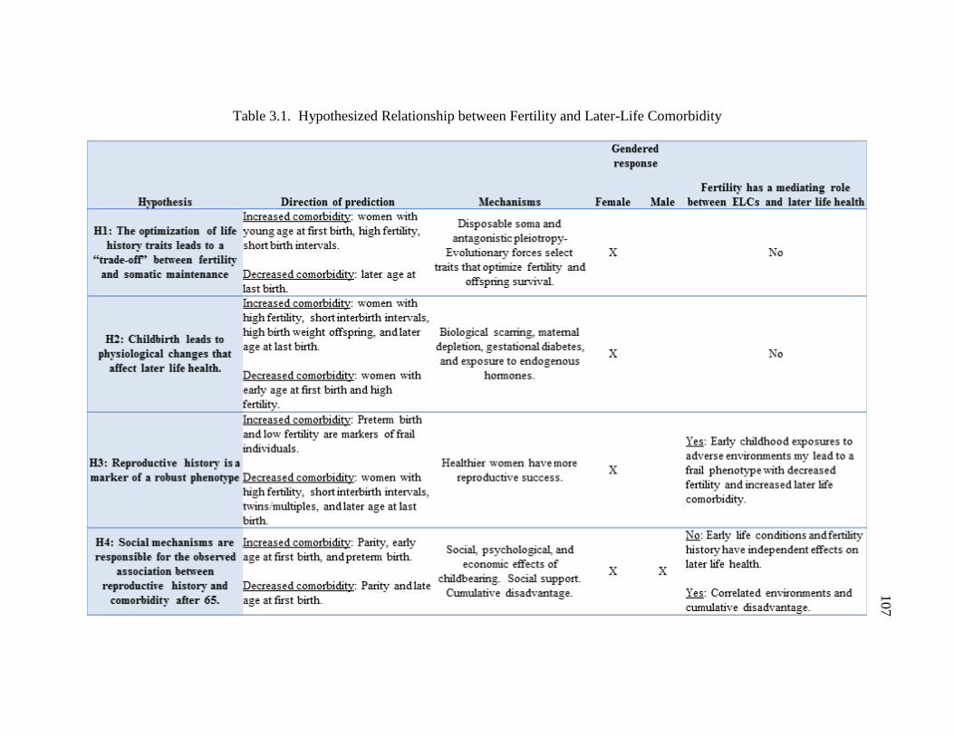
Table 3.1. Hypothesized Relationship between Fertility and Later-Life Comorbidity
107

108

109
Table 3.3. Descriptive Statistics by Gender and Age Group
Female 66-74 in
1992 Female 75 - 84
in 1992 Male 66-74 in
1992 Male 75 - 84 in
1992
N=12,190 N=10,099 N=11,349 N=7,520
Early Life Conditions N(% of total sample) or Mean (SD) Father's Nam-Powers SES Score 49.37 (19.54) 47.4 (18.19) 49.0 (19.14) 47.09 (17.96)
Father Farmer 3556 (29.2%) 3699 (36.6%) 3434 (30.3%) 2786 (37.1%) Father Missing SES 2982 (24.5%) 2416 (23.9%) 2620 (23.1%) 1754 (23.3%)
Active LDS 6452 (52.9%) 5525 (54.7%) 5876 (51.8%) 4219 (56.1%) InActive LDS 2886 (23.7%) 2883 (28.6%) 2643 (23.3%) 1843 (24.5%)
Non-LDS 2852 (23.4%) 1691 (16.7%) 2830 (24.9%) 1458 (19.4%) FEL Bottom 25% 2841 (23.3%) 2335 (23.1%) 2693 (23.7%) 1640 (21.8%) FEL Middle 50% 5321 (43.7%) 4525 (44.8%) 4869 (42.9%) 3648 (48.5%)
FEL Top 25% 2662 (21.8%) 2653 (26.3%) 2554 (22.5%) 1757 (23.4%) FEL Missing 1366 (11.2%) 586 (5.8%) 1233 (10.9%) 475 (6.3%)
Mother Died when Ego <18 721 (5.9%) 746 (7.4%) 682 (6.0%) 555 (7.4%) Mother Died when Ego 18+ 11379 (93.4%) 9255 (91.6%) 10583 (93.3%) 6906 (91.8%) Father Died when Ego <18 1060 (8.7%) 943 (9.3%) 951 (8.4%) 714 (9.5%) Father Died when Ego 18+ 11040 (90.6%) 9058 (89.7%) 10314 (90.9%) 6747 (89.7%)
Both Parents Died Before 18 90 (0.7%) 98 (1%) 84 (0.7%) 59 (0.8%) Fertility History
Children 1-2 3004 (24.6%) 3138 (31.1%) 2533 (22.3%) 2104 (28.0%) Children 3-5 6798 (55.8%) 5287 (52.4%) 6605 (58.2%) 4087 (54.4%) Children 6-8 2061 (16.9%) 1410 (14.0%) 1934 (17.0%) 1135 (15.1%) Children 9+ 327 (2.7%) 264 (2.6%) 277 (2.4%) 194 (2.6%)
Infant Death (Y/N) 730 (6.0%) 757 (7.5%) 637 (5.6%) 527 (7.0%) Short Birth Interval (Y/N) 3380 (27.7%) 2238 (22.2) 3489 (30.7%) 1707 (22.7%) Long Birth Interval (Y/N) 5201 (42.7%) 4684 (46.4%) 4568 (40.3%) 3513 (46.7%)
Mother/Father of Twin 580 (4.8%) 489 (4.8%) 486 (4.3%) 370 (4.9%) Age at First Bith Less than 18 391 (3.2%) 316 (3.1%) n/a n/a
Age at First Birth 18 - 24 8590 (70.5%) 5871 (58.1%) 5815 (51.2%) 2687 (35.7%) Age at First Birth 25+ 3209 (26.3%) 3912 (38.7%) 5534 (48.8%) 4833 (34.3%)
Age at Last Birth 35 - 39 1848 (15.2%) 3105 (30.8%) 2864 (25.2%) 2188 (29.1%) Age at Last Birth >=40 3827 (31.4%) 2369 (23.5%) 2864 (25.2%) 2995 (39.8%)
Age 70.09 (2.57) 79.00 (4.76) 70.0 (2.56) 78.6 (2.78) Information from Utah Birth Certificates*
At least 1 High Birth Weight Baby 668 (16.1%) 1126 (18.8%) At least 1 Low Birth Weight Baby 283 (6.8%)
434 (7.0%)
At Least One Preterm Birth 572 (13.8%)
942 (15.2%) Adult Measures
Spouse Alive at Baseline 9523 (78.1%) 5023 (49.7%) 10913 (96.2%) 6662 (88.6%) *Female N=4142; Male N=6192
Note: Age 66-74 in 1992 with birth certificate data on all births, making this a select
sample. Females are younger (avg age=69, range 66 - 74) and had to have their first birth
after age 20 (1947 is the first year BC available). Males are younger and had to have
their first birth after age 20.

110
Table 3.4. Sample Selection Means by Gender and Age
Mean (StdDev) Mean (StdDev)
Selection
Model
Female Age 66 - 74
Excluded
(N=48,519)
Included
(N=12,190) Probit P-value
Age in 1992 69.81(2.55) 70.09(70.09) 0.024 <0.001
Born in Utah 0.39(0.49) 0.85(0.85) 1.186 <0.001
1990 County Med Family Income
(Unit=10,000) 3.35(0.53) 3.28(3.28) -0.085 <0.001
1990 County Population (Unit=100,000) 5.87(12.4) 3.63(3.63) -0.018 <0.001
Missing 1990 Census Info 1% 0.30% -0.444 <0.001
Constant
-2.911 <0.001
Female Age 75 - 84
Excluded
(N=34,225)
Included
(N=10,099) Probit P-value
Age in 1992 78.95(2.79) 79(2.84) 0.01 0.01
Born in Utah 0.41(0.49) 0.83(0.38) 1.10 <0.001
1990 County Med Family Income
(Unit=10,000) 3.33(0.55) 3.26(0.42) -0.12 <0.001
1990 County Population (Unit=100,000) 6.07(13.26) 3.65(6.34) -0.01 <0.001
Missing 1990 Census Info 1% 0.10% -0.81 <0.001
Constant
-1.48 <0.001
Male Age 66 - 74
Excluded
(N=48,866)
Included
(N=11,349) Probit P-value
Age in 1992 69.79(2.56) 69.97(2.56) 0.02 <0.001
Born in Utah 0.4(0.49) 0.86(0.34) 1.24 <0.001
1990 County Med Family Income
(Unit=10,000) 3.34(0.57) 3.28(0.43) -0.10 <0.001
1990 County Population (Unit=100,000) 6.09(13.52) 3.77(6.56) 0.00 <0.001
Missing 1990 Census Info 1% 0.30% -0.55 <0.001
Constant
-2.61 <0.001
Male Age 75 - 84
Excluded
(N=29,211) Included (N=7,520) Probit P-value
Age in 1992 78.67(2.75) 78.63(2.78) 0.00 0.61
Born in Utah 0.4(0.49) 0.84(0.37) 1.16 <0.001
1990 County Med Family Income
(Unit=10,000) 3.28(0.57) 3.26(0.43) -0.08 <0.001
1990 County Population (Unit=100,000) 5.63(13.1) 3.71(7.08) -0.01 <0.001
Missing 1990 Census Info 1% 0.30% -0.59 <0.001
Constant -1.08 <0.001

111
Table 3.5. Effects of Early Life Conditions and Fertility on Comorbidity Trajectory
Group Membership versus Robust Group (19.1%): Women Ages 66 – 74 in 1992
Slow Initiates
Accelerated
Initiates Chronic Low Ailing Frail
18.8% 13.3% 19.7% 21.8% 7.3%
Early Life Conditions Odd Ratio (95% CI)
Age in 1992 2.47(1.88,3.26) 2.54(1.89,3.41) 3.52(2.71,4.58) 3.01(2.34,3.87) 3.16(2.24,4.45)
Active Member of LDS Church 0.76(0.61,0.94) 0.55(0.44,0.68) 0.72(0.58,0.88) 0.45(0.37,0.54) 0.47(0.37,0.61)
Inactive Member of LDS
Church 0.84(0.66,1.06) 0.57(0.45,0.73) 0.78(0.62,0.98) 0.59(0.48,0.73) 0.56(0.42,0.73)
Non-Member (reference) 1 1 1 1 1
Father's NP SES (unit=10) 1.02(0.98,1.05) 0.98(0.94,1.02) 1.01(0.97,1.04) 0.99(0.96,1.03) 0.96(0.91,1)
Father Farmer 1.01(0.85,1.2) 0.8(0.67,0.96) 1.1(0.93,1.29) 0.79(0.68,0.92) 0.74(0.6,0.93)
Missing SES 0.91(0.76,1.09) 0.91(0.76,1.1) 1.08(0.91,1.28) 0.85(0.73,1.01) 1.08(0.87,1.34)
FEL in Bottom Quartile 1.19(0.99,1.44) 1.38(1.14,1.67) 1.24(1.04,1.48) 1.44(1.22,1.69) 1.27(1.02,1.59)
FEL in Mid 50% (reference) 1 1 1 1 1
FEL in Top Quartile 0.79(0.67,0.94) 0.75(0.62,0.91) 0.71(0.61,0.84) 0.58(0.49,0.68) 0.7(0.56,0.87)
FEL Missing 0.97(0.74,1.27) 0.75(0.57,1) 0.84(0.64,1.09) 0.56(0.44,0.72) 0.45(0.32,0.63)
Orphaned before Age 18 2.39(0.91,6.29) 1.78(0.62,5.14) 1.46(0.53,4.05) 2.62(1.08,6.36) 3.87(1.44,10.4)
Mother Died before Child 18 1.1(0.82,1.49) 1.28(0.94,1.73) 1.11(0.83,1.48) 1.24(0.95,1.63) 1.48(1.05,2.1)
Father Died before Child 18 1.12(0.87,1.45) 1.38(1.07,1.78) 1.12(0.88,1.43) 1.24(0.99,1.56) 1.32(0.98,1.78)
Both Parents Alive at 18
(reference) 1 1 1 1 1
Fertility
1-2 Children 0.87(0.72,1.06) 1.07(0.88,1.31) 0.89(0.74,1.06) 0.95(0.8,1.13) 1.13(0.9,1.42)
3-5 Children (reference) 1 1 1 1 1
6-8 Children 1.09(0.87,1.35) 1.04(0.82,1.31) 1.1(0.9,1.36) 1.16(0.95,1.42) 1.1(0.83,1.45)
9+ Children 0.86(0.52,1.43) 1.06(0.65,1.74) 1.01(0.65,1.58) 1.2(0.79,1.84) 0.96(0.51,1.77)
Age at First Birth < 18 1.48(0.97,2.25) 1.48(0.96,2.3) 1.33(0.88,2.01) 1.44(0.98,2.12) 1.94(1.2,3.13)
Age at First Birth 18 - 24 (ref) 1 1 1 1 1
Age at first Birth >= 25 1.04(0.88,1.24) 0.86(0.71,1.03) 0.93(0.79,1.1) 0.86(0.74,1.02) 1.06(0.86,1.31)
Age at Last Birth 35 - 39 0.85(0.71,1.02) 0.83(0.68,1.01) 0.81(0.68,0.97) 0.82(0.69,0.97) 0.76(0.61,0.96)
Age at Last Birth >= 40 0.65(0.5,0.84) 0.8(0.61,1.05) 0.82(0.65,1.04) 0.66(0.52,0.83) 0.75(0.54,1.03)
Mother of Twins 1.17(0.84,1.62) 0.95(0.66,1.38) 0.96(0.69,1.32) 1.12(0.83,1.51) 1.01(0.67,1.54)
One or More Short Birth
Intervals 1.01(0.85,1.19) 1.11(0.93,1.33) 0.92(0.78,1.08) 1.03(0.88,1.21) 1.06(0.85,1.31)
One or More Long Birth
Intervals 1.01(0.87,1.19) 1.06(0.9,1.26) 0.93(0.8,1.09) 1.02(0.88,1.17) 0.97(0.79,1.19)
One or More Infant Deaths 0.93(0.69,1.24) 0.67(0.47,0.95) 0.83(0.62,1.1) 1.02(0.79,1.32) 1.13(0.8,1.6)
Sample Selection Bias IMR 1.13(0.92,1.39) 1.03(0.82,1.28) 1.06(0.86,1.29) 1.17(0.96,1.41) 1.3(1.02,1.67)
Note: Results shown in Table 3.5 are controlling for widowhood and jointly modeled
with mortality trajectories.

112
Table 3.6. Effects of Early Life Conditions and Fertility on Comorbidity Trajectory
Group Membership versus Robust Group (18.2%): Women Ages 75 – 84 in 1992
Initiates Chronic Low Ailing Frail
21.6% 29.7% 16.9% 13.6%
Early Life Conditions Odd Ratio (95% CI)
Age in 1992 1.84(1.38,2.44) 3.89(2.89,5.24) 2.77(2.16,3.55) 2.95(2.21,3.95)
Active Member of LDS Church 1.05(0.82,1.33) 0.83(0.65,1.07) 0.89(0.72,1.1) 0.93(0.72,1.19)
Inactive Member of LDS Church 1.12(0.87,1.45) 0.79(0.6,1.03) 0.97(0.78,1.22) 1.05(0.81,1.37)
Non-Member (reference) 1 1 1 1
Father's NP SES (unit=10) 1.02(0.98,1.07) 1.02(0.98,1.07) 1.02(0.98,1.06) 1(0.95,1.04)
Father Farmer 0.93(0.78,1.12) 1.07(0.87,1.31) 1.14(0.96,1.34) 0.93(0.77,1.13)
Missing SES 1.01(0.82,1.23) 1.07(0.86,1.34) 1.11(0.92,1.33) 1.08(0.87,1.34)
FEL in Bottom Quartile 1.44(1.17,1.77) 1.41(1.12,1.76) 1.59(1.33,1.91) 1.6(1.3,1.97)
FEL in Mid 50% (reference) 1 1 1 1
FEL in Top Quartile 0.77(0.64,0.91) 0.83(0.69,1.01) 0.65(0.56,0.77) 0.61(0.51,0.75)
FEL Missing 0.91(0.63,1.3) 1.11(0.77,1.6) 0.81(0.58,1.11) 0.78(0.53,1.14)
Orphaned before Age 18 0.88(0.42,1.85) 0.97(0.42,2.23) 1.29(0.68,2.43) 0.78(0.32,1.91)
Mother Died before Child 18 1.16(0.86,1.56) 1.31(0.96,1.78) 0.99(0.75,1.3) 1.35(1,1.81)
Father Died before Child 18 1.19(0.91,1.57) 1.15(0.86,1.54) 1.27(1,1.61) 1.24(0.94,1.63)
Both Parents Alive at 18 (reference) 1 1 1 1
Fertility
1-2 Children 0.98(0.8,1.21) 0.96(0.77,1.2) 0.9(0.75,1.08) 0.89(0.72,1.11)
3-5 Children (reference) 1 1 1 1
6-8 Children 1.01(0.79,1.31) 0.93(0.7,1.23) 1.22(0.97,1.53) 1.15(0.88,1.52)
9+ Children 0.77(0.43,1.38) 0.68(0.36,1.29) 1.17(0.73,1.89) 1.98(1.18,3.32)
Age at First Birth < 18 1.45(0.84,2.49) 1.85(1.05,3.24) 1.97(1.24,3.13) 2.03(1.23,3.36)
Age at First Birth 18 - 24 (ref) 1 1 1 1
Age at first Birth >= 25 0.86(0.72,1.03) 0.77(0.63,0.94) 0.9(0.77,1.06) 0.78(0.64,0.95)
Age at Last Birth 35 - 39 1.07(0.87,1.31) 1.38(1.11,1.72) 1.01(0.84,1.21) 1.11(0.9,1.37)
Age at Last Birth >= 40 1.13(0.89,1.45) 1.34(1.03,1.75) 0.89(0.71,1.11) 0.76(0.58,0.99)
Mother of Twins 1.08(0.76,1.54) 0.96(0.64,1.44) 1.02(0.74,1.4) 1.19(0.83,1.71)
One or More Short Birth Intervals 1.04(0.85,1.26) 0.83(0.66,1.04) 1.03(0.87,1.23) 0.89(0.72,1.1)
One or More Long Birth Intervals 0.76(0.63,0.91) 0.66(0.54,0.8) 0.82(0.7,0.96) 0.73(0.61,0.88)
One or More Infant Deaths 0.78(0.57,1.06) 0.84(0.6,1.17) 1(0.78,1.29) 1.07(0.8,1.44)
Sample Selection Bias IMR 0.95(0.75,1.21) 1.13(0.87,1.45) 1.12(0.9,1.39) 1.12(0.87,1.44)
Note: Results shown in Table 3.6 are controlling for widowhood and jointly modeled
with mortality trajectories.

113
Table 3.7. Effects of Early Life Conditions and Fertility on Comorbidity Trajectory
Group Membership versus Robust Group (15.7%): Men Ages 66 – 74 in 1992
Slow Initiates
Accelerated
Initiates Chronic Low Ailing Frail
16.4% 15.3% 18.5% 26.1% 8%
Early Life Conditions Odd Ratio (95% CI)
Age in 1992 1.4(1.01,1.94) 1.64(1.2,2.23) 2.33(1.73,3.15) 3.14(2.39,4.12) 3.41(2.36,4.91)
Active Member of LDS Church 0.76(0.59,0.98) 0.55(0.44,0.7) 0.82(0.65,1.03) 0.48(0.39,0.59) 0.4(0.31,0.52)
Inactive Member of LDS Church 0.66(0.5,0.86) 0.7(0.55,0.91) 0.75(0.58,0.97) 0.59(0.47,0.74) 0.45(0.34,0.6)
Non-Member (reference) 1 1 1 1 1
Father's NP SES (unit=10) 0.98(0.94,1.02) 1.01(0.97,1.05) 0.99(0.95,1.03) 1.02(0.98,1.05) 1.02(0.97,1.07)
Father Farmer 0.99(0.81,1.2) 1.05(0.87,1.27) 0.9(0.75,1.07) 1.13(0.96,1.33) 1.06(0.84,1.32)
Missing SES 1.05(0.85,1.3) 1.1(0.9,1.35) 0.96(0.79,1.18) 1.05(0.88,1.26) 1.14(0.9,1.44)
FEL in Bottom Quartile 1.2(0.96,1.49) 1.19(0.97,1.47) 1.28(1.05,1.57) 1.37(1.14,1.64) 1.3(1.03,1.65)
FEL in Mid 50% (reference) 1 1 1 1 1
FEL in Top Quartile 0.73(0.6,0.88) 0.71(0.59,0.86) 0.68(0.57,0.82) 0.66(0.56,0.78) 0.6(0.48,0.76)
FEL Missing 0.86(0.63,1.17) 0.88(0.65,1.18) 0.87(0.65,1.17) 0.55(0.42,0.72) 0.5(0.35,0.71)
Orphaned before Age 18 0.27(0.09,0.79) 0.57(0.24,1.34) 0.58(0.25,1.35) 0.72(0.37,1.41) 0.73(0.29,1.84)
Mother Died before Child 18 1.21(0.86,1.7) 1.18(0.85,1.64) 1.14(0.82,1.58) 1.21(0.9,1.62) 1.12(0.76,1.65)
Father Died before Child 18 1.14(0.85,1.54) 1.17(0.88,1.55) 1.08(0.82,1.43) 1.25(0.97,1.6) 1.07(0.77,1.5)
Both Parents Alive at 18
(reference) 1 1 1 1 1
Fertility
1-2 Children 1.04(0.82,1.3) 1.17(0.94,1.46) 1.14(0.92,1.41) 1.01(0.83,1.23) 1.25(0.96,1.61)
3-5 Children (reference) 1 1 1 1 1
6-8 Children 0.84(0.65,1.08) 1.04(0.82,1.32) 0.91(0.72,1.15) 0.91(0.74,1.13) 1.19(0.9,1.58)
9+ Children 0.63(0.37,1.08) 0.87(0.53,1.42) 0.63(0.37,1.05) 0.71(0.45,1.1) 0.77(0.41,1.47)
Age at First Birth <25 (ref) 1 1 1 1 1
Age at first Birth >= 25 0.88(0.74,1.05) 0.79(0.66,0.93) 0.78(0.66,0.92) 0.74(0.63,0.86) 0.78(0.63,0.95)
Age at Last Birth 35 - 39 0.99(0.8,1.23) 1.15(0.93,1.42) 0.98(0.8,1.2) 1.02(0.85,1.22) 1.12(0.88,1.43)
Age at Last Birth >= 40 1.04(0.79,1.37) 1.21(0.93,1.57) 0.88(0.68,1.14) 1.09(0.87,1.38) 0.94(0.69,1.29)
Father of Twins 0.94(0.64,1.4) 0.95(0.65,1.39) 1.2(0.85,1.71) 1.01(0.72,1.4) 1.13(0.73,1.75)
One or More Short Birth
Intervals 1.11(0.92,1.33) 0.94(0.78,1.13) 1.17(0.98,1.4) 1.01(0.86,1.18) 1.13(0.91,1.41)
One or More Long Birth
Intervals 1.08(0.9,1.29) 0.98(0.82,1.17) 1.17(0.98,1.39) 0.97(0.83,1.13) 1.06(0.86,1.31)
One or More Infant Deaths 0.83(0.59,1.18) 1.07(0.78,1.47) 0.83(0.6,1.14) 0.85(0.64,1.14) 0.85(0.57,1.25)
Sample Selection Bias IMR 0.89(0.7,1.14) 0.9(0.71,1.13) 0.91(0.73,1.13) 1.06(0.87,1.29) 0.98(0.75,1.28)
Note: Results shown in Table 3.7 are controlling for widowhood and jointly modeled
with mortality trajectories.

114
Table 3.8. Effects of Early Life Conditions and Fertility on Comorbidity Trajectory
Group Membership versus Robust Group (14.7%): Men Ages 75 – 84 in 1992
Initiates Ailing Chronic Low Frail
17.4% 35.3% 20.2% 12.5%
Early Life Conditions Odd Ratio (95% CI)
Age in 1992 1.6(1.09,2.34) 2.24(1.65,3.05) 2.12(1.5,3) 2.82(1.94,4.1)
Active Member of LDS Church 0.81(0.6,1.07) 0.78(0.62,1) 0.8(0.61,1.05) 0.72(0.53,0.96)
Inactive Member of LDS Church 1.01(0.73,1.4) 0.98(0.75,1.28) 0.97(0.71,1.31) 0.97(0.7,1.34)
Non-Member (reference) 1 1 1 1
Father's NP SES (unit=10) 1(0.94,1.06) 1(0.95,1.04) 1.01(0.95,1.06) 0.96(0.9,1.02)
Father Farmer 0.95(0.75,1.21) 0.94(0.77,1.14) 0.95(0.76,1.19) 1.09(0.85,1.38)
Missing SES 1.06(0.81,1.38) 0.85(0.68,1.06) 0.9(0.7,1.16) 0.98(0.74,1.29)
FEL in Bottom Quartile 1.38(1.06,1.81) 1.7(1.36,2.13) 1.28(0.99,1.66) 1.89(1.46,2.46)
FEL in Mid 50% (reference) 1 1 1 1
FEL in Top Quartile 0.8(0.63,1.01) 0.77(0.64,0.94) 0.91(0.73,1.14) 0.67(0.52,0.87)
FEL Missing 0.71(0.45,1.11) 0.76(0.53,1.1) 0.99(0.66,1.49) 0.84(0.53,1.33)
Orphaned before Age 18 1.16(0.34,3.94) 1.28(0.5,3.24) 0.67(0.18,2.45) 0.43(0.1,1.84)
Mother Died before Child 18 1.14(0.78,1.68) 1.36(0.99,1.87) 1.11(0.77,1.61) 1(0.66,1.51)
Father Died before Child 18 1.01(0.73,1.39) 0.97(0.75,1.27) 0.79(0.57,1.09) 1(0.72,1.39)
Both Parents Alive at 18 (reference) 1 1 1 1
Fertility
1-2 Children 1.01(0.76,1.34) 0.95(0.75,1.2) 1.07(0.82,1.39) 0.97(0.73,1.29)
3-5 Children (reference) 1 1 1 1
6-8 Children 0.81(0.59,1.12) 1.14(0.88,1.47) 0.89(0.66,1.19) 0.77(0.55,1.07)
9+ Children 0.82(0.43,1.57) 0.81(0.47,1.4) 0.76(0.41,1.4) 0.61(0.31,1.2)
Age at First Birth <25 (ref) 1 1 1 1
Age at first Birth >= 25 0.97(0.77,1.23) 0.82(0.68,1) 0.86(0.69,1.07) 0.71(0.56,0.9)
Age at Last Birth 35 - 39 0.96(0.72,1.28) 0.85(0.67,1.08) 0.79(0.6,1.04) 0.73(0.54,0.98)
Age at Last Birth >= 40 0.94(0.67,1.31) 0.74(0.56,0.97) 0.94(0.69,1.28) 0.81(0.58,1.12)
Father of Twins 0.86(0.54,1.37) 0.71(0.48,1.05) 1.25(0.84,1.86) 1.12(0.71,1.74)
One or More Short Birth Intervals 1.16(0.9,1.51) 0.92(0.74,1.14) 0.98(0.76,1.25) 1.15(0.88,1.49)
One or More Long Birth Intervals 1.11(0.88,1.39) 1.05(0.87,1.26) 1.12(0.9,1.38) 1.1(0.87,1.39)
One or More Infant Deaths 1.03(0.69,1.55) 1.27(0.92,1.76) 1.01(0.69,1.49) 0.96(0.64,1.46)
Sample Selection Bias IMR 1.21(0.89,1.64) 1.38(1.07,1.78) 1.15(0.86,1.54) 0.98(0.71,1.36)
Note: Results shown in Table 3.8 are controlling for widowhood and jointly modeled
with mortality trajectories.

115
Figure 3.1. Comorbidity trajectories for females ages 66 – 74 in 1992.
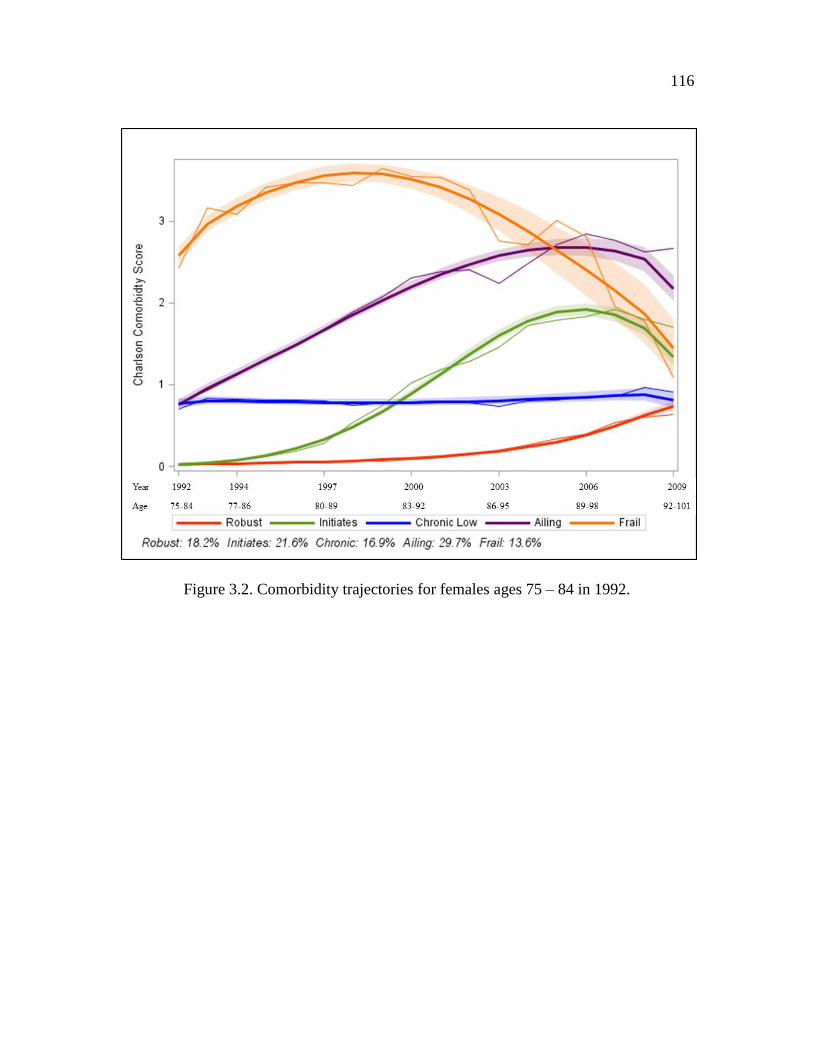
116
Figure 3.2. Comorbidity trajectories for females ages 75 – 84 in 1992.

117
Figure 3.3. Comorbidity trajectories for males ages 66 – 74 in 1992.
** **

118
Figure 3.4. Comorbidity trajectories for males ages 75 – 84 in 1992.

119
Figure 3.5. Morbidity trajectories for females ages 66 – 74 in 1992.

120
Figure 3.6. Morbidity trajectories for females ages 75 – 84 in 1992.

121
Figure 3.7. Morbidity trajectories for males ages 66 – 74 in 1992.

122
Figure 3.8. Morbidity trajectories for males ages 75 – 84 in 1992.

123
Figure 3.9. Female birth certificate results: Ages 66 – 74 in 1992. Controlling for early-
life conditions, fertility variables, demographic characteristics, and jointly modeled with
mortality trajectories. Birth certificate sample (N=4,214)
0.00
0.50
1.00
1.50
2.00
2.50
HB
W O
ffsp
rin
g
LBW
Off
spri
ng
Pre
term
Off
spri
ng
HB
W O
ffsp
rin
g
LBW
Off
spri
ng
Pre
term
Off
spri
ng
HB
W O
ffsp
rin
g
LBW
Off
spri
ng
Pre
term
Off
spri
ng
HB
W O
ffsp
rin
g
LBW
Off
spri
ng
Pre
term
Off
spri
ng
HB
W O
ffsp
rin
g
LBW
Off
spri
ng
Pre
term
Off
spri
ng
Slow Initiates(19.2%)
AcceleratedInitiates (14.3%)
Chronic Low(18.0%)
Ailing (21.3%) Frail (6.9%)
Od
ds
Rat
io
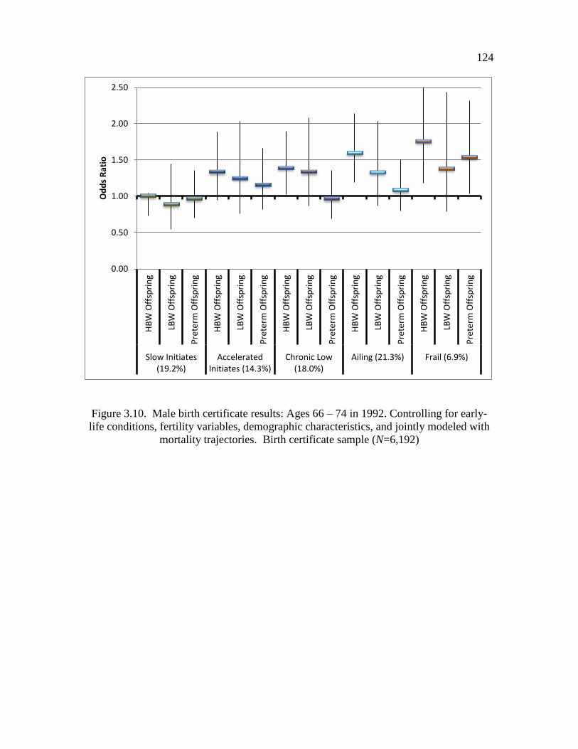
124
Figure 3.10. Male birth certificate results: Ages 66 – 74 in 1992. Controlling for early-
life conditions, fertility variables, demographic characteristics, and jointly modeled with
mortality trajectories. Birth certificate sample (N=6,192)
0.00
0.50
1.00
1.50
2.00
2.50
HB
W O
ffsp
rin
g
LBW
Off
spri
ng
Pre
term
Off
spri
ng
HB
W O
ffsp
rin
g
LBW
Off
spri
ng
Pre
term
Off
spri
ng
HB
W O
ffsp
rin
g
LBW
Off
spri
ng
Pre
term
Off
spri
ng
HB
W O
ffsp
rin
g
LBW
Off
spri
ng
Pre
term
Off
spri
ng
HB
W O
ffsp
rin
g
LBW
Off
spri
ng
Pre
term
Off
spri
ng
Slow Initiates(19.2%)
AcceleratedInitiates (14.3%)
Chronic Low(18.0%)
Ailing (21.3%) Frail (6.9%)
Od
ds
Rat
io
CHAPTER 4
HERITABILITY OF LONGEVITY AND THE ROLE OF EARLY
AND MIDLIFE ENVIRONMENTS3
Introduction
Mortality is the quintessential measure of the health of a population, and large
gains in human life expectancy over the past 150 years are evidence of the important
relationship between social context and health. While there is certainly variability in
longevity between populations, there is also wide variation in longevity within
populations. Understanding the determinants of this heterogeneity is essential to
understanding the processes of aging and health of a population. But how much of this
variation is determined by genetic factors and how much is determined by the
environment? While the question of heritability of longevity is not new, with heritability
estimates of longevity ranging from 0 to 0.3 (Kerber, O'Brien, Smith, & Cawthon, 2001),
we seek to determine if heritability estimates vary between subpopulations and explore
the possibility of gene-environment interactions (GxE). By examining sources of
3 Coauthored by Ken R. Smith and Sandra Hasstedt. We wish to thank the Pedigree and
Population Resource of the Huntsman Cancer Institute, University of Utah for providing
the data and valuable computing support. This work was also supported by NIH grant
AG022095 (Early-life Conditions, Survival and Health; Smith PI).
126
variation in heritability estimates, we can illuminate factors that modify the expression of
genetic predisposition in a population.
We will investigate heterogeneity in the genetic basis of longevity by assessing
the phenotypic correlation between relatives. Variance components and heritability
values will be generated using a large genealogical database with information on family
structure as well as measures of the broader environment. This study will examine the
relationship between social context and the amount of additive genetic variance in adult
life-span and exceptional longevity using data from the Utah Population Database
(UPDB), a rich source of linked population-based information for demographic, genetic,
and epidemiological studies. The sample used in this study consists of 20,120 individuals
from 802 three generation pedigrees. This analysis has two goals: 1) estimate the
heritability of longevity after age 30 as well as exceptional longevity in a population
using methods designed for use in multigenerational pedigree information; 2) test for
differences in heritability estimates of life-span in populations stratified by environmental
exposure.
Background
Heritability of Longevity
Over the past few decades, demographers have broadened the focus of work in the
demography of aging from a population aging perspective (i.e., measures of change in
population age structure) to include a perspective that integrates health and biological
explanations with traditional demographic and social theories of aging to explain
heterogeneity in health and mortality within and between populations (Olshansky,
Carnes, & Brody, 2002; Siegel, 2011; Vasunilashorn & Crimmins, 2008). While it is

127
widely accepted that life-span is determined by a combination of genetic, social and
physical environment, and stochastic factors, the interdependent and dynamic role of
genes and environment is still not well understood. This may be partially due to fears of
genetic determinism within the field of sociology (Shostak & Freese, 2010), the divergent
paths of genetics and demography (Adams, 1990), and the difficulty of assessing the role
of genes and environment biomarker data.
Longevity is a complex trait, determined by a multiplicity of genetic and
environmental factors, each of which contributes to a potentially small amount of
phenotypic variation. The genetic variation that is the natural background is a shortened
life-span (relative to exceptional longevity) and exceptional longevity is the result of
mutations. Genes affecting longevity have been parsed into two categories described as
gerontogenes: genes that have a negative effect on longevity and longevity-assurance
genes that promote longevity (Christensen, Johnson, & Vaupel, 2006). Findings from the
New England Centenarian Study (NECS) have suggested that supercentenarians do not
lack gerontogenes, but have longevity assurance genes that can counter the deleterious
effects of genes and environment as well as slow the rate of aging and lead to delayed
onset of age-related disease (Sebastiani et al., 2012). It is also believed that longevity
mutations increase the ability to handle stress and robustness (Christensen et al., 2006).
The proportion of variation in life-span due to genes is moderate, which can be illustrated
by the fact that there is variation in life-span between monozygotic twins (Herskind et al.,
1996).
In summary, longevity is determined by a complex relationship between both
genes and environment. For a more complete understanding of population heterogeneity
in life-span and the forces behind it, one must not only understand the average

128
contribution of genes and environment within a population toward explaining variation in
adult mortality, but uncover the factors that influence patterns of variation within the
population.
At the most basic level, phenotypic variation can be partitioned into additive
genetic variance and general environmental variance. Additive genetic variance is the
deviation from the average phenotype that is due to the inheritance of a particular allele
and that allele’s effect on the phenotype. General environmental variance can then be
described as the remaining variance that cannot be attributed to genes. The proportion of
variation due to inheritance of a particular allele is not fixed across all environments
because the relationship between genotype and phenotype may vary by environment, a
phenomenon known as phenotypic plasticity. Narrow sense heritability is a population
level statistic that describes the amount of total phenotypic variation (VT) that can be
attributed to additive genetic variation (VA) in the population (h2
= VA/VT). The
polygenic model can be used to partition variation into genetic and residual
environmental effects. Because it is a population level statistic, it is important to keep in
mind that it not a property of individual traits. When h2equals zero, it indicates that all
phenotypic variation within a population can be explained by individual differences,
while an h2
of 1 indicates that all the phenotypic variation is explained by genetic
differences. This is not to say that high heritability suggests little environmental effect on
the phenotype. When h2 is elevated the environment may uniformly contribute to the
expression of the trait and therefore contribute little to differences between people. It has
been shown that heritability of traits can vary across subpopulations (Boardman, 2009;
Boardman et al., 2012; Rowe, Almeida, & Jacobson, 1999). But how much of the
population heterogeneity in life-span is determined by genetic factors?

129
There is evidence of the presence of familial clustering of longevity over many
generations and across diverse populations, suggesting that there is a genetic or familial
component to successful aging and longevity (Christensen et al., 2006; Finch & Tanzi,
1997; Herskind et al., 1996; Kerber et al., 2001; Perls, Kunkel, & Puca, 2002). The
longevity literature has described the genetic and environmental contribution to mortality
as being divided into one-third and two-third proportions, respectively (C. E. Finch &
Tanzi, 1997; Siegel, 2011). It has also been suggested that 50% of the variation in life-
span after age 30 can be ascribed to attributes (genetic and nongenetic) that are fixed
prior to that age (Yashin & Iachine, 1997), and that genetics plays a stronger role with
advancing age (Hjelmborg et al., 2006; Montesanto, Dato, Bellizzi, Rose, & Passarino,
2012; Vaupel et al., 1998; see J. W. Rowe and Kahn (1997) for a dissent from this view).
If the proportion of variation in life-span that can be explained by genetic factors varies
by age, is it also conditioned by social context? And if so, does this conditioning vary by
age?
Conceptualizing the Relationship between Social Environment
and Heritability of Longevity
Attempting to understand the genetic component of longevity without considering
how it may be modified by specific environmental factors may not be a fruitful approach
to gaining insights into the heritability of this complex trait (Petronis, 2010). The
heritability of certain phenotypes may vary throughout the life course (Turkheimer,
Haley, Waldron, D'Onofrio, & Gottesman, 2003) and by gender (Visscher, Hill, & Wray,
2008). Given that humans are constantly interacting with the environment and the
environment has the ability to alter gene expression, we must also understand how

130
environmental influences might modify the heritability of longevity. Accordingly, in this
analysis, comparisons of heritability will be made between three subgroups of the
population based on: 1) religious involvement; 2) early disease and nutritional
environment; and 3) family environment during childhood.
This study assumes that the same genes affect longevity across environments
within a population, but certain attributes of the environment serve to moderate the effect
of genes on phenotypic variation. Shanahan and Hofer (2005) have presented a
framework for gene and social context interactions that has been used to explain the
relationship between the social environment and health behaviors (Boardman, 2009;
Boardman et al., 2012). We present a slightly modified version that also utilizes concepts
presented by Hoffmann and Merilä (1999) as well as new modifications to help formulate
our hypotheses.
Under Shanahan and Hofer’s framework for gene-environment (GxE)
interactions, the environment is conceptualized as social context (Shanahan & Hofer,
2005). Four perspectives, described in detail below, can be used to depict how the social
environment might affect heritable variation: triggering, compensation, social control,
and enhancement. Figures 4.1 – 4.4 show a modified version of a schema presented by
Sebastiani et al. (2012) describing the genetic components of aging. Sebastiani et al.
have hypothesized that individuals living to exceptional ages have gerontogenes, but the
longevity assurance genes counter the deleterious effects of genetic and environmental
factors. Figure 4.1 shows the proportion of total phenotypic variance (VT) that is
attributable to additive genetic variance (VA) and environmental variance (VE), where the
phenotype is longevity after age 30. We show that in a normal environment where there
is no GxE interaction (panel A), individuals with shorter life-spans have higher

131
heritability of gerontogenes and individuals with exceptional life-spans have higher
heritability of longevity assurance genes.
A triggering effect refers to an environment that interacts with personal
predispositions to a diseased state and shortened life-span through, for example,
environmental stressors or other factors that induce a biological change. Figure 4.2
shows the hypothesized triggering GxE interaction in which an adverse environment
directly affects the phenotype. When triggering mechanisms are responsible for
environmental differences in heritability, we expect to see a decrease in average
longevity in adverse environments and an increase in additive genetic variance. This is
because the environment leads to phenotypic expression that would otherwise be
dormant. This relationship may change with exceptional longevity because selection
mechanisms may change the heritability of a trait over time. If the genetically frail
individuals are selected out of this population at an earlier age, the surviving population
may be comprised of more robust individuals with a genetic predisposition for
exceptional longevity (i.e., longevity assurance genes; Hawkes, Smith, & Blevins, 2012),
leading to higher levels of heritability of exceptional longevity in environments
detrimental to health. Therefore, under this formulation, we expect that individuals
exposed to an unhealthy environment during childhood will have higher heritability of
longevity, but a shorter life-span compared to those living in more advantageous
circumstances. This may also translate into higher heritability of exceptional longevity in
unhealthy environments because only the robust in an unhealthy environment survive to
exceptional ages.
The second type of GxE interaction is compensation. According to this
perspective, in normal and adverse environments the predisposition to a diseased state

132
and shortened life-span is realized but not in enriched settings. The expected change in
additive genetic variance in an enriched environment is presented in Figure 4.3. The
compensation GxE perspective assumes that the continuous exposure to a healthy
environment prevents the expression of a genetic diathesis that predisposes an individual
to premature death. Unlike the triggering mechanism, the relationship between
environment and phenotype is not causal, but due to environmental variation. Therefore,
we would expect to see an increase in average life expectancy in an enriched environment
with lower additive genetic variance for the longevity phenotype.
Social control is the third GxE model. This interaction is not presented in Figures
4.1 – 4.4 because the expected outcomes are similar to those presented in Figure 4.3.
Heritability of longevity may be attenuated in environments with high social control
because social norms and structural constraints place limits on choices, and, therefore the
environment suppresses phenotypic variance. This is similar to the evolutionary
argument of canalization, which argues that selection favors suppression of quantitative
traits in constant and structured environments, but the genotype maintains a potential for
expressing certain phenotypes under particular environmental conditions (Hoffmann &
Merilä, 1999). Thus, involvement with a religious institution that maintains strong social
norms for health related behaviors such as alcohol consumption, smoking, social support,
and dietary restrictions may lead to increased longevity and exceptional longevity for all
members of the group and suppress genetic predispositions for disease. In this situation,
we expect to see increased longevity and exceptional longevity for active religious
participants with lower levels of heritability compared to nonparticipants.
The enhancement model of GxE is presented Figure 4.4. This is similar to the
social control mechanism, but rather than suppressing a predisposition to a shortened life-
133
span, social context can serve to enhance genetic predispositions for longevity.
Individuals in advantaged and organized social settings may be more apt to realize their
genetic potential for longevity, while disadvantaged environments lead to unrealized
potential. For example, an environment of undernutrition or high levels of exposure to
infectious agents may lead to physiological changes that alter an individual’s ability to
reach their genetic potential (Barker, 1995; Barker et al., 1993; Crimmins & Finch,
2006). Here, we would expect to see mean differences in survival between environments
and higher heritability of life-span and exceptional longevity in environments more
advantageous for health and longevity.
In this paper, we build on a body of literature that examines the heritability of
longevity by comparing heritability of longevity and exceptional longevity between sub-
populations exposed to different environments that are known to affect adult mortality
risks. Using the GxE perspectives discussed above, we compare the heterogeneity of
genetic effects by environment. We expect to see differences in the heritability of
longevity between environments characterized as salubrious or unhealthy. The GxE
categories of triggering, compensation, and social control predict higher levels of
heritability of longevity in environments less beneficial to health, while the enhancement
typology predicts increased heritability of longevity in healthy environments. We can
make generalizations about what type of GxE interaction leads to the observed patterns,
but the exact mechanism is not testable under this formulation. Comparing the
components of variance between environments will add to the understanding of the
relative importance of both genes and environment in determining longevity.

134
Methods
Data
The majority of life-span epidemiological studies examine health influences of
early and adult life conditions with relatively modest sample sizes, particularly given the
complexity of the phenomena and the manifold exposures and outcomes. This study
utilizes data drawn from the Utah Population Database (UPDB). The UPDB is one of the
world’s richest sources of linked population-based information for demographic, genetic,
and epidemiological studies. UPDB has supported biodemographic studies as well
numerous important epidemiological and genetic studies in large part because of its size,
pedigree complexity, and linkages to numerous data sources. In the mid-1970s, over
185,000 three-generation families were identified on Family Group Sheets from the
archives at the Utah Family History Library. These families have been linked into
multigenerational families and the full UPDB now contains data on nearly 7 million
individuals due to longstanding and on-going efforts to add new sources of data and
update records as they become available.
Mortality data are fundamental to the study of exceptional longevity. Information
on deaths prior to 1904 comes from genealogical records obtained from the Utah Family
History Library and linked to other records within the UPDB. All Utah death certificates
are available from 1904 to the present. The UPDB also links to the U.S. Social Security
Death Index (SSDI) for the years 1936 – 2011. The SSDI records provide information on
deaths based on Social Security records regardless of place of death and are linked to the
UPDB. The unique combination of genealogy, death certificates, and SSDI data provide
wide spatial and temporal coverage for both the fact and date of death.

135
The sample used to construct measures of longevity comprises all individuals in
the UPDB born between 1850 and 1927. We selected 1927 as the maximum birth year to
allow us to observe mortality to at least age 85 for the youngest members of the cohort.
To minimize variability in survival unrelated to aging and based on other evidence of the
fixed attributes related to life-span after age 30 (Yashin & Iachine, 1997), we will model
mortality beginning at age 30 (Hawkes et al., 2012). We identified 685,949 individuals
who met the criteria listed above. Of those, approximately 9% (n=64,258) were right
censored and 91% (N=621,961) had vital status follow-up information from family
history group sheets, Utah death certificates, or linked Social Security Death Index
(SSDI) information. The gender distribution of the sample was 52.5% male and 47.5%
female.
Using individuals from the baseline survival analysis, we selected 111,324 three-
generation families. Table 4.1 shows the restrictions imposed at the family level. We
attempted to select families with the highest data quality and the most complete
information. As a result, 31,322 families were excluded from the analysis because at least
one grandparent had no information in the UPDB. All founding pedigree members were
required to have a birth year greater than 1850 (Utah was settled in 1847) and all
members of the family were required to be born before 1928, which allowed us to
observe the youngest members of the cohort to age 84. On average, these families had 4
individuals in the first generation (by definition), 13 individuals in the second generation,
and 19 individuals in the third generation (range = 1 to 83). Pedigree size ranged from 7
to 109 members. The final sample consisted of 802 three-generation families with 20,120
members with a calculated longevity measure and information on family of origin. To
study exceptional longevity, a nearly deceased cohort is needed. Therefore, individuals

136
born between 1914 and 1927 were excluded from the exceptional longevity sample,
yielding a sample of 14,618 individuals for these analyses.
Measuring Early and Midlife Environments
Both early and midlife conditions will be considered as possible social context
that may modify phenotypic expression. To simplify both the measurement and
conceptualization of the environment, each environment is treated as a simple dichotomy,
comparing salubrious environments to those that are less advantageous to health. We
will compare the heritability of longevity by religious participation, infant mortality rate
(IMR) in the family of origin, childhood mortality rate (CMR) of the family of origin,
and number of siblings. Justifications for each as the basis for deleterious and beneficial
environments are described in turn below.
Religious involvement in general is associated with increased life expectancy
(Hummer, Rogers, Nam, & Ellison, 1999). It is not surprising that active affiliation with
the Church of Jesus Christ of Latter-day Saints (LDS or Mormon) church is also
associated with increased life expectancy (Enstrom & Breslow, 2008). Individuals
actively affiliated with the LDS church are more likely to abstain from alcohol and
tobacco use, fast once a month, and participate in church related social activities (Mineau,
Smith, & Bean, 2002). Therefore, affiliation with the LDS church will be treated as a
social environment with defined healthy lifestyle norms for men and women. The UPDB
contains information on baptism dates from family history records, which were used to
classify individuals as followers of the LDS church. Individuals baptized as members of
the LDS church before the age of 30 are considered followers of the LDS Church.

137
Individuals will be parsed into two environments: 1) LDS church involvement; and 2) no
LDS church involvement.
Early life health can have long-term consequences on later life health and
mortality (Elo & Preston, 1992; Smith, Mineau, Garibotti, & Kerber, 2009). While it is
difficult to obtain a measure of early life exposure to disease and other adverse
circumstances, we can use mortality outcomes of siblings as a sentinel for early life
circumstances. Postneonatal mortality (the first year of life excluding the first 28 days)
for our cohorts of study (1850 – 1927) is closely related to viral and bacterial disease,
malnutrition, and income (B. K. Finch, 2003; McKeown, 1976; Preston & Haines, 1991).
A similar argument has been made for childhood mortality by Crimmins and Finch
(2006), who argue that birth cohorts with lower childhood mortality have increased
longevity. As such, we use the death of a sibling during the first year of life (IMR in
family of origin) or between ages 1 and 5 (CMR in family of origin) as indicators of an
adverse childhood environment. Neonatal deaths, deaths within the first 28 days, and
stillbirths are not included in our final measure of IMR because these deaths are likely
due to endogenous causes and may not represent a family environment marked by
disease, an assumption most likely to be true for the years considered here. We consider
infant and childhood mortality as distinct environments because it has been suggested
that the determinants of infant and childhood mortality decline over time differed during
this period (Wolleswinkel-van den Bosch, van Poppel, Looman, & Mackenbach, 2000).
Individuals with one or more infant or childhood death in their family of origin (i.e.,
death of a sibling) were considered to be in an environment of high infant or childhood
mortality, respectively.

138
Sibship size (number of siblings) has been shown to be positively associated with
lower educational achievement and unhealthy lifestyle choices (Downey, 1995; Hart &
Davey Smith, 2003). Sibship size may also be related to exposure to infectious diseases,
with children from large sibships having a greater risk of contracting an infectious
disease (Hart & Davey Smith, 2003). However, a strong association between sibship size
and adult mortality has not been demonstrated in all studies assessing this relationship
(Smith et al., 2009). The definition of large sibship was derived empirically as having 7
or more siblings (75th
percentile for the sample).
While sex is inherently a biological trait, sex differences in life expectancy are
determined by both social and biological factors (Crimmins & Saito, 2001; Lindahl-
Jacobsen et al., 2013; Rieker, Bird, & Lang, 2010). The effects of early life conditions on
later life health may differ by sex. Male fetuses have higher mortality rates than female
fetuses, a disadvantage that continues throughout the life course (Kraemer, 2000). Earlier
studies have found slight differences in the heritability of longevity between males and
females, with males having higher heritability than females (Herskind et al., 1996).
Accordingly, we test for environmental differences in the heritability of longevity by sex.
Definition of Longevity
The mortality schedule for individuals born between 1850 and 1927 has changed
considerably. Longevity, therefore, defined simply as years lived after age 30, is not
appropriate because it is not directly comparable across birth cohorts. While much of the
improvement in life expectancy seen during this period was due to improvements in
infant and child mortality, there were also gains in adult mortality. Cohort life tables for
Utah show that individuals born in 1850 and surviving to age 30 could expect to live an

139
additional 40.5 and 39.5 years for females and males, respectively, compared to 53.1 and
48.5 years of additional life after 30 for individuals born in 1920 (Lindahl-Jacobsen et al.,
2013). Therefore, to de-trend the data, we define longevity as the difference between an
individual’s attained age (y) and the age to which that individual was expected to live
(median predicted age of death conditioned on surviving to 30, ̂) according to a model
that incorporates two basic determinants of life-span: gender and birth year. Therefore, a
longevity score (LS) is simply the difference between these two values, y - ̂. The
baseline survival models used to determine ̂ are described below. This approach is
similar to one taken by Kerber et al. (2001) in calculating a measure of familial excess
longevity using Utah genealogies.
Previous studies have suggested that the heritability of longevity increases with
age (Hjelmborg et al., 2006; Yashin & Iachine, 1997), and may perhaps be the strongest
for those surviving to the latest ages (Atzmon et al., 2004; Gudmundsson, Gudbjartsson,
Frigge, Gulcher, & Stefánsson, 2000; T. T. Perls, Bubrick, Wager, Vijg, & Kruglyak,
1998). Exceptional longevity can be defined as an exceptionally long life-span compared
to other individuals experiencing the same historical influences (birth cohort; Michael
Anson et al., 2012). As done in previous studies, we will define the exceptional
longevity (EL) phenotype as living to exceptional age, and explore differences in
heritability of survival to the 90th
and 95th
percentile based on the baseline hazard models
(Kerber, O'Brien, Boucher, Smith, & Cawthon, 2012).
Constructing Baseline Survival Models
We assume a parametric form for the survival distribution and a generalized class
of accelerated failure time (AFT) models, the extended family of generalized gamma

140
models. Unlike proportional hazard models, AFT models assume that the effect of
covariates is multiplicative with respect to survival time. We test the fit of the
exponential, Weibull , log-normal, log-logistic, and gamma models. These models were
selected because they provide a simple point estimate for duration that generally fits the
observed data for adult mortality. While the gompertz model is appropriate for modeling
human mortality between 30 and 85 (Olshansky & Carnes, 1997), this study is concerned
with exceptional longevity (past the age of 85) and therefore this model was not
considered. The nested structure of the family of generalized gamma models
(exponential, Weibull, log-logistic, and gamma) allows for use of the likelihood ratio test
to assess model fit. The Akaike information criterion, or AIC, can be used to test the fit
of nonnested models. Final models were selected for the construction of the longevity
measures based on model fit.
The full sample of 685,949 individuals born between 1850 and 1927 meeting the
sample criteria described in the data section above were used to estimate survival time for
individuals surviving to age 30. Models were stratified by gender and included two
covariates, birth year, and birth year squared. All models showed a significant positive
relationship between birth year and survival. The generalized gamma model proved to be
the best fit based on likelihood ratio test (p<0.001) and AIC. The shape and scale
parameters in the generalized gamma model are also significantly different than “0” and
“1,” implying that the fitted distribution is different from the Weibull, log-normal, and
exponential models. The change in the predicted 50th
and 90th
percentile by model and
year is displayed in Figure 4.5. Panels A and B show the trend in predicted median and
90th
percentile longevity respectively for men and panels C and D display the estimates
for women. The exponential model does not fit the data well and therefore the results are
141
not shown. These figures show that the log-normal and log-logistic models, which
provided the worst fit based on the AIC statistic, also predict out of range values for the
90th
percentile. Both the Weibull and generalized gamma model provide sensible
estimates. Therefore, the generalized gamma model was used to estimate ̂ and
consequently LS.
LS was defined as the observed, minus the expected, life-span for all deceased
individuals. The UPDB contains multiple sources of linked records that can be used to
create a last observed date. Therefore, we know that individuals without a death record
were alive until their last observed date in UPDB. The observed life-span for individuals
born after 1905, not deceased, and with a known follow-up date that exceeded the median
predicted survival time for their gender and birth cohort is calculated by subtracting the
birth year from the last observed date in UPBD. Therefore, censored individuals that are
likely still living were used in the LS analyses and have a positive LS score by definition.
To test for biased results created by this specification, we ran sensitivity analysis using
the nearly deceased cohort (N=14,618).
Heritability Estimates
Several forms of analysis of variance (ANOVA) are available to measure
heritability of a phenotypic trait, such as parent-offspring regressions and sibling
analyses. While these models have useful features, they are limited because they do not
use information from multigenerational relationships and they require that sample sizes
be well-balanced. Unlike other forms of analysis of variance (ANOVA), maximum
likelihood (ML) estimators do not place special demands on the design or balance of the
data, providing a powerful approach to estimating variance components using large
142
pedigrees (Lynch & Walsh, 1998) and minimizing the inflation of estimates of additive
genetic variance due to shared environments between relatives. To allow for use of
information on multigenerational relationships, heritability is estimated with a polygenic
model using PAP v. 7.1 (Hasstedt, 2005).
Genotypic variance can be decomposed into additive , dominance , and
epistatic . and are, however, extremely difficult to estimate in non-
experimental settings (Kruuk, 2004). The polygenic model specifies the expected genetic
relationship between relatives as a function of the coefficient of relationship, allowing for
the estimation of variation due to genetic and residual environmental effects. The
coefficient of relationship is (1/2)p, where p is the degree of relationships (it is also
commonly described as two times the probability that two individuals will share a
common gene by descent (IBD)). For example, for a parent-child relationship the
coefficient of relationship is 0.5, which equals 2 x 0.25, where 0.25 is the probability that
parent and child share a common allele. The polygenic model allows us to partition the
total phenotypic variance ( ) into the following components:
(eq. 4.1)
where is the additive genetic variance and
is the residual variance, which includes
environmental, dominance, and epistatic effects. These components are used to
calculate heritability, with narrow sense heritability (h2) being defined as the proportion
of phenotypic variance,
, that can be attributed to the additive genetic effects, :
h2=
/ (eq. 4.2)
The polygenic model is similar to a mixed model with fixed and random effects. The
general model in matrix form is:
(eq.4.3)
143
where y is a column vector containing the phenotypic values for a trait measured in n
individuals; β is a vector of fixed effects; u is a vector of random effects; X and Z are
known incidence matrices; and e is a column vector of random residual effects. We
assume that u follows a multivariate normal (MVN) distribution with mean zero and
variance G, and that e also follows a MVN distribution with mean zero and variance R.
Note that G = A, where A is an n x n matrix of kinship coefficients describing the
genetic correlation between all individuals in the sample, and R= I, where I is the
identity matrix. This general model can be used to estimate the variance components for
a single trait (univariate model) and has been extended to allow for joint modeling of
multiple traits (bivariate for two traits and multivariate for multiple traits). The univariate
model was used to estimate the heritability of LS and exceptional longevity in the
population. We then use the multivariate model to estimate h2 by environment.
The multivariate model provides a means for estimating covariance and,
therefore, correlation between traits. Falconer (1952) suggested that traits measured in
two environments can be treated as two different traits. This allows comparisons
between discrete environments of different types, where the bivariate model defines a
trait as being expressed in environment one or two. For example, if individual i is in
environment one, they have a value for trait one and are missing trait two. Conversely, if
individual j is in environment two, they are missing trait one and have a value for trait
two. This approach is more appropriate than stratification, because it allows for the joint
estimation of heritability in two subpopulations. It is also slightly different than a normal
bivariate trait model, which jointly models two phenotypes measured on the same
individual because no individual expresses a trait in both environments. In this approach,

144
k traits (in our case k=2) are combined to form a vector [
]= (y11, … , y1n, …, y2n)
with mean µz and variance G. The model in matrix notation is,
[
] [
] [
] [
] [
] (eq. 4.4)
where y1 and y2 are vectors of phenotypic values in environment one and two,
respectively; β1 and β2 are the vectors of the fixed effects in environment one and two,
respectively; a1 and a2 are the vectors of the random additive genetic effects in
environment one and two, respectively; e1 and e2 are the vectors of random residual
effects for environment one and two, respectively; X1 and X2 are the known incidence
matrices relating the observations to the respective fixed effects in environments one and
two; and W1 and W2 relate the observations to the random effects in environments one
and two.
The variance-covariance matrix for Z can be expressed as V = G + R
, where G is the Kronecker product of C and A . C is the k x k matrix of
additive genetic covariances, and E is the k x k residual covariance matrix. A and I are
respectively the n x n kinship coefficient and identity matrices, with cij=σA(i,j) being the
additive genetic covariance between characters i and j within an individual and cross-
covariance cijAlm being the additive genetic value of character i in individual l and the
additive genetic value of character j in individual m (Lynch & Walsh, 1998, p. 777). In a
bivariate analysis, C is a 2 x 2 matrix of the form:
[
] (eq. 4.5)
where and
are the additive genetic variances for traits 1 and 2, respectively,
and is the additive genetic cross covariance.
145
Defining the environment at the individual level and estimating heritability using
the multivariate model without defining the genetic correlation between traits leads to
biased estimates of heritability because heritability estimates from an environment only
include information about family members in the same environment. To correct for this
problem, we assume perfect genetic correlation between the trait values. A bivariate
analysis that explicitly models genetic correlations exploits more information content of
the data (Amos, de Andrade, & Zhu, 2001). The genetic correlation between traits can be
defined as:
√
(eq. 4.6)
where and
are all components of variance mentioned above and
. By constraining to 1, we are requiring the covariance
between traits to equal the square-root of the product of the variances and forcing the
model to include information from both environments. Constraining the genetic
correlation to unity allows for heritability and additive genetic variance to vary in both
environments, but requires them to be dependent. In a bivariate trait analysis, where both
phenotypes are measured for an individual, the genetic correlation is often estimated and
used to describe the pleiotropic nature of the traits. However, estimating the genetic
correlation across environments would be erroneous in our situation because when
, we are only using partial information from the pedigree because the covariance is
weighted by the correlation coefficient ( ). Algebraically, this solves the bias
problem because it forces the measure of additive genetic variance for each environment
to include information about family members from both environments. It is also

146
conceptually plausible because a genetic correlation of 1 indicates the effect of the same
polygenes on the trait in both environments.
LS was Box-Cox transformed and standardized (µ=0, σ=1) to improve
computational performance and abide by distributional assumptions of the variance
components models. The transformation was performed using Proc transreg in SAS,
which uses a maximum likelihood approach to find the optimal transformation, which in
this cases was λ=1.75. This transformation reduced the skewness coefficient from -0.85
to -0.26. The simple correlation between the transformed variable and the original
measure of LS was 0.98.
To test the hypothesis of heterogeneity in heritability, the likelihood ratio statistic
was used. Models were estimated, allowing heterogeneity in heritability estimates
between environments, and compared to models where the heritability estimates were
constrained to be equal across environments. Sex and birth year were not considered as
covariates in the model because they were controlled for when creating the measures of
longevity.
Results
Descriptive Statistics
Figure 4.6 shows the distribution of LS for the baseline survival cohort and the
sample selected for the heritability estimates. Both distributions are slightly skewed with
means of -1.2 and -1.7 for the full cohort and the heritability cohort, respectively. The
skewed distribution reflects the change in the rate of mortality between ages 30 and the
median predicted survival time for an individual’s sex and cohort. Cohort life tables for
Utah show that the qx for females at age 30 in the 1900 birth cohort is 0.02, compared to
147
0.05 at age 60 and 0.29 at age 80 (Lindahl-Jacobsen et al., 2013). Therefore, it is not
unexpected to see the long left tail in the LS distribution. The distributional skew is due
to a combination of factors including model fit (the fit provides a good approximation of
the survival curve, but does not fit the data exactly) and censoring of the youngest cohort.
Table 4.2 shows the descriptive statistics for individuals in the heritability
samples. The longevity sample includes all 20,120 individuals with calculated longevity,
LS, from the 802 selected pedigrees. Individuals in the exceptional longevity sample
were required to be born before 1914 so that we could observe survival in the UPDB to
age 99. Approximately 8% of males and females in this sample survive to the 90th
percentile for their cohort and sex. This number is slightly smaller than 10% because the
cut point for the 90th
percentile is derived from the baseline survival models. Forty-eight
percent of the sample is female and approximately three-fourths of the sample was
affiliated with the LDS church. All members of a family with a sibling that died during
infancy or childhood are counted as having an infant death in their family of origin and in
historical cohorts. Children from large families experience excess infant and childhood
mortality rates (Bean, Mineau, & Anderton, 1990; Knodel & Hermalin, 1984), so this
percentage is slightly higher than the 17.4% and 18.5% percent of nuclear families with
an infant or childhood death, respectively. There is not a substantial amount of overlap in
these measures, with 6.4% of nuclear families having both an infant and childhood death.
Figure 4.7 shows the effect of environment on LS without considering family
structure. Significant differences in LS exist in all environments. Panel A shows the
distribution of LS by religious status, with individuals not affiliated with the LDS church
on average having a 2 point reduction in longevity score (p<0.001). The distribution of
LS by infant and childhood mortality in family of origin is displayed in panels B and C,

148
respectively, with individuals having one or more sibling die during the postneonatal
period having a 2 point reduction in LS (p<0.001), and individuals with one or more
sibling deaths during childhood having a 1.5 reduction in LS (p<0.001). Panel D shows
the distribution of LS by sibship size and illustrates the nearly 2-point reduction of LS for
individuals having seven or more siblings.
Heritability Estimates
The overall heritability of LS in the sample is 0.18, which is within the range of
previously reported estimates. We find that in the four environments considered when
not conditioned on sex, the mean LS is lower in unhealthy environments but there are no
significant differences in h2. The pattern of heritability of LS by environment is
somewhat mixed, with higher heritability of LS in environments with low IMR and
CMR, but lower heritability of LS in the other two healthy environments. It is important
to note that heritability is a population statistic, thus we are comparing subpopulations
defined by an environment and not average individual differences in phenotype. The
addition of environment-specific means and variances significantly improve model fit for
all environments, with lower means and environmental variances in environments that are
considered beneficial to longevity.
To further investigate sex differences in heritability and GxE interactions, we
considered models separately by sex. In a bivariate model, considering only sex
differences, we find that heritability of LS is significantly lower for females compared to
males, h2
LSf= 0.14 and h2
LSm=0.22 (LR χ2= 9.03, p=0.003), and there is little difference
between the mean and environmental variances by gender. The lack of difference in the
mean LS is by design. LS was constructed as a gender specific measure (i.e., the baseline

149
survival models were stratified by sex), and therefore one would not expect to see gender
differences in the average LS.
Multivariate models were used to calculate the heritability estimates for LS by
environment and sex (results in Table 4.3). When considering the differences in
heritability of LS by sex and environment, the mean differences in LS by environment
are similar, with lower mean LS in environments considered unhealthy. We find no
significant differences in the heritability of LS by environment with the exception of
female environments classified by CMR, which show a 9 point difference in h2
LS between
the healthful and unhealthful environments. The heritability of LS is lower in female
environments with high CMR when compared to female environments with low sibling
CMR (LR χ2=5.88, p=0.015). This is in contrast to the higher heritability of LS clustered
about a lower mean LS in the male environment with high CMR compared to an
environment with low CMR, although these differences are not significant. For females,
there is little difference in total phenotypic variance between the two CMR
subpopulations ( is approximately 1.30 and 1.29 in high CMR and low CMR
subpopulations, respectively). This is supportive of the enhancement hypothesis, which
suggests that individuals are unable to realize there genetic potential in adverse
environments.
Sensitivity analyses using the nearly deceased cohort (n=14,618) were run for the
LS models. We found that heritability estimates were slightly smaller (0.17 vs. 0.18 in
the larger sample), but the observed differences by gender and environment were all in
the same direction. The differences in heritability by CMR environment remained
significant.

150
We considered defining EL as survival to the 90th
or 95th
percentile conditioned
on birth year and sex. The sample for these analyses is smaller than the sample used to
obtain estimates of heritability of LS because observing EL requires a nearly extinct
cohort (NLS=20,120, NEL= 14,618). Heritability estimates for the two phenotypes were
very similar, with h2
EL=0.352 when EL is defined as survival to the 90th
percentile
(shown in Table 3.4), and h2
EL=0.345 (95% CI= 0.244, 0.447) when EL is defined as
survival to the 95th
percentile (results not shown). The small decline in heritability
between the 90th
and 95th
percentiles suggests that heritability does not increase linearly
with age, and that perhaps there is an upper limit to increases in heritability of longevity.
However, the differences are negligible and not relevant to the main hypotheses of this
paper. Therefore, we show results for survival to the 90th
percentile conditioned on age
and sex.
Table 4.4 shows the heritability estimates for EL by environment and gender. We
find that heritability for EL is nearly twice the heritability of LS (0.18 vs. 0.35).
Bivariate models were used to test for environmental differences in the heritability of EL.
We find that allowing the prevalence to vary by environment significantly improves
model fit, with higher prevalence of EL in healthful environments. We find no difference
in heritability of EL by environment when not conditioned on gender. There are also no
gender differences in the heritability of EL (LR χ2= 0.552, p=0.46), which differs from
the LS findings.
When using the multivariate model to test for environmental differences in
heritability of EL by gender and environment, we do not find evidence of significant
differences with the exception of the male CMR environment. The heritability of EL is
31 points higher in male environments with high CMR compared to male environments

151
with low CMR (LR χ2=4.25, p=0.04), and there is no difference in the prevalence of
exceptional longevity between environments. This suggests that a triggering GxE
interaction may be operating through selection mechanisms, where the frail are selected
out of the adverse populations at faster rates and only the genetically robust individuals
with longevity assurance genes that are able to thwart the effects of gerontogenes survive
to exceptional ages.
Discussion
Our analysis of longevity is based on information from 20,120 individuals from
802 three-generation families used to examine the heritability of longevity, defined as
survival after age 30. We also estimated the heritability of exceptional longevity using
information from a subset of that sample (n=14,618 ) that is nearly extinct. Our findings
support previous studies suggesting a moderate heritable component to longevity that
increases with age (Herskind et al., 1996; Hjelmborg et al., 2006; Kerber et al., 2001),
although the adult ages at which this assessment is made varies across analyses. We find
little difference between the heritability of survival to the 90th
and 95th
percentiles,
suggesting that the increase in proportion of variance due to genetic factors may not be a
constant linear increase as suggested by other studies (Hjelmborg et al., 2006). We find
that sex differences in the heritability of longevity after age 30 support other studies
showing higher heritability of longevity for males (Herskind et al., 1996), but no sex
differences in the heritability of exceptional longevity. We investigated the heterogeneity
of longevity and exceptional longevity by early and midlife social environments. We
find some evidence that the heritability of longevity varies between environments, but

152
overall there is not strong support of a gene-environment interaction for the selected
environments.
We find evidence that childhood environments marked by high child mortality,
indicative of exposure to infectious disease and undernutrition for the surviving members,
may affect the proportion of phenotypic variation attributable to genetic factors. The sex
and age differences of the effects suggest an enhancement GxE interaction because
adverse childhood circumstances limit the genetic potential of individuals to survive to
older ages. Conceptually, CMR is used to identify environments with excess exposure to
infectious disease and undernutrition. For females, genetic factors contribute little to the
total variance in longevity in such environments, which suggests that genetic potential is
not reached in such environments. While a similar pattern exists for EL, the difference in
heritability between environments is not significant.
We see the opposite effect for male environments, although the observed patterns
do not necessarily conflict with the female results. Males have a mortality disadvantage
relative to females throughout the life course that is partially due to biological factors
(Kraemer, 2000). Therefore, they may be more susceptible to environmental conditions
that trigger genetic predispositions for disease and lead to higher mortality selection
compared to females reared in the same environment. The difference in the direction of
the effect for males suggests that the adverse environment may actually trigger genetic
diatheses, with higher heritability clustered about a lower mean longevity in deleterious
environments, but these differences are not significant. This results in higher heritability
of exceptional longevity because individuals surviving to this age have some
predisposition or genetic robustness that prevented them from being selected out of the
population at earlier ages.
153
It is interesting that we find heterogeneity in CMR environments, but not in
environments characterized by IMR. This may be partially due to differences in specific
causes of death for the two groups, as suggested by Wolleswinkel-van den Bosch et al.
(2000). We did consider variations of our definition of IMR, which included neonatal
deaths, although this did not change the substantive conclusion that heritability of
longevity does not vary between subpopulations with different rates of infant mortality.
While we find some evidence of heterogeneity in the heritability of longevity
between environments, heritability estimates seem to be fairly impervious to early and
midlife circumstances. Herskind et al. (1996) reported stability of heritability estimates
over sex and cohort during periods of rapid change in living conditions. However, the
birth cohorts selected for that study would still be children during periods with higher
childhood mortality (1870 – 1900) than experienced during modern times. Our results
suggest that improvements in social and health conditions that have caused declines in
childhood mortality may lead to a higher proportion of variability in longevity
attributable to genetic factors. More research needs to be done to test for other
environmental differences in the heritability of longevity, including socioeconomic status
and fertility history.
The nearly twofold increase in heritability of exceptional longevity compared to
the heritability of longevity after age 30 suggests that selection mechanisms may affect
the heritability of longevity throughout the life course. Individuals without longevity
assurance genes may be selected out of the population at early ages, leaving a subset of
the population that is made up of a higher proportion of robust individuals. While the
heritability of longevity increases with age, exceptional longevity is still only moderately
heritable, and the environment explains the largest amount of phenotypic variation. It is
154
also remarkable that there are gender differences in heritability of longevity after age 30,
but not with respect to exceptional survival. This suggests that individuals surviving to
exceptional ages have survived mortality selection because they have a genetic variant
that increases the ability to handle stress and/or counteract deleterious effects of the
environment or generontogenes. This is further supported by other research suggesting
the buffering role of longevity genes (Bergman, Atzmon, Ye, MacCarthy, & Barzilai,
2007; Sebastiani et al., 2012).
Epigenetics is one of several possible biological mechanisms that allow social
circumstances to get “under the skin,” and it recently has been suggested that epigenetic
changes have the propensity to persist across subsequent generations (Feinberg, 2007).
This is a provocative idea that lends support to mutligenerational transmission of social
disparities. More research needs to be done to uncover the possible mechanisms leading
to phenotypic variation across social environments and the possibility of transmitting the
adverse effects to subsequent generations. We suggest further study into the possibility
of GxE interactions and health and longevity outcomes. While we did not find an
association between all environments, there is a suggestion that the social environment
may play an important role in modifying the heritability of longevity.
In this paper, we assessed variation in heritability estimates of longevity after age
30. However, other cutoffs, such as postreproductive aging, should also be considered.
Further modeling of heterogeneity of variance and the variance of longevity across other
environments could be valuable in understanding how the social environment moderates
the genetic component to aging. Care should be taken when interpreting polygenic
heritability when the genetic correlation has been fixed to unity, because it is assumed
that the same genes affect longevity across environments. While we feel this is a valid

155
assumption for subgroups of a single population, the reader should be aware of this
constraint.
To our knowledge, this is the first study using multigenerational pedigree
information to investigate heterogeneity in heritability of longevity across multiple early
and midlife environments. Studies in other fields have examined heterogeneity in
variance components by gender and age using a similar method (Giolo, Pereira, de
Andrade, Krieger, & Soler, 2010; Pilia et al., 2006), lending validity to this approach.
.

156
References
Adams, J. (1990). Convergent issues in genetics and demography. New York: Oxford
University Press.
Amos, C. I., de Andrade, M., & Zhu, D. K. (2001). Comparison of multivariate tests for
genetic linkage. Human Heredity, 51(3), 133-144.
Atzmon, G., Schechter, C., Greiner, W., Davidson, D., Rennert, G., & Barzilai, N.
(2004). Clinical phenotype of families with longevity. Journal of the American
Geriatrics Society, 52(2), 274-277. doi: 10.1111/j.1532-5415.2004.52068.x
Barker, D. J., (1995). Fetal origins of coronary heart disease. BMJ, 311(6998), 171-174.
Barker, D. J., Godfrey, K. M., Gluckman, P. D., Harding, J. E., Owens, J. A., &
Robinson, J. S. (1993). Fetal nutrition and cardiovascular disease in adult life. The
Lancet, 341(8850), 938-941. doi: 10.1016/0140-6736(93)91224-a
Bean, L. L., Mineau, G. P., & Anderton, D. L. (1990). Fertility change on the American
frontier: Adaptation and innovation (Vol. 4). Berkely and Los Angeles: Univ of
California Press.
Bergman, A., Atzmon, G., Ye, K., MacCarthy, T., & Barzilai, N. (2007). Buffering
mechanisms in aging: A systems approach toward uncovering the genetic
component of aging. PLoS Comput Biol, 3(8), e170. doi:
10.1371/journal.pcbi.0030170
Boardman, J. D. (2009). State-level moderation of genetic tendencies to smoke. American
Journal of Public Health, 99(3), 480-486. doi: 10.2105/AJPH.2008.134932
Boardman, J. D., Roettger, M. E., Domingue, B. W., McQueen, M. B., Haberstick, B. C.,
& Harris, K. M. (2012). Gene–environment interactions related to body mass:
School policies and social context as environmental moderators. Journal of
Theoretical Politics, 24(3), 370-388. doi: 10.1177/0951629812437751
Christensen, K., Johnson, T. E., & Vaupel, J. W. (2006). The quest for genetic
determinants of human longevity: Challenges and insights. Nat Rev Genet, 7(6),
436-448.
Crimmins, E. M., & Finch, C. E. (2006). Infection, inflammation, height, and longevity.
Proceedings of the National Academy of Sciences of the United States of America,
103(2), 498-503. doi: 10.1073/pnas.0501470103
Crimmins, E. M., & Saito, Y. (2001). Trends in healthy life expectancy in the United
States, 1970-1990: Gender, racial, and educational differences. Social Science and
Medicine, 52(11), 1629-1642.
157
Downey, D. B. (1995). When bigger is not better: Family size, parental resources, and
children's educational performance. American Sociological Review, 60(5), 746-
761. doi: 10.2307/2096320
Elo, I. T., & Preston, S. H. (1992). Effects of early-life conditions on adult mortality: A
review. Population Index, 58(2), 186-212. doi: 10.2307/3644718
Enstrom, J. E., & Breslow, L. (2008). Lifestyle and reduced mortality among active
California Mormons, 1980–2004. Preventive Medicine, 46(2), 133-136. doi:
10.1016/j.ypmed.2007.07.030
Falconer, D. (1952). The problem of environment and selection. American Naturalist,
293-298.
Feinberg, A. P. (2007). Phenotypic plasticity and the epigenetics of human disease.
Nature, 447(7143), 433-440.
Finch, B. K. (2003). Early origins of the gradient: The relationship between
socioeconomic status and infant mortality in the United States. Demography,
40(4), 675-699. doi: 10.2307/1515203
Finch, C. E., & Tanzi, R. E. (1997). Genetics of aging. Science, 278(5337), 407-411.
Giolo, S., Pereira, A., de Andrade, M., Krieger, J., & Soler, J. (2010). Evaluating gene by
sex and age interactions on cardiovascular risk factors in Brazilian families. BMC
Medical Genetics, 11(1), 132.
Gudmundsson, H., Gudbjartsson, D. F., Frigge, M., Gulcher, J. R., & Stefánsson, K.
(2000). Inheritance of human longevity in Iceland. European Journal of Human
Genetics : EJHG, 8(10), 743-749.
Hart, C. L., & Davey Smith, G. (2003). Relation between number of siblings and adult
mortality and stroke risk: 25 year follow up of men in the Collaborative study.
Journal of Epidemiology and Community Health, 57(5), 385-391. doi:
10.1136/jech.57.5.385
Hasstedt, S. (2005). jPAP: document-driven software for genetic analysis. Genet
Epidemiol, 29(3), 255.
Hawkes, K., Smith, K. R., & Blevins, J. K. (2012). Human actuarial aging increases
faster when background death rates are lower: a consequence of differential
heterogeneity? Evolution, 66(1), s103-114.
Herskind, A., McGue, M., Holm, N., Sørensen, T., Harvald, B., & Vaupel, J. (1996). The
heritability of human longevity: A population-based study of 2872 Danish twin
pairs born 1870–1900. Human Genetics, 97(3), 319-323. doi:
10.1007/bf02185763

158
Hjelmborg, J. B., Iachine, I., Skytthe, A., Vaupel, J. W., McGue, M., Koskenvuo, M.,
Christensen, K. (2006). Genetic influence on human lifespan and longevity.
Human Genetics, 119(3), 312-321.
Hoffmann, A. A., & Merilä, J. (1999). Heritable variation and evolution under favourable
and unfavourable conditions. Trends in Ecology & Evolution, 14(3), 96-101. doi:
http://dx.doi.org/10.1016/S0169-5347(99)01595-5
Hummer, R., Rogers, R., Nam, C., & Ellison, C. (1999). Religious involvement and U.S.
adult mortality. Demography, 36(2), 273-285. doi: 10.2307/2648114
Kerber, R. A., O'Brien, E., Boucher, K. M., Smith, K. R., & Cawthon, R. M. (2012). A
genome-wide study replicates linkage of 3p22-24 to extreme longevity in humans
and identifies possible additional loci. PLoS ONE, 7(4), e34746. doi:
10.1371/journal.pone.0034746
Kerber, R. A., O'Brien, E., Smith, K. R., & Cawthon, R. M. (2001). Familial excess
longevity in Utah genealogies. The Journals of Gerontology Series A: Biological
Sciences and Medical Sciences, 56(3), B130-B139. doi:
10.1093/gerona/56.3.B130
Knodel, J., & Hermalin, A. I. (1984). Effects of birth rank, maternal age, birth interval,
and sibship size on infant and child mortality: Evidence from 18th and 19th
century reproductive histories. American Journal of Public Health, 74(10), 1098-
1106. doi: 10.2105/AJPH.74.10.1098
Kraemer, S. (2000). The fragile male. Clinical Medicine NetPrints, 1.
Kruuk, L. E. B. (2004). Estimating genetic parameters in natural populations using the
‘animal model’. Philosophical Transactions of the Royal Society of London.
Series B: Biological Sciences, 359(1446), 873-890. doi: 10.1098/rstb.2003.1437
Lindahl-Jacobsen, R., Hanson, H. A., Oksuzyan, A., Mineau, G. P., Christensen, K., &
Smith, K. R. (2013). The male–female health-survival paradox and sex
differences in cohort life expectancy in Utah, Denmark, and Sweden 1850–1910.
Annals of Epidemiology, 23(4), 161-166. doi:
http://dx.doi.org/10.1016/j.annepidem.2013.02.001
Lynch, M., & Walsh, B. (1998). Genetics and analysis of quantitative traits. Sunderlan:
Sinauer.
McKeown, T. (1976). The modern rise of population (Vol. 11). London: Edward Arnold.
Mineau, G. P., Smith, K. R., & Bean, L. L. (2002). Historical trends of survival among
widows and widowers. Social Science & Medicine, 54(2), 245-254. doi:
10.1016/s0277-9536(01)00024-7

159
Montesanto, A., Dato, S., Bellizzi, D., Rose, G., & Passarino, G. (2012).
Epidemiological, genetic and epigenetic aspects of the research on healthy ageing
and longevity. Immun Ageing, 9(1), 6.
Olshansky, S. J., Carnes, B. A., & Brody, J. (2002). A biodemographic interpretation of
life span. Population and Development Review, 28(3), 501-513.
Perls, T., Kunkel, L. M., & Puca, A. A. (2002). The genetics of exceptional human
longevity. Journal of the American Geriatrics Society, 50(2), 359-368. doi:
10.1046/j.1532-5415.2002.49283.x
Perls, T. T., Bubrick, E., Wager, C. G., Vijg, J., & Kruglyak, L. (1998). Siblings of
centenarians live longer. The Lancet, 351(9115), 1560.
Petronis, A. (2010). Epigenetics as a unifying principle in the aetiology of complex traits
and diseases. Nature, 465(7299), 721-727.
Pilia, G., Chen, W.-M., Scuteri, A., Orrú, M., Albai, G., Dei, M., Lai, S., et. al. (2006).
Heritability of cardiovascular and personality traits in 6,148 Sardinians. PLoS
Genet, 2(8), e132. doi: 10.1371/journal.pgen.0020132
Preston, S. H., & Haines, M. R. (1991). Fatal years: Child mortality in late nineteenth-
century America. Princeton: National Bureau of Economic Research, Inc.
Rieker, P. P., Bird, C., & Lang, M. (2010). Understanding gender and health: Old
patterns, new trends and future directions. Handbook of medical sociology.
Nashville: Vanderbilt University Press.
Rowe, D. C., Almeida, D. M., & Jacobson, K. C. (1999). School context and genetic
influences on aggression in adolescence. Psychological Science, 10(3), 277-280.
doi: 10.1111/1467-9280.00150
Rowe, J. W., & Kahn, R. L. (1997). Successful aging. The Gerontologist, 37(4), 433-440.
doi: 10.1093/geront/37.4.433
Sebastiani, P., Solovieff, N., DeWan, A. T., Walsh, K. M., Puca, A., Hartley, S. W.,
Melista, E., et. al. (2012). Genetic signatures of exceptional longevity in humans.
PLoS ONE, 7(1), e29848.
Shanahan, M. J., & Hofer, S. M. (2005). Social context in gene–environment interactions:
Retrospect and prospect. The Journals of Gerontology Series B: Psychological
Sciences and Social Sciences, 60(Special Issue 1), 65-76. doi:
10.1093/geronb/60.Special_Issue_1.65
Shostak, S., & Freese, J. (2010). Gene-environment interaction and medical sociology.
Handbook of Medical Sociology. Nashville: Vanderbilt University Press, 418-434.

160
Siegel, J. S. (2011). The demography and epidemiology of human health and aging. New
York: Springer.
Smith, K. R., Mineau, G. P., Garibotti, G., & Kerber, R. (2009). Effects of childhood and
middle-adulthood family conditions on later-life mortality: Evidence from the
Utah Population Database, 1850–2002. Social Science & Medicine, 68(9), 1649-
1658. doi: 10.1016/j.socscimed.2009.02.010
Turkheimer, E., Haley, A., Waldron, M., D'Onofrio, B., & Gottesman, I. I. (2003).
Socioeconomic status modifies heritability of IQ in young children. Psychological
Science, 14(6), 623-628. doi: 10.1046/j.0956-7976.2003.psci_1475.x
Vasunilashorn, S., & Crimmins, E. (2008). Biodemography: Integrating disciplines to
explain aging. Handbook of theories of aging. New York: Springer Publishing
Company, 63-85.
Vaupel, J. W., Carey, J. R., Christensen, K., Johnson, T. E., Yashin, A. I., Holm, N. V.,
Iachine, I. A., et. al. (1998). Biodemographic trajectories of longevity. Science,
280(5365), 855-860. doi: 10.1126/science.280.5365.855
Visscher, P. M., Hill, W. G., & Wray, N. R. (2008). Heritability in the genomics era—
Concepts and misconceptions. Nat Rev Genet, 9(4), 255-266.
Wolleswinkel-van den Bosch, J. H., van Poppel, F. W., Looman, C. W., & Mackenbach,
J. P. (2000). Determinants of infant and early childhood mortality levels and their
decline in The Netherlands in the late nineteenth century. International Journal of
Epidemiology, 29(6), 1031-1040. doi: 10.1093/ije/29.6.1031
Yashin, A., & Iachine, I. (1997). How frailty models can be used for evaluating longevity
limits: Taking advantage of an interdisciplinary approach. Demography, 34(1),
31-48. doi: 10.2307/2061658

161
Table 4.1. Pedigree Selection
3 Generation Families from
1850 - 1927 Cohort* 111,324
Exclusions
Families missing information
on at least one grandparent
(These people have
placeholder genealogy
records)
31,322
At least one of the
grandparents is born before
1850
52,780
A member of G3 born after
1927 26,420
Total Number of 3-
Generation Families for
Analysis 802
*This is calculated by taking any member of the BC and ascending 3
generations. The result is 111,324 distinct treetops (defined by the unique
combination of maternal and paternal grandparents). Families that did not
meet our selection criteria were then excluded.
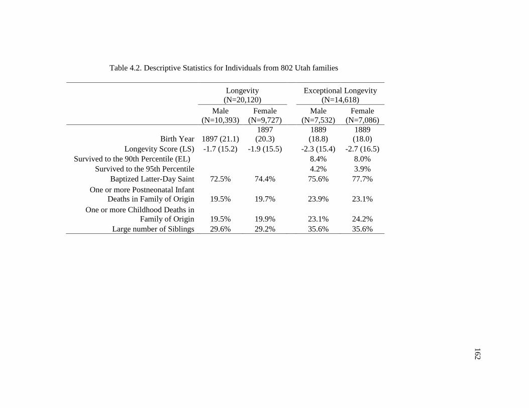
128
Table 4.2. Descriptive Statistics for Individuals from 802 Utah families
Longevity
(N=20,120)
Exceptional Longevity
(N=14,618)
Male
(N=10,393)
Female
(N=9,727)
Male
(N=7,532)
Female
(N=7,086)
Birth Year 1897 (21.1)
1897
(20.3)
1889
(18.8)
1889
(18.0)
Longevity Score (LS) -1.7 (15.2) -1.9 (15.5)
-2.3 (15.4) -2.7 (16.5)
Survived to the 90th Percentile (EL)
8.4% 8.0%
Survived to the 95th Percentile
4.2% 3.9%
Baptized Latter-Day Saint 72.5% 74.4%
75.6% 77.7%
One or more Postneonatal Infant
Deaths in Family of Origin 19.5% 19.7%
23.9% 23.1%
One or more Childhood Deaths in
Family of Origin 19.5% 19.9%
23.1% 24.2%
Large number of Siblings 29.6% 29.2% 35.6% 35.6%
162

129
Table 4.3. Summary of the Results Obtained for Polygenic Models of LS (N=20,120)
163

128
Table 4.4. Summary of the Results Obtained for Polygenic Models of EL
164

165
Figure 4.1. Hypotheses for GxE interactions: Expected. The expected phenotypic
variation in a normal environment.

166
Figure 4.2. Hypotheses for GxE interactions: Triggering. A triggering GxE interaction in
an adverse environment.
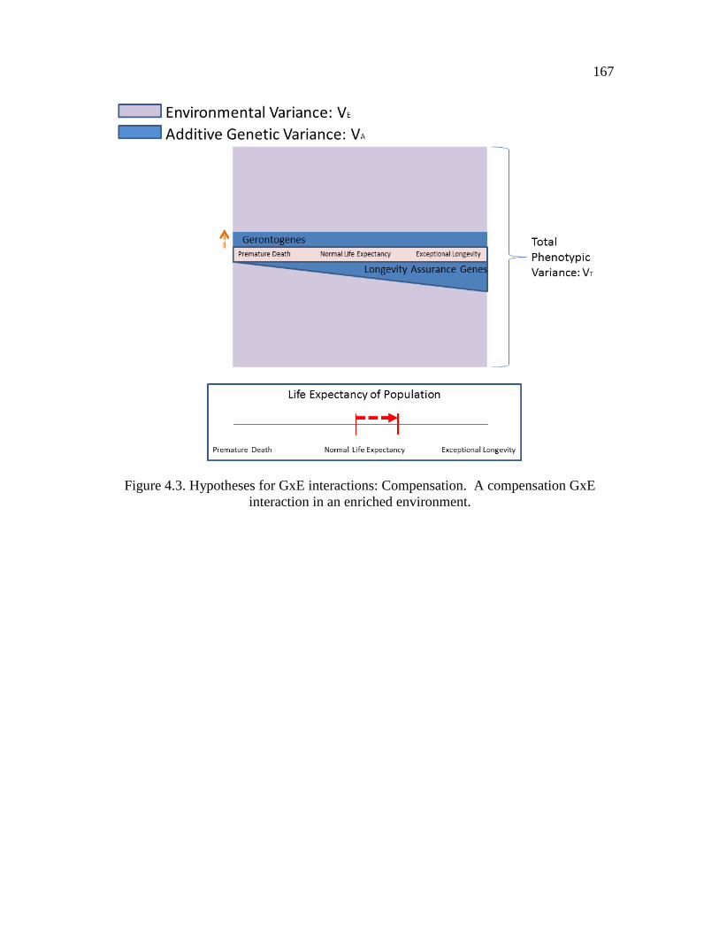
167
Figure 4.3. Hypotheses for GxE interactions: Compensation. A compensation GxE
interaction in an enriched environment.

168
Figure 4.4. Hypotheses for GxE interactions: Enhancement. An enhancement interaction
in an enriched environment.

169
Figure 4.5. Predicted values of survival to the 50th and 90th percentiles by gender and
birth year. Panels A and B show the estimates for male 50th
and 90th
percentile estimates,
respectively. Panels C and D show estimates for female 50th
and
90th
percentiles, respectively.

170
Figure 4.6. Distribution of calculated longevity for individuals born between 1850 and
1927 and surviving to age 30. Panel A shows the distribution for the cohort used in the
baseline survival analysis (N=685,949). Panel B shows the distribution for the
heritability sample (N=20,120).
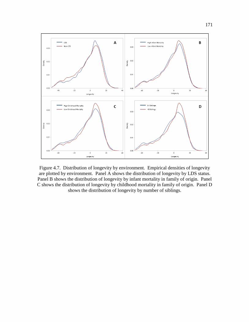
171
Figure 4.7. Distribution of longevity by environment. Empirical densities of longevity
are plotted by environment. Panel A shows the distribution of longevity by LDS status.
Panel B shows the distribution of longevity by infant mortality in family of origin. Panel
C shows the distribution of longevity by childhood mortality in family of origin. Panel D
shows the distribution of longevity by number of siblings.
CHAPTER 5
CONCLUSION
This dissertation investigated heterogeneity in patterns of aging and the factors
throughout the life course that shape them. By focusing on variability within the
population we are able to provide a clearer picture of how circumstances throughout the
life course affect the way individuals age. We found that the paths to disease and
longevity are diverse and that early and midlife factors play an important role in
determining later life health and longevity. Our results support a wide body of literature
showing that morbidity is not an inevitable consequence of aging, even in the oldest old
population, but is shaped by the historical circumstances and social environments that we
live in. This study offered innovative and significant contributions to the understanding
of biological and socioenvironmental determinants of aging. Our research sought to
disentangle the biological and temporal sources of trends in cancer incidence,
investigating the possible social and physiological effects of fertility history on
comorbidity trajectories after age 65, and studying the heterogeneity in the heritable
components of the total phenotypic variation in longevity across early life family and
social environments.

173
Fully understanding the sources of heterogeneity in the patterns of aging and
longevity using only measures of the early life or proximate environment is an impossible
endeavor because the biological functioning of an individual is dependent upon a vast
array of circumstances from birth to death. Healthy aging and longevity phenotypes
should be characterized as plastic and not one fixed at or near the time of birth. Trends in
cancer incidence in the oldest old are sensitive to period and cohort influences. Fertility
history affects disease progression later in life and these effects are independent of early
life circumstances, including a family history of longevity. These findings suggest that
childhood is not the only malleable period in the life course; midlife circumstances may
also alter the trajectories of age related degeneration. The moderate heritability of
exceptional longevity is evidence that genes are not the only factor contributing to this
phenotype. There is also some evidence that heritability of longevity is sensitive to
childhood environments. Therefore, it is essential to consider how events throughout the
life course and their interrelationships influence aging and longevity.
Little is known about age-specific disease incidence and prevalence among the
oldest old (Boscoe, 2008; Christensen, Johnson, & Vaupel, 2006). This study highlighted
the heterogeneity of disease patterns in this population by analyzing age, period, and
cohort (APC) effects on cancer incidence in the oldest old and individual trajectories of
disease for two cohorts over an 18 year period. We found significant evidence of
variance in disease patterns for this population and evidence that social context and
events throughout the life course influence patterns of disease even for the exceptionally
long lived. The APC analyses provided evidence that the decline in cancer incidence for
this age group is not strictly related to biological phenomenon. Characterizing
trajectories of disease up to age 91 in the young-old cohort and 101 in the old-old cohort

174
provides evidence that even into these advance ages the patterns of disease are diverse.
We found that there are distinct heterogeneous patterns of comorbidity that range from a
robust group, escaping major morbid conditions for the majority of the observation
period, to a frail group characterized by high comorbidity throughout the entire period of
observation. These findings underscore the importance of more rigorous and
interdisciplinary research into the biological and social underpinnings of disease for this
rapidly increasing segment of the population.
It is important to consider how mortality selection shapes age-related patterns of
disease. While it is clear that longevity is only moderately heritable at extreme ages,
heritability also increases with age. This suggests that there may be genetic variants that
are protective against deleterious genetic and environmental effects. The buffering
mechanisms in aging hypothesis suggests that longevity genes buffer against the harmful
effects of deleterious genotypes (Huffman et al., 2012). The decline in cancer incidence
above age 90 also suggests that individuals reaching the extreme ends of longevity may
be less susceptible to disease. However, the diverse patterns of comorbidity experience
provide evidence that longevity is not synonymous with disease free living.
Future Research
Sociological and demographic studies of aging and longevity should inform and
be informed by the fields of genetics, epidemiology, and biology. More attention should
be given to uncovering genetic and biological pathways to health and their interaction
with the social environment. The integration of theories of aging from multiple
disciplines is essential to unraveling the secrets of this multifactorial process. It is
difficult to identify the mechanisms that separate the exceptionally longevous, salubrious

175
individuals from those with multiple morbidities and a shortened life-span; however, it is
clear that these differences cannot be wholly explained by biological or social
mechanisms. Therefore, future demographic work should continue to improve upon the
specification of biological and social paths to health outcomes.
The studies presented in this dissertation utilized a range of tools to describe
aging and longevity trends in the populations. Each of these tools has unique aspects that
can be leveraged to further advance the field of aging and longevity. Age, period, and
cohort (APC) analyses can be considered descriptive. It is not possible to make causal
statement as to what factors led to the observed trends. However, this is not sufficient
reason for demographers to abandon APC analyses. It is the ability to describe the
multidimensionality of morbidity and mortality trends that give these analyses so much
power and point to domains that may hold some of the answers to fundamental questions
about the origins of longevity.
Making definitive statements about age-related trends using cross-sectional data
or longitudinal data from a single cohort is a dangerous practice. The observed trends in
cross-sectional data may be confounded by cohort differences in exposure, while
longitudinal data from a small number of cohorts are not generalizable because the
observed patterns may be specific to these cohorts. Therefore, we advocate a
decomposition approach to understanding the underlying factors of disease by first
defining age, period, and cohort effects of morbidity and cause-specific mortality. This
first step does not provide a complete explanation for the trends, but it helps to elucidate
what needs to be explained. The second step then involves further investigating the
components and interrelationships in order to make more definitive causal statements
about the disease process. Investigating population trends using this strategy can shed

176
considerable light on the ways that social environments intersect with biological factors
determining disease.
The use of group-based trajectory modeling to construct heterogeneous patterns of
aging is extremely informative to the studies of aging and longevity. It has become clear
that there is not a linear pattern of decline in physiological function determined by
chronological age at the population or individual level. Assessing unique patterns of
disease and disability experience give us a more realistic picture of how people age. We
also have much to learn about which experiences throughout the life course contribute to
specific patterns of aging. Other sources of early life information, such as linked
Decennial Censuses and military service records, will be available as part of the UPDB
infrastructure in the near future. This will allow for further investigation into the
association between early and midlife events and later life morbidity. We also suggest
that study is warranted for investigating specific diseases or groups of disease (rather than
composite measures only) with similar biological underpinnings to further understand the
association between fertility and later life health.
Exploring gene-environment (GxE) interactions using a multigenerational
database with information on early and midlife conditions is a fruitful approach to
understanding how the social environment affects later life health. Not only can the
study presented here be expanded to include other environments, but it can also be
expanded to examine variation in heritability of other aging phenotypes. For example,
we identified a group of robust individuals that experienced low levels of disease over an
18 year period in the trajectory analysis. It would be interesting to see if there is evidence
of heritability of a “robust” phenotype. Other ways of investigating GxE interactions
should also be explored. There is potential for using biomarker data, including APO-E

177
and telomere length, to investigate the possibility of environmentally altered phenotypic
expression.
Population projections that assume future gains in healthy life expectancy and life
expectancy in general will remain on a fixed path should be viewed with caution because
life expectancy is sensitive to both historical and current sociological context. This is not
to say that future improvements in healthy life expectancy and life expectancy in general
are impossible, but they are dependent upon factors that are still not well understood.
Also, much more research needs to be conducted in order to understand disease
trajectories specific to the oldest old population. We cannot plan for proper care of this
rapidly increasing population when we know so little about their healthcare needs.
Conclusions
This research contributes to a growing body of literature that draws attention to
effects of early life circumstances on later life health. Health policies should be aimed at
promoting the well-being of individuals throughout the life course. This research
specifically highlights the importance of maternal well-being during childbearing years.
The future health of women is not only affected while they are in their reproductive
years, but it has been shown to affect the health of her offspring (Gluckman & Hanson,
2005). Therefore special attention should be given to this sensitive period that may alter
the health of multiple generations. This research also highlights the importance of social
context throughout the life course in determining later life health. Health risks are
created and maintained by social structures and more work must be done to understand
the social disparities that lead to disparities in health later in life and possibly across
generations. As a more individuals advance into the oldest old ages, we will need to

178
review health and cancer screening recommendations of the past. The view that this age
group is too frail or has too many comorbid conditions should be reconsidered (Østbye,
Greenberg, Taylor, & Lee, 2003) based on trends in cancer incidence for this population.
Understanding the sources of variation in patterns of aging is important for
creating accurate population predictions, identifying at risk populations that may benefit
from public health interventions, and characterizing the process of aging in a diverse
population. Rather than focusing on the average life expectancy or healthy life
expectancy of the population and their trends over time, we should be focusing on the
variability of these measures within a population and changes in the sources of variation
over time. This is a subtle but important difference. By elucidating mechanisms that
lead to heterogeneous patterns of aging, we can not only gain more insight into the
determinants of aging, but focus on the factors that have the largest impact. Health
policy should be focused on not only curing ailments once they present themselves, but
more importantly, preventing them throughout the life course.
179
References
Boscoe, F. P. (2008). Subdividing the age group of 85 years and older to improve US
disease reporting. American Journal of Public Health, 98(7), 1167-1170. doi:
10.2105/ajph.2008.133900
Christensen, K., Johnson, T. E., & Vaupel, J. W. (2006). The quest for genetic
determinants of human longevity: Challenges and insights. Nat Rev Genet, 7(6),
436-448.
Gluckman, P. D., & Hanson, M. (2005). The fetal matrix: Evolution, development, and
disease. Cambridge: Cambridge Univ Press.
Huffman, D. M., Deelen, J., Ye, K., Bergman, A., Slagboom, E. P., Barzilai, N., &
Atzmon, G. (2012). Distinguishing between longevity and buffered-deleterious
genotypes for exceptional human longevity: The case of the MTP gene. The
Journals of Gerontology Series A: Biological Sciences and Medical Sciences,
67(11), 1153-1160. doi: 10.1093/gerona/gls103
Østbye, T., Greenberg, G. N., Taylor, D. H., & Lee, A. M. M. (2003). Screening
mammography and pap tests among older American women 1996–2000: Results
from the Health and Retirement Study (HRS) and Asset and Health Dynamics
Among the Oldest Old (AHEAD). The Annals of Family Medicine, 1(4), 209-217.
doi: 10.1370/afm.54