understanding the disharmony between dropout and batch ... · dropout =1 :l ; bn 0 20 40 60 80 100...

Understanding the Disharmony between Dropout and Batch Normalization byVariance Shift

Xiang Li 1 Shuo Chen 1 Xiaolin Hu 2 Jian Yang 1

Abstract

This paper first answers the question “why dothe two most powerful techniques Dropout andBatch Normalization (BN) often lead to a worseperformance when they are combined together?”in both theoretical and statistical aspects. The-oretically, we find that Dropout would shift thevariance of a specific neural unit when we transferthe state of that network from train to test. How-ever, BN would maintain its statistical variance,which is accumulated from the entire learningprocedure, in the test phase. The inconsistencyof that variance (we name this scheme as “vari-ance shift”) causes the unstable numerical behav-ior in inference that leads to more erroneous pre-dictions finally, when applying Dropout beforeBN. Thorough experiments on DenseNet, ResNet,ResNeXt and Wide ResNet confirm our findings.According to the uncovered mechanism, we nextexplore several strategies that modifies Dropoutand try to overcome the limitations of their com-bination by avoiding the variance shift risks.

1. Introduction(Srivastava et al., 2014) brought Dropout as a simple way toprevent neural networks from overfitting. It has been provedto be significantly effective over a large range of machinelearning areas, such as image classification (Szegedy et al.,2015), speech recognition (Hannun et al., 2014) and evennatural language processing (Kim et al., 2016). Beforethe birth of Batch Normalization, it became a necessity ofalmost all the state-of-the-art networks and successfullyboosted their performances against overfitting risks, despiteits amazing simplicity.

(Ioffe & Szegedy, 2015) demonstrated Batch Normaliza-

1DeepInsight@PCALab, Nanjing University of Science andTechnology, China 2Tsinghua National Laboratory for Informa-tion Science and Technology (TNList) Department of ComputerScience and Technology, Tsinghua University, China. Correspon-dence to: Xiang Li <[email protected]>.

𝑋 = 𝑥 𝑋 =𝑋−𝐸𝑀𝑜𝑣𝑖𝑛𝑔 (𝑋)

𝑉𝑎𝑟𝑀𝑜𝑣𝑖𝑛𝑔 𝑋 +𝜀𝑋

𝑉𝑎𝑟𝑇𝑟𝑎𝑖𝑛 𝑋 =1

𝑝

𝑉𝑎𝑟𝑇𝑒𝑠𝑡 𝑋 = 1

𝑉𝑎𝑟𝑀𝑜𝑣𝑖𝑛𝑔 𝑋 = 𝐸(1

𝑝)

𝑉𝑎𝑟𝑀𝑜𝑣𝑖𝑛𝑔 𝑋 = 𝐸(1

𝑝)

𝑥~𝒩(0,1)

Train Mode

Test Mode

𝑋 = 𝑎1

𝑝𝑥 𝑋𝑥~𝒩(0,1)

𝜇 = 𝐸 𝑋 , 𝜎2 = 𝑉𝑎𝑟 𝑋 , 𝑋 =𝑋 − 𝜇

𝜎2 + 𝜀𝐸𝑀𝑜𝑣𝑖𝑛𝑔 𝑋 ← 𝐸(𝜇) 𝑉𝑎𝑟𝑀𝑜𝑣𝑖𝑛𝑔 𝑋 ← 𝐸(𝜎2)

Dropout 𝑎~Bernoulli(𝑝) BN

0 20 40 60 80 100

BN layer index on DenseNet trained on CIFAR100

0.5

1.0

1.5

2.0

2.5

3.0

3.5

max(real_var i

moving_var i,m

oving_var i

real_var i

)

Test Acc 77.42%, No Dropout in each bottleneckTest Acc 68.55%, Dropout 0.5 in each bottleneck

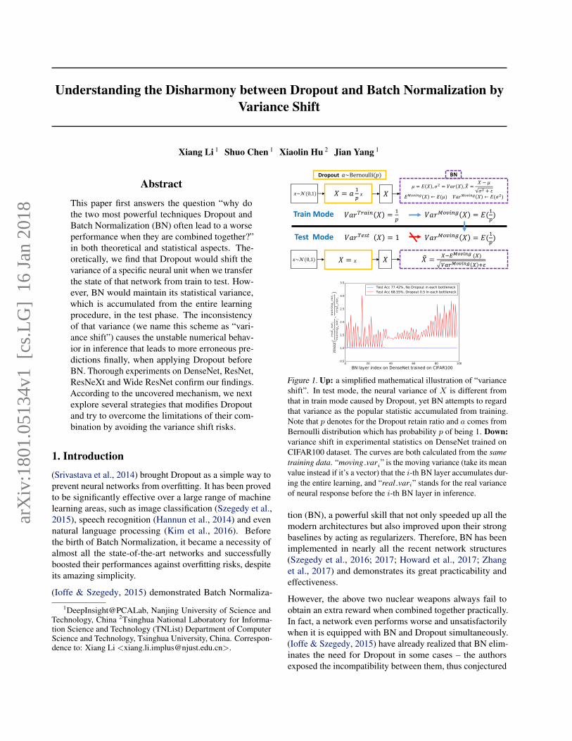
Figure 1. Up: a simplified mathematical illustration of “varianceshift”. In test mode, the neural variance of X is different fromthat in train mode caused by Dropout, yet BN attempts to regardthat variance as the popular statistic accumulated from training.Note that p denotes for the Dropout retain ratio and a comes fromBernoulli distribution which has probability p of being 1. Down:variance shift in experimental statistics on DenseNet trained onCIFAR100 dataset. The curves are both calculated from the sametraining data. “moving vari” is the moving variance (take its meanvalue instead if it’s a vector) that the i-th BN layer accumulates dur-ing the entire learning, and “real vari” stands for the real varianceof neural response before the i-th BN layer in inference.

tion (BN), a powerful skill that not only speeded up all themodern architectures but also improved upon their strongbaselines by acting as regularizers. Therefore, BN has beenimplemented in nearly all the recent network structures(Szegedy et al., 2016; 2017; Howard et al., 2017; Zhanget al., 2017) and demonstrates its great practicability andeffectiveness.

However, the above two nuclear weapons always fail toobtain an extra reward when combined together practically.In fact, a network even performs worse and unsatisfactorilywhen it is equipped with BN and Dropout simultaneously.(Ioffe & Szegedy, 2015) have already realized that BN elim-inates the need for Dropout in some cases – the authorsexposed the incompatibility between them, thus conjectured

arX

iv:1

801.

0513

4v1

[cs

.LG

] 1

6 Ja

n 20

18

Understanding the Disharmony between Dropout and Batch Normalization by Variance Shift

that BN provides similar regularization benefits as Dropoutintuitively. More evidences are provided in the modern ar-chitectures such as ResNet (He et al., 2016a;b), ResNeXt(Xie et al., 2017), DenseNet (Huang et al., 2016), wherethe best performances are all obtained by BN with the ab-sence of Dropout. Interestingly, a recent study Wide ResNet(WRN) (Zagoruyko & Komodakis, 2016) show that it ispositive for Dropout to be applied in the WRN design witha large feature dimension. So far, previous clues leave us amystery about the confusing and complicated relationshipbetween Dropout and BN. Why do they conflict in most ofthe common architectures? Why do they cooperate friendlysometimes as in WRN?

We discover the key to understand the disharmony betweenDropout and BN is the inconsistent behaviors of neural vari-ance during the switch of networks’ state. Considering oneneural response X as illustrated in Figure 1, when the statechanges from train to test, Dropout would scale the responseby its Dropout retain ratio (i.e. p) that actually changes theneural variance as in learning, yet BN still maintains itsstatistical moving variance of X . This mismatch of variancecould lead to a numerical instability (see red curve in Fig-ure 1). As the signals go deeper, the numerical deviation onthe final predictions may amplify, which drops the system’speformance. We name this scheme as “variance shift” forsimplicity. Instead, without Dropout, the real neural vari-ances in inference would appear very closely to the movingones accumulated by BN (see blue curve in Figure 1), whichis also preserved with a higher test accuracy.

Theoretically, we deduced the “variance shift” under twogeneral conditions, and found a satisfied explanation for theaforementioned mystery between Dropout and BN. Further,a large range of experimental statistics from four modernnetworks (i.e., PreResNet (He et al., 2016b), ResNeXt (Xieet al., 2017), DenseNet (Huang et al., 2016), Wide ResNet(Zagoruyko & Komodakis, 2016)) on the CIFAR10/100datasets verified our findings as expected.

Since the central reason for their performance drop wasdiscovered, we adopted two strategies that explored thepossibilities to overcome the limitation of their combination.One was to apply Dropout after all BN layers and anotherwas to modify the formula of Dropout and made it lesssensitive to variance. By avoiding the variance shift risks,most of them worked well and achieved extra improvements.

2. Related Work and PreliminariesDropout (Srivastava et al., 2014) can be interpreted as away of regularizing a neural network by adding noise to itshidden units. Specifically, it involves multiplying hiddenactivations by Bernoulli distributed random variables whichtake the value 1 with probability p (0 ≤ p ≤ 1) and 0

otherwise1. Importantly, the test scheme is quite differentfrom the train. During training, the information flow goesthrough the dynamic sub-network. At test time, the neuralresponses are scaled by the Dropout retain ratio, in orderto approximate an equally weighted geometric mean of thepredictions of an exponential number of learned models thatshare parameters. Consider a feature vector x = (x1 . . . xd)with channel dimension d. Note that this vector could bea part (one location) of convolutional feature-map or theoutput of the fully connected layer, i.e., it doesnot matterwhich type of network it lies in. If we apply Dropout on x,for one unit xk, k = 1 . . . d, in the train phase, it is:

xk = akxk, (1)

where ak ∼ P that comes from the Bernoulli distribution:

P (ak) =

{1− p, ak = 0p, ak = 1

, (2)

and a = (a1 . . . ad) is a vector of independent Bernoullirandom variables. At test time for Dropout, one shouldscale down the weights by multiplying them by a factorof p. As introduced in (Srivastava et al., 2014), anotherway to achieve the same effect is to scale up the retainedactivations by multiplying by 1

p at training time and notmodifying the weights at test time. It is more popular onpractical implementations, thus we employ this formula ofDropout in both analyses and experiments. Therefore, thehidden activation in the train phase would be:

xk = ak1

pxk, (3)

whilst in inference it would be simple like: xk = xk.

Batch Normalization (BN) (Ioffe & Szegedy, 2015) pro-poses a deterministic information flow by normalizingeach neuron into zero mean and unit variance. Consid-ering values of x (for clarity, x ≡ xk) over a mini-batch:B = {x(1)...(m)}2 with m instances, we have the form of“normalize” part:

µ =1

m

m∑i=1

x(i), σ2 =1

m

m∑i=1

(x(i) − µ)2, x(i) = x(i) − µ√σ2 + ε

,

(4)where µ and σ2 would participate in the backpropagation.The normalization of activations that depends on the mini-batch allows efficient training, but is neither necessary nordesirable during inference. Therefore, BN accumulatesthe moving averages of neural means and variances duringlearning to track the accuracy of a model as it trains:

EMoving(x)← EB(µ), V arMoving(x)← E

′

B(σ2), (5)

1p denotes for the Dropout retain ratio and (1− p) denotes forthe drop ratio in this paper.

2Note that we donot consider the “scale and shift” part in BNbecause the key of “variance shift” exists in its “normalize” part.


whereEB(µ) denotes for the expectation of µ from multipletraining mini-batches B and E

′

B(σ2) denotes for the expec-

tation of the unbiased variance estimate (i.e., mm−1 ·EB(σ

2))over multiple training mini-batches. They are all obtainedby implementations of moving averages (Ioffe & Szegedy,2015) and are fixed for linear transform during inference:

x =x− EMoving(x)√V arMoving(x) + ε

. (6)

3. Theoretical AnalysesFrom the preliminaries, one could notice that Dropout onlyensures an “equally weighted geometric mean of the pre-dictions of an exponential number of learned models” bythe approximation from its test policy, as introduced in theoriginal paper (Srivastava et al., 2014). This scheme posesthe variance of the hidden units unexplored in a Dropoutmodel. Therefore, the central idea is to investigate the vari-ance of the neural response before a BN layer, where theDropout is previously applied. This could be attributedinto two cases generally, as shown in Figure 2. In case(a), the BN layer is directly subsequent to the Dropoutlayer and we only need to consider one neural responseX = ak

1pxk, k = 1 . . . d in train phase and X = xk in test

phase. In case (b), the feature vector x = (x1 . . . xd) wouldbe passed into a convolutional layer (or a fully connectedlayer) to form the neural response X . We also regard itscorresponding weights (the convolutional filter or the fullyconnected weight) to be w = (w1 . . . wd), hence we getX =

∑di=1 wiai

1pxi for learning and X =

∑di=1 wixi for

test. For the ease of deduction, we assume that the inputsall come from the distribution with c mean and v variance(i.e., E(xi) = c, V ar(xi) = v, i = 1 . . . d, v > 0) and wealso start by studying the linear regime. We let the ai andxi be mutually independent, considering the property ofDropout. Due to the aforementioned definition, ai and ajare mutually independent as well.

Dropout BN

DropoutConvolutional /Fully Connected

BN

𝚾

𝚾

(a)

(b) 𝑋

𝑋

Dropout [inference: 𝑋 =𝑑

𝑚Χ] BN [inference: 𝑋 =

𝑋−𝐸𝑀𝑜𝑣𝑖𝑛𝑔 [𝑋]

𝑉𝑎𝑟𝑀𝑜𝑣𝑖𝑛𝑔 𝑋 +𝜀]𝑋

𝑉𝑎𝑟𝑇𝑟𝑎𝑖𝑛 𝑋 = 1 − 𝑑/𝑚

𝑉𝑎𝑟𝑇𝑒𝑠𝑡 𝑋 = 1 − 𝑑/𝑚 2

𝑉𝑎𝑟𝑀𝑜𝑣𝑖𝑛𝑔 𝑋 = 𝐸 1 − 𝑑/𝑚

𝑉𝑎𝑟𝑀𝑜𝑣𝑖𝑛𝑔 𝑋 = 𝐸 1 − 𝑑/𝑚

Χ

Χ~𝑁(0,1)

Χ~𝑁(0,1) ≠

Train Mode

Test Mode

Figure 2. Two cases for analyzing variance shift.

Figure 2 (a)

Following the paradigms above, we have V arTrain(X) as:

V arTrain(X) = V ar(ak1

pxk) = E((ak

1

pxk)

2)− E2(ak1

pxk)

=1

p2E(a2k)E(x2k)−

1

p2(E(ak)E(xk))

2 =1

p(c2 + v)− c2

(7)

In inference, BN keeps the moving average of variance (i.e.,E

′

B(1p (c

2+v)−c2)) fixed. In another word, BN wishes thatthe variance of neural response X , which comes from theinput images, is supposed to be close toE

′

B(1p (c

2+v)−c2).However, Dropout breaks the harmony when it comes toits test stage by having X = xk to get V arTest(X) =V ar(xk) = v. If putting V arTest(X) into the unbiasedvariance estimate, it would become E

′

B(v) which is obvi-ously different from the popular statisticE

′

B(1p (c

2+v)−c2)of BN during training when Dropout (p < 1) is applied.Therefore, the shift ratio is obtained:

4(p) =V arTest(X)

V arTrain(X)=

v1p (c

2 + v)− c2(8)

In case (a), the variance shift happens via a coefficient4(p) ≤ 1. Since modern neural networks carry a deepfeedforward topologic structure, previous deviate numericalmanipulations could lead to more uncontrollable numericaloutputs of subsequent layers (Figure 1). It brings the chainreaction of amplified shift of variances (even affects themeans further) in every BN layers sequentially as the net-works go deeper. We would show that it directly leads to adislocation of final predictions and makes the system sufferfrom a performance drop later in the statistical experimentalpart (e.g., Figure 4, 6 in Section 4).

In this design (i.e., BN directly follows Dropout), if we wantto alleviate the variance shift risks, i.e.,4(p)→ 1, the onlything we can do is to eliminate Dropout and set the Dropoutretain ratio p → 1. Fortunately, the architectures whereDropout brings benefits (e.g., in Wide ResNet) donot followthis type of arrangement. In fact, they adopt the case (b) inFigure 2, which is more common in practice, and we woulddescribe it in details next.

Figure 2 (b)

At this time,X would be obtained by∑di=1 wiai

1pxi, where

w denotes for the corresponding weights that act on the fea-ture vector x, along with the Dropout applied. For the easeof deduction, we assume that in the very later epoch of train-ing, the weights of w remains constant given the gradientsbecome significantly close to zero. Similarly, we can writeV arTrain(X) by following the formula of variance:

V arTrain(X) = Cov(

d∑i=1

wiai1

pxi,

d∑i=1

wiai1

pxi)

=1

p2

d∑i=1

(wi)2V ar(aixi)

+1

p2

d∑i=1

d∑j 6=i

ρaxi,jwiwj√V ar(aixi)

√V ar(ajxj)

= (1

p(c2 + v)− c2)(

d∑i=1

w2i + ρax

d∑i=1

d∑j 6=i

wiwj),

(9)


0 20 40 60 80 100Convolutional Layer Index of Networks Trained on CIFAR10

0.0

0.1

0.2

0.3

0.4

0.5

0.6

0.7

0.8

0.9

1.0

Mean o

f (cos

(θ))

2

PreResNetResNeXtWRNDenseNet

0 20 40 60 80 100Convolutional Layer Index of Networks Trained on CIFAR100

0.0

0.1

0.2

0.3

0.4

0.5

0.6

0.7

0.8

0.9

1.0

Mean o

f (cos

(θ))

2


0 1000 2000 3000 4000 5000 6000Weight Dimension d of Convolutional Filter Trained on CIFAR10

0

20

40

60

80

100

120

140

Mean o

f d(cos

(θ))

2


0 1000 2000 3000 4000 5000 6000Weight Dimension d of Convolutional Filter Trained on CIFAR100

0

20

40

60

80

100

Mean o

f d(cos

(θ))

2


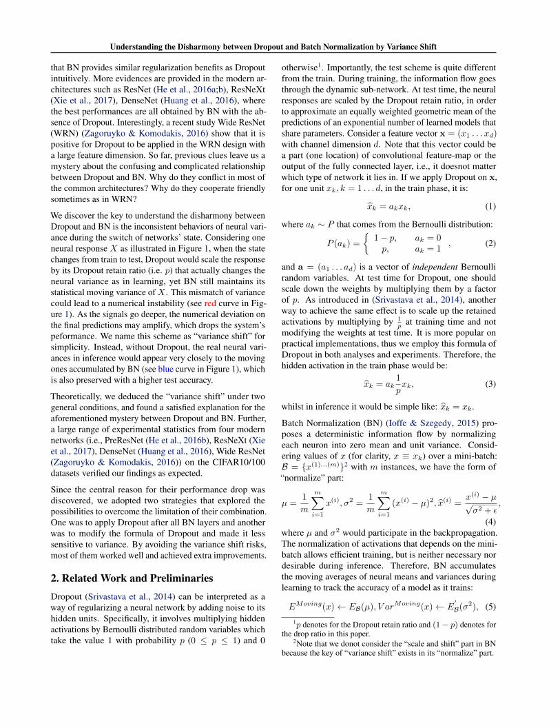
Figure 3. Statistical mean values of (cos θ)2 and d(cos θ)2. These four modern architectures are trained without Dropout on CIFAR10and CIFAR100 respectively. We observe that (cos θ)2 lies in (0.01, 0.10) approximately in every network structure and various datasets.Interestingly, the term d(cos θ)2 in WRN is significantly bigger than those on other networks mainly due to its larger channel width d.

where ρaxi,j =Cov(aixi,ajxj)√

V ar(aixi)√V ar(ajxj)

∈ [−1, 1]. For the

ease of deduction, we simplify all the linear correlationcoefficients to be the same as a constant ρax ∼= ρaxi,j ,∀i, j =1 . . . d, i 6= j. Similarly, V arTest(X) is obtained:

V arTest(X) = V ar(

d∑i=1

wixi) = Cov(d∑i=1

wixi,d∑i=1

wixi)

=

d∑i=1

w2i v +

d∑i=1

d∑j 6=i

ρxi,jwiwj√v√v

= v(

d∑i=1

w2i + ρx

d∑i=1

d∑j 6=i

wiwj),

(10)where ρxi,j =

Cov(xi,xj)√V ar(xi)

√V ar(xj)

∈ [−1, 1], and we also

have a constant ρx ∼= ρxi,j ,∀i, j = 1 . . . d, i 6= j. Since aiand xi, ai and aj are mutually independent, we can get therelationship between ρax and ρx:

ρax ∼= ρaxi,j =Cov(aixi, ajxj)√

V ar(aixi)√V ar(ajxj)

=p2Cov(xi, xj)

p(c2+v)−p2c2v

√V ar(xi)

√V ar(xj)

=v

1p (c

2 + v)− c2ρxi,j∼=

v1p (c

2 + v)− c2ρx.

(11)

According to Equation (9), (10) and (11), we can write thevariance shift V arTest(X)

V arTrain(X)as:

v(∑di=1 w

2i + ρx

∑di=1

∑dj 6=i wiwj)

( 1p (c2 + v)− c2)(

∑di=1 w

2i + ρax

∑di=1

∑dj 6=i wiwj)

=v∑di=1 w

2i + vρx

∑di=1

∑dj 6=i wiwj

( 1p (c2 + v)− c2)

∑di=1 w

2i + vρx

∑di=1

∑dj 6=i wiwj

=v + vρx((

∑di=1 wi)

2 −∑di=1 w

2i )/∑di=1 w

2i

1p (c

2 + v)− c2 + vρx((∑di=1 wi)

2 −∑di=1 w

2i )/∑di=1 w

2i

=v + vρx(d(cos θ)2 − 1)

1p (c

2 + v)− c2 + vρx(d(cos θ)2 − 1),

(12)

Table 1. Statistical means of (cos θ)2 and d(cos θ)2 over all theconvolutional layers on four representative networks.

Networks CIFAR10 CIFAR100(cos θ)2 d(cos θ)2 (cos θ)2 d(cos θ)2

PreResNet 0.03546 2.91827 0.03169 2.59925ResNeXt 0.02244 14.78266 0.02468 14.72835WRN 0.02292 52.73550 0.02118 44.31261DenseNet 0.01538 3.83390 0.01390 3.43325

where (cos θ)2 comes from the expression:

(∑di=1 wi)

2

d ·∑di=1 w

2i

= (

∑di=1 1 · wi√∑d

i=1 12

√∑di=1 w

2i

)

2

= (cos θ)2,

(13)and θ denotes for the angle between vector w and vector(1 . . . 1)︸︷︷︸

m

. To prove that d(cos θ)2 scales approximately lin-

ear to d, we made rich calculations w.r.t the term d(cos θ)2

and (cos θ)2 on four modern architectures3 trained on CI-FAR10/100 datasets (Table 1 and Figure 3). Based on Table1 and Figure 3, we observe that (cos θ)2 lies in (0.01, 0.10)stably in every network and various datasets whilst d(cos θ)2

tends to increase in parallel when d grows. From Equa-tion (12), the inequation V arTest(X) 6= V arTrain(X)holds when p < 1. If we want V arTest(X) to approachV arTrain(X), we need this term

4(p, d) =V arTest(X)

V arTrain(X)=

vρx(d(cos θ)2 − 1) + v

vρx(d(cos θ)2 − 1) + 1p (c

2 + v)− c2

=vρx + v(1−ρx)

d(cos θ)2

vρx +( 1p−1)c2+v(

1p−ρx)

d(cos θ)2

(14)to approach 1. There are two ways to achieve4(p, d)→ 1:

• p→ 1: maximizing the Dropout retain ratio p (ideallyup to 1 which means Dropout is totally eliminated);

• d→∞: growing the width of channel exactly as theWide ResNet did to enlarge d.

3For the convolutional filters which have larger than 1 filtersize as k × k, k > 1, we vectorise them by expanding its channelwidth d to d× k × k while maintaining all the weights.


4. Statistical ExperimentsWe conduct extensive statistical experiments to check thecorrectness of above deduction in this section. Four modernarchitectures including DenseNet (Huang et al., 2016), Pre-ResNet (He et al., 2016b), ResNeXt (Xie et al., 2017) andWide ResNet (WRN) (Zagoruyko & Komodakis, 2016) areadopted on the CIFAR10 and CIFAR100 datasets.

Datasets. The two CIFAR datasets (Krizhevsky & Hinton,2009) consist of colored natural scence images, with 32×32pixel each. The train and test sets contain 50k images and10k images respectively. CIFAR10 (C10) has 10 classesand CIFAR100 (C100) has 100. For data preprocessing, wenormalize the data by using the channel means and standarddeviations. For data augmentation, we adopt a standardscheme that is widely used in (He et al., 2016b; Huanget al., 2016; Larsson et al., 2016; Lin et al., 2013; Lee et al.,2015; Springenberg et al., 2014; Srivastava et al., 2015): theimages are first zero-padded with 4 pixels on each side, thena 32×32 crop is randomly sampled from the padded imagesand at least half of the images are horizontally flipped.

Networks with Dropout. The four modern architecturesare all chosen from the open-source codes4 written in py-torch that can reproduce the results reported in previouspapers. The details of the networks are listed in Table 2:

Table 2. Details of four modern networks in experiments. #P de-notes for the amount of model parameters.

Model #P on C10 #P on C100

PreResNet-110 1.70 M 1.77 MResNeXt-29, 8 × 64 34.43 M 34.52 MWRN-28-10 36.48 M 36.54 MDenseNet-BC (L=100, k=12) 0.77 M 0.80 M

Since the BN layers are already developed as the indispensi-ble components of their body structures, we arrange Dropoutthat follows the two cases in Figure 2:

(a) We assign all the Dropout layers only and right be-fore all the bottlenecks’ last BN layers in these four net-works, neglecting their possible Dropout implementations(as in DenseNet (Huang et al., 2016) and Wide ResNet(Zagoruyko & Komodakis, 2016)). We denote this designto be models of Dropout-(a).

(b) We follow the assignment of Dropout in Wide ResNet(Zagoruyko & Komodakis, 2016), which finally improvesWRNs’ overall performances, to place the Dropout beforethe last Convolutional layer in every bottleneck block ofPreResNet, ResNeXt and DenseNet. This scheme is denotedas Dropout-(b) models.

4Our implementations basicly follow the public code inhttps://github.com/bearpaw/pytorch-classification. The trainingdetails can also be found there. Our code for the following experi-ments would be released soon.

Statistics of variance shift. Assume a network G containsn BN layers in total. We arrange these BN layers fromshallow to deep by giving them indices that goes from 1to n accordingly. The whole statistical manipulation isconducted by following three steps:

(1) Calculate moving vari, i ∈ [1, n]: when G is traineduntil convergence, each BN layer obtains the moving aver-age of neural variance (the unbiased variance estimate) fromthe feature-map that it receives during the entire learningprocedure. We denote that variance to be moving var. Sincethe moving var for every BN layer is a vector (whose lengthis equal to the amount of channels of previous feature-map),we leverage its mean value to represent moving var instead,for a better visualization. Further, we denote moving varias the moving var of i-th BN layer.

(2) Calculate real vari, i ∈ [1, n]: after training, we fix allthe parameters of G and set its state to be the evaluationmode (hence the Dropout would apply its inference policyand BN would freeze its moving averages of means andvariances). The training data is again utilized for goingthrough G within a certain of epochs, in order to get the realexpectation of neural variances on the feature-maps beforeeach BN layer. Data augmentation is also kept to ensurethat every possible detail for calculating neural variancesremains exactly the same with training. Importantly, weadopt the same moving average algorithm to accumulatethe unbiased variance estimates. Similarly in (1), we let themean value of real variance vector be real vari before thei-th BN layer.

(3) Obtain max( real varimoving vari

,moving vari

real vari ), i ∈ [1, n]: since wefocus on the shift, the scalings are all kept above 1 by theirreciprocals if possible in purpose of a better view. VariousDropout drop ratios [0.0, 0.1, 0.3, 0.5, 0.7] are applied forclearer comparisons in Figure 4. The corresponding errorrates are also included in each column.

Agreements between analyses and experiments aboutthe relation between performance and variance shift. Inthese four columns of Figure 4, we discover that when thedrop ratio is relatively small (i.e., 0.1), the green shift curvesare all near the blue ones (i.e. models without Dropout),thus their performances are as well very close to the base-lines. It agrees with our previous deduction that wheneverin (a) or (b) case, decreasing drop ratio 1−p would alleviatethe variance shift risks. Furthermore, in Dropout-(b) models(i.e., the last two columns) we find that, for WRNs, thecurves with drop ratio 0.1, 0.3 even 0.5 approaches closerto the one with 0.0 than other networks, and they all outper-form the baselines. It also aligns with our analyses sinceWRN has a significantly larger channel dimension d, and itensures that a slightly larger p would not explode the neu-ral variance but bring the original benefits, which Dropoutcarries, back to the BN-equipped networks.


0 20 40 60 80 100 120 140 160 180

[Dropout-(a) C10] BN layer index on PreResNet

1.0

1.5

2.0

2.5

3.0

max(real_var i

moving_var i,m

oving_var i

real_var i

) Dropout 0.0Dropout 0.1Dropout 0.3Dropout 0.5Dropout 0.7

0 5 10 15 20 25 30

[Dropout-(a) C10] BN layer index on ResNeXt

1.0

1.5

2.0

2.5

3.0

max(real_var i

moving_var i,m

oving_var i

real_var i


0 5 10 15 20 25

[Dropout-(a) C10] BN layer index on WRN

1.0

1.5

2.0

2.5

3.0

max(real_var i

moving_var i,m

oving_var i

real_var i


0 20 40 60 80 100

[Dropout-(a) C10] BN layer index on DenseNet

1.0

1.5

2.0

2.5

3.0

max(real_var i

moving_var i,m

oving_var i

real_var i


0 20 40 60 80 100 120 140 160 180

[Dropout-(a) C100] BN layer index on PreResNet

1.0

1.5

2.0

2.5

3.0

max(real_var i

moving_var i,m

oving_var i

real_var i


0 5 10 15 20 25 30

[Dropout-(a) C100] BN layer index on ResNeXt

1.0

1.5

2.0

2.5

3.0

max(real_var i

moving_var i,m

oving_var i

real_var i


0 5 10 15 20 25

[Dropout-(a) C100] BN layer index on WRN

1.0

1.5

2.0

2.5

3.0

max(real_var i

moving_var i,m

oving_var i

real_var i


0 20 40 60 80 100

[Dropout-(a) C100] BN layer index on DenseNet

1.0

1.5

2.0

2.5

3.0

max(real_var i

moving_var i,m

oving_var i

real_var i


0 20 40 60 80 100 120 140 160 180

[Dropout-(b) C10] BN layer index on PreResNet

1.00

1.05

1.10

1.15

1.20

max(real_var i

moving_var i,m

oving_var i

real_var i


0 5 10 15 20 25 30

[Dropout-(b) C10] BN layer index on ResNeXt

1.00

1.05

1.10

1.15

1.20

max(real_var i

moving_var i,m

oving_var i

real_var i


0 5 10 15 20 25

[Dropout-(b) C10] BN layer index on WRN

1.00

1.05

1.10

1.15

1.20

max(real_var i

moving_var i,m

oving_var i

real_var i


0 20 40 60 80 100

[Dropout-(b) C10] BN layer index on DenseNet

1.00

1.05

1.10

1.15

1.20

max(real_var i

moving_var i,m

oving_var i

real_var i


0 20 40 60 80 100 120 140 160 180

[Dropout-(b) C100] BN layer index on PreResNet

1.00

1.05

1.10

1.15

1.20

max(real_var i

moving_var i,m

oving_var i

real_var i


0 5 10 15 20 25 30

[Dropout-(b) C100] BN layer index on ResNeXt

1.00

1.05

1.10

1.15

1.20

max(real_var i

moving_var i,m

oving_var i

real_var i


0 5 10 15 20 25

[Dropout-(b) C100] BN layer index on WRN

1.00

1.05

1.10

1.15

1.20

max(real_var i

moving_var i,m

oving_var i

real_var i


0 20 40 60 80 100

[Dropout-(b) C100] BN layer index on DenseNet

1.00

1.05

1.10

1.15

1.20

max(real_var i

moving_var i,m

oving_var i

real_var i


PreResNet ResNeXt WRN DenseNet

Dropout-(a) C100

5

10

15

20

Err

or

rate

(%

)

0.0 0.1 0.3 0.5 0.7


Dropout-(a) C1000

5

10

15

20

25

30

35

40

Err

or

rate

(%

)

0.0 0.1 0.3 0.5 0.7


Dropout-(b) C100

1

2

3

4

5

6

7

8

Err

or

rate

(%

)

0.0 0.1 0.3 0.5 0.7


Dropout-(b) C1000

5

10

15

20

25

30

Err

or

rate

(%

)

0.0 0.1 0.3 0.5 0.7

Figure 4. See by columns. Statistical visualizations about “variance shift” on BN layers of four modern networks w.r.t: 1) Dropout type;2) Dropout drop ratio; 3) dataset, along with their test error rates (the fifth row). Obviously, WRN is less influenced by Dropout (i.e.,small variance shift) when the Dropout-(b) drop ratio ≤ 0.5, thus it even enjoys an improvement with Dropout applied before BN.

Even the training data performs inconsistently betweentrain and test mode. In addition, we also observe thatfor DenseNet and PreResNet (their channel d is relativelysmall), when their state is changed from train to test, eventhe training data cannot be kept with a coherent accuracy atlast. In inference, the variance shift happens and it leads toan avalanche effect on the numerical explosion and insta-bility in networks that finally changes the final prediction.Here we take the two models with drop ratio being 0.5 as anexample, hence demonstrate that a large amount of trainingdata would be classified inconsistently between train andtest mode, despite their same model parameters (Figure 5).

Neural responses (of last layer before softmax) for train-ing data are unstable from train to test. To get a clearerunderstanding of the numerical disturbance that the varianceshift brings finally, a bundle of images (from training data)are drawn with their neural responses before the softmaxlayer in both train stage and test stage (Figure 6). From those

pictures and their responses, we can find that with all theweights of networks fixed, only a mode transfer (from trainto test) would change the distribution of the final responseseven in the train set, and it leads to a wrong classificationconsequently. It proves that the predictions of training datadiffers between train stage and test stage when a network isequipped with Dropout layers before BN layers. Therefore,we confirm that the unstable numerical behaviors are thefundamental reasons for the performance drop.

Only an adjustment for moving means and varianceswould bring an improvement, despite all other parame-ters fixed. Given that the moving means and variances ofBN would not match the real ones during test, we attemptto adjust these values by passing the training data againunder the evaluation mode. In this way, the moving averagealgorithm (Ioffe & Szegedy, 2015) can also be applied. Af-ter shifting the moving statistics to the real ones by usingthe training data, we can have the model performed on the


0 40 80 120 160

PreResNet Dropout-(a) C100

0

20

40

60

80

100A

ccura

cy (

%)

w.r

.t e

poch

Dropout 0.0 Training data on Train ModeDropout 0.0 Training data on Test ModeDropout 0.5 Training data on Train ModeDropout 0.5 Training data on Test Mode

0 40 80 120 160 200 240 280

DenseNet Dropout-(a) C100

0

20

40

60

80

100

Acc

ura

cy (

%)

w.r

.t e

poch


30 70 110 150

PreResNet Dropout-(a) C10

82

84

86

88

90

92

94

96

98

100

Acc

ura

cy (

%)

w.r

.t e

poch


30 70 110 150 190 230 270

DenseNet Dropout-(a) C10

70

75

80

85

90

95

100

Acc

ura

cy (

%)

w.r

.t e

poch


Figure 5. Accuracy by train epochs. Curves in blue means the train of these two networks without Dropout. Curves in red denotes theDropout version of the corresponding models. These accuracies are all calculated from the training data, while the solid curve is undertrain mode and the dashed one is under evaluation mode. We observe the significant accuracy shift when a network with Dropout ratio 0.5changes its state from train to test stage, with all network parameters fixed but the test policies of Dropout and BN applied.

Figure 6. Examples of inconsistent neural responses between train mode and test mode of DenseNet Dropout-(a) 0.5 trained on CIFAR10dataset. These samples are from the training data, whilst they are correctly classified by the model during learning yet erroneously judgedin inference, despite all the fixed model parameters. Variance shift finally leads to the prediction shift that drops the performance.

Table 3. Adjust BN’s moving mean/variance by running movingaverage algorithm on training data under test mode. These numbersare all averaged from 5 parallel runnings with different randominitial seeds.

C10 Dropout-(a) Dropout-(b)0.5 0.5-Adjust 0.5 0.5-Adjust


C100 Dropout-(a) Dropout-(b)0.5 0.5-Adjust 0.5 0.5-Adjust


test set. From Table 3, All the Dropout-(a)/(b) 0.5 modelsoutperform their baselines by having their moving statisticsadjusted. Significant improvements (e.g., ∼ 2 and ∼ 4.5gains for DenseNet on CIFAR10 and on CIFAR100 respec-tively) can be observed in Dropout-(a) models. It againverifies that the drop of performance could be attributed tothe “variance shift”: a more proper popular statistics withsmaller variance shift could recall a bundle of erroneouslyclassified samples back to right ones.

Table 4. Error rates after applying Dropout after all BN layers.These numbers are all averaged from 5 parallel runnings withdifferent random initial seeds.

C10 drop ratio 0.0 0.1 0.2 0.3 0.5

PreResNet 5.02 4.96 5.01 4.94 5.03ResNeXt 3.77 3.89 3.69 3.78 3.78WRN 3.97 3.90 4.00 3.93 3.84DenseNet 4.72 4.67 4.73 4.75 4.87

C100 drop ratio 0.0 0.1 0.2 0.3 0.5


5. Strategies to Combine Them TogetherSince we get a clear knowledge about the disharmony be-tween Dropout and BN, we can easily develop several ap-proaches to combine them together, to see whether an extraimprovement could be obtained. In this section, we intro-duce two possible solutions in modifying Dropout. One isto avoid the scaling on feature-map before every BN layer,by only applying Dropout after the last BN block. Anotheris to slightly modify the formula of Dropout and make it lesssensitive to variance, which can alleviate the shift problemand stabilize the numerical behaviors.


Table 5. Error rates after applying Dropout after all BN layers onthe representative state-of-the-art models on ImageNet. Thesenumbers are averaged from 5 parallel runnings with different ran-dom initial seeds. Consistent improvements can be observed.

ImageNet drop ratiotop-1 top-5

0.0 0.2 0.0 0.2

ResNet-200 (He et al., 2016b) 21.70 21.48 5.80 5.55ResNeXt-101(Xie et al., 2017) 20.40 20.17 5.30 5.12SENet (Hu et al., 2017) 18.89 18.68 4.66 4.47

Apply Dropout after all BN layers. According to aboveanalyses, the variance shift only happens when there existsa Dropout layer before a BN layer. Therefore, the mostdirect and concise way to tackle this is to assign Dropout inthe position where the subsequent layers donot include BN.Inspired by early works that applied Dropout on the fullyconnected layers in (Krizhevsky et al., 2012), we add onlyone Dropout layer right before the softmax layer in thesefour architectures. Table 4 indicates that such a simple oper-ation could bring 0.1 improvements on CIFAR10 and reachup to 0.7 gain on CIFAR100 for DenseNet. Please notethat the last-layer Dropout performs worse on CIFAR100than on CIFAR10 generally since the training data of CI-FAR100 is insufficient and these models may suffer fromcertain underfitting risks. We also find it interesting thatWRN may not need to apply Dropout on each bottleneckblock – only a last Dropout layer could bring enough or atleast comparable benefits on CIFAR10. Additionally, wediscover that in some previous work like (Hu et al., 2017),the authors already adopted the same tips in their winningsolution on the ILSVRC 2017 Classification Competition.Since it didnot report the gain that last-layer Dropout brings,we made some additional experiments and evaluate severalstate-of-the-art models on the ImageNet (Russakovsky et al.,2015) validation set (Table 5) using a 224× 224 centre cropevaluation on each image (where the shorter edge is firstresized to 256). We observe consistent improvements whendrop ratio 0.2 is employed after all BN layers on the largescale dataset.

Change Dropout into a more variance-stable form. Thedrawbacks of vanilla Dropout lie in the weight scale duringthe test phase, which may lead to a large disturbance onstatistical variance. This clue could push us to think: if wefind a scheme that functions like Dropout but carries a lightervariance shift, we may stabilize the numerical behaviors ofneural networks, thus the final performance would probablyenjoy a possible benefit. Here we take the Figure 2 (a)case as an example for investigation where the varianceshift rate is v

1p (c

2+v)−c2 = p (we let c = 0 for simplicity).

That is, if we set the drop ratio (1− p) as 0.1, the variancewould be scaled by 0.9 when the network is transferredfrom train to test. Inspired by the original Dropout paper(Srivastava et al., 2014) where the authors also proposedanother form of Dropout that amounts to adding a Gaussian

Table 6. Apply new form of Dropout (i.e. Uout) in Dropout-(b)models. These numbers are all averaged from 5 parallel runningswith different random initial seeds.

C10 β 0.0 0.1 0.2 0.3 0.5


C100 β 0.0 0.1 0.2 0.3 0.5


distributed random variable with zero mean and standarddeviation equal to the activation of the unit, i.e., xi + xirand r ∼ N (0, 1), we modify r as a uniform distribution thatlies in [−β, β], where 0 ≤ β ≤ 1. Therefore, each hiddenactivation would be X = xi + xiri and ri ∼ U(−β, β).We name this form of Dropout as “Uout” for simplicity.With the mutually independent distribution between xi andri being hold, we apply the form X = xi + xiri, ri ∼U(−β, β) in train stage and X = xi in test mode. Similarly,in the simplified case of c = 0, we can deduce the varianceshift again as follows:V arTest(X)

V arTrain(X)=

V ar(xi)

V ar(xi + xiri)=

v

E((xi + xiri)2)

=v

E(x2i ) + 2E(x2i )E(ri) + E(x2i )E(r2i )=

3

3 + β2.

(15)Giving β as 0.1, the new variance shift rate would be 300

301 ≈0.9966777 which is much closer to 1.0 than the previous0.9 in Figure 2 (a). A list of experiments is hence employedbased on those four modern networks under Dropout-(b)settings w.r.t β (Table 6). We find that “Uout” would be lessaffected by the insufficient training data on CIFAR100 thanapplying the last-layer Dropout, which indicates a superiorproperty of stability. Except for ResNeXt, nearly all thearchitectures achieved up to 0.2 ∼ 0.3 increase of accuracyon both CIFAR10 and CIFAR100 dataset.

6. ConclusionIn this paper, we investigate the “variance shift” phe-nomenon when Dropout layers are applied before BatchNormalization on modern neural networks. We discoverthat due to their distinct test policies, neural variance wouldbe improper and shifted as the information flows in infer-ence, and it leads to the unexpected final predictions thatdrops the performance. To avoid the variance shift risks,we next explore two strategies, and they are proved to workwell in practice. We highly recommand that researcherscould take these solutions to boost their models’ perfor-mance if further improvement is desired, since their extracost is nearly free and they are easy to be implemented.


ReferencesHannun, Awni, Case, Carl, Casper, Jared, Catanzaro, Bryan,

Diamos, Greg, Elsen, Erich, Prenger, Ryan, Satheesh,Sanjeev, Sengupta, Shubho, Coates, Adam, et al. Deepspeech: Scaling up end-to-end speech recognition. arXivpreprint arXiv:1412.5567, 2014.

He, Kaiming, Zhang, Xiangyu, Ren, Shaoqing, and Sun,Jian. Deep residual learning for image recognition. InProceedings of the IEEE Conference on Computer Visionand Pattern Recognition, pp. 770–778, 2016a.

He, Kaiming, Zhang, Xiangyu, Ren, Shaoqing, and Sun,Jian. Identity mappings in deep residual networks. InEuropean Conference on Computer Vision, pp. 630–645.Springer, 2016b.

Howard, Andrew G, Zhu, Menglong, Chen, Bo,Kalenichenko, Dmitry, Wang, Weijun, Weyand, Tobias,Andreetto, Marco, and Adam, Hartwig. Mobilenets: Ef-ficient convolutional neural networks for mobile visionapplications. arXiv preprint arXiv:1704.04861, 2017.

Hu, Jie, Shen, Li, and Sun, Gang. Squeeze-and-excitationnetworks. arXiv preprint arXiv:1709.01507, 2017.

Huang, Gao, Liu, Zhuang, Weinberger, Kilian Q, andvan der Maaten, Laurens. Densely connected convolu-tional networks. arXiv preprint arXiv:1608.06993, 2016.

Ioffe, Sergey and Szegedy, Christian. Batch normalization:Accelerating deep network training by reducing internalcovariate shift. In International Conference on MachineLearning, pp. 448–456, 2015.

Kim, Yoon, Jernite, Yacine, Sontag, David, and Rush,Alexander M. Character-aware neural language models.In the Association for the Advance of Artificial Intelli-gence, pp. 2741–2749, 2016.

Krizhevsky, Alex and Hinton, Geoffrey. Learning multiplelayers of features from tiny images. 2009.

Krizhevsky, Alex, Sutskever, Ilya, and Hinton, Geoffrey E.Imagenet classification with deep convolutional neuralnetworks. In Advances in Neural Information ProcessingSystems, pp. 1097–1105, 2012.

Larsson, Gustav, Maire, Michael, and Shakhnarovich, Gre-gory. Fractalnet: Ultra-deep neural networks withoutresiduals. arXiv preprint arXiv:1605.07648, 2016.

Lee, Chen-Yu, Xie, Saining, Gallagher, Patrick, Zhang,Zhengyou, and Tu, Zhuowen. Deeply-supervised nets. InProceedings of the International Conference on ArtificialIntelligence and Statistics, pp. 562–570, 2015.

Lin, Min, Chen, Qiang, and Yan, Shuicheng. Network innetwork. arXiv preprint arXiv:1312.4400, 2013.

Russakovsky, Olga, Deng, Jia, Su, Hao, Krause, Jonathan,Satheesh, Sanjeev, Ma, Sean, Huang, Zhiheng, Karpa-thy, Andrej, Khosla, Aditya, Bernstein, Michael, et al.Imagenet large scale visual recognition challenge. Inter-national Journal of Computer Vision, 115(3):211–252,2015.

Springenberg, Jost Tobias, Dosovitskiy, Alexey, Brox,Thomas, and Riedmiller, Martin. Striving for sim-plicity: The all convolutional net. arXiv preprintarXiv:1412.6806, 2014.

Srivastava, Nitish, Hinton, Geoffrey E, Krizhevsky, Alex,Sutskever, Ilya, and Salakhutdinov, Ruslan. Dropout: asimple way to prevent neural networks from overfitting.Journal of Machine Learning Research, 15(1):1929–1958,2014.

Srivastava, Rupesh K, Greff, Klaus, and Schmidhuber,Jurgen. Training very deep networks. In Advances inNeural Information Processing Systems, pp. 2377–2385,2015.

Szegedy, Christian, Liu, Wei, Jia, Yangqing, Sermanet,Pierre, Reed, Scott, Anguelov, Dragomir, Erhan, Dumitru,Vanhoucke, Vincent, and Rabinovich, Andrew. Goingdeeper with convolutions. In Proceedings of the IEEEConference on Computer Vision and Pattern Recognition,pp. 1–9, 2015.

Szegedy, Christian, Vanhoucke, Vincent, Ioffe, Sergey,Shlens, Jon, and Wojna, Zbigniew. Rethinking the in-ception architecture for computer vision. In Proceedingsof the IEEE Conference on Computer Vision and PatternRecognition, pp. 2818–2826, 2016.

Szegedy, Christian, Ioffe, Sergey, Vanhoucke, Vincent, andAlemi, Alexander A. Inception-v4, inception-resnet andthe impact of residual connections on learning. In theAssociation for the Advance of Artificial Intelligence, pp.4278–4284, 2017.

Xie, Saining, Girshick, Ross, Dollar, Piotr, Tu, Zhuowen,and He, Kaiming. Aggregated residual transformationsfor deep neural networks. In IEEE Conference on Com-puter Vision and Pattern Recognition, pp. 5987–5995.IEEE, 2017.

Zagoruyko, Sergey and Komodakis, Nikos. Wide residualnetworks. arXiv preprint arXiv:1605.07146, 2016.

Zhang, Xiangyu, Zhou, Xinyu, Lin, Mengxiao, and Sun,Jian. Shufflenet: An extremely efficient convolutionalneural network for mobile devices. arXiv preprintarXiv:1707.01083, 2017.

understanding the disharmony between dropout and batch ... · dropout =1 :l ; bn 0 20 40 60 80 100...

Documents