understanding the evolution of world business cycles · understanding the evolution of world...

WP/05/211

Understanding the Evolution of World Business Cycles

M. Ayhan Kose, Christopher Otrok,

and Charles H. Whiteman

© 2005 International Monetary Fund WP/05/211

IMF Working Paper

Research Department

Understanding the Evolution of World Business Cycles

Prepared by M. Ayhan Kose, Christopher Otrok, and Charles H. Whiteman1

Authorized for distribution by Gian Maria Milesi-Ferretti

November 2005

Abstract

This Working Paper should not be reported as representing the views of the IMF. The views expressed in this Working Paper are those of the author(s) and do not necessarily represent those of the IMF or IMF policy. Working Papers describe research in progress by the author(s) and are published to elicit comments and to further debate.

This paper studies the changes in world business cycles during 1960–2003. We employ a Bayesian dynamic latent factor model to estimate common and country-specific components in the main macroeconomic aggregates of the Group of Seven (G-7) countries. We then quantify the relative importance of these components in explaining comovement in each observable aggregate over three distinct time periods: the Bretton Woods (BW) period (1960–72), the period of common shocks (1972–86), and the globalization period (1986–2003). The results indicate that the common (G-7) factor explains a larger fraction of output, consumption, and investment volatility in the globalization period than in the BW period. These findings suggest that the degree of comovement of business cycles in major macroeconomic aggregates across the G-7 countries has increased during the globalization period. JEL Classification Numbers: E32, F42, F41 Keywords: International business cycles; globalization; transmission of macroeconomic

fluctuations. Author(s) E-Mail Address: [email protected]; [email protected]; [email protected]

1 Christopher Otrok and Charles H. Whiteman are professors at the University of Virginia and University of Iowa, respectively. We would like to thank Mike Artis, Dave Backus, Michael Bordo, Thomas Helbling, Hideaki Hirata, Mathias Hoffmann, Alejandro Justiniano, Prakash Loungani, Paulo Mauro, Gian Maria Milesi-Ferretti, Eswar Prasad, Attila Ratfai, Marco Terrones, Linda Tesar, Chris Towe, and Kei-Mu Yi for their useful suggestions. We also thank participants at the IMF Global Linkages Conference, Growth and Business Cycles in Theory and Practice Conference at the University of Manchester, Globalization and Real Convergence Conference at the Central European University, and NBER Universities Research Conference on International Transmission and Comovement for their comments.

- 2 -

Contents Page

I. Introduction ............................................................................................................................3

II. Methodology .........................................................................................................................6

III. Business Cycles in the G-7 Countries (1960:1–2003:4)......................................................9 A. Evolution of the G-7 Factor ....................................................................................10 B. Variance Decompositions for the Full Sample .......................................................11

IV. Changing Nature of the G-7 Business Cycles ...................................................................12

V. Sources of Changes in the G-7 Business Cycles ................................................................16 A. The Model ...............................................................................................................17 B. Results of Granger Causality Tests .........................................................................18

VI. Summary and Conclusion..................................................................................................19 References................................................................................................................................21 Tables 1. Variance Decompositions. Full Period, 1960:1–2003:4, in percent. ...................................25 2a. Variance Decompositions. First (bw) Period, 1960:1–1972:2, in percent.........................26 2b. Variance Decompositions. Second (Common Schock) Period, 1972:3-1986:2, in percent............................................................................................................................27 2c. Variance Decompositions. Third (Globalization) Period, 1986:3–2003:4, in percent............................................................................................................................28 3. Granger Causality Tests for the G-7 Factor.........................................................................29 Figures 1a. G-7 Factor ..........................................................................................................................30 1b. G-7 Factor and U.S. Country Factor..................................................................................30 1c. G-7 Factor and German Country Factor ............................................................................31 1d. G-7 Factor and Japan Country Factor................................................................................31 2. G-7 Factors - Full Sample and 3 Subperiods .......................................................................32 3a. Average Variance Explained by the G-7 Factor (%) .........................................................33 3b. Variance of Output Explained by the G-7 Factor (%) .......................................................33 3c. Variance of Consumption Explained by the G-7 Factor (%).............................................34 3d. Variance of Investment Explained by the World Factor (%) ............................................34

- 3 -

I. INTRODUCTION

An often repeated view in the popular press in recent years is that the nature of world business cycles has changed over time due to “globalization,” which is often associated with rising trade and financial linkages.2 It is indeed the case that globalization has picked up momentum in recent decades. For example, the cumulative increase in the volume of world trade is almost three times larger than that of world output since 1960. More importantly, there has been a striking increase in the volume of international financial flows during the past two decades as these flows have jumped from less than 5 percent to approximately 20 percent of GDP of industrialized countries.3 Has the nature of world business cycles really been changing over time in response to stronger global linkages?4

Economic theory does not provide definitive guidance concerning the impact of increased trade and financial linkages on the comovement among macroeconomic aggregates across countries. For example, trade linkages generate both demand and supply-side spillovers across countries. Through these types of spillover effects, stronger trade linkages can result in more highly correlated business cycles. However, if stronger trade linkages are associated with increased inter-industry specialization across countries, and industry-specific shocks are dominant, then the degree of comovement of cycles might be expected to decrease (see Frankel and Rose, 1998). Financial linkages could result in a higher degree of business cycle comovement by generating large wealth effects. However, they could decrease the cross-country output correlations as they stimulate specialization of production through the reallocation of capital in a manner consistent with countries’ comparative advantage (see Kalemli-Ozcan, Sorensen, and Yosha, 2003).

Recent empirical studies are also unable to provide a concrete explanation for the impact of stronger trade and financial linkages on the nature of business cycles. Some of these empirical studies employ cross-country or cross-region panel regressions to assess the role of

2 As the following examples show, there were numerous articles in the press about the rapid spread of the economic slowdown in the United States to other industrialized countries in 2001 reflecting this view as the following examples show: “As the world economy has become more integrated, a downturn in one economy spreads faster to another...” (The Economist, August 25, 2001). “…Increased interdependence…means that much of the world can move down in tandem…” (New York Times, August 20, 2001). 3 Lane and Milesi-Ferretti (2001, 2003) provide an extensive documentation of changes in the volume of international financial flows. 4 Understanding changes in the nature of world business cycles is of considerable interest from a policy perspective in a number of respects. For example, with stronger business cycle transmission, policy measures taken by one country could have a larger impact on economic activity in other countries, implying that the degree of synchronization of business cycle fluctuations has important implications for international policy coordination (Obstfeld and Rogoff, 2002). If global factors play a dominant role in explaining business cycles, domestic policies targeting external balances to stabilize macroeconomic fluctuations might have a limited impact.

- 4 -

global linkages on the comovement properties of business cycles in advanced countries.5 While Imbs (2004a, 2004b) finds that the extent of financial linkages, sectoral similarity, and the volume of intra-industry trade all have a positive impact on business cycle correlations, Baxter and Kouparitsas (2004) and Otto, Voss, and Willard (2003) document that international trade is the most important transmission channel of business cycles. The results by Kose, Prasad, and Terrones (2003) suggest that both trade and financial linkages have a positive impact on cross-country output and consumption correlations.

Other empirical studies take a different route and directly examine the evolution of comovement properties of the main macroeconomic aggregates over time. The results of these studies indicate that differences in country coverage, sample periods, aggregation methods used to create country groups, and econometric methods employed could lead to diverse conclusions about the temporal evolution of business cycle synchronization. For example, some of these studies find evidence of declining output correlations among industrial economies over the last three decades. Helbling and Bayoumi (2003) find that correlation coefficients between the United States and other Group of Seven (G-7) countries for the period 1973–2001 are substantially lower than those for 1973–89. In a related paper, Heathcote and Perri (2004) document that the correlations of output, consumption, and investment between the United States and an aggregate of Europe, Canada, and Japan are lower in the period 1986–2000 than in 1972–85.6 Stock and Watson (2003) employ a factor-structural VAR model to analyze the importance of international factors in explaining business cycles in the G-7 countries since 1960. They conclude that comovement has fallen in the 1984–2002 period relative to 1960–83 due to diminished importance of common shocks.7

However, other studies document that business cycle linkages have become stronger over time. Kose, Prasad, and Terrones (2003) study the correlations between the fluctuations in 5 Frankel and Rose (1998), Clark and van Wincoop (2001), and Kose and Yi (2005) show that, among industrialized countries, pairs of countries that trade more with each other exhibit a higher degree of business cycle comovement. Imbs (2004b) documents that financial integration leads to higher cross-country output and consumption correlations among industrialized economies. 6 Results by Doyle and Faust (2003) indicate that there is no significant change in the correlations between the growth rate of output in the United States and in other G-7 countries over time. 7 In related research, Monfort, Renne, Ruffer, and Vitale (2003) employ Kalman filtering techniques to estimate a dynamic factor model using the output series of the G-7 countries for the period 1970-2002. They find that the correlations between the common factor and individual country outputs exhibit a declining trend which they interpret as an indication of declining comovement over the past three decades. Lumsdaine and Prasad (2003) develop a weighted aggregation procedure, and examine the correlations between the fluctuations in industrial output in seventeen OECD countries and an estimated common component. They find evidence for a world business cycle and for a European business cycle. Using dynamic factor models, Kose, Otrok, Whiteman (2003), Canova, Ciccarelli, and Ortega (2003), and Artis (2003) find that while business cycles in European countries do display comovement, the source is not distinctly European, but rather, worldwide.

- 5 -

individual country aggregates (output, consumption, and investment) and those in corresponding world (G-7) aggregates using annual data over the period 1960–99. They find that for industrial countries, the correlations on average increase over time. Using a much longer sample of annual data (1880–2001), Bordo and Helbling (2003) document that the degree of synchronization across industrialized countries has increased over time.

Some other researchers employ recently developed econometric methods for treating factor models to study the importance of common factors in driving the degree of business cycle comovement. Kose, Otrok, and Whiteman (2003) employ a Bayesian dynamic factor model and use the annual data of sixty developed and developing countries covering the period 1960–92. They find that while there is a significant common component driving business cycles in both developed and developing countries, the common component plays a much more important role in explaining business cycles in developed economies than it does in developing countries. Gregory, Head, and Raynauld (1997) use Kalman filtering techniques to estimate a dynamic factor model and identify the common fluctuations across macroeconomic aggregates in the G-7 countries for the period 1970–93.8

This paper examines the changes in the nature of G-7 business cycles over time by employing a Bayesian dynamic latent factor model and estimates common components in the main macroeconomic aggregates (output, consumption, and investment) of the G-7 countries. In particular, we decompose macroeconomic fluctuations in these variables into the following: (i) the G-7 factor (common across all variables/countries); (ii) country factors (common across aggregates in a country); and (iii) factors specific to each variable. Our objective is to address the following questions: First, has the common factor become more important in explaining business cycles in the G-7 countries? Second, how do changes in the common factor affect fluctuations in different macroeconomic aggregates? Third, do changes in the degree of comovement of business cycles seem to be associated with specific shocks?

Our study extends the empirical research program on international business cycles along several dimensions. First, we consider the roles of G-7 and country-specific factors which capture the changes in G-7 and national business cycles. Since our dynamic factor model enables us to simultaneously capture the dynamic comovement in output, consumption, and investment series of the G-7 economies, we are able to study the relationship between the G-7 and country-specific factors and fluctuations in different macroeconomic variables. Specifically, we calculate variance decompositions that characterize the fraction of variance of each macroeconomic aggregate that is attributable to the G-7 factor, the country factor or the idiosyncratic component.

Second, we provide a systematic examination of the evolution of G-7 business cycles over three different periods. In particular, we argue that it is crucial to think about the period from 1960 to the present as being composed of three distinct sub-periods. The first, 1960:1–72:2, 8 See also Forni, Hallin, Lippi, and Reichlin (2002) and Forni and Reichlin (2001) for the use of nonparametric methods in estimating dynamic factor models for business cycle analysis.

- 6 -

corresponds to the Bretton Woods (BW) fixed exchange rate regime. The second, 1973:1–86:2, witnessed a set of common shocks associated with sharp fluctuations in the price of oil and contractionary monetary policy in major industrial economies. The third period, 1986:3–2003:4, represents the globalization period in which there were dramatic increases in the volume of cross-border asset trade. This demarcation is essential for differentiating the impact of common shocks from that of globalization on the degree of comovement of business cycles.

Increased integration could also affect the dynamics of comovement by changing the nature and frequency of shocks. Considering the important role played by macroeconomic shocks and the dynamic interactions between the global linkages and these shocks, our third contribution focuses on the evolution of their importance over time. In particular, we attempt to establish an empirical link between the changes in G-7 business cycles and changes in exogenous variables that are thought to be the sources of economic fluctuations. At the center of contemporary models of business cycles are changes in fiscal and monetary policies, changes in technology, and fluctuations in oil prices. To understand the importance of the changes in these sources in different time periods, we combine our dynamic factor model with a vector autoregression (VAR), which allows us to study the interrelationship between those variables thought to cause fluctuations (e.g., monetary and technology shocks) and our measures of common economic activity.

We describe the methodology used to estimate dynamic factors in Section II. Section III presents the results of our analysis for the full sample period. In Section IV, we present the results for the sub-periods. Section V first briefly explains the estimation of VAR with dynamic factors and then reports the results of the estimation. Section VI concludes.

II. METHODOLOGY

This section introduces the methodology used in estimating the dynamic factors. In particular, we use a multi-factor extension of the single dynamic unobserved factor model in Otrok and Whiteman (1998). Kose, Otrok, and Whiteman (2003) employ a similar multi-factor model in an exercise involving developed and developing countries. Since they provide a detailed discussion about the multi-factor models, the rest of this section is brief and closely follows the description in that paper. Dynamic factor models are the dynamic counterparts to static unobserved factor models that are common in psychology and other social sciences. A static factor model provides a description of the variance-covariance matrix of a set of random variables, while a dynamic factor model provides a description of the spectral density matrix of a set of time series. Thus the dynamic factor(s) describe contemporaneous and temporal covariation among the variables.

To fix these ideas, suppose x is a vector of Q random variables and Σ is the associated covariance matrix. Then x is said to have factor structure if Σ can be written in the form

Σ = ΓΓ’ + U

- 7 -

where Γ is Q × K, K << Q, and U is diagonal with positive entries on the diagonal. This structure implies that xi can be thought of as being explained by a set of K common factors and idiosyncratic noise. That is,

x = af + u

where f is a K × 1 vector of factors, a is the Q × K vector of “factor loadings”, and u is the noise. Typically, one employs the identification assumptions that the factors are independent and have variance 1.0, and that the ui’s are uncorrelated across rows. If there is no other information on the factors f, they are “unobservable” and their characteristics must be learned indirectly via the pattern of correlation in the elements of x.

In the time series context, suppose yt is an Q-dimensional vector of covariance stationary time series at date t (e.g., growth rates of output, consumption, and investment in a set of countries), and Syy is its associated spectral density matrix. Then the time series {yt} is said to have dynamic factor structure if Syy can be written in the form

Syy = LL’ + V

where L is Q × K, K << Q, and V is diagonal with positive entries on the diagonal. This structure means that all of the comovement amongst the variables is controlled by the M-dimensional set of “ dynamic factors”. In addition, in the time domain, yt can be represented as

yt = a(L)ft + ut

where a(L) is a Q × K matrix of polynomials in the lag operator, {ft} is a K-dimensional stochastic process of the factors, and the errors in ut may be serially but not cross-sectionally correlated. The factors are in general serially correlated, and may be observed or unobserved.

In our implementation, there are K dynamic, unobserved factors thought to characterize the temporal comovements in the cross-country panel of economic time series. Let N denote the number of countries, M the number of time series per country, and T the length of the time series. Observable variables are denoted yi,t, for i = 1,…,M×N, t=1,…,T. There are two types of factors: N country-specific factors (fi

country, one per country), and the single G-7 factor (f G-7). Thus for observable i:

7 7i,t , , , ,(1) y E 0 for i j,G G country country

i i t i i t i t i t j t sa b f b f ε ε ε− −−= + + + = ≠

and n = 1, …, N denotes the country number. The coefficients jib are called “factor

loadings”, and reflect the degree to which variation in yi,t can be explained by each factor. We use output, consumption and investment data for each of seven countries, so there are M×N (3*7=21) time series to be “explained” by the N+1 (7+1=8) factors. The “unexplained” idiosyncratic errors εi,t are assumed to be normally distributed, but may be serially correlated. They follow pi-order autoregressions:

- 8 -

(2) u..... ti,pti,pi,2ti,i,21ti,i,1ti, ii+εφ++εφ+εφ=ε −−− Eui,tuj,t-s = σi

2 for i = j and s=0, 0 otherwise.

The evolution of the factors is likewise governed by an autoregression, of order qk with normal errors:

(3) f t,ft,k kε=

(4) t,fqt,fq,f2t,f2,f1t,f1,ft,f kkkkkkkkkku+εφ++εφ+εφ=ε −−− K

0uEu ;uEu st,it,f2fst,ft,f kkkk

=σ= −− all k, i, and s.

Notice that all the innovations, ui,t, i = 0,...,M×N and t,fku , k = 1,…,K, are assumed to be

zero mean, contemporaneously uncorrelated normal random variables. Thus all comovement is mediated by the factors, which in turn all have autoregressive representations (of possibly different orders).

There are two related identification problems in the model (1)-(4): neither the signs nor the scales of the factors and the factor loadings are separately identified. Signs are identified by requiring one of the factor loadings to be positive for each of the factors. In particular, we require that the factor loading for the G-7 factor be positive for U.S. output; country factors are identified by positive factor loadings for output for each country. Scales are identified following Sargent and Sims (1977) and Stock and Watson (1989, 1992, 1993) by assuming that each 2

fkσ is equal to a constant.

Because the factors are unobservable, special methods must be employed to estimate the model. Gregory, Head and Reynauld (1997) follow Stock and Watson (1989, 1992, 1993) and treat a related model as an observer system; they use classical statistical techniques employing the Kalman filter for estimation of the model parameters, and the Kalman smoother to extract an estimate of the unobserved factor. Otrok and Whiteman (1998) used an alternative based on a recent development in the Bayesian literature on missing data problems, that of “data augmentation” (Tanner and Wong, 1987).

In our context, data augmentation builds on the following key observation: if the factors were observable, under a conjugate prior the model (1)-(4) would be a simple set of regressions with Gaussian autoregressive errors; that simple structure can in turn be used to determine the conditional (normal) distribution of the factors given the data and the parameters of the model. Then it is straightforward to generate random samples from this conditional distribution, and such samples can be employed as stand-ins for the unobserved factors. Because the full set of conditional distributions is known—parameters given data and factors, factors given data and parameters—it is possible to generate random samples from the joint posterior distribution for the unknown parameters and the unobserved factor using a Markov Chain Monte Carlo procedure. In particular, taking starting values of the parameters and

- 9 -

factors as given, we first sample from the posterior distribution of the parameters conditional on the factors; next we sample from the distribution of the G-7 factor conditional on the parameters and the country factors; finally, we complete one step of the Markov chain by sampling each country factor conditioning on the other country factors and the G-7 factor. This sequential sampling of the full set of conditional distributions is known as “Gibbs sampling.” (See Chib and Greenberg, 1996, Geweke, 1996, 1997.)9 Under regularity conditions satisfied here, the Markov chain so produced converges, and yields a sample from the joint posterior distribution of the parameters and the unobserved factors, conditioned on the data. Additional details can be found in Otrok and Whiteman (1998).

The macro time series data are from the OECD Quarterly National Accounts and IFS. We use quarterly output, consumption and investment data of the G-7 countries for the period 1960:1–2003:4. Each series was log first-differenced and demeaned. Thus we used M=3 series per country for N=7 countries, with T = 176 time series observations for each. One concern with procedures that extract measures of the G-7 business cycle is that large countries drive the G-7 component simply because of their size. In the procedure used here, we are working in growth rates, so the size of the country can have no direct impact on the results. That is, the econometric procedure that extracts common components does not distinguish between a 2% growth rate in the United States and a 2% growth rate in the Italy. Put another way, the procedure is a decomposition of the second moment properties of the data (e.g., the spectral density matrix).

In our implementation, the length of both the idiosyncratic and factor autoregressive polynomials is 3. The prior on all the factor loading coefficients is N(0,1). For the

autoregressive polynomials parameters the prior was N(0,Σ), where Σ=⎥⎥⎥

⎦

⎤

⎢⎢⎢

⎣

⎡

25.0005.0001

. Because

the data are growth rates, this prior embodies the notion that growth is not serially correlated; also, the certainty that lags are zero grows with the length of the lag. Experimentation with tighter and looser priors for both the factor loadings and the autoregressive parameters did not produce qualitatively important changes in the results reported below. As in Otrok and Whiteman (1998), the prior on the innovation variances in the observable equations is Inverted Gamma (6, 0.001), which is quite diffuse.

III. BUSINESS CYCLES IN THE G-7 COUNTRIES (1960:1–2003:4)

In this section, we present our estimation results for the full sample period 1960:1–2003:4. First, we describe the time pattern of the G-7 factor and its relationship with country factors

9 Technically, our procedure is “Metropolis within Gibbs”, as one of the conditional distributions—for the autoregressive parameters given everything else—cannot be sampled from directly. As in Otrok and Whiteman (1998), we follow Chib and Greenberg (1996) in employing a “Metropolis-Hastings” procedure for that block.

- 10 -

and macroeconomic aggregates for some select countries. This is followed by a brief discussion of the results of variance decompositions for the full sample.

A. Evolution of the G-7 Factor

Figure 1a displays the median of the posterior distribution of the G-7 factor, along with 5 and 95 percent quantile bands. The G-7 factor is estimated quite precisely as is evident from the narrowness of the bands. More importantly, the G-7 factor is able to capture some of the major economic events of the past 40 years. In particular, the behavior of the G-7 factor is consistent with the steady expansionary period of the 1960s, the boom of the early 70s, the recession of the mid-1970s (associated with the first oil price shock), the recession of the early 1980s (associated with the tight monetary policies of major industrialized nations), the expansionary period of the late 80s, the recession of the early 1990s, the downturn of late 2001, and the subsequent recovery.

How do the G-7 and country specific factors interact with each other and with domestic macroeconomic aggregates? Figures 1b, 1c, and 1d present the G-7 factor along with country specific factor and the growth rates of output in the United States, Germany, and Japan respectively. Figure 1b shows that several of the peaks and troughs of the U.S. country factor coincide with the NBER reference cycle dates:10 the recessions of 1970, 1975, 1980, 1982, and 2001 and the booms of 1973, 1980, and 1981. Similarly, movements in the G-7 factor are consistent with some of the business cycle reference dates: the troughs of 1975, 1980, 1982, 2001 and the peaks of 1969, and 1973.

While the U.S. country factor and the G-7 factor exhibit some common movements (e.g., the troughs of 1975, 1980, 1982, and 2001, and the peak of 1973), there are some notable differences between the two factors in almost every decade. For example, the G-7 factor is booming in the late 1970s, whereas the U.S. country factor indicates an economic contraction during the same period. In the first half of the 1980s, the G-7 factor shows a relatively long recessionary period, while the U.S. country factor exhibits back-to-back booms in 1981 and 1984. In the 1990s, the U.S. factor captures the prolonged expansionary period, whereas there are at least a couple of downturns in the G-7 factor.

Figure 1c presents the median of the German country-specific factor along with the G-7 factor, and the growth rate of German output. The country factor captures the German recessions of 1967, 1975, and 1982, and exhibits the peaks of 1964, 1973, and 1979. The pattern of fluctuations suggests that the boom in 1973 and the recession in 1982 were worldwide events, while the recovery of the mid 1970s, the peaks of 1979, 1983, and 1992, and the trough of 1969 were associated with domestic factors.

10 The NBER reference business cycle dates: Troughs: Feb. 1961, November 1970, March 1975, July 1980, November 1982, March 1991, and November 2001. Peaks: April 1960, December 1969, November 1973, January 1980, July 1981, July 1990, and March 2001. For these dates, see NBER web page. All other reference business cycle dates are taken from IMF (2002).

- 11 -

Figure 1d displays the medians of the G-7 factor, the country factor of Japan, and the growth rate of Japan’s output. The Japanese economy grew rapidly during the 1960s. While the country factor is able to capture this period of high growth, the G-7 factor does not show strong comovement with Japanese output during this period. Japan was very much affected by the oil-shock recession in the 1970s due to Japan’s strong dependence on imported oil (see Hirata, 2003). Japan and the G-7 component move closely in the first half of the 1980s, but the downturn of the latter half of the decade, for example the one in 1986, was idiosyncratically Japanese. During the 1990s, there was a decrease in the degree of comovement between fluctuations in the G-7 factor and the growth rate of Japanese output.

These findings indicate that common and country-specific factors play different roles at different points in time in different countries. In some episodes, the country factor is more strongly reflective of domestic economic activity, while in others the domestic growth reflects the fluctuations in the G-7 factor. We examine how the quantitative importance of different factors change in explaining the variations in output, consumption, and investment growth over time more formally in Section IV.

B. Variance Decompositions for the Full Sample

To measure the relative contributions of the G-7, country, and idiosyncratic factors to variations in aggregate variables in each country, we estimate the share of the variance of each macroeconomic aggregate due to each factor.11 In particular, we decompose the variance of each observable into the fraction that is due to each of the two factors and the idiosyncratic component. With orthogonal factors the variance of observable i can be written:

(5) 7 2 7 2, , , var( ) ( ) var( ) ( ) var( ) var( ) G G country country

i t i t i i t i ty b f b f ε− −= + + .

The fraction of volatility due to, say, the G-7 factor would be:

7 2 7

,

( ) var( ) var( )

G Gi t

i t

b fy

− −

.

These measures are calculated at each pass of the Markov chain; dispersion in their posterior distributions reflects uncertainty regarding their magnitudes.

The results of our variance decompositions for the full sample period are presented in table 1. There are three important results: First, the G-7 factor is able to explain a sizeable fraction of volatility of all three aggregates. In particular, the G-7 factor on average accounts for more than 26 percent of output variation and it explains roughly 16 and 19 percent the volatility of consumption and investment, respectively. The importance of the G-7 factor differs quite a

11 For space considerations, we do not report the factor loadings. These results are available from the authors upon request.

- 12 -

bit across countries. It accounts for roughly 60 percent of output variation in France while the share of output variance attributable to the G-7 factor is less than 10 percent in the United States. In France, Germany, Italy, and Japan, more than 20 percent of output and consumption variation is explained by the G-7 factor. Second, while most of the variation in output is due to the country factor, idiosyncratic factors on average seem to be playing a more important role than the other two factors in driving the dynamics of fluctuations in consumption and investment.

Third, the G-7 factor accounts for a larger share of output variation than it does for consumption in all countries. On average, the variance of consumption explained by the country-specific factor is roughly 34 percent while only 16 percent of the consumption variation is due to the G-7 factor. This, together with the finding that the common factor explains a smaller fraction of consumption volatility than output volatility is consistent with a widely documented observation in the international business cycle literature: cross-country correlations of output growth are larger than those of consumption growth.12

Another important observation is that the idiosyncratic factor on average explains close to 50 percent of investment variation. In Canada and the United Kingdom, more than 75 percent of the fluctuations in investment is explained by the idiosyncratic factor and it is able to explain almost one-third of the investment volatility in other countries. Moreover, the average fraction of output volatility explained by the G-7 factor is larger than that of investment volatility. The idiosyncratic behavior of investment volatility in our model is consistent with observed cross-country investment correlations: these correlations are low and generally lower than the cross-country correlations of output.13

In the previous subsection, we documented that the importance of the G-7 and country factors vary over time in explaining time series pattern of fluctuations in output. This subsection shows that the impact of the G-7 and country factors differ across macroeconomic aggregates. Then, how do their roles in explaining the volatility of these aggregates change over time? The next section addresses this question.

IV. CHANGING NATURE OF THE G-7 BUSINESS CYCLES

To study the evolution of the roles played by the G-7 and country specific factors in driving business cycles, we divide the full sample into three distinct sub-samples: The first, 1960:1–72:2, corresponds to the Bretton Woods (BW) fixed exchange rate regime. This sub-period is characterized by the steady nature of growth and stable dynamics of business

12 Backus, Kehoe, and Kydland (1995) refer to apparent inconsistency between the theory and the data as “the quantity anomaly.” Imbs (2004b) analyzes the implications of financial integration for the quantity anomaly. 13 Christodoulakis, Dimelis, and Kollintzas (1995) use the data of 12 EU countries and report that roughly 80 percent of cross-country investment correlations are lower than those of output.

- 13 -

cycles.14 The second, 1972:3–86:2, witnessed a set of common shocks associated with sharp fluctuations in the price of oil and contractionary monetary policy in major industrial economies. Of course, the first and second periods are different because of the difference in exchange rate regime. However, it is still a question whether (and how) the exchange rate regime affects the properties of business cycles in main macroeconomic aggregates. For example, Baxter and Stockman (1989), Baxter (1991), and Ahmet et al. (1993) find that different types of exchange rate regimes do not result in significant changes in the behavior of the main macroeconomic aggregates.15 The third period, 1986:3–2003:4, represents the globalization period in which there were dramatic increases in the volume of cross-border asset trade. This demarcation is essential for differentiating particularly the impact of common shocks from that of globalization on the degree of business cycle comovement.16 What is the difference between the common shock period (2nd period) and the period of globalization (3rd period)? There are at least three major differences: First, there are clear forces associated with stronger global linkages in the period of globalization. As noted above, there has been a substantial increase in the cross-border asset trade since the mid 1980s. For example, the U.S. holdings of foreign assets (Canada, Japan, and Europe) have grown significantly since the mid 1980s, from 6.7 percent to 12.8 percent of the total US capital stock. The U.S. holdings of foreign assets (Rest-of-the-World) have also risen from 24.1 percent to 39.3 percent since 1985 (see Heathcote and Perri (2004)). During this period, there has also been a substantial increase in the volume of international trade. Second, the globalization period coincides with a structural decline in the volatility of U.S. output, as documented by McConnell and Perez-Quiros (2000) and Blanchard and Simon (2001). This decline in the volatility of output is common to at least five of the G-7 economies (see Doyle and Faust (2003)).17 Third, the period of common shocks witnessed a set of common shocks 14 Interestingly, there was a discussion about the obsolescence of business cycle in the late 1960s, which was, in some aspects, quite similar to the one in the late 1990s (see Bronfenbrenner (1969)). 15 Gerlach (1988) concludes that the exchange rate regime has an impact on the stylized business cycle facts. 16 To address the reasonableness of the break dates we perform some univariate break tests for a variance break following Stock and Watson (2003). We use the Andrews (1993) test for a break in either the unconditional variance or the persistence of each time series at an unknown date. Searching over the period 1965-1975, we find that 16 of the 21 time series exhibited a significant break with a median break date of 1973:4. A similar test for a break in the autoregressive parameter of a univariate AR(1) model results in a median break date of 1972:4. Searching for a break from 1982-1990 reveals a median break date in variance of 1983:1 and median break in the autoregressive model of 1985:1. A test on the entire multivariate factor model would be difficult to apply and beyond the scope of this paper. However, these simple univariate tests indicate that our break dates are reasonable. 17 Explanations for this decrease are many ranging from “the new economy” driven changes to the use of effective monetary policy during the recent period. Smith and Summer (2002) provide more detailed discussions of the decline in business cycle volatility in industrialized countries. See Stock and Watson (2002) for an analysis of recent research on this issue.

- 14 -

associated with sharp fluctuations in the price of oil and a set of contractionary monetary policies in the major industrial economies that have not characterized the most recent period.

We examine the properties of G-7 and national business cycles in each sub-sample period by estimating factor models for each sub-period. Figure 2 presents the subperiod factor medians together with those estimated using the full sample (i.e., not allowing the three periods to be different.) The two estimates (full sample and sub-period sample) correspond very closely during the common shock period. This is not too surprising because of the volatility of the common shock period. However, what the figure reveals is that by not breaking the sample into the sub-periods, the full sample results make the Bretton Woods period look better than it was, and masks the “positive nature” of the globalization period.

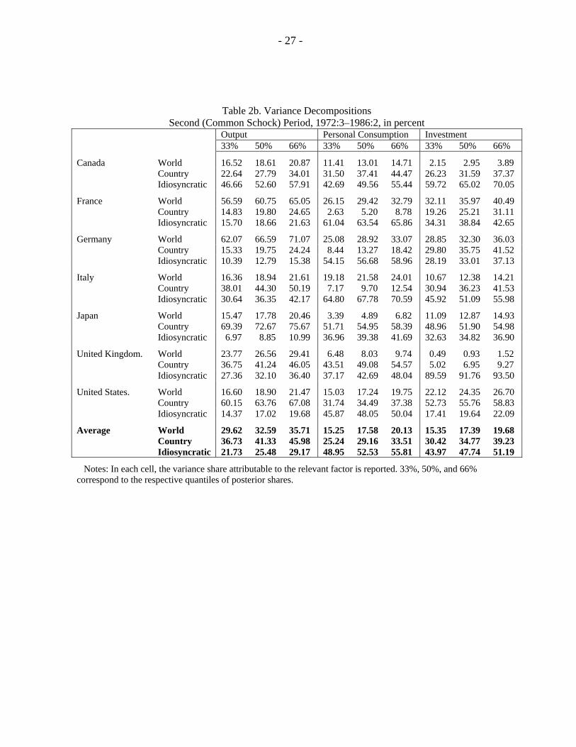
In addition to the factor estimates, for each sub-period we calculate variance decompositions that characterize the fraction of variance of each macroeconomic aggregate that is attributable to the G-7 factor, the country factor or the idiosyncratic component. The results of the variance decompositions are reported in table 2 and figures 3a-3d. Figure 3a presents the average variance of each aggregate explained by the G-7 factor. The importance of the G-7 factor is larger during the common shock period than in the first period. Not surprisingly, the G-7 factor accounts for a smaller fraction of the variance of output and consumption during the period of globalization than it does during the common shock period. These results are consistent with the findings of some recent studies documenting that there has been a decrease in the degree of business cycle synchronization from the common shock period to the globalization period (see Heathcote and Perri (2004)), Helbling and Bayoumi (2003), Monfort, Renne, Ruffer, and Vitale (2003), and Stock and Watson (2003)). For investment, though, the G-7 factor becomes more important over time.

To isolate the role of globalization in driving the degree of comovement, we compare the period of globalization with the Bretton Woods period. The average variance due to the G-7 factor has increased from roughly 7 percent in the first period to almost 25 percent in the globalization period. We also find that the average variance of consumption explained by the G-7 factor in the globalization period is almost doubled and the average share of investment variance due to the G-7 factor is roughly tripled during the globalization period relative to the first period. These findings suggest that the degree of comovement of business cycles of major macroeconomic aggregates across the G-7 countries has indeed increased during the globalization period.18

Figure 3b presents the variance of output explained by the G-7 factor for each country. For all countries, there is a significant increase in the variance of output explained by the G-7 factor in the common shock period relative to the first period. However, moving from the

18 To check the sensitivity of our results, we run additional simulations with some alternative dates for the start of globalization period. The results of these simulations indicate that our findings are quite robust to the changes in the start date of the globalization period.

- 15 -

common shock period to the globalization period, the variance explained by the G-7 factor has declined in all countries except France and Italy. While the decline in the importance of the G-7 factor from the common shock period to the globalization period is quite dramatic for Germany and Japan, it is much more modest for Canada, the United States, and the United Kingdom. More importantly, for all countries, the G-7 factor is more important in the globalization period than in the first period.

How can we explain the increase in the importance of the G-7 factor from the common shock period to the globalization period in explaining output volatility in France and Italy? A possible explanation for this result is that, while other G-7 countries liberalized their capital accounts in the 1970s (Canada, Germany, United States) or the early 1980s (Japan, United Kingdom), France and Italy did not remove all of the barriers on capital account transactions until the beginning of the 1990s. In other words, the effect of the financial integration was felt early on during the common shock period in all countries of the G-7 except Italy and France, where the full impact of financial reforms occurred only during the globalization period.19

The increase in the importance of the G-7 factor from the first period to the globalization period in explaining the volatility of output in Germany and Japan is relatively modest. To gain insight into the behavior of business cycles in Germany and Japan during the period of globalization, note that the Japanese economy suffered a prolonged recession that was aggravated by a sharp fall in asset prices and a severe banking crisis, while in the context of the unification process and the Maastricht criteria, Germany implemented a set of tight fiscal and monetary policies that contributed to a relatively long period of slow growth during the 1990s. In other words, business cycles in these countries have been less affected by the international forces than domestic ones during the period of globalization.

Figure 3c reports the variance of consumption explained by the G-7 factor in each country. To assess the impact of increased financial linkages on the degree of comovement in consumption fluctuations over time, we again focus on the first period and the period of globalization. In the majority of the cases, there has been a substantial increase in the variance of consumption due to the G-7 factor in the globalization period relative to the first period. This result is consistent with the predictions of economic theory. For example, Cole (1993) presents a model in which increased financial integration reduces the impact of wealth effects associated with a country’s own productivity shocks while it increases the wealth effects of productivity shocks abroad. These changes increase the cross-country consumption correlations. Increasing financial linkages could also increase the degree of consumption comovement as they stimulate specialization of production through the reallocation of capital in a manner consistent with countries’ comparative advantage in the production of different goods.

19 For a detailed discussion about the history of the liberalization of capital account in the G-7 countries, see Bakker and Chapple (2002).

- 16 -

Figure 3d displays the findings concerning the dynamics of investment. The variance of investment captured by the G-7 factor has increased in all countries but Japan during the period of globalization relative to the first period. In France and Italy, the share of investment variance due to the G-7 factor has risen substantially in the globalization period relative to the earlier periods. This finding is consistent with our earlier explanation that the full impact of financial reforms in Italy and France took place only during the globalization period. As noted above, the average share of investment variance due to the G-7 factor is roughly tripled during the globalization period relative to the first period. It is hard to reconcile this finding with economic theory. For example, in stochastic dynamic business cycle models, increased trade and financial linkages generally lead to lower investment correlations across countries because reductions in restrictions on capital and current account transactions induce more “resource shifting”, through which capital and other resources rapidly move to the countries receiving more favorable technology shocks (see Backus, Kehoe, and Kydland (1995) and Heathcote and Perri (2002)).

We also find that the country factor, on average, becomes less important in explaining the variance of the main macroeconomic aggregates in the globalization period relative to the first period. For example, the variance of output explained by the country factor decreased from roughly 65 percent in the first period to 43 percent in the globalization period.

V. SOURCES OF CHANGES IN THE G-7 BUSINESS CYCLES

In the previous section, we documented how the importance of the G-7 factor in explaining business cycle variation has changed over time and suggested that increased trade and financial linkages could have played an important role in explaining the observed changes. Of course, other more easily identifiable phenomena may also help explain these developments. To address this issue, we combine our dynamic factor model with a VAR and study the interrelationship between those variables thought to cause fluctuations (e.g. monetary and fiscal policy shocks) and our measures of common economic activity.20

Our econometric model follows the work of Bernanke, Bovin, and Eliasz (2002) who developed the factor-augmented VAR (FAVAR) to study the affects of monetary policy in a closed economy framework. Their work is motivated by the curse of dimensionality associated with standard VAR models: the number of parameters grows with the square of the dimension of the VAR. Our motivation is similar; with 7 countries, 3 measures of economic activity and 5 measures of potential sources of economic activity (monetary policy, fiscal policy, terms of trade, Solow residuals and oil prices), we have a system of 56 variables. With the small samples we are interested in, we would quickly exhaust degrees of freedom in a standard VAR. The FAVAR achieves parameter reduction while still incorporating essential information in the estimation procedure. In the closed economy

20 In related research, Gregory and Head (1999) and Glick and Rogoff (1995) analyze the importance of common technology and fiscal policy shocks in explaining current account dynamics.

- 17 -

framework, Bernanke, Bovin, and Eliasz (2002) find that this additional information alleviates price and liquidity puzzles traditionally found in studies using monetary VARs.

Here we are using the FAVAR not to bring additional information into the system to identify the effects of a monetary policy shock as in Bernanke et al, but to investigate the effects of a shock on world economic activity represented by the G-7 factor. That is, we are interested in the response of the G-7 factor to a shock to policy variables. An important issue in implementing this method is the choice of policy or source variables to include in the VAR. One approach would be to extract common factors from the source variables in each country and interpret the common factor as common world policy. For example, one could extract a common interest rate factor from overnight interest rates in the G-7 and use this factor as a measure of monetary policy in the VAR. However, it is difficult to interpret such a factor as a common policy. In addition, some countries differ in their choice of monetary policy instrument making it difficult to defend the selection of overnight interest rates for all countries. We choose instead to use policy or source variables in each country in the VAR.

While we report a full set of results for all countries, we focus most of our discussion on the United States because the important role played by the United States economy in driving international business cycles. For example, we analyze the importance of the U.S. based fiscal and monetary policy shocks in affecting the global economy through their impact on the G-7 factor. We also examine how oil price, terms of trade, and technology shocks affect global volatility and comovement by studying whether these shocks Granger-cause the G-7 factor. Of course, our identification scheme cannot provide the final answer on the sources of global comovement, but it adds valuable new evidence on the role of shocks originating in the dominant economy in the world.

A. The Model

Due to the short time series length of our subsamples we focus our analysis on a sequence of bi-variate VARs. Let Ft be a vector containing the G-7 factor, and St be a vector with either the country factor, interest rates, government spending, oil prices, terms of trade or Solow residuals.21 Each bi-variate VAR is then :

(6) t1t

1t

t

t

SF

)L(D)L(C)L(A)L(

SF

Ε+⎥⎦

⎤⎢⎣

⎡⎥⎦

⎤⎢⎣

⎡Φ=⎥

⎦

⎤⎢⎣

⎡

−

−

The reported results are based on a VAR with 4 lags of each variable. The results are generally robust to this choice.

21 The data for these series are from the OECD Quarterly National Accounts and IFS. Details about the definitions and sources of the data, and construction of policy measures are available upon request.

- 18 -

B. Results of Granger Causality Tests

Granger-causality tests allow us to examine the interrelationships between our estimated factors and the underlying source variables. Specifically, these tests enable us to determine which source variables help predict the factors, and whether the factors help predict the “source” variables, in which case they are perhaps not so much source as consequence. Panel A of Table 3 contains the results for the full sample period. The tests reveal that the United States does in fact appear to be a central force in the world economy. The U.S. country factor Granger causes the G-7 factor and vice versa, indicating bi-directional feedback.22 It also appears that the U.S. technology, as measured by the Solow residual, Granger causes the world factor. In fact Solow residuals constructed using the data of five countries (the United States, Canada, France, Italy, the United Kingdom) Granger cause the G-7 factor, suggesting that this technology could be common to the world. Not surprisingly, oil prices also have significant predictive power for the G-7 factor (at the 10% significance level in five countries, including France, Germany, Italy, Japan, and the United Kingdom). We now turn to the analysis of how these relationships may have evolved over time.

In Panel B, we repeat the Granger tests for the 1960:2–1972:2 subsample. Unlike in the full sample, the U.S. country factor no longer appears to drive the world economy. Moreover, the U.S. factor does not Granger cause the G-7 factor though US interest rates do. We conclude that the causal or predictive relationship from the United States to the world is relatively weak in this period. However, there is evidence that the Solow residuals in Germany and Japan are Granger causing the world cycle (G-7 factor) during this period.

Next, we turn to the common shock period, 1972:3–1986:2. In Panel C, we see that the Granger causal relationships are much stronger during this period. For example, there are strong relationships between U.S. interest rates and the world factor (interest rates in France, Germany, Japan, and the United Kingdom Granger cause the world factor as well). Additionally, there is a strong casual relationship between oil prices and the world factor. In the case of oil prices, feedback goes both ways because the world factor helps predict oil prices as well. Given the common nature of oil prices, it is not surprising that this relationship holds across all countries. We conclude that the strong comovement in this period is due to common shocks associated with sharp fluctuations in oil prices, and changes in interest rates which could be capturing the highly synchronized contractionary monetary policies during this period. Interestingly, in this period the causal relationship between Solow residuals and the world cycle (the G-7 factor) appears to be relatively weak. Moreover, there is no causal relationship between U.S. economic activity (as measured by the U.S. country factor) and the G-7 factor.

22 When we refer to VARs using the world or country factor, we are using the median of the estimated factors. Since the quantiles of the factor estimates are tight and the correlation between the median quantile and say the 5% or 95% quantiles are very close to 1, uncertainty in the factor estimates should have minimal impact on the results.

- 19 -

In the final period (Table 3d), the link between the U.S policy variables and the world economy tends to disappear. For example, the domestic interest rates, measured by the Fed Funds rate, no longer Granger causes the G-7 factor as they did in the previous periods. Unlike in the full sample period, the U.S. country factor does not help predict the G-7 factor during the period of globalization. Moreover, the predictive power in technology shocks flows from the world to the United States as the G-7 factor seems to help predict the U.S. Solow residual, but not vice versa. We interpret these results as indicating that while the United States can still “export” its policy shocks to the rest of the world, there are stronger international linkages through which the rest of the world appears to have a larger effect on economic activity in the United States, and, in fact, the results suggest that the global (G-7) factor helps predict fluctuations in the U.S. country factor in this period.

How are these results related to our findings in the previous section? The results in this section are consistent with the temporal changes in variance decompositions we reported earlier. In particular, we document that there is an increase in the variance of the U.S. output due to the G-7 factor implying that that the global factors play a larger role in explaining the volatility of U.S. output in the globalization period than the first period (and the full period). The results of this section suggest that while the link between the U.S. economy and the G-7 factor is strong for the entire sample, the G-7 factor Granger causes the U.S. factor in the globalization period suggesting that global forces become more influential in predicting the economic activity in the United States over time.23

VI. SUMMARY AND CONCLUSION

We study the changes in the nature of G-7 business cycles over time by estimating common dynamic components in the main macroeconomic aggregates (output, consumption, and investment). In particular, we employ a Bayesian dynamic latent factor model and decompose macroeconomic fluctuations in these variables into the following: (i) the G-7 factor (common across all variables/countries); (ii) country factors (common across aggregates in a country); and (iii) factors specific to each variable.

We first show that to the extent that there are country-specific and worldwide sources of economic shocks, these play different roles at different points in time and around the globe. In some episodes, the country factor is more strongly reflective of domestic economic activity, while in others the domestic growth reflects the common pattern embodied in the

23 One potential explanation of these findings could be the rapid increase in trade and financial flows between the United Stares and the rest of world. For example, the average growth in international trade, measured by the sum of exports and imports, has been more than two times larger than that of output in the United States. Moreover, there has been a major change in the composition of trade flows as the share of trade based on vertical specialization and trade of intermediate goods in total U.S. trade has registered a significant increase during the period of globalization. Additionally, as we noted in the introduction, there has been a dramatic increase in the U.S. holdings of foreign assets during the globalization period.

- 20 -

G-7 factor. We document that the G-7 factor is able to explain a sizeable fraction of volatility of the three aggregates for the period 1960:1–2003:4. In particular, the G-7 factor on average accounts for more than 26 percent of output variation and it explains roughly 16 and 19 percent the volatility of consumption and investment, respectively. We also find that the importance of the G-7 factor differs quite a bit across countries.

We then examine the evolution of the roles played by the G-7 and country-specific factors in driving business cycles in three distinct sub-periods. Our results suggest that the G-7 factor accounts for a smaller fraction of variance of output and consumption during the period of globalization than it does during the common shock period. More importantly, there is a marked increase in the variance of output due to the G-7 factor from the first period to the globalization period. In addition, the G-7 factor, on average, explains a substantially larger fraction of consumption and investment volatility in the globalization period than it does in the first period. These findings indicate that the degree of comovement of business cycles of major macroeconomic aggregates across the G-7 countries has indeed increased during the globalization period.

Increased global linkages also affect the dynamics of comovement by changing the nature and frequency of shocks. We also study the evolution of the roles played by different types of shocks in explaining the synchronization of business cycles over time. We combine our estimated dynamic factors with variables thought to have a causal or predictive relationship with the G-7 factor in a series of bi-variate vector autoregression. This allows us to study the interrelationship between those variables thought to cause fluctuations and our measures of common economic activity. Our findings indicate that the period labeled the “common shock” period is indeed driven by common shocks associated with the fluctuations in oil prices. In the globalization period, the world seems to evolved to a stage where the United States follows the lead of the world economy rather than vice versa.

- 21 -

REFERENCES Ahmed, S., B.W. Ickes, P. Wang, and B.S. Yoo, 1993, “International Business Cycles,”

American Economic Review, Vol. 83, pp. 335–59.

Andrews, Donald, 1993, “Tests for Parameter Instability and Structural Change with Unknown Change Point,” Econometrica, Vol. 61, pp. 821–56.

Artis, M., 2003, “Is There a European Business Cycle?” CESIFO Working Paper No. 1053 (Munich: CESIFO’s parent org.)

Backus D.K., P.J. Kehoe, and F.E. Kydland, 1995, “International Business Cycles: Theory and Evidence,” Frontiers of Business Cycle Research, ed. by C. Plosser (Princeton University Press), pp. 331–57.

Bakker, A., and B. Chapple, 2002, “Advanced Country Experiences with Capital Account Liberalization,” IMF Occasional Paper No. 214 (Washington: International Monetary Fund).

Baxter, M., 1991, “Business Cycles, Stylized Facts, and The Exchange Rate Regime: Evidence from The United States,” Journal of International Money and Finance, Vol. 10, pp. 71–88.

———, and A.C. Stockman, 1989, “Business Cycles and The Exchange Rate Regime: Some International Evidence,” Journal of Monetary Economics, Vol. 23, pp. 377–400.

———, and M. Kouparitsas, 2004, “Determinants of Business Cycle Comovement: A Robust Analysis,” NBER Working Paper No. 10725, (Cambridge: Massachusetts)

Bernanke, B.S., J. Boivin, and P. Eliasz, 2002, “Measuring the Effects of Monetary Policy Shocks: A Factor-Augmented Vector Autoregressive (FAVAR) Approach,” Working Paper, Princeton University.

Blanchard, O., and J. Simon, 2001, “The Long and Large Decline in U.S. Output Volatility,” Brookings Papers in Economic Activity, pp. 135–174.

Bronfenbrenner, M., 1969, Is the Business Cycle Obsolete? (New York: Wiley-Interscience).

Canova, Fabio, Matteo Ciccarelli, and Eva Ortega, 2003, “Similarities and Convergence in G-7 Cycles,” Working Paper, University of Pompeu Fabra.

Carter, C.K., and R. Kohn, 1994, “On Gibbs Sampling for State Space Models,” Biometrika, Vol. 81, pp. 541–53.

Chib, Siddhartha, and Edward Greenberg, 1996, “Markov Chain Monte Carlo Simulation Methods in Econometrics,” Econometric Theory, Vol. 12, pp. 409–31.

- 22 -

Christodulakis, N., S.P. Dimelis, and T. Kollintzas, 1995, “Comparisons of Business Cycles in The EC: Idiosyncracies and Regularities,” Economica, Vol. 62, pp. 1–27.

Clark, Todd E., and van Wincoop, Eric, 2001, “Borders and Business Cycles,” Journal of International Economics, Vol. 55, pp. 59–85.

Cole, H., 1993, “The Macroeconomic Effects of World Trade in Financial Assets,” Federal Reserve Bank of Minneapolis, Quarterly Review, Vol. 17, pp. 12–21.

Doyle, B., and J. Faust, 2003, “Breaks in the Variability and Comovement of G-7 Economic Growth,” Working Paper, Federal Reserve Board.

Frankel, Jeffrey A., and Rose, Andrew K, 1998, “The Endogeneity of the Optimum Currency Area Criteria,” Economic Journal, Vol. 108, pp. 1009–25.

Forni, M., and L. Reichlin, 2001, “Federal Policies and Local Economies: Europe and the U.S.,” European Economic Review, Vol. 45, pp. 109–34.

Forni, M., M. Hallin, M. Lippi, and L. Reichlin, 2002, “The Generalized Dynamic Factor Model: Identification and Estimation,” Review of Economics and Statistics, Vol. 82, pp. 540–54.

Gerlach, S., 1988, “World Business Cycles Under Fixed and Flexible Exchange Rates,” Journal of Money, Credit, and Banking,” Vol. 20, pp. 621–32.

Geweke, John, 1996, “Monte Carlo Simulation and Numerical Integration,” in Handbook of Computational Economics, ed. by H. Amman, D. Kendrick and J. Rust (Amsterdam: North-Holland), pp. 731–800.

———, 1997, “Posterior Simulators in Econometrics,” Advances in Economics and Econometrics: Theory and Applications, Vol. III, ed. by D. Kreps and K.F. Wallis (Cambridge: Cambridge University Press), pp. 128–65.

Glick, Reuven, and Kenneth Rogoff, 1995, “Global Versus Country-Specific Productivity Shocks and the Current Account,” Journal of Monetary Economics, Vol. 35, pp. 159–192.

Gregory, A. W., A. C. Head, and J. Raynauld, 1997, “Measuring World Business Cycles,” International Economic Review, Vol. 38, pp. 677–702.

Gregory, A. W., and A. C. Head, 1999, “Common and Country-Specific Fluctuations in Productivity, Investment, and The Current Account,” Journal of Monetary Economics, Vol. 44, pp. 423–51.

Heathcote, Jonathan, and Fabrizio Perri, 2002, “Financial Autarky and International Business Cycles,” Journal of Monetary Economics, Vol. 49, pp. 601–28.

- 23 -

———, 2004, “Financial Globalization and Real Regionalization,” Journal of Economic Theory, Vol. 119/1, pp. 184–206.

Helbling, T., and T. Bayoumi, 2002, “G-7 Business Cycle Linkages Revisited,” IMF Working Paper (Washington: International Monetary Fund).

Hirata, H., 2003, “The Role of Energy Prices in The Japanese Business Cycles,” Working Paper, Brandeis University.

Imbs, J., 2004a, “Trade, Finance, Specialization and Synchronization,” forthcoming in Review of Economics and Statistics.

———, 2004b, “Real Effects of Financial Integration,” forthcoming in IMF Staff Papers (Washington: International Monetary Fund).

International Monetary Fund, 2002, World Economic Outlook, September, pp. 104–37.

Kalemli-Ozcan, S., B. Sorensen, and O. Yosha, 2003, “Risk Sharing and Industrial Specialization: Regional and International Evidence,” American Economic Review, Vol. 93, pp. 903–18.

Kose, M. A., C. Otrok, and C. Whiteman, 2003, “International Business Cycles: World, Region, and Country Specific Factors,” American Economic Review, Vol. 93, pp. 1216–39.

Kose, M. A., E. S. Prasad, and M. Terrones, 2003, “How Does Globalization Affect the Synchronization of Business Cycles?” American Economic Review-Papers and Proceedings, Vol. 93, pp. 57–62.

Kose, M. A., and K. Yi, 2005, “Can the Standard International Business Cycle Model Explain the Relation between Trade and Comovement?,” forthcoming, Journal of International Economics.

Lane, Philip and Gian Maria Milesi-Ferretti, 2001, “The External Wealth of Nations: Estimates of Foreign Assets and Liabilities for Industrial and Developing Countries,” Journal of International Economics, Vol. 55, pp. 263–94.

———, 2003, “International Financial Integration,” IMF Staff Papers (Washington: International Monetary Fund), Vol. 50, pp. 82–113.

Lumsdaine, R. L., and E. S. Prasad, 2003, “Identifying the Common Component in International Economic Fluctuations,” Economic Journal, No. 48, pp. 101–27.

McConnell, M. and G. Perez-Quiros, 2000, “Output Fluctuations in The United States: What Has Changed Since the Early 1980s?,” American Economic Review, Vol. 90, pp. 1464–76.

- 24 -

Monfort, A., J. R. Renne, R. Rufle, and G. Vitale, 2003, “Is Economic Activity in The G-7 Synchronized? Common Shocks vs. Spillover Effects,” Working Paper, European Central Bank.

Obstfeld, Maurice, and Kenneth Rogoff, 2002. “Global Implications of Self-Oriented National Monetary Rules,” Quarterly Journal of Economics, Vol. 177, pp. 503–35.

Otrok, C. and C. H. Whiteman, 1998, “Bayesian Leading Indicators: Measuring and Predicting Economic Conditions in Iowa,” International Economic Review, Vol 39:4.

Otto, Glenn; Voss, Graham, and Luke Willard, 2003, “Understanding OECD Output Correlations,” Working Paper, University of New South Wales.

Sargent, Thomas J., and Christopher A. Sims, 1977, “Business Cycle Modeling Without Pretending to Have Too Much A Priori Economic Theory,” in Christopher A. Sims et al., New Methods in Business Cycle Research, (Minneapolis: Federal Reserve Bank of Minneapolis).

Smith, P.A., and P.M. Summers, 2002, “On the Interactions Between Growth and Volatility in A Markov Switching Model of GDP,” Working Paper, The University of Melbourne.

Stock, James H., and Mark W. Watson, 1989, “New Indexes of Coincident and Leading Economic Indicators,” NBEResearch, Macroeconomics Annual 1989, (Cambridge: The MIT Press), pp. 351–94.

———, 1992, “A Procedure for Predicting Recessions with Leading Indicators: Econometric Issues and Recent Performance,” Federal Reserve Bank of Chicago Working Paper No. 92-7, (Chicago: Federal Reserve Bank of Chicago).

———, 1993, “A Procedure for Predicting Recessions with Leading Indicators: Econometric Issues and Recent Experience,” Business Cycles, Indicators, and Forecasting, ed. by James H. Stock and Mark W. Watson (Chicago: The University of Chicago Press), pp. 95–153.

———, 2002, “Has The Business Cycle Changed and Why?” NBEResearch, Macroeconomics Annual (Cambridge: Massachuttes).

———, 2003, “Understanding Changes in International Business Cycles,” NBER Working Paper No. 9859 (Cambridge: Massachuttes).

Tanner, M., and W. H. Wong, 1987, “The Calculation of Posterior Distributions by Data Augmentation,” Journal of the American Statistical Association, Vol. 82, pp. 84–88.

- 25 -

Table 1. Variance Decompositions

Full Period, 1960:1–2003:4, in percent Output Personal Consumption Investment 33% 50% 66% 33% 50% 66% 33% 50% 66%

Canada World 12.34 13.67 15.14 5.67 6.57 7.50 4.32 5.05 5.80 Country 35.03 38.95 43.24 38.86 43.24 47.64 17.24 19.54 22.00 Idiosyncratic 42.89 47.23 51.13 45.65 50.10 54.35 73.07 75.26 77.41

France World 56.12 58.76 61.64 34.47 37.34 40.09 42.37 45.03 47.77 Country 20.58 24.07 27.56 4.52 6.87 9.63 20.41 23.67 27.06 Idiosyncratic 14.90 16.79 18.82 53.49 54.97 56.42 29.37 31.41 33.26

Germany World 29.83 31.94 34.10 17.37 18.99 20.63 20.64 22.46 24.24 Country 41.94 44.83 47.65 15.88 17.91 20.02 36.86 39.52 42.23 Idiosyncratic 20.99 23.05 25.09 61.41 62.91 64.38 36.03 37.95 39.84

Italy World 22.64 24.34 26.02 18.12 19.96 21.77 9.43 10.59 11.80 Country 44.96 47.73 50.48 24.44 26.61 28.87 45.18 47.91 50.67 Idiosyncratic 25.52 27.82 30.16 51.50 53.25 55.00 38.91 41.38 43.83

Japan World 28.92 30.84 32.87 14.29 15.82 17.43 24.35 26.15 28.06 Country 60.09 62.27 64.32 45.83 47.78 49.70 42.17 44.20 46.20 Idiosyncratic 5.44 6.52 7.72 35.20 36.31 37.34 28.62 29.46 30.33

United Kingdom World 16.81 18.26 19.73 4.12 4.87 5.67 11.38 12.64 13.93 Country 48.56 52.07 55.90 48.50 52.03 55.98 8.48 9.74 11.07 Idiosyncratic 25.76 29.42 32.87 39.21 43.01 46.46 76.09 77.39 78.62

United States. World 8.11 9.24 10.45 6.07 6.98 7.97 8.93 10.12 11.43 Country 69.62 72.40 75.01 40.38 42.10 43.93 48.86 50.82 52.75 Idiosyncratic 15.70 18.11 20.63 49.09 50.85 52.36 37.29 38.95 40.54

Average World 24.97 26.72 28.56 14.30 15.79 17.29 17.35 18.86 20.43 Country 45.83 48.90 52.02 31.20 33.79 36.54 31.31 33.63 35.99 Idiosyncratic 21.60 24.13 26.63 47.94 50.20 52.33 45.63 47.40 49.12

Notes: In each cell, the variance share attributable to the relevant factor is reported. 33%, 50%, and 66% correspond to the respective quantiles of posterior shares.

- 26 -

Table 2a. Variance Decompositions

First (BW) Period, 1960:1–1972:2, in percent Output Personal Consumption Investment 33% 50% 66% 33% 50% 66% 33% 50% 66%






United Kingdom. World 1.51 4.29 9.98 0.45 1.09 2.30 3.89 10.33 25.02 Country 59.55 66.31 72.34 41.20 45.53 50.31 28.90 37.38 43.71 Idiosyncratic 21.36 26.07 30.62 47.42 52.15 56.35 41.69 46.30 50.69




- 27 -

Table 2b. Variance Decompositions

Second (Common Schock) Period, 1972:3–1986:2, in percent Output Personal Consumption Investment 33% 50% 66% 33% 50% 66% 33% 50% 66%










- 28 -

Table 2c. Variance Decompositions

Third (Globalization) Period, 1986:3–2003:4, in percent Output Personal Consumption Investment 33% 50% 66% 33% 50% 66% 33% 50% 66%










- 29 -

Table 3. Granger Causality Tests for the G-7 Factor

Canada France Germany Italy Japan United Kingdom.

United States

Source S⇒F S⇐F S⇒F S⇐F S⇒F S⇐F S⇒F S⇐F S⇒F S⇐F S⇒F S⇐F S⇒F S⇐F

Panel A Country Factor 5.15 3.05 1.61 3.78 0.60 1.47 3.85 6.66 1.47 3.11 2.28 0.99 3.40 2.98 Full Government Spend 2.15 3.23 1.39 0.79 0.80 2.84 2.16 1.45 2.64 3.01 1.18 0.77 1.68 1.13 Sample Interest Rate 1.81 1.45 1.83 1.08 5.38 2.40 2.55 0.15 4.04 4.85 2.43 1.78 1.93 0.75 Oil 1.73 1.56 2.23 2.06 2.07 1.80 2.10 1.58 2.13 1.43 2.35 1.71 1.73 1.53 Solow Residuals 4.80 2.64 3.08 2.05 1.53 6.03 4.42 1.37 1.36 2.36 3.71 1.41 3.87 1.03 TOT 0.35 0.18 3.98 3.74 0.80 0.93 2.32 1.37 1.70 0.13 2.50 0.80 1.71 1.02

Panel B Country Factor 1.23 0.71 2.06 2.00 1.37 0.87 2.93 0.76 1.98 0.34 1.09 0.97 0.56 2.85 First Government Spend 0.92 2.61 1.24 0.84 1.25 1.33 0.06 6.16 0.68 0.51 2.19 2.00 1.02 0.62 Period Interest Rate 2.01 1.67 1.09 1.67 0.83 1.85 0.73 0.28 2.81 1.03 0.57 1.41 2.99 2.39 Oil 4.35 1.13 0.41 0.83 0.37 1.34 0.10 1.53 0.80 0.32 1.29 1.14 2.16 0.38 Solow Residuals 0.91 1.19 0.84 1.38 4.56 0.67 0.84 0.33 3.53 1.21 0.28 1.29 0.17 0.96 TOT 0.35 1.17 0.16 0.65 0.47 1.00 1.01 2.61 0.66 1.45 2.63 1.53 0.24 0.48

Panel C Country Factor 1.72 2.06 1.54 0.90 1.38 0.86 8.04 4.15 0.93 0.69 1.12 0.84 1.60 1.67 Second Government Spend 1.66 1.61 0.36 1.16 0.86 3.42 1.22 0.64 2.63 4.77 1.02 0.67 1.32 0.50 Period Interest Rate 1.77 0.29 4.36 0.38 3.87 0.35 1.81 1.35 2.67 2.12 3.20 0.70 4.39 0.44 Oil 2.45 5.46 3.61 4.83 3.26 4.47 3.24 4.30 3.06 3.83 3.09 4.00 2.62 5.04 Solow Residuals 1.54 1.16 0.76 1.41 2.70 0.36 5.30 5.64 0.39 0.48 0.78 0.74 1.05 1.06 TOT 1.94 1.86 3.70 4.42 1.51 2.18 3.43 3.14 1.66 1.03 1.29 1.03 2.72 1.68

Panel D Country Factor 3.41 0.98 2.65 1.30 0.76 1.37 1.37 1.64 1.89 0.23 2.77 2.10 1.81 2.88 Third Government Spend 0.57 1.90 2.80 0.73 1.52 0.37 0.42 0.22 1.92 1.22 0.36 0.72 0.35 0.53 Period Interest Rate 0.79 3.89 0.65 1.80 1.70 1.37 1.75 0.83 0.79 1.43 1.08 2.03 0.79 2.02 Oil 0.18 0.52 0.34 0.51 0.38 0.53 0.25 0.40 0.28 0.78 0.17 0.32 0.10 0.62 Solow Residuals 1.79 3.05 3.92 3.35 1.20 2.58 0.26 0.42 1.58 1.30 2.15 5.16 1.21 2.97 TOT 0.79 0.19 0.31 1.52 0.67 1.25 0.78 1.10 0.10 0.97 0.55 2.02 0.36 0.58

Notes: S⇒F indicates a Granger test that the listed source variable Granger causes the world factor. S⇐F indicates a test for reverse causality. The test statistic is a F-statistic distributed F(4,162) F(4,36), F(4,43), and F(4,57) in the 4 samples. The statistics in bold, italics, and underlined indicate statistical significance at the 1 percent, 5 percent, and 10 percent levels, respectively.

- 30 -

Figure 1a.

Notes: Solid line=G-7 factor; dotted line= 5 and 95 % quantile bands.

Figure 1b.

Notes: Solid line=G-7 factor; dotted line=country factor; dashed line= output

G-7 Factor and U.S. Country Factor

-3.00

-2.00

-1.00

0.00

1.00

2.00

3.00

4.00

5.00

1960

Q2

1962

Q2

1964

Q2

1966

Q2

1968

Q2

1970

Q2

1972

Q2

1974

Q2

1976

Q2

1978

Q2

1980

Q2

1982

Q2

1984

Q2

1986

Q2

1988

Q2

1990

Q2

1992

Q2

1994

Q2

1996

Q2

1998

Q2

2000

Q2

2002

Q2

Years

Gro

wth

Rat

e (%

)

G-7 Factor

-4.00

-3.00

-2.00

-1.00

0.00

1.00

2.00

3.00

4.0019

60Q

2

1962

Q2

1964

Q2

1966

Q2

1968

Q2

1970

Q2

1972

Q2

1974

Q2

1976

Q2

1978

Q2

1980

Q2

1982

Q2

1984

Q2

1986

Q2

1988

Q2

1990

Q2

1992

Q2

1994

Q2

1996

Q2

1998

Q2

2000

Q2

2002

Q2

Years

Gro

wth

Rat

e (%

)

- 31 -

Figure 1c.


Figure 1d.


G-7 Factor and Japan Country Factor

-4.00

-2.00

0.00

2.00

4.00

6.00

8.00

1960

Q2

1962

Q2

1964

Q2

1966

Q2

1968

Q2

1970

Q2

1972

Q2

1974

Q2

1976

Q2

1978

Q2

1980

Q2

1982

Q2

1984

Q2

1986

Q2

1988

Q2

1990

Q2

1992

Q2

1994

Q2

1996

Q2

1998

Q2

2000

Q2

2002

Q2

Years

Gro

wth

Rat

e (%

)

G-7 Factor and German Country Factor

-6.00

-4.00

-2.00

0.00

2.00

4.00

6.0019

60Q

2

1962

Q2

1964

Q2

1966

Q2

1968

Q2

1970

Q2

1972

Q2

1974

Q2

1976

Q2

1978

Q2

1980

Q2

1982

Q2

1984

Q2

1986

Q2

1988

Q2

1990

Q2

1992

Q2

1994

Q2

1996

Q2

1998

Q2

2000

Q2

2002

Q2

Years

Gro

wth

Rat

e (%

)

- 32 -

Figure 2.

Notes: Dark solid line=G-7 factor median (Full Sample); dashed line= G-7 factor median (1st Period); light solid line= G-7 factor median (2nd Period); dotted line= G-7 factor median (3rd Period).

G-7 Factors - Full Sample and 3 Subperiods

-4.00

-3.00

-2.00

-1.00

0.00

1.00

2.00

3.00

4.0019

60Q

2

1962

Q2

1964

Q2

1966

Q2

1968

Q2

1970

Q2

1972

Q2

1974

Q2

1976

Q2

1978

Q2

1980

Q2

1982

Q2

1984

Q2

1986

Q2

1988

Q2

1990

Q2

1992

Q2

1994

Q2

1996

Q2

1998

Q2

2000

Q2

2002

Q2

Years

Gro

wth

Rat

e (%

)

- 33 -

Figure 3a.

Average Variance Explained by the G-7 Factor (%)

0.0

5.0

10.0

15.0

20.0

25.0

30.0

35.0

Output Consumption Investment

Frac

tion

of V

aria

nce

(%)

60:1-72:2 72:3-86:2 86:3-03:4

Figure 3b.

Variance of Output Explained by the G-7 Factor (%)

0.0

10.0

20.0

30.0

40.0

50.0

60.0

70.0

80.0

Canada France Germany Italy Japan U.K. U.S.

Frac

tion

of V

aria

nce

(%)

60:1-72:2 72:3-86:2 86:3-03:4

- 34 -

Figure 3c.

Variance of Consumption Explained by the G-7 Factor (%)

0.0

5.0

10.0

15.0

20.0

25.0

30.0

35.0


Frac

tion

of V

aria

nce

(%)

60:1-72:2 72:3-86:2 86:3-03:4

Figure 3d.

Variance of Investment Explained by the World Factor (%)

0.0

10.0

20.0

30.0

40.0

50.0

60.0

70.0


Frac

tion

of V

aria

nce

(%)

60:1-72:2 72:3-86:2 86:3-03:4

understanding the evolution of world business cycles · understanding the evolution of world...

Documents