Understanding the TSL EBSD Data Collection System

With thanks to: Harry Chien, Lisa Chan, Bassem El-Dasher, Gregory Rohrer

1Last revised: 12th Apr. ‘14

27-750Texture, Microstructure & Anisotropy

A.D. Rollett

Overview• Understanding the diffraction patterns

– Source of diffraction– SEM setup per required data– The makeup of a pattern

• Setting up the data collection system– Environment variables– Phase and reflectors

• Capturing patterns– Choosing video settings – Background subtraction

• Image Processing– Detecting bands: Hough transform– Enhancing the transform: Butterfly mask– Selecting appropriate Hough settings– Origin of Image Quality (I.Q.)

2

Overview (cont’d)

• Indexing captured patterns– Identifying detected bands: Triplet method– Determining solution: Voting scheme– Origin of Confidence Index (C.I.)– Identifying a solution in multi-phase materials

• Calibration– Physical meaning– Method and need for tuning

• Scanning– Choosing appropriate parameters

• General reference on orientation mapping: “Orientation Mapping” by Anthony D Rollett & Katayun Barmak; uploaded to Box as CH11-Orientation_Mapping-final_proofs.pdf.

3

Questions (1)• Why do we need to position the specimen at the eucentric point?• Why does the specimen need to be tilted at a steep angle of incidence

(70°) to the electron beam?• Why is it so important to avoid contact between a specimen and the

phosphor screen?• What is the function of the phosphor screen?• What is the characteristic appearance of a diffraction pattern in EBSD?• Why is specimen surface preparation so important?• What are reflectors and how do you choose them?• What is the Hough Transform?• What does “binning” refer to (in connection with Hough Transforms)?• What is a “sharpening mask”?• What does “frame averaging” do for acquisition?

4

Questions (2)

• What does background subtraction do?• What is image quality?• What are the coordinates of the image after the Hough

transform has been applied?• Why is the Hough transform effective for detecting lines?• What are interzonal angles (in the context of an EBSD

diffraction pattern)?• What is the “confidence index” and how is it calculated?• Why is it important to have a flat surface for the specimen?

5

SEM Schematic Overview

• All students using this system need to know how to use SEM. It is recommended that all users take SEM courses offered by the MSE department

6

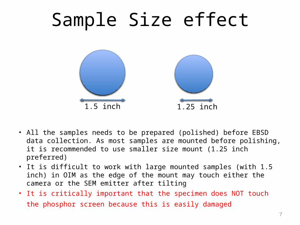
Sample Size effect

• All the samples needs to be prepared (polished) before EBSD data collection. As most samples are mounted before polishing, it is recommended to use smaller size mount (1.25 inch preferred)

• It is difficult to work with large mounted samples (with 1.5 inch) in OIM as the edge of the mount may touch either the camera or the SEM emitter after tilting

• It is critically important that the specimen does NOT touch the phosphor

screen because this is easily damaged

1.25 inch1.5 inch

7

Diffraction Pattern-Observation Events• OIM computer asks Microscope Control Computer to place a fixed

electron beam on a spot on the sample• A cone of diffracted electrons is intercepted by a specifically placed

phosphor screen• Incident electrons excite the phosphor, producing photons• A Charge Coupled Device (CCD) Camera detects and amplifies the

photons and sends the signal to the OIM computer for indexing

8

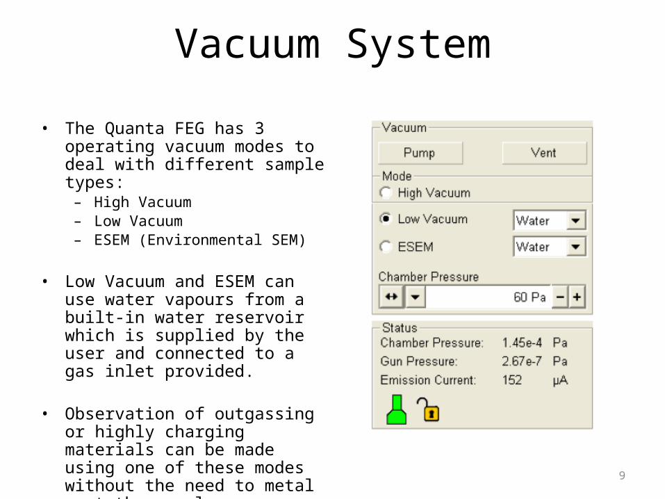
Vacuum System

• The Quanta FEG has 3 operating vacuum modes to deal with different sample types:

– High Vacuum– Low Vacuum– ESEM (Environmental SEM)

• Low Vacuum and ESEM can use water vapours from a built-in water reservoir which is supplied by the user and connected to a gas inlet provided.

• Observation of outgassing or highly charging materials can be made using one of these modes without the need to metal coat the sample.

9

Vacuum Status

• Green: PUMPED to the desired vacuum mode• Orange: TRANSITION between two vacuum modes

(pumping / venting / purging) • Grey: VENTED for sample or detector exchange

10

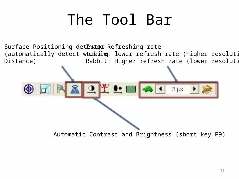
The Tool Bar

Image Refreshing rateTurtle: lower refresh rate (higher resolution)Rabbit: Higher refresh rate (lower resolution)

Automatic Contrast and Brightness (short key F9)

Surface Positioning detector (automatically detect working Distance)

11

Eucentric Position

Note that eucentric position only occurs when the working distance is 10.

12

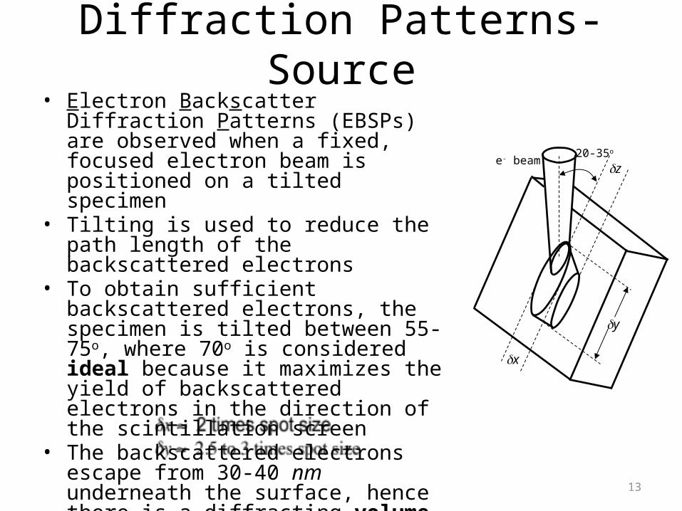
Diffraction Patterns-Source• Electron Backscatter Diffraction Patterns

(EBSPs) are observed when a fixed, focused electron beam is positioned on a tilted specimen

• Tilting is used to reduce the path length of the backscattered electrons

• To obtain sufficient backscattered electrons, the specimen is tilted between 55-75o, where 70o is considered ideal because it maximizes the yield of backscattered electrons in the direction of the scintillation screen

• The backscattered electrons escape from 30-40 nm underneath the surface, hence there is a diffracting volume

• Note that and

e- beamdz

dy

dx

20-35o

13

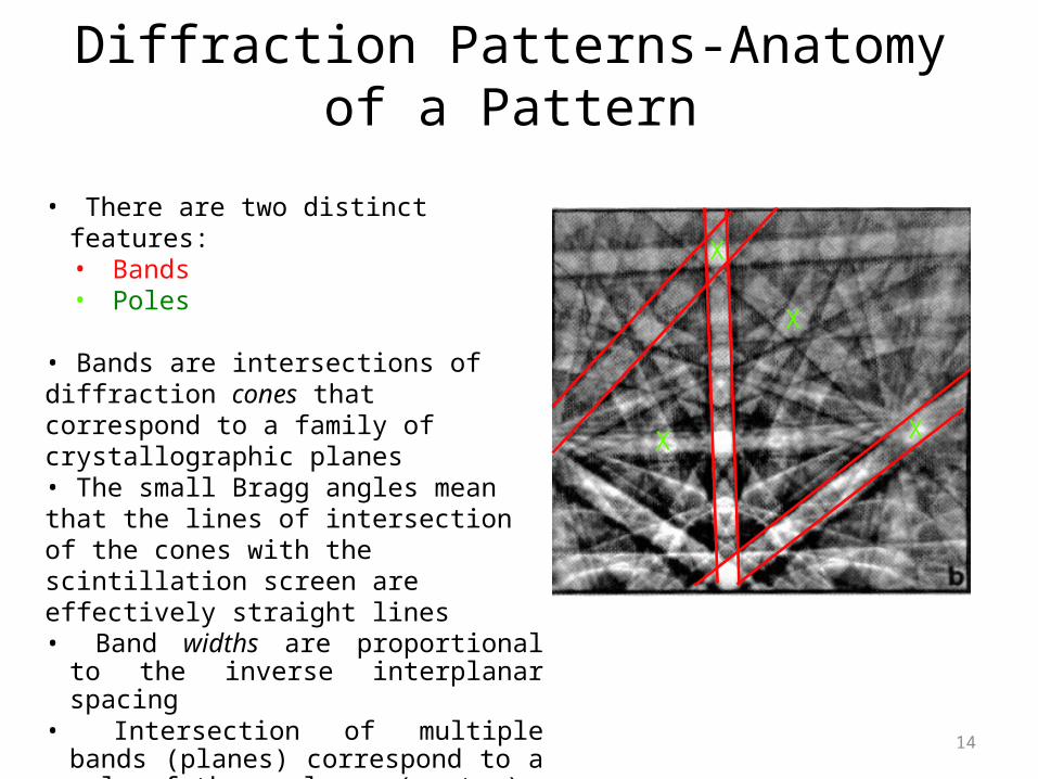
Diffraction Patterns-Anatomy of a Pattern

• There are two distinct features:• Bands• Poles

• Bands are intersections of diffraction cones that correspond to a family of crystallographic planes• The small Bragg angles mean that the lines of intersection of the cones with the scintillation screen are effectively straight lines• Band widths are proportional to the inverse

interplanar spacing • Intersection of multiple bands (planes)

correspond to a pole of those planes (vector)• Note that while the bands are bright, they

are surrounded by thin dark lines on either side

X

X

X

X

14

Diffraction Pattern-SEM Settings

• Increasing the Accelerating Voltage increases the energy of the electrons Increases the diffraction pattern intensity

• Higher Accelerating Voltage also produces narrower diffraction bands (a vs. b) and is necessary for adequate diffraction from coated samples (c vs. d)

• Larger spot sizes (beam current) may be used to increase diffraction pattern intensity

• High resolution datasets and non-conductive materials require lower voltage and spot size settings

• For insulators (most ceramics), consider using a low-vacuum “environmental” SEM.

15

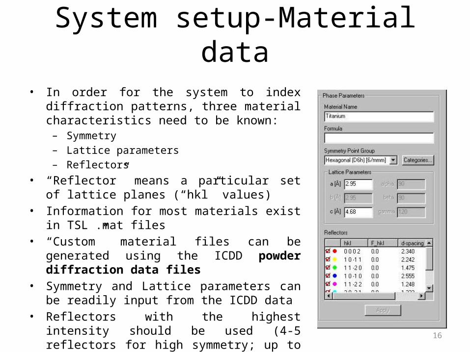
System setup-Material data

• In order for the system to index diffraction patterns, three material characteristics need to be known:

– Symmetry– Lattice parameters– Reflectors

• “Reflector” means a particular set of lattice planes (“hkl” values)

• Information for most materials exist in TSL .mat files• “Custom” material files can be generated using the

ICDD powder diffraction data files• Symmetry and Lattice parameters can be readily

input from the ICDD data• Reflectors with the highest intensity should be used

(4-5 reflectors for high symmetry; up to 12 reflectors for low symmetry)

16

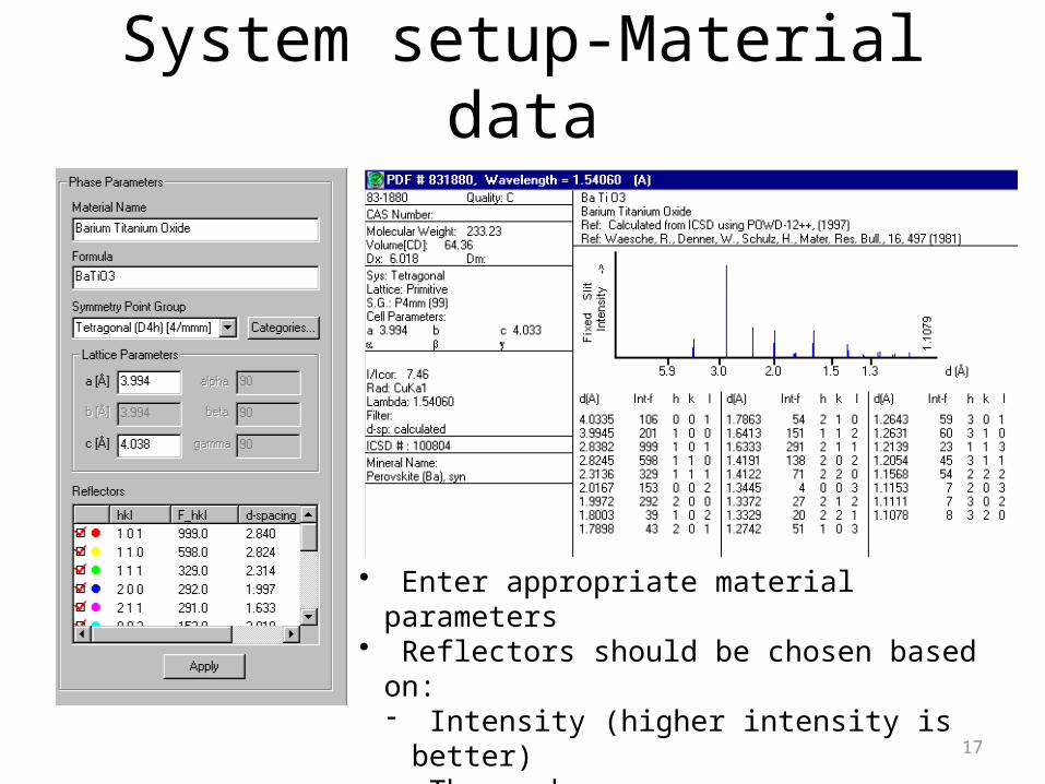
System setup-Material data

• Enter appropriate material parameters• Reflectors should be chosen based on:- Intensity (higher intensity is better)- The number per zone

17

Pattern capture-Background

Live signal Averaged signal• The background is the fixed variation in the captured frames due to the spatial variation in intensity

of the backscattered electrons• Removal is done by averaging 8 frames (SEM in TV scan mode)• Note the variation of intensity in the images. The brightest point (marked with X) should be close to

the center of the captured circle. • The location of this bright spot can be used to indicate how appropriate the Working Distance is. A

low bright spot = WD is too large and vice versa

18

Pattern capture-Background Subtraction

Without subtraction With subtraction

• The background subtraction step is critical as it “brings out” the bands in the pattern

• The “Balance” slider can be used to aid band detection. Usually a slightly lower setting improves indexing even though it may not appear better to the human eye

19

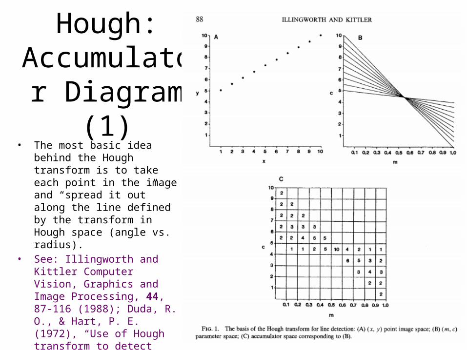
Hough: Accumulator Diagram (1)

• The most basic idea behind the Hough transform is to take each point in the image and “spread it out” along the line defined by the transform in Hough space (angle vs. radius).

• See: Illingworth and Kittler Computer Vision, Graphics and Image Processing, 44, 87-116 (1988); Duda, R. O., & Hart, P. E. (1972), “Use of Hough transform to detect lines and curves in picture”, Communications of the ACM, 15(1), 11-15.

20

Hough: Accumulator Diagram (2)• The following is quoted (12 iv 14) from:

http://www.ebsd-image.org/documentation/reference/ops/hough/op/houghtransform.html

21

“Effectively, this transformation converts each pixel of the image space into a sinusoidal curve in the Hough space. The calculated r value is rounded to the closest pixel rj. The intensity of the pixels (qj, rj) that are part of the sinusoidal curve are augmented by the intensity of the corresponding pixel (x i,yi) in the image space. The accumulation of these intensities give rise to peaks in the Hough space which corresponds to the q and r coordinates of the bands in the image space.”

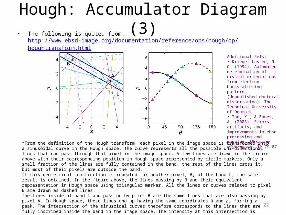
Hough: Accumulator Diagram (3)• The following is quoted from: http://www.ebsd-image.org/documentation/reference/ops/hough/op/

houghtransform.html

22

“From the definition of the Hough transform, each pixel in the image space is transformed into a sinusoidal curve in the Hough space. The curve represents all the possible uni-dimensional lines that can pass through that pixel in the image space. A few lines are drawn in the figure above with their corresponding position in Hough space represented by circle markers. Only a small fraction of the lines are fully contained in the band, the rest of the lines cross it, but most of their pixels are outside the band.If this geometrical construction is repeated for another pixel, B, of the band L, the same result is obtained. In the figure above, the lines passing by B and their equivalent representation in Hough space using triangular marker. All the lines or curves related to pixel B are drawn as dashed lines.The lines inside of band L and passing by pixel B are the same lines that are also passing by pixel A. In Hough space, these lines end up having the same coordinates q and r, forming a peak. The intersection of the sinusoidal curves therefore corresponds to the lines that are fully inscribed inside the band in the image space. The intensity at this intersection is higher than the background because of two interlinked reasons: a) the sinusoidal curve of the pixels in the band have a higher intensity that the one of the pixels outside of it; and b) the intensity of many sinusoidal curves is added at this intersection.”

Additional Refs:• Krieger Lassen, N. C. (1994). Automated determination of crystal orientations from electron backscattering patterns. (Unpublished doctoral dissertation). The Technical University of Denmark.• Tao, X., & Eades, A. (2005). Errors, artifacts, and improvements in ebsd processing and mapping. Microscopy Microanalysis, 11 79-87.

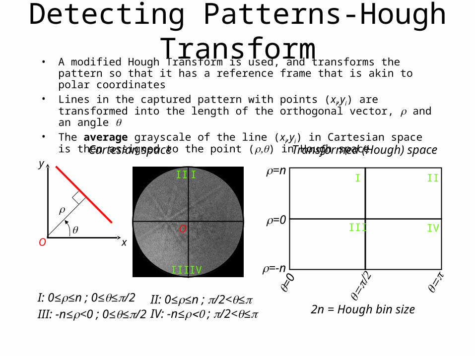
Detecting Patterns-Hough Transform• A modified Hough Transform is used, and transforms the pattern so that it has a

reference frame that is akin to polar coordinates • Lines in the captured pattern with points (xi,yi) are transformed into the length of the

orthogonal vector, r and an angle q• The average grayscale of the line (xi,yi) in Cartesian space is then assigned to the point

( ,r q) in Hough space

I: 0≤r≤n ; 0≤q≤p/2

III: -n≤r<0 ; 0≤q≤p/2

O

III

IIIIV

I II

IVIIIO x

y

r

qr=0

r=-n

r=n

q=0

=/

qp

2

=q pII: 0≤r≤n ; p/2<q≤p

IV: -n≤ <0r ; p/2<q≤p

Cartesian space Transformed (Hough) space

2n = Hough bin size

Detecting Patterns-The Hough of one band

• Since the patterns are composed of bands, and not lines, the observed peaks in Hough space are a collection of points and not just one discrete point

• Lines that intersect the band in Cartesian space are on average higher than those that do not intersect the band at all

Cartesian space Transformed (Hough) space

24

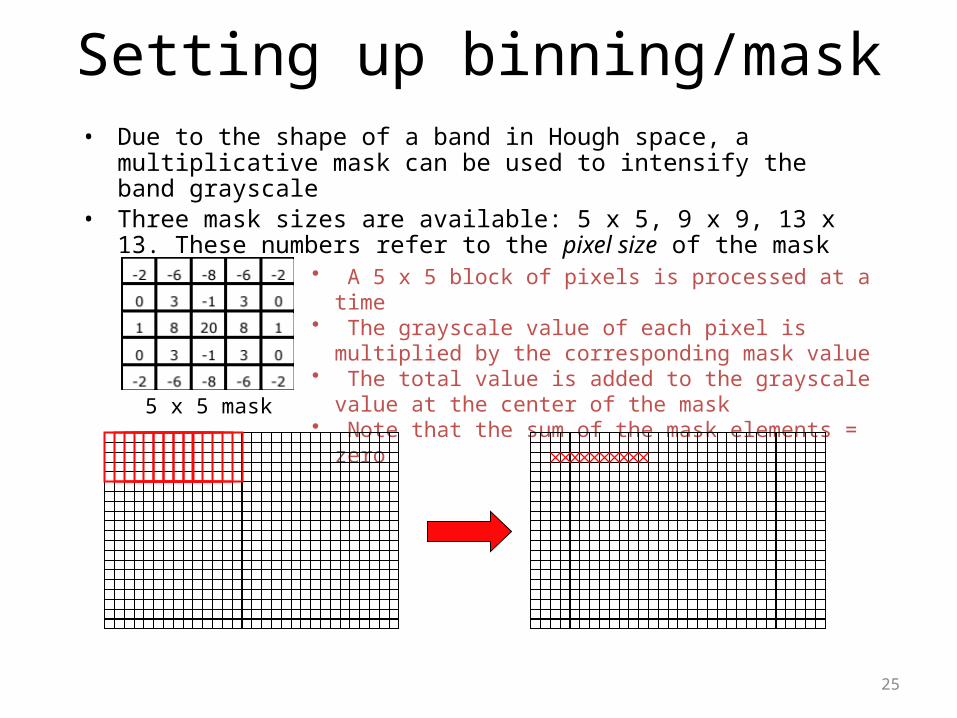
Setting up binning/mask• Due to the shape of a band in Hough space, a multiplicative mask can be used

to intensify the band grayscale• Three mask sizes are available: 5 x 5, 9 x 9, 13 x 13. These numbers refer to

the pixel size of the mask

5 x 5 mask

• A 5 x 5 block of pixels is processed at a time• The grayscale value of each pixel is multiplied by the

corresponding mask value• The total value is added to the grayscale value at the center of

the mask• Note that the sum of the mask elements = zero

25

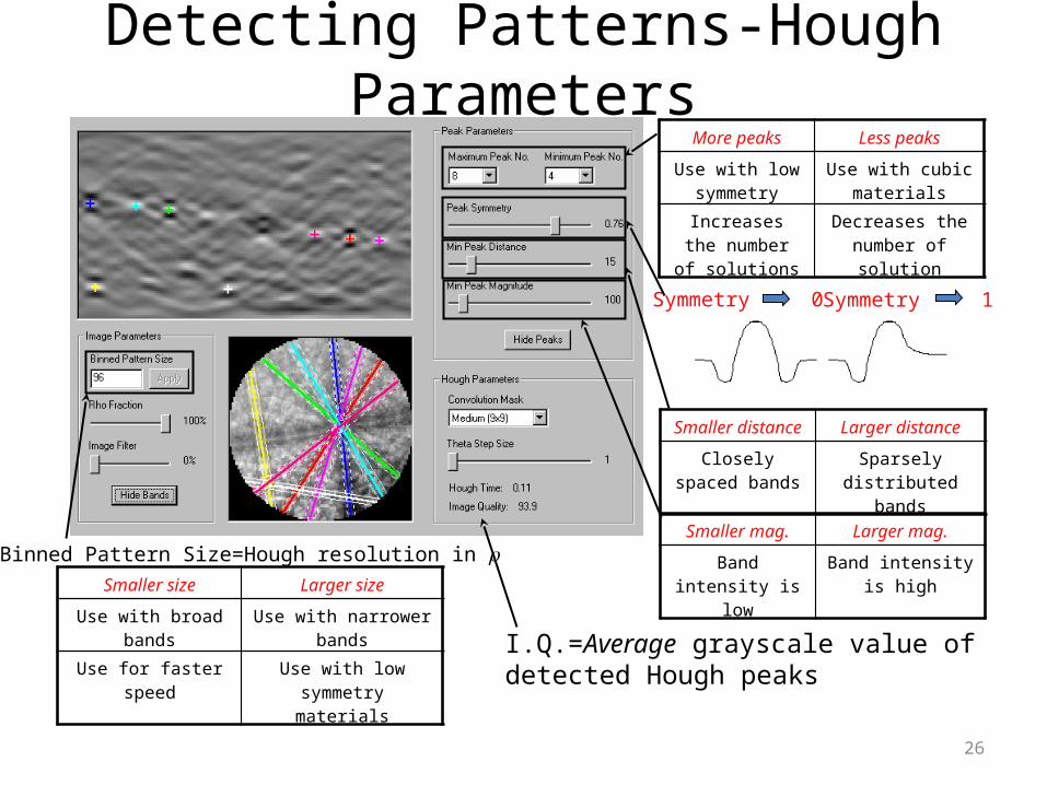
Detecting Patterns-Hough Parameters

Binned Pattern Size=Hough resolution in rSmaller size Larger size

Use with broad bands

Use with narrower bands

Use for faster speed Use with low symmetry materials

More peaks Less peaks

Use with low symmetry

Use with cubic materials

Increases the number of solutions

Decreases the number of solution

Smaller distance Larger distance

Closely spaced bands

Sparsely distributed bands

Symmetry 0 Symmetry 1

Smaller mag. Larger mag.

Band intensity is low

Band intensity is high

I.Q.=Average grayscale value of detected Hough peaks

26

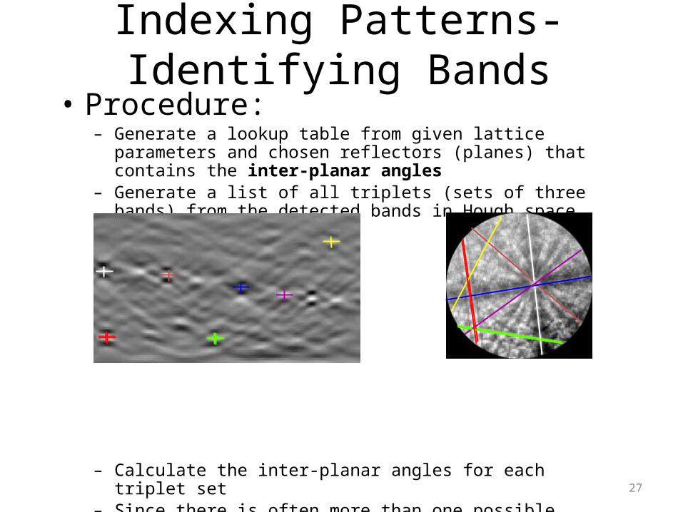
Indexing Patterns-Identifying Bands• Procedure:

– Generate a lookup table from given lattice parameters and chosen reflectors (planes) that contains the inter-planar angles

– Generate a list of all triplets (sets of three bands) from the detected bands in Hough space

– Calculate the inter-planar angles for each triplet set– Since there is often more than one possible solution for each triplet, a

method that uses all the bands needs to be implemented

27

Indexing Patterns-SettingsTolerance = How much angular deviation a plane is allowed while being a candidate

Lower Tolerance Larger Tolerance

Use if many bands are tightly bunched

Use with poorer patterns

Higher speed (eliminates possible

solutions)

Lower speed (more possible solutions)

Band widths: check if the theoretical width of bands should be considered during indexing

If multi-phase indexing is being used, a “best” solution for each phase will be calculated. These values assign a weight to each possible factor:- Votes: based on total votes for the solution/largest number of

votes for all phases- CI: ratio of CI/largest CI for all phases- Fit: fit for the solution/best (smallest) fit between all phases

The indexing solution of the phase with the largest Rank value is chosen as the solution for the pattern

28

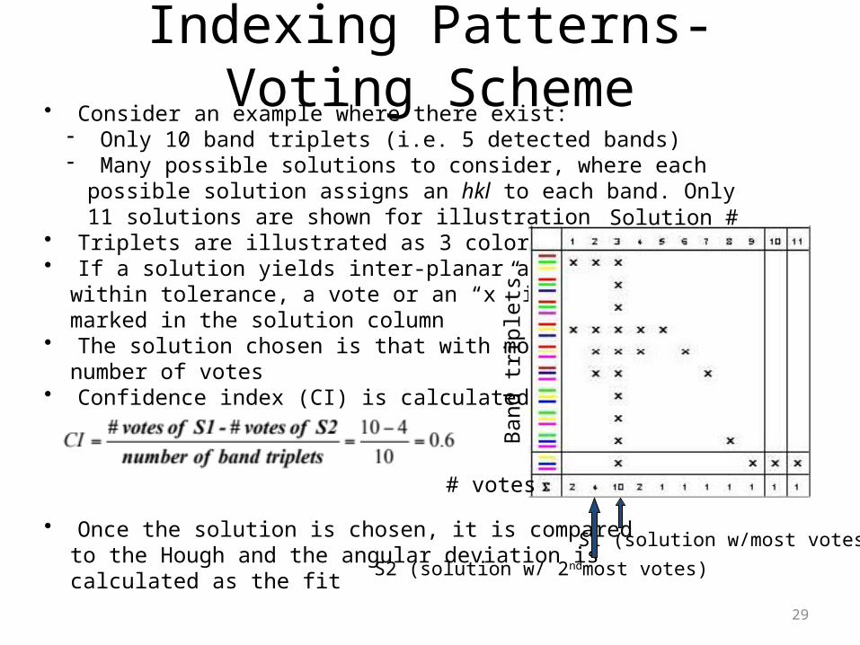
Indexing Patterns-Voting Scheme• Consider an example where there exist:

- Only 10 band triplets (i.e. 5 detected bands)- Many possible solutions to consider, where each possible solution assigns

an hkl to each band. Only 11 solutions are shown for illustration• Triplets are illustrated as 3 colored lines• If a solution yields inter-planar angles within tolerance, a vote or an “x” is marked in the solution column• The solution chosen is that with most number of votes• Confidence index (CI) is calculated as

• Once the solution is chosen, it is compared to the Hough and the angular deviation is calculated as the fit

Solution #

# votesBa

nd tr

iple

tsS1 (solution w/most votes)

S2 (solution w/ 2ndmost votes)

29

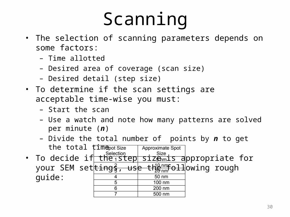
Scanning• The selection of scanning parameters depends on some factors:

– Time allotted– Desired area of coverage (scan size)– Desired detail (step size)

• To determine if the scan settings are acceptable time-wise you must:– Start the scan– Use a watch and note how many patterns are solved per minute (n)– Divide the total number of points by n to get the total time

• To decide if the step size is appropriate for your SEM settings, use the following rough guide:

30