underwater channel modeling for sonar applications...
TRANSCRIPT

1
UNDERWATER CHANNEL MODELING FOR SONAR APPLICATIONS
A THESIS SUBMITTED TOTHE GRADUATE SCHOOL OF NATURAL AND APPLIED SCIENCES
OFMIDDLE EAST TECHNICAL UNIVERSITY
BY
ERDAL EPCACAN
IN PARTIAL FULFILLMENT OF THE REQUIREMENTSFOR
THE DEGREE OF MASTER OF SCIENCEIN
ELECTRICAL AND ELECTRONICS ENGINEERING
FEBRUARY 2011
Approval of the thesis:
UNDERWATER CHANNEL MODELING FOR SONAR APPLICATIONS
submitted by ERDAL EPCACAN in partial fulfillment of the requirements for the degree ofMaster of Science in Electrical and Electronics Engineering Department, Middle EastTechnical University by,
Prof. Dr. Canan OzgenDean, Graduate School of Natural and Applied Sciences
Prof. Dr. Ismet ErkmenHead of Department, Electrical and Electronics Engineering
Assoc. Prof. Dr. Tolga CilogluSupervisor, Electrical and Electronics Engineering Dept., METU
Examining Committee Members:
Prof. Dr. Mustafa KuzuogluElectrical and Electronics Engineering Dept., METU
Assoc. Prof. Dr. Tolga CilogluElectrical and Electronics Engineering Dept., METU
Assoc. Prof Dr. Cagatay CandanElectrical and Electronics Engineering Dept., METU
Assoc. Prof Dr. Ali Ozgur YılmazElectrical and Electronics Engineering Dept., METU
Tevfik Bahadır Sarıkaya (M.Sc.)ASELSAN
Date:

I hereby declare that all information in this document has been obtained and presentedin accordance with academic rules and ethical conduct. I also declare that, as requiredby these rules and conduct, I have fully cited and referenced all material and results thatare not original to this work.
Name, Last Name: ERDAL EPCACAN
Signature :
iii
ABSTRACT
UNDERWATER CHANNEL MODELING FOR SONAR APPLICATIONS
Epcacan, Erdal
M.Sc., Department of Electrical and Electronics Engineering
Supervisor : Assoc. Prof. Dr. Tolga Ciloglu
February 2011, 70 pages
Underwater acoustic channel models have been studied in the context of communication and
sonar applications. Acoustic propagation channel in an underwater environment exhibits mul-
tipath, time-variability and Doppler effects. In this thesis, multipath fading channel models,
underwater physical properties and sound propagation characteristics are studied. An under-
water channel model for sonar applications is proposed. In the proposed model, the physical
characteristics of underwater environment are considered in a comprehensive manner. Exper-
iments/simulations were carried out using real-life data. Model parameters are estimated for a
specific location, scenario and physical conditions. The channel response is approximated by
fitting the model output to the recorded data. The optimization and estimation are conducted
in frequency domain using Mean Square Error criterion.
Keywords: Underwater Acoustic Channel, Fading Channel, Channel Simulation, Parameter
Optimization
iv
OZ
SONAR UYGULAMALARI ICIN SUALTI KANAL MODELLEMESI
Epcacan, Erdal
Yuksek Lisans, Elektrik ve Elektronik Muhendisligi Bolumu
Tez Yoneticisi : Doc. Dr. Tolga Ciloglu
Subat 2011, 70 sayfa
Sualtı akustik kanal modelleri iletisim ve sonar uygulamaları baglamında incelenmistir. Su-
altı ortamındaki akustik yayılma kanalı cok yollu yayılım, zaman degiskenligi ve Doppler
etkisi ozelliklerini sergilemektedir. Bu tezde, cok yollu sonumlenen kanal modelleri, su-
altı fiziksel ozellikleri ve ses yayılım ozellikleri incelenmistir. Sonar uygulamaları icin bir
sualtı kanal modeli onerilmistir. Onerilen modelde, sualtı ortamının fiziksel ozellikleri kap-
samlı bir sekilde goz onunde bulundurulmustur. Deneyler/simulasyonlar gercek hayat verileri
kullanılarak gerceklestirilmistir. Model parametreleri belirli bir konum, senaryo ve fiziksel
kosullar icin tahmin edilmistir. Model cıktısı kaydedilmis verilerle uyusturularak kanalın
durtu yanıtı yaklasık olarak bulunmustur. Optimizasyon ve tahmin islemleri Ortalama Kare-
sel Hata olcutu kullanılarak frekans bolgesinde yapılmaktadır.
Anahtar Kelimeler: Sualtı Akustik Kanal,Sonumlenen Kanallar, Kanal Simulasyonu, Degisken
Optimizasyonu
v

To My Family
vi
ACKNOWLEDGMENTS
I would like to express my deepest gratitude to my supervisor Assoc. Prof. Dr. Tolga Ciloglu
for his guidance, advice, criticism, encouragements and insight throughout the research.
Thanks to the examining committee members Prof. Dr. Mustafa Kuzuoglu, Assoc. Prof. Dr.
Cagatay Candan, Assoc. Prof. Dr. Ali Ozgur Yılmaz and Tevfik Bahadır Sarıkaya, Ms. Sc.,
for evaluating my work and for their valuable comments.
I would like to express my thanks especially to Mesude Civelekoglu, Oktay Sipahigil, Erdal
Mehmetcik, Berk Gurakan and all my friends for their suggestions, support and fellowship.
Deepest thanks to my family for their love, trust, understanding, and every kind of support
not only throughout my thesis but also throughout my life.
I would also like to thank Turkcell for their financial support during my graduate education.
vii
TABLE OF CONTENTS
ABSTRACT . . . . . . . . . . . . . . . . . . . . . . . . . . . . . . . . . . . . . . . . iv
OZ . . . . . . . . . . . . . . . . . . . . . . . . . . . . . . . . . . . . . . . . . . . . . v
ACKNOWLEDGMENTS . . . . . . . . . . . . . . . . . . . . . . . . . . . . . . . . . vii
TABLE OF CONTENTS . . . . . . . . . . . . . . . . . . . . . . . . . . . . . . . . . viii
LIST OF TABLES . . . . . . . . . . . . . . . . . . . . . . . . . . . . . . . . . . . . x
LIST OF FIGURES . . . . . . . . . . . . . . . . . . . . . . . . . . . . . . . . . . . . xi
CHAPTERS
1 INTRODUCTION . . . . . . . . . . . . . . . . . . . . . . . . . . . . . . . 1
1.1 Introduction . . . . . . . . . . . . . . . . . . . . . . . . . . . . . . 1
1.2 Outline . . . . . . . . . . . . . . . . . . . . . . . . . . . . . . . . . 3
2 STATISTICAL MULTIPATH FADING CHANNEL MODELS . . . . . . . . 5
2.1 Introduction . . . . . . . . . . . . . . . . . . . . . . . . . . . . . . 5
2.2 Time-Varying Channel [1] . . . . . . . . . . . . . . . . . . . . . . . 7
2.3 Narrowband Fading Model [1] . . . . . . . . . . . . . . . . . . . . 9
2.3.1 Autocorrelation, Cross Correlation and Power Spectral Den-sity . . . . . . . . . . . . . . . . . . . . . . . . . . . . . 13
2.3.2 Envelope and Power Distribution . . . . . . . . . . . . . . 17
2.4 Wideband Fading Model [1] . . . . . . . . . . . . . . . . . . . . . . 19
2.4.1 Power Delay Profile . . . . . . . . . . . . . . . . . . . . . 24
2.4.2 Coherence Bandwidth . . . . . . . . . . . . . . . . . . . 25
2.4.3 Doppler Power Spectrum and Channel Coherence Time . . 27
2.4.4 Transforms for Autocorrelation and Scattering Functions . 28
3 UNDERWATER ACOUSTIC CHANNEL . . . . . . . . . . . . . . . . . . . 30
3.1 The Ray Propagation Model [2] . . . . . . . . . . . . . . . . . . . . 31
viii
3.2 Speed Of Sound [2] . . . . . . . . . . . . . . . . . . . . . . . . . . 32
3.2.1 Underwater Sound Channels . . . . . . . . . . . . . . . . 33
3.3 Attenuation and Noise . . . . . . . . . . . . . . . . . . . . . . . . . 34
3.3.1 Spreading Loss . . . . . . . . . . . . . . . . . . . . . . . 34
3.3.2 Absorption Loss . . . . . . . . . . . . . . . . . . . . . . 34
3.3.3 Ambient Noise . . . . . . . . . . . . . . . . . . . . . . . 37
3.4 Multipath [2, 3, 4] . . . . . . . . . . . . . . . . . . . . . . . . . . . 40
3.4.1 Micro- and Macro-Multipath . . . . . . . . . . . . . . . . 40
3.5 The Doppler Effect [3, 2] . . . . . . . . . . . . . . . . . . . . . . . 44
3.6 Time Variability . . . . . . . . . . . . . . . . . . . . . . . . . . . . 47
4 SIMULATION OF UNDERWATER CHANNEL . . . . . . . . . . . . . . . 49
4.1 Introduction . . . . . . . . . . . . . . . . . . . . . . . . . . . . . . 49
4.2 Ambient Noise Generation . . . . . . . . . . . . . . . . . . . . . . 51
4.3 Time Delay and Received Power . . . . . . . . . . . . . . . . . . . 54
4.4 Doppler Spread and Doppler Power Spectrum . . . . . . . . . . . . 57
4.5 Loss . . . . . . . . . . . . . . . . . . . . . . . . . . . . . . . . . . 58
4.6 Multipath Formation and Micropath Effect . . . . . . . . . . . . . . 60
5 MODEL FITTING TO EXPERIMENTAL DATA . . . . . . . . . . . . . . . 65
5.1 Introduction . . . . . . . . . . . . . . . . . . . . . . . . . . . . . . 65
5.2 Optimization of Channel Parameters . . . . . . . . . . . . . . . . . 65
5.2.1 Optimizing the Sound Speed . . . . . . . . . . . . . . . . 65
5.2.2 Optimizing the Number of Paths . . . . . . . . . . . . . . 65
6 CONCLUSION . . . . . . . . . . . . . . . . . . . . . . . . . . . . . . . . . 66
6.1 Results . . . . . . . . . . . . . . . . . . . . . . . . . . . . . . . . . 66
6.2 Future Work . . . . . . . . . . . . . . . . . . . . . . . . . . . . . . 68
REFERENCES . . . . . . . . . . . . . . . . . . . . . . . . . . . . . . . . . . . . . . 69
ix
LIST OF TABLES
TABLES
Table 4.1 The physical conditions for Figure 4.7 . . . . . . . . . . . . . . . . . . . . 55
Table 6.1 The scenarios for the planned measurement . . . . . . . . . . . . . . . . . 68
x
LIST OF FIGURES
FIGURES
Figure 2.1 Multipath formation . . . . . . . . . . . . . . . . . . . . . . . . . . . . . 6
Figure 2.2 Delay spread, Tm, for a single pulse input . . . . . . . . . . . . . . . . . . 10
Figure 2.3 Delay spread, Tm, input and output in narrowband fading model for a single
symbol input . . . . . . . . . . . . . . . . . . . . . . . . . . . . . . . . . . . . . 11
Figure 2.4 Formation of output signal given in bottom panel of Figure 2.3 . . . . . . . 11
Figure 2.5 Bessel Function versus fDτ . . . . . . . . . . . . . . . . . . . . . . . . . 16
Figure 2.6 PSD of rI and rQ . . . . . . . . . . . . . . . . . . . . . . . . . . . . . . . 17
Figure 2.7 Input signal consisting of two cascaded symbols . . . . . . . . . . . . . . 20
Figure 2.8 The output signal for narrowband fading model corresponding to input
given in Figure 2.7 . . . . . . . . . . . . . . . . . . . . . . . . . . . . . . . . . . 20
Figure 2.9 The output signal for wideband fading model corresponding to input given
in Figure 2.7 . . . . . . . . . . . . . . . . . . . . . . . . . . . . . . . . . . . . . 21
Figure 2.10 Delay spread, Tm, input and corresponding output for wideband fading model 22
Figure 2.11 Power Delay Profile, RMS Delay and Coherence Bandwidth . . . . . . . . 27
Figure 2.12 Doppler Power Spectrum, Doppler Spread and Coherence Time . . . . . . 28
Figure 2.13 Fourier transform relations for AC(∆ f ; ∆t), Ac(τ; ∆t), S C(∆ f ; ρ) and S c(τ; ρ) 29
Figure 3.1 Reflection and refraction in shallow and deep water respectively . . . . . . 32
Figure 3.2 Speed profile in deep and shallow water . . . . . . . . . . . . . . . . . . . 33
Figure 3.3 Attenuation of sound wave in sea water due to absorption . . . . . . . . . 35
Figure 3.4 Average signal power with respect to range . . . . . . . . . . . . . . . . . 37
Figure 3.5 Noise Power Spectral Density for ship activity=0 and wind speed=0, 5, 10
m/s. . . . . . . . . . . . . . . . . . . . . . . . . . . . . . . . . . . . . . . . . . . 39
xi
Figure 3.6 SNR depends on frequency and distance by the factor 1/A(r,f)N(f) . . . . . 39
Figure 3.7 Input delay spread function for a channel with five paths . . . . . . . . . . 43
Figure 3.8 Doppler effect for the case where the path between the transmitter and re-
ceiver increases due to relative motion during the propagation of the signal. Upper
part belongs to transmitted signal whereas the lower part belongs to received signal
for a single path only. ’a’ is Doppler ratio . . . . . . . . . . . . . . . . . . . . . . 45
Figure 4.1 PSD relation between input and output of a filter . . . . . . . . . . . . . . 51
Figure 4.2 Underwater ambient noise generation by using white Gaussian noise . . . 51
Figure 4.3 Theoretical and simulated underwater ambient noise Power Spectral Den-
sities for wind speed=0 m/s . . . . . . . . . . . . . . . . . . . . . . . . . . . . . 52
Figure 4.4 Time domain ambient noise signal . . . . . . . . . . . . . . . . . . . . . . 52
Figure 4.5 Spectrogram of ambient noise for wind speeds 0 and 10 m/s . . . . . . . . 53
Figure 4.6 Spectrogram of ambient noise for wind speeds 15 and 20 m/s . . . . . . . 53
Figure 4.7 Received signals from different paths with different delay times; losses are
ignored. . . . . . . . . . . . . . . . . . . . . . . . . . . . . . . . . . . . . . . . 54
Figure 4.8 Received power and the received signal for 500 m horizontal distance . . . 55
Figure 4.9 Received power and the received signal for 200 m horizontal distance . . . 56
Figure 4.10 Relative times for 200m and 500m distances . . . . . . . . . . . . . . . . 56
Figure 4.11 Doppler shifts in the received signal, where the input frequency is 10KHz . 57
Figure 4.12 Doppler power spectrum for a relative motion of +5m/s . . . . . . . . . . 58
Figure 4.13 Paths with spreading and absorption loss mechanisms only . . . . . . . . . 60
Figure 4.14 Paths with all loss mechanisms . . . . . . . . . . . . . . . . . . . . . . . 61
Figure 4.15 Random method multipath formation . . . . . . . . . . . . . . . . . . . . 62
Figure 4.16 Image method multipath formation . . . . . . . . . . . . . . . . . . . . . 62
Figure 4.17 Micropath effect is seen on the paths. Note that there is no micropath effect
on the first path . . . . . . . . . . . . . . . . . . . . . . . . . . . . . . . . . . . 63
Figure 4.18 Micropath effect simulator . . . . . . . . . . . . . . . . . . . . . . . . . . 64
xii
CHAPTER 1
INTRODUCTION
1.1 Introduction
Increasing interest in defense applications, off-shore oil industry, and other commercial op-
erations in underwater environment provides underwater research to become more popular.
Therefore in correlation to increase in interest, the number of research studies and appli-
cations that are conducted to explore underwater environment is increasing. In underwater
environment, electromagnetic waves are subject to high attenuation and can only travel very
short distances and therefore the only way that navigation, communication and other wireless
applications can be done is through acoustic methods [5].
Underwater acoustic channel is difficult to work and has inherent problems. Difficulty comes
from channel characteristics such as attenuation, multipath fading, time varying characteris-
tics and inhomogeneities of the channel [6]. The attenuation in underwater channel is pro-
portional to distance between the source and receiver and to square of the frequency of the
signal, making the channel severely band limited[7]. Therefore underwater systems work at
small frequencies, such as, on the order of tens of kHz. In addition to that, attenuation occurs
due to reflections from bottom and surface of the channel.
In underwater channel multipaths occur due to reflections and refractions. Reflections gen-
erally occur from the bottom and the surface of the underwater channel whereas refractions
occur due to sound channels created by the inhomogeneities of the sound speed. The number
of multipaths reaching the receiver side can be very large, however the ones under noise level
are ignored.
Internal and surface waves in an underwater channel continuously change the channel char-
1
acteristics by changing the reflection points of the transmitted signal. Moreover, the motion
of these waves creates a Doppler effect in the channel. Underwater channel shows inhomo-
geneities in speed, temperature and salinity. The speed, temperature and salinity change as
the depth of water changes. These variables may also change in time and may be different for
the same depth of different places. Therefore, it can be said that the channel impulse response
changes both spatially and temporarily. In addition to that as the place of the transmitter
and receiver changes the channel impulse response also changes since the channel impulse
response depends on the positions of the transmitter and receiver also.
Underwater channel is a double spread channel. It exhibits both dispersion in time (delay
spread) and in frequency (Doppler spread) [7].
There are many of underwater channel models. Most of the channels implemented have used
Ray theory as basis [8]. Galvin and Coates [9] have simulated the stochastic property of the
channel (fading statistics) however they have not used physical properties of the underwater
channel. The channel is implemented as tapped delayed sum of input, where the tap gains are
complex random processes. This method was also used in [10].
The channel also has been described and simulated as a tapped delay line with variable delays,
and stochastic tap gains in [11]. In addition to that, physical loss and Doppler factors are
included using Bellhop acoustic toolbox [12].
In [13] the channel simulation contains physical properties of the channel, however the Doppler
effect and micro-path effect is not included in simulation. The paths are formed by image
method and with no randomness, therefore for the same number of paths under the same
physical conditions the channel impulse response is found to be the same. In addition to
that the surface, bottom and absorption loss are pre-determined which should be calculated
according to depth, grazing angles and signal frequency.
In [14] the model is simulated using propagation loss and multipath fading properties. The
Doppler effect and reflection loss parameters are not simulated.
In [15] multipath and micropath effects are implemented with loss delay and Doppler effect.
The model in [15] is created using [16] and is physical based however there is no acoustical
propagation physics mentioned such as spreading and absorption. In addition to that ambient
noise has not been modeled. The formation of paths is random but multiple reflections are not
2
mentioned.
In [17] the physical properties of the underwater channel and multipath fading statistics are
included. The model includes surface and bottom loss effects but they are taken to be constant
for all cases where they should depend on the grazing angle and bottom type. Moreover the
Doppler shift is not calculated but has been taken as a constant function of relative speed only
where the sound speed should also be calculated and used to find Doppler shift.
In the model used for this thesis, nearly all physical properties of the underwater channel
with multipath fading statistics have been used. The motion of the transmitter and emitter
including the frequency spread due to motion of waves have been implemented. All types of
the losses including grazing angles are also modeled. Moreover the ambient noise has also
been modeled. Inhomogeneities of speed, temperature and salinity are included in the model.
The simulation is done in time domain using discrete data sampled at a sampling frequency
of experiments conducted. However, analyses are done in both time and frequency domains.
Furthermore the simulation outputs are observed and illustrated in both time and frequency
domains.
1.2 Outline
The outline of this thesis is as follows: Chapter 2 gives a review about general multipath
fading channel. Time varying characteristics of the channel are described by using a gen-
eral channel impulse response for a multipath fading channel. Types of fading models and
necessary conditions to obtain these types are presented. Characterization of channel accord-
ing to these types using the channel impulse response and related functions are investigated.
Definitions about a multipath fading channel and characterization functions and the relation
between these functions are given.
In Chapter 3, physical properties of an underwater environment are given. Mathematical
models of propagation loss, ambient noise, sound speed variation and ray propagation are
presented. Channel impulse response, multipath models and Doppler effects specific to an
underwater environment are explained.
The method and results of the simulations of the underwater channel model are presented
3
in Chapter 4. Time and frequency representations of the output of the channel for specific
scenarios and input are investigated. The characterization functions Power Delay Profile and
Doppler Power Spectrum obtained from these specific scenarios’ outputs are discussed. The
channel characteristic parameters, Delay Spread and Doppler Spread have been determined
from these characterization functions.
In Chapter 5, the channel parameters are optimized and simulated channel impulse response
is approximated to a real channel impulse response under specific scenarios. Undetermined
parameters were Sound Speed and the Number of Multipaths. In Section 5.2.1 the sound speed
is optimized by using a minimum mean square error criterion in frequency domain. Finally,
in Section 5.2.2 the optimum number of paths for which the channel is best approximated is
found for two specific scenarios. The approximation is illustrated by giving Doppler Power
Spectra of the simulated and the real channel before and after optimization.
Conclusions and future work are given in Chapter 6.
4
CHAPTER 2
STATISTICAL MULTIPATH FADING CHANNEL MODELS
2.1 Introduction
Underwater channels are multipath fading channels therefore investigation of underwater
channel will be started with studying multipath fading channels. In this chapter a general
multipath fading channel will be considered. Multipath channel and fading phenomenon will
be defined and necessary conditions and assumptions for different types of fading will be
given. Some important parameters that are related to multipath fading communication chan-
nels and that will be mentioned in this thesis are as follows:
Multipath Propagation: In a wireless communication system, due to reflections caused
by environmental conditions, natural and man-made objects through the channel and due to
channel characteristics, multiple of transmitted signals are obtained at receiver side. Figure
2.1 shows a multipath formation for a wireless channel.
Fading: In multipath propagation, all paths having different amplitude, delay, phase shift
and frequency shift are added on the receiver side, in this addition the signal amplitude can
severely decrease or increase. This phenomenon is called multipath fading [18]
Delay: The transmitted signal reaches the receiver after some time during propagation due
to fact that propagation speed of the transmitted signal is not infinite.
5
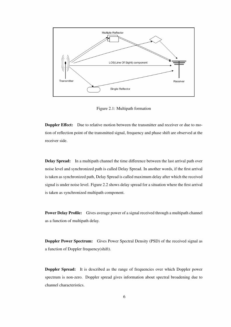
Figure 2.1: Multipath formation
Doppler Effect: Due to relative motion between the transmitter and receiver or due to mo-
tion of reflection point of the transmitted signal, frequency and phase shift are observed at the
receiver side.
Delay Spread: In a multipath channel the time difference between the last arrival path over
noise level and synchronized path is called Delay Spread. In another words, if the first arrival
is taken as synchronized path, Delay Spread is called maximum delay after which the received
signal is under noise level. Figure 2.2 shows delay spread for a situation where the first arrival
is taken as synchronized multipath component.
Power Delay Profile: Gives average power of a signal received through a multipath channel
as a function of multipath delay.
Doppler Power Spectrum: Gives Power Spectral Density (PSD) of the received signal as
a function of Doppler frequency(shift).
Doppler Spread: It is described as the range of frequencies over which Doppler power
spectrum is non-zero. Doppler spread gives information about spectral broadening due to
channel characteristics.
6
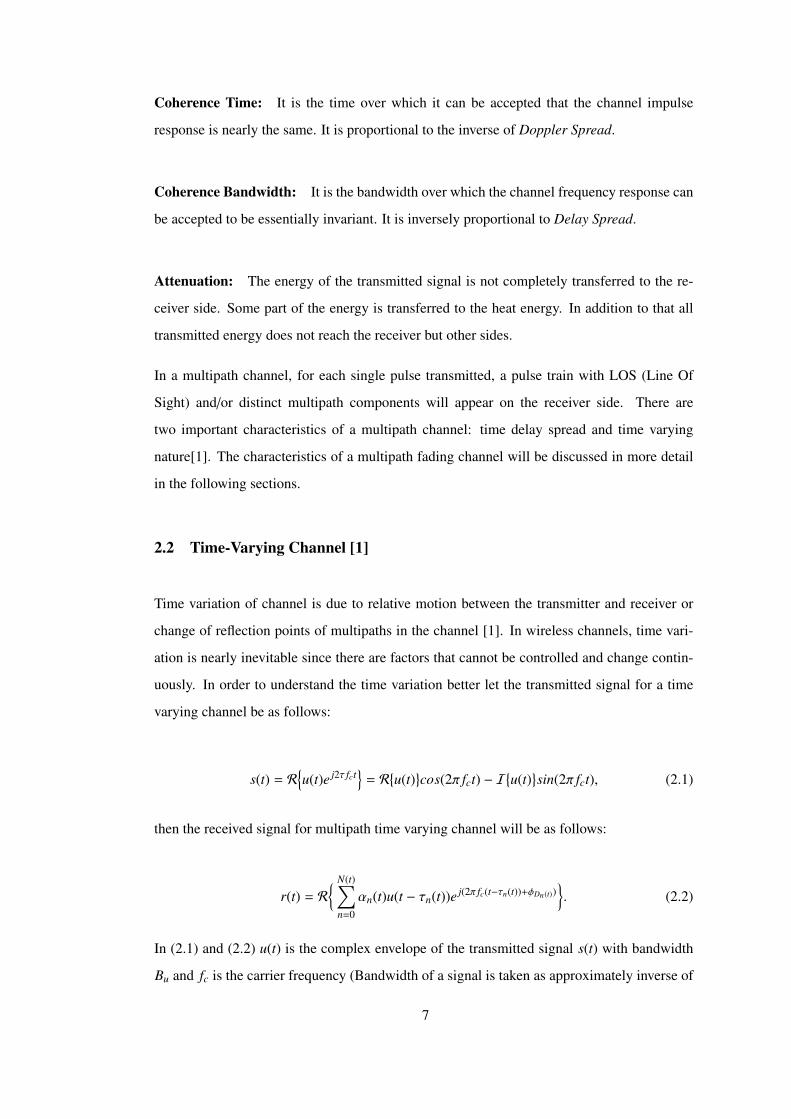
Coherence Time: It is the time over which it can be accepted that the channel impulse
response is nearly the same. It is proportional to the inverse of Doppler Spread.
Coherence Bandwidth: It is the bandwidth over which the channel frequency response can
be accepted to be essentially invariant. It is inversely proportional to Delay Spread.
Attenuation: The energy of the transmitted signal is not completely transferred to the re-
ceiver side. Some part of the energy is transferred to the heat energy. In addition to that all
transmitted energy does not reach the receiver but other sides.
In a multipath channel, for each single pulse transmitted, a pulse train with LOS (Line Of
Sight) and/or distinct multipath components will appear on the receiver side. There are
two important characteristics of a multipath channel: time delay spread and time varying
nature[1]. The characteristics of a multipath fading channel will be discussed in more detail
in the following sections.
2.2 Time-Varying Channel [1]
Time variation of channel is due to relative motion between the transmitter and receiver or
change of reflection points of multipaths in the channel [1]. In wireless channels, time vari-
ation is nearly inevitable since there are factors that cannot be controlled and change contin-
uously. In order to understand the time variation better let the transmitted signal for a time
varying channel be as follows:
s(t) = R{u(t)e j2τ fct
}= R
{u(t)
}cos(2π fct) − I
{u(t)
}sin(2π fct), (2.1)
then the received signal for multipath time varying channel will be as follows:
r(t) = R
{ N(t)∑n=0
αn(t)u(t − τn(t))e j(2π fc(t−τn(t))+φDn(t))}. (2.2)
In (2.1) and (2.2) u(t) is the complex envelope of the transmitted signal s(t) with bandwidth
Bu and fc is the carrier frequency (Bandwidth of a signal is taken as approximately inverse of
7
its symbol duration i.e. B ≈ 1/Ts where Ts is symbol duration). In (2.2), the received signal
r(t) is the combination of LOS component (n = 0) and other delayed multipath components.
In (2.2), N(t), αn(t), τn(t) and φDn(t) are the number of resolvable multipath components,
amplitude of the nth component, corresponding delay and Doppler phase shift, respectively.
Two multipath components with delays τn and τm are resolvable if |τn − τm| � 1/(Bu) other-
wise they are unresolvable since u(t − τn) ≈ u(t − τm). Each nth path given in (2.2) may be
reflected from a single reflector or multiple reflectors clustered together as shown in Figure
2.1.
In case of multiple reflectors the delay of the multipaths will be very close and are combined
to be a single multipath component with rapidly varying amplitude due to constructive and
destructive addition of multipath components causing non resolvable paths. Generally wide-
band channels have resolvable multipath components, however, narrowband channels have
non resolvable multipath components.
In (2.2) the received signal can be simplified by letting
φn(t) = 2π fcτn(t) − φDn(t), (2.3)
then r(t) becomes as follows:
r(t) = R
{[ N(t)∑n=0
αn(t)e− jφn(t)u(t − τn(t))]e j2π fct
}. (2.4)
The amplitude αn(t) depends on loss and shadowing and φn(t) depends on delay and Doppler.
Therefore αn(t) and φn(t) can be accepted as independent random processes. They are char-
acterized as random process since they change over time.
The received signal can be represented as the convolution of the baseband input signal u(t) and
time-varying impulse response c(τ, t) and followed by up conversion with carrier frequency
fc:
r(t) = R
{( ∫ ∞
−∞
c(τ, t)u(t − τ)dτ)e j2π fct
}(2.5)
8
Here c(τ, t) is the channel impulse response and has two variables: t is the time that the
corresponding impulse is received and t − τ is the time that the impulse is sent.
When (2.4) and (2.5) are compared, c(τ, t) is obtained as follows:
c(τ, t) =
N(t)∑n=0
αn(t)e− jφn(t)δ(τ − τn(t)). (2.6)
In some cases, in the channel there can be continuum of multipath delays then the sum in (2.6)
becomes an integral so c(τ, t) becomes as follows (time-varying complex amplitude associated
with each delay τ):
c(τ, t) =
∫α(ξ, t)e− jφ(ξ,t)δ(τ − ξ) = α(τ, t)e− jφ(τ,t). (2.7)
In the following sections this impulse response, c(τ, t), will be used to characterize the channel
model.
Fading model can be defined according to relationship between delay spread, Tm and signal
bandwidth, B. If the spread of time delays associated to LOS and all other components is
smaller than the inverse of signal bandwidth (Tm << B−1) then components are non resolv-
able(narrowband fading model), otherwise the components are resolvable (wideband fading
model) these cases will be discussed in more detail in Section 2.3 and 2.4 respectively. Delay
spread can be measured in different ways but the important point is the choice of component
to which receiver is synchronized, say here it is τx, then the delay spread is calculated as
Tm = maxn|τn−τx|. For a single pulse input, the delay spread Tm is shown in Figure 2.2. Here
it should be noted that there are infinite number of multipath components but the one whose
power has gone under noise level should not contribute to the delay spread. It is obvious that
the multipath delays vary in the time so Tm becomes a random variable.
2.3 Narrowband Fading Model [1]
As discussed in Section 2.2 when Tm � B−1, that is when delay spread is smaller than
bandwidth of the signal, narrowband fading model is obtained. In this case u(t − τi) ≈ u(t)
since τi ≤ Tm ∀i, then (2.4) becomes as follows:
9
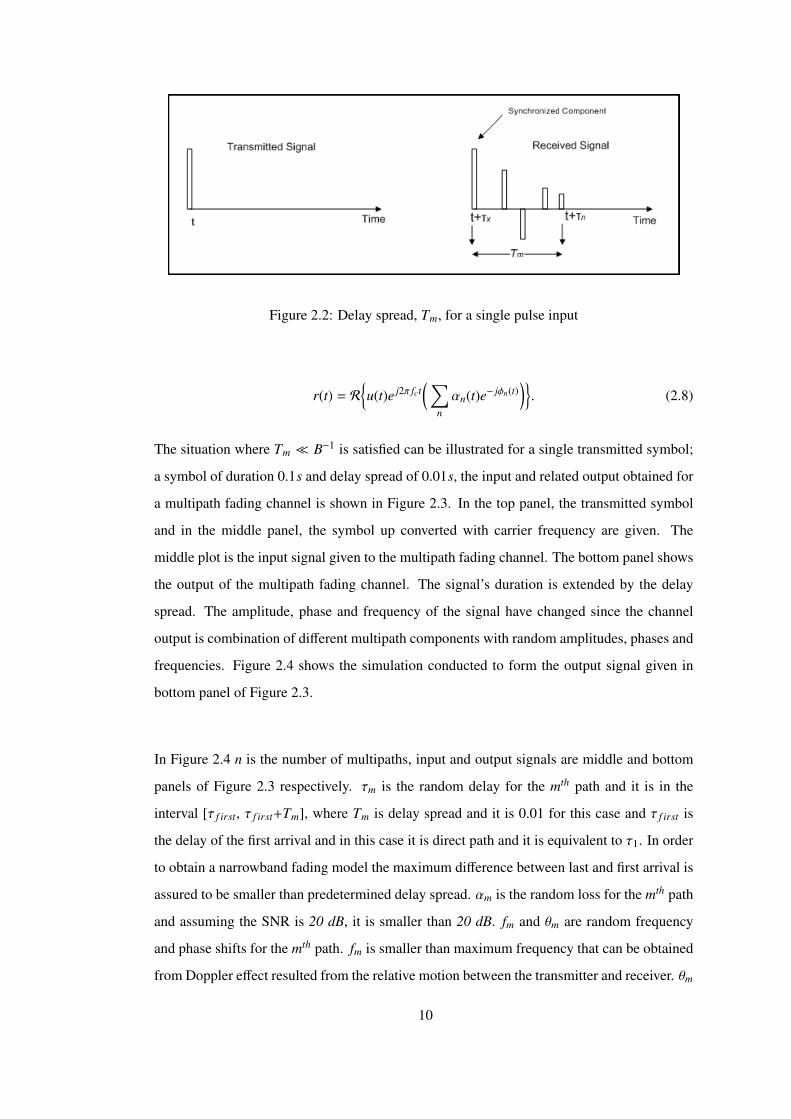
Figure 2.2: Delay spread, Tm, for a single pulse input
r(t) = R
{u(t)e j2π fct
(∑n
αn(t)e− jφn(t))}. (2.8)
The situation where Tm � B−1 is satisfied can be illustrated for a single transmitted symbol;
a symbol of duration 0.1s and delay spread of 0.01s, the input and related output obtained for
a multipath fading channel is shown in Figure 2.3. In the top panel, the transmitted symbol
and in the middle panel, the symbol up converted with carrier frequency are given. The
middle plot is the input signal given to the multipath fading channel. The bottom panel shows
the output of the multipath fading channel. The signal’s duration is extended by the delay
spread. The amplitude, phase and frequency of the signal have changed since the channel
output is combination of different multipath components with random amplitudes, phases and
frequencies. Figure 2.4 shows the simulation conducted to form the output signal given in
bottom panel of Figure 2.3.
In Figure 2.4 n is the number of multipaths, input and output signals are middle and bottom
panels of Figure 2.3 respectively. τm is the random delay for the mth path and it is in the
interval [τ f irst, τ f irst+Tm], where Tm is delay spread and it is 0.01 for this case and τ f irst is
the delay of the first arrival and in this case it is direct path and it is equivalent to τ1. In order
to obtain a narrowband fading model the maximum difference between last and first arrival is
assured to be smaller than predetermined delay spread. αm is the random loss for the mth path
and assuming the SNR is 20 dB, it is smaller than 20 dB. fm and θm are random frequency
and phase shifts for the mth path. fm is smaller than maximum frequency that can be obtained
from Doppler effect resulted from the relative motion between the transmitter and receiver. θm
10
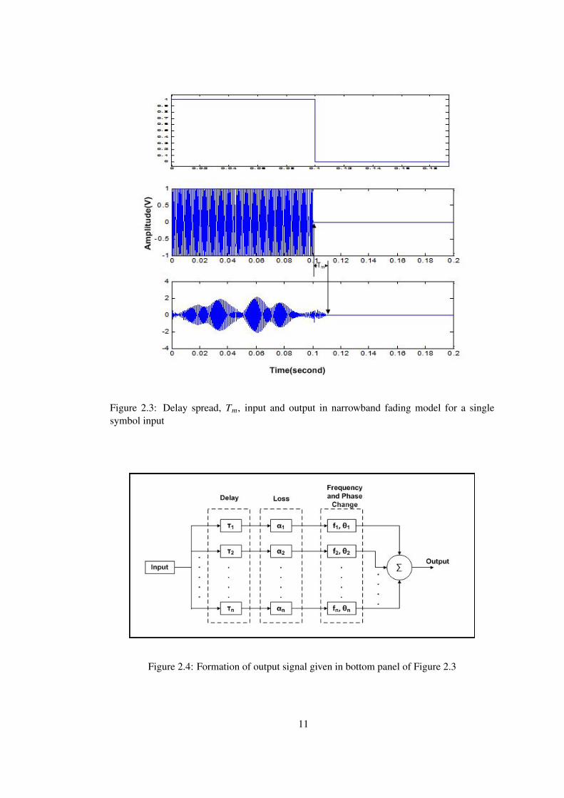
Figure 2.3: Delay spread, Tm, input and output in narrowband fading model for a singlesymbol input
Figure 2.4: Formation of output signal given in bottom panel of Figure 2.3
11
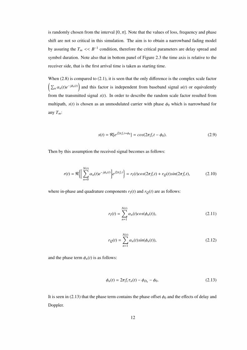
is randomly chosen from the interval [0, π]. Note that the values of loss, frequency and phase
shift are not so critical in this simulation. The aim is to obtain a narrowband fading model
by assuring the Tm << B−1 condition, therefore the critical parameters are delay spread and
symbol duration. Note also that in bottom panel of Figure 2.3 the time axis is relative to the
receiver side, that is the first arrival time is taken as starting time.
When (2.8) is compared to (2.1), it is seen that the only difference is the complex scale factor(∑n αn(t)e− jφn(t)
)and this factor is independent from baseband signal u(t) or equivalently
from the transmitted signal s(t). In order to describe the random scale factor resulted from
multipath, s(t) is chosen as an unmodulated carrier with phase φ0 which is narrowband for
any Tm:
s(t) = R{e j2π fct+φ0
}= cos(2π fct − φ0). (2.9)
Then by this assumption the received signal becomes as follows:
r(t) = R
{[ N(t)∑n=0
αn(t)e− jφn(t)]e j2π fct
}= rI(t)cos(2π fct) + rQ(t)sin(2π fct), (2.10)
where in-phase and quadrature components rI(t) and rQ(t) are as follows:
rI(t) =
N(t)∑n=1
αn(t)cos(φn(t)), (2.11)
rQ(t) =
N(t)∑n=1
αn(t)sin(φn(t)), (2.12)
and the phase term φn(t) is as follows:
φn(t) = 2π fcτn(t) − φDn − φ0. (2.13)
It is seen in (2.13) that the phase term contains the phase offset φ0 and the effects of delay and
Doppler.
12
In case of large N(t), by using Central Limit Theorem and the fact that αn(t) and φn(t) are
stationary and ergodic, it can be shown that rI(t) and rQ(t) can be approximated to be jointly
Gaussian. In case of small N(t), the Gaussian property still holds if αn(t) are Rayleigh dis-
tributed and φn(t) are uniformly distributed on [−π, π] [1].
2.3.1 Autocorrelation, Cross Correlation and Power Spectral Density
In this section autocorrelation and cross-correlation functions of the in-phase and quadra-
ture components, rI(t) and rQ(t), of the received signal are derived. In the derivation, some
basic assumptions are made, these assumptions are applicable in the case of absence of a
dominant LOS component. In this section it is assumed that the variables; amplitude αn(t),
multipath delay τn(t) and Doppler frequency fDN (t) change slowly enough over the inter-
ested time interval that they are assumed to be constant, that is αn(t) ≈ α, τn(t) ≈ τ and
fDN (t) ≈ fDN . Under this assumption the Doppler phase shift and phase of the nth term
become as φDn(t) =∫
t 2π fDndt = 2π fDn t and φn(t) = 2π fcτn − 2π fDn t − φ0 respectively.
The next assumption which is a key and a reasonable assumption is that the term 2π fcτn for
the nth term changes more rapidly than other terms in the phase. This is because of the fact
that fc is large and for a small change in τn, 2π fcτn can go through a 360 degree rotation.
Therefore the phase term is assumed to be uniformly distributed over [−π, π]. With these
assumptions we get the expected value of the in-phase part of the received signal as follows:
E[rI(t)
]= E
[∑n
αncosφn(t)]
=∑
n
E[αn]E[cosφn(t)] = 0. (2.14)
Note that in (2.14) the second equality comes from independence of αn and φn and last
equality comes from uniform distribution of φn around zero. Similarly it can be shown that
E[rQ(t)] = 0. Hence the received signal has also zero-mean, E[r(t)] = 0, and since rI(t) and
rQ(t) are jointly Gaussian the received signal is zero-mean Gaussian. Note that these mean
values are valid in the case when there is no dominant LOS component in the received sig-
nal. If there is a LOS component, the received signal’s phase is affected by the phase of LOS
component and random uniform phase assumption is no longer valid.
The autocorrelation of in-phase and quadrature components using independency of αn and φn
and independence of φn and φm, n , m, can be obtained as follows:
13
E[rI(t)rQ(t)] =
[∑n
αncosφn(t)∑
m
αmsinφm(t)]
= 0. (2.15)
This shows that rI(t) and rQ(t) are uncorrelated and since they are jointly Gaussian process,
they are independent. In a similar way as in (2.15) the autocorrelation of rI(t) is obtained as
follows:
ArI (t, τ) = E[rI(t)rI(t + τ)] =∑
n
E[α2n]E[cosφn(t)cosφn(t + τ)]. (2.16)
Making the substition φn(t) = 2π fcτn − 2π fDn t − φ0 and considering the fact that 4π fcτn term
changes more rapidly than other terms and since it is uniformly distributed (2.16) reduces to
ArI (t, τ) = 1/2∑
n
E[α2n]E[cos(2π fDnτ)] = 1/2
∑n
E[α2n]cos(2πvτcosθn/λ), (2.17)
since fDn = vcosθn/λ where λ = c/ fc. Note that ArI (t, τ) depends only on τ, that is ArI (t, τ) =
ArI (τ) therefor rI(t) is wide-sense stationary (WSS) random process. Similarly it can be shown
that quadrature component rQ(t) is also WSS with autocorrelation function ArI (τ) = ArQ(τ).
Moreover the cross-correlation between in-phase and quadrature components also depends
only on τ and it is given as follows:
ArI ,rQ(t, τ) = ArI ,rQ(τ) = E[rI(t)rQ(t + τ)]
= −0.5∑
n
E[α2n]sin(2πvτcosθn/λ)
= −E[rQ(t)rI(t + τ)]. (2.18)
Using (2.17) and (2.18) it can be shown that the received signal r(t) is also WSS with auto-
correlation function
Ar(τ) = E[r(t)r(t + τ)] = ArI (τ)cos(2π fcτ) + ArIrQ(τ)sin(2π fcτ) (2.19)
14
To simplify equations (2.18) and (2.17) a model called uniform scattering environment is
used [1]. In this model, it is assumed that each multipath component has an angle of arrival
θn = n∆θ where ∆θ = 2π/N. Moreover it is assumed that each multipath component has the
same received power that is E[α2n] = 2Pr/N where Pr is the total received power.
Considering these assumptions and making the substition N = 2π/∆θ (2.17) becomes
ArI =Pr
2π
N∑n=1
cos(2πvτcosn∆θ/λ)∆θ (2.20)
Assuming infinite number of multipaths(N → ∞,∆θ → 0) with uniform scattering the sum-
mation in (2.20) becomes an integral:
ArI =Pr
2π
∫cos(2πvτcosθ/λ)dθ = Pr J0(2π fDτ), (2.21)
where
J0(x) =1π
∫ π
0e− jxcosθdθ (2.22)
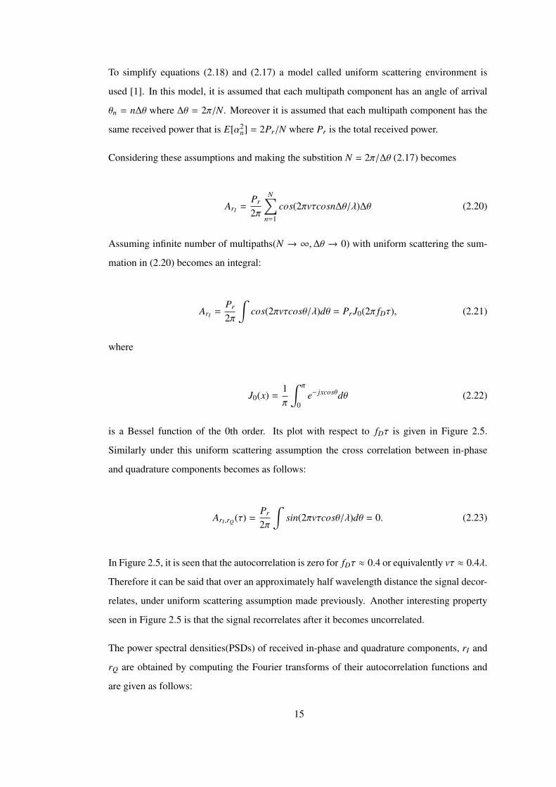
is a Bessel function of the 0th order. Its plot with respect to fDτ is given in Figure 2.5.
Similarly under this uniform scattering assumption the cross correlation between in-phase
and quadrature components becomes as follows:
ArI ,rQ(τ) =Pr
2π
∫sin(2πvτcosθ/λ)dθ = 0. (2.23)
In Figure 2.5, it is seen that the autocorrelation is zero for fDτ ≈ 0.4 or equivalently vτ ≈ 0.4λ.
Therefore it can be said that over an approximately half wavelength distance the signal decor-
relates, under uniform scattering assumption made previously. Another interesting property
seen in Figure 2.5 is that the signal recorrelates after it becomes uncorrelated.
The power spectral densities(PSDs) of received in-phase and quadrature components, rI and
rQ are obtained by computing the Fourier transforms of their autocorrelation functions and
are given as follows:
15
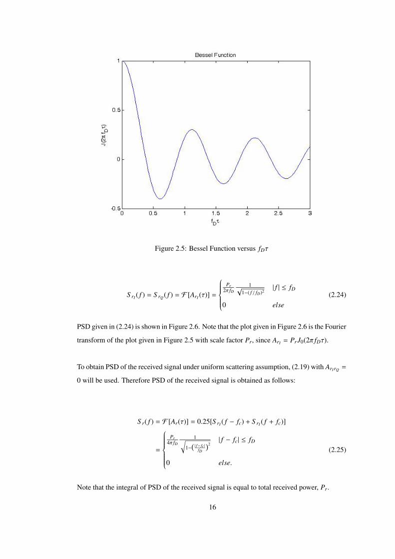
Figure 2.5: Bessel Function versus fDτ
S rI ( f ) = S rQ( f ) = F [ArI (τ)] =
Pr
2π fD1√
1−( f / fD)2| f | ≤ fD
0 else(2.24)
PSD given in (2.24) is shown in Figure 2.6. Note that the plot given in Figure 2.6 is the Fourier
transform of the plot given in Figure 2.5 with scale factor Pr, since ArI = Pr J0(2π fDτ).
To obtain PSD of the received signal under uniform scattering assumption, (2.19) with ArIrQ =
0 will be used. Therefore PSD of the received signal is obtained as follows:
S r( f ) = F [Ar(τ)] = 0.25[S rI ( f − fc) + S rI ( f + fc)]
=
Pr
4π fD1√
1−(| f− fc |
fD
)2| f − fc| ≤ fD
0 else.
(2.25)
Note that the integral of PSD of the received signal is equal to total received power, Pr.
16
Figure 2.6: PSD of rI and rQ
The PSD given in (2.25) models the power spectral density related to multipaths as a function
of Doppler frequency. Therefore it can be seen as distribution of random frequency due to
Doppler. It is seen that the PSD of in-phase and quadrature components goes to infinity at
f = ± fD and PSD of the received signal goes to infinity at f = ± fc ± fD, in practice this is
not true since uniform scattering is just an approximation. However, they take their maximum
values at these points. PSDs are useful in simulation of fading process. Commonly, for
simulating envelope of the narrowband fading process two independent white Gaussian noise
process with PS D = N0/2 are filtered through low pass filters with frequency response H( f )
such that S rI ( f ) = S rQ( f ) =N02 H( f ) is satisfied. The output of the filters are then in-phase
and quadrature components of narrowband fading process.
2.3.2 Envelope and Power Distribution
The distribution of the envelope of the received signal in fading channel gives information
about the type of fading channel and therefore physical characteristics of the fading chan-
nel. For uniform distribution assumption, rI and rQ are both zero-mean Gaussian random
17
variables. It is known that for two random variables X and Y , Z =√
X2 + Y2 is Rayleigh
distributed if X and Y are Gaussian random variables with mean zero and equal variance σ2
and moreover Z2 is exponentially distributed. Therefore the envelope of the received signal,
r(t), say z(t) = |r(t)| is Rayleigh distributed
pZ(z) =2zPr
exp[−z2/Pr] =zσ2 exp[−z2/(2σ2)], z ≥ 0, (2.26)
where Pr =∑
n E[α2n] = 2σ2 is the average received power of the signal. The power distribu-
tion can be obtained by making change of variables z2(t) = |r(t)|2 in (2.26). Thus
pZ2(x) =1Pr
e−x/Pr =1
2σ2 e−x/(2σ2), x ≥ 0, (2.27)
will be the power distribution of the signal. Note that the received signal power has expo-
nential distribution with mean 2σ2. The complex low pass equivalent of r(t) is given by
rLP(t) = rI(t) + jrQ(t). The phase of the rLP(t) is given by θ = arctan(rQ(t)/rI(t)), when
rI(t) and rQ(t) are uncorrelated Gaussian random variables, θ is uniformly distributed and
independent of rLP.
The envelope distribution and power distribution given in (2.26) and (2.27) are valid in the
case where there is no significant LOS component. If there is a significant LOS component in
the channel then rI(t) and rQ(t) are not zero mean and the received signal is superposition of
complex Gaussian component and LOS component. In this case the envelope of the received
signal will have Rician distribution
pZ(z) =zσ2 exp
[−(z2 + s2)
2σ2
]I0(
zsσ2 ), z ≥ 0. (2.28)
In (2.28) 2σ2 =∑
n,n,0 E[α2n] is the average power of the received multipath components
except LOS component and s2 = α20 is the power of LOS component, I0 is modified Bessel
function of order zero. Therefore the average received power in Rician fading is Pr = s2+2σ2.
The Rician distribution is generally characterized by a fading parameter which is given by
K = s2
2σ2 that is the ratio of power in the LOS component to the ratio of power in other
multipath components. Note that when K = 0, no LOS component case, Rayleigh distribution
is obtained and when K = ∞ there is no fading, that is there is no multipath component.
18
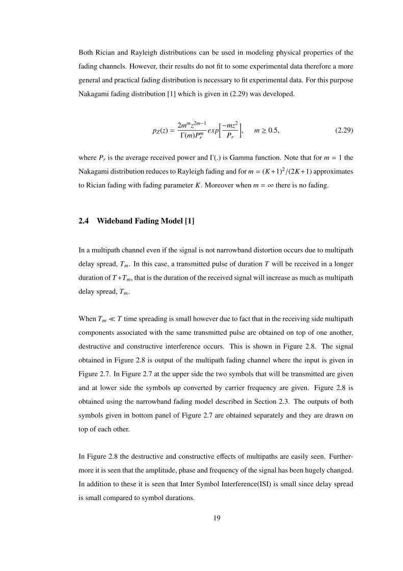
Both Rician and Rayleigh distributions can be used in modeling physical properties of the
fading channels. However, their results do not fit to some experimental data therefore a more
general and practical fading distribution is necessary to fit experimental data. For this purpose
Nakagami fading distribution [1] which is given in (2.29) was developed.
pZ(z) =2mmz2m−1
Γ(m)Pmr
exp[−mz2
Pr
], m ≥ 0.5, (2.29)
where Pr is the average received power and Γ(.) is Gamma function. Note that for m = 1 the
Nakagami distribution reduces to Rayleigh fading and for m = (K+1)2/(2K+1) approximates
to Rician fading with fading parameter K. Moreover when m = ∞ there is no fading.
2.4 Wideband Fading Model [1]
In a multipath channel even if the signal is not narrowband distortion occurs due to multipath
delay spread, Tm. In this case, a transmitted pulse of duration T will be received in a longer
duration of T +Tm, that is the duration of the received signal will increase as much as multipath
delay spread, Tm.
When Tm � T time spreading is small however due to fact that in the receiving side multipath
components associated with the same transmitted pulse are obtained on top of one another,
destructive and constructive interference occurs. This is shown in Figure 2.8. The signal
obtained in Figure 2.8 is output of the multipath fading channel where the input is given in
Figure 2.7. In Figure 2.7 at the upper side the two symbols that will be transmitted are given
and at lower side the symbols up converted by carrier frequency are given. Figure 2.8 is
obtained using the narrowband fading model described in Section 2.3. The outputs of both
symbols given in bottom panel of Figure 2.7 are obtained separately and they are drawn on
top of each other.
In Figure 2.8 the destructive and constructive effects of multipaths are easily seen. Further-
more it is seen that the amplitude, phase and frequency of the signal has been hugely changed.
In addition to these it is seen that Inter Symbol Interference(ISI) is small since delay spread
is small compared to symbol durations.
19
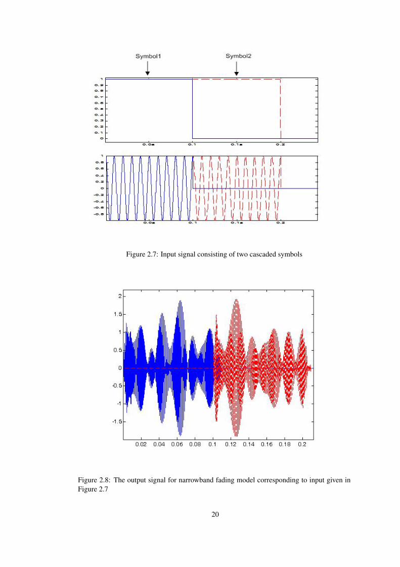
Figure 2.7: Input signal consisting of two cascaded symbols
Figure 2.8: The output signal for narrowband fading model corresponding to input given inFigure 2.7
20
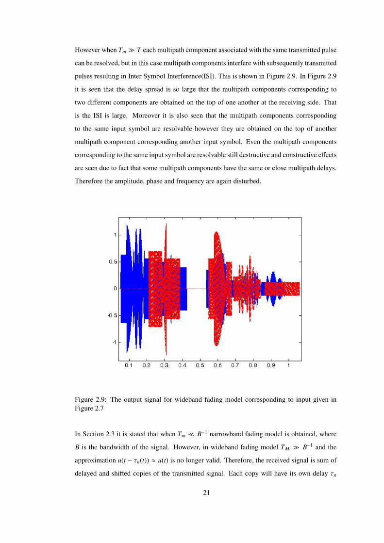
However when Tm � T each multipath component associated with the same transmitted pulse
can be resolved, but in this case multipath components interfere with subsequently transmitted
pulses resulting in Inter Symbol Interference(ISI). This is shown in Figure 2.9. In Figure 2.9
it is seen that the delay spread is so large that the multipath components corresponding to
two different components are obtained on the top of one another at the receiving side. That
is the ISI is large. Moreover it is also seen that the multipath components corresponding
to the same input symbol are resolvable however they are obtained on the top of another
multipath component corresponding another input symbol. Even the multipath components
corresponding to the same input symbol are resolvable still destructive and constructive effects
are seen due to fact that some multipath components have the same or close multipath delays.
Therefore the amplitude, phase and frequency are again disturbed.
Figure 2.9: The output signal for wideband fading model corresponding to input given inFigure 2.7
In Section 2.3 it is stated that when Tm � B−1 narrowband fading model is obtained, where
B is the bandwidth of the signal. However, in wideband fading model TM � B−1 and the
approximation u(t − τn(t)) ≈ u(t) is no longer valid. Therefore, the received signal is sum of
delayed and shifted copies of the transmitted signal. Each copy will have its own delay τn
21
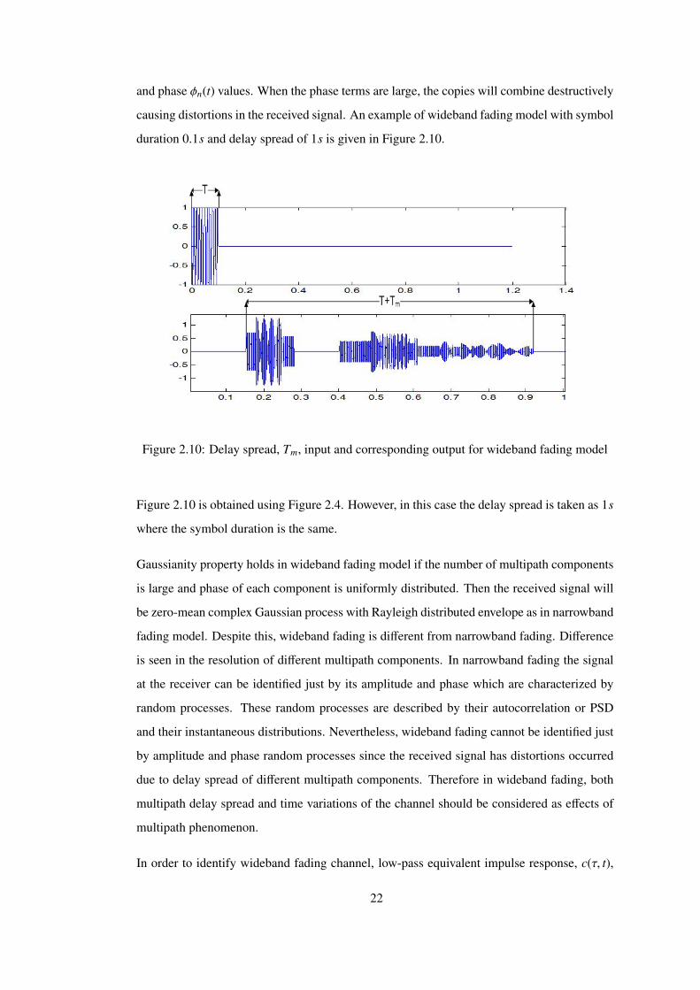
and phase φn(t) values. When the phase terms are large, the copies will combine destructively
causing distortions in the received signal. An example of wideband fading model with symbol
duration 0.1s and delay spread of 1s is given in Figure 2.10.
Figure 2.10: Delay spread, Tm, input and corresponding output for wideband fading model
Figure 2.10 is obtained using Figure 2.4. However, in this case the delay spread is taken as 1s
where the symbol duration is the same.
Gaussianity property holds in wideband fading model if the number of multipath components
is large and phase of each component is uniformly distributed. Then the received signal will
be zero-mean complex Gaussian process with Rayleigh distributed envelope as in narrowband
fading model. Despite this, wideband fading is different from narrowband fading. Difference
is seen in the resolution of different multipath components. In narrowband fading the signal
at the receiver can be identified just by its amplitude and phase which are characterized by
random processes. These random processes are described by their autocorrelation or PSD
and their instantaneous distributions. Nevertheless, wideband fading cannot be identified just
by amplitude and phase random processes since the received signal has distortions occurred
due to delay spread of different multipath components. Therefore in wideband fading, both
multipath delay spread and time variations of the channel should be considered as effects of
multipath phenomenon.
In order to identify wideband fading channel, low-pass equivalent impulse response, c(τ, t),
22
will be investigated. Assuming the impulse response, c(τ, t), as deterministic function of τ
and t, its Fourier transform with respect to t is obtained as follows:
S c(τ, ρ) =
∫ ∞
−∞
c(τ, t)e− j2πρtdt. (2.30)
S c(τ, ρ) is called deterministic scattering function of the low-pass equivalent of the channel
impulse response. Since S c(τ, ρ) is Fourier transform of c(τ, t) with respect to time, it gives
information about Doppler characteristic of the channel by the frequency parameter ρ.
The time-varying channel impulse response c(τ, t) given in (2.6) is generally random not deter-
ministic, since the multipath components have random amplitude, phase, delay and number of
multipath components. So it is characterized statistically. As it was mentioned above if there
are enough number of multipath components c(τ, t) can be assumed to be complex Gaussian
process. Therefore, its statistical properties can be completely determined by its mean, auto-
correlation and cross-correlation of in-phase and quadrature components. It is assumed that
each multipath component has uniformly distributed phase as in narrowband fading model.
Therefore in-phase and quadrature components of c(τ, t) are independent Gaussian processes
with the same autocorrelation, mean of zero and cross-correlation of zero. If the number of
multipath components are small the same characteristics are still true if each multipath com-
ponent has Rayleigh distributed amplitude and uniformly distributed phase. This model holds
when there is not a dominant LOS component.
The autocorrelation function of c(τ, t), which gives its statistical properties is given as follows:
Ac(τ1, τ2; t,∆t) = E[c∗(τ1; t)c(τ2; t + ∆t)]. (2.31)
Here it is assumed that the channel is WSS, that is the autocorrelation function is independent
of time, t, but depends on time difference ∆t. Joint statistic measured at two different times
depends on time difference (in practice most channels are WSS). Thus, (2.31) becomes as
follows:
Ac(τ1, τ2; ∆t) = E[c∗(τ1; t)c(τ2; t + ∆t)]. (2.32)
23
In practice the channel response corresponding to multipath component of delay τ1 is uncor-
related with channel response corresponding to multipath component with different delay τ2,
where τ1 , τ2. This is because they are scattered by different scatterers. Such a channel
has uncorrelated scattering (US). Channels which are both WSS and US are abbreviated as
WSSUS. When US property is included in (2.32), it yields
E[c∗(τ1; t)c(τ2; t + ∆t)] = Ac(τ1; ∆t)δ[τ1 − τ2] , Ac(τ; ∆t). (2.33)
Ac(τ; ∆t) given in (2.33) is the average output power corresponding to channel as a function
of multipath delay τ = τ1 = τ2 and time difference ∆t in observation time. For this function
it is assumed that delay difference is bigger than inverse of bandwidth that is, |τ1 − τ2| > B−1,
in order to resolve two components.
The scattering function for random channels is Fourier transform of Ac(τ; ∆t) with respect
to ∆t and is given as follows:
S c(τ, ρ) =
∫ ∞
−∞
Ac(τ,∆t)e− j2πρ∆td∆t. (2.34)
S c(τ, ρ) identifies average power corresponding to channel as a function of multipath delay τ
and Doppler ρ since it is Fourier transform of Ac(τ,∆t). The most important properties of the
wideband channel is obtained from autocorrelation function Ac(τ,∆t) or scattering function
S c(τ, ρ).
2.4.1 Power Delay Profile
Power delay profile Ac(τ), also called multipath intensity profile is defined as Ac(τ) , Ac(τ, 0).
It is obvious that power delay profile gives average power associated with a given multipath
delay.
If the pdf of random delay spread Tm is defined in terms of Ac(τ) as follows:
pTm =Ac(τ)∫ ∞
0 Ac(τ)dτ, (2.35)
then mean and rms delay spread are defined as follows:
24
µTm =
∫ ∞0 τAc(τ)dτ∫ ∞0 Ac(τ)dτ
(2.36)
σTm =
√√√∫ ∞0 (τ − µTm)2Ac(τ)dτ∫ ∞
0 Ac(τ)dτ(2.37)
where µTm and σTm are mean and rms delay spreads respectively. Defining mean, rms delay
spread or equivalently pdf given in (2.35) in terms of Ac(τ) means that the delay associated
with a given multipath component is related to its power. Therefore the multipath components
with small power contributes less to delay spread. In general the multipath components which
are below noise floor are not used for calculation of multipath delay spread.
In general a delay T where Ac(τ) ≈ 0 for τ ≥ T can be used for the delay spread of the channel
and this value is taken as integer multiple of rms delay spread, that is T = 3σTm . Under this
approximation, Ac(τ) ≈ 0 for τ > 3σTm , a linearly modulated signal with symbol period Ts can
have or not have ISI depending on the relation between Ts and σTm . If Ts � σTm(wideband
fading) then the signal will experience a large ISI. In contrast if Ts � σTm(narrowband fading)
then the signal will experience negligible ISI. Finally when Ts is on the order ofσTm then there
will be some ISI which may or may not decrease the performance of the system depending
on the properties of the system and channel.
The relationship between µTm and σTm depends on the shape of Ac(τ), but in general µTm ≈
σTm . If there is no LOS component and small number of multipath components with nearly
the same delays in the channel then µTm � σTm .
2.4.2 Coherence Bandwidth
Time varying multipath random channel can also be characterized by taking Fourier transform
of the channel impulse response c(τ, t) with respect to τ, that is it will be investigated in the
frequency domain. Thus,
C( f ; t) =
∫ ∞
−∞
c(τ, t)e− j2π f τdτ. (2.38)
25
It is known that c(τ, t) is WSS and is a complex zero-mean Gaussian random variable in t,
therefore C( f ; t) is also WSS and zero-mean complex Gaussian random process since it is the
integral of c(τ, t) and (2.38) represents the sum of complex zero-mean Gaussian processes.
Therefore C( f ; t) can be characterized by its autocorrelation function which is given as:
AC( f1, f2; ∆t) = E[C∗( f1; t)C( f2; t + ∆t)]. (2.39)
AC( f1, f2; ∆t) can be simplified as follows :
AC( f1, f2; ∆t) = E[ ∫ ∞
−∞
c∗(τ1; t)e j2π f1τ1dτ1
∫ ∞
−∞
c(τ2; t + ∆t)e− j2π f2τ2dτ2
]= AC(∆ f ; ∆t), (2.40)
where ∆ f = f1− f2 and the equality is obtained by the help of WSS and US property of c(τ; t).
If ∆t is taken zero in (2.40) then Fourier transform of the power delay profile, Ac(τ) is obtained
which is defined as AC(∆ f ) , AC(∆ f ; 0) and is given as follows
AC(∆ f ) =
∫ ∞
−∞
Ac(τ)e− j2π f τdτ. (2.41)
AC(∆ f ) can also be shown to be AC(∆ f ) = E[C∗( f ; t)C( f + ∆ f ; t), that is it is an autocor-
relation function. Then the channel response is independent at approximately ∆ f frequency
separations where AC(∆ f ) ≈ 0. The frequency Bc is called the coherence bandwidth of the
channel where AC(∆ f ) ≈ 0 for all ∆ f > Bc. By the Fourier transform relation it is obvious
that when Ac(τ) ≈ 0 for τ > T then AC(∆ f ) ≈ 0 for ∆ f > 1/T . Therefore, the coherence
bandwidth Bc can be approximated as Bc ≈ 1/T , where T is generally taken as RMS delay
spread, σTm , of Ac(τ). A more general approximation can be made as Bc ≈ k/σTm where k
depends on the shape of Ac(τ) and exact definition of coherence bandwidth.
According to the signal bandwidth transmitted, the fading can be flat (frequency non-selective)
or frequency-selective. If the bandwidth of the transmitted signal B is B << Bc then the fad-
ing is nearly equal for all signal bandwidth, that is it is highly correlated. In this case flat
fading is obtained. In linear modulation the signal bandwidth is inversely proportional to
26
symbol time Ts. Therefore for flat fading it means that Ts ≈ 1/B >> 1/Bc = σTm , that is there
is negligible ISI in the channel. Conversely if B is B >> Bc then frequency selective fading
is obtained. In this case the channel amplitude through the signal bandwidth is highly chang-
ing this is because the channel amplitude value at frequencies separated more than coherence
bandwidth are roughly independent. In frequency selective fading Ts ≈ 1/B << 1/Bc = σTm ,
that is there is large ISI in the channel. A plot of Ac(τ) and its Fourier transform AC(∆ f ) with
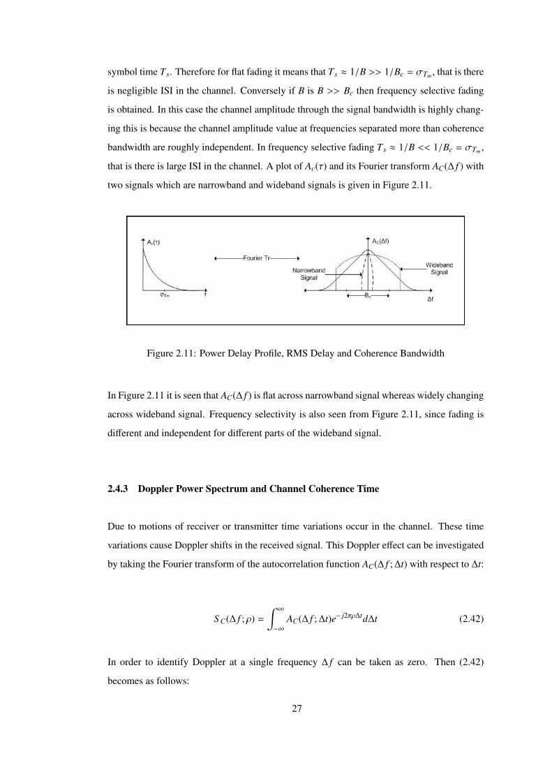
two signals which are narrowband and wideband signals is given in Figure 2.11.
Figure 2.11: Power Delay Profile, RMS Delay and Coherence Bandwidth
In Figure 2.11 it is seen that AC(∆ f ) is flat across narrowband signal whereas widely changing
across wideband signal. Frequency selectivity is also seen from Figure 2.11, since fading is
different and independent for different parts of the wideband signal.
2.4.3 Doppler Power Spectrum and Channel Coherence Time
Due to motions of receiver or transmitter time variations occur in the channel. These time
variations cause Doppler shifts in the received signal. This Doppler effect can be investigated
by taking the Fourier transform of the autocorrelation function AC(∆ f ; ∆t) with respect to ∆t:
S C(∆ f ; ρ) =
∫ ∞
−∞
AC(∆ f ; ∆t)e− j2πρ∆td∆t (2.42)
In order to identify Doppler at a single frequency ∆ f can be taken as zero. Then (2.42)
becomes as follows:
27
S C(ρ) =
∫ ∞
−∞
AC(∆t)e− j2πρ∆td∆t, (2.43)
where AC(∆t) , AC(∆ f = 0; ∆t) is the autocorrelation function which gives information
about how channel impulse response decorrelates over time.
Specifically, when AC(∆t = T ) = 0 is satisfied, observations of the channel impulse response
separated by T are uncorrelated and so independent since the channel impulse response is
Gaussian random process. Channel coherence time, Tc is defined to be the range over
which AC(∆t) is nonzero. Therefore it can be said that time varying channel decorrelates
after approximately Tc seconds. S C(ρ) given in (2.43) is called Doppler power spectrum
of the channel and gives PSD of the received signal as a function of Doppler ρ, since it is
Fourier transform of autocorrelation function AC(∆t). The maximum ρ value for which S C(ρ)
is approximately nonzero is called Doppler spread and is shown by BD. Using the Fourier
transform relationship between AC(∆t) and S C(ρ), it is obtained that BD ≈ 1/Tc. In general
BD ≈ k/Tc where k depends on the shape of S C(ρ). A plot of Doppler power spectrum and its
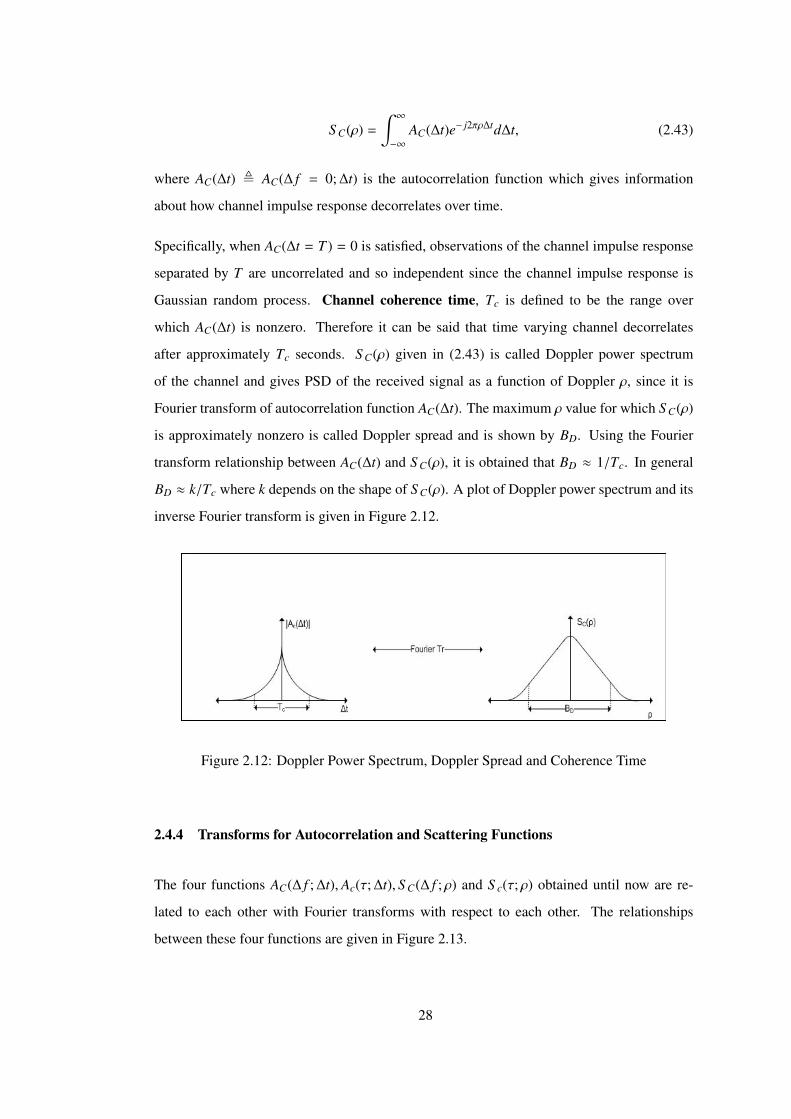
inverse Fourier transform is given in Figure 2.12.
Figure 2.12: Doppler Power Spectrum, Doppler Spread and Coherence Time
2.4.4 Transforms for Autocorrelation and Scattering Functions
The four functions AC(∆ f ; ∆t), Ac(τ; ∆t), S C(∆ f ; ρ) and S c(τ; ρ) obtained until now are re-
lated to each other with Fourier transforms with respect to each other. The relationships
between these four functions are given in Figure 2.13.
28
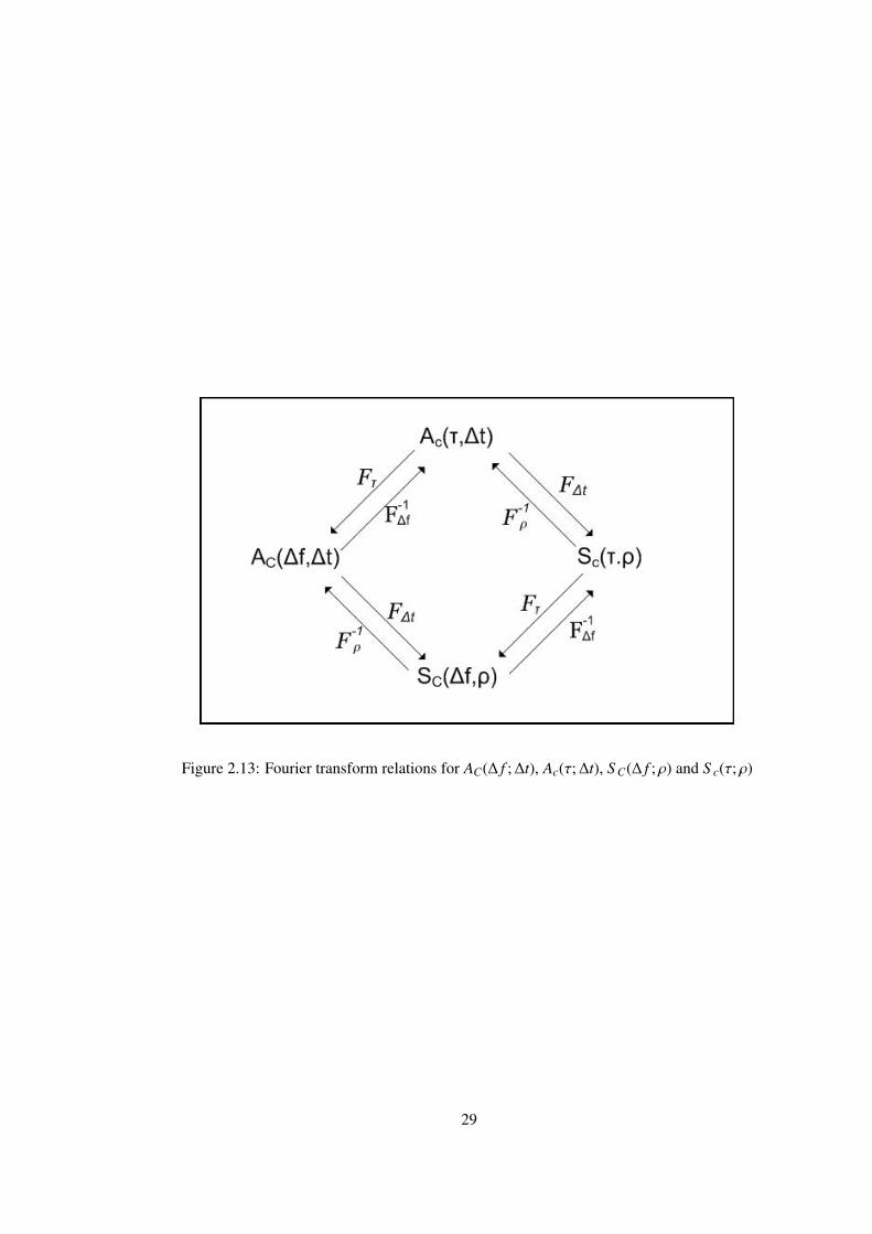
Figure 2.13: Fourier transform relations for AC(∆ f ; ∆t), Ac(τ; ∆t), S C(∆ f ; ρ) and S c(τ; ρ)
29
CHAPTER 3
UNDERWATER ACOUSTIC CHANNEL
The channel model given in Chapter 2 is a general multipath fading channel for electromag-
netic waves in air. Underwater acoustic channel (UAC) can also be modeled as a multipath
fading channel. However, there is not a standardized model proposed for underwater acoustic
channel fading for the moment and experimental studies are conducted to determine the sta-
tistical properties of underwater acoustic channel [4]. There are basic differences in between
wireless channels in air and in underwater. The attenuation increases as frequency increases
in underwater channels. The existence of surface and bottom layers limits the propagation of
acoustic signals and greatly increases the multipath effects. The rapid fluctuations resulted
from surface waves decreases coherence time of underwater channel. The speed of the acous-
tic signal in underwater environment is smaller compared to electromagnetic signals in air and
it is comparable with the speed of the receiver and the transmitter . Therefore, the Doppler
effect is larger in underwater channels.
Underwater acoustic channel (UAC) is one of the most difficult channels for data transmis-
sion, communication and signal processing. Difficulty of the media comes from its complex,
dynamic and unpredictable nature. Underwater channel may quickly change by environmen-
tal and biological conditions. The underwater channel’s behavior is best characterized with
extremely unpredictable and varying multipath, very large propagation delays, attenuation
of signals increasing with distance and frequency, low and limited bandwidth, time variable
physical conditions, noise, low and varying speed of sound, high Doppler spread, time vary-
ing Doppler shift and ambient interference. These phenomena can significantly damage signal
as it propagates through the channel. Therefore in order to get a reliable channel model for
underwater signal processing the factors mentioned above should be accounted for. The prop-
30
agation of an acoustic signal in underwater channel is best succeeded in low frequencies due
to the fact that the attenuation of the acoustic signal increases as its frequency increases. The
bandwidth of the channel is severely limited and is distance dependent. Although the band-
width is low, underwater systems are actually wideband since the bandwidth of the channel
is not negligible compared to center frequency. In underwater channel the received signal has
greater bandwidth and time duration than transmitted signal, such channels are called spread
channels. Spread channels can be represented by a time-varying impulse response c(τ, t) [11]
where t is time and τ is delay.
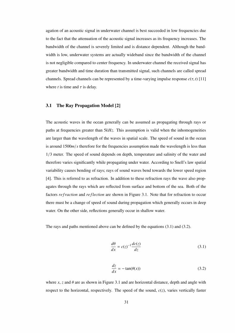
3.1 The Ray Propagation Model [2]
The acoustic waves in the ocean generally can be assumed as propagating through rays or
paths at frequencies greater than 5kHz. This assumption is valid when the inhomogeneities
are larger than the wavelength of the waves in spatial scale. The speed of sound in the ocean
is around 1500m/s therefore for the frequencies assumption made the wavelength is less than
1/3 meter. The speed of sound depends on depth, temperature and salinity of the water and
therefore varies significantly while propagating under water. According to Snell’s law spatial
variability causes bending of rays; rays of sound waves bend towards the lower speed region
[4]. This is referred to as refraction. In addition to these refraction rays the wave also prop-
agates through the rays which are reflected from surface and bottom of the sea. Both of the
factors re f raction and re f lection are shown in Figure 3.1. Note that for refraction to occur
there must be a change of speed of sound during propagation which generally occurs in deep
water. On the other side, reflections generally occur in shallow water.
The rays and paths mentioned above can be defined by the equations (3.1) and (3.2).
dθdx
= c(z)−1 dc(z)dz
(3.1)
dzdx
= − tan(θ(x)) (3.2)
where x, z and θ are as shown in Figure 3.1 and are horizontal distance, depth and angle with
respect to the horizontal, respectively. The speed of the sound, c(z), varies vertically faster
31
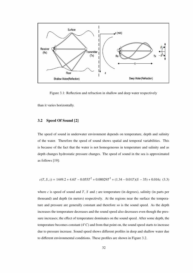
Figure 3.1: Reflection and refraction in shallow and deep water respectively
than it varies horizontally.
3.2 Speed Of Sound [2]
The speed of sound in underwater environment depends on temperature, depth and salinity
of the water. Therefore the speed of sound shows spatial and temporal variabilities. This
is because of the fact that the water is not homogeneous in temperature and salinity and as
depth changes hydrostatic pressure changes. The speed of sound in the sea is approximated
as follows [19]:
c(T, S , z) = 1449.2 + 4.6T − 0.055T 2 + 0.00029T 3 + (1.34 − 0.01T )(S − 35) + 0.016z (3.3)
where c is speed of sound and T , S and z are temperature (in degrees), salinity (in parts per
thousand) and depth (in meters) respectively. At the regions near the surface the tempera-
ture and pressure are generally constant and therefore so is the sound speed. As the depth
increases the temperature decreases and the sound speed also decreases even though the pres-
sure increases; the effect of temperature dominates on the sound speed. After some depth, the
temperature becomes constant (4◦C) and from that point on, the sound speed starts to increase
due to pressure increase. Sound speed shows different profiles in deep and shallow water due
to different environmental conditions. These profiles are shown in Figure 3.2.
32
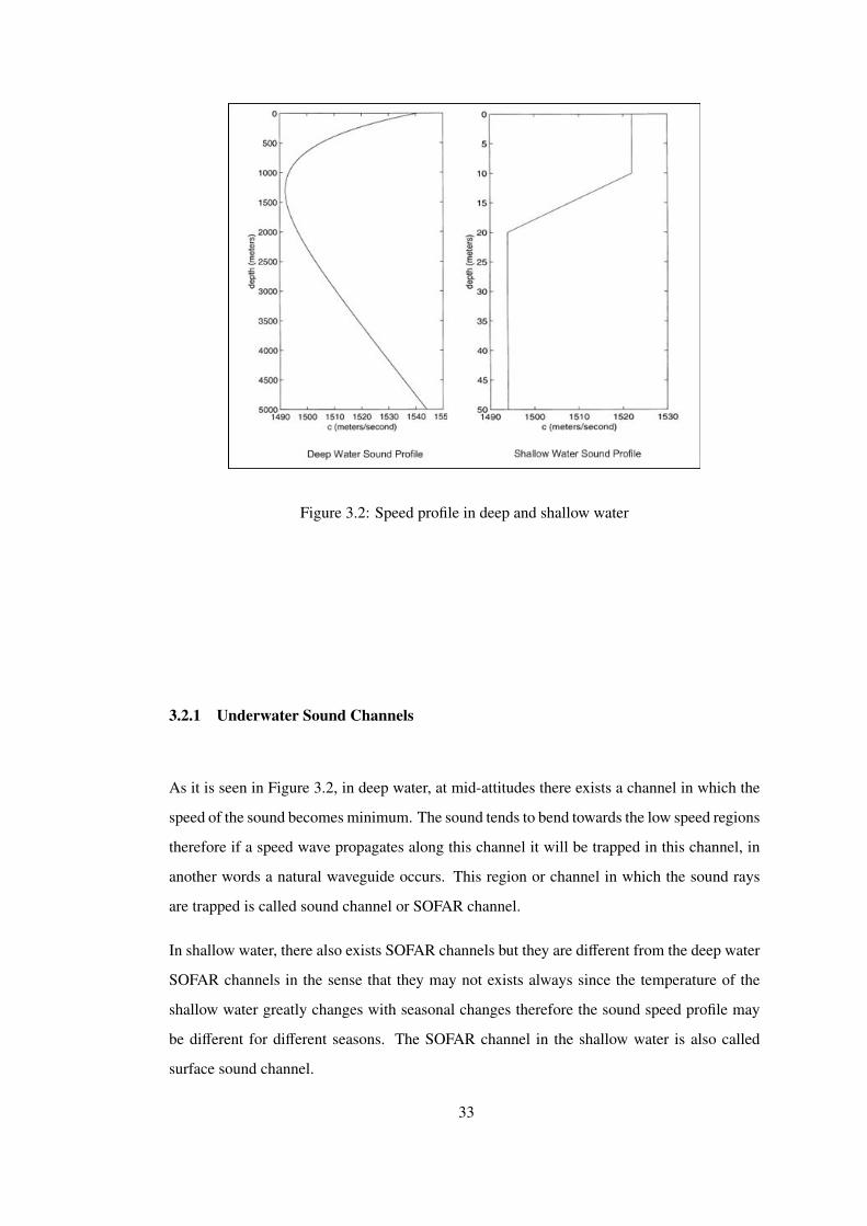
Figure 3.2: Speed profile in deep and shallow water
3.2.1 Underwater Sound Channels
As it is seen in Figure 3.2, in deep water, at mid-attitudes there exists a channel in which the
speed of the sound becomes minimum. The sound tends to bend towards the low speed regions
therefore if a speed wave propagates along this channel it will be trapped in this channel, in
another words a natural waveguide occurs. This region or channel in which the sound rays
are trapped is called sound channel or SOFAR channel.
In shallow water, there also exists SOFAR channels but they are different from the deep water
SOFAR channels in the sense that they may not exists always since the temperature of the
shallow water greatly changes with seasonal changes therefore the sound speed profile may
be different for different seasons. The SOFAR channel in the shallow water is also called
surface sound channel.
33
3.3 Attenuation and Noise
In an underwater acoustic channel, the energy of the transmitted signal is partly transferred
to heat energy. In addition to that some parts of the energy is lost during scatterings from the
surface and bottom. In an underwater acoustic channel the loss mechanisms are spreading
loss, absorption loss and scattering loss.
3.3.1 Spreading Loss
The spreading loss is seen in two types; spherical loss for deep water and cylindrical loss
for shallow water [20]. Actually, the spherical and cylindrical loss is categorized according
to the distance from the source point. If the vertical propagation has reached to its limit
imposed by sea floor and sea surface then from that point on cylindrical propagation starts
for horizontal propagation. In spherical loss the attenuation of the signal is proportional to
inverse square of the distance from source point (1/r2, where r is distance from the source)
and for cylindrical loss it is proportional to inverse of distance from the source point (1/r).
Therefore the spreading loss for a distance r from source point is given by (3.4).
Ls = rk (3.4)
In (3.4), k is energy spreading factor and it is 2 for spherical, 1 for cylindrical and 1.5 for
practical spreading [21].
3.3.2 Absorption Loss
In an acoustic channel one of the most important distinguishing property is the fact that the
path loss depends on signal’s frequency. The reason for that fact is the transfer of acoustic
energy to the heat energy, that is absorption loss. Absorption loss can be approximated as
follows:
La = ar (3.5)
34
where r is the distance from the source point and a is the frequency dependent term which is
given as [21]:
a = 10α( f )/10 (3.6)
The term α( f ) in (3.6) is the absorption coefficient [19]:
α( f ) = 0.11f 2
1 + f 2 + 44f 2
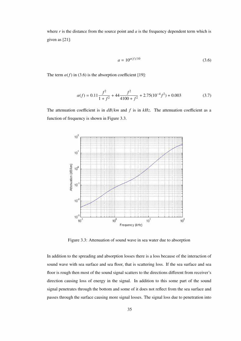
4100 + f 2 + 2.75(10−4 f 2) + 0.003 (3.7)
The attenuation coefficient is in dB/km and f is in kHz. The attenuation coefficient as a
function of frequency is shown in Figure 3.3.
Figure 3.3: Attenuation of sound wave in sea water due to absorption
In addition to the spreading and absorption losses there is a loss because of the interaction of
sound wave with sea surface and sea floor, that is scattering loss. If the sea surface and sea
floor is rough then most of the sound signal scatters to the directions different from receiver’s
direction causing loss of energy in the signal. In addition to this some part of the sound
signal penetrates through the bottom and some of it does not reflect from the sea surface and
passes through the surface causing more signal losses. The signal loss due to penetration into
35
the bottom is greatly higher then absorption through the water. The loss due to surface and
bottom scattering increases as grazing angle of the sound increases. Moreover, for bottom
scattering case the loss greatly depends on the type of the bottom.
In deep water, existence of SOFAR channel causes the sound wave to propagate without
interacting with bottom and surface. This decreases the amount of loss and therefore increases
the amount of distance that the sound wave can travel. In SOFAR channel, the only sources of
loss are spreading and absorption loss by the water. Therefore it can be said that the effective
range over which sound can travel is larger in deep water than that in shallow water.
Ignoring the loss due to interaction with surface and bottom, scattering loss and fading effect
due to multipath, the signal level (S L in dB) at a distance r from the source can be obtained
as follows [2]:
S L = 169 + 10log10(P) − αr − 20log10(d/2) − 10log10(r − d/2) (3.8)
where P is the power of the radiated signal in watts, α is the absorption coefficient, r is the
distance from the source point and d is the depth of the water and the constant term 169 comes
from conversion of electric power to acoustic power. In (3.8) it is assumed that the transducer
is omni-directional and the depth of the water is smaller than the distance from the source,
that is d < r. Moreover, the first two terms in (3.8) are due to signal power, the other terms
are due to absorption loss, spherical loss and cylindrical loss respectively. Note that here the
total loss is the combination of spreading loss and absorption loss which is given as:
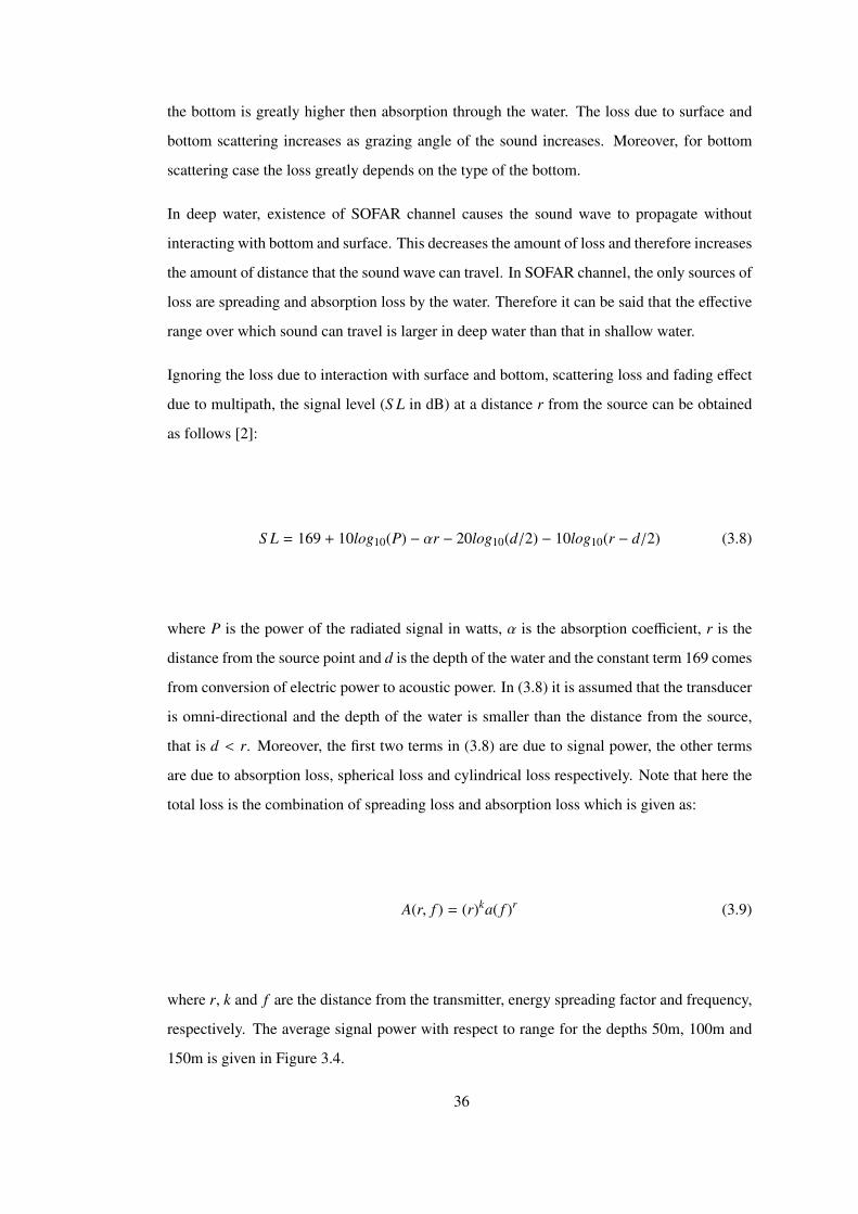
A(r, f ) = (r)ka( f )r (3.9)
where r, k and f are the distance from the transmitter, energy spreading factor and frequency,
respectively. The average signal power with respect to range for the depths 50m, 100m and
150m is given in Figure 3.4.
36
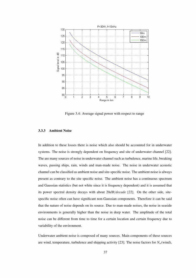
Figure 3.4: Average signal power with respect to range
3.3.3 Ambient Noise
In addition to these losses there is noise which also should be accounted for in underwater
systems. The noise is strongly dependent on frequency and site of underwater channel [22].
The are many sources of noise in underwater channel such as turbulence, marine life, breaking
waves, passing ships, rain, winds and man-made noise. The noise in underwater acoustic
channel can be classified as ambient noise and site-specific noise. The ambient noise is always
present as contrary to the site specific noise. The ambient noise has a continuous spectrum
and Gaussian statistics (but not white since it is frequency dependent) and it is assumed that
its power spectral density decays with about 20dB/decade [22]. On the other side, site-
specific noise often can have significant non-Gaussian components. Therefore it can be said
that the nature of noise depends on its source. Due to man-made noises, the noise in seaside
environments is generally higher than the noise in deep water. The amplitude of the total
noise can be different from time to time for a certain location and certain frequency due to
variability of the environment.
Underwater ambient noise is composed of many sources. Main components of these sources
are wind, temperature, turbulence and shipping activity [23]. The noise factors for Nw(wind),
37
Nte(temperature), Ntu(turbulence) and Ns(shipping activity) are given in dB re µPa as follows:
10log10(Nw( f )) = 50 + 7.5w0.5 + 20log10( f ) − 40log10( f + 0.4) dB re µPa (3.10)
10log10(Nte( f )) = −15 + 20log10( f ) dB re µPa (3.11)
10log10(Ntu( f )) = 17 − 30log10( f ) dB re µPa (3.12)
10log10(Ns( f )) = 40 + 20(s − 0.5) + 26log10( f ) − 60log10( f + 0.03) dB re µPa (3.13)
where w is wind speed in m/s, s is the shipping activity and f is in kHz. The shipping activity
lies between 0(no activity) and 1(maximum activity). The re abbreviation given in units of
noises given in (3.13) stands for relative. Therefore, the values of noises given in (3.13) are
relative to 1µPa in dB scale. The total ambient noise is obtained as
N( f ) = Nw( f ) + Nte( f ) + Ntu( f ) + Ns( f ). (3.14)
The power spectral density of the total noise given in (3.14) is shown in Figure 3.5. The most
important factor of the total noise in the range 100Hz < f < 100kHz is the wind speed. This
range is usually operating region for most of the underwater acoustic systems.
As it is mentioned above the attenuation increases as frequency increases and and as the
propagation range increases. Therefore the SNR on the receiver side is a function of frequency
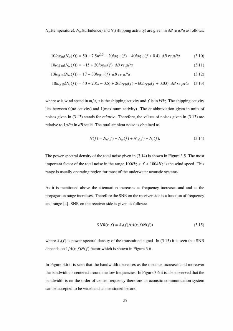
and range [4]. SNR on the receiver side is given as follows:
S NR(r, f ) = S t( f )/(A(r, f )N( f )) (3.15)
where S t( f ) is power spectral density of the transmitted signal. In (3.15) it is seen that SNR
depends on 1/A(r, f )N( f ) factor which is shown in Figure 3.6.
In Figure 3.6 it is seen that the bandwidth decreases as the distance increases and moreover
the bandwidth is centered around the low frequencies. In Figure 3.6 it is also observed that the
bandwidth is on the order of center frequency therefore an acoustic communication system
can be accepted to be wideband as mentioned before.
38

Figure 3.5: Noise Power Spectral Density for ship activity=0 and wind speed=0, 5, 10 m/s.
Figure 3.6: SNR depends on frequency and distance by the factor 1/A(r,f)N(f)
39
3.4 Multipath [2, 3, 4]
Propagation of the acoustic signal occurs over multiple paths, therefore at the receiver side,
multiple of transmitted signal with different amplitude, delay and phase are observed. This
multipath phenomena causes distortion in the received signal since the received multipath
signals interfere with each other. The multipath formation is result of reflection or refraction.
The reflection and scattering of acoustic signal can be from the surface, bottom and any ob-
jects in the channel, in addition to that multipath can occur due to sound refraction in water.
Sound refraction is a consequence of sound speed variation with depth, which is generally
seen in deep water environment. The two formations of multipath in shallow and deep water
are shown in Figure 3.1. The number of paths due to refraction changes due to environmental
conditions such as pressure, temperature and density since the speed of sound depends on
these factors [4]. In addition to that the number of multipaths depend on the geometry and
physical properties of the channel therefore the channel impulse response differs from loca-
tion to location even from time to time for the same location. The interference caused by
multipath is time-varying and can be in such levels that the amplitude of the received signal
can increase and decrease significantly in another word fades. The variability of the multipath
is due to variability of the channel caused by temporal fluctuations such as internal and surface
waves, turbulence, tidal flows and platform motion [2]. In a real underwater channel there can
be infinitely many paths, however the ones that are below the noise level are ignored. Each
path between the transmitter and receiver has its own spreading The total multipath spread is
determined by the longest path or last arrived path.
The channel response can be obtained by adding all responses of multipaths which have dif-
ferent amplitudes, phases and delays. For a single path the channel response depends on the
path length and frequency, since the arrival time and path loss depend on these variables.
3.4.1 Micro- and Macro-Multipath
The micro and macro multipaths are classified according to sources of their formation. The
paths that are formed by slowly varying characteristic of the ocean are called macro-multipaths
and the paths that are formed by rapidly varying characteristic of the ocean are called micro-
multipaths. Therefore the channel is decomposed in two parts, the slowly varying, half-
40
deterministic part and rapidly varying, stochastic part [2].
Assuming that only first part of the ocean(half-deterministic part) is available and that the
ocean surface is flat and the floor has only large scale features, the received signal’s portion
for a transmitted signal of e jωt in the lth path is given in (3.16). Here the large-scale or small
scale terms are determined according to the spatial scales compared to acoustical wavelength.
If a factor is bigger than the acoustical wavelength in spatial scale then it is large-scale or vice
versa.
Rl(t, ω) = Hl(t, ω)e jωt. (3.16)
In (3.16) the function Hl(ω, t) is complex-valued and depends on slowly varying changes,
speed of sound, large scale features of the sea floor and positions of the receiver and transmit-
ter. Since Rl(t, ω) is the signal part which propagates along the lth path, Hl(ω, t) represents
slowly varying phase delay and loss of the signal on that path only. The solid lines shown in
Figure 3.1 construct macro-multipaths structure of the channel and are formed under the as-
sumptions made above. The sound would not have to propagate along solid lines in Figure 3.1
if the assumptions made above are removed. In this situation the sound would be reflected and
scattered from the small scale features of the ocean. Then the sound will propagate through
a ray tube surrounding the rays defined by macro-multipath structure. These ray tubes are
shown in Figure 3.1 as gray regions surrounding the solid lines.
If the fluctuations in the ocean have small amplitude or large spatial scale then the sound will
propagate in the ray tube as a single disturbed path. This single path is divided into many
micro paths in the ray tube as fluctuations’ amplitude increases or their scale decreases. In
this case the total portion of the received signal propagating in the lth ray tube is the sum of
all micro paths in the lth ray tube. These micro paths constitute micro-multipath structure of
the channel. Including the effects of rapid fluctuations and small scale environmental factors
the portion of the received signal in the lth ray is obtained as follows:
Rl(t, ω) = Ψl(t, ω)Rl(t, ω) = Ψl(t, ω)Hl(t, ω)e jωt (3.17)
where Ψl(t, ω) accounts for the effects of micro-multipath structure.
41
Assuming total of L rays between the transmitter and receiver the received signal, R(t, ω), for
the transmitted signal of e jωt is obtained as follows:
R(t, ω) =
L∑l=1
Rl(t, ω). (3.18)
Rays between the transmitter and receiver generally do not overlap or have little overlap,
thus unless the scale of the environmental fluctuations is on the order of rays’ separation, the
correlation between signal fluctuations due to micro-multipath in different rays is small.
The channel between the transmitter and receiver can also be characterized by using input
delay spread function, g(t, τ). For this case the relationship between input and output is given
as follows [2]:
r(t) =
∫ ∞
−∞
g(t, τ)s(t − τ)dτ, (3.19)
where s(t) is input and r(t) is the output of the channel. In (3.19) it is seen that when input
delay spread is not function of time then g(t, τ) reduces to time invariant impulse response. Let
R(ω) = G(t, ω)S (ω) be the Fourier transform of the received signal where G(t, ω) and S (ω)
are Fourier transforms of the input delay spread function and transmitted signal respectively.
Then it can be easily shown that:
r(t) =1
2π
∫ ∞
−∞
G(t, ω)S (ω)e jωtdω. (3.20)
Using linearity of the channel and (3.18) it can be shown that for the lth ray tube the received
signal portion rl(t) is obtained as follows:
rl(t) =1
2π
∫ ∞
−∞
Gl(t, ω)S (ω)e jωtdω. (3.21)
Comparing (3.21) and (3.17) it is seen that Gl(t, ω) = Ψl(t, ω)Hl(t, ω). Therefore the input
delay spread function of the lth ray tube using inverse Fourier transform is obtained as follows:
gl(t, τ) =1
2π
∫ ∞
−∞
Gl(t, ω)e jωtdω =1
2π
∫ ∞
−∞
Ψl(t, ω)Hl(t, ω)e jωtdω. (3.22)
42
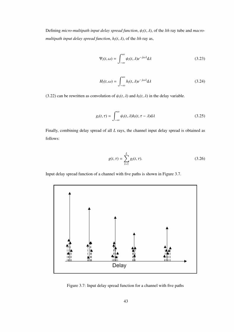
Defining micro-multipath input delay spread function, ψl(t, λ), of the lth ray tube and macro-
multipath input delay spread function, hl(t, λ), of the lth ray as,
Ψl(t, ω) =
∫ ∞
−∞
ψl(t, λ)e− jωλdλ (3.23)
Hl(t, ω) =
∫ ∞
−∞
hl(t, λ)e− jωλdλ (3.24)
(3.22) can be rewritten as convolution of ψl(t, λ) and hl(t, λ) in the delay variable.
gl(t, τ) =
∫ ∞
−∞
ψl(t, λ)hl(t, τ − λ)dλ (3.25)
Finally, combining delay spread of all L rays, the channel input delay spread is obtained as
follows:
g(t, τ) =
L∑l=1
gl(t, τ). (3.26)
Input delay spread function of a channel with five paths is shown in Figure 3.7.
Figure 3.7: Input delay spread function for a channel with five paths
43
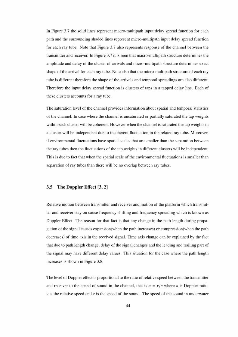
In Figure 3.7 the solid lines represent macro-multipath input delay spread function for each
path and the surrounding shaded lines represent micro-multipath input delay spread function
for each ray tube. Note that Figure 3.7 also represents response of the channel between the
transmitter and receiver. In Figure 3.7 it is seen that macro-multipath structure determines the
amplitude and delay of the cluster of arrivals and micro-multipath structure determines exact
shape of the arrival for each ray tube. Note also that the micro-multipath structure of each ray
tube is different therefore the shape of the arrivals and temporal spreadings are also different.
Therefore the input delay spread function is clusters of taps in a tapped delay line. Each of
these clusters accounts for a ray tube.
The saturation level of the channel provides information about spatial and temporal statistics
of the channel. In case where the channel is unsaturated or partially saturated the tap weights
within each cluster will be coherent. However when the channel is saturated the tap weights in
a cluster will be independent due to incoherent fluctuation in the related ray tube. Moreover,
if environmental fluctuations have spatial scales that are smaller than the separation between
the ray tubes then the fluctuations of the tap weights in different clusters will be independent.
This is due to fact that when the spatial scale of the environmental fluctuations is smaller than
separation of ray tubes than there will be no overlap between ray tubes.
3.5 The Doppler Effect [3, 2]
Relative motion between transmitter and receiver and motion of the platform which transmit-
ter and receiver stay on cause frequency shifting and frequency spreading which is known as
Doppler Effect. The reason for that fact is that any change in the path length during propa-
gation of the signal causes expansion(when the path increases) or compression(when the path
decreases) of time axis in the received signal. Time axis change can be explained by the fact
that due to path length change, delay of the signal changes and the leading and trailing part of
the signal may have different delay values. This situation for the case where the path length
increases is shown in Figure 3.8.
The level of Doppler effect is proportional to the ratio of relative speed between the transmitter
and receiver to the speed of sound in the channel, that is a = v/c where a is Doppler ratio,
v is the relative speed and c is the speed of the sound. The speed of the sound in underwater
44
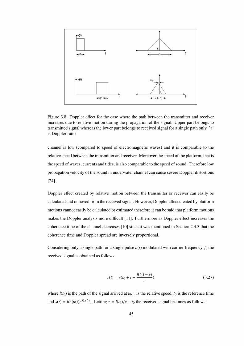
Figure 3.8: Doppler effect for the case where the path between the transmitter and receiverincreases due to relative motion during the propagation of the signal. Upper part belongs totransmitted signal whereas the lower part belongs to received signal for a single path only. ’a’is Doppler ratio
channel is low (compared to speed of electromagnetic waves) and it is comparable to the
relative speed between the transmitter and receiver. Moreover the speed of the platform, that is
the speed of waves, currents and tides, is also comparable to the speed of sound. Therefore low
propagation velocity of the sound in underwater channel can cause severe Doppler distortions
[24].
Doppler effect created by relative motion between the transmitter or receiver can easily be
calculated and removed from the received signal. However, Doppler effect created by platform
motions cannot easily be calculated or estimated therefore it can be said that platform motions
makes the Doppler analysis more difficult [11]. Furthermore as Doppler effect increases the
coherence time of the channel decreases [10] since it was mentioned in Section 2.4.3 that the
coherence time and Doppler spread are inversely proportional.
Considering only a single path for a single pulse u(t) modulated with carrier frequency fc the
received signal is obtained as follows:
r(t) = s(t0 + t −l(t0) − vt
c) (3.27)
where l(t0) is the path of the signal arrived at t0, v is the relative speed, t0 is the reference time
and s(t) = Re{u(t)e j2π fct}. Letting τ = l(t0)/c − t0 the received signal becomes as follows:
45
r(t) = s(t + at − τ) = Re{u(t + at − τ)e j2π fc(t+at−τ)}
= Re{u(t + at − τ)e j2π fc(t+at)e− j2π fcτ}. (3.28)
In (3.28) it is seen that a phase of e− j2π fcτ has been added to the signal. Furthermore it is
observed that the signal has been distorted in two ways. Firstly it has been scaled with (1 + a)
in time. This effect has been illustrated in Figure 3.8. In Figure 3.8 the signal duration has
changed to T/(1 + a) from T . Secondly a frequency offset of a fc has been added. The first
distortion is referred to as Doppler spreading whereas the second one is referred as Doppler
shifting [3]. Doppler shift is also referred to as the mean of frequency shift of the signal over
some window of time [2]. If the mean is removed the remaining frequency fluctuations are
Doppler spread. Doppler shift can be negative (a < 0) or positive (a > 0) according to the
relative motion between the transmitter and receiver. If they get closer to each other positive
Doppler shift(a > 0) is observed, however, if they get away from each other then negative
Doppler shift is observed (a < 0). Since each ray tube has a different propagation path the
Doppler shift can be different for different ray tubes.
In a straight-line propagation of the signal the relative speed generally describes the relative
motion between the transmitter and receiver. However in underwater channel this is not valid
since the sound propagates to the receiver after some reflections and refractions in the channel.
The emission angle and arrival angle will be different from each other therefore the Doppler
effect will be different due to motion of transmitter and receiver [16]. Let us consider the
Doppler shift and the Doppler spread for the two situations for a single path. In the first
one the transmitter moves towards the receiver and the receiver and the ocean is assumed to
be fixed. Whereas in the second one the receiver moves away from the transmitter and the
transmitter and the ocean are assumed to be fixed [16].
For the first case Doppler shift is
fd =Vt fcct
cos(α) = at fccos(α) (3.29)
where α is emission angle, Vt is the velocity of the transmitter and ct is the speed of the sound
at the transmitter. The motion of the transmitter creates no frequency spread for a single ray
tube [16]. For the second case the Doppler shift is obtained as follows [16]:
46
fd = −Vr fccr
cos(β) = ar fccos(β) (3.30)
where β is the angle of arrival, Vr is the speed of the receiver and cr is the speed of the sound
at the receiver side. At the receiver side each path or ray tube has different arrival angle
therefore they cause different Doppler shifts. Micro-multipaths in each ray tube also have
different angles of arrival. Assuming the arrival angle of micro-multipaths in the range ±90◦
around β the maximum and minimum Doppler shifts are obtained as follows [16]:
fdmax = −Vr fccr
cos(90 + β) = −ar fccos(90 − β) = −ar fcsin(β) (3.31)
fdmin = −Vr fccr
cos(0) = ar fc. (3.32)
Therefore the frequency spread caused by Doppler shift in a single ray tube is obtained as
| fdmax − fdmin| = |ar fc(1 + sin(β))|. This frequency spread is centered around fc + ar fccos(β),
that is around the frequency of the macro-multipath. Assuming a frequency spread of ocean
Bo centered about the carrier frequency the total frequency spread is obtained as follows:
fspread = Bo + |ar fc(1 + sin(β))|. (3.33)
When both of the transmitter and receiver are moving simultaneously the total Doppler shift
is the sum of Doppler shifts caused by motions of the transmitter and receiver.
In a wideband system each frequency is shifted with different amount therefore the non-
uniform frequency shift occurs.
3.6 Time Variability
There are two main sources of time variability of the underwater channel. First one is the natu-
ral sources and the second one is the motion of the transmitter or receiver. Natural sources can
also be categorized as long term and short term factors. Among the latter ones the most impor-
tant ones are the changes induced by the surface waves and the internal waves. Random signal
47
fluctuations(micro-multipaths) account for the time variability of the channel response. These
random signal fluctuations are associated with each deterministic path (macro-multipath).
The reason for the fact that the most important contributor to time variability is the reflection
of the sound from the waves is that motion of the reflection point results in a large frequency
spread even much larger than that caused by other factors. In addition to that a dispersion of
energy occurs when the reflection point moves. If there were no waves and the surface of the
ocean was flat then the sound was going to reflect without any distortion but just a phase shift
of π [22]. Vertical motion of the ocean surface can be modeled as a zero mean Gaussian ran-
dom variable, where the power spectrum of the random variable will depend only on the speed
of the wind [22]. For a signal with frequency f , arrival angle of θ for a single reflection from
the surface the Doppler spread is (0.0175/c) f w1.5cos(θ) where c is the speed of the sound and
w is speed of wind [22]. Doppler spread decreases as the distance between the transmitter
and receiver increases, since lower frequencies will be used for long distance transmissions,
on the other hand multipath delay spread will increase. However the channel spread factor
which is the product of Doppler and multipath spread is expected to decrease [22]. A time-
varying multipath channel generally is modeled as a tapped delay line. The gains of the taps
are modeled as stochastic processes with certain power spectral densities and distributions.
Moreover the spaces between the taps are taken as the inverse of twice the channel bandwidth
[22]. The underwater acoustic channel are commonly modeled as Rayleigh fading channel
[16, 9, 25]. However there is no single model accepted for underwater acoustic channel. Even
some authors have modeled underwater acoustic channel as a deterministic model [26].
48
CHAPTER 4
SIMULATION OF UNDERWATER CHANNEL
4.1 Introduction
The test and research operations in underwater channel is expensive, time taking and quite
difficult. Therefore a reliable and accurate model of the underwater channel will be very help-
ful for underwater research, test and other purposes. The model should encounter all physical
properties of the underwater channel mentioned in Chapter 3, since identifying the medium
quantities and physical properties of the channel is the most important step in simulation of
the underwater channel. The model will be more reliable and acceptable as it uses more
physical parameters simultaneously.
In this simulation model following parameters will be used as input parameters:
• Depth of the water
• Depth of the transmitter and receiver
• Horizontal distance between the transmitter and receiver,
• Carrier frequency
• Speed of the transmitter and receiver
• Sea state and wind speed
• Roughness of the bottom
• Temperature
49
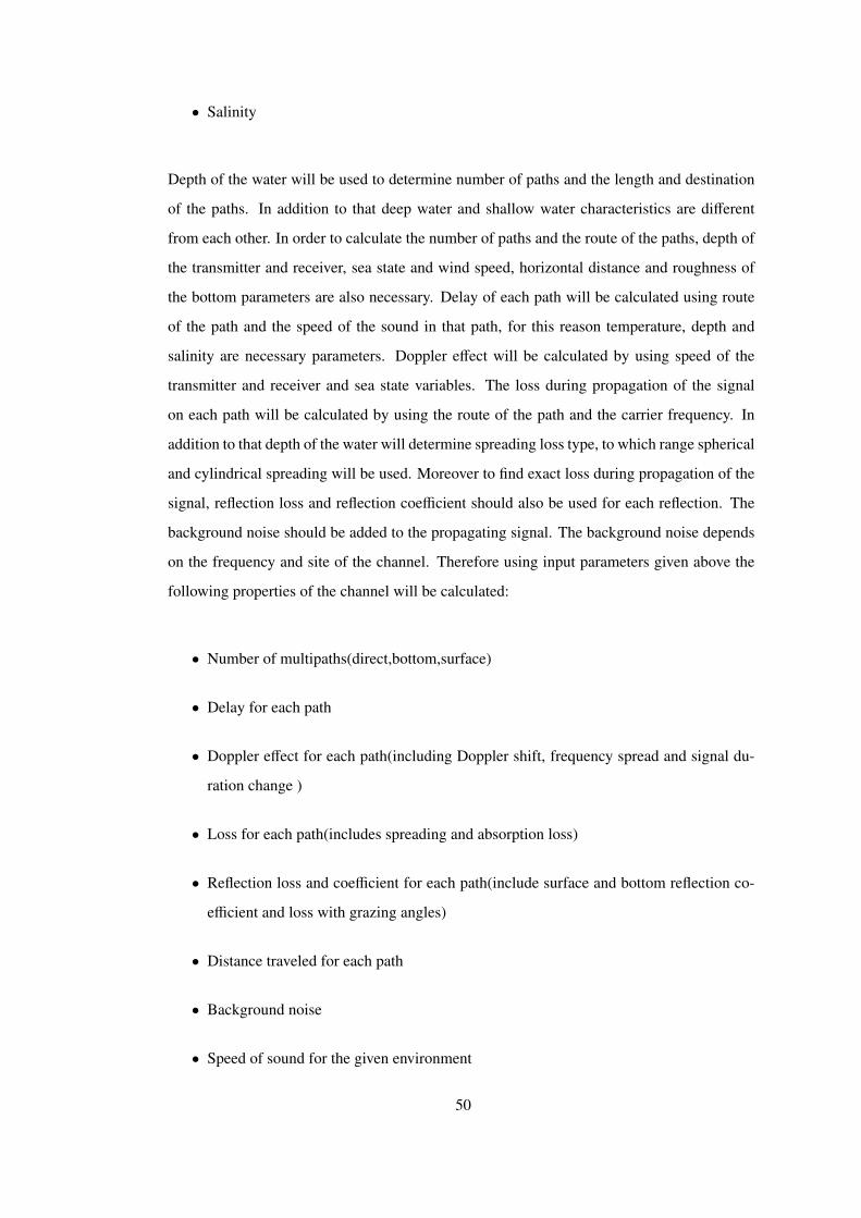
• Salinity
Depth of the water will be used to determine number of paths and the length and destination
of the paths. In addition to that deep water and shallow water characteristics are different
from each other. In order to calculate the number of paths and the route of the paths, depth of
the transmitter and receiver, sea state and wind speed, horizontal distance and roughness of
the bottom parameters are also necessary. Delay of each path will be calculated using route
of the path and the speed of the sound in that path, for this reason temperature, depth and
salinity are necessary parameters. Doppler effect will be calculated by using speed of the
transmitter and receiver and sea state variables. The loss during propagation of the signal
on each path will be calculated by using the route of the path and the carrier frequency. In
addition to that depth of the water will determine spreading loss type, to which range spherical
and cylindrical spreading will be used. Moreover to find exact loss during propagation of the
signal, reflection loss and reflection coefficient should also be used for each reflection. The
background noise should be added to the propagating signal. The background noise depends
on the frequency and site of the channel. Therefore using input parameters given above the
following properties of the channel will be calculated:
• Number of multipaths(direct,bottom,surface)
• Delay for each path
• Doppler effect for each path(including Doppler shift, frequency spread and signal du-
ration change )
• Loss for each path(includes spreading and absorption loss)
• Reflection loss and coefficient for each path(include surface and bottom reflection co-
efficient and loss with grazing angles)
• Distance traveled for each path
• Background noise
• Speed of sound for the given environment
50
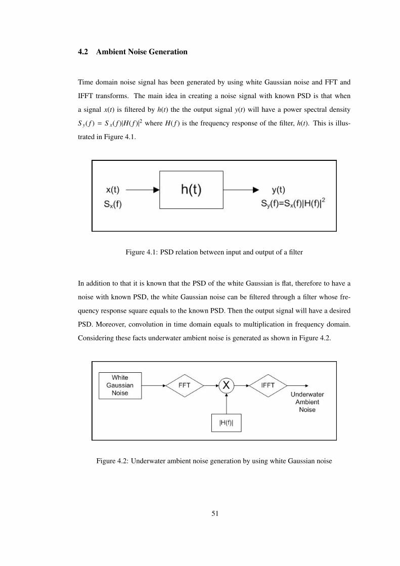
4.2 Ambient Noise Generation
Time domain noise signal has been generated by using white Gaussian noise and FFT and
IFFT transforms. The main idea in creating a noise signal with known PSD is that when
a signal x(t) is filtered by h(t) the the output signal y(t) will have a power spectral density
S y( f ) = S x( f )|H( f )|2 where H( f ) is the frequency response of the filter, h(t). This is illus-
trated in Figure 4.1.
Figure 4.1: PSD relation between input and output of a filter
In addition to that it is known that the PSD of the white Gaussian is flat, therefore to have a
noise with known PSD, the white Gaussian noise can be filtered through a filter whose fre-
quency response square equals to the known PSD. Then the output signal will have a desired
PSD. Moreover, convolution in time domain equals to multiplication in frequency domain.
Considering these facts underwater ambient noise is generated as shown in Figure 4.2.
Figure 4.2: Underwater ambient noise generation by using white Gaussian noise
51
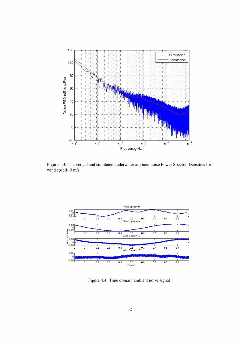
Figure 4.3: Theoretical and simulated underwater ambient noise Power Spectral Densities forwind speed=0 m/s
Figure 4.4: Time domain ambient noise signal
52
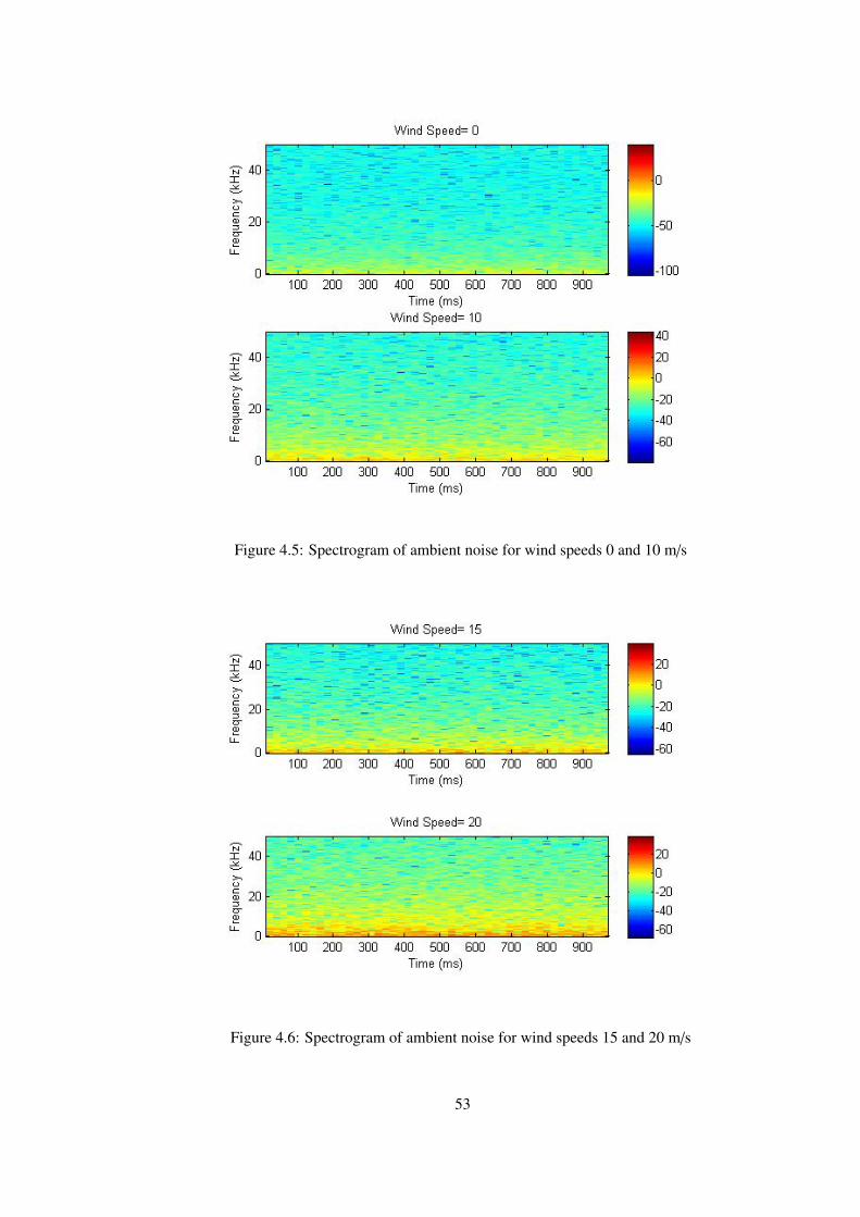
Figure 4.5: Spectrogram of ambient noise for wind speeds 0 and 10 m/s
Figure 4.6: Spectrogram of ambient noise for wind speeds 15 and 20 m/s
53
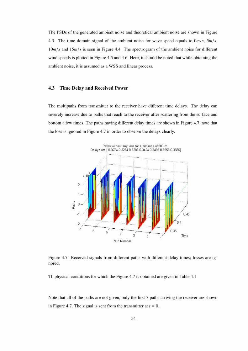
The PSDs of the generated ambient noise and theoretical ambient noise are shown in Figure
4.3. The time domain signal of the ambient noise for wave speed equals to 0m/s, 5m/s,
10m/s and 15m/s is seen in Figure 4.4. The spectrogram of the ambient noise for different
wind speeds is plotted in Figure 4.5 and 4.6. Here, it should be noted that while obtaining the
ambient noise, it is assumed as a WSS and linear process.
4.3 Time Delay and Received Power
The multipaths from transmitter to the receiver have different time delays. The delay can
severely increase due to paths that reach to the receiver after scattering from the surface and
bottom a few times. The paths having different delay times are shown in Figure 4.7, note that
the loss is ignored in Figure 4.7 in order to observe the delays clearly.
Figure 4.7: Received signals from different paths with different delay times; losses are ig-nored.
Th physical conditions for which the Figure 4.7 is obtained are given in Table 4.1
Note that all of the paths are not given, only the first 7 paths arriving the receiver are shown
in Figure 4.7. The signal is sent from the transmitter at t = 0.
54
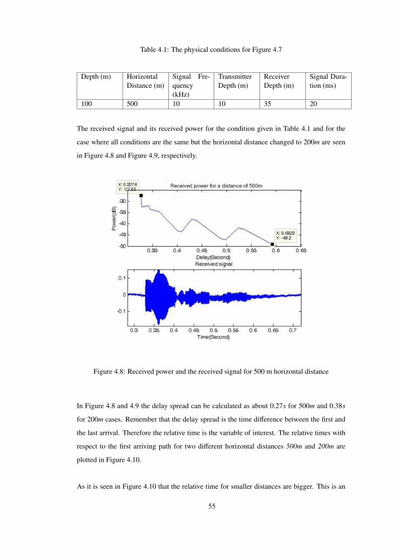
Table 4.1: The physical conditions for Figure 4.7
Depth (m) HorizontalDistance (m)
Signal Fre-quency(kHz)
TransmitterDepth (m)
ReceiverDepth (m)
Signal Dura-tion (ms)
100 500 10 10 35 20
The received signal and its received power for the condition given in Table 4.1 and for the
case where all conditions are the same but the horizontal distance changed to 200m are seen
in Figure 4.8 and Figure 4.9, respectively.
Figure 4.8: Received power and the received signal for 500 m horizontal distance
In Figure 4.8 and 4.9 the delay spread can be calculated as about 0.27s for 500m and 0.38s
for 200m cases. Remember that the delay spread is the time difference between the first and
the last arrival. Therefore the relative time is the variable of interest. The relative times with
respect to the first arriving path for two different horizontal distances 500m and 200m are
plotted in Figure 4.10.
As it is seen in Figure 4.10 that the relative time for smaller distances are bigger. This is an
55
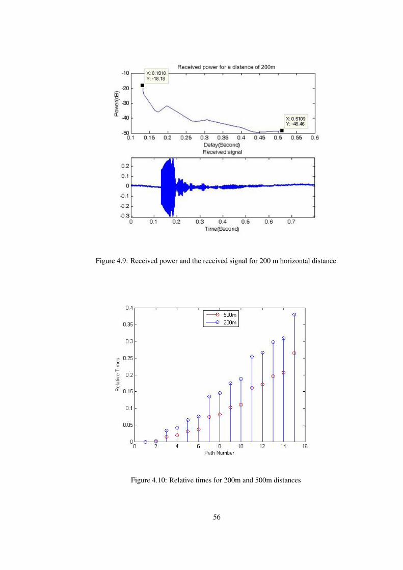
Figure 4.9: Received power and the received signal for 200 m horizontal distance
Figure 4.10: Relative times for 200m and 500m distances
56
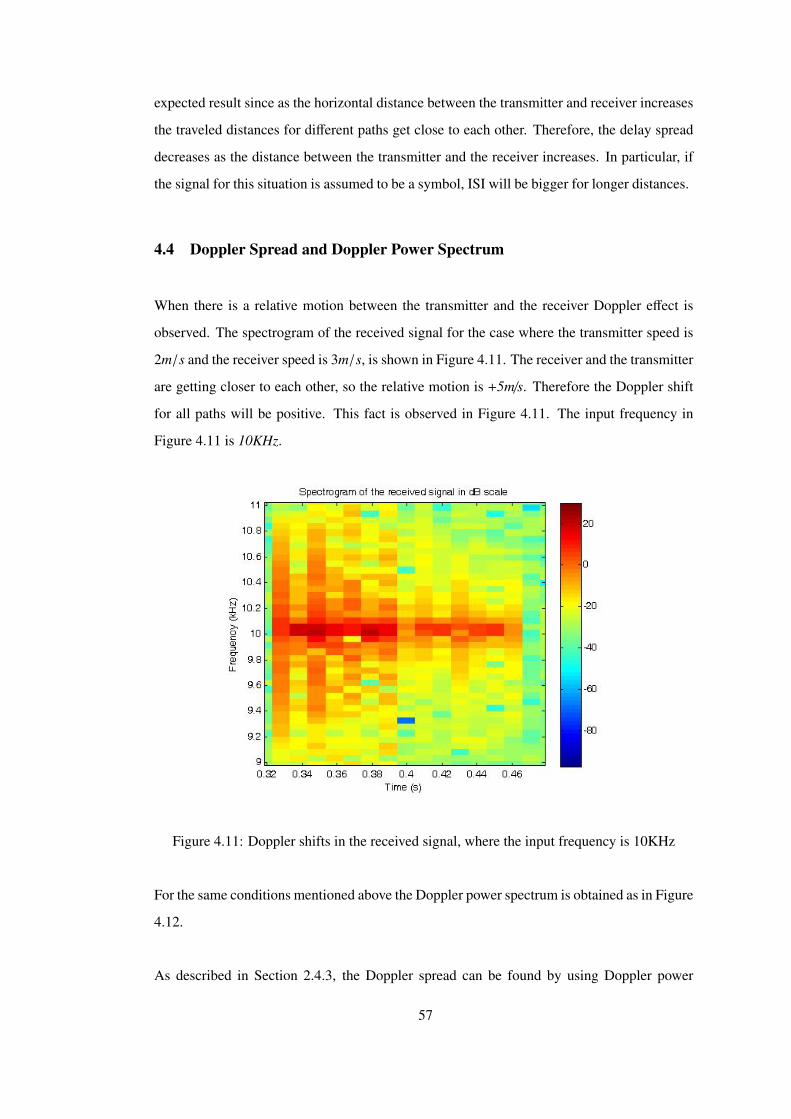
expected result since as the horizontal distance between the transmitter and receiver increases
the traveled distances for different paths get close to each other. Therefore, the delay spread
decreases as the distance between the transmitter and the receiver increases. In particular, if
the signal for this situation is assumed to be a symbol, ISI will be bigger for longer distances.
4.4 Doppler Spread and Doppler Power Spectrum
When there is a relative motion between the transmitter and the receiver Doppler effect is
observed. The spectrogram of the received signal for the case where the transmitter speed is
2m/s and the receiver speed is 3m/s, is shown in Figure 4.11. The receiver and the transmitter
are getting closer to each other, so the relative motion is +5m/s. Therefore the Doppler shift
for all paths will be positive. This fact is observed in Figure 4.11. The input frequency in
Figure 4.11 is 10KHz.
Figure 4.11: Doppler shifts in the received signal, where the input frequency is 10KHz
For the same conditions mentioned above the Doppler power spectrum is obtained as in Figure
4.12.
As described in Section 2.4.3, the Doppler spread can be found by using Doppler power
57
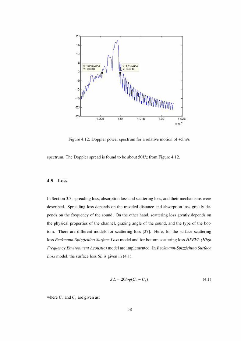
Figure 4.12: Doppler power spectrum for a relative motion of +5m/s
spectrum. The Doppler spread is found to be about 50Hz from Figure 4.12.
4.5 Loss
In Section 3.3, spreading loss, absorption loss and scattering loss, and their mechanisms were
described. Spreading loss depends on the traveled distance and absorption loss greatly de-
pends on the frequency of the sound. On the other hand, scattering loss greatly depends on
the physical properties of the channel, grazing angle of the sound, and the type of the bot-
tom. There are different models for scattering loss [27]. Here, for the surface scattering
loss Beckmann-Spizzichino Surface Loss model and for bottom scattering loss HFEVA (High
Frequency Environment Acoustic) model are implemented. In Beckmann-Spizzichino Surface
Loss model, the surface loss SL is given in (4.1).
S L = 20log(Cv −Cs) (4.1)
where Cv and Cs are given as:
58
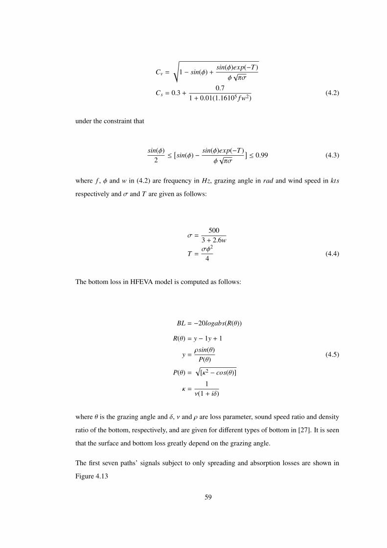
Cv =
√1 − sin(φ) +
sin(φ)exp(−T )φ√πσ
Cs = 0.3 +0.7
1 + 0.01(1.16105 f w2)(4.2)
under the constraint that
sin(φ)2≤
[sin(φ) −
sin(φ)exp(−T )φ√πσ
]≤ 0.99 (4.3)
where f , φ and w in (4.2) are frequency in Hz, grazing angle in rad and wind speed in kts
respectively and σ and T are given as follows:
σ =500
3 + 2.6w
T =σφ2
4(4.4)
The bottom loss in HFEVA model is computed as follows:
BL = −20logabs(R(θ))
R(θ) = y − 1y + 1
y =ρsin(θ)
P(θ)(4.5)
P(θ) =√
[κ2 − cos(θ)]
κ =1
ν(1 + iδ)
where θ is the grazing angle and δ, ν and ρ are loss parameter, sound speed ratio and density
ratio of the bottom, respectively, and are given for different types of bottom in [27]. It is seen
that the surface and bottom loss greatly depend on the grazing angle.
The first seven paths’ signals subject to only spreading and absorption losses are shown in
Figure 4.13
59
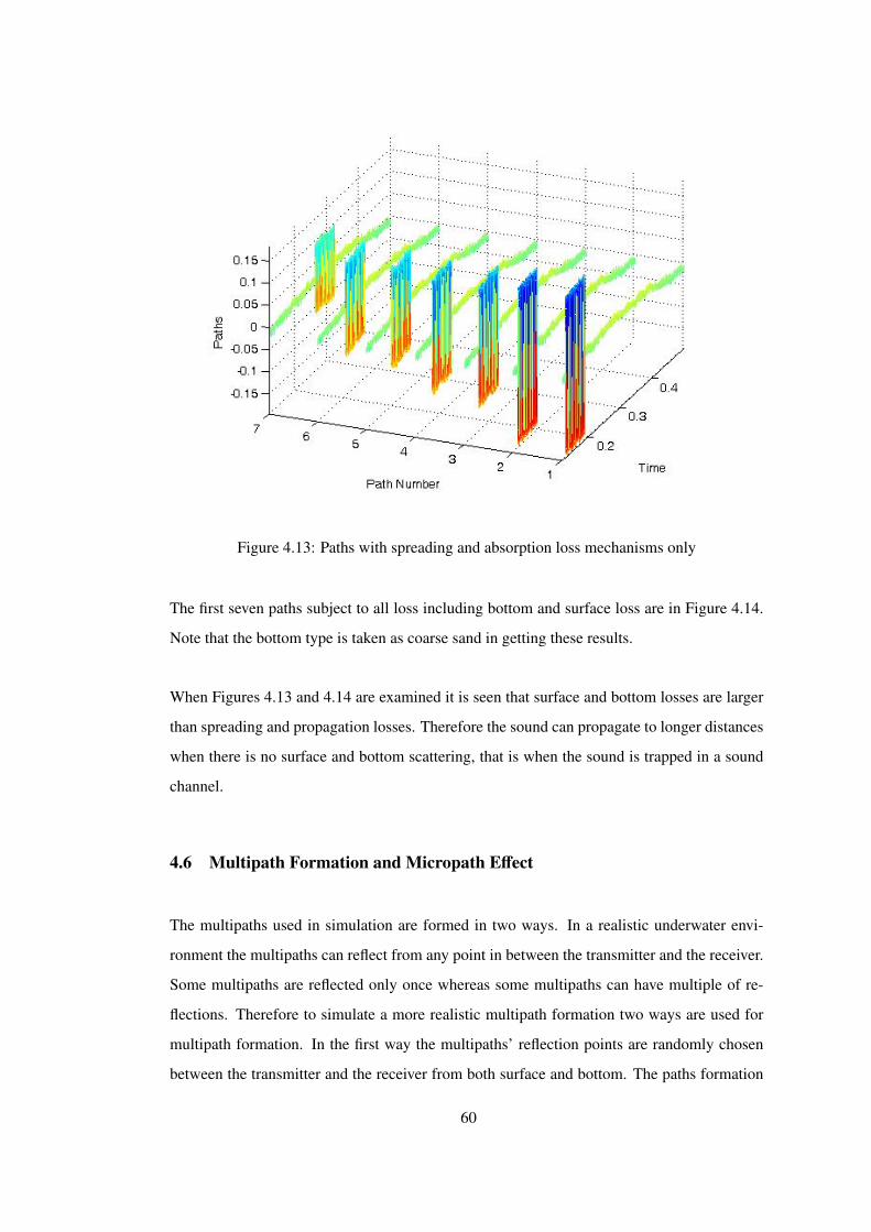
Figure 4.13: Paths with spreading and absorption loss mechanisms only
The first seven paths subject to all loss including bottom and surface loss are in Figure 4.14.
Note that the bottom type is taken as coarse sand in getting these results.
When Figures 4.13 and 4.14 are examined it is seen that surface and bottom losses are larger
than spreading and propagation losses. Therefore the sound can propagate to longer distances
when there is no surface and bottom scattering, that is when the sound is trapped in a sound
channel.
4.6 Multipath Formation and Micropath Effect
The multipaths used in simulation are formed in two ways. In a realistic underwater envi-
ronment the multipaths can reflect from any point in between the transmitter and the receiver.
Some multipaths are reflected only once whereas some multipaths can have multiple of re-
flections. Therefore to simulate a more realistic multipath formation two ways are used for
multipath formation. In the first way the multipaths’ reflection points are randomly chosen
between the transmitter and the receiver from both surface and bottom. The paths formation
60
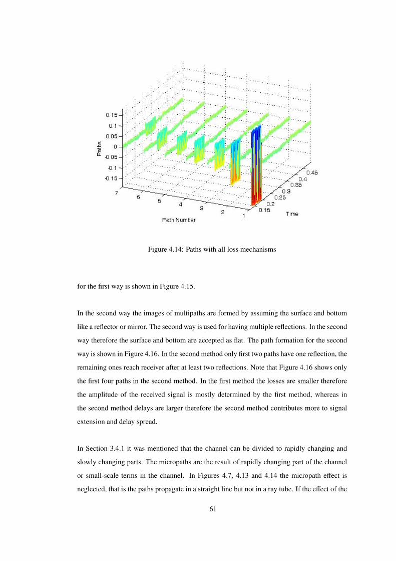
Figure 4.14: Paths with all loss mechanisms
for the first way is shown in Figure 4.15.
In the second way the images of multipaths are formed by assuming the surface and bottom
like a reflector or mirror. The second way is used for having multiple reflections. In the second
way therefore the surface and bottom are accepted as flat. The path formation for the second
way is shown in Figure 4.16. In the second method only first two paths have one reflection, the
remaining ones reach receiver after at least two reflections. Note that Figure 4.16 shows only
the first four paths in the second method. In the first method the losses are smaller therefore
the amplitude of the received signal is mostly determined by the first method, whereas in
the second method delays are larger therefore the second method contributes more to signal
extension and delay spread.
In Section 3.4.1 it was mentioned that the channel can be divided to rapidly changing and
slowly changing parts. The micropaths are the result of rapidly changing part of the channel
or small-scale terms in the channel. In Figures 4.7, 4.13 and 4.14 the micropath effect is
neglected, that is the paths propagate in a straight line but not in a ray tube. If the effect of the
61
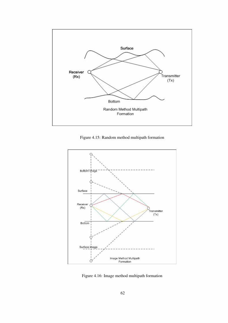
Figure 4.15: Random method multipath formation
Figure 4.16: Image method multipath formation
62
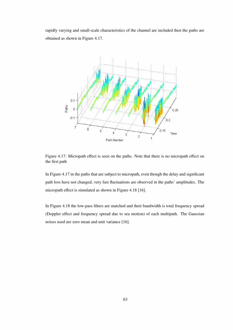
rapidly varying and small-scale characteristics of the channel are included then the paths are
obtained as shown in Figure 4.17.
Figure 4.17: Micropath effect is seen on the paths. Note that there is no micropath effect onthe first path
In Figure 4.17 in the paths that are subject to micropath, even though the delay and significant
path loss have not changed, very fast fluctuations are observed in the paths’ amplitudes. The
micropath effect is simulated as shown in Figure 4.18 [16].
In Figure 4.18 the low-pass filters are matched and their bandwidth is total frequency spread
(Doppler effect and frequency spread due to sea motion) of each multipath. The Gaussian
noises used are zero mean and unit variance [16].
63
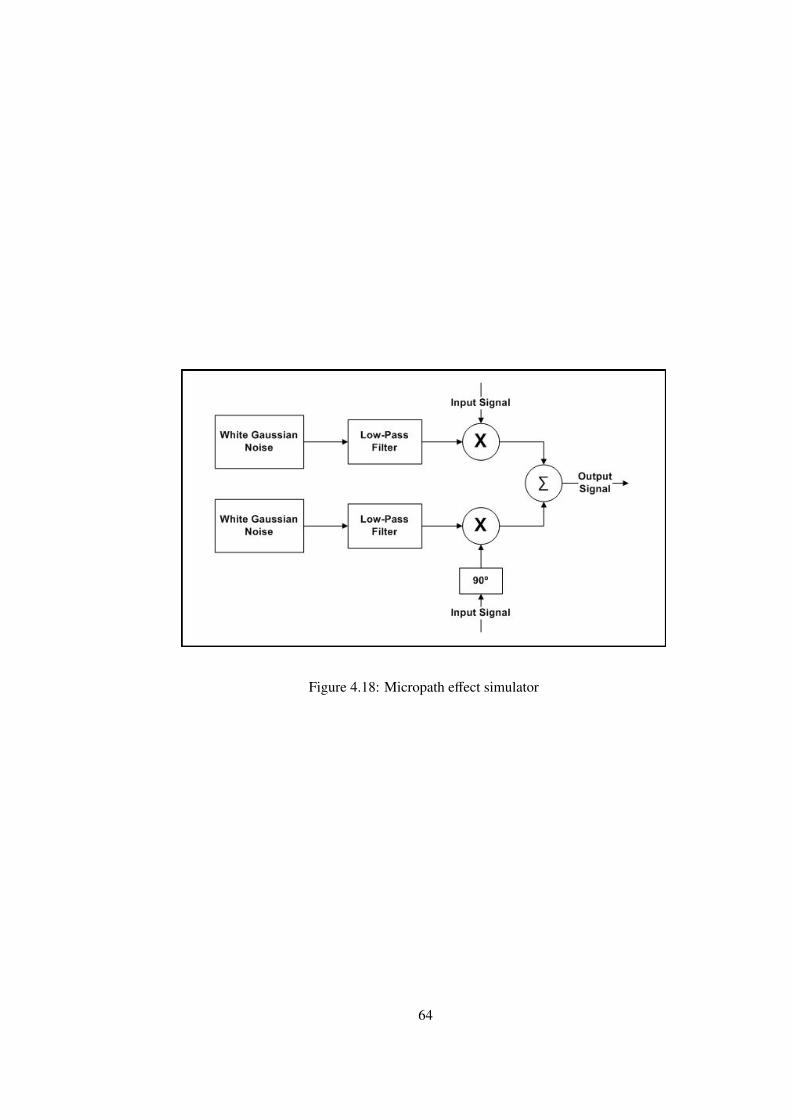
Figure 4.18: Micropath effect simulator
64
CHAPTER 5
MODEL FITTING TO EXPERIMENTAL DATA
This chapter is removed.
5.1 Introduction
5.2 Optimization of Channel Parameters
5.2.1 Optimizing the Sound Speed
5.2.2 Optimizing the Number of Paths
65
CHAPTER 6
CONCLUSION
In this thesis an underwater channel simulation and parameter optimization is conducted.
Firstly a general literature review has been done about multipath fading channels, underwater
physical properties and existing underwater channel models. The mathematical models of
these concepts are determined and used for simulation purpose. Secondly a channel model
is implemented in which nearly all physical properties of underwater environment including
randomness, Doppler effect and inherent inhomogeneities of the underwater environment are
modeled. Finally the model parameters are optimized by the help of experimental data for
specific scenarios.
The missing knowledge of the transmitter side and phase forced us to conduct the channel
identification in frequency domain, however, to obtain a good result the identification pro-
cedure should be conducted in time domain. The magnitude operation also decreases the
performance of channel identification, since instead of matching complex and real parts the
magnitude is matched, and the magnitude can be the same for different signals having dif-
ferent complex and real parts. In addition to that, nonlinear part of underwater channel are
neglected. The channel is assumed as a WSS and linear channel.
6.1 Results
Underwater channel is a dynamic and continuously changing environment. There is no such
a channel impulse response that can be used for every underwater channel but rather there are
lots of versions of underwater channel impulse response specific to each local zone and day
time. This is because a little fluctuation in temperature, wind speed, noise and other factors
66
that effect underwater environment results in a completely different channel impulse response.
The attenuation in underwater environment does not depend only on distance but also on fre-
quency, temperature, salinity and depth as well. The frequency increase results in attenuation
increase whereas the temperature and salinity increase results in attenuation decrease. On the
other hand, depth increase results in attenuation decrease. Moreover since there is no reflec-
tion loss in deep water the propagation distance of deep water is greater than that of shallow
water. The attenuation increase due to frequency increase obligates to use low frequencies in
underwater systems. Moreover since it is necessary to work at low frequencies and bandwidth
is comparable to carrier frequency underwater channels are accepted to be wideband.
Surface and bottom reflections with refractions due to inhomogeneity of sound speed cause
propagation of the transmitted signal to the receiver over multipaths. The number of multi-
paths are completely random and are actually very large but the ones under noise level are
ignored and the ones that have very close delay can be accepted as one multipath. If there
was not multipath effect in underwater systems the stochastic property of the channel was
going to decrease and moreover the complexity of the channel was going to decrease. In this
situation the only path that the transmitted signal propagates was going to be direct path and
that path was going to be characterized by just a nearly determined loss and delay. Therefore,
the complexity and difficulty of the channel is mostly due to multipath effect.
The simulated channel characterization functions seem to be not consistent very well with
that of real channel for the same physical conditions. In addition that the decision of number
of paths parameter was difficult. Therefore an optimization of number of paths was neces-
sary. Moreover, it was found that for the given real channel the temperature and salinity are
not known therefore the sound speed that will be determined theoretically would not agree
exactly to the real one since the temperature and salinity parameters used for theoretical cal-
culation was going to be average values. Hence an optimization procedure is implemented
for both of these variables. It was found that after optimization procedure the characterization
functions were more consistent for simulated and real channel. For number of paths optimiza-
tion it cannot be said that the obtained number is exactly giving the number of paths that the
transmitted signal propagates, however it can be said that the simulated channel best fits to
real channel under these number of paths.
67
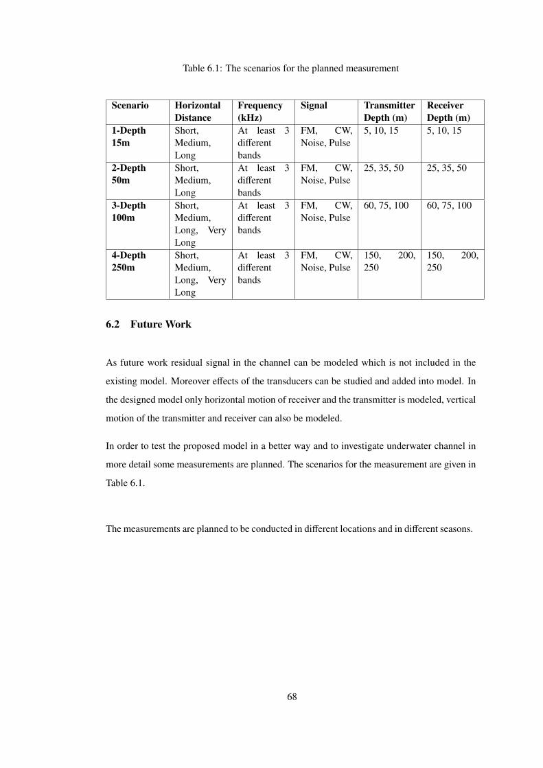
Table 6.1: The scenarios for the planned measurement
Scenario HorizontalDistance
Frequency(kHz)
Signal TransmitterDepth (m)
ReceiverDepth (m)
1-Depth15m
Short,Medium,Long
At least 3differentbands
FM, CW,Noise, Pulse
5, 10, 15 5, 10, 15
2-Depth50m
Short,Medium,Long
At least 3differentbands
FM, CW,Noise, Pulse
25, 35, 50 25, 35, 50
3-Depth100m
Short,Medium,Long, VeryLong
At least 3differentbands
FM, CW,Noise, Pulse
60, 75, 100 60, 75, 100
4-Depth250m
Short,Medium,Long, VeryLong
At least 3differentbands
FM, CW,Noise, Pulse
150, 200,250
150, 200,250
6.2 Future Work
As future work residual signal in the channel can be modeled which is not included in the
existing model. Moreover effects of the transducers can be studied and added into model. In
the designed model only horizontal motion of receiver and the transmitter is modeled, vertical
motion of the transmitter and receiver can also be modeled.
In order to test the proposed model in a better way and to investigate underwater channel in
more detail some measurements are planned. The scenarios for the measurement are given in
Table 6.1.
The measurements are planned to be conducted in different locations and in different seasons.
68
REFERENCES
[1] A. Goldsmith. Wireless Communications. Cambridge University Press, Cambridge,2005.
[2] H. V. Poor and G. W. Wornell. Wireless Communication Signal Processing Perspectives,chapter 8: Underwater Acoustic Communications. Prentice Hall, New Jersey, 1998.
[3] M. Stanjovic. Underwater Acoustic Communications: Design Considerations on thePhysical Layer. Wireless on Demand Network Systems and Services. WONS 2008. FifthAnnual Conference, 2008.
[4] J. Preisig and M. Stanjovic. Underwater Acoustic Communication Channels: Propaga-tion Models and Statistical Characterization. IEEE Communication Magazine, January2009.
[5] Z. Jiang. Underwater Acoustic Networks: Issues and Solutions . International Journalof Intelligent Control and Systems, 13:152–161, Sep 2008.
[6] M. Stanjovic. Recent Advances in High-speed Underwater Acoustic Communications .IEEE Journal Of Oceanic Engineering, 21:125–136, april 1996.
[7] A. B. Baggeroer, J. C. Preisig, and T. H. Eggen. Communication Over Doppler SpreadChannels Part I: Channel and Receiver Presentation. IEEE Journal Of Oceanic Engi-neering, 25:62–71, January 2000.
[8] M. Chitre. A High-Frequency Warm Shallow Water Acoustic Communications ChannelModel and Measurements. Acoustical Society of America, November 2007.
[9] R. Galvin and R.F.W. Coates. A Stochastic Underwater Acoustic Channel Model. IEEEOCEANS, 1:203–210, Sep 1996.
[10] W. B. Yang and T. C. Yang. Characterization and Modeling of Underwater AcousticCommunications Channels for Frequency-Shift-Keying Signals. IEEE OCEANS, pages1–6, September 2006.
[11] G. Bertolotto, P. V. Walree, and T. Jenserud. Initial Design of an Acoustic Communica-tion Channel Simulator. RTP 110.060 UUV Covert Acoustic Communications Project,2007.
[12] H. P. Bucker and M. B. Porter. Gaussian Beam Tracing for Computing Ocean AcousticFields. J. Acoust. Soc. Am., 82:1349–1359, 1987.
[13] A. Sehgal. Analysis and Simulation of the Deep Sea Acoustic Channel for Sensor Net-works. Master’s thesis, Jacobs University, Bremen, Germany, 2009.
[14] A. Bouzoualegh, Th. Val, E. Campo, and F. Peyrard. Modelling and Simulation ofUnderwater Acoustic Communication Based on Stateflow and Simulink Models. SETIT,March 2005.
69
[15] M. A. M. Gutierrez, P. L. P. Sanchez, and J. V. V. Neto. An Eigenpath Underwa-ter Acoustic Communication Channel Simulation. OCEANS, 2005. Proceedings ofMTS/IEEE, 1:355–362, 2005.
[16] A. Zielinski and X. Geng. An Eigenpath Underwater Acoustic Communication ChannelModel. OCEANS ’95. MTS/IEEE. Challenges of Our Changing Global Environment.Conference Proceedings., 2:1189 – 1196, January 1995.
[17] R. Pattarkine. High Rate OFDM Acoustic Link for Underwater Communication. PVGsCollege of engineering and Technology, November.
[18] B. Sklar. Rayleigh Fading Channels in Mobile Digital Communication Systems. IEEECommun. Mag, 35(7):90–100, July 1997.
[19] L. M. Brekhovskikh and Y. P. Lysonov. Fundementals of Ocean Acoustics. Springer-Verlag, Berlin, 1991.
[20] Y. L. Sun and Z.Han. Cooperative Transmission for Underwater Acoustic Communica-tions. IEEE International Conferences on Communication, May 2008.
[21] E. M. Sozer, J.G. Proakis, and M. Stojanovic. Underwater Acoustic Networks. IEEEJournal of Oceanic Engineering, 25(1), January 2000.
[22] M. Stojanovic. Underwater Acoustic Communication. Quart. Progr. Rept., Entry Forthe Wiley Encyclopedia of Electrical and Electronics Engineering, 1999.
[23] P. King, R.Venkatesan, and C. Li. Modeling a Shallow Water Acoustic communicationChannel Using Environmental Data for Seafloor Sensor Networks. Wireless Commini-cations and Mobile Computing, OCT 2009.
[24] A. C. Singer, J. K. Nelson, and S. S. Kozat. Signal Processing For Underwater AcousticCommunications. IEEE Communication Magazine, 47:90 – 96, January 2009.
[25] Z. Guoqing and S. Taebo. Simulation Analysis of High Speed Underwater AcousticCommunication Based on a Statistical Channel Model. Image and Signal Processing,2008. CISP ’08., 5:512–517, May 2008.
[26] A. Essebbar, G. Loubet, and F. Vial. Underwater Acoustic Channel Simulations forCommunication. in OCEANS ’94 Proc, 3:495–500, Sep 1994.
[27] R.P. Hodges. Underwater Acoustics: Analysis, Design and Performance of Sonar. Wi-ley, West Sussex, 2010.
70