AN UNDULATOR BASED ON BEAM DRIVEN WAKEFIELDS IN A DIELECTRIC TUBE

Josh Cutler

UCLA Department of Physics & Astronomy, Los Angeles, CA 90095

March 2012

1 INTRODUCTION

Light sources are devices which produce brilliant X-rays used in researching topics from medicine to geology. Free electron lasers (FELs) are now providing the latest generation of light sources. The free electron laser is composed of an electron source, an accelerator, and an undulator. Our focus is on the undulator. The oscillation of an electron bunch through the undulator generates photons. The wavelength of released photons can be decreased with a shortened undulator period. The magnetic undulators, which are the most common, are difficult to produce with periods shorter than the order of cm.

We are focusing on a new approach in producing the undulator field. Instead of using the typical magnetic undulator, we are using a dielectric tube to simulate the same wakefield pattern seen in traveling wave undulators. With the proper tube structure, a single mode can be generated from an electron bunch and create wakefields in the THz range (infrared) using coherent Cherenkov radiation as shown below in Figure 1. The lowest transverse electric mode is preferred because the electron beam would follow a helical path due to the wakefield. Such a beam-driven structure could be used to produce an undulator-like field with periods less than 1 mm and frequencies on the order of terahertz. [1]

Figure 1: The nature of coherence. We want the wakefields left by the first electron bunch to make the next bunch coherent.

2 THEORY

2.1 FEL AND UNDULATOR DESIGN

In order to generate infrared wakefield radiation in the FEL, we needed to alter the undulator period and electron energies for the following formula to work:

λ r=λu

2 γ 2 (1+au

2

2 ) (1)

where λu is the undulator period, γ is the Lorentz factor, and au is the dimensionless normalized field strength. To find these variables, we started with previously determined values that were useful to us.

We chose λr to be 10-10 m because of its previous FEL use in the LCLS x-rays. This wavelength of x-rays is also the approximate radius of an atom. [2]

Because of its success in previous dielectric wakefield accelerator experiments on the order of 1 THz, we chose λu =300 μm.

We chose au based on:

au=e λu Bu

2π me c≈ 0.94 λu Bu (2)

Since we are only approximating on orders at this stage and would look at ranges later, we put au on the order of 1. When we substitute these parameters back into equation (1), γ is approximately 1500, which signifies that the beam has energy of 0.75 GeV.

Table 1: FEL parameters

Radiation wavelength, Å 1.0Undulator period, μm 300Undulator parameter 1Beam energy, GeV 0.75

To find the peak electric field at the inner surface of the dielectric, we can substitute Bu= Er , surf

c,

and we will get Er ,surf ≈1010V /m=10 GV /m. The wakefield driven dielectric breakdown is about13.8 GV/m, so this result is within breakdown level. [3]

Using the above electric field, we can find approximations for inner radius a, bunch length σ z, and electron amount N b as shown below:

Er ,surf =

4 Nb re me c2

ae (√ 8 πεr−1

εr σ z+a)

(3)

where re is the classical electron radius, me is the mass of the electron, e is the charge of the electron, and εr is the dielectric constant. The dielectric is made of fused silica due to its availability, so εr=3.8. [4]

The data combination of a=200 μm, σ z=100 μm, and N b=109 electrons worked best for a radial electric field on the order of 107 V/m on the inner radius, which is far below Er ,surf above. Our next goal was to modify these values to get a TE01 mode frequency of 1 THz in a tube waveguide.

2.2 RESONANT FREQUENCIES OF DIELECTRIC TUBE

The TE01 frequencies are given by:

f 0 1=1

2 πβcκ0 1

√εr β2−1 (4)

where κ is the wavenumber determined by the energy of the electron and γ=1

√1−β2 . The tube

radii are given by inner radius a and outer radius b. [5]

We want to generate TE01 frequencies close to 1 THz with an appropriate tube waveguide based on the energy of the electron bunch and radii of the tube as shown above in Equation (4). This would generate wakefields that can accelerate the next electron bunch if they are coherent. We desire a transverse electric mode from this bunch to amplify the photon emissions through self-amplified stimulated emission. Because of this process, SASE could negate the need for an external power source in an undulator.

The parameters and process leading to Equation (4) were evaluated on a Mathematica file based in Alan Cook’s longitudinal wakefield analysis.

2.3 WAKEFIELD EXCITATION OF TUBE (OOPIC)

An OOPIC simulation was used to display the wakefield excitation of the tube. The OOPIC simulations need to be consistent with the generated electric field in Mathematica to prove that these parameters will generate one transverse mode in a simulation. The required frequency of 1 THz must also be generated to verify that the intended design could work with an actual dielectric tube modeled after the undulator.

3 NUMERICAL RESULTS

In Mathematica and OOPIC, we tested different undulator radii and bunch lengths to see if we can yield a wakefield with a 1 THz frequency.

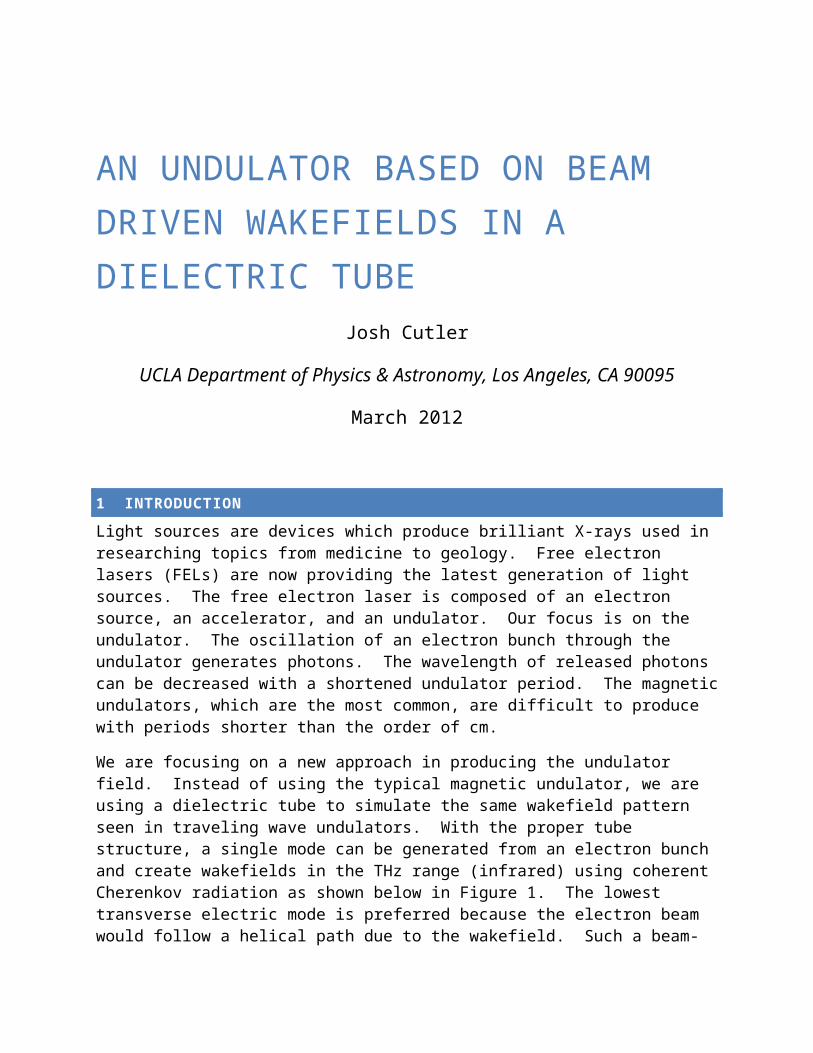
When we tested each value of inner radius a for certain ratios of b:a (εr=3.8, γ=1500), we got these THz values for f01:

Table 2: Radii ratios and wakefield frequencies

a b:a=1.5:1 b:a=1.75:1 b:a=2:1 b:a=2.25:1 b:a=2.5:150 2.9 2.07 1.61 1.33 1.1375 1.93 1.38 1.08 0.89 0.76100 1.45 1.03 0.81 0.67 0.57125 1.16 0.83 0.65 0.53 0.45150 0.97 0.69 0.54 0.44 0.38

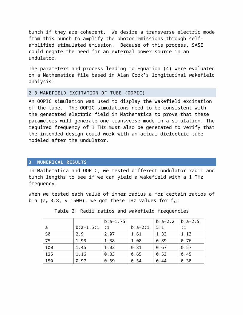
Figure 2: Radii Ratio Chart

Next, we tested the values of σz and Nb for the radii ratios that had frequencies within 0.1 THz of 1 THz to see which ones yielded a sinusoidal wakefield with a sufficiently strong amplitude (Nb=109):

Table 3: Mathematica results

a (μm) b (μm) σz (μm) THz Frequency E amplitude (V/m)150 225 75 0.97 1.22x107

100 175 70 1.03 1x107

75 150 60 1.08 8.71x106

1.5 1.6 1.7 1.8 1.9 2 2.1 2.2 2.3 2.4 2.50

0.5

1

1.5

2

2.5

3

3.5Radii ratios

50 micron radius

75 micron radius

100 micron radius

125 micron radius

150 micron radius

Outer:Inner radius ratio

Wak

efiel

d fr

eque

ncy

(THz

)

0.0002 0.0000 0.0002 0.0004 0.0006 0.0008 0.0010

1 10 7

5 10 6

0

5 10 6

1 10 7

s m E z

Vm

Longitudinal Wakefield E z

Figure 3: Mathematica Longitudinal Wakefield for a=150 μm, b=225 μm

0.0002 0.0000 0.0002 0.0004 0.0006 0.0008 0.0010 1 10 7

5 10 6

0

5 10 6

1 10 7

s m

E zVm

Longitudinal W akefield E z

Figure 4: Mathematica Longitudinal Wakefield for a=100 μm, b=175 μm

0.0002 0.0000 0.0002 0.0004 0.0006 0.0008 0.0010

5 10 6

0

5 10 6

s m

E zVm

Longitudinal Wakefield E z

Figure 5: Mathematica Longitudinal Wakefield for a=75 μm, b=150 μm

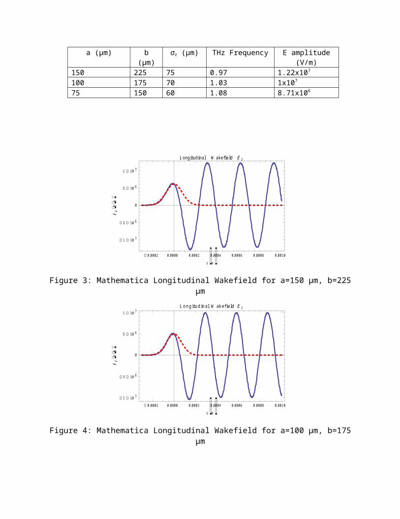
All of these wakefields had a magnitude near 107 V/m: the desired straw-man wakefield amplitude.

In OOPIC, we tested the parameters that worked to see which longitudinal wakefield graph would resemble the Mathematica plot and also give a 1 THz frequency. An axial field was calculated at r=0 and the radial field was calculated at r=a. Here are the results:

Table 4: OOPIC Simulation results

a (μm) b (μm) σz (μm) Beam radius (μm)

THz Frequency

Longitudinal E amplitude

(V/m)

Radial E amplitude

(V/m)150 225 75 91 0.53 7.13x107 4.02x107

100 175 70 91 0.59 1.08x108 6.66 x107

75 150 60 61 0.57 1.8x108 8.48 x107

0.000 0.002 0.004 0.006 0.008

6 10 7

4 10 7

2 10 7

0

2 10 7

4 10 7

6 10 7

z m

E zVm

Longitudinal W akefield E z

Figure 6: OOPIC Longitudinal Wakefield for a=150 μm, b=225 μm

0.000 0.001 0.002 0.003 0.004 0.005 0.006

1 10 8

5 10 7

0

5 10 7

1 10 8

z m

E zVm

Longitudinal W akefield E z

Figure 7: OOPIC Longitudinal Wakefield for a=100 μm, b=175 μm

0.000 0.001 0.002 0.003 0.004 0.005

1.5 10 8

1.0 10 8

5.0 10 7

0

5.0 10 7

1.0 10 8

1.5 10 8

z m E z

Vm

Longitudinal Wakefield E z

Figure 8: OOPIC Longitudinal Wakefield for a=75 μm, b=150 μm

0.000 0.002 0.004 0.006 0.008

8 10 7

6 10 7

4 10 7

2 10 7

0

2 10 7

4 10 7

z m

E rVm

Radial W akefield E r

Figure 9: OOPIC Radial Wakefield for a=150 μm, b=225 μm

0.000 0.001 0.002 0.003 0.004 0.005 0.006

1.5 10 8

1.0 10 8

5.0 10 7

0

5.0 10 7

z m

E rVm

Radial Wakefield E r

Figure 10: OOPIC Radial Wakefield for a=100 μm, b=175 μm

0.000 0.001 0.002 0.003 0.004 0.005 1.5 10 8

1.0 10 8

5.0 10 7

0

5.0 10 7

z m E r

Vm

Radial Wakefield E r

Figure 11: OOPIC Radial Wakefield for a=75 μm, b=150 μm

4 DISCUSSION

As we can see from Figures 6-11, the problem with the OOPIC simulations is that we have had trouble creating a sinusoidal wakefield due to the interference of other modes. This could be why the wakefield measurements are so erratic and the frequency only came within half of its expected value.

When the straw-man design was tested on OOPIC, the resonant frequency did not come close to 1 THz. However, these figures were approximations to be modified for the simulations above. This tube is possible to engineer if we can build one on the order of hundreds of μm.

The best measurements of frequency and an almost sinusoidal wakefield come from inner radius 100 μm, outer radius 175 μm, and bunch length 70 μm. However, simulation results indicate that the tube structure is still flawed, perhaps due to the beam radius or number of electrons.

5 CONCLUSIONS

After reanalyzing Cook’s Mathematica file and his dissertation, we believe the reason that the frequencies haven’t come close to 1 THz is because we were generating a TM mode, and not a TE mode. The field at the boundary of the dielectric resembles the TM mode, despite changing the TE01 frequency in Mathematica.

In order to achieve a wakefield frequency of 1 THz, we plan to generate a dipole mode like HEM11 or TE11.

1 C. Pellegrini: “X-Band Microwave Undulators for Short Wavelength Free-Electron Lasers”2 LCLS Glossary: http://www-ssrl.slac.stanford.edu/lcls/glossary.html3 M.C. Thompson et al., Phys. Rev. Letter: “Breakdown Limits on Gigavolt-per-meter Electron-beam-driven wakefield in Dielectric Structures”4 A.M. Cook et al.: “Beam-driven dielectric wakefield accelerating structure as a THz radiation source”5 A.M. Cook: “Generation of Narrow-Band Terahertz Coherent Cherenkov Radiation in a Dielectric Wakefield Structure”