unified backwards facing and forwards facing simulation of

This item was submitted to Loughborough's Research Repository by the author. Items in Figshare are protected by copyright, with all rights reserved, unless otherwise indicated.

Unified backwards facing and forwards facing simulation of a hybrid electricUnified backwards facing and forwards facing simulation of a hybrid electricvehicle using MATLAB Simscapevehicle using MATLAB Simscape

PLEASE CITE THE PUBLISHED VERSION

http://dx.doi.org/doi:10.4271/2015-01-1215

PUBLISHER

© SAE International

VERSION

AM (Accepted Manuscript)

PUBLISHER STATEMENT

Copyright © 2015 SAE International. This paper is posted on this site with permission from SAE International.It may not be shared, downloaded, transmitted in any manner, or stored on any additional repositories orretrieval system without prior written permission from SAE.

LICENCE

All Rights Reserved

REPOSITORY RECORD

Dixon, George, Richard Stobart, and Thomas Steffen. 2015. “Unified Backwards Facing and Forwards FacingSimulation of a Hybrid Electric Vehicle Using MATLAB Simscape”. figshare. https://hdl.handle.net/2134/17461.

https://lboro.figshare.com/

http://dx.doi.org/doi:10.4271/2015-01-1215

of 12

2015-01-1215

Unified backwards facing and forwards facing simulation of a hybrid electric vehicle using MATLAB Simscape

G. Dixon, T. Steffen, R. Stobart Department of Aeronautical and Automotive Engineering, Loughborough University, UK

Abstract

This paper presents the implementation of a vehicle and powertrain model of the parallel hybrid electric vehicle which can be used for several purposes: as a model for estimating fuel consumption, as a model for estimating performance, and as a control model for the hybrid powertrain optimisation. The model is specified as a multi-domain physical model in MATLAB Simscape, which captures the key electrical, mechanical and thermal energy flows in the vehicles. By applying hand crafted boundary conditions, this model can be simulated either in the forwards or backwards direction, and it can easily be simplified as required to address specific control problems.

Modelling in the forwards direction, the driver inputs are specified, and the vehicle response is the model output. In the backwards direction, the vehicle velocity as a function of time is the specified input, and the engine torque, and fuel consumption are the model outputs.

The model represents a parallel hybrid vehicle, which is being developed in the TC48 project. The project goal is to produce a prototype of a plug-in parallel hybrid system which is integrated into existing front wheel drive powertrains with modest additional engineering, cost, volume, and mass requirements.

This paper explains the motivation for the project, and presents examples of the simulations which were used to guide the design. The vehicle simulation models used to evaluate the layout options are described and discussed. Sensitivity analyses are presented which informed the design decisions.

A novel use of the Simscape component of MATLAB/Simulink which allows the same model structure to be used for both forwards and backwards simulations is demonstrated. This method has the possibility for more general application, and a toolbox is being developed which assists the generation of mathematical models of this type.

Introduction

The TC48 project, [3], aims to demonstrate the possibility of packaging a parallel electric hybrid powertrain within the engine compartment of a front wheel drive passenger car.

The advantages of such a powertrain are;

1. Simplified integration into the manufacturing process when assembled alongside conventional vehicles,

2. Modest additional engineering, cost, mass, and volume requirements,

3. The ability to use an electric vehicle mode, allowing the vehicle to enter into city centre low emission zones,

4. Improved combination of performance, economy, and emissions when compared with a conventional vehicle.

The TC48 hybrid architecture and control strategy minimizes battery costs, whilst seamlessly blending Plug-in Hybrid Electric Vehicle (PHEV) Town mode capable of a 15 mile All Electric Range (AER) with Hybrid Electric Vehicle Country mode where higher speeds are demanded.

The parallel powertrain system allows the summation of IC engine torque and electric motor torque when operating in hybrid mode, with the distinction that the electric motor torque may be negative during charging. The vehicle may be used in electric only mode, with the vehicle’s clutch acting to disengage the IC engine from the drivetrain.

Owing to the constraints of battery packaging within the engine compartment, it is not envisaged for the vehicle to have a significant electric only range. The electric only operating mode is targeted at low speed, city centre motoring, while the IC engine and hybrid operating modes are targeted for higher speed operation.

The TC48 project provided an impetus to consider the simplification of vehicle modelling activity, and to consider the possibility of producing one dynamic model which can form the basis of both a forwards and backwards looking simulation. This has been identified as a desirable method in previous studies of conventional vehicles, [5], and this paper aims to update the work using newly available tools and to hybrid electric powertrains.

Vehicle Simulation

In order to inform the initial sizing of components and the evolution of an efficient layout, mathematical simulations of vehicle performance were required, [10], [11].

Initial Model

For speed, the initial forwards and backwards models were built using MATLAB / Simulink, [2], and the blocks in the QSS toolbox,

of 12

[12]. These initial models verified the feasibility of the project, and allowed initial sensitivity studies to be undertaken.

Among the findings from this initial simulation were;

1. Wheelspin in hybrid mode in the lower gears was likely under conditions of high driver demand

2. The efficiency of the gearbox is an important factor as both the power from the internal combustion engine and the electric motor is passed through it.

3. When operating in hybrid mode, owing to their smaller numeric value, typical overall gear ratios for the diesel engined cars in the range under consideration were more suitable than those from the equivalent petrol engine vehicles.

The power at the wheels and the road load power are plotted in figure 1.

Figure 1. Power at wheels, Electric Motor + IC Engine

The power at the wheels minus the road load power gives the power available to accelerate the vehicle. The vehicle’s acceleration may be estimated by dividing the available power by the product of the velocity and effective mass. The acceleration in each gear is plotted in figure 2. The crossing points of these curves indicate the gear change points for optimum acceleration.

Figure 2. Optimum Gear Change Points, Electric Motor + IC Engine

The initial model did not consider;

1. Gear changing delay time, 2. The electric motor was not modelled in detail, mean value data

were used, 3. No calculation was made of fuel consumption or electrical

energy use, 4. Friction was modelled using one coefficient, i.e., no distinction

was made between static and dynamic tyre/road friction 5. No account was made of different loading states of the vehicle 6. The transmission losses were modelled using a single loss

coefficient, i.e., no account was made of the effects of load and speed on efficiency.

Sensitivity Study

The initial model was used as a basis for sensitivity study. Working from the baseline data, one parameter at a time was varied. Each parameter was varied by -10%, -5%, +5%, and +10%. While there are some parameters which only took integer values, for example, the number of batteries, fictitious fractional variations can indicate trends. For each case, the maximum gradient where the vehicle would obtain sufficient grip to set off was estimated. Using the tractive effort required to allow the vehicle to move off, and the electric motor torque and gearbox efficiency, the overall reduction ratio for first gear was estimated.

Using the overall first gear ratio, and the overall top gear ratio which is a tuneable parameter, the intermediate gears were found using a progressive gear ratio layout, [13]. The tuneable parameter, φ2, was used to tune the degree of progression. Using progressive gear spacing, the gear step reduces in the higher gears. This is more suitable for passenger cars, giving closer ratios at speed.

( )( )1 215.02

1 −−−= z zz

TOTALrϕ

ϕ (1)

Where z is the total number of gears in the gearbox, and rtotal is the ratio span of the gearbox. The ratios of the individual gears are given by equation 2, where n is the number of the gear, i.e., 1st → n = 1;

( ) ( )( )15.021

−−−−= nznznzTOPn rr ϕϕ (2)

Typical values are 1.1< φ1<1.7, for the base ratio step, and 1.0< φ2<1.2 for the progression factor. In this case, φ2, is a tunable parameter, which determines φ1 and from there, the values of the individual ratios, rn. If φ2, the progression factor, is made equal to one, the formula reduces to the geometric gear steps method.

The complete sensitivity data set is large and onerous to consider in the form of a paper. Therefore, for each test case considered, only the most sensitive parameters are presented.

As the vehicle suffers excessive wheelspin when setting off in first gear, second gear starts were chosen as a basis for the sensitivity study.

In each case, the sensitivity is defined as the proportion of change in the vehicle performance parameter divided by the proportion of change in the input design parameter, expressed as a percentage. The five parameters which are most sensitive in affecting the vehicle’s top speed, 0-30mph and 0-62 mph acceleration times for the electric

of 12

only, IC engine only and hybrid modes of operation are listed in tables 1, 2, and 3.

Table 1. Sensitivity Study Results – Electric Only Mode.

Rank Top Speed 0 – 30 mph 0 – 62 mph

1 Current Limit Current Limit Current Limit

2 Gearbox efficiency Gearbox efficiency Gearbox

efficiency

3 Drag coefficient Kerb mass Kerb mass

4 Frontal area Motor torque limit Overall gear ratio

5 Kerb mass Geometric gear ratio progression factor Rolling radius

The sensitivity data for electric only operation show that the current limit for the electric motor was limiting performance, and this led to an improved specification for the power convertor to reduce this effect.

Table 2. Sensitivity Study Results – IC Engine Only Mode.


1 Engine Power Engine Power Engine Power

2 Gearbox efficiency

Engine Speed at Maximum Power

Engine Speed at Maximum Power

3 Drag coefficient Engine Torque Engine Torque

4 Frontal area Engine Speed at maximum torque

Geometric gear ratio progression factor

5 Overall Top Gear Ratio


Gearbox efficiency

The results of the sensitivity analysis for the IC engine show that the IC engine itself is responsible for limiting the performance of the vehicle which represents a desirable condition.

Table 3. Sensitivity Study Results – Hybrid Mode.


1 Rolling Radius Engine Power Gearbox efficiency

2 Overall Top Gear Ratio Engine Torque Engine Power

3 Maximum electric motor speed

Geometric gear ratio progression factor Kerb mass

4 Gearbox efficiency Motor torque limit



5 Drag coefficient Gearbox efficiency Motor Current Limit

One factor which appears in all the sensitivity analysis tables is gearbox efficiency. As the power from both the IC engine and the SRM pass through the gearbox, losses in this system can significantly affect the vehicle’s performance.

Forwards and Backwards Facing Models

The design process for hybrid electric vehicles typically requires at least two models to be built. These are the forwards model, and the backwards model.

Figure 3. Forwards and Backwards Facing Modelling Approaches

Mathematically, the difference between the two techniques may be seen by considering Newton’s Second Law;

amF =∑ (3)

In the case of a forwards model, the forces acting on the vehicle are summed, and then divided by the effective mass of the vehicle, giving an estimate of the vehicle’s acceleration which is then integrated to find velocity and displacement.

In the backwards model, the velocity as a function of time is used as an input. The velocity is differentiated with respect to time, and this is used to evaluate Newton’s Second Law.

The Forwards Model

The forwards model is conceptually close to the real operation of the vehicle. The causality of the model is driven by driver inputs; the sum of the forces acting on the vehicle at each time step are calculated, and Newton’s Second Law is implemented and integrated to find the vehicle’s acceleration, velocity, and displacement.

The forwards model is typically used for performance and drivability evaluation. For example, the forwards model may be used to estimate acceleration performance, and gear change point optimisation.

of 12

The forwards model requires a significant amount of data and a model of considerable complexity if performance is to be adequately modelled. For example, the following aspects / data are required;

1. The driver inputs must be either mapped prior to the model run, or a model of driver response must be implemented

2. The powertrain controller must be modelled. 3. The wheelspin when demanding high performance must be

modelled

The forwards model is poor at providing emissions and fuel consumption estimates because it relies upon assumed driver inputs rather than being driven directly by the requirements of the applicable drive cycle.

The Backwards Model

The backwards model takes as its input the drive cycle over which the vehicle is to be assessed. The drive cycle typical prescribes velocity as a function of time, and in some instances also defines which of the vehicle’s gears must be selected as a function of time. By differentiating the drive cycle velocity function with respect to time, the vehicle’s acceleration is found. This acceleration is then used to find the tractive effort, and resulting torques in the driveline.

As the backwards model does not include a driver or engine/powertrain model it can be used to make comparisons and perform sizing studies.

As the dynamics of the backwards model are limited by the dynamics of the test cycle, there is less need for high fidelity modelling. As an example, drive cycles do not tend to use the vehicle’s maximum performance, and gross wheelslip should not be encountered, and therefore gross wheelslip is a problematic detail which may be removed from the model.

In order to create a backwards model, the losses in the driveline need special consideration. For the case of a simple efficiency, then it would need to be inverted for use in a backwards model.

The backwards model provides information with a relatively modest requirement for input data or model fidelity.

Unified Model

As two distinct models are required, the problem of managing these models, and ensuring consistently quickly arises.

There are some sub-sections of a vehicle model which do not need substantial modification to enable both forwards and backwards models. As an example the calculation of vehicle drag is fundamentally unchanged by a change from forwards to backwards modelling; using vehicle parameters and the velocity, the aerodynamic, rolling resistance, and gradient drag are calculated.

However, other sub-sections of a vehicle model must be changed profoundly. For example, for a backwards model, the signal flow through the gearbox is from output to input. As an expedient, if losses are ignored, this may be achieved by using the reciprocals of the gear ratios. This is, however, not satisfactory; particularly for the parallel electric vehicle under consideration in the TC48 project, as

gearbox efficiency was one aspect of the vehicle’s design which preliminary modelling identified as important.

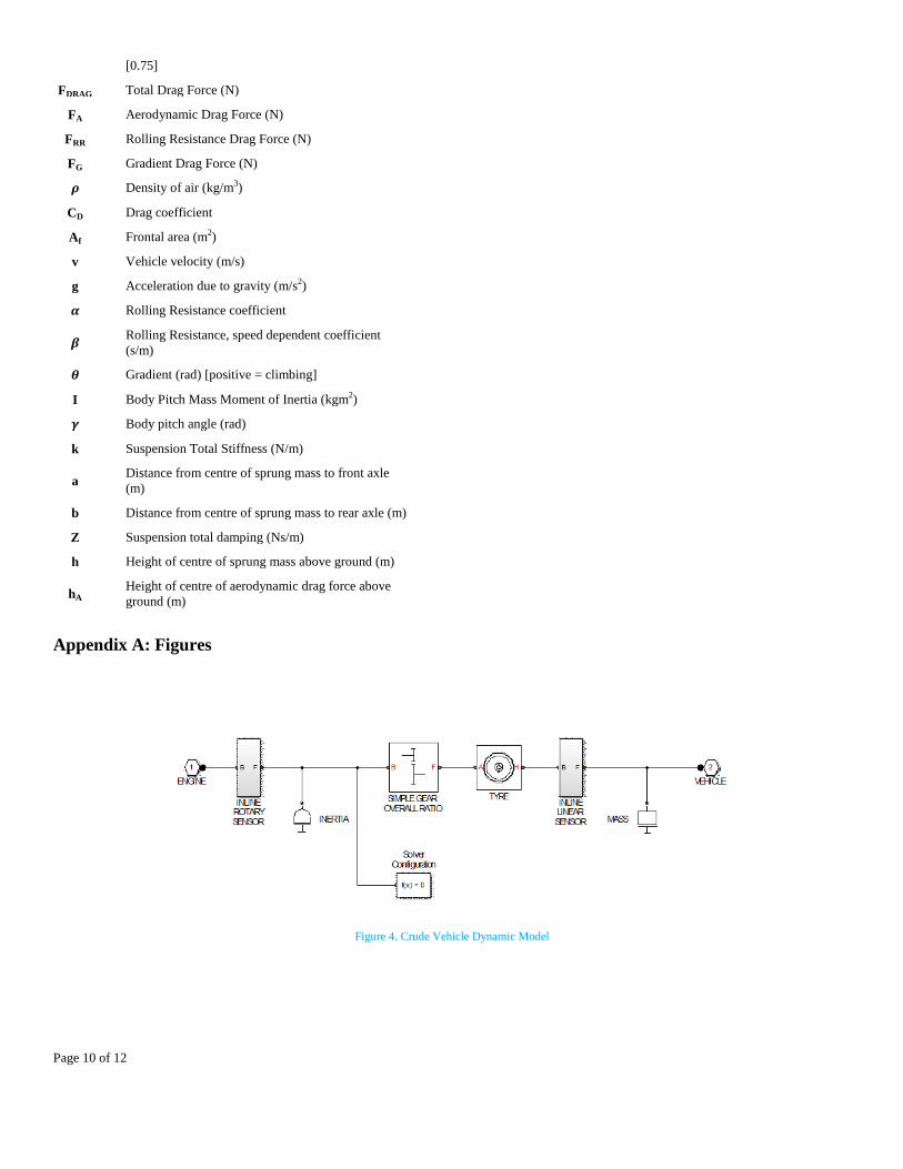
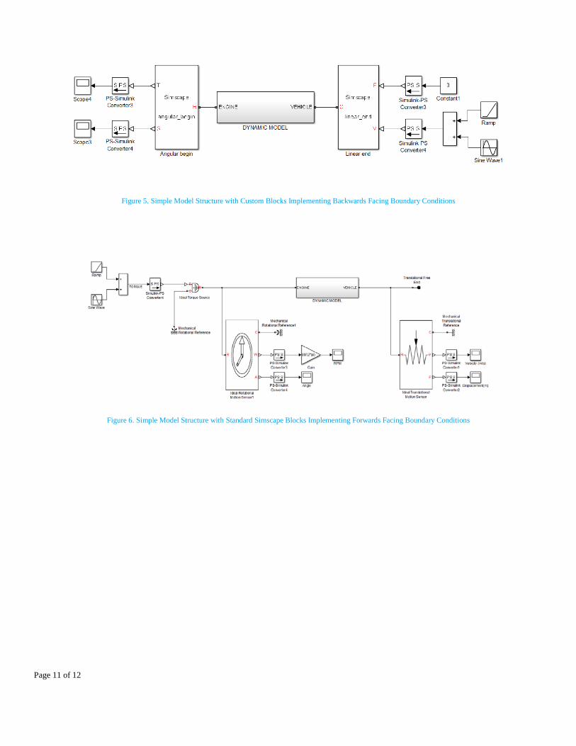
In order to demonstrate the improved modelling technique, whereby only one dynamic model is required, a simplified dynamic model was constructed. The model crudely represents a vehicle with rotational dynamics and a reduction gear representing the driveline on the left, and a mass representing the mass of the vehicle on the right. The TYRE block being the interface between the rotational and translational domains. This model is shown in figure 4.

Boundary conditions were added to the crude dynamic model, first, to create a backwards model as shown in figure 5.

Backwards simulation, as it does not correspond with a physical process is not supported by default in Simscape. Therefore, custom blocks were built which apply the correct boundary conditions, namely;

1. Imposed velocity at the vehicle body 2. Zero force at the vehicle body 3. Engine torque referred to ground 4. No constraint on engine angular velocity

This non-physically realizable set of boundary conditions forces the Simscape model to correctly represent the causality of a backwards model.

Using the same dynamic model, the boundary conditions for a forwards model were incorporated, as shown in figure 6. The appropriate boundary conditions for a forwards model are;

1. Imposed torque at the engine 2. No constraint on engine angular velocity 3. Tractive effort referred to ground 4. No constraint on vehicle linear velocity

Validation of Unified Modelling Technique

In order to validate this modelling technique, a model was constructed with a backwards model and a forwards model connected in series. The input and output values of both the through and across variables should match.

In order to provide information on the derivatives of the input signal, the Simulink to Simscape convertor block applies filtering, which adds a time delay onto the signal. In order to correctly compare model inputs with model outputs, the time delay must be included in the comparison. The parameters of the model are listed in table 4.

Table 4. Validation Model Parameters

Variable Value

Inertia 0.1 kgm2

Mass 1000 kg

Gear Ratio 10:1

Tyre Rolling Radius 0.3 m

Input torque 0.25 * t + 10 * sin (t)

Local Solver Not used

Simulink Solver Ode23t: 0.01s max sample time

of 12

The input and output torque are shown in figure 7.

Figure 7. Input and Output Torque of Validation Model

The sinusoidal component of the torque was 10 Nm while the amplitude of the torque error was 4.6x10-4 Nm, i.e., the torque error was less than 0.005%. This error is too small to be seen on the graph. The difference between input and output torque is shown in figure 8.

Figure 8. Torque Error of Validation Model

The input and output angular velocities are shown in figure 9.

Figure 9. Input and Output Angular Velocity of Validation Model

The sinusoidal component of the angular velocity was 10 rad/s while the amplitude of the angular velocity error was amplitude 6.1x10-4 rad/s, i.e., the angular velocity error was less that 0.007%. This error is too small to be seen on the graph. The difference between input and output torque is shown in figure 10.

Figure 10. Angular Velocity Error of Validation Model

The cause of the error is an offset in the timing of the input and output signals rather than a direct amplitude error. The sources of this phase error are;

1. The Simulink to Simscape input blocks optionally include a filter which causes a time delay of the input signal

2. The forwards model integrates the signal while the backwards model differentiates. These operations introduce phase changes which, ideally, should cancel.

Unified Detailed Model

The detailed vehicle model was built using MATLAB / Simscape, [1], as this tool offers advantages in modelling physical multi-domain systems, and simplifies the task of changing the fidelity of the model to suit different simulation requirements.

of 12

In this respect, Simscape is an implementation of Bond Graphs, [14], where links in the model represent an energy flow. Within each link, rather than there being one signal, there is a through variable, and an across variable. For each physical domain, the product of the through variable and the across variable gives the power (or a power like quantity). For example, in the case of mechanical translation, the through variable is the force, while the across variable is the velocity; the product of force and velocity giving power. Typical pairs of through and across variables are listed in table 5.

Table 5. Definition of Through and Across variables for physical modelling.

Domain Through Variable Across Variable

Mechanical - linear Force Velocity

Mechanical - rotation Torque Angular Velocity

Electrical Current Potential Difference

Hydraulic Flow Rate Pressure

Magnetic Flux Magneto-motive Force

Pneumatic Mass flow rate & heat flow Pressure & temperature

Thermal Heat Flow Temperature

As the links in between elements of the Simscape model represent energy flows, the direction of energy flow is determined by the conditions in each of the connected systems. Extending this idea, the energy flow in the model as a whole is therefore defined by the boundary conditions imposed upon it.

Vehicle Body and Tyre Model

As wheelspin had been identified as a potential problem for this vehicle, it was desirable to incorporate pitch plane dynamics as well as longitudinal dynamics in order to obtain an estimate of changes in drive axle loading during vehicle operation.

Along with knowledge of the dynamic drive axle load, a tyre model which incorporated a progressive slip model was required. Although it is possible to use a strongly non-linear stick-slip type tyre model, this produces numerical problems where the solver attempts to solve at the non-linear crossing point. This is alleviated by using a more progressive slip model, and as such, the simplified magic formula slip model, [15], which was used.

( ) ( )( ){ }[ ]( )υυυυ BBEBCDFFF ZZX11 tantansin, −− −−= (4)

Figure 11. Baseline Magic Formula Tyre Slip Curve

The drag force acting on the vehicle was calculated using the sum of aerodynamic drag, rolling resistance drag, and gradient drag, as written in equation (5).

( ) ( )θβαρ sin21 2 mgvmgvAC

FFFF

FD

GRRADRAG

+++=

++= (5)

The pitch plane dynamics of the vehicle were modelled as a beam rotating around a pivot located at the centre of mass with a spring and damper at each end representing the front and rear suspension.

( ) ( ) ( ) ( ) hFFhhFbaZbakI GRRAA ++−++−+−= 2222 γγγ (5)

Equations (5) and (6) were combined to produce a single custom Simscape block which takes its input from the Simscape signal representing the drive axle, and provides estimates of the vehicle’s velocity and the axle normal loads as outputs.

Engine Model

Using published data for the Opel engine used for the TC48 project, [8], a polynomial of degree four was fitted to the defined points on the torque curve. The resulting polynomial and the derived power curve are shown in figure 12.

of 12

Figure 12. IC Engine Performance Curves

The engine output was modelled using mean value data rather than time resolved engine torque simulation, in Simscape using a table lookup function.

A P+I idle speed controller was added to allow the simulation of engine idling, although in most driving modes, the engine would be shut down rather than allowing idling. The idle speed controller may be switched off for backwards modelling.

The engine’s fuel consumption was modelled using a Willan’s line estimation. Although this method does not correctly include the enrichment at high engine loads, these areas of the engine’s operating map do not form a significant part of test cycles, so this is not a serious omission.

Electric Motor Model

The electric motor performance was modelled using a 2D finite element model, from which the efficiency map was derived. The performance map was implemented using a custom Simscape block where the output of the motor was scaled with respect to supply voltage.

Battery Model

The baseline Li ion cell used for the performance simulation is the LiFeBATT XPS2E, [16]. The open circuit potential difference of one cell with respect to depth of discharge is shown in figure 13.

The battery characteristic has been implemented as a custom Simscape block where the heat loss caused by the cells’ internal resistances is calculated. Via an estimate of the cell’s heat capacity, and via a connection to a Simscape thermal network which models the heat flow via the battery pack cooling, the battery operating temperature was estimated.

Figure 13. LiFeBATT XPS2E cell open circuit potential difference [16]

Model Structure

The elements described were assembled into a Simscape model. Owing to the need to trade simulation speed for model fidelity in some modelling situations, use was made of the variant subsystem function, whereby the complexity/fidelity of the model may be selected at run time. In order that this model could be ran in both directions, the tyre slip was disabled, and the clutch was locked. The resulting model (shown in forwards configuration) is shown in figure 14.

The model, in IC engine only mode, with forwards boundary conditions was used to assess the vehicle’s acceleration performance, as shown in figure 15.

Figure 15. Vehicle Acceleration Simulation – velocity function

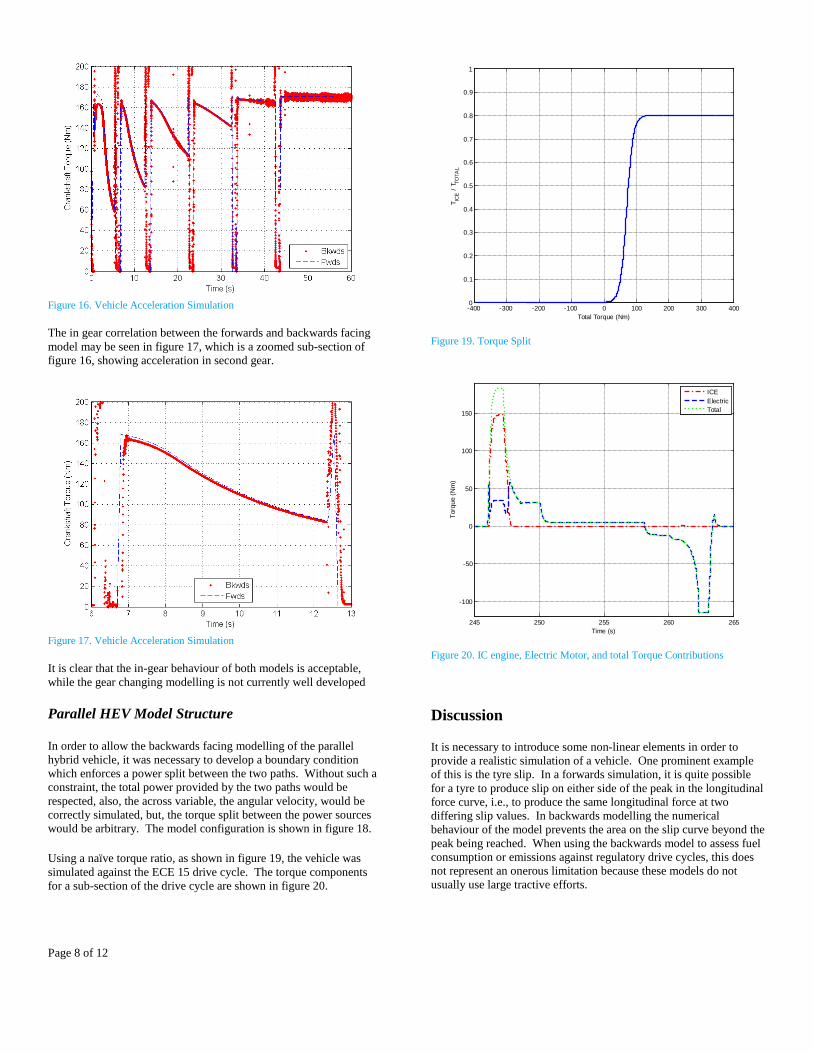
The acceleration of the vehicle was also used to assess the validity of the unified modelling technique. The comparison of the crankshaft torque required for acceleration is shown in figure 16.

of 12

Figure 16. Vehicle Acceleration Simulation

The in gear correlation between the forwards and backwards facing model may be seen in figure 17, which is a zoomed sub-section of figure 16, showing acceleration in second gear.

Figure 17. Vehicle Acceleration Simulation

It is clear that the in-gear behaviour of both models is acceptable, while the gear changing modelling is not currently well developed

Parallel HEV Model Structure

In order to allow the backwards facing modelling of the parallel hybrid vehicle, it was necessary to develop a boundary condition which enforces a power split between the two paths. Without such a constraint, the total power provided by the two paths would be respected, also, the across variable, the angular velocity, would be correctly simulated, but, the torque split between the power sources would be arbitrary. The model configuration is shown in figure 18.

Using a naïve torque ratio, as shown in figure 19, the vehicle was simulated against the ECE 15 drive cycle. The torque components for a sub-section of the drive cycle are shown in figure 20.

Figure 19. Torque Split

Figure 20. IC engine, Electric Motor, and total Torque Contributions

Discussion

It is necessary to introduce some non-linear elements in order to provide a realistic simulation of a vehicle. One prominent example of this is the tyre slip. In a forwards simulation, it is quite possible for a tyre to produce slip on either side of the peak in the longitudinal force curve, i.e., to produce the same longitudinal force at two differing slip values. In backwards modelling the numerical behaviour of the model prevents the area on the slip curve beyond the peak being reached. When using the backwards model to assess fuel consumption or emissions against regulatory drive cycles, this does not represent an onerous limitation because these models do not usually use large tractive efforts.

-400 -300 -200 -100 0 100 200 300 4000

0.1

0.2

0.3

0.4

0.5

0.6

0.7

0.8

0.9

1

Total Torque (Nm)

T ICE

/ T TO

TAL

245 250 255 260 265

-100

-50

0

50

100

150

Time (s)

Torq

ue (

Nm

)

ICEElectricTotal

of 12

Further Work

The desirable improvements in the modelling technique include developing improved estimations of the time offsets between modelling techniques, and improving the modelling of gear changing.

The custom boundary conditions have been derived for conventional vehicles, and for a parallel hybrid vehicle. These boundary conditions are to be extended to allow a broader range of vehicles to be modelled using the comined forwards facing and backwards facing method.

The custom Simscape blocks will be assembled into a library which will be made available to the community. It is further envisaged that the linear mechanical and rotational mechanical boundary conditions will be augmented by similar custom blocks which will cover the requirements of other simulation domains.

Summary

In the context of the TC48 project a means of creating a single dynamic model which can be used for both forwards and backwards modelling has been accomplished.

For a simplified linear time invariant system, the modelling technique has shown errors in torque and angular velocity of less than 0.01% which is comfortably less than typical uncertainties in vehicle parameters, and is therefore acceptable for use in the TC48 project.

Where the model contains elements which vary with respect to time, such as the gear ratio in an automotive transmission, discrepancies have been identified, and further work has been identified.

References

1. Mathworks, “Simscape,” 3.11, http://www.mathworks.co.uk/help/physmod/simscape/index.html.

2. Mathworks, “Simulink,” 8.3, http://www.mathworks.co.uk/help/simulink/.

3. 48V Town & Country Hybrid Powertrain, http://www.tc48.co.uk/, Oct. 2014.

4. Kuypers, M., “Application of 48 Volt for Mild Hybrid Vehicles and High Power Loads,” Society of Automotive Engineers, 2014, doi:10.4271/2014-01-1790.

5. Alexander, D.G. and Blackketter, D.M., “Eliminating the Forward / Backward Restriction in Vehicle Performance and Energy Use Analysis,” (724), 2014.

6. Miller, T.J.E., “Switched Reluctance Motors and their Control,” Oxford University Press, 1993.

7. Dong, G., Han, X., Stobart, R., and Lu, S., “Dynamic Analysis of the Libralato Thermodynamic Cycle Based Rotary Engine,” 2013, doi:10.4271/2013-01-1620.

8. Opel presents new 1.0 SIDI Turbo engine, http://www.opel.com/news/index/2013/10/Opel_presents_new_1-0_SIDI_turbo_engine.html, Oct. 2014.

9. Marco, J., Ball, R., and Jones, R.P., “The Design of a Parallel Hybrid Transmission Control System,” in: Vaughan, N. D., ed., Integrated Powertrains and their Control, Professional Engineering Publishing, 2000.

10. Lucas, G.G., “Road Vehicle Performance,” 1st ed., Gordon and Breach, 1986.

11. Guzzella, L., and Sciarretta, A., “Vehicle Propulsion Systems: Introduction to Modeling and Optimization,” Springer, 2012.

12. Guzzella, L. and Amstutz, A., “The QSS Toolbox Manual,” (June), 2005.

13. Lechner, G,, and Naunheimer, H., “Automotive Transmissions: Fundamentals, Selection, Design and Application,” Springer, 1999.

14. Cellier, F. E. and Greifeneder, J., “Continuous System Modeling,” 1st ed., Springer, 1991.

15. Pacejka, H., “Tire and Vehicle Dynamics,” 3rd ed., Butterworth-Heinemann, 2012.

16. LiFeBATT, “LiFeBATT- XPS2E,” 3–6, http://www.lifebatt.com/new2/XPS2ECellSpecifications.pdf.

Acknowledgments

This project was co-funded by Innovate UK, the UK’s innovation agency. The authors wish to thank Innovate UK and the other contributing members of the TC48 project consortium : http://www.TC48.co.uk

Definitions/Abbreviations

𝝋 𝟏 Base Ratio Step

𝝋 𝟐 Gear Ratio Progression Factor

r Gear Ratio (reduction)

Z Number of selectable ratios

N Index number of selected gear (1 = 1st, 2 = 2nd, …)

T Simulation time (s)

Fx Tyre Longitudinal Force (N)

Fz Tyre Vertical Force (N)

𝝂 Tyre Slip

B Stiffness coefficient in simplified magic formula [7]

C Shape coefficient in simplified magic formula [1.9]

D Peak coefficient in simplified magic formula [0.7]

E Curvature coefficient in simplified magic formula

http://www.tc48.co.uk/

of 12

[0.75]

FDRAG Total Drag Force (N)

FA Aerodynamic Drag Force (N)

FRR Rolling Resistance Drag Force (N)

FG Gradient Drag Force (N)

𝝆 Density of air (kg/m3)

CD Drag coefficient

Af Frontal area (m2)

v Vehicle velocity (m/s)

g Acceleration due to gravity (m/s2)

𝜶 Rolling Resistance coefficient

𝜷 Rolling Resistance, speed dependent coefficient (s/m)

𝜽 Gradient (rad) [positive = climbing]

I Body Pitch Mass Moment of Inertia (kgm2)

𝜸 Body pitch angle (rad)

k Suspension Total Stiffness (N/m)

a Distance from centre of sprung mass to front axle (m)

b Distance from centre of sprung mass to rear axle (m)

Z Suspension total damping (Ns/m)

h Height of centre of sprung mass above ground (m)

hA Height of centre of aerodynamic drag force above ground (m)

Appendix A: Figures

Figure 4. Crude Vehicle Dynamic Model

of 12

Figure 5. Simple Model Structure with Custom Blocks Implementing Backwards Facing Boundary Conditions

Figure 6. Simple Model Structure with Standard Simscape Blocks Implementing Forwards Facing Boundary Conditions

of 12

Figure 14. Detailed Model - Forwards Facing Boundary Conditions

Figure 18. Detailed Model – Backwards Facing Boundary Condition

unified backwards facing and forwards facing simulation of

Documents