Uniform Price Mechanisms for Threshold Public Goods Provision with Private Value Information: Theory and Experiment

Zhi Li*, Christopher Anderson†, and Stephen Swallow‡

Abstract

This paper compares two novel uniform price mechanisms for provision point public goods to

standard provision point (PPM) and proportional rebate (PR) mechanisms within a Bayesian

game with private value information. The uniform price auction mechanism (UPA) collects an

endogenously determined uniform price from everyone offering at least that price, while the

uniform price cap mechanism (UPC) collects the uniform price from everyone offering at least

that price, plus the full offer of everyone offering less. By rebating full amounts in excess of the

price, the uniform price mechanisms create regions where the expected increase in payment

associated with a higher offer is zero. We show that the uniform price mechanisms support

Bayesian Nash equilibria (BNE) with higher contributions than BNE of PPM or PR, potentially

increasing efficiency. We use laboratory experiments to test whether these more efficient BNE

obtain, leading to higher contributions or more frequent provision. Our mechanisms outperform

PR and PPM with private values: UPC generates higher aggregate contributions and provision

rates than PR and PPM; UPA attracts much higher contributions, although it provides less

frequently. This ranking emerges because high offers are more common (especially among high-

value people) in the uniform price mechanisms, where it is low cost to venture high offers to

potentially meet other high offers to support provision.

Keywords: Uniform price auction, Uniform price cap, Proportional rebate, Provision point

mechanism

* Department of Economics, University of Washington † School of Aquatic and Fishery Sciences, University of Washington ‡ Center for Environmental Sciences and Engineering and Department of Agricultural and Resource Economics, University of Connecticut.

1

1. Introduction

The provision point mechanism (PPM) for public goods provision is one where the good can be

provided only if a threshold level of funding contributions is met. After Bagnoli and Lipman

(1989) showed that the equilibrium outcome is always efficient in undominated perfect equilibria

with complete information, it has been systematically studied, both theoretically1 and

experimentally2. PPM’s popularity in the economics literature can be attributed to the fact that

many public goods have an inherent threshold or discrete nature for provision, such as parks,

public radio broadcasting, and environmental conservation projects, where a minimum amount

of funding is needed to provide one unit. The PPM requires only a slight modification—addition

of the provision point—to the common open-ended donation solicitation used by charities, and

hence many fundraisers use the PPM due to its simplicity and support for provision in

equilibrium.3

One practical problem with the PPM is how to deal with the contribution in excess of the

provision cost, attributable to a combination of incomplete value information and imperfect

coordination within the continuum of efficient Nash equilibria. Without rebate, contributors may

view the extra money as wasted, potentially creating a disincentive for contribution in the first

place, and especially discouraging high offers. However, rebating extra money provides an

opportunity to shift the off-path incentives of the PPM, and perhaps attract additional

contributions: this has led to an additional literature on whether and how different methods for

rebating contributions in excess of the provision cost affect contributions. The most popular

rebate rule is the proportional rebate (PR), which rebates the extra contribution in proportion to

the ratio of an individual’s contribution to the total contribution.

4

1 Bagnoli and Lipman (1989) study PPM under complete information; Nitzan and Romano (1990), McBride (2006), and Barbieri and Malueg (2010a) discuss threshold uncertainty; Alboth et al. (2001), Menezes et al. (2001), Laussel and Palfrey (2003), and Barbieri and Malueg (2008, 2010b) discuss PPM with private value information.

The results in the experimental

literature are mixed: Marks and Croson (1998) find no significant difference between PPM and

PR under complete information, while Gailmard and Palfrey (2005) find PR (called PCS in their

paper) generates significantly higher contributions than PPM when value information is private.

Only a few of the possible factors affecting these mixed results have been explored (Rondeau et

al.,1999; Rondeau et al, 2005; Spencer et al., 2009).

2 See Chen (2008) for a recent review of related experimental studies; for earlier reviews see Davis and Holt (1993) and Ledyard (1995). 3 See real world examples in Bagnoli and Mckee (1991) and Marks and Croson (1998), or www.kickstarter.com. 4 Marks and Croson (1998) and Gailmard and Palfrey (2005) provide comprehensive references on PR.

2

To provide a coherent framework for understanding how rebate rules affect contributions

and also to improve upon PPM and PR, Li et al. (2014) introduce two novel uniform price

mechanisms, the uniform price auction mechanism (UPA) and the uniform price cap mechanism

(UPC). In UPA, everyone who pays, pays the same price: if there exists a price such that the

number of contributions at or above that price multiplied by the price equals the provision point,

then the good is provided, with only those offering at or above the uniform price paying the

uniform price; the lowest such price will be chosen if more than one uniform price is possible.

UPC addresses an inefficiency inherent in UPA, that contributions can exceed the provision cost,

but still no uniform price meeting the provision rule exists. In UPC, no one pays more than the

uniform price: if the provision point is exceeded, the lowest price cap will be calculated so

whoever contributes above the cap pays only the cap, and those contributing less than the cap

pay their full offer, such that the final collected payments equal the provision point.

The objective of the uniform price mechanisms is to design a rebate rule that induces

higher overall contributions by alleviating participants’ concern that contributing more to support

provision may lead to losing more of the (over)contribution in the event of provision. This

extent of concern is measured by the “marginal penalty,” the cost of contributing an additional

dollar conditioned on provision (Marks and Croson, 1998). In a true PPM, all overcontribution

is wasted so the marginal penalty is -1, and in PR the marginal penalty is between -1 and 0. The

two uniform price mechanisms, on the other hand, have a wide range of aggregate contributions

where the marginal penalty is zero, and therefore they are expected to induce higher

contributions. Through lab experiments, Li et al. (2014) find that the uniform price mechanisms

do outperform PPM and PR under complete information. The insight is that the lower marginal

penalty facilitates equilibrium selection by making it safer to tender higher offers, and therefore

the uniform price mechanisms lead to higher contributions and more frequent provision.

A key feature missing in the application of these mechanisms in a complete information

game is that the rebate is irrelevant in equilibrium, since excess contributions never occur in

equilibrium,5

5 Bagnoli and Lipman (1989) show in undominated perfect equilibria, the provision point is exactly met in PPM; and Li et al. (2014) verify that PR and UPC have the same set of undominated perfect equilibria as PPM.

so equilibrium theory is silent about how different rebate rules may affect the

contribution behavior. In a Bayesian framework, however, excess contributions can occur when

3

a value profile with higher-than-expected induced values is realized, and therefore the role of

rebates can be explored by comparing the equilibria of each mechanism.

This paper first elucidates how the alternative rebate rules affect the expected payoff

function by examining the expected marginal penalty associated with higher offers in each

mechanism. We then characterize the Bayesian Nash equilibria (BNE) of the two uniform price

mechanisms, and compare the equilibrium sets with those of PPM and PR in an incomplete

information setting. With an almost always zero-expected marginal penalty, UPA has a truth-

telling BNE in a 2-player game, and depending on parameters, may support BNE where the

expected group contribution is close to (more than 90% in our examples) the total expected

induced value in a game with 3 or more players. UPC has a BNE characterization similar to

PPM and PR as shown in Gailmard and Palfrey (2005). By a numerical example, we find

rebates induce some BNE with higher contributions from high-value types: PR and UPC

generate contributions comprising equilibria more efficient than PPM, and UPC induces higher

contributions from high-value people than PPM and PR. These rebates work by reducing the

expected payment cost for high-value people more than low-value people, since high-value

people are more likely to face a value profile with higher-than-expected induced values and

hence will experience overcontribution with a higher probability and pay more of the excess

contribution in the absence of a rebate. Further, UPC has a marginal penalty structure that

reduces the overcontribution cost more effectively than PR by only protecting high contributors:

all excess contributions in UPC are returned to those contributing higher than the price-cap who

are generally high-value people (as shown in Proposition 2 below). These theoretical predictions

are supported by our experimental results: UPC generates higher aggregate contributions and

provision rates than PR and PPM; UPA attracts much higher contributions, although it provides

less frequently.

The rest of the paper is organized as follows. Section 2 defines precisely the four

mechanisms to be compared, and analyzes the effect of their respective marginal penalty

structures on their expected payments. Section 3 characterizes the BNE sets of UPA and UPC,

demonstrates differences in the mechanisms’ BNE sets with numerical examples, and explains

the underlying role of marginal penalty in differentiating the sets of equilibria. Section 4

describes the experimental design and procedures. Section 5 discusses the observed group and

individual contributions. Section 6 synthesizes these results.

4

2. The Mechanisms and Their Marginal-Penalty-Structure Effect on the Expected Payment

Suppose N agents each have endowment I. Each simultaneously chooses to make a contribution

ci to the provision of a threshold public good with a cost of PP. If the public good is provided,

each agent receives a private value of vi independently drawn from a common knowledge value

distribution. If the public good is not provided, all contributions are refunded (money-back

guarantee).

2.1 Provision Point Mechanism (PPM)

The payoff function for agent i under PPM is

(1)

Under PPM, if PP is met or exceeded, each agent receives the initial endowment I minus their

contribution ci, plus their private value, vi, for the public good; otherwise, they only get I.

If contributions exceed PP, PPM “burns” the excess. Alternatively, excess contributions

can be returned through rebate mechanisms, which may affect contribution strategies. PR, UPA,

and UPC return excess contributions in different ways.

2.2 Proportional Rebate (PR)

Agent i’s payoff under PR is

(2)

Under PR, if , the excess contribution ( ) will be rebated. The rebate to

each agent is proportional to the ratio of their individual contribution to the total contribution.

2.3 Uniform Price Auction (UPA)

Under UPA, a uniform price, UP, will be calculated. UP is the lowest price such that the number

of contributions higher than that price times the price is equal to PP. The payoff under UPA is

(3)

1

1

+ , ,

+ , ,

π

=

=

≥ ≠ ∅ <= − ≥ ≠ ∅ ≥

∑∑

Ni j ij

Ni i j ij

I v if c PP UP and c UP

I UP v if c PP UP and c UP

I otherwise

. If an agent contributes less than UP, she pays

nothing and the full ci will be rebated. If an agent contributes UP or more, she will pay only the

1

π =

− + ≥=

∑Ni i jj

i

I c v if c PP

I otherwise

( )1 1

1

π = =

=

− + + − ≥=

∑ ∑∑

N Nii i j jN j j

ji j

cI c v c PP if c PPc

I otherwise≥∑ jj

c PP −∑ jjc PP

5

price UP and the excess contribution will be rebated. To provide the good, UPA requires not

only that the total contribution meet or exceed PP, but also that the number of relatively high

individual contributions be sufficient. More precisely, PP and the group size together determine

a set of at most N possible prices, where PP is shared by n≤N agents offering at least PP/n. If the

contributions in aggregate exceed PP, but cannot satisfy np=PP for some n, the mechanism does

not provide; with such an outcome, UPA is not efficient.

2.4 Uniform Price Cap (UPC)

UPC is a modified version of UPA that ensures the good can be provided whenever total

contributions exceed PP. The payoff under UPC is

(4)

where { : }

min{ 0 : , { : }}∈ <

= > + = = ≥∑k

j ij k c pUC p c np PP n i c p . Under UPC, if there are

excess contributions, a uniform price cap (UC) will be calculated. If an agent contributes less

than UC, she pays her full contribution ci (under UPA she would have paid nothing). If an agent

contributes UC or more, she pays only the price cap and the excess contribution is rebated, just

like under UPA. UC is calculated as the lowest price that could collect exactly PP. Since

contributions lower than the price will not be rebated, the uniform cap UC always exists as long

as contributions at least meet PP; with such an outcome, UPC is efficient.

2.5 The Effect of Marginal Penalty of Overcontribution on the Expected Payment

Marks and Croson (1998) use the concept of marginal penalty—the private payoff loss

associated with an additional unit of contribution, conditioned on provision—to argue that rebate

rules reduce the cost of making higher private offers in the absence of coordinating on a single

equilibrium in their complete information game, increasing aggregate contributions and the

likelihood of provision. It is insightful to translate their concept to an ex ante expected marginal

penalty in our Bayesian framework, in order to better understand how rebate rules can influence

BNE. Crucially, in a Bayesian game, a profile with high value-realizations will generate excess

contributions in equilibrium, meaning the effect of lower marginal penalties can be identified

within the equilibrium concept, as mechanisms with lower marginal penalties may support

strategy profiles with higher contributions as equilibria.

1

1

+

π=

=

− ≥ <= − + ≥ ≥

∑∑

Ni i j ij

Ni i j ij

I c v if c PP and c UC

I UC v if c PP and c UCI otherwise

6

To understand the marginal penalty associated with each of our mechanisms, we examine

the expected payoff function, conditioned on others’ strategies, of a 2-player Bayesian game with

continuous types. Each agent has an induced value iv , i=1, 2, independently drawn from [ , ]v v

with a pdf ( ) 0, [ , ]> ∀ ∈i if v v v v , where ( 2 , )∈v PP PP to make a collective contribution

necessary for provision. Without loss of generality, we discuss agent 1’s expected payoff,

conditioned on agent 2’s contribution function 2 ( )⋅c of 2v . For simplicity, we assume 2 ( )⋅c is

strictly increasing and differentiable over [ , ]v v and we omit the endowment I in the expected

payoff function.

In PPM, agent 1’s expected payoff of contributing 1c conditioned on 1v and 2 ( )⋅c is

(5) 1 1

2 2 1 2 2 11 1 1 2 1 2 2 1 2 2( ) ( )

( | , ( )) ( ) ( ) π− −≥ − ≥ −

⋅ = ⋅ − ⋅∫ ∫PPM

v c PP c v c PP cE c v c v f v dv c f v dv ,

where the integrations represent the probability of provision, and the two terms on the RHS are

the expected benefit and cost, respectively. Take the derivative of (5) w.r.t. 1c , we have

(6) ( )( ) 1

2 2 1

12 11 1 1 2

1 1 2 21 ( )1 2 2 1

( )( | , ( )) ( ) 1 ( ) ( )

π−

−

− ≥ −

−∂ ⋅= − ⋅ − ⋅

∂ ′ − ∫PPM

v c PP c

f c PP cE c v c v c f v dvc c c PP c

On the RHS of (6), the first term represents the marginal net benefit due to an increased

provision probability from a higher contribution. The second term, which is the one we are

looking for, is the expected marginal penalty of overcontribution: it says given the same

provision probability (the lower bound of the integration is unchanged), if 1c increases by 1, the

cost also increases by 1 (the integrand) conditioned on provision, reflecting a -1-marginal penalty

in PPM. Rebates and hence a lower marginal penalty reduce ex ante this expected marginal

penalty cost.

In PR, given the same 2 ( )⋅c , we have

(7) 1 12 2 1 2 2 1

11 1 1 2 1 2 2 2 2( ) ( )

1 2 2

( | , ( )) ( ) ( ) ( )

π− −≥ − ≥ −

⋅⋅ = ⋅ −

+∫ ∫PR

v c PP c v c PP c

c PPE c v c v f v dv f v dvc c v

(8) ( )( ) 1

2 2 1

12 11 1 1 2 2

1 1 2 221 ( )1 1 22 2 1

( )( | , ( )) ( )( ) ( ) ( ( ))( )

π−

−

− ≥ −

−∂ ⋅ ⋅= − ⋅ − ⋅

∂ +′ − ∫PR

v c PP c

f c PP cE c v c PP c vv c f v dvc c c vc c PP c

Compared to (6), the only difference in (8) is the integrand on the RHS, which is the marginal

penalty in PR (exactly the same as defined in Marks and Croson, 1998). Note that the marginal

7

penalty is bounded between -1 and 0, almost always greater than -1, and becomes closer to 0 as

1c increases. Given 1c and 2 ( )⋅c , the expected marginal penalty in PR is less than that in PPM,

especially for higher contributors, and hence higher contributions may be supported in

equilibrium in PR, consistent with Marks and Croson.

Our uniform price mechanisms aim to increase contributions by creating regions of zero-

marginal penalty, which result in even lower expected payments. In a 2-player game of UPA,

the good is provided only if both agents contribute PP/2 or above and each pays PP/2, so

(9) 1 1

2 2 2 2

1

1 1 1 21 2 2 2 2 1( 2) ( 2)

0 2 ( | , ( ))

( ) ( ) 22

π− −≥ ≥

<⋅ =

⋅ − ⋅ ≥ ∫ ∫UPA

v c PP v c PP

if c PPE c v c PPv f v dv f v dv if c PP

Compared to (5) and (7), the expected payoff in UPA is independent of 1c within [0, PP/2) and

[PP/2, PP). Since agent 1 pays either 0 or PP/2, the marginal penalty is always 0 except at PP/2

across which the payment jumps from 0 to PP/2. Thus, the expected marginal penalty is always

zero except at PP/2, where the expected payment is (PP/2)1

2 22 2( 2)

( ) −≥∫v c PP

f v dv . More generally

in an N-player game (N>2), as shown in Li et al (2014), if c1<UP(c1|c-1) where UP(c1|c-1) is the

uniform price that provides the good through payments of PP/m by m other agents, there exists a

cutpoint, ∈(c1, UP(c1|c-1)) at which agent 1’s contribution is sufficient to be included in

payments of the next lowest uniform price, and the final payment jumps from 0 to the new price,

UP( |c-1)= PP/(m+1). Then, the marginal penalty of UPA is zero almost always, except at

the cutpoint with a lump sum penalty, resulting in an expected marginal penalty structure similar

to the 2-player case. Given the broad range of values with no expected marginal penalty, we

conjecture higher contributions in UPA than the other mechanisms.

In UPC, the uniform cap is PP–c1 when c1<PP/2, and is max{PP–c2(∙), PP/2} when

c1≥PP/2, so we have

(10)

1 12 2 1 2 2 1

12

1 12 2 1 2 1

12 2

1 2 2 1 2 2 1( ) ( )

( 2)1 1 1 2

1 2 2 2 2 2 2( ) ( )

2( 2

( ) ( ) 2

( | , ( )) ( ) [ ( )] ( )

( )2

π

− −

−

− −

−

≥ − ≥ −

≥ − −

≥

⋅ − ⋅ <

⋅ = ⋅ − −

− ⋅

∫ ∫

∫ ∫

v c PP c v c PP c

UPC c PP

v c PP c c PP c

v c PP

v f v dv c f v dv if c PP

E c v c v f v dv PP c v f v dv

PP f v 2 1) 2

≥ ∫ dv if c PP

8

(11)

( )( )

( )( )

12 2 1

12 1

1 1 2 2 11 ( )2 2 1

1 1 1 2

1 12 1

1 1 112 2 1

( )( ) 1 ( ) 2

( )( | , ( ))

( )( ) 2

( )

π

−

−

− ≥ −

−

−

−− − ⋅ <

′ −∂ ⋅ = ∂ − − > ′ −

∫v c PP cUPC

f c PP cv c f v dv if c PP

c c PP cE c v c

cf c PP c

v c if c PPc c PP c

UPC has a hybrid expected payoff structure of PPM (5) and UPA (9). Thus, when c1<PP/2,

UPC has the same expected marginal penalty 1

2 2 12 2( )

1 ( ) −≥ −

− ⋅∫v c PP cf v dv as PPM. When c1>PP/2,

UPC has a zero-expected marginal penalty, similar to UPA: the expected marginal cost of

increasing 1c is only due to the increased provision probability while not the marginal penalty of

overcontribution (i.e., a zero-marginal penalty). At c1=PP/2, the expected marginal penalty is

not defined. It is easy to verify that, in an N-player game (N>2), if c1 is at or above UC(c1|c-1),

the uniform cap that provides the good as a function of c1 given c-1, then any incremental

contribution will not change the cap, creating a marginal penalty of 0. If c1<UC(c1|c-1), there

exists a cutpoint, , at which the marginal penalty changes from -1 to 0 ( =PP/2 in a 2-

player game). Hence, UPC generally has a zero-expected marginal penalty when the individual

contribution is high enough,6

In contrast to in a complete information game where PPM, PR, and UPC have the same

Pareto efficient equilibrium set, in Bayesian games these expected marginal penalties do

differentiate the mechanisms’ equilibrium sets and provide theoretical benchmarks for further

experimental comparisons, as shown in the next section.

and based on beliefs about c-1, agents calculate an expected

marginal penalty between -1 and 0. Compared to PPM and PR, UPC may induce even higher

contributions bearing in mind that the major excess offer would be from high contributors.

3. Bayesian Nash Equilibria

To proceed, we focus on Bayesian games with discrete types.7

6 Intuitively, this is due to our design of UPC to focus on protecting high contributors: the excess offer is only rebated to those contributing above the cap, in contrast to PR where all contributors share the excess offer.

We first characterize some basic

properties of the BNE sets of UPC and UPA as Gailmard and Palfrey (2005) do for PPM and PR.

7 Although the role of rebates and the corresponding marginal penalty structure can be clearly revealed in a continuous-type analysis, these mechanisms except for UPA are much more difficult to analyze with private value information and continuous types: there is only a small body of literature on PPM (Alboth et al., 2001; Menezes et al., 2001; Laussel and Palfrey, 2003), and even no analysis on PR. Solving PR or UPC alone may need a full-length paper. On the other hand, it is easier to solve numerically a game with discrete types without losing the key insights

9

Then we solve for symmetric BNE of UPA in a 3-player game and discuss the general BNE

solution structure and the value revelation property of UPA in an N-player game. Lastly, we

differentiate the BNE sets of the four mechanisms using a numerical example.

3.1 Basic Properties of the BNE sets of UPC and UPA

Following the model setup in the beginning of Section 2, agent i ’s induced value iv is

independently drawn from a finite set V of real numbers with a common knowledge probability

distribution function. V is the same for all agents. We assume , so, as in

the interesting (and challenging real) context, provision is not optimal for any individual. All

above information is common knowledge except that the realized iv is only known to agent i .

Let 1( , , )= … ∈ NNv v v V denote a profile of values, 1 1( ) ( ( ), , ( ))= … N Nc v c v c v denote a

contribution strategy profile with one contribution function for each agent, and

1 1 1 1( , , , , )− − += … …i i Nv v v v v and similarly for 1 1( )− −c v . Further, let |( )−i i iP c c denote the

provision probability when agent i contributes ic given the contribution functions of the others,

let ( ( ))is c v denote agent i ’s final payment as a function of ( )c v , and let

( ) ( ( ( )) | )−

=ii i v i iS c E s c v c denote i ’s expected payment given contribution ic .

Gailmard and Palfrey (2005) present three common properties of the BNE sets of PPM

and PR: no overbidding, payment monotonicity and contribution monotonicity. We show that

the BNE sets of UPC and UPA have three similar properties with some regularity conditions.

Proposition 1 (No overbidding). In UPC, any strategy in which ( ) >i i ic v v for some iv is ex

post weakly dominated; in UPA, any strategy in which ( )i ic v is greater than the lowest

/ ≥ iPP k v for {1, , }∈ …k N and some iv , is ex post weakly dominated.

Proof: See Appendix.

Lemma 1 (Payment monotonicity). In UPC, if |( ) 0− >i i iP c c and ic is less than PP and the

cutpoint associated with some uniform cap for some value profile v , ( )i iS c is strictly

increasing at ic ; in UPA, if |( ) 0− >i i iP c c and ic is less than PP and the cutpoint

about the mechanisms, as Gailmard and Palfrey (2005) do for PPM and PR. Therefore, we will focus on discrete types in the following sections of the paper.

10

associated with some uniform price for some value profile v , ( )i iS c is strictly increasing at ic in

the sense that when ic increases to a higher uniform price, ( )i iS c increases.

Proof: See Appendix.

Note that the cutpoints and are defined as in Section 2.5.

Proposition 2 (Contribution monotonicity). For both UPC and UPA, let * ( )c v be a symmetric

Bayesian Nash equilibrium contribution function.8 * *|( ( ) ) 0− >i iP c v c If for all min{ }>v V and

*( )c v is less than the cutpoint associated with some uniform cap/price for some value profile v ,

then, for all iv and jv , * *( ) ( )> ⇒ ≥i j i jv v c v c v .

Proof: See Appendix.

The three properties of UPC are exactly the same as those of PPM and PR, except for the

additional regularity condition that ic or *( )c v is less than the cutpoint associated with some

uniform cap for some value profile v . This regularity condition eliminates the uninteresting and

extremely rare cases that ic or *( )c v is always greater than any possible uniform cap for all

value profiles; in these rare cases ( )i iS c is only weakly increasing at ic . In addition to a similar

regularity condition, the properties of UPA in Proposition 1 and Lemma 1 are restated to reflect

the step-function form of the payment scheme, since in UPA realized payments can only be one

of a finite number of uniform prices. With these adjustments, the proofs of the properties of

UPC and UPA are similar to those for PR in Gailmard and Palfrey (2005).

These regularity conditions reflect some additional properties of UPC and UPA due to

their marginal penalty structure. Next, we use symmetric BNE of UPA to show its advantage in

generating higher contributions, and then demonstrate how UPC results in BNE sets different

from PPM and PR and discuss the underling incentives.

3.2 Symmetric BNE of UPA

Since there are only finite possible prices in UPA, it is equivalent to a Bayesian game with

discrete actions. It is known that a BNE solution to this kind of game has the form of a decision

rule based on some critical values. Therefore, we can solve the Bayesian game for UPA by

8 We abuse the notations here and in the following discussions to emphasize the symmetry: v and are both scalars, representing one agent’s value and equilibrium contribution strategy.

11

identifying the decision rules and the critical values. We will solve for symmetric BNE of UPA

in a 3-player game first, and discuss the general BNE solution structure in an N-player game.

Without loss of generality, we assume agents only contribute the possible uniform prices.

In a 3-player game, each agent has three contribution choices {0, PP/3, PP/2} and two critical

values will be enough to characterize the decision rule. Let 3cv and 2

cv denote the two critical

values for a symmetric pure-strategy weakly monotonic BNE, assuming 230 ≤ ≤ ≤c cv v v , where

0 min{ }= V and max{ }=v V . The contribution function for each agent is in the general form

(12) 2

3

2

3

0

( ) 3 <

2

≤

= ≤ >

c

c c

c

if vc v PP if v

PP vif v

vv v

Then the BNE of UPA in the 3-player game are as follows.

Proposition 3. In a 3-player Bayesian game, UPA has the following four categories of

symmetric BNE: for i = 1, 2, 3,

a) ( ) 0=BNEi ic v , with 23 = =c cv v v .

b) 0 3

( ) 3 3

≤= >

iBNEi i

i

if v PPc v

PP if v PP, with 3 3=cv PP and 2 =

cv v .

c) ˆ 0

( )ˆ 2

≤= >

iBNEi i

i

if v vc v

PP if v v,

with 3 2ˆ 2> = = >c cv vv v PP and v̂ given by ˆ( 3)v PP− ˆPr( )v v> ˆ( 2)v PP= − .

d) 3

3

0

( ) 3 < 2 2 2

≤

= ≤ >

iBNEi i i

i

c

c

if vc v PP if v PP

PP if v PP

vv ,

with 32 2 3= > >c cPP v PPv and 3cv given by 3 3

2 22 3Pr( ) ( 3) Pr( )> = − >c c c cv v v vv PP v .

Proof: See Appendix.

Note that ˆPr( )>v v denotes the probability of ˆ>v v . Similarly for 2Pr( )> cvv and 3Pr( )> cvv .

Remark 1. Given our parameter assumption that ( )max{ } 3,∈V PP PP , solutions a and

b always exist. The existence of c and d requires additional conditions on PP, v , and the value

distribution. First, PP should be less than 2v , otherwise PP/2 is not a feasible price. Also, PP

12

should be high enough relative to v to support c and d (especially for d). We use a uniform

value distribution over [0, 1] to demonstrate these additional conditions in the appendix.9

Remark 2. A “category” of symmetric BNE in UPA includes all the contribution

strategies that are equivalent to a symmetric BNE where only the possible uniform prices are

used as contribution choices, as one of the listed BNE in the proposition. For example, any

strategy with individual contributions always below PP/3 is a symmetric BNE in category a,

since contributing below PP/3 is equivalent to contributing 0. Because these small contributions

cannot affect payments, reflecting the zero-marginal penalty structure, they cannot be excluded

as equilibria. This feature advantages UPA in value revelation: in d, agents can reveal their true

values without affecting their payments over the entire value range except for the interval [PP/3,

3cv ] where agents need to contribute less than PP/3 to follow the equilibrium strategy.

Generally, a BNE including more of the feasible uniform prices (d with two positive

prices vs. c with only one) supports a larger truth-telling value range: b to d all support larger

truth-telling value ranges than a (i.e., the non-truth-telling ranges of [PP/2, v ], [PP/2, v̂ ] and

[PP/3, 3cv ] are all smaller than [PP/3, v ]); the comparisons among b to d depend on parameters.

We show in the appendix that d, if it exits, has the largest truth-telling range. In the special case

of a two-player game, truth-telling over the entire value range is supported in UPA as agents

contribute PP/2 when and 0 otherwise (See Appendix).

In an N-player game, UPA has a solution structure similar to that in the 3-player game,

which is summarized in the following proposition.

Proposition 4. In an N-player Bayesian game, assuming ( )max{ } ,∈V PP N PP ,

• UPA always has the following two categories of symmetric BNE: for i = 1, …, N,

e) ( ) 0=BNEi ic v , for all ∈iv V .

f) 0

( )

≤= >

iBNEi i

i

if v PP Nc v

PP N if v PP N

• BNE with uniform prices higher than PP/N and/or with more than one uniform price may or

may not exist, depending on whether the corresponding critical values can be identified from

9 These BNE also apply to a game with continuous types.

13

a system of polynomial equations given the parameters of PP, V and the value distribution.

The BNE with the most numerous different prices, if it exits, is

g) ,

with 2 2= > >kc cvPv P PP k , for k = 3, …, N, and the critical values are given

by a system of N-2 polynomial equations.

Proof: See Appendix.

The general procedure to solve the N-player game and the general form of the expected payoff

function at each possible uniform price used to construct the system of polynomial equations are

given in the appendix.

Remark 3. Although it is not incentive compatible in general (cf. Borgers et al., 2015),

UPA may still support relatively high value revelations for pure public goods due to the same

reason discussed in Remark 2, in contrast to the direct serial cost sharing mechanism (Moulin,

1994) where incentive compatibility is obtained only for excludable public goods.10

10 If we have in equilibrium

Therefore,

we would expect relatively high contributions in UPA even in BNE. Note that this value

revelation property is primarily due to the step-function style of payment scheme, which is fully

captured by the almost always zero-expected marginal penalty structure. Also, the equilibrium f

of UPA results in the same equilibrium outcome as the “conservative equal-costs” mechanism

for pure public goods (Moulin, 1994), where everyone needs to pay PP/N and the good is not

32 12 3 ( 1)

−= > > > > > − > >

N

c c c c

Nv vPP PP P vP Nv PP N , the truth-telling value

ranges supported by the symmetric BNE in UPA are as follows: let PP/k denote the highest uniform price in the set of BNE that exist given the model parameters, then the non-truth-telling value range is [PP/m, c

mv ] or [PP/(k-1),

], where ∈m {k, k+1, …, N}, c

mv is a critical value defined in the same fashion as in the equilibrium g;

alternatively, the truth-telling value range is [ , ] and [0, PP/N]; and if k=N and N is large, the non-truth-telling value ranges will be relatively small.

14

provided otherwise, i.e., the “conservative equal-costs” mechanism just implements a particular

BNE category f of UPA.11

3.3 BNE-Set Comparisons by a Numerical Example

To further illuminate how UPC and UPA differ from PPM and PR, we adopt the approach used

in Gailmard and Palfrey (2005).12

In Gailmard and Palfrey’s (2005) environment, each agent’s value is independently

drawn from a uniform distribution over a set of three values,

Through a well-constructed 3-player, 3-value numerical

example, they find that, although they share some basic BNE properties, PPM and PR have

different equilibrium sets, and they use those examples to motivate hypotheses for their

subsequent experiment. We replicate their numerical results and show that our uniform price

mechanisms have equilibrium sets different from those of PPM and PR using the same

parameters. Further, there are systematic differences in the equilibrium sets that are explained by

expected marginal penalties, which we use to predict how the four mechanisms will differ

contributions: a lower expected marginal cost of contributing more (excessively) supports higher

contributions in equilibrium.

iv ∈{29, 45, 90}, i=1, 2, 3. The

provision point is 102. Let c={cL, cM, cH} be the contribution function, where the superscripts L,

M and H denote the contribution from iv = 29, 45, and 90 respectively, and only integer-valued

contributions are allowed. They find PPM has 35 nontrivial pure-strategy, symmetric, and

weakly monotonic Bayesian Nash equilibria, and PR has 74.13

11 With the inefficiency of providing the good only when everyone has a value higher than the equal-cost share PP/N, the single uniform price guarantees that truth-telling is a dominant strategy in the “conservative equal-costs” mechanism, which is consistent with the characterization for dominant strategy implementation (Schwartz and Wen, 2013). This also explains why truth-telling is a dominant strategy in UPA in a 2-player game where PP/2 is the only positive uniform price.

All the nontrivial equilibria are

categorized into four efficiency groups (cf. Gailmard and Palfrey’s (2005) Table 1), measured by

expected total net benefit (total induced values minus the cost). PR has four equilibria in the

most efficient group, and PPM has none; PPM and PR respectively have 4 and 17 equilibria in

12 A closed-form solution for UPC’s BNE set is much more challenging to obtain, because UPC has a hybrid expected payoff structure between PPM and UPA (see Eq. (10) in Section 2.5). Nevertheless, we keep UPC in this paper because its rebate structure provides an important point of comparison. As we will see below, the combination of the expected-payoff analysis and comparison of the numerically calculated BNE-set provides sufficient insights to understand the key role of rebates in attracting higher contributions in equilibrium, which may not be theoretically demonstrable even with a closed-form solution given the multiplicity of equilibria. 13 Nontrivial means the provision probability is greater than zero.

15

the second most efficient group; 13 equilibria of PR and all the remaining 31 equilibria of PPM

fall into the fourth group; the remaining equilibria of PR are in the third group.

In our uniform price mechanisms, UPC has 8 nontrivial symmetric, pure-strategy

monotonic BNE, half in the most efficient group and half in the fourth group; UPA has two

categories of BNE, both in the fourth group. Table 1 lists all the most efficient equilibria of PPM,

PR and UPC and two equilibria for each category in UPA (see the appendix for a complete list of

the nontrivial BNE of PPM, PR, and UPC).

Table 1 The most efficient Bayesian Nash equilibria under each mechanism* PPM

All in the 2nd efficient group PR

All in the 1st efficient group UPC

All in the 1st efficient group UPA

All in the 4th efficient group {23, 34, 45} {21, 21, 60} {20, 20, 62}

Category 1 {29, 45, 50} {24, 34, 44} {22, 22, 58} {21, 21, 60} {0, 34, 34} {25, 35, 42} {23, 23, 56} {22, 22, 58}

Category 2 {29, 33, 90} {26, 35, 41} {24, 24, 54} {23, 23, 56} {0, 0, 51}

* {X, Y, Z} denotes the contribution from value 29, 45, and 90, respectively.

UPC induces much higher contributions from the highest value type than PPM: the lowest

contribution from the high type in UPC (56) is much more than the high type’s maximum

contribution in PPM (45) in their most efficient equilibrium sets. Together with a similar pattern

between PR and PPM, this comparison sheds light on how the rebate and its corresponding lower

expected marginal penalty influence contributions of high types: the rebate in UPC and PR

reduces the expected payment cost more significantly for high-value agents since they will

experience overcontribution with the highest probability, and they could pay the most in the

absence of a rebate. For example, {21, 21, 60} is a BNE in both PR and UPC, but is not an

equilibrium in PPM since a high-value agent would be better off to deviate from 60 to 21.14

Compared to PR with a rebate corresponding to a smaller but still not zero-expected

marginal penalty, UPC—as designed—further reduces the expected cost with a zero-expected

marginal penalty on high (enough) contributions, and hence induces even higher contributions

This

insight reflects the expected marginal penalty: PR and UPC both have lower expected marginal

penalties than PPM, especially for high contributors who are generally high types based on

Proposition 2.

14 Gailmard and Palfrey (2005) show that if agent i with a value vi has any interim profitable deviation, then one of these deviations is profitable: 0 or 102-x-y, where x, y are in {21, 21, 60}. This works for UPC as well, a fact used in the following paragraphs.

16

from the high type than does PR.15

With a much broader range of zero-expected marginal penalty, UPA generates the

highest contributions in equilibrium, as demonstrated by the listed four BNE: in Category 1, {29,

45, 50} results in the same equilibrium outcome and payoff as {0, 34, 34} but supports truth-

telling for low and medium types, and also supports higher contributions from high types since

contributing 45 or 50 leads to the same payments as contributing 34 because the next highest

possible uniform price is 51; in Category 2, {29, 33, 90} and {0, 0, 51} are similarly equivalent,

and the former even supports truth-telling for the high type and on average results in group

contributions quite close to the expected total induced values (93%), which without the cost of

exclusion is not that much worse than the direct serial cost sharing mechanism in terms of value

revelation. Also, note that this BNE set is consistent with Proposition 3: {0, 34, 34} and {0, 0,

51} correspond to the equilibrium b and c respectively.

Specifically, {20, 20, 62} is not a BNE in PR because an

agent with value 90 has an incentive to deviate from 62 to 20: the agent would rather reduce her

contribution than pay the expected proportional share. The realized value profile that drives the

difference between mechanisms is when the other two agents are (29, 90), this agent’s

contribution of 62 will receive only a proportional rebate (18.1) in PR, while a full rebate above

the uniform cap in UPC (21=62 – the uniform cap 41), i.e., the marginal penalty in UPC is low

enough to eliminate the deviation incentive but that in PR is not.

The observations above support the role of the expected marginal penalty in

differentiating the equilibrium sets and corresponding aggregate contribution levels. In UPC and

PR, it is only when the contribution is high enough that the expected marginal penalty

approaches zero, and hence we find the effect is the most significant for the high-value type in

the numerical example.

Because more efficient equilibria comprise a larger portion of UPC’s set of nontrivial

BNE, we hypothesize that it will generate higher contributions than PR and PPM. Similarly,

UPA has equilibria with much higher value revelation, but with lower provision rate due to the

number of less efficient equilibria and the additional constraint on contribution profile as in the

15 Note that if we take an average of all the nontrivial BNE within each mechanism, the two observations above about UPC still hold: the average contribution functions are {8, 25, 42}, {17, 27, 52}, and {12, 12, 54} for PPM, PR, and UPC, respectively. And the evidence becomes even stronger if we increase the contribution precision to 0.1: {11.3, 29.1, 40.8}, {18.6, 30.0, 52.6}, and {13.4, 13.4, 55.4} for PPM, PR, and UPC, respectively, and UPC has the highest equilibrium contribution from the high value type, 63.8, among all nontrivial BNE of the three mechanisms.

17

complete information case. For PPM and PR, based on the results from Gailmard and Palfrey

(2005), we hypothesize PR is better than PPM in both contribution and provision rate.

5 Experimental Design and Procedures

In each period, 10 subjects each learn their random, private iv , which was independently drawn

from a uniform distribution on over a set of nine values, iv ∈{4, 5, 6, 7, 8, 9, 10, 11, 12}, i=1, …,

10. The provision point PP is 36, 45% the total expected induced value (80) in a group of size

10. Feasible positive UPA prices are {3.6, 4, 4.5, 5.2, 6, 7.2, 9, 12}. These experimental

parameters are chosen in a way that providing the good is always socially optimal, and a wide

range of uniform prices are possible. All the information above is common knowledge. Figure 1

presents the average equilibrium contribution at each induced value based on the nontrivial BNE

set of each mechanism with integer-valued contributions in this 10-player, 9-value game, and

shows that the observations from the numerical example in Section 3.3 still hold.16

Figure 1 Average Equilibrium Contributions by Induced Value

16 Note that the average equilibrium contributions in UPA are based on the nontrivial BNE that only uniform prices are chosen as contribution choices and hence are the lower bound. Also, although the contribution precision is 0.1 in the experiment, there are two justifications for integer precision we used here. First, as mentioned in the previous footnote, increasing precision will only make the differences among the mechanisms more significant, especially in favor of UPC, and hence will not change our main hypotheses. Second, a search with a 0.1 precision is impossible in terms of the computer runtime given our relatively large group size (10) and many value types (9). Even with an integer precision, it took a full day to search for UPC’s equilibria on 24 nodes of a high-speed climate modeling cluster consisting of 200 nodes (5160 cores, 14.5 TB memory, 49.3 peak Tflops). With a precision of 0.1, the strategy space for each value type will be 10 times larger, which implies impossibility given that we have 9 different values. For UPA, however, we did obtain the complete BNE set since there are only 8 positive uniform price choices.

0

2

4

6

8

10

3 4 5 6 7 8 9 10 11 12 13

Ave

rage

Equ

ilibr

ium

Con

trib

utio

n

Induced Value

PPM PR UPC UPA

18

Table 2 shows the mechanism treatments presented in each session: the first treatment is always

PPM (25 periods), to familiarize subjects with the baseline game. The following treatments (25

periods each) apply the other mechanisms in a Latin Square to control for order effects.

Table 2 Treatment Arrangement of Experimental Sessions

Treatment Order 1st (25 periods)

2nd (25 periods)

3rd (25 periods)

Session 1 PPM PR UPC Session 2 PPM PR UPA Session 3 PPM UPC PR Session 4 PPM UPC UPA Session 5 PPM UPA PR Session 6 PPM UPA UPC

The experimental software was developed in z-Tree (Fischbacher, 2007). At the start of

each treatment, the experimenter read the instructions aloud as subjects read along. Subjects

were then given an initial budget of 15 experimental dollars. Subjects then simultaneously

choose a contribution, ci∈[0,15] (with a precision of 0.1) towards the project. At the end of each

period, subjects were informed whether the project is provided, and their earnings, payment and

rebates. At the end of a session, earnings were totaled across all periods. Subjects were

recruited through university-wide daily digest email server (mainly for undergraduates), and

from an email list of students interested in participating in experiments. A total of 60 subjects

participated in the six complete sessions, producing 4500 individual level observations.

19

Figure 2 Group Contributions in Each Period and 5-Period Provision Rate by Mechanism

20

25

30

35

40

45

50

55

60

65

70

0 5 10 15 20 25 0 5 10 15 20 25 0 5 10 15 20 25 0.1

0.2

0.3

0.4

0.5

0.6

0.7

0.8

0.9

0 5 10 15 20 25

PPM UPC UPA PR

Group Contribution

Five-period Provision Rate

Period

20

6 Results

We measure the performance of the mechanisms by two indicators: aggregate group contribution

and the provision rate. The provision rate reflects the efficiency of the mechanism, as provision

is always efficient given our parameter values; therefore, it is a direct test of our hypothesized

differences in mechanism efficiency based on the BNE sets derived above. In addition, group

contribution is a measure of the extent of value revelation. Although none of these mechanisms

are incentive compatible, revelation properties may be of interest in applications where small-

scale, real money, real good pilot programs are used to provide estimates of public value for non-

market goods that are then applied over a broader population (e.g., Champ et al, 2002; Swallow

et al., 2008; Haskell et al., 2010; Bush et al., 2013; Swallow, 2013).

Figure 2 gives an overview of group contributions in each period, and five-period

provision rates, by mechanism. Grey lines represent session-specific group contributions, dark

lines represent averages over sessions, and dark dots represent average five-period provision

rates.

6.1 Group Contributions

Table 3 Two-factor Random Effects Models of Group Contribution Group Contribution (1) (2) PR 0.253 -0.0894

(0.946) (0.922)

UPC 1.770* 2.724***

(0.946) (0.943)

UPA 14.46*** 12.42***

(0.946) (1.026)

Provision Rate† -8.168***

(1.831) Constant (PPM) 36.24*** 41.09***

(0.712) (1.286)

Log-likelihood -1185 -1175 Chi-square (df) 272.4 (3) 308.9 (4) R2 overall 0.436 0.466 Number of observations 360 360 Number of periods (treatment-specific) 20 20 Standard errors in parentheses; *** p<0.01, ** p<0.05, * p<0.1; †: Provision rate over previous 5 periods, which yields the largest log-likelihood among 1 to 5-period lags. In Figure 2, UPA generates much higher group contributions than the others, and UPC

looks to be slightly higher than PR and PPM. Table 3 presents results from two-factor random

effects regressions of group contribution on mechanism dummies (group- and period-specific, cf.

Marks and Croson, 1998), focusing on the observations from the last 20 periods. 20

20 We exclude the observations from the first five periods to isolate potential mechanism-learning or order effects in the early periods. We use the same rule for all the following regressions and statistical tests unless stated otherwise.

21

Model 1 provides a baseline that includes only mechanism dummies, using PPM as the

base. Average predicted group contributions are not distinguishable from the PP value of 36 in

PPM (36.24, p=0.733) and PR (36.50, p=0.557), but are significantly higher than PP in UPC

(38.01, p=0.017) and UPA (50.70, p<0.001).

Model 2 controls for the previous five periods’ provision rate, since individuals’ efforts to

reduce their payments may influence the equilibrium selection process as they try to contribute

just enough to obtain regular provision as a group.21

Model 2 reflects an ordering of group contributions by mechanism that is broadly

consistent with higher contributions occurring where the expected marginal penalty is lower,

especially for the marginal penalty structures of our new mechanisms. UPA—with an almost-

everywhere zero-expected marginal penalty and a BNE set supporting group contributions close

to the expected total induced values—is significantly higher than the others all with p<0.001

(likelihood ratio test). Similarly, the lower expected marginal penalty from UPC leads to

significantly higher aggregate contributions than PPM (p=0.004) and PR (p=0.009). Increasing

contributions for a higher probability of provision will not result in losing money due to

overcontribution in a broad contribution range in these mechanisms. However, we cannot reject

the hypothesis that PR and PPM generate the same group contributions, consistent with Marks

and Croson (1998), but different from Gailmard and Palfrey (2005). The latter difference could

be attributable to the lower cost-benefit ratio (the provision point divided by the total expected

induced value; our 45% vs. Gailmard and Palfrey's 62%) or the larger group size (10 vs. 3) in our

experiment.

It is significantly negative (p<0.001), which

is evidence of “cheap riding” (cf. Issac et al. 1989) where individuals reveal less of their value

when provision has been occurring. A likelihood ratio test advises using Model 2 for

interpretation.

22

6.2 Provision Rate

The group contributions lead to a similar ordering of provision rates among the efficient

mechanisms, as shown in Figure 2 (dots). With the same provision condition among UPC, PR

and PPM, UPC—designed with marginal penalty in mind— performs better than both PPM and

PR. Specifically, UPC has a provision rate 68.8%, which is significantly higher than those for 21 Since induced values are randomly assigned in each period, provision rate over several previous periods reflects how far away the expected group contribution is from the provision point. 22 Marks and Croson (1998) has a cost-benefit ratio of 50% and a group of size 5.

22

PPM (57.5%, p=0.054 one-tailed z-test) and PR (53.8%, p=0.052 two-tailed), with the latter two

not statistically distinguishable (p=0.601).23

To understand how the marginal penalty structure of our uniform mechanisms induces

incentives that result in higher group contributions and provision rates, we examine individual

level contributions at different induced values, where BNE has different predictions across

mechanisms.

This ordering emphasizes the advantage of the zero-

marginal penalty in UPC in inducing not only higher contributions, but also a larger proportion

of higher group contributions. The similarity between PR and PPM in provision rate is still

consistent with Marks and Croson (1998), but contrasts with Gailmard and Palfrey (2005) who

found PR is significantly better than PPM. One may argue that the provision rate in PR is driven

down by the low provision rate in the 5-period interval 6 to 10. However, PR and PPM are still

not statistically different (p=0.638) when focusing on the last 15 periods’ data, although PR has a

nominally higher provision rate than PPM (58.3% vs. 54.4%). Because the profile of offers, in

addition to the total amount, affects the provision decision in UPA, it has a provision rate (35.0%)

significantly lower than the other mechanisms, all with p<0.01.

6.3 Individual Contributions

Figure 3 shows average individual contributions at each induced value across mechanisms.

Average observed uniform prices from UPA and UPC are also included to show how being close

to where the marginal penalty changes sharply differentiates contributions across mechanisms.

Average contributions increase with induced value in all mechanisms, but they are yet

higher in the uniform price mechanisms (Figure 3). Consistent with group contribution, UPA

stands out as generating much higher contributions at all value levels; UPC has generally slightly

higher contributions, especially at high values (10 to 12). Comparing Figure 1 and 3, we find the

observed average contributions are following fairly closely the average contributions of the

equilibria shown in Figure 1. Since Figure 1 only shows the lower bound of equilibrium

contribution, consistent-with-equilibrium higher offers in UPA may make it more prominent in

Figure 3.24

23 Wilcoxon rank sum test gives similar results: UPC vs. PPM (p=0.0545, one-tailed), UPC vs PR (p=0.0522, two-tailed), PPM vs. PR (p=0.602, two-tailed) 24 The main difference between Figure 1 and 3 is that we do not observe zero average contributions from low value types in the lab data, which is quite normal in the public good experiments literature since usually subjects just do not contribute zero (Ledyard, 1995).

23

Figure 3 Mean Contributions by Induced Value

To investigate statistically how individual contribution varies with induced value and

mechanism, we run a series of subject-treatment random effects tobit models of dollar amount

contributed. Table 3 shows the results, using PPM as an excluded base mechanism.

Table 3. Random Effects Tobit Models of Individual Contribution

Contribution (1) (2) (3) (4) PR -0.00425 0.0414 -0.0336 0.00336

(0.348) (0.415) (0.348) (0.415) UPC 0.242 -0.272 0.318 -0.200

(0.348) (0.417) (0.349) (0.417) UPA 1.546*** 0.766* 1.383*** 0.615

(0.348) (0.414) (0.350) (0.415) Value 0.525*** 0.490*** 0.523*** 0.489***

(0.0103) (0.0179) (0.0103) (0.0179) PR × Value

-0.00568

-0.00455

(0.0280)

(0.0279)

UPC × Value

0.0639**

0.0641**

(0.0285)

(0.0284)

UPA × Value

0.0978***

0.0966***

(0.0280)

(0.0280)

Provision Rate†

-0.669*** -0.659***

(0.161) (0.160)

Constant (PPM) -0.676*** -0.394 -0.264 0.0121

(0.236) (0.263) (0.255) (0.281) Log-likelihood -6689 -6680 -6680 -6671 Chi-square (df) 2609 (4) 2644 (7) 2638 (5) 2673 (8) R2 overall 0.307 0.310 0.308 0.311 Number of observations 3600 3600 3600 3600 Number of groups 180 180 180 180 Number of periods 20 20 20 20

Standard errors in parentheses; *** p<0.01, ** p<0.05, * p<0.1 †: Provision rate over previous 5 periods, which yields the largest log-likelihood among 1 to 5-period lags.

0

2

4

6

8

10

3 4 5 6 7 8 9 10 11 12 13

Indi

vidu

al C

ontr

ibut

ion

Induced Value

PPM PR UPC UPA

Observed Ave. Price Cap of UPC

Observed Ave. Price of UPA

24

Model 1 is a baseline model which estimates mechanism-specific intercepts with mechanism

dummies; variation in slope is captured by induced value. Provision rate and interaction terms

among mechanisms and induced value, are added in Models 2 to 4, of which Model 4 is chosen

for interpretation based on likelihood ratio tests.

An individual’s value has a large and significantly positive (p<0.001) effect on her

contribution, and there are no significant offsetting negative coefficients from the various

mechanisms. This result provides strong statistical evidence of a positive relationship between

individual contribution and induced value, which is consistent with Proposition 2, but has not

been widely documented across provision point mechanisms, though Rondeau et al. (2005) and

Spencer et al (2009) find similar effects in one-shot PR games, and Gailmard and Palfrey (2005)

show a similar result based on median bid functions for PPM and PR. For PPM, the result is

consistent with related theoretical predictions by Alboth et al. (2001) and Laussel and Palfrey

(2003).

UPA has a larger intercept than the others and a significantly steeper slope than PPM and

PR all with p<0.001. UPA’s slope is also nominally steeper (p=0.293) than UPC. Combined,

these results indicate that UPA generates higher contributions throughout the value range. This

result reflects the prevalence of high value revelation BNE within UPA’s equilibrium set.

With an intercept slightly, but not significantly, lower than those for PPM and PR, UPC

has a significantly steeper slope than PPM (p=0.024) and PR (p=0.026), which implies UPC

elicits higher contributions from higher valued people than do PPM and PR, consistent with our

observation from the numerical example in Section 3.3. We cannot reject the hypothesis that PR

and PPM have the same intercept and slope. These results indeed reflect the differences in the

BNE sets (Figure 1): UPC, PR and PPM differ the most at value 12, where UPC induces a

contribution of 10, compared to 6 in PR, and only 4 in PPM. By Wilcoxon rank sum test, UPC

does generate higher contributions at 12 (6.17) than PPM (5.42) and PR (5.46), both with

borderline significance (p=0.093 and p=0.091, one-tailed), and no significant difference between

PPM and PR (p=0.380, one-tailed).

Given the multiplicity of equilibria, the borderline significance suggests we refine the

analysis to compare mechanisms where marginal adjustments to contributions are most

consequential for subjects, in the range of the uniform cap. Specifically, we look for the range of

induced values whose observed contributions are within one standard deviation of the average

25

observed uniform cap (the flat line in Figure 3).25

We find individuals whose payoffs are most affected by their contributions are attentive

to the incentives characterized by marginal penalty. Among subjects with values of 10 to 12,

UPC induces a significantly higher value revelation (0.498) than PPM (0.447, p=0.037 by one-

tailed Wilcoxon rank sum test) and borderline significantly higher than PR (0.456, p=0.059, one-

tailed), consistent with the idea that subjects perceive a lower expected marginal penalty in this

region. Lastly, UPC contributions are still significantly lower than UPA (0.621, p<0.001 two-

tailed). The reason is that contributions of 10 to 12 are substantially above the typical range of

UPA uniform prices (the observed average price is 4.13). Within the remaining value range (4 to

9), where the expected marginal penalties are similar, UPC has a similar value revelation (0.468)

to those in PPM (0.463, p=0.944) and PR (0.452, p=0.913).

The observed average cap in UPC is 6.12 (s.d.,

1.36), and contributions in this region come from subjects with values 10 to 12. To compare the

individual contributions of UPC with those of PPM and PR within this value range, we use the

ratio of contribution to value (i.e., value revelation) as the measure and pool the ratios at values

10 to 12.

7 Discussion

This paper compares two novel uniform price mechanisms for provision point public goods

within a Bayesian game framework where each agent’s induced value is randomly drawn from a

known distribution but is private information. We analyze the effect of marginal penalty on the

expected payment, characterize some basic properties of the BNE sets of UPC and UPA, solve

for the symmetric BNE of UPA, and demonstrate their different equilibrium sets through a

numerical example. Then we run experiments to evaluate the mechanisms’ performance, against

each other and the well studied PPM and PR mechanisms; these evaluations consider group

contribution, provision rate, and individual contribution across the range of induced values.

Overall, the novel mechanisms improve upon those in the literature with private value

information: UPA generated significantly higher contributions than the other three mechanisms,

and UPC was more efficient than the other three mechanisms.

Combining the marginal penalty effect on the expected payment and the BNE-set

comparisons among mechanisms, this paper extends our understanding of the role of the rebate

25 Given the multiplicity of equilibria, we will not have a unique uniform cap even in equilibrium. Thus the observed average cap is the most reasonable and practical choice.

26

rule in provision point public good provision. The concern in the standard PPM—that the excess

contributions will be wasted—are captured by a marginal penalty of -1 associated with

overcontribution. Alternative rebate mechanisms reduce the marginal penalty to be between -1

and 0. In a Bayesian game, it affects the equilibrium by changing the expected marginal cost of

higher contributions in cases where aggregate value realizations are high. Thus, a lower

marginal penalty from a rebate reduces the cost due to expected excess contribution and hence

may facilitate higher contributions in equilibrium; the lower the marginal penalty is, the higher

the contribution can be supported. With broad ranges of zero-marginal penalty, our uniform

price mechanisms generally perform better than PPM and PR where marginal penalties are

strictly less than 0.

Different zero-marginal penalty structures result in different strengths of the two uniform

price mechanisms. UPA, with the broadest range of zero-marginal penalty (excepting cutpoints

with a lump sum penalty), supports equilibria with high levels of value revelation: truth-telling is

a dominant strategy in two-player games, and in our 10-player experimental environment, UPA

has a BNE where 96.7% of the expected total induced value is revealed.26 Therefore, even

without incentive compatibility, UPA may perform nearly as well in a pure public good as

Moulin’s (1994) incentive compatible serial cost sharing mechanism in club good games. In

contrast to its high contributions, the provision rate in UPA is significantly lower than in the

other mechanisms, which may be attributable to the difficulty of coordinating to a particular

number of payers. However, if we use one of the possible uniform prices as a coordination tool,

the provision rate may increase reasonably. There does exist a real world example, where UPA

was used with a suggested price, and the project was successfully funded.27

With a zero-marginal penalty only for high contributions, UPC supports BNE with

contributions higher than those of PPM, and especially higher than PR at high values. The

reason is two-fold: first, it is the high-value people who are more likely to experience

overcontributing ex post, and pay the most in the absence of a rebate; and second, UPC is more

effective in protecting high-value people, as all excess contributions will be rebated to those

A variation of this

kind may improve the provision rate significantly since UPA has a finite number of prices.

26 The equilibrium strategy is {3.9, 5, 5.9, 5.9, 8, 8.9, 10, 10, 12} for value=4, …, 12, in our 10-player 9-value Bayesian game. 27 The project was to prevent a ski facility near Boulder, Colorado from going into bankruptcy. Thanks to Bill Schulze for sharing this example from his personal experience.

27

contributing above the cap, and above-cap contributors are more likely to be high-value types

according to Proposition 2 and our data. The protection high-value people receive from PR is

not as effective as that from UPC: the overcontribution is shared among all group members.

Since there are multiple equilibria, some of which coincide, it is not clear this advantage of UPC

will manifest in play based on theory alone. However, in our lab data, UPC performs

significantly better than PPM and PR in both group contribution and provision rate. This could

be partially attributed to the fact that UPC has a smaller nontrivial equilibrium set, making it

easier to focus on the more efficient ones: if we increase the contribution precision from 1 to 0.1

in the 3-player 3-value example in Section 3.3, PR will have 5330 nontrivial equilibria, 40 of

which are in the most efficient group, while UPC will have only 73 nontrivial equilibria, 42 of

which in the most efficient group.28

Within the incomplete information framework, the explicit integration of the effect of

systematically varying the rebate (or equivalently, marginal penalty) structure into the Bayesian

Nash equilibrium analysis allows us to assess rebates not just as an intuitive and empirically

appealing method for attracting higher contributions from all participants, but rather as a way to

refine mechanism design. Specifically, the combination of our theoretical and laboratory

analysis indicates an important shift in the focus of the future research in the rebate mechanisms

for provision point public good provision. Rather than simply using experiments to run horse

races among different rebate rules, our environment shows that different rebate rules shift the

equilibrium contributions of people with different values. This information can be used to tailor

rebate rules to target most effectively populations with different value distributions, and may

significantly improve provision. For example, for a good with values that are skewed low in the

target population, UPC may be revised by allocating excess contributions disproportionately to

lower contributors in order to attract slightly higher offers from the most numerous types. Thus,

while we explore two specific rules in this paper, our approach suggests productive avenues for

Additionally, in contrast to Gailmard and Palfrey (2005)

where PR is more efficient than PPM, we find their difference is not significant. Since we used a

quite different set of experimental parameters, these mixed results suggest that future research

needs to further identify the conditions for various rebate mechanisms to work most efficiently.

For example, group size and value distribution could be two important factors.

28 See Appendix for a complete list of BNE of UPC and PR in the most efficient group with the contribution precision of 0.1.

28

designing new mechanisms and supports new research at the nexus of mechanism design,

experimental economics, and empirical applications that will enhance welfare improvements

through private provision of public goods.

Acknowledgements

This work was possible thanks to substantial funding from USDA/NIFA/AFRI award 2009-

55401-20050, with supplemental assistance from a USDA/NRCS/Conservation Innovation Grant;

the University of Rhode Island and University of Connecticut Agricultural Experiment Stations,

and UConn’s DelFavero Faculty Fellowship.

Appendices

A1. Proofs of Propositions 1 to 2, and Lemma 1.

Proof of Proposition 1. In UPC, any strategy in which ( ) >i i ic v v for some iv is ex post weakly

dominated; in UPA, any strategy in which ( )i ic v is greater than the lowest / ≥ iPP k v for

{1, , }∈ …k N and some iv , is ex post weakly dominated.

Proof. Consider agent i . For UPC, suppose >i ic v , let ′ =i ic v and fix ( )−i ic v .

If − + ≥i ic c PP , and − + <i ic v PP at any value profile v , agent i suffers a loss under ic . Note,

when − + >i ic c PP , even if all the excess contribution is rebated to agent i , she still suffers a

loss since − + <i ic v PP .

If − + ≥i ic c PP , and − + ≥i ic v PP , ic is weakly dominated by ′ic . Since >i ic v , if

− + =i ic v PP , agent i suffers a loss or breaks even under ic in case of provision; if

− + >i ic v PP , ′ic results in the same payoff as ic if ′ic is greater than or equal to the uniform

price cap, and ′ic leads to a higher payoff if ′ic is lower than the cap. If − + <i ic c PP , agent i

has a 0-payoff under both ′ic and ic . This finishes the proof for UPC.

Similarly, in UPA, suppose min{ / : / , for 1, , }> ≥ = …i ic PP k PP k v k N , let ′ =i ic v and

fix ( )−i ic v . If the good is provided under ic while not under ′ic , then the uniform price UP is

great than iv and agent i suffers a loss under ic . If the good can be provided under both ic and

′ic , ic is weakly dominated by ′ic : ′ic results in the same payoff as ic if ′ic is greater than or

equal to UP, and ′ic leads to a higher payoff if ′ic is lower than UP. Lastly, if the good cannot be

29

provided under either ic or ′ic , agent i has a 0-payoff under both ′ic and ic . This finishes the

proof for UPA and hence for this proposition.

Note that min{ / : / , for 1, , }≥ = …iPP k PP k v k N in UPA is equivalent to iv in UPC. In

UPA only a finite number of uniform prices could be possibly charged, and hence any

contribution below the lowest possible price that is higher than iv will not result in a negative

payoff.

Proof of Lemma 1. In UPC, if |( ) 0− >i i iP c c and ic is less than PP and the cutpoint

associated with some uniform cap for some value profile v , ( )i iS c is strictly increasing at ic ; in

UPA, if |( ) 0− >i i iP c c and ic is less than PP and the cutpoint associated with some

uniform price for some value profile v , ( )i iS c is strictly increasing at ic in the sense that when

ic increases to a higher uniform price, ( )i iS c increases. The cutpoints and are

defined as in Section 2.5.

Proof. Consider agent i , given the contribution functions of the others. |( ) 0− >i i iP c c implies

the good is provided at some value profiles, all of which constitute a set denoted by ˆ ⊆N NV V .

For UPC, If ic is less than the cutpoint (as defined in Section 2.5) associated with the

uniform price cap for some value profile ˆ∈ Nv V , we will have / 1∂ ∂ =i is c at ic under that value

profile, i.e., the marginal penalty is -1; / 0∂ ∂ =i is c otherwise. Since ( ) ( ( ( )) | )−

=ii i v i iS c E s c v c ,

which is the expected payment over all the possible value profiles, ( )i iS c is strictly increasing at

ic . Note that, it is only when ,≥ cpi Ui PCc c for all ˆ∈ Nv V that ( )i iS c becomes weakly increasing at

ic . Given the broad range of the value profiles, this case, if not impossible, is really rare (e.g.,

everyone contributes the equal share of the cost no matter what values they have), and hence we

will not miss much by focusing on the regular case where ( )i iS c is strictly increasing at ic .

For UPA, since only a finite number of uniform prices can be possibly charged, a

meaningful increase of ic has to reach the next higher price. Then, If ic is less than the cutpoint

(as defined in Section 2.5) associated with the uniform price for some value profile ˆ∈ Nv V ,

30

agent i will pay higher—due to a lump sum penalty—with a meaningful increase of ic , and

hence ( )i iS c is strictly increasing at ic . Similar to the case in UPC, it is only when ,≥ cpi Ui PAc c

for all ˆ∈ Nv V that ( )i iS c becomes weakly increasing at ic . So we can just focus on the case

where ( )i iS c is strictly increasing at ic without loss of generality. This finishes the proof.

Proof of Proposition 2. For both UPC and UPA, let * ( )c v be a symmetric Bayesian Nash

equilibrium contribution function. If * *|( ( ) ) 0− >i iP c v c for all min{ }>v V and *( )c v is less than

the cutpoint associated with some uniform cap/price for some value profile v , then, for all iv and

jv , * *( ) ( )> ⇒ ≥i j i jv v c v c v .

Proof. Given that Lemma 1 holds, the proof is exactly the same as that of Proposition 3 in

Gailmard and Palfrey (2005). We give the proof for UPC here; the proof for UPA is similar.

Consider two different values iv > ′iv for agent i , and some contribution function such that ( )ic v

= c and ( )′ic v = ′c . For i to optimize, we will have

( ) ( ) ( ) (| | )− −′ ′− ≥ −i i i i i i i iv P c c S c v P c c S c and ( ) ( ) ( ) )| | (− −′ ′′ ′− ≥ −i i i i i i i iv P c c S c v P c c S c

Rearrange the two inequalities, we will have

( )( ( ) (| )| ) 0− −′ ≥− ′−i i i i i iv v P c c P c c

If ( ) (| | )− −′>i i i iP c c P c c , then ′ ′⇒ >>i iv v c c . If |( ( 0| ) )− −′= >i i i iP c c P c c , ′ >c c ⇒

( ) ( )′ >i iS c S c by Lemma 1, which implies ( ) ( ) ( ) )| | (− −′ ′′ ′− < −i i i i i i i iv P c c S c v P c c S c ,

contradicting the assumption that i optimizes. This finishes the proof.

A2. Symmetric Bayesian Nash Equilibria of UPA

Since there are only finite prices agents will actually pay, UPA is equivalent to a Bayesian game

with discrete actions. It is known that a BNE solution to this kind of games is just a decision rule

based on some critical values. Therefore, we can solve the Bayesian game for UPA by

identifying the decision rules and the critical values. We first solve for symmetric BNE of UPA

in both 2-player and 3-player games to show the procedures, and then extend to an N-player

game.

31

A2.1 A 2-player game

Without loss of generality, we assume agents only contribute the possible uniform prices. Thus,

in a 2-player game, there are only two possible contribution choices: 0 or PP/2.29

(A1)

The

contribution function for each agent is in the general form

2

2

0 ( )

2

≤= >

c

c

vif vc v

PP f vi v, where 2

cv is the critical value.

At 2cv , an agent is indifferent between contributing PP/2 and contributing 0, which can be

identified by the following equation

(A2) 2 2( 2) Pr( ) 0− ≥ =c cP vv vP

where 2Pr( )≥ cvv denotes the probability of 2≥ cv v for ∈v V , and the two sides of (A2)

represent the expected payoffs of contributing PP/2 and 0 respectively. Note that when one

agent contributes PP/2, the good is provided iff the other agent has an induced value 2≥ cv v .

To solve (A2), we can first check whether 2cv could be on the boundaries. If 2 0=cv , then

the LHS is less than 0 and hence 2 0≠cv . If 2 =cv v , then 2Pr( ) 0≥ =cvv and (A2) holds. So

2 =cv v is one solution, which is the pure free-rider BNE with the good never provided. If

2 (0, )∈cv v , we will have 2 2=cv PP since 2Pr( ) 0≥ >cvv . Thus, 2 2=cv PP is another solution,

which is the nontrivial BNE

(A3) 0 2

( ) 2 2

≤= >

iBNEi i

i

if v PPc v

PP if v PP, for i = 1, 2.

It is easy to verify that this symmetric BNE is the only nontrivial BNE category in the 2-player

game, and truth-telling is supported over the entire value range.

A2.2 A 3-player game (Proof of Proposition 3)

In a 3-player game, each player has three contribution choices {0, PP/3, PP/2} and two critical

values will be sufficient to characterize the decision rule. Let 3cv and 2

cv denote the two critical

values for a symmetric pure-strategy weakly monotonic BNE, assuming 230 ≤ ≤ ≤c cv v v , where

0 min{ }= V and max{ }=v V . The contribution function for each agent is in the general form

29 Since <v PP , the only positive price is PP/2 and contributions less than PP all collapse to one of the two final payments: 0 or PP/2.

32

(A4) 2

3

2

3

0

( ) 3 <

2

≤

= ≤ >

c

c c

c

if vc v PP if v

PP vif v

vv v

Since players can choose some subset of {0, PP/3, PP/2} to contribute, more than one decision

rule could be supported in equilibrium and can be represented generally by (A4). For example,

when 23 = <c cv v v , only 0 or PP/2 will be chosen; and when 23 < =c cv v v , only 0 or PP/3 will be

chosen; and when 3 =cv v , only 0 will be chosen.

The expected payoff for each contribution choice for agent i is as follows.

(A5) 22(0) Pr( )π = >icvE v v

(A6) 32( 3) ( 3) Pr( )π = − >i

cE PP v PP vv

(A7) 3 32

2( 2) ( 3) Pr( ) 2( 2) Pr( ) Pr( )π = − > + − > ≤i ic c cE PP v PP v v vv v vPPv

To solve for the critical values, we need to use the fact that at each critical value, two of

the three expected payoffs are equal. Thus, two distinct critical values will result in two

equations, and if the two critical values are the same, one payoff function becomes irrelevant and

only one equation will be obtained. The critical value(s) in either case can be identified. Note

that 3 0≠cv , otherwise (0) 0 3 ( 3)π π= ≠ − =E PP E PP . The following three cases capture all

nontrivial BNE.

Case I 2 =cv v:

If 2 =cv v , 2Pr( ) 0> =cvv and (A7) collapses to (A6). Then (0) ( 3)π π=E E PP at 3

cv implies

(A8) 23 3( 3) Pr( ) 0− > =c cv vPP v

Therefore, 3 3 or =cv PP v corresponding to two BNE

(A9) 0 3

( ) 3 3

≤= >

iBNEi i

i

if v PPc v

PP if v PP, for i = 1, 2, 3, with 3 3=cv PP and 2 =

cv v .

(A10) ( ) 0=BNEi ic v , for i = 1, 2, 3, with 3 2= =c cv v v .

As long as PP<3 v , (A9) is independent of value distribution and always exits.

33

Case II 3 2 ˆ0 < = = <c cv vv v:

In this case, (A6) becomes irrelevant since ( 0) ( 3)π π= =E c E PP at ˆ=v v will lead to ˆ =v v .

Then (0) ( 2)π π=E E PP at ˆ=v v implies

(A11) ˆ[( 3)v PP− ˆPr( )v v> ˆ( 2)]v PP− − ˆPr( ) 0v v> =

If ˆ =v v , (A11) goes to (A10); if ˆ0 < <v v , (A11) becomes

(A12) ˆ( 3)v PP− ˆPr( )v v> ˆ( 2)v PP= − ˆPr( )v v⇔ > ˆ( 2)v PP= − / ˆ( 3) (0,1)v PP− ∈

For (A12) to hold, we need the solution of ˆ 2>v PP , otherwise this case does not exist in

equilibrium. If we do have ˆ 2>v PP given the value distribution and the provision point level,

the resulting BNE is

(A13) ˆ 0

( )ˆ 2

≤= >

iBNEi i

i

if v vc v

PP if v v, for i = 1, 2, 3, with v̂ given by (A12).

Case III 3 20 < < <c cv v v:

In this case, (0) ( 3)π π=E E PP at 3cv and ( 3) ( 2)π π=E PP E PP at 2

cv lead to the following

two equations

(A14) 2 23 2 3 3Pr( ) ( 3) Pr( )> = − >c c c cv P v vPv v v

(A15) 2 2 32( 2) Pr( ) Pr( ) 0− > ≤ =c c cv v vPP v v

(A15) implies that 2 2=cv PP , which can be plugged into (A14) to solve for 3cv . However, 3

cv

needs to be greater than PP/3 for (A14) to hold. If we do have 3 3>cv PP given the value

distribution and the provision point level, the resulting BNE is

(A16) 3

3

0

( ) 3 < 2 2 2

≤

= ≤ >

iBNEi i i

i

c

c

if vc v PP if v PP

PP if PP

vvv

, for i=1, 2, 3, with 3cv given by (A14).

Thus we have just proved Proposition 3, and (A10), (A9), (A13), (A16) correspond to the BNE

a to d, respectively. Note that within the three nontrivial BNE, only (A9) always exists, while

the existence of the other two depends on the value distribution and the provision point level.

Next, we use some numerical examples to demonstrate Cases II and III. Let the value

distribution be uniform over [0, 1].

34

Case II

(A12) becomes

(A17) ˆ( 3)v PP− ˆ(1 )v− ˆ( 2)v PP= −

Then we have

(A18) 2 9 2 3ˆ

6 2+

= +PP PPPPv

It is easy to check that when 1/4<PP<2, v̂ is between PP/2 and PP. Figure A1 below shows the

function ˆ( | ) =f v PP ˆ( 3)v PP− ˆ(1 )v− ˆ ( 2)v PP− − with PP =0.2, 0.4, …, 1.4, where v̂ is

between PP/2 and PP except for PP =0.2.

Figure A1. The function ˆ( | )f v PP with a series of PP levels

Case III

(A14) becomes

(A19) 23 3 3 3(2 2 )( 2 ) ( 3)(1 )− − − = −c c c cv v v vPP PP PP

Figure A2 below shows the function 23 3 3 3 3( | )= (2 2 )( 2 ) ( 3)(1 )− − − − −c c c c cf Pv v v v vP PP PP PP

with PP =1.3, 1.4, …, 1.9. A solution of 3cv between PP/3 and PP/2 can be obtained only when

PP =1.8 and 1.9, i.e., when PP is high enough. Actually, when PP=1.8, there are two solutions

between PP/3 and PP/2, which are 0.6551 and 0.8. Checking the two possible solutions by

comparing (A5) and (A6), we find 0.6551 is the actual solution.

-1

-0.8

-0.6

-0.4

-0.2

0

0.2

0.4

0.6

0 0.2 0.4 0.6 0.8 1 PP=1.4

PP=1.2

PP=1.0

PP=0.8

PP=0.6

PP=0.4

PP=0.2

v̂

ˆ( | )f v PP

35

Figure A2. The function 3( | )cf PPv with a series of PP levels

When PP=1.8, the three nontrivial BNE (A9), (A13), (A16) all exits, and we can compare their

truth-telling properties. With PP=1.8, the critical values are 0.6 in (A9) and 0.9245 in (A13).

The two critical values in (A16) are 0.6551 ( 3cv ) and 0.9 ( 2

cv ). The non-truth-telling value ranges

are [0.9, 1], [0.6, 0.9245], and [0.6, 0.6551] in (A9), (A13), (A16), respectively. Obviously, the

Case III, where there are two distinct uniform prices, has the shortest non-truth-telling value

range.

A2.3 An N-player game (Proof of Proposition 4)

It can be seen from the 3-player game that as the number of players increases, the solution could

become intractable quickly in terms of all the possible equilibrium cases. However, the

procedure to solve the game is similar: we first construct each possible BNE by specifying a

decision rule, then use the relevant expected payoff functions to form a system of polynomial

equations of the critical values, and if we can find the real roots satisfying all the equations and

constraints, we obtain one BNE given the model parameters. Since in general we cannot

explicitly solve a system of polynomial equations when N is large, we cannot specify the

conditions of the existence of a particular BNE. But we do notice some patterns, which are

summarized in Proposition 4. Next, we give the general form of the expected payoff function in

an N-player game, and then prove the proposition.

-0.08

-0.07

-0.06

-0.05

-0.04

-0.03

-0.02

-0.01

0

0.01

0.4 0.5 0.6 0.7 0.8 0.9 1 PP=1.9

PP=1.8

PP=1.7

PP=1.6

PP=1.5

PP=1.4

PP=1.3

3cv

3( | )cf PPv

36

In an N-player game of UPA, the possible uniform prices and hence the possible

contribution choices are {0, PP/N, PP/(N-1), …, PP/2}. The contribution function for each

agent is in the general form

(A20) 1

3 2

2

0

<( )

3 <

2

−

≤

≤= ≤ >

ic

c c

c

N

N i NBNEi i

i

i

c

c

if vPP N if v

c vPP if v

vv v

vi v vf

vPP

,

where 32 , , ,

c c cNv v v are the critical values.

The expected payoffs for contribution choices of 0 and PP/2 for agent i are as follows.

(A21) 12

( )1 1

1

1(0) Pr( ) Pr( )π

−−−

− − −= =

− −

−

= > ≤

∑ ∏jN

N ji N j

c cN j l

j l

N j l

N jE v vv v v

(A22) 11

1 11 1 1

1( ) ( ) Pr( ) Pr( )

2 1π

−−−

− + − += =

−

−

= − > ≤ − + ∑ ∏

jNN j

i Nj

cj N l

l

c lN

N j

PP PP vN

v vE v vj .

Given (A21) and (A22), we have the following general form of expected payoff for

contributing between 0 and PP/2,

(A23)

( 1) 11

1 11 1

2 3 2

1 22 2

1

1

1 1 1

1 1

( ) Pr( ) Pr( )1

( )Pr( ) Pr( ) Pr( )

π

− − −−

− + − += =

− − −

+ += = = −

−

−

− − − − −

− > ≤ − + =

+ > ≤ ≤

∑ ∏

∑ ∏ ∏

N m jN j

i N j N lj l

c c

m m Ni

i i h ki h i k m

c c c

lN

N j

N N h N k

i

v v

v v

PPv v vN jPPE

mv v v v v

for m = 3, 4, …, N.30

Given (A21) – (A23) and a list of critical values for a BNE, we will be able to construct a

system of polynomial equations by equating two relevant expected payoffs at each of the critical

values. If the solution exists, we will have a BNE following the decision rule defined by the list

of critical values. Note that in general the expected payoffs for two consecutive uniform prices

just have two different terms, one term from the first summation of the RHS of (A23), and the

other from the second summation. This property extremely simplifies the system of polynomial

equations if there are many consecutive prices used in the to-be-solved equilibrium.

30 Note that if a>b, � (∙)𝑏

𝑘=𝑎 =0 and ∏ (∙)𝑏𝑘=𝑎 =1.

37

Clearly, the existence of the solution depends on the parameters such as PP, the value

distribution, and the selected decision rule. However, as we show next, there are two BNE

which are easy to confirm, and in the BNE where PP/2 and all the uniform prices lower than

PP/2 are supported, we will have 2 2= > >kc cvPv P PP k , for k = 3, …, N, which reflects some

general feature of the critical values and the truth-telling property of the BNE in UPA.

First, if all critical values are equal to ( )max{ } ,∈V PP N PP , (A21) – (A23) all become

zero, and the whole system of equations is satisfied, in which case we just show the BNE e in

Proposition 4.

Second, if we have 1 2320 − −< = =< = = =

c c c cN

cN Nv v v v v v , it is easy to check that

(0) 0π =E , and all the other expected payoffs collapse to the same nonzero term, which is the

expected payoff with the contribution PP/N

(A24) 11

1( ) ( ) Pr( )π −−

−

= − >

Ni N

cN

N

PP PPE v vN

vN .

Since (0) ( )π π=E E PP N at cNv , we have =N

cv PP N , and the BNE f in Proposition 4 is

obtained.

Lastly, if all the N – 1 critical values are distinct and less than v , they can be solved by

equating ( )πE PP n to ( ( 1)))π +E PP n at cnv for n = 2, 3, …, N-1, and equating ( )πE PP n to

(0)πE at n = N, where we have N-1 equations for N-1 unknowns. Writing them out, we find

( 2)πE PP only has one more term than ( 3)πE PP , and all the other terms are exactly the same.

That extra term is 22 11

( 2)( 1) Pr( ) Pr( )−

− +=− − > ≤∏ N

i N llc cv vv PP N v l v which equals zero at 2

cv .

Given that all the probabilities are strictly positive, we will have 2 2=cv PP . For the other

equations, each side has only two different terms, which can be rearranged into a general form of

( ) ( ) ( )− ⋅ + = +kc PPv k , for k = 3, …, N, where (+) denotes a positive number. Thus, we have

>kcv PP k , for k = 3, …, N. This finishes the proof of Proposition 4.

Note that generally, if there is a BNE with 1 2 20 − −< < < = = =< =

c c cN m m

c cmv v v v v v ,

then we will have =mcv PP m , and >k

cv PP k , for k = m+1, …, N. This relationship between a

uniform price and the critical value corresponding to the lower bound of contributing at that

price reflects the general feature of UPA, in which there are value intervals where truth telling is

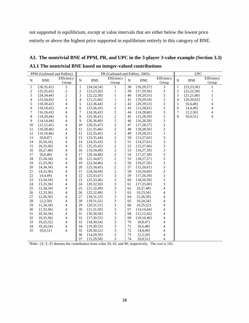
38

not supported in equilibrium, except at value intervals that are either below the lowest price

entirely or above the highest price supported in equilibrium entirely in this category of BNE.

A3. The nontrivial BNE of PPM, PR, and UPC in the 3-player 3-value example (Section 3.3)

A3.1 The nontrivial BNE based on integer-valued contributions PPM (Gailmard and Palfrey) PR (Gailmard and Palfrey, 2005) UPC

N BNE Efficiency Group N BNE Efficiency

Group N BNE Efficiency Group N BNE Efficiency

Group 1 {26,35,41} 2 1 {24,24,54} 1 38 {16,29,57} 3 1 {23,23,56} 1 2 {25,35,42} 2 2 {23,23,56} 1 39 {17,29,56} 3 2 {22,22,58} 1 3 {24,34,44} 2 3 {22,22,58} 1 40 {18,29,55} 3 3 {21,21,60} 1 4 {23,34,45} 2 4 {21,21,60} 1 41 {19,29,54} 3 4 {20,20,62} 1 5 {18,30,42} 4 5 {22,36,44} 2 42 {20,29,53} 3 5 {6,6,48} 4 6 {18,18,42} 4 6 {23,36,43} 2 43 {13,28,61} 3 6 {4,4,49} 4 7 {16,16,43} 4 7 {24,36,42} 2 44 {14,28,60} 3 7 {2,2,50} 4 8 {14,29,44} 4 8 {25,36,41} 2 45 {15,28,59} 3 8 {0,0,51} 4 9 {14,14,44} 4 9 {26,36,40} 2 46 {16,28,58} 3

10 {12,12,45} 4 10 {20,35,47} 2 47 {17,28,57} 3 11 {10,28,46} 4 11 {21,35,46} 2 48 {18,28,56} 3 12 {10,10,46} 4 12 {22,35,45} 2 49 {19,28,55} 3 13 {8,8,47} 4 13 {23,35,44} 2 50 {13,27,62} 3 14 {6,34,34} 4 14 {24,35,43} 2 51 {14,27,61} 3 15 {6,33,36} 4 15 {25,35,42} 2 52 {15,27,60} 3 16 {6,27,48} 4 16 {19,34,49} 2 53 {16,27,59} 3 17 {6,6,48} 4 17 {20,34,48} 2 54 {17,27,58} 3 18 {5,34,34} 4 18 {21,34,47} 2 55 {18,27,57} 3 19 {5,33,36} 4 19 {22,34,46} 2 56 {19,27,56} 3 20 {4,34,34} 4 20 {23,34,45} 2 57 {15,26,61} 3 21 {4,33,36} 4 21 {24,34,44} 2 58 {16,26,60} 3 22 {4,4,49} 4 22 {22,33,47} 3 59 {17,26,59} 3 23 {3,34,34} 4 23 {23,33,46} 3 60 {18,26,58} 3 24 {3,33,36} 4 24 {20,32,50} 3 61 {17,25,60} 3 25 {2,34,34} 4 25 {21,32,49} 3 62 {6,27,48} 4 26 {2,33,36} 4 26 {22,32,48} 3 63 {0,23,56} 4 27 {2,26,50} 4 27 {18,31,53} 3 64 {2,26,50} 4 28 {2,2,50} 4 28 {19,31,52} 3 65 {0,24,54} 4 29 {1,34,34} 4 29 {20,31,51} 3 66 {0,25,52} 4 30 {1,33,36} 4 30 {21,31,50} 3 67 {14,14,44} 4 31 {0,34,34} 4 31 {16,30,56} 3 68 {12,12,45} 4 32 {0,33,36} 4 32 {17,30,55} 3 69 {10,10,46} 4 33 {0,25,52} 4 33 {18,30,54} 3 70 {8,8,47} 4 34 {0,24,54} 4 34 {19,30,53} 3 71 {6,6,48} 4 35 {0,0,51} 4 35 {20,30,52} 3 72 {4,4,49} 4

36 {14,29,59} 3 73 {2,2,50} 4

37 {15,29,58} 3 74 {0,0,51} 4 Note: {X, Y, Z} denotes the contribution from value 29, 45, and 90, respectively. The cost is 102.

39

A3.2 The nontrivial BNE in the most efficient group with a contribution precision of 0.1 N UPC PR 1 {19.1, 19.1, 63.8} {20.3, 20.3, 61.4} 2 {19.2, 19.2, 63.6} {20.4, 20.4, 61.2} 3 {19.3, 19.3, 63.4} {20.5, 20.5, 61} 4 {19.4, 19.4, 63.2} {20.6, 20.6, 60.8} 5 {19.5, 19.5, 63} {20.7, 20.7, 60.6} 6 {19.6, 19.6, 62.8} {20.8, 20.8, 60.4} 7 {19.7, 19.7, 62.6} {20.9, 20.9, 60.2} 8 {19.8, 19.8, 62.4} {21, 21, 60} 9 {19.9, 19.9, 62.2} {21.1, 21.1, 59.8} 10 {20, 20, 62} {21.2, 21.2, 59.6} 11 {20.1, 20.1, 61.8} {21.3, 21.3, 59.4} 12 {20.2, 20.2, 61.6} {21.4, 21.4, 59.2} 13 {20.3, 20.3, 61.4} {21.5, 21.5, 59} 14 {20.4, 20.4, 61.2} {21.6, 21.6, 58.8} 15 {20.5, 20.5, 61} {21.7, 21.7, 58.6} 16 {20.6, 20.6, 60.8} {21.8, 21.8, 58.4} 17 {20.7, 20.7, 60.6} {21.9, 21.9, 58.2} 18 {20.8, 20.8, 60.4} {22, 22, 58} 19 {20.9, 20.9, 60.2} {22.1, 22.1, 57.8} 20 {21, 21, 60} {22.2, 22.2, 57.6} 21 {21.1, 21.1, 59.8} {22.3, 22.3, 57.4} 22 {21.2, 21.2, 59.6} {22.4, 22.4, 57.2} 23 {21.3, 21.3, 59.4} {22.5, 22.5, 57} 24 {21.4, 21.4, 59.2} {22.6, 22.6, 56.8} 25 {21.5, 21.5, 59} {22.7, 22.7, 56.6} 26 {21.6, 21.6, 58.8} {22.8, 22.8, 56.4} 27 {21.7, 21.7, 58.6} {22.9, 22.9, 56.2} 28 {21.8, 21.8, 58.4} {23, 23, 56} 29 {21.9, 21.9, 58.2} {23.1, 23.1, 55.8} 30 {22, 22, 58} {23.2, 23.2, 55.6} 31 {22.1, 22.1, 57.8} {23.3, 23.3, 55.4} 32 {22.2, 22.2, 57.6} {23.4, 23.4, 55.2} 33 {22.3, 22.3, 57.4} {23.5, 23.5, 55} 34 {22.4, 22.4, 57.2} {23.6, 23.6, 54.8} 35 {22.5, 22.5, 57} {23.7, 23.7, 54.6} 36 {22.6, 22.6, 56.8} {23.8, 23.8, 54.4} 37 {22.7, 22.7, 56.6} {23.9, 23.9, 54.2} 38 {22.8, 22.8, 56.4} {24, 24, 54} 39 {22.9, 22.9, 56.2} {24.1, 24.1, 53.8} 40 {23, 23, 56} {24.2, 24.2, 53.6} 41 {23.1, 23.1, 55.8} 42 {23.2, 23.2, 55.6} Note: {X, Y, Z} denotes the contribution from value 29, 45, and 90, respectively. The cost is 102.

With a contribution precision of 0.1, PPM has 584 nontrivial equilibria, none of which are in the

most efficient group; PR has 5330, 40 of which in the most efficient group; UPC has only 73 , 42

of which in the most efficient group. Also, notice that the eight most efficient BNE in UPC and

PR (four for each) based on the integer-valued contributions are still included (in bold).

40

References

Alboth, D., Lerner, A. and Shalev, J. (2001), Profit maximizing in auctions of public goods,

Journalof Public Economic Theory, 3 (4): 501-525.

Bagnoli, M. and Lipman, B. L. (1989), Provision of Public-Goods - Fully Implementing the Core

through Private Contributions, Review of Economic Studies, 56 (4): 583-601.

Bagnoli, M. and McKee, M. (1991), Voluntary Contribution Games - Efficient Private Provision

of Public-Goods, Economic Inquiry, 29 (2): 351-366.

Barbieri, S. and Malueg, D. A. (2008), Private Provision of a Discrete Public Good: Efficient

Equilibria in the Private-information Contribution Game, Economic Theory, 37 (1): 51-80.

Barbieri, S. and Malueg, D. A. (2010a), Threshold uncertainty in the private-information

subscription game, Journal of Public Economics, 94 (11-12): 848-861.

Barbieri, S. and Malueg, D. A. (2010b), Profit-Maximizing Sale of a Discrete Public Good via

the Subscription Game in Private-Information Environments, B E Journal of Theoretical

Economics, 10 (1): Article 5.

Borgers, T., Krahmer, D., and Strausz, R (2015), An Introduction to the Theory of Mechanism

Design, Oxford University Press, in press.

Bush, G., Hanley, N., Moro, M., and Rondeau, D. (2013), Measuring the Local Costs of

Conservation: A Provision Point Mechanism for Eliciting Willingness to Accept

Compensation, Land Economics, 89 (3):490-513.

Champ, P. A., Flores, N. E., Brown, T. C. and Chivers, J. (2002), Contingent valuation and

incentives, Land Economics, 78 (4): 591-604.

Chen, Y. (2008). Incentive-compatible Mechanisms for Pure Public Goods: A Survey of

Experimental Research. In: and Charles, R.P. and. Smith, V.L., Editors, 2008. Handbook of

Experimental Economics Results. North-Holland, Amsterdam, The Netherlands, Volume 1:

625-643.

Davis, D. and Holt, C. (1993), Experimental Economics, Princeton University Press, Princeton,

NJ, p.317 – 379.

Fischbacher, U. (2007), z-Tree: Zurich Toolbox for Ready-made Economic Experiments,

Experimental Economics, 10 (2): 171-178.

Gailmard, S. and Palfrey, T. R. (2005), An experimental comparison of collective choice

procedures for excludable public goods, Journal of Public Economics, 89 (8): 1361-1398.

41

Haskell, J., Uchida, E., Swallow, S.K., and Uchida, H. (2010), Willingness-to-pay for ecosystem

services in Rhode Island: Do payment elicitation mechanisms matter? University of Rhode

Island working paper, Retrieved

from http://www.webmeets.com/WCERE/2010/prog/viewpaper.asp?pid=1037

Isaac, R. M., Schmidtz, D. and Walker, J. M. (1989), The assurance problem in a laboratory

market, Public Choice, 62 (3): 217-236.

Li, Z., Anderson, C. M., and Swallow, S. K., (2014), Uniform price mechanisms for threshold

public goods provision with complete information: an experimental investigation, working

paper.

Laussel, D. and Palfrey, T. R. (2003), Efficient Equilibria in the Voluntary Contributions

Mechanism with Private Information, Journal of Public Economic Theory, 5 (3): 449-478.

Ledyard, J.O., (1995). Public goods: a survey of experimental research. In: Kagel, J.H. and Roth,

A.E., Editors, 1995. The Handbook of Experimental Economics, Princeton University Press,

Princeton, New Jersey, pp. 111–194.

Marks, M. and Croson, R. (1998), Alternative rebate rules in the provision of a threshold public

good: An experimental investigation, Journal of Public Economics, 67 (2): 195-220.

McBride, M. (2006), Discrete public goods under threshold uncertainty, Journal of Public

Economics, 90 (6-7): 1181-1199.

Menezes, F. M., Monteiro, P. K. and Temimi, A. (2001), Private provision of discrete public

goods with incomplete information, Journal of Mathematical Economics, 35 (4): 493-514.

Moulin, H. (1994), Serial Cost-Sharing of Excludable Public-Goods, Review of Economic

Studies, 61 (2): 305-325.

Nitzan, S. and Romano, R. E. (1990), Private Provision of a Discrete Public Good with

Uncertain Cost, Journal of Public Economics, 42 (3): 357-370.

Rondeau, D., Poe, G. L. and Schulze, W. D. (2005), VCM or PPM? A comparison of the

performance of two voluntary public goods mechanisms, Journal of Public Economics, 89

(8): 1581-1592.

Rondeau, D., Schulze, W. D. and Poe, G. L. (1999), Voluntary revelation of the demand for

public goods using a provision point mechanism, Journal of Public Economics, 72 (3): 455-

470.

Schwartz, J. A. and Wen, Q., (2013), A characterization for dominant strategy implementation,

42

Frontiers of Economics in China, 8 (1): 1-18.

Spencer, M. A., Swallow, S. K., Shogren, J. F. and List, J. A. (2009), Rebate rules in threshold

public good provision, Journal of Public Economics, 93 (5-6): 798-806.

Swallow, S.K., Smith, E.C., Uchida, E. and Anderson, C.M. (2008), Ecosystem Services beyond

Valuation, Regulation, and Philanthropy: Integrating Consumer Values into the Economy,

Choices, 23 (2): 47-52.

Swallow, S. K. (2013), Demand-side Value for Ecosystem Services and Implications for

Innovative Markets: Experimental Perspectives on the Possibility of Private Markets for

Public Goods, Agricultural and Resource Economics Review, 42 (1): 33-56.